1

U.S. Shrimp Market Integration

Frank Asche,1 Lori S. Bennear,2,3,4 Atle Oglend,1 and Martin D. Smith2, 4,*

1. Department of Industrial Economics, University of Stavanger, 4036 Stavanger, Norway

2. Nicholas School of the Environment, Duke University, Box 90328, Durham, NC 27701

3. Sanford School of Public Policy, Duke University

4. Department of Economics, Duke University

* Corresponding author.

Email: marsmith@duke.edu, ph: (919) 613-8028, fax: (919) 684-8071

Abstract: Recent supply shocks in the Gulf of Mexico—including hurricanes, the Deepwater

Horizon oil spill, and the seasonal appearance of a large dead zone of low oxygen water

(hypoxia)—have raised concerns about the economic viability of the U.S. shrimp fishery.

The ability for U.S. shrimpers to mediate supply shocks through increased prices hinges on

the degree of market integration, both among shrimp of different sizes classes and between

U.S. wild caught shrimp and imported farmed shrimp. We use detailed data on shrimp prices

by size class and import prices to conduct a co-integration analysis of market integration in

the shrimp industry. We find significant evidence of market integration, suggesting that the

law of one price holds for this industry. Hence, in the face of a supply shocks, prices do not

rise and instead imports of foreign farmed fish increase.

JEL: Q22

Keywords: seafood trade, market integration, environmental shocks

Acknowledgments: Financial support for this research was provided by the National Oceanic

and Atmospheric Administration Grant# 2162501 and by the Research Council of Norway.

The authors thank Jim Nance for providing the U.S. shrimp data and for helpful discussions.

2

U.S. Shrimp Market Integration

Abstract: Recent supply shocks in the Gulf of Mexico—including hurricanes, the Deepwater

Horizon oil spill, and the seasonal appearance of a large dead zone of low oxygen water

(hypoxia)—have raised concerns about the economic viability of the U.S. shrimp fishery.

The ability for U.S. shrimpers to mediate supply shocks through increased prices hinges on

the degree of market integration, both among shrimp of different sizes classes and between

U.S. wild caught shrimp and imported farmed shrimp. We use detailed data on shrimp prices

by size class and import prices to conduct a co-integration analysis of market integration in

the shrimp industry. We find significant evidence of market integration, suggesting that the

law of one price holds for this industry. Hence, in the face of a supply shocks, prices do not

rise and instead imports of foreign farmed fish increase.

JEL: Q22

Keywords: seafood trade, market integration, environmental shocks

1. Introduction

Shrimp is the world’s most valuable seafood product, accounting for 17% of the global

seafood trade in 2006 (FAO 2009). Although more than half of the world’s shrimp are farmed

now, significant wild shrimp fisheries remain in many parts of the world, including in the

Gulf of Mexico and along the East Coast of the United States. Figure 1 depicts global shrimp

production broken down by farmed and wild shrimp. Production of wild shrimp increased in

recent decades but leveled off in 2003 at just over 3 million metric tons. Farmed shrimp

production increased at even faster rates and reached a production of 3.5 million metric tons

in 2009 for a combined global supply of over 6.6 million metric tons. This increased

production has fueled an increased trade in shrimp. As for most farmed species, the markets in

the EU, Japan and the U.S. have been the most targeted, since these are the markets with the

highest willingness to pay.

Consumption of shrimp in the United States reflects the global surge in shrimp production.

Shrimp ranked first in 2004 U.S. per capita seafood consumption at 4.2 pounds, nearly a

3

pound more than the second ranked seafood category (canned tuna with 3.3 pounds per

capita) (NRC 2007). In 2010, shrimp consumption remained high at 4.0 pounds per capita

compared to 2.7 pounds per capita of canned tuna, and consumption of all fillets and steaks

aggregated across species amounted to only 5.0 pounds per capita (National Marine Fisheries

Service 2011). Much of this consumption comes from imported farm-raised shrimp, as the

U.S. has developed into the world’s largest shrimp import market (Anderson, 2003). In 1980,

domestic shrimp had a 43% market share, but that share declined to 12% by 2001 (Mukherjee

and Segerson 2011). In spite of the declining market share, the U.S. still maintains a large

wild shrimp fishery with 80% caught in the Gulf of Mexico (Mukherjee and Segerson 2011).

The U.S. domestic shrimp fishery has three main species: brown, pink and white shrimp, the

largest being brown. Brown shrimp landings in the Gulf over the past decade ranged from

33,000 to 71,000 metric tons with landed value between $137 million and $355 million. For

pink, landings ranged from 2,300 to 6,900 metric tons with landed value between $10 million

and $39 million. For white, landings ranged from 37,000 to 67,000 metric tons with landed

value between $141 million and $252 million .1

Understanding how integrated the markets for domestic wild-caught shrimp fisheries are with

markets for farmed shrimp imports is important for several reasons. First, the rapid increase

in farmed shrimp production coupled with large domestic wild-caught fisheries has created

trade disputes in the EU and in the U.S. The U.S., for example, enacted trade restrictions on

shrimp from a group of six named countries (all in Asia or Latin America) in 2004 after

domestic fishermen filed anti-dumping complaints against several shrimp exporting countries

(Keithly and Poudel, 2008). Second, diseases have been an issue for farmed shrimp. The

reduced growth rates in farmed shrimp production in the 1990s can largely be attributed to the

white spot disease (Anderson, 2003). Third, there are significant environmental shocks that

1 http://www.st.nmfs.noaa.gov/st1/commercial/landings/annual_landings.html

4

affect the supply of domestic wild-caught shrimp. For U.S. shrimp fishermen, hypoxia—most

notably the seasonal dead zone in the Gulf of Mexico—has been a reoccurring phenomenon

that potentially influences aggregation, production, and the size distribution of shrimp (Craig

2011; Huang, Smith, and Craig, 2010; Huang et al. 2011). Hurricanes Katrina and Rita caused

significant shrimp supply disruptions through destruction of shrimp vessels and processing

facilities (Buck 2005), while rising fuel prices are particularly costly for wild-caught shrimp

because trawling is fuel-intensive (Ran, Keithly, Kazmierczak 2011), Moreover, costs of

complying with the U.S. requirement for shrimp trawlers to use Turtle Excluder Devices

decreased domestic supply (Mukherjee and Segerson 2011). The degree of market integration

affects how these environmental and economic stressors affect prices. The impact of all of

these stressors (trade, production costs, disease, and environmental) will have a strong impact

on the price determination process if the markets are not integrated, while the impact will be

weaker in a larger and more integrated shrimp market. The rationale is that consumers can

substitute other species (or substitute across wild or farmed) if the supply of one species

becomes scarce due to a production shock.

Despite being the world’s most important aquaculture species and comparably significant

global capture landings, there are relatively few studies shedding light on the price

determination process for shrimp. Vinuya (2007) is an exception, indicating that there is a

global market for farmed shrimp. We investigate the extent of the shrimp market by testing

for market integration using prices. Time series analysis of market integration has been used

for a number of seafood products in recent decades. It is particularly useful when there is a

large number of products/markets of interest, as demand analysis in such cases is not feasible

(Asche, Gordon and Hannesson, 2004). Time series analysis can also be a flexible approach

by allowing tests across geographically distinct markets, different species, and different

product forms. If prices are stationary, ordinary regression analysis can be used (Squires,

5

Herrick Jr., and Hastie, 1989; Asche, Gordon and Hannesson, 2004). But if prices are

nonstationary, cointegration analysis is the appropriate econometric tool.2

The paper is proceeds as follows. The data are described in Section 2. Section 3 contains a

description of the time-series methods used for the empirical tests of market integration.

Section 4 reports the results. Section 5 concludes with discussion and implications for the

shrimp market.

2. Data

Our data set consists of monthly prices covering the period of June 1990 through December

2008. The prices of brown, pink and white shrimp by size are for the Gulf of Mexico shrimp

fishery and are computed by aggregating daily landings values and quantities that are

recorded in the NOAA’s SHRCOM database. SHRCOM is the primary source of micro-data

used for fisheries management in the Gulf of Mexico. The import prices are U.S. import

prices from the U.S. Department of Commerce www.st.nmfs.noaa.gov/st1/trade).

Shrimp size is measured as the number of shrimp per pound. Hence, a higher number implies

a smaller average size for the shrimp. In the raw data, prices are available for the three species

in eight size categories for a total of 24 price time series. Figures 2 shows the prices by size

class for brown shrimp. Price series for pink and white shrimp appear similar (Asche et al.

2011). In all cases, larger sizes are more valuable per pound, and there is substantial variation

in the price level by size. However, the price development of the different sizes appears to

follow a common trend. Within each species, price increases (decreases) for one size tend to

2 Since most seafood prices are found to be nonstationary, cointegration is the most commonly used empirical

tool to test for market integration (Gordon, Salvanes and Atkins, 1993; Bose and McIlgrom, 1996; Gordon and

Hannesson, 1996; Asche, Bremnes and Wessells, 1999; Asche, 2001; Jaffry et al, 2001; Asche et al, 2005;

Nielsen, 2005; Nielsen et al 2007; Norman-López and Asche, 2008; Nielsen, Smit and Guillen, 2009; Norman-

López, 2009).

6

translate into price increases (decreases) for each of the other sizes. Visually, Figure 2

suggests market integration, which we formally test in Section 4.

To compare the price development of U.S. shrimp with imports, the different weight classes

are aggregated to avoid the curse of dimensionality.3 This weighting is done by constructing

a Fisher Price index for each of the three species. For imported shrimp, the category “shell-on

frozen” is used. This category is the closest to the largest volumes for domestically produced

shrimp because it is relatively unprocessed. In contrast, products like breaded shrimp or

shrimp in frozen meals contain significant value added that could distort inferences about

market integration.

Before conducting formal tests of market integration, the time series properties of the prices

must be investigated. The results from Augmented Dickey-Fuller (ADF) tests are reported in

Table 1. Nearly all of the individual size-based price series are nonstationary in levels but

stationary in first differences. The exceptions are small brown shrimp and very large pink

shrimp that appear stationary in levels. All indexed prices are nonstationary in levels but

stationary in first differences. The price series are, accordingly, integrated of order one, and

cointegration analysis is the appropriate tool. This finding is as expected and in line with what

is found for most seafood prices.

3. Methods4

Let p1t be the price in one market and p2t the price in another. The basic relationship of

interest for investigating market integration using time-series price data is the following:

tt pp 21 lnln , (1)

3 Hendry (1995) provides a good discussion of the curse of dimensionality in time series analysis. 4 This section largely follow Asche, Gordon and Hannesson (2004).

7

where is a constant term that captures differences in the levels of the prices and

indicates the relationship between the prices. If = 0, there is no relationship between the

prices, whereas if = l the prices are proportional. When prices are proportional, the relative

price is stationary, a phenomenon known as the Law of One Price (LOP). If differs from

zero but is not equal to one, there is a relationship between the prices, but the relative price is

not constant. Equation (1) describes the situation when prices adjust immediately. However,

there is often a dynamic adjustment pattern, which can be captured with lags of the two prices

(Ravallion, 1986; Slade, 1986). Even when dynamics are introduced, the long-run relationship

will have the same form as equation (1).

Since the late 1980s economists have known that traditional econometric tools cannot be used

when price series are non-stationary; standard statistical theory for inference breaks down in

these situations (Engle and Granger, 1987). Cointegration analysis is then the appropriate tool

to infer causal long-run relationships between non-stationary time series. There are two

common approaches to test for cointegration: the single equation-based Engle and Granger

test and the Johansen test (Johansen, 1988). Given that the price series are nonstationary and

integrated of the same order, the Engle and Granger test is performed by estimating equation

(1) and testing whether the residuals are stationary. Stationary residuals indicate that the two

price series are cointegrated.

The Johansen test is appropriate for a system of prices, and accordingly allows for more than

one long-run relationships. Moreover, it allows for hypothesis testing on the parameters in the

cointegration vector and exogeneity tests. The Johansen method is based on a vector

autoregressive error correction model (VECM). With a vector, Pt, containing the n prices., to

test for cointegration the system can be written as

8

1

1

k

t i t i k t k t

i

P P P e

(2)

The matrix contains the parameters in the long-run relationships (the cointegration vectors).

Given r cointegrating vectors, one can factorize k , where both and are (n r)

matrices. The -matrix contains the cointegrating vectors and the adjustment parameters.

We use the trace test to determine the rank of . Tests with respect to the structural

relationship between the prices (markets) are tests of restrictions on the parameters in the

cointegrating vectors, . Information about the existence of a central market is formally

conducted through exogeneity tests on the coefficients and through examination of the

integrating factors.

To illustrate, consider the case with only two price series, A and B. Assume that the two price

series are nonstationary but cointegrated and that one lag is sufficient to capture the dynamics.

The price relationships (suppressing the error terms) can be represented as

1 1

1 2

2 1

A A

t t

B B

t t

ap pb b

ap p

(3)

If b1 = -b2, the prices are proportional and the LOP holds. Usually, b1 is normalized, so that

the null hypothesis is b2 = -1. The parameters ia measure the impact of deviations from the

long-run relationship and is normally denoted as the adjustment speed or factor loadings. In a

system with n price series and r stochastic trends, there can be at most r exogenous variables

(Johansen and Juselius 1994). With the structure expected in efficiently functioning

commodity markets, n-1 cointegrating vectors and one stochastic trend are expected (Asche,

Bremnes and Wessells, 1999; Gonzalez-Rivera and Helfand, 2001).

4. Empirical Results

9

The sheer number of prices in the different shrimp size categories and species makes it

virtually impossible to investigate the degree of market integration in one large system due to

the curse of dimensionality. Moreover, Asche and Guttormsen (2001) note that prices for

different weight classes are likely to be proportional, and if that is the case, they can be

aggregated using the Generalized Composite Commodity Theorem of Lewbel (1996). We

thus commence our analysis by testing for market integration for each of the three species

where prices by size are available. We then investigate the relationships among the three

species and imports.

For the separate species, the most interesting issue is whether the market is fully integrated or

whether there exist different price determination processes by size. Supply shocks could affect

different size classes differently due to spatio-temporal dynamics of the fishery and individual

species life histories. Separate markets for each size would suggest that shocks that affect one

size class would not propagate through to other size classes. This outcome, in turn, would

affect the level of price compensation in the affected market. We thus use Engle and Granger

tests for the size classes within each species and start out by imposing proportionality, i.e.

= l in equation (1). If this hypothesis is rejected, we continue to test for cointegration without

this restriction to distinguish the case of imperfect market integration from no market

integration.

The results of the Engle and Granger test are reported in Table 2. For nearly all price pairs,

the null hypothesis of nonstationarity is rejected. The only exceptions are for the smallest size

classes that constitute small shares of the total landings. Hence, we conclude that for all the

three species, there is strong evidence of a common price determination process and that the

prices move proportionally over time. This conclusion implies that one can construct an

aggregate price for each species.

10

To investigate the relationships among the prices of the three species and the import price, a

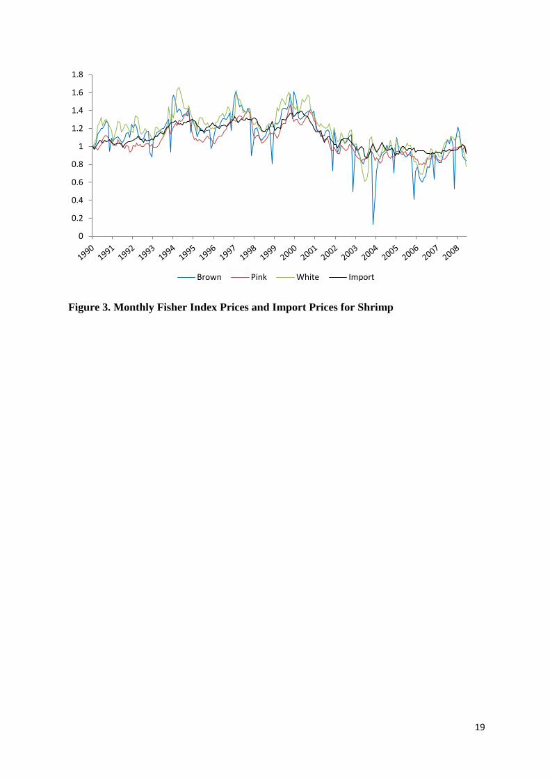
Johansen test is used. Here we used the indexed prices depicted in Figure 3. The number of

lags is chosen using the AIC and is found to be 14. A set of dummies is included to account

for seasonality. The likelihood ratio test of Johansen and Juselius (1991) indicates that the

constant term should be included in the cointegrating vectors.

The cointegration tests are reported in Table 3. The results indicate that the system with four

prices contains three cointegrating vectors and accordingly one common stochastic trend. This

result is very robust with respect to model specification.

Normalized into bivariate relationships, the matrix containing the cointegrating vectors is

given as

𝛽 =

[

1 0 00 1 00 0 1

−1.113 −0.990 −1.124−0.000 −0.000 −0.001]

The b parameters are all relatively close to one, indicating that the prices are close to

proportional and the Law of One Price approximately holds. A test for this hypothesis is

distributed as χ2(3), and gives a test statistic of 4.595. With a p-value of 0.204, this hypothesis

accordingly is not rejected.

Trade restrictions on some named countries that are introduced to protect domestic producers

must influence the relationship between the domestic prices and the import price if they are to

have any effect. This can be tested by testing for structural breaks in the price relationships

(Asche, 2001). We do not find any evidence of any structural breaks in the relationships as a

test for a break at January 2000 gives a p-value of 0.720 and a test of a structural break in

January 2005 gives a p-value of 0.803. This supports the conclusion of Keithly and Poudel

11

(2008) who concluded that the trade restrictions primarily led to a reallocation of trade

patterns, with little benefit to domestic producers.

5. Discussion

Using detailed monthly price data for shrimp of various sizes we find significant evidence of

integration in the U.S. shrimp market. We test for proportionality in relative prices using all

possible price-pairs for different size classes, suggesting a common price determination

process and that the prices move proportionally over time.

We then construct an aggregate price index for each of three species of domestic wild-caught

shrimp and test for market integration between wild-caught shrimp and imports of farmed

shrimp. We again find significant evidence of market integration.

The degree of market integration, both among size classes and across farmed and wild-caught

shrimp has important implications for policy. First, in order for trade restrictions on imported

shrimp from named countries to protect domestic producers, these restrictions must influence

the relationship between the domestic prices and the import price. Market integration

suggests that this does not occur and trade restrictions act a as a shift in the type of imports,

for example by shifting to imports from non-named countries or of non-restricted shrimp (i.e.,

processed shrimp), rather than helping domestic producers.

Second, if farmed shrimp are subject to supply shocks from disease, market integration

implies that the domestic wild-caught fishery can replace supply from imports. The domestic

industry would benefit through expanded production but not through higher prices. Given the

wide range of domestic production and the influence of cost factors on supply, there is likely

room for such expansion. However, a caveat is in order. A major global shock to farmed

shrimp production that exceeds the magnitude of changes we observe in sample could lead to

the break down of market integration.

12

Finally, market integration has significant implications for how domestic wild-shrimp

fisherman can respond to certain environmental supply shocks. In North Carolina (a much

smaller market than Gulf of Mexico), there is evidence that hypoxia has decreased shrimp

production in the range of 13% but has not increased prices (Huang, Smith, and Craig 2010;

Huang et al. 2011). In the much larger Gulf of Mexico, there is emerging evidence that

hypoxia decreases the supply of large shrimp and increases the supply of smaller shrimp,

likely as a result of aggregation on the edge of hypoxic areas (Bennear, Kociolek, and Smith

2011; Craig 2011). Market integration suggests that the decreased supply of large shrimp

cannot be offset by an increase in price. Rather, imports of larger farmed shrimp will increase

to satisfy demand. Similarly, domestic supply shocks from hurricanes, oil spills, or fuel price

spikes cannot be offset by price increases. In particular, market integration suggests that the

economic losses from a significant decrease in 2010 domestic shrimp production – assuming

this decrease was caused by the Deepwater Horizon oil spill – was not likely offset by a price

increase. Market integration thus has important implications for the long-run economic

viability of the U.S. shrimp fishery. The losses from supply shocks are more consequential

for producers, and the various shocks are additive as economic challenges to the fishery. But

U.S. shrimp consumers are essentially unharmed. Market integration also implies that

regional demand shocks (positive or negative) are felt by the entire industry, but their effects

are dampened relative to how they would be felt in particular regions if markets were not

integrated.

One important caveat to our findings is that we have examined market integration in a period

(1990-2008) when shrimp imports have grown dramatically. While we find significant market

integration during this period, this integration could be recent and might not be found if

looking at subsets of the time domain. That is, it may be that earlier portions of the time

domain did not have market integration, and the implications for supply shocks during these

13

times varied. Hypoxia has been documented in the Gulf for two decades, though detailed data

are only available since the late 1990s. It may be that hypoxia had some ability to influence

prices in the past but no longer can due to the massive increase in imported shrimp.

A second caveat is to consider how the domestic wild-caught shrimp industry will react to the

many economic stressors it faces. Currently, there is growing interest amongst American

consumers in buying local food and wild-caught seafood in particular. The domestic shrimp

industry is attempting to capitalize on this interest .5 It remains to be seen whether domestic

wild-caught shrimp producers will successfully segment the market and undo the market

integration with imported farmed shrimp.

5 http://www.wildamericanshrimp.com/main.html

14

References

Anderson, J.L. 2003. The International Seafood Trade. Cambridge: Woodhead Publishing.

Asche, F. 2001. Testing the effect of an anti-dumping duty: The US salmon market. Empirical

Economics 26(2):343-55.

Asche, F., H. Bremnes and C.R. Wessells. 1999. Product Aggregation, Market Integration and

Relationships Between Prices: An Application to World Salmon Markets. American Journal

of Agricultural Economics 81(August):568-81.

Asche, F., D.V. Gordon and R. Hannesson. 2004. Tests for Market Integration and the Law of

One Price: The Market for Whitefish in France. Marine Resource Economics 19(2):195-210.

Asche, F. and A.G. Guttormsen. 2001. Patterns in the Relative Price for Different Sizes of

Farmed Fish. Marine Resource Economics 16(3):235-47.

Asche, F., et al. 2005. Competition between farmed and wild salmon: The Japanese salmon

market. Agricultural Economics 33:333-40.

Asche, F., L.S. Bennear, A. Oglend, and M.D. Smith. 2011. U.S. Shrimp Market Integration.

The Duke Environmental Economics Working Paper Series. Working Paper EE 11-09.

Durham, NC.

Bennear, L.S., E. Kociolek and M.D. Smith. 2011. Estimating the effect of hypoxia on the

Gulf Coast shrimp fishery. Selected Paper, AERE Summer Conference Seattle, WA, .

Bose, S. and A. McIlgrom. 1996. Substitutability Among Species in the Japanese Tuna

Market: A Cointegration Analysis. Marine Resource Economics 11(Fall):143-56.

Buck, E.H. (2005). Hurricanes Katrina and Rita: Fishing and Aquaculture Industries –

Damage and Recovery. CRS Report for Congress, RS22241. Washington DC, Congressional

Research Service.

Craig, J.K. 2011. Aggregation on the edge: Effects of hypoxia avoidance on the spatial

distribution of brown shrimp and demersal fishes in the northern Gulf of Mexico.

Forthcoming in Marine Ecology Progress Series.

Engle, R.F. and C.W.J. Granger. 1987. Co-integration and Error Correction: Representation,

Estimation and Testing. Econometrica 55(March):251-76.

FAO. 2009. The state of world fisheries and aquaculture 2008. Rome: FAO.

Gonzales-Rivera, G. and S.M. Helfand. 2001. The Extent, Pattern, and Degree of Market

Integration: A Multivariate Approach for the Brazilian Rice Market. American Journal of

Agricultural Economics 83(3):576-92.

Gordon, D.V. and R. Hannesson. 1996. On Prices of Fresh and Frozen Cod. Marine Resource

Economics 11(Winter):223-38.

15

Gordon, D.V., K.G. Salvanes and F. Atkins. 1993. A Fish Is a Fish Is a Fish: Testing for

Market Linkage on the Paris Fish Market. Marine Resource Economics 8(Winter):331-43.

Hendry, D.F. 1995. Dynamic Econometrics. Oxford: Oxford University Press.

Huang, L., L.A.B. Nichols, J.K. Craig and M.D. Smith 2012. Measuring Welfare Losses from

Hypoxia: The Case of North Carolina Brown Shrimp. forthcoming. Marine Resource

Economics.

Huang, L., M.D. Smith and J.K. Craig. 2010. Quantifying the Economic Effects of Hypoxia

on a Fishery for Brown Shrimp Farfantepenaeus aztecus. Marine and Coastal Fisheries:

Dynamics, Management, and Ecosystem Science 2:232-48.

Jaffry, S., et al. 2000. Price interactions between salmon and wild caught fish species on the

Spanish market. Aquaculture Economics and Management 4:157-68.

Johansen, S. 1988. Statistical Analysis of Cointegration Vectors. Journal of Economic

Dynamics and Control 12:231-54.

---. 1991. Estimation and Hypothesis Testing of Cointegration Vectors in Gaussian

Autoregressive Models. Econometrica 59:1551-80.

Keithly Jr., W.R. and P. Poudel. 2008. The Southeast U.S.A. Shrimp Industry: Issues Related

to Trade and Antidumping Duties. Marine Resource Economics 23(4):439-63.

Lewbel, A. 1996. Aggregation without Separability: A Generalized Composite Commodity

Theorem. American Economic Review 86(June):524-61.

Mukherjee, Z. and K. Segerson. 2011. Turtle Excluder Device Regulation and Shrimp

Harvest: The Role of Behavioral and Market Responses. Marine Resource Economics

26(2):173-89.

National Marine Fisheries Service. 2011. Fisheries of the United States 2010. Silver Spring,

MD: U.S. Department of Commerce.

Nielsen, M. 2005. Price Formation and Market Integration on the European First-hand Market

for Whitefish. Marine Resource Economics 20(2):185-202.

Nielsen, M., et al. 2007. Market Integration of Farmed Trout in Germany. Marine Resource

Economics 22:195-213.

Nielsen, M., J. Smit and J. Guillen. 2009. Market Integration of Fish in Europe. Journal of

Agricultural Economics 60(2):367-85.

Norman-López, A. 2009. Competition between different Wild and Farmed Species: The US

Tilapia Market. Marine Resource Economics 24:237-52.

Norman-López, A. and F. Asche. 2008. Competition between imported Tilapia and US catfish

in the US market. Marine Resource Economics 23(2):199-214.

16

Ran, T., W.R. Keithly Jr. and R.F. Kazmierczak. 2011. Location Choice Behavior of Gulf of

Mexico Shrimpers under Dynamic Economic Conditions. Journal of Agricultural and Applied

Economics 43(1):29-44.

Ravallion, M. 1986. Testing Market Integration. American Journal of Agricultural Economics

68(1):102-9.

Slade, M.E. 1986. Exogeneity Test of Market Boundaries Applied to Petroleum Products.

Journal of Industrial Economics 34:291-304.

Squires, D., S.F. Herrick Jr. and J. Hastie. 1989. Integration of Japanese and United States

Sablefish Markets. Fishery Bulletin 87(2).

Vinuya, F.D. 2007. Testing for Market Integration and the Law of One Price in World Shrimp

Markets. Aquaculture Economics and Management 11(3):243-65.

17

Figure 1. Global shrimp production by production method

0

500

1000

1500

2000

2500

3000

3500

4000M

illio

n M

etr

ic T

on

s

Aquaculture

Capture

18

Figure 2. Monthly Prices of Gulf of Mexico Brown Shrimp in Different Size Classes

0

2

4

6

8

10

12U

SD/p

ou

nd

<15 15-20 20-25 25-30 30-40 40-50 50-67 >67

19

Figure 3. Monthly Fisher Index Prices and Import Prices for Shrimp

0

0.2

0.4

0.6

0.8

1

1.2

1.4

1.6

1.8

Brown Pink White Import

20

TABLE 1. Augmented Dickey Fuller Unit Root Tests Shrimp Series

Level 1st Difference

Series Weight Class Constant Trend Constant Trend

Brown <15 -1.583 -2.217 -4.245** -4.342**

15-20 -1.176 -2.398 -4.453** -4.632**

20-25 -1.636 -2.853 -6.546** -7.805**

25-30 -1.069 -2.768 -7.302** -7.382**

30-40 -1.821 -3.312 -11.14** -11.14**

40-50 -2.540 -3.523* -3.595** -3.588*

50-67 -2.466 -3.138 -13.51** -13.49**

>67 -2.802 -3.790* -3.740** -4.321**

Pink <15 -4.672** -4.753** -7.707** -7.689**

15-20 -2.053 -2.081 -11.62** -11.59**

20-25 -2.199 -2.591 -16.02** -16.00**

25-30 -1.720 -2.238 -15.86** -15.84**

30-40 -1.956 -2.359 -14.44** -14.42**

40-50 -2.478 -2.466 -4.847** -4.861**

50-67 -2.113 -2.680 -9.537** -9.519**

>67 -2.965* -3.577* -7.519** -7.611**

White <15 -1.217 -2.116 -6.897** -6.512**

15-20 -0.7487 -2.014 -3.756** -3.884*

20-25 -1.767 -3.107 -9.597** -9.696**

25-30 -1.207 -2.441 -4.067** -4.113**

30-40 -1.851 -3.217 -4.394** -4.472**

40-50 -1.803 -2.848 -4.019** -4.040**

50-67 -2.546 -3.384 -7.075** -10.63**

>67 -2.368 -3.350 -4.266** -4.279**

Brown Fisher - -2.091 -3.242 -4.579** -4.038**

Pink Fisher - -2.069 -2.678 -11.35** -11.33**

White Fisher - -1.311 -2.385 -4.360** -4.399**

Import Fisher - -1.350 -2.469 -4.867** -7.143**

Note: * rejection at 5%, ** rejection at 1%

21

TABLE 2. Cointegration tests on spreads of species by weightclass

Species Spread ADF Spread ADF Spread ADF Spread ADF

Brown 15 – 1520 -4.884** 1520 – 2530 -5.467** 2025 – 3040 -5.488** 2530 – 67 -4.294**

15 – 2025 -4.494** 1520 – 2025 -4.941** 2025 – 4050 -5.089** 3040 – 4050 -8.601**

15 – 2530 -3.915* 1520 – 3040 -5.906** 2025 – 5060 -5.015** 3040 – 5060 -7.010**

15 – 3040 -4.601** 1520 – 4050 -4.800** 2025 – 67 -4.199** 3040 – 67 -3.275

15 – 4050 -4.336** 1520 – 5067 -4.491** 2530 – 3040 -4.389** 4050 – 5060 -3.240

15 – 5067 -3.862* 1520 – 67 -4.580** 2530 – 4050 -4.439** 4050 – 67 -3.206

15 – 67 -3.996* 2025 – 2530 -5.265** 2530 – 5060 -4.321** 5060 – 67 -3.159

Pink 15 – 1520 -7.484** 1520 – 2530 -4.650** 2025 – 3040 -5.285** 2530 – 67 -6.431**

15 – 2025 -4.561** 1520 – 2025 -3.788* 2025 – 4050 -4.442** 3040 – 4050 -4.344**

15 – 2530 -7.773** 1520 – 3040 -6.025** 2025 – 5060 -3.600* 3040 – 5060 -4.368**

15 – 3040 -6.153** 1520 – 4050 -5.403** 2025 – 67 -5.970** 3040 – 67 -7.338**

15 – 4050 -6.507** 1520 – 5067 -4.445** 2530 – 3040 -5.102** 4050 – 5060 -5.193**

15 – 5067 -5.569** 1520 – 67 -5.221** 2530 – 4050 -4.670** 4050 – 67 -6.635**

15 – 67 -7.130** 2025 – 2530 -5.314** 2530 – 5060 -4.493** 5060 – 67 -9.303**

White 15 – 1520 -4.027** 1520 – 2530 -3.526* 2025 – 3040 -5.050** 2530 – 67 -5.267**

15 – 2025 -3.478* 1520 – 2025 -3.458* 2025 – 4050 -4.361** 3040 – 4050 -5.807**

15 – 2530 -3.770* 1520 – 3040 -4.159** 2025 – 5060 -4.210** 3040 – 5060 -6.085**

15 – 3040 -4.043** 1520 – 4050 -4.030** 2025 – 67 -3.676* 3040 – 67 -5.998**

15 – 4050 -3.712* 1520 – 5067 -4.265** 2530 – 3040 -5.178** 4050 – 5060 -6.692**

15 – 5067 -4.013** 1520 – 67 -3.778* 2530 – 4050 -4.159** 4050 – 67 -3.311

15 – 67 -3.386 2025 – 2530 -4.551** 2530 – 5060 -4.471** 5060 – 67 -3.129

Note: * rejection at 5%, ** rejection at 1%

22

TABLE 3. Cointegration Analysis for Brown,Pink,White and Imported Shrimp Prices Rank Eigenvalue Trace stat. 5% cv. Max eigenvalue stat. 5% cv.

0 - 117.464* 62.99 47.485* 31.46 1 0.20411 69.979* 42.44 36.786* 25.54 2 0.16210 33.192* 25.32 25.203* 18.96 3 0.11412 7.9883 12.25 7.988* 12.52 4 0.03768