1

Urbanisation, inequality and economic growth:

Evidence from Indian states and towns

Background note for the World Development Report 2009

Massimiliano Calì1

June 2008

I empirically address three important aspects of the urbanisation process in India:

rural-urban disparities and their relation with economic development; the relation

between urbanisation and growth; and the convergence hypothesis in cities’ growth.

The results support the idea of a U-shaped relation between rural-urban disparities in

socio-economic indicators and the level of economic development. Also although the

level of urbanisation and that of economic development go hand in hand across Indian

states over time, this relation is not strong. On the other hand, the rate of urbanisation

(i.e. how fast a state urbanises) and the rate of growth appear to be negatively

correlated. Finally, using a large dataset of Indian towns for the 20th century, I find

that there is a tendency towards convergence in growth rates among Indian towns

across all decades of the century. Other things being equal smaller towns grow faster

than large ones. This somewhat contrasts the fears of urban concentration with large

towns growing too quickly relative to the other towns.

1 Research Officer with the Overseas Development Institute, London (m.cali@odi.org.uk). I would like

to thank Hiro Uchida, Chroching Goh and Steve Gibbons for helpful suggestions. Funding from the

World Bank is gratefully acknowledged. The usual disclaimer applies.

2

1. Introduction and scope of the work

The structural transformation of an economy during the process of development is a

well established fact. In this process a rural population mainly employed in agriculture

turns into an urban one shifting towards industry and eventually services. Such a

process has some clear association with the rural-urban distribution of income within

countries as well as with their rate of growth. This paper is concerned with both of

these macro aspects of the urbanisation. It also aims to describe the nature of the

urbanisation process by testing for convergence as well as for persistence in growth

rates of cities. This provides a complementary view of the urban transformation of a

country to that of the macro-analysis.

1.1. Rural-urban inequality and economic development

The relationship between income distribution and economic development was first

identified by the seminal work of Kuznets (1955). His work hypothesised an inverted

U-shaped relationship between income and inequality: the initial stage of a country’s

economic development would be associated with rising inequalities up to a point

(during the middle-income stage of development), after which inequalities would

decrease with income per capita.

Following the decomposition of income inequality along a spatial dimension into a

within group and a between groups components, Kuznets’ hypothesis can be divided

into a within-sector and a between-sector and inequality (Frankema, 2006). The

former relates to rural-urban income inequality while the latter refers to intra-urban

and intra-rural inequalities. Rural-urban inequality usually explains the majority of a

country’s inequality in the early stages of the development process. Kanbur and

Zhang (1999) find for instance that over 70% of overall inequality in China was

explained by the rural-urban component over the period 1983-1995.2 Kuznets’

hypothesis holds that this component of inequality mimics the relationship between

overall inequality and income growth. In the initial phase of development the urban

sector expands due to rapid urban labour productivity growth. This widens the rural-

urban income gap as increase in rural productivity is more sluggish. After peaking,

2 This share was over 80% for inland areas.

3

rural-urban dualism declines and eventually dissolves in the long run as rural labour

productivity catches up following rural-urban migration and technology and demand

spill-overs from the urban sector.

This relation has important similarities with the one between regional inequality and

economic development within a country. The work in this area has been inspired by

the analysis of Williamson (1965), who found that regional disparities would bear a

typical inverted U shaped relation with income per capita. The theoretical intuition for

this pattern is related to the tension between centripetal forces towards concentration

of economic activity and centrifugal forces towards dispersion. The former, driven by

agglomeration economies, would prevail in the early stages of development, causing a

process of cumulative causation which reinforces the initial advantage of the more

advanced region/location. This concentration process would continue until the level of

economic activity reaches a threshold, after which the congestion costs from

agglomeration (centrifugal forces) would offset the centripetal forces, dispersing

economic activity again. The two models appear to be complementary with the latter

providing some micro-fundamentals for explaining the divergence-convergence

hypothesis of the former.

While the relationship between regional inequalities and development has been matter

of an increasing interest, little empirical evidence is available on the rural-urban

inequality-income relation.3 The lack of such evidence may help explain why the

overall Kuznets’ hypothesis has never reached an empirical consensus, although it

seems to fit a number of countries’ development processes, including the recent

growth experience of China. The failure to separate the sub-components of the

inequality-income relationship may lead to overlook countervailing forces hidden in

the catch-all income inequality variable. A vivid illustration of this point is provided

by Frankema (2006), who finds that the persistent personal income inequality of Latin

America in the 20th century is also associated to declining rural-urban inequality.

The first section of this paper focuses on a specific component of inequality, namely

rural-urban inequality. In particular, it analyses the relationship between rural-urban

3 Bourguignon and Morrison (1998) note for instance that recent development literature has by and

large ignored the analysis of rural-urban dualism.

4

inequality and economic development in Post-Independence India. The analysis uses

particular measures of rural-urban inequality, by and large based on poverty

indicators. Although such measures are obviously inter-related with more traditional

measure of inequality (calculated on absolute incomes), they add a further interesting

angle to the debate: that is essentially that policy should be more concerned with

poverty than with inequality per se. For instance, transfers among those above the

poverty line that “reduce inequality without touching poverty should be of second-

order concern” (Eastwood and Lipton, 2000, p. 21). Moreover, unlike most literature

concerned with rural-urban inequality, which has primarily looked at the evolution of

this inequality over time, this study tries to identify the relationship between income

per capita and rural-urban differences in poverty indices. Understanding the nature of

this relation would be important inter alia in order to assess whether the economic

development process has an urban, a rural or a neutral bias.

1.2. Urban growth and economic growth

A complementary question concerns the extent to which urbanisation is related to the

process of economic development. The literature has so far quite clearly established

that economic development is almost invariably associated with the expansion of the

urban sector (e.g. Henderson, 2004 and Davis and Henderson, 2003). But the evidence

is much thinner on the question of what type of relationship exists between economic

development and the speed of urbanization. Do the two processes map one to one so

that faster urbanization is systematically associated with faster economic growth?

Answers to this question are important from a policy standpoint as they are related to

how efficient the reallocation of resources from the rural to the urban sector is in the

short-run. This reallocation is inherent to the long-term process of development, but in

the short-run too slow (or too rapid) rural-urban migration may cause imbalances

reflected in slower economic growth. Au and Henderson (2006) find that migration

restrictions in China have been associated with smaller than optimal cities’ size,

which in turn has entailed average labour productivity losses of 30% relative to the

optimal size.4

4 The optimal size is defined as the size at which the net output per worker is maximised. This is only

an indicative figure derived from a statistical exercise, it is still suggestive of some potential substantial

productivity losses from undersized cities.

5

Another related implication of this analysis is that it can shed some light on the net

effects of increased productivity and increased congestion in the process of cities’

growth. These two effects drive the dynamics of urban productivity and net wages as

urban areas expand. Standard urban economics literature shows that agglomeration

economies increase productivity and wages but these effects are counterbalanced by

increased costs of congestion as the city grows (see Combes et al., 2005). As a large

part of the urbanisation process is accounted for by the growth of existing urban areas,

the speed of urbanisation indicates how quickly these areas are growing. If rapid

urbanisation is associated with faster economic growth, this may suggest that the

agglomeration benefits from larger cities’ size are likely to be larger than the

diseconomies from increased congestion. Section 3 will examine this question with

Indian states’ data.

1.3. Size and growth of cities

Finally, I consider the micro-counterpart of the macro analysis described above, by

inspecting the nature of the urbanisation process. The analysis tries to explore the

determinants of the growth (in size) of Indian cities, focusing in particular on the

question of convergence growth rates. This question links back to the copious

literature on convergence in economic growth in the tradition of Baumol (1986) and

Barro (1991). The findings from this literature suggest that convergence in growth

rates between sub-national units (e.g. US States) is quite undisputed (Quah, 1996),

while the evidence on cross-country convergence is much weaker. In a neoclassical

world, these results may be explained by limited mobility of factors of production,

and capital in particular, across countries.5 Analysing convergence across cities in one

country, where capital and labour are quite mobile, provides an interesting testing

ground to the convergence hypothesis. As argued by Glaeser et al. (1995), the growth

rate of cities’ population may capture the extent of urban success more precisely than

income growth. The authors develop a model showing that income growth captures

5 In a seminal paper Lucas (1990) provides two sets of explanations for the apparent paradox that

capital doesn’t flow to countries where it is relatively scarce. One has to do with differences in

fundamentals between countries that influence the production function, e.g. technology, institutions,

human capital; the other is related to imperfections in international capital markets (e.g. asymmetric

information, risk of expropriation). These differences are usually much smaller within a country.

6

not only productivity growth, but also declines in quality of life. Therefore population

growth appears to be a particularly appropriate variable to test for convergence across

cities. In an urbanisation setting the analysis of convergence is important as it answers

the question of whether larger cities grow slower than smaller ones. To the extent that

observers and policy-makers fear that large cities especially in developing countries

are growing too large, the absence of convergence, or even the presence of divergence

may support the idea of the state’s intervention to tilt the balance of the urbanisation

process in favour of smaller cities.6 This has been for example the rationale for the

Integrated Development of Small and Medium Towns programme (IDSMT),

implemented by the Indian government since 1979.

Despite the potential importance of the question of convergence, not much empirical

evidence has examined it. This has not yielded any empirical consensus so far. Using

a cross-section of US cities Glaeser et al (1995) find little evidence of convergence in

population growth rates between 1960 and 1990 (and somewhat more robust for the

period 1950-1970). On the other hand da Mata et al. (2007) find some evidence of

convergence for a sample of Brazilian cities between 1980 and 2000.

Alongside convergence, it is interesting to examine some other determinants of city

growth as well, such as geography, climate and proximity to large agglomerations.

Section four will explore these features using a panel of Indian cities in the 20th

century.

1.4. Indian context

I investigate the different questions of the empirical analysis using Indian states over

the Post-Independence period and Indian towns over the 21st century as the units of

analysis. In this way I can exploit the richness of contexts within the Indian sub-

continent, controlling for many of those countries’ unobservables that undermine the

robustness of inferences from cross-countries studies.

India has a number of features that make it particularly amenable to this type of

6 Scott and Storper (2003: 581) argue for instance that urbanisation patterns in developing countries

have generated “macrocephalic urban systems consisting of a few abnormally large cities in each

country”.

7

empirical verification. First, it is a federal country composed of several states with a

fairly high degree of political autonomy, which allows for some state-wise variability

in policy variables. Second, the size of the major states is similar in terms of both

population and geographical extension to that of medium-large countries. The average

population of the 16 major states considered for the analysis in 2001 was 61,921,484

(Government of India, 2001).7 If it were a country, it would rank number 20 (between

Thailand and United Kingdom) out of 236 (CIA, 2003). Even the least populous state,

Jammu & Kashmir with 10,069,917, would rank above the median country (number

70). The average size of the 16 states is 189,573 Km2 which would rank number 88

among the largest countries in the world between Senegal and Syria (CIA, 2003). The

smallest state is Kerala that with 38,863 Km2 would rank number 137 (slightly below

the world’s median). Finally, Indian urbanisation experienced an important growth

over the Post-Independence period with its rate increasing from 17 percent in 1950 to

27.8% in 2001 (Government of India, various years). Lall et al. (2006) estimate that

over 20 million people moved from rural to urban areas in the 1990s accounting for

30% of national urban growth. These estimates are consistent with the ones presented

below, according to which up to a third of urban population growth over the nineties

is accounted for by rural-urban migration. As a comparison, migration from rural

areas accounted for about 25% of urban growth in the 1980s and 1990s in Africa.

2. Rural-urban disparities

The basic idea of this section is to test whether a relationship exists between economic

development and rural-urban inequality, and if so what shape it has. I use three

families of indices to measure the disparities in welfare between rural and urban areas

across Indian states over time:

1) Poverty based measures

2) Consumption based measures

3) Health based measures

7 The states considered for the analysis are: Andhra Pradesh, Assam,, Bihar, Gujarat, Haryana, Jammu

& Kashmir, Karnataka, Kerala, Madhya Pradesh, Maharashtra, Orissa, Punjab, Rajasthan, Tamil Nadu,

Uttar Pradesh, West Bengal. Together they represent over 97% of Indian population.

8

I construct two different indicators of rural-urban disparity based on poverty

measures: the difference in headcount index between rural and urban areas (H1=Hrur-

Hurb); and the difference in poverty gap (PG1=PGrur-PGurb) – Appendix 1 describes

the construction of the indices. Eastwood and Lipton (2001) argue that indicators

using the poverty gap index are better at capturing relative rural poverty than those

using the headcount index.8 This is because the latter does not capture any movement

in poverty of persons below the poverty line unless they overcome it. I find it useful to

use both indicators as they convey slightly different insights. The results are fairly

different between the two, as shown above.

I use the ratio of the rural to the urban mean per capita monthly expenditure as the

consumption measure (ME2=MEurb/MErur). Unfortunately there is no direct measure

of rural and urban access to health services (including also preventive health services)

readily available at the state level. I proxy it with the rural-urban difference in death

rates per 1000 people (D1=Drur-Durb). This is a far from ideal indicator of access to

health services, as the range of its determinants is likely to be very wide. However, I

try to control for some of the main factors (other than access to and quality of

healthcare) likely to influence this difference. All of these indicators are constructed

in such a way that they are increasing in the rural-urban welfare gap.

The basic approach is to estimate the following panel data model:

ststststststtsst Xyyyyh εβββγα +Γ+∆++++= − )/( 13

2

21 (1)

where hst is some measure of rural-urban disparities as described above in state s at

time t, yst is real income per capita, Xst is a vector of socio-demographic controls, αs is

state fixed effects and γt is year effects. I estimate it using a fixed effects model. In

such a context fixed effects estimation appears to be more appropriate than random

effects, as the states considered are very close to the entire population (accounting for

over 95% of total Indian population in 2001). 9 Moreover the Hausman test rejects the

null of non-systematic difference between fixed and random effects estimators. I also

8 Eastwood and Lipton (2001) actually use ratios instead of differences in indices. When I tried to use

ratios the results are similar to those with differences although slightly less robust. 9 I obtain similar results to those detailed in the main text estimating the model through GLS modelling

the error term as an AR(1) process allowing for state-specific autocorrelation. Results are available

upon request.

9

run state-level regressions (without controls) to test whether the relationship holds for

all states.

2.1. Data

The data for the income and consumption based measures come from the World Bank

dataset prepared by Ozler, Datt and Ravallion (1996), and further updated by the same

authors (see Appendix 1 for a description of the methodology to construct those

indices). The same dataset provides also state-wise income data, which have been

updated until 2002.10 Data for death rates come from various years of the Indian

Census, and so do demographic data.

Table 1 presents the summary statistics for the rural-urban disparity and income

variables. Interestingly, not all welfare indicators are worse in rural than urban areas

at any point in time. But the average difference in poverty rates between rural and

urban areas is 8 percentage points, indicating a substantial although very variable gap

between rural and urban areas across Indian states.

2.2. Graphical evidence

Figure 1 shows the relationship between rural-urban disparities (using the headcount

index) and income per capita for each Indian state over the period 1958-2002. A quite

clear U-shaped relationship emerges, although a few states have the opposite inverted-

U shape pattern (i.e. Jammu & Kashmir, Madhya Pradesh and Karnataka) and Orissa,

Rajasthan and Tamil Nadu have linear patterns. This U-shaped pattern emerges quite

vividly when using the other consumption and health based measures of inequality

(Figures 2 and 3). These stylised facts may suggest a pattern of economic

development accompanied by a reduction in rural-urban inequalities over time (with

an eventual slight increase for certain states). However, if we plot the evolution of

GDP per capita and rural-urban disparities over time, the increasing trend appears

evident in virtually all states for the former but not for the latter (Figure 4). This calls

for a more formal scrutiny of the relationship.

10 The data has been updated by the Economic Organisation and Public Policy Programme at the

London School of Economics.

10

As there is a fairly wide cross-states variability in the relation between rural-urban

disparities and economic development, it seems useful to group states according to

their level of economic development (as measured by the mean of real GDP per capita

over the entire period for which data are available).11 I divide the states into 4 groups

in decreasing order of GDP per capita (Leading, Upper-Middle, Lower-Middle and

Lagging states).12 Figure 5 shows a tendency of disparities to increase in lagging

regions as GDP increases (top-left quadrant). In fact there is some evidence of a

decreasing pattern of disparities with increases in GDP for very low levels of income.

The middle income states show a clear inverted U-shaped pattern, with rural-urban

inequalities first increasing (for lower-middle income states) and then decreasing (for

upper-middle income states). The leading states show a U-shaped pattern, with

inequality first decreasing (a trend that continues that of middle income states) and

then increasing for high values of incomes. The same pattern holds for the other

measures of rural-urban disparities considered (not shown here). In a nutshell, the

rural-urban inequality trend with respect to ascending level of incomes can be

summarised as follows: slight convergence (phase I) -substantial divergence (phase II)

- substantial convergence (phase III) - slight divergence (phase IV). It is open to

question whether phase IV is likely to continue as GDP grows or not.

2.3. Regression analysis

Table 2 presents the results of regressions based on equation (1), which provide

support for the U-shaped relation emerging from the graphs. In particular the

difference in the headcount index decreases as income rises up to a point after which

it starts increasing again. In particular in the baseline regression (column 1) a 10%

increase in real per capita GDP is associated with a reduction of 0.5 percentage points

in rural-urban difference in the headcount index. The trough in this difference is

reached for a value of real GDP per capita of 26.2 Rs. after which the difference starts

rising. However, only 3 out of 16 states had income per capita higher than this level in

2000. Rural-urban inequality increases in the speed of income growth, although the

11 The results presented are robust to other income based classifications of states, e.g. real GDP per

capita in 1990. 12 The results are robust to using a different classification with 3 groups (Leading, Middle and Lagging

states).

11

coefficient is significant only at the 10% level. These results are robust to the

inclusion of socio-demographic controls (column 2), with the share of the population

in working age in urban (rural) areas being positively (negatively) associated with

rural-urban difference. The opposite is true for the share of population over 60. The

female/male ratio in rural areas has a negative effect on the difference, although it is

not significant at conventional levels, and so is the log of total population.13 In column

3 it appears that the Indian trade liberalisation of 1991 is associated with an increase

in rural-urban inequalities, although the inequality reducing impact of income growth

is accentuated after this period.14 All of these results are unaffected by the inclusion of

the share of urban population in the controls, whose effect on rural-urban inequality is

not significantly different from zero (not shown here). This means that urbanisation

per seems to affect neither rural-urban disparities, nor their structural relation with

economic development.

These results are robust to the use of the other measures of rural-urban disparities, i.e.

the difference in poverty gap and the ratio of real mean consumptions (columns 4 and

5). It the latter regression the age composition controls lose some significance, while

the female/male ratio in rural areas is positively and significantly (at the 10% level)

associated with an increase in the gap in mean consumption (urban over rural),

suggesting that women consume less than men across Indian states.

When I test the disparity-income relation using the death rate as the dependent

variable, the results are consistent with the previous ones in the model without year

effects (column 6), while the introduction of year effects reverse the sign of income

(although not statistically significant) – column 7.15 This could be the effect of

omitted variable bias, which may be particularly relevant in the case of death rates, as

other factors may be crucially determining death rates. As a matter of fact the U-

shaped relation between disparities and income emerges again once the age and

13 Note that due to data availability the rural female/male ratio is referred to the population in the cohort

15-34 years of age. This share is likely to be a good proxy for the female/male ratio in total rural

population. 14 Note that this result is obtained without the inclusion of year effects, thus it could only be signalling

a generalised increase in rural-urban inequalities (i.e. urban poverty being reduced faster than rural

poverty), which has occurred in the last two decades in Indian states. However, the results are not as

neat when I run the same regressions using earlier years (i.e. 1988, 1989 and 1990) as break points (not

shown here). 15 The results are different for random effects estimation, but the Hausman test of random vs. fixed

effects estimator, strongly rejects the null of no systematic difference between coefficients estimated

using the two methods. Therefore RE estimation may yield biased coefficients.

12

gender composition variables are included, column 8 (with the share of elderly - over

59 – increasing the death rate and the share of young – below 15 – reducing it). Also,

ceteris paribus a higher share of female in the rural population reduces the disparities

in death rates. This can be related to females having higher life expectancy than males

and possibly to the role of women in improving children’s healthcare provision by

tilting household spending towards social expenditures and health services in

particular. Interestingly, the share of urban population is positively and significantly

associated with death rates differentials. This can be related to the pattern of rural-

urban migration fuelling the urbanisation process. Rural-urban migrants are likely to

be relatively young and in good health conditions as these conditions increase their

return to urban jobs. These characteristics are positively associated with higher

survival rate in urban areas (and lower in rural areas).

The results support the idea of a U-shaped relation between rural-urban disparities in

socio-economic indicators and the level of economic development. These disparities

decrease as income per capita grows for low levels of economic development until

they reach a trough and then they start to increase again. Only a few state-year

observations in our dataset appear to lie on the right of this trough.

3. Urbanisation and growth

I next investigate whether and how the process of urbanisation is linked to that of

economic development. As in the case of income and rural-urban inequality, it is

appropriate to think about this link as a structural correlation rather than a causal

relationship. The basic specification to test this correlation is similar to the one in (1),

and is defined as:

stststststtsst xuuyy εδββγα ++∆+++= −− )/()ln()ln( 1211 (2)

where 1−−=∆ ststst uuu and ust is the urban population of state s at time t. In this way I

try to capture the relationship between the growth in income and the proportionate

growth in the urban population. I estimate it both by fixed effects and by GLS with

state-specific disturbances modelled as an AR(1) process.

13

3.1. Data and results

The urban population data come from various publications of the Indian Census

(between 1951 and 2001) and have a ten-year frequency, thus the number of

observations is limited relative to the other analysis.

Table 3 presents the results of the estimation of (2). By and large the results suggest

that urban growth tends to be negatively related to income growth, although this

finding is not statistically very robust especially when other controls are included.

This is evident in column 2, where the low significance of β2 in the basic specification

(column 1) is further reduced by the addition of demographic controls (i.e. the share

of population above 59 in total population and its square term, the log of total

population and the female/male ratio as described above). These results are stronger

when I estimate (1) through GLS AR(1), as in column 3, where the negative

relationship between income growth and urban growth is significant at the 5% level.

This suggests that time invariant state characteristics capture some of the relationship

between urban growth and GDP growth. The negative relation between the two

variables appear to hold across states other than within states.

When I use proportionate income growth (∆yt/yt-1) as the left-hand side variable, the

intensity of the relationship with urban growth is the same as with GDP per capita for

the FE model (column 3) and it is only slightly reduced in the GLS model (column 5).

Further, there is some evidence of mean reversal in income, i.e. higher income in one

period is associated with lower growth in the subsequent one.

Next I test the correlation between the share of urban population and growth using log

of urban population and log of total population as explanatory variables. For a given

of urban population, the total population tends to be negatively associated with GDP

growth, indicating a positive relation between the level of urbanisation and growth.

However, the negative sign of the coefficient of urban population, although

14

insignificant, reduces this effect.16 And this positive association disappears altogether

when the demographic controls are added (column 7).

Finally, I address the issue of whether urbanisation is positively associated with the

level of economic development. In the last two columns I regress real GDP per capita

on the share of urban population, finding a positive and significant relationship, as

expected. However, the significance of the relation drops below standard levels once

the set of controls is added (column 9). This suggests that the relation between

urbanisation and income per capita is not a strong one when we consider it within an

individual state over time. This relation is much stronger across states, as it emerges

from the results of the regressions without state fixed effects (not reported here).

The level of urbanisation and that of economic development seem to go hand in hand

across Indian states over time, but this relation does not appear to be a very robust

one. On the other hand, it emerges quite clearly that the rate of urbanisation (i.e. how

fast a state urbanises) and the rate of growth are negatively correlated (if anything).

This finding is somewhat surprising: in the ‘average’ Indian state, periods of faster

urbanisation tend to be associated with periods of slower growth. Whether such a

result points towards an urbanisation driven by push rather than pull factors could be

interesting matter of further research.

4. Convergence and the determinants of towns’ growth

In order to analyse the determinants of the growth of Indian cities over time, I

compiled a dataset of Indian towns and urban agglomerations’ population for the 20th

century (from the Indian Census). It is important to understand the distinction that the

Census makes between towns and urban agglomerations (UAs), as this will feature

prominently in the analysis. UAs are groups of towns that belong to the same urban

area as defined it by the Census. These agglomerations usually comprise a core large

town, surrounded by a number of smaller towns. Sometimes the difference in

population between the main town and the UA may be substantial. For example the

Calcutta UA had a population of 13.2 million in 2001 while the town of Calcutta had

16 In line with this finding, when I use urban share as the main regressor instead of log of urban and

total population, its coefficient is positive but not significant.

15

4.6 million. The former comprises over 100 towns, many of which have been

incorporated to the UA over time. The incorporation of a new town may bias the

analysis as it provides a source of growth which is lumpy and has little relation with

socio-economic characteristics of the UA. Therefore throughout the analysis I try to

focus on towns (which are not subject to this problem), while analysing separately

UAs.

All towns and urban agglomerations with a population over 10,000 in 1991 are

included, while the coverage for urban areas below 10,000 is patchy. This translates

into an average of almost 2,500 observations per period for a total of 11 periods (i.e.

1901-2001 with a ten-yearly frequency). Table 4 provides summary statistics for the

two main variables used in the analysis: population and ten-year population growth

rate. The latter is computed using the formula: 1)/( 10/1

10 −= −tt uug where ut is

population at time t. Both the number of towns and urban agglomerations and their

average population increase over the century following India’s urbanisation process.

Interestingly, the process intensifies over time, as it is indicated by the increase in the

mean growth rate of urban areas over the 20th century, at least until 1981, after which

there is a slight drop in the growth rate.

The analysis concentrates on testing whether the Indian urban system has evolved

towards more or less concentration during the 21st century. Glaeser et al. (1995)

assume a linear influence of city’s size on subsequent rate of growth. This is the

approach experimented in Table 5 – column 1, where I regress the town’s growth rate

on its size at the beginning of the period, controlling for district effects and a bunch of

geographical control for the period 1991-2001.17 The linear effect of town’s size is not

significantly different from zero. Adding the squared term of town’s size (column 2)

makes the variable significant, suggesting the non-linearity of the relationship

between town’s size and its subsequent growth rate. This is the case also for 1981-91

and 1971-81, although in the former case the linear term is already significant.

17 The geographical variables are distance to the state capital, a dummy for the presence of a river in the

town, and a dummy for being close to a large town (i.e. above 100,000).

16

Following these results with cross-section data, I use a non-linear specification for

testing for convergence. In particular, two main specifications are used. The first

focuses on the effect of city size of its subsequent rate of population growth:

ititittiit uug εββγα ++++= −−2

102101 ])[ln()ln( (3)

where git is the annual rate of growth (as defined above) of town (or UA) i at time t.

The test for concentration is captured by β1 and β2 coefficients. In particular a

negative sign on the former indicates a tendency towards concentration (i.e. larger

towns grow faster), while the latter coefficient captures eventual non-linearity in the

relation. I complement this analysis which tests for the population-growth relation at

the town level, with one focusing on groups of towns, which are aggregated in classes

according to their size:

st

j

i

jttsit cg εγα +Β++= ∑=

−

5

1

10 (4)

where i

jtc 10− takes the value of one if the town (or UA) i belongs to the class j at time

t-10 and zero otherwise, and αs are state effects. The Census identifies six classes of

towns that I find useful to re-aggregate for two reasons. First, the Census classes are

based on the availability of data for all towns, so the lowest two classes cover towns

below 10,000 (while my data cover mainly towns above 10,000 in 1991). Second,

these classes do not provide an accurate representation of the upper tail of the town

distribution, which is all lumped in class I (including all towns above 100,000). I find

it useful to re-aggregate these classes as follows: class VI: below 19,999; class V:

20,000-49,999; class IV: 50,000-99,999; class III: 100,000-299,999; class II: 300,000-

999,999; class I: above 1,000,000. I also change this classification to test its

robustness to subjective division.18

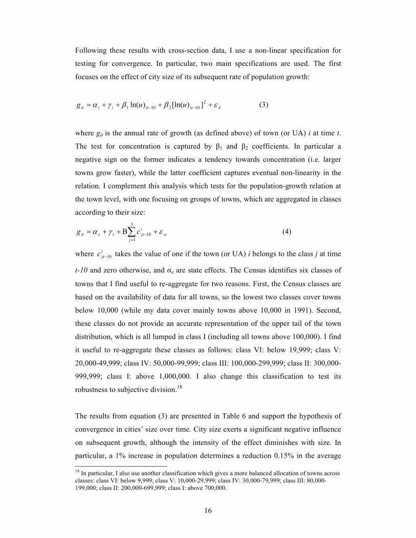
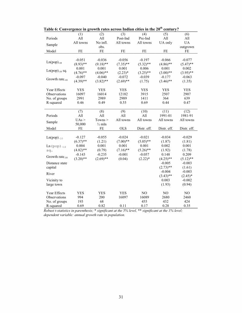
The results from equation (3) are presented in Table 6 and support the hypothesis of

convergence in cities’ size over time. City size exerts a significant negative influence

on subsequent growth, although the intensity of the effect diminishes with size. In

particular, a 1% increase in population determines a reduction 0.15% in the average

18 In particular, I also use another classification which gives a more balanced allocation of towns across

classes: class VI: below 9,999; class V: 10,000-29,999; class IV: 30,000-79,999; class III: 80,000-

199,000; class II: 200,000-699,999; class I: above 700,000.

17

annual rate of growth of (from the average value of 2.1% - column 1). These results

are robust to the exclusion of influential observations (column 2)19 and they are valid

for both the pre- and pos-Independence periods (columns 3-4). The results hold also

when considering only UAs (column 5), only towns belonging to UAs (column 6) and

only the larger UAs (over 50,000 – column 7). In the last three cases the inverse size-

growth relationship appears to be even more marked than in the baseline case. The

non-linearity seems to fade away for very large towns (over 500,000) – column 8. In

this case the negative effect appears to be linear.20

The main interpretation of these results is that as a town (or UA) grows in size, its rate

of growth slows down relative to the rate of growth experienced when its size was

smaller. This result is statistically more important than the cross-sectional one, i.e.

larger towns grow more slowly than smaller ones, as it is evident from two facts.

First, the FE regressions (in the first seven columns) explain a much larger part (by

over 100 times) of the within group than the between groups variation; second the

intensity of the size effect diminishes significantly in the OLS relative to the FE

estimation, as shown in column 9. However, the estimation without town effects

confirms the validity of the U-shaped relationship between growth and size, even

when I include district effects to control for local conditions likely to influence urban

growth (column 10).

This relationship is less evident at the cross-sectional level. It is valid but significant

only at the 5% level, when I regress the 1991-2001 annual growth rate on towns’ size

(including district effects and geographical controls) – column 11. And the

significance of the β coefficients disappears when I consider the 1991-2001 growth

rate (column 12), although the signs remain the same. The results from the last two

columns suggest that the strength of the growth convergence effect across towns may

not be as significant as that over time. The cross-sectional analysis further highlights

that the distance from the state capital negatively affects the town’s growth prospects,

and so does the presence of a navigable river.21 The negative coefficient on distance to

the state’s capital may have two non-mutually exclusive interpretations: it can indicate 19 I exclude those observations, for which the town either shrunk by more than 5% in any ten-year

period or grew by less more than 20%. 20 I regress the growth rate on the linear term, which is significant at the 1% level (not reported here).

21 This is a dummy variable which takes the value of 1 if the town has a navigable river.

18

the positive impact for a city’s prospects of being close to the seat of the political

power; it could also represent the effect of market potential on cities’ growth, as state

capitals are usually large markets as well. The latter effect is more clearly driving the

positive coefficient on the dummy for being situated within 20 kilometres from a large

town (over 100,000). The negative effect on a town’s growth prospects of being

situated by a river is more difficult to understand. It could be related to the physical

constraints to growth imposed by the presence of the river or to the danger of flooding

which may induce people to settle in towns without rivers. However, these

explanations would need further research to be verified. Thus geographical location

does seem to matter for cities’ growth in India, although further analysis would be

needed to draw more robust conclusions. Another significant finding is that there

seems to be no persistence in growth rates. The coefficient on past growth rate is

negative and significant in all FE specifications. On the other hand, the cross-sectional

analysis reveals a positive coefficient, which is in line with what found by Glaeser et

al. (1995) for a cross-section of US cities. This suggests that there is some sort of

mean reverting process in growth rates over time for individual cities, but persistence

does occur across the sample of cities (i.e. cities which have grown faster in the

previous decade continue to do so in the following one relative to the other cities).

Importantly, these reults are robust also to the inclusion of state-year effects, which

allow controlling for time varying state-specific urban systems.22 Calì (2007) argues

that Indian states could approximate national urban systems due to their vast size and

population as well as to their differences in terms of languages, culture and social

norms, which have limited the mobility of labour across states. Cashin and Sahay

(1995) find that the response of migration to income differentials across states was

similar to the weak responsiveness of population movements to income differentials

across the countries of Europe. Similarly, Topalova (2005) finds extremely limited

labour mobility across Indian regions between 1983 and 2000. Finally, the findings

are equally valid using a balanced panel, i.e. conditional on the existence and the

statistical reporting of towns in every year between 1951 and 2001.23

22 Results available from the author upon request.

23 This generates a sample of 1665 towns. Results of these regressions are available upon request.

19

The analysis using the classes of cities instead of the initial population confirms the

tendency of towns to slow down their growth as they become larger (Table 7). The

growth rate of towns is increasing in their class size. When a town becomes Class I

(i.e. the largest size), its rate of growth turns lower than when it was Class II, and so

on (column 1). This is the case also for UAs (column 2), and the results are robust to

using a different classification of towns as described above (column 3). Things change

when I include state effects but not town effects suggesting that town-level

characteristics are crucial in defining the size-growth relationship (column 4). A town

in class II (medium-large sized) is more likely to grow than any other town

(controlling for the state), while a town in class II (medium-small) is likely to grow

the least. Towns in class V (small towns) also grow slower, while the growth rates for

the other classes are not statistically different from towns in class III. These broad

results hold fairly well when considering only growth in 1991-2001 (column 5), but in

the 1981-1991 period class I towns have been the ones experiencing the lowest

growth (column 6). The results are unclear for the 1971-81 period (column 7) while

they indicate a bias against small towns in the pre-Independence period – column 8

(although this may just be the product of a classification which is less meaningful for

a period in which most towns would be classified in class VI and V). The

interpretation of these last results would require further scrutiny.

5. Conclusions

This paper has analysed three important aspects of the urbanisation process in India:

rural-urban disparities and their relation with economic development; the relation

between urbanisation and growth; and the convergence hypothesis in cities’ growth.

The results support the idea of a U-shaped relation between rural-urban disparities in

socio-economic indicators and the level of economic development. Such disparities

decrease as income per capita grows but at the diminishing rate until they reach a

trough and then there is some indication that they may start to rise again. This is the

mirror-image to the U-shaped inequality-income curve hypothesised by Kuznets

(1955). Dynamics in intra-rural and intra-urban inequalities may reconcile these rural-

urban results with national ones a la Kuznets.

20

I also found that although the level of urbanisation and that of economic development

go hand in hand across Indian states over time, this relation is not a very strong one.

On the other hand, it emerges quite clearly that the rate of urbanisation (i.e. how fast a

state urbanises) and the rate of growth appear to be negatively correlated. This finding

is somewhat surprising: in the ‘average’ Indian state, periods of faster urbanisation

tend to be associated with periods of slower growth. This may be related to

urbanisation patterns driven by push rather than pull factors, which are not favourable

to growth if not accompanied by the required investments in the urban sector.

Finally using a large dataset of Indian towns for the 20th century, the analysis has

shown that there is an important tendency towards convergence in growth rates

among Indian towns across all decades of the century. Other things being equal

smaller towns grow faster than large ones. This somewhat contrasts the fears of urban

concentration with large towns growing too quickly.

21

References

Au, C-C, and V.J. Henderson (2006). Are Chinese cities too small?, Review of

Economic Studies 73, pp. 549–76.

Barro, R. (1991). Economic growth in a cross-section of countries, Quarterly Journal

of Economics CVI, pp. 407-44.

Baumol, W.J. (1986). Productivity growth, convergence and welfare: what doe the

long-run data show?, American Economic Review 76, pp. 1072-85.

Bourguignon, F. and Morrisson, C. (1998). Inequality and Development: The Role of

Dualism, Journal of Development Economics, Vol. 57(2), pp. 233-257.

Calì, M. (2007). The agricultural sector and urbanisation patterns: Some evidence

from Indian states, London School of Economics, processed.

Cashin P. and R. Sahay, (1996). Internal Migration, Center-State Grants and

Economic Growth in the States of India, IMF Working Paper 95/58.

CIA (2003). The World Factbook 2002.

Combes P.P., G. Duranton and H.G. Overman (2005). Agglomeration and the

adjustment of the spatial economy, Papers in Regional Science, 84(3), pp. 311-49.

da Mata, D., Deichmann, U., Henderson, J.V., Lall, S.V. and H.G. Wang, (2007).

Determinants of city growth in Brazil, Journal of Urban Economics 62(2), pp. 252-

272.

Datt, G., (1995). Poverty in India 1951-1992: Trends and Decompositions, Policy

Research Department, World Bank, Washington, mimeo.

Davis, J. and J.V. Henderson (2003). Evidence on the Political Economy of the

Urbanization Process, Journal of Urban Economics, 53, 98-125.

Frankema, E. (2006). A Theil decomposition of Latin American income distribution

in the 20th Century: Inverting the Kuznets curve?, processed, University of Groningen.

Glaeser, E.L., J.A., Scheinkman, and A. Shleifer (1995). Economic growth in a cross-

section of cities, Journal of Monetary Economics, 36(1), pp. 117-43.

Government of India, various years. Statistical Census of India, 1951, 1961, 1971,

1981, 1991, 2001.

Henderson V.J. (2004). Urbanization and growth, Brown University, mimeo.

Kanbur, R. and X. Zhang (1999). Which Regional Inequality? The Evolution of

Rural–Urban and Inland–Coastal Inequality in China from 1983 to 1995, Journal of

Comparative Economics 27, pp. 686-701.

22

Kuznets, S., (1955). Economic Growth and Income Inequality, American Economic

Review, 1, Vol. XLV.

Lall S.V., H. Selod, and Z. Shalizi, (2006). Rural-urban migration in developing

countries: A survey of theoretical predictions and empirical findings. Policy

ResearchWorking Paper 3915,World Bank.

Lucas, R.E. (1990), \Why doesn't Capital Flow from Rich to Poor Countries?

American Economic Review Papers and Proceedings 80, 92-96.

Ozler, Datt and Ravallion, (1996). A Database on Poverty and Growth in India,

Washington: World Bank.

Planning Commission, (1993). Report on the Expert Group on the Estimation of the

Proportion and Number of Poor, Delhi: Government of India.

Qua, D. (1996). Empirics for economic growth and convergence, European Economic

Review 40(6), pp. 1353-75.

Topalova, P., (2005). Trade Liberalization, Poverty, and Inequality: Evidence from

Indian Districts, NBER Working Paper No. W11614.

23

Figures and Tables

Figure 1: Rural-urban disparities (headcount index) and GDP per capita across Indian states in the post-independence period

-1001020

-200204060

010203040

-5051015

-20020

-100102030

-100102030

-1001020

-1001020

010203040

-1001020

-10010

-2002040

-100102030

-20-10010

010203040

510

15

20

810

12

14

16

45

67

85

10

15

20

25

10

15

20

25

30

68

10

12

14

10

15

20

25

510

15

20

510

15

10

15

20

25

68

10

12

10

20

30

40

510

15

510

15

20

25

68

10

12

10

15

20

25

Andhra Pradesh

Assam

Bihar

Gujarat

Haryana

Jammu & Kashmir

Karnataka

Kerala

Madhya Pradesh

Maharashtra

Orissa

Punjab

Rajasthan

Tamil Nadu

Uttar Pradesh

West Bengal

Rural-urban poverty difference

GDP per capita

Note: Pover

ty diffe

rence

is meas

ure

d as the diffe

rence

between

the pover

ty hea

dcount in

dex in rura

l area

s an

d that in urb

an are

as

24

Figure 2: Rural-urban disparities (Mean consumption) and GDP per capita across Indian states, 1958-1994

11.21.41.6

1.522.53

11.21.41.61.8

11.21.41.6

11.21.41.6

11.522.5

11.21.41.61.8

1.21.41.61.8

.811.21.41.6

11.52

.6.811.2

1.11.21.31.41.5

11.52

11.522.5

.811.21.4

11.52

810

12

14

810

12

14

45

67

85

10

15

20

10

15

20

25

68

10

12

14

810

12

14

16

68

10

12

14

68

10

12

10

15

20

510

10

15

20

25

30

68

10

12

510

15

68

10

12

10

12

14

16

Andhra Pradesh

Assam

Bihar

Gujarat

Haryana

Jammu & Kashmir

Karnataka

Kerala

Madhya Pradesh

Maharashtra

Orissa

Punjab

Rajasthan

Tamil Nadu

Uttar Pradesh

West Bengal

Mean ratio

GDP per capita

25

Figure 3: Rural-urban death rates disparities and GDP per capita across Indian states, 1971-2001

2468

246810

2468

0246

02468

2468

2468

.2.4.6.81

246810

3456

468

1234

2468

246810

051015

0246

10

15

20

25

810

12

14

16

56

78

95

10

15

20

25

10

20

30

40

810

12

14

10

15

20

25

510

15

20

25

68

10

12

14

10

15

20

25

30

510

15

10

20

30

40

510

15

010

20

30

68

10

12

10

15

20

25

Andhra Pradesh

Assam

Bihar

Gujarat

Haryana

Jammu & Kashmir

Karnataka

Kerala

Madhya Pradesh

Maharashtra

Orissa

Punjab

Rajasthan

Tamil Nadu

Uttar Pradesh

West Bengal

Rural-urban death rate difference

GDP per capita

26

Figure 4: Evolution of rural-urban disparities and real income across Indian states over time, 1958-2002

510152025

810121416

456789

510152025

101520253035

68101214

510152025

510152025

68101214

1015202530

51015

10203040

6810121416

51015202530

681012

10152025

-1001020

-200204060

010203040

-5051015

-20020

-100102030

-100102030

-1001020

-1001020

010203040

-1001020

-10010

-2002040

-100102030

-20-10010

010203040

1960

1970

1980

1990

2000

1960

1970

1980

1990

2000

1960

1970

1980

1990

2000

1960

1970

1980

1990

2000

1960

1970

1980

1990

2000

1960

1970

1980

1990

2000

1960

1970

1980

1990

2000

1960

1970

1980

1990

2000

1960

1970

1980

1990

2000

1960

1970

1980

1990

2000

1960

1970

1980

1990

2000

1960

1970

1980

1990

2000

1960

1970

1980

1990

2000

1960

1970

1980

1990

2000

1960

1970

1980

1990

2000

1960

1970

1980

1990

2000

Andhra Pradesh

Assam

Bihar

Gujarat

Haryana

Jammu & Kashmir

Karnataka

Kerala

Madhya Pradesh

Maharashtra

Orissa

Punjab

Rajasthan

Tamil Nadu

Uttar Pradesh

West Bengal

head_diff

gdpcap_real

Poverty difference & Income

Year

27

Figure 5: Poverty difference vs. GDP per capita in 4 groups of states - trend line

05

10

15

20

05

10

15

20

0 10 20 30 40 0 10 20 30 40

1-Leading 2-Upper-Middle

3-Lower-Middle 4-Lagging

Poverty difference

GDP per capita

Graphs by 1-leading state 4 - lagging (by mean_gdp)

Leading States: Punjab, Haryana, Maharashtra and Gujarat

Upper-Middle States: West Bengal, Tamil Nadu, Karnataka, Andhra Pradesh

Lower-Middle States: Jammu & Kashmir, Assam, Kerala and Rajasthan

Lagging States: Madhya Pradesh, Uttar Pradesh, Orissa and Bihar

28

Table 1: Summary statistics for the main variables

Head diff PG diff

Mean

ratio

Death

rate diff

Per capita

GDP (Rs)

Annual

GDP

growth

Mean 8.06 2.42 1.39 4.13 12.29 0.05

Std. Dev. 10.79 4.03 0.31 2.04 5.82 0.08

Min -21.14 -11.03 0.64 -3.90 4.44 -0.27

Max 50.06 14.73 3.08 12.30 39.27 0.43

Table 2: Rural-urban disparities and income per capita across Indian states, 1958-2002

(1) (2) (3) (4) (5) (6) (7) (8)

Head

diff

Head

diff

Head

diff

PG diff Mean

ratio

Death

diff.

Death

diff.

Death

diff.

-2.465 -2.090 -1.382 -0.567 -0.070 -0.698 0.109 -0.144 GDP pc

(4.54)** (3.75)** (2.65)** (1.81) (3.18)** (11.60)** (1.59) (1.69)

0.047 0.038 0.042 0.016 0.001 0.013 0.001 0.004 GDP sq.

(4.37)** (3.73)** (3.24)** (2.58)* (2.80)** (8.01)** (0.64) (2.39)*

6.820 8.733 5.406 2.902 0.165 2.805 0.379 1.270 GDP growth

(1.76) (2.44)* (1.76) (1.73) (1.52) (4.04)** (0.53) (1.69)

-0.549 -1.306 -0.613 0.004 Rural 15-59

(1.57) (3.68)** (4.40)** (0.36)

0.561 0.418 0.164 0.013 Urban 15-59

(3.65)** (2.78)** (2.12)* (2.89)**

2.362 1.499 1.311 0.019 0.424 Rural 60+

(1.70) (1.06) (2.01)* (0.45) (1.87)

-5.287 -3.674 -1.336 -0.103 -0.991 Urban 60+

(2.90)** (2.18)* (1.45) (1.92) (3.77)**

-30.806 -8.449 3.363 1.874 -9.680 Fem/male

(15-34 rur) (1.10) (0.29) (0.25) (1.88) (2.13)*

1.023 1.105 -7.112 -0.485 -0.266 Ln pop.

(0.08) (0.28) (1.05) (1.19) (0.11)

-0.465 Rural 0-14

(6.60)**

-0.036 Urban 0-14

(1.40)

17.936 Urban share

(2.48)*

-0.414 GDP*1992

(1.67)

16.504 1992

(4.14)**

Year effects YES YES NO YES YES NO YES YES

State effects YES YES YES YES YES YES YES YES

Observations 564 522 522 462 462 448 448 403

R-squared 0.64 0.71 0.68 0.68 0.79 0.64 0.81 0.86

Robust t-statistics in parenthesis; * significant at the 5% level; ** significant at the 1% level.

29

Table 3: Economic growth and urban growth across Indian states, 1961-2001

(1

) (2

) (3

) (4

) (5

) (6

) (7

) (8

) (9

)

Ln G

DP

Ln G

DP

Ln G

DP

∆GDP

∆GDP

Ln G

DP

Ln G

DP

Ln G

DP

Ln G

DP

FE

FE

GLS A

R(1

) FE

GLS A

R(1

) FE

FE

FE

FE

Ln(G

DP

-1)

0.986

0.765

0.958

-0.242

-0.036

0.920

0.748

(1

4.40)*

*

(9.24)*

*

(59.57)*

*

(2.81)*

*

(1.98)*

(1

2.56)*

*

(9.01)*

*

Urb

an gro

wth

-1.261

-0.895

-0.963

-0.876

-0.861

(1

.38)

(1.09)

(2.27)*

(1

.03)

(1.66)

Ln urb

an p

op

-0

.075

-0.070

(0.70)

(0.73)

Urb

an shar

e

2.418

0.965

(2.76)*

*

(1.35)

Shar

e 60+

-0

.154

-0.176

-0.169

-0.113

-0

.156

-0

.082

(1.43)

(3.56)*

*

(1.50)

(1.84)

(1

.43)

(0

.46)

Shar

e 60+ sq.

0.015

0.014

0.016

0.010

0.015

0.014

(2.05)*

(3

.89)*

*

(2.10)*

(2

.16)*

(2.05)*

(1.19)

Ln tot pop

0.049

-0.025

0.051

-0.029

-0.303

0.028

0.011

(0.31)

(3.02)*

*

(0.30)

(3.18)*

*

(1.97)

(0.18)

(0

.04)

-0

.197

-0.172

-0.251

-0.087

-0

.164

0.718

Fem/m

ale (1

5-

34 rura

l)

(0

.52)

(2.08)*

(0

.64)

(0.98)

(0

.43)

(1

.16)

1971

-0.025

-0.038

-0.019

-0.035

-0.019

0.062

-0.014

0.013

0.008

(0

.98)

(0.90)

(1.55)

(0.81)

(1.17)

(1.21)

(0.26)

(0.26)

(0.11)

1981

0.014

0.004

0.024

0.008

0.022

0.199

0.057

0.096

0.092

(0

.46)

(0.05)

(1.58)

(0.10)

(1.11)

(1.99)

(0.58)

(1.45)

(0.64)

1991

-0.024

0.001

-0.002

0.005

0.006

0.276

0.093

0.286

0.290

(0

.57)

(0.01)

(0.11)

(0.04)

(0.27)

(1.83)

(0.64)

(3.46)*

*

(1.37)

2001

0.017

0.087

0.042

0.092

0.049

0.415

0.213

0.567

0.604

(0

.28)

(0.56)

(1.89)

(0.56)

(1.96)*

(2

.11)*

(1

.11)

(5.46)*

*

(2.24)*

Obse

rvatio

ns

76

70

70

70

70

76

70

76

70

Num

ber

of state

16

15

15

15

15

16

15

16

15

R-squar

ed

0.97

0.98

0.43

0.98

0.98

0.89

0.95

Robust t-statistics in parenthesis; * significant at the 5% level, ** significant at the 1% level; Jammu is the state excluded in the columns with demographic

variables, as data are not available.

30

Table 4: Summary statistics for cities’ population and population growth, 1901-2001

Population Growth rate

Obs. Mean Std. Dev. Obs. Mean Std. Dev.

1901 1,445 22,661 67,757

1911 1,487 23,148 76,908 1,390 -0.17% 2.93%

1921 1,580 23,357 80,792 1,462 0.38% 2.53%

1931 1,716 25,739 86,651 1,561 1.41% 2.04%

1941 1,893 31,975 128,275 1,703 1.88% 2.32%

1951 2,213 39,025 173,995 1,861 2.21% 3.00%

1961 2,382 48,829 222,716 2,003 2.49% 2.91%

1971 2,762 59,226 284,855 2,369 2.86% 2.54%

1981 3,294 71,098 357,531 2,714 3.27% 2.27%

1991a 4,428 72,771 402,377 3,287 2.75% 2.56%

2001b 3,943 96,539 544,474 3,936 2.17% 2.17%

a. The mean value for 1991 is not strictly comparable to that of the other years due to the wider cities’

coverage; b. the distribution of town for the year 2000 is slightly skewed towards larger towns due to

data availability.

Table 5: The effects of population size on subsequent growth, cross section (1) (2) (3) (4) (5) (6)

Periods 1991-2001 1991-2001 1981-91 1981-91 1971-81 1971-81

Ln(pop)-10 0.0012 -0.021 -0.019 -0.025 -0.016 -0.049

(0.25) (2.38)* (2.24)* (1.25) (1.57) (1.77)

Ln(pop)-10 sq. 0.0010 0.0011 0.0023

(2.46) (1.19) (1.78)

Observations 3818 3818 3029 3029 2460 2460

Dist. effects YES YES YES YES YES YES

Geo. controls YES YES YES YES YES YES

Adj. R-sq. 0.11 0.11 0.17 0.18 0.10 0.13

Robust t-statistics in parenthesis; * significant at the 5% level, ** significant at the 1% level

31

Table 6: Convergence in growth rates across Indian cities in the 20th century?

(1) (2) (3) (4) (5) (6)

Periods All All Post-Ind Pre-Ind All All

Sample All towns No infl.

obs.

All towns All towns UA only UA

outgrown

Model FE FE FE FE FE FE

-0.051 -0.036 -0.056 -0.197 -0.066 -0.077 Ln(pop)-10 (8.93)** (9.18)** (7.35)** (5.32)** (4.86)** (5.47)**

0.001 0.001 0.001 0.006 0.001 0.002 Ln(pop)-10 sq. (4.76)** (4.06)** (2.23)* (3.25)** (3.00)** (3.95)**

-0.097 -0.040 -0.072 -0.039 -0.177 -0.063 Growth rate-10 (4.39)** (3.82)** (2.69)** (1.75) (3.46)** (1.35)

Year Effects YES YES YES YES YES YES

Observations 16097 16014 12182 3915 2507 2907

No. of groups 2991 2989 2989 1411 364 639

R-squared 0.46 0.49 0.55 0.69 0.44 0.47

(7) (8) (9) (10) (11) (12)

Periods All All All All 1991-01 1981-91

Sample UAs >

50,000

Towns >

½ mln

All towns All towns All towns All towns

Model FE FE OLS Distr. eff. Distr. eff. Distr. eff.

-0.127 -0.055 -0.024 -0.021 -0.034 -0.029 Ln(pop)-10 (6.37)** (1.21) (7.00)** (5.05)** (1.87) (1.81)

0.004 0.001 0.001 0.001 0.002 0.001 Ln(pop)-10

sq. (4.82)** (0.79) (7.16)** (5.26)** (1.92) (1.78)

-0.143 -0.235 -0.001 -0.057 0.148 0.209 Growth rate-10 (3.20)** (2.69)** (0.04) (2.22)* (4.25)** (5.12)**

-0.005 -0.003 Distance state

capital (2.73)** (1.61)

-0.004 -0.003 River

(3.43)** (2.45)*

0.003 -0.002 Vicinity to

large town (1.93) (0.94)

Year Effects YES YES YES NO NO NO

Observations 994 200 16097 16089 2680 2460

No. of groups 193 68 455 432 424

R-squared 0.69 0.82 0.11 0.17 0.28 0.35

Robust t-statistics in parenthesis; * significant at the 5% level, ** significant at the 1% level;

dependent variable: annual growth rate in population.

32

Table 7: Class city size and population growth across size classes, 1901-2001

(1) (2) (3) (4) (5) (6) (7) (8)

Periods All All All All 2001 1991 1981 Pre-Ind

Sample Towns UAs Towns Towns Towns Towns Towns Towns

Model FE FE FE (diff.

classif.)

State

effects

State

effects

State

effects

State

effects

State

effects

-0.017 -0.026 -0.021 0.000 0.004 -0.008 -0.001 0.003 Class 1

(4.99)** (4.99)** (7.68)** (0.05) (1.19) (1.71) (0.11) (0.33)

-0.008 -0.016 -0.008 0.003 0.005 0.006 -0.002 0.005 Class 2

(3.91)** (4.36)** (4.83)** (2.29)* (1.89) (2.23)* (0.73) (0.94)

0.008 0.012 0.014 -0.002 -0.002 -0.002 -0.001 -0.005 Class 4

(6.15)** (5.14)** (10.26)** (2.28)* (1.31) (1.42) (0.63) (1.92)

0.018 0.027 0.029 -0.002 -0.002 -0.000 -0.002 -0.004 Class 5

(11.37)** (6.20)** (14.86)** (2.15)* (1.57) (0.22) (1.03) (1.93)

0.030 0.043 0.043 -0.001 -0.002 0.002 -0.000 -0.005 Class 6

(14.31)** (6.30)** (15.95)** (1.15) (1.12) (1.59) (0.16) (2.81)**

Year effects YES YES YES YES NO NO NO YES

Observations 20526 2887 20526 20526 3845 3061 2490 5486

No of groups 4207 374 4207 31 27 31 30 23

R-squared 0.16 0.17 0.18 0.14 0.03 0.09 0.06 0.13

Robust t-statistics in parenthesis; * significant at the 5% level, ** significant at the 1% level; figures in

bold indicate significance at the 10% level; dependent variable: annual growth rate in town’s

population.

33

Appendix 1

Methodological note to the construction of poverty measures

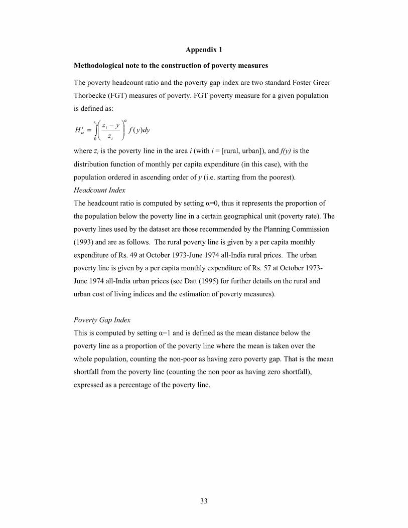
The poverty headcount ratio and the poverty gap index are two standard Foster Greer

Thorbecke (FGT) measures of poverty. FGT poverty measure for a given population

is defined as:

dyyfz

yzH

iz

i

ii )(0

∫

−=

α

α

where zi is the poverty line in the area i (with i = [rural, urban]), and f(y) is the

distribution function of monthly per capita expenditure (in this case), with the

population ordered in ascending order of y (i.e. starting from the poorest).

Headcount Index

The headcount ratio is computed by setting α=0, thus it represents the proportion of

the population below the poverty line in a certain geographical unit (poverty rate). The

poverty lines used by the dataset are those recommended by the Planning Commission

(1993) and are as follows. The rural poverty line is given by a per capita monthly

expenditure of Rs. 49 at October 1973-June 1974 all-India rural prices. The urban

poverty line is given by a per capita monthly expenditure of Rs. 57 at October 1973-

June 1974 all-India urban prices (see Datt (1995) for further details on the rural and

urban cost of living indices and the estimation of poverty measures).

Poverty Gap Index

This is computed by setting α=1 and is defined as the mean distance below the

poverty line as a proportion of the poverty line where the mean is taken over the

whole population, counting the non-poor as having zero poverty gap. That is the mean

shortfall from the poverty line (counting the non poor as having zero shortfall),

expressed as a percentage of the poverty line.

34

Appendix 2

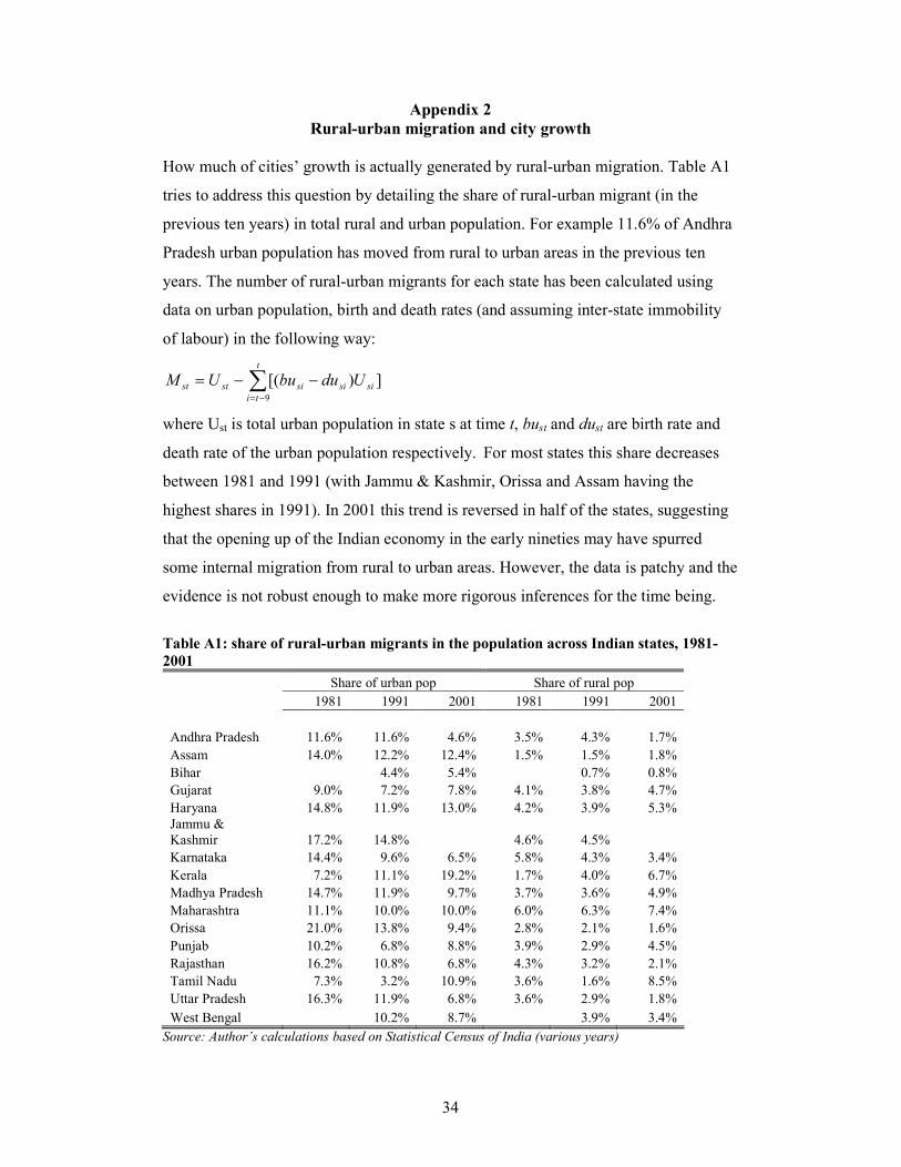
Rural-urban migration and city growth

How much of cities’ growth is actually generated by rural-urban migration. Table A1

tries to address this question by detailing the share of rural-urban migrant (in the

previous ten years) in total rural and urban population. For example 11.6% of Andhra

Pradesh urban population has moved from rural to urban areas in the previous ten

years. The number of rural-urban migrants for each state has been calculated using

data on urban population, birth and death rates (and assuming inter-state immobility

of labour) in the following way:

∑−=

−−=t

ti

sisisistst UdubuUM9

])[(

where Ust is total urban population in state s at time t, bust and dust are birth rate and

death rate of the urban population respectively. For most states this share decreases

between 1981 and 1991 (with Jammu & Kashmir, Orissa and Assam having the

highest shares in 1991). In 2001 this trend is reversed in half of the states, suggesting

that the opening up of the Indian economy in the early nineties may have spurred

some internal migration from rural to urban areas. However, the data is patchy and the

evidence is not robust enough to make more rigorous inferences for the time being.

Table A1: share of rural-urban migrants in the population across Indian states, 1981-

2001

Share of urban pop Share of rural pop

1981 1991 2001 1981 1991 2001

Andhra Pradesh 11.6% 11.6% 4.6% 3.5% 4.3% 1.7%

Assam 14.0% 12.2% 12.4% 1.5% 1.5% 1.8%

Bihar 4.4% 5.4% 0.7% 0.8%

Gujarat 9.0% 7.2% 7.8% 4.1% 3.8% 4.7%

Haryana 14.8% 11.9% 13.0% 4.2% 3.9% 5.3%

Jammu &

Kashmir 17.2% 14.8% 4.6% 4.5%

Karnataka 14.4% 9.6% 6.5% 5.8% 4.3% 3.4%

Kerala 7.2% 11.1% 19.2% 1.7% 4.0% 6.7%

Madhya Pradesh 14.7% 11.9% 9.7% 3.7% 3.6% 4.9%

Maharashtra 11.1% 10.0% 10.0% 6.0% 6.3% 7.4%

Orissa 21.0% 13.8% 9.4% 2.8% 2.1% 1.6%

Punjab 10.2% 6.8% 8.8% 3.9% 2.9% 4.5%

Rajasthan 16.2% 10.8% 6.8% 4.3% 3.2% 2.1%

Tamil Nadu 7.3% 3.2% 10.9% 3.6% 1.6% 8.5%

Uttar Pradesh 16.3% 11.9% 6.8% 3.6% 2.9% 1.8%

West Bengal 10.2% 8.7% 3.9% 3.4%

Source: Author’s calculations based on Statistical Census of India (various years)