Embed Size (px)
Citation preview

Linköping Studies in Science and Technology, Dissertations.No. 977
Uplink Load in CDMA Cellular RadioSystems
Erik Geijer Lundin
Department of Electrical EngineeringLinköpings universitet, SE–581 83 Linköping, Sweden
Linköping 2005

Uplink Load in CDMA Cellular Radio Systems
c© 2005 Erik Geijer Lundin
[email protected] of Automatic Control
Department of Electrical EngineeringLinköpings universitetSE–581 83 Linköping
Sweden
ISBN 91-85457-49-3 ISSN 0345-7524
Printed by LiU-Tryck, Linköping, Sweden 2005

To my sister and pärons!


Abstract
The uplink of code division multiple access (CDMA) cellularradio systems is often inter-ference limited. The interference originates from many users whose transmission powersare not observable for the system. This thesis introduces uplink load and applies means ofexplicitly considering the users’ radio environment when approximating and controllingthe load.
A desirable property of all cellular radio systems is uplinkfeasibility, i.e., existenceof finite user transmission powers to support the allocated services. Uplink load canbe considered as a measure of how far from infeasibility the system is. The performedcharacterization of uplink load lead to two concrete definitions related to the amount ofreceived and transmitted power, respectively.
An important part of the total load is the intercell load which is caused by users con-nected to neighboring base stations. If not carefully handled, the intercell load can jeop-ardize uplink feasibility. Conversely, knowledge of a lower intercell load can be used toincrease the resource assignments. A common denominator inall the work in this thesisis that the intercell load is explicitly considered.
When approximating uplink load, a centralized approach is adopted to study infor-mation gathered in several base stations. This yields good approximations of the averageload. However, centralized approximations can not detect momentarily peaks in the load.A number of resource allocation algorithms making control decisions in the local basestations are proposed based on experience from characterizing uplink load. As the al-gorithms study the intercell load, yet without measuring the interference power, they arerobust in the sense that they will never assign resources yielding an infeasible system.
A straightforward way of controlling the uplink load is to use measurements of thereceived interference power. This approach, just as the proposed load approximations, cangain from knowing the background noise power. The same framework used for designingrobust resource allocation algorithms, is also used for estimating the background noisepower.
v

vi

Acknowledgments
So these are the words of this thesis that will be read by the most people. The probabilityof me forgetting someone is certainly high, but I’ll give it ago anyway.
First of all, the man who I got to know when he helped me every Tuesday, the wholeday that is, during my master thesis, Dr. Fredrik Gunnarsson. Since then, he has excel-lently guided me through my time as a PhD student, without cutting down on those 20%of the work week. I am forever grateful for giving me exactly enough help to developboth my self and research results and never turning me down even when disturbing himat the Ericsson office. I don’t know how many times he has read half done work, which Iclaimed was ready for publishing.
Since I never moved out of the office room I was first placed in, Ihave had the pleasureof having Professor Fredrik Gustafsson next door ever sinceI joined the automatic controlgroup. This has made it easy for me to take advantage of his intuition and calm. He listens,even though it often does not look like it, and then proposes asimple solution to my, oftenpoorly formulated, question.
I like to take the opportunity to thank Professor Lennart Ljung for creating a goodworking atmosphere through good leadership. I also owe UllaSalaneck a thank you forcheerfully making all those administrative tasks work out smoothly.
The thesis has been proof read by Dr. Ragnar Wallin, Dr. Rickard Karlsson and DavidTörnqvist. Thank you for trying to make it readable even for those not already ensnaredinto the work. Gustaf Hendeby usually appears in acknowledgments for his TEX skills. Iwould like to thank him for more than just helping with the practical stuff. He has beena good friend and (LATEX-)companion during long weekends at the office. Without him,this thesis would not have happened as soon as it did.
Unfortunately, I will probably leave this place without repaying all the help I havereceived from people in the automatic control group. As has been concluded by manypeople before me, the group has a good atmosphere and everyone is willing to help.A thank you goes out to all the people in the group. There are some people who I havebothered also after office hours. These include Jonas Gillberg, who has been a good friendin tough situations, and Daniel Axehill with whom I have had rewarding discussions andreceived many good advice about boats of all kinds (they certainly helped during thoselong tedious periods away from the sea).
Dr. Gunnar Bark, Dr. Niclas Wiberg and Dr. Eva Englund are some of the peopleworking in the group at Ericsson, LinLab, that deserve a big thank you for being anendless source of inspiration and sharing their huge knowledge within radio resourcemanagement.
This project has been supported financially by the VINNOVA Center of ExcellenceISIS and the SSF graduate school ECSEL, which are gratefullyacknowledged. Ericssonhas provided both financial support and access to resources at their Linköping office whichis much appreciated.
A big thank you goes out to Ludde, Eva and Karin for the supportand hospitality theyhave shown without getting much in return. I would also like to thank Olle Berggren, theonly child hood friend I have left in the Swedish royal capital, for always having a placein his fishing boat despite me usually calling first during thelate Friday afternoon.
Linköping, November 2005Erik Geijer Lundin
vii


Contents
1 Introduction 11.1 Background and Objectives . . . . . . . . . . . . . . . . . . . . . . . . .11.2 Thesis Outline . . . . . . . . . . . . . . . . . . . . . . . . . . . . . . . . 21.3 Contributions and Publications . . . . . . . . . . . . . . . . . . . .. . . 4
2 Extended Summary 72.1 Cellular Radio Communication . . . . . . . . . . . . . . . . . . . . . .. 7
2.1.1 System Model . . . . . . . . . . . . . . . . . . . . . . . . . . . 72.1.2 Assumptions and Scope of the Thesis . . . . . . . . . . . . . . . 9
2.2 Characterizing Uplink Load . . . . . . . . . . . . . . . . . . . . . . . .102.3 Approximating Uplink Load . . . . . . . . . . . . . . . . . . . . . . . . 12
2.3.1 Derivation of Load Approximations . . . . . . . . . . . . . . . .132.3.2 Error Sources . . . . . . . . . . . . . . . . . . . . . . . . . . . . 142.3.3 Evaluation . . . . . . . . . . . . . . . . . . . . . . . . . . . . . 14
2.4 Analyzing Uplink Load . . . . . . . . . . . . . . . . . . . . . . . . . . . 152.5 Controlling Uplink Load . . . . . . . . . . . . . . . . . . . . . . . . . . 162.6 Feasibility versus Coverage . . . . . . . . . . . . . . . . . . . . . . .. . 192.7 Filtering and Estimating Uplink Load . . . . . . . . . . . . . . . .. . . 20
2.7.1 Noise Rise Relative Load Filtering . . . . . . . . . . . . . . . .. 202.7.2 Background Noise Power Estimation . . . . . . . . . . . . . . . 21
3 Cellular Radio Communication 253.1 Radio Wave Propagation . . . . . . . . . . . . . . . . . . . . . . . . . . 263.2 Radio Communication Systems . . . . . . . . . . . . . . . . . . . . . . .283.3 Multiple Access . . . . . . . . . . . . . . . . . . . . . . . . . . . . . . . 29
3.3.1 Orthogonal Signals . . . . . . . . . . . . . . . . . . . . . . . . . 293.3.2 Nonorthogonal Signals . . . . . . . . . . . . . . . . . . . . . . . 29
ix

x Contents
3.4 Cellular Radio Networks . . . . . . . . . . . . . . . . . . . . . . . . . . 303.5 System Performance . . . . . . . . . . . . . . . . . . . . . . . . . . . . 333.6 Radio Resource Management Algorithms . . . . . . . . . . . . . . .. . 34
3.6.1 Power Control . . . . . . . . . . . . . . . . . . . . . . . . . . . 343.6.2 Load Control . . . . . . . . . . . . . . . . . . . . . . . . . . . . 35
3.7 WCDMA . . . . . . . . . . . . . . . . . . . . . . . . . . . . . . . . . . 37
4 Characterizing Uplink Load 394.1 System Load and Capacity . . . . . . . . . . . . . . . . . . . . . . . . . 404.2 Decentralized Load . . . . . . . . . . . . . . . . . . . . . . . . . . . . . 43
4.2.1 Intercell-to-Intracell-Interference Factor . . . . .. . . . . . . . . 444.2.2 Interference Power Measurements . . . . . . . . . . . . . . . . .45
4.3 Centralized Load . . . . . . . . . . . . . . . . . . . . . . . . . . . . . . 454.3.1 Feasibility Relative Load . . . . . . . . . . . . . . . . . . . . . . 464.3.2 Convergence of Power Control Algorithms . . . . . . . . . . .. 484.3.3 Link Based Estimates . . . . . . . . . . . . . . . . . . . . . . . . 50
4.4 Discussion . . . . . . . . . . . . . . . . . . . . . . . . . . . . . . . . . . 52
5 Approximating Uplink Load 535.1 Uplink Interference Power Expressions . . . . . . . . . . . . . .. . . . 535.2 Uplink Load Expressions . . . . . . . . . . . . . . . . . . . . . . . . . . 55
5.2.1 Methods for Solving Nonlinear Equations . . . . . . . . . . .. . 565.2.2 Approximation I: Equal Interference Power In All Cells . . . . . 565.2.3 Approximation II: Equal Background Noise Power . . . . .. . . 585.2.4 Approximation III: Distributed Information . . . . . . .. . . . . 605.2.5 Required Information . . . . . . . . . . . . . . . . . . . . . . . . 61
5.3 Comparison of the Uplink Load Expressions . . . . . . . . . . . .. . . . 625.4 Sources of Estimation Errors . . . . . . . . . . . . . . . . . . . . . . .. 63
5.4.1 Nonlinear Relation Between CIR and CTIR . . . . . . . . . . . .635.4.2 TX Increase . . . . . . . . . . . . . . . . . . . . . . . . . . . . . 64
5.5 TX Increase Compensation . . . . . . . . . . . . . . . . . . . . . . . . . 655.6 Summary of Proposed Approximations and Compensation Methods . . . 675.7 Simulations . . . . . . . . . . . . . . . . . . . . . . . . . . . . . . . . . 68
5.7.1 Simulation Setup . . . . . . . . . . . . . . . . . . . . . . . . . . 685.7.2 Measurement Report Frequency . . . . . . . . . . . . . . . . . . 685.7.3 One Radio Network Controller . . . . . . . . . . . . . . . . . . . 705.7.4 Several Radio Network Controllers . . . . . . . . . . . . . . . .75
5.8 Summary . . . . . . . . . . . . . . . . . . . . . . . . . . . . . . . . . . 77
6 Analyzing Uplink Load 816.1 System Properties . . . . . . . . . . . . . . . . . . . . . . . . . . . . . . 82
6.1.1 Terminology . . . . . . . . . . . . . . . . . . . . . . . . . . . . 826.1.2 Interference Power Expression . . . . . . . . . . . . . . . . . . .83
6.2 System Load . . . . . . . . . . . . . . . . . . . . . . . . . . . . . . . . 846.2.1 System Noise Rise Relative Load . . . . . . . . . . . . . . . . . 846.2.2 Feasibility Relative Load . . . . . . . . . . . . . . . . . . . . . . 84

xi
6.3 Estabilishing the Feasibility Relative Load . . . . . . . . .. . . . . . . . 866.3.1 Connectivity One . . . . . . . . . . . . . . . . . . . . . . . . . . 866.3.2 Higher Connectivity . . . . . . . . . . . . . . . . . . . . . . . . 89
6.4 Relative Load Comparisons . . . . . . . . . . . . . . . . . . . . . . . . .906.4.1 Connectivity One . . . . . . . . . . . . . . . . . . . . . . . . . . 906.4.2 Higher Connectivity . . . . . . . . . . . . . . . . . . . . . . . . 92
6.5 Convergence of Fix Point Iterations . . . . . . . . . . . . . . . . .. . . 926.5.1 Connectivity One . . . . . . . . . . . . . . . . . . . . . . . . . . 936.5.2 Higher Connectivity . . . . . . . . . . . . . . . . . . . . . . . . 93
6.6 Approximating Uplink Load in Practice . . . . . . . . . . . . . . .. . . 936.7 A Simulation Example . . . . . . . . . . . . . . . . . . . . . . . . . . . 936.8 Summary . . . . . . . . . . . . . . . . . . . . . . . . . . . . . . . . . . 94
7 Controlling Uplink Load 977.1 Practical Centralized Resource Allocation . . . . . . . . . .. . . . . . . 987.2 Resource Control Approaches . . . . . . . . . . . . . . . . . . . . . . .1007.3 Resource Control Algorithms . . . . . . . . . . . . . . . . . . . . . . .. 102
7.3.1 Centralized Robust Algorithm . . . . . . . . . . . . . . . . . . . 1037.3.2 Semi-Centralized Robust Algorithm . . . . . . . . . . . . . . .. 1037.3.3 Decentralized Robust Algorithms . . . . . . . . . . . . . . . . .1077.3.4 Blind Algorithms . . . . . . . . . . . . . . . . . . . . . . . . . . 110
7.4 Resource Control Evaluations . . . . . . . . . . . . . . . . . . . . . .. 1117.5 Inaccurate Background Noise Power Knowledge . . . . . . . . .. . . . 1137.6 Summary . . . . . . . . . . . . . . . . . . . . . . . . . . . . . . . . . . 117
8 Feasibility versus Coverage 1198.1 Unlimited Transmission Powers . . . . . . . . . . . . . . . . . . . . .. 120
8.1.1 Two Users . . . . . . . . . . . . . . . . . . . . . . . . . . . . . 1208.1.2 Several Users . . . . . . . . . . . . . . . . . . . . . . . . . . . . 120
8.2 Limited Transmission Powers . . . . . . . . . . . . . . . . . . . . . . .. 1218.2.1 Link Budget . . . . . . . . . . . . . . . . . . . . . . . . . . . . 1218.2.2 Density Functions and Constants . . . . . . . . . . . . . . . . . .1228.2.3 Simulations . . . . . . . . . . . . . . . . . . . . . . . . . . . . . 123
8.3 Maximum Load . . . . . . . . . . . . . . . . . . . . . . . . . . . . . . . 1258.4 Summary . . . . . . . . . . . . . . . . . . . . . . . . . . . . . . . . . . 126
9 Filtering and Estimating Uplink Load 1299.1 Adaptive Filtering Theory . . . . . . . . . . . . . . . . . . . . . . . . .129
9.1.1 Kalman Filtering . . . . . . . . . . . . . . . . . . . . . . . . . . 1309.1.2 Linearized Kalman Filtering . . . . . . . . . . . . . . . . . . . . 1319.1.3 Extended Kalman Filtering . . . . . . . . . . . . . . . . . . . . . 1329.1.4 Particle Filtering . . . . . . . . . . . . . . . . . . . . . . . . . . 1329.1.5 Change Detection . . . . . . . . . . . . . . . . . . . . . . . . . . 133
9.2 Load Filtering . . . . . . . . . . . . . . . . . . . . . . . . . . . . . . . . 1359.2.1 Motivation . . . . . . . . . . . . . . . . . . . . . . . . . . . . . 1359.2.2 Signal Model . . . . . . . . . . . . . . . . . . . . . . . . . . . . 137

xii Contents
9.2.3 Design Choices . . . . . . . . . . . . . . . . . . . . . . . . . . . 1389.2.4 Simulations . . . . . . . . . . . . . . . . . . . . . . . . . . . . . 140
9.3 Background Noise Power Estimation . . . . . . . . . . . . . . . . . .. . 1409.3.1 Connectivity One . . . . . . . . . . . . . . . . . . . . . . . . . . 1429.3.2 Higher Connectivity . . . . . . . . . . . . . . . . . . . . . . . . 1439.3.3 Estimation Limitations . . . . . . . . . . . . . . . . . . . . . . . 1449.3.4 Simulations . . . . . . . . . . . . . . . . . . . . . . . . . . . . . 1469.3.5 Implementation Aspects . . . . . . . . . . . . . . . . . . . . . . 149
9.4 Summary . . . . . . . . . . . . . . . . . . . . . . . . . . . . . . . . . . 149
10 Conclusions 151
A Appendix 153A.1 Cellular Radio System Simulator . . . . . . . . . . . . . . . . . . . .. . 153
A.1.1 Models . . . . . . . . . . . . . . . . . . . . . . . . . . . . . . . 153A.1.2 Other Features . . . . . . . . . . . . . . . . . . . . . . . . . . . 154A.1.3 Simulator Utilization . . . . . . . . . . . . . . . . . . . . . . . . 154
A.2 Positive Matrices Theory . . . . . . . . . . . . . . . . . . . . . . . . . .154A.3 Schur Complement . . . . . . . . . . . . . . . . . . . . . . . . . . . . . 155A.4 Proof of Theorem 6.5 . . . . . . . . . . . . . . . . . . . . . . . . . . . . 156A.5 Proof of Theorem 6.7 . . . . . . . . . . . . . . . . . . . . . . . . . . . . 157A.6 Proof of Theorem 6.8 . . . . . . . . . . . . . . . . . . . . . . . . . . . . 157
A.6.1 Preliminaries . . . . . . . . . . . . . . . . . . . . . . . . . . . . 157A.6.2 Proof of Theorem 6.8 . . . . . . . . . . . . . . . . . . . . . . . . 159A.6.3 Standard Interference Functions . . . . . . . . . . . . . . . . .. 159
A.7 Proof of Lemma 7.2 . . . . . . . . . . . . . . . . . . . . . . . . . . . . . 160
Bibliography 161
Index 169

Notation
Symbols
B Number of base stations in the system, 30G Power gain matrix, 30Iother Intercell interference power, 43Iown Intracell interference power, 43Itot Total received interference power, 31K Link matrix, 82L System matrix, 83Lnr Noise rise relative load, 41Lf Feasibility relative load, 85Ls System noise rise relative load, 84M Number of users in the entire system, 30N Background noise power, 31Q Covariance matrix, process noise, 130R Covariance matrix, measurement noise, 130Z Relative power gain matrix, 83Λ Noise rise, 40α Propagation exponent, 26α Self interference factor, 32λ Eigenvalue with largest magnitude, 47β Carrier-to-Total-Interference Ratio (CTIR), 31βtgt Target CTIR, 42β0 Target CTIR in a single service system, 43ǫ Residual, 130γ Carrier-to-Interference Ratio (CIR), 31γtgt target CIR, 35
xiii

xiv Notation
x(t|τ) Estimate ofx(t) using data until timeτ , 130θ Background noise power ratio, 114λ Eigenvalue with smallest magnitude, 90f Intercell-to-intracell-interference factor, 44g Power gain, 26p Transmission power, 31q Shift operator,q−1x(t) = x(t − 1), 27x0 Linearization point, working point, 131
Abbreviations
CDMA Code Division Multiple Access, 29CIR Carrier-to-Interference Ratio, 28CTIR Carrier-to-Total-Interference Ratio, 31CUSUM CUmulative SUM, 134
EKF Extended Kalman Filter, 132
GoS Grade of Service, 33
LKF Linearized Kalman Filter, 131
PF Particle Filter, 132
QoS Quality of Service, 33
RMSE Root Mean Square Error, 146RNC Radio Network Controller, 37RRM Radio Resource Management, 34
SIR Signal-to-Interference Ratio, 28
WCDMA Wideband CDMA, 37

1Introduction
This chapter is meant to provide an overall picture of the rest of the thesis. After a briefdiscussion on the background and objectives of the work in the next section, the remainingchapters of the thesis are addressed one by one in Section 1.2. Main contributions andconcrete outcomes produced as the work progressed are summarized in Section 1.3.
1.1 Background and Objectives
Cellular radio systems providing speech service to users have been around long enoughto be a part of the every day living for a many people. The mobile phone is one of thethings you bring with you together with your wallet and keys as you walk on the street.Radio systems providing a multitude of services to the users, on the other hand, can notyet be called mature.
The radio resource management(RRM) problem can be defined as the problem ofdeciding what service to provide to each specific user. The increased complexity dueto a multitude of services in the radio systems of today makesthe RRM problem morechallenging. In the systems considered in this work, using an inadequate RRM algorithm,the algorithm solving the RRM problem, does not only correspond to inefficient resourceutilization, it can also mean that the ability to provide anyservice at all is jeopardized.
A fundamental criterion for a well operating RRM algorithm is accurate knowledgeof the amount of available resources, both currently and after a possible RRM decisionhas been made. The systems considered in this work usecode division multiple ac-cess(CDMA) as the scheme for sharing resources between users. Because of CDMAcharacteristics, the total amount of resources in the uplink, i.e., communication from mo-bile phone to the fixed base station, is not constant over time. Instead, it depends onwhere in the service area users are located. This makes it hard to decide how much of theresources that are currently used. Another word for this quantity, the ratio between used
1

2 1 Introduction
and total resources, isuplink relative load.The objectives of this work have been to characterize, approximate and control the
uplink load of a CDMA cellular system.
Characterizing Even though it is well known that the primary resource in the uplink isthe total received power, it is interesting to derive a measure of how far the system is frombeing overloaded. The first objective of this thesis is to provide definitions of uplink loadwhich can later be used in practice and/or theory.
Approximating A problem when trying to establish the uplink load in practice is thatit is hard to measure the received power accurately. Furthermore, the uplink load measureused in practice also involves the unknown background noisepower, which is why sim-ply using measurements of the uplink received power is not recommended. The secondobjective of this thesis is to derive practically attractive approximations of the uplink loadusing only readily available information.
Controlling The ability to provide service in one area covered by cellular radio systemdepends on decisions made in other areas. Thus, making inappropriate decisions in theown geographical area can ruin the possibilities to provideservices in the own area as wellas in other areas. This indicates that centralized control should be applied. On the otherhand, for increased performance, RRM decisions should be based on detailed informationon the local radio environment and momentarily transmission requests. Therefore, bothcentralized and decentralized schemes seem to have advantages. The third objective ofthis thesis is to develop robust and efficient RRM algorithmsbased on the knowledge andexperience gained from earlier parts of the thesis.
1.2 Thesis Outline
Below is a short explanation of the contents and purpose of the ten chapters in this thesis.Figure 1.1 provides an overview of where the chapters fit intoan automatic control viewof a cellular radio system.
Chapter 2 is a presentation of the results of the thesis. The chapter is, in terms ofdetails, intermediate between the ordinary abstract and the entire thesis. Basic knowledgeof cellular radio systems is here assumed to be known by the reader.
Chapter 3 provides fundamentals of systems for radio communicationsin general andCDMA cellular radio communications in particular along with the notation used through-out the thesis.
Chapter 4 introduces different aspects on uplink load in CDMA cellular radio systems.Uplink load from a practical point of view as well as from a more theoretical point ofview is given.

1.2 Thesis Outline 3
Load Control(Chapter 7) Power Control
System(Chapter 3)
γtgti
pi
External Disturbance
Power Gain Values
γi
Observer(Chapter 5)
ApproximativeLoad
Max Load(Chapter 8)
Figure 1.1: Resource control implemented as a cascade control system.
Once the uplink load is characterized, the remaining chapters contain the main resultsof this work. These results cover approximating and controlling the uplink load as wellas using the developed framework for advanced filtering techniques.
Chapter 5 contains the derivation of a number of load approximations suited for prac-tical use. Each approximation can be seen as an observer of the true system. The chapteralso contains simulation where the approximations are evaluated under rather realisticcircumstances.
Chapter 6 looks at relations between the load approximations derivedin Chapter 5 andmore theoretical aspects of uplink load. The analysis leadsto a method for guaranteeingconvergence of the uplink load approximations.
Chapter 7 uses experience from earlier chapters to design robust loadcontrolling algo-rithms. Included in the chapter is a simulation study to givean idea of the performance ofthe algorithms.
Chapter 8 looks at the uplink load’s role in the always present trade off between net-work performance and service quality for individual users.For a fixed maximum load,for example, higher bit rates can be given to fewer users, or coverage can be increased atthe expense of less momentarily revenue for the operator.
Chapter 9 contains two applications of signal processing. The purpose of the first ofthese is to provide a more stable load approximation, while the second application usesnonlinear filtering to estimate the background noise power based on readily availablemeasurements.
Chapter 10 contains the conclusions of the thesis.

4 1 Introduction
1.3 Contributions and Publications
The main contribution is the overall results on uplink load in CDMA cellular radio sys-tems. The results cover characterizing, approximating andcontrolling the uplink load.
Detailed contributions are:
• Development and evaluation of centralized load approximations in Chapter 5.
• The framework including the system matrix introduced in Chapter 6. Much of thetheoretical results are based on this framework.
• Development and evaluation of decentralized robust resource controlling schemesin Chapter 7.
Results presented in this thesis are partially covered by the following publications.
• The work on characterizing load in Chapter 4 is to a great extent also provided in
Erik Geijer Lundin and Fredrik Gunnarsson. Characterizinguplink load- concepts and algorithms. In Mohsen Guizani, editor,Wireless Com-munications Systems and Networks, chapter 14, pages 425–441. KluwerAcademic, 2003.
• The load approximations derived and evaluated in Chapter 5 were published in
Erik Geijer Lundin, Fredrik Gunnarsson, and Fredrik Gustafsson. Up-link load estimation in WCDMA. InProceedings of the IEEE WirelessCommunications and Networking Conference, New Orleans, LA, USA,March 2003c.
and
Erik Geijer Lundin, Fredrik Gunnarsson, and Fredrik Gustafsson. Up-link load estimates in WCDMA with different availability of measure-ments. InProceedings of the IEEE Vehicular Technology Conference,Cheju, South Korea, April 2003a.
• Schemes for controlling uplink load are defined and evaluated in Chapter 7. This isbased on
Erik Geijer Lundin, Fredrik Gunnarsson, and Fredrik Gustafsson. Ro-bust uplink resource allocation in CDMA cellular radio systems. InProceedings of the IEEE Conference on Decision and Control, Seville,Spain, December 2005a. To appear.
The work in Chapter 7 is based on the patent
Erik Geijer Lundin and Fredrik Gunnarsson. Using uplink relative pathgain related measurements to support uplink resource management. USPatent Application No: 11/066,558.

1.3 Contributions and Publications 5
• A part of Chapter 8 treats performance trade offs in the presence of limited trans-mission powers. This was first published in
Erik Geijer Lundin, Fredrik Gunnarsson, and Fredrik Gustafsson. Up-link load and link budget with stochastic noise rise levels in CDMAcellular systems. InRVK05, Linköping, Sweden, June 2005b.
• The adaptive filtering approach to load measure estimation in Chapter 9 was firstpublished in
Erik Geijer Lundin, Fredrik Gunnarsson, and Fredrik Gustafsson. Adap-tive filtering applied to an uplink load estimate in WCDMA. InProceed-ings of the IEEE Vehicular Technology Conference, Cheju, South Korea,April 2003b.
• A part of the work is summarized in
Erik Geijer Lundin and Fredrik Gunnarsson. Uplink load in CDMAcellular radio systems.IEEE Transactions on Vehicular Technology,2005. To Appear.
• Publications containing related work not included in this thesis are
David Törnqvist, Erik Geijer Lundin, Fredrik Gunnarsson, and FredrikGustafsson. Transmission timing - a control approach to distributed up-link scheduling in WCDMA. InProceedings of the American ControlConference, Boston, MA, USA, June 2004.
Fredrik Gunnarsson, Erik Geijer Lundin, Gunnar Bark, and Niclas Wiberg.Uplink admission control in WCDMA based on relative load estimates.In IEEE International Conference on Communications, New York, NY,USA, April 2002.

6 1 Introduction

2Extended Summary
The purpose of this chapter is to give a short version of the thesis, but yet elaborate onideas and results. No complete results are given here, only enough to give an idea ofwhat the corresponding parts of the thesis contain. As the sections in this chapter havethe same name as the remaining chapters, it is hopefully fairly easy to find more detailedderivations and results.
Section 2.1 introduces the notation used. Definitions of uplink load are made andmotivated in Section 2.2. Section 2.3 contains a short summary of the extensive work thathas been on deriving and evaluating a number of load approximations. The frameworkfor studying load from a more theoretical perspective and fundamental results are given inSection 2.4. Experience from Section 2.4 is then used in Section 2.5 to derive a number ofrobust algorithms for control of the uplink load. It is generally known that, for example,high load implies a tighter trade off between coverage, capacity and service quality forindividual users. Both a theoretical and a more practical aspect of this trade off is touchedupon in Section 2.6. Finally, signal processing is used in Section 2.7 to extract a morestable load approximation as well as estimating the background noise power.
2.1 Cellular Radio Communication
This section will only contain the introduced notation and is, unlike the correspondingchapter, not an attempt to introduce the reader to cellular radio communications in general.However, after having introduced the notation, the scope ofthe thesis is given from aautomatic control point of view.
2.1.1 System Model
Consider the uplink, i.e., communication from user to base station, of a code divisionmultiple access (CDMA) cellular radio system consisting ofM users andB base stations,
7

8 2 Extended Summary
or cells. The radio channel between useri and base stationj will simply be modeled asa power gain,gi,j < 1. Using this model, the received carrier power from useri in basestationj is
Ci,j = gi,jpi,
wherepi is the power useri transmits with.The limiting resource in the uplink of a CDMA cellular radio system is often thetotal
received interference power, Itot. The total received interference power in base stationjis modeled as the background noise power,Nj , plus the sum of received carrier powersfrom users on the same frequency band,
Itotj = Nj +
M∑
i=1
Ci,j , j = 1, 2, . . . , B. (2.1)
For the purpose of maintaining a suitable received signal quality, power control is imple-mented in the systems considered here. It is useful to introduce the following notation forthe base stations a user is power controlled by.
Definition 2.1 (Link Matrix). The element on rowi and columnj of the link matrix,K ∈ R
M×B , is defined as
Ki,j△
=
{
1, if useri is power controlled by base stationj
0, otherwise.
A similar quantity is the setKi which contains the base stations that useri is powercontrolled by, essentially
Ki△
= {j|Ki,j = 1}.The dual set is the set of users connected to a base station. For base stationj,
cj△
= {i|Ki,j = 1}.
The setsKi and power gain values are visualized in Figure 2.1. A user whois powercontrolled by several base stations, is said to be insoft handoverbetween these cells. Tocharacterize the number of cells a user may be power controlled by, the termconnectivityis introduced.
Definition 2.2 (Connectivity). A system is said to haveconnectivityk if at least oneuser is power controlled byk base stations.
In a system with connectivity one, each setKi, i = 1, 2, . . . ,M contains only onebase station. Uplink load is often related to uplinknoise risein the literature. The uplinknoise rise is defined as
Λj△
=Itotj
Nj.
The quality of the signal transmitted by useri and received in cellj is characterized bythecarrier-to-interference ratio(CIR),
γi,j△
=Ci,j
Itotj − Ci,j
.

2.1 Cellular Radio Communication 9
Ci,j Ci,k
Ci,ℓ
Received PowerReceived PowerReceived Power
Transmitted Powerpi
i
j kkℓ
Kigi,j
gi,k gi,ℓ
Figure 2.1: Variables in a cellular radio system.
For notational ease,carrier-to-total-interference ratio(CTIR), β, is introduced,
βi,j△
=Ci,j
Itotj
.
The relations betweenγ andβ are simply
β =γ
1 + γandγ =
β
1 − β.
The total perceived signal quality is related to the CIR and CTIR obtained by combiningthe signals received in different base stations. These total CIR and CTIR will simply bedenoted byγi andβi, respectively. For example, in case of connectivity one,
γi = γi,Kiandβi = βi,Ki
.
2.1.2 Assumptions and Scope of the Thesis
Communication systems are among the most complex systems built by man. As such,there is much to gain from breaking down the system into smaller subsystems, whichcan be handled relatively independently. Besides splitting the system into uplink anddownlink, mechanisms of the system operating on different time scales can be separated.
Systems operating on different time scales are often stumbled upon within automaticcontrol. The different time scales make the system well suited for a cascade control

10 2 Extended Summary
framework, as in Figure 1.1. In the inner loop, where fast updates are made, power controladjusts the users’ transmission powers on a time scale of milliseconds. The purpose ofthe power control loop is to adjust the transmission powers to maintain an experiencedCIR approximately equal to a target CIR, despite variationsin the radio environment andbackground noise. The power control can only succeed if the individual target CIR values,γtgt
i for each useri, are not set too high. The adjustment of the target CIR valuesis doneby a number of load controlling algorithms in the outer loop operating at a far slower ratethan the power control. It is customary to analyze the inner and outer loop of a cascadesystem independently, which is motivated by the considerable difference in time scale.When analyzing the outer loop, the inner loop is often assumedto operate perfectly onthe time scale that the outer loop operates on. This work is entirely devoted to the loadcontrol part. Motivated by the cascade control view, it is always assumed that the systemhas perfect power control when deriving the results.
2.2 Characterizing Uplink Load
Example 2.1 is meant to give an intuitive view of one of the twodefinitions of uplink loadthat will be made, the noise rise relative load.
Example 2.1: Interference Limited System
Consider a system consisting of just one base station, i.e.,B = 1. The total receivedinterference power is
Itot1 = N1 +
M∑
i=1
Ci,1 = N1 +M∑
i=1
βiItot1 ⇔
Λ1 =Itot1
N1=
1
1 −∑Mi=1 βi
. (2.2)
The nature ofItot1 implies that it should be positive. Thus, a basic requirement is
M∑
i=1
βi < 1. (2.3)
This puts a constraint on the maximum combined CTIR that the users can have, regardlessof how much transmission power they have available.
Because of the polynomial in the denominator of (2.2), this is often called the pole equa-tion (Holma and Toskala, 2000). The above example shows thatthe system’s ability toprovide service to the users is limited, despite access to infinite transmission powers. Thisis true also for a system consisting of several cells. A system with this property is calledan interference limited system.
Noise Rise Relative Load. Since the system is interference limited, a definition ofuplink load should be related to the received interference power. The most common

2.2 Characterizing Uplink Load 11
definition of uplink load found in the literature is
Lnr △
= 1 − N
I= 1 − 1
Λ.
The indexnr, which is an acronym for noise rise, has been added to separate this loadfrom the other type of load defined below. This type of load, which will be callednoiserise relative loadis especially used for practical applications in the literature. The def-inition is natural, considering that the uplink interference power is the primary uplinkresource. Note that a noise rise relative load of zero corresponds to a noise rise of one,i.e.,Itot = N .
When introducing this type of load, it is common to talk about the pole capacity.This is the capacity, in whatever measure used, of the systemwhen the noise rise relativeload reaches one. This is a theoretical capacity since a noise rise relative load of onecorresponds to infinite interference powers.
For the purpose of establishing the noise rise relative loadin practice, the total re-ceived interference power is often split into three parts. One being the background noiseand the other two are interference from users connected to the own base station,intra-cell interference, and interference from users connected to other base stations, intercellinterference,
Itot = N + Iown + Iother.
The intercell interference depends on where users are located in the system. Thismeans that also the system’s pole capacity depends on where users are located and howmany users there are in different cells. Thesoft capacityof a system can only be reachedif soft characteristics, such as received interference power or power gain values betweenusers and base stations, are studied in theradio resource management(RRM). So, for ex-ample, an RRM algorithm studying the system’shard capacity, as in for example countingthe number of users or measuring the throughput of the system, can not fully utilize thesystem’s resources.
A common way of approximating the uplink load is to use anintercell-to-intracellfactor, f . When doing so, the intercell interference is assumed to be a fraction f ofthe intracell interference,Iother = fIown. The uplink load in base stationj is thenapproximated by
Lnrj ≈ 1
1 − (1 + f)∑
i∈cjβtgt
i
.
The soft capacity of the system can not be achieved when usingthis method.There are several reasons for operating a system at lower load than one. Lower load
means lower noise rise. A high noise rise indicates a high total interference power, some-thing which can cause problems with coverage as the users have limited transmissionpowers. Another reason is that it is harder for the power control to operate satisfactoryat a high noise rise level. Loosely speaking, small changes in the radio environment orsmall changes by the load control algorithm in Figure 1.1 will make much higher impactat high noise rise levels, see Figure 2.2.
Feasibility Relative Load. The second type of studied uplink load is related to theexistence of finite transmission powers to support the service requested by the load con-trol. A system isfeasibleif it exists finite transmission powers to support the requested

12 2 Extended Summary
0 0.1 0.2 0.3 0.4 0.5 0.6 0.7 0.8 0.9 10
5
10
15
20
Noise Rise Relative Load,Lnr
Noi
seR
ise,Λ
=I
to
t
N[d
B]
∆Lnr
∆Lnr
∆Λ
∆Λ
Figure 2.2: The nonlinear relation between noise rise relative load,Lnr, and noiserise,Λ. Additional load,∆Lnr, gives different noise rise contribution,∆Λ, at dif-ferent load levels.
signal qualities (Zander, 1993). If that is not the case, thesystem is infeasible. The uplinkfeasibility relative loadis defined as one over the factor by which all users’ target CTIRcan be scaled by while maintaining a feasible system,
Lf△
= supµ{ 1
µ: µβtgt
i leads to a feasible system}.
From the definition, it is clear that a feasibility relative load less than one,Lf < 1,corresponds to a feasible system.
The noise rise relative load is related to the load in a specific base station while thefeasibility relative load is related to the entire system. Furthermore, the feasibility relativeload is more of a theoretical load, since it only applies as long as the users have transmis-sion powers enough to support their target CTIR values. The noise rise relative load, onthe other hand, is always applicable and much easier to establish in a general, practicalsystem. A more detailed comparison between the two load definitions is made in Chap-ter 6. It is concluded, for example, that as long as all users can maintain their target CIRin a system with connectivity one, the feasibility relativeload is lower than or equal to thenoise rise relative load, i.e.,Lf ≤ Lnr. Equality holds only in a single cell system.
2.3 Approximating Uplink Load
A major part of this work has been spent on deriving and evaluating the performance of anumber of uplink load approximations of the uplink noise rise relative load. Using onlyreadily available information on the users’ target CTIR values and the power gain betweenusers and base stations, they provide approximations that are for free in a sense since theydo not require any additional signaling.
Due to the intercell interference part of the total inteference power, the noise riserelative load in one base station depends on the situation inthe surrounding cells. This

2.3 Approximating Uplink Load 13
yields that an approximation in a base station using only local information can not con-sider the whole interference power explicitly. The proposed load approximations, on theother hand, use information gathered in several base stations and can therefore explicitlyconsider all contributions to the total received interference power.
2.3.1 Derivation of Load Approximations
Inspired by what is done inWideband CDMA(WCDMA), a system utilizing soft han-dover is studied in Chapter 5. A consequence of utilizing soft handover is that the setsKi
may contain several base stations. This makes the relation between the interference powerin different base stations quite complex. To exemplify, first approximate the combinationof signals received from one user in different cells with maximum ratio combining. Usingmaximum ratio combining implies that the CIR of the combinedsignal equals the sum ofthe separately received signals’ CIR, i.e.,
γi =∑
k∈Ki
γi,k.
By neglecting the power control errors, received CIR can be approximated with targetCIR. Finally, transforming CIR into CTIR and using the modelof total received interfer-ence power in (2.1) at timet yields
Itotj (t) = Nj(t)+
M∑
i=1
pi(t)gi,j(t) ≈ Nj(t)+
M∑
i=1
gi,j(t)βtgt
i (t)∑
k∈Ki
gi,k(t)Itot
k(t)
, j = 1, 2, . . . , B.
(2.4)An important property of the above equation is that it only contains variables that can beexpected to be known in a central node, i.e., the users’ target CTIR and measured powergain values, and the quantity that will be solved for,Itot
j (t), j = 1, 2, . . . , B.Considering that there is one equation like (2.4) in each base stationj, calculating
either the uplink noise rise,Itotj /Nj , or the uplink noise rise relative load involves solving
a system of nonlinear equations. Two methods for doing this are proposed in Chapter 5,one is based on linearization and the other uses fix point iterations.
Linearization. By approximatingItotk (t) with Itot
j (t) in (2.4), the uplink noise riserelative load in base stationj at timet can be approximated by
Llinj (t) =
M∑
i=1
βtgti (t)
gi,j(t)∑
k∈Kigi,k(t)
.
The indexlin has been added to emphasize the linearity in the users’ target CTIR. Thisexpression should be compared to (2.3), which relates to a single cell system. Since allusers in the system is considered byLlin
j , not only the load caused by users connectedto the own cell, but also the load caused by users connected toother base stations areexplicitly considered. There is thus no need for an intercell-to-intracell factor as is usuallythe case in the literature.

14 2 Extended Summary
Fix Point Iterations. The system of nonlinear equations defined by (2.4) can be solvedthrough fix point iterations. by approximating the background noise power in all basestations with a common, but yet unknown, background noise power, i.e.,Nj(t) ≈ N(t)for all j, the nonlinear equations can be approximately solved usingfix point iterations,as in Algorithm 2.1. The parameterN iter is the number of fix point iterations performedbefore each update. The analysis in Chapter 6 yields that Algorithm 2.1 converges to the
Algorithm 2.1
Let Λ(t, 0) = ΛNMRC(t − 1)Forn = 1 to N iter
For j = 1 to B
Let Λj(t, n) = 1 +∑M
i=1 βtgti (t)
gi,j(t)Pk∈Ki
gi,k(t)
Λk(t,n−1)
ΛNMRC(t) = Λ(t,N iter)
true noise rise if provided with accurate power gain values and applied in a system withconnectivity one.
As the approximations derived here,Llinj andΛNMRC
j , study the users’ relative powergain and all cells simultaneously, a resource management algorithm using these approxi-mations can in fact achieve the system’s soft capacity.
2.3.2 Error Sources
Besides the approximations made during the derivation, examples of the error sources thatappear in practice are the following.
• Inaccurate and incomplete knowledge of the power gain between users and basestations.
• Inaccurate assumption on how signals received in differentcells are combined.
• TX increase, which is the increase in average intercell interference power due tofast power control.
2.3.3 Evaluation
A rather complex simulator has been used to perform an extensive simulation study onthe performance of the uplink load approximations. Many weaknesses of a true system ismodeled, such as imperfect power control and sparsely sampled power gain reports thatdo not include all base stations. The results from this studyare reported in Chapter 5.The simulator models many characteristics of a true system such as fast fading, decodingability, soft handover and user mobility.
When deriving (2.4), which defines the system of nonlinear equations that is the basesfor the approximations, maximum ratio combining of the signals was assumed. Similarexpressions as (2.4) are derived by assuming selection combining1 or the actual mix of
1When combining signals using selection combining, the CIR of the combined signal is the maximum CIRof the separately received signals.

2.4 Analyzing Uplink Load 15
maximum ratio and selection combining that is used in the system. Applying fix pointiterations to these systems of nonlinear equations leads totwo more approximations ofthe uplink noise rise. These will be referred to asΛNSEL andΛNBOTH , respectively.Figure 2.3 shows the average error of the approximations with and without a compensa-tion for the TX increase contribution to the true noise rise.The compensation requiresknowledge of the characteristics of the specific channels. The simulations indicate that
1 2 3 4 5 6 7 8 9−1
0
1
2
3
4
Λ[dB]
mea
n(Λ
[dB
]−
Λ[d
B])
ΛNMRC
ΛNSEL
ΛNBOTH
ΛNMRC
ΛNSEL
ΛNBOTH
Figure 2.3: Error in noise rise with 64 kbps users. The dashed lines representsapproximations with the proposed compensation for TX increase.
it is possible to approximate the uplink load to within 1 dB for as high noise rise levelsas 8 or even 9 dB. Even though not shown here, the variance of individual approxima-tion errors is fairly small. The TX increase compensation comes with a slight increase invariation in the errors.
Similar results for the approximations using linearization in Section 2.3.1 are reportedon in Chapter 5.
2.4 Analyzing Uplink Load
Relations between noise rise relative load and feasibilityrelative load are derived in Chap-ter 6. These relations, together with relations to the uplink load approximations are alsofound in Chapter 6, are used to provide a criteria for system feasibility. The results aredivided into those applicable to a system with connectivityone, and those applicable tosystems with higher connectivity.
A basis for much of the work in Chapter 6 is a framework using a matrix expressionfor the total received interference powers in the base stations. In order to derive the matrix,consider a system with connectivity one. This means that (2.4) simplifies to
Itotj (t) = Nj(t) +
M∑
i=1
βtgti (t)
gi,j(t)
gi,Ki(t)
ItotKi
(t) = Nj(t) +
M∑
i=1
βtgti (t)zi,j(t)I
totKi
(t).

16 2 Extended Summary
Here,zi,j(t) is therelative power gainwhich is defined for any connectivity as
zi,j(t)△
=gi,j(t)
∑
k∈Kigi,k(t)
.
The duality betweenKi andck impliesKi = k, ∀i ∈ ck. The total interference power ina system with connectivity one can therefore be expressed as
Itotj (t) = Nj(t) +
B∑
k=1
∑
i∈ck
βtgti (t)zi,j(t)I
totKi
(t) = Nj(t) +
B∑
k=1
Lk,j(t)Itotk (t),
whereLk.j(t)
△
=∑
i∈ck
βtgti (t)zi,j(t), k, j = 1, 2, . . . , B. (2.5)
Each elementLk,j(t) can be interpreted as the load that users power controlled bybasestationk causes in base stationj at timet. Compiling allLk,j into a matrixL = [Lk,j ]yields thesystem matrix. A matrix expression for the total received interference inallbase stations in a system with connectivity one is thus
Itot = N + LT Itot.
This expression is used repeatedly in Chapter 6 to derive various results. For example,the feasibility relative load of a system with connectivityone is the maximum eigenvalueof the system matrix, i.e.,
Lf = λ(L),
whereλ(L) is the eigenvalue of the system matrixL with maximum magnitude.Other results found in Chapter 6 give several bounds on the uplink feasibility rela-
tive load, bounds that are possible to calculate before a resource management decision ismade. Feasibility relative load is also related to convergence of the fix point iterationsdescribed in Section 2.3.1. For example, it is shown that Algorithm 2.1 converges to thetrue noise rise vector in a feasible system with connectivity one. The results found inChapter 6 are summarized in a procedure for approximating uplink load of a system witharbitrary connectivity.
2.5 Controlling Uplink Load
Various properties of the system matrix, whose elements aregiven by (2.5), are combinedwith experience from the theoretical analysis to design resource allocation algorithms inChapter 7. More concrete, the proposed allocation algorithms are optimization problemsin which the constraints are inspired by the relations givenby the theoretical analysis. Theutilization function in these problems is the sum of maximumachievable rate normalizedwith the signal bandwidth (Wozencraft and Jacobs, 1965, page 520),
∑
i
log2(1 + γtgti ).
Essentially, two resource allocation algorithms are proposed. They both make resourceallocations in local nodes while maintaining system feasibility. Neither of the algorithmsrely on measurements of the uplink noise rise.

2.5 Controlling Uplink Load 17
Decentralized Algorithm. The first proposed algorithm does not use a central node atall. The algorithm is based on a result applicable to all square matrices,
λ(L) ≤ ||L||∞.
Since all elements ofL are positive, the matrix infinity norm is simply the maximum rowsum.
A single base station can control all elements of a row in the system matrixL. There-fore, if all base stations make resource assignments such that the corresponding row isless than some constantLtgt
f , so will the feasibility relative load,Lf , be. Obviously, by
choosingLtgtf less than one, this yields a method for guaranteeing system feasibility.
A result by Gantmacher (1974) states that a lower bound onλ(L) is given by theminimum row sum. Therefore, if all row sums equalLtgt
f , so doesLf .
The optimization problem solved in each base stationk at each time instantt is
maxβtgt
i(t)∈ck
∑
i∈ck
log2(1 + γi(t)) = −∑
i∈ck
log2(1 − βtgti (t))
s.t.
{∑
i∈ckβtgt
i (t)∑B
j=1 zi,j(t) ≤ Ltgtf
βmin ≤ βtgti (t) ≤ βmax,∀i ∈ ck.
Semi-Centralized Algorithm. The second proposed algorithm uses a central node todistribute resource pools to the base stations. Each base station then assigns resources tothe users connected to it. System feasibility is guaranteedthrough the use of a mutualagreement between the central node and the base stations.
The purpose of the central node is to distribute resource pools to the base stations.Typically, a base station with many users in it should receive a larger resource pool. Byfeeding back information on where in the radio environment the users are located, softcapacity can be studied in the central node just as it is in thebase stations. Feedingcomplete information on each users’ location would requiretoo much signaling. Theinformation send back from base stationk at timet is
Yk,j(t)△
=1
∑
i∈ckβtgt
i (t − 1)
∑
i∈ck
zi,j(t − 1)βtgti (t − 1) = Lk,j(t − 1), j = 1, 2, . . . , B.
Based on the information received from all the base stations, the central node compiles amatrix L = [Lk,j ], with
Lk,j = skYk,j(t).
The resource pools,sj(t), j = 1, 2, . . . , B, are given in the central node as the solution to

18 2 Extended Summary
the following optimization problem
maxs
B∑
j=1
sj(t)
s.t.
(
E L
LT Ltgtf
2E
)
� 0
Lk,j = sk(t)Yk,j(t), k, j = 1, 2, . . . , B
sk(t) =∑
i∈ckβtgt
i (t)
βmin ≤ βtgti (t) ≤ βmax, i = 1, 2, . . . ,M.
Here,E is the identity matrix. The matrix inequality will guarantee that the maximumeigenvalue ofL is less than or equal to the target feasibility relative load, Ltgt
f . Now, ifeach elementLk,j(t) in the system matrix is less than or equal to the corresponding ele-ment inL, the maximum eigenvalue ofL(t) will also be less thanLtgt
f . This requirementwill be guaranteed by the way resources are assigned in the local nodes (the base stations).Upon receiving the resource poolsk(t), the resource assignment made by local nodekwill be the solution to the following optimization problem
maxβtgt
i(t)∈ck
∑
i∈ck
log2(1 + γi(t)) = −∑
i∈ck
log2(1 − βtgti (t))
s.t.
{∑
i∈ckβtgt
i (t)zi,j(t) ≤ Yk,j(t)sk(t)∀j
βmin ≤ βtgti (t) ≤ βmax, ∀i ∈ ck.
After the base stations have assigned target CTIR values, they calculate new valuesYk,j(t+1) and send them back to the central node. Using this iterative procedure, repeat-edly solving the optimization problems in the different nodes, implies that the algorithmcan adapt to changes in the radio environment as well as to users moving between cells.
Simulations. For comparison, two additional algorithms are introduced.One is acen-tralized algorithmwith complete knowledge of the radio environment in the entire system.This algorithm is meant to give an idea of what can be achieved. The second algorithm in-troduced for comparison do not use a central node nor relative power gain values, and willtherefore be referred to as theblind algorithm. Using this algorithm, each base station hasa resource pool ofs0 which it shares evenly over users connected to it. Figure 2.4showsthe result of a simulation study in which a small part of the service area has a considerablyhigher user density. This implies that there is performanceto gain by moving resourcesbetween base stations.
According to Figure 2.4a, both of the proposed robust algorithms provide practicallyequal capacity as the completely centralized, while the blind algorithm gives significantlylower capacity. Figure 2.4b shows the relative success rateof the robust algorithms. Thesemi-centralized algorithm’s ability to distribute resources between base stations resultsin a higher success rate for low target load levels. For example, in this specific scenario,choosing the target feasibility relative load to 0.5 yieldsthat the semi-centralized algo-rithm succeeds in approximately 80% of the cases while the decentralized algorithm only

2.6 Feasibility versus Coverage 19
3 4 5 6 7 8 9 104
6
8
10
0.2 0.3 0.4 0.5 0.6 0.7 0.8 0.9 10
0.2
0.4
0.6
0.8
1
Maximum Noise Rise [dB]
Sys
tem
Cap
acity
P(s
ucce
ss)
Ltgtf
a)
b)
CentralizedSemi-CentralizedDecentralizedBlind
Figure 2.4: Comparison of radio resource management algorithms.βmin = −15 dB(γmin ≈ −15 dB), βmax = 0.5 (γmax = 1). 50 Monte Carlo simulations.
manages to find a solution in 20% of the cases. Considering higher offered load, thesesuccess rates would appear for a higher target feasibility relative load. The difference insuccess rates between the different algorithms is due to thesemi-centralized algorithm’sability to distribute resources between the local nodes.
As a conclusion, by studying the relative power gain it is possible to design decen-tralized algorithms that provide a throughput comparable to that given by a completelycentralized algorithm. This is done with considerably less, or no, signaling between localand central nodes, without neglecting the robustness in terms of guaranteed feasibility.Furthermore, since the algorithms use local nodes, they cantake advantage of local infor-mation on for example the radio environment.
2.6 Feasibility versus Coverage
Thus far, focus has been on approximating or controlling theuplink load. By using a fewexamples, the trade off between capacity, coverage and quality of service for individualusers is addressed in Chapter 8.
Assuming that the users have transmission powers to supporttheir service, the feasi-

20 2 Extended Summary
bility relative load in a single service scenario with two cells and one user in each is givenby (dropping the time index,t)
Lf = β0(1 +√
z1,2z2,1) ⇔√
z1,2z2,1 + 1 =Lf
β0,
whereβ0 is the target CTIR values for the only service provided. The right hand siderelation indicates a possible trade off between coverage, in terms of users’ relative powergain, and capacity in terms of the target CTIR. This shows that the coverage is limited ina multi cell scenario, even if the users have unlimited transmission powers. As isolatedcells correspond to zero relative power gain to other cells,better isolation between cells ina system yields better capacity or possible higher service quality for the users. A possiblelimit on the uplink noise rise is in this case arbitrary, since it is the feasibility requirementthat provides the limitations. In a scenario where the relative power gain values are small,it is primarily the target CTIR,β0, that is constrained. This is scenario is referred to as acapacity limited scenario.
Now consider limited transmission powers. In this case it isperhaps wise to choose alow noise rise target for the resource allocation algorithms, in order to not lose too muchcoverage. A stochastic approach to link budgets has been applied to calculate an approx-imative relation between target CTIR, coverage and grade ofservice in a few examplescenarios. Figure 2.5 shows the relation between maximum allowed noise rise relativeload and cell radius. It is clear that the noise rise relativeload that a system can cope within practice decreases fast as the cell radius grow, especially in system deployments withlarge cells. The actual numbers on the x-axis depend on the specific scenario studied,such as the background noise power and maximum user transmission power. The shadedarea is where the system can be expected to be capacity limited, as opposed to coveragelimited.
A conclusion of this analysis, is thus that the target load for the resource allocationalgorithms depends on the specific power gain distribution.In some scenarios, the targetload is set by coverage demands, while in others it is the feasibility requirement that givesthe maximum allowed load. The system may thus be coverage limited or capacity limited.Since the distribution depends on the specific system deployment such as the size of thecells and antenna characteristics, it can be changed to someextent by choosing a differentsystem deployment.
2.7 Filtering and Estimating Uplink Load
Signal processing techniques have been used in two different applications in Chapter 9.These two are here explained in separate subsections.
2.7.1 Noise Rise Relative Load Filtering
The noise rise relative load is constantly oscillating about a load level, as can be noticedin practice. If these oscillations can be canceled, resource management algorithms canbe more aggressive, leading to better resource allocation.An ordinaryauto-regressive(AR) signal model, describing oscillations with zero mean,was extended to abiased AR

2.7 Filtering and Estimating Uplink Load 21
0 200 400 600 800 1000 1200 1400 1600 18000
0.2
0.4
0.6
0.8
1
Noi
seR
ise
Rel
ativ
eLo
ad
Cell Radius [m]
β0 = −13β0 = −9.5Data
Figure 2.5: Relation between average noise rise relative load and cell radius whenthe users have a 95% probability of experiencing coverage. Two different targetCTIR values are considered. A simple model has also been fitted to data. The shadedarea represents situations where the system is capacity limited, as opposed to cover-age limited. Aβ0 of -9.5 dB approximately corresponds to a 384 kbps service andβ0 = −13 to a 144 kbps service.
model, describing oscillations around an arbitrary level.In the application, this level isconsidered time varying and it is the primary quantity to estimate.
The developed signal model, Kalman filtering and change detection are applied to asignal produced by the load approximations derived in Section 2.3. The result is a morestable load approximation which is alert to sudden changes in the load level as well asan estimate of the load levels derivative. Ordinary low passfiltering of the signal wouldeither be very slow to adapt to a new load level or not suppressthe oscillations to the sameextent as the Kalman filter. Figure 2.6 shows an example of howthe estimation quicklyadapts to a new load level, while simply low pass filtering theestimate results in slowadaptation to a new load level.
2.7.2 Background Noise Power Estimation
When using measurements of the uplink interference power forresource management,an inaccurate measure of the background noise power can leadto decreased performancein terms of capacity and coverage. Signal processing is usedto estimate the backgroundnoise power using only available measurements of the uplinkinterference power. A non-linear signal model based on the system matrix, describing the relation between back-ground noise power and measured received interference power, is developed. The modelincorporates uplink interference power measurements being corrupted by a base stationindividual bias in logarithmic scale.
As a nonlinear signal model is used, the estimation performance can be improved byusing nonlinear filtering. Besides linearizing the state space model and applying a Kalmanfilter, extended Kalman filter(EKF) and particle filters have been applied.
The EKF, in general, uses a linearized version of the nonlinear model where the lin-earization point is repeatedly chosen to the latest estimated state variables. The particle

22 2 Extended Summary
1250 1260 1270 1280 1290 1300 1310 1320 1330 1340 13500.4
0.45
0.5
Time [s]
Load
Figure 2.6: Example of estimated average load level when simply low passfiltering(dashed) and using a biased AR-model together with Kalman filtering and changedetection (solid thick). The thin solid line is the load approximation used as input tothe estimation process.
filter uses Monte Carlo integration to approximate the probability density function for thetrue state space vector. The main strength with particle filters is that almost arbitrary prob-ability density functions for the measurement and process noise can be modeled. Whenusing particle filters a nonlinear signal model does not haveto be linearized at any stage.
The application performs well, despite the rather unrealistic circumstances assumedduring the derivation. Even when soft handover is used in thesimulations, unlike in themodeling, the algorithm manages to estimate the backgroundnoise power with usuallyless than 1 dB error in bursty traffic. Figure 2.7 shows how an EKF and two differentparticle filters with 5000 and 10000 particles, respectively adapts to a sudden change inthe background noise power in one out of nine base stations. Using more particles impliesa better approximation of the probability density functionfor the possible values of thestate vector. However, in this case, 5000 particles seem to be enough to still detect thesudden change in the true background noise power.

2.7 Filtering and Estimating Uplink Load 23
0 10 20 30 40 50 600.4
0.6
0.8
1
1.2
1.4
1.6
1.8
Time [s]
TrueEKF
PF2PF1
Figure 2.7: Example of background noise power estimation. The true backgroundnoise power makes jumps att = 20 s andt = 40 s. The particle filters have 5000(PF1) and 10000 (PF2) particles. EKF is the extended Kalman filter. It is the productof background noise power and measurement bias on the y-axis.

24 2 Extended Summary

3Cellular Radio Communication
A requirement for applying math to wireless communication systems is obviously a wayof mathematically describing how a signal changes as it travels through the air. Since theexact behaviour of the propagation channel is far too complex to be described exactly, amodel is used. The first section of this chapter describes howthe propagation channel ismodeled. Besides the propagation channel, two other important parts of a radio systemare the transmitter and the receiver. Section 3.2 describesthe generic parts of these twocomponents.
For many reasons, one being that the bandwidth available forradio communication islimited and therefore expensive, the radio spectrum must beefficiently utilized. Methodsfor sharing the available bandwidth are presented in Section 3.3. Because of this sharing,users will interfere with each other. However, if they can bespatially separated, a user willshare the available bandwidth with less users. This is one ofthe ideas behind cellular ra-dio networks. Theory regarding cellular radio networks is further explored in Section 3.4.There is a number of expectations on a radio system. What theseexpectations are de-pends on what kind of relation you have with the system. An attempt to characterize theperformance of the system is done in Section 3.5. In order to utilize available resourcesin an efficient manner, radio resource management algorithms are used. In Section 3.6fundamental radio resource management algorithms are mentioned and their purpose ex-plained.
Exactly how these algorithms are implemented is a choice of the individual systemmanufacturers. However, successful operation over manufacture borders requires stan-dardization, both in terms of radio network architecture and in protocols between forexample transmitters and receivers. The last section of this chapter presents details ofthe architecture of a WCDMA system and, for the present work interesting, parts of thecurrent standard.
25

26 3 Cellular Radio Communication
3.1 Radio Wave Propagation
A signal propagating through the air is subject to attenuation. Given perfect knowledgeof the surrounding environment, this attenuation can be calculated using Maxwell’s equa-tions. This, of course, is not practically feasible for manyreasons. Therefore, a simplifiedversion of the reality, a model, is used. A criteria for the model is that it will provide astatistically correct description of the attenuation. Instead of modeling the attenuation, itsinverse,power gain, is often modeled. The received signal power can comprehensivelybe expressed as transmitted power times the power gain. The model is often separatedinto three components. The product of these three is the power gain
g = gpgsgmp < 1,
wheregp representspath gain1, gs shadow fadingandgmp multipath fading. These threecomponents are explained in a bit more detail below.
Path loss is the long term attenuation caused by the distance between transmitter andreceiver. Path loss is the dominating factor in for example satellite communications. It isusually modeled as
gp = Cpr−α, (3.1)
whereCp is a constant which depends on the gain at the receiving antenna and the wave-length of the radio signals,r is the distance between transmitter and receiver andα is aradio environment dependent,propagation exponentranging from 2 (free space propaga-tion close to the antenna) to5.5 (far from the antenna in a very dense urban environment).This model, with terrain dependentα andCp, was verified by Okumura et al. (1968)and Hata (1980). In cellular radio systems,α is usually taken equal to4 (Gilhousen et al.,1991).
Shadow fading is due to large obstacles in the radio environment, objects which mayabsorb the radio wave. This part of the power gain is not, unlike the path loss, strictlyincreasing with the distance. Shadow fading is usually modeled using a log-normal dis-tribution (Hata, 1980; Okumura et al., 1968)
gs = 10ξ/10, ξ ∈ N (0, σs).
This model assumes that the user is standing still and thus experiences the same shadowfading over time. A user moving around in the environment will experience time varyingshadow fading. The correlation between two consecutive samples of the shadow fadingdepends on how fast the user is moving. Gudmundson (1991) proposes a model wherethe correlation is expressed using a relation between the user’s speed,v, and acorrelationdistance, d0. This distance is chosen together with an additional constant ǫD such thatthe correlation between the shadow fading at two points separated a distanced0 should be
1The transmitting antenna’s gain and performance of the algorithms in the receiver can also be incorporatedin the path gain.

3.1 Radio Wave Propagation 27
ǫD. The dependence between consecutive samples is then implemented by filtering the
ξ-values through a first order low pass filter with a pole atǫvTd0
D
y(t) =(1 − ǫ
vTd0
D )q
q − ǫvTd0
D
ξ(t), gs = 10y/10.
The constantT is the sampling time used,t = 1, 2, . . . represents the discrete time instantsandq is the shift operator (e.g.,q−1ξ(t) = ξ(t − 1)).
Multipath fading is caused by signals being reflected on obstacles in the radioenvi-ronment. The reflections cause a signal to be received in several copies. Since thesecopies may arrive at different times and with different strength, they interfere either con-structively or destructively. Multipath fading depends onthe user’s position relative thesurrounding environment. Thus one position does not have a time constant multipath fad-ing due to a time varying radio environment. This contribution can change very rapidly,which is why it is also called fast fading. Further details onmulti path fading can befound in Sklar (1997). The changes in the multi path fading produces deep fades in thetotal power gain, but the multi path fading gain can occasionally be larger than 1 (0 dB).Multipath fading also causes local deep fades in the frequency spectrum. In case of narrow
0 0.5 1 1.5 2 2.5 3 3.5 4 4.5 5−10
−5
0
5
10
Distance [m]
g mp
[dB
]
Figure 3.1: Example of the multipath fading part of the total power gain after therake receiver, when adopting the characteristics given by 3GPP Typical Urban mul-tipath model, (3GPP, 2000c).
band communication this can be devastating.
One way of decreasing the variations in experienced power gain which the multipathfading causes is to use a rake receiver. A rake receiver estimates the relative delay ofseparate signal copies (rays). The information from different rays can then be combinedproviding a more stable total power gain after the rake receiver. Figure 3.1 illustrates themultipath fading gain after the rake receiver.

28 3 Cellular Radio Communication
3.2 Radio Communication Systems
Figure 3.2 shows the generic parts of a radio system. A message given to the sourceencoder can be in practically any format, such as a text file, apicture or speech. Thesource encoder converts this information into a string of bits.
These bits are then given to a channel encoder. A channel encoder adds redundancybits, which in the receiver will be used to correct errors induced between sender andreceiver. Both information bits and redundancy bits are then used to modulate a carriersignal. This process produces a high frequency signal whichis suited for transmissionover the air interface.
At the other end, on the receiver side, things are basically done in the opposite direc-tion. However, algorithms here are much more complicated. For example, demodulationusually requires accurate synchronization between receiver and sender. The channel de-coder uses the redundancy bits introduced by the channel encoder to detect and possiblycorrect bit errors. Finally, the source decoder converts the bits into the form of the orig-inal information. In order to provide a certain service to the users, the system has to
SourceEncoder
ChannelEncoder Modulation
DemodulationChannelDecoder
SourceDecoder
SIR CIR
Message
Estimated Message
Figure 3.2: The generic parts of a radio system.
provide each user with a receivedsignal-to-interference ratio(SIR). A user’s SIR is theratio between the received power of the user’s signal and theinterference power. Theinterference power consists of the background noise power,N and the signal power fromall other users currently transmitting using the same frequency band (see Section 3.3).SIR is closely related to the more generally known signal-to-noise ratio. The differencelies in the fact that SIR considers the actual noise power, i.e., not just background noisebut also noise originating from other users. Another user quality related quantity is auser’scarrier-to-interference ratio(CIR), denotedγi. This is a measure of the power ofthe signal received from the user versus the interfering noise power, when measured atthe receiving antenna. Thus, CIR is measured in the radio frequency band and SIR ismeasured in the base band, see Figure 3.2.

3.3 Multiple Access 29
3.3 Multiple Access
Because of limited availability of radio spectrum, it has tobe shared between severalusers. This is done using some sort ofmultiple accesstechnique. Regardless of whichalgorithm is used, the multiple access is implemented as a part of the modulation anddemodulation of Figure 3.2. Below is a description of the three most common techniques,divided into two groups based on whether they use orthogonalsignals or not.
3.3.1 Orthogonal Signals
A rather simple, but yet in many areas wide spread, techniqueis calledFrequency DivisionMultiple Access(FDMA). The idea here is simply to split the available radio bandwidthinto a number of (possibly differently sized) parts and assign each user one part. A pub-licly known example of FDMA is radio broadcasting. A drawback when using FDMAis that each user is limited to a (narrow) frequency band. Each user is stuck at using hisassigned frequencies, even if there is locally heavy interference on this frequency band orthe power gain is locally exceptionally low on these frequencies due to multipath fading.
The second generic technique,Time Division Multiple Access(TDMA), splits theradio spectrum in time, instead of in frequency. This technique requires precise synchro-nization between all users (which in some areas and applications even means taking thepropagation time into account). An example of where TDMA is used is when severalusers share the same walkie talkie system. When using TDMA, each user is momentarilyallocated the system’s entire available frequency band. This means transmission over alarger bandwidth, and therefore less sensitivity to local narrow band interference.
The signals in the above mentioned techniques are what is sometimes referred to asorthogonal-signals. Ideally the users do not interfere with each other.
3.3.2 Nonorthogonal Signals
The third technique,Code Division Multiple Access(CDMA), uses non-orthogonal-signals. Using this technique, the users transmit independently of each other, using thesame frequency. As this thesis is constrained to systems using CDMA, this technique forsharing resources will be explained in a bit more detail.
The idea behind CDMA is that each user is assigned an individual spreading code.The spreading code consists of a number of chips, each chip iseither 1 or -1. The numberof chips per second, thechip rate, is higher than or equal to the symbol rate at whichthe user intends to send the information. The ratio between chip rate and symbol rate iscalledprocessing gain, PG ≥ 1. Because of the processing gain, each user needs a CIRwhich is a factorPG lower than would be required in for example FDMA to maintain thesame SIR. It is the ability to use such a low CIR that has made CDMA popular in militaryapplications, the transmitted signal can easily be hidden in the background noise anddetecting it requires knowledge of the spreading code. In cellular applications however,the interference power is far higher using CDMA compared to the two other multipleaccess techniques shown here due to the concurrent transmission of several users on thesame frequency band. Thus the required transmission power is still not decimated a factorPG. Due to the spreading, which is done in time domain (see Figure 3.3), the modulating

30 3 Cellular Radio Communication
coded data
{0,1}data
symbols
chip code
Shift Keyings
{-1,1}
CarrierModulation
Figure 3.3: The basic blocks of the modulator in a CDMA system.
signal,s, has a bandwidth which is a factorPG larger. With an increased bandwidththe transmitted signal is less sensitive to multipath fading. The inherent usage of a largebandwidth makes CDMA more spectrum efficient than the orthogonal signal techniques.
3.4 Cellular Radio Networks
Because of the attenuation between user and the access pointproviding the service, a toolarge distance implies an impairment in service and in the extreme case lack of connectiondue to limited transmission power. Hence, the distance has to be kept short.
By dividing the entire service area into a number ofcells, each served by an accesspoint which in this case is referred to as abase station, the attenuation can be kept atmoderate levels yielding lower requirements on transmission powers. The attenuation’sdependence on distance is thus utilized here since users farfrom each other will createnegligible mutual interference if they belong to differentcells. A system providing radioservice over an area divided into several cells is called acellular radio network.
The radio environment, expected user density and type of traffic should be consideredwhen choosing the size of the cells. In an area where several users are expected to use highbit-rate-services simultaneously, the cells are chosen tobe smaller. Typical cell radii arebetween a couple of hundred meters (in a dense urban environment) to several tenths ofkilometers (in rural areas). In practice, a cell’s size is defined by the location of the usersconnected to the cell. A user chooses cell based on the pilot signal from different basestations; the user applies for a connection to the base station with the strongest pilot signal.Therefore, since the transmission power of the pilot signalis variable, a cell can actuallybe resized dynamically during operation in order to adapt tochanging user densities. Thistechnique is referred to as cell breathing (Jalali, 1998).
In radio systems in general one denotes the direction from user to the access point(i.e., base station in the case of cellular networks) asuplink and conversely the oppositedirection asdownlink.
The uplink performance of a cellular radio network is highlydependent on the powergains between each user and the base stations. A comprehensive way of representingthese power gains is through the (time varying) power gain matrix.
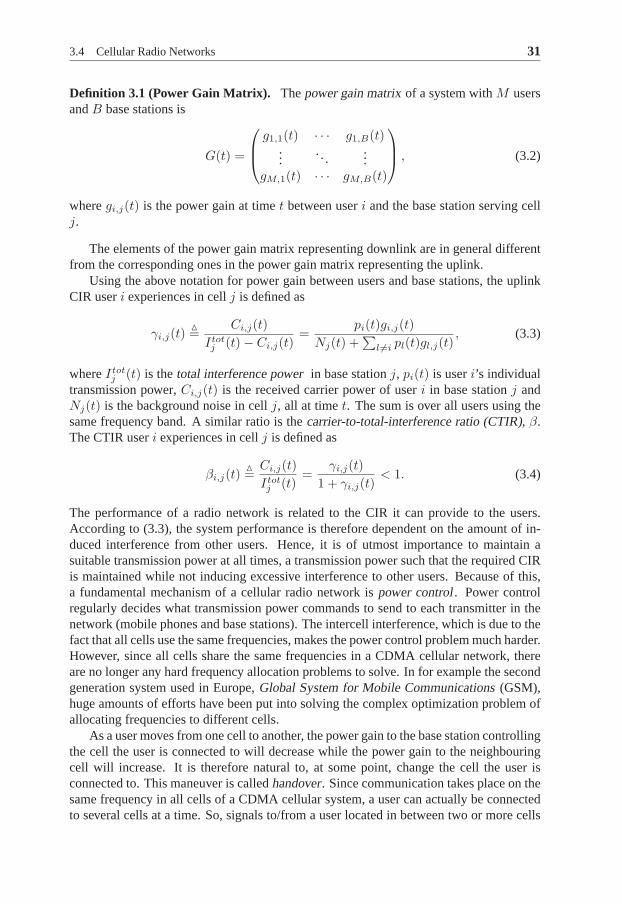
3.4 Cellular Radio Networks 31
Definition 3.1 (Power Gain Matrix). Thepower gain matrixof a system withM usersandB base stations is
G(t) =
g1,1(t) · · · g1,B(t)...
. . ....
gM,1(t) · · · gM,B(t)
, (3.2)
wheregi,j(t) is the power gain at timet between useri and the base station serving cellj.
The elements of the power gain matrix representing downlinkare in general differentfrom the corresponding ones in the power gain matrix representing the uplink.
Using the above notation for power gain between users and base stations, the uplinkCIR useri experiences in cellj is defined as
γi,j(t)△
=Ci,j(t)
Itotj (t) − Ci,j(t)
=pi(t)gi,j(t)
Nj(t) +∑
l 6=i pl(t)gl,j(t), (3.3)
whereItotj (t) is thetotal interference powerin base stationj, pi(t) is useri’s individual
transmission power,Ci,j(t) is the received carrier power of useri in base stationj andNj(t) is the background noise in cellj, all at timet. The sum is over all users using thesame frequency band. A similar ratio is thecarrier-to-total-interference ratio (CTIR), β.The CTIR useri experiences in cellj is defined as
βi,j(t)△
=Ci,j(t)
Itotj (t)
=γi,j(t)
1 + γi,j(t)< 1. (3.4)
The performance of a radio network is related to the CIR it canprovide to the users.According to (3.3), the system performance is therefore dependent on the amount of in-duced interference from other users. Hence, it is of utmost importance to maintain asuitable transmission power at all times, a transmission power such that the required CIRis maintained while not inducing excessive interference toother users. Because of this,a fundamental mechanism of a cellular radio network ispower control. Power controlregularly decides what transmission power commands to sendto each transmitter in thenetwork (mobile phones and base stations). The intercell interference, which is due to thefact that all cells use the same frequencies, makes the powercontrol problem much harder.However, since all cells share the same frequencies in a CDMAcellular network, thereare no longer any hard frequency allocation problems to solve. In for example the secondgeneration system used in Europe,Global System for Mobile Communications(GSM),huge amounts of efforts have been put into solving the complex optimization problem ofallocating frequencies to different cells.
As a user moves from one cell to another, the power gain to the base station controllingthe cell the user is connected to will decrease while the power gain to the neighbouringcell will increase. It is therefore natural to, at some point, change the cell the user isconnected to. This maneuver is calledhandover. Since communication takes place on thesame frequency in all cells of a CDMA cellular system, a user can actually be connectedto several cells at a time. So, signals to/from a user locatedin between two or more cells

32 3 Cellular Radio Communication
can be send/received in several nearby located base stations. A user connected to severalcells is said to be insoft handover. The cells that useri is connected to is called theactiveset, denotedKi. Signals can be received usingmaximum ratio combiningor selectioncombining. Maximum ratio combining utilizes correlation between thereceived signalsmaking the combined CIR equal to the separately received CIRvalues,
γi =∑
k∈Ki
γi,k, (3.5)
Selection combining, on the other hand, means that the combined CIR is simply the max-imum CIR,
γi = maxk∈Ki
γi,k. (3.6)
Since selection combining implies disregarding information, it is less efficient than max-imum ratio combining. The notation introduced so far is summarized in Figure 2.1.
In practice, the users’ signals can not be decoded entirely correct. All users willtherefore experience a degree of self interference, i.e., apart of a user’s own signal willbe experienced as interference. The fraction of the own received signal power that cannot be subtracted in the denominator of (3.3) is called theself interference factor, α. Therelation between a user’s CTIR,β, the user’s perceived CIR,γ, and the self interferencefactor is
γ =C
Itot − (1 − α)C=
β
1 − (1 − α)β. (3.7)
Sinceγ tends to1/α asβ tends to one, a nonzero self interference factor decreases thesystem performance and puts a limit on the maximum CIR that a user can perceive.
Example 3.1: Intercell InterferenceConsider a system with two users and two cells. The power gainmatrix is
G =
(g1,1 g1,2
g2,1 g2,2
)
.
User 1 is solely connected to base station one while user two is initially not connected tothe system at all. User one has a service requiring a carrier-to-interference ratio ofγ1 ifthe self-interference can be neglected. User two’s transmission power is
γ1 =p1g1,1
N⇔ p1 =
γ1N
g1,1,
whereN is the background noise power common to both cells. If user two is providedanother type of service requiring a carrier-to-interference ratio ofγ2 through a connectionwith base station two, the required transmission powers satisfy the following system ofequations
{
γ1 =p1g1,1
N+p2g2,1
γ2 =p2g2,2
N+p1g1,2.
Solving forP = (p1 p2)T yields
P =
(g1,1 −γ1g2,1
−γ2g1,2 g2,2
)−1(γ1
γ2
)
N.

3.5 System Performance 33
Explicitly,
p1 = γ1g2,2 + γ2g2,1
g2,2g1,1 − γ1γ2g1,2g2,1N >
γ1
g1,1N
p2 = γ2g1,1 + γ1g1,2
g1,1g2,2 − γ2γ1g2,1g1,2N.
Thus, user 1’s transmission power is affected by the decision to admit another user, even ifit is in a neighbouring cell. The factor by which user 1’s transmission power is increaseddepends on bothγ1 andγ2.
User 1’s increase in transmission power in the above exampleis to compensate for theincreasedintercell interferencepower.
3.5 System Performance
The performance of the system is quite hard to measure. Firstof all one needs to definewhat we expect from the system. This expectation clearly depends on what kind of useryou are; subscriber or operator.
A subscriber typically expects to have a high probability ofbeing allowed to use thesystem at any given time. This defines a quantity calledGrade of Service(GoS). Onceconnected, the subscriber expects to experience some sort of quality of service(QoS)which is a truly subjective measure. For example, in the caseof a speech service, the sub-scriber expects to hear the other person reasonably well, orin the case of a data-service,that the connection is fast enough without a too long delay. Aconnected subscriber ex-pects to be provided services without being disconnected, something that is consideredfar worse than not getting a connection at all. These different measures, just from thesubscribers point of view, make defining the system performance a hard task.
The operator, who owns and manages the system, also puts expectations on the sys-tem. These can for example be total throughput. However, maximizing the total through-put often comes with a degrade in individual subscriber satisfaction, which then, in thelong run, means less customers for the operator.
This leads to a discussion of which policy to use, i.e., how toprioritize subscribersand what service to give them. The result is of course a trade off between individualsubscriber satisfaction and maximum utilization of the resources.
Different choices of how resources are assigned to users will be compared in thisthesis. For this end, a definition of capacity motivated by Shannon’s theorem on themaximum channel capacity (Wozencraft and Jacobs, 1965, page 520) is made below.
Definition 3.2 (Capacity). Thecapacityis
C△
=∑
i
log2(1 + γi),
where the sum is taken over a set of users.
The set of users considered in the definition depends on whether it is the capacity ofan entire system consisting of several base stations, a single base station or just a single

34 3 Cellular Radio Communication
0 0.1 0.2 0.3 0.4 0.5 0.6 0.7 0.8 0.9 10
1
2
3
4
5
6
7
β = γ1+γ
log2(1
+γ)
α = 0α = 0.1
Figure 3.4: Relation between CTIR,β, and capacity, parameterized by the self in-terference factorα. The capacity loss due to self interfernce is negligible forlowCTIR levels.
user connection. Figure 3.4 shows the relation between a single user’s capacity and CTIRfor two different choices of the self interference factorα. Figure 3.4 implies that the selfinterference factor only has a practical interest for high CTIR values. The self interferencefactor will therefore generally be omitted in the this thesis.
3.6 Radio Resource Management Algorithms
Obviously the ability of a system to provide service is limited. However, it is not as ob-vious in what way it is limited. An always present trade off isthe one between capacity,quality and coverage. It is desirable to provide service to as many subscribers as pos-sible at any given time. Allocating one subscriber a higher data rate or lower bit errorprobability means that his received signal power will be higher and thus higher interfer-ence to other subscribers is introduced. This means that less users can be accommodatedinto the system. Furthermore, since the mobiles’ transmission powers are limited, higherinterference power in the base stations means less coverage.
The choice of which subscribers to admit and what service they will be provided is amatter of policy. The choices which repeatedly have to be made in order to follow thispolicy are done byRadio Resource Management(RRM) algorithms. There is a widerange of RRM algorithms, starting from algorithms making decisions several times eachmillisecond such as fast power control to more long term decisions such as admissioncontrol which considers time periods of whole sessions (e.g., expected length of a phonecall).
3.6.1 Power Control
Power control is used to set the users’ transmission power such that they experience theblock error rate(BLER) they have been guaranteed by other RRM algorithms, while notinducing unnecessary interference power into the system. For uplink capacity reasons
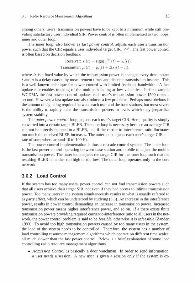
3.6 Radio Resource Management Algorithms 35
among others, users’ transmission powers have to be kept to aminimum while still pro-viding satisfactory user individual SIR. Power control is often implemented as two loops,inner and outer loop.
The inner loop, also known asfast power control, adjusts each user’s transmissionpower such that the CIR equals a user individual target CIR,γtgt. The fast power controlis often based on decision feedback
Receiver:si(t) = sign(γtgti (t) − γi(t))
Transmitter:pi(t) = pi(t) + ∆si(t − n),
where∆ is a fixed value by which the transmission power is changed every time instantt andn is a delay caused by measurement times and discrete transmission instants. Thisis a well known technique for power control with limited feedback bandwidth. A fastupdate rate enables tracking of the multipath fading at low velocities. In for exampleWCDMA the fast power control updates each user’s transmission power 1500 times asecond. However, a fast update rate also induces a few problems. Perhaps most obvious isthe amount of signaling required between each user and the base stations, but most severeis the ability to rapidly raise the transmission powers to levels which may jeopardizesystem stability.
Theouter power controlloop, adjusts each user’s target CIR. Here, quality is simplyconverted into a certain target BLER. The outer loop is necessary because an average CIRcan not be directly mapped to a BLER, i.e., if the carrier-to-interference ratio fluctuatestoo much the received BLER increases. The outer loop adjustseach user’s target CIR at arate of somewhere around 10 to 100 Hz.
The power control implementation is thus a cascade control system. The inner loopis the fast power control operating between base station andmobile to adjust the mobiletransmission power. The outer loop adjusts the target CIR for the inner loop such that theresulting BLER is neither too high or too low. The outer loop operates only in the corenetwork.
3.6.2 Load Control
If the system has too many users, power control can not find transmission powers suchthat all users achieve their target SIR, not even if they had access to infinite transmissionpower. Too many users in the system simultaneously results in what is usually referred toasparty effect, which can be understood by studying (3.3). An increase in the interferencepower, results in power control demanding an increase in transmission power. Increasedtransmission power means higher interference power, and soon. If a there exists finitetransmission powers providing required carrier-to-interference ratio to all users in the net-work, the power control problem is said to befeasible, otherwise it isinfeasible(Zander,1993). To avoid too high transmission powers caused by too many users in the system,the load of the system needs to be controlled. Therefore, thesystem has a number ofload controlling resource management algorithms which operate on different time scales,all much slower than the fast power control. Below is a brief explanation of some loadcontrolling radio resource management algorithms.
• Admission Controlis basically a door watchman. In order to send information,a user needs a session. A new user is given a session only if thesystem is ex-

36 3 Cellular Radio Communication
pected to cope with that user’s request for system resourcesthroughout the entiresession. Note that, being granted a session does not always imply continuous ac-cess to the network resources, see Packet Scheduling and Channel Switching below.Admission control can for example study uplink received power as load measure,see (Choi and Bahk, 2001; Dimitriou et al., 2000; Holma and Laakso, 1999; Huangand Yates, 1996; Ishikawa and Umeda, 1997; Kuri and Mermelstein, 1999; Leiet al., 1999; Outes et al., 2001; Timus and Pettersson, 2001).
• Packet Schedulingis the task of selecting which packet users that will be allowedto send. This is typically done on a time scale of about two to twenty milliseconds.This algorithm only applies to packet users, i.e., not for speech users. Laakso et al.(1998) formulate the packet scheduling problem as an optimization problem. Aspecial mode of WCDMA in which higher data rates can be accomplished at theprice of less fairness is discussed by Kolding et al. (2002).
• Channel Switchinghandles users who already have a session. During the session,a user’s channel conditions and the load of the base stationschange. To adaptto these changes, channel switching increases and decreases the users’ maximumtransmission rate. A lower transmission rate means a lower target SIR. Channelswitching in WCDMA is studied by Gyung-Ho and Dong-Ho (2000).
• Congestion Controlcan be compared to a bouncer at a restaurant. In more extremecases, when neither Channel Switching or Packet Schedulingcan take the systemfrom an overload situation back to the target load, congestion control uses actionswhich are stronger than the previous algorithms. Examples of possible actions are
– denying users’ requests for increased transmission power in the downlink
– move some users to an alternative network, e.g., GSM
– down switching speech users to a worse speech quality or evendrop some realtime users.
Being disconnected is usually consider far more annoying for a user than neverbeing connected at all. Hence disconnection is strongly avoided by the system.
• Link Admission is the algorithm considering users’ requests for augmenting theiractive set with another cell. Important to note here is that the link admission de-cision depends on the downlink only. The reason being that anextra link meanshigher transmission power for the base station serving the new cell. In the uplink,on the other hand, an additional link does not imply increased transmission power.Therefore, the uplink can only gain from more soft handover links.
3.7 WCDMA 37
3.7 WCDMA
The architecture of a WCDMA system contains a number of levels. Starting from celllevel, the service in each cell is provided by a base station,see Figure 3.5. A base stationhosts all lower level (link level) algorithms such as fast power control. The figure also
RNCRNC
BSBS BSBSBS BS
Outside WorldOutside World
Figure 3.5: The architecture of a WCDMA system. The outside world is connectedto the network at Radio Network Controllers (RNC). Each RNC is connected to anumber of base stations (BS). Lower down in the architecture, each base station isconnected to several mobiles.
shows how signals from different base stations are combinedfurther up in the hierarchyin a Radio Network Controller(RNC). A radio network controller receives informationgathered in several cells, even from cells controlled by other RNCs. This, more complete,information about the system as a whole can be used by radio resource managementalgorithms in general and relative load estimates in particular.
A common standard is a requirement for product interaction over manufacture bor-ders. The committee specifying the WCDMA standard is calledThird Generation Part-nership Project(3GPP)2. They specify parameters regarding measurement accuracies,possible data-rate configurations and power control frequency to mention a few. In thissection we will only mention the small part of the standardization process concerning thiswork. To enable reasonable well tracking of the multipath fading while not using too
2http://www.3gpp.org

38 3 Cellular Radio Communication
much bandwidth, the power control feedback has a bandwidth of 1500 bps. The stan-dard states that the system should contain RNCs. Each RNC controls a number of basestations. Since the RNC has knowledge of the situation in a far larger area than a singlebase station does, many of the load controlling schemes reside here such as admission andcongestion control.
An addition to the 3GPP standard is theenhanced uplink(EUL) (3GPP, 2005). Theidea with this addition is to move much of the load controlling algorithms operating on afast time scale from the RNC to the base stations. This decentralization will enable fasterload control. The base stations may also have more accurate information on the currentradio conditions in the base station’s immediate surroundings.
Each base station may control several cells in WCDMA. A user issaid to be insofterhandoverbetween cells in the active set controlled by one base station and in soft han-dover between cells in the active set controlled by different base stations. When usingsofter handover, the signals are combined using maximum ratio combining and whenusing soft handover, selection combining is used. The reason for this is simple, maxi-mum ratio combining requires information about the correlation between the signals asthe combining is done before decoding. Selection combining, on the other hand, is doneafter decoding and therefore only needs a reliability tag such as the estimated receivedCIR for the separately received signals. Hence, soft handover yields selection combiningand softer handover maximum ratio combining. Figure 3.6 explains how the signals arecombined at different levels of the hierarchy.
Central Node
Soft HandoverSelection Combining
Softer Handover Maximum Ratio CombiningMaximum Ratio Combining
Softer Handover
Figure 3.6: The combination of soft and softer handover in a WCDMA system.

4Characterizing Uplink Load
The purpose of this chapter is to characterize uplink load and introduce various waysof looking and approximating it. Inherent properties of CDMA yield that the uplink isinterference limited, i.e., the system performance is limited by the amount of receivedinterference power. A formal definition of uplink relative load is given Section 4.1. Sincean interference limited system is considered, the definition relates load to the amount ofinterference power received in the base stations.
That the uplink is interference limited also means that there is not a one-to-one relationbetween how loaded the system is and, for example, how many channels that are occupied.This makes it harder to determine the fraction of available resources that are currently inuse, compared to systems with a fixed number of channels. Predicting the load is evenharder, since that involves estimating the future receivedinterference power.
Load measures in the literature can be divided into those consideringhard resourcesand those based onsoft resources. These two types of resources will be explained andcompared in Section 4.1.
Another way of dividing the load measures is related to wherethey reside. Resourcemanagement algorithms can reside in a base station. An advantage with this is of coursethat a minimum of signaling is required if the decisions can be made on this intermedi-ate level. Relative load estimates designed to reside in base stations are referred to asdecentralized estimates. Theory related to such estimates is presented in Section 4.2.
A base station has no information about the situation in cells supported by other basestations. Thus, a decentralized estimate can not predict how resource management deci-sions will affect cells supported by other base stations. However, nodes at a higher levelin the system’s architecture have access to information gathered in several cells. Thismore complete information about the system as a whole can be used by load estimates atthis level. Section 4.3 discusses centralized load measures, related to the entire system asopposed to the different base stations.
The theoretical total capacity, thepole capacity, is interesting to study for comparative
39

40 4 Characterizing Uplink Load
purposes, even though it is not achievable in practice. Along the way, pole capacity willbe discussed from the different angles presented here.
Section 4.4 concludes the chapter by discussing different aspects of the presentedapproaches to estimating the uplink load.
4.1 System Load and Capacity
A basic requirement for providing service to users is that there is sufficient power availableto maintain an acceptable QoS. In the uplink this, among other things, means that the totalreceived interference power in the base station must not be too high. The total receiveduplink interference power is
Itot = N +
M∑
i=1
Ci, (4.1)
whereN represents the part of the interference power which is not power controlled byour system. All contributions to the total interference power which originate from ter-restrial non-power controlled sources, such as cellular systems operating at neighbouringfrequencies and electronic equipment in for example cars, are thus embedded intoN .Added to the background noise is the sum of the users’ carrierpowers,Ci for useri. Thesum is taken over allM users in the entire network. In the literature, interference poweris often related to background noise power through theuplink noise rise.
Definition 4.1 (Uplink Noise Rise). Uplink noise rise, Λ, is defined as the total uplinkreceived interference power,Itot, divided by the background noise power,N , i.e.,
Λ△
=Itot
N.
Since the uplink noise rise is the constraining resource, and increasing the number ofactive users or the active users’ quality results in a noise rise increase, there is a naturaltrade off between the number of users and quality. Furthermore, as the users have limitedtransmission power, a higher noise rise means reduced coverage. An always present tradeoff is therefore one between the number of users, quality andcoverage. Perhaps not usefulin practice, but still an educational model is
Quality + Number of users + Coverage = Utilized resources.
The amount of available soft resources is unknown and time varying. An alternative istherefore to estimate theuplink relative loador uplink fractional load, L, i.e., the amountof currently utilized resources relative to the total amount of resources
Quality + Number of users + Coverage =L · total resources.
Since performance of the system is related to the currently received interference power, amore formal definition of load should incorporate this property of the system. One wayis to relate the useful received interference power to the total received interference power.Mathematically this can be expressed as
L =
∑Mi=1 Ci
N +∑M
i=1 Ci
=Itot − N
Itot= 1 − 1
Λ.

4.1 System Load and Capacity 41
Below is a formal definition of load which is inspired what hasbeen said above.
Definition 4.2 (Noise Rise Relative Load).The noise rise relative loadof a CDMAcellular system is defined as
Lnr △
= 1 − 1
Λ. (4.2)
A rearrangement of the expression in the above definition yields thepole equation(Holma and Toskala, 2000)
Λ =Itot
N=
1
1 − Lnr. (4.3)
The equation clearly shows thatLnr = 0 impliesItot = N , i.e., an empty system withonly background noise. As the noise rise relative load approaches one the system isoperated close to the system’s theoretical capacity, thepole capacity, and the interferencepower goes to infinity, see Figure 4.1.
Example 4.1: Noise Rise Relative Load, Single Cell
The total received interference power in a single cell scenario can be expressed as in (4.1).The QoS of each user is related to the carrier-to-total-interference ratio,
βi =Ci
Itot. (4.4)
Solving forCi in (4.4) and inserting it into (4.1) yield
Itot = N +
M∑
i=1
βiItot ⇔ Λ =
Itot
N=
1
1 −∑Mi=1 βi
. (4.5)
The equation has the same form as (4.3) and therefore according to Definition 4.2,
Lnr =
M∑
i=1
βi. (4.6)
The noise rise relative load is clearly a function of the received interference power. Inthe multi cell case, the noise rise relative load is therefore not purely a function of howmany users there are in the system, but also for example wherethe users are located in theradio environment. This means that the pole capacity in terms of e.g., number of users isin general both unknown and time varying. From the inherent requirement of a positivenoise rise and (4.3) we can conclude that a feasible total resource allocation is associatedwith a noise rise relative load between zero and one. Example4.1 shows that the capacityof a CDMA system with conventional receivers (i.e., not utilizing multiuser detection)is in fact interference limitedbecause the interference from other connections limits thecapacity. The opposite is anoise limitedsystem .

42 4 Characterizing Uplink Load
Example 4.2: Noise Limited SystemConsider a system with one user in an isolated cell. The carrier-to-total-interference ratiois
β =C
Itot=
C
N + C< 1,
eliminatingC in this expression gives
Itot =1
1 − βN < ∞.
The total interference power,Itot is finite for all possibleβ sinceβ < 1. In a noise limitedsystem, quality (data rate) is therefore limited by the amount of available transmissionpower.
According to (4.5), the number of users in an interference limited system is, even withunlimited transmission power, limited by the mutual interference power between the con-nections. Furthermore, the amount of additional interference power caused by admittinga new user depends on the current interference power in the system. Figure 4.1 illustratesthe higher interference power contribution of an admitted user at high load, compared tothat at low load. In Figure 4.1,∆Lnr is associated with the amount of noise rise relativeload a user contributes with. For example in a scenario with an isolated cell and perfectpower control,∆Lnr = βtgt for the admitted user according to (4.6). The constantβtgt
is the CTIR that the power control aims at.
0 0.1 0.2 0.3 0.4 0.5 0.6 0.7 0.8 0.9 10
5
10
15
20
Noise Rise Relative Load,Lnr
Noi
seR
ise,Λ
=I
to
t
N[d
B]
∆Lnr
∆Lnr
∆Λ
∆Λ
Figure 4.1: The nonlinear relation between noise rise relative load,Lnr, and noiserise,Λ. ∆Lnr could be the increase caused by admitting another user. Thisgivesdifferent noise rise contribution,∆Λ, at different load levels.
A traditional definition of relative load, which is suitablefor FDMA and TDMA sys-tems, is the number of currently used channels over total number of channels, i.e.,
Ltrad △
=M
Mmax.
A capacity defined as a fixed maximum number of channels is an example of ahard ca-pacity. The hard capacity of a system is fixed and known, unlike thesoft capacity. The
4.2 Decentralized Load 43
soft capacity can only be achieved when a soft resource is studied in the resource man-agement algorithms. Uplink noise rise is an example of asoft resourcesince it dependson time varying variables such as the power gains the users experience. As the uplink ofa CDMA cellular system is limited by this spatial resource, the uplink’s capacity dependson the situation in several cells. If the load is low in surrounding cells, little interferencepower is received from these cells. This results in an increased capacity in the own cellcompared to when the surrounding cells are more loaded. A centralized resource manage-ment algorithm based on a soft resource can, unlike a decentralized algorithm studyinga hard resource, utilize this additional capacity. Example4.4 at the end of the chapterstudies this difference.
In the cases where the soft capacity equals the hard capacity, the traditional definitionof relative load coincides with Definition 4.2. Consider a single cell situation in whichthe only service available is characterized by a target carrier-to-total-interference ratio ofβ0. By using (4.6), the pole capacity can then be calculated as (Lnr = 1 and assumingperfect power control,βi = β0, give the maximum number of users)
1 =Mpole
∑
i=1
β0 = Mpoleβ0 ⇔ Mmax = Mpole =1
β0.
According to (4.6), the noise rise relative load in this scenario is merely the number ofusers timesβtgt. The noise rise relative load can thus be expressed as
Lnr = Mβ0 =M
1/β0=
M
Mmax= Ltrad. (4.7)
Huang and Yates (1996) study a single service scenario with several cells. The totalinterference is therein divided into three parts; background noise,intracell interference,Iown, which is interference from users within the cell, andintercell interference, Iother,which is interference from users in other cells,
Itot = N + Iown + Iother. (4.8)
Since a single service scenario is studied,Iother can be converted into a correspondingnumber of users connected to other base stations,Mother = Iother/C, whereC is thereceived power required to maintainβ0. This once again enables an expression corre-sponding to (4.7), only withM substituted forMown + Mother, whereMown is thenumber of users connected to the own base station.
4.2 Decentralized Load
Some resource management algorithms act in a decentralizednode, in which only localinformation is available. For example, the part of the interference power caused by usersconnected to another base station,Iother, depends on variables not known in the own basestation. Therefore a decentralized estimate has to either measure it or somehow estimateit using local variables only.

44 4 Characterizing Uplink Load
4.2.1 Intercell-to-Intracell-Interference Factor
One way of eliminating the intercell interference from (4.8) is to simply state that it is anominal fraction,f , of the intracell interference, i.e.,
Iother = f Iown.
This is a natural assumption since an increase in interference power in one cell leaks tosurrounding cells. Higher intercell interference power insurrounding cells causes users inthese cells to use higher transmission power, yielding higher intercell interference powerin the own cell. This effect would not be captured ifIother is assumed constant.
Combining the above expression with (4.8) results in an expression forItot that con-tains only local variables
Itot = N + (1 + f)Iown.
According to (4.4), the received power of useri is Ci = βiItot. The interference power
from users in the own cell,Iown, is simply the sum of these user individual carrier powers.An expression for the total interference power is therefore
Itot = N + (1 + f)
Mown
∑
i=1
Ci = N + (1 + f)
Mown
∑
i=1
βiItot.
Solving forItot yields
Itot =N
1 − (1 + f)∑Mown
i=1 βi
.
Once again comparing with (4.3), we see that an approximation of the noise rise relativeload in a multi cell scenario is
Lnr ≈ (1 + f)
Mown
∑
i=1
βi. (4.9)
A comparison with (4.6) shows that one should not consider cells as isolated, since thisgives an underestimation of the noise rise relative load. This is perhaps obvious sinceconsidering cells as isolated corresponds to completely ignoring the intercell interference,Iother in (4.8). Using this technique, the requirement for pole capacity that the noise riserelative load should equal one corresponds to
Mown
∑
i=1
βi =1
1 + f.
Hence, an estimate of the pole capacity is put in terms of combined carrier-to-total-interference ratio. In case of a single service scenario, anestimate of the maximumnumber of users would be
Mmax =
⌊1
(1 + f)β0
⌋
,
where the brackets implies that the ratio should be rounded to the nearest lower integer.The intercell-to-intracell factor,f , is widely used throughout the literature. Boyer et al.

4.3 Centralized Load 45
(2001); Hiltunen and Binucci (2002); Holma and Laakso (1999); Ying et al. (2002); Zhangand Yue (2001) and Sanchez et al. (2002) use it in noise rise relative load expressions. Arange in whichf is usually chosen is between 0.4 and 0.6 if uniformly distributed trafficis expected.
4.2.2 Interference Power Measurements
Another way of considering the entire interference power using only local informationis to simply assume that it is measurable. As concluded in Section 4.1, the increase ininterference power due to an admitted user depends on the interference level. Holma andLaakso (1999) use measurements of the total received interference power,Itot, and ap-proximates the additional interference power a new user would cause through derivativesof (4.3)
∂Itot
∂Lnr=
N
(1 − Lnr)2= Itot 1
1 − Lnr.
An approximative expression for the interference power increase due to an additional loadof ∆Lnr is then
∆Itot =∂Itot
∂Lnr∆Lnr = Itot ∆Lnr
1 − Lnr0
,
whereLnr0 is the noise rise relative load before admitting the new user. An alternative
expression for the interference power increase is derived as the integrated difference inItot,
∆Itot =
Lnr0 +∆Lnr
∫
Lnr0
∂Itot
∂LnrdLnr =
Itot
1 − Lnr0 − ∆Lnr
∆Lnr = Itot(Lnr0 + ∆Lnr) − Itot(Lnr
0 ),
whereItot(Lnr) is the total interference power whenLnr is used in (4.3). The last equal-ity is put there simply as a reminder that integrating a derivate is the same as taking thedifference between the function values at the end points of the integration interval.
Motivated by the calculations leading to (4.6),∆Lnr can be estimated as the newuser’s target CTIR. Using measurements of the total interference power inherently catchesthe variations in intercell interference power. However, it relies heavily on somewhataccurate measurements of the current uplink interference power.
4.3 Centralized Load
The estimates in Section 4.2 can not predict the effects a decision made in one cell willhave on other cells. Users located close to the cell border are especially important. Theseusers can occasionally introduce considerable interference power in other cells as thefollowing example shows.

46 4 Characterizing Uplink Load
Example 4.3: Intercell Interference
Study a prospective user in cellk. Power control will force him to use a transmissionpowerpi satisfying
Ci,k = pigi,k = βtgti Itot
k ⇔ pi = βtgti Itot
k
1
gi,k. (4.10)
Useri’s signal will be received in cellj with a power of
Cij = pigi,j = βtgti Itot
k
gi,j
gi,k.
The received carrier powerCij will in cell j be a part of the intercell interference. Themagnitude ofCij depends on where the user is located. If useri is close to the cell border,gi,j andgi,k will be of the same order andCij will thus to a greater extent contribute tothe noise rise relative load in cellj, compared to the case where useri is close to basestationk.
From a resource management point of view it is quite interesting to have an idea of howmuch load a user will actually induce in the own and surrounding cells. This, however,requires information which is gathered in several cells andan estimate of the noise riserelative load using this information would therefore have to reside in a more centralizedsite than a base station serving just one cell.
4.3.1 Feasibility Relative Load
Thus far, relative load has been related to received interference power. It can equallywell be related to the users’ transmission powers. All work in this section is done underan assumption that a user is power controlled in exactly one cell, i.e., soft handover isnot utilized here. Zander (1993) studies solvability of thepower control equation in thedownlink. The basis for the work is the power control equation, which is derived below.Let useri be power controlled solely from base stationji. Thei:th position of the vectorj thus contains the number of the base station useri is connected to. Useri’s downlinkcarrier-to-interference ratio can be expressed as
γi =Ci
Itoti − Ci
=pigi,ji
Ni +∑
ℓ 6=i plgi,jℓ
=pi
Ni
gi,ji
+∑
ℓ 6=i pℓgi,jℓ
gi,ji
.
Since this is the downlink,pi is the transmission power which information to useri is sentwith. Ni is the background noise useri experiences. Introduce the following matrix andvectors
P (t)△
= [pi(t)], η = [ηi]△
= [Ni
gi,ji
], Z = [ziℓ]△
= [gi,jℓ
gi,ji
] ∈ RM×M .
In a single service system, i.e., allγi = γ0, the above equation for all users can be put inmatrix form
P =γ0
1 + γ0(η + ZP ). (4.11)

4.3 Centralized Load 47
Clearly, it is interesting to study for whichγ0 this equation is solvable (with allpi > 0).Zander (1993) shows that, given knowledge of all power gainsin the system, it is possibleto determine the maximum achievableγ0 in the noise free case,γ∗
0 .For convenience, introduce the notation
λ(A) = max | eig(A)|,for the spectral radius of a matrixA.
Theorem 4.1 (Zander, 1993)Whenever the receiver noise is negligible, there exists, with probability one, a uniquemaximum achievable CIR-level
γ∗0 = sup{γ0|∃P ≥ 0 : γi ≥ γ0∀i}.
The maximum is given by
γ∗0 =
1
λ(Z) − 1,
The power vectorP ∗ achieving this maximum CIR-level is the eigenvector correspondingto λ(Z).
According to Theorem 4.1, simply choosing all users’γtgti less than or equal toγ∗
0
guarantees existence of a positive solution to (4.11) in thesingle service case and inabsence of noise, i.e.,Ni = 0. However, Zander (1993) also states that even in the noisycase, whereNi > 0, the influence of background noise can be made arbitrarily small byscaling all users’ transmission powers with a factor which is large enough.
The above theorem can be used to determine whether or not there is a base stationtransmission power vectorP such that all user achieves the maximum possible C/I-requirement. In a cellular system, it can sometimes be interesting to use a smallerγ0
thanγ∗0 . By formulating and solving a linear programming problem Zander (1993) shows
the following theorem
Theorem 4.2 (Zander, 1993)Wheneverγ0 < γ∗
0 , the power vectorP of least total (sum) power achieving the C/I-levelγ0 will be the solution to the following system of linear equations:
(1 + γ0
γ0E − Z
)
P = N .
whereE denotes the identity matrix.
Thus, by combining Theorem 4.1 and Theorem 4.2, we can conclude that all positiveγ0 < γ∗
0 are possible to achieve. As pointed out by Gunnarsson (2000), requiring allusers’γtgt
i < γ∗0 is a sufficient but not necessary condition in a multi servicescenario.
Thus a load measure based on e.g., the ratio between the maximum currentγtgti andγ∗
0
would be quite conservative. To handle multiple service, introduce the matrixΓtgt whichis a diagonal matrix with the users’ target CIR in the diagonal,
Γtgt △
= diag(γtgt1 , γtgt
2 , . . . , γtgtM ).
Gunnarsson (2000) uses the above ideas to define feasibilityrelative load for multi servicesystems.

48 4 Characterizing Uplink Load
Definition 4.3 (Gunnarsson, 2000). Thedownlink feasibility relative loadis defined as
Lr = inf{µ ∈ R :1
µΓtgt is feasible}.
A set of target CIR:s are said to be feasible if there is a solution to the resultingpower control problem. Gunnarsson (2000) also presents thefollowing theorem to findthe downlink feasibility relative load in a system without soft handover.
Theorem 4.3 (Gunnarsson, 2000)The feasibility relative load,Lr, of a system is
Lr = λ(Γtgt(Z − E)). (4.12)
In case of a feasible system, i.e.,Lr < 1, the transmission powers are
P = (E − Γtgt(Z − E))−1Γtgtη, (4.13)
whereη is aM -dimensional vector with thei:th element equal toNi/gi,i.By using the above theorem it is possible to show that the downlink feasibility relative
load of a single service scenario is the ratio between the target CIR of the only serviceprovided andγ∗
0 in a single service scenario,
Lr = λ(Γtgt(Z − E)) = λ(γ0E(Z − E)) = γ0(λ∗ − 1) =
γ0
γ∗0
. (4.14)
This justifies Definition 4.3, given Theorem 4.1.
4.3.2 Convergence of Power Control Algorithms
Inspired by the presentation done by Hanly and Tse (1999), the uplink interference powerin a multi-cell system is studied. Therein, useri is power controlled solely from one cell,here denoted cellji. Consider a power control algorithm that at each time instant t setsuseri’s transmission power according to
pi(t) = γtgti
Nji
gi,ji
+∑
ℓ 6=i
pℓ(t − 1)gℓ,ji
gi,ji
,
whereNjiis the background noise power useri experiences (which is assumed constant)
and pi(t) is useri’s transmission power at timet. The sum in the above expressionconsiders all users in the entire network. A matrix expression for all users update at timet is therefore
P (t) = Γtgt(N + (ZT − E)P (t − 1)), (4.15)
where
P (t)△
= [pi(t)], N = [Ni]△
= [Nji
gi,ji
], Z = [zℓk]△
= [gℓ,jk
gk,jk
].
The matrixZ will, just as Γtgt, be in RM×M . It is well known from theory of linear
systems (see e.g., Kailath (1980)) that the recursion in (4.15) will converge if and only

4.3 Centralized Load 49
if all eigenvalues ofΓtgt(ZT − E) are within the unit circle. Thus, a measure of theconvergence rate is
Lc = λ(Γtgt(ZT − E)). (4.16)
Note thatZ andZ will have the same eigenvalues if the system is reciprocal, i.e., that thepower gain is equal in uplink and downlink. In this case,
Lc = λ(Γtgt(ZT − E)) = λ(Γtgt(ZT − E)) = Lr.
Example 4.4: Multi Cell Load EstimationStudy a system consisting of three users and two cells in which power control is imple-mented according to (4.15). The power gain matrix is
G =
0.53 0.150.4 0.10.14 0.8
.
Denote the cell represented in the first column I and the second column II. Users1 and2are connected to cell I, see Figure 4.2, and the third user applies for a connection to cellII yielding a j-vector ofj = [1 1 2]. The correspondingZ andZ matrices are thus
Z =
1 1 0.281 1 0.25
0.18 0.18 1
andZ =
1 1.33 0.190.75 1 0.130.26 0.35 1
.
The matrixZ has been given here simply to exemplify the calculation of it, it will not beused in the rest of the example. Note that the upper left two-by-two submatrix ofZ is anall one matrix. This part ofZ corresponds to a single cell system. At first, considerβtgt
i
values according toβtgt
1 = 0.5, βtgt2 = 0.3 andβtgt
3 = 0,
which corresponds to aΓ matrix according to
Γtgt = diag(1 0.43 0
).
This yieldsLc ≈ 0.65 according to (4.16). Figure 4.3a shows how the users’ transmissionpowers converge. After 100 iterations, user three is connected to cell II withβtgt
3 = 0.35.Naturally this affects the transmission powers for all users in the network, as indicatedin Figure 4.3a. Figure 4.3b shows what the different estimates provide in this specificexample. When the new user is admittedLc increases up to approximately0.70. Thus,the fact that admitting a user in one cell requires additional transmission powers for usersconnected to other cells is reflected in an increasedLc. The estimate defined by (4.9)is in the first half, of course, in compliance with the load according to Definition 4.2.However, as the estimate is stationary completely insensitive to the situation in other cells,it eventually settles to the same noise rise relative load asbefore User 3 was admitted.The intercell-to-intracell factor was chosen to zero. In this scenario the true intercell-to-intracell factor when the power control has settled is
f =Iother
Iown=
g3,1p3
g1,1p1 + g2,1p2≈ 0.04.

50 4 Characterizing Uplink Load
1
2
3
?
I II
Figure 4.2: Admission of a new user. User 3 applies for a channel in cell II. Usersconnected to other cells will then experience increased intercell interference power.
As can be seen in the table below,Lr equalsLc. This and other comparisons between dif-ferent load definitions will be discussed in Chapter 6. Table4.1 shows how a decentralizedestimate, such as (4.9), is completely insensitive to what happens in other cells as well asto fluctuations in soft capacity. The example also indicatesthe trade off between cov-
Table 4.1: Four approximations of the uplink load before and after admission ofuser 3.
Users 1,2 Users 1,2,3Lnr = 1 − 1
Λ Eq. (4.2) 0.8 0.84(1 + f)
∑
i βi Eq. (4.9) 0.8 0.8λ(Γtgt(Z − E)) Eq. (4.12) 0.65 0.70λ(Γtgt(ZT − E)) Eq. (4.16) 0.65 0.70
erage and throughput. When a new user is admitted in cellII, the throughput increasesbut the higher transmission power of the users contributes to a decreased coverage due tolimited transmission powers.
4.3.3 Link Based Estimates
An estimate which considers the number of links each user hascan to some extent capturethe soft handover gain. Assuming that maximum ratio combining is used in the combining

4.3 Centralized Load 51
0 20 40 60 80 100 120 140 160 180 2001
2
3
4
5
6
0 20 40 60 80 100 120 140 160 180 2000.6
0.65
0.7
0.75
0.8
Iteration no.
P N
Load
User 1User 2User 3
Eq. (4.2)
Eq. (4.16)Eq. (4.9)
a)
b)
Figure 4.3: Intercell effects. a) Ratio between users’ transmission power and thebackground noise power. b) Noise rise relative load in cell Iaccording to Defini-tion 4.2 and two different estimates of it. A new user is admitted in cell II at iterationnumber 100. The intercell-to-intracell-interference factor, f , is chosen to zero in(4.9).
of the locally received information, a simple way of utilizing the information regardingnumber of links is to assume that each user’s contribution tothe noise rise relative load isinversely proportional to the number of soft handover links. The noise rise relative loadapproximation would then be
Lnrj ≈ (1 + f)
Mj∑
i
βi
ni,
whereMj is the number of users power controlled in cellj andni is useri’s number ofsoft handover links. There has been some studies where link based admission control hasbeen compared with interference power based admission control algorithms. For exampleIshikawa and Umeda (1997) and Gunnarsson et al. (2002) show that using a link basedresource compared to using an interference power based resource in the call admissioncontrol yields approximately the same performance, but thelink based algorithm is farmore sensitive to changes in the radio environment. Since these types of estimates indi-rectly consider variations in the radio environment the users experience, estimated polecapacity will change over time.

52 4 Characterizing Uplink Load
4.4 Discussion
Theory regarding uplink load in cellular CDMA systems is presented in this chapter. Ithas been shown that, despite unlimited transmission power,the capacity of the uplink ofa CDMA cellular radio system is in fact bounded by a finite timevarying capacity, thepole capacity. The uplink is thus interference limited. Since the maximum capacity ofthe system is generally both unknown and time varying a quantity called noise rise rela-tive load was introduced. The noise rise relative load relates the current amount of useduplink capacity to the current maximum uplink capacity, even though both are unknown.Properties of the noise rise relative load has been exploredthrough a survey of differentapproaches to approximating it.
Decentralized Load This type of approximations uses information locally available ineach cell. An advantage with these is of course that they can directly be used in local re-source management algorithms. However, these approximations have no real knowledgeof the effects that resource management decisions have on the surrounding cells. Further-more, a decentralized approximation which makes the assumption that the other cells areequally loaded as the own cell can not fully utilize the soft capacity of a CDMA cellularsystem. In fact, it can be argued that some of these approximations are purely relatedto a hard capacity of the system. Measuring the current totalinterference power is oneway of locally approximate how loaded the surrounding cellsare. This, however, requiresaccurate interference power measurements – something which should not be taken forgranted.
Centralized Load If a centralized approximation is used, information from severalcells can be considered. The type of information may be simply the number of softhandover links each user has or, more advanced, it may be the power gains each userexperiences. Some simplifying assumptions still have to bemade also in the centralizedcases. In the approximation where the number of links is usedfor example, the assump-tion is that the signals received in different base station are combined using maximumratio combining, which is not true in general.
A more theoretical approach has also been handled in the chapter. A definition ofdownlink relative load and feasibility of the downlink power control problem was ex-plored. By using techniques from system theory, solvability of the power control problemhas been associated with a load level below one. As the power control problem is con-cerned with the entire network, this type of load applies to the entire network as opposedto just one base station.

5Approximating Uplink Load
This chapter contains the derivation of a number of uplink load approximations. Sec-tion 5.1 contains a derivation of a set of nonlinear equations for the uplink interferencepower. Different ways of approximately solving the equations lead to two fundamentallydifferent types of approximations. These are derived in Section 5.2. Because of detailsin the current WCDMA standard, information required by the load approximations maynot be available. Approximations explicitly handling thisproblem are also derived. Asmall comparison of the expressions is made in Section 5.3 before Section 5.4 addressesthe sources of estimation errors. Finally, results of a thorough simulation study of theperformance of the approximations is reported on in Section5.7.
It is assumed that the self interference, caused by the base station not being ableto utilize all of the signal received from a user, is assumed negligible in this chapter.Derivation and evaluation of the approximations can also befound in (Geijer Lundinet al., 2003c) and (Geijer Lundin et al., 2003a).
5.1 Uplink Interference Power Expressions
As the name suggests, noise rise relative load is closely related to the uplink noise rise.Therefore, just as the uplink noise rise, the noise rise relative load is a truly spatial quan-tity. A noise rise relative load expression using information gathered in several cells canbe made sensitive to changes in the load caused by changed circumstances in other cells.Below, a number of approximative expressions of the noise rise relative load are derived.These expressions assume power gain values and target carrier-to-total-interference ratiosto be readily available in a central node.
As a starting point for our derivation of the approximations, consider (4.1) only spe-
53

54 5 Approximating Uplink Load
cialized to base stationj,
Itotj = Nj +
M∑
i=1
Ci,j , (5.1)
whereM is the number of users in the entire network andCi,j is the power of the signalfrom useri received in cellj. The signal power from useri in cell j is
Ci,j = pigi,j . (5.2)
wheregi,j is the power gain between useri and base stationj andpi is the transmis-sion power of useri. Combining (5.1) and (5.2) yields an expression ofItot
j in users’transmission powers. Fast power control between base stations and users is employedto counteract the influences of fast changes in the radio environment which is partiallycaused by the multipath fading. Due to a fast update rate and errors in the transmissionpower commands, the momentarily transmission powers are unknown to a central node.However, if the central node is provided with path gain measurement reports it is stillpossible to get an approximative expression of a low pass filtered version the users’ trans-mission powers. The picture is somewhat complicated by the fact that a user’s transmittedsignal is received in several base stations. The information from these base stations canbe combined in three different manners as discussed in Section 3.4. Aside from usingthe correct combination of the signals, it turns out that it will be useful to have approxi-mations of it as well. The following three manners of combining the information will beused in the final noise rise relative load approximations.
Maximum Ratio Combining By approximating the combination of selection combin-ing and maximum ratio combining with just maximum ratio combining, the total com-bined carrier-to-total-interference ratio is approximately the sum of the individually re-ceived carrier-to-total-interference ratios in the separate base stations
βi(t) ≈∑
k∈Ki
gi,k(t)pi(t)
Itotk (t)
, (5.3)
whereKi is the set of cells useri is connected to. The approximation in the above equa-tion is due to a nonlinear relation between CIR and CTIR, see Section 5.4.1. Solving forthe transmission power above yields an approximation of user i’s transmission power attime t,
pi(t) ≈βi(t)
∑
k∈Ki
gi,k(t)Ik(t)
. (5.4)
Inserting this expression into (5.1) yields
Itotj (t) = Nj(t) +
M∑
i=1
pi(t)gi,j(t) ≈ Nj(t) +M∑
i=1
βi(t)gi,j(t)
∑
k∈Ki
gi,k(t)Itot
k(t)
.

5.2 Uplink Load Expressions 55
Selection Combining. The above expression for the interference power in cellj wasderived with an assumption that softer handover is used everywhere. If soft handover isassumed instead, the signals from the different cells are combined using selection com-bining, i.e., the signal with the highest reliability tag ischosen. Consequently, the totalcombined carrier-to-total-interference ratio is
βi(t) = maxk∈Ki
gi,k(t)pi(t)
Itotk (t)
. (5.5)
Maximum Ratio and Selection Combining. Another, more accurate, assumption isto use the correct combination of soft and softer handover. Let useri’s configuration ofsoft and softer handover be defined byKi. The functionc(Ki, G(t), I(t)) corresponds tothe denominator of (5.4) and is a combination of maximum and sums.
Divide the set of base stations useri is connected to, i.e.,Ki, into subsets,Ki,r whereeach subset contains base stations which are all located at one specific physical site. ThesubsetsKi,r are disjunct andKi =
⋃
r Ki,r. The functionc may then by defined as
c(Ki, G, I) ≈ maxr
∑
k∈Ki,r
gi,k
Ik.
Thus, maximum ratio combining is used on the signals received in each separate setKi,r
and selection combining is then applied on the results from the maximum ratio combining.Finally, if the system is maintained at reasonable load levels, it is customary to assumethat the fast power control manages to provideβi ≈ βtgt
i .The three different ways of approximating the transmissionpowers yield three differ-
ent approximative expressions for the uplink interferencepower in cellj.
Itotj (t) ≈ Nj(t) +
M∑
i=1
βtgti (t)
gi,j(t)∑
k∈Ki
gi,k(t)Itot
k(t)
(5.6a)
Itotj (t) ≈ Nj(t) +
M∑
i=1
βtgti (t)
gi,j(t)
maxk∈Ki
gi,k(t)Itot
k(t)
(5.6b)
Itotj (t) ≈ Nj(t) +
M∑
i=1
βtgti (t)
gi,j(t)
c(Ki, G(t), Itot(t))(5.6c)
Applying one of these three equations on all cells in a radio network, i.e., forj =1, 2 . . . B, defines a system of nonlinear equations in the total received interference power.
5.2 Uplink Load Expressions
Three different expressions for the uplink interference power are derived in the previoussection. This section is devoted to solving for the uplink noise rise using these expres-sions. Due to Definition 4.2 of noise rise relative load, there is a one-to-one relation

56 5 Approximating Uplink Load
between uplink noise rise and noise rise relative load. Thus, any of the expressions foruplink noise rise derived here can be converted to an expression for noise rise relativeload.
First are some general methods for solving nonlinear equations given and then twofundamentally different ways of solving the system of nonlinear equations defined by(5.6) will be presented. In order to solve a problem of distributing required information,another set of expressions is given in a separate subsection. Finally, a discussion on howrequired information can be made available is included in this section.
5.2.1 Methods for Solving Nonlinear Equations
Each one of the equations in (5.6) defines a system of nonlinear equations. If an approx-imative solution to these equations can be found, it can be used to approximate the trueload.
There are numerous ways of numerically solving such systemsin the literature. Den-nis Jr. and Schnabel (1983) give some examples. Generally the methods look for a solu-tion to the equationf(x, c) = 0, wherex is a vector of variables andc are parameters ofa general functionf(x, c).
One way of solving the equation is to linearize it or, throughsome other approxima-tion, make the nonlinear equations algebraically solvable. Another way to go is throughnumerical algorithms. The perhaps most famous algorithm istheNewton-Raphson-method,where the approximative solution is, in each step, updated according to
x(i+1) = x(i) −(
df
dx
∣∣∣∣x=x(i)
)−1
f(x(i)).
A problem with this is of course that the derivative off(x) has to be available in algebraicform. If this is not the case, an approximation of the derivative can be used instead. Thisleads to a group of methods commonly referred to asSecant-methods.
If the nonlinear equations can be written on the formx = f(x, c), fix point iterationscan be applied, i.e.,
xi+1 = f(xi, c). (5.7)
Note that convergence of this iteration procedure is not guaranteed in general.Equations (5.6) are on the form given by (5.7), wherex would represent the total
interference power,Itot. In this work, (5.6) have been solved using linear approximationsas well as fix point iterations of the nonlinear equations.
5.2.2 Approximation I: Equal Interference Power In All Cells
For a moment, assume that the interference powers in all cells are the same as in thecell we want to express the interference power in, i.e.,Itot
k = Itotj . Equation (5.6a) then
becomes
Itotj (t) ≈ Nj(t) + Itot
j (t)
M∑
i=1
βtgti (t)
gi,j(t)∑
k∈Kigi,k(t)
. (5.8)

5.2 Uplink Load Expressions 57
The system of coupled nonlinear equations defined by (5.6a) is then simplified into anumber of linear decoupled equations. Solving forItot
j (t) yields an explicit expression ofthe interference power
Itotj (t) =
Nj
1 −∑Mi=1 βtgt
i (t)gi,j(t)P
k∈Kigi,k(t)
. (5.9)
When comparing the above expression with (4.3), it is naturalto associate the uplinkrelative load with
LIMRCj (t)
△
=
M∑
i=1
βtgti (t)
gi,j(t)∑
k∈Kigi,k(t)
, (5.10)
where indexIMRC has been added to indicate that maximum ratio combining has beenused and that the interference powers in all cells were temporarily assumed equal duringthe derivation. This is a practically tractable expressionof the uplink relative load in cellj based on readily available information. The correspondingexpression for uplink noiserise is easily found by dividing (5.9) withNj ,
ΛIMRCj (t)
△
=1
1 −∑Mi=1 βtgt
i (t)gi,j(t)P
k∈Kigi,k(t)
.
Starting from (5.6b) instead yields a different approximative expression forLj(t), namely
LISELj (t)
△
=
M∑
i=1
βtgti (t)
gi,j(t)
maxk∈Kigi,k(t)
, (5.11)
where the indexISEL indicates the assumption of soft handover and equal interferencepower in all cells. The corresponding expression of the uplink noise rise is
ΛISELj (t)
△
=1
1 −∑Mi=1 βtgt
i (t)gi,j(t)
maxk∈Kigi,k(t)
.
Finally the most accurate way of combining the information used in (5.6c) results in yetanother approximative expression for the uplink load
LIBOTHj (t)
△
=M∑
i=1
βtgti (t)
gi,j(t)
b(K,G(t))(5.12)
and for the uplink noise rise
ΛNBOTHj (t)
△
=1
1 −∑Mi=1 βtgt
i (t)gi,j(t)
b(Ki,G(t))
,
whereb(Ki, G) is a function combining elements of theG-matrix according to the con-figuration implied byKi.
To summarize, the following three approximative expressions for the uplink noise risehave been derived.
58 5 Approximating Uplink Load
ΛIMRCj (t)
△
=1
1 −∑Mi=1 βtgt
i (t)gi,j(t)P
k∈Kigi,k(t)
(5.13a)
ΛISELj (t)
△
=1
1 −∑Mi=1 βtgt
i (t)gi,j(t)
maxk∈Kigi,k(t)
(5.13b)
ΛIBOTHj (t)
△
=1
1 −∑Mi=1 βtgt
i (t)gi,j(t)
b(Ki,G(t))
(5.13c)
By using Definition 4.2, the above expressions can be rearranged into expressing the noiserise relative load instead of noise rise. The converted expressions would then equal (4.6)in a single cell system. Note that, when not utilizing soft handover, all expressions in(5.13) will be equal.
5.2.3 Approximation II: Equal Background Noise Power
The other approach to solving the equations defined by (5.6) is to assume equal back-ground noise power in all cells, i.e.,Nj = N . Dividing (5.6a) byN yields
Itotj (t)
N≈ 1 +
M∑
i=1
βtgti (t)
gi,j(t)∑
k∈Ki
gi,k(t)Itotk
(t)
N
.
By using Definition 4.1, the ratio between total received interference power and back-ground noise power can be substituted by the noise rise,Λj ,
Λj(t) ≈ 1 +M∑
i=1
βtgti (t)
gi,j(t)∑
k∈Ki
gi,k(t)Λk(t)
.
This yields a new nonlinear system of equations where the variables are the uplink noiserise in the different base stations. The path gain values arethen known parameters of theequations. This system can be solved through any of the numerical methods previouslydiscussed in Section 5.2.1. Most simple of these is to use theprevious estimate of thenoise rise in base stationk in the right hand side of the above equation
ΛNMRCj (t)
△
= 1 +
M∑
i=1
βtgti (t)
gi,j(t)∑
k∈Ki
gi,k(t)
ΛNMRCk
(t−1)
, (5.14)
whereNMRC indicates that maximum ratio combining and equal background noise inall cells were assumed during the derivation. If the users target CTIR and power gain val-ues are constant or slowly varying, this is a fix point iteration as in (5.7). This expressionof the uplink noise rise can be converted into an expression of the uplink relative loadaccording to
LNMRCj (t)
△
= 1 − 1
ΛNMRCj (t)
. (5.15)

5.2 Uplink Load Expressions 59
Once again, assuming soft handover instead of softer handover provides yet another ex-pression of the uplink noise rise,
ΛNSELj (t)
△
= 1 +
M∑
i=1
βtgti (t)
gi,j(t)∑
k∈Ki
gi,k(t)
ΛNSELk
(t−1)
.
Also in this case, the correct combination of soft and softerhandover can be used
ΛNBOTHj (t)
△
= 1 +M∑
i=1
βtgti (t)
gi,j(t)
c(Ki, g(t),ΛNBOTH(t − 1)),
wherec(K, g,Λ) is a function combining the noise rise vector with theG-matrix accord-ing to the configuration implied by the combination of soft and softer handover (hererepresented byK).
The following three approximations have been derived in this section.
ΛNMRCj (t)
△
= 1 +
M∑
i=1
βtgti (t)
gi,j(t)∑
k∈Ki
gi,k(t)
ΛNMRCk
(t−1)
(5.16a)
ΛNSELj (t)
△
= 1 +
M∑
i=1
βtgti (t)
gi,j(t)
maxk∈Ki
gi,k(t)
ΛNSELk
(t−1)
(5.16b)
ΛNBOTHj (t)
△
= 1 +
M∑
i=1
βtgti (t)
gi,j(t)
c(Ki, g(t),ΛNBOTH(t − 1))(5.16c)
Just as with (5.13), all of these expressions are equal when soft handover is not utilized.The expressions can be rearranged into expressing the noiserise relative load instead.In a single cell system, the corresponding expression for noise rise relative load onceagain coincides with (4.6). In (5.16), one iteration at eachtime update is used. Thiscan be generalized into using several iterations before each update as in Algorithm 5.1.The assumption of slowly varying target CTIR and power gain values can then be relaxed.Denote byβtgt a vector containing the users’ target carrier-to-total-interference ratios andby the integerN iter the number of fix point iterations performed before each update. By
Algorithm 5.1Let Λ(t, 0) = Λ(t − 1)Assign one of the right hand sides of (5.16) tof(Λ, βtgt, G)Forn = 1 to N iter
For j = 1 to BLet Λj(t, n) = f(Λ(t, n − 1), βtgt, G)
Λ(t) = Λ(t,N iter)
using fix point iterations like these, the expressions catchfrequent updates in path gainmeasurements better. Convergence of this algorithm when using (5.16a) is analyzed inChapter 6.

60 5 Approximating Uplink Load
5.2.4 Approximation III: Distributed Information
A complication concerning the distribution of required information is that the base sta-tions may deliver the path gain measurement reports to different central nodes. For ex-ample according to the 3GPP standard, a user initiating its session in an area covered bya central, call itRNC2, and during the session moves to an area supported by anotherRNC, RNC1, will not report path gain measurements toRNC1 but toRNC2. A userlocated insideRNC1’s service area may thus introduce considerable interference powerto the base stations without delivering any path gain reports toRNC1. All the above ex-pressions for uplink noise rise can only consider users reporting path gain measurementsto the central the estimate resides in. Besides the obvious solution to neglect users notreporting their path gain, a set of noise rise approximations which are a combination ofthe techniques used in the two previous sections is proposed. Below is a derivation ofthe alternative expression which approximates the noise rise in base stations belonging toRNC1.
Split the sum over users in the (5.6) into two sums, one being over the users reportingtheir path gain measurements toRNC1 and the other over users reporting to other centralnodes (here represented byRNC2). Exemplifying with (5.6a)
Itotj (t) = Nj +
∑
i∈RNC1
βtgti (t)
gi,j(t)∑
k∈Ki
gi,k(t)Itot
k(t)
+∑
i∈RNC2
βtgti (t)
gi,j(t)∑
k∈Ki
gi,k(t)Itot
k(t)
. (5.17)
Here cellj belongs toRNC1. Consider just the sum over users inRNC2 and approx-imateItot
k (t) in (5.17) with the total received interference power in basestationj. Thisallows us to approximate the sum as
∑
i∈RNC2
βtgti (t)
gi,j(t)∑
k∈Ki
gi,k(t)Itot
k(t)
≈ Itotj (t)
∑
i∈RNC2
βtgti (t)
gi,j(t)∑
k∈Kigi,k(t)
.
Substituting the second sum in (5.17) by the above expression and solve forItotj (t) yield
Itotj (t) =
Nj +∑
i∈RNC1βtgt
i (t)gi,j(t)P
k∈Ki
gi,k(t)
Itotk
(t)
1 −∑i∈RNC2βtgt
i (t)gi,j(t)P
k∈Kigi,k(t)
.
Assume thatNj = Nk = N and thatΛk(t) = Λk(t− 1). Dividing the above equation byN then results in an expression of the uplink noise rise which is a combination of (5.13a)and (5.16a)
ΛRNCMRCj (t)
△
=
1 +∑
i∈RNC1βtgt
i (t)gi,j(t)P
k∈Ki
gi,k(t)
ΛRNCMRCk
(t−1)
1 −∑i∈RNC2βtgt
i (t)gi,j(t)P
k∈Kigi,k(t)
.

5.2 Uplink Load Expressions 61
Note that the sum in the denominator represents the noise rise relative load that usersreporting toRNC2 introduce to cellj. Neglecting these users results in a larger denomi-nator, which yields a smaller approximation.
This approximation is interesting sinceRNC2 can now send a message toRNC1
containing the additional noise rise relative load that users belonging toRNC2 intro-duce in each cell controlled byRNC1. This message would then be far smaller than onecontaining the complete path gain information regarding these users. Obviously soft han-dover can be assumed to be used everywhere here as well, or theactual combination ofsoft and softer handover can be assumed. This gives three types of expressions using thetechnique with sending relative load information between different RNCs.
ΛRNCMRCj (t)
△
=
1 +∑
i∈RNC1βtgt
i (t)gi,j(t)P
k∈Ki
gi,k(t)
ΛRNCMRCk
(t−1)
1 −∑i∈RNC2βtgt
i (t)gi,j(t)P
k∈Kigi,k(t)
(5.18a)
ΛRNCSELj (t)
△
=
1 +∑
i∈RNC1βtgt
i (t)gi,j(t)
maxk∈Ki
gi,k(t)
ΛRNCSELk
(t−1)
1 −∑i∈RNC2βtgt
i (t)gi,j(t)
maxk∈Kigi,k(t)
(5.18b)
ΛRNCBOTHj (t)
△
=1 +
∑
i∈RNC1βtgt
i (t)gi,j(t)
c(Ki,G(t),ΛRNCBOT H(t−1)
1 −∑i∈RNC2βtgt
i (t)gi,j(t)
b(Ki,gi,k(t))
(5.18c)
5.2.5 Required Information
All the above derived expressions for the uplink load rely onknowledge of users’ tar-get carrier-to-total-interference-ratio,βtgt, which are assumed known by the system.They also need path gain measurements, which can be made available in two differentways: (3GPP, 2000a, 1999)
M1: The mobile stations are requested to periodically(but not necessarily synchronously) report pilotpower measurements. As an example, pilot powerfrom the six strongest base stations can be reportedat a rate of 0.5 Hz.
M2: For handover purposes, the mobile typically re-ports similar measurements in an event-drivenfashion. It measures the pilot powers from theneighboring cells and reports up to the six strongestpath gains at handover events.
In both cases, the channel is assumed reciprocal, i.e., the uplink path gain is assumedapproximately equal to the corresponding downlink path gain with respect to distancedependent path loss and shadow fading. Multi path fading is assumed filtered out in the

62 5 Approximating Uplink Load
lower layer filtering. Furthermore, these different strategies only provide data from a lim-ited set of mobile-to-base path gains. The remaining path gains, however, are consideredsmall and set equal to zero. According to the 3GPP standard the individual measure-ment errors in relative path gain should not be greater than 1.5 dB with a probability of90% (3GPP, 2000a).
5.3 Comparison of the Uplink Load Expressions
In the previous section two fundamentally different ways ofsolving the nonlinear systemof equations implied by (5.6a) are presented. The approximate expressions derived inSection 5.2.2 which assume the interference power to be equal in all cells, may at firstseem redundant since other expressions which are derived under far more reasonable as-sumptions are available, the ones assuming equal background noise. The approximationsΛIMRC , ΛISEL andΛIBOTH have, however, one major advantage compared to the iter-ations. When trying to approximate the uplink noise rise in base stationj, the interferencepower in base stationk was approximated with that in base stationj, i.e.,Itot
k = Itotj . In
the case base stationj is the base station with the highest interference power in the area,this implies, starting with (5.6a),
Itotj ≈ Nj +
M∑
i=1
βtgti
gi,j∑
k∈Ki
gi,k
Itotk
≤ Nj +
M∑
i=1
βtgti
gi,j∑
k∈Ki
gi,k
Itotj
= Nj + Itotj
M∑
i=1
βtgti
gi,j∑
k∈Kigi,k
= LIMRCj .
This property of the estimate can be useful when using the estimate in RRM algorithms.Since the approximation is likely to be higher then the true load, the RRM algorithms willreceive an earlier warning of a potential future congestion.
The main strength of the above expressions for uplink load isthat they, like the trueinterference power, depend on the actual situation in several cells and do not rely on anintercell-to-intracell-interference factor,f . Furthermore, since the expressions involvethe users’ carrier-to-total-interference target, users who require high transmission powerwill inherently be given less coverage if an expression likethis is used in the resourcemanagement algorithms. To exemplify, study (5.10)
LIMRCj (t) =
M∑
i=1
βtgti (t)
gi,j(t)∑
k∈Kigi,k(t)
.
Each users’ contribution is a product of the target carrier-to-total-interference ratio and aratio between path gains. A user far from the own base stationbut close to another, willhave a small gain to its own base station (gi,k) and a relatively large gain to the otherbase station (gi,j). Therefore, the ratio of the path gains will be relatively large which canbe compensated for with a small target carrier-to-total-interference ratio. This one of theideas used for designing radio resource allocation algorithms in Chapter 7.

5.4 Sources of Estimation Errors 63
5.4 Sources of Estimation Errors
A number of different effects and approximations degrade the performance of the loadapproximations. These include:
• The nonlinear relation between CIR and CTIR (see Section 5.4.1)
• TX increase (see Section 5.4.2)
• The soft(er) handover assumption
• Imperfect power control
• The assumption regarding relation between the uplink interference power, alterna-tively the background noise power, in different base stations
• The assumption that unknown path gains are equal to zero
• Path gain measurement errors according to 3GPP (2000a) and sparsely sampledpath gain measurement reports
These error sources’ affect on the approximation accuracy is investigated through simu-lations in Section 5.7.
5.4.1 Nonlinear Relation Between CIR and CTIR
When deriving (5.3) it is assumed that the sum over the received CTIR in different basestationsk, βi,k, equals theβi which is required by the user’s service, i.e.,
βi =∑
k∈Ki
βi,k.
This is not true in general where there may be more than one term in the sum, even if∑
k∈Kiγi,k = γi. A simple proof is
∑
k∈Ki
βi,k =3∑
k=1
γi,k
1 + γi,k≥
3∑
k=1
γi,k
1 + γi=
γi
1 + γi= βi,
where equality holds if and only if two of theγi,k:s are zero (which corresponds to no softhandover). Thus, the sum over the separately received CTIR is larger than the experiencedCTIR. Therefore, this contributes to under estimating the users’ transmission powers.
How big the difference is depends on the relation between theseparately received CIRvalues; if a user is almost solely connected to one base station, the difference is small. Thecombined CIR also influences how big the difference is. The bigger the combined CIR is,the bigger the difference may be.
64 5 Approximating Uplink Load
5.4.2 TX Increase
For simplicity, assume that all users in the system is power controlled form exactly onebase station. TX increase is a result of fast power control adjusting each user’s transmis-sion power to compensate for multi path fading dips in the power gain between mobile andconnected base station. The mobile uses a high power during deep fades. This may yielda considerable interference increase to neighboring cellssince a dip in the power gain tothe connected base station does not always imply an, as deep,dip to the neighboring basestations.
To exemplify, consider a scenario where mobile one is connected to base station two.We are interested in its interference power contribution tobase station three. Due topower control, each user’s transmission power is approximately inversely proportional tothe momentary power gain between the user and the controlling base station, i.e.,
p1 ∝ 1
g1,2.
Base station three will receive the signalp1g1,3 which is proportional to the ratio betweenthe momentarily power gains, i.e.,
C1,3 ∝ g1,3
g1,2.
The path gain reports provided by the users do not include multi path fading (the actualreported value is low pass filtered;F{gi,j}). Since the uplink load approximations, unlikefast power control, use users’ path gain reports there will be a part of the uplink interfer-ence power that will not be counted for in the approximations. Essentially, it is possible toobserveF{g1,3}
F{g1,2}but notg1,3
g1,2, which is related to the actual interference power contribution
in base station three. In Figure 5.1a, the ratio of low-pass filtered versions of the path gainmeasurements (solid) is plotted. Of course this will not detect the high peaks in the ratioof the momentarily power gains (dashed). Perhaps momentarily sharp peaks are tolerableby base station three. A better model could therefore be to consider the low-pass filteredload contribution which is essentially proportional to a low pass filtered version of the ra-tio between the power gain to base station three and base station one,F{ g1,3
g1,2}. However,
as indicated by Figure 5.1b, the load contribution is still underestimated. Essentially, thisexemplifies Jensen’s inequality (Billingsley, 1995)
f(E(x)) ≤ E(f(x)),
wheref(x) is a convex function andE(x) denotes the expected mean with respect tox.The solid line in the Figure 5.1b thus represents the quantity used in our expressions of theaverage noise rise while the dashed line represents the quantity that corresponds to useri’s actual contribution to the average uplink noise rise in base stationj. This additionalcontribution in inter-cell-interference is referred to asTX increase, defined as follows.
Definition 5.1 (TX increase). TheTX increase, τ , of a connection is the ratio betweenexpected transmission power with multipath fading and the expected transmission powerwithout multipath fading.

5.5 TX Increase Compensation 65
0.03 0.04 0.05 0.06 0.07 0.08 0.09 0.10
2
4
6
8
0.03 0.04 0.05 0.06 0.07 0.08 0.09 0.10.5
1
1.5
2
2.5
time [s]
time [s]
a)
b)
Figure 5.1: a) Ratio between filtered power gain measurementsF{gi,j}F{gi,k}
(solid) and
momentary measurementsg1,3
g1,2(dashed). The momentary high peaks in the ratio
between the momentary measurements are not present in the ratio between the fil-tered versions. b) Ratio between filtered measurements (solid) and filtered ratio,F{ g1,3
g1,2} (dashed). The average of the filtered ratio between momentary measure-
ments (dashed) is higher than the ratio between the filtered measurements (solid).
Since the uplink load expressions, unlike fast power control, use power gain reportsfrom users, the approximations do not include the part of theuplink load caused by TX in-crease.
Aside from the approximations, there are ideas of how to schedule transmission insuch a way that transmission during deep fades are avoided. This will make the varianceof the momentary power gain values less and hence decrease the TX increase effect. Anexample of such a work is Törnqvist et al. (2004). TX increasehas been studied by e.g.,Ariyavisitakul and Chang (1993); Hashem and Sousa (1999) and Sipilä et al. (1999).
5.5 TX Increase Compensation
Boujemaa et al. (2002); Sipilä et al. (1999) provide expressions for the average trans-
66 5 Approximating Uplink Load
mission power increase when utilizing the diversity gain ofa rake receiver. Sipilä et al.(1999) also concludes that the expressions, which are derived under an assumption ofperfect power control, are reasonable even with imperfect power control. The amount ofadditional average intercell interference power induced by TX increase is a function ofhow many multi path fading rays the receiver considers and the relative strength thesehave. A first result is that in case there areN equally strong rays the interference poweris increased a factorN/(N − 1). We study a more general and practically interestingcase, where the rays have different strength. If the strength of each received multi pathray, Xk, k = 1, 2 . . . , N can be assumed exponentially distributed, the weighted sum,∑
akXk, will have a probability density function which can be approximated by
N∑
k=1
πk
ake− x
ak , x ≥ 0
whereπk is
πk =
N∏
i=1,i 6=k
ak
ak − ai. (5.19)
This is an approximative expression because perfect utilization of each received multipath ray was assumed during the derivation. Let the coefficients ak be normalized sothat their sum equals 1. The expected average transmission power increase can now beexpressed as
τ =
N∑
k=1
aN−2k log(ak)
∏Ni=1,i 6=k ak − ai
,
N∑
k=1
ak = 1, (5.20)
whereτ is the ratio between expected transmission power with multipath fading andthe transmission power without. Note, that the above expression requires all the relativestrengths,ak, to be unique. In a practical scenario, however, this is always the case.
Given the characteristics of the radio channel, and assuming that these characteristicsare the same in all surrounding cells, it is thus possible to calculate a factorτi,j whichapproximates the additional received carrier power from user i in base stationj. The fac-tors can then be used by the noise rise approximations in (5.13) and (5.16). Accordingly,Algorithm 5.1 can be adjusted to incorporate this TX increase compensation. This ideais used in Algorithm 5.2 which is applicable to a system not using soft handover. Thealgorithm is only exemplified withΛNMRC , of course any other of the recursions derivedearlier can be applied. This assumes allak to be unique. The corresponding algorithm
Algorithm 5.2
Let Λiter,TX(t, 0) = Λiter,TX(t − 1)Forn = 1 to Niter
For each base stationjLet Λiter,TX
j (t, n) = 1 +∑M
ℓ=1 βtgtℓ (t)
gℓ,j(t)Pk∈Kℓ
gℓ,k(t)
Λiter,T Xk
(t,n−1)
τℓ,j(t)
Λiter,TX(t) = Λiter,TX(t,Niter)
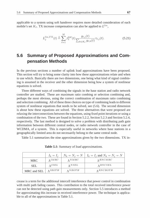
5.6 Summary of Proposed Approximations and Compensation Methods 67
applicable to a system using soft handover requires more detailed consideration of eachmobile’s setKℓ. TX increase compensation can also be applied toLlin,
Llin,TXj (t)
△
=
M∑
ℓ=1
βtgtℓ (t)
gℓ,j(t)∑
k∈Kℓgℓ,k(t)
τℓ,j(t). (5.21)
5.6 Summary of Proposed Approximations and Com-pensation Methods
In the previous sections a number of uplink load approximations have been proposed.This section will try to bring some clarity into how these approximations relate and whento use which. Basically there are two dimensions, one being what kind of signal combin-ing is assumed in the receiver and the other dimension being how a system of nonlinearequations is solved.
Three different ways of combining the signals in the base station and radio networkcontroller are studied. These are maximum ratio combing or selection combining and,perhaps the most obvious, using the correct combination of maximum ratio combiningand selection combining. All of these three choices on type of combining leads to differentsystem of nonlinear equations that needs to be solved, see (5.6). The second dimensionis about how these equations are solved. The three alternatives that were proposed arerelaxing the interconnections between the equations, using fixed point iterations or using acombination of the two. These are found in Section 5.2.2, Section 5.2.3 and Section 5.2.4,respectively. The last method is designed to solve a problemwith distributing path gaininformation between different central nodes, or radio network controller in the case ofWCDMA, of a system. This is especially useful in networks where base stations in ageographically limited area do not necessarily belong to the same central node.
Table 5.1 summarizes the nine approximations given by the two dimensions. TX in-
Table 5.1: Summary of load approximations.
Ik = Ij Nk = Nj = N Ik = Ij andNk = Nj = N
MRC ΛIMRC ΛNMRC ΛRNCMRC
SEL ΛISEL ΛNSEL ΛRNCSEL
MRC and SEL ΛIBOTH ΛNBOTH ΛRNCBOTH
crease is a term for the additional intercell interference that power control in combinationwith multi path fading causes. This contribution to the total received interference powercan not be detected using path gain measurements only. Section 5.5 introduces a methodfor approximating this increase in received interference power. The technique is applica-ble to all of the approximations in Table 5.1.

68 5 Approximating Uplink Load
5.7 Simulations
Performance of the load approximations derived in this chapter is in this section evaluatedusing simulations. The simulator models many of the characteristics of a true system. SeeAppendix A.1 for more details of the simulator. The performance of the approximationsin terms of mean and standard deviation of single errors willbe evaluated for differentload levels. Reasons for the approximation errors will alsobe discussed along the way.
5.7.1 Simulation Setup
The simulator used when evaluating the performance of the approximations is discussedin Appendix A.1. The simulation area is a system of 21 base stations located at 7 differentsites. In order to avoid border effects in the outermost cells, a wrapping technique hasbeen used. The wrapping applies to both interference and user movement.
For the purpose of evaluating the performance of the expressions for noise rise derivedin Section 5.2, momentary true uplink noise rise and all the approximative expressions forit is sampled every frame, i.e., 100 times a second. The true noise rise is calculated usingDefinition 4.1, in which the interference power is found using (4.1).
Measurements of path gains are subject to errors according to (3GPP, 2000a), i.e. a90% confidence interval of 1.5 dB. The users’ inability to report path gain to all basestations is modeled through limiting each report to the six strongest base stations. This isalso the maximum number of cells that is reported in a WCDMA system.
The total power gain is calculated using two factors;gs and gmp. Antenna gain,distance attenuation and shadow fading are all representedby gs while gmp represents thevariations caused by the multi path fading. The true noise rise is thus calculated accordingto
Λj(t) =N +
∑Mi gs
i,j(t)gmpi,j (t)pi(t)
N,
whereN is a constant representing the thermal noise only.Each approximative expression in Section 5.2 is then compared to the true noise rise,
time instant by time instant. In the following sections of this chapter, statistics of theresulting differences in noise rise are reported for different true noise rise levels.
Two different bit rates are used in the simulations, 64 kbps and 192 kbps. The usershave no upper transmission power limit in order to isolate the sources of estimation errorsconsidered here.
5.7.2 Measurement Report Frequency
The approximative expressions in Section 5.2 rely on measurements of the path gainsbetween user and base station. In reality, complete knowledge of the entire path gainmatrix is not available since path gain reports are sparselyspread in time and they donot cover all base stations. Therefore this section is devoted to studying the expressions’sensitivity to limited path gain knowledge. As a comparison, Figure 5.2 shows averageerror ofΛNBOTH andΛIBOTH (which both can be found in (5.16)) when knowing thewhole uplink path gain matrix and actual receivedβi. Already under these relativelyidealistic circumstances, an effect of approximating the interference power in all cells
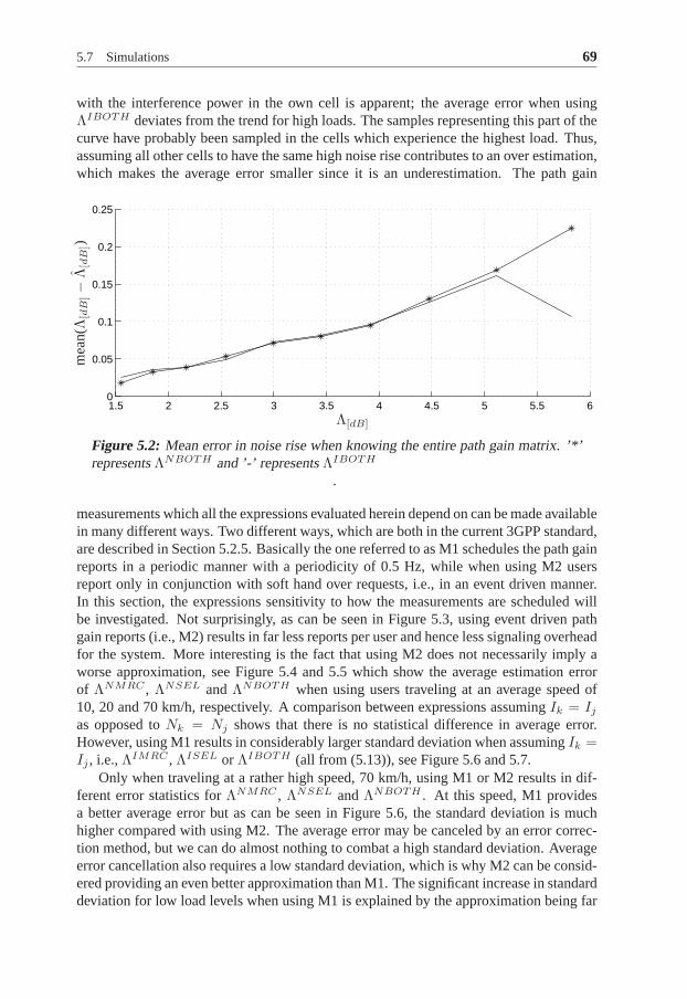
5.7 Simulations 69
with the interference power in the own cell is apparent; the average error when usingΛIBOTH deviates from the trend for high loads. The samples representing this part of thecurve have probably been sampled in the cells which experience the highest load. Thus,assuming all other cells to have the same high noise rise contributes to an over estimation,which makes the average error smaller since it is an underestimation. The path gain
1.5 2 2.5 3 3.5 4 4.5 5 5.5 60
0.05
0.1
0.15
0.2
0.25
Λ[dB]
mea
n(Λ[d
B]−
Λ[d
B])
Figure 5.2: Mean error in noise rise when knowing the entire path gain matrix. ’*’representsΛNBOTH and ’-’ representsΛIBOTH
.
measurements which all the expressions evaluated herein depend on can be made availablein many different ways. Two different ways, which are both inthe current 3GPP standard,are described in Section 5.2.5. Basically the one referred to as M1 schedules the path gainreports in a periodic manner with a periodicity of 0.5 Hz, while when using M2 usersreport only in conjunction with soft hand over requests, i.e., in an event driven manner.In this section, the expressions sensitivity to how the measurements are scheduled willbe investigated. Not surprisingly, as can be seen in Figure 5.3, using event driven pathgain reports (i.e., M2) results in far less reports per user and hence less signaling overheadfor the system. More interesting is the fact that using M2 does not necessarily imply aworse approximation, see Figure 5.4 and 5.5 which show the average estimation errorof ΛNMRC , ΛNSEL andΛNBOTH when using users traveling at an average speed of10, 20 and 70 km/h, respectively. A comparison between expressions assumingIk = Ij
as opposed toNk = Nj shows that there is no statistical difference in average error.However, using M1 results in considerably larger standard deviation when assumingIk =Ij , i.e.,ΛIMRC , ΛISEL or ΛIBOTH (all from (5.13)), see Figure 5.6 and 5.7.
Only when traveling at a rather high speed, 70 km/h, using M1 or M2 results in dif-ferent error statistics forΛNMRC , ΛNSEL andΛNBOTH . At this speed, M1 providesa better average error but as can be seen in Figure 5.6, the standard deviation is muchhigher compared with using M2. The average error may be canceled by an error correc-tion method, but we can do almost nothing to combat a high standard deviation. Averageerror cancellation also requires a low standard deviation,which is why M2 can be consid-ered providing an even better approximation than M1. The significant increase in standarddeviation for low load levels when using M1 is explained by the approximation being far

70 5 Approximating Uplink Load
from accurate in a few instants. The statistics is thus somewhat misleading in this case.It is the users that are close to the cell border that are the most important ones to have
somewhat accurate path gain knowledge of since these are theusers that cause most ofthe inter-cell-interference. Since these users are more likely to change their soft handoversetup compared to users within the cell, using M2 thus mean that it is also more likely thatthese users provide reports. Simulations shown in this section implies that scheduling theusers’ path gain reports in a event driven manner, such as M2,provides an at least equallygood approximation of the uplink noise rise while requiringless signaling overhead.
100
101
102
103
104
10−1
100
101
102
103
Frame no
No.
ofre
port
spe
rus
er
Figure 5.3: Cumulative sum over number of reports per user for M1 (solid)and M2(dashed)
1.5 2 2.5 3 3.5 4 4.5 5 5.5 60
0.5
1
1.5
2
Λ[dB]
mea
n(Λ[d
B]−
Λ[d
B])
ΛNMRC
ΛNSEL
ΛNBOTH
Figure 5.4: Mean error in noise rise. User speed: 10 km/h. Solid:M1, dashed:M2.
5.7.3 One Radio Network Controller
In the previous section it is shown that the expressions are practically independent ofthe type of path gain reporting, periodic or event-based, and therefore only event-basedreports are considered in this section.

5.7 Simulations 71
1.5 2 2.5 3 3.5 4 4.5 5 5.5 6 6.5 7−0.5
0
0.5
1
1.5
2
2.5
Λ[dB]
mea
n(Λ[d
B]−
Λ[d
B])
ΛNMRC
ΛNSEL
ΛNBOTH
Figure 5.5: Mean error in noise rise. User speed: 70 km/h. Solid:M1, dashed:M2.
1.5 2 2.5 3 3.5 4 4.5 5 5.5 6 6.5 70
0.1
0.2
0.3
0.4
0.5
Λ[dB]
std(
Λ[d
B]−
Λ[d
B])
ΛNMRC
ΛNSEL
ΛNBOTH
Figure 5.6: Standard deviation of single noise rise errors. All is for 70km/h.solid:M1, dashed:M2
1.5 2 2.5 3 3.5 4 4.5 5 5.5 6 6.5 70
0.5
1
1.5
Λ[dB]
std(
Λ[d
B]−
Λ[d
B])
ΛIMRC
ΛISEL
ΛIBOTH
Figure 5.7: Standard deviation of single noise rise errors.All is for 70km/h.solid:M1, dashed:M2

72 5 Approximating Uplink Load
Uniform Traffic With Single Service
Figure 5.8 shows the performance of four different expressions when using 64 kbpsstreaming users. As each user has no more than one link, assuming soft or softer han-dover makes no difference in this scenario. The major gap between the lines is due toTX increase (see Section 5.4.2), since multi path fading is not simulated in the runs cor-responding to the dashed lines. The conclusion from this figure is that TX increase doesgive a considerable contribution to the total error. Also, all four expressions produce anunderestimate of the uplink noise rise, mainly due to that measurements of all path gainsare not available. A part of the error due to TX increase can beeliminated by using the
1 2 3 4 5 6 70
0.2
0.4
0.6
0.8
1
1.2
1.4
1.6
1.8
2
Λ[dB]
mea
n(Λ[d
B]−
Λ[d
B])
Figure 5.8: Error in noise rise with 64 kbps users. One link per user. Dashed: Nomulti path fading. ’o’:ΛIMRC , ’x’: ΛNMRC , ’+’: ΛISEL, ’*’: ΛNSEL. TX increaseclearly has an impact on the approximations.
expressions for the additional transmission power in Section 5.5. If the factors by whichthe separate received multi path rays are weighted with, i.e., ak in (5.19), are known itis possible to apply Algorithm 5.2. Figure 5.9 shows that it is then possible to eliminatemost of the error in average. In Figure 5.10 a more realistic scenario is shown whereeach user is allowed up to three handover links at a time. First of all, assuming softerhandover (ΛIMRC andΛNMRC) gives larger average error compared to assuming softhandover (i.e.,ΛISEL andΛNSEL) or both soft and softer handover (i.e.,ΛIBOTH andΛNBOTH ). This is natural since assuming softer handover everywhere means overesti-mating the system’s ability to correctly receive signals, which in turn means underesti-mating the required transmission powers. Under these circumstances, i.e., almost equalload in all cells, the errors from all six expressions are small in average and has fairlylow standard deviation. Using any of the approximations in (5.16) provides equal averageerror as those in (5.13), but with lower standard deviation.This is explained by the factthat assuming equal background noise power makes the performance of the expression
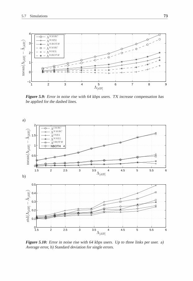
5.7 Simulations 73
1 2 3 4 5 6 7 8 9−1
0
1
2
3
4
Λ[dB]
mea
n(Λ
[dB
]−
Λ[d
B])
ΛNMRC
ΛNSEL
ΛNBOTH
ΛNMRC
ΛNSEL
ΛNBOTH
Figure 5.9: Error in noise rise with 64 kbps users. TX increase compensation hasbe applied for the dashed lines.
1.5 2 2.5 3 3.5 4 4.5 5 5.5 6
0
0.5
1
1.5
2
NBOTH 4
1.5 2 2.5 3 3.5 4 4.5 5 5.5 60
0.1
0.2
0.3
0.4
0.5
Λ[dB]
Λ[dB]
mea
n(Λ
[dB
]−
Λ[d
B])
std(Λ
[dB
]−
Λ[d
B])
ΛNMRC
ΛNSEL
ΛIMRC
ΛISEL
ΛIBOTH
a)
b)
Figure 5.10: Error in noise rise with 64 kbps users. Up to three links per user. a)Average error, b) Standard deviation for single errors.

74 5 Approximating Uplink Load
independent of different load in different cells. The approximationsΛNMRC , ΛNSEL
andΛNBOTH all use the previous approximation to approximate each user’s contributionto the noise rise. By looking at (5.16a), which is repeated below, it is apparent that un-derestimating the noise rise at timet− 1 results in underestimating every term in the sumthat constitutes the noise rise at timet
ΛNMRCj (t) = 1 +
M∑
i=1
βtgti
gi,j∑
k∈Ki
gi,k
ΛNMRCk
(t−1)
.
As can be expected, the performance ofΛNBOTH andΛIBOTH can be described as anaverage of the two other assumptions regarding soft or softer handover. The two middlelines in the Figure 5.10a representΛIBOTH andΛNBOTH . The figure shows that theyapproximate the noise rise with an average error less than 0.5 dB while maintaining alow standard deviation even for high true noise rise levels,see Figure 5.10b. The slightincrease in error as the noise rise increases, may be explained by looking in the load do-main. As mentioned in the introduction, even a small difference in load gives a substantialincrease in noise rise at high load levels. This also means that a small load error resultsin a large noise rise error when operating at high load levels. In Figure 5.11 statistics forload expressions are plotted versus true load computed according to (4.2),
L = 1 − 1
Λ,
whereΛ is given by the simulator. There is no dramatic increase in error as the loadof the system increases in this domain. All the lines in the figure are quite straight butdo not have the correct incline. This can best be explained bystudying (5.10). Ideally,the expression is a sum over all users in the network. The factthat for example the linerepresentingLIMRC in Figure 5.11 does not have the correct incline is thus an effect ofeach user’s contribution being underestimated and that notall users are considered dueto limited path gain reports. All the expressions have a sum over, ideally, all the users,shown in (5.16a), and hence the same reasoning applies. To summarize, there are tworeasons why the lines in Figure 5.10 deviates from a straightline for high load levels:
• even a minor error at high loads produces a non-negligible error in the noise rise
• the sum representing the load approximation has a larger error due to many users,all with a minor underestimated contribution.
Hot Spot
When derivingΛIMRC , ΛISEL andΛIBOTH in Section 5.2.2 the interference power wasassumed to be approximately equal in all cells. This is an assumption that is unsuitable forscenarios with hot spots, i.e., when one or several base stations have considerably higherload than the others. As can be seen in Figure 5.12a) all expressions still provide a prettygood average noise rise approximation for moderate noise rise levels. However, underthese circumstancesΛISEL is useless due to its errors have a high standard deviation atheavily loaded cells. In order to explain the severe over estimation done byΛISEL at high

5.7 Simulations 75
0 0.1 0.2 0.3 0.4 0.5 0.6 0.7 0.8 0.9 10
0.2
0.4
0.6
0.8
1
L
L
Figure 5.11: Error in uplink load when using 64 kbps users.LIMRC : ’o’,LNMRC ’x’, LISEL: ’+’, LNSEL: ’*’. The curve L = L is also shown.
loads, study a scenario where user1 is connected, by soft handover, to base stationsj andℓ. Since both base stations are in the active set, the path gains from the user to the basestations, i.e.,g1,j andg1,ℓ, cannot differ too much. IfItot
j is much greater thanItotℓ , than
the contribution from user1 is according to (5.6b)
g1,jβtgt
1
max{ g1,j
Itotj
,g1,ℓ
Itotℓ
} = g1,jβtgt
1
g1,ℓItotℓ (5.22)
while it is reflected inΛISEL by
g1,jβtgt
11
Itotj
max{g1,j , g1,ℓ}= g1,j
βtgt1
max{g1,j , g1,ℓ}Itotj . (5.23)
If Itotj ≫ Itot
ℓ , the load contribution (5.22) is likely highly overestimated using (5.23).This explainsΛISEL’s overestimation of the load in highly loaded cells, as illustrated inFigure 5.12. The high standard deviation is a result of the expressions alternating betweenbeing an over estimation in the case of different interference levels in neighboring basestations and under estimation in the case of almost equal interference levels.ΛNBOTH
provides approximations with both low average error and lowstandard deviation.
5.7.4 Several Radio Network Controllers
The knowledge on users’ path gains can be even further limited by considering reportsfrom only a subset of the users. As argued in Section 5.2.4, some users will not report theirpath gain to the RNC they are currently controlled by if they started their session whenlocated in an area served by another RNC. In this section we have used path gain reportsaccording to the scheduling technique referred to as M2 and compared the performanceof the expressions defined by (5.18) for different fractionsof external users (i.e., usersnot reporting their path gain to the RNC referred to asRNC1 in Section 5.2.4). As a

76 5 Approximating Uplink Load
1 2 3 4 5 6 7−1
0
1
2
3
NBOTH 4
1 2 3 4 5 6 70
1
2
3
4
Λ[dB]
Λ[dB]
mea
n(Λ
[dB
]−
Λ[d
B])
std(Λ
[dB
]−
Λ[d
B])
ΛNMRC
ΛNSEL
ΛIMRC
ΛISEL
ΛIBOTH
a)
b)
Figure 5.12: Error in noise rise with 64 kbps users. Three links. Hot spot.a)Average approximation error. b) Standard deviation of single approximation errors.

5.8 Summary 77
comparison, statistics for the expression that completelyignores the external users arealso studied. Figure 5.13-5.15 show the average estimationerror when 10, 20 and 30%of the users report to another RNC than the one they are closest to, respectively. Clearly,just ignoring that some users are not considered in the expression can be quite drastic.However, when using an expression that incorporates an estimate of the load contributionfrom the external users (i.e.,ΛRNCMRC , ΛRNCSEL or ΛRNCBOTH ), the performanceis almost equal to the case where measurement reports from all users are available. Acomparison between Figure 5.10b and Figure 5.16 shows that the expressions studied inthis section have approximately the same standard deviation as the ones assuming equalbackground noise power in all cells.
The expressions in (5.13) are not shown here. The problem of not receiving path gainreports from some users can be solved in the same way, i.e., with small messages betweendifferent RNCs, without any additional changes to the expressions.
1.5 2 2.5 3 3.5 4 4.5 5 5.5 60
0.5
1
1.5
2
2.5
3
3.5
Λ[dB]
mea
n(Λ[d
B]−
Λ[d
B])
MRCSELBOTH
Figure 5.13: Mean errors in noise rise when using two RNCs. Solid: All reports,dashed: Reports in one RNC, dashdotted:ΛRNC . 10 % of the users report to anotherRNC.
5.8 Summary
This chapter focused on establishing the noise rise relative load in a practical system.Combining expressions for the total received interferencepower in different base stations,resulted in a system of nonlinear equations. Two conceptually different methods for ap-proximately solving this system were proposed. The choice of method for solving thesystem of equations together with different methods for combining information receivedin different base stations gave a large number of different approximations. By using in-formation gathered in several cells, they all explicitly consider the intercell interferencepower. This means that they are in fact sensitive to the system’s soft capacity. Since thechannels’ path gain values are considered by the approximations, the approximations arecompletely robust to any changes in the radio environment, such as different propagationexponents.

78 5 Approximating Uplink Load
1.5 2 2.5 3 3.5 4 4.5 5 5.5 60
1
2
3
4
Λ[dB]
mea
n(Λ[d
B]−
Λ[d
B])
MRCSELBOTH
Figure 5.14: Mean errors in noise rise when using two RNCs. Solid: All reports,dashed: Reports in one RNC, dashdotted:ΛRNC . 20 % of the users report to anotherRNC.
1.5 2 2.5 3 3.5 4 4.5 5 5.5 60
1
2
3
4
Λ[dB]
mea
n(Λ[d
B]−
Λ[d
B])
MRCSELBOTH
Figure 5.15: Mean errors. Solid:All reports, dashed:Reports in one RNC,dashdot-ted:ΛRNC . 30 % of the users report to another RNC.
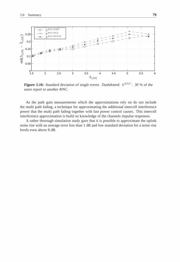
5.8 Summary 79
1.5 2 2.5 3 3.5 4 4.5 5 5.5 60
0.05
0.1
0.15
0.2
0.25
Λ[dB]
std(
Λ[d
B]−
Λ[d
B])
ΛRNCMRC
ΛRNCSEL
ΛRNCBOTH
Figure 5.16: Standard deviation of single errors. Dashdotted:ΛRNC . 30 % of theusers report to another RNC.
As the path gain measurements which the approximations relyon do not includethe multi path fading, a technique for approximating the additional intercell interferencepower that the multi path fading together with fast power control causes. This intercellinterference approximation is build on knowledge of the channels impulse responses.
A rather thorough simulation study gave that it is possible to approximate the uplinknoise rise with an average error less than 1 dB and low standard deviation for a noise riselevels even above 8 dB.

80 5 Approximating Uplink Load

6Analyzing Uplink Load
This chapter studies uplink load from a theoretical perspective. Alternative definitionsof uplink load related to the entire system as opposed to justone cell are introduced.Definitions explicitly relating uplink load to existence ofa solution to the power controlproblem of finding appropriate transmission powers for all users are also introduced. Amatrix conveniently representing the interconnections between different base stations isintroduced. The matrix is then used as a basis for deriving much of the results in thischapter as well as in the following ones. In this chapter the matrix is used to providelinks between the uplink load approximations in Chapter 5 and the rather theoretical def-initions of uplink load introduced in this chapter. Towardsthe end, much of the resultsare condensed into a method for approximating the uplink load in practice. Section 6.2introduces alternative definitions of uplink load and discusses how the load of a systemaccording to these definitions can be determined. In Section6.4 relations between differ-ent definitions of uplink relative load as well as some of the expressions in the previouschapter are established. All expressions for the uplink load in the previous chapter are de-rived through approximations of a system of nonlinear equations. Some of the expressionsuse iterations. Sufficient conditions for convergence of one of the iterations are developedin Section 6.5. Divergence of the iterations will also be related to a lower bound of theuplink load.
Since this is a theoretical study, it is assumed that the system has complete knowledgeof all power gains. Furthermore, the users’ experienced CTIR will be assumed to equalthe target CTIR set by the resource management algorithms. This corresponds to studyingthe steady state of a perfect power control algorithm.
81
82 6 Analyzing Uplink Load
6.1 System Properties
In this section, a number of properties of a system will be stated in order to simplify thepresentation of quantities and results given in the remaining part of the chapter.
6.1.1 Terminology
The connections between users and base stations can be conveniently gathered in a matrix.
Definition 6.1 (Link Matrix). The element on rowℓ and columnj of the link matrix,K ∈ R
M×B , is defined as
Kℓ,j△
=
{
1, if userℓ is power controlled by base stationj
0, otherwise.
The setsKℓ can thus be depicted as
Kℓ = {j : Kℓ,j = 1}.
Correspondingly,cj , the set of users power controlled by base stationj, can be defined as
cj△
= {ℓ : Kℓ,j = 1}.
Let N ∈ RB×1 be a vector with the base station individual background noise powers. A
system with link matrixK and power gain matrix defined according to Definition 3.1 inwhich the background noise powers in the different cells aregiven by the vectorN andthe users have target carrier-to-total interference ratios according to the diagonal matrixBtgt is denoted(Btgt, G,K,N).
Definition 6.2 (System Feasibility). A system(Btgt, G,K,N) is feasibleif there existmobile individual finite positive transmission powers suchthat
βℓ ≥ βtgtℓ ∀ℓ.
Otherwise, the system isinfeasible.
Adopt a terminology stating that a user with links to a numberof base stations is saidto beconnectedto those base stations. To quantify the number of base stations mobiles ina network are connected to and power controlled by, strict connectivity and connectivityare introduced.
Definition 6.3 (Strict Connectivity). A system is said to havestrict connectivityk if atleast one mobile is connected tok base stations.
Definition 6.4 (Connectivity). A system is said to haveconnectivityk if at least onemobile is power controlled byk base stations.
To exemplify the last two definitions, consider a system withjust one user who isin soft handover between two cells, but the power gain to one of the base stations ismuch higher than that to the other one. The user is thus connected to both base stations

6.1 System Properties 83
but power controlled by just one of them. The system then has strict connectivity two butconnectivity one. On the other hand, when in softer handover, the user is power controlledby both base stations and the connectivity is then also two.
As concluded in Example 4.3, the interference power a user causes in base stationj is proportional to the ratio betweengi,j andgi,Ki
in a system with connectivity one.In connection with the example, these ratios were gathered in a matrix. Here, a similarmatrix, therelative power gain matrix, is defined.
Definition 6.5 (Relative Power Gain Matrix). The element on rowi and columnj oftherelative power gain matrix, Z ∈ R
M×B , is at timet
zi,j(t)△
=gi,j(t)
∑
k∈Kigi,k(t)
.
6.1.2 Interference Power Expression
A system with connectivity one is more simple to analyze theoretically. All mobiles essen-tially communicate with one base station in a system with connectivity one. For example,it is possible to establish a matrix expression for the received interference powers.
Combining (5.1) and (5.2) yields (suppressing the time index, t)
Itotj = Nj +
M∑
i=1
pigi,j .
If useri is solely connected to base stationKi,
βi =Ci,Ki
ItotKi
= pigi,Ki
ItotKi
,
where the first equality is the definition ofβi (see (3.4)). Solving forpi and inserting itinto the above expression forItot
j yield
Itotj = Nj +
M∑
i=1
βigi,j
gi,Ki
ItotKi
= Nj +
M∑
i=1
βizi,jItotKi
.
The above sum over users can be split into two sums,
Itotj = Nj +
B∑
k=1
∑
i∈ck
βizi,jItotKi
= Nj +B∑
k=1
∑
i∈ck
βizi,jItotk . (6.1)
The core of the framework developed here is the system matrix.
Definition 6.6 (System Matrix). The element on rowk and columnj of the systemmatrix, L ∈ R
B×B , isLk,j(t)
△
=∑
i∈ck
βtgti (t)zi,j(t).

84 6 Analyzing Uplink Load
Given the link matricesK, relative power gain matrixZ and the users’ target CTIRvalues in a diagonal matrixBtgt,
L = KT BtgtZ. (6.2)
With the purpose of expressing the total interference powers in (6.1) in vector form, as-sume perfect power control. This justifies substitutingβi by βtgt
i which makes it possibleto write (6.1) as
Itotj =
B∑
k=1
Lk,jItotk .
The vector expression corresponding to (6.1) is then
Itot = LT Itot + N ⇔ Itot = (E − LT )−1N. (6.3)
6.2 System Load
6.2.1 System Noise Rise Relative Load
Even though a relative load per cell is interesting from a practical point of view since itis used with advantage in the resource management, a load related to the entire system isequally interesting from a theoretical point of view. One ofthe conclusions in Chapter 4 isthat the uplink noise rise is a natural load measure in the uplink. Therefore, the followingdefinition of system load is a natural one to make.
Definition 6.7 (System Noise Rise Relative Load).Thesystem noise rise relative loadis defined as
Ls△
= maxj
Lnrj ,
whereLnrj is the uplink noise rise relative load in cellj according to Definition 4.2.
The expressions for uplink noise rise relative load in Chapter 5 can thus be used toapproximate the system noise rise relative load, e.g.,
LIMRCs
△
= maxj
LIMRCj
LISELs
△
= maxj
LISELj .
6.2.2 Feasibility Relative Load
Yet another definition of load is one based on the system as a whole, i.e., not as consistingof a number of small systems (cells). The load of a system can then be explicitly relatedto existence of a solution to the system’s power control problem of finding appropriatetransmission powers to satisfy all users’ requirements on carrier-to-interference ratios.
The distance to infeasibility according to Defintion 6.2 wasexpressed by Herdtner andChong (2000) as afeasibility margin. Later, feasibility margin was related tofeasibilityrelative loadby Gunnarsson (2000). In these references the quantities were expressed interms of CIR. Below, these quantities are redefined in terms of CTIR instead.

6.2 System Load 85
Definition 6.8 (Feasibility Margin). The feasibility margin, Γm, of a cellular system,(Btgt, G,K,N), is defined as
Γm△
= sup{x ∈ R :(xBtgt, G,K,N
)is feasible}.
Clearly,Γm > 1 corresponds to a feasible system. The interpretation ofΓm is that itis the largest factor by which all users’ target CTIR values can be scaled without losingfeasibility. The relation to the, within automatic controlwell known quantity, gain marginis obvious.
The alternative load measure can now be defined in terms of thefeasibility margin.
Definition 6.9 (Feasibility Relative Load). Thefeasibility relative load, Lf , of a system(Btgt, G,K,N) is defined as
Lf△
=1
Γm= inf{µ ∈ R :
(1
µBtgt, G,K,N
)
is feasible}.
System feasibility is a necessary condition for stability of distributed power con-trol (Gunnarsson, 2000; Herdtner and Chong, 2000; Yates, 1995; Zander, 1993). Notethat system infeasibility together with unlimited uplink transmission powers imply an in-finite received interference power in some cell. This, in turn, implies that the uplink noiserise relative load equals one in at least one cell. Conversely, the system is feasible if thesystem noise rise relative load in Definition 6.7 is less thanone.
The following theorem is used here merely to give some intuition for Definition 6.8and Definition 6.9. The result is the same and the proof similar to those given by Zander(1993), only this is applicable to the uplink as opposed to the original theorem which isderived for the downlink.
Theorem 6.1A noise-less single-service system with connectivity one,(β0E,G,K,0B), has a maxi-mum achievable carrier-to-total-interference ratio of
β∗0 = max{β0|Itot
j > 0∀j ∈ [1, B], βi ≥ β0∀i ∈ [1, M ]}.Furthermore, the maximum is given by
β∗0 =
1
λ(ZT K),
whereZ is the system’s relative power gain matrix.
Proof: According to 6.2, the system matrix in a single service scenario is
L = β0KT EZ,
whereβ0 is the target CTIR of the only service provided andE is the identity matrix inR
M×M . Applying (6.3) to a noise-less scenario yields
ZT KItot =1
β∗0
Itot = λItot.
The smallest realλ which gives a positive real solutionItot is the greatest eigenvalue ofKZT , λ(ZT K), according to theory for positive matrices, see Appendix A.2. Since alargerβ∗
0 corresponds to smaller eigenvalues ofKZT , 1β∗
0= λ(ZT K).

86 6 Analyzing Uplink Load
The same result applies also for a system with noise as Theorem 6.2 will show. Giventhe above result that a maximumβ0 does exist, the intuitive choice of feasibility marginand feasibility relative load in a single service system,
Γm =β∗
0
β0andLf =
β0
β∗0
,
are true if the system has connectivity one.The definition of feasibility relative load above is similarto Definition 4.3. They
are, however, not equal since Definition 6.9 uses target carrier-to-total-interference (βtgt)ratios instead of target carrier-to-interference ratios (γtgt) but most of all, Definition 4.3is concerned with the downlink. Note thatLf has the desirable properties thatLf ≥ 0and that a system is feasible if and only ifLf < 1.
6.3 Estabilishing the Feasibility Relative Load
This section is devoted to finding an expression for the feasibility load. Connectivity oneand higher connectivity will be handled in separate subsections.
6.3.1 Connectivity One
The system propertyLf can be found in systems with connectivity one by using Theo-rem 6.2 below. For convenience introduce
λ(L)△
= max eig (L),
for the maximum eigenvalue of the matrixL.
Theorem 6.2 (Feasibility Relative Load)In a system(Btgt, G,K,N) with connectivity one, the feasibility uplink relative load is
Lf = λ(L).
Proof: According to Definition 6.9, the feasibility relative load is the infimumµ such that( 1
µB,G,K,N) is feasible. The system is feasible if there are finite positive transmission
powers such thatβtgti ≤ βi. Sinceβi > 0 andgi,Ki
> 0,
pi =βi
gi,Ki
ItotKi
> 0 ⇒ IKi> 0.
The feasibility relative load is thus the smallest realµ yielding a positive solutionItot ≻ 0to
Itot � 1
µLT Itot + N. (6.4)
Let us first consider a noise-free scenario, i.e.,N = 0,
Itot � 1
µLT Itot ⇔ LT Itot � µItot,

6.3 Estabilishing the Feasibility Relative Load 87
where the inequalities should be interpreted element wise.According to Perron-Frobeniustheory for positive matrices, the smallest realµ such that there is anItot = Itot
0 > 0that satisfies the inequality is the maximum eigenvalue toLT , see Appendix A.2. Now,consider a scenario with target CTIR values1µ+ǫβ
tgti , ǫ > 0. The inequality is then
strictly satisfied,
Itot0 ≻ 1
µ + ǫLT Itot
0 ⇔ Itot0 =
1
ǫ + µItot0 + ∆,
where∆ ≻ 0. Therefore, it is always possible to choose ak > 0 such that
k∆ � N.
To conclude, the smallestµ + ǫ such that there is a positive solutionItot to (6.4) isλ(LT ).
The feasibility relative load is obviously related to the users’ target CTIR and theintercell interference they cause, even though often not assimple as in the case with thenoise rise relative load. Example 6.1 studies a simple single service scenario with just twocells.
Example 6.1: Feasibility Relative Load, Single ServiceConsider a system consisting of two cells in which the only service provided requires atarget CTIR ofβ0. If soft handover is not utilized, the system matrix is
L =
(M1β0 β0
∑
i∈c1zi,2
β0
∑
i∈c2zi,1 M2β0
)
,
whereM1 andM2 are the number of users connected to base station one and two,respec-tively. Assume an average relative power gain per cell of0.4, i.e.,
1
M1
∑
i∈c1
zi,2 =1
M2
∑
i∈c2
zi,1 = 0.4.
According to Theorem 6.2, the feasibility relative load is the maximum eigenvalue of thesystem matrix. Given a target maximum feasibility relativeload,Lmax
f , an upper boundonM2 is
M2 ≤Lmax
f − M1β0
β0(Lmaxf − (1 − 0.42)M1β0)
Lmaxf .
This gives the relation between the system capacity and the capacity of cell one accordingto Figure 6.1 whenβ0 equals0.1 or 0.3. Choosing a smallerβ0 yields smaller maximaltotal capacity. On the other hand, a smallerβ0 enables admitting more users. This resultconcurs with the statement that higher throughput comes with less fairness, i.e., by givingmore resources to a few users the throughput is increased, but more users will experiencepoor or no service at least momentarily.
Another observation is that the maximum capacity is reachedwhen the resources areshared between the base stations. This is a result of less interference when fewer usersare connected to the same base station.

88 6 Analyzing Uplink Load
0 0.2 0.4 0.6 0.8 1 1.2 1.4
1.3
1.4
1.5
1.6
1.7
1.8
1.9
2β0 = 0.1β0 = 0.3
M1 log2(1 + γ0)
(M1
+M
2)lo
g2(1
+γ0)
Figure 6.1: Maximum combined capacity in cell one and two, as a function of thecapacity in cell one in Example 6.1.Lmax
f = 0.8.
Example 6.2: Feasibility Relative Load, Multi Service
Consider a system with two users and two base stations in which user one is controlledby base station one and user two by base station two. The link matrix and the power gainmatrix are
K =
(1 00 1
)
andG =
(0.8 0.32g2,1 0.7
)
,
respectively. According to Theorem 6.2, the feasibility relative load is the maximumeigenvalue ofBtgtZ.
The upper bound onβtgt2 is therefore
βtgt2 ≤ βtgt
1 − Lf
βtgt1 (1 − z1,2z2,1) − Lf
Lf .
Figure 6.2 shows the relation betweenβtgt1 andβtgt
2 such that the feasibility relativeload is 0.8 for two different values ofg2,1. The figure shows that we can allow a highervalues forβtgt
2 for a givenβtgt1 wheng2,1 is smaller. Ag2,1 = 0 would give a straight
horizontal line atβtgt2 = Lf .
Remark6.1. Since soft handover can only decrease the uplink load, aLf found usingTheorem 6.2 in a system with connectivity one will be an upperbound of the load in thecorresponding system with soft handover.
An application of Theorem 6.2 is to show thatLf equals the natural definition offeasibility relative load in a single service scenario
Lf = λ(KT BtgtZ) = λ(βtgt0 KT Z) = βtgt
0 λ(KT Z) = β0λ∗ =
βtgt0
β∗0
.

6.3 Estabilishing the Feasibility Relative Load 89
0 0.1 0.2 0.3 0.4 0.5 0.6 0.7 0.80
0.2
0.4
0.6
0.8
βtgt1
βtg
t2
g2,1 = 0.5g2,1 = 0.2
Figure 6.2: Relation betweenβtgt1 andβtgt
2 such thatLf = 0.8 in Example 6.2.
6.3.2 Higher Connectivity
A special case of connectivity higher than one is that all users are power controlled by allbase stations. Hanly (1996) shows that, in this special case, the system is feasible if
M∑
i=1
βtgti ≤ B.
Using Defintion 6.9 of feasibility relative load yields
Lf =
∑Mi=1 βtgt
i
B.
In the general case of higher connectivity, where the users are power controlled by arbi-trarily many base stations, a matrix expression can no longer be obtained for the receivedinterference powers. There are also numerous combinationsof methods for combiningsignals received in different base stations. If all signalsare combined using maximumratio combining the received interference powers are the solution to (5.6a), i.e.,
Itotj = Nj +
M∑
i=1
βtgti
gi,j∑
k∈Ki
gi,k
Itotk
, j = 1, 2, . . . , B.
Introduce the functions
fj(Btgt, G,K,N, I)
△
= Nj(t) +
M∑
i=1
βtgti (t)
gi,j(t)∑
k∈Ki
gi,k(t)Itot
k(t)
, j = 1, 2, . . . , B.
The idea is to approximate these functions with linear functions about a point,Itot0 ∈ R
B ,and then use the theory for positive matrices that was previously used in the proof ofTheorem 6.2. LetL(Itot
0 ) be the jacobian matrix off . Each elementLℓ,j(Itot0 ) of L(Itot
0 )is defined by
Lℓ,j(Itot0 )
△
=∂fj(B
tgt, G,K,N, Itot)
∂Itotℓ
=∑
i∈cℓ
βtgti
gi,j
(∑
k∈Ki
gi,k
Itotk
)2
gi,ℓ
Itotℓ
2 , j, ℓ = 1, 2, . . . , B.

90 6 Analyzing Uplink Load
Based on this linear approximation, the feasibility relative load with arbitrarily connec-tivity can be approximated as
Lf ≈ λ(L(Itot
0 )).
6.4 Relative Load Comparisons
In a single cell system the relative load according to Definition 4.2, Definition 6.7 andDefinition 6.9 are the same according to the following theorem.
6.4.1 Connectivity One
Theorem 6.3In a single cell system with multiple services, the relativeload according to Definition 4.2,Definition 6.7 and Definition 6.9 equals
Lf =
M∑
i=1
βtgti = Lnr = Ls.
Proof: It is shown in Example 4.1 that the uplink noise rise relativeload in a single cellsystem is the sum of the users’ target CTIR. Since it is a single cell system, this musttrivially be the system noise rise relative load as well.
When it comes to the feasibility relative load, first note thatall relative power gainsare one in a single cell system. The system matrix is then simply the sum of users’ targetCTIR,
L =M∑
i=1
βtgti .
Thus, the feasibility relative load equals the noise rise relative load in single cell system.
In a multi cell system, the feasibility relative load is smaller than the noise rise relativeload.
Theorem 6.4In a feasible noise-flat system with connectivity one,
Lf ≤ Ls.
Proof: Let us first make the following transformation
Lf ≤ Ls ⇔ 1
1 − Lf≤ 1
1 − Ls= max
jΛj .
Therefore, it is sufficient to prove that11−Lf≤ maxj Λj . Similar to the maximum eigen-
value, introduceλ(A)
△
= min | eig A|,

6.4 Relative Load Comparisons 91
for the eigenvalue ofA with the smallest magnitude. In a noise-flat system the maximumnoise rise is
maxj
Λj = maxj
(E − LT )−11 = ||(E − LT )−1||∞ ≥ λ((E − LT )−1),
where the second equality is true since the system is feasible, see Appendix A.2. Theabove inequality is true since, according to Skogestad and Postlethwaite (1996),
λ(A) ≤ ||A||.
It remains to prove thatλ((E − LT )−1) equals1/(1 − Lf ),
λ((E − LT )−1) =1
λ((E − LT ))=
1
1 − λ(LT )=
1
1 − Lf.
Other results, which are perhaps more useful in practice, are the following two theo-rems. Introduce
Llocalj
△
=∑
ℓ∈cj
βtgtℓ ,
for the load users connected to cellj cause in the own cell.
Theorem 6.5 (Bound on Feasibility Relative Load)Consider a noise-flat system with connectivity one. The feasibility relative load,Lf , isbounded below and above by
maxj
Llocalj ≤ Lf ≤ max
jLIMRC
j .
Proof: See Appendix A.4.
Corollary 6.1 (Sufficient Condition for Stability)A noise-flat system with connectivity one is feasible if
maxj
LIMRCj < 1.
Proof: Follows from Theorem 6.5 and the fact that a system is feasible if Lf < 1.
Corollary 6.2 (Necessary Condition for Stability)A necessary condition for feasibility in a noise-flat systemwith connectivity one is
Llocalj < 1 ∀ j
Proof: Follows from the fact that a system is feasible only ifLf < 1 and Theorem 6.5.
Remark6.2. This result shows that, in case of connectivity one, aLIMRCs < 1 is as-
sociated with a feasible uplink power control problem. Allowing soft handover (corre-sponding to connectivity higher than one) can only yield lower uplink load and thereforea LIMRC
s < 1 found without soft handover also proves stability of a system with softhandover.

92 6 Analyzing Uplink Load
Remark6.3. In the above calculations we used expressions derived underan assumptionof maximum ratio combining, any of the other two assumptions, soft handover or correctcombination, might just as well have been made since these three are exactly the samewhen each user is allowed no more than one link.
6.4.2 Higher Connectivity
The maximum noise rise relative load can in fact be bounded bysimilar limits when softhandover is utilized. The following bounds on the uplink noise rise relative load in a noise-flat system with any connectivity should be compared to thosegiven by Theorem 6.5.
Theorem 6.6In a noise-flat system with perfect power control, the uplinknoise rise relative load isbounded by
maxj
Llocalj ≤ max
jLnr
j ≤ maxj
LISELj .
Proof: The lower bound is obvious since it corresponds to neglecting the inter-cell-interference. Regarding the upper bound assume, without loss of generality, that basestation one is the base station with highest interference power. This is also the base sta-tion with highest noise rise relative load since the background noise power is equal in allbase stations. Consider the derivation ofLISEL
1 ,
Itot1 ≤ N1 +
M∑
ℓ=1
βtgtℓ
gℓ,1
maxkKℓ,kgℓ,k
Itotk
≤ N1 +
M∑
ℓ=1
βtgtℓ
gℓ,1
maxkKℓ,kgℓ,k
Itot1
.
Using only selection combining justifies the first inequality above since this yields a pos-sible under estimation of the system’s ability to utilize the received signals. Becauseof the second inequality, solving forLISEL
1 (t) results in an over estimation of the trueLnr
1 (t). Assuming perfect power control justifies usingβtgtℓ (t) instead of the actual re-
ceived CTIR,βℓ(t).
In the special case of a system with connectivity one,LISELj = LIMRC
j ∀j. ThereforeLIMRC can also be used to bound the true uplink noise rise relative load in a system withconnectivity one.
6.5 Convergence of Fix Point Iterations
The stationary points of the iterations in Section 5.2.3, ifthey exist, are approximationsof the uplink noise rise. This section provides sufficient conditions for convergence ofiterations applied to (5.16a) as well as a criteria for making system infeasibility probable.The iterations may be fix point iterations or single updates using (5.16a) with the assump-tion of constant power gain values and target carrier-to-total-interference ratios during thetime it takes the iterations to converge. Fix point iterations may be implemented as thealgorithm below.

6.6 Approximating Uplink Load in Practice 93
Algorithm 6.1Let Λ(t, 0) = Λ(t − 1)Forn = 1 to N iter
For j = 1 to B
Let Λj(t, n) = 1 +∑M
i=1 βtgti (t)
gi,j(t)Pk∈Ki
gi,k(t)
Λk(t,n−1)
Λ(t) = Λ(t,N iter)
6.5.1 Connectivity One
Consider a system without soft handover, i.e., a system withstrict connectivity one.
Theorem 6.7 (Convergence of Fix Point Iterations)Algorithm 6.1 will converge to the true noise rise if appliedto a feasible noise-flat systemwith connectivity one.
Proof: See Appendix A.5.
Algorithm 6.1 therefore converges to true noise rise when applied in a feasible systemwith connectivity one and perfect power control, regardless of the initialization point.
6.5.2 Higher Connectivity
Theorem 6.8 (Convergence of Fix Point Iterations)When Algorithm 6.1 is initialized with aΛ(t, 0) ≤ Λ and applied to a noise-flat feasiblesystem, it converges to a fixed point bounded by the true noiserise.
Proof: See Appendix A.6
Remark6.4. The definitions of load given in this chapter have been concerned with theentire system. The expressions in Chapter 5, however, provide one relative load measureper cell. From a theoretical point of view, a measure of the load related to the entire systemis equally interesting since nowhere is the load allowed to exceed one if the system is tobe stable.
6.6 Approximating Uplink Load in Practice
The results of the theorems in the previous section are summarized in Algorithm 6.2 whichis a recipe for approximating the noise rise relative load ina noise-flat system. Note thatin the case of connectivity one,LISEL
j equalsLIMRCj .
6.7 A Simulation Example
Figure 6.3 exemplifies the bounds provided in Theorem 6.5 andTheorem 6.6. ClearlyLf
is always within the bounds given in Theorem 6.5. Considering the upper bounds givenin Theorem 6.6, on the other hand, they are occasionally violated by the maximum noise
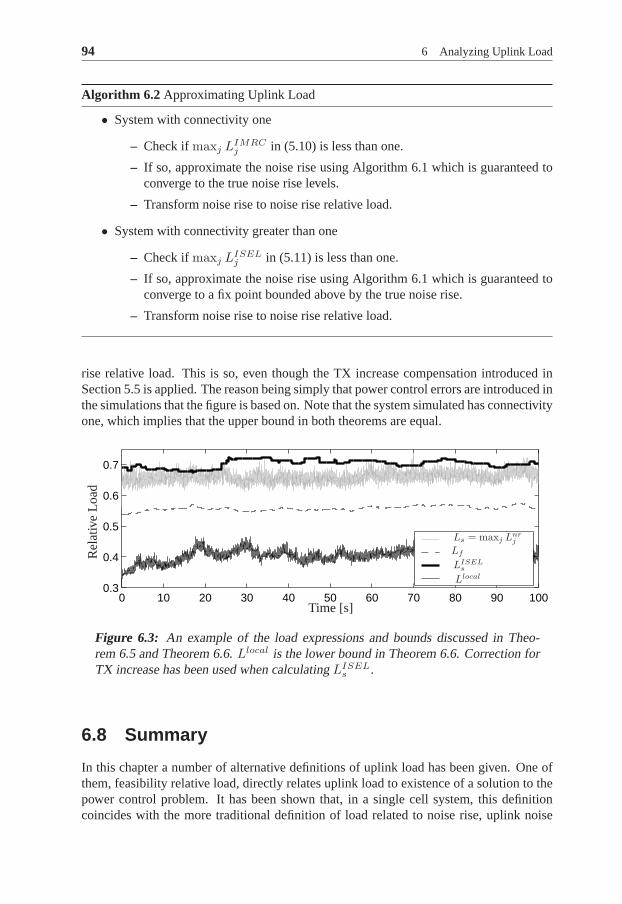
94 6 Analyzing Uplink Load
Algorithm 6.2 Approximating Uplink Load
• System with connectivity one
– Check ifmaxj LIMRCj in (5.10) is less than one.
– If so, approximate the noise rise using Algorithm 6.1 which is guaranteed toconverge to the true noise rise levels.
– Transform noise rise to noise rise relative load.
• System with connectivity greater than one
– Check ifmaxj LISELj in (5.11) is less than one.
– If so, approximate the noise rise using Algorithm 6.1 which is guaranteed toconverge to a fix point bounded above by the true noise rise.
– Transform noise rise to noise rise relative load.
rise relative load. This is so, even though the TX increase compensation introduced inSection 5.5 is applied. The reason being simply that power control errors are introduced inthe simulations that the figure is based on. Note that the system simulated has connectivityone, which implies that the upper bound in both theorems are equal.
0 10 20 30 40 50 60 70 80 90 1000.3
0.4
0.5
0.6
0.7
Time [s]
Rel
ativ
eLo
ad
LISELs
Ls = maxj Lnrj
Lf
Llocal
Figure 6.3: An example of the load expressions and bounds discussed in Theo-rem 6.5 and Theorem 6.6.Llocal is the lower bound in Theorem 6.6. Correction forTX increase has been used when calculatingLISEL
s .
6.8 Summary
In this chapter a number of alternative definitions of uplinkload has been given. One ofthem, feasibility relative load, directly relates uplink load to existence of a solution to thepower control problem. It has been shown that, in a single cell system, this definitioncoincides with the more traditional definition of load related to noise rise, uplink noise

6.8 Summary 95
rise relative load. However, in a general system they are different. Despite this, it hasbeen shown that expressions for uplink load derived in Chapter 5 can under somewhatidealistic circumstances be used to provide bounds on the rather theoretically orientedfeasibility relative load.
All expressions for uplink noise rise in Chapter 5 originatefrom a system of nonlinearequations. One way of solving these equations is to use iterations. The iterations are obvi-ously useful only if they converge to a stationary point. A number of sufficient conditionsfor existence of such a point was established in this chapter, and the point has been shownto be unique in case if the system has connectivity one. The analysis also showed that theconvergence point is the true noise rise level in case of a feasible system with connectivityone.

96 6 Analyzing Uplink Load
7Controlling Uplink Load
Resource controlis about assigning resources to the users. As such, it is a part of thesystem’s resource management. It is a delicate task, since not only must system feasibilitybe maintained while maximizing the resource utilization, there is also a trade off betweenfairness and capacity. Moreover, assigning resources to a user does not necessarily meanthat they will be used. For example, the user may not have enough transmission power tosupport the service or may not have any data to send.
These considerations imply that there are advantages with both centralized and decen-tralized resource control schemes, just as with load approximations. The reasons for thisare also pretty much the same. A central node has informationabout the situation in awider area and can therefore move resources from one area to another, while a local nodehas more accurate, detailed and up to date information on thelocal situation.
Partially as a motivation for the work in this chapter, the load approximations derivedin Chapter 5 are used for admission control. The performanceof the admission control us-ing the proposed load approximations is compared with usingan approximation based onthe intercell-to-intracell-interference factor. It is argued that the proposed load approxi-mations are easier to parameterize. For example, there is noneed to adapt any parametersto variations in the radio environment characteristics which is the case when using theintercell-to-intracell-interference factor. On the other hand, the centralized load approx-imations cannot adapt to fast changes in the radio environment, such as the multi pathfading. There is thus no way of mitigating any rapid load increase due to for example usermovement. A step towards solving this problem is obviously to use decentralized resourcemanagement. Following this introductory discussion, Section 7.2 gives a brief survey overdifferent ideas for solving the resource control problem presented in the literature.
The bulk of this chapter is in Section 7.3 and Section 7.4, where a number of re-source control algorithms are introduced and compared witheach other. Starting withcomplete knowledge of the radio environment and user requests in the entire network, acentralized resource control algorithm is introduced. This algorithm is not realistic since
97

98 7 Controlling Uplink Load
it requires far too much signaling, and is thus only meant forcomparison purposes. Re-alistic resource control algorithms making decisions in local nodes, using less and lessinformation about the surrounding radio environment, are then introduced.
One of the introduced reference algorithms is referred to asnoise rise controllingalgorithm. This is an example of a type of algorithms that is commonly found in theliterature. The algorithm uses no explicit information on the radio environment, such asusers’ relative power gain, but instead simply studies the uplink noise rise. It is shown inSection 7.5 that this type of algorithm easily suffers from unintentional shift in resourcesfrom one base station to another, or even decreased coverage, when using inaccurateknowledge of the background noise power. The chapter is finalized with a short summaryin Section 7.6.
The algorithms introduced in Section 7.3 were first presented and evaluated in (Gei-jer Lundin et al., 2005a). The basic idea which the algorithms are built on is filed in(Geijer Lundin and Gunnarsson).
7.1 Practical Centralized Resource Allocation
A number of uplink load approximations are derived and evaluated in Chapter 5. To closethe loop in Figure 1.1, these approximations will in this section be used as input to acentralized admission control algorithm, Algorithm 7.1.
Algorithm 7.1 Admission Control
Consider the next user in line for admissionAdmit the user if approximated load is still belowδAC in all base stationsafter having admitted the user.
The load approximation to be used has to be able to predict theload after havingadmitted a user. If the predicted load in any base station is above a parameterδAC , theuser is not admitted.
Seven different methods for approximating the uplink load will be used. The firstsix of these are derived in Chapter 5, the ones referred to asLIMRC , LISEL, LIBOTH ,LNMRC , LNSEL andLNBOTH . The seventh approximation is motivated by the discus-sion in Section 4.2.1 and is in cellj
Lrefj =
∑
i∈cj
(1 + f)βtgti
|Ki|,
where|Ki| is the number of cells that useri is connected to andf is the intercell-to-intracell interference factor.
For increased realism, an admission control decision does not take effect until onesecond after the decision is made. This is to model the latency in the connection setupbetween user and the central node in which the load approximations as well as the ad-mission decisions are made. A single service scenario with connectivity three offering a384 kbps service with target CIR ofβ0 = 0.14 is studied. The simulation area is coveredby 21 base stations at 7 different positions. The intercell-to-intrcell-interference factor in
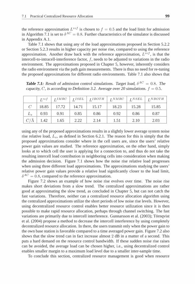
7.1 Practical Centralized Resource Allocation 99
the reference approximationLref is chosen tof = 0.5 and the load limit for admissionin Algorithm 7.1 is set toδAC = 0.8. Further characteristics of the simulator is discussedin Appendix A.1.
Table 7.1 shows that using any of the load approximations proposed in Section 5.2.2or Section 5.2.3 results in higher capacity per noise rise, compared to using the referenceapproximation. Another draw back with the reference approximation, Lref , is that theintercell-to-intracell-interference factor,f , needs to be adjusted to variations in the radioenvironment. The approximations proposed in Chapter 5, however, inherently considersthe radio environment via the path gain measurements. Thereis thus no need for re-tuningthe proposed approximations for different radio environments. Table 7.1 also shows that
Table 7.1: Result of admission control simulations. Target load,δAC = 0.8. Thecapacity,C, is according to Definition 3.2. Average over 20 simulations. f = 0.5.
Lref LIMRC LISEL LIBOTH LNMRC LNSEL LNBOTH
C 18.85 17.72 14.71 15.17 18.23 15.28 15.85
Ls 0.93 0.91 0.85 0.86 0.92 0.86 0.87
C/Λ 1.42 1.65 2.22 2.14 1.51 2.10 2.03
using any of the proposed approximations results in a slightly lower average system noiserise relative load,Ls, as defined in Section 6.2.1. The reason for this is simply that theproposed approximations consider where in the cell users are, since the users’ relativepower gain values are studied. The reference approximation, on the other hand, simplylooks at to which cell the user is applying for a connection to, and thus do not take theresulting intercell load contribution in neighboring cells into consideration when makingthe admission decision. Figure 7.1 shows how the noise rise relative load progresseswhen using three different load approximations. The approximations studying the users’relative power gain values provide a relative load significantly closer to the load limit,δAC = 0.8, compared to the reference approximation.
Figure 7.2 shows an example of how noise rise evolves over time. The noise risemakes short deviations from a slow trend. The centralized approximations are rathergood at approximating the slow trend, as concluded in Chapter 5, but can not catch thefast variations. Therefore, neither can a centralized resource allocation algorithm usingthe centralized approximations utilize the short periods of low noise rise levels. However,using decentralized resource control enables better resource utilization since it is thenpossible to make rapid resource allocation, perhaps through channel switching. The fastvariations are primarily due to intercell interference. Gunnarsson et al. (2003); Törnqvistet al. (2004) propose a method to decrease the intercell interference by using completelydecentralized resource allocation. In there, the users transmit only when the power gain tothe own base station is favorable compared to a time averagedpower gain. Figure 7.2 alsoshows that the slow trend can in fact increase almost2 dB in a matter of a second. Thisputs a hard demand on the resource control bandwidth. If these sudden noise rise raisescan be avoided, the average load can be chosen higher, i.e., using decentralized controlenables smaller margin to a maximum load level due to a smaller inter-sample time.
To conclude this section, centralized resource managementis good when resource

100 7 Controlling Uplink Load
0 200 400 600 800 1000 1200 1400 1600 1800 20000
0.2
0.4
0.6
0.8
1
Lref
LIBOTH
LNBOTHNoi
seR
ise
Rel
ativ
eLo
ad
Time, [s]
Figure 7.1: Noise rise relative load as a function of time when there is a one sec-ond delay between admission decision and transmission initialization (channel setupdelay).δAC = 0.8.
mobility between base stations is important. However, the load margins can be chosensmaller when using decentralized resource management due to the superior control band-width.
7.2 Resource Control Approaches
Resource control is about granting users access to resources in such a manner that boththe operator, who owns and operates the system, and the customers, who are users ofthe system, are satisfied with the performance. Typically, an operator wants as high athroughput as possible, and a user wants good coverage and high bit rates. To someextent, high bit rates are consistent with high throughput,but usually the throughput canbe increased by assigning resources to only one or a few usersin each cell. Even worse,increased coverage usually comes with decreased throughput. This trade off is the topicof Chapter 8.
Different views and proposed algorithms for regularly (re-)assigning resources to theusers will be discussed in this section.
Optimization Approaches Cellular radio systems of today support several services.This has made the resource control problem more complex. Oneway of solving thiscomplex problem is to mathematically express the quality ofservice (QoS) demands as autility function and fundamental requirements such as system feasibility as constraints inan optimization problem. The QoS demands can benetwork-centric, for example maxi-mizing the throughput as is done by Knopp and Humblet (1995) and Ulukus and Green-stein (2000), oruser-centricas in summarizing the users’ satisfaction. An example ofa user-centric strategy is given by Nagi et al. (2000) where they minimize users’ outageprobability. Further examples of where optimization has been used to solve the resourcecontrol problem are Rodriguez et al. (2004) and Sampath et al. (1995), who study a singlecell system.

7.2 Resource Control Approaches 101
1 2 3 4 5 6 7 8 9 10 11 12 13 14 15 16 17 18 193
4
5
6
7
8
9
10
Time [s]
Noi
seris
e,Λ
[dB
]
Figure 7.2: Example of noise rise. The grey plot is a time average of the the mo-mentarily noise rise (black). The momentarily noise rise has fast variations that canboth be avoided and taken advantage of by using decentralized resource control. Thesudden raises in average noise rise puts hard demands on the control bandwidth ofthe resource control.
Power and Rate Control Power control has been recognized as a powerful tool forincreasing system capacity. In fact, in CDMA cellular systems power control is crucialin order to overcome the near-far problem. However, while power control can compen-sate for deep fades in the channel between a user and the base station it is connected to,power control can also cause considerable intercell interference power peaks in neighbor-ing cells. One way of getting around this problem is to consider power and rate controljointly. Instead of increasing the transmission power, thetransmission rate can be de-creased. Duan et al. (2002); Hashem and Sousa (1998); Kim andLee (2000); Oh andWasserman (2003) and Kim and Honig (2000) use this idea.
Load Control Approaches In the border line between optimization and control, Jänttiand Kim (2001) use optimal control to solve a minimum time problem. The controlsignals are transmission powers that each user should send within each frame. The re-sults are derived under the assumption that the data rate is proportional to the carrier-to-interference ratio. The solution maximizes the throughputat each time instant.
Javidi (2003) solves an optimization problem using Lagrange multipliers. This leadsto a control problem aiming at a certain noise rise relative load. This is a truly decentral-ized solution in which each base station controls a cost for the users to connect to the basestation, higher cost means a smaller cell and less users.
Despite the absence of a central node, feasibility is guaranteed by Javidi (2003) throughthe use of a mutual agreement between the base stations. Thisidea is also used by Rezai-ifar and Holtzman (1999) and Feng et al. (2004). A drawback with the methods givenin the above references is that the local nodes require knowledge of the current receivedinterference power, which is generally considered hard to measure accurately.

102 7 Controlling Uplink Load
Opportunistic scheduling The idea here is to assign resources to the user with mo-mentarily best channel (Liu et al., 2001). This gives an unfair assignment on a short timescale. However, Berggren and Jäntti (2002) apply opportunistic scheduling in the down-link and show that it asymptotically provides the same fairness as a round robin scheduler,but with better utilization.
7.3 Resource Control Algorithms
As discussed in the introduction to this chapter, both centralized and decentralized re-source control schemes have its advantages. For example, using local resource controlalgorithms enables rapid assignment of resources based on local detailed knowledge con-cerning for example the radio channel or users’ momentarilytransmission requests. Whenusing a centralized resource control algorithm, on the other hand, it is much easier toachieve the soft capacity of the system since resources can easily be moved from one basestation to another. Obviously, knowledge of the situation in several base stations can beexplored in many other ways as well.
A number of resource control schemes that guarantee system feasibility are presentedin this section. When studying decentralized algorithms notusing a central node but yetguaranteeing system feasibility, it will be shown that system capacity can be increasedby studying information about the users’ relative power gain, compared to studying thecorresponding power gain values. Furthermore, a resource control algorithm using botha central node and local nodes will be introduced. The idea isto take advantage of bothcentralized and decentralized schemes. The algorithms arepresented in such an orderthat they have less and less information on the surrounding radio environment. Startingwith a centralized algorithm and ending with the noise rise controlling algorithms usingas coarse information as which base station users are connected to.
Algorithms not studying relative power gain values but instead maintain feasibilityby looking at measurements of uplink noise rise will also be studied. Characteristics ofthis kind of algorithms is studied in Section 7.5 through a theoretical study in a simpli-fied scenario as well as a more practical approach using simulations. As relatively hightarget CTIR values will be studied here, the degradation in performance due to self inter-ference can no longer be neglected. Recalling the relation between CTIR, CIR and selfinterference in (3.7),
γ =C
Itot − (1 − α)C=
β
1 − (1 − α)β.
Furthermore, the resource control algorithms will be posedas optimization problems. Theutility function in these optimization problems will oftenbe the system capacity accordingto Definition 3.2. For notational ease, introduce
κ(βtgt, α) =
M∑
i=1
log2
1 + αβtgti
1 − (1 − α)βtgti
for the system capacity when users have target CTIR values according to the vectorβ ∈R
M and the self interference factor isα.

7.3 Resource Control Algorithms 103
A final remark before introducing the resource control algorithms is that the eigen-value corresponding to the spectral radius of a positive matrix, i.e., a matrix with onlypositive elements in it, is positive and real. See Appendix A.2.
7.3.1 Centralized Robust Algorithm
In this section a completely centralized algorithm will be introduced. The algorithm willbe used as an upper bound on the capacity. As such it is provided with power gain infor-mation from the entire system.
Ideally, the users would be given target CTIR values according to the solution to
maximizeβtgt
i
κ(βtgt, α)
s.t.L 4 LtgtE,(7.1)
where the utility function is the system capacity and the constraint simply states thatthe maximum eigenvalue ofL must be less than the scalar parameterLtgt, i.e., λ(L) ≤Ltgt < 1. This corresponds to the feasibility relative load also being less thanLtgt.
The tools used for solving the optimization problems (Löfberg, 2004; Toh et al., 2001)can only solvelinear matrix inequalities(LMI) involving symmetric matrices. Therefore,the constraint in (7.1) can not be considered explicitly. However, using the Schur com-plement, see Appendix A.3, the LMI in (7.1) can be substituted by
(E L
LT Ltgt2E
)
� 0.
This constraint corresponds to requiring the maximum singular value ofL to be less thanor equal toLtgt squared. As the spectral radius of a matrix is always less than the squareroot of the maximum singular value, the constraint is harderthan that in (7.1).
Substituting the constraint in (7.1) with the above LMI yields Algorithm 7.2.
Algorithm 7.2 Centralized RRA Algorithm
Assign target CTIR values according to the solution to
maximizeβtgt
i
κ(βtgt, α)
s.t.
(E L
LT Ltgt2E
)
� 0.(7.2)
7.3.2 Semi-Centralized Robust Algorithm
Ways of providing more resources to some base stations and less to others include usinga central node or communication between the base stations. Aresource controlling algo-rithm using a central node as well as local nodes is proposed in this section. The centralnode will hand out resource pools to the local nodes hosted inthe base stations. The

104 7 Controlling Uplink Load
algorithms in the base stations can then use these pools while respecting a mutual agree-ment between the base stations and the central node. The mutual agreement is crucial toguarantee system feasibility.
Resources are distributed among the base stations through the use of information feedback from the base stations to the central node. The information fed back will be abouthow many and where the users are located. However, due to limited bandwidth betweenbase stations and the central node, it is not tractable to send too much information.
Figure 7.3 shows a schematic view of the information flow in the algorithm proposedhere. The main idea is to limit the intercell interference byconsidering the relative power
Central node
Local nodes
s1
s2
sB
γtgti , i ∈ c1
γtgti , i ∈ c2
γtgti , i ∈ cB
Y (limited information)
Figure 7.3: Information flow in a decentralized RRM algorithm. The central nodehands out resource pools,sk, to the local nodes. The local nodes distribute resourcesto the users in form of target CIR values and also provide feedback to the centralnode.
gains,zi,j . The element on rowk and columnj in the system matrixL is at timet
Lk,j(t) =∑
i∈ck
βtgti (t)zi,j(t).
This number can be interpreted as the noise rise relative load caused by cellk in cell jor, more accurately put,Lk,jI
totk is the intercell interference power users in base station
k introduce in base stationj. Thus, limiting the off diagonal elements of the systemmatrix corresponds to limiting the intercell interference. By assigning users with higherrelative power gain to neighboring base stations smaller target CTIR values, each term inthe elements of the system matrix can be made small without decreasing system capacity.
The resource controlling algorithm is an implementation ofthe lemmas that follownext. System feasibility is guaranteed by meeting the requirements in these lemmas. The

7.3 Resource Control Algorithms 105
information fed back to the central node by base stationk is at timet
Yk,j(t)△
=1
∑
i∈ckβtgt
i (t − 1)
∑
i∈ck
βtgti (t−1)zi,j(t−1) =
1∑
i∈ckβtgt
i (t − 1)Lk,j(t−1).
(7.3)The normalizing gives a nice interpretation of the variables sent from the central node tothe local nodes as resource pools.
Introduce the matrixL = [Lk,j ] as
Lk,j△
= sk(t)Yk,j(t),
wheresk is a scalar. Eachsk will later be interpreted as a resource pool given by thecentral node to base stationk, see Figure 7.3.
Lemma 7.1If
Lk,j(t) ≤ Lk,j ∀k, j ∈ {1, B}, (7.4)
andλ(L) ≤ Ltgtf thenλ(L) ≤ Ltgt
f .
Proof: Follows from the fact that increasing an element of a positive matrix can notdecrease its maximum eigenvalue.
The inequality in Lemma 7.1 will be used as a mutual agreementbetween the centralnode and local nodes.
Lemma 7.2If
(
E L
LT Ltgtf
2E
)
� 0, (7.5)
whereE is the identity matrix of appropriate dimension, thenλ(L) ≤ Ltgtf .
Proof: See Appendix A.7.
Combining Lemma 7.1 and Lemma 7.2 yields the following theorem.
Theorem 7.1A system using a resource control algorithm that meets the inequalities in(7.4)and (7.5)is feasible ifLtgt
f is less than one.
Proof: As the requirement in (7.5) is met,λ(L) ≤ Ltgt. According to Lemma 7.1,λ(L) is then also less thanLtgt if the inequality in (7.4) is met. Finally, according toTheorem 6.2, this yields feasibility ifLtgt is chosen less than one.
With the assumption that eachLk,j(t) is smaller than or equal toLk,j , the central nodeassigns resource poolssk(t) according to the solution to optimization problem (7.6).

106 7 Controlling Uplink Load
maximizes(t)
U(s(t))
s.t.
(
E L
LT Ltgtf
2E
)
� 0,
Lk,j = skYk,j , k, j = 1, 2, . . . , B.
sk(t) =∑
i∈ckβtgt
i (t)
βmin ≤ βtgti (t) ≤ βmax, i = 1, 2, . . . ,M.
(7.6)
As utility function, U(s), one should choose a concave function as this makes (7.6) aconvex problem according to Boyd and Vandenberghe (2004). Apossible choice is agreedy version
Ug(s(t))△
=
B∑
k=1
sk(t), (7.7)
which simply maximizes the combined resource pool or, in order to promote fairness forusers in crowded cells, one can choose
Uf (s(t))△
=
B∑
k=1
Mksk(t), (7.8)
whereMk is the number of users connected to base stationk. Obviously other choices ofutility function can be made. The simulations reported on inSection 7.4 useUf .
Now, consider the local nodes. Their task is to assign targetCTIR values such thatthe constraint in (7.4) is indeed met. By combining the resource poolsk(t) and the valuethey fed back to the central node,Yk,j(t), they can calculate the upper bound in (7.4) ontheir own. Local nodek will choose the target CTIR values at timet according to theoptimization problem in (7.9).
maximizeβtgt
i(t)
κ(βtgt(t), α)
s.t.
{∑
i∈ckβtgt
i (t)zi,j(t) ≤ Yk,j(t)sk(t)∀j
βmin ≤ βtgti (t) ≤ βmax,∀i ∈ ck.
(7.9)
Note that the requirement that the combined target CTIR values must be less than orequal tosk in base stationk, is handled by the first constraint whenj = k. If the firstconstraint is respected in all base stations, each element of L is indeed upper bounded bythe corresponding element inL, i.e., the inequality in (7.4) is met. The utility functionis in this case the base station capacity. Again, of course one can think of other utilityfunctions, for example promoting fairness over capacity.
The resource control scheme introduced in this section is summarized in Algorithm 7.3.Using the iterative procedure yields that users who are not assigned any resources will notaffect the values send back to the central node. Furthermore, the iterations improve thealgorithm’s ability to adapt to resource demands moving from one base station to another.

7.3 Resource Control Algorithms 107
Algorithm 7.3 Semi-Centralized RRA Algorithm
1. Given an initial matrixY (t)
2. The central node assigns each base station a resource pool, sk(t), k = 1, 2, . . . , B,according to the solution to problem (7.6).
3. Each base stationk chooses target CTIR values,βtgti (t) ∈ ck, according to the
solution to problem (7.9).
4. Each base stationk calculates new valuesYk,j(t + 1), j = 1, 2, . . . , B to be sendto the central node.
5. Increase the time indext, t = t + 1.
6. Continue from point 2 above.
Remark7.1. An interpretation ofsk(t) as a resource pool is given by studying (7.4) whenAlgorithm 7.3 has reached a steady state. For the special case whenk = j, i.e., on thediagonal ofL (note thatzi,Ki
= 1∀i),
Lk,k =∑
i∈ck
βtgti zi,k =
∑
i∈ck
βtgti ≤ Lk,k = sk.
The scalarssk(t) is thus an upper bound on the sum of the target CTIR values of usersconnected to base stationk.
7.3.3 Decentralized Robust Algorithms
A result applicable to all matricesL is
λ(L) ≤ ||L||∞,
whereλ(L) is the maximum eigenvalue ofL (Skogestad and Postlethwaite, 1996, page520). In the special case of positive matrices, the right hand side of the above inequalityis simply the maximum row sum. Using this fact, we can prove the following theorem.
Theorem 7.2 (Local Robustness)If users in a system with connectivity one are assigned resources in such a manner that
B∑
j=1
Lk,j ≤ Ltgtf , ∀ k
then the feasibility relative load is less than or equal toLtgtf .
Proof: For positive matricesL ∈ RB×B ,
λ(L) ≤ ||L||∞ = maxk
B∑
j=1
Lk,j .

108 7 Controlling Uplink Load
Furthermore, according to Theorem 6.2, the feasibility relative load in a system withconnectivity one isλ(L). Hence, if all row sums ofL are less than or equal toLf , somust the feasibility relative load be.
A result given by (Gantmacher, 1974, page 63) is applicable to positive matrices andstates that the maximum eigenvalue is bounded from below by the minimum row sum.Hence, the upper bound in Theorem 7.2 may not be very conservative. It is even equalityif all row sums equalLtgt
f .
Remark7.2. Theorem 7.2 is similar to Corollary 6.1. The only differenceis that The-orem 7.2 uses row sums of the system matrixL and Corollary 6.1 uses column sums.This corresponds to taking sums over the load a base stationscauses and the load a basestations experiences, respectively. A result is thus that the system is feasible if either sumis less than or equal to unity.
Theorem 7.2 can be used to design a local resource control algorithm in which eachbase station assigns resources to the users connected to it.Since one base station controlsa whole row in the system matrix, it can assign resources suchthat the corresponding rowsum is always less thanLtgt
f .The sum over elements on rowk in the system matrix is
B∑
j=1
Lk,j =
B∑
j=1
∑
i∈ck
βtgti zi,j =
∑
i∈ck
βtgti
B∑
j=1
zi,j . (7.10)
An interesting observation from a practical point of view, is that if the relative power gains,zi,j , are not already available in the local nodes all that the central node needs to provideis the relative power gain sum over base stations in (7.10). This means a considerablereduction in signaling between central and local nodes, compared to sending each users’relative power gain to the base stations.
Two different scenarios are considered in different paragraphs below. In them, boundson the sum of users’ target CTIR values are derived with and without information aboutthe users’ relative power gain values.
Not Using Relative Power Gain Information If information on the users’ relativepower gain to other base stations is not used, robustness canstill be achieved by assumingthat these relative power gains are less than somezmax
1,i.e.,
zi,j < zmax, j 6= Ki.
Now, the constraint in Theorem 7.2 yields an upper bound on the sum of the users’ targetCTIR in each cell,
B∑
j=1
Lk,j =∑
i∈ck
βtgti
B∑
j=1
zi,j ≤∑
i∈ck
βtgti (1 +
∑
j 6=k
zmax) ≤ Ltgtf ⇒
sk =∑
i∈ck
βtgti ≤
Ltgtf
1 + (B − 1)zmax,
1That the relative power gains to other base stations are in fact less thenzmax has to be guaranteed by someother means in this case.

7.3 Resource Control Algorithms 109
wheresk can be thought as aresource poolthat base stationk may split arbitrarily amongthe users connected to it. Algorithm 7.4 explains a resourcecontrol algorithm using thisidea.
Algorithm 7.4 Power Gain Based Local RRA Algorithm
Each base stationk assigns target CTIR values to the users inck according to the solutionto the following optimization problem.
maximizeβtgt
i
κ(βtgt, α)
s.t.
{∑
i∈ckβtgt
i ≤ Ltgt
f
1+(B−1)zmax
βmin ≤ βtgti ≤ βmax,∀i ∈ ck.
(7.11)
Note that the sum of users’ target CTIR in the whole system is upper bounded by
B∑
j=1
sj ≤ BLtgt
f
1 + (B − 1)zmax.
As the number of base stations,B, tends to infinity this upper bound tends toLtgtf /zmax.
Using Relative Power Gain Information By looking at the expression in (7.10), wecan conclude that users with high relative power gain to other base stations should begiven smaller target CTIR values. Algorithm 7.5 uses this idea. The only difference be-
Algorithm 7.5 Relative Power Gain Based Local RRA Algorithm
Each base stationk assigns target CTIR values to the users inck according to the solutionto the following optimization problem.
maximizeβtgt
i
κ(βtgt, α)
s.t.
{∑
i∈ckβtgt
i
∑Bj=1 zi,j ≤ Ltgt
f
βmin ≤ βtgti ≤ βmax,∀i ∈ ck.
(7.12)
tween Algorithm 7.4 and Algorithm 7.5 is in the constraints.The feasible region of theoptimization problem considered in Algorithm 7.5 is largerthan that in Algorithm 7.4sincezi,j ≤ zmax. The former will therefore provide a capacity at least as high as Al-gorithm 7.4 will. Another way of looking at it is that Algorithm 7.4 assumes that allusers stand in the worst position possible, and must therefore be more conservative thanAlgorithm 7.5.
By looking at the constraints in (7.12), the cost for assigning resources to a user isproportional to the user’s sum over relative power gain values. Therefore, as a user’s con-tribution to the total capacity only depends on its target CTIR, the user with lowest relativepower gain sum will be assigned the highest target CTIR when using Algorithm 7.5.

110 7 Controlling Uplink Load
7.3.4 Blind Algorithms
For comparison reasons, two more algorithms will be introduced. These algorithms areblind in the sense that they will not consider the users’ power gain values, but merely towhat base station the users are connected to.
Noise Rise Controlling Algorithm A straightforward way of implementing decen-tralized resource management by controlling the uplink noise rise. To exemplify, Algo-rithm 7.6 is an implementation of this idea. It is common to use a noise rise controlling
Algorithm 7.6 Noise Rise Controlling Algorithm
For each base stationk and each time step
1. Establish the uplink noise rise.
2. Assign target CTIR values,βtgti ∈ [βmin, βmax]∀i ∈ ck while aiming at a noise
rise ofΛtgt.
algorithm for local resource management, see for example the work done by Damnjanovicet al. (2002); Neubauer and Bonek (2001) or Javidi (2003). A basic requirement for usingsuch an algorithm is obviously that the uplink noise rise canbe made available throughmeasurements of the uplink interference power or in some other way, e.g., using the ap-proximations in Chapter 5.
While this simple idea guarantees system feasibility, it suffers from other weaknesses.One of these is that resources can be unintentionally shifted between base stations. Thisproblem is studied in Section 7.5.
Cell Based Algorithm Algorithm 7.7 is inspired by with what is done in an additionto the uplink in WCDMA called Enhanced UplinkParkvall et al. (2005). The algorithmuses fixed resource pools,sk = s0. The constants0 is a design parameter which shouldbe chosen with consideration taken to the amount of intercell interference and the tradeoff between system capacity and probability of assign resources corresponding to an infeasible system. Since the algorithm does not consider the radio environment more thanto which base station users are connected to, it can not guarantee system feasibility. Whensetting the resource pool, the intercell-to-intracell-interference factor can be considered.A higher expected intercell-to-intracell-interference factor can be handled with choos-ing a smaller resource pool,s0. In a sense, this algorithm is the opposite of the com-pletely centralized algorithm, Algorithm 7.2. The algorithm is user-centric as opposedto network-centric since it assign equal resources to all users connected to the same basestation. Most important, though, is that Algorithm 7.7 doesin no way guarantee systemfeasibility.

7.4 Resource Control Evaluations 111
Algorithm 7.7Assume a target intra-cell load ofs0 in each cell.
1. Abort without solution if any
s0
|ck|< βmin, k = 1, 2, . . . , B.
Here,|ck| is the number of users connected to base stationk.
2. Assign each useri connected to base stationk a target CTIR of
βtgti = min
(s0
|ck|, βmax
)
.
7.4 Resource Control Evaluations
Three of the algorithms introduced in Section 7.3 will here be evaluated and comparedwith a rather simple resource controlling algorithm. The algorithms from the previoussections that will be evaluated are
• Algorithm 7.2, which is a completely centralized algorithm
• Algorithm 7.3, which uses both a central node and local nodes
• Algorithm 7.5, which is a decentralized algorithm using independent local nodes
• Algorithm 7.6, which uses knowledge of the uplink noise rise
• Algorithm 7.7, which is a decentralized algorithm
The first three algorithms have in common that they all guarantee a feasible resource con-trol if they are provided with accurate power gain measurements. Algorithm 7.6 studiesthe noise rise and thereby guarantee system feasibility, but all users in a cell will be as-signed equal target CTIR. No attempts to minimize the intercell interference will thus bemade by the algorithm. Algorithm 7.7 does not take any consideration to the intercellinterference nor the noise rise level, so system feasibility is therefore not guaranteed.
Two different scenarios will be simulated. The users are spread over the simulationarea using a uniform distribution in the first scenario. In the second scenario, a big partof users are concentrated to small area. This will produce high load in some base stationsand less load in the surrounding ones.
The simulation area consists of 9 base stations grouped intothree different positions.The cell diameter is 750 meters and the attenuation exponentis α = −3.52. After one ofthe resource control algorithms has assigned target CTIR values to the users, the valuesare adjusted to compensate for limited transmission power.The users’ maximum trans-mission power ispmax = 21 dBm. In this simple study, only static simulations have beenused, i.e., no user movement or power control has been simulated. This corresponds toassuming perfect power control and as fast a resource control that the changes in radio

112 7 Controlling Uplink Load
environment due to user movement can be neglected. The users’ power gain values aretaken from the simulator explained in Appendix A.1. Furthermore, Löfberg (2004) andToh et al. (2001) were used to solve the optimization problems in the algorithms.
The impact of self interference can be neglected if the target CTIR can be assumedsmall, as Figure 3.4 suggests. As opposed to earlier work in for example Chapter 5, largetarget CTIR will be studied here, which is why self interference will be considered in thesimulations. The self interference factor is chosen toα = 0.1.
For increased statistic accuracy, 50 Monte Carlo simulations are used for each loadlevel. The minimum and maximum target CTIR values are chosento βmin = −15 dBandβmax = 0.5, respectively.
The result of the semi-centralized algorithm, Algorithm 7.3, depends on the initialmatrixY . For the purpose of calculating the initial information to feed back to the centralnode, introduce
ij△
= arg mini∈cj
∑
k
zi,k.
The initial Y is calculated using (7.3) with all users target CTIR equal toβmin exceptuserij in each cellj who is instead given a target CTIR ofβmax. This choice of initialtarget CTIR values is influenced by the way resources are chosen by Algorithm 7.5.
Uniformly distributed users Figure 7.4a and Figure 7.4b show the system capacityand the variance of the users’ target CTIR values as a function of the maximum noise rise,where
maximum noise rise= maxj
Λj .
It is clear from the plots that the algorithms studying the users’ relative power gain per-form better from a network centric perspective. However, the usual trade off betweencapacity and fairness, or between network and user centric objectives, is apparent whenlooking at the middle plot. The users’ target CTIR variance is considerably smaller whenusing either of the reference algorithms, Algorithm 7.6 or Algorithm 7.7, indicating thatthese algorithms promote fairness more than the algorithmsoptimizing the system capac-ity.
All three algorithms studying the users’ relative power gain provide approximatelyequal performance in terms of capacity and fairness. This means that Algorithm 7.5,which does not use a central node at all, provides the same capacity as the completelycentralized algorithm. However, as Figure 7.4c shows, Algorithm 7.5, is not as goodas the other two robust algorithms to find a feasible solution. The plot indicates thatAlgorithm 7.3 in fact manages to move resources around to finda feasible solution evenfor small values of the maximum allowed feasibility relative load. It is therefore likelythat Algorithm 7.3 is better at finding a feasible solution for a fixed maximum allowedfeasibility relative load as the offered load grows, compared to Algorithm 7.5.
Non-Uniformly distributed users In this scenario, the users are located at positions{x, y} which are both distributed according to a bimodal distribution consisting of a Gaus-sian and a uniform distribution. In meters, the distribution is
0.3N (0, 300) + 0.7U [−2000, 2000].

7.5 Inaccurate Background Noise Power Knowledge 113
0 1 2 3 4 5 6 7 8 9 100
5
10
0 1 2 3 4 5 6 7 8 9 100
0.1
0.2
0.2 0.3 0.4 0.5 0.6 0.7 0.8 0.9 10
0.5
1
a)
b)
c) maxj Λj
maxj Λj
Cap
acity
var(
βtg
ti
)
Maximum allowed feasibility relative load
P(s
ucce
ss)
Algorithm 7.7
Algorithm 7.3Algorithm 7.5
Algorithm 7.2
Algorithm 7.6
Figure 7.4: Simulation results when users are uniformly distributed.βmin =−15 dB, βmax = 0.5, α = 0.1
This gives an area with considerably higher user density. This scenario is one wherethere is performance to gain from moving resources from the low user density area tothe high density area. This can be done by i.e., Algorithm 7.2and Algorithm 7.3 butby the decentralized robust algorithm, Algorithm 7.5. The former two have a centralnode that can distribute resources between different base stations. Figure 7.5 indicatesthat these algorithms are indeed capable of moving resources to the highly loaded cellsince, compared to the local robust algorithm, they more often find a feasible solution asshown in Figure 7.5c. Note that the Algorithms proposed in Section 7.3 and studied here,will either produce a feasible resource assignment or no result at all. This means that itis possible to in advance detect an overload situation and take necessary actions beforetrying to make an infeasible resource assignment leading toperformance losses.
7.5 Inaccurate Background Noise Power Knowledge
The current section is devoted to evaluating how inaccurateinformation on the uplinknoise rise affects the system capacity when Algorithm 7.6 isused in the base stations. Inthe specific scenario studied, the uplink noise rise is established by measuring the uplinkinterference power and dividing by the background noise power. A problem with this

114 7 Controlling Uplink Load
0 1 2 3 4 5 6 7 8 9 100
5
10
0 1 2 3 4 5 6 7 8 9 100
0.1
0.2
0.2 0.3 0.4 0.5 0.6 0.7 0.8 0.9 10
0.5
1
a)
b)
c) maxj Λj
maxj Λj
Cap
acity
var(
βtg
ti
)
Maximum allowed feasibility relative load
P(s
ucce
ss)
Algorithm 7.7
Algorithm 7.3Algorithm 7.5
Algorithm 7.2
Algorithm 7.6
Figure 7.5: Simulation results when 30 % of the users are concentrated toa smallarea.βmin = −15 dB, βmax = 0.5, α = 0.1
technique is that it is hard to measure the background noise power. Inaccurate knowledgeof the background noise power leads to inaccurate information about the noise rise.
Let thebackground noise power ratio, θj , be the ratio between true and a nominalbackground noise power in cellj, i.e.,
θj△
=Nj
N0⇒ Nj = θjN0, (7.13)
whereN0 is a nominal background noise power common to all cells. Using an estimateof the background noise power ratio,θj , and accurate measurements of the uplink inter-ference power, the uplink noise rise in cellj can be estimated as
Λj =Itotj
θjN0
=θj
θj
Λj .
The ratio between true and estimated noise rise is thus
ρj△
=Λj
Λj
=θj
θj.

7.5 Inaccurate Background Noise Power Knowledge 115
0 0.5 1 1.5 2 2.5 30
0.5
1
1.5
2
2.5
3
ρ1
Cap
acity
log2(1 + γ1)log2(1 + γ2)∑
log2(1 + γi)
Figure 7.6: Capacity’s dependence on inaccurate information on background noisepower.Λmax = 6 dB, z1,2 = 0.4, z2,1 = 0.6, α = 0.1, ρ2 = 1, N1 = N2.
The aim of this section is to study how the base station capacities change as theρ valuesin the different base stations deviate from one.
A ρj < 1 corresponds toΛj < Λj , i.e., the true noise rise is lower than what theresource assigning algorithm thinks. This causes a decrease in resource utilization in cellj. Exactly how much the capacity is decreased will be studied in two examples below.
Example 7.1Consider a system consisting of just two base stations, or likewise, assume that two basestations can be isolated from the remaining system. For presentational ease, it is assumedthat only one user at a time in each cell is transmitting, userone in cell one and user twoin cell two. Consider a noise flat system with connectivity one. Solving for the uplinkinterference power in (6.1) and dividing by the common background noise power resultin a matrix expression according to
(Λ1
Λ2
)
=
(11
)
+
(Λ1 Λ2z2,1
Λ1z1,2 Λ2
)(β1
β2
)
.
Now, if the local noise rise controlling algorithm in base station j aims at an estimatednoise rise ofΛmax, the true noise rise will beΛj = Λmaxθj/θj = ρjΛ
max. The abovematrix expression can under these assumptions be written as
Λmax
(ρ1
ρ2
)
=
(11
)
+ Λmax
(ρ1 ρ2z2,1
ρ1z1,2 ρ2
)(β1
β2
)
. (7.14)
Figure 7.6 shows the capacity of the two base stations as wellas the sum of the capacitiesas function ofρ1 whenρ2 = 1. When solving (7.14) above, the natural constraints that0 ≤ βi ≤ 1 has been taken into account. If the solution to (7.14) implies aβi < 0, asingle cell scenario is studied instead, i.e., the cell withβi < 0 will be omitted.
Naturally, the capacity in cell one increases withρ1, which is also apparent in Fig-ure 7.6. This gain in capacity in cell one comes with decreased capacity in the neighboringcell. A too lowθ1 will lead to loss in coverage since cell one is effectively not providingany service at all. For example whenρ1 < 0.55, γ1 = 0 because the base station thinksthat the intercell interference causes aΛ1 > Λmax. Conversely, a too highρ1 leads toabsence of service in cell two.

116 7 Controlling Uplink Load
0 0.5 1 1.5 2 2.5 30
0.5
1
1.5
2
ρ1
Cap
acity
C1C2C1 + C2
Figure 7.7: Capacity’s dependence on inaccurate information on background noisepower. The capacity in base stationj is denotedCj . Λmax = 6 dB,α = 0.1, ρ2 = 1,N1 = N2.
Behavior of the base station capacities in Example 7.1 with specific choices of relativepower gain values and only one user in each cell can be generalized. Clearly, underes-timating the background noise power, i.e.,ρ < 1, corresponds to a capacity loss in theown cell, but other cells experience lower intercell interference. The total system capacitymay thus not decrease in the general case, but resources willdefinitely be transferred be-tween cells. Conversely, overestimating the background noise power, i.e.,ρ > 1, leads toincreased capacity in the own cell also since it correspondsto underestimating the noiserise yielding a true noise higher thanΛmax. A significant error, such asρ < 0.5 corre-sponding to under estimating the background noise power with 3 dB, will certainly causean unintentional shift of resources between the base stations. Example 7.2 shows an ex-ample of how the resources are shifted when considering several users in each cell.
Example 7.2
Consider a noise flat system with two base stations. The same calculations as were donein Example 7.1 can be used to consider several users in each base station. As opposed toExample 7.1, simulations are this time used. In each of the 50performed Monte Carlosimulations, 40 users are spread over an area between the twobase stations. The path gainmodel in the simulator described in Appendix A.1 is used. To simplify the calculations,all users in the same base station will be assigned the same target CTIR,sj , j = 1, 2.
Figure 7.7 shows how resources are transferred from base station two to base stationone asρ1 increases. As long asρ1 is small, increasedρ1 also yields higher total capacity.However, too high values ofρ1 implies that the capacity loss in base station two is biggerthan the capacity increase in base station one yielding a loss in total capacity.
The example indicates that it is important to have accurate knowledge of the back-ground noise power, otherwise capacity is unintentionallytransferred between base sta-tions and the total capacity is decreased in general.

7.6 Summary 117
7.6 Summary
Simulations indicate that using knowledge about the users’relative power gain values en-ables better resource control. Both when using centralizedand decentralized algorithms.In the case of centralized control, the load approximationsstudied in Chapter 5 wereused for admission control. By choosing users with a more favorable radio environment,higher capacity can achieved with the same noise rise compared to when using a loadapproximation not considering the users’ radio environment.
However, due to the slow update rate and the latency in performing the resource man-agement decisions, a completely centralized solution is not appealing in practice. Instead,a degree of decentralization should be introduced in order to better adapt and take advan-tage of a changing radio environment. Two algorithms that make local resource manage-ment decisions were proposed, one that uses a central node todistribute resources overdifferent base stations and one algorithm that does not havea central node at all. A sim-ulation study of the performance of the algorithms implied that considering the relativepower gain in the resource allocation gives better performance compared to only studyingwhich base station the users are connected to. More importantly, the algorithms usingrelative power gain either produce a feasible resource assignment or no assignment at all.This means that it is possible to, in advance, decide if the resource demands are too high.
A conceptual study of a group of decentralized resource control algorithms, here re-ferred to as noise rise controlling algorithms, was introduced. These algorithm can, in away, be seen as the opposite to the practical centralized algorithms since they only studythe uplink noise rise in the own cell. The evaluation showed that neither these algorithmsare well suited for practical usage due to a possible unintentional shift of resources. Thisshift may lead to increased capacity in a few base stations but will definitely imply de-creased coverage or even lack of service in other.

118 7 Controlling Uplink Load

8Feasibility versus Coverage
Load has always been related to system feasibility in the previous chapters. It has alwaysbeen a question on whether or not the system is feasible. Thischapter focuses on the loadlevel’s impact on the relation between performance measures such as coverage, capacityand users’ individual service quality. This trade off is touched upon in Section 4.1, whenmotivating the definition of noise rise relative load. The analysis in this chapter leads toa discussion on how to set the target values of the resource control algorithm in differentsystem deployments.
Section 8.1 studies a scenario where the users have unlimited transmission power.It is concluded that there is a trade off between signal quality and cell size in a multicell system where the users interfere with each other, even with unlimited transmissionpowers. The type of limitations is also put in a system deployment perspective.
A user transmission power limitation has been applied in Section 8.2. This implies adifferent dependence on the users power gain distribution.A stochastic approach to linkbudgets is adopted. This leads to guide lines for choosing the maximum uplink noiserise relative load as a function of the background noise power in systems with large cells.Results of the link budgets are also used as input to a discussion about what quantitiesare important in different system deployments, when the users’ transmission powers arelimited.
The two different scenarios, with and without transmissionpower limitations, arecombined in a discussion on how to choose the target load level for resource managementalgorithms in Section 8.3.
Results presented in this chapter are partially given in (Geijer Lundin et al., 2005b).
119
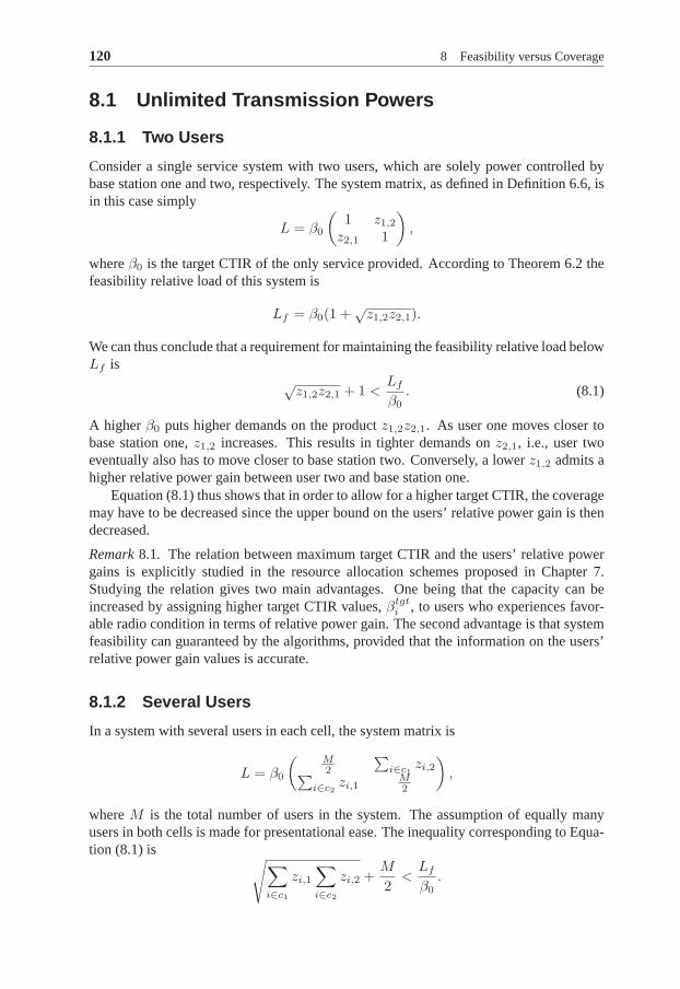
120 8 Feasibility versus Coverage
8.1 Unlimited Transmission Powers
8.1.1 Two Users
Consider a single service system with two users, which are solely power controlled bybase station one and two, respectively. The system matrix, as defined in Definition 6.6, isin this case simply
L = β0
(1 z1,2
z2,1 1
)
,
whereβ0 is the target CTIR of the only service provided. According toTheorem 6.2 thefeasibility relative load of this system is
Lf = β0(1 +√
z1,2z2,1).
We can thus conclude that a requirement for maintaining the feasibility relative load belowLf is
√z1,2z2,1 + 1 <
Lf
β0. (8.1)
A higherβ0 puts higher demands on the productz1,2z2,1. As user one moves closer tobase station one,z1,2 increases. This results in tighter demands onz2,1, i.e., user twoeventually also has to move closer to base station two. Conversely, a lowerz1,2 admits ahigher relative power gain between user two and base stationone.
Equation (8.1) thus shows that in order to allow for a higher target CTIR, the coveragemay have to be decreased since the upper bound on the users’ relative power gain is thendecreased.
Remark8.1. The relation between maximum target CTIR and the users’ relative powergains is explicitly studied in the resource allocation schemes proposed in Chapter 7.Studying the relation gives two main advantages. One being that the capacity can beincreased by assigning higher target CTIR values,βtgt
i , to users who experiences favor-able radio condition in terms of relative power gain. The second advantage is that systemfeasibility can guaranteed by the algorithms, provided that the information on the users’relative power gain values is accurate.
8.1.2 Several Users
In a system with several users in each cell, the system matrixis
L = β0
(M2
∑
i∈c1zi,2
∑
i∈c2zi,1
M2
)
,
whereM is the total number of users in the system. The assumption of equally manyusers in both cells is made for presentational ease. The inequality corresponding to Equa-tion (8.1) is
√∑
i∈c1
zi,1
∑
i∈c2
zi,2 +M
2<
Lf
β0.

8.2 Limited Transmission Powers 121
The above inequality must be respected if the feasibility relative load is to be maintainedbelow Lf . However, the constraint can be met in many different ways. For example,providing service to more users can be compensated for by decreasing the target CTIR,increasing the possible feasibility relative load or assigning service only to users withsmall relative power gain.
In for example systems with small cells, where the users’ power gain values are rel-atively large, it is likely that the above inequality is in fact what limits the performancealso with limited user transmission powers. The above expression not only confirms thewell known fact that a dense deployment yields a capacity limited system, as opposed tocoverage limited, but the expression also provides a requirement on properties directlyrelated to coverage, capacity and quality of users’ service.
8.2 Limited Transmission Powers
In the presence of limited user transmission power, coverage depends on the amount ofreceived interference power at the base station antenna. This section is devoted to findingan approximative relation between the maximum received interference power and thesystem’s grade of service when the users’ transmission powers are limited.
8.2.1 Link Budget
Traditionally, link budgets is used to e.g., calculate a minimum power gain given con-straints on received signal quality and maximum transmission power. The uplink noiserise is then represented by a constant,interference margin, which is usually chosen toapproximately 3 to 4 dB (or, equivalently, a target load of 50to 60 %) (Black and Wu,2002; Laiho et al., 2002; Stevens, 1998). Herein, the link budget is used to relate GoS toaverage uplink noise rise given a propagation model and an approximative uplink noiserise distribution.
The total power gain between user and base station can be modeled as consisting ofpropagation loss,gp, shadow fading,gsh, multi path fading,gmp, and antenna gain andcable loss,gacl. In logarithmic scale,
g = gp + gsh + gmp + gacl. (8.2)
The overhead bar indicates that the quantity is in dB. The provided service correspondsto acarrier-to-total-interference ratio(CTIR), β, which may be expressed in logarithmicscale as
β = p + g − Itot, (8.3)
wherep is the mobile’s uplink transmission power andItot is the total received power. Inlogarithmic scale, the uplink total received power is
Itot = N + Λ, (8.4)
whereN is the thermal noise power plus receiver noise figure common to all users andΛis the uplink noise rise.

122 8 Feasibility versus Coverage
When the users’ transmission powers are limited, it is the uplink total interferencepower that puts a constraint on the achievable coverage. This is realized by studyingEquation (4.10), which gives that a user’s transmission power is proportional to the ratioof the total interference power in the connected base station and the power gain value tothe base station. Thus, higher received interference poweryields higher demands on theuser’s transmission power. However a fixed background noisepower is introduced here.This, together with Equation (8.4), enables us to discuss what the performance relationslook like for different uplink noise rise levels.
Combining equations (8.2), (8.3) and (8.4) yields
β = p + g − N − Λ = (8.5)
p + gp + gsh + gmp + gacl − N − Λ. (8.6)
Consider a user with a target CTIR equal toβ0. Equation (8.5) gives that the maximumachievable CTIR,βmax, is obtained using maximum transmission power,pmax. The GoSis the probability thatβmax is greater than or equal toβ0. By using Equation (8.6) theGoS can be expressed as
P (βmax ≥ β0) = P (gp + gsh − Λ ≥ β0 − pmax − gmp − gacl + N). (8.7)
8.2.2 Density Functions and Constants
Simulations show that it is reasonable to assume thatΛ ∈ N (m,σ) (Schwartz and Yeh,1982). On the other hand, Padovani et al. (1994) provides theoretical results showing thatthe interference power is no longer Gaussian in a single cellsystem. Instead the uplinknoise rise relative load can be assumed Gaussian. Thus, as a multi cell scenario is studiedhere, the uplink noise rise is assumed Gaussian. The difference in noise rise characteristicsalso means that the results found here do not apply to a singlecell scenario. The shadowfading,gsh, can be modeled asN (0, σsh) (Hata, 1980; Okumura et al., 1968). As bothΛandgsh are Gaussian distributed in a multi cell scenario, so is the difference between thetwo. This difference will therefore be modeled as a Gaussianstochastic variable
X = gsh − Λ ∼ N(−m,√
σ2 + σ2sh). (8.8)
The standard deviation of the shadow fading is chosen toσsh = 7 dB in accordance withguidelines found in Laiho et al. (2002).
The propagation loss,gp, will be considered as a random variable. Under an as-sumption of uniformly distributed users, the probability density function for the distancebetween user and base station,r, is
fr(r) =
{2πrA if rmin ≤ r ≤ R,
0 otherwise,
whereA = π(R2 − r2min) is the area of a circular cell with a minimum distance to
the base station ofrmin and a maximum distance ofR. According to the Okumura-Hata propagation model (Hata (1980); Okumura et al. (1968))the propagation loss in

8.2 Limited Transmission Powers 123
Table 8.1: Constants used in the link budgets.
rmin 30mR 1100m
σsh 7 dBgsh N(0, σsh)gmp -4 dBgacl 16 dB
Λ N(m,σ)N -103 dBm
pmax 26 dBmC -31.4 dBα 3.57
logarithmic scale can be expressed as a function of the distancer between mobile andbase station,
gp = Cp − 10α log10(r), (8.9)
whereCp andα are parameters of the Okumura-Hata propagation model. The probabilitydensity function for the propagation loss is the derivativeof the cumulative distributionfunction,
d
dg0P (gp < g0) =
d
dg0P (Cp − 10α log10(r) < g0) =
d
dg0
R∫
10Cp−g0
10α
2r
R2 − r2min
dr.
This gives the probability density function forgp according to
fgp(g0) = C 10−g05α , C =
10Cp5α
5α(R2 − r2min)
log(10). (8.10)
In the link budget, the multipath fading,gmp, is typically represented by a multipathfading margin. The margin is chosen to give the uplink power control enough room tomaintain an acceptable CTIR despite time varying channel and uplink noise rise. Themultipath fading margin is herein set to -4 dB. The antenna gain and cable loss combi-nation is chosen togacl = 18 − 2 dB. The user’s maximum transmission power,pmax,is considered fixed equal to 26 dBm (including 2 dB in mobile antenna gain). Table 8.1summarizes the parameter values used in the link budgets (Laiho et al., 2002).
8.2.3 Simulations
The probability density function given in (8.10) together with the Gaussian probabilitydensity function forX in (8.8) yields the Grade of Service in Equation (8.7) for differentm andσ according to
GoS= P (βmax ≥ β0) =
1 − C
σ√
2π
gmax∫
gmin
10−g5α
y−g∫
−∞
e−
(x−mx)2
2σ2x dx dg, (8.11)
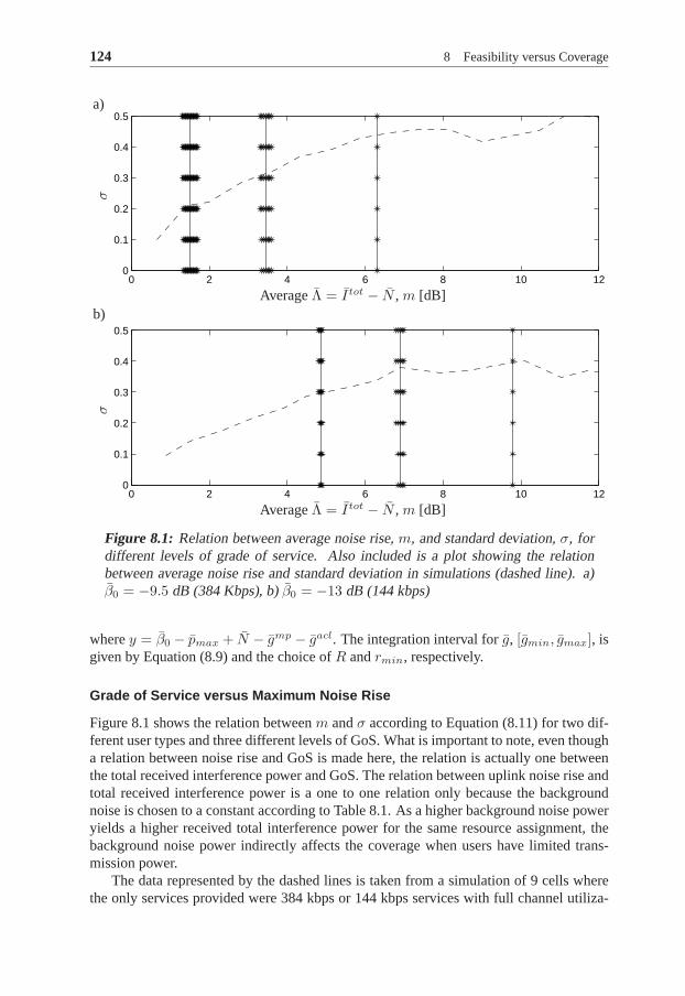
124 8 Feasibility versus Coverage
0 2 4 6 8 10 120
0.1
0.2
0.3
0.4
0.5
0 2 4 6 8 10 120
0.1
0.2
0.3
0.4
0.5
AverageΛ = Itot − N , m [dB]
AverageΛ = Itot − N , m [dB]
σσ
a)
b)
Figure 8.1: Relation between average noise rise,m, and standard deviation,σ, fordifferent levels of grade of service. Also included is a plotshowing the relationbetween average noise rise and standard deviation in simulations (dashed line). a)β0 = −9.5 dB (384 Kbps), b)β0 = −13 dB (144 kbps)
wherey = β0 − pmax + N − gmp − gacl. The integration interval forg, [gmin, gmax], isgiven by Equation (8.9) and the choice ofR andrmin, respectively.
Grade of Service versus Maximum Noise Rise
Figure 8.1 shows the relation betweenm andσ according to Equation (8.11) for two dif-ferent user types and three different levels of GoS. What is important to note, even thougha relation between noise rise and GoS is made here, the relation is actually one betweenthe total received interference power and GoS. The relationbetween uplink noise rise andtotal received interference power is a one to one relation only because the backgroundnoise is chosen to a constant according to Table 8.1. As a higher background noise poweryields a higher received total interference power for the same resource assignment, thebackground noise power indirectly affects the coverage when users have limited trans-mission power.
The data represented by the dashed lines is taken from a simulation of 9 cells wherethe only services provided were 384 kbps or 144 kbps serviceswith full channel utiliza-

8.3 Maximum Load 125
tion. Even though data is from two single service scenarios,the noise rise behavior isapproximately the same in a multi service scenario. The simulation results are thus ap-plicable to a multi service scenario. The variations in noise rise are a result of imperfectpower control due to, among other things, measurement errors, transmission power con-trol errors, inter-cell interference variations and user movement. Since the lines in bothplots in Figure 8.1 are rather steep, the standard deviationdoes not have a considerableimpact on the capacity and coverage. A major reason for the independence between GoSand noise rise variance is that the shadow fading variance isconsiderably larger than thenoise rise variance, thus
√
σ2s + σ2 ≈ σs. As can also be seen in Figure 8.1, the standard
deviation during simulations is quite small and also seems to be fairly service indepen-dent. From Figure 8.1 one can conclude that in order to achieve a 95 percent probability ofproviding service to a user assigned a 384-kbps-service with β0 = −9.5 dB, the averagenoise rise should not be much more than 3 dB. For a 144-kbps-service with β0 = −13 dB,the corresponding noise rise figure is almost 7 dB.
The link budgets clearly indicate a trade off between GoS andacceptable noise riselevels for a fixed background noise power. If the background noise power is increased,the maximum noise rise must decrease to the same extent. Nevertheless, the analysisshows that it is important to have accurate knowledge of the current noise rise level, orequivalently the load level, in order to guarantee a minimumgrade of service. What is notas obvious from the link budgets, which considers one user ata time, is how the currentnoise rise level, which depends on the situation in the entire system, is established.
Load versus Coverage
The same link budget as previously used to determine a maximum noise rise level givena fixed cell radius, can also be used to determine the maximum radius as a function ofthe target noise rise relative load. It is simply a matter of looking at the cell radius as avariable instead of a parameter, and conversely with the average noise rise.
Figure 8.2 shows the result of such calculations when the target GoS is 95 %. A modelstating that the average noise rise in dB is a linear functionof the cell radius has been fittedto data. The figure shows that a large cell radius requires a low choice of maximum loadlevel. Especially for large cell radiuses, the maximum noise rise relative load decreasesfast.
The shaded areas correspond to systems that can be expected to be capacity limited,as opposed to coverage limited. These areas correspond to system deployments with cellradiuses so small that the feasibility relative load is likely to be the limiting load. Putanother way, the performance for all cell radiuses is limited by the minimum requirementon noise rise relative load and feasibility relative load. In the shaded areas, it is thefeasibility relative load that defines the performance limitation.
8.3 Maximum Load
Two different scenarios are studied in the two previous sections, with and without usertransmission power limitations. Relations between capacity, coverage and users’ servicequality is established in a few special cases. Combining thetwo studies yields that the

126 8 Feasibility versus Coverage
0 200 400 600 800 1000 1200 1400 1600 18000
0.2
0.4
0.6
0.8
1N
oise
Ris
eR
elat
ive
Load
Cell Radius [m]
β0 = −13β0 = −9.5Data
Figure 8.2: Relation between average noise rise relative load and cell radius. Asimple model has also been fitted to data. GoS=95 %. The shadedarea representssituations where the system is capacity limited, as opposedto coverage limited. Aβ0 of -9.5 dB approximately corresponds to a 384 kbps service and β0 = −13 to a144 kbps service.
trade off is apparent regardless of the transmission power limitation, but different in dif-ferent scenarios.
Essentially, the system is interference limited as long as no users reach their transmis-sion power limit. This is likely to be the case in for example adense system, with smallcells with overlap. In these system, it is the feasibility relative load that sets the referencevalue for the resource management algorithms in Figure 1.1.
A system with large cells is likely to instead be limited by the amount of receivedinterference power due to the low power gain for users far from a base station. Users withlow power gain to the power controlling base station become sensitive to high receivedinterference power. Therefore, the maximum load will in this case be in terms of noiserise relative load.
Combining the results yields that the maximum uplink load depends on the specificdeployment. As such, it is also possible to improve the sceneby for example changingthe size of some cells or applying titled antennas with lowerantenna gain in suitabledirections.
8.4 Summary
This chapter focused on how load is related to coverage and capacity in terms of users’signal qualities. The relation was studied both in presenceand absence of user transmis-sion power constraints.
Two examples were used to show that a multi cell system is in fact coverage limited,even if the users have unlimited transmission powers. The limitation is in terms of thesum of users’ relative power gain values. This means that a load controlling algorithmcan increase the coverage for some users at the expense of other users.
In the case when users have limited transmission power, linkbudgets were used to

8.4 Summary 127
establish an approximative relation between grade of service, i.e., the probability of auser having service, and maximum uplink noise rise in the presence of a certain chosenbackground noise power. It was shown that if the maximum noise rise is chosen too highthe grade of service is considerably decreased. The same link budget approach was alsoused to establish an approximative relation between noise rise relative load and cell radiusfor a certain grade of service. The cell radius also decreases rapidly with increasing loadwhen the system is operated at high load levels.
The chapter has thus studied the well known trade off betweenperformance measuressuch as system capacity, coverage and service to individualusers. The overall resultconcerns what this trade off looks like in different deployments, and that it is very muchapplicable also when users do not have shortage of transmission powers.

128 8 Feasibility versus Coverage

9Filtering and Estimating Uplink Load
This chapter contains two signal processing application. In the first application, advancedfiltering is applied to a readily available load measurementgiven by any of the expressionsin Chapter 5. A biased auto-regressive signal model has beendeveloped and used. Usingthe model together with a change detection technique results in a stable estimate whichquickly adapts to new load levels. The work presented in thisfirst part of the chapter wasfirst published in (Geijer Lundin et al., 2003b).
The second application is estimation of the background noise power. Things get com-plicated due to a bias in the measurements. This makes the relation between measure-ments of the total received interference power on the one hand and the bias and back-ground noise power on the other, nonlinear. It is therefore useful to apply nonlinearestimation.
9.1 Adaptive Filtering Theory
The filtering and estimation techniques used in later sections of this chapter are hereexplained. Kalman filtering is explained in Section 9.1.1. Kalman filtering was firstdeveloped for linear filtering. One way of extending it to nonlinear applications is tolinearize the nonlinear model around a working point. A straight forward way is to choosea fixed working point. This idea is presented in Section 9.1.2. Another idea is to linearizeabout the best estimate of the current state values. This idea is used in the ExtendedKalman Filter (EKF) which is explained in Section 9.1.3. Theperhaps most sound ideais to not linearize at all, but instead simulate the system model as is done by the particlefilters. When using particle filters, several possible state vector values are considered atthe same time. In a sense, the most probable ones, based on measurements of the systemmodel output, are kept and the rest are discarded. Section 9.1.4 discusses the particle filtermethod.
129

130 9 Filtering and Estimating Uplink Load
A complication with applying any type of filtering or estimation is the trade off be-tween tracking and noise suppression. This can be somewhat relaxed by studying theresiduals of the estimation process. This idea and an implementation of it, the CUSUMalgorithm, are explained in Section 9.1.5. A good basis for using Adaptive filtering inpractice is given by Gustafsson (2000).
Introduce the notationx(t|τ) for the estimate ofx(t) given measurements until timeτ .The notation is justified by the fact that at each time instantthere is a measurement update,where the new measurement is considered, and a time update, where the predictions areupdated.
9.1.1 Kalman Filtering
A basis for applying Kalman Filtering is a linear system model,
x(t + 1) = Ax(t) + Bvw(t) (9.1a)
y(t) = C(t)x(t) + e(t), (9.1b)
where
x(t) =
x1(t)x2(t)· · ·
xn(t)
is the state vector containing the internal states of the model. Equation (9.1a) describes theinternal dynamics of the model while (9.1b) explains how thestate vector and measure-ment errors relate to the measurements,y(t). Theprocess noise, w(t), and themeasure-ment noise, e(t), are assumed to be white Gaussian noise with zero mean. As such, theyare completely characterized by their covariancesQ = Ew(t)w(t)T andR = Ee(t)e(t)T ,respectively.
The aim is to estimate the state vectorx(t) in the above state space model such thatthe covariance of the state error,E(x(t) − x(t))(x(t) − x(t))T , is minimized given mea-surementsy(t). A natural way of updating the state estimate with a new measurementis
x(t|t) = x(t|t − 1) + K(t)ǫ(t),
whereǫ(t) = y(t) − C(t)x(t|t − 1) is called theresidualat timet. Out of all possibleways of choosingK(t), the Kalman filter (Kalman, 1960) choosesK(t) such that thetwo-norm ofx− x is minimized. This optimality holds if the noise vectorsw(t) ande(t)are Gaussian distributed, otherwise the Kalman filter is thebest possible linear filter. TheKalman gain,K(t), is chosen based on knowledge of the measurement covariance, R, theprocess noise covariance,Q, and an estimate of the covariance of the current estimationerror,P (t|τ) = E(x − x(t|τ))(x − x(t|τ))T . SinceP (t|t) is time-varying it, too, has tobe updated. When using the Kalman filter, the update ofP (t), K(t) andx(t|t) is doneaccording to Algorithm 9.1. The covariance matricesQ andR are design parameters ofthe filter. Filteringy(t), as opposed to predictingy(t+1), corresponds to studyingx(t|t),as opposed tox(t + 1|t).To summarize, the Kalman filter delivers an estimate of the state vectorx(t), an estimatedcovariance matrix for this estimate (indicating the accuracy of the estimate),P (t|t), anda residualǫ(t) at each time instantt.

9.1 Adaptive Filtering Theory 131
Algorithm 9.1 Kalman filter
Initialization:x(0| − 1), P (0| − 1) = P0
Measurement update:
x(t|t) = x(t|t − 1) + K(t)(y(t) − C(t)x(t)
)
P (t|t) = P (t|t − 1) − K(t)C(t)P (t|t − 1)
whereK(t) = P (t|t − 1)C(t)T
(C(t)P (t|t − 1)C(t)T + R
)−1
Time update:
x(t + 1|t) = Ax(t|t)P (t + 1|t) = AP (t|t)AT + BvQBT
v
9.1.2 Linearized Kalman Filtering
The Kalman filter assumes that the system model is linear, both in the dynamics and in therelation between state vector and measured quantity. If this is not the case, the nonlinearmodel can be approximated by a linear model. To linearize themodel, a working pointabout which the model will be linearized must be chosen. Denote the chosen workingpoint byx0.
Consider a system with linear dynamics, i.e., the time update of the model is linear.The nonlinearity of the model is in the measurement equation. Thus, the studied model isof the type
x(t + 1) = Ax(t) + Bvw(t)
y(t) = h(x(t), t) + e(t).(9.2)
In general, the dynamics of the model can be also be time-varying, i.e., the matricesA andBv can depend on the time indext. However, (9.2) suffices for our needs. Once again,the process noisew(t) is independent white noise with zero mean and covariance matrixQ, and each measurement noiseej(t), j = 1, 2, . . . , B is zero mean Gaussian distributedwith covarianceR.
Using a Taylor expansion about an assumed trajectoryx0(t), h(x(t), t) may be ap-proximated as
h(x(t), t) ≈ h(x0(t), t) + H(t) (x(t) − x0(t)) ,
whereH(t)
△
= ∇xh(x(t), t)|x=x0(t).
When using thelinearized Kalman filter(LKF), Algorithm 9.1 is used to estimate
x(t)△
= x(t) − x0(t).

132 9 Filtering and Estimating Uplink Load
9.1.3 Extended Kalman Filtering
Theextended Kalman filter(EKF) is another algorithm for estimating the internal statesof the nonlinear model (9.2). EKF was first derived by Smith etal. (1962) and later bySchmidt (1966). A nice presentation of the filter based on thetraditional Kalman filteris given by Kailath (1980). A system with dynamics and additive noise is studied in theabove references, but the presentation here is limited to nonlinearities in the measurementequation only. The basic idea used in the EKF, is to always usea model linearized aboutthe last estimate of the state variables. This simply means thatx0(t) in the presentationof the linearized Kalman filter will be chosen as
x0(t) = x(t|t − 1),
at timet.The Kalman filter requires a linear relation between the statesx(t) and the measure-
ments. Approximatingh(x(t), t) in (9.2) with a first order Taylor expansion around thetime-varyingx0(t) yields
h(x(t), t) ≈ h(x(t|t − 1), t) + H(t) (x(t) − x(t|t − 1)) ,
whereH(t) = ∇xh(x(t), t)|x=x(t|t−1).
Consider a new system that has
y(t)△
= y(t) − h(x(t|t − 1), t) + H(t)x(t|t − 1) = H(t)x(t) + e(t)
as measurement equation. This new system has a linear relation between the measurementy(t) and the state vectorx(t). Applying the Kalman filter to this new system yields theEKF applied to the original system in (9.2).
The measurement update of the EKF when applied to the model in(9.2) is
x(t|t)=x(t|t − 1) + K(t) (y(t) − H(t)x(t|t − 1))
=x(t|t − 1) + K(t)(y(t) − h(x(t|t − 1), t) +
0︷ ︸︸ ︷
H(t)x(t|t − 1) − H(t)x(t|t − 1))
=x(t|t − 1) + K(t)(y(t) − h(x(t|t − 1), t)
).
This and the remaining steps taken by the extended Kalman filter at each time instant aredescribed by Algorithm 9.2.
9.1.4 Particle Filtering
Estimation can be seen as using noisy measurements togetherwith prior knowledge tocalculate the most probable value of the state vector. Therefore, a Bayesian approach isnatural. In the Bayesian estimation formulation the time update and the measurementupdate are expressed asprobability density functions(pdf). The idea in particle filters isto use numerical integration to express how the density functions for the values in the state

9.1 Adaptive Filtering Theory 133
Algorithm 9.2 Extended Kalman Filter
Initialization:P (0) = P0 andx(0| − 1)
Measurement update:
x(t|t) = x(t|t − 1) + K(t)ǫ(t)
P (t|t) = P (t|t − 1) − K(t)H(t)P (t|t − 1)
where
K(t) = P (t|t − 1)HT (t)(H(t)P (t|t − 1)H(t)T + R
)−1
H(t) = ∇xh(x(t), t)|x=x(t|t−1)
ǫ(t) = y(t) − h(x(t|t − 1)
)
Time update:
x(t + 1|t) = Ax(t|t)P (t + 1|t) = AP (t|t)AT + BvQBT
v
vector change as time evolves and new measurements are made.These density functionsare then used to make an estimate of the values in the state vector. Because Monte Carlointegration is used, particle filters are rather computationally intensive.
The presentation here will only be on the implementation of the particle filter. Risticet al. (2004) gives a comprehensive presentation of Monte Carlo integration and how it isused in particle filters.
It is called particle filters because several realizations,particles, of the state vectorare simulated simultaneously. It is these particles that are meant to characterize the pdfof the elements in the state vector. Algorithm 9.3 specifies the particle filter. Almostarbitrarily density functions can be used to describe the measurement and process noise,not just Gaussian. However, the measurement noise must be additive. Another strengthof particle filter is that there is no need to linearize the measurement equation nor anynonlinear dynamics.
9.1.5 Change Detection
An always present problem with traditional estimation is the trade off between trackingand noise suppression. A way of getting around this problem is to study the residuals,ǫ(t),of a process estimating the state vector of a system model. Inthe model used here, theresiduals are expected to be zero mean Gaussian with variance R, i.e., ǫ(t) ∈ N (0, R).If the estimates ofe(t), ǫ(t), are not zero-mean Gaussian or have a variance which isconsiderably greater thanR, there is reason to believe there has been an abrupt change inone or several of the parameters.
In order to detect a bias in the residuals, the squared normalized residuals (normalized

134 9 Filtering and Estimating Uplink Load
Algorithm 9.3 Particle Filter
Initialization:
Initialize the particles,xi(0| − 1), such that they cover the true state vector.
Measurement update:
• Calculate residuals for each particlei:
ǫi(t) = y(t) − h(xi(t|t − 1), t), i = 1, 2, . . . , N.
• Calculate the probability for each residual,pi = Pe(ǫi) using the pdf of the mea-surement noise.
• Normalize the probabilities:pi = piPNi=1 pi
.
Resampling:
Sample particles with replacement according to the discrete probability dis-tribution given bypi, i = 1, 2, . . . , N .
Time update:xi(t + 1|t) = Axi(t|t) + wi(t), i = 1, 2, . . . , N
wherewi(t) is drawn from the process noise’s pdf.
with their estimated standard deviation),ǫ2, are fed to a distance measurement algorithm.At every time instant this algorithm adds the normalized residual minus a drift termνto the previous accumulated distance. Hence, several consecutive residuals with consid-erable large magnitude will result in a growing distanceg(t), and eventually a changedetection onceg(t) has exceeded a fix threshold,h. Thecumulative sum (CUSUM)algo-rithm (Gustafsson, 2000) is defined by Algorithm 9.4 which isrun through at each updateof the state vector estimate. Once a change is detected, the filter characteristics is some-
Algorithm 9.4 CUSUM
g(t) = g(t − 1) + ǫ(t)2 − νif g(t) < 0
g(t) = 0endif g(t) > h
g(t) = 0flag for detected change
end
how temporarily changed in order to quickly adapt to the new situation. Figure 9.1 showsthe different parts of the adaptive filter applied in this chapter and how the behaviour ofthe algorithms are decided by a number of design parameters.

9.2 Load Filtering 135
y(t) EstimationAlgorithm
Distance-measure Thresholding
Parameters of
the model CUSUM
hνR, Q
ǫ(t)
detected change
g(t)
Figure 9.1: The different parts and parameters of an adaptive filter withchangedetection.
9.2 Load Filtering
The approximations given in Chapter 5 produce results whichwill fluctuate over time. Asdiscussed in Section 9.2.1, the goal with the work in this section is primarily to provide amore stable approximation. In order to suppress the fluctuations, a signal model describ-ing the fluctuations as well as the load level which the approximations fluctuate about isdeveloped in Section 9.2.2. The filtering involves using Kalman filter and a CUSUM de-tector. The choice of parameter values for these algorithmsare discussed in Section 9.2.3.Finally, adaptive filtering is applied to the model in Section 9.2.4.
Outcomes of the uplink noise rise relative load approximations in Chapter 5 will in thischapter be considered as measurements fed to the filtering process. They will thereforebe referred to as measurements of the uplink load. They should not be mistaken for loadapproximations based on measurements of the uplink interference power.
9.2.1 Motivation
As can be seen in Figure 9.2, the raw measurement of the noise rise relative load has,just as the true load, a trend and low frequency oscillationson top of this trend. Theoscillations are due to the user movement; as the users move around in the environmenttheir number of soft handover links regularly changes. Figure 9.3 shows that oscillationsin a cell’s uplink noise rise are strongly correlated with oscillations in the number of softhandover links. These oscillations can easily be canceled by low pass filtering the signal.However, applying a simple low pass filter could be risky since it is important to be alerton sudden changes in the load. Therefore, a signal model together with Kalman filteringand change detection is applied to the noise rise relative load estimate in order to reducenoise and oscillations while keeping track of sudden changes in the signal. A more stablesignal enables operation at a higher load level since the resource management algorithmswould not need as large margin to secure stability of the system. The time-varying modelalso provides an indication of towards where the load is currently heading, somethingwhich enables more aggressive resource management algorithms, e.g., PID-control.

136 9 Filtering and Estimating Uplink Load
0 10 20 30 40 50 60 70 80 90 1000.5
0.55
0.6
0.65
0.7
Time, [s]
Noi
seris
ere
lativ
elo
ad
Figure 9.2: Low frequency oscillations in relative load. Solid: Low pass filtered truenoise rise relative load. Dashed: Approximative noise riserelative load according to(5.13c).
0 10 20 30 40 50 60 70 80 90 10016
17
18
19
20
21
22
23
Time, [s]
Figure 9.3: Oscillations in uplink noise rise are strongly correlated with the numberof soft handover links. Thick: scaled and low pass filtered noise rise, thin: numberof soft handover links

9.2 Load Filtering 137
9.2.2 Signal Model
When dealing with signals whose behaviour is expected to change, continuously orabruptly, a fixed model is obviously not attractive. Using a parameterized signal modeland estimating not only the actual signal value but also the parameters of the model en-ables a more accurate signal estimate as well as an earlier detection of an abrupt change,in the parameters and/or the signal level. A signaly(t), originating from an unbiasedn:thorder Auto Regressive (AR)-model, may be described as (Ljung, 1999)
y(t) + a1y(t − 1) + a2y(t − 2) + ... + any(t − n) = e(t), (9.3)
wheree is white Gaussian noise with zero mean anda1, a2, ..., an are the parameters ofthe model. The signaly(t) in (9.3) will haveEy(t) = 0, but the signals we study haveEy(t) = L(t), whereL(t) is a time-varying bias. Therefore, a slightly more complexmodel is used, in which the time-varying bias is subtracted from eachy(t) givingE(y(t)−L(t)) = 0. Replacingy(t) by y(t) − L(t) in (9.3) yields
(y(t) − L(t)) +
n∑
i=1
ai(y(t − i) − L(t − i)) = e(t). (9.4)
This equation defines what can be described as a biased AR model, the oscillations are nolonger restricted to be around zero. There are other alternatives when modeling a signalwith oscillations around a non zero mean. Alasti and Farvardin (2000) use non-zero-meanGaussian noise to derive an expression for a biased AR model which is used to model theamount of requested bandwidth in a wireless network. A fourth order biased AR modelis used to describey, i.e., n = 4 in (9.4). It is natural to assume different time scalesof the bias variation and the dynamics, otherwise the AR-model is ambiguous. That is,the AR-model takes care of short term oscillations andL(t) models the long term drifts.Equation (9.4) may, under these assumptions, be approximated with
y(t) = L(t)
(
1 +4∑
i=1
ai
)
−4∑
i=1
aiy(t − i) + e(t). (9.5)
A state space representation of (9.5) in discrete time is
x(t) =(
L(t) ˙L(t) a1 a2 a3 a4
)T
x(t + 1) =
1 T 00 1 00 0 E4
x(t) +
T 2
2 0T 00 T E4
w(t)
y(t) =(1 +
∑ai 0 −y(t − 1) · · · − y(t − 4)
)x + e(t),
wherew(t) is a 5-dimensional vector containing the process noise andE4 is the4×4 iden-tity matrix. Note that the measurementy(t) has a non-linear relation to the parameters.This makes the parameter estimation more difficult. By introducing two new variables,
L = (1 +∑
ai)L and ˙L, the nonlinear state space model is converted into a linear state

138 9 Filtering and Estimating Uplink Load
space model according to
x(t) =(
L(t) ˙L(t) a1 a2 a3 a4
)T
x(t + 1) =
1 T 00 1 00 0 E4
x(t) +
T 2
2 0T 00 T E4
w(t) (9.6)
y(t) =(1 0 −y(t − 1) · · · − y(t − 4)
)x(t) + e(t).
Even though ˙L(t) includes time derivatives ofai, the variation in the bias can perhapsbe assumed far larger in magnitude than the variations in theAR-parameters and thus˙L(t) ≈ (1+
∑ai)
˙L. Assume the parameters to be independent of each other. Thisresultsin a diagonal covariance matrix for the process noise,Q, with elementsq1, q2 · · · q5 in thediagonal. The valuesq2 to q5 are all the same and much less thanq1. Hence we encourage
changes inL and ˙L rather than in the AR-parameters. The innovations,e(t) are assumedto be zero mean Gaussian with constant varianceR.
The conversion fromL back toL is
ˆL(t) =ˆL(t)
1 +∑4
i=1ˆai(t)
=ˆx1(t)
1 +∑6
k=3ˆxk(t)
. (9.7)
Var ˆL(t) ≈ L′ˆx(t)
TCov ˆx(t)L′
ˆx(t).
The expression for the variance is motivated by studying a first order Taylor expansion ofˆL(t).
9.2.3 Design Choices
Figure 9.4 shows an example of a raw signal produced by the load estimation (i.e., (5.16c)and (4.3)). The period of the slowest oscillations is about 20 seconds. The sampling timeof this signal isTframe = 0.01 seconds. Thus the slowest oscillations have a period ofabout 2000 samples. To describe the correlation in a signal having oscillations with such along period would require thousands of parameters. A rule ofthumb is that the fundamen-tal period of the oscillations to be modeled should be approximately 10 samples (Ljung,1999). Therefore every two hundredth sample is used when constructing the regressionvector,C(t). This is a kind of down sampling which requires an anti alias filter to beapplied. The chosen low pass filter is a second order filter with both its poles on the realaxis,
y(t) =4 · 10−4
1 − 1.96q−1 + 0.9604q−2L(t).
This results in a filter which does not introduce any additional oscillations but on the otherhand does not have a linear phase shift. Since it is the low frequencies of the signal that arestudied here, a linear phase shift is not a requirement here.The choice of filter bandwidthis a trade off between low alias effects and small time delay between input and output ofthe anti-alias filter.

9.2 Load Filtering 139
1150 1200 1250 1300 1350 1400 14500.4
0.42
0.44
0.46
0.48
0.5
0.52
0.54
0.56
t[s]
Noi
seris
ere
lativ
elo
ad
Figure 9.4: Example of noise rise relative load as function of time.
The state space representation in (9.6) has to be slightly modified to adapt to theresampling. Thus the final state space model used in the simulations is
x(t) =(
L(t) ˙L(t) a1 a2 a3 a4
)T
x(t + 1) =
1 T 00 1 00 0 E4
x(t) +
T 2
2 0T 00 T E4
w (9.8)
y(t) =(1 0 −y(t − 200) · · · −y(t − 800)
)x(t) + e(t).
Note thaty(t) is the output from the anti-alias filter, andT is the update rate of the filtertimes the length of a frame,Tframe = 0.01 s. The Kalman filter is parameterized bythe constants in the matrixQ and the scalarR, which thus can be seen as filter designvariables. A larger value in one ofQ’s components means that the corresponding statevariable(s) are more willing to change during the time between two time instants, whereasa largerR corresponds to less measurement accuracy. Hence, largerQ results in largerK and largerR results in a filter which puts less trust in the measurements and K istherefore chosen smaller yielding a ”slow” filter. The choice ofQ versusR is thus a tradeoff between tracking and noise suppression. The design parameterR should be chosensuch that it approximately equals the variance of the residuals.
Another design choice concerns the update rate of the filter.A reason for not choosinga faster update rate, which of course provides a possibilityfor earlier detection of largechanges in the relative load, is the increased computational burden a higher update rateinduces. So perhaps updating every sample is not an obvious choice. We have studiedfilter that has an update rate of every tenth or every hundredth estimate sample. Simula-tions show that the performance in steady state when filtering is the same regardless ofthe update rate.
The behaviour of the CUSUM detector is primarily decided by the parametersh andν. These have been chosen in such a way that we detect sudden changes of considerableamplitude within a reasonable time without having too many false alarms. In an attempt to

140 9 Filtering and Estimating Uplink Load
make the detection time independent of the update rate of thefilter, h is chosen inverselyproportional to the time between updates, i.e.,
h =Tframe
Th0,
whereh0 is the threshold used when updating every frame. In case of a change detection,the values ofP corresponding tox1 andx2 are increased a factor five, which results inmaking filtered value of these states more sensitive to the current input to the filter,y(t).The motivation for increasing only these two states is that the change is believed to be inthe load level and not in the AR parameters.
9.2.4 Simulations
Input data for this estimation application is taken from simulations produced by the simu-lator explained in Appendix A.1. A Kalman filter is used to extract the load levelL fromthe signaly in (9.5). By using the change detection technique describedin Section 9.1 thefilter is able to follow any sudden jumps in the load estimate.
Figure 9.5a shows the approximation ofL in (4.3) whereΛ is approximated using(5.16c). Also shown in Figure 9.5a is the Kalman filter estimate. The filter estimate is up-dated every frame, soT = Tframe = 0.01 s. The filtered estimate is free of oscillationsand follows an underlying trend in the original estimate. Note how the filtered estimatejumps when there is a distinct jump in the raw estimate. Figure 9.5b shows a close upversion of the top plot together with a rough low pass filteredversion of the original esti-mate. Both filters suppress noise equally well, but the low pass filtered signal adapts to thenew load level much slower. In case of a sudden jump upwards, the slow acclimatizationof the low pass filtered signal can be risky. In case of a jump downwards, the resourceutilization can be improved compared to using the low pass filtered version.
As a comparison, Figure 9.5c shows the performance of the filter when using threedifferent update rates; once every frame as above, once every tenth frame and once everyhundred frame. In steady state, the three versions of the filtering provide almost identicaloutputs. But, due to its superior update rate, the version which is updated every framedetects the jump earlier. However, all three update rates adapt to the new load level farfaster than the simple low pass filtered signal, also shown Figure 9.5c. Thus, a fasterupdate rate is perhaps not crucial, especially when comparing with the low pass filteredversion. The estimation process also provides an estimate of the derivative of the trend inthe relative load which enables a more aggressive resource management.
Due to the anti alias filter applied before the Kalman filter, the measurement noisee(t) is no longer white. Therefore, the residuals from the estimation process are not whiteeither. This indeed indicates the need for a more complex model, for example an ARMAmodel. However, as the simulations show, the proposed filterstill manages to provide agood estimate of the underlying trend in the relative load estimate.
9.3 Background Noise Power Estimation
Section 7.5 establishes that using inaccurate informationabout the background noisepower leads to unwanted transfer of resources between base stations. This section is de-

9.3 Background Noise Power Estimation 141
1150 1200 1250 1300 1350 1400 14500.4
0.45
0.5
0.55
1250 1260 1270 1280 1290 1300 1310 1320 1330 1340 13500.4
0.45
0.5
1298 1299 1300 1301 1302 1303 1304 1305 1306
0.4
0.45
0.5
Time [s]
Ln
rL
nr
Ln
r
a)
b)
c)
Figure 9.5: Performance of the Kalman filtering and change detection when appliedto a signal with a rather big jump in it. The different plots are magnified versionsof the same simulation. Solid: original estimate. Solid, thick: updated each frame.Solid, ring: updated every tenth frame. Solid, plus: updated every hundredth frame.Dashed: low pass filtered.

142 9 Filtering and Estimating Uplink Load
voted to estimating the background noise power ratio,θ, as defined in (7.13). An accurateestimate of the background noise power can, for example, be used by the load approx-imations based on iterations in Chapter 5. If the backgroundnoise powers are known,there is no need to assume equal background noise power during the derivation of theapproximations.
Definition 6.6 introduces the system matrix. Properties of this matrix was repeatedlyexplored in Chapter 6. Here, the same framework is used to estimate the background noisepower using measurements of the uplink interference power.Assuming that interferencepower measurements are available does in no way interfere with the motivation for study-ing uplink load approximations not using these measurements, as is done in Chapter 5. Onthe contrary, knowledge of the background noise power can beused instead of assuminga noise-flat system when deriving some of the approximationsin Chapter 5. Furthermore,another reason for not using measurements of the uplink interference power for load ap-proximations is that individual measurements may be associated with considerable errors,something which the background noise power application is not as sensitive to.
Unfortunately, measurements of the total uplink interference power is often corruptedby a bias in logarithmic scale, which also needs to be estimated. The state vector is thus
x(t) =
(θ(t)δ(t)
)
, (9.9)
whereδ(t) ∈ RB is the vector with base station individual biases.
The biases and the background noise power are related to measurements of the totalinterference power in Section 9.3.1, where the relation is expressed as the measurementequation in a state space model. The state space model is derived under an assumptionof connectivity one but this requirement is relaxed via an approximation in Section 9.3.2.A basic requirement for possibility of estimating the values in the state vector, is that theconnection between them and measurements of the uplink interference power is strongenough, that they areobservable. Even though the individual states are not observable,products of bias and background noise power ratio in the different base stations are ob-servable, as is shown in Section 9.3.3. Fortunately, these are the products that will be usedin practice anyway. Section 9.3.3 also contains a discussion on how the base stations canuse these products together with measurements of the uplinkinterference power to esti-mate the current uplink noise rise. Finally, methods for nonlinear estimation are appliedin Section 9.3.4.
The basis for this estimation is the system of nonlinear equations in (5.6). These equa-tions lay the ground for the uplink load approximations in Chapter 5. Instead of solvingfor the uplink noise rise, as in Chapter 5, the equations are combined with measurementsof the uplink interference power in order to estimate the background noise power.
9.3.1 Connectivity One
The nonlinearities in (5.6) are due to soft handover. In caseof connectivity one, thesystem of nonlinear equations breaks down into a system of linear equations. It is shownin Section 6.1.2 that the system of equations then can be expressed in matrix form as
Itot(t) = C(t)N(t), C(t)△
= (E − L(t)T )−1 (9.10)

9.3 Background Noise Power Estimation 143
whereL(t) is the system matrix according to Definition 6.6. As opposed to the situationin Chapter 6, the time span studied here is too long for considering the users’ targetCTIR values and the relative power gain values as constant. In fact, it is crucial for thisapplication that there are variations over time, as will be discussed in Section 9.3.3.
Elementj of the functionh(x, t) describing the relation between the states and theinterference power measurement in base stationj is
hj(x(t), t)△
= 10 log10
(
N0δj(t)
B∑
k=1
Cj,k(t)θk(t)
)
= 10
(
log10(N0) + log10(δj) + log10
B∑
k=1
Cj,k(t)θk(t)
)
.
(9.11)
As the base station error factor,δj , j = 1, 2 . . . B, and the background noise ratio,θj , j = 1, 2 . . . B are modeled as integrated white noise, the system model becomes
(θ(t + 1)δ(t + 1)
)
=
(θ(t)δ(t)
)
+
(wθ(t)wδ(t)
)
y(t) = h(x(t), t) + e(t),
(9.12)
with x(t) given by (9.9).The expression for the element on rowj and columnk of H(t) used in the EKF
depends on whether it relates to an element inθ or δ.
Hj,k(t) =
∂hj(δ,θ)∂θk
|x=x(t|t−1) = 10log 10
Cj,k(t)PBk=1 Cj,k(t)θk(t|t−1)
if k ≤ B
∂hj(δ,θ)∂δk−B
|x=x(t|t−1) =
{10
log 101
δj(t|t−1), k = j + B
0, k 6= j + Bif k > B.
9.3.2 Higher Connectivity
In case of higher connectivity at least one mobile is power controlled by more than onebase station. In this case it is not as easy to express the relation between measured in-terference power and the model statesNj andδj . This is due to the lack of an explicitsolution to (5.6). As in Chapter 5, approximations can be applied to solve the systemof nonlinear equations. Both the linearized and EKFs require an explicit expression forh(x(t), t) in order to calculateH(t). Therefore, fix point iterations to solve the system ofnonlinear equations is not an option in this case.
A second way to solve the system of nonlinear equations is theone used in Sec-tion 5.2.2. This leads to an explicit, but approximative solution to the system of nonlinearequations. Basically, the denominator in the relative pathgain, zi,j , is substituted by asum of path gain values taken over the set of cells that the user is connected to. Thismeans that the element on rowk and columnj in the system matrix,L(t), in (9.10) issubstituted by
Lk,j(t)△
=∑
i∈ck
βtgti (t)
gi,j(t)∑
ℓ∈Kigi,ℓ(t)
.

144 9 Filtering and Estimating Uplink Load
Using the matrixL = [Lk,j ], the interference power can be approximated by an expres-sion similar to (9.11)
hj(x(t), t)△
= 10 log10
(
N0δj(t)
B∑
k=1
Cj,k(t)θk(t
)
,
whereC(t)△
= (E − L(t))−1.The particle filter can be applied with either of the methods discussed above, i.e., both
fix point iterations or using the sum of path gain values in thedenominator of relativepower gain values. However, no adapts of estimating the background noise power whenusing fix point iterations have been made in the simulations.
9.3.3 Estimation Limitations
A necessary condition for estimation isobservability. Loosely speaking, a system is ob-servable if the connection between outputs and internal states is strong enough to uniquelydetermine the value of the internal states given the outputs. In our model, (9.12), the in-ternal states are the2B variables found in the vectorsδ andN .
Definition 9.1 (Observability). An internal state (function of states) isobservableif,given measurements at time instants up untilt0, it is possible to establish what the state(function of states) is at timet0.
Merely by looking at the model, one can conclude that it is impossible to determinethe states uniquely since the biases,δj , always appear multiplied by a background noisepower ratioθk, e.g.,δ1θ1, δ1θ2 etc.
However, below it is shown that the products of biases and background noise powerratio are observable, i.e., that it is possible to estimate them based on measurementsyj(t).Specifically, it is products of typeδjθj that are of interest. If these products are known,it is possible to calculate the noise rise based on measurements of the uplink interferencepower,
Λj(t) =Ij(t)
N(t)=
yj(t)/δj(t)
θj(t)N0=
yj(t)
δj(t)θj(t)N0.
The products are observable if, given a number of measurements y(t), t = 1, 2, . . . , it ispossible to establish the value of the products uniquely. Itis much easier to show that theproducts are observable if the relation between them and a function of the measurementsis linear. The function obviously has to be one-to-one. Be choosing the function to
ylin = 10y/10,
the relation betweenylin and the products is linear. Applying the conversion to the mea-surements of the model (9.12) in a noise less scenario yields, at timet,
ylinj (t) =
B∑
k=1
Cj,k(t)δj(t)θk(t)N0, j = 1, 2 . . . , B.

9.3 Background Noise Power Estimation 145
Under the assumption thatδj andθj are approximately constant over a period of timet = t0, t0 + 1, . . . , t1, consider the following system of equations.
ylinj (t0) = N0
B∑
k=1
Cj,k(t0)δj(t0)θk(t0), j = 1, 2 . . . , B
ylinj (t0 + 1) = N0
B∑
k=1
Cj,k(t0 + 1)δj(t0)Nk(t0), j = 1, 2 . . . , B
...
ylinj (t1) = N0
B∑
k=1
Cj,k(t1)δj(t0)Nk(t0), j = 1, 2 . . . , B.
Skipping the time indices forδj andθj , these equations can be put in matrix form as
1
N0
ylin1 (t0)
ylin2 (t0)
...ylin
B−1(t0)ylin
B (t0)ylin1 (t0 + 1)
ylin2 (t0 + 1)
...ylin
B−1(t1)ylin
B (t1)
= O
δ1N1
δ1N2
...δ1NB
δ2N1
δ2N2
...δBNB
(9.13)
where
O △
=
C1(t0) 0 · · · · · · 00 C2(t0) 0 · · · 0...
. . ... .
. .....
.... . .
.. . CB−1(t0) 00 · · · · · · 0 CB(t0)
C1(t0 + 1) 0 · · · · · · 0
0. . .
.. . · · · 0...
. . ... .
. .....
.... . .
.. . CB−1(t1) 00 · · · · · · 0 CB(t1)
.
With Cj(t) being thej:th row ofC(t). Below are two different cases where the matrixOhas full rank.
• As the cross products in the right hand side of (9.13) are not of interest, it is sat-isfactory to be able to solve for products of typeδjθj . If, at time instantt′, C(t′)

146 9 Filtering and Estimating Uplink Load
is diagonal with all diagonal elements being nonzero, it is possible to estimate allδjθj from that time instant alone.
ylinj (t′) = Cj,j(t
′)δjθjN0, j = 1, 2, . . . , B.
• If C(t) is not diagonal, it is necessary to solve for products of typeδjθk as well.Equation (9.13) has a unique solution ifO has full rank. As there areB2 differentproducts in the vector in the right hand side, we need measurements from at leastBdifferent time instants. Furthermore, theC-matrix has to change over time in orderto generate different measurement equations (different rows) at different times,t =t0, t0 + 1, . . . , t2.
There are of course other cases where we can solve for the interesting products. Thesecond case above is however the case interesting in practice, since we in practice can beexpected to always have some active users in each cell. The main conclusion from thediscussion in this section is summarized in the Theoreom 9.1
Theorem 9.1 (Observability)If O achieves full rank within a time frame in whichδj(t) and Nj(t) may be assumedconstant for allj, it is possible to estimate all productsδjθj ∀j = 1, 2, . . . , B.
Proof: If O has full rank, it is possible to solve for all products in the vector in the righthand side of (9.13). Specifically, it is possible to determine δjθj , ∀j = 1, 2, . . . , B.
The requirement thatO must achieve full rank is met ifC(t) varies in a random fash-ion over time. This is the case if traffic is rapidly changing,e.g., due to fast scheduling.
9.3.4 Simulations
Once again, the simulator discussed in Appendix A.1 is used for producing simulationdata. This time realistic interference power measurementsare gathered together withinformation about the users’ target CTIR values and their path gain values to base stations.All values are averaged over a time frame of 100 millisecondsin the base stations beforebeing delivered to the central node where the actual estimation process takes place.
As the measurements are averaged over a relatively long timeperiod, compared toboth the fast variations in radio channel between users and base stations and the rapidvariations in users’ transmission rates, the measurementsdo not capture momentarily in-terference power peaks. Simulations indicate that it is still possible to accurately estimatethe products of the base station’s individual biases,δj , and their background noise powerratios,θj .
Table 9.1 and Table 9.2 show the statistics of 15 Monte Carlo simulations with 20000samples in each simulation. Theroot mean square error(RMSE) as defined by Gustafsson(2000) has been calculated as
RMSE =
1
MC
MC∑
ℓ=1
1
B
B∑
j=1
1
T
T∑
t=1
||θ(ℓ)j (t) − θℓ
j(t)||22
1/2
,

9.3 Background Noise Power Estimation 147
whereθℓj(t) is the true background noise power ratio in base stationj at timet in Monte
Carlo simulationℓ and[1, T ] is the interval over which statistics is studied. When calcu-lating the statistics in the table, the first 20 seconds of each simulation has been removed.
The two particle filters, PF1 and PF2, have 5000 and 10000 particles, respectively.The two filters provide roughly the same statistics, meaningthat there is either not muchto gain from adding even more particles, or the number of particles is far too small. Theextended Kalman filter actually provides slightly better performance in the case of con-nectivity one, which is the case that the model is designed for. The particles filters, how-ever, seems slightly more robust against the model error that connectivity three brings.Out of the proposed filters, all save for the linearized Kalman filter provides good estima-tion error statistics. Using an ordinary Kalman filter applied to a linearized model doesnot seem to work at all in this application. The true product of δj andθj is probably toofar from the chosen working point. The relatively poor performance of the particle filter,compared to the extended Kalman filter, may be explained by a property of particle filtersyielding that they perform worse when estimating parameters of a model with small pro-cess noise and many states (Gustafsson et al., 2002). The model contains 18 states andthe process noise is practically zero since bothθ andδ are assumed to be approximatelyconstant. Gustafsson et al. (2002) claims that it can be worth trying even more particlesin this case.
As the users’ path gain values are both averaged over quite a few time instants anddo not include the multi path fading, the model does not consider the TX increase. Fur-thermore, the TX increase is larger when using connectivityone compared to using con-nectivity three. This may explain some of estimation improvement when going fromconnectivity one to connectivity three. Another reason maybe the decreased intensity ofhigh interference power peaks when using connectivity three.
Table 9.1: Estimation errors when estimating the product of background noise ratioand the base station individual biases. PF1 and PF2 are particle filters with 5000 and10000 particles, respectively. Connectivity one. 15 MonteCarlo simulations.
Mean Var. RMSEEKF 0.05 0.04 0.21PF1 0.07 0.08 0.29PF2 0.07 0.09 0.30
Table 9.2: Estimation errors when estimating the product of background noise ratioand the base station individual biases. PF1 and PF2 are particle filters with 5000 and10000 particles, respectively. Connectivity three. 15 Monte Carlo simulations.
Mean Var. RMSEEKF −0.09 0.02 0.18PF1 −0.06 0.02 0.14PF2 −0.06 0.01 0.13
The statistics in Table 9.1 and Table 9.2 are calculated in linear domain. Correspond-

148 9 Filtering and Estimating Uplink Load
ing results for the case of connectivity three in logarithmic scale are given in Table 9.3.The table shows that the particle filters provide a smaller RMSE corresponding to a morereliable estimate. Furthermore, discussing the absolute numbers, an average error of0.4 dB and an error variance of0.6 means that the estimate is less than one dB wrongin approximately two thirds of the considered time instants. This is rather small consider-ing that the background noise takes values in a range of aboutthree dB and that there isa measurement bias on top of that. Figure 9.6 shows how the different estimates evolve
Table 9.3: Estimation statistics in logarithmic scale (dB) for connectivity three.
Mean Var. RMSEEKF −0.80 4.26 2.21PF1 -0.38 0.58 0.85PF2 -0.45 1.01 1.10
over time. Att = 20 s, the true background noise power jumps up with three dB andat t = 40 s it jumps back down again. The linearized Kalman filter is notshown in thepicture. The jump up corresponds to the true background noise ratio making a jump fromone to two. This jump corresponds to halveρ defined in Section 7.5. It is certainly notpossible to relate the jump in Figure 9.6 to a certain decrease in the estimated backgroundnoise ratio in for example Figure 7.6. Even so, it is still clear that if such a jump is notadapted to by a base station using a noise rise controlling algorithm, the base station’scapacity will decrease considerably. Figure 9.6 shows thatthe extended Kalman filter andthe two particle filters manage to adapt to the new backgroundnoise power level, despitethe sudden and substantial jump. Thus, if using the proposedtechnique for estimating thebackground noise power, it possible for a noise rise controlling algorithms to eventuallyoperate normally despite the sudden jump in the background noise level.
0 10 20 30 40 50 600.4
0.6
0.8
1
1.2
1.4
1.6
1.8
Time [s]
δθ
TrueEKF
PF2PF1
Figure 9.6: Estimation ofθδ. The true background noise power makes jumps att = 20 s andt = 40 s. The particle filters have 5000 (PF1) and 10000 (PF2) particles.The filters are initialized with a product equal to one. A system with connectivitythree has been simulated.

9.4 Summary 149
9.3.5 Implementation Aspects
When calculatingC(t), the system matrix,L(t), as in Definition 6.6 is used. The systemmatrix consists of ratios between users’ power gains. In practice, the central node isunlikely to receive information on the users’ instantaneous multi path fading. One way ofstill considering this fast changing part of the power gain is to compile the system matrixin the base stations.
Loosely speaking, the element on rowk and columnj of the system matrix representsthe load cellk causes in cellj. Since the base station receives frequent reports on thepower gains between users and several base stations, each base stationk can, on its own,calculate values representing an average of these load contributions,
Lk,j =1
T
T∑
τ=1
∑
i∈ck
gi,j(τ)
gi,k(τ)βtgt
i (τ).
Here,T is the number of time instants between each report from the base stations to thecentral node. Based on these reports, the central node wouldthen compile the systemmatrix and then use it to calculateC(t).
9.4 Summary
Due to user movement, the noise rise relative load is subjectto slow oscillations. Earlierwork has provided an approximation of the noise rise relative load which to a great extentcaptures these oscillations. In this chapter, a signal model which describes the noise riserelative load as a signal consisting of a bias with a trend together with a fourth order autoregressive model has been developed. A Kalman filter together with a change detectionalgorithm has been applied to the model. The result is a stable signal representing atime average of the uplink load. Unlike what an ordinary low pass filter would provide,the filter is still alert on sudden changes in the load level due to the change detectionalgorithm used. Furthermore, the filter provides an indication towards where the load isheading. This information enables more aggressive resource management, which in theend enables better resource utilization.
A straight forward way of controlling the uplink noise rise level is to measure theuplink interference power and divide it by a number representing the background noisepower. Two problems with this are that the interference power measurements are oftencorrupted by a bias in logarithmic scale and that the background noise power is unknown.The second application of this chapter is a way of centrally estimate the product of mea-surement bias and background noise power in the different base stations. This is done byusing advanced signal processing together with measurements of the interference powerand path gain between users and base stations. Simulations indicate that it is possible tosatisfactory estimate the product, despite the fact that both multi path fading and soft han-dover is considered in the simulations but not in the model used in the estimation process.Using this method, the base stations can calculate the uplink noise rise by measuring theuplink interference power and divide it by the estimated product. This gives, not onlysensitivity to variations in the background noise power, but also robustness to the interfer-ence power measurement bias. Better knowledge of the background noise power enables
150 9 Filtering and Estimating Uplink Load
better resource utilization as argued in Chapter 8. Furthermore, if the measurement biascan be eliminated, the need for it to be small is not as crucialfor good performance.

10Conclusions
Due to the nature ofcode division multiple access(CDMA), the uplink load of CDMAcellular radio system should be related to either received or transmitted interference power.In this thesis, load definitions based on both of these approaches are proposed and rela-tions between them explored. Intercell interference, i.e., interference received in or causedby users connected to another cell, is studied in all parts ofthe thesis.
A number of load approximations that explicitly consider the received intercell in-terference contribution to the uplink load are proposed. The approximations are inde-pendent of interference power measurements through the useof a model for the receivedinterference power together with users’ path gain reports.A time averaged load can beapproximated with negligible errors. However, the approximations use sparsely sampledinformation and can therefore not relate to momentarily load levels. A resource controlalgorithm based on the approximations can thus utilize the system’s soft capacity, but cannot adapt to fast variations in the radio environment.
A system matrix, describing the relation between users’ radio environment, back-ground noise power and the received interference power is developed and properties of itare repeatedly used. A first application is to establish a number of relations between thedifferent uplink load definitions. These include a load definition related to system feasibil-ity, i.e., whether there exists transmission power levels to support the resource demands.Relations between the load definitions and the load approximations are also derived. Thisanalysis yields that iterations involved in the load approximations converge to the trueuplink load under certain requirements on the true system.
It is generally acknowledged that the high control bandwidth required to adapt tofast variations in users’ radio environment can be achievedthrough decentralized control.Properties of the system matrix are used to design a number ofdecentralized resourceallocation algorithms. As these algorithms control the amount of transmittedintercellinterference, they are robust in the sense that system feasibility is guaranteed. Simula-tions indicate that the proposed algorithms provide equal performance as a completely
151

152 10 Conclusions
centralized algorithm with complete knowledge of all users’ radio environment.A straightforward way of controlling the uplink load is to measure the amount of
received interference power and divide by the background noise power. Yet another ap-plication of the system matrix is to estimate the backgroundnoise power based on mea-sured interference power. The resulting estimation errorsare negligible compared to theinterference power measurement errors.

AAppendix
A.1 Cellular Radio System Simulator
Properties of the simulator will be described in this section. First, algorithms and pa-rameters of the radio environment as well as user creation, movement and transmissionpatterns will be described. Later, properties of the systemsuch as base station and cellconfiguration are given together with resource management algorithms and parameters.
A wide range of algorithms and characteristics of a CDMA system is simulated, fromalgorithms operating at a short time scale such as power control and multi path fading tomechanisms/algorithms naturally operating on a far longertime scale such as user creationand link configuration. The simulator is an improved versionof the simulator included inZander et al. (2001).
A.1.1 Models
Attenuation. The simulator models the total power gain as a product of fourparts;antenna gain, distance attenuation, shadow fading and multi path fading. The three firstparts are considered fixed for a certain position in the simulator area throughout the entiresimulations. In the factor representing the antenna gain, adirection-dependent attenuationis modeled. The distance attenuation, or path loss, is parameterized through the path losscoefficient,α = 3.5 and the shadow fading throughd0 = 100 m andσ = 6 dB in themodels given in Section 3.1. Multi path fading is updated with a function of traveleddistance every simulation step. This is used to model the stochastics in the multi pathfading even for a given point in space. On top of this an extra component is used tomodel the performance of the link estimation algorithms of areal system. This factor isa function of the user’s speed. Characteristics of the multipath fading model is givenin (3GPP, 2000c) under the name of "3GPP Typical Urban". A rake receiver with threefingers is incorporated in the model.
153

154 A Appendix
User Movement and Transmission Behavior. The mobility model states that theusers move with a constant absolute velocity but with angular variations. There are twotypes of transmission behaviors. Both of them use full buffers, i.e., users always have datato send.
In the first one, admitted users are continuously transmitting between the time of ad-mission until their they have send all their data. The amountof data to send is randomlychosen from an exponential distribution. This is an exampleof slow radio resource man-agement(RRM).
Fast RRM is modeled in the second model, meaning that the users send only whenexplicitly told to do so. No specific amount of data is modeledin this case.
A.1.2 Other Features
Power Control The simulator updates the transmission power of all users atevery slot,i.e., at a rate of 1500 Hz. Feedback delay is implemented and power control errors aremodeled. The update rate is in agreement with what is done in WCDMA (3GPP, 2000b).
Radio Resource Management Session admission is performed every frame. Twodifferent frame lengths have been used in the simulations. Slow RRM corresponds to aframe length of 10 ms, and fast RRM corresponds to 2 ms. The shorter frame length isused in an enhanced version of the WCDMA uplink (Parkvall et al., 2005).
A.1.3 Simulator Utilization
Various parts of the simulator are used for different purposes. Table A.1 summarizes whatparts of the simulator that is used for different simulationpurposes.
Table A.1: Summary of where the different parts of the simulator are used.
PowerControl
PowerGainModeling
Mobility SlowRRM
FastRRM
Section 5.7 x x x xSection 7.1 x x x xSection 7.4 xSection 8.2.3 xSection 9.2.4 x x x xSection 9.3.4 x x x x
A.2 Positive Matrices Theory
The characterizing property of positive matrices is that they have only positive elements.The following theorem can be found in (Gantmacher, 1974, page 66). All inequalities inthis appendix should be interpreted component wise.

A.3 Schur Complement 155
Theorem A.1A non-negative matrixA always has a non-negative eigenvaluer such that the moduli ofall the eigenvalues ofA do no exceedr. To this ’maximal’ eigenvaluer there correspondsa non-negative eigenvector
Ay = ry, (y ≥ 0, y 6= 0).
The adjoint matrixB(λ) = (λE − A)−1∆(λ) satisfies the inequalities
B(λ) ≥ 0,d
dλB(λ) ≥ 0 for λ ≥ r.
Another word for moduli is absolute value and∆(λ) is the characteristic polynomialof A, ∆(λ) = |λE − A|.
Proof: See (Gantmacher, 1974).
Interesting consequences of the theorem related to this work are
• The maximum eigenvalue, i.e., the eigenvalue with largest absolute value, is realand positive
λ(A) = max eig(A) = max | eig(A)| ≥ 0
• The smallest real eigenvalue such that the inequality
Ay ≤ ry
has positive real solutionsy is the maximum eigenvalue.
• Choosingλ = 1 in the theorem yields that
(E − A)−1 =B(1)
∆(1)> 0
if the largest eigenvalue,r, is less than one andA is an irreducible matrix.
A strictly positive matrix is always irreducible.
A.3 Schur Complement
TheSchur Complementof a matrix is a useful tool for establishing whether a matrixispositive definite or not Zhou et al. (1995). Consider the matrix
X =
(A B
BT C
)
, (A.1)
whereA is a symmetric matrix. Assume that det(A) 6= 0 and define theSchur comple-mentof X as the matrix
S = C − BT A−1B.
By the construction ofS, it follows that1 X � 0 ⇒ S � 0 if A ≻ 0.

156 A Appendix
A.4 Proof of Theorem 6.5
Theorem 6.5 is repeated here for convenience.Theorem 6.5 (Bound on Uplink Feasibility Relative Load)Consider a noise-flat sys-
tem with connectivity one. The feasibility relative load,Lf is bounded below and aboveby
maxj
∑
ℓ∈cj
βtgtℓ ≤ Lf ≤ max
jLIMRC
j .
The two different inequalities will be proven in separate lemmas.
Lemma A.1In a system with connectivity one,
Lf ≤ maxj
LIMRCj ,
with equality in a single cell scenario.
Proof: In a system with connectivity one,LIMRCj can be expressed in vector form as
LIMRCj =
M∑
i=1
βtgti zi,j =
B∑
k1
∑
i∈ck
βitgtzi,j =
B∑
k=1
Lk,j .
The greatest approximation can then be expressed as
maxj
LIMRCj = ||L||1.
Theorem A.4 in Skogestad and Postlethwaite (1996) states that for any matrix norm
max | eig(L)| ≤ ||L||.According to Theorem 6.2,Lf = maxj | eig(L)| in case of connectivity one.In case of a single cell scenario, the matrixL =
∑
i βtgti , hence so thusLf which proves
that equality holds in a single cell scenario.
Lemma A.2In a system with connectivity one,
maxj
∑
ℓ∈cj
βtgtℓ ≤ Lf ,
with equality in and only in a single cell scenario.
Proof: The cases of single cell and multi cell are studied separately. The equality require-ment in case of a single cell system has already been handled the proof of Lemma A.1.Strict inequality is required in the multi cell case. The left hand side of the expression inthe lemma can be reformulated asmaxj Lj,j . As Lj,j is a principal minor ofL in caseof multi cell system,Lj,j is strictly less than the maximum eigenvalue ofL (Gantmacher,1974). This proves the strict inequality in the multi cell case and claim in the lemma isproved.
1The notationA ≺ B, whereA andB are matrices, means that the maximum eigenvalue ofA − B is lessthan 0.

A.5 Proof of Theorem 6.7 157
Proof: (Theorem 6.5)The theorem follows from Lemma A.1 and Lemma A.2.
A.5 Proof of Theorem 6.7
Consider the update function in Algorithm 6.1 in the case of connectivity one,
Λj(t, n) = 1 +M∑
i=1
βtgti (t) +
gi,j(t)∑
k∈Ki
gi,k(t)Λk(t,n−1)
=
1 +
M∑
i=1
βtgti (t)
gi,j(t)
gi,Ki
ΛKi= 1 +
M∑
i=1
βtgti (t)zi,jΛKi
.
As fixed point iterations are considered, the time index is dropped,t, for the target CTIRvalues,βtgt
i . Furthermore, the above expression for base stationj can be written for allbase stations in matrix form as
Λ(t, n) = 1 + ZT BKΛ(t, n − 1) = 1 + LT Λ(t, n − 1).
This linear recursion will converge, regardless of initialization point, if the eigenvalues ofL are all inside the unit circle. Finally, the system as the system is assumed feasible,
Lf < 1 ⇒ max eig(L) < 1.
The convergence point is found by inserting a constantΛ, independent of the indexn,into the above update formula.
Λ = 1 + LT Λ. (A.2)
This equation is the same as (6.3) in case of perfect power control and a noise-flat system.The convergence point of Algorithm 6.1 thus equals the true noise rise in a noise-flatsystem with perfect power control.
A.6 Proof of Theorem 6.8
A.6.1 Preliminaries
Introducef(x) as the update function of Algorithm 6.1,
fj(x)△
= 1 +
M∑
ℓ=1
βtgtℓ
gℓ,j∑B
k=1Kℓ,kgℓ,k
xk
, j = 1, 2 . . . , B. (A.3)
Lemma A.3
When Algorithm 6.1 is initialized with aΛ(t, 0) ≤ Λ and applied to a noise-flat feasiblesystem, the iterations are bounded above by the finite true noise rise vector,Λ.

158 A Appendix
Proof: (Lemma A.3)The theorem states that
f(Λ(t, 0)) ≤ Λ if Λ(t, 0) ≤ Λ.
Note that eachfj(x), j = 1, 2 . . . , B is a non-decreasing function inx. It is thus suffi-cient to show thatf(Λ) ≤ Λ. Introduce
pℓ(x)△
=βtgt
ℓ∑B
k=1Kℓ,kgℓ,k
xk
.
Next it is shown thatpℓ(x) is less than or equal to the true transmission power,pℓ.The actual power control algorithms are based on measurements of the the user’s
carrier-to-interference ratio(CIR), γℓ, instead of its CTIR. In case of maximum ratiocombining, the sum of the locally received CIR-values is studied. Because of the non-linear relation between CTIR and CIR,βtgt
ℓ = γtgtℓ /(1 + γtgt
ℓ ), a combined CIR equalto the target CIR does not imply that the combined CTIR equalsthe target CTIR, despiteperfect power control. The implication is true only in systems with connectivity one (i.e.,when the total received CTIR consist of just one received signal). In general the combinedCTIR is greater than or equal to the target CTIR,
∑
k∈Kℓ
βℓ,k =∑
k∈Kℓ
pℓgℓ,k
Ik=∑
k∈Kℓ
γℓ,k
1 + γℓ,k
≥∑
k∈Kℓ
γℓ,k
1 + γℓ=
γℓ
1 + γℓ= βℓ = βtgt
ℓ ,
whereβl,k andγl,k are the locally received CTIR and CIR, respectively. Solving for pℓ
above yields
pℓ ≥βtgt
ℓ∑B
k=1Kℓ,kgℓ,k
Ik
= pℓ(I) = pℓ(Λ)N.
Dividing the inequality by the common background noiseN and inserting it into (A.3)yield
fj(Λ) = 1 +
M∑
ℓ=1
pℓ(Λ)gℓ,j ≤ 1 +
M∑
ℓ=1
pℓ
Ngℓ,j = Λj .
Finally, all elements ofΛ are obviously finite since the system is feasible.
Lemma A.4The update function of Algorithm 6.1,f(x), is astandard interference functionas definedin Yates (1995).
See Section A.6.3 for an introduction to standard interference functions.
Proof: The statement follows by simply checking thatf(x) complies with the require-ments of a standard interference function,
• Positivity This property is obvious considering thatf(x) represents a noise riselevel.

A.6 Proof of Theorem 6.8 159
• Monotonicity Assumex′ ≥ x and study the denominator of an arbitrary userℓ’scontribution to the sum in (A.3),
B∑
k=1
Kℓ,kgℓ,k
x′k
≤B∑
k=1
Kℓ,kgℓ,k
xk.
Since the denominator of term in (A.3) is either unchanged ordecreased, user eachuserℓ’s contribution is either unchanged or increased. Thus,
fj(x′) = 1 +
M∑
ℓ=1
βtgtℓ
gℓ,j∑B
k=1Kℓ,kgℓ,k
x′
k
≥ 1 +
M∑
ℓ=1
βtgtℓ
gℓ,j∑B
k=1Kℓ,kgℓ,k
xk
= fj(x), j = 1, 2 . . . B.
• Scalability It suffices to consider one arbitrary component,fj(x), at a time. Forcomponentfj(x),
fj(µx) = 1 +∑
i
βtgti
gi,j∑B
k=1Kℓ,kgi,k
µxk
= 1 + µ∑
i
βtgti
gi,j∑B
k=1Kℓ,kgi,k
xk
< µ
(
1 +∑
i
βtgti
gi,j∑B
k=1Kℓ,kgi,k
xk
)
= µfj(x).
The inequality is true sinceµ is greater than one.
A.6.2 Proof of Theorem 6.8
Proof: (Theorem 6.8)The theorem claims that there is a solution,x, to the equationx = f(x) if the systemis feasible. According to Lemma A.3 the iterations in Algorithm 6.1 are bounded by thecompact, convex setC = {x ∈ R
B : 1 ≤ xj ≤ Λj}, if initialized with xj(0) = 1∀j andapplied to a noise-flat feasible system. Furthermore,f(x) is a continuous function onC.Therefore, according to Brouwer’s fixed point theorem (Ortega and Rheinboldt, 1970),there exists a vector,x0, such thatx0 = f(x0).
According to Lemma A.4, the existence of a solution to the equations and Theorem 2in Yates (1995) which is stated in Section A.6.3 below, the iterations in Algorithm 6.1will converge tox0.
A.6.3 Standard Interference Functions
Yates (1995) shows that, given the three conditions in the theorem below, the equilibriumpoint x∗ is unique in the entireRn. Furthermore, the convergence is independent of theinitialization point.

160 A Appendix
Theorem A.2 (Global Convergence)Assume that there exist ax∗ such thatf(x∗) = x∗ andf(x) satisfies the following prop-erties
• Positivity: f(x) > 0
• Monotonicity: Ifx ≥ x′ thenf(x) ≥ f(x′)
• Scalability: For allµ > 1, µf(x) > f(µx).
Then the iterationx(t + 1) = f(x(t)) converges tox∗ for all x(0) ∈ Rn.
The above inequalities should be interpreted component wise.
Proof: See Yates (1995).
A.7 Proof of Lemma 7.2
The schur complement discussed in Appendix A.3 will be used to prove the lemma. Com-paringX in (A.1) with the extended matrix in Lemma (7.5) yields
A = E, C = Ltgt2E andB = L.
Now, sinceA = E ≻ 0, the requirement in the lemma implies
Ltgt2E − LT L � 0 ⇔ LT L � Ltgt2E.
This means thatλk(LT L) ≤ Ltgt2, k = 1, 2, . . . B.
As the maximum eigenvalue of a matrix is less than or equal to its maximum singularvalue (Golub and van Loan, 1996, page 318) this gives
λ(L)△
= maxk
λk(L) ≤√
λ(LT L) ≤ Ltgt.
Bibliography
3GPP. Radio Resource Management. Technical Specification 3GPP TS 25.133, 3GPP,2000a.
3GPP. Physical radio procedures. Technical Specification 3GPP TS 25.214, 3GPP, 2000b.
3GPP. FDD Enhanced Uplink; Overall description. TechnicalSpecification 3GPP TS25.309, 3GPP, 2005.
3GPP. RRC Protocol Specification. Technical Specification 3GPP TS 25.331, 3GPP,1999.
3GPP. Physical radio procedures. Technical Specification 3GPP TR 25.943, 3GPP, 2000c.
Mehdi Alasti and Nariman Farvardin. A diffusion approximation for voice-data integra-tion in a wireless network. InProceedings of the IEEE Wireless Communications andNetworking Conference, Chicago, IL, USA, Sep 2000.
Sirikiat Ariyavisitakul and Li Fung Chang. Signal and interference statistics of a CDMAsystem with feedback power control.IEEE Transactions on Communications, 41(11),1993.
Fredrik Berggren and Riku Jäntti. Asymptotically fair scheduling on fading channels. InProceedings of the IEEE Vehicular Technology Conference, 2002.
Patrick Billingsley.Probability and Measure. John Wiley & Sons, LTD, 1995.
Peter J. Black and Qiang Wu. Link budget of cdma2000 1xEV-DO wireless internetaccess system. InProceedings of the IEEE Personal, Indoor and Mobile Radio Com-munications Conference, September 2002.
161

162 Bibliography
Hatem Boujemaa, Mohammed Siala, and Raphael Visoz. Multipath diversity and powercontrol. InProceedings of the IEEE Vehicular Technology Conference, Birmingham,Alabama, USA, May 2002.
Stephen Boyd and Lieven Vandenberghe.Convex Optimization. Cambridge UniversityPress, The Edinburgh Building, Cambridge, CB2 2RU, UK, 2004.
Pete Boyer, Milica Stojanovic, and John Proakis. A simple generalization of the CDMAreverse link pole capacity formula.IEEE Transactions on Communications, pages1719–1722, October 2001.
Jin-Ghoo Choi and Saewoong Bahk. Multiclass call admissioncontrol in QoS-sensitiveCDMA networks. InProceedings of the IEEE International Conference on Communi-cations, Helsinki, Finland, June 2001.
Jelena Damnjanovic, Avinash Jain, Tao Chen, and Sandip Sarkar. Scheduling thecdma2000 reverse link. InProceedings of the IEEE Vehicular Technology Conference,September 2002.
John Dennis Jr. and Robert B. Schnabel.Numerical Methods for Unconstrained Opti-mization and Nonlinear Equations. Prentice Hall, Englewood Cliffs, N.J., USA, 1983.
Nikos Dimitriou, Georgios Sfikas, and Rahim Tafazolli. Calladmission policies forUMTS. In Proceedings of the IEEE Vehicular Technology Conference, Tokyo, Japan,May 2000.
Xiang Duan, Zhisheng Niu, David Huang, and Dadvid Lee. A dynamic power and ratejoint allocation algorithm for mobile multimedia DS-CDMA networks based on utiliityfunctions. InProceedings of the IEEE Personal, Indoor and Mobile Radio Communi-cations Conference, September 2002.
Nan Feng, Siun-Chuon Mau, and Narayan B. Mandayam. Pricing and power control forjoint network-centric and user-centric radio resource management.IEEE Transactionson Communications, 52(9), 2004.
Felix R. Gantmacher.The Theory of Matrices, Vol. II, Ch. XIII. Chelsea PublishingCompany, New York, NY, USA, 1974.
Erik Geijer Lundin and Fredrik Gunnarsson. Uplink load in CDMA cellular radio sys-tems.IEEE Transactions on Vehicular Technology, 2005. To Appear.
Erik Geijer Lundin and Fredrik Gunnarsson. Characterizinguplink load - concepts andalgorithms. In Mohsen Guizani, editor,Wireless Communications Systems and Net-works, chapter 14, pages 425–441. Kluwer Academic, 2003.
Erik Geijer Lundin and Fredrik Gunnarsson. Using uplink relative path gain relatedmeasurements to support uplink resource management. US Patent Application No:11/066,558.
Erik Geijer Lundin, Fredrik Gunnarsson, and Fredrik Gustafsson. Uplink load estimatesin WCDMA with different availability of measurements. InProceedings of the IEEEVehicular Technology Conference, Cheju, South Korea, April 2003a.

Bibliography 163
Erik Geijer Lundin, Fredrik Gunnarsson, and Fredrik Gustafsson. Adaptive filtering ap-plied to an uplink load estimate in WCDMA. InProceedings of the IEEE VehicularTechnology Conference, Cheju, South Korea, April 2003b.
Erik Geijer Lundin, Fredrik Gunnarsson, and Fredrik Gustafsson. Uplink load estimationin WCDMA. In Proceedings of the IEEE Wireless Communications and NetworkingConference, New Orleans, LA, USA, March 2003c.
Erik Geijer Lundin, Fredrik Gunnarsson, and Fredrik Gustafsson. Robust uplink resourceallocation in CDMA cellular radio systems. InProceedings of the IEEE Conference onDecision and Control, Seville, Spain, December 2005a. To appear.
Erik Geijer Lundin, Fredrik Gunnarsson, and Fredrik Gustafsson. Uplink load andlink budget with stochastic noise rise levels in CDMA cellular systems. InRVK05,Linköping, Sweden, June 2005b.
Klein S. Gilhousen, Irwin M. Jacobs, Roberto Padovani, Andrew J. Viterbi, Lindsay A.Weaver Jr., and Charles E. Wheatley. On the capacity of a cellular CDMA system.IEEE Transactions on Vehicular Technology, 40(2), 1991.
Gene H. Golub and Charles F. van Loan.Matrix Computations. The Johns HopkinsUniversity Press, Baltimore, MD, USA, third edition, 1996.
Mikael Gudmundson. Correlation model for shadow fading in mobile radio systems.IEEElectronics Letters, 27(23), November 1991.
Fredrik Gunnarsson.Power Control in Cellular Radio System: Analysis, Design and Esti-mation. PhD thesis, Linköping University, Linköping, Sweden, April 2000. LinköpingStudies in Science and Technology. Dissertations No. 579.
Fredrik Gunnarsson, Erik Geijer Lundin, Gunnar Bark, and Niclas Wiberg. Uplink ad-mission control in WCDMA based on relative load estimates. InIEEE InternationalConference on Communications, New York, NY, USA, April 2002.
Fredrik Gunnarsson, David Törnqvist, Erik Geijer Lundin, Gunnar Bark, Niclas Wiberg,and Eva Englund. Uplink transmission timing in WCDMA. InIEEE Vehicular Tech-nology Conference, Orlando, FL, USA, October 2003.
Fredrik Gustafsson.Adaptive filtering and change detection. John Wiley & Sons, LTD,2000.
Fredrik Gustafsson, Fredrik Gunnarsson, Niclas Bergman, Urban Forssel, Jonas Jansson,Rickard Karlsson, and Per-Johan Nordlund. Particle filtersfor positioning, navigationand tracking.IEEE Transactions on Signal Processing, 50(2), February 2002.
Hwang Gyung-Ho and Cho Dong-Ho. Dynamic rate control based on interference andtransmission power in 3GPP WCDMA system. InProceedings of the IEEE VehicularTechnology Conference, Boston, MA, USA, September 2000.
Stephen Vaughan Hanly. Capacity and power control in spreadspectrum macrodiversityradio networks.IEEE Transactions on Communications, 44(2), 1996.

164 Bibliography
Stephen Vaughan Hanly and David N. C. Tse. Power control and capacity of spreadspectrum wireless networks.Automatica, 35:1987–2012, 1999.
Bassam Hashem and Elvino Sousa. Reverse link capacity and interference statistics ofa fixed-step power-controlled DS/CDMA system under slow multipath fading. IEEETransactions on Communications, pages 1905–1912, December 1999.
Bassam Hashem and Elvino Sousa. A combined power/rate control scheme for data trans-mission over a DS/CDMA system. InProceedings of the IEEE Vehicular TechnologyConference, pages 1096–1100, Ottawa, Ontario, Canada, May 1998.
Masayasu Hata. Empirical formula for propagation loss in land mobile radio services.IEEE Transactions on Vehicular Technology, 29(3), 1980.
Jeffrey D. Herdtner and Edwin K.P. Chong. Analysis of a classof distributed asyn-chronous power control algorithms for cellular wireless systems. IEEE Journal onSelected Areas in Communications, 18(3), March 2000.
Kimmo Hiltunen and Nicola Binucci. WCDMA downlink coverage:interference marginfor users located at the cell coverage border. InProceedings of the IEEE VehicularTechnology Conference, Birmingham, AL, USA, May 2002.
Harri Holma and Janne Laakso. Uplink admission control and soft capacity with MUD inCDMA. In Proceedings of the IEEE Vehicular Technology Conference, Amsterdam,the Netherlands, Sep 1999.
Harri Holma and Antti Toskala.WCDMA for UMTS, Radio Access For Third GenerationMobile Communications. John Wiley & Sons, LTD, 2000.
Ching-Yao Huang and Roy D. Yates. Call admission in power controlled CDMA systems.In Proceedings of the IEEE Vehicular Technology Conference, Atlanta, GA, USA, May1996.
Yoshihiro Ishikawa and Narumi Umeda. Capacity design and performance of call admis-sion control in cellular CDMA systems.IEEE Journal on Selected Areas in Communi-cations, 15(8), October 1997.
Ahmad Jalali. On cell breathing in CDMA networks. InProceedings of the IEEE Inter-national Conference on Communications, Atlanta, GA , USA, June 1998.
Riku Jäntti and Seong-Lyun Kim. Transmission rate scheduling for the non-real-time datain a cellular CDMA system.IEEE Communications Letters, 5(5), May 2001.
Tara Javidi. Decentralized rate assignments in a multi-sector CDMA network. InPro-ceedings of the IEEE Global Telecommunications Conference, Dec 2003.
Thomas Kailath.Linear Systems. Prentice Hall, Englewood Cliffs, NJ, USA, 1980.
Rudolph E. Kalman. A new approach to linear filtering and prediction problems.Journalof Basic Engineering, Transactions of the ASME, 82D:35–45, March 1960.

Bibliography 165
Joon Bae Kim and Michael L. Honig. Resource allocation for multiple classes of DS-CDMA traffic. IEEE Transactions on Vehicular Technology, 49(2):506–519, May2000.
Sang Wu Kim and Ye Hoon Lee. Combined rate and power adaptation in DS/CDMAcommunications over nakagami fading channels.IEEE Transactions on Communica-tions, 48(1), January 2000.
Raymond Knopp and Pierre A. Humblet. Information capacity and power control insingle-cell multiuser communications. InProceedings of the IEEE International Con-ference on Communications, Seattle, USA, June 1995.
Troels E. Kolding, Frank Frederiksen, and Preben E. Mogensen. Performance aspects ofWCDMA systems with high speed downlink packet access (HSDPA). In Proceedingsof the IEEE Vehicular Technology Conference, Vancouver, Canada, 2002.
Joy Kuri and Paul Mermelstein. Call admission on the uplink of a CDMA system basedon total received power. InProceedings of the IEEE International Conference on Com-munications, Vancouver, BC, Canada, June 1999.
Janne Laakso, Riku Jäntti, Mika Rinne, and Oscar Salonaho. Radio resource knapsackpacking for WCDMA air interface. InProceedings of the IEEE Personal, Indoor andMobile Radio Communications Conference, Boston, MA, USA, Sep 1998.
Jaana Laiho, Achim Wacker, and Tomás Novosad.Radio Network Planning and Optimi-sation for UMTS. John Wiley & Sons, LTD, 2002.
Zhuyu Lei, David J. Goodman, and Narayan B. Mandayam. Location-dependent other-cell interference and its effect on the uplink capacity of a cellular CDMA system. InProceedings of the IEEE Vehicular Technology Conference, Houston, TX, USA, May1999.
Xin Liu, Edwin K. P. Chong, and Ness B. Shroff. Opportunistictransmission schedulingwith resource-sharing constraints in wireless networks.IEEE Journal on Selected Areasin Communications, 19(10), October 2001.
Lennart Ljung. System Identification – Theory for the User. Prentice Hall, EnglewoodCliffs, NJ, USA., second edition, 1999.
Johan Löfberg. YALMIP : A toolbox for modeling and optimization in MATLAB.In Proceedings of the CACSD Conference, Taipei, Taiwan, 2004. Available fromhttp://control.ee.ethz.ch/˜joloef/yalmip.php .
Rohit Nagi, Moses Charikar, and John Cioffi. Minimum outage transmission over fadingchannels with delayconstraint. InProceedings of the IEEE International Conference onCommunications, pages 282–286, New Orleans, LA, USA, June 2000.
Thomas Neubauer and Ernst Bonek. Impact of the variation in the background noisefloor on UMTS system capacity. InProceedings of the IEEE Vehicular TechnologyConference, volume 4, pages 2435–2439, Rhodes, Greece, May 2001.

166 Bibliography
Seong-Jun Oh and Kimberly M. Wasserman. Optimal resource allocation in multiserviceCDMA networks.IEEE Transactions on Wireless Communications, 2(4), July 2003.
Yoshihisa Okumura, E Ohmori, T. Kawano, and K. Fukuda. Fieldstrength and its vari-ability in VHF and UHF land-mobile radio service.Review of the Electrical Commu-nication Laboratory, 16(9-10), 1968.
James M. Ortega and Werner C. Rheinboldt.Iterative Solution of Nonlinear Equations inSeveral Variables. Academic Press, London, 1970.
José Outes, Lars Nielsen, Klaus Pedersen, and Preben Mogensen. Multi-cell admissioncontrol for UMTS. InProceedings of the IEEE Vehicular Technology Conference,Rhodes, Greece, May 2001.
Roberto Padovani, B. Butler, and R. Boesel. CDMA digital cellular: field test results. InProceedings of the IEEE Vehicular Technology Conference, Stockholm, Sweden, June1994.
Stefan Parkvall, Janne Peisa, Johan Torsner, and Peter Malm. WCDMA enhanced uplink- principles and basic operation. InProceedings of the IEEE Vehicular TechnologyConference, Stockholm, Sweden, May 2005.
Ramin Rezaiifar and Jack Holtzman. Proof of convergence forthe distributed optimal rateassignment algorithm. InProceedings of the IEEE Vehicular Technology Conference,Houston, TX, USA, May 1999.
Branko Ristic, Sanjeev Arulampalam, and Neil Gordon.Beyond the Kalman Filter: Par-ticle Filters for Tracking Applications. Artech House, 2004.
Virgilo Rodriguez, David J. Goodman, and Marantz Zory. Power and data rate assignmentfor maximal weighted throughput in 3G CDMA: a global solution with two classes ofusers. InProceedings of the IEEE Wireless Communications and Networking Confer-ence, March 2004.
Ashwin Sampath, Kumar P. Sarath, and Jack M. Holtzmann. Power control and resourcemanagement for a multimedia CDMA wireless system. InProceedings of the IEEEPersonal, Indoor and Mobile Radio Communications Conference, Toronto, Ontario,Canada, September 1995.
Juan Sanchez, Jordi Pérez-Romero, Oriol Sallent, and RamónAgusti. Mixing conversa-tional and interactive traffic in the UMTS radio access network. In Proc.IEEE 4th In-ternational Workshop on Mobile and Wireless Communications Network, 2002, Stock-holm, Sweden, September 2002.
Stanley F. Schmidt. Application of state-space methods to navigation problems.Advancesin Control Systems, C.T. Leondes, Ed., Academic Press, 3:293–340, 1966.
Stuart C. Schwartz and Yu-Shuan Yeh. On the distribution function and moments ofpower sums with log-normal components.The Bell System Technical Journal, 61(7),1982.

Bibliography 167
Kari Sipilä, Jaana Laiho-Steffens, Achim Wacker, and Mika Jäsberg. Modeling the impactof the fast power control on the WCDMA uplink. InProceedings of the IEEE VehicularTechnology Conference, Houston, Texas, May 1999.
Bernard Sklar. Rayleigh fading channels in mobile digital communication systems.IEEECommunications Magazine, 35(7), 1997.
Sigurd Skogestad and Ian Postlethwaite.Multivariable Feedback Control. John Wiley &Sons, LTD, 1996.
Gerald L. Smith, Stanley F. Schmidt, and Leonard A. McGee. Application of statisticalfilter theory to the optimal estimation of position and velocity on board a circumlunarvechicle. Technical report, NASA TR T-35, National Aeronautics and Space Adminis-tration, 1962.
Peter Stevens. Operator design and planning issues for UMTSnetworks. InIEE Collo-quium on UMTS - The R&D Challenges (Ref. No. 1998/496), London, UK, November1998.
Bogdan Timus and Jonas Pettersson. Uplink admission control for conversational servicesusing information from many cells. InProceedings of the IEEE Vehicular TechnologyConference, Rhodes, Greece, May 2001.
Kim C. Toh, Michael J. Todd, and Reha H. Tütüncü.SDPT3 — a MATLAB softwarepackage for semidefinite programming, version 3.02, September 2001.
David Törnqvist, Erik Geijer Lundin, Fredrik Gunnarsson, and Fredrik Gustafsson. Trans-mission timing - a control approach to distributed uplink scheduling in WCDMA. InProceedings of the American Control Conference, Boston, MA, USA, June 2004.
Sennur Ulukus and Larry J. Greenstein. Throughput maximization in CDMA uplinksusing adaptive spreading and power control. InProceedings of the Symposium onSpread Spectrum Techniques and Applicatoins, September 2000.
John M. Wozencraft and Irwin Mark Jacobs.Principles of Communication Engineering.John Wiley & Sons, LTD, 1965.
Roy D. Yates. A framework for uplink power control in cellular radio systems.IEEEJournal on Selected Areas in Communications, 13(7), September 1995.
Wang Ying, Zhang Jingmei, Wang Weidong, and Zhang Ping. Calladmission control inhierarchi cell structure. InProceedings of the IEEE Vehicular Technology Conference,Birmingham, AL, USA, May 2002.
Jens Zander. Transmitter power control for co-channel interference management in cel-lular radio systems. InProc. WINLAB Workshop, New Brunswick, NJ, USA, October1993.
Jens Zander, Seong-Lyun Kim, Magnus Almgren, and Olav Queseth. Arthech House,2001.

168 Bibliography
Qinqing Zhang and On-Ching Yue. UMTS air interface voice/data capacity - part 1:re-verse link analysis. InProceedings of the IEEE Vehicular Technology Conference,Rhodes, Greece, May 2001.
Kemin Zhou, John C. Doyle, and Keith Glover.Robust and Optimal Control. PrenticeHall, Upper Saddle River, NJ, USA, 1995.

Index
3GPP, 37
active set, 32admission control, 35
background noise power ratio, 114base station, 30
capacity, 33capacity limited system, 121carrier-to-total-interference ratio, 31CDMA, 29cell, 30cellular radio network, 30channel switching, 36chip rate, 29CIR, 28, 31congestion control, 36connectivity, 82
strict, 82correlation distance, 26coverage limited system, 121CTIR, 31CUSUM, 134
downlink, 30
enhanced uplink, 38
fast fading, 27FDMA, 29feasibility, 82feasibility relative load, 85
grade of service (GoS), 33
handover, 31soft, 32softer, 38
hard capacity, 42
intercell-to-intracell-interference factor, 44interference
intercell, 33, 43intracell, 43total, 31
interference limited system, 41
Kalman filterextended, 133linear, 131
link admission, 36link matrix, 82
maximum ratio combining, 32multipath fading, 27
169

170 Index
noise limited system, 41noise rise, 40noise rise relative load, 41non-orthogonal signals, 29
observability, 144orthogonal signals, 29
packet scheduling, 36particle filter, 134party effect, 35path loss, 26pole capacity, 41power control, 31, 34power gain, 26power gain matrix, 30processing gain, 29propagation exponent, 26
Quality of Service (QoS), 33
radio network controller (RNC), 37radio resource management (RRM), 34rake, 27relative power gain matrix, 83RRM, 34
selection combining, 32self interference factor, 32shadow fading, 26SIR, 28soft capacity, 42soft resource, 43spreading code, 29system feasibility, 82system matrix, 83system noise rise relative load, 84
TDMA, 29total interference power, 31TX increase, 64
uplink, 30
WCDMA, 37
PhD DissertationsDivision of Automatic Control
Linköpings universitet
M. Millnert: Identification and control of systems subject to abrupt changes. Thesis No. 82, 1982.ISBN 91-7372-542-0.A. J. M. van Overbeek: On-line structure selection for the identification of multivariable systems.Thesis No. 86, 1982. ISBN 91-7372-586-2.B. Bengtsson:On some control problems for queues. Thesis No. 87, 1982. ISBN 91-7372-593-5.S. Ljung: Fast algorithms for integral equations and least squares identification problems. ThesisNo. 93, 1983. ISBN 91-7372-641-9.H. Jonson: A Newton method for solving non-linear optimal control problems with general con-straints. Thesis No. 104, 1983. ISBN 91-7372-718-0.E. Trulsson: Adaptive control based on explicit criterion minimization. Thesis No. 106,1983.ISBN 91-7372-728-8.K. Nordström: Uncertainty, robustness and sensitivity reduction in the design of single input con-trol systems. Thesis No. 162, 1987. ISBN 91-7870-170-8.B. Wahlberg: On the identification and approximation of linear systems. Thesis No. 163, 1987.ISBN 91-7870-175-9.S. Gunnarsson:Frequency domain aspects of modeling and control in adaptive systems. ThesisNo. 194, 1988. ISBN 91-7870-380-8.A. Isaksson: On system identification in one and two dimensions with signal processing applica-tions. Thesis No. 196, 1988. ISBN 91-7870-383-2.M. Viberg: Subspace fitting concepts in sensor array processing. Thesis No. 217, 1989. ISBN 91-7870-529-0.K. Forsman: Constructive commutative algebra in nonlinear control theory. Thesis No. 261, 1991.ISBN 91-7870-827-3.F. Gustafsson: Estimation of discrete parameters in linear systems. Thesis No. 271, 1992.ISBN 91-7870-876-1.P. Nagy: Tools for knowledge-based signal processing with applications to systemidentification.Thesis No. 280, 1992. ISBN 91-7870-962-8.T. Svensson:Mathematical tools and software for analysis and design of nonlinear control systems.Thesis No. 285, 1992. ISBN 91-7870-989-X.S. Andersson:On dimension reduction in sensor array signal processing. Thesis No.290, 1992.ISBN 91-7871-015-4.H. Hjalmarsson: Aspects on incomplete modeling in system identification. Thesis No. 298, 1993.ISBN 91-7871-070-7.I. Klein: Automatic synthesis of sequential control schemes. Thesis No. 305, 1993. ISBN 91-7871-090-1.J.-E. Strömberg: A mode switching modelling philosophy. Thesis No. 353, 1994. ISBN 91-7871-430-3.K. Wang Chen: Transformation and symbolic calculations in filtering and control. Thesis No. 361,1994. ISBN 91-7871-467-2.T. McKelvey: Identification of state-space models from time and frequency data. Thesis No. 380,1995. ISBN 91-7871-531-8.J. Sjöberg: Non-linear system identification with neural networks. Thesis No. 381, 1995. ISBN 91-7871-534-2.R. Germundsson: Symbolic systems – theory, computation and applications. Thesis No. 389,1995. ISBN 91-7871-578-4.P. Pucar: Modeling and segmentation using multiple models. Thesis No. 405, 1995. ISBN 91-7871-627-6.H. Fortell: Algebraic approaches to normal forms and zero dynamics. Thesis No. 407, 1995.ISBN 91-7871-629-2.
A. Helmersson:Methods for robust gain scheduling. Thesis No. 406, 1995. ISBN 91-7871-628-4.P. Lindskog: Methods, algorithms and tools for system identification based on prior knowledge.Thesis No. 436, 1996. ISBN 91-7871-424-8.J. Gunnarsson:Symbolic methods and tools for discrete event dynamic systems. Thesis No. 477,1997. ISBN 91-7871-917-8.M. Jirstrand: Constructive methods for inequality constraints in control. Thesis No. 527, 1998.ISBN 91-7219-187-2.U. Forssell: Closed-loop identification: Methods, theory, and applications. Thesis No.566, 1999.ISBN 91-7219-432-4.A. Stenman: Model on demand: Algorithms, analysis and applications. Thesis No. 571, 1999.ISBN 91-7219-450-2.N. Bergman: Recursive Bayesian estimation: Navigation and tracking applications. ThesisNo. 579, 1999. ISBN 91-7219-473-1.K. Edström: Switched bond graphs: Simulation and analysis. Thesis No. 586, 1999. ISBN 91-7219-493-6.M. Larsson: Behavioral and structural model based approaches to discrete diagnosis. ThesisNo. 608, 1999. ISBN 91-7219-615-5.F. Gunnarsson: Power control in cellular radio systems: Analysis, design and estimation. ThesisNo. 623, 2000. ISBN 91-7219-689-0.V. Einarsson: Model checking methods for mode switching systems. Thesis No. 652, 2000.ISBN 91-7219-836-2.M. Norrlöf: Iterative learning control: Analysis, design, and experiments. Thesis No. 653, 2000.ISBN 91-7219-837-0.F. Tjärnström: Variance expressions and model reduction in system identification. Thesis No. 730,2002. ISBN 91-7373-253-2.J. Löfberg: Minimax approaches to robust model predictive control. Thesis No. 812, 2003.ISBN 91-7373-622-8.J. Roll: Local and piecewise affine approaches to system identification. Thesis No. 802, 2003.ISBN 91-7373-608-2.J. Elbornsson: Analysis, estimation and compensation of mismatch effects in A/D converters.Thesis No. 811, 2003. ISBN 91-7373-621-X.O. Härkegård: Backstepping and control allocation with applications to flight control. ThesisNo. 820, 2003. ISBN 91-7373-647-3.R. Wallin: Optimization algorithms for system analysis and identification. Thesis No. 919, 2004.ISBN 91-85297-19-4.D. Lindgren: Projection methods for classification and identification. Thesis No. 915, 2005.ISBN 91-85297-06-2.R. Karlsson: Particle Filtering for Positioning and Tracking Applications. Thesis No. 924,2005.ISBN 91-85297-34-8.J. Jansson: Collision Avoidance Theory with Applications to Automotive Collision Mitigation.Thesis No. 950, 2005. ISBN 91-85299-45-6.


![RSS-129 [800 MHz Dual-Mode CDMA Cellular Telephones]](https://img.dokumen.tips/doc/110x75/563db98b550346aa9a9e4f91/rss-129-800-mhz-dual-mode-cdma-cellular-telephones.jpg)