Metodologi System Dynamics (Dinamika Sistem) untuk

Pemodelan Kebijakan: Suatu Pengantar

Dr. Muhammad Tasrif Ina Juniarti

Hani Rohani Fauzan Ahmad

Eva Intan Nurwendah Nurika Lestari Waspada

Pelatihan Analisis Kebijakan Menggunakan Model

System Dynamics Hotel Bumi Sawunggaling Bandung, 14 - 18 Desember 2015

JADWAL ACARA

Senin, 14 Desember 2015 07.30 – 08.00 Pendaftaran dan Pembukaan 08.00 – 10.00 Sesi 1: Fenomena

10.00 – 10.15 Rehat kopi 10.15– 12.15 Sesi 2: Struktur, Perilaku dan Analisis Kebijakan

12.15 – 13.00 Ishoma 13.00 – 15.00 Sesi 2: Struktur, Perilaku dan Analisis Kebijakan (lanjutan) 15.00 – 15.15 Rehat kopi

15.15 – 17.15 Sesi 2: Struktur, Perilaku dan Analisis Kebijakan (lanjutan) Selasa 15 Desember 2015

08.00 – 10.00 Sesi 3: Inventory Simulation Game 10.00 – 10.15 Rehat kopi

10.15 – 12.15 Sesi 3: Inventory Simulation Game (lanjutan) 12.15 – 13.00 Ishoma 13.00 – 15.00 Sesi 4: Systems Thinking dan System Dynamics 15.00 – 15.15 Rehat kopi 15.15 – 17.15 Sesi 5: Feedback Loop, Delay dan Nonlinearity Rabu, 16 Desember 2015 08.00 – 10.00 Sesi 5: Feedback Loop, Delay dan Nonlinearity (lanjutan)

10.00 – 10.15 Rehat kopi 10.15 – 12.15 Sesi 6: Perangkat Lunak Simulasi - Powersim Studio 12.15 – 13.00 Ishoma

13.00 – 15.00 Sesi 7: Latihan Simulasi 15.00 – 15.15 Rehat kopi

15.15 – 17.15 Sesi 7: Latihan Simulasi (lanjutan) Kamis, 17 Desember 2015

08.00 – 10.00 Sesi 8: Model Ketersediaan (Availability) 10.00 – 10.15 Rehat kopi

10.15 – 12.15 Sesi 8: Model Ketersediaan (Availability) (lanjutan) 12.15 – 13.00 Ishoma 13.00 – 15.00 Sesi 9: Model Energi 1

15.00– 15.15 Rehat kopi 15.15 – 17.15 Sesi 9: Model Energi 1 (lanjutan)

Jumat, 18 Desember 2015 08.00 – 10.00 Sesi 10: Model Energi 2

10.00 – 10.15 Rehat kopi 10.15 – 11.15 Sesi 11: Model Energi 2 (lanjutan) 11.15 – 13.00 Ishoma

13.00 – 14.00 Sesi 12: Model Energi 2 (lanjutan) 14.00 – 15.00 Diskusi

15.00 – 15.30 Penutupan

11/12/2015

1

Sesi 1 Fenomena

1

Outcomes

Pada akhir sesi ini, peserta dapat:

• memahami konsep suatu fenomena dan sistem;

• memahami perbedaan antara fenomena sosial (social phenomenon) dengan fenomena alam atau fenomena fisik (physical phenomenon); dan

• mendefinisikan suatu persoalan.

2

11/12/2015

2

1.1 Fenomena

• Fenomena adalah sesuatu yang dapat kita lihat, alami dan rasakan atau something experienced: a fact or occurrence that can be observed.

3

Fenomena

• Fenomena fisik adalah fenomena yang tidak melibatkan campur tangan manusia atau keputusan manusia (fenomena alam atau fenomena yang dibuat manusia berdasarkan hukum alam)[a natural phenomenon involving the physical properties of matter and energy (physical law)].

• Fenomena sosial adalah segala sesuatu yang dipengaruhi

oleh kegiatan atau aktivitas manusia yang diwujudkan oleh keputusan-keputusannya (proses pegambilan keputusan) [anything that influences or is influenced by organisms sufficiently alive to respond to one another (desicion making)].

4

11/12/2015

3

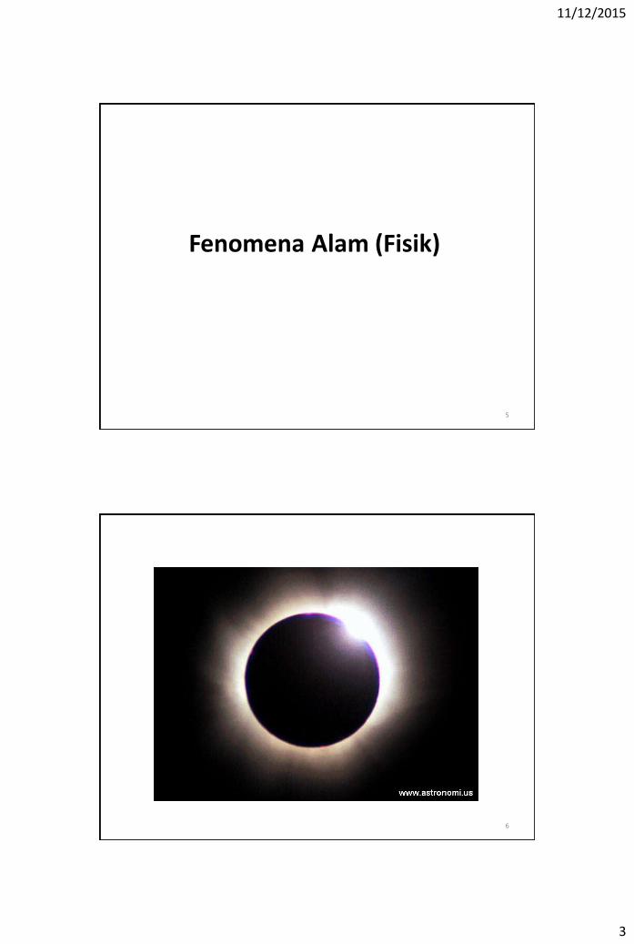
Fenomena Alam (Fisik)

5

6

11/12/2015

4

7

8

11/12/2015

5

9

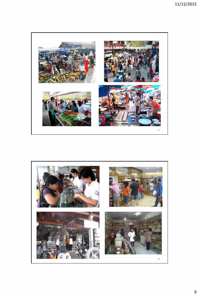
Fenomena Sosial

10

11/12/2015

6

11

12

11/12/2015

7

13

14

11/12/2015

8

15

16

11/12/2015

9

17

18

11/12/2015

10

19

20

11/12/2015

11

21

22

11/12/2015

12

Tabel Produksi dan Konsumsi Beras Nasional

Tahun Produksi Konsumsi

1983 25932 24679

1984 24006 25460

1985 26542 26092

1986 27014 26738

1987 27253 27392

1988 28340 28053

1989 29072 28723

1990 29366 29410

1991 29047 30121

1992 31356 30838

1993 31318 31375

1996 33216 33461

1997 31206 33911

Catatan historis dinamika (behavior) perberasan nasional

23

Tabel Produksi dan Konsumsi Beras Nasional

Tahun Produksi Konsumsi

1998 31118 34667

1999 31294 35033

2000 32130 35400

2001 31891 35877

2002 32130 36382

2003 32950 36500

2004 33940 36000

2005 34120 35850

2006 34600 35739

2007 36350 35900

2008 38078 37100

2009 40656 37400

24

11/12/2015

13

Dinamika (Perilaku) Produksi dan Konsumsi Beras Nasional

0

5000

10000

15000

20000

25000

30000

35000

40000

45000

Rib

u T

on

Tahun

Produksi

Konsumsi

25

Suatu fenomena menyangkut 2 hal (aspek):

(1) Struktur (structure) Perilaku (behavior) (2)

(unsur pembentuk fenomena dan pola keterkaitan antar unsur tersebut)

(perubahan suatu besaran/variabel dalam suatu kurun waktu tertentu, baik kuantitatif maupun kualitatif)

C

A

D B

Tahun

Produksi padi (ton/tahun)

Fenomena sosial : struktur fisik; dan struktur pembuatan keputusan.

Pemahaman hubungan struktur dan perilaku sangat diperlukan dalam mengenali suatu fenomena.

26

11/12/2015

14

1.2 Sistem

Suatu sistem adalah suatu fenomena yang strukturnya telah diketahui [A phenomenon which its structure has been defined].

Atau

Suatu sistem merupakan suatu gabungan dari beberapa bagian yang bekerja untuk tujuan bersama. Suatu sistem dapat terbentuk dari sejumlah orang dan/atau sejumlah komponen fisik [A system means a grouping of parts that operate together for common purpose. A system may include people as well as physical parts].

27

1.3 Persoalan (Problem)

• Suatu fenomena yang kehadirannya tidak diinginkan, contoh: produktivitas padi yang terus menurun, tingkat pengangguran yang terus bertambah.

• Suatu fenomena yang ingin diwujudkan. Contoh: suatu target surplus beras yang ingin dicapai pada tahun 2014.

• (secara praktis) Suatu kesenjangan (gap) antara keadaan sebenarnya (actual state) dengan keadaan yang diinginkan (goal).

28

11/12/2015

15

1.4 Contoh Kasus

To achieve the intended level of rice production (higher level of self-sufficiency in rice production, currently is about 65-75% of domestic consumption), Malaysia implements a wide range of market intervensions. The policy instruments include among others:

• A guaranteed minimum price for paddy;

• Various cash and input subsidies to farmers and millers;

• Import monopoly; and

• Price control for rice.

(Sumber: Tesis Emmy Farha Binti Alias, Universiti Putra Malaysia, 2013)

29

Figure 1.4.1 Planted Paddy area (‘000 ha) and Productivity (t/ha/year) [Source: DoS(2010)]

30

11/12/2015

16

Figure 1.4.2 SSL(%) and Fertilizer Subsidy (RM mn/year), 1990-2008 [Source: MoA(2010)]

31

Figure 1.4.3 The Global Model

For the future, Malaysia needs to dismantle all the policy instruments to comply with the WTO agreement.

32

11/12/2015

1

Sesi 2 Struktur, Perilaku, dan Analisis

Kebijakan

1

Outcomes

Pada akhir sesi ini, peserta dapat:

• memahami 2 aspek suatu fenomena (struktur dan perilaku);

• mengenali struktur fisik dan struktur pembuatan keputusan;

• memahami konsep kompleksitas; dan

• memahami prinsip suatu analisis kebijakan (policy analysis).

2

11/12/2015

2

2.1 Dua Aspek Suatu Fenomena (1) Struktur (structure) Perilaku (behavior) (2)

(unsur pembentuk fenomena dan pola keterkaitan antar unsur tersebut)

(perubahan suatu besaran/variabel dalam suatu kurun waktu tertentu, baik kuantitatif maupun kualitatif)

C

A

D B

Tahun

Produksi padi (ton/tahun)

Fenomena sosial : struktur fisik; dan struktur pembuatan keputusan.

Pemahaman hubungan struktur dan perilaku sangat diperlukan dalam mengenali suatu fenomena.

3

A Picture of an Economy

• Households, firms, and governments make economic decisions. Households decide how much of their labor, land, capital, and entrepreneurial ability to sell or rent in exchange for wages, rent, interest, and profits. They also decide how much of their income to spend on the various types of goods and services available. Firms decide how much labor, land, and capital to hire and how much of the various types of goods and services to produce. Governments decide which goods and services they will provide and the taxes that households and firms will pay.

• These decisions by households, firms, and

governments are coordinated in markets—the goods market and factor markets—that are regulated by rules that governments establish and enforce. In these markets, prices constantly adjust to keep buying and selling plans consistent.

4

11/12/2015

3

Contoh : Pengisian air ke dalam gelas sampai penuh. (Sumber: “The Fifth Discipline”, Peter M. Senge, 1990)

5

Kemungkinan Perilaku

A. Jika sumber air mencukupi

0

1

2

3

4

5

6

7

8

0 1 2 3 4 5 6 7 8 9 10

Volume air dalam gelas

Aliran air ke

dalam gelas

Volume air dalam gelas yang diinginkan

6

11/12/2015

4

Kemungkinan Perilaku

B. Jika sumber air terbatas

0

1

2

3

4

5

6

7

8

0 1 2 3 4 5 6 7 8 9 10

Aliran air ke

dalam gelas

Volume air dalam gelas yang diinginkan

Volume air dalam gelas

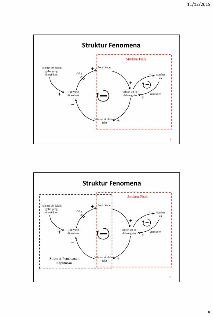
7

Gap yang

dirasakan

Aliran air ke

dalam gelas

Posisi keran

Volume air dalam

gelas

Volume air dalam

gelas yang

diinginkan delay Sumber

air

Struktur Fenomena

nonlinier

8

11/12/2015

5

Gap yang

dirasakan

Aliran air ke

dalam gelas

Posisi keran

Volume air dalam

gelas

Volume air dalam

gelas yang

diinginkan delay Sumber

air

Struktur Fisik

Struktur Fenomena

nonlinier

9

Gap yang

dirasakan

Aliran air ke

dalam gelas

Posisi keran

Volume air dalam

gelas

Volume air dalam

gelas yang

diinginkan delay Sumber

air

Struktur Fisik

Struktur Pembuatan

Keputusan

Struktur Fenomena

nonlinier

10

11/12/2015

6

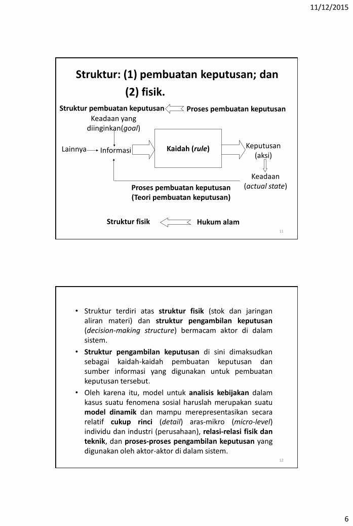
Struktur: (1) pembuatan keputusan; dan

(2) fisik. Struktur pembuatan keputusan Proses pembuatan keputusan

Kaidah (rule)

Informasi

Keputusan (aksi)

Proses pembuatan keputusan (Teori pembuatan keputusan)

Struktur fisik Hukum alam

Keadaan (actual state)

Keadaan yang diinginkan(goal)

Lainnya

11

• Struktur terdiri atas struktur fisik (stok dan jaringan aliran materi) dan struktur pengambilan keputusan (decision-making structure) bermacam aktor di dalam sistem.

• Struktur pengambilan keputusan di sini dimaksudkan sebagai kaidah-kaidah pembuatan keputusan dan sumber informasi yang digunakan untuk pembuatan keputusan tersebut.

• Oleh karena itu, model untuk analisis kebijakan dalam kasus suatu fenomena sosial haruslah merupakan suatu model dinamik dan mampu merepresentasikan secara relatif cukup rinci (detail) aras-mikro (micro-level) individu dan industri (perusahaan), relasi-relasi fisik dan teknik, dan proses-proses pengambilan keputusan yang digunakan oleh aktor-aktor di dalam sistem.

12

11/12/2015

7

• Exponential Growth

• Goal Seeking

• S-Shaped Growth

• Oscillation

• Growth with Overshoot

• Overshoot and Collapse

2.2 Pola Karakteristik Perilaku Sistem

13

2.3 Konsep Kompleksitas (Sterman, J.D., Business Dynamics: Systems Thinking and Modeling for a Complex World, 2004, Mc Graw HIll)

(1) Struktur Perilaku (2)

(unsur pembentuk fenomena dan pola

keterkaitan antar unsur tersebut)

(perubahan suatu besaran/variabel

dalam suatu kurun waktu tertentu, baik

kuantitatif maupun kualitatif)

C

A

D B

Waktu

Orang Miskin

(A)

Fenomena Sosial: Struktur fisik; dan struktur pembuatan keputusan.

14

11/12/2015

8

• Detail complexity

Complexity in terms of the number of elements (components) in a phenomenon (system), or the number of combinations one must consider in making a decision.

• Dynamic complexity (Kompleksitas Dinamis)

Arises from the relationships (interactions) among the agents (elements) over time.

15

Kompleksitas dinamis muncul karena fenomena mempunyai karakteristik:

• Dynamic Heraclitus said, “All is change.” What appears to be unchanging is, over alonger time horizon, seen to vary. Change in systems occurs at many time scales, and these different scales sometimes interact. A star evolves over billions of years as it burns its hydrogen fuel, then can explode as a supernova in seconds. Bull markets can go on for years, then crash in a matter of hours.

• Tightly coupled The actors in the system interact strongly with one another and with the natural world. Everything is connected to everything else. As a famous bumper sticker from the 1960s proclaimed, “You can’t do just one thing.”

16

11/12/2015

9

• Governed by feedback Because of the tight couplings among actors, our actions feed back on themselves. Our decisions alter the state of the world, causing changes in nature and triggering others to act, thus giving rise to a new situation which then influences our next decisions. Dynamics arise from these feedbacks.

• Nonlinier Effect is rarely proportional to cause, and what happens locally in a system (near the current operating point) often does not apply in distant regions (other states of the system). Nonlinearity often arises from the basic physics of systems: Insufficient inventory may cause you to boost production, but production can never fall below zero no matter how much excess inventory you have. Nonlinearity also arises as multiple factors interact in decision making: Pressure from the boss for greater achievement increases your motivation and effort-up to the point where you perceive the goal to be impossible. Frustration then dominates motivation and you give up or get a new boss.

17

• History-dependent Taking one road often precludes taking others and determines where you end up (path dependence). Many actions are irreversible: You can’t unscramble an egg (the second law of thermodynamics). Stocks and flows (accumulations) and long time delays often mean doing and undoing have fundamentallydifferent time constants: During the 50 years of the Cold War arms race the nuclear nations generated more than 250 tons of weapons-grade plutonium (239Pu)T. he half life of 239Pu is about 24,000 years.

• Self Organizing The dynamic of systems arise spontaneously from their internal structure. Often, small, random pertubations are amplified and molded by feedback structure, generating patterns in space and time and creating path dependence.The pattern of stripes on a zebra, the rhythmic contraction of your hearth, the persistent cycles in the real estate market, and structures such as sea shells and markets all emerge spontaneously from the feddbacks among the agents and elements of the system.

18

11/12/2015

10

• Adaptive The capabilities and decision rules of the agents in complex systems change over time. Evolution leads to selection and proliferation of some agents while others become extinct. Adaptation also occurs as people learn from experience, especially as they learn new ways to achieve their goals in the face of obstacles. Learning is not always beneficial, however.

• Counterintuitive In complex systems cause and effect are distant in time and space while we tend to look for causes near the events we seek to explain. Our attention is drawn to the symptoms of difficulty rather than the underlying cause. High leverage policies are often not obvious.

• Policy resistant The complexity of the systems in which we are embedded over whelms our ability to understand them. The result: Many seemingly obvious solutions to problems fail or actually worsen the situation.

19

• Characterized by trade-offs Time delays in feedback channels mean the long-run response of a system to an intervention is often different from its short-run response. High leverage policies often cause worse-before-better behavior, while low leverage policies often generate transitory improvement before the problem grows worse.

20

11/12/2015

11

2.4 Pertanyaan Terhadap Perilaku (Fenomena)

(a) Berapakah nilai (angka) besaran itu pada suatu titik

waktu yang akan datang? [point prediction]

(prakiraaan, prediksi masa depan)

(b) Mengapa perubahan besaran tersebut seperti itu?

(why ?) Dan dengan cara bagaimanakah

mengubahnya? (how ?) [behavior prediction]

(menyusun strategi dan memformulasikan kebijakan,

analisis kebijakan atau policy analysis)

21

Contoh: Dinamika Produksi Gula di Indonesia

22

11/12/2015

12

2.5 Strategi dan Kebijakan

Tujuan

Strategi

Program

Aktivitas

diwujudkan dengan

diimplementasikan melalui berbagai

direalisasikan dengan melaksanakan

•Policy statements •Policy instruments •Policy measures

Kebijakan

diungkapkan dalam bentuk

Menci

pta

kan k

ondis

i &

iklim

yang m

endukung

perw

uju

dan d

an p

ela

ksa

naan

23

• Strategi (strategy)

Sebuah rencana (metode) aksi untuk mencapai suatu tujuan tertentu [a plan (method) of action to achieve a particular goal (aim)]

24

11/12/2015

13

Kebijakan

• menciptakan serta membangun iklim dan kondisi yang perlu untuk mendukung (to facilitate) pelaksanaan strategi;

• memberikan kepastian kepada unsur-unsur dunia usaha, masyarakat luas, dan peyelenggara pemerintahan; tentang arah, ruang lingkup, dan tingkat keleluasaan masing-masing di dalam memilih upaya yang berkaitan dengan strategi tersebut.

Petunjuk-petunjuk (directives) yang dikeluarkan dan disebarluaskan (oleh pemerintah) dengan tujuan:

25

Pelaksanaan Kebijakan

Untuk melaksanakan kebijakan, setelah mengeluarkan kebijakan (pernyataan), policy measures harus dibentuk:

• bentuk, rumuskan, dan keluarkan instrumen-instrumen kebijakan (hukum, peraturan, petunjuk-petunjuk);

• bentuk dan dirikan badan-badan administratif dan prosedur-prosedur untuk mencatat (to administer) kegiatan-kegiatan yang berkaitan dengan pelaksanaan kebijakan; dan

• alokasikan sumberdaya (dana, manusia, fasilitas) untuk mendukung badan administratif di atas.

26

11/12/2015

14

Proses Pendekatan Perumusan Kebijakan

'KE

BIJ

AK

AN

'

[ K

]

Ori

en

tatif, P

reskri

ptif

Info

rmasi

yan

g r

ele

van

(Basis

in

form

asi u

ntu

k m

en

gid

en

tifikasi d

an

mem

form

ula

sik

an

T,S

, P,

dan

K)

'TUJUAN'

[ T ]

Deskriptif

Orientatif

'STRATEGI'

[ S ]

Preskriptif

'PROGRAM'

[ P ]

Preskriptif

informasi

informasi

informasi

Ara

han

-ara

han

yan

g p

erlu

un

tuk

men

du

kung

S &

P

Pengamatan analitik tentang dunia nyata

(deskriptif)

Kegiatan dan

rencana untuk

merealisasikan

strategi

Arahan dasar bagi

tindakan untuk

mencapai tujuan

Keinginan ( desired ) yang

ingin dicapai

27

Kebijakan Publik [Wibawa, Samodra (2011), Politik Perumusan Kebijakan Publik, Graha Ilmu –

Yogyakarta]

Kebijakan publik adalah keputusan suatu “sistem politik”

negara, provinsi, kabupaten dan desa, atau RW dan RT

untuk/dalam/guna mengelola suatu masalah (persoalan)

atau memenuhi suatu kepentingan publik, di mana

pelaksanaan keputusan itu membutuhkan dikerahkannya

sumberdaya milik semua warga (publik) sistem politik

tersebut.

[UUD, Keppres, Permen, Perdes (Peraturan desa),

ataupun peraturan RT (Rumah Tangga)]

28

11/12/2015

15

Ability to intervene (create changes)

Events

Patterns

Structure

• Fenomena Gunung Es (The Iceberg Phenomenon) Fenomena gunung es (the iceberg) ini menggambarkan bahwa sturktur yang sistematis merupakan fondasi terbentuknya suatu pola (patterns) dan kejadian (events). Namun struktur sistematis tersebut sulit untuk dilihat. Sering kali kita hanya melihat kejadiannya saja (puncak dari gunung es), dan hal tersebut menjadi dasar pengambilan keputusan. Padahal kejadian (events) hanyalah merupakan akibat (hasil) suatu struktur. Sehingga keputusan yang dibuat berdasarkan kejadian (events) tidak akan menyelesaikan suatu persoalan.

2.6 Logical framework (approach)

(Sumber: Innovation Associates) 29

Reaktif

Saat ini

Mengamati kejadian

“Bagaimana cara tercepat untuk

merespon kejadian ini?”

Adaptif

Mengamati pola perubahan

kejadian

“Seperti apa kecenderungan dan pola dari

kejadian tersebut, apakah

terdapat pengulangan?”

Perubahan

Masa depan

Causal loop diagrams dan

metode systems thinking lainnya

“Struktur seperti apakah yang

menyebabkan terbentuknya

pola tersebut?”

Kejadian

Struktur

Pola

Tindakan Waktu Cara

Pemahaman Pertanyaan yang dapat diajukan

• Tingkatan Pemahaman (Levels of understanding)

Sumber : Anderson, Virginia and Lauren Johnson, 1997: Systems Thinking Basics: From Concepts to Causal Loops, Pegasus Communications, Inc. MA USA.

30

11/12/2015

16

2.7 Model Untuk Analisis Kebijakan

31

Unknown process

Real world

decisions Real world

history

Model

structure Model

behavior

• Pemodelan kebijakan (policy modelling)

Kerangka Pemikiran (Pendekatan)

Policy (intervention)? Real world (fenomena)

Model

Simulation

32

11/12/2015

17

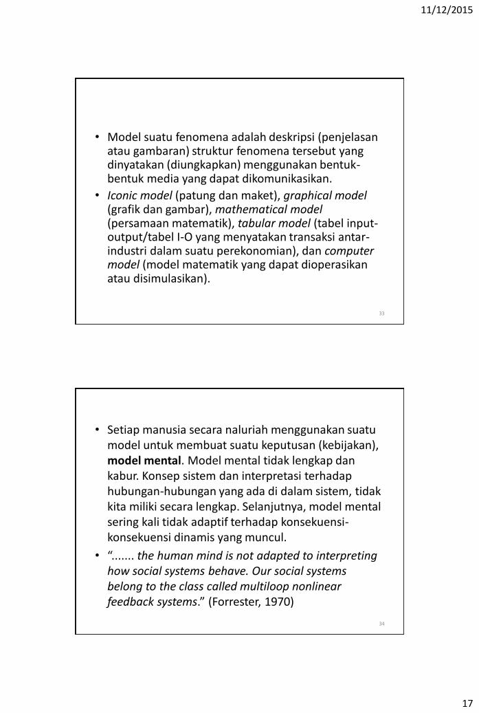
• Model suatu fenomena adalah deskripsi (penjelasan atau gambaran) struktur fenomena tersebut yang dinyatakan (diungkapkan) menggunakan bentuk-bentuk media yang dapat dikomunikasikan.

• Iconic model (patung dan maket), graphical model (grafik dan gambar), mathematical model (persamaan matematik), tabular model (tabel input-output/tabel I-O yang menyatakan transaksi antar-industri dalam suatu perekonomian), dan computer model (model matematik yang dapat dioperasikan atau disimulasikan).

33

• Setiap manusia secara naluriah menggunakan suatu model untuk membuat suatu keputusan (kebijakan), model mental. Model mental tidak lengkap dan kabur. Konsep sistem dan interpretasi terhadap hubungan-hubungan yang ada di dalam sistem, tidak kita miliki secara lengkap. Selanjutnya, model mental sering kali tidak adaptif terhadap konsekuensi-konsekuensi dinamis yang muncul.

• “....... the human mind is not adapted to interpreting how social systems behave. Our social systems belong to the class called multiloop nonlinear feedback systems.” (Forrester, 1970)

34

11/12/2015

18

Keputusan berdasarkan model mental,

35

hasil yang tidak diharapkan!

Dibutuhkan suatu model eksplisit ???

36

11/12/2015

19

Prinsip-Prinsip Pemodelan Kebijakan

• Model yang memenuhi syarat dan mampu dijadikan sarana analisis untuk merumuskan (merancang) kebijakan haruslah merupakan suatu wahana untuk menemukan jalan dan cara intervensi yang efektif dalam suatu sistem (fenomena).

• Melalui jalan dan cara intervensi inilah perilaku sistem yang diinginkan dapat diperoleh (perilaku sistem yang tidak diinginkan dapat dihindari).

• Model yang dibentuk untuk tujuan seperti di atas haruslah memenuhi syarat-syarat berikut:

37

• karena efek suatu intervensi (kebijakan), dalam bentuk perilaku, merupakan suatu kejadian berikutnya; maka untuk melacaknya, unsur (elemen) waktu perlu ada (dynamic);

• mampu mensimulasikan bermacam intervensi dan dapat memunculkan perilaku sistem karena adanya intervensi tersebut;

• memungkinkan mensimulasikan suatu intervensi yang efeknya dapat berbeda secara dramatik: (1) dalam konteks waktu (efek jangka pendek vs jangka panjang, trade offs in time), dan (2) dalam konteks sektoral (efek memperbaiki performance suatu sektor yang berakibat memperburuk performance sektor yang lain, trade offs between sectors); disebut dengan istilah dynamic complexity (kompleksitas dinamik);

• perilaku sistem di atas dapat merupakan perilaku yang pernah dialami dan teramati (historis) ataupun perilaku yang belum pernah teramati (pernah dialami tetapi tidak teramati atau belum pernah dialami tetapi kemungkinan besar terjadi); dan

• mampu menjelaskan mengapa (why) suatu perilaku tertentu (transisi yang sukar misalnya) dapat terjadi.

38

11/12/2015

20

• Keadaan yang diinginkan dan keadaan yang terjadi harus secara eksplisit dinyatakan dan dibedakan di dalam model;

• Adanya struktur stok dan aliran dalam kehidupan nyata harus dapat direpresentasikan di dalam model;

• Aliran-aliran yang secara konseptual berlainan cirinya harus secara tegas dibedakan di dalam menanganinya;

• Hanya informasi yang benar-benar tersedia bagi aktor-aktor di dalam sistem yang harus digunakan dalam pemodelan keputusan-keputusannya;

• Struktur kaidah pembuatan keputusan di dalam model haruslah sesuai (cocok) dengan praktek-praktek manajerial; dan

• Model haruslah robust dalam kondisi-kondisi ekstrem.

Prinsip-Prinsip Membuat Model Dinamik (Sterman, 1981)

39

Kesahihan (validity) Model

• Dalam hubungannya dengan kesahihan (validity) model, suatu model haruslah sesuai (cocok) dengan kenyataan empirik (realitas) yang ada.

• Model merupakan hasil dari suatu upaya untuk membuat tiruan kenyataan tersebut (Burger, 1966).

• Upaya pemodelan haruslah memenuhi (sesuai dengan) metode ilmiah. Saeed (1984) telah melukiskan metode ilmiah ini berdasarkan kepada konsep penyangkalan (refutation) Popper (1969).

• Metode ini menyaratkan bahwa suatu model haruslah mempunyai banyak titik kontak (points of contact) dengan kenyataan (reality) dan pembandingan yang berulang kali antara model dengan dunia nyata (real world) melalui titik-titik kontak tersebut haruslah membuat model menjadi robust.

40

11/12/2015

21

Patterns recognized

Decision rules experienced

Induction

Contact point for comparison

Unknown process

Real world

decisions Real world

history

Model

structure Model

behavior

Deductive logic

Metode Ilmiah (Saeed, 1984)

(epistemological: how our knowledge claims could be justified)

41

Usaha pertama dari penyelidikan ilmiah adalah upaya untuk memahami bagaimana suatu perilaku dunia nyata muncul dari strukturnya. Karena tidak ada cara langsung yang dapat digunakan untuk mengetahuinya, suatu model yang mewakili struktur dunia nyata itu harus dikonstruksikan dan perilakunya kemudian diperoleh melalui logika deduktif. Struktur model ini didapat melalui suatu proses induksi yang didasarkan kepada pengetahuan empirik tentang dunia nyata tersebut. Pembandingan-pembandingan baik struktur maupun perilaku model dengan struktur dan perilaku dunia nyata akan menegakkan kepercayaan dalam model, dan pada gilirannya kepercayaan itu akan menjadi dasar kesahihan model tersebut (Kemeny, 1959).

42

11/12/2015

22

FENOMENA

ANALISIS

STRUKTUR •unsur pembentuk

•pola keterkaitan

FUNGSI-FUNGSI

YANG DAPAT

DITEGAKKAN

POLA LAKU

(behavior pattern)

MEMANFAATKAN

MENGOPERASIKAN

MENGENDALIKAN

MEMBENTUK ATAU

MENCIPTAKAN

STRUKTUR-

STRUKTUR BARU

DGN MENGUBAH

STRUKTUR ATAU

MENSINTESIS DGN

STRUKTUR LAIN

METODOLOGI

Dengan melakukan

diketahui

Dapat

dilacak

dan

diketahui

Dapat

dilacak

dan

digagas-

kan cara

untuk

Sumber: Sasmojo (2000)

Analisis

FENO

MENA

LAIN

43

Dua (2) kesukaran: 1) menentukan batas-batas model (model boundary); dan 2) menentukan struktur pembuatan keputusan.

Saeed (1982): • Pendekatan kotak hitam (black box approach), hubungan-

hubungan struktural biasanya dicari melalui suatu proses deduksi dari data historis tentang perilaku sistem. Penentuan variabel-variabel yang penting yang harus masuk dalam model ditentukan melalui pengujian-pengujian statistik berdasarkan data historis perilaku sistem tersebut.

Menurut Black (1982), pendekatan ini sering menimbulkan kesalahan-kesalahan spesifikasi dan identifikasi struktur sistem; karena adanya penyimpangan (bias) data.

44

11/12/2015

23

Alternatif lain adalah memodelkan struktur proses pembuatan keputusan aktor-aktor dalam sistem (fenomena) berdasarkan struktur informasi sistem yang di dalamnya terdapat aktor-aktor, sumber-sumber informasi, dan jaringan aliran informasi yang menghubungkan keduanya.

• analogi fisik, sumber informasi merupakan suatu tempat penyimpanan (storage/stock), sedangkan keputusan merupakan aliran yang masuk ke atau keluar dari tempat penyimpanan itu.

• analogi matematik, sumber informasi dinyatakan sebagai variabel keadaan (state variable), sedangkan keputusan merupakan turunan (derivative) variabel keadaan tersebut.

45

Proses Pembuatan Keputusan

Informasi yang

terakumulasi

dalam sistem

Informasi

baru yang

muncul

Aksi-aksi

Aktor-aktor

Informasi lingkungan

Pembaharuan informasi

46

11/12/2015

24

Struktur: (1) pembuatan Keputusan; dan

(2) fisik. Struktur pembuatan keputusan Proses pembuatan keputusan

Kaidah (rule)

Informasi

Keputusan (aksi)

Proses pembuatan keputusan (Teori pembuatan keputusan)

Struktur fisik Hukum alam

Keadaan (actual state)

Keadaan yang diinginkan(goal)

Lainnya

47

Proses pembuatan keputusan menyangkut fenomena-fenomena yang dinamis. Fenomena dinamis ini dimunculkan oleh adanya struktur fisik dan struktur pembuatan keputusan yang saling berinteraksi. • Struktur fisik dibentuk oleh akumulasi (stok) dan jaringan

aliran orang, barang, energi, dan bahan. • Struktur pembuatan keputusan dibentuk oleh akumulasi

(stok) dan jaringan aliran informasi yang digunakan oleh aktor-aktor (manusia) dalam sistem yang menggambarkan kaidah-kaidah proses pembuatan keputusannya.

Struktur fisik dan struktur pembuatan keputusan

48

12/11/2015

1

Sesi 3 Inventory Simulation Game

1

Outcomes

Memahami bahwa struktur (fisik dan pengambilan keputusan) menentukan perilaku

2

12/11/2015

2

3.1 The Inventory Game (1) • The Inventory Game is one of a number of

management simulators developed at MIT's Sloan School of Management for these purposes. The game was developed by Sloan's System Dynamics Group in the early 1960s as part of Jay Forrester's research on industrial dynamics. Its has been played all over the world by thousands of people ranging from high school students to chief executive officers and government officials.

• The game is played by teams of at least four players, often in heated competition, and takes from one to one and a half hours to complete. A debriefing session of roughly equivalent length typically follows to review the results of each team and discuss the lessons involved.

3

The Inventory Game (2) • The purpose of the game is to understand the distribution

side dynamics of a multi-echelon supply chain used to distribute a single item. The aim is to meet customer demand of goods through the distribution side of a multi-stage supply chain with minimal expenditure on back orders and inventory.

• Players can see each other's inventory but only one player sees actual customer demand. Verbal communication between players is against the rules so feelings of confusion and disappointment are common.

• Players look to one another within their supply chain frantically trying to figure out where things are going wrong. Most of the players feel frustrated because they are not getting the results they want.

• Players wonder whether someone in their team did not understand the game or assume customer demand is following a very erratic pattern as backlogs mount and/or massive inventories accumulate.

4

12/11/2015

3

The Inventory Game (3)

• Suatu ilustrasi yang memperlihatkan bahwa perilaku suatu fenomena (sistem) ditentukan terutama oleh struktur internalnya.

Flow of Goods

5

• Setiap policy-maker mempunyai kebebasan sepenuhnya untuk menentukan ordering policy dalam aturan-aturan sebagai

berikut ini. 1. Pengiriman barang harus memenuhi semua order, sepanjang stok

barang dalam inventory memungkinkan untuk keperluan itu. 2. Diberlakukan struktur biaya (cost):

o Carrying cost adalah $ 0.50 per unit/period; dan o Out-of stock costs adalah $ 2.00 per unit/period.

• Agar biaya total minimum, setiap sektor dalam sistem harus

berupaya menjaga agar stok dalam inventory-nya seminimum mungkin, tetapi cukup untuk dapat memenuhi permintaan yang boleh jadi berubah.

• Bila stok lebih kecil dari kebutuhannya, order harus lebih besar

dari tingkat penjualan (pengiriman) rata-rata. Sebaliknya, bila stok lebih besar dari kebutuhannya, order harus lebih kecil dari penjualan (pengiriman) rata-rata. 6

12/11/2015

4

• Setiap policy-maker harus dapat menjawab 2 (dua) pertanyaan berikut ini.

1. Apakah stok yang dimiliki dalam inventory cukup untuk memenuhi permintaan? (kenyataan)

2. Berapa banyak barang yang harus dipesan ke pemasok dan cukup untuk menghindari terjadinya out-of-stock?

(kebijakan atau policy)

7

3.2 Langkah-Langkah Permainan Langkah 1

a. Kirim barang dari inventory ke sektor sebelah kiri, sesuai dengan permintaan yang tertera di order backlog. Barang diletakkan pada bagian kanan shipping delay sektor sebelah kiri. Bila barang yang harus dikirim tidak tersedia simpan secarik kertas sebagai penanda. (Untuk sektor retailer simpan barang terkirim pada customers decks, sedangkan sektor factory kirim seluruh barang yang berada di inventory ke distributor).

b. Jika pengiriman sesuai dengan permintaan, buang catatan pesanan dari order backlog. Jika pengiriman tidak sesuai dengan permintaan, catat kekurangan pengiriman dengan menambahkannya pada order backlog.

Langkah 2: Catat jumlah inventory dan order backlog pada formulir yang telah disediakan.

Langkah 3: Pindahkan barang-barang pada bagian kirim shipping delay ke inventory.

Langkah 4: Pindahkan barang-barang dari sebalah kanan ke sebelah kiri dari shipping delay [termasuk memindahkan barang pada sektor factory: 4(a) and 4(b)].

Langkah 5:Tentukan jumlah barang yang akan dipesan, dan simpan pada bagian kiri dari mail box di sektor sebelah kanan.

Langkah 6: Catat pesanan pada formulir yang disediakan.

Langkah 7: Ambil pesanan di mail box, tambahkan dengan jumlah yang tertera di order backlog. ( Sektor retailer ambil pesanan dari orders deck, sedangkan sektor factory langsung memproduksi barang sesuai dengan permintaan dan simpan pada bagian atas dari kotak goods in process).

Langkah 8: Pindahkan slip order dari kiri delay bagian kanan delay mail box.

Langkah 9: Kembali ke langkah pertama.

8

12/11/2015

5

Orders deck

Order backlog

2 (Record backlog)

1(b) Order

discard rate

5 (Order rate)

Inventory

Shipping delay

2 (Record inventory)

Customers deck

3

4

RETAILER

1(a)

7

6 (Record order)

9

Order backlog

2 (Record backlog)

1(b) Order

discard rate

5 (Order rate)

Inventory

Shipping delay

2 (Record inventory)

3

4

WHOLESALER

1 (a)

7

Mail delay

8

Shipments to retailer

6 (Record order)

10

12/11/2015

6

Order backlog

2 (Record backlog)

1(b) Order

discard rate

5 (Order rate)

Inventory

Shipping delay

2 (Record inventory)

3

4

DISTRIBUTOR

1 (a)

7

Mail delay

8

Shipments to wholesaler

6 (Record order)

11

Inventory

2 (Record inventory)

FACTORY

1 (a)

Mail delay

8

Goods In process

7

4 (b)

4 (a)

Orders from distributor

Shipments to distributor

12

11/12/2015

1

Sesi 4 Systems Thinking

& System Dynamics

1

Outcomes

Pada akhir sesi ini, peserta dapat:

• mengenali hubungan sebab akibat;

• memahami metodologi pemodelan system dynamics.

2

11/12/2015

2

Pengisian air ke dalam gelas sampai penuh (Sumber: “The Fifth Discipline”, Peter M. Senge, 1990)

3

Kemungkinan Perilaku

A. Jika sumber air mencukupi

0

1

2

3

4

5

6

7

8

0 1 2 3 4 5 6 7 8 9 10

Volume air dalam gelas

Aliran air ke

dalam gelas

Volume air dalam gelas yang diinginkan

4

11/12/2015

3

Kemungkinan Perilaku

B. Jika sumber air terbatas

0

1

2

3

4

5

6

7

8

0 1 2 3 4 5 6 7 8 9 10

Aliran air ke

dalam gelas

Volume air dalam gelas yang diinginkan

Volume air dalam gelas

5

Gap yang

dirasakan

Aliran air ke

dalam gelas

Posisi keran

Volume air dalam

gelas

Volume air dalam

gelas yang

diinginkan delay Sumber

air

Struktur Fenomena

nonlinier

6

11/12/2015

4

Gap yang

dirasakan

Aliran air ke

dalam gelas

Posisi keran

Volume air dalam

gelas

Volume air dalam

gelas yang

diinginkan delay Sumber

air

Struktur Fisik

Struktur Fenomena

nonlinier

7

Gap yang

dirasakan

Aliran air ke

dalam gelas

Posisi keran

Volume air dalam

gelas

Volume air dalam

gelas yang

diinginkan delay Sumber

air

Struktur Fisik

Struktur Pembuatan

Keputusan

Struktur Fenomena

nonlinier

8

11/12/2015

5

Metodologi Pemodelan

Struktur Perilaku unsur pembentuk

pola keterkaitan antar unsur :

(1) feedback (causal loop) (2) stock (level) dan flow (rate) (3) delay (4) nonlinearity (ontological: the ways reality itself could be)

Pendekatan Struktural Systems Thinking System Dynamics

Systems Thinking dan System Dynamics

9

4.1 System Dynamics Methodology

10

11/12/2015

6

A. Source: System Dynamics Home Page.htm

11

System Dynamics Methodology

• System dynamics is a methodology for studying and managing complex feedback systems, such as one finds in business and other social systems.

• In fact it has been used to address practically every sort of feedback system.

• While the word system has been applied to all sorts of situations, feedback is differentiating descriptor here.

• Feedback refers to the situation of X affecting Y and Y in turn affecting X perhaps through a chain of causes and effects.

• One cannot study the link between X and Y and, independently, the link between Y and X and predict how the system behave. Only the study of the whole system as a feedback system will lead to correct results.

12

11/12/2015

7

What is the relationship of

Systems Thinking to System Dynamics?

• Systems thinking looks at the same type of problems from the same perspective as does system dynamics.

• The two techniques share the same causal loop mapping techniques.

• System dynamics takes the additional step of constructing computer simulation models to confirm that the structure hypothesized can lead to the observed behavior and to test the effects of alternative policies on key variables over time.

13

B. Source:

Richardson, George P. & Alexander L. Pugh III

(1981), Introduction to System Dynamics Modeling

with Dynamo, MIT Press/Wright-Allen series in

system dynamics.

14

11/12/2015

8

Overview of the System Dynamics Approach

• The system dynamics approach to complex problems focuses on feedback processes. It takes the philosophical position that feedback structures are responsible for the changes we experience over time. The premise is that dynamic behavior is consequence of system structure and will become meaningful and powerful. At this point, it may be treated as a postulate, or perhaps as a conjecture yet to be demonstrated.

• As both a cause and a consequence of the feedback perspective, the system dynamics approach tends to look within a system for the sources of its problem behavior. Problems are not seen as being caused by external agents outside the system.

15

• Inventories are not assumed to oscillate merely because consumers periodically vary their orders. A ball does not bounce merely because someone drops it. A pendulum does not oscillate merely because it was displaced from the vertical. The system dynamicist prefers to take the point of view that these systems behave as they do for reasons internal to each system. A ball bounces and a pendulum oscillates because there is something about their internal structure that gives them the tendency to bounce or oscillate.

• In practice, this internal point of view results in models of feedback system that bring external agents inside the system. Customers orders become endogenous to a production system, part of the feedback structure of the system. Orders affect production; production affects orders. Part and parcel with the notion of feedback, the endogenous point of view helps to characterize the system dynamics approach. 16

11/12/2015

9

• The are roughly seven stages in approaching a problem from the system dynamics perspective:

(1) problem identification and definition;

(2) system conceptualization;

(3) model formulation;

(4) analysis of model behavior;

(5) model evaluation;

(6) policy analysis; and

(7) model use or implementation.

17

• The process begins and ends with understandings of a system and its problems, so it forms a loop, not a linear progression. Figure 4.1 shows these stages and the likely progression through them, together with some arrows that represent the cycling, iterative nature of the process. At a number of stages along the way one’s understanding of the system and the problem are enhanced by the modeling process, and that increased understanding further aids the modeling effort.

• Figure 4.1 shows that final policy recommendations from a system dynamics study come not merely from manipulations with the formal model but also from the additional understandings one gains about the real system by iterations at a number of stages in the modeling process. Done properly, a system dynamics study should produce policy recommendations that can be presented, explained, and defended without resorting to the formal model. The model is a means to an end, and that end is understanding.

18

11/12/2015

10

Figure 4.1 Overview of the system dynamics modeling approach

Policy implementation

Understanding of a system

Policy analysis

Simulation

Model formulation

System conceptualization

Problem definition

19

Guidelines for Causal-loop Diagrams

1. Think of variables in causal-loop diagrams as quantities that can rise or fall, grow or decline, or be up or down. But do not worry if you can not readily think of existing measures of them. Corollaries:

a) Use nouns or noun phrases in causal-loop diagrams, not verbs. The actions are in the arrows (see Figure 4.2).

b) be sure it is clear what is means to say a variable increases or decreases. (Not attitude toward crime”, but “tolerance for crime”.)

c) Do not use causal-links to mean “and then…..”

The apparent simplicity of causal-loop diagram is deceptive. It is easy for would-be modelers to go astray with them. The following suggestion may help to prevent the more common difficulties.

20

11/12/2015

11

Figure 4.2 Loops illustrating that the action in causal-loop diagram is best left to the arrows

Rising orders

Falling inventory

Lengthening delivery delay

Shortening delivery delay

Rising inventory

Falling orders

Not:

Orders Inventory

Delivery delay

But rather: -

-

-

21

2. Identify the units of the variables in causal-loop diagram, if possible. If necessary, invent some: some psychological variables might have to be thought of in “stress units” or “pressure units”, for example. Units help to focus the meaning of a phrase in a diagram.

3. Phrase most variables positively (“emotional state” rather than “depression”. It is hard to understand what it to say “depression increases” when testing link and loop polarities.

22

11/12/2015

12

4. If a link needs explanation, disaggregate it – make it a sequence of links. For example, a study of heroin-related crime claimed a positive link from heroin price to heroin-related crime. The link is clear if disaggregated as in Figure 4.3 into the sequence of positive links from heroin price to money required per addict, frequency of crimes per addict, and finally heroin-related crime. Some might feel a high price deters addict and so lowers the number of addicts as it well might, but that is another link (see Figure 4.3).

5. Beware of interpreting open loops as feedback loops. Figure 4.3, for example, does not show a feedback loop.

23

Figure 4.3 Links relating heroin price and crime

Money needed to support habit

Frequency of crimes per addict

Heroin-related crime

Heroin price

Addicts

+ +

+

+

-

24

11/12/2015

13

4.2 Systems Thinking

25

Systems Thinking (Anderson, Virginia and Lauren Johnson, 1997: Systems Thinking Basics: From

Concepts to Causal Loops, Pegasus Communications, Inc. MA USA)

In general, systems thinking is characterized by these principles: (1) thinking of the “big picture”; (2) balancing short-term and long-term perspective; (3) recognizing the dynamic, complex, and

interdependent nature of system; (4) taking into account both measurable and non

measurable factors; and (5) remembering that we are all part of the systems

in which we function, and that we each influence those systems even as we are being influenced by them.

26

11/12/2015

14

Linear Thinking vs Systems Thinking (Kim, Daniel H., 1997: Introduction to Systems Thinking, Pegasus

Communications, Inc. MA USA)

A

D

B C D

C A B

Systems Thinking

Linear Thinking

27

Prinsip systems thinking (Senge, 1990) :

• To observe the interdependent relationship (influenced and influence or feedback or interdependent), not a direct cause-effect relationships;

• To observe the processes of change (the process continues, ongoing processes), not just portraits.

28

11/12/2015

15

• Model yang dibangun melalui suatu analisis struktural (structural analysis), berdasarkan pendekatan systems thinking, dimungkinkan untuk mempunyai titik kontak yang banyak.

• Dalam paradigma systems thinking, struktur fisik ataupun struktur pengambilan keputusan diyakini dibangun oleh unsur-unsur yang saling-bergantung (interdependent) dan membentuk suatu lingkar tertutup (closed-loop atau feedback loop).

• Hubungan unsur-unsur yang saling bergantung itu merupakan hubungan sebab-akibat umpan-balik dan bukan hubungan sebab-akibat searah (Senge, 1990). Lingkar umpan-balik ini merupakan blok pembangun (building block) model yang utama.

29

30

11/12/2015

16

31

4.3 Persediaan Dan Aliran (Teori makroekonomi – edisi ke 5 oleh N. Gegori Mankiw, Harvard University – Penerbit

Erlangga 2003, hal 18)

32

11/12/2015

17

• Banyak variabel ekonomi mengukur jumlah sesuatu─ jumlah uang, jumlah barang, dan seterusnya. Para ahli ekonomi membedakan antara dua jenis variabel jumlah: persediaan (stocks) dan aliran (flows). Persediaan (stocks) adalah jumlah yang diukur pada titik waktu tertentu, sedangkan aliran (flow) adalah jumlah yang diukur per unit waktu.

• Bak mandi, ditunjukkan pada Gambar 4.3.1, adalah contoh klasik yang digunakan untuk menggambarkan persediaan dan aliran. Jumlah air di dalam bak adalah persediaan: yaitu jumlah air di bak mandi pada titik waktu tertentu . Jumlah air yang keluar dari kran adalah aliran: yaitu jumlah air yang sedang ditambahkan ke bak per unit waktu. Catat bahwa kita mengukur persediaan dan aliran dalam unit yang berbeda. Kita berkata bahwa bak mandi berisi 50 galon air, tetapi air yang keluar dari kran adalah 5 galon per menit.

33

Gambar 4.3.1

Aliran Persediaan

Persediaan dan Aliran Jumlah air di bak mandi adalah persediaan: jumlahnya diukur pada titik waktu tertentu. Jumlah air yang keluar dari kran adalah aliran: jumlahnya diukur per unit waktu.

34

11/12/2015

18

• GDP mungkin adalah variabel aliran paling penting dalam perekonomian: GDP menyatakan berapa banyak uang yang mengalir mengelilingi aliran sirkuler perekonomian per unit waktu. Ketika Anda mendengar seseorang berkata GDP AS adalah $10 triliun, Anda seharusnya mengerti, ini berarti bahwa GDP adalah $10 triliun per tahun. (Demikian pula, kita bisa mengatakan bahwa GDP AS adalah $17.000 per detik.)

• Persediaan dan aliran seringkali berkaitan. Dalam contoh bak mandi, hubungan ini jelas. Persediaan air di bak menunjukkan akumulasi dari aliran yang keluar dari kran, dan aliran air menunjukkan perubahan dalam persediaan. Ketika membangun teori untuk menjelaskan variabel-variabel ekonomi, seringkali berguna untuk menentukan apakah variabel-variabel itu adalah persediaan atau aliran dan apakah ada hubungan di antara keduanya.

• Inilah beberapa contoh persediaan dan aliran yang akan kita pelajari dalam bab-bab berikutnya:

Kekayaan seseorang adalah persediaan; pendapatan dan pengeluarannya adalah aliran.

Jumlah orang yang menganggur adalah persediaan; jumlah orang yang kehilangan pekerjaan mereka adalah aliran.

Jumlah modal dalam perekonomian adalah persediaan; jumlah investasi adalah aliran.

Utang pemerintah adalah persediaan; defisit anggaran pemerintah adalah aliran. 35

4.4 FOUR-SECTOR FEEDBACK MODEL OF HUMAN LIFE-SUPPORT SYSTEM

(Duncan, 1991)

36

11/12/2015

19

• SECTOR I. ECOSYSTEM This is the earth’s natural environment comprising all land, water, air, energy & material resources, plants and animals. • SECTOR II. TECHNOLOGY This is the human industrial and consumption system comprising all technology

used for agriculture, physical production, transportation, et cetera. • SECTOR III. GOVERNING SYSTEM This is the social regulatory system comprising all human institutions and

processes: economic, financial, governmental, judicial, military, educational, religious, et cetera.

• SECTOR IV. HUMAN BEINGS This is the global population comprising billions of individual human beings.

Genes process hereditary information. Brains process cultural information. • SOLID ARROW : Materials & energy flow • DASHED ARROW : Information flow • DOTTED ARROW : Human behavior or institutional action • ARROW x : Genetic Influence • ARROW y : Cultural Influence

37

4.5 Indeks Pembangunan Manusia (IPM)

IPM

PENDIDIKAN KESEHATAN EKONOMI

AMH, Lama sekolah U H H DAYA BELI

AKABA AKB AKI AKK

(ANGKA (ANGKA (ANGKA (ANGKA

KEMATIAN KEMATIAN KEMATIAN KEMATIAN

BALITA) BAYI) IBU) KASAR)

PELAYANAN LINGKUNGAN PERILAKU GENETIK

KESEHATAN 45% 30% 5%

20%

38

11/12/2015

20

Causal loop diagram IPM

Pendidikan Daya beli

(perekonomian)

Perilaku manusia

Kualitas SDM

Lingkungan

Kesehatan

IPM+

+

+

++

+

+

+

+

+

-

+

+

+ R1

R2

R3

R4

B1

B2

+R5

39

Feedback theory and

cybernetics

Principles of selecting

information

Computer simulation

Principles of structure

Dynamic behavior

and improvement of policies

Information, experience, judgment

Traditional management and political leadership

Low-cost computation

MODEL

4.6 Peran beberapa bidang (field) dalam metodologi system dynamics

40

11/12/2015

21

Manajemen tradisional (traditional management) beserta pengalamannya tentang dunia nyata merupakan sumber informasi yang mendasar untuk membuat struktur model

suatu sistem. Karena semua informasi yang terkandung dalam suatu model mental tidak dapat dimasukkan ke dalam suatu model eksplisit, informasi itu perlu dipilih berdasarkan tingkat kepentingannya dalam fenomena atau gejala yang dianalisis.

Teori umpan-balik beserta sibernetika (feedback theory dan cybernetics) memberikan prinsip-prinsip untuk memilih informasi yang relevan dan menyingkirkan informasi yang tidak mempunyai hubungan dengan dinamika-dinamika persoalan.

41

Sekali suatu model dapat diformulasikan, perilaku dinamisnya dapat dipelajari menggunakan simulasi dengan komputer. Simulasi ini sangat membantu dalam upaya kita untuk membandingkan struktur model beserta perilakunya dengan struktur dan perilaku sistem yang sebenarnya, yang pada gilirannya akan meningkatkan keyakinan kita terhadap kemampuan model di dalam mendeskripsikan sistem yang

diwakilinya. Keyakinan ini menjadi dasar bagi kesahihan model. Bila kesahihan model telah dapat dicapai, simulasi selanjutnya dapat digunakan untuk merancang kebijakan- kebijakan yang efektif.

42

11/12/2015

22

Pada mulanya Forrester menerapkan metodologi system dynamics untuk memecahkan persoalan-persoalan yang terdapat dalam industri (perusahaan). Model-model system dynamics pertama kali ditujukan kepada permasalahan manajemen yang umum seperti fluktuasi inventori, ketidakstabilan tenaga kerja, dan penurunan pangsa pasar suatu perusahaan (lihat Forrester 1961). Perkembangannya terus meningkat semenjak pemanfaatannya dalam persoalan sistem-sistem sosial yang sangat beragam, yang antara lain dapat disimak dari tulisan Forrester dan Hamilton (Forrester 1969, Hamilton et al. 1969, dan Forrester 1971).

43

4.7 Perancangan suatu model System Dynamics

Concept from

written

literature

Miscellaneous

numerical data

Mental and

written

information

Principle of

feedback loops

Time-series

data

Comparison of

model behavior

and real-world

behavior

Discrepancies

in behavior

Structure

Purpose

Parameter

Model

Behavior

Policy

changes

Policy

evaluation

Alternative

behavior

44

11/12/2015

23

behavior validation

computer

simulation

empirical evidence

structure validation

reference mode

model

policy design

dynamic hypothesis

comparison and

reconciliation

comparison and

reconciliation

(methodological: the procedures employed to arrive to such knowledge claims)

45

4.8 Tests for Building Confidence in System Dynamics Model

(Forrester and Senge 1980, Richardson and Pugh 1981):

Test of Model Structure 1. Structure Verification (Is the model structure consistent with relevant descriptive knowledge of the system?) 2. Parameter Verification (Are the parameters consistent with relevant descriptive [and numerical, when available] knowledge of system?) 3. Extreme Conditions (Does each equation make sense even when its inputs take on extreme values?) 4. Structure Boundary Adequacy (Are the important concepts for addressing the problem endogenous of the model?) 5. Dimensional Consistency (Is each equation dimensionally consistent without the use of parameters having no real-world counterpart?)

46

11/12/2015

24

Test of Model Behavior 1. Behavior Reproduction (Does the model endogenously generate the symptoms of

the problem, behavior modes, phasing, frequencies, and other characteristics of the behavior of the real system?)

2. Behavior Anomaly (Does anomalous behavior arise if an assumption of the

model is deleted?)

3. Family Member (Can the model reproduce the behavior of other examples

of the systems in the same class as the model?)

4. Surprise Behavior (Does the model point to the existence of a previously

unrecognized mode of behavior in the real system?)

47

5. Extreme Policy

(Does the model behave properly when subjected to extreme policies or test inputs?)

6. Behavior Boundary Adequacy

(Is the behavior of the model sensitive to the addition or alteration of structure to represent plausible alternative

theories?)

7. Behavior Sensitivity

(Is the behavior of the model sensitive to plausible variations in parameters?)

8. Statistic Character

(Does the output of the model have the same statistical character as the “output” of the real system?)

48

11/12/2015

25

Test of Policy Implications 1. System Improvement (Is the performance of the real system improved through

use of the model?)

2. Behavior Prediction (Does the model correctly describe the results of a new

policy?)

3. Policy Boundary Adequacy (Are the policy recommendations sensitive to the addition

or alteration of structure to represent plausible alternative theories?)

4. Policy Sensitivity (Are the policy recommendations sensitive to plausible

variations in parameters?)

49

4.9 Archetypal Structures (System Archetypes) in System Dynamics

(E. F. Wolstenholme: “Towards the definition and use of a core set of archetypal structures in system dynamics” in System Dynamics Review Vol. 19, No. 1, (Spring 2003): 7-26)

System archetypes are introduced as a formal and free-standing way of classifying structures responsible for generic patterns of behavior over time, particularly counter-intuitive behavior.

Such “structures” consist of intended actions and unintended reactions and recognize delays in reaction time.

System archetypes have an important and multiple role to play in systemic thinking.

System archetypes are first and foremost a communications device to share dynamic insights.

50

11/12/2015

26

• System dynamics consists of five (5) components of

system “structure”:

(1) processes, created using stock-flow chains;

(2) information feedback;

(3) policy;

(4) time delays; and

(5) boundaries. (E. F. Wolstenholme: “Using generic system archetypes to support thinking and modeling” in System Dynamics

Review Vol. 20, No. 4, (Winter 2004): 341-356)

4.10 System Dynamics for policy design in terms of System Archetypes

51

• Boundaries in system archetypes 1. Organisations are by definition very bounded entities

in terms of disciplines, functions, accounting, power, and culture (the existence of boundaries as basic elements of organisational structure).

2. Boundaries are the one facet of organisations that are perhaps changed more often than any other.

3. They are often changed in isolation from strategy and process on the whim of a new top team or political party, usually to impose their own people.

52

11/12/2015

27

4. Different types of boundaries:

a) they may be between the organisation and its environment;

b) they may be very physical accounting boundaries between different functional parts of the same organisation; and

c) they may be between management teams or indeed mental barriers within individuals.

5. The existence and importance of boundaries within organisations, as a determinant of organisational evolution over time, has to be represented in system archetypes.

53

6. The superimposition of organisational boundaries on system archetypes helps explain why systemic management is so difficult.

a) Organisational boundaries highlight dramatically that action and reaction are often instigated from separate sources within organisation.

b) Organisational boundaries imply that reactions are often “hidden” from the “view” of the source responsible for the actions.

c) Organisational boundaries force system actors to actively confront the need to share information and collaborate to achieve whole system objectives.

54

11/12/2015

28

4.11 The characteristics of a totally generic two-loop system archetype

• The basic structure of a totally generic two-loop system archetype (Figure 4.11.1)

Figure 4.11.1 The basic structure of a totally generic two-loop system archetype 55

• The characteristics of the archetype: 1. It is composed of an intended consequence (ic)

feedback loop which results from an action initiated in one sector of an organisation with an intended consequence over time in mind.

2. It contains an unintended consequence (uc) feedback loop, which results from a reaction within another sector of the organisation or outside.

3. There is a delay before the unintended consequence manifests itself.

4. There is an organisational boundary that “hides” the unintended consequence from the “view” of those instigating the intended consequences.

5. That for every “problem” archetype, there is a “solution” archetype.

56

11/12/2015

29

• Problem archetypes: 1. A problem archetype is one whose net behavior

over time is far from that intended by the people creating the ic loop.

2. It should be noted that reactions can arise from the same system participants who instigate the original actions (perhaps due to impatience with the time taken for their original actions to have effect).

3. The reaction may also arise from natural causes. 4. It is more often the case that the reaction comes

from other individuals, groups or sectors of the same organisation or from external sources.

5. Almost every action will be countered by a reaction in some other part of the system and hence no one strategy will ever dominate (systems are dynamic, self-organising, and adaptive).

57

• Solution archetypes: 1. The closed-loop solution archetype is to minimise

any side effects (a generic two-loop solution archetype is also shown on Figure 4.11.1).

2. The key to identifying solution archetypes lies in understanding both the magnitude of the delay and the nature of the organisational boundary present.

3. Solutions require that system actors, when instigating a new action, should attempt to remove or make more transparent the organisational boundary masking the side effect.

4. Collaborative effort on both sides of the boundary can then be directed at introducing new “solution” feedback loops to counter or unblock the uc loop in parallel with activating the ic loop.

5. The result is that the intended action should be much more robust and capable of achieving its purpose.

58

11/12/2015

30

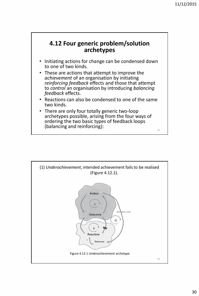
4.12 Four generic problem/solution archetypes

• Initiating actions for change can be condensed down to one of two kinds.

• These are actions that attempt to improve the achievement of an organisation by initiating reinforcing feedback effects and those that attempt to control an organisation by introducing balancing feedback effects.

• Reactions can also be condensed to one of the same two kinds.

• There are only four totally generic two-loop archetypes possible, arising from the four ways of ordering the two basic types of feedback loops (balancing and reinforcing):

59

(1) Underachievement, intended achievement fails to be realised (Figure 4.12.1).

Figure 4.12.1 Underachievement archetype

60

11/12/2015

31

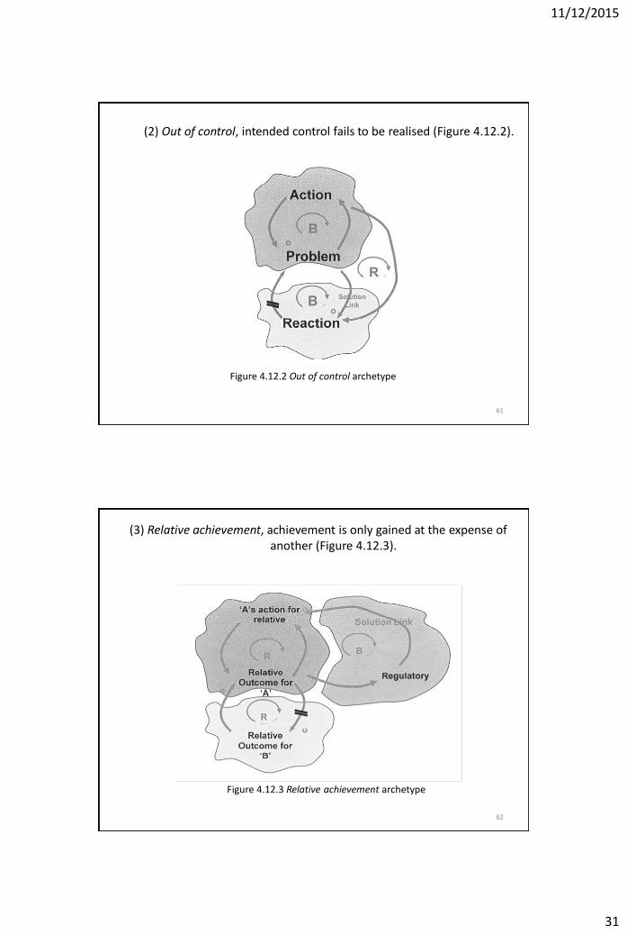
(2) Out of control, intended control fails to be realised (Figure 4.12.2).

Figure 4.12.2 Out of control archetype

61

(3) Relative achievement, achievement is only gained at the expense of another (Figure 4.12.3).

Figure 4.12.3 Relative achievement archetype

62

11/12/2015

32

(4) Relative control, control is only gained at the expense of others (Figure 4.12.4).

Figure 4.12.4 Relative control archetype

63

Semi-generic archetypes that can be mapped onto the generic underachievement archetype (Figure 4.12.1) are Limits to success, Tragedy of the commons, and Growth and underinvestment.

Semi-generic archetypes that can be mapped onto the generic out of control archetype (Figure 4.12.2) are Fixes that fail, Shifting the burden, and Accidental adversaries.

The semi-generic archetype which can be mapped onto the generic relative achievement archetype (Figure 4.12.3) is Success to the successful.

The semi-generic archetypes which can be mapped onto the generic relative control archetype (Figure 4.12.4) are Escalation and Drifting goals.

4.13 Mapping existing semi-generic problem archetypes onto four generic problem

archetypes

64

11/12/2015

33

4.14 Problem Sederhana: Tangkapan Ikan

65

66

11/12/2015

34

Tangkapan ikan

Usaha

Teknologi

+

+

Stok ikan -

+

Pertambahan Ikan alamiah

Densitas

+

+

-

+

Peningkatan usaha

+

Penghasilan

Keuntungan

Biaya +

+

+

-

+

Harga ikan

+

Harga energi

+

Lingkungan

+

Struktur fenomena penangkapan ikan

Peralatan tangkap

R1

B1 B2

R2 B3

+

67

Fish stock

Effort

Fish growth Fish catch

Change of effort

Fish growth rate

Intrinsic growth

Environtment

Fish density

Carrying capacity

(fish stock maximum)

Effect of densityRevenue

Catchability

coefficient

Profit

Cost

Cost per trip

Energy price

Price of fish

Technology

Flexibility

+

+

++

-

+

-

+

+

+

+

+

+

+++

-+

+

++

+

R1

B1

B2

R2

B3

R3

Fish stock dynamics 68

11/12/2015

35

References

1. Burger, Peter L., T. Lockman (1966), The Social Construction of Reality, Allen lane. 2. Dornbusch, Rudiger and Fischer, Stanley (1997). Mulyadi, Julius A. (Alih Bahasa). Makro-ekonomi

(Edisi Keempat). Penerbit Erlangga. 3. Duncan, Richard C. (1991), “The Life-Expectancy of Industrial Civilization”, SYSTEM DYNAMICS ’91

Proceedings of the 1991 International System Dynamics Conference, Bangkok-Thailand, August 27-30, 1991.

4. Forrester, Jay W. (1961), Industrial Dynamics, Cambridge, Mass.: MIT Press. 5. Forrester, Jay W. (1969), Urban Dynamics, Cambridge, Mass.: MIT Press. 6. Forrester, Jay W. (1971), World Dynamics, Cambridge, Mass.: Wright-Allen Press. 7. Forrester, Jay W. and Peter M. Senge (1980), “Test for Building Confidence in System Dynamics

Models”, TIMS Studies in the Management Sciences. 8. Hamilton, H.R., et al. (1969), Systems Simulation for Regional Analysis, Cambridge, Mass.: MIT

Press. 9. Kemeny, John G. (1959), A Philosopher Looks at Science, D.van Nostrand. 10. Parkin, Michael (1996). Macroeconomics (third edition). Addison - Wesley Publishing Company, Inc..

11. Popper, Karl R. (1969), Conjectures and Refutations, Routledge and Kegan Paul. 12. Richardson, G.P. & A.L. Pugh III (1981), Introduction to System Dynamics Modeling with Dynamo,

The MIT Press, Cambridge, Massachusetts. 13. Saeed, K. (1984), Policy-Modelling and the Role of the Modeller, Research Paper, Industrial

Engineering & Management Division, Asian Institute of Technology, Bangkok. 14. Sasmojo, Saswinadi (2004), Sains, Teknologi, Masyarakat dan Pembangunan, Program

Pascasarjana Studi Pembangunan ITB. 15. Senge, Peter M. (1990), The Fifth Discipline : the art and practice of the learning organization,

Doubleday/Currency, New York. 16. Sterman, John D. (1981), The Energy Transition and The Economy: A System Dynamics Approach,

PhD Thesis, Cambridge : MIT. 69

70

11/12/2015

36

71

72

11/12/2015

1

Sesi 5 Feedback Loop, Delay, dan

Nonlinearity

1

Outcomes

Pada akhir sesi peserta dapat: •mengkonsepsualisasikan sebuah fenomena

menggunakan causal loop diagram (CLD); •memahami konsep feedback loops (positif dan

negatif); •memahami konsep stock, flow, delay, dan

nonlinearity; dan •menjelaskan teori-teori yang mendasari pembuatan

CLD.

2

11/12/2015

2

5.1 Hubungan Kausal (Sebab-Akibat)

• Suatu struktur umpan –balik harus dibentuk karena adanya hubungan kausal (sebab-akibat). Dengan perkataan lain, suatu struktur umpan-balik adalah suatu causal loop (lingkar sebab-akibat).

• Struktur umpan-balik ini merupakan blok pembentuk model yang diungkapkan melalui lingkaran-lingkaran tertutup. Lingkar umpan-balik (feedback loop) tersebut menyatakan hubungan sebab-akibat variabel-variabel yang melingkar, bukan manyatakan hubungan karena adanya korelasi-korelasi statistik.

• Hubungan sebab-akibat antar sepasang variabel (variabel sebab terhadap variabel akibat), dalam suatu fenomena, harus dipandang dengan suatu konsep bahwa hubungan variabel lainnya terhadap variabel akibat dianggap tidak ada.

3

Ada 2 macam hubungan kausal, yaitu: • hubungan kausal positif; dan • hubungan kausal negatif. Ada 2 macam lingkar umpan-balik, yaitu: • lingkar umpan-balik positif (growth);dan • lingkar umpan –balik negatif (goal seeking).

Sedangkan suatu korelasi statistik antara sepasang variabel, dalam suatu fenomena, diturunkan dari data kedua variabel tersebut yang diperoleh dalam keadaan (kondisi) semua variabel yang terdapat dalam fenomena itu berhubungan satu dengan yang lainnya dan kesemuanya berubah secara simultan.

4

11/12/2015

3

5

6

11/12/2015

4

Causal-loop diagram (CLD)

Populasi Kelahiran Kematian

+

- +

(+) (-)

+

7

5.2 Level (Stock) dan Rate (Flow)

• Dalam merepresentasikan aktivitas dalam suatu lingkar umpan-balik, digunakan dua jenis variabel yang disebut sebagai level dan rate.

• Level menyatakan kondisi sistem pada setiap saat. Dalam kerekayasaan (engineering) level sistem lebih dikenal sebagai state variable system. Level merupakan akumulasi di dalam sistem.

• Persamaan suatu variabel rate merupakan suatu struktur kebijakan (policy) yang menjelaskan mengapa dan bagaimana suatu keputusan (action) dibuat berdasarkan kepada informasi yang tersedia di dalam sistem. Rate inilah satu-satunya variabel dalam model yang dapat mempengaruhi level.

(rate disebut juga sebagai decision point)

8

11/12/2015

5

Level (Stock) and Rate (Flow)

• Levels and rates as loop sub-substructure A feedback loop consists of two distinctly different types of variables, the levels (states) and the rates (actions). Except for constants, these two are sufficient for represent a feedback loop. Both are necessary.

• Levels are integrations The level integrate (or accumulate) the result of action in a system. The level variables can not change instantaneously.

• Level are changed only by the rates A level variable is computed by the change, due the rate variables, that alters the previous value of the level. The earlier value of the level is carried forward from the previous period. It’s altered by rates that flow over the intervening time interval. The present value of a level variable can be computed without the present or previous values of any other level variables.

• Levels and rates not distinguised by units of measure The units of measure of a variable do not distinguish between a level and a rate. The identification must recognize the difference between a variable created by integration and one that is a policy statement in the system. 9

Level (Stock) and Rate (Flow)

• Rates not instantaneously measurable No rate of flow can be measured except as an average over a period of time. No rate can, in priciple, control another rate without an intervening level variable.

• Rates dapend only on levels and constants No rate variable depends directly on any other rate variable. The rate equations (policy statements) of system are of simple algebraic form; they don’t involve time or the solution interval; they are not dependent on their own past value.

• Level variables and rate variables must alternate Any path through the structure of a system encounters alternating level and rate variables.

• Levels completely describe the system condition Only the values of the level variables are needed to fully describe the condition of a system. Rate variables are not needed because they can be computed from the levels.

10

11/12/2015

6

5.3 Delay

11

[nonlinier]

5.4 Nonlinearity

12

11/12/2015

1

Sesi 6 Simulation Software:

Powersim Studio

1

Outcomes

At the end of this session, participants will be able to:

• construct flow diagram based on a CLD

• simulate the model using Powersim Studio software (Saving Model).

2

11/12/2015

2

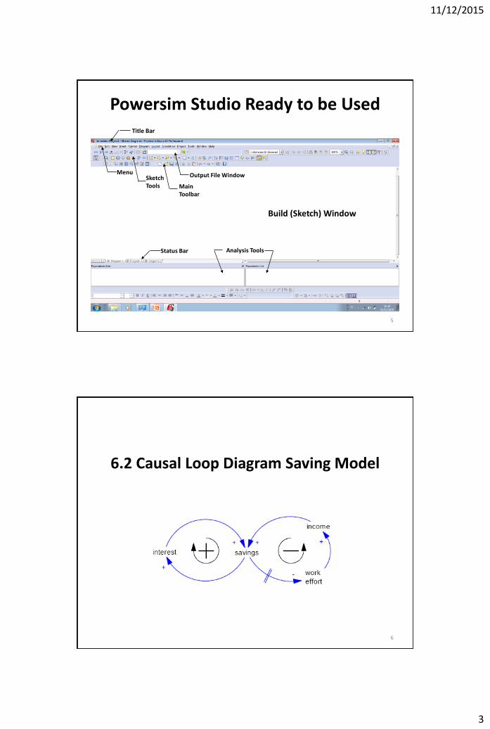
6.1 Powersim Studio Windows

3

Document Tools, contain of component and

format for documentation, view , tools and

help

Modeling Tools, contain of button for

building stock and flow diagram and view

the simulation results

Diagram Tools, contaiin of

model sheet diagram

Diagram View, tp place for building

the models

Powersim Studio General View

11/12/2015

3

Powersim Studio Ready to be Used

5

Analysis Tools Status Bar

Sketch Tools Main

Toolbar

Menu

Title Bar

Output File Window

Build (Sketch) Window

6.2 Causal Loop Diagram Saving Model

6

11/12/2015

4

6.3 Model Building Step 1

1. Open Powersim Studio, and click “New Model” in Main Toolbar.

2. Click next button in the new project wizard window

7

Step 2

3. Choose the language, then click next

8

11/12/2015

5

Step 3

4. Choose Studio 10 file format, then click next

9

Step 4

5. Choose Enforce Time Unit Consistency, then click next

10

11/12/2015

6

Step 5

6. Choose calendar interdependent simulation, then choose next

11

Step 6

7. Choose use as default in all new projects, then click next

12

11/12/2015

7

Step 7

8. Choose Use as default in all projects, then click next

13

Step 8 9. Choose time step 0.25, then click next

14

11/12/2015

8

Step 9

10. Click Finish, so ready to build model flow diagram

15

Step 10 11. Ready to Build Saving Model Flow Diagram

16

11/12/2015

9

6.4 Building Saving Model • Sketch tools

• Activate tools for creating a level from sketch tools, than put in the sketch window or diagram view,

• Type the name of the level Saving in editing box, then enter,

• Activate tools for creating a Flow with Rate,

• than connect it to the “saving” level and naming it Interest,

• Activate tools for creating a Constant and naming it Interest Rate,

• Activate tools for creating a Link and link the savang level and Interest Rate constant to the Interest auxilary,

17

6.5 Inputting Model Equations (1)

• Double click the Saving level • input 100000 in definition windows • input rupiah for the unit measure • Click apply, then ok

• If rupiah not yet defined this message will appear, and click yes

• click next, then apply and finish

18

11/12/2015

10

6.5 Inputting Model Equations (2) Double click the Interest Rate constant • input 0.05 in definition windows • input 1/year for the unit measure • Click apply, then ok

19

• Double click Interest auxiliary • input equation Interest Rate*Saving • Activate unit measure v • Click apply, then ok

Saving Model Flow Diagram

• Saving Model ready to be simulated

20

11/12/2015

11

6.6 Model Simulation (1)

21

• Activate tool for creating a Time Graph for simulating the saving and interest behavior.

• Activate tool for creating a Time Table for simulating the saving and interest behavior.

6.6 Model Simulation (2)

22

• Drag Saving level to the Time Graph and the Time Table

• Drag Interest rate to the Time Graph and the Time Table

• Click the simulation button to run the Saving Model simulation

0 20 40 60 80 1000

5,000,000

10,000,000

15,000,000

rupiah

Saving

0 20 40 60 80 100

0

200,000

400,000

600,000

rupiah/year

Interest

year Saving (rupiah)

0

20

40

60

80

100

100,000.00

270,148.49

729,802.09

1,971,549.35

5,326,110.88

14,388,408.35

year Interest (rupiah/year)

0

20

40

60

80

100

5,000.00

13,507.42

36,490.10

98,577.47

266,305.54

719,420.42

Saving

Interest

Interest Rate

11/12/2015

12

23

24

12/11/2015

1

Sesi 7 Latihan Simulasi

1

Outcomes

At the end of this session, participants will be able to:

• Develop Stock and flow diagram based on Causal Loop Diagram;

• Simulate the Model Using Powersim Studio (positive feedback, negative feedback, non linearity, Population model, investment model, and inventory model).

2

12/11/2015

2

7.1 Positive Model (Population)

3

Causal Loop Diagram Population

Population

Population Growth

Population Growth Fraction

+

+

+

+

4

12/11/2015

3

Population Model

5

Level_1

Rate_1

Constant_1

Population Model

6

12/11/2015

4

Population Model Behaviour

7

7.2 Negative Feedback (Investment Model)

8

12/11/2015

5

Causal Loop Diagram Investment Model

Capital Investment

Desired Capital

Time to Adjust Capital

- -

+

+ -

9

Investment Model

10

12/11/2015

6

Investment Model Behaviour

11

NEGATIVE FEEDBACK AND GOAL SEEKING

Kapital

Investment

Time to adjustkapital Desired Kapital

0 10 20 30 40 50

2.000

4.000

6.000

8.000

Million_Dollars

Kapital

Desired Kapital

0 10 20 30 40 500

500

1.000

1.500

Million_Dollars/year

In

ve

stm

en

t

7.3 Positive and Negative Feeback

(Population Model)

12

12/11/2015

7

Causal Loop Diagram Population Model

Population

Birth Rate

Fertility

+

+

+ +

Death Rate

- +

-

Mortality

+

13

14

Population Model

12/11/2015

8

Population Model Behaviour

15

7.4 Delay

(Employee Model)

16

12/11/2015

9

Pegawai PensiunPengangkatan

Pegawai

Pertambahan Pegawai

dari Kebutuhan

Pegawai yang

Dibutuhkan

+

-

+

-

+

+

-

-

• CLD Without Delay

17

Pegawai PensiunPengangkatan

Pegawai

Pertambahan Pegawai

dari Kebutuhan

Pegawai yang

Dibutuhkan

+

-

+

-

+

+

-

Pertambahan

Pegawai dari Pensiun

Pensiun Rata-Rata

+

+

+

-

+

• CLD Dengan Delay

18

12/11/2015

10

• Non-Delay Employee Model

19

• Non-Delay Employee Model Behaviour

20

MODEL TANPA DELAY

Jumlah Pegawai

PensiunPengangkatan

Masa kerja

Pegawaidibutuhkan

Pertambahanpegawai ygdibutuhkan

Waktupengangkatan

0 5 10 15 20 251.000

2.000

3.000

4.000

5.000

6.000

7.000

jiwa

Jumlah Pegawai

Pegawai dibutuhkan

12/11/2015

11

• Delayed Employee Mode Behaviour

21

MODEL DENGAN DELAY

Jumlah Pegawai 2

Pensiun 2Pengangkatan 2

Masa kerja 2

Pegawaidibutuhkan 2

Pertambahanpegawai yg

dibutuhkan 2

Waktupengangkatan 2

Pensiun rata-rata 2

Waktu meratakanpensiun 2

Pertambahanpegawai dari

pensiun 2

0 5 10 15 20 25

1.000

2.000

3.000

4.000

5.000

6.000

7.000

jiwa

Jumlah Pegawai 2

Pegawai dibutuhkan 2

0 5 10 15 20 25

500

1.000

1.500

2.000

jiwa/year

Pe

ng

an

gk

ata

n 2

7.5 Nonlinearity

(Pollution Model)

22

12/11/2015

12

• Linear CLD

PollutionPollution

Absorption Rate

Pollution Growth

Rate

++

-

Pollution

Absorption Time

-

-

23

• Non-Linear CLD

24

PollutionPollution

Absorption Rate

Pollution Growth

Rate

++

-

Pollution

Absorption Time

-

-

Pollution Ratio

+

+

+

12/11/2015

13

• Linear Pollution Model

25

0 2 4 6 8 10

0

5

10

15

20

Ton_CO2

Po

llu

tio

n

Pollution

Pollution growth Pollution absorptionrate

Pollution absortiontimePollution growth

rate constant

0 20 40 60 80 100

0

100

200

300

400

500

600

700

800

Ton_CO2

Po

llu

tio

n

• Non Linear Model

26

Pollution

Pollution growth Pollution absorptionrate

Pollution growthrate

Pollution Standar

Pollution ration Pollution AbsortionTime

12/11/2015

14

7.6 Investment Model

27

Causal Loop Diagram Investment

Capital

Investment

Desired Capital

+

+

-

+

Depreciation

- + -

Life of capital

-

Income

Smoothed Income

Consumption

Gov Spending

Propensity to Consume

Time to Smooth Income

KOR

Normal Time to Adjust Capital

+ +

+ +

-

+

+ +

+

-

+

-

+ + //

28

12/11/2015

15

Causal Loop Diagram Investment Model

CapitalInvestment Depreciation

Life of Capital

Desired Capital

Income

Smoothed Income

Gov Spending

Consumption

Propensity to

Consume

Time to Smooth

Income

KOR

Normal Time to

Adjust Capital

+

-

+

--

-

+

+

-

+

+

+

+

++

+

+

+

- -

+

29

Investment Model

30

Capital

Investment Depreciation

Life of capital

GovernmentExpenditure

Change in GE

GE Trend

Income

Smoothed income

Time to smoothedincome

Consumption

Prospensity toconsume

Iinitial GE

Desired Kapital

Capital Output Ratio-KOR

Normal Time toAdjust Kapital-NTAK

Initial SmoothedIncome

12/11/2015

16

Investment Model Behaviour (Equilibrium)

31

0 20 40 60 80 100

0

500

1.000

Million_Dollars/years

Government Expenditure

Consumption

Income

Investment

Investment Model Behaviour (GE Growth 1 %/year)

32

0 20 40 60 80 100

0

500

1.000

1.500

2.000

2.500

Million_Dollars/years

Government Expenditure

Consumption

Income

Investment

12/11/2015

17

7.7 Model Inventory

33

ABC Manufacturing Inventory (1) SCENARIO • ABC Manufacturing would like to use simulation to better

understand the interaction between the amounts of merchandise the public orders and their own inventory and production levels.

• Since the company often experiences oscillations in their inventory and production levels, they think the first step in solving this problem is to build a model that would explain the relevant interactions.

• They know that their production policy concists of two components increasing or decreasing the inventory to match an optimal or desired level of inventory and keeping inventory high enough to cover what they expect their demand will be in the future.

• To be safe, they like to keep four times as much inventory on hand as they think will be needed to cover demand.

• In addition, production is set so that one-sixth of the discrepancy between the desired and actual inventory is corrected every week.

34

12/11/2015

18

ABC Manufacturing Inventory (2)

• Their assumptions about future demand are based on the current order rate.

• The current order rate constitutes the real demand that the company faces.

• Their policy formulating their expected demand is simple.

• They want to correct one-eighth of the difference between their real and expected demands every week.

• When their beliefs about future demand change, this affects their desired level of inventory and the rate at which they produce widgets, according to the production policy described above.

•

35

ABC Manufacturing Inventory (3)

• When widgets are produced, they go straight to warehouse to be stored as inventory.

• No Product can go from the production line straight to the customer; it must go into the inventory first.

• Shipments are made only from inventory. Because the company keeps four times as much inventory as they think they will need at any time, they believe they are able to ship the necessary products to fulfill every order.

• Therefore, they are not now concerned with backlogs and their effects (although a negative inventory while meaningless in reality, can here be constructed to represent a backlog).

36

12/11/2015

19

CLD Inventory Model

Inventory

Production

Desired Inventory

Expected Demand

Inventory Coverage

Order Rate

Time to Correct Inventory

Change in Expected Demand

Time to Change Expectations

+

+

+

+

-

-

+

+

+

-

-

- +

Shipment

-

- -

-

37

Powersim Studio

38

12/11/2015

20

Setting The Simulation Time (1)

39

Setting The Simulation Time (2)

40

12/11/2015

21

Model Building (1)

41

Model Building (2)

42

12/11/2015

22

Model Building (3)

43

Model Building (4)

44

12/11/2015

23

Model Building (5)

45

Model Building (6)

46

12/11/2015

24

Model Building (7)

47

Model Building (8)

48

12/11/2015

25

Model Building (9)

49

Model Building (10)

50

12/11/2015

26

Model Building (11)

51

Model Building (12)

By click right mouse

52

12/11/2015

27

Model Building (13)

;

53

Model Building (14)

54

12/11/2015

28

Model Building (15)

55

Model Building (16)

56

12/11/2015

29

Model Building (17)

57

Model Building (18)

58

12/11/2015

30

Model Building (19)

59

Model Building (20)

60

12/11/2015

31

Model Building (21)

61

Model Building (22)

62

12/11/2015

32

Model Building (23)

63

Model Building (24)

64

12/11/2015

33

Model Building (25)

65

Model Building (26)

66

12/11/2015

34

Model Building (27)

67

Model Behavior (1)

68

12/11/2015

35

Model Behavior (2)

69

Model Behavior (3)

70

12/11/2015

36

Model Behavior (4)

71

Model Behavior (5)

72

12/11/2015

37

Conclusion

• The purpose of this session was to ilustrate how to build a simple model in Powersim Studio. Although the model is simple, it shows how to use Studio to create simulation models, and gives you a brief introduction to the technical aspect of modelling using the software.

• We recommend you to take a closer look at some of the other tutorials as well, and also to study the sample models. These shows various business cases as well as features in Studio. We would also encourage you to refer to Help for Studio, where you can find answers to a wide range of questions.

73

74

12/11/2015

38

75

76

12/11/2015

1

Sesi 8 Model Ketersediaan (Availability)

1

Outcomes

At the end of this session, participants will be able to:

• understand some concepts of availability that are widely used in modeling using the system dynamics approach;

• understand the differences among the availability concepts; and

• build a model based on each of availability concepts using Powersim Studio software.

2

12/11/2015

2

Simulation Objectives

• Participants are able to understand the concept of availability that was widely used in modeling using the system dynamics approach.

• Participants are able to build a model that is based on each of availability concepts using the software Powersim Studio.

• Participants are able to understand the differences among the availability concepts.

3

8.1 Availability Concept

• Availability of a resource means a resource that is committable, operable, or usable upon demand to perform its designated or required.

• If Availability >= 1, means available;

if Availability < 1 means not available

• Availability concept (cash) – Cash Availability = Cash Adequacy Time /Targeted Cash

Adequacy Time

– Cash Availability = Cash/Desired Cash

– Cash Availability = Maximum Outcome/Desired Outcome

– Implicit Cash Availability;

Maximum Outcome = Cash/Targeted Cash Adequacy Time

4

12/11/2015

3

Availability Concept 1

5

Availability Concept 1

Cash Availability = Cash Adequacy Time / Targeted Cash Adequacy Time

Note: Can not be used when the desired expenditure is zero

Cash 1

Income 1 Expenditure 1

Cash AdequacyTime 1

Cash Availability 1

Targeted CashAdequacy Time 1

Desired Expenditure1

Cash AvailabilityEffect 1

Availability Concept 2

6

Availability Concept 2

Cash Availability = Cash / Desired Cash

Note: Can not be used when the desired expenditure is zero

Cash 2

Income 2 Expenditure 2

Desired Cash 2

Cash Availability 2

Targeted CashAdequacy Time 2

Desired Expenditure2

Cash AvailabilityEffect 2

12/11/2015

4

Availability Concept 3

7

Availability Concept 3

Cash Availability = Maximum Expenditure / Desired Expenditure

Note: Can not be used when the desired expenditure is zero

Cash 3

Income 3 Expenditure 3

MaximumExpenditure 3

Cash Availability 3

Targeted CashAdequacy Time 3

Desired Expenditure3

Cash AvailabilityEffect 3

Availability Concept 4

8

Availability Concept 4

(Implicit Cash Availability) Masimum Expenditure = Cash / Targeted Cash AdequacyTime

Note: Can be used when the desired expenditure is zero

Cash 4

Income 4 EXpenditure 4

Max Expenditure 4

Targeted CashAdequacy Time 4

Desired Expenditure4

12/11/2015

5

8.2 Simulation Results

• Although it is using the four different model structures but will produce the same dynamic behavior.

9

0 5 10

0,0

0,5

1,0

1,5

2,0

Cash Availability 1

Cash Availability 2

Cash Availability 3

0 5 10

1.999.999,0

1.999.999,5

2.000.000,0

2.000.000,5

2.000.001,0

rupiah

Cash 1

Cash 2

Cash 3

Cash 4

0 5 10

999.999,0

999.999,5

1.000.000,0

1.000.000,5

1.000.001,0

rupiah/year

Income 1

Expenditure 1

Income 2

Expenditure 2

Income 3

Expenditure 3

Income 4

EXpenditure 4

Ina Juniarti +628164210120 10

12/11/2015

6

Ina Juniarti +628164210120 11

Ina Juniarti +628164210120 12