Unsupervised Regression with Applications toNonlinear System Identification

Ali RahimiIntel Research Seattle

Seattle, WA 98105ali.rahimi@intel.com

Ben RechtCalifornia Institute of Technology

Pasadena, CA 91125brecht@ist.caltech.edu

Abstract

We derive a cost functional for estimating the relationship between high-dimensional observations and the low-dimensional process that generated themwith no input-output examples. Limiting our search to invertible observationfunctions confers numerous benefits, including a compact representation and nosuboptimal local minima. Our approximation algorithms for optimizing this costfunctional are fast and give diagnostic bounds on the quality of their solution. Ourmethod can be viewed as a manifold learning algorithm that utilizes a prior on thelow-dimensional manifold coordinates. The benefits of taking advantage of suchpriors in manifold learning and searching for the inverse observation functionsin system identification are demonstrated empirically by learning to track mov-ing targets from raw measurements in a sensor network setting and in an RFIDtracking experiment.

1 Introduction

Measurements from sensor systems typically serve as a proxy for latent variables of interest. Torecover these latent variables, the parameters of the sensor system must first be determined. Whenpairs of measurements and their corresponding latent variables are available, fully supervised re-gression techniques may be applied to learn a mapping between latent states and measurements.In many applications, however, latent states cannot be observed and only a diffuse prior on them isavailable. In such cases, marginalizing over the latent variables and searching for the model parame-ters using Expectation Maximization (EM) has become a popular approach [3,9,19]. Unfortunately,such algorithms are prone to local minima and require very careful initialization in practice.

Using a simple change-of-variable model, we derive an approximation algorithm for the Unsuper-vised Regression problem – estimating the nonlinear relationship between latent-states and theirobservations when no example pairs are available, when the observation function is invertible, andwhen the measurement noise is small. Our method is not susceptible to local minima and provides aguarantee on the quality of the recovered observation function. We identify conditions under whichour estimate of the mapping is asymptotically consistent and empirically evaluate the quality of oursolutions and their stability under variations of the prior. Because our algorithm takes advantage ofan explicit prior on the latent variables, it recovers latent variables more accurately than manifoldlearning algorithms when applied to similar tasks.

Our method may be applied to estimate the observation function in nonlinear dynamical systemsby enforcing a Markovian dynamics prior over the latent states. We demonstrate this approachto nonlinear system identification by learning to track a moving object in a field of completelyuncalibrated sensor nodes whose measurement functions are unknown. Given that the object movessmoothly over time, our algorithm learns a function that maps the raw measurements from the sensornetwork to the target’s location. In another experiment, we learn to track Radio Frequency ID (RFID)

tags given a sequence of voltage measurements induced by the tag in a set of antennae . Given onlythese measurements and that the tag moves smoothly over time, we can recover a mapping fromthe voltages to the position of the tag. These results are surprising because no parametric sensormodel is available in either scenario. We are able to recover the measurement model up to an affinetransform given only raw measurement sequences and a diffuse prior on the state sequence.

2 A diffeomorphic warping model for unsupervised regression

We assume that the set X = xi1···N of latent variables is drawn (not necessarily iid) from a knowndistribution, pX(X) = pX(x1, · · · , xN ). The set of measurements Y = yi1···N is the output ofan unknown invertible nonlinearity applied to each latent variable, yi = f0(xi). We assume thatobservations, yi ∈ RD, are higher dimensional than latent variables xi ∈ Rd. Computing a MAPestimate of f0 requires marginalizing over X and maximizing over f . EM, or some other form ofcoordinate ascent on a Jensen bound of the likelihood, is a common way of estimating the parametersof this model, but such methods suffer from local minima.

Because we have assumed that f0 is invertible and that there is no observation noise, this processdescribes a change of variables. The true distribution pY(Y) over Y can be computed in closed formusing a generalization of the standard change of variables formula (see [14, thm 9.3.1] and [7, chap11]):

pY(Y) = pY(Y; f0) = pX(f−10 (y1), · · · , f−1

0 (yN ))N∏

i=1

det(∇f

(f−10 (yi)

)′∇f(f−10 (yi)

) )− 12

.

(1)The determinant corrects the warping of each infinitesimal volume element around f−1

0 (yi) by ac-counting for the stretching induced by the nonlinearity. The change of variables formula immedi-ately yields a likelihood over f , circumventing the need for integrating over the latent variables.

We assume f0 diffeomorphically maps a ball in Rd containing the data onto its image. In this case,there exists a function g defined on an open set containing the image of f such that g(f(x)) = xand ∇g∇f = I for all x in the open set [5]. Consequently, we can substitute g for f−1 in (1) and,taking advantage of the identity det(∇f ′∇f)−1 = det∇g∇g′, write its log likelihood as

lY(Y; g) = log pY(Y; g) = log pX(g(y1), . . . , g(yN )) +12

N∑i=1

log det (∇g(yi)∇g(yi)′) . (2)

For many common priors pX, the maximum likelihood g yields an asymptotically consistent es-timate of the true distribution pY. When certain conditions on pX are met (including stationarity,ergodicity, and kth-order Markov approximability), a generalized version of the Shannon-McMillan-Breiman theorem [1] guarantees that log pY(Y; g) asymptotically converges to the relative entropyrate between the true pY(Y) and pY(Y; g). This quantity is maximized when these two distribu-tions are equal. Therefore, if the true pY follows the change of variable model (1), the recovered gconverges to the true f−1

0 in the sense that they both describe a change of variable from the priordistribution pX to the distribution pY.

Note that although our generative model assumes no observation noise, some noise in Y can betolerated if we constrain our search over smooth functions g. This way, small perturbations in y dueto observation noise produce small perturbations in g(y).

3 Approximation algorithms for finding the inverse mapping

We constrain our search for g to a subset of smooth functions by requiring that g have a finiterepresentation as a weighted sum of positive definite kernels k centered on observed data, g(y) =∑N

i=1 cik(y, yi), with the weight vectors ci ∈ Rd. Accordingly, applying g to the set of observationsgives g(Y) = CK, where C = [ c1···cN ] and K is the kernel matrix with Kij = k(yi, yj). Inaddition, ∇g(y) = C∆(y), where ∆(y) is an N × D matrix whose ith row is ∂k(yi,y)

∂y . We tunethe smoothness of g by regularizing (2) with the RKHS norm [17] of g. This norm has the form‖g‖2

k = trCKC′, and the regularization parameter is set to λ2 .

For simplicity, we require pX to be a Gaussian with mean zero and inverse covariance ΩX, but wenote our methods can be extended to any log-concave distribution. Substituting into (2) and addingthe smoothness penalty on g, we obtain:

maxC

−vec (KC′)′ ΩXvec (KC′)− λtrCKC′ +N∑

i=1

log detC∆(yi)∆(yi)′C′, (3)

where the vec (·) operator stacks up the columns of its matrix argument into a column vector.

Equation (3) is not concave in C and is likely to be hard to maximize exactly. This is becauselog det(A′A) is not concave for A ∈ Rd×D. Since the cost is non-concave, gradient descentmethods may converge to local minima. Such local minima, in addition to the burdensome time andstorage requirements, rule out descent strategies for optimizing (3).

Our first algorithm for approximately solving this optimization problem constructs a semidefiniterelaxation using a standard approach that replaces outer products of vectors with positive definitematrices. Rewrite (3) as

maxC

− tr(Mvec (C′) vec (C′)′

)+

N∑i=1

log det([

trJkli vec (C′) vec (C′)′

])(4)

M = (Id ⊗K)ΩX(Id ⊗K) + λ(Id ⊗K) , Jkli = Elk ⊗∆(yi)∆(yi)′ (5)

where the klth entry of the matrix argument of the logdet is as specified, and the matrix Eij is zeroeverywhere except for 1 in its ijth entry. This optimization is equivalent to

maxZ0

− tr (MZ) +N∑

i=1

log det([

trJkli Z

]), (6)

subject to the additional constraint that rank(Z) = 1. Dropping the rank constraint yields a concaverelaxation for (3). Standard interior point methods [20] or subgradient methods [2] can efficientlycompute the optimal Z for this relaxed problem. A set of coefficients C can then be extracted fromthe top eigenvectors of the optimal Z, yielding an approximate solution to (3). Since (6) withoutthe rank constraint is a relaxation of (3), the optimum of (6) is an upper bound on that of (3). Thuswe can bound the difference in the value of the extracted solution and that of the global maximumof (3). As we will see in the following section, this method produces high quality solutions for adiverse set of learning problems.

In practice, standard algorithms for (6) run slowly for large data sets, so we have developed anintuitive algorithm that also provides good approximations and runs much more quickly. The non-concave logdet term serves to prevent the optimal solution of (2) from collapsing to g(y) = 0,since X = 0 is the most likely setting for the zero-mean Gaussian prior pX. To circumvent thenon-concavity of the logdet term, we replace it with constraints requiring that the sample mean andcovariance of g(Y) match the expected mean and covariance of the random variables X. Thesemoment constraints prevent the optimal solution from collapsing to zero while remaining in thetypical set of pX. The expected covariance of X, denoted by ΛX, can be computed by averagingthe block diagonals of Ω−1

X . However, the particular choice of ΛX only influences the final solutionup to a scaling and rotation on g, so in practice, we set it to the identity matrix. We thus obtain thefollowing optimization problem:

minC

vec (KC′)′ ΩXvec (KC′) + λtrCKC′ (7)

s.t.1N

CK(CK)′ = ΛX (8)

1N

CK1 = 0, (9)

where 1 is a column vector of 1s. This optimization problem searches for a g that transformsobservations into variables that are given high probability by pX and match its stationary statistics.This is a quadratic minimization with a single quadratic constraint and, after eliminating the linearconstraints with a change of variables, can be solved as a generalized eigenvalue problem [4].

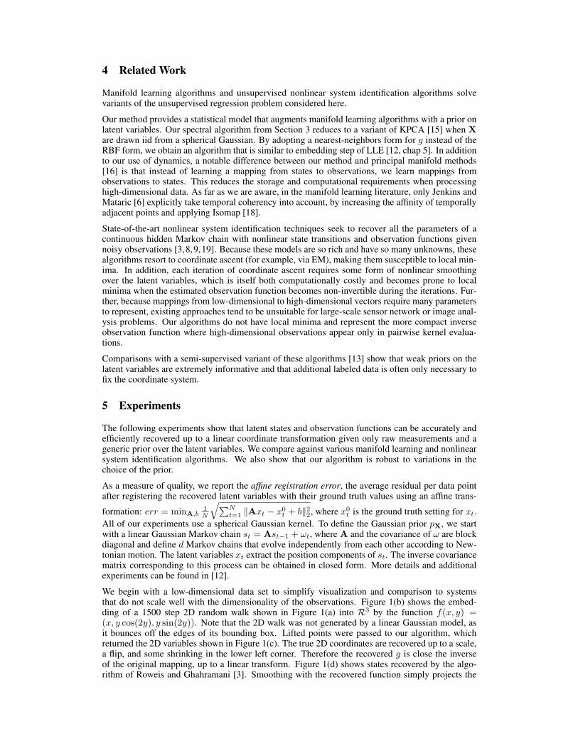
4 Related Work

Manifold learning algorithms and unsupervised nonlinear system identification algorithms solvevariants of the unsupervised regression problem considered here.

Our method provides a statistical model that augments manifold learning algorithms with a prior onlatent variables. Our spectral algorithm from Section 3 reduces to a variant of KPCA [15] when Xare drawn iid from a spherical Gaussian. By adopting a nearest-neighbors form for g instead of theRBF form, we obtain an algorithm that is similar to embedding step of LLE [12, chap 5]. In additionto our use of dynamics, a notable difference between our method and principal manifold methods[16] is that instead of learning a mapping from states to observations, we learn mappings fromobservations to states. This reduces the storage and computational requirements when processinghigh-dimensional data. As far as we are aware, in the manifold learning literature, only Jenkins andMataric [6] explicitly take temporal coherency into account, by increasing the affinity of temporallyadjacent points and applying Isomap [18].

State-of-the-art nonlinear system identification techniques seek to recover all the parameters of acontinuous hidden Markov chain with nonlinear state transitions and observation functions givennoisy observations [3,8,9,19]. Because these models are so rich and have so many unknowns, thesealgorithms resort to coordinate ascent (for example, via EM), making them susceptible to local min-ima. In addition, each iteration of coordinate ascent requires some form of nonlinear smoothingover the latent variables, which is itself both computationally costly and becomes prone to localminima when the estimated observation function becomes non-invertible during the iterations. Fur-ther, because mappings from low-dimensional to high-dimensional vectors require many parametersto represent, existing approaches tend to be unsuitable for large-scale sensor network or image anal-ysis problems. Our algorithms do not have local minima and represent the more compact inverseobservation function where high-dimensional observations appear only in pairwise kernel evalua-tions.

Comparisons with a semi-supervised variant of these algorithms [13] show that weak priors on thelatent variables are extremely informative and that additional labeled data is often only necessary tofix the coordinate system.

5 Experiments

The following experiments show that latent states and observation functions can be accurately andefficiently recovered up to a linear coordinate transformation given only raw measurements and ageneric prior over the latent variables. We compare against various manifold learning and nonlinearsystem identification algorithms. We also show that our algorithm is robust to variations in thechoice of the prior.

As a measure of quality, we report the affine registration error, the average residual per data pointafter registering the recovered latent variables with their ground truth values using an affine trans-

formation: err = minA,b1N

√∑Nt=1 ‖Axt − x0

t + b‖22, where x0

t is the ground truth setting for xt.All of our experiments use a spherical Gaussian kernel. To define the Gaussian prior pX, we startwith a linear Gaussian Markov chain st = Ast−1 + ωt, where A and the covariance of ω are blockdiagonal and define d Markov chains that evolve independently from each other according to New-tonian motion. The latent variables xt extract the position components of st. The inverse covariancematrix corresponding to this process can be obtained in closed form. More details and additionalexperiments can be found in [12].

We begin with a low-dimensional data set to simplify visualization and comparison to systemsthat do not scale well with the dimensionality of the observations. Figure 1(b) shows the embed-ding of a 1500 step 2D random walk shown in Figure 1(a) into R3 by the function f(x, y) =(x, y cos(2y), y sin(2y)). Note that the 2D walk was not generated by a linear Gaussian model, asit bounces off the edges of its bounding box. Lifted points were passed to our algorithm, whichreturned the 2D variables shown in Figure 1(c). The true 2D coordinates are recovered up to a scale,a flip, and some shrinking in the lower left corner. Therefore the recovered g is close the inverseof the original mapping, up to a linear transform. Figure 1(d) shows states recovered by the algo-rithm of Roweis and Ghahramani [3]. Smoothing with the recovered function simply projects the

(a) (b) 02

46

−50

5−6

−5

−4

−3

−2

−1

0

1

2

3

4

(c)

(d) (e) (f)

Figure 1: (a) 2D ground truth trajectory. Brighter colors indicate greater distance to the origin. (b) Embeddingof the trajectory intoR3. (c) Latent variables are recovered up to a linear transformation and minor distortion.Roweis-Ghahramani (d), Isomap (e), and Isomap+temporal coherence (f) recovered low-dimensional coordi-nates that exhibit folding and other artifacts that cannot be corrected by a linear transformation.

observations without unrolling the roll. The joint-max version of this algorithm took about an hourto converge on a 1Ghz Pentium III and converges only when started at solutions that are sufficientlyclose to the true solution. Our spectral algorithm took about 10 seconds. Isomap (Figure 1(e)) per-forms poorly on this data set due to the low sampling rate on the manifold and the fact that the truemapping f is not isometric. Including temporal neighbors into Isomap’s neighborhood structure (asper ST-Isomap) creates some folding, and the true underlying walk is not recovered (Figure 1(f)).KPCA (not shown) chooses a linear projection that simply eliminates the first coordinate. We foundthe optimal parameter settings for Isomap, KPCA, and ST-Isomap by a fine grid search over theparameter space of each algorithm.

The upper bound on the log-likelihood returned by the relaxation (6) serves as a diagnostic on thequality of our approximations. This bound was −3.9 × 10−3 for this experiment. Rounding theresult of the relaxation returned a g with log likelihood −5.5 × 10−3. The spectral approximation(7) also returned a solution with log likelihood −5.5 × 10−3, confirming our experience that thesealgorithms usually return similar solutions. For comparison, log-likelihood of KPCA’s solution was−1.69× 10−2, significantly less likely than our solutions, or the upper bound.

5.1 Learning to track in an uncalibrated sensor network

We consider an artificial distributed sensor network scenario where many sensor nodes are deployedrandomly in a field in order to track a moving target (Figure 2(a)). The location of the sensornodes is unknown, and the sensors are uncalibrated, so that it is not known how the position of thetarget maps to the reported measurements. This situation arises when it is not feasible to calibrateeach sensor prior to deployment or when variations in environmental conditions affect each sensordifferently. Given only the raw measurements produced by the network from watching a smoothlymoving target, we wish to learn a mapping from these measurements to the location of the target,even though no functional form for the measurement model is available. A similar problem wasconsidered by [11], who sought to recover the location of sensor nodes using off-the-shelf manifoldlearning algorithms.

Each latent state xt is the unknown position of the target at time t. The unknown function f(xt)gives the set of measurements yt reported by the sensor network at time t. Figure 2(b) shows thetime series of measurements from observing the target. In this case, measurements were generatedby having each sensor s report its true distance ds

t to the target at time t and passing it through arandom nonlinearity of the form αs exp(−βsds

t ). Note that only f , not the measurement functionof each sensor, needs be invertible. This is equivalent to requiring that a memoryless mapping frommeasurements to positions must exist.

(a) −1 −0.8 −0.6 −0.4 −0.2 0 0.2 0.4 0.6 0.8 1−1

−0.8

−0.6

−0.4

−0.2

0

0.2

0.4

0.6

0.8

1

(b) 1000 1010 1020 1030 1040 1050 1060 1070 1080 1090 11000

0.5

1

1.5

2

2.5

(c) −0.03 −0.02 −0.01 0 0.01 0.02 0.03 0.04 0.05

−0.04

−0.03

−0.02

−0.01

0

0.01

0.02

0.03

0.04

(d) −1 −0.8 −0.6 −0.4 −0.2 0 0.2 0.4 0.6 0.8 1−1

−0.8

−0.6

−0.4

−0.2

0

0.2

0.4

0.6

0.8

1

(e) 0.007 0.008 0.009 0.01 0.011 0.012 0.013 0.014 0.015 0.016−14

−13

−12

−11

−10

−9

−8

−7

−6

−5

−4x 10−3

(f)−0.027 −0.0265 −0.026 −0.0255 −0.025 −0.0245 −0.024 −0.0235 −0.023−9

−8

−7

−6

−5

−4

−3

−2

−1

0x 10−3

Figure 2: (a) A target followed a smooth trajectory (dotted line) in a field of 100 randomly placed uncalibratedsensors with random and unknown observation functions (circle). (b) Time series of measurements producedby the sensor network in response to the target’s motion. (c) The recovered trajectory given only raw sensormeasurements, and no information about the observation function (other than smoothness and invertibility). Itis recovered up to scaling and a rotation. (d) To test the recovered mapping further, the target was made tofollow a zigzag pattern. (e) Output of g on the resulting measurements. The resulting trajectory is again similarto the ground truth zigzag, up to minor distortion. (f) The mapping obtained by KPCA cannot recover thezigzag, because KPCA does not utilize the prior on latent states.

Assuming only that the target vaguely follows linear-Gaussian dynamics, and given only the time se-ries of the raw measurements from the sensor network, our learning algorithm finds a transformationthat maps observations from the sensor network to the position of the target up to a linear coordinatetransform (Figure 2(c)). The recovered function g implicitly performs all the triangulation necessaryfor recovering the position of the target, even though the position or characteristics of the sensorswere not known a priori. The bottom row of Figure 2 tests the recovered g by applying it to a newmeasurement set. To show that this sensor network problem is not trivial, the figure also shows theoutput of the mapping obtained by KPCA.

5.2 Learning to Track with the Sensetable

The Sensetable is a hardware platform for tracking the position of radio frequency identification(RFID) tags. It consists of 10 antennae woven into a flat surface 30× 30 cm. As an RFID tag movesalong the flat surface, the strength of the RF signal induced by RFID tag in each antenna is reported,producing a time series of 10 numbers. We wish to learn a mapping from these 10 voltage measure-ments to the 2D position of the RFID tag. Previously, such a mapping was recovered by hand, bymeticulous physical modeling of this system, followed by trial-and-error to refine these mappings;a process that took about 3 months in total [10]. We show that it is possible to recover this mappingautomatically, up to an affine transformation, given only the raw time series of measurements gener-ated by moving the RFID tag by hand on the Sensetable for about 5 minutes. This is a challengingtask because the relationship between the tag’s position and the observed measurements is highlyoscillatory. (Figure 3(a)). Once it is learned, we can use the mapping to track RFID tags. Thisexperiment serves as a real-world instantiation of the sensor network setup of the previous sectionin that each antenna effectively acts as an uncalibrated sensor node with an unknown and highlyoscillatory measurement function.

Figure 3(b) shows the ground truth trajectory of the RFID tag in this data set. Given only the 5minute-long time series of raw voltage measurements, our algorithm recovered the trajectory shownin Figure 3(c). These recovered coordinates are scaled down and flipped about both axes as com-pared to the ground truth coordinates. There is also some additional shrinkage in the upper rightcorner, but the coordinates are otherwise recovered accurately, with an affine registration error of1.8 cm per pixel.

Figure 4 shows the result of LLE, KPCA, Isomap and ST-Isomap on this data set under their bestparameter settings (again found by a grid search on each algorithm’s search space). None of thesealgorithms recover low-dimensional coordinates that resemble the ground truth. LLE, in addition tocollapsing the coordinates to one dimension, exhibits severe folding, obtaining an affine registration

(a) 10 20 30 40 50 60

−100

−80

−60

−40

−20

0

20

40

60

80

100

(b) 50 100 150 200 250 300 350 400 450

350

400

450

500

550

600

Ground truth

(c) −0.03 −0.02 −0.01 0 0.01 0.02 0.03

−0.03

−0.02

−0.01

0

0.01

0.02

0.03

0.04

Figure 3: (a) The output of the Sensetable over a six second period, while moving the tag from the left edgeof the table to the right edge. The observation function is highly complex and oscillatory. (b) The ground truthtrajectory of the tag. Brighter points have greater ground truth y-value. (c) The trajectory recovered by ourspectral algorithm is correct up to flips about both axes, a scale change, and some shrinkage along the edge.

LLE k=15 KPCA

Isomap K=7

Figure 4: From left to right, the trajectories recovered by LLE, KPCA, Isomap, ST-Isomap. All of thesetrajectories exhibit folding and severe distortions.

error of 8.5 cm. KPCA also exhibited folding and large holes, with an affine registration error of7.2 cm. Of these, Isomap performed the best with an affine registration error of 3.4 cm, though itexhibited some folding and a large hole in the center. Isomap with temporal coherency performedsimilarly, with a best affine registration error of 3.1 cm. Smoothing the output of these algorithmsusing the prior sometimes improves their accuracy by a few millimeters, but more often diminishestheir accuracy by causing overshoots.

To further test the mapping recovered by our algorithm, we traced various trajectories with an RFIDtag and passed the resulting voltages through the recovered g. Figure 5 plots the results (after aflip about the y-axis). These shapes resemble the trajectories we traced. Noise in the recoveredcoordinates is due to measurement noise.

The algorithm is robust to perturbations in pX. To demonstrate this, we generated 2000 random per-turbations of the parameters of the inverse covariance of X used to generate the Sensetable results,and evaluated the resulting affine registration error. The random perturbations were generated byscaling the components of A and the diagonal elements of the covariance of ω over four orders ofmagnitude using a log uniform scaling. The affine registration error was below 3.6 cm for 38% ofthese 2000 perturbations. Typically, only the parameters of the kernel need to be tuned. In practice,we simply choose the kernel bandwidth parameter so that the minimum entry in K is approximately0.1.

−0.04 −0.03 −0.02 −0.01 0 0.01 0.02 0.03 0.04

−0.03

−0.02

−0.01

0

0.01

0.02

0.03

0.04

−0.05 −0.04 −0.03 −0.02 −0.01 0 0.01 0.02 0.03

−0.03

−0.02

−0.01

0

0.01

0.02

0.03

0.04

−0.04 −0.03 −0.02 −0.01 0 0.01 0.02 0.03 0.04

−0.03

−0.02

−0.01

0

0.01

0.02

0.03

−0.06 −0.05 −0.04 −0.03 −0.02 −0.01 0 0.01 0.02

−0.03

−0.02

−0.01

0

0.01

0.02

0.03

−0.03 −0.02 −0.01 0 0.01 0.02

−0.02

−0.015

−0.01

−0.005

0

0.005

0.01

0.015

0.02

0.025

−0.05 −0.04 −0.03 −0.02 −0.01 0 0.01 0.02 0.03 0.04

−0.03

−0.02

−0.01

0

0.01

0.02

0.03

0.04

−0.05 −0.04 −0.03 −0.02 −0.01 0 0.01 0.02 0.03 0.04

−0.03

−0.02

−0.01

0

0.01

0.02

0.03

−0.05 −0.04 −0.03 −0.02 −0.01 0 0.01 0.02 0.03

−0.03

−0.02

−0.01

0

0.01

0.02

0.03

Figure 5: Tracking RFID tags using the recovered mapping.

6 Conclusions and Future Work

We have shown how to recover the latent variables in a dynamical system given an approximate prioron the dynamics of these variables and observations of these states through an unknown invertiblenonlinearity. The requirement that the observation function be invertible is similar to the require-ment in manifold learning algorithms that the manifold not intersect itself. Our algorithm enhancesmanifold learning algorithms by leveraging a prior on the latent variables. Because we search for amapping from observations to unknown states (as opposed to from states to observations), we candevise algorithms that are stable and avoid local minima. We applied this methodology to learningto track objects given only raw measurements from sensors with no constraints on the observationmodel other than invertibility and smoothness.

We are currently evaluating various ways to relax the invertibility requirement on the observationfunction by allowing invertibility up to a linear subspace. We are also exploring different priormodels, and experimenting with ways to jointly optimize over g and the parameters of pX.

References[1] P.H. Algoet and T.M. Cover. A sandwich proof of the Shannon-McMillan-Breiman theorem. The Annals

of Probability, 16:899–909, 1988.

[2] Aharon Ben-Tal and Arkadi Nemirovski. Non-euclidean restricted memory level method for large-scaleconvex optimization. Mathematical Programming, 102:407–456, 2005.

[3] Z. Ghahramani and S. Roweis. Learning nonlinear dynamical systems using an EM algorithm. In Ad-vances in Neural Information Processing Systems (NIPS), 1998.

[4] G. Golub and C.F. Van Loan. Matrix Computations. The Johns Hopkins University Press, 1989.

[5] V. Guilleman and A. Pollack. Differential Topology. Prentice Hall, Englewood Cliffs, New Jersey, 1974.

[6] O. Jenkins and M. Mataric. A spatio-temporal extension to isomap nonlinear dimension reduction. InInternational Conference on Machine Learning (ICML), 2004.

[7] F. Jones. Advanced Calculus. http://www.owlnet.rice.edu/˜fjones, unpublished.

[8] A. Juditsky, H. Hjalmarsson, A. Benveniste, B. Delyon, L. Ljung, J. Sjoberg, and Q. Zhang. Nonlinearblack-box models in system identification: Mathematical foundations. Automatica, 31(12):1725–1750,1995.

[9] N. D. Lawrence. Gaussian process latent variable models for visualisation of high dimensional data. InAdvances in Neural Information Processing Systems (NIPS), 2004.

[10] J. Patten, H. Ishii, J. Hines, and G. Pangaro. Sensetable: A wireless object tracking platform for tangibleuser interfaces. In CHI, 2001.

[11] N. Patwari and A. O. Hero. Manifold learning algorithms for localization in wireless sensor networks. InInternational Conference on Acoustics, Speech, and Signal Processing (ICASSP), 2004.

[12] A. Rahimi. Learning to Transform Time Series with a Few Examples. PhD thesis, Massachusetts Instituteof Technology, Computer Science and AI Lab, Cambridge, Massachusetts, USA, 2005.

[13] A. Rahimi, B. Recht, and T. Darrell. Learning appearance manifolds from video. In Computer Vision andPattern Recognition (CVPR), 2005.

[14] I. K. Rana. An Introduction to Measure Theory and Integration. AMA, second edition, 2002.

[15] B. Scholkopf, A. Smola, and K-R. Muller. Nonlinear component analysis as a kernel eigenvalue problem.Neural Computation, 10:1299–1319, 1998.

[16] A. Smola, S. Mika, B. Schoelkopf, and R. C. Williamson. Regularized principal manifolds. Journal ofMachine Learning, 1:179–209, 2001.

[17] M. Pontil T. Evgeniou and T. Poggio. Regularization networks and support vector machines. Advancesin Computational Mathematics, 2000.

[18] J. B. Tenenbaum, V. de Silva, and J. C. Langford. A global geometric framework for nonlinear dimen-sionality reduction. Science, 290(5500):2319–2323, 2000.

[19] H. Valpola and J. Karhunen. An unsupervised ensemble learning method for nonlinear dynamic state-space models. Neural Computation, 14(11):2647–2692, 2002.

[20] Lieven Vandenberghe, Stephen Boyd, and Shao-Po Wu. Determinant maximization with linear matrixinequality constraints. SIAM Journal on Matrix Analysis and Applications, 19(2):499–533, 1998.