Unsupervised Deep Learning Methods for Biological Image

1

Unsupervised Deep Learning Methods for

Biological Image Reconstruction and

EnhancementMehmet Akcakaya, Senior Member, IEEE, Burhaneddin Yaman, Student Member, IEEE,

Hyungjin Chung, and Jong Chul Ye, Fellow, IEEE

Abstract

Recently, deep learning approaches have become the main research frontier for biological image

reconstruction and enhancement problems thanks to their high performance, along with their ultra-

fast inference times. However, due to the difficulty of obtaining matched reference data for supervised

learning, there has been increasing interest in unsupervised learning approaches that do not need paired

reference data. In particular, self-supervised learning and generative models have been successfully used

for various biological imaging applications. In this paper, we overview these approaches from a coherent

perspective in the context of classical inverse problems, and discuss their applications to biological

imaging, including electron, fluorescence and deconvolution microscopy, optical diffraction tomography

and functional neuroimaging.

Index Terms

Deep learning, unsupervised learning, biological imaging, image reconstruction

I. INTRODUCTION

Biological imaging techniques, such as optical microscopy, electron microscopy, x-ray crystallography

have become indispensable tools for modern biological discoveries. Here, an image sensor measurement

M. Akcakaya and B. Yaman are with the Department of Electrical and Computer Engineering, and Center for Magnetic

Resonance Research, University of Minnesota, USA.

J. C. Ye and H. Chung are with the Department of Bio and Brain Engineering, Korea Advanced Inst. of Science and Technology

(KAIST), Korea.

This work was partially supported by NIH R01HL153146, NIH P41EB027061, NSF CAREER CCF-1651825 and NRF-

2020R1A2B5B0300198

November 23, 2021 DRAFT

arX

iv:2

105.

0804

0v2

[ee

ss.I

V]

22

Nov

202

1

2

y ∈ Y from an underlying unknown image x ∈ X is usually described by

y = H(x) +w , (1)

where w is the measurement noise and H : X 7→ Y is a potentially nonlinear forward mapping arising

from the corresponding imaging physics. In practice, the resulting inverse problem to obtain x from

the sensor measurement y is ill-posed. Over the past several decades, many tools have been developed

to address such ill-posed inverse problems, among which a popular one is the regularized least squares

(RLS) that employs regularization (or penalty) terms to stabilize the inverse solution:

x = arg minxc(x,y) +R(x) where c(x,y) , ‖y −H(x)‖22. (2)

In this objective function, the regularization term R(·) is usually designed in a top-down manner using

mathematical and engineering principles, such as sparsity [1], total variation [2], or entropy-based methods

[3], among others.

Recently, deep learning (DL) approaches have become mainstream for inverse problems in biological

imaging, owing to their excellent performance and ultra-fast inference time compared to RLS. Most DL

approaches are trained in a supervised manner, with paired input and ground-truth data, which often

leads to a straightforward training procedure. Unfortunately, matched label data are not available in many

applications. This is particularly problematic with biological imaging problems, as the unknown image

itself is intended for scientific investigation that was not possible by other means.

To address this problem, two types of approaches have gained interest: self-supervised learning and

generative model-based approaches. Self-supervised learning aims to generate supervisory labels auto-

matically from the data itself to solve some tasks, and has found applications in many machine learning

applications [4]. For regression tasks, such as image reconstruction and denoising, this is typically

achieved by a form of hold-out masking, where parts of the raw or image data are hidden from the

network and used in defining the training labels. For image denoising, it was shown that this idea

can be used to train a deep learning approach from single noisy images [5]. Furthermore, with an

appropriate choice of the holdout mask, the self-supervised training loss was shown to be within an

additive constant of the supervised training loss [6], providing a theoretical grounding for their success

for denoising applications. For image reconstruction, the use of self-supervised learning was proposed

in [7] for physics-guided neural networks that solve the RLS problem, showing comparable quality to

supervised deep learning. In this case, the masking is performed in a data fidelity step, decoupling it from

the regularization problem, and also facilitating the use of different loss functions in the sensor domain.

Self-supervised learning techniques have been applied in numerous biological imaging applications, such

as fluorescence microscopy [6], [8], [9], electron microscopy [5], [10], and functional neuroimaging [11].


3

Another class of unsupervised learning approaches are based on generative models, such as generative

adversarial nets (GAN) that have attracted significant attention in the machine learning community by

providing a way to generate a target data distribution from a random distribution [12]. In the paper on

f -GAN [13], the authors show that a general class of so-called f -GAN can be derived by minimizing the

statistical distance in terms of f -divergence, and the original GAN is a special case of f -GAN, when the

Jensen-Shannon divergence is used as the statistical distance measure. Similarly, the so-called Wasserstein

GAN (W-GAN) can be regarded as another statistical distance minimization approach, where the statistical

distance is measured by Wasserstein-1 distance [14]. Inspired by these observations, cycle-consistent GAN

(cycleGAN) [15], which imposes one-to-one correspondence to address the mode-collapsing behavior, was

shown to be similarly obtained when the statistical distances in both measurement space and the image

space can be simultaneously minimized [16]. The cycleGAN formulation has been applied for various

biological imaging problems, such as deconvolution microscopy [17] and super-resolution microscopy

[16], where the forward model is known or partially known.

Given the success of these unsupervised learning approaches, one of the fundamental questions is

how these seemingly different approaches relate to each other and even to the classic inverse problem

approaches. The main aim of this paper is therefore to offer a coherent perspective to understand this

exciting area of research.

This paper is composed as follows. In Section II, classical approaches of biological image reconstruction

problems and modern supervised learning approaches are introduced, and the need for unsupervised

learning approaches in biological imaging applications is explained. Section III then overviews the

self-supervised learning techniques, which is followed by generative model-based unsupervised learning

approaches in Section IV. Section V discusses open problems in unsupervised learning methods, which

is followed by conclusion in Section VI.

II. BACKGROUND ON BIOLOGICAL IMAGE RECONSTRUCTION AND ENHANCEMENT

A. Conventional solutions to the regularized least squares problem

The objective function of the RLS problem in Eq. (2) forms the basis of most conventional algorithms

for inverse problems in biological imaging. As this objective function does not often have a closed form

solution, especially when using compressibility-based regularizers, iterative algorithms are typically used

[18].

For the generic form of the problem, where H(·) can be non-linear, gradient descent is a commonly

used algorithm for solution [19]:

x(k) = x(k−1) − ηk∇xc(x(k−1),y)− ηk∇xR(x(k−1)), (3)


4

where x(k) is the solution at the kth iteration, and ηk is the gradient step. While gradient descent remains

popular, it requires taking the derivative of the regularization term, which may not be straightforward

in a number of scenarios. Thus, alternative methods have been proposed for the types of objective

function in Eq. (2), relying on the use of the so-called proximal operator associated with R(·). These

methods encompass proximal gradient descent and its variants, and variable splitting methods, such as

alternating direction method of multipliers and variable splitting with quadratic penalty. Among these,

variable splitting approaches are popular due to their fast convergence rates and performance in a number

of applications even with non-convex objective functions. In particular, variable splitting approaches

decouple the c(x,y) and R(x) terms by introducing an auxiliary variable z constrained to be equal to

x, as:

arg minx,z

c(x,y) +R(z) s.t. x = z (4)

This constrained optimization problem can be solved in different ways, with the simplest being the

introduction of a quadratic penalty that leads to the following alternating minimization:

z(k−1) = arg minzµ‖x(k−1) − z‖2 +R(z) (5a)

x(k) = arg minx‖y −H(x)‖2 + µ‖x− z(k−1)‖2 (5b)

where x(0) = −η∇xc(0,y) can be initialized with a single gradient descent step on the data consistency

term and z(k) is an intermediate optimization variable. The sub-problems in Eq. (5a) and (5b) correspond

to a proximal operation and a data consistency step, respectively. While for generic H(·) and R(·),

convergence cannot be guaranteed, under certain conditions, which are more relaxed for gradient descent,

convergence can be established. Nonetheless, both gradient descent, and algorithms that utilize the

alternating data consistency and proximal operation iteratively have found extensive use in inverse

problems in biological imaging. Moreover, plug-and-play (PnP) [20] and regularization by denoising

(RED) [21] approaches show that powerful denoisers can be used as a prior for achieving state-of-the-art

performance for solving inverse problems, even if they do not necessarily have closed form expressions.

Unfortunately, the main drawbacks of these methods include lengthy computation times due to their

iterative nature, and sensitivity to hyper-parameter choices, which often limit their routine use in practice.

B. Deep learning based reconstruction and enhancement with supervised training

Deep learning (DL) methods have recently gained popularity as an alternative for estimating x from

the measurement model in Eq. (1). In the broadest terms, these techniques learn a parametrized non-

linear function that maps the measurements to an image estimate. Early methods that utilized DL for


5

reconstruction focused on directly outputting an image estimate from (a function of) the measurement

data, y, using a neural network [22]. These DL methods, classified under image enhancement strategies,

learn a function Fθe(y). In particular, the input to the neural network is y if the measurements are

in image domain or a function of y, such as the adjoint of H(·) applied to y for linear measurement

systems, if the measurements are in a different sensor domain. The main distinctive feature of these

enhancement-type methods is that H(·) is not explicitly used by the neural network, except potentially

for generating the input to the neural network. As such, the neural network has to learn the whole inverse

problem solution without the forward operator. While this leads to very fast runtime, these methods may

face issues with generalizability especially when H(·) varies from one sample to another [23].

An alternative line of DL methods fall under the category of physics-guided or physics-driven methods.

These methods aim to solve the objective function in Eq. (2) explicitly using H(·), and implicitly learning

an improved regularization term R(·) through the use of neural networks. These methods rely on the

concept of algorithm unrolling [24], where a conventional iterative algorithm for solving Eq. (2) is

unrolled for a fixed number of iterations, K. For instance, for the variable splitting algorithm described

in Eq. (5a)-(5b), the unrolled algorithm consists of an alternating cascade of K pairs of proximal and data

consistency operations. In unrolled networks, the proximal operation in Eq. (5a) is implicitly implemented

by a neural network, while the data consistency operation in Eq. (5b) is implemented by conventional

methods that explicitly use H(·), such as gradient descent with the only learnable parameter being the

gradient step size. These physics-guided methods have recently become the state-of-the-art in a number

of image reconstruction problems, including large-scale medical imaging reconstruction challenges [25],

largely due to their more interpretable nature and ability for improved generalization when faced with

changes in the forward operator H(·) across samples [23]. Thus, the final unrolled network can be

described by a function Fθr(y;H) that explicitly incorporates the forward operator and is parametrized

by θr.

For both of these deep learning approaches, supervised training, which utilizes pairs of input and

ground-truth data, remains a popular approach for inverse problems in biological imaging. For a unified

notation among enhancement and reconstruction approaches, we use Fθ(y) to denote the network output

for measurements y. In supervised learning, the goal is to minimize a loss of the form

minθ

Ex,yL(x, Fθ(y)

), (6)

where L(·, ·) is a loss function that quantitatively characterizes how well the neural network Fθ(·) predicts

the ground truth data for the given input.


6

In practice, the mapping function in Eq. (6) is approximated by minimizing the empirical loss on a

large database. Consider a database of N pairs of input and reference data, yn,xnrefNn=1. Supervised

learning approaches aim to learn the parameters θ of the function Fθ(·). In particular, during training,

θ are adjusted to minimize the difference between the network output and the ground-truth reference.

More formally, training is performed by minimizing

minθ

1

N

N∑n=1

L(xnref, Fθ(yn)

). (7)

Note that the loss function does not need to be related to the negative log-likelihood, c(x,y) of the

RLS problem given in Eq. (2). While the mean squared error (MSE) loss, 1N

∑Nn=1‖xnref − Fθ(yn)‖2,

remains popular, a variety of other loss functions such as L1, adversarial and perceptual losses are used

for supervised deep learning approaches.

C. Motivation for unsupervised deep learning approaches

While supervised deep learning approaches outperform classical methods and provide state-of-the-art

results in many settings, acquisition of reference ground-truth images are either challenging or infeasible

in many biological applications.

For example, in transmission electron microscopy (TEM), acquired projections are inherently low-

contrast. A common approach for high-contrast images is to acquire defocused images which in turn

reduces the resolution. Moreover, in TEM, acquisition of the clean reference images are not feasible due

to limited electron dose used during acquisition to avoid sample destruction [26]. Similarly, in scanning

electron microscopy (SEM), the lengthy acquisition times for imaging large volumes remains a main

limitation. While it is desirable to speed up the acquisitions, such acceleration degrades the acquired

image quality [10]. Fluorescence microscopy is commonly used for live-cell imaging, but the intense

illumination and long exposure during imaging can lead to photobleaching and phototoxicity [27]. Hence,

safer live-cell imaging requires lower intensity and exposure. However, this causes noise amplification

in the resulting images, rendering it impractical for analysis. These challenges are not unique to listed

microscopy applications. In many other biological applications, such as optical diffraction tomography,

functional magnetic resonance imaging or super resolution microscopy, such challenges exist in similar

forms. Hence, unsupervised deep learning approaches are essential for addressing the training of deep

learning reconstruction methods in biological imaging applications.


7

III. SELF-SUPERVISED LEARNING METHODS

A. Overview

Self-supervised learning encompasses a number of approaches, including colorization, geometric trans-

formations, content encoding, hold-out masking and momentum contrast [4]. Among these methods,

hold-out masking is the most commonly used strategy for regression-type problems, including image

denoising and reconstruction. In these methods, parts of the image or raw measurement/sensor data are

hidden from the neural network during training, and instead are used to automatically define supervisory

training labels from the data itself. An overview of this strategy for denoising is shown in Fig. 1.

While the masking idea is similar, there is a subtle difference between the denoising and reconstruction

problems. In denoising, H(·) is the identity operator, thus all the pixels in the image are accessible,

albeit in a noise-degraded state. This allows for a theoretical characterization of self-supervised learning

loss with respect to the supervised learning loss, verifying the practicality of self-supervision. This has

also led to attention for self-supervised denoising from the broader computer vision community. On the

other hand, theoretical results have not been established for image reconstruction due to the incomplete

nature of available data, yet reported empirical results from variety of DL algorithms, especially physics-

guided ones incorporating the forward operator, show that it can achieve similar reconstruction quality as

supervised learning algorithms. In order to capture these inherent differences between the two problems,

we will next separately discuss self-supervised deep learning for denoising and reconstruction methods.

Fig. 1. Overview of self-supervised learning for denoising. Black pixels denote masked-out locations in the images, while 1J

is the indicator function on the indices specified by the index set J .

B. Self-supervised deep learning for denoising

1) Background on denoising using deep learning: Image denoising concerns a special case of the

acquisition model in Eq. (1), where H(·) is the identity operator. In this case, the objective function


8

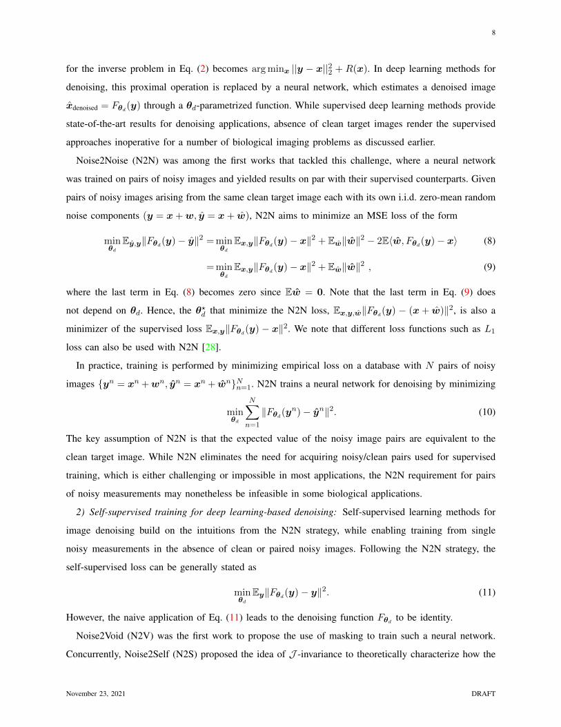
for the inverse problem in Eq. (2) becomes arg minx ||y − x||22 + R(x). In deep learning methods for

denoising, this proximal operation is replaced by a neural network, which estimates a denoised image

xdenoised = Fθd(y) through a θd-parametrized function. While supervised deep learning methods provide

state-of-the-art results for denoising applications, absence of clean target images render the supervised

approaches inoperative for a number of biological imaging problems as discussed earlier.

Noise2Noise (N2N) was among the first works that tackled this challenge, where a neural network

was trained on pairs of noisy images and yielded results on par with their supervised counterparts. Given

pairs of noisy images arising from the same clean target image each with its own i.i.d. zero-mean random

noise components (y = x+w, y = x+ w), N2N aims to minimize an MSE loss of the form

minθd

Ey,y‖Fθd(y)− y‖2 = minθd

Ex,y‖Fθd(y)− x‖2 + Ew‖w‖2 − 2E〈w, Fθd(y)− x〉 (8)

= minθd

Ex,y‖Fθd(y)− x‖2 + Ew‖w‖2 , (9)

where the last term in Eq. (8) becomes zero since Ew = 0. Note that the last term in Eq. (9) does

not depend on θd. Hence, the θ?d that minimize the N2N loss, Ex,y,w‖Fθd(y) − (x+ w)‖2, is also a

minimizer of the supervised loss Ex,y‖Fθd(y) − x‖2. We note that different loss functions such as L1

loss can also be used with N2N [28].

In practice, training is performed by minimizing empirical loss on a database with N pairs of noisy

images yn = xn +wn, yn = xn + wnNn=1. N2N trains a neural network for denoising by minimizing

minθd

N∑n=1

‖Fθd(yn)− yn‖2. (10)

The key assumption of N2N is that the expected value of the noisy image pairs are equivalent to the

clean target image. While N2N eliminates the need for acquiring noisy/clean pairs used for supervised

training, which is either challenging or impossible in most applications, the N2N requirement for pairs

of noisy measurements may nonetheless be infeasible in some biological applications.

2) Self-supervised training for deep learning-based denoising: Self-supervised learning methods for

image denoising build on the intuitions from the N2N strategy, while enabling training from single

noisy measurements in the absence of clean or paired noisy images. Following the N2N strategy, the

self-supervised loss can be generally stated as

minθd

Ey‖Fθd(y)− y‖2. (11)

However, the naive application of Eq. (11) leads to the denoising function Fθd to be identity.

Noise2Void (N2V) was the first work to propose the use of masking to train such a neural network.

Concurrently, Noise2Self (N2S) proposed the idea of J -invariance to theoretically characterize how the


9

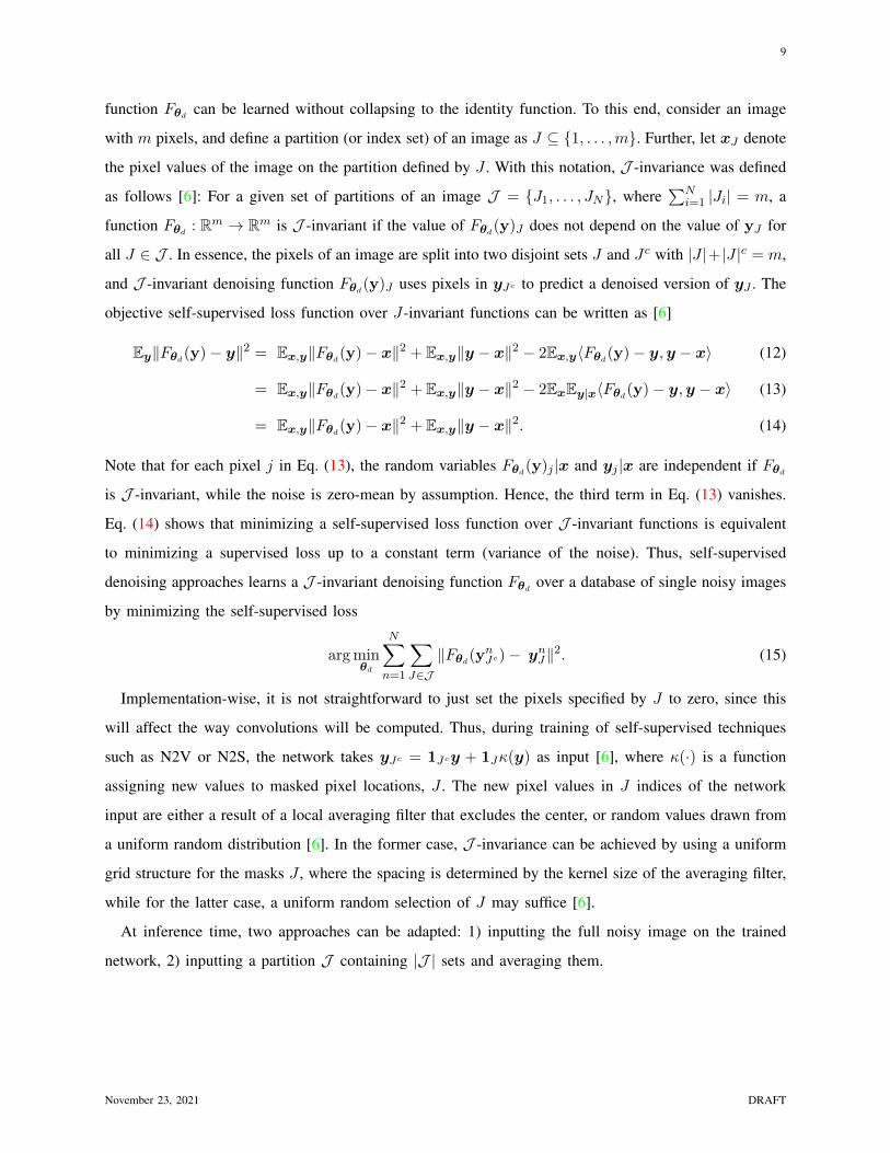
function Fθd can be learned without collapsing to the identity function. To this end, consider an image

with m pixels, and define a partition (or index set) of an image as J ⊆ 1, . . . ,m. Further, let xJ denote

the pixel values of the image on the partition defined by J . With this notation, J -invariance was defined

as follows [6]: For a given set of partitions of an image J = J1, . . . , JN, where∑N

i=1 |Ji| = m, a

function Fθd : Rm → Rm is J -invariant if the value of Fθd(y)J does not depend on the value of yJ for

all J ∈ J . In essence, the pixels of an image are split into two disjoint sets J and Jc with |J |+|J |c = m,

and J -invariant denoising function Fθd(y)J uses pixels in yJc to predict a denoised version of yJ . The

objective self-supervised loss function over J-invariant functions can be written as [6]

Ey‖Fθd(y)− y‖2 = Ex,y‖Fθd(y)− x‖2 + Ex,y‖y − x‖2 − 2Ex,y〈Fθd(y)− y,y − x〉 (12)

= Ex,y‖Fθd(y)− x‖2 + Ex,y‖y − x‖2 − 2ExEy|x〈Fθd(y)− y,y − x〉 (13)

= Ex,y‖Fθd(y)− x‖2 + Ex,y‖y − x‖2. (14)

Note that for each pixel j in Eq. (13), the random variables Fθd(y)j |x and yj |x are independent if Fθd

is J -invariant, while the noise is zero-mean by assumption. Hence, the third term in Eq. (13) vanishes.

Eq. (14) shows that minimizing a self-supervised loss function over J -invariant functions is equivalent

to minimizing a supervised loss up to a constant term (variance of the noise). Thus, self-supervised

denoising approaches learns a J -invariant denoising function Fθd over a database of single noisy images

by minimizing the self-supervised loss

arg minθd

N∑n=1

∑J∈J‖Fθd(ynJc)− ynJ‖2. (15)

Implementation-wise, it is not straightforward to just set the pixels specified by J to zero, since this

will affect the way convolutions will be computed. Thus, during training of self-supervised techniques

such as N2V or N2S, the network takes yJc = 1Jcy + 1Jκ(y) as input [6], where κ(·) is a function

assigning new values to masked pixel locations, J . The new pixel values in J indices of the network

input are either a result of a local averaging filter that excludes the center, or random values drawn from

a uniform random distribution [6]. In the former case, J -invariance can be achieved by using a uniform

grid structure for the masks J , where the spacing is determined by the kernel size of the averaging filter,

while for the latter case, a uniform random selection of J may suffice [6].

At inference time, two approaches can be adapted: 1) inputting the full noisy image on the trained

network, 2) inputting a partition J containing |J | sets and averaging them.


10

C. Self-supervised learning for image reconstruction

Self-supervised learning for image reconstruction neural networks provides a method for training

without paired measurement and reference data. One important line of work entails a method called

self-supervised learning via data undersampling (SSDU) [7], which generalizes the hold-out masking of

Section III-B2 for physics-guided image reconstruction.

For m-dimensional y, consider an index set Θ ⊆ 1, . . . ,m of all the available measurement coordi-

nates. In physics-guided DL reconstruction, the measurements interact with the neural network through

the data consistency operations. To this end, let HΘ(·) be the operator that outputs the measurement

coordinates corresponding to the index set Θ. In SSDU, hold-out masking is applied through these data

consistency operations. Thus, while the index set Θ is used in the data consistency units of the unrolled

network, the loss itself is calculated in the sensor domain on the indices specified by ΘC [7]. Hence,

SSDU minimizes the following self-supervised loss

minθr

1

N

N∑n=1

L(ynΘC , Hn

ΘC

(Fθr(ynΘ, H

nΘ))), (16)

where the output of the network is transformed back to the measurement domain by applying the forward

operator HnΘC at corresponding unseen locations in the training, ΘC . An overview of this strategy is given

in Fig. 2.

Fig. 2. Overview of the self-supervised learning methods for image reconstruction using hold-out masking. Black pixels denote

masked-out locations in the measurements and DC denotes the data consistency units of the unrolled network.

Note that unlike in the denoising scenario, the measurements for reconstruction can be in different

sensor domains, and thus the training algorithm does not have access to all the pixels of the image. Thus,


11

the concept of J -invariance is not applicable in this setting. Therefore, from a practical perspective, Θ

is chosen randomly. In [7], which focused on a Fourier-based sensor domain, a variable density masking

approach based on Gaussian probability densities was chosen. This inherently enabled a denser sampling

of the low-frequency content in Fourier space, which contain most of the energy for images, for use in the

data consistency units. However, a Gaussian density for masking requires a hyper-parameter controlling

its variance. Thus, in later works, SSDU was extended to a multi-mask setting [29], where multiple index

sets ΘlLl=1 were used to define the loss

minθr

1

N

N∑n=1

L∑l=1

L(ynΘC

l, Hn

ΘCl

(Fθr(ynΘl

;HnΘl

))). (17)

When utilizing multiple hold-out masks for the data consistency units, uniform random selection of the

masks becomes a natural choice, also eliminating the need for an additional hyper-parameter. Further-

more, the use of multiple ΘlLl=1 also leads to an improved performance, especially as H(·) becomes

increasingly ill-posed [29]. During inference time, SSDU-trained reconstruction uses all available m

measurements in y in the data consistency units for maximal performance [7].

Note that because the masking happens in the data consistency term, the implementation is simplified

to removing the relevant indices of the measurements for the data consistency components, and does not

require a modification of the regularization neural network component or its input, unlike in the denoising

scenario. This also enables a broader range of options for the loss L. While the negative log-likelihood,

c(x,y) of the RLS problem is an option, more advanced losses that better capture relevant features have

been used [7].

Apart from the hold-out masking strategy discussed here, there is a line of work that performs self-

supervision using a strategy akin to that described in Eq. (11), where all the measurements are used

in the network and for defining the loss [30]. More formally, such approaches aim to minimize a loss

function of the form

minθe

1

N

N∑n=1

L(yn, Hn

(Fθe(y

n;Hn))). (18)

We note that y denotes all the acquired measurements and H transforms the network output Fθe(·) to

sensor domain. However, the performance of such naive application of self-supervised learning approaches

suffers from noise amplification due to overfitting [7].

D. Biological Applications

1) Denoising: Even though N2N requires two independent noisy realizations of the target image for

unsupervised training, which may be hard to meet in general, it has been applied to light and electron


12

microscopy under Gaussian or Poisson noise scenarios. In cryo-TEM, the acquired datasets are inherently

noisy, since the electron dose is restricted to avoid sample destruction [26]. Cryo-CARE [26] was the

first work to show that the N2N can be applied to cryo-TEM data for denoising. Cryo-CARE was further

applied on 3D cryo-electron tomogram (cryo-ET) data showing its ability to denoise whole tomographic

volumes. Several other works have also extended N2N for denoising cryo-EM data [31], [32].

Fig. 3. Denoising results from fluorescence microscopy datasets Fluo-N2DH-GOWT1 and Fluo-C2DL-MSC using a traditional

denoising method BM3D and a self-supervised learning method Noise2Self (N2S). We note that supervised deep learning is not

applicable as these datasets contain only single noisy images.

N2V was the first work showing the denoising can be performed from single noisy measurements.

N2V has been extensively applied to EM datasets showing improved reconstruction quality compared to

conventional blind denoising methods such as BM3D [5]. In follow-up works, Bayesian post-processing

has been used to incorporate pixel-wise Gaussian [33] or histogram-based noise models [34] for further

improvements in the denoising performance. However, their application is limited as it requires the

knowledge of the noise model, which might be challenging to know as a prior in number of applications.

Moreover, the noise could be a mixture of noise type hence further hindering their applications. A follow-

up work on [34] show that the prior noise model knowledge requirement in probabilistic N2V models

can be tackled by learning the noise model directly from the noisy image itself via bootstrapping [35].

Another extension of this method, called structured N2V, was also proposed to mask a larger area rather


13

than a single pixel for removing structured noise in microscopy applications [8]. Similarly, Noise2Self

and its variants have also been applied to various microscopy datasets [6], [9].

Fig. 3 shows denoising results using a conventional denoising algorithm BM3D, and self-supervised

learning algorithm Noise2Self on two different microscopy datasets [36]. These datasets contain only

single noisy images, hence supervised deep learning and N2N can not be applied. Results show that self-

supervised learning approaches visually improve the denoising performance compared to conventional

denoising algorithms.

2) Reconstruction: DL-based ground-truth free reconstruction strategies has been applied in variety

of medical imaging applications. SSDU was one of the first self-supervised methods to be applied for

Fig. 4. Reconstruction results from an fMRI application [11] using conventional split-slice GRAPPA technique and self-

supervised multi-mask SSDU method [29]. (a) Split-slice GRAPPA exhibits residual artifacts in mid-brain (yellow arrows).

Multi-mask SSDU alleviates these, along with visible noise reduction. (b) Temporal SNR (tSNR) maps show substantial gain

with the self-supervised deep learning approach, particularly for subcortical areas and cortex further from the receiver coils.

(c) Phase maps for the two reconstructions show strong agreement, with multi-mask SSDU containing more voxels above the

coherence threshold.


14

physics-guided medical imaging reconstruction in MRI [7]. Concurrently, there were approaches inspired

by N2N that was used in non-Cartesian MRI [37], where pairs of undersampled measurements were used

for training. Similar to the denoising scenario, a main limitation of these methods is the requirement of

pairs of measurements, which may be challenging in some imaging applications. Furthermore, the naive

self-supervised learning strategy of Eq. (18) was also used for MRI reconstruction, by using all acquired

measurements for both input to the network and defining the loss [30]. However, this approach suffered

from noise amplification, as expected. Another line of work, called Noise2Inverse builds on N2S by

considering consistency with sensor domain measurements but focuses on a denoising-type application

in computed tomography [38].

While such self-supervised methods have found use in medical imaging, their utility in biological

imaging are just being explored. Recent work has started using such self-supervised deep learning methods

to functional MRI, which remains a critical biological imaging tool for neuroscientific discoveries that

expand our understanding of human perception and cognition. In a recent work [11], multi-mask SSDU

was applied to a Human Connectome Project style fMRI acquisition that was prospectively accelerated

by 5-fold simultaneous multi-slice imaging and 2-fold in-plane undersampling. Note that ground-truth

data for such high spatiotemporal resolution acquisitions cannot be acquired in practice, thus prohibiting

the use of supervised learning. The results shown in Fig. 4 indicate that the self-supervised deep learning

method based on multi-mask SSDU significantly outperforms the conventional reconstruction approaches,

both qualitatively in terms of visual quality, and quantitatively in terms of temporal signal-to-noise ratio.

IV. GENERATIVE MODEL-BASED METHODS

A. Overview

Generative models cover a large spectrum of research activities, which include variational autoencoder

(VAE) [39], generative adversarial network (GAN) [12], [13], [40], normalizing flow [41], optimal

transport (OT) [42], among others. Due to their popularity, there are so many variations, so one of

the main goals of this section is to provide a coherent geometric picture of generative models.

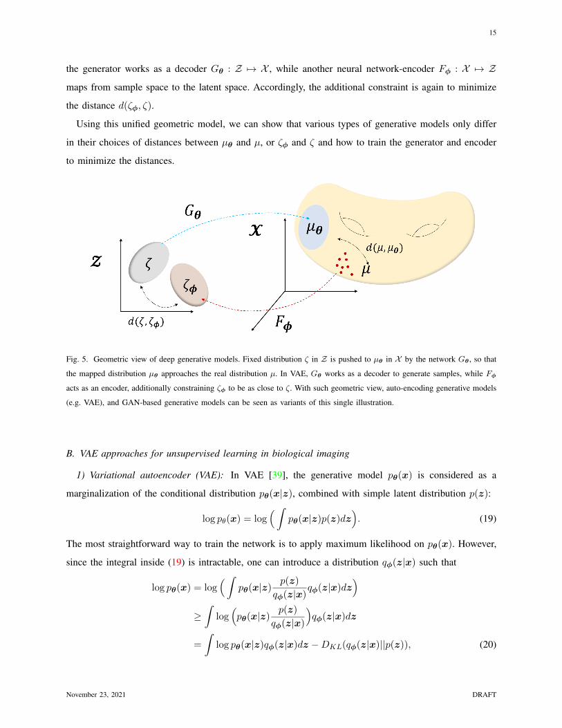
Specifically, our unified geometric view starts from Fig. 5. Here, the ambient image space is X , where

we can take samples with the real data distribution µ. If the latent space is Z , the generator G can be

treated as a mapping from the latent space to the ambient space, G : Z 7→ X , often realized by a deep

network with parameter θ, i.e. G , Gθ. Let ζ be a fixed distribution on the latent space, such as uniform

or Gaussian distribution. The generator Gθ pushes forward ζ to a distribution µθ = Gθ#ζ in the ambient

space X [42]. Then, the goal of the generative model training is to make µθ as close as possible to the

real data distribution µ. Additionally, for the case of auto-encoding type generative models (e.g. VAE),


15

the generator works as a decoder Gθ : Z 7→ X , while another neural network-encoder Fφ : X 7→ Z

maps from sample space to the latent space. Accordingly, the additional constraint is again to minimize

the distance d(ζφ, ζ).

Using this unified geometric model, we can show that various types of generative models only differ

in their choices of distances between µθ and µ, or ζφ and ζ and how to train the generator and encoder

to minimize the distances.

Fig. 5. Geometric view of deep generative models. Fixed distribution ζ in Z is pushed to µθ in X by the network Gθ , so that

the mapped distribution µθ approaches the real distribution µ. In VAE, Gθ works as a decoder to generate samples, while Fφ

acts as an encoder, additionally constraining ζφ to be as close to ζ. With such geometric view, auto-encoding generative models

(e.g. VAE), and GAN-based generative models can be seen as variants of this single illustration.

B. VAE approaches for unsupervised learning in biological imaging

1) Variational autoencoder (VAE): In VAE [39], the generative model pθ(x) is considered as a

marginalization of the conditional distribution pθ(x|z), combined with simple latent distribution p(z):

log pθ(x) = log(∫

pθ(x|z)p(z)dz). (19)

The most straightforward way to train the network is to apply maximum likelihood on pθ(x). However,

since the integral inside (19) is intractable, one can introduce a distribution qφ(z|x) such that

log pθ(x) = log(∫

pθ(x|z)p(z)

qφ(z|x)qφ(z|x)dz

)≥∫

log(pθ(x|z)

p(z)

qφ(z|x)

)qφ(z|x)dz

=

∫log pθ(x|z)qφ(z|x)dz −DKL(qφ(z|x)||p(z)), (20)


16

Fig. 6. VAE architecture. Fφ encodes x, and combined with random sample u to produce latent vector z. Gθ decodes the latent z

to acquire x. u is sampled from standard normal distribution for the reparameterization trick. (a) VAE [39]. (b) spatial-VAE [43],

disentangling translation/rotation features from different semantics. (c) DIVNOISING [44], enabling superviesd/unsupervised

training of denoising generative model by leveraging the noise model pNM (y|x).

where DKL is the Kullback–Leibler divergence (KL) divergence, and the first inequality comes from

Jensen’s inequality. The final term in (20) is called evidence lower bound (ELBO), or variational lower

bound in the context of variational inference. While infeasible to perform maximum likelihood on pθ(x)

directly, we can maximize the ELBO.

In the VAE, by using the reparametrization trick together with the Gaussian assumption [39], one has:

z = Fxφ (u) = µφ(x) + σφ(x) u, u ∼ N (0, I), (21)

where Fxφ (u) refers to the encoder function for a given image x which has another noisy input u, and

denotes the element-wise multiplication. Note that (21) enables back-propagation. Incorporating (21)


17

with (20) gives us the loss function to minimize for an end-to-end training of the VAE:

`V AE(θ, φ) (22)

=1

2

∫X

∫‖x−Gθ(µφ(x) + σφ(x) u)‖2r(u)dudµ(x)

+1

2

d∑i=1

∫X

(σ2i (x) + µ2

i (x)− log σ2i (x)− 1)dµ(x).

Here, the first term in (22) can be conceived as the reconstruction loss (d(µ, µθ) in Fig. 5), and the

second term is originated from KL divergence can be interpreted as penalty-imposing term (d(ζ, ζφ) in

Fig. 5).

Once the network is trained by minimizing (22), one notable advantage of VAE is that we can generate

samples from pθ(x|z) simply by sampling different noise vectors u. Specifically, the decoder has explicit

dependency on u, and the model output is expressed as

x(u) = Gθ(µφ(x) + σφ(x) u), u ∼ N (0, I). (23)

Notably, we can utilize (23) to sample multiple reconstructions by simply sampling different values of

u. Naturally, this method has been applied to many different fields, and in the following we review its

biological image applications.

2) Biological Applications: One notable application of VAE in the field of biological imaging is Bepler

et al. [43]. The work is motivated by the problem of modeling continuous 2D views of proteins from

single particle electron microscopy (EM). The goal of EM imaging is to estimate 3D electron density

of a given protein from multiple random noisy 2D projections. The first step in this process requires

estimation of the conformational states, often modeled with Gaussian mixture model, which is discrete.

Subsequently, modeling with Gaussian mixture models produces sub-optimal performance when aiming

to model protein conformations. Hence, to bridge this gap, Bepler et al. [43] propose spatial-VAE to

disentangle projection rotation and translation from the content of the projections.

Specifically, spatial-VAE [43] uses spatial generator network, first introduced in compositional pattern

producing networks (CPPNs), where the generator G takes in as input the spatial coordinates, and outputs

a pixel value. Moreover, as shown in Fig. 6(b), latent variable z is concatenated with additional parameters

ϕ,∆t, representing rotation, and translation, respectively. More precisely, the conditional distribution is

given as

log p(x|z) = log pθ(x|z, ϕ,∆t) (24)

=

n∑i=1

log pθ(xi|tiR(ϕ) + ∆t, z), (25)


18

where R(ϕ) = [cosϕ,− sinϕ; sinϕ, cosϕ] is the rotation matrix, and n is the dimensionality of the

image. It is straightforward to extend the encoder function to output disentangled representations, which

is given as

Fxφ (u) =

µz(x)

µϕ(x)

µ∆t(x)

+

σz(x)

sϕσϕ(x)

s∆tσ∆t(x)

u, (26)

where sϕ, s∆t are chosen differently for each problem set. (26) shows that Gaussian priors are used

for all the different parameters. Notably, by constructing spatial-VAE as given in (24), (26), translation

and rotation are successfully disentangled from other features. Consequently, continuous modeling of

parameter estimation in the particle projections of EM via spatial-VAE may substantially improve the

final reconstruction of 3D protein structure.

Another recent yet important work, dubbed DIVNOISING, utilizes a modified VAE for denoising

microscopy images [44]. As illustrated in Fig. 6(c), DIVNOISING tries to estimate the posterior p(x|y) ∝

pNM (y|x)p(x), where x is the true signal, y is the noise-corrupted version of x, p(x) is the prior, and

pNM (y|x) is the noise model, which is typically decomposed into a product of independent pixel-

wise noise models. Note that the input image y is not a clean image, as in the other works. Instead,

the encoder of DIVNOISING takes in a noisy image y to produce the latent vector z. In this VAE

setup, one can replace the conditional distribution pθ(x|z) with a known noise model in case we know

the corruption process, or learnable noise model in case we do not know the corruption process, and

unsupervised training is required. With this modification, one can perform semi-supervised training in

which the noise model is measured from paired calibration images, or bootstrapped from the noisy image.

More interestingly, it is also possible to perform unsupervised training with a modification to the decoder.

Once the VAE of DIVNOISING is trained, one can perform inference by varying the samples u, and

acquire multiple estimation of denoised images. When the user wants to acquire a point estimate of the

distribution, one can either choose the mean (i.e. MMSE) of the sampled images, or get maximum a

posteriori (MAP) estimate by iteratively applying mean shift clustering to the sampled images.

C. GAN approaches for unsupervised learning in biological imaging

1) Statistical Distance Minimization: In GAN, the generator G, and the discriminator D, play a

minimax game, complementing each other at every optimization step. Formally, the optimization process

is defined as [12]:

minG

maxDLGAN (D,G), (27)


19

where

LGAN (D,G) , Ex[logD(x)] + Ez[log(1−D(G(z)))]. (28)

Here, D(x) is called as the discriminator, which outputs a scalar in [0, 1] representing the probability

of the input x being a real sample. While the discriminator struggles to learn the classification task, the

generator tries to maximize the probability of D making a mistake. i.e. generating samples closer and

closer to the actual distribution of x.

To understand the geometric meaning of GAN, we first provide a brief review of f -GAN [13]. As the

name suggests, f -GAN starts with f -divergence as the statistical distance measure:

Df (µ||ν) =

∫Ωf

(dµ

dν

)dν (29)

where µ and ν are two statistical measures and µ is absolutely continuous with respect to ν. The key

observation is that instead of directly minimizing the f -divergence, a very interesting thing emerges if

we formulate its dual problem. In fact, the “dualization” trick is a common idea in generative models.

More specifically, if f is a convex function, the convex conjugate of its convex conjugate is the function

itself, i.e.

f(u) = f∗∗(u) = supτ∈I∗uτ − f∗(τ) (30)

if f∗ : I∗ 7→ R. Using this, for any class of functions τ mapping from X to R, we have the lower bound

Df (µ||ν) ≥ supτ∈I∗

∫Xτ(x)dµ(x)−

∫Xf∗(τ(x))dν(x) (31)

where f∗ : I∗ 7→ R is the convex conjugate of f . Using the following transform [13]

τ(x) = gf (V (x)) (32)

where V : X 7→ R without any constraint on the output range, and gf : R 7→ I∗ is an output activation

function that maps the output to the domain of f∗, f -GAN can be formulated as follows:

minG

maxgfLfGAN (G, gf ) (33)

where

LfGAN (G, gf ) , Ex∼µ [gf (V (x))]− Ez∼ζ [f∗(gf (V (G(z))))] . (34)

Here, different choices of the functions f, gf lead to distinct statistical measures and variations of f -

GANs, and for the case of Jensen-Shannon divergence, the original GAN as in (28) can be obtained.

Therefore, we can see that f -GANs are originated from statistical distance minimization.


20

Note that f -GAN interprets the GAN training as a statistical distance minimization after dualization.

Similar statistical distance minimization idea is employed for the Wasserstein GAN, but now with a real

metric in probability space rather than the divergence. More specifically, W-GAN minimizes the following

Wasserstein-1 norm:

d(µ, ν) ,W1(µ, ν) := minπ∈Π(µ,ν)

∫X×X

||x− x′||dπ(x,x′) (35)

where X is the ambient space, µ and ν are measures for the real data and generated data, respectively,

and π(x,x′) is the joint distribution with the marginals µ and ν, respectively.

Similar to f -GAN, rather than solving the complicated primal problem, a dual problem is solved.

The Kantorivich dual formulation from the optimal transport theory [42] leads to the following dual

formulation of the Wasserstein 1-norm:

d(µ, ν) = supD∈Lip1(X )

∫XD(x)dµ(x)−

∫XD(x′)dν(x′)

, (36)

where Lip1(X ) denotes the 1-Lipschitz function space with domain X , and D is the Kantorovich potential

that corresponds to the discriminator. Again, the measure ν is for the generated samples from latent

space Z with the measure ζ by generator G(z), z ∈ Z , so ν can be considered as pushforward measure

ν = G#µ. Therefore, Wasserstein 1-norm minimization problem can be equivalently represented by the

following minmax formulation:

LGAN (G,D) = minG

maxD∈Lip1(X )

∫XD(x)dµ(x)−

∫ZD(G(z))dζ(z)

.

This again confirms that W-GAN is originated from the statistical distance minimization problem.

2) Biological Applications: Since the birth of GAN, myriad of variants have been introduced in

literature and used for biological imaging applications. While the earlier works based on deep learning

focused on developing supervised methods for training (e.g. DeepSTORM [48]), the later works started

to employ conditional GAN (cGAN) into the reconstruction framework. More specifically, instead of

applying the original form of the GAN that generates images from random noise, these applications of

GAN are usually conditioned on specific input images.

For example, in the context of tomographic reconstruction, TomoGAN [49] aims at low dose tomo-

graphic reconstruction, where the generator takes in as input noisy images from low dose sinogram, and

maps it into the distribution of high dose images. Another model for 3-D tomographic reconstruction,

dubbed GANrec, was proposed in [50]. Different from TomoGAN, GANrec takes in as input the sinogram,

so that the generator needs also to learn the inverse mapping of the forward Radon transform. One

unique aspect is that the discriminator D learns the probability distribution of the clean sinogram. A

similar approach is used for super resolution [51], [52]. Specifically, in [52] a super-resolution (SR)


21

Fig. 7. Illustration of GAN-based methods for biological image reconstruction. (a) GAN [12], (b) pix2pix [45], (c)

AmbientGAN [46], (d) cryoGAN [47]. x,y denote data in the image domain, and the measurement domain, respectively. G,D

refers to generator, discriminator, respectively. H defines the function family of the forward measurement process, parameterized

with ϕ. Networks and variables that are marked in blue have learnable parameters optimized with gradient descent.

approach for Fourier ptychographic microscopy (FPM) is introduced, which proposes to reconstruct a

temporal sequence of cell images. Namely, only the first temporal sequence needs to be acquired in high

resolution to train the GAN network, after which the trained network is utilized for reconstruction at

the following temporal sequences. They also propose to use a Fourier domain loss, imposing additional

constraint on the content. For super-resolution microscopy, ANNA-PALM [51] was introduced to achieve

high-throughput in live-cell imaging, designed for accelerating PALM [53] by using much less number

of frames for restoring the true image.

These approaches that add condition to GANs in fact corresponds to pix2pix [45] or cGAN. Unlike

GANs illustrated in Fig. 7(a), which takes random noise vector z as input, pix2pix has additional loss

function Lcontent that measures the content distance (see Fig. 7(b)). Specifically, Lcontent measures the

content space distance between the generated image and the matched target image, which is used in

addition to the LGAN that measures the statistical distance. Therefore, pix2pix attempts to balance between

the paired data and unpaired target distributions. In fact, the addition of content loss is important to

regularize the inverse problems. Unfortunately, the methods cannot be regarded as unsupervised, since

the content loss Lcontent requires a matching label. Hence, to overcome this limitation, several works

that do not require any matched training data were proposed.

One interesting line of work stems from ambientGAN [46], where the forward measurement model


22

can be integrated into the framework. As in Fig. 7(c), the generator of ambientGAN generates a sample

from a random noise vector, and the discriminator takes in the measurement after the forward operator

Hϕ parameterized by ϕ, rather than the reconstructed image. Since only the function family of the

forward operator is known, the specific parameters are sampled from a feasible distribution, i.e. ϕ ∼ Pϕ.

Although the real and fake measurements do not match, ambientGAN enables training on the distribution,

rather than on realized samples. From a statistical distance minimization perspective, ambientGAN can

be interpreted as the dual problem for the statistical distance minimization in the measurement space. To

understand this claim, suppose that we use a W-GAN discriminator, and consider the following primal

form of the optimal transport problem that minimizes the 1-Wasserstein distance in the measurement

space:

minπ∈Π(µ,ν)

∫X×Y

‖Hϕ(x)− y‖dπ(x,y) . (37)

Then, the corresponding dual cost function becomes

LGAN (G,D) = maxD∈Lip1(X )

∫YD(y)dν(y)−

∫XD(Hϕ(x))dµ(x) (38)

= maxD∈Lip1(X )

∫YD(y)dν(y)−

∫XD(Hϕ(G(z)))dζ(z). (39)

where the last equation again comes from the change of variables formula. If we further assume that

ϕ ∈ Φ is random from the distribution Pϕ, (39) can be converted to

LGAN (G,D) = maxD∈Lip1(X )

∫YD(y)dν(y)−

∫Φ

∫XD(Hϕ(G(z)))dζ(z)dPϕ, (40)

which is equivalent to the ambientGAN loss function.

In the original work of ambientGAN, simple forward measurement models such as convolve+noise,

block+patch, 2D projection, etc. were used [46]. A variant of ambientGAN was introduced in the

context of cryo electron microscopy (cryo-EM) in [47], dubbed cryoGAN. Data acquisition in cryo-

EM is performed on multiple 3D copies of the same protein, called “particles”, which are assumed

to be structurally identical. To minimize the damage held on samples, multiple particles are frozen at

cryogenic temperatures, and all particles are simultaneously projected with parallel electron beam to

acquire projections. Here, unlike in the original ambientGAN, cryoGAN considers the latent particle

itself to be a learnable parameter. The overall flow of cryoGAN is as shown in Fig. 7(d). It is interesting

that there exists no generator in cryoGAN. Rather, x, the 3D particle to be reconstructed, is the starting

point of the overall flow. As in ambientGAN, x goes through a complex random forward measurement

process which involves 3D projection, convolution with the sampled kernel, and translation. Gradients

from the discriminator backpropagates to x, and x is updated directly at every optimization step. Unlike


23

conventional reconstruction methods for cryo-EM based on marginal maximum-likelihood which demands

estimation of the exact projection angles, cryoGAN does not require such expensive process. Note that the

loss function of cryoGAN is equivalent to (38). Therefore, by using the statistical distance minimization

approach, cryoGAN attempts to estimate the unknown 3D particular x directly without estimating the

projection angles for each particle.

Another, more recent work was proposed in [54], which is an upgraded version of cryoGAN, called

multi-cryoGAN. While cryoGAN is able to reconstruct a single particle that explains the measured

projections, it does not take into account that the measured particle is not rigid, and hence can have

multiple conformations. To sidestep this issue, multi-cryoGAN takes an approach more similar to the

original ambientGAN, where a random noise vector is sampled from a distribution, and the generator G

is responsible for mapping the noise vector into the 3D particle. The rest of the steps follow the same

procedure in ambientGAN, although the complicated forward measurement for cryo-EM is utilized. One

advantage of multi-cryoGAN is that once the networks are trained, multiple conformations of the particle

can be sampled by varying the noise vector z. Subsequently, this introduces flexibility in the networks.

A related work was also proposed in the context of unsupervised MRI reconstruction in [55]. More

specifically, this work follows the overall flow depicted in Fig. 7(c). However, the input is not a random

noise vector, but an aliased image, inverse Fourier-transformed from the under-sampled k-space mea-

surement. The generator is responsible for conditional reconstruction, making the input image free of

aliasing artifacts. The reconstruction goes through the random measurement process in the context of MR

imaging, which corresponds to Fourier transform, and random masking. Then, the discriminator matches

the distribution of the aliased image, inverse Fourier transformed from the measurement. The authors

showed that even with the unsupervised learning process without any ground-truth data, reconstruction

of fair quality could be performed.

D. Optimal transport driven CycleGAN approaches for unsupervised learning for biological imaging

Another important line of work for unsupervised biological reconstruction comes from optimal transport

driven cycleGAN (OT-cycleGAN) [16], which is a generalization of the original cycleGAN [15]. Unlike

pix2pix, cycleGAN does not utilize Lcontent from paired label, so it is fully unsupervised. In contrast to

the ambientGAN or cryoGAN, which is based on the statistical distance minimization in the measurement

space, cycleGAN attempts to minimizes the statistical distance in both measurement and the image domain

simultaneously, which makes the algorithm more stable.

OT-cycleGAN can be understood from the geometric description illustrated in Fig. 8. Specifically, let

us consider the target image probability space X equipped with the measure µ, and the measurement


24

probability space Y equipped with the measure ν as in Fig. 8. In order to achieve a mapping from Y

to X and vice versa, we can try to find the transportation mapping from the measure space (Y, ν) to

(X , µ) with the generator Gθ : Y 7→ X , a neural network parameterized with θ, and the mapping from

the measure space (X , µ) to (Y, ν) with the forward mapping generator Hϕ : X 7→ Y , parametrized with

v. In other words, the generator Gθ pushes forward the measure ν in X to µθ in Y , and Hϕ pushes

forward the measure µ in Y to the measure νϕ in X . Then, our goal is to minimize the statistical distance

d(µ, µθ) between µ and µθ, and the distance d(ν, νϕ) between ν and νϕ simultaneously.

Fig. 8. Geometric view of cycleGAN. (Y, ν) is mapped to (X , µ) with Gθ , while Hϕ does the opposite. The two mappers,

i.e. generators are optimized by simultaneously minimizing d(µ, µθ), d(ν, νϕ).

Specifically, if we use the Wasserstein-1 metric, the statistical distance in each space can be computed

as:

W1(µ, µθ) = infπ∈Π(µ,ν)

∫X×Y

‖x−Gθ(y)‖dπ(x,y) (41)

W1(ν, νϕ) = infπ∈Π(µ,ν)

∫X×Y

‖y −Hϕ(x)‖dπ(x,y). (42)

If we minimize them separately, the optimal joint distribution π∗ for each problem may be different.

Accordingly, we attempt to find the unique joint distribution which minimizes the two distances simul-

taneously using the following primal formulation:

minπ∈Π(µ,ν)

∫X×Y

‖x−Gθ(y)‖+ ‖Hϕ(x)− y‖dπ(x,y). (43)

One interesting finding made in [16] is that the primal cost in (43) can be represented in a dual formulation

minθ,ϕ

maxDX ,DY

LcycleGAN (θ,ϕ;DX , DY ), (44)


25

where

LcycleGAN (θ,ϕ;DX , DY ) , λLcycle(θ,ϕ) + LGAN (θ,ϕ;DX , DY ), (45)

where Lcycle,LGAN refers to cycle-consistency loss and discriminator GAN loss, respectively. DX and

DY are discriminators in X and Y . The corresponding OT-cycleGAN network architecture can be

represented as in Fig. 9.

In fact, one of the most important reasons OT-cycleGAN is suitable for biological reconstruction

problems, is that the prior knowledge about the imaging physics can be flexibly incorporated into the

design of OT-cycleGAN to simplify the network. Specifically, in many biological imaging problems, the

forward mapping Hϕ is known or partially known. In this case, we do not need to use complex deep

neural networks for forward measurement operator. Instead, we use a deterministic or parametric form

of the forward measurement operation, which makes the training much simpler.

In addition, in comparison with ambientGAN in (37), OT-cycleGAN primal formulation in (43) has

an additional term ‖x − Gθ(y)‖ that enforces the reconstruction images to match the target image

distributions, which further regularizes the reconstruction process. In fact, the resulting OT-cycleGAN

formulation is closely related to the classical RLS formulation in (2). Specifically, the transportation

cost in (43) resembles closely to the cost function in (2), except that regularization term R(x) in (2) is

replaced by the deep learning-based inverse path penalty term ‖x−Gθ(y)‖.

However, instead of solving x directly as in (2), OT-cycleGAN tries to find the joint distribution π∗ that

minimizes the average cost for all combination of x ∈ X and y ∈ Y . This suggests that OT-cycleGAN

is a stochastic generalization of the RLS, revealing an important link to the classical RLS approaches.

Fig. 9. Network architecture of cycleGAN. Gθ : Y 7→ X , Hϕ : X 7→ Y are the generators responsible for inter-domain

mapping. DX , DY are discriminators, constructing LGAN . GAN loss is simultaneously optimized together with Lcycle

1) Applications: Thanks to the versatility of cycleGAN, which learns the distributions in both mea-

surement and image spaces, OT-cycleGAN has been adopted to numerous tasks in biological imaging.


26

For example, cycleGAN was used with linear blur kernel for blind and non-blind deconvolution in

[17]. More specifically, [17] focused on the fact that the forward operator of deconvolution microscopy

is usually represented as a convolution with a point spread function (PSF). Hence, even for the non-blind

case, the forward mapping Hϕ : X 7→ Y is partially known as a linear convolution. Leveraging this

property, one of the generators in cycleGAN, F in Fig. 9 is replaced with a linear convolutional layer,

taking into the account the physics of deconvolution microscopy. By exploiting the physical property,

the reconstruction quality of deconvolution microscopy is further enhanced. Even more, in the case of

non-blind microscopy, it was shown that the forward mapping is deterministic so that optimization with

respect to the discriminator DY is no longer necessary, which simplifies the network architecture, and

makes the training more robust. A similar simplification of cycleGAN leveraging the imaging physics

of microscopy was also proposed in super-resolution microscopy [16]. Interestingly, the simplified form

of cycleGAN could generate reconstructions of higher resolution, quantified in Fourier ring correlation

(FRC). Other than simplifying the mapping Hϕ : X 7→ Y with a linear blind kernel, a deterministic

k-space sub-sampling operator for MR imaging was extensively studied [56]–[58].

When such simplification is not possible, the most general form of cycleGAN, where two sets of

generator/discriminator pair are used, can be utilized, but still the key concept of statistical distance

minimization can be utilized in the design. One work, which utilizes cycleGAN for deconvolution

microscopy is [61], where the authors propose to use spatial constraint loss on top of cyclic loss to

further impose emphasis on the alignment of the reconstruction. The cycleGAN method adopted in [61]

is a 2D cycleGAN, so the authors propose a 3-way volume averaging of the reconstructed results in the

x − y, y − z, and x − z plane. However, in contrast to [17], two neural network based generators are

used for both forward and inverse paths. In another work, an unsupervised reconstruction method called

projectionGAN for optical diffraction tomography (ODT) was proposed [59]. Missing cone problem in

ODT arises because the measurement angles of the imaging device does not cover the whole solid angle,

hence leaving a cone-shaped wedge in the k-space empty. The authors focus on the fact that when parallel

beam projection is performed to the 3D distribution of refractive-index (RI), the acquired projections are

sharp with high quality when the projection angle is aligned with the measurement angle (YΩ), and

are blurry and with artifacts when the projection angle is not aligned (YΩc). Hence, the resolution of

the blurry projections are enhanced via distribution matching between YΩ and YΩc with cycleGAN,

after which follows filtered back projection (FBP) to acquire the final reconstruction from the enhanced

projections. By the projectionGAN enhancement step, the missing cone artifacts are greatly resolved,

achieving accurate reconstruction, as illustrated in Fig. 10. As shown in the figure, with other methods

we see elongation along optical axes which makes the structure of the cell vague and noisy (x − z,


27

Fig. 10. ProjectionGAN for the reconstruction of ODT [59]. (a) Conventional Rytov reconstruction via Fourier binning, (b)

Gerchberg-Papoulis (GP) algorithm [60], (c) model-based iterative method using the total variation (TV), and (b) reconstruction

via projectionGAN. Artifacts including elongation along the optical axes can be seen in the x − z, y − z cutview of (a),(c).

The result shown in (b) is contaminated with resdual noise in the x− z, y − z planes. Result shown in (d) has high-resolution

reconstruction without such artifacts, along with boosted RI values.

y − z plane). This problem is much resolved with ProjectionGAN, where we observe clear boundaries

and micro-cellular structures. Underestimated RI values are also corrected.

For optical microscopy, content-preserving cycleGAN (c2GAN) was proposed [62], showing applica-


28

bility of cycleGAN to various imagnig modalities and data configurations. c2GAN introduces saliency

constraint to cycleGAN framework, where the saliency constraint imposes an additional cycle-consistency

after thresholding the images at certain values. This simple fix is derived from the fact that many biological

images contain salient regions of higher intensity, while the rest is covered with low-intensity background.

Thus, by adding the saliency constraint, cycleGAN can concentrate more on the salient features. The

authors applied c2GAN to biological image denoising, restoration, super-resolution, histological coloriza-

tion, and image translation such as phase contrast images to flourescence-labeled images, showing how

cycleGAN can be easily adopted to many different tasks of biological imaging.

V. DISCUSSION

A. Open problems

The performance improvement from DL-based techniques has been one of the main drivers of their

mainstream adaptation in a large number of imaging applications. This is largely driven by the application-

specific tailoring of the regularization strategies during the training phase of DL reconstruction algorithms.

Thus, the use of unsupervised training strategies in the absence of matched reference data is critical for

the continued utility of DL reconstruction in a number of biological imaging scenarios.

This overview article focused on two unsupervised learning strategies that tackle seemingly different

aspects of the training process. Self-supervised learning uses parts of the available data to predict the

remaining parts, in effect repurposing some of the available data as supervisory labels. Generative models

aim to minimize a statistical distance measure between an underlying target distribution and the generated

data distribution. While these goals do not necessarily appear complementary, there are self-supervisory

methods, such as content generation, which utilize properties of generative models. Similarly, there are

generative models that utilize concepts of prediction of data from self-supervision [63]. Thus, a synergistic

viewpoint that tie these two different lines of work for unsupervised learning of image reconstruction

approaches may further improve the performance of DL-based methods in the absence of reference

training data.

Self-supervised learning techniques have enabled the training on large datasets containing only noisy

or incomplete measurements. However, in some biological applications, it may not always be feasible

to obtain large training datasets. Hence, it is desirable to perform training from a single measurement.

However, training on a single noisy measurement often leads to overfitting, requiring early stopping

[64]. Recently, self-supervised learning methods have been proposed to perform reconstruction and

enhancement for a single measurement without overfitting [65], [66]. Particularly, for image denoising, a

dropout regularization technique has been incorporated with a hold-out self-supervised learning framework


29

for avoiding overfitting [65]. For image reconstruction, a zero-shot self-supervised learning approach has

been proposed to split available measurements: two of which are used in the data consistency and the loss

as in SSDU, while the third is used as a validation set to determine the early stopping criteria [66]. These

works may be essential for developing new frameworks for training biological imaging applications with

sparse datasets.

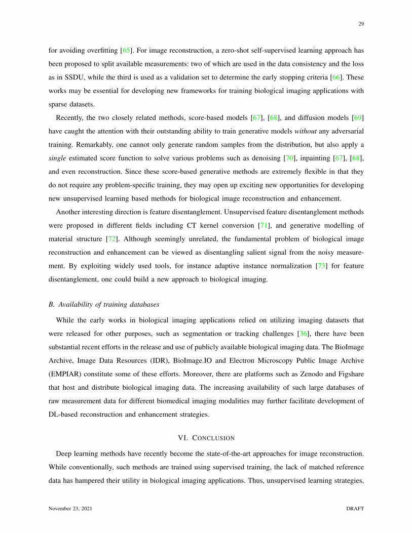
Recently, the two closely related methods, score-based models [67], [68], and diffusion models [69]

have caught the attention with their outstanding ability to train generative models without any adversarial

training. Remarkably, one cannot only generate random samples from the distribution, but also apply a

single estimated score function to solve various problems such as denoising [70], inpainting [67], [68],

and even reconstruction. Since these score-based generative methods are extremely flexible in that they

do not require any problem-specific training, they may open up exciting new opportunities for developing

new unsupervised learning based methods for biological image reconstruction and enhancement.

Another interesting direction is feature disentanglement. Unsupervised feature disentanglement methods

were proposed in different fields including CT kernel conversion [71], and generative modelling of

material structure [72]. Although seemingly unrelated, the fundamental problem of biological image

reconstruction and enhancement can be viewed as disentangling salient signal from the noisy measure-

ment. By exploiting widely used tools, for instance adaptive instance normalization [73] for feature

disentanglement, one could build a new approach to biological imaging.

B. Availability of training databases

While the early works in biological imaging applications relied on utilizing imaging datasets that

were released for other purposes, such as segmentation or tracking challenges [36], there have been

substantial recent efforts in the release and use of publicly available biological imaging data. The BioImage

Archive, Image Data Resources (IDR), BioImage.IO and Electron Microscopy Public Image Archive

(EMPIAR) constitute some of these efforts. Moreover, there are platforms such as Zenodo and Figshare

that host and distribute biological imaging data. The increasing availability of such large databases of

raw measurement data for different biomedical imaging modalities may further facilitate development of

DL-based reconstruction and enhancement strategies.

VI. CONCLUSION

Deep learning methods have recently become the state-of-the-art approaches for image reconstruction.

While conventionally, such methods are trained using supervised training, the lack of matched reference

data has hampered their utility in biological imaging applications. Thus, unsupervised learning strategies,


30

encompassing both self-supervised methods and generative models, have been proposed, showing great

promise. Self-supervised methods devise a way to create supervisory labels from the incomplete mea-

surement data itself to train the model. Hold-out masking strategy is especially useful for both image

denoising and reconstruction. With recent advances, one can perform training with as little as a single

noisy measurement. Generative model based methods encompass diverse methods for image denoising

and reconstruction, with VAE and GAN being the two most prominent strategies. Both methods can be

seen as the optimization problem of statistical minimization, with different choices for statistical distance

measure leading to seemingly unrelated methods for training the generative model.

These strategies are still being developed and applied to biological imaging scenarios, creating op-

portunities for the broader signal processing community in terms of new technical developments and

applications.

REFERENCES

[1] D. L. Donoho, “Compressed sensing,” IEEE Transactions on Information Theory, vol. 52, no. 4, pp. 1289–1306, 2006. 2

[2] A. Chambolle, “An algorithm for total variation minimization and applications,” Journal of Mathematical Imaging and

Vision, vol. 20, no. 1-2, pp. 89–97, 2004. 2

[3] E. T. Jaynes, “On the rationale of maximum-entropy methods,” Proceedings of the IEEE, vol. 70, no. 9, pp. 939–952,

1982. 2

[4] L. Jing and Y. Tian, “Self-supervised visual feature learning with deep neural networks: A survey,” IEEE Transactions on

Pattern Analysis and Machine Intelligence, 2020. 2, 7

[5] A. Krull, T.-O. Buchholz, and F. Jug, “Noise2Void-learning denoising from single noisy images,” in Proceedings of the

IEEE Conference on Computer Vision and Pattern Recognition, 2019, pp. 2129–2137. 2, 12

[6] J. Batson and L. Royer, “Noise2Self: blind denoising by self-supervision,” in Proceedings of the International Conference

on Machine Learning, 2019, pp. 524–533. 2, 9, 13

[7] B. Yaman, S. A. H. Hosseini, S. Moeller, J. Ellermann, K. Ugurbil, and M. Akcakaya, “Self-supervised learning of

physics-guided reconstruction neural networks without fully-sampled reference data,” Magnetic Resonance in Medicine,

vol. 84, no. 6, pp. 3172–3191, Dec 2020. 2, 10, 11, 14

[8] C. Broaddus, A. Krull, M. Weigert, U. Schmidt, and G. Myers, “Removing structured noise with self-supervised blind-spot

networks,” in 2020 IEEE 17th International Symposium on Biomedical Imaging (ISBI), 2020, pp. 159–163. 2, 13

[9] Y. Xie, Z. Wang, and S. Ji, “Noise2Same: optimizing a self-supervised bound for image denoising,” in Advances in Neural

Information Processing Systems, 2020, vol. 33, pp. 20320–20330. 2, 13

[10] T.-O. Buchholz, A. Krull, R. Shahidi, G. Pigino, G. Jekely, and F. Jug, “Content-aware image restoration for electron

microscopy,” Methods in Cell Biology, vol. 152, pp. 277–289, 2019. 2, 6

[11] O. B. Demirel, B. Yaman, L. Dowdle, S. Moeller, L. Vizioli, E. Yacoub, J. Strupp, C. A. Olman, K. Ugurbil, and

M. Akcakaya, “Improved simultaneous multi-slice functional MRI using self-supervised deep learning,” arXiv: 2105.04532,

2021. 2, 13, 14

[12] I. Goodfellow, J. Pouget-Abadie, M. Mirza, B. Xu, D. Warde-Farley, S. Ozair, A. Courville, and Y. Bengio, “Generative

adversarial nets,” in Advances in Neural Information Processing Systems, 2014, pp. 2672–2680. 3, 14, 18, 21


31

[13] S. Nowozin, B. Cseke, and R. Tomioka, “f-GAN: training generative neural samplers using variational divergence

minimization,” in Advances in Neural Information Processing Systems, 2016, vol. 29. 3, 14, 19

[14] L. Ruthotto and E. Haber, “An introduction to deep generative modeling,” arXiv preprint arXiv:2103.05180, 2021. 3

[15] J.-Y. Zhu, T. Park, P. Isola, and A. A. Efros, “Unpaired image-to-image translation using cycle-consistent adversarial

networks,” in Proceedings of the IEEE International Conference on Computer Vision, 2017, pp. 2223–2232. 3, 23

[16] B. Sim, G. Oh, J. Kim, C. Jung, and J. C. Ye, “Optimal transport driven CycleGAN for unsupervised learning in inverse

problems,” SIAM Journal on Imaging Sciences, vol. 13, no. 4, pp. 2281–2306, 2020. 3, 23, 24, 26

[17] S. Lim, H. Park, S.-E. Lee, S. Chang, B. Sim, and J. C. Ye, “CycleGAN with a blur kernel for deconvolution microscopy:

Optimal transport geometry,” IEEE Transactions on Computational Imaging, vol. 6, pp. 1127–1138, 2020. 3, 26

[18] A. Beck, First-order methods in optimization, SIAM, 2017. 3

[19] E. Bostan, U. S. Kamilov, and L. Waller, “Learning-based image reconstruction via parallel proximal algorithm,” IEEE

Signal Processing Letters, vol. 25, no. 7, pp. 989–993, 2018. 3

[20] S. H. Chan, X. Wang, and O. A. Elgendy, “Plug-and-play admm for image restoration: Fixed-point convergence and

applications,” IEEE Transactions on Computational Imaging, vol. 3, no. 1, pp. 84–98, 2016. 4

[21] Y. Romano, M. Elad, and P. Milanfar, “The little engine that could: Regularization by denoising (red),” SIAM Journal on

Imaging Sciences, vol. 10, no. 4, pp. 1804–1844, 2017. 4

[22] S. Wang, Z. Su, L. Ying, X. Peng, S. Zhu, F. Liang, D. Feng, and D. Liang, “Accelerating magnetic resonance imaging

via deep learning,” in 2016 IEEE 13th International Symposium on Biomedical Imaging (ISBI). IEEE, 2016, pp. 514–517.

5

[23] V. Monga, Y. Li, and Y. C. Eldar, “Algorithm unrolling: Interpretable, efficient deep learning for signal and image

processing,” IEEE Signal Processing Magazine, vol. 38, no. 2, pp. 18–44, 2021. 5

[24] F. Knoll, K. Hammernik, C. Zhang, S. Moeller, T. Pock, D. K. Sodickson, and M. Akcakaya, “Deep-learning methods

for parallel magnetic resonance imaging reconstruction,” IEEE Signal Processing Magazine, vol. 37, no. 1, pp. 128–140,

2020. 5

[25] M. J. Muckley, B. Riemenschneider, A. Radmanesh, S. Kim, G. Jeong, J. Ko, Y. Jun, H. Shin, D. Hwang, M. Mostapha,

et al., “Results of the 2020 fastmri challenge for machine learning mr image reconstruction,” IEEE Transactions on

Medical Imaging, 2021. 5

[26] T.-O. Buchholz, M. Jordan, G. Pigino, and F. Jug, “Cryo-care: content-aware image restoration for cryo-transmission

electron microscopy data,” in 2019 IEEE 16th International Symposium on Biomedical Imaging (ISBI 2019). IEEE, 2019,

pp. 502–506. 6, 12

[27] J. Icha, M. Weber, J. C. Waters, and C. Norden, “Phototoxicity in live fluorescence microscopy, and how to avoid it,”

BioEssays, vol. 39, no. 8, pp. 1700003, 2017. 6

[28] J. Lehtinen, J. Munkberg, J. Hasselgren, S. Laine, T. Karras, M. Aittala, and T. Aila, “Noise2Noise: Learning image

restoration without clean data,” in Proceedings of the 35th International Conference on Machine Learning. 2018, vol. 80,

pp. 2965–2974, PMLR. 8

[29] B. Yaman, S. A. H. Hosseini, S. Moeller, J. Ellermann, K. Ugurbil, and M. Akcakaya, “Ground-truth free multi-mask

self-supervised physics-guided deep learning in highly accelerated mri,” in 2021 IEEE 18th International Symposium on

Biomedical Imaging (ISBI). IEEE, 2021, pp. 1850–1854. 11, 13

[30] O. Senouf, S. Vedula, T. Weiss, A. Bronstein, O. Michailovich, and M. Zibulevsky, “Self-supervised learning of inverse

problem solvers in medical imaging,” in Domain Adaptation and Representation Transfer and Medical Image Learning

with Less Labels and Imperfect Data, pp. 111–119. Springer, 2019. 11, 14


32

[31] D. Tegunov and P. Cramer, “Real-time cryo-electron microscopy data preprocessing with warp,” Nature methods, vol. 16,

no. 11, pp. 1146–1152, 2019. 12

[32] T. Bepler, K. Kelley, A. J. Noble, and B. Berger, “Topaz-denoise: general deep denoising models for cryoem and cryoet,”

Nature communications, vol. 11, no. 1, pp. 1–12, 2020. 12

[33] S. Laine, T. Karras, J. Lehtinen, and T. Aila, “High-quality self-supervised deep image denoising,” Advances in Neural

Information Processing Systems, vol. 32, pp. 6970–6980, 2019. 12

[34] A. Krull, T. Vicar, M. Prakash, M. Lalit, and F. Jug, “Probabilistic noise2void: Unsupervised content-aware denoising,”

Frontiers in Computer Science, vol. 2, pp. 5, 2020. 12

[35] M. Prakash, M. Lalit, P. Tomancak, A. Krul, and F. Jug, “Fully unsupervised probabilistic noise2void,” in 2020 IEEE

17th International Symposium on Biomedical Imaging (ISBI). IEEE, 2020, pp. 154–158. 12

[36] V. Ulman, M. Maska, K. E. Magnusson, O. Ronneberger, C. Haubold, N. Harder, P. Matula, P. Matula, D. Svoboda,

M. Radojevic, et al., “An objective comparison of cell-tracking algorithms,” Nature methods, vol. 14, no. 12, pp. 1141,

2017. 13, 29

[37] J. Liu, Y. Sun, C. Eldeniz, W. Gan, H. An, and U. S. Kamilov, “Rare: Image reconstruction using deep priors learned

without groundtruth,” IEEE Journal of Selected Topics in Signal Processing, vol. 14, no. 6, pp. 1088–1099, 2020. 14

[38] A. A. Hendriksen, D. M. Pelt, and K. J. Batenburg, “Noise2inverse: Self-supervised deep convolutional denoising for

tomography,” IEEE Transactions on Computational Imaging, vol. 6, pp. 1320–1335, 2020. 14

[39] D. P. Kingma and M. Welling, “Auto-Encoding Variational Bayes,” in 2nd International Conference on Learning

Representations, ICLR, 2014. 14, 15, 16

[40] M. Arjovsky, S. Chintala, and L. Bottou, “Wasserstein generative adversarial networks,” in Proceedings of the 34th

International Conference on Machine Learning. 06–11 Aug 2017, vol. 70 of Proceedings of Machine Learning Research,

pp. 214–223, PMLR. 14

[41] L. Dinh, D. Krueger, and Y. Bengio, “NICE: non-linear independent components estimation,” in 3rd International

Conference on Learning Representations, ICLR, 2015. 14

[42] C. Villani, Optimal transport: Old and new, vol. 338, Springer Science & Business Media, 2008. 14, 20

[43] T. Bepler, E. D. Zhong, K. Kelley, E. Brignole, and B. Berger, “Explicitly disentangling image content from translation

and rotation with spatial-vae,” arXiv preprint arXiv:1909.11663, 2019. 16, 17

[44] M. Prakash, A. Krull, and F. Jug, “Fully unsupervised diversity denoising with convolutional variational autoencoders,”

arXiv preprint arXiv:2006.06072, 2020. 16, 18

[45] P. Isola, J.-Y. Zhu, T. Zhou, and A. A. Efros, “Image-to-image translation with conditional adversarial networks,” in

Proceedings of the IEEE conference on computer vision and pattern recognition, 2017, pp. 1125–1134. 21

[46] A. Bora, E. Price, and A. G. Dimakis, “AmbientGAN: generative models from lossy measurements,” in 6th International

Conference on Learning Representations, ICLR, 2018. 21, 22

[47] H. Gupta, M. T. McCann, L. Donati, and M. Unser, “CryoGAN: a new reconstruction paradigm for single-particle Cryo-EM

via deep adversarial learning,” BioRxiv, 2020. 21, 22

[48] E. Nehme, L. E. Weiss, T. Michaeli, and Y. Shechtman, “Deep-STORM: super-resolution single-molecule microscopy by

deep learning,” Optica, vol. 5, no. 4, pp. 458–464, 2018. 20

[49] Z. Liu, T. Bicer, R. Kettimuthu, D. Gursoy, F. De Carlo, and I. Foster, “TomoGAN: low-dose synchrotron x-ray tomography

with generative adversarial networks: discussion,” JOSA A, vol. 37, no. 3, pp. 422–434, 2020. 20

[50] X. Yang, M. Kahnt, D. Bruckner, A. Schropp, Y. Fam, J. Becher, J.-D. Grunwaldt, T. L. Sheppard, and C. G. Schroer,


33

“Tomographic reconstruction with a generative adversarial network,” Journal of synchrotron radiation, vol. 27, no. 2, 2020.

20

[51] W. Ouyang, A. Aristov, M. Lelek, X. Hao, and C. Zimmer, “Deep learning massively accelerates super-resolution

localization microscopy,” Nature biotechnology, vol. 36, no. 5, pp. 460–468, 2018. 20, 21

[52] T. Nguyen, Y. Xue, Y. Li, L. Tian, and G. Nehmetallah, “Deep learning approach for Fourier ptychography microscopy,”

Optics express, vol. 26, no. 20, pp. 26470–26484, 2018. 20

[53] E. Betzig, G. H. Patterson, R. Sougrat, O. W. Lindwasser, S. Olenych, J. S. Bonifacino, M. W. Davidson, J. Lippincott-

Schwartz, and H. F. Hess, “Imaging intracellular fluorescent proteins at nanometer resolution,” Science, vol. 313, no. 5793,

pp. 1642–1645, 2006. 21

[54] H. Gupta, T. H. Phan, J. Yoo, and M. Unser, “Multi-CryoGAN: Reconstruction of continuous conformations in Cryo-EM

using generative adversarial networks,” in European Conference on Computer Vision. Springer, 2020, pp. 429–444. 23

[55] E. K. Cole, J. M. Pauly, S. S. Vasanawala, and F. Ong, “Unsupervised MRI reconstruction with generative adversarial

networks,” arXiv preprint arXiv:2008.13065, 2020. 23

[56] G. Oh, B. Sim, H. Chung, L. Sunwoo, and J. C. Ye, “Unpaired deep learning for accelerated MRI using optimal transport

driven cycleGAN,” IEEE Transactions on Computational Imaging, vol. 6, pp. 1285–1296, 2020. 26

[57] H. Chung, E. Cha, L. Sunwoo, and J. C. Ye, “Two-stage deep learning for accelerated 3D time-of-flight MRA without

matched training data,” Medical Image Analysis, p. 102047, 2021. 26

[58] E. Cha, H. Chung, E. Y. Kim, and J. C. Ye, “Unpaired training of deep learning tMRA for flexible spatio-temporal

resolution,” IEEE Transactions on Medical Imaging, 2020. 26

[59] H. Chung, J. Huh, G. Kim, Y. K. Park, and J. C. Ye, “Unsupervised missing cone deep learning in optical diffraction

tomography,” arXiv preprint arXiv:2103.09022, 2021. 26, 27

[60] R. Gerchberg, “Super-resolution through error energy reduction,” Optica Acta: International Journal of Optics, vol. 21,

no. 9, pp. 709–720, 1974. 27

[61] S. Lee, S. Han, P. Salama, K. W. Dunn, and E. J. Delp, “Three dimensional blind image deconvolution for fluorescence

microscopy using generative adversarial networks,” in 2019 IEEE 16th International Symposium on Biomedical Imaging

(ISBI 2019). IEEE, 2019, pp. 538–542. 26

[62] X. Li, G. Zhang, H. Qiao, F. Bao, Y. Deng, J. Wu, Y. He, J. Yun, X. Lin, H. Xie, et al., “Unsupervised content-preserving

transformation for optical microscopy,” Light: Science & Applications, vol. 10, no. 1, pp. 1–11, 2021. 27

[63] E. Bostan, R. Heckel, M. Chen, M. Kellman, and L. Waller, “Deep phase decoder: self-calibrating phase microscopy with

an untrained deep neural network,” Optica, vol. 7, no. 6, pp. 559–562, 2020. 28

[64] D. Ulyanov, A. Vedaldi, and V. Lempitsky, “Deep image prior,” in Proceedings of the IEEE Conference on Computer

Vision and Pattern Recognition, 2018, pp. 9446–9454. 28

[65] Y. Quan, M. Chen, T. Pang, and H. Ji, “Self2self with dropout: Learning self-supervised denoising from single image,”

in Proceedings of the IEEE/CVF Conference on Computer Vision and Pattern Recognition, 2020, pp. 1890–1898. 28, 29

[66] B. Yaman, S. A. H. Hosseini, and M. Akcakaya, “Zero-shot self-supervised learning for MRI reconstruction,” arXiv

preprint arXiv:2102.07737, 2021. 28, 29

[67] Y. Song and S. Ermon, “Generative modeling by estimating gradients of the data distribution,” in Advances in Neural

Information Processing Systems, 2019, vol. 32. 29

[68] Y. Song, J. Sohl-Dickstein, D. P. Kingma, A. Kumar, S. Ermon, and B. Poole, “Score-based generative modeling through

stochastic differential equations,” in 9th International Conference on Learning Representations, ICLR, 2021. 29


34

[69] J. Ho, A. Jain, and P. Abbeel, “Denoising diffusion probabilistic models,” in Advances in Neural Information Processing

Systems, 2020, vol. 33, pp. 6840–6851. 29

[70] K. Kim and J. C. Ye, “Noise2score: Tweedie’s approach to self-supervised image denoising without clean images,” arXiv

preprint arXiv:2106.07009, 2021. 29

[71] S. Yang, E. Y. Kim, and J. C. Ye, “Continuous conversion of ct kernel using switchable cyclegan with adain,” IEEE

Transactions on Medical Imaging, 2021. 29

[72] H. Chung and J. C. Ye, “Feature disentanglement in generating three-dimensional structure from two-dimensional slice

with sliceGAN,” arXiv preprint arXiv:2105.00194, 2021. 29

[73] X. Huang and S. Belongie, “Arbitrary style transfer in real-time with adaptive instance normalization,” in Proceedings of

the IEEE International Conference on Computer Vision, 2017, pp. 1501–1510. 29


Documents

Unsupervised Deep Learning Methods for Biological Image