Embed Size (px)
Citation preview

HAL Id: hal-01438967https://hal.inria.fr/hal-01438967
Submitted on 18 Jan 2017
HAL is a multi-disciplinary open accessarchive for the deposit and dissemination of sci-entific research documents, whether they are pub-lished or not. The documents may come fromteaching and research institutions in France orabroad, or from public or private research centers.
L’archive ouverte pluridisciplinaire HAL, estdestinée au dépôt et à la diffusion de documentsscientifiques de niveau recherche, publiés ou non,émanant des établissements d’enseignement et derecherche français ou étrangers, des laboratoirespublics ou privés.
Unstructured Mesh Generation and AdaptationAdrien Loseille
To cite this version:Adrien Loseille. Unstructured Mesh Generation and Adaptation. Rémi Abgrall; Chi-Wang Shu.Handbook of Numerical Methods for Hyperbolic Problems - Applied and Modern Issues, Elsevier ,pp.263 - 302, 2017, �10.1016/bs.hna.2016.10.004�. �hal-01438967�

Unstructured Mesh Generation and Adaptation
Adrien Loseille⇤
October 13, 2016
Abstract
We first describe the well established unstructured mesh generation methods as involved
in the computational pipeline, from geometry definition to surface and volume mesh gen-
eration. These components are always a preliminary and required step to any numerical
computations. From an historical point of view, the generation of fully unstructured mesh
generation in 3D has been a real challenge so as to the design of robust and accurate sec-
ond order schemes on such unstructured meshes. If the issue of generating volume meshes
for geometries of any complexity is now mostly solved, the emergence of robust numerical
schemes on unstructured meshes has paved the way to adaptivity. Indeed, unstructured
meshes in contrast with structured or block structured grids have the necessary flexibility
to control the discretization both in size and orientation.
In the second part, we review the main components to perform adaptative computations:
(i) anisotropic mesh prescription via a metric field tensor (ii) anisotropic error estimates,
and (iii) anisotropic mesh generation. For each component, we focus on a particularly simple
method to implement. In particular, we describe a simple but robust strategy for generating
anisotropic meshes. Each adaptation entity, ie surface, volume or boundary layers, relies
on a specific metric tensor field. The metric-based surface estimate is then used to control
the deviation to the surface and to adapt the surface mesh. The volume estimate aims at
controlling the interpolation error of a specific field of the flow.
Several 3D examples issued from steady and unsteady simulations from systems of hyper-
bolic laws are presented. In particular, we show that despite the simplicity of the introduced
adaptive meshing scheme a high level of anisotropy can be reached. This includes the direct
prediction of the sonic boom of an aircraft by computing the flow from the cruise altitude
to the ground, the interaction between shock waves and boundary layer, or the prediction
of complex unsteady phenomena in 3D.
keywords: Unstructured mesh generation; Anisotropic mesh adaptation; Metric-based errorestimates; Surface approxiamtion; Euler equations; Navier-Stokes equations; Local remeshing;Sonic Boom Prediction; Blast; Boundary-layer/shock interaction.
Contents
1 An introduction to unstructured mesh generation 41.1 Surface mesh generation . . . . . . . . . . . . . . . . . . . . . . . . . . . . . . . . 41.2 Volume mesh generation . . . . . . . . . . . . . . . . . . . . . . . . . . . . . . . . 5
⇤INRIA Saclay-Ile de France, France, ([email protected]).
1

2 Metric-based mesh adaptation 62.1 Metric tensors in mesh adaptation . . . . . . . . . . . . . . . . . . . . . . . . . . 82.2 Techniques for enhancing robustness and performance . . . . . . . . . . . . . . . 92.3 Metric-based error estimates . . . . . . . . . . . . . . . . . . . . . . . . . . . . . . 10
2.3.1 A (quick) review of metric-based estimates . . . . . . . . . . . . . . . . . 102.4 Controlling the interpolation error . . . . . . . . . . . . . . . . . . . . . . . . . . 122.5 Geometric estimate for surfaces . . . . . . . . . . . . . . . . . . . . . . . . . . . . 132.6 Boundary layers metric . . . . . . . . . . . . . . . . . . . . . . . . . . . . . . . . 14
3 Algorithms for generating anisotropic meshes 153.1 Insertion and collapse . . . . . . . . . . . . . . . . . . . . . . . . . . . . . . . . . 153.2 Optimizations and enhancement for unsteady simulations . . . . . . . . . . . . . 17
4 Adaptive algorithm and numerical illustrations 184.1 Adaptive loop . . . . . . . . . . . . . . . . . . . . . . . . . . . . . . . . . . . . . . 184.2 A wing-body configuration . . . . . . . . . . . . . . . . . . . . . . . . . . . . . . . 194.3 Transonic flow around a M6 wing . . . . . . . . . . . . . . . . . . . . . . . . . . . 194.4 Direct sonic boom simulation . . . . . . . . . . . . . . . . . . . . . . . . . . . . . 204.5 Boundary layer shock interaction . . . . . . . . . . . . . . . . . . . . . . . . . . . 234.6 Double Mach reflection and blast prediction . . . . . . . . . . . . . . . . . . . . . 26
5 Conclusion 28
Introduction
For flows involved in aerospace, naval, train and automotive industries or more generally in Com-putational Fluids Dynamics (CFD), the numerical prediction of a physical phenomenom followsthe computational pipeline of Fig 1. From a continuous description of the geometry, a surfacethen a volume mesh are generated, see Fig 2. This mesh is used as a discrete support to solvea set partial di↵erential equations (PDEs) by using any typical second order accurate numericalschemes [1, 24, 45, 81]. When unstructured meshes are used, the meshing and computation stepshave reached a great level of maturity and automaticity, allowing to quickly modify the designand run a new simulation, even for highly complex geometries [12, 14, 37, 48, 55, 68, 69, 70].During the mesh generation process, the sizing of the elements [11] is either based on a usera priori knowledge of the flow or is induced by the geometry. To take into account the wholeflow features evaluated at the computation step while keeping automaticity, mesh adaptivity isrequired.
Geometry: CAD Mesh Generation Computation Visualization/Analysis
Figure 1: Computational pipeline.
Indeed, we observe that the solutions of non linear system of PDEs like the Euler of Navier-Stokes equations have complex features and multiscale phenomena: shocks waves, boundary
2

Unstructured Mesh Generation and Adaptation 3
Geometry Surface mesh Volume mesh
Computation and Analysis/Visualization
Figure 2: Illustration of the computational pipeline on the Bloodhound c� supersonic car
layers, turbulence, . . . When dealing with complex geometries, all these features are present inthe flow field and interact with each other. It is then hardly impossible to design a tailoredmesh to capture all these phenomena. To capture accurately them automatically, we typicallyuse specific mesh adaptation procedures. We can distinguish: (i) isotropic and structured gridsfor turbulent flows, (ii) anisotropic meshes for shock capturing with an anisotropic ratio ofthe order of O(1 : 100 � 1000) and (iii) highly stretched quasi-structured meshes with a ratio ofO(1 : 104�106) for boundary-layers. Many numerical examples have proved that the performanceof a numerical scheme is bounded by the quality and the features of the discretization. Forinstance, we prefer anisotropic meshes to capture accurately shocks [61] while we use cartesiangrids at a turbulent regime to allow high-order capturing of vortices. In the vicinity of bodies,quasi-structured grids are employed to capture the boundary layer in viscous simulations [14, 68].If all these methods have now reached a good level of maturity, they are generally studied ontheir own. Consequently it seems di�cult to handle together all the optimal meshes for all thesephenomena. In this chapter, we will focus on one simple solution to generate all these kindsof meshes within a common framework. In this framework, the requirements on the mesh (forsizes, shapes and orientations) are expressed in term of a field of metric tensors and dedicatedquality functions. We will consider metric fields issued from interpolation error, surface geometricapproximation, and boundary-layer model. These fields are then used as a continuous support todrive the adaptation. From a practical point of view, simple anisotropic local operators as edgecollapse, point insertion, edge swapping and point smoothing are recursively used to modify andimprove the mesh. Note that each operator is monitored by a quality function to ensure that aquality mesh is outputted. This requirement is important to ensure the stability and enhancethe performance of the flow solver.
Outline. The paper is decomposed as follows. In Section 1, we describe the main steps involvedin generating a first mesh for complex geometries in an unstructured context. In Section 2, werecall the main concepts of metric-based mesh adaptation. We then define various metric-fieldexpressions used for surface, volume, boundary layer and error control. In Section 3, we describethe algorithms used to generate an anisotropic mesh with respect to a prescribed metric. InSection 4, we briefly comment the adaptive loop, and we illustrate the previous concepts on both

Unstructured Mesh Generation and Adaptation 4
FaceEdge
Loop
Figure 3: Topology hierarchy (Face, Loop, Edge) of the continuous representation of model usingthe Boundary REPresentation (BREP).
steady and unsteady simulations.
1 An introduction to unstructured mesh generation
We quickly describe and illustrate on simple examples the basic principles underlying the gen-eration of unstructured meshes for complex geometries. For a complete description, we refer tothe following monographs [32, 35, 52, 53].
1.1 Surface mesh generation
In industrial applications, the definition of the computational domain (or of a design) is providedby a continuous description composed by a collection of patches using a CAD (Computer AidedDesign) system. If several continuous representation of a patch exist via an implicit equation or asolid model, we focus on the boundary representation (BREP). In this description, the topologyand the geometry are defined conjointly. For the topological part, a hierarchical description isused from top level topological objects to lower level objects, we have:
model �! bodies �! faces �! loops �! edges �! nodes
Each entity of upper level is described by a list of entities of lower level. This is represented inFigure 3 for an Onera M6 model, where a face, a loop and corresponding edges are depicted.Note that most of the time, only the topology of a face is provided, the topology between all thefaces (patches) need to be recovered. This peace of information is needed to have a watertightvalid surface mesh on output for the whole computational domain. This step makes the surfacemesh generation of equal di�culty as volume mesh generation and have been shown to be nottrivial [8].
For node, edge, and face, a geometry representation is also associated to the entity. For node,it is generally the position in space, while for edge and face a parametric representation is used. Itconsists in defining a mapping from a bounded domain of R2 onto R3 such that (x, y, z) = �(u, v)where (u, v) are the parameters. Generally, � is a NURBS function (Non-uniform rational B-spline) as it is a common tool in geometry modeling and CAD systems [76]. From a conceptualpoint of view, meshing a parametric surface consists in meshing a 2D domain in the parametricspace. However, surface mesh generation is not as naive as it seems, as several issues are facedto get a valid surface mesh:

Unstructured Mesh Generation and Adaptation 5
Figure 4: From left to right, CAD of a torus with 2 edges and one face, 2D mesh in the parametricspace, and mapped uniform surface mesh.
• The mapping function is not bijective, i.e., an infinite number of parameters values mayhave the same value in R3;
• A valid mesh in the parametric space may be invalid when mapped to 3D as � is notnecessary monotone;
• Having a uniform mesh in R3 requires to have a highly anisotropic adapted mesh in R2
due to the length distortion imposed by �;
• The typical CAD queries (normal, tangent planes, principal curvatures) are based on thederivatives of � may have undefined behaviors especially near the boundaries of the para-metric space.
We illustrate this on the mesh of torus composed of two edges and one face, see Figure 4. Wenotice that if the mesh in R3 is perfectly uniform, it is not the case in the parametric space.
For further readings, the aforementioned issues of CAD parameterizations and their consequencesfor adaptivity are discussed in [75]. Robust meshing of NURBS surface is studied in [12] andimplementation details are provided in [48].
1.2 Volume mesh generation
Once the generation of the surface mesh is completed, a volume mesh is generated to fill thedomain with a tetrahedra. The surface mesh then becomes an input but also a constraint as allthe input triangles have to match a face of the tetrahedral mesh. Two di↵erent approches haveemerged and have proved to be robust to the complexity of the geometry: the frontal and theDelaunay methods.
The frontal approach is the easiest to understand in its principles. The process starts fromthe surface mesh that defines an initial front (a set of faces). From this front, a set of optimalpoints are created such that for each face of the front, an optimally shaped element would becreated. This set of points is then checked and filtered to avoid collision and overlapping of faces.A reduced set of points is then inserted one point at a time and the front is updated. The sameprocedure is repeated until the whole domain is filled. The pros of this approach is that the shape

Unstructured Mesh Generation and Adaptation 6
Hk
Hk
� Cp
Hk+1
= Hk
� Cp
+ BP
Figure 5: Illustration of the incremental Delaunay insertion of a point in a mesh.
of elements can be controlled and di↵erent kinds of meshes can be obtained by modifying theoptimal point procedure: cartesian core, iso-tetrahedra, . . . , see [53] for more details. If meshesof very high quality are obtained when starting from isotropic surface meshes, the critical stepsis in the closure of the front. Indeed, there is no guarantee that the procedure will end up withan empty front. This weakness tends to increase when anisotropic triangles are present in theinitial surface mesh. We refer to [54] for an updated description of the frontal approach.
The second approach is the constrained Delaunay. It starts from an initial simple mesh ofa box surrounding the surface mesh (composed of six tetrahedra). We then have the followingsteps:
(i) Insert the points of the surface mesh in the current mesh;
(ii) Recover the boundary corresponding to the initial surface mesh (list of edges and faces);
(iii) Fill the interior of the domain by inserting internal points;
(iv) Optimize the mesh with the smoothing of points and the swap of edges and faces.
Contrary to the frontal approach, a valid 3D mesh is always kept through the entire process.This is due to the insertion procedure based on a iterative process, see Figure 5. Once Step (i)is completed, some faces or edges of the initial mesh may not be present in the current mesh, aboundary recovery is used. It is generally used in enforcing these entities by applying successivelyor randomly standard optimization operators as the swap of edges and faces [36]. In addition,some theoretical and constructive proofs exist to show that this procedure can succeed to generatea mesh, see [38, 82]. The most critical step is the second one. However, if we accept to modifythe initial surface mesh, this procedure can always succeed to output a volume mesh with a(slightly) modified surface mesh. Consequently, this approach is more robust than the frontalapproach. The procedure is illustrated in Figure 6.
Note that a lot of hybrid approaches are a combinaison of both. The frontal creation of pointscan be used with Delaunay insertion, or the closure of the front can used a complete constrainedDelaunay approach. For the two core methods, a simple example comparing both approaches isdepicted in Figure 7.
2 Metric-based mesh adaptation
If unstructured meshes have been employed primarily to handle complex geometries, their greatflexibility allows us to consider anisotropic mesh adaptation. The intent of adaptivity is then to

Unstructured Mesh Generation and Adaptation 7
Figure 6: Constrained Delaunay method. From left to right, initial surface mesh, volume meshafter insertion of the surface points, volume mesh after boundary recovery and final mesh byremoving element connected to the initial mesh of the surrounding box.
Figure 7: Cuts in a volume mesh filled with the frontal method (top left) and Delaunay insertion(bottom left) and right, 2d square domain filled with frontal (top right) and Delaunay (topbottom).
optimize the ratio between the level of accuracy and the CPU time to run a simulation. Theexpected gain is mostly motivated by the physical features of the flow, especially for systems ofhyperbolic laws where the solutions have strong anisotropic components. It is then clear thatusing uniform meshes is not optimal (for the distribution of the degrees of freedom) to reach agiven level of accuracy. Two examples of flows with anisotropic features are given in Figure 8with a supersonic flow and the vorticity behind a business jet.
To perform anisotropic mesh adaptation, we have to define the following: (i) a directionalerror estimate, (ii) a way to prescribe the desired sizes and orientations (iii) and finally a set ofmesh modification operators to generate anisotropic meshes. In this section, we introduce themetric-based approach where continuous and discrete tensor fields are used to handle (i)-(iii).The key idea is to generate a uniform mesh, a unit mesh, with respect to a Riemmannianmetric space. More precisely, the geometric quantities as length, volume, angle, quality, . . . , arethen evaluated in this space instead of using the standard Euclidean space.

Unstructured Mesh Generation and Adaptation 8
sonic boom vorticity in wake
Figure 8: Examples of phenomena with strong anisotropic features concentrated in small regionsof the domain: shock waves (left), and vorticity (right).
2.1 Metric tensors in mesh adaptation
A metric tensor field of ⌦ is a Riemannian metric space denoted by (M(x))x2⌦
, where M(x)is a 3 ⇥ 3 symmetric positive definite matrix. Taking this field at each vertex x
i
of a mesh Hof ⌦ defines the discrete field M
i
= M(xi
). If N denotes the number of vertices of H, thelinear discrete metric field is denoted by (M
i
)i=1...N
. As M(x) and Mi
are symmetric definitepositive, they can be diagonalized in an orthonormal frame, such that
M(x) = tR(x)⇤(x)R(x) and Mi
= tRi
⇤i
Ri
,
where ⇤(x) and ⇤i
are diagonal matrices composed of strictly positive eigenvalues �(x) and �i
and R and Ri
orthonormal matrices verifying tRi
= (Ri
)�1. Setting hi
= ��2
i
allows to definethe sizes prescribed by M
i
along the principal directions given by Ri
. Note that the set of pointsverifying the implicit equation txM
i
x = 1 defines a unique ellipsoid. This ellipsoid is calledthe unit-ball of M
i
and is used to represent geometrically Mi
.The two fundamental operations in a mesh generator are the computation of length and volume.The length of an edge e = [x
i
,xj
] and the volume of an element K are continuously evaluatedin (M(x))
x2⌦
by:
`M(e) =
Z1
0
pte M(x
i
+ t e) e dt and |K|M =
Z
K
pdet(M(x)) dx
From a discrete point view, the metric field needs to be interpolated [32] to compute approximatelength and volume. For the volume, we consider a linear interpolation of (M
i
)1...N
and thefollowing edge length approximation is used:
|K|M ⇡vuutdet
1
4
4X
i=1
Mi
!|K| and `M(e) ⇡
pteM
i
er � 1
r ln(r), (1)
where |K| is the Euclidean volume of K and r stands for the ratiop
teMi
e/p
teMj
e. The ap-proximated length arises from considering a geometric approximation of the size variation alongend-points of e: 8t 2 [0, 1] h(t) = h1�t
i
ht
j
.The task of the adaptive mesh generator is then to generate a unit-mesh with respect to(M(x))
x2⌦
. A mesh is said to be unit when it is only composed of unit-volume elements and

Unstructured Mesh Generation and Adaptation 9
unit-length edges. Practically, these two requirements are combined in a quality function com-puted in the metric field. A mesh H is unit with respect to (M(x))
x2⌦
when each tetrahedronK 2 H defined by its list of edges (e
i
)i=1...6
verifies:
8i 2 [1, 6], `M(ei
) 2
1p2,p
2
�and QM(K) 2 [↵, 1] with ↵ > 0 , (2)
with:
QM(K) =36
313
|K| 23MP
6
i=1
`2M(ei
)2 [0, 1]. (3)
A classical and admissible value of ↵ is 0.8. This value arises from some discussions on thepossible tessellation of R3 with unit-elements [57]. The
p2 and 1/
p2 factors to control the
length of edges are used to avoid to cycle during the remeshing step. If a long edge is split,the two new edges should not be considered too small, in order to avoid an infinite sequence ofinsertions and collapses.
There exist a large set of adaptive mesh generators that uses a metric-tensor as an input togenerate anisotropic meshes. Let us cite Bamg [43] and BL2D [49] in 2D, Yams [29] for discrete sur-face mesh adaptation and EPIC [72], Feflo.a [62], Forge3d [22], Refine 1/2 [46], Gamanic3d [34],MadLib [21], MeshAdap [51], Mmg3d [25], Mom3d [83], Tango [16], LibAdaptivity [74] and Pragmatic [79]in 3D.
2.2 Techniques for enhancing robustness and performance
The metric field provided has a direct, albeit complex, impact on the quality of the resultingmesh. A smooth and well-graded metric field makes the generation of the anisotropic meshgeneration easier and generally improves the final quality. We consider two techniques thattend to give a substantial positive impact on the quality of the resulting mesh: The anisotropicmesh gradation tends to smooth the metric field, while the Log-Eucidean interpolation allowsto properly define metric tensors interpolation, thereby preserving the anisotropy even after anumerous number of interpolations.
Anisotropic mesh gradation. The mesh gradation is a process that smoothes the initialmetric field that is generally noisy as it is derived from discrete data. Gradation strategies foranisotropic meshes are available in [4, 50]. From a continuous point of view, the mesh gradationprocess consists in verifying the uniform continuity of the metric field:
8(x,y) 2 ⌦2 kM(y) � M(x)k Ckx � yk2
,
where C is a constant and k.k a matrix norm. This requirement is far more complex that imposingonly the continuity of (M(x))
x2⌦
. From a practical point of view, this done that by ensuringthat for all couples (x
i
, Mi
) defined on H verify:
8(xi
,yj
) 2 H2 N (kxi
� yj
k2
) Mi
\ Mj
= Mj
and N (kxi
� yj
k2
) Mj
\ Mi
= Mi
,
where N (.) is a matrix function defining a growth factor and \ is the classical metric inter-section based on simultaneous reduction [32]. This standard algorithm has O(N2) complexity.Consequently, less CPU-intensive correction strategies need to be devised; we refer to [4] for somesuggestions. Note that bounding the number of corrections to a fixed value is usually su�cient to

Unstructured Mesh Generation and Adaptation 10
correct the metric field near strongly anisotropic areas as the shocks. Two options are consideredgiving either an isotropic growth or an anisotropic growth:
N (dij
) Mi
=
0
@⌘1
(dij
) �1
⌘2
(dij
) �2
⌘3
(dij
) �3
1
A
with
(i) ⌘k
(dij
) = (1 +p
teij
Mi
eij
log(�))�2 or (a) ⌘k
(dij
) = (1 + �k
dij
log(�))�2, (4)
where dij
= kxj
� xi
k2
, eij
= xj
� xi
and � the gradation parameter > 1. The isotropic growthis given by law (i) while the anisotropic by law (a). Note that (i) is identical for all directions,contrary to anisotropic law (a) that depends on each eigenvalue along its principal direction.In the sequel, we use the gradation to smooth the transition between the various metric fields:surface and volume, surface and boundary layers.
Log-Euclidean framework and applications. After each point insertion or during the com-putation of edge-lengths, a metric field must be interpolated. Interpolation schemes based onthe simultaneous reduction [32] lack several desirable theoretical properties. For instance, theunicity is not guaranteed. A framework introduced in [10] proposes to work in the logarithmspace as if one were in the Euclidean one. Consequently, a sequence of n metric tensors can beinterpolated in any order while providing a unique metric. Given a sequence of points (x
i
)i=1...k
and their respective metrics Mi
, then the interpolated metric in x verifying
x =kX
i=1
↵i
xi
, withkX
i=1
↵i
= 1, is M(x) = exp
kX
i=1
↵i
ln(Mi
)
!. (5)
On the space of metric tensors, logarithm and exponential operators are acting on metric’seigenvalues directly:
ln(Mi
) = tRi
ln(⇤i
) Ri
and exp(Mi
) = tRi
exp(⇤i
) Ri
.
Numerical experiments confirm that using this framework during interpolation allow to preservethe anisotropy. Note that the evaluation of length given by (1) corresponds to the Log-Eucldieaninterpolation between the two metrics of the edge extremities.
2.3 Metric-based error estimates
From the previous concepts, metric-based error estimates are well suited for the generation ofanisotropic meshes. We focus on this set of estimates in the sequel. We then describe in moredetails the case of the interpolation error as it is the easiest to implement.
2.3.1 A (quick) review of metric-based estimates
A first set of methods is based on the minimization of the interpolation error of one or severalsensors depending on the CFD solution [2, 5, 19, 26, 30, 44, 62, 86]. Given a numerical solutionW
h
, a solution of higher regularity Rh
(Wh
) is recovered, so that the following interpolation errorestimate [20, 58] holds:
kRh
(Wh
) � ⇧h
Rh
(Wh
)kL
p N� 23
✓Z
⌦
det�|H
Rh(Wh)
|�p
2p+3
◆ 2p+33p
(6)

Unstructured Mesh Generation and Adaptation 11
where HRh(Wh)
is the Hessian of the recovered solution and N an estimate of the desired numberof nodes, and ⇧
h
the piecewise linear interpolate of a function. If anisotropic mesh prescriptionis naturally deduced in this context, interpolation-based methods do not take into account thePDE itself. However, in some simplified context and assumptions (elliptic PDE, specific recoveryoperator), we have:
kW � Wh
k 1
1 � ↵kR
h
(Wh
) � ⇧h
Rh
(Wh
)k with ↵ > 1 ,
so that good convergence to the exact solution may be observed [61]. Indeed, if Rh
(Wh
) is abetter approximate of W in the following meaning:
kW � Wh
k 1
1 � ↵kR
h
(Wh
) � Wh
k where 0 ↵ < 1,
and if the reconstruction operator Rh
has the property:
⇧h
Rh
(Wh
) = Wh
,
we can then bound the approximation error of the solution by the interpolation error of thereconstructed function R
h
(Wh
):
kW � Wh
k 1
1 � ↵kR
h
(Wh
) � ⇧h
Rh
(Wh
)k .
Note that from a practical point of view, Rh
(Wh
) is never recovered, only its first and secondderivatives are estimated. Standard recovery techniques include least-square, L2-projection,green formula or the Zienkiewicz-Zhu recovery operator. A numerical review of H
R
operators isgiven in [85].
A second set of methods tends to couple adaptivity with the assessment of the numericalprediction of the flow. Goal-oriented optimal methods [39, 46, 59, 77, 87] aims at minimizing theerror committed on the evaluation of a scalar functional. A usual functional is the observationof the pressure field on an observation surface �:
|j(W ) � jh
(Wh
)| with j(W ) =
Z
�
✓p � p1
p1
◆2
,
where W and Wh
are the solution and the numerical solution of the set of PDEs, respectively.They do take into account the features of the PDE, through the use of an adjoint state thatgives the sensitivity of W to the observed functional j. In order to solve the goal-orientedmesh optimization problem, an a priori analysis depending on the numerical scheme is needed torestrict to the main asymptotic term of the local error, see [15] for the Euler equations. If a super-convergence of |j(W ) � j
h
(Wh
)| may be observed in some cases [40, 41], goal-oriented optimalmethods are specialized for a given output, and in particular do not provide a convergent solutionfield. Indeed, the convergence of kW � W
h
k is not predicted. In addition, if the observation ofmultiple functionals is possible (by means of multiple adjoint states), the optimality of the meshand the convergence properties of the approximation error may be lost.
In each case, the aforementioned adaptive strategies address specifically one goal. Conse-quently, it is still a challenge to find an adaptive framework that encompass all the desiredrequirements: anisotropic mesh prescription, asymptotic optimal order of convergence, assess-ment of the convergence of the numerical solution to the continuous one, control of multiplefunctionals of interest, . . . One current field of research is based on the design of a norm-oriented
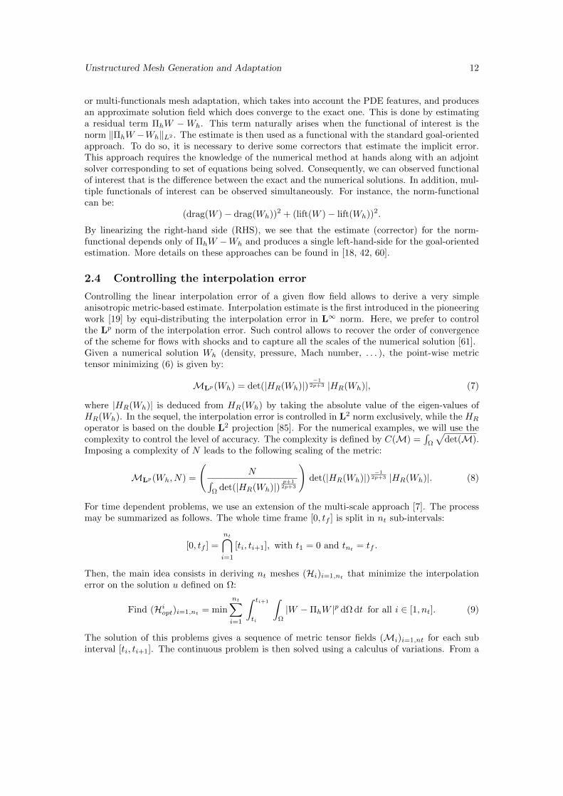
Unstructured Mesh Generation and Adaptation 12
or multi-functionals mesh adaptation, which takes into account the PDE features, and producesan approximate solution field which does converge to the exact one. This is done by estimatinga residual term ⇧
h
W � Wh
. This term naturally arises when the functional of interest is thenorm k⇧
h
W �Wh
kL
2 . The estimate is then used as a functional with the standard goal-orientedapproach. To do so, it is necessary to derive some correctors that estimate the implicit error.This approach requires the knowledge of the numerical method at hands along with an adjointsolver corresponding to set of equations being solved. Consequently, we can observed functionalof interest that is the di↵erence between the exact and the numerical solutions. In addition, mul-tiple functionals of interest can be observed simultaneously. For instance, the norm-functionalcan be:
(drag(W ) � drag(Wh
))2 + (lift(W ) � lift(Wh
))2.
By linearizing the right-hand side (RHS), we see that the estimate (corrector) for the norm-functional depends only of ⇧
h
W � Wh
and produces a single left-hand-side for the goal-orientedestimation. More details on these approaches can be found in [18, 42, 60].
2.4 Controlling the interpolation error
Controlling the linear interpolation error of a given flow field allows to derive a very simpleanisotropic metric-based estimate. Interpolation estimate is the first introduced in the pioneeringwork [19] by equi-distributing the interpolation error in L1 norm. Here, we prefer to controlthe Lp norm of the interpolation error. Such control allows to recover the order of convergenceof the scheme for flows with shocks and to capture all the scales of the numerical solution [61].Given a numerical solution W
h
(density, pressure, Mach number, . . . ), the point-wise metrictensor minimizing (6) is given by:
ML
p(Wh
) = det(|HR
(Wh
)|) �12p+3 |H
R
(Wh
)|, (7)
where |HR
(Wh
)| is deduced from HR
(Wh
) by taking the absolute value of the eigen-values ofH
R
(Wh
). In the sequel, the interpolation error is controlled in L2 norm exclusively, while the HR
operator is based on the double L2 projection [85]. For the numerical examples, we will use thecomplexity to control the level of accuracy. The complexity is defined by C(M) =
R⌦
pdet(M).
Imposing a complexity of N leads to the following scaling of the metric:
ML
p(Wh
, N) =
N
R⌦
det(|HR
(Wh
)|) p+12p+3
!det(|H
R
(Wh
)|) �12p+3 |H
R
(Wh
)|. (8)
For time dependent problems, we use an extension of the multi-scale approach [7]. The processmay be summarized as follows. The whole time frame [0, t
f
] is split in nt
sub-intervals:
[0, tf
] =nt\
i=1
[ti
, ti+1
], with t1
= 0 and tnt = t
f
.
Then, the main idea consists in deriving nt
meshes (Hi
)i=1,nt that minimize the interpolation
error on the solution u defined on ⌦:
Find (Hi
opt
)i=1,nt = min
ntX
i=1
Zti+1
ti
Z
⌦
|W � ⇧h
W |p d⌦ dt for all i 2 [1, nt
]. (9)
The solution of this problems gives a sequence of metric tensor fields (Mi
)i=1,nt
for each subinterval [t
i
, ti+1
]. The continuous problem is then solved using a calculus of variations. From a

Unstructured Mesh Generation and Adaptation 13
practical point of view, on a time interval [ti
, ti+1
], the flow solver outputs a sequence of solutionsevery �t = (t
i+1
� ti
)/N . From this sequence, a maximal or mean hessian Hi
is recovered [7]accounting for the error for the sub-window time frame. Then, once all H
i
are recovered, a globalnormalization is applied for the whole time frame [0, t
f
] to derive (Mi
)i=1,nt
, see Figure 26.
A detailed review of metric-based estimates for steady and unsteady problems can be foundin [6].
2.5 Geometric estimate for surfaces
Controlling the deviation to a surface has been studied in previous works, see [13, 28, 31] foranisotropic remeshing. We recall that the surface remeshing is done by considering only discretedata, either inherited by the CAD or recovered directly from the discrete mesh. Prior to surfaceremeshing, normals and tangents are then assigned to each boundary point. We denote by n
i
the normal of the vertex xi
. As in [28], a quadratic surface model is computed locally arounda surface point x
i
. Starting from the topological neighbors of xi
, the coordinates of each pointare mapped onto the local orthonormal Frenet frame (u
i
,vi
,ni
) centered in xi
. Vectors (ui
,vi
)lie in the orthogonal plane to n
i
. We denote by (uj
, vj
, �j
) = (txj
.ui
, txj
.vi
, txj
.ni
) the newcoordinates of vertex x
j
. xi
is set as the new origin so that (ui
, vi
, �i
) = (0, 0, 0). The surfacemodel consists in computing by a least squares approximation a quadratic surface:
�(u, v) = au2 + bv2 + cuv, where (a, b, c) 2 R3. (10)
The least squares problem gives the solution to min(a,b,c)
Pj
|�j
� �(uj
, vj
)|2, where j is the setof neighbors of x
i
. Note that 3 neighbors points are necessary to recover the surface model.Finally, if the degree of x
i
is d and the linear system is:
A X = B ()
0
B@u2
1
v2
1
u1
v1
......
...u2
d
v2
d
ud
vd
1
CA
0
@abc
1
A =
0
B@�
1
...�d
1
CA .
The least square formulation consists in solving tA A = tA B. From this point, one may appliedthe surface metric given in [28]. We propose here a simplified version. We can first remark thatthe orthogonal distance from the plane n?
i
onto the surface is given by �(u, v) by definition.The trace of �(u, v) on n?
i
is a function that gives directly the distance to the surface. The2D surface metric M2D
S
such that the length `M2DS
((u, v)) is constant equal to " is easy to findstarting from the diagonalization of the quadratic function (10). Geometrically, it consists infinding the maximal area metric included in the level-set " of the distance map. We assume thatM2D
S
admits the following decomposition:
M2D
S
= (uS
, vS
)
✓�
1,S
00 �
2,S
◆t(u
S
, vS
), with (uS
, vS
) 2 R2⇥2.
If we want to achieve the same error as the initial mesh, we compute " = minj
|�(uj
, vj
)| amongthe neighbors of x
i
. The anisotropic 2D metric achieving an " error becomes:
M2D
S
(") =1
"M2D
S
.

Unstructured Mesh Generation and Adaptation 14
The final 3D surface metric in xi
is:
MS
(") = (uS
,vS
,ni
)
0
BBBB@
�1,S
"0
0�
2,S
"0
0 0 h�2
max
1
CCCCAt(u
S
,vS
,ni
), (11)
with
(uS
= uS
(1)ui
+ uS
(2)vi
,
vS
= vS
(1)ui
+ vS
(2)vi
.
The parameter hmax
is initially chosen very large (e.g. 1/10 of the domain size). This normal sizeis corrected during various steps. A first anisotropic gradation using (4)(i) is applied on surfaceedges only. The surface metric is then intersected with any computation metrics as given by (7).These two steps set automatically a proper element size in the normal direction. Note di↵erentlocal surface estimates can be derived depending on the local information available, see [88].
During the mesh adaptation process, the previous procedure is not applied independently oneach current mesh to be adapted. On the contrary, the surface metric is computed once on afixed background mesh. This metric is then interpolated on each adapted mesh in the course ofthe iterative process. This tends to maintain a consistent gap with respect to the true geometry.
2.6 Boundary layers metric
Boundary layers mesh generation has been devised to capture accurately the speed profile arounda body during a viscous simulation. The width of the boundary layer depends on the localreynolds number [53]. So far, the generation of the boundary layer grids has been carried outby an extrusion of the initial surface along the normals to the surface or by local modification ofthe mesh [68]. Note that using the normals as sole information requires several enrichments toobtain a smooth layers transition on complex surfaces [14]. In this chapter, we consider a simpleapproach that is naturally compatible with anisotropic adaptation procedures. The idea consistsin representing the boundary layer mesh by a continuous metric field.
The distance to the body is computed using classical algorithms of level-set methods [53].This step can be done quickly and has generally a complexity of O(N ln(N)) where N is thenumber of points in the current mesh. (Furthermore, note that from a practical point of view,this function is evaluated only in the vicinity of the body). To control the size in the tangentialdirections, a metric is recovered from the current surface mesh or a background mesh. It takesadvantage of the Log-Euclidean framework. Starting from an elements (K)
P2K
of vertex P , theunique surface metric tensor M
K
(for which K is unit) is computed by solving the following6 ⇥ 6 linear system:
(S)
8<
:
`2MK(e
1
) = 1. . .`2MK
(e6
) = 1 .(12)
where (ei
)i=1,6
are elements edges. (S) has a unique solution as long as the volume of K is notnull. The logarithm of each metric is computed so that a classical Euclidean mean weightedby the elements’ area is done. Finally, the body point metric M
P
is mapped back using theexponential operator:
MP
= exp
✓PP2K
|K| ln(MK
)PP2K
|K|◆
.

Unstructured Mesh Generation and Adaptation 15
The final boundary layers metric is based for a continuous exponential law of the form h0
exp(↵�(.)),where h
0
is the initial boundary layer size and ↵ the growing factor. For a volume point xi
, theboundary layers metric depends on the body point P
i
for which the minimum distance is reached.The following operations conclude this step:
1. Compute the local Frenet frame (ui
,vi
, r�(xi
)) associated with r�(xi
)
2. Set the size in the normal direction to hni = h
0
exp(↵ �(xi
)), the sizes in the orthogonalplane to:
hui = (tu
i
MPi ui
)�2
and hvi = (tv
i
MPi vi
)�2
,
3. The final metric is given by:
Mbl
(xi
) = t(ui
,vi
, r�(xi
))
0
@h�2
ui
h�2
vi
h�2
ni
1
A (ui
,vi
, r�(xi
)). (13)
The key idea is again to simplify the coupling by using only metric tensor fields. Indeed,taking all together the viscous and un-viscous contributions simply consist in intersecting thecorresponding metric tensor fields.
3 Algorithms for generating anisotropic meshes
This section describes the local operators used to adapt the mesh once one or several tensor fieldsare provided on input. We then describe additional operators used to optimize the mesh and toguarantee an optimal time step for unsteady simulations.
3.1 Insertion and collapse
To generate a unit-mesh in a given metric field (Mi
)i=1...N
, two operations are recursively used:edge collapse and point insertion on edge.The starting point for the insertion of a new point on an edge e is the shell of e composed of allelements sharing this edge. Each element of the shell is then divided into two new elements. Thenew point is accepted if each new tetrahedron has a positive volume. When a point is insertedon an boundary edge, either a linear approximation of the surface is used or a query to the CAD.The newly inserted point is created at the mid-edge point in the metric. To compute it, we firstevaluate the size of the current edge with respect to the two end-points (A, M
A
) and (B, MB
):
`MA =p
tAB MA
AB and `MB =p
tAB MB
AB.
If `MA equals `MB , the mid-edge point in the metric is the geometric mid-point 1
2
(A + B).When they di↵er, we need to solve the non-linear problem in t 2 [0, 1] arising for the lengthapproximation of (1):
Find t such that1
2= `MA
rt � 1
log(r)with r =
`MB
`MA
. (14)
We use a dichotomy approach to solve (14), the mid-point is then (1 � t) A + t B.The edge collapse starts from the ball of the vertex to be deleted. Again, for the deletion ofpoints inside the volume, the only possible rejection is the creation of a negative volume element.A special care is also required to avoid the creation of an element that already exists, see Figure 9
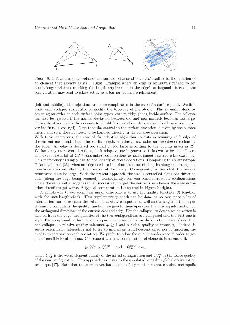
Unstructured Mesh Generation and Adaptation 16
AB
Volume case Surface case
A
B
Merging A onto B
Figure 9: Left and middle, volume and surface collapse of edge AB leading to the creation ofan element that already exists . Right, Example where an edge is recursively refined to geta unit-length without checking the length requirement in the edge’s orthogonal direction; theconfiguration may lead to edges acting as a barrier for future refinement.
(left and middle). The rejections are more complicated in the case of a surface point. We firstavoid each collapse susceptible to modify the topology of the object. This is simply done byassigning an order on each surface point types: corner, ridge (line), inside surface. The collapsecan also be rejected if the normal deviation between old and new normals becomes too large.Currently, if n denotes the normals to an old face, we allow the collapse if each new normal n
i
verifies tnni
> cos(⇡/4). Note that the control to the surface deviation is given by the surfacemetric and so it does not need to be handled directly in the collapse operation.With these operations, the core of the adaptive algorithm consists in scanning each edge ofthe current mesh and, depending on its length, creating a new point on the edge or collapsingthe edge. An edge is declared too small or too large according to the bounds given in (2).Without any more considerations, such adaptive mesh generator is known to be not e�cientand to require a lot of CPU consuming optimizations as point smoothing and edge swapping.This ine�ciency is simply due to the locality of these operations. Comparing to an anisotropicDelaunay kernel [25], when an edge needs to be refined, the metric lengths along the orthogonaldirections are controlled by the creation of the cavity. Consequently, in one shot, the area ofrefinement must be large. With the present approach, the size is controlled along one directiononly (along the edge being scanned). Consequently, one can reach intractable configurationswhere the same initial edge is refined successively to get the desired size whereas the sizes in theother directions get worse. A typical configuration is depicted in Figure 9 (right).
A simple way to overcome this major drawback is to use the quality function (3) togetherwith the unit-length check. This supplementary check can be done at no cost since a lot ofinformation can be re-used: the volume is already computed, as well as the length of the edges.By simply computing the quality function, we give to these operators the missing information onthe orthogonal directions of the current scanned edge. For the collapse, to decide which vertex isdeleted from the edge, the qualities of the two configurations are compared and the best one iskept. For an optimal performance, two parameters are added in the rejection cases of insertionand collapse: a relative quality tolerance q
r
� 1 and a global quality tolerance qa
. Indeed, itseems particularly interesting not to try to implement a full descent direction by imposing thequality to increase on each operation. We prefer to allow the quality to decrease in order to getout of possible local minima. Consequently, a new configuration of elements is accepted if:
qr
Qini
M Qnew
M and Qnew
M < qa
,
where Qini
M is the worse element quality of the initial configuration and Qnew
M is the worse qualityof the new configuration. This approach is similar to the simulated annealing global optimizationtechnique [47]. Note that the current version does not fully implement the classical metropolis

Unstructured Mesh Generation and Adaptation 17
algorithm where the rejection is based on a random probability. To ensure the convergence ofthe algorithm, the relative tolerance q
r
is decreased down to 1 after each pass of insertions andcollapses. At the end of the process, the absolute tolerance q
a
is set up to the current worsequality among all elements.
3.2 Optimizations and enhancement for unsteady simulations
In addition to the quality-driven insertion and collapse, we use standard anisotropic mesh opti-mization techniques such as edges and faces swaps and point smoothing in order to increase thelevel of anisotropy and the quality of the mesh. By improving the overall quality, they usuallyimprove the stability of the flow solver as well. For unsteady simulations, we add an additionalcontrol parameter in order to ensure that an optimal time step is provided in the adaptive mesh.
Swaps of edges and faces are standard mesh modifications operators, see [27, 32]. In the con-text of anisotropic remeshing, theses operators are simply monitored by anisotropic quality (3).Once the topological and geometrical validity of a swap is verified (positive volume and valid newconfigurations), it is actually performed only if the quality of the new configuration is strictlylower that the initial quality. We use an improvement factor q
r
= 0.95 for all the numericalexamples.
The point smoothing is also a popular simple operator [32]. It consists in computing a newoptimal position of a vertex to improve the quality of the surrounding elements. The maindi�culty is the computation of the optimal position. In our case, we want to optimize the lengthdistribution as well. Consequently, for an edge PP
i
with metric M(P ) and M(Pi
), the optimalpoint position of P is approximated in a Riemannian way by computing :
✓ = 1 � log
✓`M(P )
`M(P ) � log(r)
◆1
log(r)with
8<
:
`M(P ) =p
PPi
M(P )PPi
,`M(P
i
) =p
PPi
M(Pi
)PPi
,r = `M(P )/`M(P
i
).
The formula arises from seeking the optimal size to get a unit-edge length along PPi
:
Z✓
0
`M(P )t�1`M(Pi
)�tdt = 1.
Then the optimal position for P from Pi
is :
Popti = P + ✓ P
i
P.
This procedure is repeated with all the neighboring vertices of P :
Popt
= ↵P +1 � ↵
nP
nPX
i=1
Popti
!with ↵ 2 [0, 1]
If Popt
generates positive volume elements and improves the final quality, P is moved to this newposition. In case of rejection, a greater value of ↵ is considered starting with ↵ = 0.2. Note thatthe metric of P is interpolated at the new position to evaluate the new quality. When a surfacepoint is moved, it is also projected back to the surface and the surface deviation is check in asimilar way as for the insertion and collapse operators.
For unsteady simulations, the mesh adaptation becomes critical as the CPU time of thesimulation depends on the quality of the worse element. Indeed, when an explicit time steppingis used, the minimal time step governs the speed of the simulation. Consequently, the minimalsize (or height) generated during the remeshing process may impact drastically the CPU time.

Unstructured Mesh Generation and Adaptation 18
If the generated size if 0.01 of the minimal target, then the while CPU time will be multipliedby 100. To overcome this issue, we add an additional control to the quality based on the heightof the tetrahedra. We start from the definition of the minimal height of a tetrahedron:
h2 =1
3
V
Smax
, (15)
where h is the minimal height, V the volume and Smax
the maximal area of the faces. For eachprovided metric, we consider then the regular tetrahedron of side h
1
, h2
, h3
, where (hi
)i
are theunit lengths along the eigenvectors of the metric. Then, assuming that the sizes may be in therange [ 1p
2
hi
,p
2hi
], see (2), we can estimate the global minimal height htar
using (15). A mesh
modification is then rejected if the minimal height of the new set of tetrahedra is lower thanhtar
and the minimal height of the initial set of elements. Numerical experiments have proventhat this additional constraint does not have a negative impact on the level of anisotropy whilepreserving an optimal CPU time step.
4 Adaptive algorithm and numerical illustrations
The previous mesh adaptation strategy is used inside an adaptive loop that couples the errorestimations, the mesh adaptation and the flow solver. In this section, we give some additionaldetails on the components that are not relative to the local remeshing. We then first validatethe full adaptive approach on a supersonic wing-body configuration and a transonic ONERA m6wing. For each case, the adapted numerical solution is compared with experiments. Then, weconsider the direct sonic boom prediction of a complex aircraft. The adaptive strategy is thenapplied to the prediction of boundary layer/shock interaction. Finally, we consider unsteadysimulations with the double Mach reflection and a blast prediction.
4.1 Adaptive loop
The complete adaptive algorithm for steady simulations is composed of the following steps.
1. Compute the flow field (i.e. converge the flow solution on the current mesh);
2. Compute the metric estimates: surface, volume, boundary layers, etc.
3. Generate a unit mesh with respect to these metric fields;
4. Re-project the surface mesh onto the geometry using the CAD data or a fixed backgroundmesh;
5. Interpolate the flow solution on the new adapted mesh;
6. Goto 1.
For Step 1., two flow solvers have been used in the numerical section. The first one, FEFLO [53],works on unstructured grids with finite element discretization of space and edge-based datastructures. The Galerkin edge-fluxes are replaced by numerically consistent fluxes, typically givenby approximate Riemann solvers (van Leer, Roe, HLLC, ...) with limited variables (van Leer, vanAlbada, ...). The second flow solver is WOLF [5] and it uses a mixed Finite Element/Finite Volumediscretization with a MUSCL extrapolation. Both codes have been verified to be second orderaccurate on smooth flows and second order accurate for flows with shocks by using adaptivity [61,62]. The flow solvers use an implicit LU-SGS scheme [66, 71]. FEFLO is used for simulations 4.4

Unstructured Mesh Generation and Adaptation 19
and 4.5, WOLF for simulations 4.2, 4.3 and 4.6. For the unsteady simulations, an explicit timestepping based on Runge-Kutta schemes is used and the explicit control of the height of thetetrahedra of Section 3.2 is activated.
For Step 4., if the surface approximation " is small enough with respect to the minimalmetric size controlling the interpolation error, the simple smoothing procedure usually succeeds todirectly move the point onto the geometry. For more complex cases, with boundary layer or whenthe surface approximation is low, most advanced operators like the cavity-based operators [64]are needed.
For all the simulations, we use a 8-processors 64-bits MacPro with an IntelCore2 chipsetswith a clockspeed of 2.8GHz with 32Gb of RAM. The flow solver is multi-threaded while thelocal remeshing is serial. The final metric field (multi-scale, surface, boundary-layer) is alwayssmoothed by using isotropic gradation law (4)(i), with a parameter of 1.2.
To evaluate the level of anisotropy, we use the anisotropic ratio and anisotropic quotients ofan element. Both measures are uniquely defined by computing the metric solution of (12), and
then by evaluating the following quantities from its eigenvalues with hi
= �� 1
2i
:
r =max
i=1,3
hi
mini=1,3
hi
and qi
=h3
i
h1
h2
h3
Anisotropic quotients measure the gain with respect to an isotropic mesh adaptation, in partic-ular, they increase when two anisotropic directions exist.
For all cases, the initial meshes are generated by using either a constrained Delaunay approachfor simulations 4.2 and 4.3 and a frontal approach for simulations 4.4, 4.5 and 4.6. Note thatonly the material described in the previous sections are used. The interpolation error in L2 normis used in addition to the surface metric, metric smoothing and boundary layer metric describedin Section 2. The algorithm used to generate the meshes exactly fits the procedures given inSection 3.
4.2 A wing-body configuration
The first example is a supersonic flows around the 4th wing-body configuration described in [67].The planform of the model and the corresponding CAD are depicted in Figure 10. The inflowis a at Mach 1.68 with a lift of 0.15. We observe the pressure below the aircraft at a distanceR = 3.1 L where L is the reference length of the aircraft (here 17.52 cm). Experimental dataare available at this distance, see [67]. The adaptive process is based on metric (7) coupled withthe surface metric (11) with " = 0.001. The simulation is composed of 3 steps at the followingcomplexity : 25 000, 50 000 and 75 000 with 5 sub-iterations at a fixed complexity yielding toa total of 15 iterations. We control the interpolation error of the Mach number in L2 norm.The final mesh is here composed of 283 625 vertices and 1 582 309 tetrahedra. The worst volumequality is 0.05 and the worst surface quality is 0.11 The average anisotropic ratio is 61 and themean anisotropic quotient is 2711. 92 % and 99.9 % of the volume and surface edges respectivelyare unit. The total CPU time for this run is 61 mn. This case features 3 strong shocks that arewell and early captured by the adaptive process, see Figure 11 for comparisons with experiments.
4.3 Transonic flow around a M6 wing
We consider a flow around the Onera-M6 wing. The initial surface mesh and the CAD aredepicted in Figure 12. The flow condition is Mach 0.8395 with an angle of attack of 3.06 degrees.The scope of the example is to validate the interaction between the surface metric controlledwith " = 0.001 and the Lp metric. For this simulation, the following sequence of complexities

Unstructured Mesh Generation and Adaptation 20
7.01
8.21
16.29
17.52
3.45
1.2369º
80º
x
r
0.54
c
c/2
t t/2
t/c=0.05
Figure 10: Wing-body example: Left, planform of the wing-body model. Right, CAD of themodel equipped with a parabolic sting to emulate experiment apparatus.
0 0.5 1 1.5−0.03
−0.02
−0.01
0
0.01
0.02
0.03
ite.15: 183K
ite.10: 194K
ite.5: 106K
XP
Figure 11: Wing-body example: Left, normalized pressure signature p�p1p1
at R/L = 3.6 for thefinal meshes for each fixed complexity. Right, closer view of the final anisotropic adaptive meshnear the observation line.
for (8) is chosen: 20 000, 40 000 and 80 000, with 5 steps at a fixed complexity. The L2 norm ofthe interpolation error of the Mach number is controlled. The final mesh is composed of 222 561vertices and 1 247 227 tetrahedra with a mean anisotropic ratio of 43 and a mean anisotropicquotient of 1662. The total CPU time for this simulation is 42 mn, with 55 % spent in the flowsolver and 45 % in the remeshing, interpolation and error estimate. For the final mesh, the worstquality is 0.11 for the volume and 0.25 for the surface. The strong shocks on the surface of thewing are depicted in Figure 13. C
p
extractions along two sections are given in Figure 15. InFigure 14, we observe the anisotropic volume meshes near the wake of the wing and near theshocks on the wing surface. Note that if the shock-dominated features of the flow are perfectlycaptured, we also capture smooth features as the wing tip vortex, see Figure 16. The amplitudeof the flow variables in the wake are 2 orders of magnitude lower than the magnitude in theshock.
4.4 Direct sonic boom simulation
We consider in this example the accurate prediction of the pressure signal below the SSBJ designprovided by Dassault-Aviation. The length of the aircraft is L = 43 m while the distance ofobservation from the aircraft is denoted by R. The initial surface mesh is depicted in Figure 17.The aircraft is put in a 10 km domain as depicted in Figure 17 (right). The initial mesh wasgenerated automatically by using an advancing-front technique [55]. The size ratio in the initial

Unstructured Mesh Generation and Adaptation 21
Figure 12: M6 wing example: Left, CAD of the geometry, right, a view of the initial surfacemesh of the wing.
Figure 13: M6 wing example: From left to right, anisotropic surface mesh, Mach iso-values,closer view near the second shock.
Figure 14: M6 wing example: From left to right, anisotropic capturing of the wake and of theshock, closer view in the wake, closer view around the shock.
0 0.1 0.2 0.3 0.4 0.5 0.6 0.7−0.8
−0.6
−0.4
−0.2
0
0.2
0.4
0.6
0.8
1
1.2
ite.15: 222K
XP
0 0.1 0.2 0.3 0.4 0.5 0.6 0.7−0.8
−0.6
−0.4
−0.2
0
0.2
0.4
0.6
0.8
1
1.2
ite.15: 222K
XP
Figure 15: M6 wing example: Left and middle, comparisons between experimental values ofC
p
= (p � p1)/q1 for the second and third upper sections of the wing. Right, closer view of themesh near upper sections 2 and 3.

Unstructured Mesh Generation and Adaptation 22
Figure 16: M6 wing example: Wing tip vortex 8 body-length behind the wing.
10km
15km
Figure 17: SSBJ example: Left, initial surface mesh of the SSBJ geometry, right, computationaldomain with the position of the aircraft in the domain.
mesh is hmin
/hmax
= 1e�9 and the volume of the elements ranges from 5.4e�11 to 4.7e10. Theflow condition is Mach number 1.6 with an angle of attack of 3 degrees. Our intent is to observedthe pressure field for various R up to 9 km. This corresponds to a ratio R/L of about 243.According to the flow conditions, for R = 9 km, the length of the propagation of the shock wavesemitted by the SSBJ is actually around 15 km.
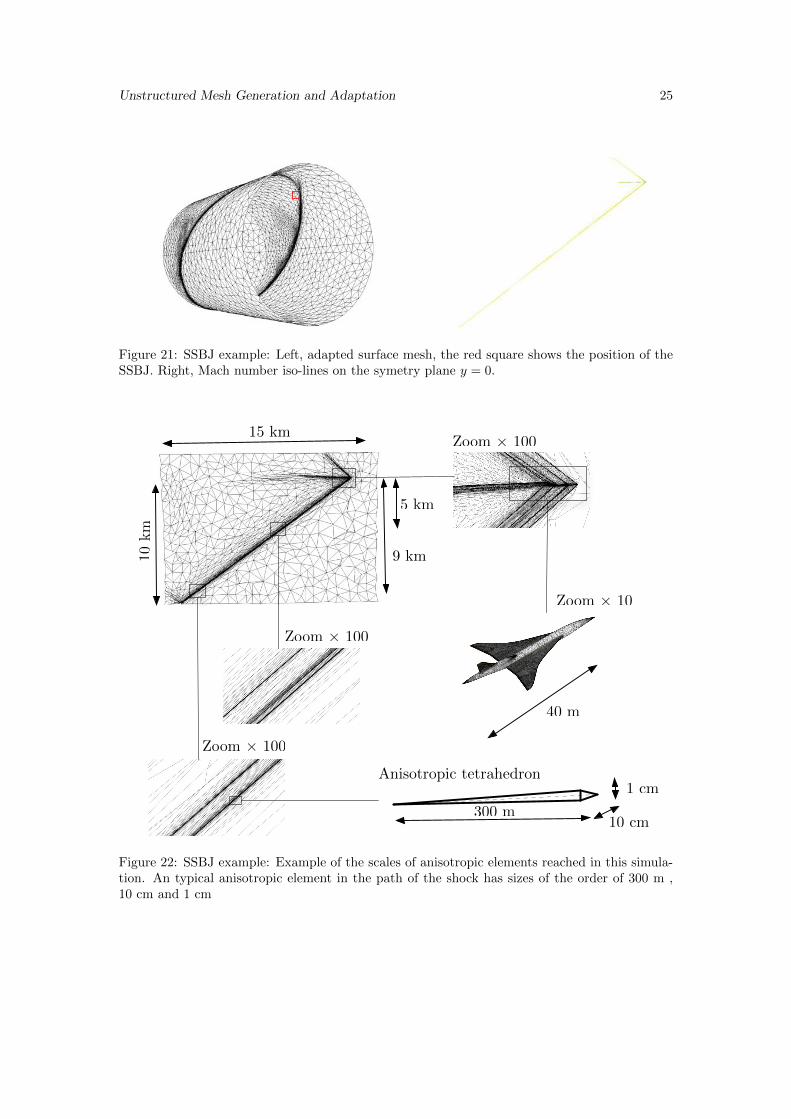
The interpolation error on the Mach number in L2 norm is controlled and the surface iscontrolled with (11) and " = 0.001. The strategy employed here is based on 30 adaptations atthe following complexities: 80 000 , 160 000, 240 000, 400 000, 600 000 and 800 000. Each stepis composed of 5 sub-iterations at a fixed complexity. The final mesh is composed of 3 299 367vertices and 19 264 402 tetrahedra only. The average anisotropic ratio is 1907 while the meananisotropic quotient is 50 3334. All the scales involved in this simulation are depicted in Figure 22.This example shows that a very high level of anisotropy is reached using unstructured meshadaptation. Indeed, it is at least one order of magnitude higher than in the previous examples.Local refinement allows to keep a maximum accuracy and enables to generate quality anisotropicmeshes. We mention that for each generated mesh, the worst element quality computed with (3)is always below 0.02 for the volume and below 0.05 for the surface while the percentage of unitelements is always greater than 90 %. In addition, the flow solver still converges on such meshesleading to accurate pressure signatures for R/L ⇡ 250. Anisotropic ratios and quotients for thewhole sequence of meshes are reported in Table 1. They are increasing along the iterations.This shows that the accuracy across the shocks is increasing while the sizes in the anisotropic

Unstructured Mesh Generation and Adaptation 23
Table 1: SSBJ example: Properties of each final adapted mesh : mean anisotropic ratio, meananisotropic quotient, number of vertices and number of tetrahedra for each complexity. The lastcolumn gives the cumulative CPU time.
Iteration Complexity Ratio Quotient # Vertices # Tet. CPU time
5 80 000 200 10 964 432 454 2 254 826 1 h 10 mn
10 160 000 383 30 295 608 369 3 294 197 2 h 54 mn
15 240 000 698 81 129 1 104 910 6 243 462 6 h 9 mn
20 400 000 1 089 177 295 1 757 865 10 125 724 11 h 15 mn
25 600 000 1 575 340 938 2 572 814 14 967 820 18 h 47 mn
30 800 000 1 907 503 334 3 299 367 19 264 402 28 h 35 mn
Figure 18: SSBJ example: Left, cut in the final adapted mesh 10 m below the aircraft. Right, cut10 m behind the aircraft showing how anisotropic tetrahedra are aligned with the Mach cones.
directions are decreasing at a lower rate. The fact that the anisotropic quotient is increasingsimply shows that there exist two anisotropic directions. Note that using (7) avoid to prescribea minimal size during the adaptation leading to even stronger anisotropy. This property is
due to the sensitivity property of (7) given by the local normalization term det(|HR
(uh
)|) �12p+3 .
An example of the scales of the solution is given by the pressure extractions in Figure 20 atR = 5 km and R = 9 km. Indeed, the normalized pressure signal at R = 9 km is of order8e�4 while the magnitude is around 3e�2 at R = 43 m. Consequently, we can expect for thevolume interpolation error to have a magnitude ratio of (102)3. It is then necessary to guaranteethat the error estimate detects such small amplitudes even in the presence of large amplitudes.This example demonstrates that using (7) complies with this requirement allowing to detectautomatically all the scales of the solution, see Figure 20. Several cuts in the symmetry planeare depicted in Figure 19. At R = 5 km, we still distinguish 3 separated shocks waves and atR = 9 km only two shock waves are separated leading the classical N-wave signature. Thesefeatures are even more emphasized on the pressure signatures in Figure 20.
The total CPU time is around 28 h 35 mn. 75 % of the CPU time is spent in the flow solverand 35 % in the remeshing, interpolation and error estimate. Note that accurate signaturesat R = 5 km are already obtained after 11 h of CPU (corresponding to the 20th iteration) asdepicted in Figure 20. We give in Table 1 the full sequence of CPU times. The first three stepsprovides an accurate signal for R/L < 20 and below.
4.5 Boundary layer shock interaction
We apply this strategy to study shock/boundary layer interaction. The test case is depictedin Figure 23. The shock waves are generated by a double wedge wing at Mach 1.4 with anangle attack of 0 degree and a Reynolds number of 3.4 106. Only the plate is treated as aviscous body. We solve the set of the Reynolds-average Navier-Stokes equations with BaldwinLomax turbulence model. The final adapted mesh and the Mach number iso-values are depicted

Unstructured Mesh Generation and Adaptation 24
R = 5 km
R = 9 km
Figure 19: SSBJ example: From top to bottom, from left to rigth, cut in the final anisotropicmesh close to the aircraft, closer view of the mesh 5 km below the aircraft, closer view at 9 kmbelow the aircraft, global view of the mesh.
500 1000 1500 2000 2500 3000 3500 4000 4500 5000 5500 6000−8
−6
−4
−2
0
2
4
6
8
10
x
(p−
p!
)/p!
x 1
0−
4
ite.20: 1M7
ite.25: 2M5
ite.30: 3M3
0 1000 2000 3000 4000 5000 6000−1.5
−1
−0.5
0
0.5
1
1.5
x
(p−
p!
)/p!
x 1
0−
3
ite.20: 1M7
ite.25: 2M5
ite.30: 3M3
R = 9 km R = 5 km
Figure 20: SSBJ example: Left, pressure signature at R = 9 km for the final meshes correspond-ing the last three complexities. Right, pressure signature at R = 5 km. The legend reports thenumber of vertices of each mesh in million (Iteration 20, 25 and 30). The pressure curves aredeliberately shifted for visibility.
Unstructured Mesh Generation and Adaptation 25
Figure 21: SSBJ example: Left, adapted surface mesh, the red square shows the position of theSSBJ. Right, Mach number iso-lines on the symetry plane y = 0.
Zoom ⇥ 10
Zoom ⇥ 100
Zoom ⇥ 100
300 m10 cm
1 cm
Zoom ⇥ 100
40 m
5 km
9 km10km
15 km
Anisotropic tetrahedron
Figure 22: SSBJ example: Example of the scales of anisotropic elements reached in this simula-tion. An typical anisotropic element in the path of the shock has sizes of the order of 300 m ,10 cm and 1 cm

Unstructured Mesh Generation and Adaptation 26
Figure 23: Shock/boundary layer interaction example: from left to right, computational domainand initial surface mesh
in Figure 23, closer views around the two shocks are depicted in Figure 24. The final meshis composed of 280 000 vertices and 1.3 millions tetrahedra and is obtained after 20 iterationswith a complexity of 10 000. In this example, we control the interpolation error on the Machnumber coupled with boundary layer metric (13). The initial mesh is used as the backgroundmesh to compute (13) with parameters h
0
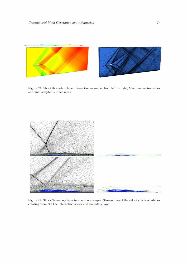
= 10�6 and ↵ = 1.2. As the boundary-layer metricis intersected with the interpolation error based metric, the resulting complexity is naturallygreater. The unstructured boundary layer mesh height is around 10�7 near the plate. Theaverage anisotropic ratio is grater than 106 and the average ratio around 500. The worst surfaceelement quality is 0.03 and 0.002 for the volume. For the final mesh, the minimal size in theunstructured layer is of the order of 10�7. As shown in Figure 24 (bottom), we successfullycapture the typical bubbles and re-circulations at the intersection between the shocks and theboundary layer.
This simulation leads to the following observations. Generating a semi-structured boundarylayer mesh extruded from the surface mesh gives only the require accuracy for the smaller layers.Indeed, the distance of the bottom of the shock from the viscous plate is around 10�3 whereasthe initial height of the uniform boundary layer mesh was at 0.2. Consequently, the example em-phasizes the di�culty of capturing these phenomena only with a an priori fixed quasi-structuredboundary layer mesh. In addition, this approach is completely generic and robust and can handlecomplex geometries. However, if the shock/boundary layer interaction is automatically handled,the impact of having a fully unstructured mesh is not yet analyzed in term of solution accu-racy and solver stability in the viscous area. Consequently, it seems also interesting to derivea method to generate structured mesh for the smaller layers (at least) while preserving (upper)anisotropic refinements. Metric-orthogonal and metric-aligned anisotropic mesh adaptation arepossible solutions to generate highly anisotropic meshes whith quasi-structured elements [56, 63].
4.6 Double Mach reflection and blast prediction
The first unsteady case is double Mach reflection. This simulation starts from a 2-state initial-ization of a shock wave impacting a ramp. The density, speed and pressure for the right side is(5.71, 9.76, 0, 0, 116.5) and (1, 0, 0, 0, 1) for the left side, the shock wave propagates along the x-direction. The total physical time of the simulation is 0.18s. For this simulation, the time frame[0, 0.18] is divided in 30 sub-time windows with 5 fixed point iterations and 21 metric intersec-tions for each sub-time window. We control the L2 norm of the density interpolation error. Thesimulation CPU time is 8h55m, 80% is spent in the flow solver and 20% mesh adaptation. The
Unstructured Mesh Generation and Adaptation 27
Figure 24: Shock/boundary layer interaction example: from left to right, Mach umber iso valuesand final adapted surface mesh.
Figure 25: Shock/boundary layer interaction example: Stream lines of the velocity in two bubblescreating from the the interaction shock and boundary layer.

Unstructured Mesh Generation and Adaptation 28
t
Tini
metric sampling
�T
�t
Tend
Fixed-point loop
Figure 26: Unsteady adaptation algorithm: a fixed mesh is generated for sub-time window bysampling the solution at di↵erent time steps.
final mesh is composed of 235 095 vertices, 1 310 082 tetrahedra and 5 864 boundary faces. Themesh at final time and density iso-values are depicted in Figure 27. We can see that the contactdiscontinuity is impacting the ramp and that the generated vortices are pushing forward theinitial front shock. If this phenomenon is usually observed in 2D simulation [89], its observationon 3D geometry is more complex. Moreover, the thickness of the adaptation is due to the fixedpoint strategy as the mesh is adapted for all the times step belonging to a sub-time frame.
We then consider a blast propagation on a more complex geometry: the US Capitol. Applyingsuccessfully an anisotropic adaptive simulation on it is challenging as it features many complexdetails as many columns, cupola, . . . . A classic load is considered, see Figure 28. The finalphysical time is 0.1 s. The whole time frame has been divided into 20 time slots of 0.005 s. Theflow solver outputs density field every 0.0005 s. The final anisotropic mesh for the time frame[0.05, 0.055] is depicted in Figure 28. The interpolation error on the density is controlled in L2
norm in space and time. The mesh is composed of almost 200 000 vertices for a total CPU timeof 8 hours.
5 Conclusion
The standard computational pipeline have been described for complex geometries and unstruc-tured mesh generation from CAD to surface and volume mesh generation. For adaptivity, wehave described the basic principles of anisotropic mesh adaptation based on metric tensor fields:concept of unit mesh, metric interpolation, metric smoothing, . . . A simple to implement butrobust local remeshing strategy have been detailed. It allows to adapt di↵erent components ofthe flows. For each adaptation, we use a dedicated metric field issued from various estimates:surface curvatures, interpolation errors, distance to a body, . . . Numerical examples show therobustness of the method to (i) reduce solver di↵usion and (ii) reach a high level of anisotropythat is hardly tractable with a structured approach or a global remeshing method.
This chapter has covered only the basic processes that are required to reach a high level ofanisotropy and recover a second order accuracy in space when simulating flows with shocks. Itis important to mention that each component is crucial to gain all the benefit of adaptivity.Any improvement in one component may improve the whole process. We refer to [75] for adetailed discussion on the current issues of unstructured mesh adaptation. Mesh generation andadaptation is still an active field of research and many topics are not discussed in this chapter.This concerns the generation of boundary layer grids [14, 17, 33], the design of metric-aligned ormetric-orthogonal grids [56, 63], the design of very high-order error estimates [91], the generation

Unstructured Mesh Generation and Adaptation 29
3D Double Mach Reflection
Mesh size: 235 095 vertices, 1 310 082 tetrahedra and 57 864boundary faces
87 Anisotropic Mesh Adaptation for CFD
3D Double Mach Reflection
Mesh size: 235 095 vertices, 1 310 082 tetrahedra and 57 864boundary faces
87 Anisotropic Mesh Adaptation for CFD
3D Double Mach Reflection
Mesh size: 235 095 vertices, 1 310 082 tetrahedra and 57 864boundary faces
87 Anisotropic Mesh Adaptation for CFD
3D Double Mach Reflection
Mesh size: 235 095 vertices, 1 310 082 tetrahedra and 57 864boundary faces
87 Anisotropic Mesh Adaptation for CFDFigure 27: Double Mach reflection at final time : final adapted surface mesh (top left), densityiso-values (top right), cut in the volume mesh (bottom left) and closer view near the contactdiscontinuity and vortex shock interaction (bottom right).

Unstructured Mesh Generation and Adaptation 30
Figure 28: Top, the US capitol CAD (left) and initial surface mesh (right) with the initial blastlocation. Bottom, anisotropic surface mesh at t = 0.025s (left) and the density solution iso-values(right).
of high-order curved meshes [3, 80, 84, 90] and parallel (adaptive) mesh generation [9, 23, 65,73, 78].
References
[1] R. Abgrall, Toward the ultimate conservative scheme: Following the quest, Journal ofComputational Physics, 167 (2001), pp. 277 – 315.
[2] R. Abgrall, H. Beaugendre, and C. Dobrzynski, An immersed boundary methodusing unstructured anisotropic mesh adaptation combined with level-sets and penalizationtechniques, Journal of Computational Physics, 257, Part A (2014), pp. 83 – 101.
[3] R. Abgrall, C. Dobrzynski, and A. Froehly, A method for computing curved meshesvia the linear elasticity analogy, application to fluid dynamics problems, International Jour-nal for Numerical Methods in Fluids, 76 (2014), pp. 246–266.
[4] F. Alauzet, Size gradation control of anisotropic meshes, Finite Elements in Analysis andDesign, (2009). published online.
[5] F. Alauzet and A. Loseille, High order sonic boom modeling by adaptive methods, J.Comp. Phys., 229 (2010), pp. 561–593.
[6] F. Alauzet and A. Loseille, A decade of progress on anisotropic mesh adaptation forcomputational fluid dynamics, Computer-Aided Design, 72 (2016), pp. 13 – 39. 23rd Inter-national Meshing Roundtable Special Issue: Advances in Mesh Generation.
Unstructured Mesh Generation and Adaptation 31
[7] F. Alauzet and G. Olivier, Extension of Metric-Based Anisotropic Mesh Adaptation toTime-Dependent Problems Involving Moving Geometries, American Institute of Aeronauticsand Astronautics, 2014/03/26 2011.
[8] A. Alleaume, Automatic Non-manifold Topology Recovery and Geometry Noise Removal,Springer Berlin Heidelberg, Berlin, Heidelberg, 2009, pp. 267–279.
[9] A. Alleaume, L. Francez, M. Loriot, and N. Maman, Automatic tetrahedral out-of-core meshing, Springer Berlin Heidelberg, Berlin, Heidelberg, 2008, pp. 461–476.
[10] V. Arsigny, P. Fillard, X. Pennec, and N. Ayache, Log-Euclidean metrics forfast and simple calculus on di↵usion tensors, Magnetic Resonance in Medicine, 56 (2006),pp. 411–421.
[11] R. Aubry, S. Dey, K. Karamete, and E. Mestreau, Smooth anisotropic sources withapplication to three-dimensional surface mesh generation, Engineering with Computers, 32(2016), pp. 313–330.
[12] R. Aubry, S. Dey, E. Mestreau, B. Karamete, and D. Gayman, A robust conform-ing NURBS tessellation for industrial applications based on a mesh generation approach,Computer-Aided Design, 63 (2015), pp. 26 – 38.
[13] R. Aubry, G. Houzeaux, and M. Vzquez, A surface remeshing approach, InternationalJournal for Numerical Methods in Engineering, 85 (2011), pp. 1475–1498.
[14] R. Aubry and R. Lohner, Generation of viscous grids at ridges and corners, InternationalJournal for Numerical Methods in Engineering, 77 (2009), pp. 1247–1289.
[15] A. Belme, A. Dervieux, and F. Alauzet, Time accurate anisotropic goal-oriented meshadaptation for unsteady flows, J. Comp. Phys., 231 (2012), pp. 6323–6348.
[16] C. Bottasso, Anisotropic mesh adaption by metric-driven optimization, Int. J. Numer.Meth. Engng, 60 (2004), pp. 597–639.
[17] C. Bottasso and D. Detomi, A procedure for tetrahedral boundary layer mesh generation,Engineering Computations, 18 (2002), pp. 66–79.
[18] G. Brethes, O. Allain, and A. Dervieux, A mesh-adaptative metric-based full multigridfor the poisson problem, International Journal for Numerical Methods in Fluids, 79 (2015),pp. 30–53. fld.4042.
[19] M. J. Castro-Dıaz, F. Hecht, B. Mohammadi, and O. Pironneau, Anisotropicunstructured mesh adaptation for flow simulations, Int. J. Numer. Meth. Fluids, 25 (1997),pp. 475–491.
[20] L. Chen, P. Sun, and J. Xu, Optimal anisotropic meshes for minimizing interpolationerrors in Lp-norm, Math. Comp., 76 (2007), pp. 179–204.
[21] G. Compere, J.-F. Remacle, J. Jansson, and J. Hoffman, A mesh adaptation frame-work for dealing with large deforming meshes, Int. J. Numer. Meth. Engng, 82 (2010),pp. 843–867.
[22] T. Coupez, Metric construction by length distribution tensor and edge based error foranisotropic adaptive meshing, Journal of Computational Physics, 230 (2011), pp. 2391 –2405.

Unstructured Mesh Generation and Adaptation 32
[23] T. Coupez, H. Digonnet, and R. Ducloux, Parallel meshing and remeshing, AppliedMathematical Modelling, 25 (2000), pp. 153 – 175. Dynamic load balancing of mesh-basedapplications on parallel.
[24] P.-H. Cournede, B. Koobus, and A. Dervieux, Positivity statements for a Mixed-Element-Volume scheme on fixed and moving grids, European Journal of ComputationalMechanics, 15 (2006), pp. 767–798.
[25] C. Dobrzynski and P. Frey, Anisotropic delaunay mesh adaptation for unsteady simu-lations, in Proc. of 17th Int. Meshing Rountable, Springer, 2008, pp. 177–194.
[26] J. Dompierre, M. Vallet, M. Fortin, Y. Bourgault, and W. Habashi, Anisotropicmesh adaptation: towards a solver and user independent CFD, in AIAA 35th AerospaceSciences Meeting and Exhibit, AIAA-1997-0861, Reno, NV, USA, Jan 1997.
[27] L. A. Freitag and C. Ollivier-Gooch, Tetrahedral mesh improvement using swappingand smoothing, International Journal for Numerical Methods in Engineering, 40 (1997),pp. 3979–4002.
[28] P. Frey, About surface remeshing, in Proceedings of the 15th International MeshingRoundtable, Springer, 2000, pp. 123–136.
[29] , Yams, a fully automatic adaptive isotropic surface remeshing procedure, RT-0252,INRIA, 2001.
[30] P. Frey and F. Alauzet, Anisotropic mesh adaptation for CFD computations, Comput.Methods Appl. Mech. Engrg., 194 (2005), pp. 5068–5082.
[31] P. Frey and H. Borouchaki, Surface meshing using a geometric error estimate, Int. J.Numer. Meth. Engng, 58 (2003), pp. 227–245.
[32] P. Frey and P.-L. George, Mesh generation. Application to finite elements, ISTE Ltdand John Wiley & Sons, 2nd ed., 2008.
[33] R. Garimella and M. Shephard, Boundary layer mesh generation for viscous flow sim-ulations, Int. J. Numer. Meth. Fluids, 49 (2000), pp. 193–218.
[34] P. George, Gamanic3d, adaptive anisotropic tetrahedral mesh generator, Technical Note,INRIA, 2003.
[35] P. George and H. Borouchaki, Delaunay triangulation and meshing : application tofinite elements, Hermes Science, Paris, Oxford, 1998.
[36] , Back to edge flips in 3 dimensions, in Proceedings of the 12th International MeshingRoundtable, Santa Fe, NM, USA, 2003, pp. 393–402.
[37] P. George, F. Hecht, and E. Saltel, Fully automatic mesh generator for 3d domainsof any shape, Impact of Comuting in Science and Engineering, 2 (1990), pp. 187–218.
[38] P. L. George, H. Borouchaki, and E. Saltel, ultimate robustness in meshing anarbitrary polyhedron, International Journal for Numerical Methods in Engineering, 58 (2003),pp. 1061–1089.
[39] M. Giles and E. Suli, Adjoint methods for PDEs: a posteriori error analysis and post-processing by duality, in Acta Numerica, Cambridge University Press, 2002, pp. 145–236.

Unstructured Mesh Generation and Adaptation 33
[40] M. B. Giles, On adjoint equations for error analysis and optimal grid adaptation in CFD,Tech. Rep. NA-97/11, Oxford, 1997.
[41] M. B. Giles and N. Pierce, Improved lift and drag estimates using adjoint euler equations,AIAA Paper , 1999-3293 (1999).
[42] R. Hartmann, Multitarget error estimation and adaptivity in aerodynamic flow simula-tions, SIAM Journal on Scientific Computing, 31 (2008), pp. 708–731.
[43] F. Hecht, BAMG: bidimensional anisotropic mesh generator, available from http://www-rocq.inria.fr/gamma/cdrom/www/bamg/eng.htm, INRIA-Rocquencourt, France, 1998.
[44] W. Huang, Metric tensors for anisotropic mesh generation, J. Comp. Phys., 204 (2005),pp. 633–665.
[45] C. Johnson, U. Navert, and J. Pitkaranta, Finite element methods for linear hyper-bolic problems, Math. Comp., 69 (1985), pp. 25–39.
[46] W. Jones, E. Nielsen, and M. Park, Validation of 3D adjoint based error estimationand mesh adaptation for sonic boom reduction, in 44th AIAA Aerospace Sciences Meetingand Exhibit, AIAA-2006-1150, Reno, NV, USA, Jan 2006.
[47] S. Kirkpatrick, C. D. Gelatt, and M. P. Vecchi, Optimization by simulated anneal-ing, Science, 220 (1983), pp. 671–680.
[48] P. Laug, Some aspects of parametric surface meshing, Finite Elements in Analysis andDesign, 46 (2010), pp. 216 – 226. Mesh Generation - Applications and Adaptation.
[49] P. Laug and H. Bourochaki, BL2D-V2, mailleur bidimensionnel adaptatif, RR-0275,INRIA, 2003.
[50] X. Li, J.-F. Remacle, , N. Chevaugeon, and M. S. Shephard, Anisotropic mesh gra-dation control, in Proceedings of the 13th International Meshing Roundtable, Williamsburg,VA, USA, 2004.
[51] X. L. Li, M. S. Shephard, and M. W. Beall, 3D anisotropic mesh adaptation by meshmodification, Comput. Methods Appl. Mech. Engrg., 194 (2005), pp. 4915–4950.
[52] D. S. Lo, Finite Element Mesh Generation, CRC Press, 2015.
[53] R. Lohner, Applied CFD techniques, Wiley, New-York, 2001.
[54] R. Lohner, Recent advances in parallel advancing front grid generation, Archives of Com-putational Methods in Engineering, 21 (2014), pp. 127–140.
[55] R. Lohner and P. Parikh, Three-dimensionnal grid generation by the advancing-frontmethod, Int. J. Numer. Meth. Fluids, 8 (1988), pp. 1135–1149.
[56] A. Loseille, Metric-orthogonal anisotropic mesh generation, Procedia Engineering, 82(2014), pp. 403 – 415.
[57] A. Loseille and F. Alauzet, Continuous mesh framework. Part I: well-posed continuousinterpolation error, SIAM J. Numer. Anal., 49 (2011), pp. 38–60.
[58] , Continuous mesh framework. Part II: validations and applications, SIAM J. Numer.Anal., 49 (2011), pp. 61–86.

Unstructured Mesh Generation and Adaptation 34
[59] A. Loseille, A. Dervieux, and F. Alauzet, Fully anisotropic goal-oriented mesh adap-tation for 3D steady Euler equations, J. Comp. Phys., 229 (2010), pp. 2866–2897.
[60] A. Loseille, A. Dervieux, and F. Alauzet, Anisotropic Norm-Oriented Mesh Adap-tation for Compressible Flows, American Institute of Aeronautics and Astronautics,2016/06/20 2015.
[61] A. Loseille, A. Dervieux, P. Frey, and F. Alauzet, Achievement of global second-order mesh convergence for discontinuous flows with adapted unstructured meshes, in 37thAIAA Fluid Dynamics Conference, AIAA Paper 2007-4186, Miami, FL, USA, Jun 2007.
[62] A. Loseille and R. Lohner, Adaptive anisotropic simulations in aerodynamics, in 48thAIAA Aerospace Sciences Meeting, AIAA Paper 2010-169, Orlando, FL, USA, Jan 2010.
[63] A. Loseille, D. L. Marcum, and F. Alauzet, Alignment and orthogonality inanisotropic metric-based mesh adaptation, American Institute of Aeronautics and Astro-nautics, 2016/06/18 2015.
[64] A. Loseille and V. Menier, Serial and parallel mesh modification through a unique cavity-based primitive, in Proceedings of the 22nd International Meshing Roundtable, X. Jiao andJ.-C. Weill, eds., 2013.
[65] A. Loseille, V. Menier, and F. Alauzet, Parallel generation of large-size adaptedmeshes, Procedia Engineering, 124 (2015), pp. 57 – 69.
[66] H. Luo, J. Baum, and R. Lohner, A fast, matrix-free implicit method for compressibleflows on unstructured grids, J. Comp. Phys., 146 (1998), pp. 664–690.
[67] L.W. Hunton and R.M. Hicks and J.P. Mendoza, Some e↵ects of wing planform onsonic boom, TN. D-7160, Nasa, 1973.
[68] D. L. Marcum, Adaptive unstructured grid generation for viscous flow applications, AIAAJournal, 34 (1996), pp. 2440–2443.
[69] , E�cient generation of high-quality unstructured surface and volume grids, Engrg.Comput., 17 (2001), pp. 211–233.
[70] D. Mavriplis, An advancing front delaunay triangulation algorithm designed for robustness,J. Comp. Phys., 117 (1995), pp. 90–101.
[71] V. Menier, A. Loseille, and F. Alauzet, Multigrid Strategies Coupled with AnisotropicMesh Adaptation, American Institute of Aeronautics and Astronautics, 2016/06/18 2015.
[72] T. Michal and J. Krakos, Anisotropic mesh adaptation through edge primitive opera-tions, AIAA Paper , 2011-0159 (2011).
[73] A. Ovcharenko, K. Chitale, O. Sahni, K. E. Jansen, and M. S. Shephard, ParallelAdaptive Boundary Layer Meshing for CFD Analysis, Springer Berlin Heidelberg, Berlin,Heidelberg, 2013, pp. 437–455.
[74] C. C. Pain, A. P. Umpleby, C. R. E. de Oliveira, and A. J. H. Goddard, Tetrahedralmesh optimisation and adaptivity for steady-state and transient finite element calculations,Comput. Methods Appl. Mech. Engrg., 190 (2001), pp. 3771–3796.

Unstructured Mesh Generation and Adaptation 35
[75] M. Park, J. Krakos, T. R. Michal, A. Loseille, and J. Alonso, Unstructured GridAdaptation: Status, Potential Impacts, and Recommended Investments Toward CFD Vision2030, American Institute of Aeronautics and Astronautics, 2014/03/26 2011.
[76] L. Piegl and W. Tiller, The NURBS Book (2Nd Ed.), Springer-Verlag New York, Inc.,New York, NY, USA, 1997.
[77] P. Power, C. Pain, M. Piggott, F. Fang, G. Gorman, A. Umpleby, and A. God-dard, Adjoint a posteriori error measures for anisotropic mesh optimization, Computers &Mathematics with Applications, 52 (2006), pp. 1213–1242.
[78] J.-F. Remacle, V. Bertrand, and C. Geuzaine, A two-level multithreaded delaunaykernel, Procedia Engineering, 124 (2015), pp. 6 – 17.
[79] G. Rokos, G. J. Gorman, K. E. Jensen, and P. H. J. Kelly, Thread parallelism forhighly irregular computation in anisotropic mesh adaptation, CoRR, abs/1505.04694 (2015).
[80] O. Sahni, X. J. Luo, K. E. Jansen, and M. S. Shephard, Curved boundary layermeshing for adaptive viscous flow simulations, Finite Elem. Anal. Des., 46 (2010), pp. 132–139.
[81] C. W. Shu and S. Osher, E�cient implementation of essentially non-oscillatory shock-capturing schemes, J. Comput. Phys., 77 (1988), pp. 439–471.
[82] H. Si, Tetgen, a delaunay-based quality tetrahedral mesh generator, ACM Trans. Math.Softw., 41 (2015), pp. 11:1–11:36.
[83] A. Tam, D. Ait-Ali-Yahia, M. P. Robichaud, M. Moore, V. Kozel, and W. G.Habashi, Anisotropic mesh adaptation for 3D flows on structured and unstructured grids,Comput. Methods Appl. Mech. Engrg., 189 (2000), pp. 1205–1230.
[84] T. Toulorge, C. Geuzaine, J.-F. Remacle, and J. Lambrechts, Robust untanglingof curvilinear meshes, J. Comput. Phys., 254 (2013), pp. 8–26.
[85] M.-G. Vallet, C.-M. Manole, J. Dompierre, S. Dufour, and F. Guibault, Nu-merical comparison of some hessian recovery techniques, Int. J. Numer. Meth. Engng, 72(2007), pp. 987–1007.
[86] Y. Vasilevski and K. Lipnikov, Error bounds for controllable adaptive algorithms basedon a hessian recovery, Computational Mathematics and Mathematical Physics, 45 (2005),pp. 1374–1384.
[87] D. A. Venditti and D. L. Darmofal, Grid adaptation for functional outputs: applicationto two-dimensional inviscid flows, J. Comp. Phys., 176 (2002), pp. 40–69.
[88] A. Vlachos, J. Peters, C. Boyd, and J. L. Mitchell, Curved pn triangles, in Pro-ceedings of the 2001 Symposium on Interactive 3D Graphics, I3D ’01, New York, NY, USA,2001, ACM, pp. 159–166.
[89] P. Woodward and P. Colella, The numerical simulation of two-dimensional fluid flowwith strong shocks, Journal of Computational Physics, 54 (1984), pp. 115 – 173.
[90] Z. Q. Xie, R. Sevilla, O. Hassan, and K. Morgan, The generation of arbitrary ordercurved meshes for 3d finite element analysis, Comput. Mech., 51 (2013), pp. 361–374.

Unstructured Mesh Generation and Adaptation 36
[91] M. Yano and D. L. Darmofal, An optimization-based framework for anisotropic simplexmesh adaptation, J. Comput. Phys., 231 (2012), pp. 7626–7649.