Embed Size (px)
Citation preview

Adaptive Unstructured Mesh Generation usingDistance Functions
Per-Olof Persson ([email protected])Gilbert Strang ([email protected])
Department of Mathematics, MIT
Abstract
We present a simple and adaptable mesh generation algorithm for geometries specifiedimplicitly by their signed distance functions. The Delaunay algorithm determines a topology,then we iteratively find a force equilibrium in the element edges, and position the boundarynodes using the distance function and its gradient. A given function specifies the element sizedistribution, and we show how geometry adaption can be obtained from a discretized distancefunction. The algorithm generalizes to any dimension, and we show examples of hybrid meshgeneration and moving boundary problems in combination with the level set method.
Project web page (source code, documentation, examples):
http://math.mit.edu/˜persson/mesh

Introduction
Distance functions
• Geometry boundary specified as zero level set of scalar functionϕ(x)
• Signed distance function: ϕ(x) ≤ 0 inside geometry, |∇ϕ(x)| = 1
• Given by:
– Analytical function (simple geometries, boolean solidoperations)
– Procedural function (distance to polygons or curves)
– Discretization on background mesh (Cartesian or unstructured,level set method)
Mesh generation
• Traditional meshing algorithms (Delaunay refinement, Advancingfront) first have to find and represent the boundary ϕ(x) explicitly,which is inconvenient and expensive (in particular for 3-Dgeometries and moving boundaries).
• We use an iterative physically-based method, where the nodelocations are found by a force equilibrium in a truss structure. Theboundaries are accessed indirectly by evaluations of ϕ(x).
2
The Meshing Algorithm
Distribute points Triangulate Force equilibrium
1. Distribute points inside the region according to size functionh(x, y), and reject points outside geometry (ϕ(x, y) > 0).
2. Obtain topology by Delaunay triangulation.
3. Find force equilibrium iteratively using Forward Euler, updatingthe topology when necessary.
pn+1 = pn + ∆tF (pn)
Assign nonlinear forces in edges depending on current edge length `
and desired length `0:
f(`, `0) =
1−(
``0
)2if ` < `0,
0 if ` ≥ `0.
Assign reaction forces at boundaries, by repositioning node pointsafter each step using distance function: xnew ← x−∇ϕ(x) · ϕ(x)
d(x,y)
−∇d(x,y
)
(x,y)
Updated Node Location= (x,y) − ∇d(x,y)⋅d(x,y)
3
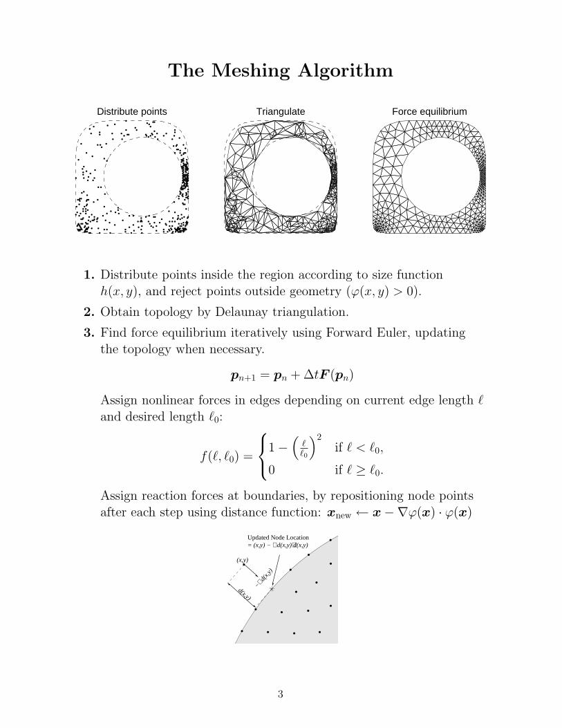
Results (2-D)
2-D Meshes
(1a) (1b) (1c)
(2) (3a) (3b)
(4) (5)(6)
(7)(8)
4
Results (3-D and 4-D)
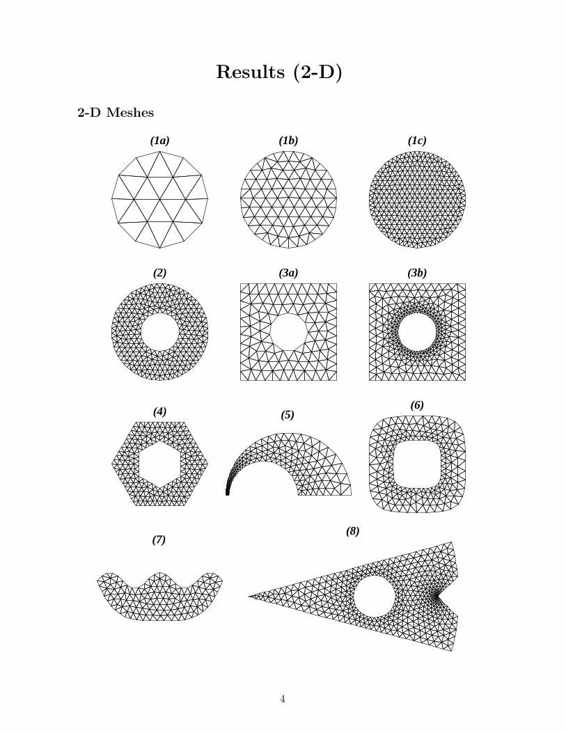
3-D Meshes
• Tetrahedral meshes of unit ball (left) and cylinder with hole (right)
• Surface mesh plots and “split views”
4-D Hypersphere
• ϕ(x) = r − 1 with r =√∑4
i=1 x2i
• h0 = 0.2 gives 3, 458 nodes and 59, 222 elements
• No plots, hard to visualize! Instead indirect verifications:
– Mesh volume V4 = 4.74 (expected value π2/2 ≈ 4.93)
– Hyper-surface area S4 = 16.3 (surface area 2π2 ≈ 19.7 of a 4-Dball). Deviations because of the approximation of the curvedsurface with simplices.
– Poisson’s equation −∇2u = 1, bnd cond’s u = 0|r=1. Analyticalsolution u = (1− r2)/8, linear FEM error ‖e‖∞ = 7.9 · 10−4.
5

Automatic Generation of Size Functions
• Systematic method for computation of h(x) on a background mesh(for example Cartesian grid, but also unstructured meshes)
• Satisfies curvature, feature size, numerical, and grading constraints
• Curvature given by distance function, κ = ∇ · ∇ϕ|∇ϕ|
• PDE-based approach for computation of medial axis transform andlocal feature size
• PDE-based approach for gradient limiting:
h(x) = minx′
(h0(x′) + C‖x− x′‖)
• Numerical adaptive solver easily incorporated
• Generalizes to higher dimensions without modifications
6
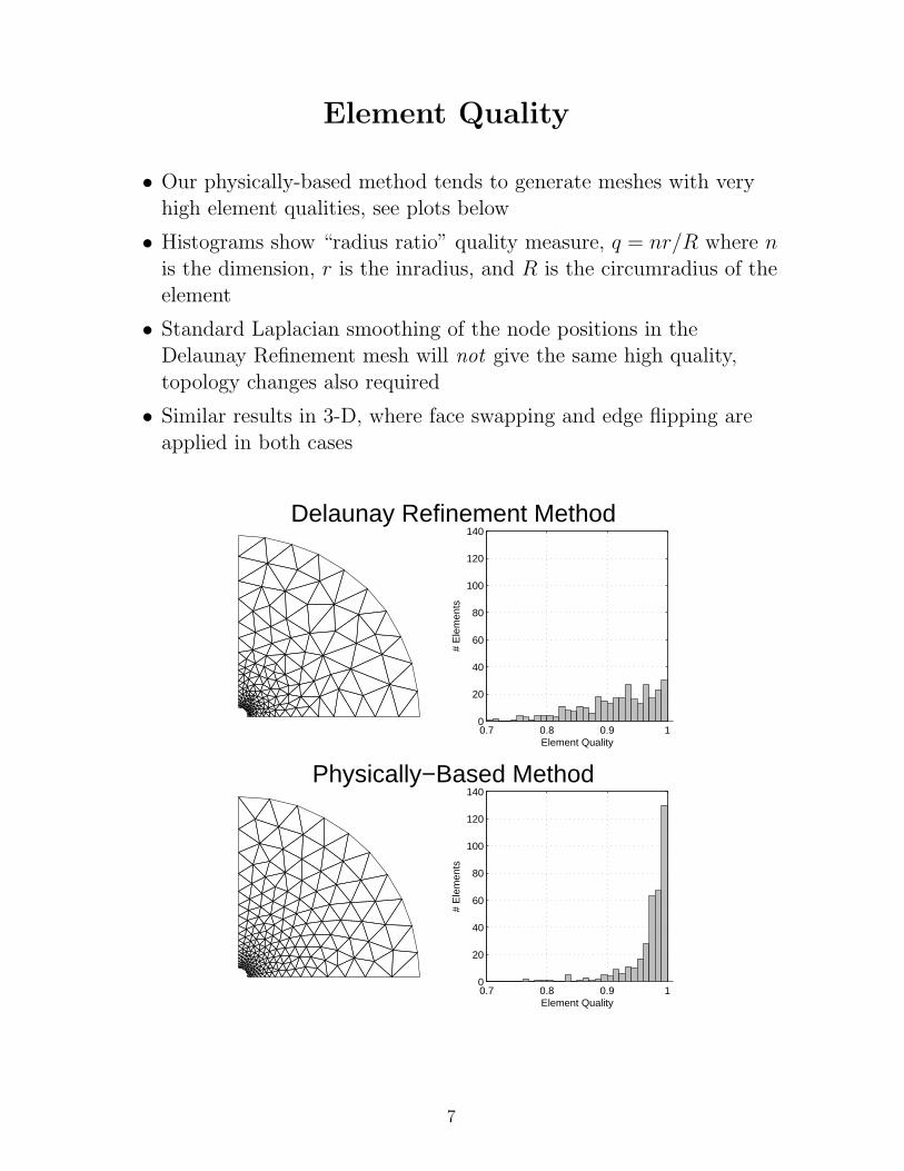
Element Quality
• Our physically-based method tends to generate meshes with veryhigh element qualities, see plots below
• Histograms show “radius ratio” quality measure, q = nr/R where n
is the dimension, r is the inradius, and R is the circumradius of theelement
• Standard Laplacian smoothing of the node positions in theDelaunay Refinement mesh will not give the same high quality,topology changes also required
• Similar results in 3-D, where face swapping and edge flipping areapplied in both cases
0.7 0.8 0.9 10
20
40
60
80
100
120
140
Element Quality
# E
lem
ents
0.7 0.8 0.9 10
20
40
60
80
100
120
140
Element Quality
# E
lem
ents
Delaunay Refinement Method
Physically−Based Method
7

Applications
Numerical Adaptivity
• Model problem: −∆u = 0 in domain, u(r, θ) = sin(4θ/7) onboundary, refinement based on energy norm error estimate
• Interpolate size function h(x) from error indicator on unstructuredmesh from previous iteration
• Use previous mesh as initial condition in iterations, less expensivethan remeshing from scratch
Longest edge refinement Physically based refinement
Moving Interfaces with Topology Changes
• Implicit functions handle topology changes in any dimension
• Use level set method on background mesh for interface propagation
• Multiphase flow, fluid-structure interact., shape optimization, etc
8
Applications
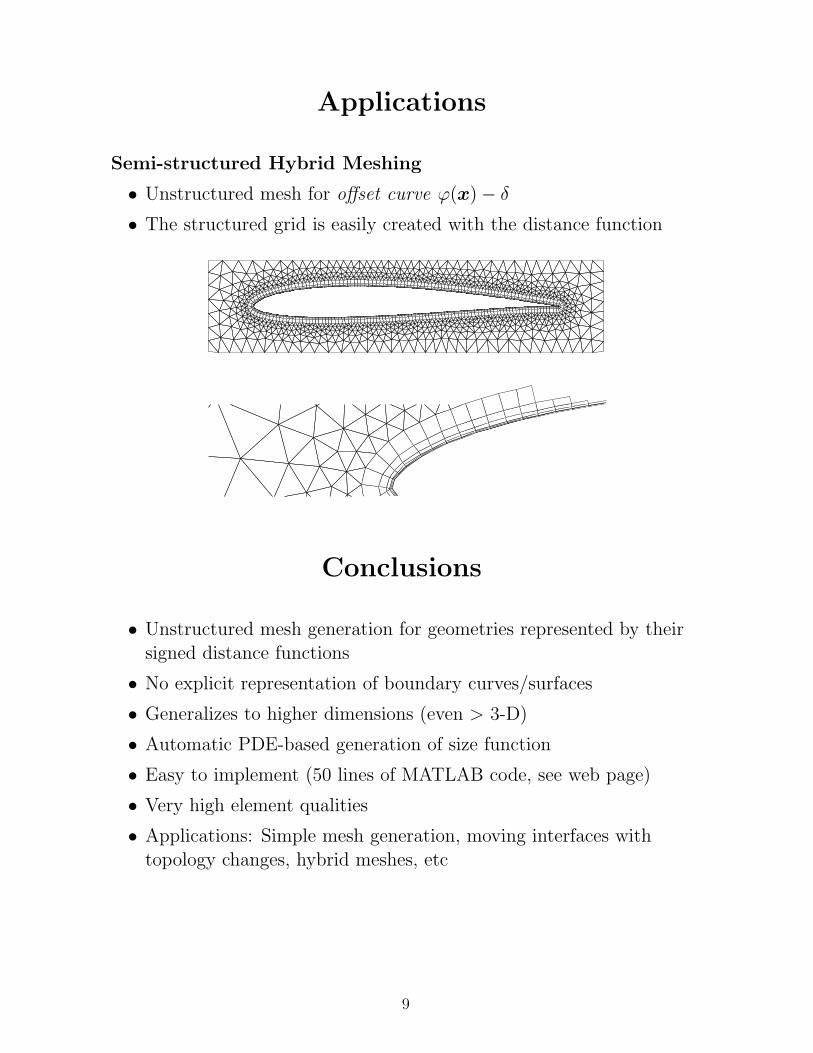
Semi-structured Hybrid Meshing
• Unstructured mesh for offset curve ϕ(x)− δ
• The structured grid is easily created with the distance function
Conclusions
• Unstructured mesh generation for geometries represented by theirsigned distance functions
• No explicit representation of boundary curves/surfaces
• Generalizes to higher dimensions (even > 3-D)
• Automatic PDE-based generation of size function
• Easy to implement (50 lines of MATLAB code, see web page)
• Very high element qualities
• Applications: Simple mesh generation, moving interfaces withtopology changes, hybrid meshes, etc
9