Embed Size (px)
Citation preview

Old Dominion University
University Physics I
Alex Godunov
March 2016


1. Introduction
1
1 Introduction ....................................................................................................................................................................... 1
1.1 The Nature of Physics .......................................................................................................................................... 1
1.2 Physical Quantities and Units ........................................................................................................................... 2
1.3 Unit Prefixes ............................................................................................................................................................. 5
1.4 Unit Consistency and Conversions ................................................................................................................. 6
1.5 Uncertainty and Significant Figures ............................................................................................................... 8
1.6 Estimates and Order of Magnitude ................................................................................................................. 9
1.7 Vectors .................................................................................................................................................................... 10
2 Motion in One Dimension ......................................................................................................................................... 17
2.1 Motion ..................................................................................................................................................................... 17
2.2 Reference Frames, Position and Displacement ...................................................................................... 18
2.3 Velocity and Speed ............................................................................................................................................. 20
2.4 Acceleration .......................................................................................................................................................... 22
2.5 Motion with constant velocity ....................................................................................................................... 24
2.6 Motion with constant acceleration .............................................................................................................. 24
2.7 Freely Falling Bodies ......................................................................................................................................... 28
2.8 Most common problems .................................................................................................................................. 31
2.9 Examples ................................................................................................................................................................ 32
3 Motion in Two Dimensions ...................................................................................................................................... 43
3.1 Position, displacement, velocity and acceleration in 2D and 3D .................................................... 43
3.2 Motion with constant acceleration in 2D .................................................................................................. 45
3.3 Projectile motion................................................................................................................................................. 47
3.4 Motion in a circle................................................................................................................................................. 56
3.5 Relative motion in one and two dimensions ........................................................................................... 58
3.6 Most common problems involving projectile motion ......................................................................... 60
3.7 Examples ................................................................................................................................................................ 61
4 Newton’s Laws of Motion .......................................................................................................................................... 69
4.1 Dynamics ................................................................................................................................................................ 69
4.2 Force and Interaction ........................................................................................................................................ 70

1.1 The Nature of Physics
2
4.3 Newton’s First Law ............................................................................................................................................ 73
4.4 Newton’s Second Law ....................................................................................................................................... 73
4.5 Newton’s Third Law .......................................................................................................................................... 75
4.6 Free body diagrams ........................................................................................................................................... 76
4.7 Examples ................................................................................................................................................................ 77
5 Applying Newton’s Laws ........................................................................................................................................... 81
5.1 Forces ...................................................................................................................................................................... 81
5.2 Dynamics of circular motion .......................................................................................................................... 87
5.3 Few guidelines for solving most common problems in “Applying Newton’s Laws” ............... 88
5.4 Examples ................................................................................................................................................................ 93
6 Kinetic Energy, Work, Power................................................................................................................................. 108
6.1 Energy ................................................................................................................................................................... 108
6.2 Kinetic Energy .................................................................................................................................................... 108
6.3 Scalar (dot) product of vectors ................................................................................................................... 109
6.4 Kinetic energy and work ................................................................................................................................ 110
6.5 Power ..................................................................................................................................................................... 112
6.6 Examples .............................................................................................................................................................. 113
7 Conservation of Energy ............................................................................................................................................ 118
7.1 Potential energy and conservative forces .............................................................................................. 118
7.2 Gravitational and elastic potential energies .......................................................................................... 121
7.3 Non-conservative forces ................................................................................................................................ 122
7.4 Potential energy diagrams ............................................................................................................................ 124
7.5 Guidelines for solving most common problems in “Conservation of energy” ......................... 126
7.6 Examples .............................................................................................................................................................. 127
8 Systems of particles ................................................................................................................................................... 138
8.1 Momentum .......................................................................................................................................................... 139
8.2 The linear momentum of a system of particles .................................................................................... 140
8.3 Newton’s second law for a system of particles..................................................................................... 142
8.4 Impulse and Linear Momentum ................................................................................................................. 144
1. Introduction
3
8.5 Collisions .............................................................................................................................................................. 144
8.6 The center of mass of solid bodies* .......................................................................................................... 149
8.7 Dynamics of Bodies of Variable Mass; Rocket propulsion ............................................................... 150
8.8 Examples .............................................................................................................................................................. 151
9 Rotation in two dimensions ................................................................................................................................... 162
9.1 Rotational motion ............................................................................................................................................. 162
9.2 Rotational variables ......................................................................................................................................... 163
9.3 Rotation with constant angular acceleration ........................................................................................ 166
9.4 Relating the linear and angular variables ............................................................................................... 167
9.5 Kinetic energy of rotation ............................................................................................................................. 169
9.6 Calculating the rotational inertia ............................................................................................................... 170
9.7 Potential energy of a rigid body.................................................................................................................. 172
9.8 Examples .............................................................................................................................................................. 173
10 Dynamics of rotational motion ........................................................................................................................ 178
10.1 Torque ................................................................................................................................................................... 178
10.2 Vector Product ................................................................................................................................................... 179
10.3 Torque as a vector product ........................................................................................................................... 180
10.4 Newton’s Second Law for rotation ............................................................................................................ 180
10.5 Rolling.................................................................................................................................................................... 182
10.6 Translation and rotation dynamics ........................................................................................................... 186
10.7 Work and Power in Rotational Motion .................................................................................................... 186
10.8 Angular momentum ......................................................................................................................................... 187
10.9 Examples .............................................................................................................................................................. 190
11 Equilibrium .............................................................................................................................................................. 203
11.1 The conditions for equilibrium ................................................................................................................... 203
11.2 The center of gravity ....................................................................................................................................... 206
11.3 Few more words ............................................................................................................................................... 207
11.4 Statically undetermined systems ............................................................................................................... 208
11.5 Few guidelines for solving most common problems in “Equilibrium” ....................................... 209

1.1 The Nature of Physics
4
11.6 Examples .............................................................................................................................................................. 211
12 The Law of Gravitation ........................................................................................................................................ 231
12.1 Newton’s law of gravitation ......................................................................................................................... 231
12.2 Acceleration due to gravity g ....................................................................................................................... 236
12.3 Gravitational potential energy .................................................................................................................... 238
12.4 Motion of planets and satellites .................................................................................................................. 239
12.5 Planets and satellites: circular orbits, escape speed. ......................................................................... 241
12.6 Examples .............................................................................................................................................................. 244
13 Periodic Motion ...................................................................................................................................................... 245
13.1 Simple harmonic motion ............................................................................................................................... 245
13.2 Energy of the simple harmonic motion ................................................................................................... 249
13.3 Applications of simple harmonic motion ................................................................................................ 250
13.4 Simple harmonic motion and circular motion ...................................................................................... 253
13.5 Damped and forced oscillations* ............................................................................................................... 254
13.6 Examples .............................................................................................................................................................. 256
14 Fluids .......................................................................................................................................................................... 260
14.1 Density and pressure ...................................................................................................................................... 260
14.2 Hydrostatics ........................................................................................................................................................ 261
14.3 Hydrodynamics ................................................................................................................................................. 268
14.4 Examples .............................................................................................................................................................. 272
15 Waves ......................................................................................................................................................................... 274
15.1 Mechanical waves (physics behind the scene) ..................................................................................... 274
15.2 Wave equation* ................................................................................................................................................. 276
15.3 Sinusoidal waves ............................................................................................................................................... 278
15.4 Power transferred by a wave ....................................................................................................................... 280
15.5 Interference and reflection of waves ........................................................................................................ 281
15.6 Sound waves ....................................................................................................................................................... 282

1. Introduction
1
1 Introduction
“All science is either physics or stamp collecting.”
Ernest Rutherford
1.1 The Nature of Physics
Physics is the most fundamental and all-inclusive of the sciences, and has had a profound effect on all
scientific development. Scientists of all disciplines make use of ideas, laws, methods and techniques
of physics. Physics is the foundation of all science, engineering and technology. Students of many
fields find themselves studying physics because of the basic role it plays in all phenomena.
Richard Feynman has a beautiful description of the nature of physics in “The Feynman Lectures on
Physics.” The book can be found at http://www.feynmanlectures.caltech.edu/I_toc.html
The next few paragraphs in this section are based on his book.
If you are going to learn physics, you will have a lot to study: two hundred years of the most rapidly
developing field of knowledge that there is. Surprisingly enough, in spite of the tremendous amount
of work that has been done for all this time it is possible to condense the enormous mass of results to
a large extent—that is, to find laws which summarize all our knowledge. Even so, the laws are so hard
to grasp that it is unfair to you to start exploring this tremendous subject without some kind of map
or outline of the relationship of one part of the subject of science to another.
You might ask why we cannot teach physics by just giving the basic laws on page one and then
showing how they work in all possible circumstances. We cannot do it in this way for two reasons.
First, we do not yet know all the basic laws: there is an expanding frontier of ignorance. Second, the
correct statement of the laws of physics involves some very unfamiliar ideas which require advanced

1.2 Physical Quantities and Units
2
mathematics for their description. Therefore, one needs a considerable amount of preparatory
training even to learn what the words mean. No, it is not possible to do it that way. We can only do it
piece by piece.
Each piece, or part, of the whole of nature is always merely an approximation to the complete truth,
or the complete truth so far as we know it. In fact, everything we know is only some kind of
approximation, because we know that we do not know all the laws as yet. Therefore, things must be
learned only to be unlearned again or, more likely, to be corrected.
The principle of science, the definition, almost, is the following: The test of all knowledge is
experiment. Experiment is the sole judge of scientific "truth." But what is the source of knowledge?
Where do the laws that are to be tested come from? Experiment, itself, helps to produce these laws,
in the sense that it gives us hints. But also needed is imagination to create from these hints the great
generalizations - to guess at the wonderful, simple, but very strange patterns beneath them all, and
then to experiment to check again whether we have made the right guess. This imagining process is
so difficult that there is a division of labor in physics: there are theoretical physicists who imagine,
deduce, and guess at new laws, but do not experiment; and then there are experimental physicists
who experiment, imagine, deduce, and guess.
Now, what should we teach first? Should we teach the correct but unfamiliar law with its strange and
difficult conceptual ideas, for example the theory of relativity, four-dimensional space-time, and so
on? Or should we first teach the simple "constant-mass" law, which is only approximate, but does not
involve such difficult ideas? The first is more exciting, more wonderful, and more fun, but the second
is easier to get at first, and is a first step to a real understanding of the second idea. This point arises
again and again in teaching physics. At different times we shall have to resolve it in different ways,
but at each stage it is worth learning what is now known, how accurate it is, how it fits into everything
else, and how it may be changed when we learn more.
1.2 Physical Quantities and Units
Physics is an experimental science, based on measurements. Theory plays a major role in
understanding. We measure each physical quantity in its own units, by comparison with a standard.
The standard corresponds to 1.0 unit of the quantity.
Scientists measure all sorts of things in their observations and experiments. Many quantities can be
determined by measuring others and then combining the measurements according to the laws of
physics.
There are very many physical quantities, but practically all physical processes, characteristics and
phenomena can be expressed in terms of a small number of independent, fundamental quantities.
There are seven fundamental (or base) quantities forming the basis of the International System of
Units, commonly known as SI units, from the French Système International d'Unités.

1. Introduction
3
Table 1.1 Fundamental quantities and their SI units
Quantity Units Abbreviation
length meter m
time second s
mass kilogram kg
temperature kelvin K
electric current ampere A
amount of substance mole mol
light intensity candela cd
Although, the choice of the units is arbitrary (they have been defined by humans rather than
prescribed by nature), the SI units is the most widely used system in the word.
For the first semester of university physics we mostly need three base units: length, time, and mass.
1.2.1 Length
In the late 1700s the French Academy of Sciences declared the meter to be a specific fraction
(1/10,000,000) of the distance from Earth’s equator to the North Pole (at sea level).
In the 1870s and in light of modern precision, a series of international conferences was held to devise
new metric standards. In 1889 at the first General Conference on Weights and Measures the
International Prototype Metre was established as the distance between two lines on a standard bar
composed of an alloy of ninety percent platinum and ten percent iridium, measured at the melting
point of ice. That bar was a standard from 1889 to 1960.
Today the meter is defined by the distance light travels in a vacuum in 1/299,792,458 of a second.
Thus, the meter is based on postulated speed of light.
Historical context of the meter can be found at http://physics.nist.gov/cuu/Units/meter.html
1.2.2 Time
Between middle ages and 1960 the second was defined as 1/86,400 of a mean solar day. The exact
definition of "mean solar day" was left to astronomical theories. However, measurement showed that
irregularities in the rotation of the Earth could not be taken into account by the theory and has the
effect that this definition does not allow the required accuracy to be achieved.
Now the second is defined as the time it takes for 9,192,631,770 periods of the transition between
two split levels of the ground state of the cesium-133 atom.
By the way, in science we still have troubles to have a good definition of time. Webster defines "a
time" as "a period," and the latter as "a time," which doesn't seem to be very useful. Here are a couple

1.2 Physical Quantities and Units
4
quotes from great scientists: “The only reason for time is so that everything doesn't happen at once”
Albert Einstein, "Time is what happens when nothing else happens" Richard Feynman.
1.2.3 Mass
At the end of the 18th century, a kilogram was the mass of a cubic decimeter (1 liter) of water. In
1889, the 1st The General Conference on Weights and Measures (Conférence Générale des Poidset
Mesures, CGPM) sanctioned the international prototype of the kilogram, made of platinum-iridium,
and declared: This prototype shall henceforth be considered to be the unit of mass.
The 3d CGPM (1901), in a declaration intended to end the ambiguity in popular usage concerning the
word "weight," confirmed that: The kilogram is the unit of mass; it is equal to the mass of the
international prototype of the kilogram.
1.2.4 How large?
Many physicists find it helpful to have an intuitive feel for the sizes of magnitudes. This is especially
true if you grew up using the English system of units.
Table 1.2 For orientation
Quantity Units Good to know
mass kilogram The mass of a 1-L bottle of water
distance meter An average height of a man in the US is 1.8 m
distance kilometer If you are an average person you can walk 1 km in
about 12 minutes
speed meter/second An average person walk with a speed of 1.4 m/s
energy joule An apple that falls from a table has about 1 J of
kinetic energy
power watt An average laptop uses from 50 to 70 W
1.2.5 Derived units
Most other units are derived or based on fundamental (base) units. Examples of derived units: area
(m2), speed (m/s), and mass density (kg/m3).
We use variables to represent the values of physical quantities and relationships between them. For
many quantities we use standard notations (letter, symbols), like 𝑚 for mass, 𝑣 for velocity, 𝑡 for time,
𝑝 for momentum, 𝐸 for energy, 𝜔 for angular speed, etc.
1.2.6 The British system of units
These units (also called British Imperial system of units) are used only in the United States and remain
in limited use in India, Malaysia, Sri Lanka, Hong Kong, and some Caribbean islands. British units are
now officially defined in terms of SI units as follow Length: 1 inch = 2.54 cm (exactly),

1. Introduction
5
Force: 1 pound = 4.448221615260 newtons (exactly). The British unit of time is the second, defined
the same way as in SI. There is no British system of electrical units. The British system has very
complicated relations between base and derived units.
Table 1.3 Linear measures in the British system of units
Unit 1 Unit 2
12 inches (in) 1 foot (ft)
3 feet 1 yard (yd)
5 1/2 yards 1 rod (rd)
40 rods 1 furlong (fur) = 220 yards = 660 ft
8 furlongs 1 statute mile (mi) = 1,760 yards
5,280 feet 1 statute or land mile
From lectures of Professor Lewin (Massachusetts Institute of Technology) “I find it extremely difficult
to work with inches and feet. It's an extremely uncivilized system. I don't mean to insult you, but think
about it - 12 inches in a foot, three feet in a yard. Could drive you nuts”.
Going a bit beyond nuisance of the British system of units - think about it. What is the first day of a
week? If it is Sunday why do we call it weekend!
Note: you should try to think in SI units as much as you can!
1.3 Unit Prefixes
In physics, we explore the very small to the very large. The very small is a small fraction of a proton
and the very large is the universe itself. For example, the horizontal size of the Universe is about
2.6*1026 m, the size of an electron is about 5.6*10-15 m. They span 45 orders of magnitude. In scientific
notations: 1000,000,000,000,000,000,000,000,000,000,000,000,000,000,000 = 1.0*1045. Once we
have defined the fundamental units, it is easy to introduce large and smaller units for the same
physical quantities. In the metric system these other units are related to the fundamental units by
multipliers of 10 or 1/10.
Table 1.4 Prefixes
Factor Prefix Symbol Factor Prefix Symbol Factor Prefix Symbol
𝟏𝟎−𝟐𝟒 yocto y 10−3 milli m 109 giga G
𝟏𝟎−𝟐𝟏 zepto z 10−2 centi c 1012 tera T
𝟏𝟎−𝟏𝟖 attpo a 10−1 deci d 1015 peta P
𝟏𝟎−𝟏𝟓 femto a 101 deka da 1018 exa E
𝟏𝟎−𝟏𝟐 pico p 102 hecto h 1021 zetta Z
𝟏𝟎−𝟗 nano n 103 kilo k 1024 yotta Y
𝟏𝟎−𝟔 micro 𝜇 106 mega M 10100 googol

1.4 Unit Consistency and Conversions
6
Thus, 1 kilometer (1 km) is 1000 meters (1 km = 103 m), 1 centimeter (1 cm) is 1/100 meter (1 cm =
10-2 m).
The names of additional units are derived by adding a prefix to the name of the fundamental unit.
Attention: Don’t drop the prefixes. For example 700 nm is less than 0.7 m.
Prefixes are a convenient way to express large and small numbers, but use them with care. You are
guaranteed consistency when all of the numbers you are entered into a calculation are in the SI units.
For example, in calculations use meters not kilometers.
1.4 Unit Consistency and Conversions
We use equations to express relationships among physical quantities, represented by algebraic
symbols. Each symbol always represents both a number and a unit.
1.4.1 Dimensional Analysis
An equation must be dimensionally consistent. Dimensional analysis is a powerful technique that can
help you quickly determine how likely it is that you have done a problem correctly. You check that
the dimensions of you algebraic answer matches what you expect before you substitute values to
computer a numerical result.
Any mechanical quantity can be represented as[𝐴] = 𝑀𝑥𝐿𝑦𝑇𝑧.
Table 1.5 Dimensions of Some Mechanical Quantities
Quantity Dimension Units
length 𝐿 𝑚
time 𝑇 s
mass 𝑀 𝑘𝑔
velocity 𝐿 ∙ 𝑇−1 𝑚 ∙ 𝑠−1
acceleration 𝐿 ∙ 𝑇−2 𝑚 ∙ 𝑠−2
volume 𝐿3 𝑚3
density 𝑀 ∙ 𝐿−3 𝑘𝑔 ∙ 𝑚−3
force 𝑀 ∙ 𝐿 ∙ 𝑇−2 𝑘𝑔 ∙ 𝑚 ∙ 𝑠−2 =newton
energy 𝑀 ∙ 𝐿2 ∙ 𝑇−2 𝑘𝑔 ∙ 𝑚2 ∙ 𝑠−2 =joule
Example 1: The period of a simple pendulum, the time for one complete oscillation, is given by 𝑇 =
2𝜋√𝐿/𝑔, where L is the length of the pendulum and 𝑔 is the acceleration due to gravity. Show that the
dimension is consistent.
𝑇 = √𝐿
(𝐿 ∙ 𝑇−2)= √𝑇2 = 𝑇

1. Introduction
7
Example 2: A proof of Pythagorean Theorem using dimensional analysis. The area 𝐴 of the right-angle
triangle is a function of the angle and the hypotenuse (for a right-angled triangle, only the hypotenuse
length and one of the angles are needed to completely specify the triangle), or 𝐴𝑐 = 𝑓(𝑐, 𝛼). Since
area’s dimension is [𝐴𝑟𝑒𝑎] = 𝐿2, then 𝑓(𝑐, 𝛼) = 𝑐2𝑔(𝛼), where 𝑔(𝛼) is a dimensionless function of the
angle.
For smaller triangles inside the original one we can write 𝐴𝑎 = 𝑎2𝑔(𝛼) and 𝐴𝑏 = 𝑏2𝑔(𝛼). It is obvious
that 𝐴𝑐 = 𝐴𝑎 + 𝐴𝑏 or 𝑐2𝑔(𝛼) = 𝑎2𝑔(𝛼) + 𝑏2𝑔(𝛼), then 𝑐2 = 𝑎2 + 𝑏2.
1.4.2 Unit Conversion
We often need to change the units in which a physical quantity is expressed. We do so by a method
called chain-link conversion. In this method we multiple the original value by a conversion factor (a
ratio of units that is equal to unity). For example, 1 min = 60 s, then (1 min/60 s) =1 as well as
(60 s/1 min) =1.
Example: Let’s find number of minutes in 150 seconds:
correct: 150 𝑠 = 150 𝑠 ∙ 1 = 150 𝑠 (1 𝑚𝑖𝑛
60 𝑠) = 2.5 𝑚𝑖𝑛
incorrect: 150 𝑠 = 150 𝑠 ∙ 1 = 150 𝑠 (60 𝑠
1 𝑚𝑖𝑛) = 9000 𝑚𝑖𝑛 because you get 9000 𝑠2/𝑚𝑖𝑛
Attention 1: to ensure that you have written the conversion factor properly, check that the units
cancel as necessary between numerator and denominator.
Attention 2: Some conversion cannot be easily carried out in a single step. Then, write each phase of
a conversion separately.
Example 1: There is no speed limit on the German autobahn, but recommended top speed is
130 km/h. Let’s express this speed in miles per hour and meters per second,
where 1 mile = 1.609 km = 1609 m, 1 km = 1000 m, 1 h = 3600 s.
130 𝑘𝑚 ℎ⁄ = (130 𝑘𝑚
1 ℎ) (
1 𝑚𝑖𝑙𝑒
1.609 𝑘𝑚) = 80.8 𝑚𝑝ℎ
130 𝑘𝑚 ℎ =⁄ (130 𝑘𝑚
1 ℎ) (
1000 𝑚
1 𝑘𝑚) (
1 ℎ
3600 𝑠) = 36.1 𝑚 𝑠⁄
Example 2: How many square centimeters in a square meter? (Note that 1 m = 100 cm)
1 𝑚2 = (1 𝑚)2 = [1 𝑚 (100 𝑐𝑚
1 𝑚)]
2
= [100 𝑐𝑚]2 = 10,000 𝑐𝑚2

1.5 Uncertainty and Significant Figures
8
1.5 Uncertainty and Significant Figures
Measurements always have uncertainties. The uncertainty is also called the error because it indicates
the maximum difference there is likely to be between the measured value and the true value. We often
indicate the accuracy of a measured value with the symbol ±, i.e. is a length of a pencil is given as 56.47
± 0.02 mm, this means that the true value is unlikely to be less than 56.45 mm or greater than
56.49 mm.
There are statistical methods for determining the error in a calculation that are beyond the scope of
this course. We will use a simplified approach called “significant figures.”
For example, a distance is given as 137 km. It has three significant figures. By this we mean that the
first two digits are known to be correct, while the third digit is uncertain, and the uncertainty is about
1 km.
Example: How many miles in 2000 meters? (1 mile = 1609 m)? In this example, when we say that the
distance is 2000 meters, we mean, first, that it is neither 1999 meters nor 2001 meters, and, second,
that we do not bother if the distance is more precisely, say, 1999 meters and 70 centimeters: we round
it up to 2000 meters. In other words, 2000 meters in this context means some number between
1999.5 and 2000.5
Calculations give
2000.5
1609= 1.243318831572405 and
1999.5
1609= 1.242697327532629
Comparing these numbers, we conclude that we should write 2000 𝑚 (1 𝑚𝑖𝑙𝑒
1609 𝑚) = 1.243 𝑚𝑖𝑙𝑒
discarding further insignificant figures.
1.5.1 Significant figures in multiplication or division
Suppose that we measured one side of a rectangle and obtained that it equals 5.77 cm. The other side,
for some reason, we measured with a cruder ruler and obtained that its length is 9.9 cm. If, to find the
area, we simply multiply these numbers, the calculator gives (5.77 cm)*(9.9 cm) = 57.123 cm2.
However, realizing that we deal with rounded numbers, to check what are possible outcomes, we
multiply the lower admissible values (5.765 cm)*(9.85 cm) = 56.78525 cm2 and also the higher
admissible values (5.775 cm)*(9.95 cm) = 57.46125 cm2. Thus, we have a rather wide range of values
for the area. Keeping more than two figures clearly makes no sense. So, discarding insignificant
figures and rounding to two figures, we obtain (5.77 cm)*(9.9 cm) = 57 cm2, where “57” is the properly
rounded version of the original “57.123”. For further uses, “57” should be understood as a number
between 56.5 and 57.5.
A simple inspection shows that uncertainty in the value of the product is determined mainly by the
uncertainty in the value 9.9 cm of the least precise measurement.
Rule of thumb: do not keep more figures than in the least precise input term.
1. Introduction
9
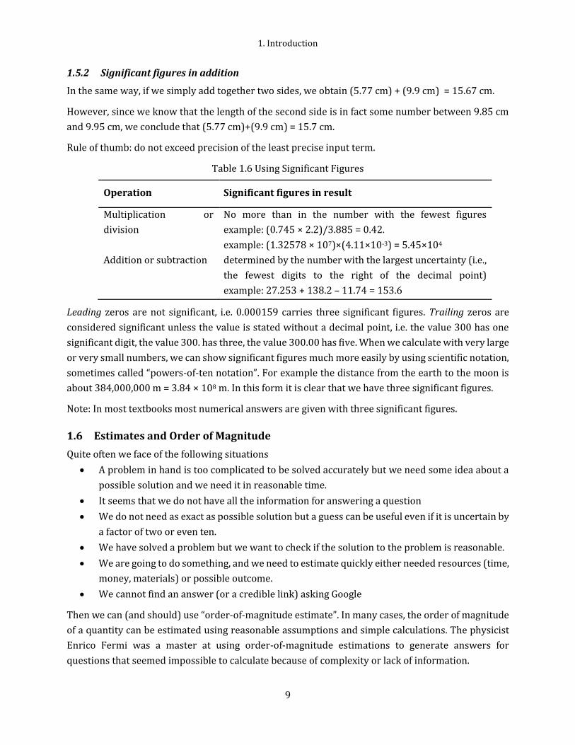
1.5.2 Significant figures in addition
In the same way, if we simply add together two sides, we obtain (5.77 cm) + (9.9 cm) = 15.67 cm.
However, since we know that the length of the second side is in fact some number between 9.85 cm
and 9.95 cm, we conclude that (5.77 cm)+(9.9 cm) = 15.7 cm.
Rule of thumb: do not exceed precision of the least precise input term.
Table 1.6 Using Significant Figures
Operation Significant figures in result
Multiplication or
division
No more than in the number with the fewest figures
example: (0.745 × 2.2)/3.885 = 0.42.
example: (1.32578 × 107)×(4.11×10-3) = 5.45×10⁴
Addition or subtraction determined by the number with the largest uncertainty (i.e.,
the fewest digits to the right of the decimal point)
example: 27.253 + 138.2 – 11.74 = 153.6
Leading zeros are not significant, i.e. 0.000159 carries three significant figures. Trailing zeros are
considered significant unless the value is stated without a decimal point, i.e. the value 300 has one
significant digit, the value 300. has three, the value 300.00 has five. When we calculate with very large
or very small numbers, we can show significant figures much more easily by using scientific notation,
sometimes called “powers-of-ten notation”. For example the distance from the earth to the moon is
about 384,000,000 m = 3.84 × 10⁸ m. In this form it is clear that we have three significant figures.
Note: In most textbooks most numerical answers are given with three significant figures.
1.6 Estimates and Order of Magnitude
Quite often we face of the following situations
A problem in hand is too complicated to be solved accurately but we need some idea about a
possible solution and we need it in reasonable time.
It seems that we do not have all the information for answering a question
We do not need as exact as possible solution but a guess can be useful even if it is uncertain by
a factor of two or even ten.
We have solved a problem but we want to check if the solution to the problem is reasonable.
We are going to do something, and we need to estimate quickly either needed resources (time,
money, materials) or possible outcome.
We cannot find an answer (or a credible link) asking Google
Then we can (and should) use “order-of-magnitude estimate”. In many cases, the order of magnitude
of a quantity can be estimated using reasonable assumptions and simple calculations. The physicist
Enrico Fermi was a master at using order-of-magnitude estimations to generate answers for
questions that seemed impossible to calculate because of complexity or lack of information.

1.7 Vectors
10
Using order-of-magnitude estimations is not restricted to science but is commonly used in
engineering, business, medicine, practically anywhere. When you master the order-of-magnitude
estimations then you can see that very many episodes in movies from Hollywood are far from reality.
For using the order-of-magnitude estimations we need to
1. come up with as simple as possible model for our problem or question (“Make things as simple
as possible, but not simpler” - Albert Einstein). Breaking dawn a problem into easier smaller
problems may work as well.
2. figure out what data do we need for our model
3. get the required data using present knowledge, common sense, educated guess (by bracketing
missing data and applying either geometric mean) or asking Google if possible
4. carry out (normally very simple) calculations
If we feel that our order-of-magnitude estimation is sensible we can stop here. There are a couple
principal reasons when we fail, namely, oversimplified or wrong model and wrong estimation for
data.
Here are a couple of such questions that can be answered using reasonable assumptions.
How much money one needs to drive from Norfolk, VA to Los Angeles, CA?
How much coffee is consumed daily by ODU students?
What is the radius the radius of Earth?
For mastering the art of estimation one may read
”Guesstimation 2.0: Solving Today’s Problems on the Back of a Napkin”
by Lawrence Weinstein, Princeton University Press (2012)
“How Many Licks?: Or, How to Estimate Damn Near Anything”
by Aaron Santos, Running Press (2009)
One may find interesting to read “How to Measure Anything: Finding the Value of Intangibles in
Business” by Douglas W. Hubbard, 3rd edition, Wiley (2014)
1.7 Vectors
1.7.1 Coordinate systems
Very many quantities in physics deal with locations in space, for example, a position of an object at
different moments in time. We need to define a coordinate system to describe the position of a point
in space relative to some origin. There are multiple types of coordinate systems. The most popular
systems in physics are Cartesian, polar, cylindrical, and spherical coordinate systems.
1. Introduction
11
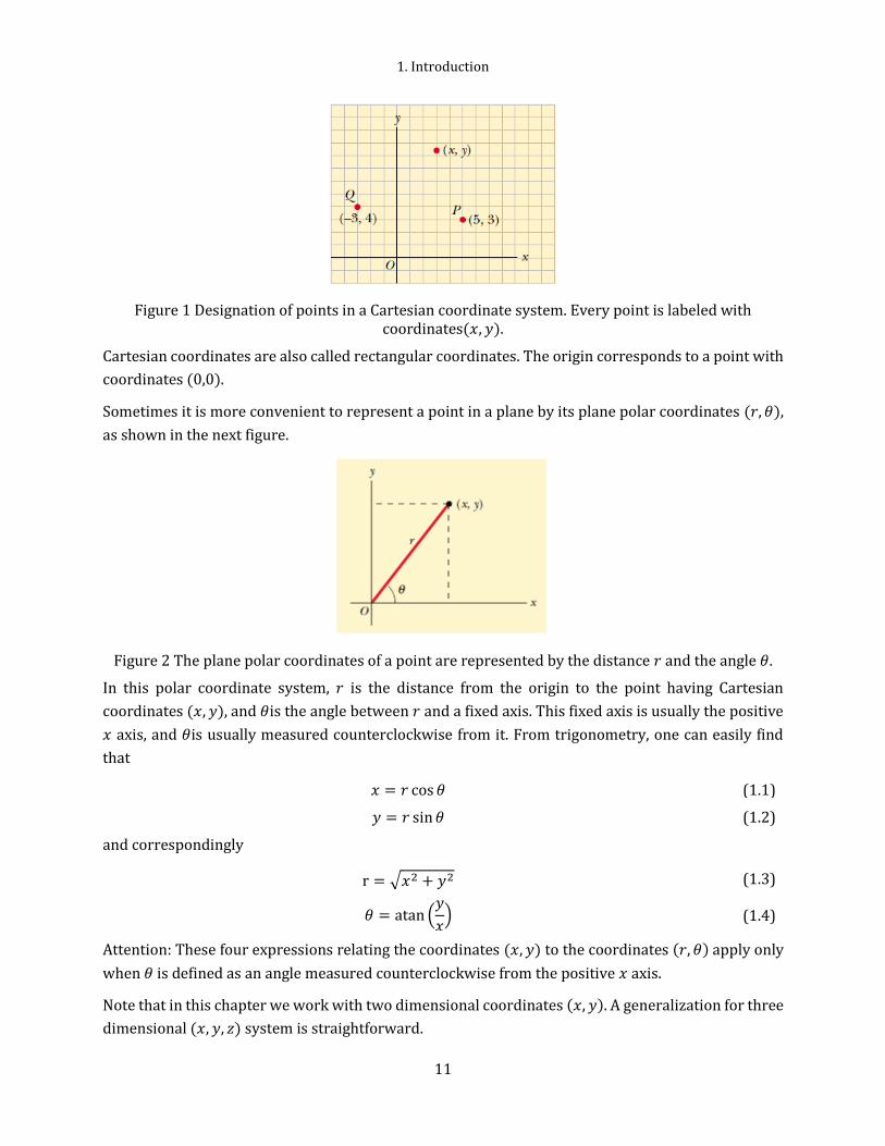
Figure 1 Designation of points in a Cartesian coordinate system. Every point is labeled with coordinates(𝑥, 𝑦).
Cartesian coordinates are also called rectangular coordinates. The origin corresponds to a point with
coordinates (0,0).
Sometimes it is more convenient to represent a point in a plane by its plane polar coordinates (𝑟, 𝜃),
as shown in the next figure.
Figure 2 The plane polar coordinates of a point are represented by the distance 𝑟 and the angle 𝜃.
In this polar coordinate system, 𝑟 is the distance from the origin to the point having Cartesian
coordinates (𝑥, 𝑦), and 𝜃is the angle between 𝑟 and a fixed axis. This fixed axis is usually the positive
𝑥 axis, and 𝜃is usually measured counterclockwise from it. From trigonometry, one can easily find
that
𝑥 = 𝑟 cos 𝜃 (1.1)
𝑦 = 𝑟 sin 𝜃 (1.2)
and correspondingly
r = √𝑥2 + 𝑦2 (1.3)
𝜃 = atan (𝑦
𝑥) (1.4)
Attention: These four expressions relating the coordinates (𝑥, 𝑦) to the coordinates (𝑟, 𝜃) apply only
when 𝜃 is defined as an angle measured counterclockwise from the positive 𝑥 axis.
Note that in this chapter we work with two dimensional coordinates (𝑥, 𝑦). A generalization for three
dimensional (𝑥, 𝑦, 𝑧) system is straightforward.

1.7 Vectors
12
1.7.2 Scalars and vectors
In our daily lives we deal, as a rule, with quantities that are completely specified by its magnitude, a
single number, together with the units in which it is measured. Such a quantity is called a scalar and
examples include temperature, time, and density.
However, there are very many physical quantities that require both a magnitude (≥ 0) and a direction
in space to specify them completely. They are caller vectors. A familiar example is force, which has a
magnitude (strength) and a direction of application. Vectors are also used to describe physical
quantities such as velocity, displacement, momentum, electric field, and many more. A vector is
usually indicated by either an arrow over a letter representing a physical quantity (e.g. �⃗�) or by a
boldface letter (e.g. 𝒂). A vector can be conveniently represented as an arrow in space.
Figure 3 Three vectors in 𝑥, 𝑦 plane
The length of the arrow representing a vector �⃗� is called the length or the magnitude of 𝑎 (written as
|𝑎| or just 𝑎 where 𝑎 ≥ 0). Note the use of 𝑎 to means the magnitude of �⃗�; for this reason it is important
to make it clear whether you mean a vector or its magnitude (which is a scalar). The magnitude
together with the angles provides a complete description of a vector. For example, in a two-
dimensional case a set of the two numbers 𝑎 and 𝜃 uniquely describe vector �⃗�.
Figure 4 A vector in 𝑥𝑦 plane.
The same vector can also be uniquely described with the components of the vector 𝑎𝑥 , 𝑎𝑦 where
𝑎𝑥 = 𝑎 cos 𝜃 (1.5)
𝑎𝑦 = 𝑎 sin 𝜃 (1.6)
1.7.3 Addition and subtraction of vectors
So far we only need to learn how to add two (or more vectors) and to multiple a vector by a scalar.
Vector products (dot and cross) will be introduced later.

1. Introduction
13
Two vectors �⃗�and �⃗⃗� are defined to be equal if they have the same magnitude and point in the same
direction. That is, �⃗� = �⃗⃗� only if 𝑎 = 𝑏 and if �⃗� and �⃗⃗� point in the same direction along parallel lines.
Figure 5 These two vectors are equal because they have equal lengths and point in the same direction.
For example, two vectors in Figure 5 are equal even though they have different starting points. This
property allows us to move a vector to a position parallel to itself in a diagram without affecting the
vector.
The rules for adding vectors are conveniently described by geometric methods. To add vector �⃗⃗� to
vector �⃗�, first draw vector �⃗�, with its magnitude represented by a convenient scale, on graph paper
and then draw vector �⃗⃗� to the same scale with its tail starting from the tip of �⃗�, as shown in Figure 6.
The resultant vector 𝑐 = �⃗� + �⃗⃗� is the vector drawn from the tail of �⃗� to the tip of �⃗⃗�.
Figure 6 A vector sum 𝑐 = �⃗� + �⃗⃗� (the triangle method of addition).
When two vectors are added, the sum is independent of the order of the addition. (This fact may seem
trivial, but as you will later, the order is important when vectors are multiplied). This can be seen
from the geometric construction above and is known as the commutative law of addition:
𝑐 = �⃗� + �⃗⃗� = �⃗⃗� + �⃗�. (1.7)
An alternative graphical procedure for adding two vectors is called the parallelogram rule of addition.
In this construction, the tails of the two vectors �⃗� and �⃗⃗� are joined together and the resultant vector 𝑐
isthe diagonal of a parallelogram formed with �⃗� and �⃗⃗� as two of its four sides.
Figure 7 A vector sum 𝑐 = �⃗� + �⃗⃗� (the parallelogram method of addition).

1.7 Vectors
14
The negative of the vector �⃗� is defined as the vector that when added to �⃗� gives zero for the vector
sum, that is �⃗� + (−�⃗�) = 0. The vectors �⃗� and −�⃗� have the same magnitude but point in opposite
directions.
The operation of vector subtraction makes use of the definition of the negative of a vector. We define
the operation �⃗� − �⃗⃗� as vector −�⃗⃗� added to vector �⃗�:
�⃗� − �⃗⃗� = �⃗� + (−�⃗⃗�). (1.8)
If vector �⃗� is multiplied by a positive scalar quantity 𝑛, then the product 𝑛�⃗� is a vector that has the
same direction as �⃗� and magnitude 𝑛𝑎. If vector �⃗� is multiplied by a negative scalar quantity −𝑛, then
the product −𝑛�⃗� is directed opposite �⃗�.
1.7.4 Multiplication by a scalar
Multiplication of a vector by a scalar (not to be confused with the ‘scalar product’, to be discussed in
section 6.3) gives a vector in the same direction as the original but of a proportional magnitude. This
can be seen in figure.
The scalar may be positive, negative or zero. (It can also be complex in some applications). Clearly,
when the scalar is negative we obtain a vector pointing in the opposite direction to the original vector.
Having defined the operations of addition, subtraction and multiplication by a scalar, we can now
introduce unit vectors and components.
1.7.5 Unit vectors and components of a vector
While geometric methods for adding or subtracting vectors are rather simple, they are not practical
for solving problems. Using vector components is a much more accurate way with less room for
making a mistake.
Figure 8 Two unit vectors 𝑖̂ and 𝑗̂.
A unit vector is a vector that has a magnitude of exactly 1 and points in a particularly direction. It
lacks both dimensions and unit. Its sole purpose is to point – that is, to specify a direction. The unit
vectors in the positive directions of the 𝑥, 𝑦 and 𝑧 axes are labeled as 𝑖̂, 𝑗̂ and �̂�.

1. Introduction
15
Consider a vector �⃗� lying in the 𝑥𝑦 plane and making an arbitrary angle 𝜃 with the positive 𝑥 axis.
This vector �⃗� may then be written as a sum of two vectors 𝑎𝑥 �̂� and 𝑎𝑦𝑗̂ (remember Figure 7 - the
parallelogram rule for adding two vectors), each parallel to a different coordinate axis
�⃗� = 𝑎𝑥 �̂� + 𝑎𝑦𝑗̂ (1.9)
A vector in two-dimensional space thus requires two components to describe fully both its direction
and its magnitude. For example, a displacement in space may be thought of as the sum of
displacements along the 𝑥, and 𝑦 directions.
Let’s remind here the definitions for the vector components (equations (1.5) and (1.6))
𝑎𝑥 = 𝑎 cos 𝜃 , 𝑎𝑦 = 𝑎 sin 𝜃
These components can be positive or negative. Note that the signs of the components 𝑎𝑥 and 𝑎𝑦
depend on the angle 𝜃. When solving problems, you can specify a vector �⃗� either with its components
𝑎𝑥 and 𝑎𝑦 or with its magnitude and direction 𝑎 and 𝜃.
1.7.6 Vector algebra with vector components
We can consider the addition and subtraction of vectors in terms of their components. The sum of
two vectors �⃗� and �⃗⃗� is found by simply adding their components, i.e.
𝑐 = �⃗� + �⃗⃗� = 𝑎𝑥 �̂� + 𝑎𝑦𝑗̂ + 𝑏𝑥 �̂� + 𝑏𝑦𝑗̂ = (𝑎𝑥 + 𝑏𝑥)�̂� + (𝑎𝑦 + 𝑏𝑦)𝑗̂ = 𝑐𝑥𝑖̂ + 𝑐𝑦𝑗 ̂
We see that the components of the resultant vector 𝑐 are
𝑐𝑥 = 𝑎𝑥 + 𝑏𝑥
𝑐𝑦 = 𝑎𝑦 + 𝑏𝑦 (1.10)
And their difference of two vectors can be written by subtracting their components,
𝑐 = �⃗� − �⃗⃗� = 𝑎𝑥 �̂� + 𝑎𝑦𝑗̂ − 𝑏𝑥 �̂� − 𝑏𝑦𝑗̂ = (𝑎𝑥 − 𝑏𝑥)�̂� + (𝑎𝑦 − 𝑏𝑦)𝑗̂ = 𝑐𝑥𝑖̂ + 𝑐𝑦𝑗 ̂

1.7 Vectors
16
𝑐𝑥 = 𝑎𝑥 − 𝑏𝑥
𝑐𝑦 = 𝑎𝑦 − 𝑏𝑦 (1.11)
We obtain the magnitude of 𝑐 and the angle it makes with the 𝑥 axis from its components, using the
relationships
𝑐 = √𝑐𝑥2 + 𝑐𝑦
2 = √(𝑎𝑥 + 𝑏𝑥)2 + (𝑎𝑦 + 𝑏𝑦)2
(1.12)
tan 𝜃 =𝑐𝑦
𝑐𝑥=
𝑎𝑥 + 𝑏𝑥
𝑎𝑦 + 𝑏𝑦 (1.13)
Multiplication of a vector by a scalar 𝜆 is written as
𝑐 = 𝜆�⃗� = 𝜆𝑎𝑥𝑖̂ + 𝜆𝑎𝑦𝑗̂ (1.14)
Note: Scalars and vectors do not change their basic properties if the coordinate system used to
describe them is rotated. This is fundamentally their most important feature. The laws of physics
written in terms of scalars and vectors do not change simply because we choose to change the
orientation of our coordinate systems.

2. Motion in One Dimension
17
2 Motion in One Dimension
2.1 Motion
Many people would like to place the beginnings of physics with the work done 400 years ago by
Galileo, and to call him the first physicist. Until that time, the study of motion had been a philosophical
one based on arguments that could be thought up in one's head. Most of the arguments had been
presented by Aristotle and other Greek philosophers, and were taken as "proven." Galileo was
skeptical, and did an experiment on motion which was essentially this: He allowed a ball to roll down
an inclined trough and observed the motion. He did not, however, just look; he measured how far the
ball went in how long a time. By the way, Galileo's first experiments on motion were done by using his
pulse to count off equal intervals of time.
In order to find the laws governing the various changes that take place in bodies as time goes on, we
must be able to describe the changes and have some way to record them. The simplest change to
observe in a body is the apparent change in its position with time, which we call motion. Let us
consider some solid object with a permanent mark, which we shall call a point, which we can observe.
We shall discuss the motion of the little marker, which might be the radiator cap of an automobile or
the center of a falling ball, and shall try to describe the fact that it moves and how it moves.
These examples may sound trivial, but many subtleties enter into the description of change. Some
changes are more difficult to describe than the motion of a point on a solid object, for example the
speed of drift of a cloud that is drifting very slowly, but rapidly forming or evaporating.
The study of the motion of objects and the related concepts of force and energy form the field called
mechanics. Mechanics is customarily divided into two parts: kinematics, which is the description of

2.2 Reference Frames, Position and Displacement
18
how objects move without regard to its cause, and dynamics, which deals with forces and why objects
move as they do, thus dynamics studies principles that relate motion to its cause.
So far we are going to examine some general properties of a motion that is restricted in the following
ways.
1. Object moves without rotating. Such motion is called translational motion.
2. We consider the motion itself without its cause, i.e. kinematics of motion.
3. The motion is along a straight-line only, which is one-dimensional (1D) motion. The line may
be horizontal, vertical, or slanted but it must be straight.
4. The moving object is either a particle (a point-like object that does not have spatial extent) or
an object such that every portion moves in the same direction and at the same rate. We simply
think of some kind of small objects – small, that is, compared with the distance moved.
Note that studying first motion in 1D provides a solid foundation for understanding of motion because
all basic variables of motion (position, displacement, velocity, acceleration) can be easier defined and
understood in 1D space.
2.2 Reference Frames, Position and Displacement
First, we need to define a frame of reference (or a coordinate system) to describe the position of a
point in space. A coordinate system consists of
An origin at a particular point in space
A set of coordinate axes with scales and labels
Choice of positive direction for each axis (unit vectors)
There are multiple types of coordinate systems: Cartesian, polar, cylindrical, spherical and more.
Coordinate transformations provide formulae for the coordinates in one system in terms of the
coordinates in another system. Cartesian one dimensional (1D) or two dimensional (2D) coordinate
systems are typically used in general physics courses.
Figure 9 An example of two dimensional Cartesian coordinate systems
To locate an object means to find its position relative to some reference point, often the origin. It is
clear that position of an object is a vector, since we need more than one number to locate it. Most
2. Motion in One Dimension
19
common notation for a position vector is 𝑟 that can be represented in the unit vector notations with
components as 𝑟 = 𝑥𝑖̂ + 𝑦𝑗̂ + 𝑧�̂�.
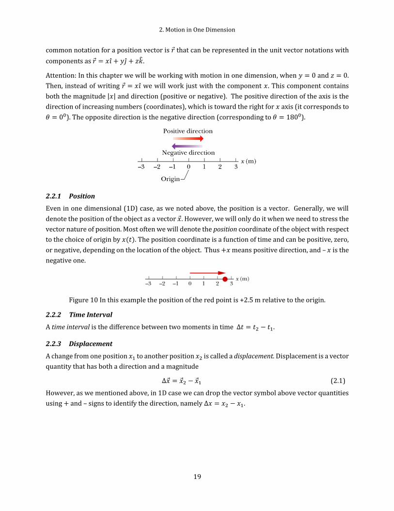
Attention: In this chapter we will be working with motion in one dimension, when 𝑦 = 0 and 𝑧 = 0.
Then, instead of writing 𝑟 = 𝑥𝑖 ̂we will work just with the component 𝑥. This component contains
both the magnitude |𝑥| and direction (positive or negative). The positive direction of the axis is the
direction of increasing numbers (coordinates), which is toward the right for 𝑥 axis (it corresponds to
𝜃 = 00). The opposite direction is the negative direction (corresponding to 𝜃 = 1800).
2.2.1 Position
Even in one dimensional (1D) case, as we noted above, the position is a vector. Generally, we will
denote the position of the object as a vector �⃗�. However, we will only do it when we need to stress the
vector nature of position. Most often we will denote the position coordinate of the object with respect
to the choice of origin by 𝑥(𝑡). The position coordinate is a function of time and can be positive, zero,
or negative, depending on the location of the object. Thus +𝑥 means positive direction, and – 𝑥 is the
negative one.
Figure 10 In this example the position of the red point is +2.5 m relative to the origin.
2.2.2 Time Interval
A time interval is the difference between two moments in time Δ𝑡 = 𝑡2 − 𝑡1.
2.2.3 Displacement
A change from one position 𝑥1 to another position 𝑥2 is called a displacement. Displacement is a vector
quantity that has both a direction and a magnitude
Δ�⃗� = �⃗�2 − �⃗�1 (2.1)
However, as we mentioned above, in 1D case we can drop the vector symbol above vector quantities
using + and – signs to identify the direction, namely Δ𝑥 = 𝑥2 − 𝑥1.

2.3 Velocity and Speed
20
Figure 11 Positions of an object at two times 𝑡1 and 𝑡2 and its displacement
Note the importance of the sign, for example for 𝑥1 = 5 and 𝑥2 = +7 the displacement is +7 − 5 =
2, but for 𝑥1 = 5 and 𝑥2 = −7 the displacement is −7 − (5) = −12.
Attention: in physics “displacement” and “distance” have different definitions. Thus, “distance” is a
scalar and means the total ground covered while traveling, e.g. odometer reading, but the
“displacement” is a vector from where you started to where you end up.
Results of observations of motions can be conveniently presented as a table, or by means of a graph.
Figure 12 Example of 1D motion (position as a function of time)
2.3 Velocity and Speed
The terms velocity and speed are often used interchangeably in ordinary language. But introducing a
mathematical description of motion we make a clear distinction between the two.
The term "speed" refers to how far an object travels in a given time interval regardless of direction. If
a car travels 240 kilometers (km) in 3 hours, we say its average speed was 80 km/h.
In general; the average speed of an object is defined as
𝑠𝑎𝑣𝑔 =𝑡𝑜𝑡𝑎𝑙 𝑑𝑖𝑠𝑡𝑎𝑛𝑐𝑒
𝑡2 − 𝑡1 (2.2)
Because average speed does not include direction, it lacks any algebraic sign, i.e. it is always positive.
The average velocity is a vector defined as “how fast”, or the displacement divided by the time
interval

2. Motion in One Dimension
21
�⃗�𝑎𝑣𝑔 =Δ�⃗�
Δ𝑡=
�⃗�2 − �⃗�1
𝑡2 − 𝑡1. (2.3)
Again, as we mentioned above, in 1D case we can drop the vector symbol above vector quantities
using + and – signs to identify the direction, thus in this chapter we can use
𝑣𝑎𝑣𝑔 =Δ𝑥
Δ𝑡=
𝑥2 − 𝑥1
𝑡2 − 𝑡1 (2.4)
as the definition for average velocity.
The average velocity can be even equal to zero if an object ended up in the same position where it
started. For example, driving from home to a class and later coming back home will result in zero
displacement thus giving zero average velocity.
Figure 13 Calculation of average velocity
Note: Sometimes 𝑠𝑎𝑣𝑔 is the same (except for the absence of sign) as 𝑣𝑎𝑣𝑔. However, when an object
doubles back on its path the two can be quite different.
Figure 14 Average velocity at different time intervals.
2.4 Acceleration
22
In example above (Figure 14) the red, blue, and green straight lines represent the object motion as if
it was moving at constant average velocity (equation (2.4)) for different time intervals. So, for various
time intervals we get 𝑣27 = 9 𝑚/𝑠, 𝑣25 = 7 𝑚/𝑠, 𝑣23 = 5 𝑚/𝑠. As the time interval becomes
smaller, the lines that represent those average velocities approach the tangent to the curve at the time
of interest 𝑡 = 2 𝑠 and 𝑣22 = 4 𝑚/𝑠.
The definitions of average speed or average velocity look as simple ones, but there are indeed some
subtleties in reasoning about speed.
Example: At the point where an old lady in the car is caught by a cop, the cop comes up to her and
says, "Lady, you were going 60 miles an hour!" She says, "That's impossible, sir, I was travelling for
only seven minutes. It is ridiculous - how can I go 60 miles an hour when I wasn't going an hour?"
How would you answer her if you were the cop?
The instantaneous velocity is a vector defined as “how fast” a particle is moving at a given instant.
�⃗�(𝑡) = limΔ𝑡→0
Δ�⃗�
Δ𝑡= lim
Δ𝑡→0
�⃗�(𝑡 + Δ𝑡) − �⃗�(𝑡)
Δ𝑡=
𝑑�⃗�
𝑑𝑡 (2.5)
Yet again, in 1D case we can drop vector notations using + and – for directions, then we can write
𝑣(𝑡) = limΔ𝑡→0
Δ𝑥
Δ𝑡= lim
Δ𝑡→0
𝑥(𝑡 + Δ𝑡) − 𝑥(𝑡)
Δ𝑡=
𝑑𝑥
𝑑𝑡 (2.6)
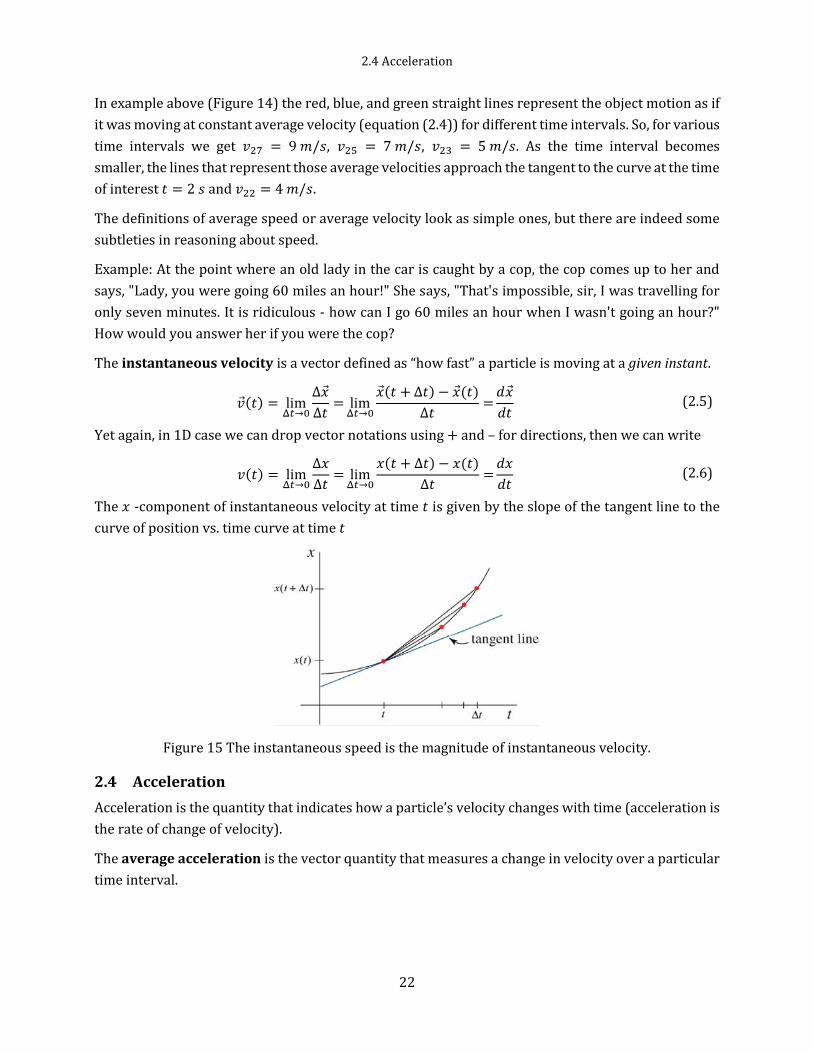
The 𝑥 -component of instantaneous velocity at time 𝑡 is given by the slope of the tangent line to the
curve of position vs. time curve at time 𝑡
Figure 15 The instantaneous speed is the magnitude of instantaneous velocity.
2.4 Acceleration
Acceleration is the quantity that indicates how a particle’s velocity changes with time (acceleration is
the rate of change of velocity).
The average acceleration is the vector quantity that measures a change in velocity over a particular
time interval.

2. Motion in One Dimension
23
�⃗�𝑎𝑣𝑔 =�⃗�2 − �⃗�1
𝑡2 − 𝑡1=
Δ�⃗�
Δ𝑡 (2.7)
The instantaneous acceleration (or simply acceleration) is the derivative of the velocity with
respect to time
�⃗� = limΔ𝑡→0
Δ�⃗�
Δ𝑡= lim
Δ𝑡→0
�⃗�(𝑡 + Δ𝑡) − �⃗�(𝑡)
Δ𝑡=
𝑑�⃗�
𝑑𝑡=
𝑑
𝑑𝑡(
𝑑�⃗�
𝑑𝑡) =
𝑑2�⃗�
𝑑𝑡2 (2.8)
or we can write it as
�⃗� =𝑑�⃗�
𝑑𝑡=
𝑑2�⃗�
𝑑𝑡2 (2.9)
Note that here we could write the second set of equations for 1D case, now without vectors, like we
did before.
Figure 16 Instantaneous acceleration
A common unit of acceleration is meter per second per second: 𝑚/(𝑠𝑠) or 𝑚/𝑠2. Large accelerations
are sometimes expressed in terms of 𝑔 units, with = 9.8 𝑚 𝑠2⁄ . Soon we will see that 𝑔 is the free-fall
acceleration.
Attention: Acceleration and velocity may have the same or different signs! If the signs are the same
then an object is speeding up; if the signs are different, then an object is slowing down.
Example: The positions of two cars at successive 1.0-second time intervals are represented in the
figures below.
What can conclude about the car’s speed and acceleration for the first car?
What can conclude about the car’s speed and acceleration for the second car?

2.5 Motion with constant velocity
24
2.5 Motion with constant velocity
Let’s consider a simple type of motion when the velocity is constant (e.g. driving a car with 55 mph in
the same direction). The acceleration is equal to zero in this case, i.e. 𝑎 = 0. When the velocity is
constant, the average and instantaneous velocity are equal, and we can write with some change in
notations as
𝑣 = 𝑣𝑎𝑣𝑔 =𝑥 − 𝑥0
𝑡 − 0 (2.10)
Here 𝑥0 is the position at time 𝑡 = 0, and 𝑥 is the position at any later time 𝑡. We can recast this
equation as
𝑥 = 𝑥0 + 𝑣𝑎𝑣𝑔𝑡 (2.11)
As one can see, the position is a linear function of the time
Figure 17 Position as a function of time for notion with constant velocity (𝑎 = 0).
2.6 Motion with constant acceleration
Many practical situations occur in which the acceleration is constant or close enough that we can
assume it is constant. For example, a car accelerating after a traffic light turns green, a taking off
airplane, or a falling body. In this case, the velocity changes with constant rate.
Let’s recall definitions for the instantaneous velocity and acceleration
𝑣 =𝑑𝑥
𝑑𝑡 (2.12)
𝑎 =𝑑𝑣
𝑑𝑡 (2.13)
The first equation (2.12) can be written as 𝑑𝑥 = 𝑣𝑑𝑡 and the second equation (2.13) as 𝑑𝑣 = 𝑎𝑑𝑡.
Integrating both sides of the second equation gives ∫ 𝑑𝑣 = ∫ 𝑎𝑑𝑡 with 𝑣 = 𝑎𝑡 + 𝐶1. Since at time 𝑡 =
0 𝐶1 = 𝑣0 then we can write
𝑣 = 𝑣0 + 𝑎𝑡

2. Motion in One Dimension
25
Now we integrate the first equation ∫ 𝑑𝑥 = ∫ 𝑣𝑑𝑡 with the equation above for the velocity ∫ 𝑑𝑥 =
∫(𝑣0 + 𝑎𝑡)𝑑𝑡 to get
𝑥 = 𝑣0𝑡 +𝑎𝑡2
2+ 𝐶2
From the initial condition 𝑥 = 𝑥0 at 𝑡 = 0 follows 𝐶2 = 𝑥0, then
𝑥 = 𝑥0 + 𝑣0𝑡 +𝑎𝑡2
2
Thus, everything we need to know to describe motion under constant acceleration is contained in just
two simple equations (everything else you may need for solving problems can be derived from these
equation using algebra!)
𝑥(𝑡) = 𝑥0 + 𝑣0𝑡 +𝑎𝑡2
2 (2.14)
𝑣(𝑡) = 𝑣0 + 𝑎𝑡 (2.15)
These equations are the basic equations for motion with constant acceleration. Reiterating again, these
equations can be used to solve any constant acceleration problem in case of 1D motion.
Attention: You need to have at least as many equations as unknown variables to find a unique solution.
The two above equations can only be solved if there are only two unknown variables.
Just as a reminder, these two equation use 𝑡0 = 0 as the reference time, so the variable 𝑡0 does not
appear in either case.
The figures below shows the position, velocity and (constant) acceleration as a function of time
The position 𝑥(𝑡) of a particle moving with constant acceleration
Its velocity 𝑣(𝑡) given at each point by the slope of the curve in (a)
Its (constant) acceleration, equal to the (constant) slope of the curve of 𝑣(𝑡)

2.6 Motion with constant acceleration
26
Let’s consider contributions of every term in equation for position 𝑥 and velocity 𝑣
Figure 18 Contributions of terms for𝑥 when 𝑥0 = 10 𝑚, 𝑣0 = 2 𝑚 ⁄ 𝑠 and 𝑎 = 1 𝑚 ⁄ 𝑠2.
Figure 19 Velocity as a function of time 𝑣 = 𝑣0 + 𝑎𝑡 (for 𝑣0 = 2 𝑚 ⁄ 𝑠 and𝑎 = 1 𝑚 ⁄ 𝑠2 )

2. Motion in One Dimension
27
Attention: Deceleration does not mean the acceleration is negative. A deceleration results in an
object’s speed decreasing in magnitude. An object is decelerating – slowing down – when its
acceleration and velocity have opposite signs. Here are two examples.
Example 1: where 𝑣0 = 1 𝑚 𝑠⁄ , and 𝑎 = 1 𝑚 𝑠2⁄ have the same sign (direction)
Example 2: where initially velocity and acceleration have opposite signs
𝑣0 = −6 𝑚 𝑠⁄ , 𝑎 = +1 𝑚 𝑠2⁄ (note that after 𝑡 = 6 𝑠 the velocity has the same sign as acceleration)
2.7 Freely Falling Bodies
28
It is often useful to have a relationship between position, velocity and (constant) acceleration that
does not involve the time. To obtain this we first solve the first basic equation for time
𝑡 =𝑣 − 𝑣0
𝑎
and then substitute the result into the second equation
𝑥 = 𝑥0 + 𝑣0 (𝑣 − 𝑣0
𝑎) +
1
2𝑎 (
𝑣 − 𝑣0
𝑎)
2
2𝑎(𝑥 − 𝑥0) = 2𝑣0𝑣 − 2𝑣02 + 𝑣2 − 2𝑣𝑣0 + 𝑣0
2
and finally
𝑣2 = 𝑣02 + 2𝑎(𝑥 − 𝑥0) (2.16)
This equation is useful if we do not know 𝑡 and are not required to find it (𝑡 can be called a “missing
variable” in this case).
We can also eliminate the acceleration from the basic equations (2.14) and (2.15) to produce an
equation in which acceleration 𝑎 does not appear (𝑎 is a “missing variable”)
𝑥 − 𝑥0 =1
2(𝑣0 + 𝑣)𝑡 (2.17)
The power of physics is in generalization of complicated phenomena with one or only a few equations
in terms of small number of variables. Here we have our first example of that capability. Just TWO
equations describe all one dimensional motion with constant accelerations.
SUMMARY: Let’s write again the two basic equations describing 1D motion of a particle with constant
acceleration
𝑥(𝑡) = 𝑥0 + 𝑣0𝑡 +𝑎𝑡2
2 (2.18)
𝑣(𝑡) = 𝑣0 + 𝑎𝑡 (2.19)
together with the two auxiliary equations that are easily derived from the equations above, namely
𝑣2 = 𝑣02 + 2𝑎(𝑥 − 𝑥0) (2.20)
𝑥 − 𝑥0 =1
2(𝑣0 + 𝑣)𝑡
(2.21)
2.7 Freely Falling Bodies
The most familiar example of motion with (nearly) constant acceleration is a body falling under the
influence of the earth's gravitational attraction. Such motion has held the attention of philosophers
and scientists since ancient times. In the fourth century B.C., Aristotle thought (erroneously) that
heavy bodies fall faster than light bodies, in proportion to their weight. Nineteen centuries later,

2. Motion in One Dimension
29
Galileo argued that a body should fall with a downward acceleration that is constant and independent
of its weight.
Experiment shows that if the effects of the air can be neglected, Galileo is right; all bodies at a
particular location fall with the same downward acceleration, regardless of their size or weight.
If in addition the distance of the fall is small compared with the radius of the earth, and if we ignore
small effects due to the earth's rotation, the acceleration is constant. The idealized motion that results
under all of these assumptions is called free fall, although it includes rising as well as falling motion.
The constant acceleration of a freely falling body is called the acceleration due to gravity, and we
denote its magnitude with the letter g. We will frequently use the approximate value of g at or near
the earth's surface: g = 9.8 m/s2.
The exact value varies with location, so we will often give the value of g at the earth's surface to only
two significant figures. Because g is the magnitude of a vector quantity, it is always a positive number.
On the surface of the moon, the acceleration due to gravity is caused by the attractive force of the
moon rather than the earth, and g = l.6 m/s2. Near the surface of the sun, g = 270 m/s2.
Attention: Objects accelerate downward under the influence of gravity, but the value of g is positive.
Accordingly, the equations for the freely falling bodies are easily written using (2.18) for the position
𝑦(𝑡) = 𝑦0 + 𝑣0𝑡 −𝑔𝑡2
2 (2.22)
and (2.19) for the velocity
𝑣(𝑡) = 𝑣0 − 𝑔𝑡 (2.23)
with a quite practical auxiliary equation
𝑣2 = 𝑣02 − 2𝑔(𝑦 − 𝑦0) (2.24)
Here is a link to a wonderful experiment -free fall for a hammer and a feather on the moon
http://www.youtube.com/watch?v=5C5_dOEyAfk

2.7 Freely Falling Bodies
30
Example: position, velocity and acceleration as functions of time for 𝑣0 = 10 𝑚 𝑠⁄ , 𝑔 = 9.8 𝑚 𝑠2⁄

2. Motion in One Dimension
31
2.8 Most common problems
Most problems in introductory physics on one dimensional motion can be classified as
Case 1: One object, one time interval
Then all we need is the two basic equations
𝑥 = 𝑥0 + 𝑣0𝑡 +𝑎𝑡2
2
𝑣 = 𝑣0 + 𝑎𝑡
Remember that the two auxiliary equations (2.20) and (2.21) are easily derived from the basic
equations.
Case 2: One object, two time intervals
In this case we use the basic equations two times, first for the first time interval, and later for the
second interval, where the results from the first interval are the initial conditions for the second
interval. This for the first interval (from time 𝑡0 to time 𝑡1)
𝑥1 = 𝑥0 + 𝑣0𝑡1 +𝑎0𝑡1
2
2
𝑣1 = 𝑣0 + 𝑎0𝑡1
and then for the second interval (from time 𝑡1 to time 𝑡2)
𝑥2 = 𝑥1 + 𝑣1𝑡2 +𝑎1𝑡2
2
2
𝑣2 = 𝑣1 + 𝑎1𝑡2
Case 3: Two objects, one time interval
Then we have a system of equations for two objects that share the same time
𝑥1 = 𝑥01 + 𝑣01𝑡 +𝑎1𝑡2
2
𝑣1 = 𝑣01 + 𝑎1𝑡
𝑥2 = 𝑥02 + 𝑣02𝑡 +𝑎2𝑡2
2
𝑣2 = 𝑣02 + 𝑎2𝑡
There are very many variations for “two object problems”. As a rule solutions can be derived from the
equations above (after some simple algebra).
One of examples for such problems is a “collision” problem, when one object chases a second object,
and later they are at the same point in space (𝑥1 = 𝑥2) at the same moment in time 𝑡𝑐.
𝑥01 + 𝑣01𝑡𝑐 +𝑎1𝑡𝑐
2
2= 𝑥02 + 𝑣02𝑡𝑐 +
𝑎2𝑡𝑐2
2
Generally, time 𝑡𝑐 is unknown, and you need to solve quadratic equations to find it

2.9 Examples
32
𝑎2 − 𝑎1
2𝑡𝑐
2 + (𝑣20 − 𝑣10)𝑡𝑐 + (𝑥02 − 𝑥01) = 0
If the initial separation between two objects is zero 𝑥02 − 𝑥01 = 0, then you solve a linear equation.
2.9 Examples
Example 2-1
The catapult of the aircraft carrier USS Abraham Lincoln accelerates an F/A-18 Hornet jet fighter from
rest to a takeoff speed of 173 mph in a distance of 307 ft. Assume constant acceleration.
a) Calculate the acceleration of the fighter in m/s.
b) Calculate the time required for the fighter to accelerate to takeoff speed.
SOLUTION:
1. Physics – one-dimensional motion with constant acceleration for one object and one time interval
2. The basic equations for 1D motion with constant acceleration
𝑥 = 𝑥0 + 𝑣0𝑡 +𝑎𝑡2
2
𝑣 = 𝑣0 + 𝑎𝑡
3. Using given data 𝑥0 = 0 𝑚 and 𝑣0 = 0 𝑚/𝑠 , we may rewrite the basic equations as
𝑥 =𝑎𝑡2
2
𝑣 = 𝑎𝑡
4. There are two unknowns in the system above, namely the acceleration 𝑎 and the time 𝑡. From the
second equation we have 𝑡 = 𝑣/𝑎. Substituting it into the first equation gives
𝑥 =1
2∙ 𝑎 ∙
𝑣2
𝑎2=
𝑣2
2𝑎, 𝑡ℎ𝑒𝑛 𝑎 =
𝑣2
2𝑥,
using this solution with 𝑡 = 𝑣/𝑎
𝑡 =𝑣
𝑎= 𝑣 ∙
2𝑥
𝑣2=
2𝑥
𝑣
Now we have two analytic solutions for the unknowns.
5. Calculations:
The initial data in SI units (we use 1 ft = 0.3048 m, 1 mile = 1609 m, 1 h = 3600 s)

2. Motion in One Dimension
33
307 𝑓𝑡 = 307 𝑓𝑡 (0.3048 𝑚
1 𝑓𝑡) = 93.6 𝑚
173 𝑚𝑝ℎ = 173 𝑚𝑖𝑙𝑒
ℎ(
1609 𝑚
1 𝑚𝑖𝑙𝑒) (
1 ℎ
3600 𝑠) = 77.3 𝑚/𝑠
calculations
𝑎 =𝑣2
2𝑥=
(77.3 𝑚 𝑠⁄ )2
2 × 93.6 𝑚= 31.9 𝑚 𝑠2⁄ , 𝑡 =
2𝑥
𝑣=
2 × 93.6 𝑚
77.3 𝑚/𝑠 = 2.42 𝑠
6. Let’s evaluate the answer.
Units and dimensions:
𝑎 =𝑣2
2𝑥→ [
𝑚2
𝑠2∙
1
𝑚] = [
𝑚
𝑠2] 𝑂𝐾! 𝑡 =2𝑥
𝑣→ [𝑚 ∙
𝑠
𝑚] = [𝑠] 𝑂𝐾!
Both the time and acceleration have proper units and dimensions.
The takeoff time 𝑡 = 2.42 𝑠 looks as a reasonable numerical value.
Example 2-2
You are driving down the highway late one night at 58 mph when a deer steps into the road 50 m
(about 164 ft) in front of you. Your reaction time before stepping on the brakes is 0.5 s, and the
maximum deceleration of your car is 9.1 m/s2. How much distance is between you and the deer when
you come to stop?
SOLUTION:
1. Physics – one-dimensional motion with constant acceleration for one object but two time intervals
2. The basic equations for 1D motion with constant acceleration
𝑥 = 𝑥0 + 𝑣0𝑡 +𝑎𝑡2
2
𝑣 = 𝑣0 + 𝑎𝑡
3. Note that we have two phases of the motion
Phase 1: “thinking distance” or travelling with constant speed during the reaction time 𝑡1
𝑥1 = 𝑣0𝑡1
Phase 2: “braking distance” or motion with constant deceleration
𝑥2 = 𝑣0𝑡2 −𝑎𝑡2
2
2
0 = 𝑣0 − 𝑎𝑡2

2.9 Examples
34
From the last two equations
𝑥2 =𝑣0
2
2𝑎
4. The total stopping distance
𝑥 = 𝑥1 + 𝑥2 = 𝑣0𝑡1 +𝑣0
2
2𝑎
5. Calculations
58 𝑚𝑝ℎ = 55 𝑚𝑖𝑙𝑒
ℎ(
1609 𝑚
1 𝑚𝑖𝑙𝑒) (
1 ℎ
3600 𝑠) = 25.92 𝑚/𝑠
𝑥 = 25.92 𝑚 𝑠⁄ ∙ 0.5 𝑠 +(25.92 𝑚 𝑠⁄ )2
2 ∙ 9.8 𝑚 𝑠2⁄= 49.9 𝑚
So the car stopped 0.1 𝑚 in front of the deer.
6. We have got both proper dimensions and reasonable numerical results.
Example 2-3
A car speeding at 90 mph passes a still police car which immediately takes off in hot pursuit. Assume
that the speeder continues at a constant speed but the police car moves with constant acceleration.
The technical specification states the police car can accelerate from 0 mph to 60 mph in 8.7 s.
a) How long would it take for the police car to overtake the speeder?
b) Estimate the distance (in meters and miles) of the hot pursuit.
c) Estimate the police car’s speed at that moment the police car overtakes the speeder.
SOLUTION
1. Physics – one dimensional motion with constant acceleration for two objects
2. The basic equations (for two objects)
𝑥1 = 𝑥10 + 𝑣10𝑡 +𝑎1𝑡2
2 𝑥2 = 𝑥20 + 𝑣20𝑡 +
𝑎2𝑡2
2
𝑣1 = 𝑣10 + 𝑎1𝑡 𝑣2 = 𝑣20 + 𝑎2𝑡
Here we call index 1 for the first object (let it be the speeder), and index 2 for the second object (the
police car)
3. The basic equation can be simplified using given data and conditions, namely
The data
at initial time 𝑡 = 0 both cars have the same position 𝑥10 = 0 𝑚, 𝑥20 = 0 𝑚
the speeder keeps moving with a constant speed, i.e. 𝑎1 = 0 𝑚/𝑠2
the police cars is initially at rest, i.e. 𝑣20 = 0 𝑚/𝑠

2. Motion in One Dimension
35
The condition (the police car overtakes the speeder)
at some time 𝑡 = 𝑡𝑓 both cars are at the same position on the road, i.e. 𝑥1 = 𝑥2
Then the original basic equations can be written as
𝑥1 = 𝑣10𝑡 𝑥2 =𝑎2𝑡2
2
𝑣1 = 𝑣10 𝑣2 = 𝑎2𝑡
4. Using the condition 𝑥1 = 𝑥2 we have
𝑣10𝑡 =𝑎2𝑡2
2
The last equation has two unknowns, namely 𝑡 and 𝑎2. The acceleration of the police car can be found
from the given data (the police car can accelerate from 0 mph to 60 mph in 8.7 s) using the definition
for the average acceleration
𝑎𝑎𝑣𝑔 =Δ𝑣
Δ𝑡
Then solving the equation 𝑣10𝑡 =𝑎2𝑡2
2 for the unknown time we get
𝑡 =2𝑣10
𝑎2
Having the time, we can easily find the distance of the hot pursuit
𝑥1 = 𝑣10 ∙2𝑣10
𝑎2=
2𝑣102
𝑎2 𝑜𝑟 𝑥2 =
𝑎2𝑡2
2=
𝑎2
2∙
22 ∙ 𝑣102
𝑎2=
2𝑣102
𝑎2 (𝑡ℎ𝑒 𝑠𝑎𝑚𝑒 𝑎𝑠 𝑥1)
Thus
𝑥 =2𝑣10
2
𝑎2
Using 𝑣2 = 𝑎2𝑡 we get
𝑣2 = 𝑎2 ∙2𝑣10
𝑎2= 2𝑣10
𝑣2 = 2𝑣10
5. Calculations
First we should switch to SI units using: 1 mile = 1609 m, 1 h = 3600 s
90 𝑚𝑝ℎ = 90 𝑚𝑖𝑙𝑒
ℎ(
1609 𝑚
1 𝑚𝑖𝑙𝑒) (
1 ℎ
3600 𝑠) = 40 𝑚/𝑠

2.9 Examples
36
60 𝑚𝑝ℎ = 60 𝑚𝑖𝑙𝑒
ℎ(
1609 𝑚
1 𝑚𝑖𝑙𝑒) (
1 ℎ
3600 𝑠) = 27 𝑚/𝑠
The police car acceleration
𝑎2 =27 𝑚 𝑠⁄ − 0 𝑚 𝑠⁄
8.7 𝑠= 3.1 𝑚 𝑠2⁄
𝑡 =2𝑣10
𝑎2=
2 ∙ 40 𝑚/𝑠
3.1 𝑚 𝑠2⁄= 26 𝑠
𝑥 =2𝑣10
2
𝑎2=
2 ∙ (40 𝑚/𝑠)2
3.1 𝑚 𝑠2⁄= 1030 𝑚
𝑣2 = 2𝑣10 = 80 𝑚/𝑠
6. Let’s evaluate the results
The dimensions and units are correct.
Both the time and distance of the pursuit seem realistic.
How about the speed of the police car? Since we are more comfortable with mph or km/h we can
write that 80 𝑚 𝑠⁄ = 180 𝑚𝑝ℎ. This is very high (and risky) speed! It is rather unlikely that an average
police car can go so fast (unless it is a Ferrari or Lamborghini).
Despite the numerical solutions seem correct, in real life different pursuit tactics should be used
(decreasing the acceleration when the speed is above 100 mph that would result in a longer pursuit
time, or calling for a roadblock ahead of the speeder, etc.).
Example 2-4
The engineer of a passenger train traveling at 30.0 m/s sights a freight train whose caboose is 100 m
ahead on the same track. The freight train is traveling at 15.0 m/s in the same direction as the
passenger train. The engineer of the passenger train immediately applies the brakes, causing a
constant acceleration of -1.0 m/s2, while the freight train continues with constant speed.
a) Will the cows nearby witness a collision? If so, determine how far from the initial position of
the passenger train and at what time the collision occurs.
b) If not, determine the distance of closest approach between two trains
SOLUTION
1. Physics – one dimensional motion with constant acceleration for two objects
2. The basic equations (for two objects)
𝑥1 = 𝑥10 + 𝑣10𝑡 +𝑎1𝑡2
2 𝑥2 = 𝑥20 + 𝑣20𝑡 +
𝑎2𝑡2
2
𝑣1 = 𝑣10 + 𝑎1𝑡 𝑣2 = 𝑣20 + 𝑎2𝑡

2. Motion in One Dimension
37
Here we call index 1 for the passenger train, and index 2 for the cargo train
3. The basic equation can be simplified using given data and conditions, namely
The data
at initial time 𝑡 = 0 the passenger train is at 𝑥10 = 0 but the freight train is at 𝑥20
the freight train moves with a constant speed, i.e. 𝑎2 = 0
The condition (a collision)
at some time 𝑡 = 𝑡𝑓 both trains are at the same position i.e. 𝑥1 = 𝑥2
Then the original basic equations for the positions can be written as
𝑥1 = 𝑣10𝑡 +𝑎1𝑡2
2 𝑥2 = 𝑥20 + 𝑣20𝑡
4. Using the condition 𝑥1 = 𝑥2 we have
𝑣10𝑡 +𝑎1𝑡2
2= 𝑥20 + 𝑣20𝑡,
𝑎1𝑡2
2+ (𝑣10 − 𝑣20)𝑡 − 𝑥20 = 0
This is a quadratic equation for 𝑡.
5. Calculations
Solving the equation for 𝑎 = −1.0 𝑚/𝑠2, 𝑣10 − 𝑣20 = 15 𝑚/𝑠, and 𝑥20 = 100 𝑚 gives two solutions
𝑡1 = 10.0 𝑠, 𝑡2 = 20.0 𝑠. The first solutions corresponds to the collision. If the trains were travelling
on parallel tracks, the second solution would correspond for the trains to run parallel again.
For 𝑡1 = 10.0 𝑠 the position of the trains (relative to the point where the engineer of the passenger
train saw the problem 𝑥10 = 0) is 𝑥1 = 250 𝑚
6. Let’s evaluate the results
Both the time and distance of the pursuit seem realistic.
Attention. If solving quadratic equation for time 𝑡 you are getting complex roots (i.e. a negative number
under square root) then there is no collision between the objects. In this case the distance between the
trains as a function of time is
𝑥2 − 𝑥1 = 𝑥20 + 𝑣20𝑡 − 𝑣10𝑡 −𝑎1𝑡2
2
Differentiating over time 𝑡 and setting 𝑑(𝑥2 − 𝑥1)/𝑑𝑡 = 0 gives equation to find the time for the
closest approach
𝑑(𝑥2 − 𝑥1)
𝑑𝑡= 𝑣20 − 𝑣10 − 𝑎1𝑡 = 0, 𝑡 =
𝑣10 − 𝑣20
𝑎1
As one can see, at such distance the velocities of both trains are equal, or 𝑣10 + 𝑎1𝑡 = 𝑣20. Having this
time you can easily find the distance of the closest approach between two trains.

2.9 Examples
38
Example 2-5
An apple (a fruit or a computer) is dropped from a bridge that is 52.0 m above the river. Neglecting
air resistance
a) How long does the apple take to reach the water?
b) What is its speed just as it strikes the water surface?
SOLUTION:
1. Physics – one-dimensional motion vertical with constant free-fall acceleration (𝑎 = −𝑔)
2. The basic equations
𝑦 = 𝑦0 + 𝑣0𝑡 −𝑔𝑡2
2
𝑣 = 𝑣0 − 𝑔𝑡
3. The basic equations can be simplified using the given conditions (𝑣0 = 0, 𝑦 = 0). (We choose the
river surface as our zero level). Then
0 = 𝑦0 −𝑔𝑡2
2
𝑣 = −𝑔𝑡
4. Solving the first equation gives the time
𝑡 = √2𝑦0
𝑔
then from the second equation
𝑣 = −𝑔 ∙ √2𝑦0
𝑔= −√2𝑦0𝑔
5. Calculations
𝑡 = √2𝑦0
𝑔= √
2 ∙ 52 𝑚
9.8 𝑚 𝑠2⁄= 3.26 𝑠 𝑣 = −√2𝑦0𝑔 = −√2 ∙ 52 𝑚 ∙ 9.8 𝑚 𝑠2⁄ = −31.9 𝑚 𝑠⁄
6. The time looks reasonable (from experience). We certainly have correct units for both time and
velocity.

2. Motion in One Dimension
39
Example 2.6
If the apple was thrown vertically upward from the same bridge with a speed of 10.0 m/s
a) How high above its starting point would the apple go?
b) In how many seconds after being thrown upward would the apple strike the water below?
SOLUTION:
1. Physics – one-dimensional motion vertical with constant free-fall acceleration
2. The basic equations
𝑦 = 𝑦0 + 𝑣0𝑡 −𝑔𝑡2
2
𝑣 = 𝑣0 − 𝑔𝑡
3-4. The problem has two parts, namely motion to the highest point, and total motion to the river.
a) For the first part the basic equations can be rewritten as
𝑦𝑡𝑜𝑝 = 𝑦0 + 𝑣0𝑡 −𝑔𝑡2
2
0 = 𝑣0 − 𝑔𝑡
The first equation has two unknowns, but the second equation has only one unknown. Solving the
second equation gives the time to the top point
𝑡 = 𝑣0/𝑔
Using this time in the first equation provides the distance
𝑦𝑡𝑜𝑝 = 𝑦0 + 𝑣0
𝑣0
𝑔−
𝑔
2
𝑣02
𝑔2= 𝑦0 +
1
2
𝑣02
𝑔
thus, from the bridge the apple goes as high as
Δ𝑦 =𝑣0
2
2𝑔
b) For the second part the final vertical position is zero (the river)
0 = 𝑦0 + 𝑣0𝑡 −𝑔𝑡2
2
𝑣 = 𝑣0 − 𝑔𝑡
The first equation has only one unknown, namely the time that we are looking for. This is a quadratic
equation.
5. Calculations

2.9 Examples
40
𝑎) Δ𝑦 =𝑣0
2
2𝑔=
(10 𝑚 𝑠⁄ )^2
2 ∙ 9.8 𝑚 𝑠2⁄ = 5.10 𝑚
b) the quadratic equation has two solutions, 𝑡1 = −2.39 𝑠, 𝑡2 = 4.43 𝑠.
Out of two solutions only the second satisfies the given conditions that the apple hits the water after
it was thrown from the bridge. The first solution satisfies another condition that the apple was at the
river level before it reached the bridge with the given speed. This could happen if the apple was
thrown from the water surface with an appropriate velocity.
6. The time looks reasonable (a bit large time when the apple was thrown upward). We certainly have
correct units for both time and speed.
Example 2-7
A 75-kg person jumps from a fourth-story window 15.0 m above a
firefighter's safety net. The survivor stretches the net 1.0 m before
coming to rest,
a) How long was the survivor in free fall?
b) What was his speed just as he reached the net?
c) What was the average deceleration experienced by the
survivor on the net (in g units)?
d) What would you do to make it “safer” (that is to generate a
smaller deceleration)? Would you stiffen or loosen the net?
Explain.
e) How would your answers change if it was a 1,500 kg
hippopotamus?
SOLUTION
1. Physics – one dimensional motion with constant acceleration
2. The basic equations for 1D motion with constant acceleration
𝑦 = 𝑦0 + 𝑣0𝑡 −𝑔𝑡2
2
𝑣 = 𝑣0 − 𝑔𝑡
3. From the given information follows that we have two phases of motion, the first one is from the
window to the net, and the second one is the stopping by stretching the net. Let’s call the window as
the initial position. The net is located at level 1, and the end position is at level 2. Then the velocity at
the end of the first phase is the initial velocity for the second phase. Since the initial velocity was
0 𝑚/𝑠, and the final velocity at level 2 was 𝑣2 = 0 𝑚/𝑠,
then for the first phase of motion

2. Motion in One Dimension
41
𝑦1 = 𝑦0 −𝑔𝑡1
2
2𝑣1 = −𝑔𝑡1
and for the second phase of motion
𝑦2 = 𝑦1 + 𝑣1𝑡2 +𝑎2𝑡2
2
2∙ 𝑣2 = 0 = 𝑣1 + 𝑎2𝑡2
4. We can easily solve the first set of equation to find both the time 𝑡1 and velocity 𝑣1
𝑡1 = √2(𝑦0 − 𝑦1)
𝑔 𝑎𝑛𝑑 𝑣1 = −𝑔√
2(𝑦0 − 𝑦1)
𝑔= √2(𝑦0 − 𝑦1)𝑔
Now we consider the second set of equations. From 0 = 𝑣1 + 𝑎2𝑡2 we have 𝑡2 = − 𝑣1 𝑎2⁄ (it looks like
we have a problem here with negative time, but remember that 𝑣1 is negative!). Then the first
equation reads
𝑦2 − 𝑦1 = 𝑣1𝑡2 +𝑎2𝑡2
2
2= 𝑣1 (−
𝑣1
𝑎2) +
𝑎2
2
𝑣12
𝑎22 = −
𝑣12
𝑎2+
𝑣12
2𝑎2= −
𝑣12
2𝑎2 𝑜𝑟 𝑣1
2 = 2𝑎2(𝑦1 − 𝑦2) 𝑎𝑛𝑑 𝑎2
=𝑣1
2
2(𝑦1 − 𝑦2)
At this moment we can write analytic solutions for all questions
(a) How long was the survivor in free fall?
𝑡1 = √2(𝑦0 − 𝑦1)
𝑔
(b) What was his speed just as he reached the net?
𝑣1 = √2(𝑦0 − 𝑦1)𝑔
(c) What was the average deceleration experienced by the survivor on the net (in terms of gravity
"g")?
𝑎2 =𝑣1
2
2(𝑦1 − 𝑦2)=
2(𝑦0 − 𝑦1)𝑔
2(𝑦1 − 𝑦2)=
(𝑦0 − 𝑦1)
(𝑦1 − 𝑦2)𝑔
(d) What would you do to make it “safer” (that is to generate a smaller deceleration)? Would you
stiffen or loosen the net? Explain
It is clear from the equation for 𝑎2 that increasing the stopping distance (𝑦1 − 𝑦2) will decrease the
deceleration, making safer landing. Therefore, loosening the net will make it "safer".
(e) How would your answers change if it was a 1,500 kg hippopotamus?
All our answer does not depend on mass of an object. Therefore, there results are going to be the same
for any object if the effect of air resistance can be neglected.

2.9 Examples
42
5. Calculations
All the initial data were given in SI units (lucky us)
𝑡1 = √2(𝑦0 − 𝑦1)
𝑔= √
2 ∙ 15 𝑚
9.8 𝑚 𝑠2⁄= 1.7 𝑠
𝑣1 = √2(𝑦0 − 𝑦1)𝑔 = √2 ∙ 15 𝑚 ∙ 9.8 𝑚 𝑠2⁄ = 17 𝑚/𝑠
𝑎2 =(𝑦0 − 𝑦1)
(𝑦1 − 𝑦2)𝑔 =
15 𝑚
1 𝑚𝑔 = 15𝑔
6. Let’s evaluate our results
The dimensions and units are correct.
The free fall time seems right. For evaluating the “landing” speed we may use 𝑚𝑝ℎ units
17 𝑚 𝑠⁄ = 17𝑚
𝑠(
1 𝑚𝑖𝑙𝑒
1609 𝑚) (
3600 𝑠
1 ℎ) = 38 𝑚𝑝ℎ
It looks like a speed one would expect (fast and dangerous).
The deceleration is high 15𝑔 but the number is correct. It means that landing on a safety at given
conditions is probably unpleasant experience.

3. Motion in Two Dimensions
43
3 Motion in Two Dimensions
Knowing the basics of two-dimensional motion will allow us to examine a wide variety of motions,
ranging from a simple projectile motion to the motion of satellites, or orbit to the motion of electrons
in a uniform electric field.
3.1 Position, displacement, velocity and acceleration in 2D and 3D
For motion in two or three dimensions we can extend the ideas from 1D motion for displacement,
velocity and acceleration.
3.1.1 The displacement
Using the vector algebra we may define a position vector 𝑟, which is a vector that extends from a
reference point (usually the origin of a coordinate system) to the particle. In the unit-vector notation,
it can be written
𝑟 = 𝑥𝑖̂ + 𝑦𝑗̂ + 𝑧�̂� (3.1)
where 𝑥𝑖,̂ 𝑦𝑗̂, and 𝑧�̂� are the vector components of 𝑟, and the coefficients 𝑥, 𝑦 and 𝑧 are its scalar
components. The coefficients 𝑥, 𝑦 and 𝑧 give the particle's location along the coordinate axes and
relative to the origin; that is, the particle has the rectangular coordinates (𝑥, 𝑦, 𝑧).
Going from two to three dimension motion is just adding an additional coordinate 𝑧. For clarity we
will mostly concentrate on 2D motion in (𝑥, 𝑦) plane.

3.1 Position, displacement, velocity and acceleration in 2D and 3D
44
As a particle moves, its position vector changes in such a way that the vector always extends to the
particle from the reference point (the origin). If the position vector changes, say, from 𝑟1⃗⃗⃗ ⃗ to 𝑟2⃗⃗⃗⃗ during
a certain time interval, then the particle's displacement Δ𝑟 during that time interval is
Δ𝑟 = 𝑟2⃗⃗⃗⃗ − 𝑟1⃗⃗⃗ ⃗ (3.2)
Using the unit-vector notation, we can rewrite this displacement as
Δ𝑟 = (𝑥2�̂� + 𝑦2𝑗̂) − (𝑥1𝑖̂ + 𝑦1𝑗̂)
or as
Δ𝑟 = (𝑥2 − 𝑥1)𝑖̂ + (𝑦2 − 𝑦1)𝑗̂ (3.3)
where coordinates (𝑥1, 𝑦1) correspond to position vector 𝑟1⃗⃗⃗ ⃗ and coordinates (𝑥2, 𝑦2) correspond to
position vector 𝑟2⃗⃗⃗⃗ . We can also rewrite the displacement by substituting Δ𝑥 = (𝑥2 − 𝑥1) and Δ𝑦 =
(𝑦2 − 𝑦1).
Δ𝑟 = Δ𝑥𝑖̂ + Δ𝑦𝑗̂
3.1.2 The average velocity and instantaneous velocity
If a particle moves through a displacement Δ𝑟 in a time interval Δ𝑡, then its average velocity �⃗�𝑎𝑣𝑔 is
�⃗�𝑎𝑣𝑔 =𝑟2 − 𝑟1
𝑡2 − 𝑡1=
Δ𝑟
Δ𝑡.
This tells us the direction of �⃗�𝑎𝑣𝑔 must be the same as that of Δ𝑟. Using the component form we can
write
�⃗�𝑎𝑣𝑔 =Δ𝑥𝑖̂ + Δ𝑦𝑗̂
Δ𝑡=
Δ𝑥
Δ𝑡𝑖̂ +
Δ𝑦
Δ𝑡𝑗̂ (3.4)
The instantaneous velocity �⃗� is defined as the limit of the average velocity
�⃗� = limΔ𝑡→0
Δ𝑟
Δ𝑡=
𝑑𝑟
𝑑𝑡. (3.5)
That is, the instantaneous velocity equals the derivative of the position vector with respect to time.
The direction of the instantaneous velocity vector at any point in a particle’s path is along a line
tangent to the path at that point and in the direction of motion.
In unit-vector form
�⃗� =𝑑𝑟
𝑑𝑡=
𝑑
𝑑𝑡(𝑥𝑖̂ + 𝑦𝑗̂) =
𝑑𝑥
𝑑𝑡𝑖̂ +
𝑑𝑦
𝑑𝑡𝑗̂ (3.6)
or
�⃗� = 𝑣𝑥𝑖̂ + 𝑣𝑦𝑗 ̂ (3.7)
where the scalar components of �⃗� are
3. Motion in Two Dimensions
45
𝑣𝑥 =𝑑𝑥
𝑑𝑡, 𝑣𝑦 =
𝑑𝑦
𝑑𝑡. (3.8)
3.1.3 Average acceleration and instantaneous acceleration
When a particle's velocity changes from �⃗�1 to �⃗�2in a time interval Δ𝑡, its average acceleration during
Δ𝑡 is
�⃗�𝑎𝑣𝑔 =�⃗�2 − �⃗�1
𝑡2 − 𝑡1=
Δ�⃗�
Δ𝑡 (3.9)
The instantaneous acceleration a is defined as the limiting value of the ratio Δ�⃗�/Δ𝑡, or the
instantaneous acceleration equals the derivative of the velocity vector with respect to time.
�⃗� = limΔ𝑡→0
Δ�⃗�
Δ𝑡=
𝑑�⃗�
𝑑𝑡. (3.10)
Important: If the velocity changes in either magnitude or direction (or both), the particle must have
an acceleration.
In the unit vector notation
�⃗� =𝑑
𝑑𝑡(𝑣𝑥𝑖̂ + 𝑣𝑦𝑗̂) =
𝑑𝑣𝑥
𝑑𝑡𝑖̂ +
𝑑𝑣𝑦
𝑑𝑡𝑗̂ = 𝑎𝑥 �̂� + 𝑎𝑦𝑗̂ (3.11)
where
𝑎𝑥 =𝑑𝑣𝑥
𝑑𝑡, 𝑎𝑦 =
𝑑𝑣𝑦
𝑑𝑡
Thus, we can find the scalar components of �⃗� by differentiating the scalar components of �⃗�.
3.2 Motion with constant acceleration in 2D
Let’s consider a case when acceleration in a plane is constant. In 2D Cartesian coordinates
�⃗� = 𝑎𝑥𝑖̂ + 𝑎𝑦𝑗̂ = 𝑐𝑜𝑛𝑠𝑡1𝑖̂ + 𝑐𝑜𝑛𝑠𝑡2𝑗 ̂
Since in terms of velocity
𝑑𝑣𝑥
𝑑𝑡𝑖̂ +
𝑑𝑣𝑦
𝑑𝑡𝑗̂ = 𝑎𝑥 �̂� + 𝑎𝑦𝑗̂
then
𝑑𝑣𝑥
𝑑𝑡= 𝑎𝑥 = 𝑐𝑜𝑛𝑠𝑡1
𝑑𝑣𝑦
𝑑𝑡= 𝑎𝑦 = 𝑐𝑜𝑛𝑠𝑡2
Then we see that motion in 𝑥-direction is independent from motion in 𝑦-direction (but the time is still
a common parameter).
3.2 Motion with constant acceleration in 2D
46
Important: Very many standard university physics textbooks claim that “horizontal and vertical
motions are independent”. Generally it is not true. It is only correct for a set of very special cases.
Motion with constant acceleration along both 𝑥 and 𝑦 coordinates is one of those cases.
The equations derived in Chapter 2 for motion in one dimension with constant acceleration can be
applied separately to each of the perpendicular component of two-dimensional motion. If we let �⃗�0 =
𝑣𝑥0�̂� + 𝑣𝑦0𝑗̂ be the initial velocity, then for the 𝑥 and 𝑦 components of the position
𝑥 = 𝑥0 + 𝑣𝑥0𝑡 +𝑎𝑥𝑡2
2
𝑦 = 𝑦0 + 𝑣𝑦0𝑡 +𝑎𝑦𝑡2
2
(3.12)
and for their velocities
𝑣𝑥 = 𝑣𝑥0 + 𝑎𝑥𝑡 𝑣𝑦 = 𝑣𝑦0 + 𝑎𝑦𝑡
(3.13)
The component form of the equations for the position (3.12) and for the velocity (3.13) show us that
two-dimensional motion at constant acceleration is equivalent to two independent motions—one in
the 𝑥 direction and one in the 𝑦 direction – having constant accelerations 𝑎𝑥 and 𝑎𝑦.
The equations for components can be rewritten in the vector form as
𝑟 = 𝑟0 + �⃗�0𝑡 +�⃗�𝑡2
2 (3.14)
�⃗� = �⃗�0 + �⃗�𝑡 (3.15)
In practical situation we usually use the component forms (equations (3.12) and (3.13)).
To be as general as possible we could consider three-dimensional motion. However, in many
interesting situations, a lot of the interesting physics can be studied using only two dimensions.

3. Motion in Two Dimensions
47
3.3 Projectile motion
We will limit our consideration to a simple projectile motion in 𝑥𝑦 plane due to free-fall acceleration
neglecting the effects of air resistance and wind (that generally may affect both horizontal motion as
well as vertical motion). Thus with these two assumptions
1. The free-fall acceleration 𝑔 is constant over the range of motion and is directed downward
(This assumption is reasonable as long as the range of motion is small compared with the
radius of the Earth. In effect, this assumption is equivalent to assuming that the Earth is flat
over the range of motion considered).
2. The effect of air resistance is negligible. (This assumption is generally not justified, especially
at high velocities and will be discussed later. However, for very many types of projectiles
moving with reasonable speeds the effect of air resistance is small)
3.3.1 Kinematic equations for simple projectile motion
Because air resistance is neglected, we know that 𝑎𝑦 = −𝑔 (as in one-dimensional free fall) and that
𝑎𝑥 = 0. Furthermore, let us assume that at 𝑡 = 0, the projectile leaves the origin (𝑥0, 𝑦0) with speed
𝑣0, as shown in Figure 20. The vector �⃗�0 makes an angle 𝜃0 with the horizontal.
Figure 20 The components of �⃗�0 are 𝑣0𝑥 and 𝑣0𝑦.
Therefore, the initial 𝑥 and 𝑦 components of velocity �⃗�0 are
𝑣0𝑥 = 𝑣0 cos 𝜃0 (3.16)
𝑣0𝑦 = 𝑣0 sin 𝜃0 (3.17)
Substituting 𝑎𝑥 = 0 and 𝑎𝑦 = −𝑔 into (3.12) we find that the x component of the velocity is constant
because no horizontal acceleration exists:
𝑣𝑥 = 𝑣0𝑥 (3.18)
The 𝑦 component of the velocity varies with time according to
𝑣𝑦(𝑡) = 𝑣𝑦0 − 𝑔𝑡 (3.19)
Let’s note again that 𝑣𝑥 does not depend on 𝑣𝑦 and 𝑣𝑦 does not depend on 𝑣𝑥: The horizontal and
vertical components of projectile motion are independent.

3.3 Projectile motion
48
According to equation (3.13), the displacements 𝑥 and 𝑦 are given by
𝑥 = 𝑥0 + 𝑣𝑥0𝑡
𝑦 = 𝑦0 + 𝑣𝑦0𝑡 −𝑎𝑦𝑡2
2.
(3.20)
The notation 𝑥(𝑡) and 𝑦(𝑡) simply emphasizes that 𝑥 and 𝑦 are functions of time.
Figure 21 The path of a projectile, showing velocity components at different times.
Equations ((3.18) - (3.20)) form a complete set of equations for solving any simple projectile motion
problem.
The general equation for the path 𝑦(𝑥) of a projectile can be obtained from equations (3.20) by
eliminating the variable 𝑡
𝑡 =𝑥 − 𝑥0
𝑣𝑥0
that gives
𝑦 − 𝑦0 = 𝑣𝑦0 (𝑥 − 𝑥0
𝑣𝑥0) −
1
2𝑔 (
𝑥 − 𝑥0
𝑣𝑥0)
2
or after some rearrangement
𝑦 − 𝑦0 =𝑣𝑦0
𝑣𝑥0
(𝑥 − 𝑥0) −1
2
𝑔
𝑣𝑥02
(𝑥 − 𝑥0)2. (3.21)
This equation is of the form 𝑦 = 𝑎𝑥 + 𝑏𝑥2, which is the equation for a parabola.
Using ((3.16) and (3.17)) we may rewrite ((3.21)) as
𝑦 − 𝑦0 = tan (𝜃)(𝑥 − 𝑥0) −𝑔(𝑥 − 𝑥0)2
2𝑣02 cos2 𝜃
(3.22)
Equation ((3.22)) is useful enough when 𝑡 (time) is no interest.

3. Motion in Two Dimensions
49
3.3.2 A couple interesting cases
Case 1: Horizontal range of a projectile on a flat surface (How far?)
You toss a ball into the air with initial speed 𝑣0 and at initial angle 𝜃 from the horizontal. (For
simplicity we will use 𝜃 instead of 𝜃0 for the initial angle). Neglecting any effect due to air resistance,
how far has the ball travelled horizontally when it returns to the initial launch height?
From the kinematic equations of motion follows
for the position for the velocity
𝑥 = 𝑥0 + 𝑣0 cos(𝜃) 𝑡 𝑣𝑥 = 𝑣0 cos(𝜃)
𝑦 = 𝑦0 + 𝑣0 sin(𝜃) 𝑡 −𝑔𝑡2
2 𝑣𝑦 = 𝑣0 sin(𝜃) − 𝑔𝑡
The condition “returns to the initial launch height” means 𝑦 = 𝑦0, then equation for 𝑦
0 = 𝑣0 sin(𝜃) 𝑡𝑡𝑜𝑡𝑎𝑙 −𝑔 𝑡𝑡𝑜𝑡𝑎𝑙
2
2,
where 𝑡𝑡𝑜𝑡𝑎𝑙 denotes the time of flight for the ball to complete the flight
𝑡𝑡𝑜𝑡𝑎𝑙 =2𝑣0 sin(𝜃)
𝑔. (3.23)
When this specific time is substituted into equation for 𝑥
(𝑥 − 𝑥0)𝑟𝑎𝑛𝑔𝑒 = 𝑣0 cos(𝜃)2𝑣0 sin(𝜃)
𝑔=
2𝑣02 sin(𝜃) cos (𝜃)
𝑔
using the identity sin(2𝜃) = 2 sin(𝜃) cos (𝜃) we can find the range
𝑅 = (𝑥 − 𝑥0)𝑟𝑎𝑛𝑔𝑒 =𝑣0
2 sin(2𝜃)
𝑔. (3.24)
By the way, solving for the range we also got the total time of flight 𝑡𝑡𝑜𝑡𝑎𝑙 (equation (3.23)).
Let’s also find the velocity at the ground. Using the time of flight we may find the vertical component
of the velocity at the impact
𝑣𝑦 = 𝑣0 sin(𝜃) − 𝑔2𝑣0 sin(𝜃)
𝑔= −𝑣0 sin(𝜃)

3.3 Projectile motion
50
Then the total impact speed is
𝑣𝑖𝑚𝑝𝑎𝑐𝑡 = √(𝑣0 cos(𝜃))2 + (−𝑣0 sin(𝜃))2 = 𝑣0 (3.25)
The impact speed is the same as the initial speed.
Let’s find out what angle provides the largest range if the ball returns to the initial launch height?
Assume that the initial position 𝑥0 = 0 then
𝑅 =𝑣0
2 sin(2𝜃)
𝑔. (3.26)
The largest range corresponds
𝑑𝑅
𝑑𝜃= 2
𝑣02
𝑔cos(2𝜃) = 0.
The minimum value of cos(2𝜃) = 0 occurs when 2𝜃 = 900. Therefore, 𝑅 is a maximum when 𝜃 =
450. Figure 22 illustrates various trajectories for a projectile having a given initial speed but launched
at different angles. As you can see, the range is a maximum for 𝜃 = 450. In addition, for any 𝜃 other
than 450, a point having cartesian coordinates (𝑅, 0) can be reached by using either one of two
complementary values of 𝜃, such as 75° and 15°. Of course, the maximum height and time of flight for
one of these values of 𝜃 are different from the time of flight for the complementary value.
Figure 22 A projectile fired from the origin with an initial speed of 50 m/s at various angles of projection. Note that complementary values of 𝜃 result in the same value of x (range).

3. Motion in Two Dimensions
51
Case 2: Maximum Height of a Projectile (How high?)
You toss a ball into the air with initial speed 𝑣0 and at initial angle 𝜃 from the horizontal. Neglecting
any effect due to air resistance, how high does the ball go before coming back down?
The kinematic equations of motion (again)
for the position for the velocity
𝑥 = 𝑥0 + 𝑣0 cos(𝜃) 𝑡 𝑣𝑥 = 𝑣0 cos(𝜃)
𝑦 = 𝑦0 + 𝑣0 sin(𝜃) 𝑡 −𝑔𝑡2
2 𝑣𝑦 = 𝑣0 sin(𝜃) − 𝑔𝑡
At the highest point on the trajectory 𝑣𝑦 = 0 then from 0 = 𝑣0 sin(𝜃) − 𝑔𝑡
𝑡𝑝𝑒𝑎𝑘 =𝑣0 sin(𝜃)
𝑔 (3.27)
Let’s note that this time is half of the total time of flight (equation (3.23)). We can now substitute this
time into equation for 𝑦
(𝑦 − 𝑦0)𝑝𝑒𝑎𝑘 = 𝑣0 sin(𝜃)𝑣0 sin(𝜃)
𝑔−
𝑔
2(
𝑣0 sin(𝜃)
𝑔)
2
=𝑣0
2 sin2(𝜃)
𝑔−
1
2
𝑣02 sin2(𝜃)
𝑔=
1
2
𝑣02 sin2(𝜃)
𝑔
and finally
(𝑦 − 𝑦0)𝑝𝑒𝑎𝑘 = ℎ =1
2
𝑣02 sin2(𝜃)
𝑔.
Assume that the initial position 𝑦0 = 0 then
ℎ =𝑣0
2 sin2(𝜃)
2𝑔. (3.28)
What 𝑥-coordinate corresponds to the peak position? We can find that by using 𝑡𝑝𝑒𝑎𝑘 in 𝑥 =
𝑣0 cos(𝜃)𝑡
𝑥 = 𝑣0 cos(𝜃)𝑣0 sin(𝜃)
𝑔=
1
2
𝑣02 sin(2𝜃)
𝑔=
1
2𝑅

3.3 Projectile motion
52
where 𝑅 is the range of a projectile. Thus, the highest point on the trajectory corresponds to the half
of the range. The same results we can get by differentiating the trajectory (3.22)
𝑑𝑦
𝑑𝑥=
𝑑
𝑑𝑥(tan (𝜃)𝑥 −
𝑔𝑥2
2𝑣02 cos2 𝜃
) = tan(𝜃) −𝑔𝑥
𝑣02 cos2 𝜃
= 0
𝑥 =sin(𝜃)
cos(𝜃)
𝑣02
𝑔cos2 𝜃 =
1
2
𝑣02 sin(2𝜃)
𝑔=
1
2𝑥𝑟𝑎𝑛𝑔𝑒
Note:
Case 3: Hitting a ball from a cliff
In very many problems an object is launched from one vertical position and lands at another, i.e. 𝑦 ≠
𝑦0. You hit a ball off cliff at an initial speed 𝑣0 and at initial angle 𝜃 from the horizontal. How far from
the base of the cliff does the ball travel before hitting the ground?
Now there is nothing to simplify in the original system of equations
𝑥 = 𝑥0 + 𝑣0 cos(𝜃) 𝑡 𝑣𝑥 = 𝑣0 cos(𝜃)
𝑦 = 𝑦0 + 𝑣0 sin(𝜃) 𝑡 −𝑔𝑡2
2 𝑣𝑦 = 𝑣0 sin(𝜃) − 𝑔𝑡
We may solve the problem by finding solutions of the quadratic equation for 𝑡
𝑦 = 𝑦0 + 𝑣0 sin(𝜃) 𝑡 −𝑔𝑡2
2

3. Motion in Two Dimensions
53
Having the time we can easily find the distance from 𝑥 = 𝑥0 + 𝑣0 cos(𝜃) 𝑡.
Or we can derive equation for the trajectory (see equation (3.22))
𝑦 − 𝑦0 = tan(𝜃) (𝑥 − 𝑥0) −𝑔(𝑥 − 𝑥0)2
2𝑣02 cos2 𝜃
.
Since the choice of the initial position is always ours to make, we can set 𝑥0 = 0 and 𝑦 − 𝑦0 = ℎ. Then
rewriting the last equation for the trajectory
𝑔
2𝑣02 cos2 𝜃
𝑥2 − (tan 𝜃)𝑥 − ℎ = 0.
This is a quadratic equation
𝑎𝑥2 + 𝑏𝑥 + 𝑐 = 0
The general solution to a quadratic equation is
𝑥 =−𝑏 ± √𝑏2 − 4𝑎𝑐
2𝑎
So, in this case the roots are
𝑥 =
tan 𝜃 ± √(− tan 𝜃)2 − 4 (𝑔
2𝑣02 cos2 𝜃
) (−ℎ)
2 (𝑔
2𝑣02 cos2 𝜃
).
There are two solutions of the quadratic equation. The larger value corresponds to the distance of
interest. The smaller value describes a case if the ball was launched from the ground distance
𝑥𝑏𝑎𝑐𝑘“behind” the cliff.
It is easy to show that for ℎ = 0 this equation gives the range for 𝑦 = 𝑦0 namely our equation (3.26)
𝑥 =𝑣0
2 sin(2𝜃)
𝑔.
Attention: If a projectile lands at an elevation lower than the initial elevation, the maximum horizontal
displacement is achieved when the projection angle is different from 450. We can find the angle that
maximize the range of a projectile launched with speed 𝑣0 from height ℎ above the ground by setting
𝑑𝑥 𝑑𝜃⁄ = 0. After about a full page of of algebra and trigonometry the answer is
𝜃𝑚𝑎𝑥 =1
2cos−1 (
1
1 + 𝑣02 𝑔ℎ⁄
).
For ℎ > 0 the angle 𝜃𝑚𝑎𝑥 is less than 450.

3.3 Projectile motion
54

3. Motion in Two Dimensions
55
3.3.3 Effects of air resistance for fast moving objects
For fast moving objects the effect of air resistance can be very significant.
(a) the largest canon (Paris gun or Paris-Geschütz) in World War I (calculations by Alex G)
(b) a trajectory of a golf ball (calculations by Alex G)
(c) free-fall with air resistance
The acceleration in 𝑦 direction is no longer a constant, its magnitude decreases as speed increases.
When vertical acceleration reaches zero, an object reaches a terminal velocity.

3.4 Motion in a circle
56
3.4 Motion in a circle
When a particle moves along a curved path, its velocity changes the direction. This means that the
particle must have a component of acceleration perpendicular to the path, even if the speed is
constant. Acceleration is defined as
�⃗� =𝑑�⃗�
𝑑𝑡,
where both acceleration and velocity are vectors. We can write �⃗� = 𝑣𝑣 as a magnitude 𝑣 multiplied
by a direction 𝑣. Since the derivative of a product is
𝑑
𝑑𝑡(𝑥𝑦) =
𝑑𝑥
𝑑𝑡𝑦 +
𝑑𝑦
𝑑𝑡𝑥
then for the acceleration
�⃗� =𝑑�⃗�
𝑑𝑡=
𝑑𝑣
𝑑𝑡𝑣 +
𝑑𝑣
𝑑𝑡𝑣 (3.29)
The expression clearly shows that acceleration is nonzero when either speed 𝑑𝑣 𝑑𝑡⁄ or direction
𝑑𝑣 𝑑𝑡⁄ or both are changing.
3.4.1 A uniform circular motion
A particle is in uniform circular motion if it travels around a circle or a circular arc at constant
(uniform) speed. To find the magnitude and direction of the acceleration for uniform circular
motion we consider a particle moving at constant speed 𝑣 around a circle of radius 𝑟.
Recall that velocity �⃗� of a moving particle is always tangent to the particle’s path at the particle’s
position. It means �⃗� is perpendicular to the radius 𝑟. Then, as one can see from figure above, the angle
𝜃 that �⃗� make with the vertical at 𝑝 equals the angle 𝜃 that radius 𝑟 makes with the 𝑥 axis.
The velocity in the component form can be written as
�⃗� = 𝑣𝑥𝑖̂ + 𝑣𝑦𝑗̂ = (−𝑣 sin 𝜃)𝑖̂ + (𝑣 cos 𝜃)𝑗̂.
Now we replace sin 𝜃 with 𝑦𝑝/𝑟 and cos 𝜃 with 𝑥𝑝/𝑟 thus getting

3. Motion in Two Dimensions
57
�⃗� = (−𝑣𝑦𝑝
𝑟) 𝑖̂ + (𝑣
𝑥𝑝
𝑟) 𝑗̂
Consequently the acceleration is (remember that we use 𝑣 is a constant)
�⃗� =𝑑�⃗�
𝑑𝑡= (−
𝑣
𝑟
𝑑𝑦𝑝
𝑑𝑡) 𝑖̂ + (
𝑣
𝑟
𝑑𝑥𝑝
𝑑𝑡) 𝑗̂
but
𝑑𝑦𝑝
𝑑𝑡= 𝑣𝑦 = 𝑣 cos 𝜃 ,
𝑑𝑥𝑝
𝑑𝑡= 𝑣𝑥 = −𝑣 sin 𝜃
then finally
�⃗� = (−𝑣2
𝑟cos 𝜃) 𝑖̂ + (−
𝑣2
𝑟sin 𝜃) 𝑗̂.
The magnitude of the acceleration is
𝑎 = √𝑎𝑥2 + 𝑎𝑦
2 =𝑣2
𝑟√(cos 𝜃)2 + (sin 𝜃)2 =
𝑣2
𝑟
which is constant! Such acceleration is called centripetal acceleration.
(3.30)
Let’s analyze the direction of the acceleration.
tan 𝜙 =𝑎𝑦
𝑎𝑥=
−𝑣2
𝑟 sin 𝜃
−𝑣2
𝑟 cos 𝜃= tan 𝜃
Thus, 𝜙 = 𝜃 which means that �⃗� is directed along the radius 𝑟 toward the circle’s center. Finally, the
acceleration of an object moving in uniform circular motion (centripetal acceleration) in vector form
�⃗� =𝑣2
𝑟�̂� (3.31)

3.5 Relative motion in one and two dimensions
58
In addition, during this acceleration (it happens at constant speed!), the particle travels the
circumference (a distance of 2𝜋𝑟) in time
𝑇 =2𝜋𝑟
𝑣 (3.32)
3.4.2 A nonuniform circular motion
In a general case of a nonuniform circular motion (speed is not a constant) there are two components
of acceleration, namely 𝑎⊥ and 𝑎∥
𝑎⊥ =𝑣2
𝑟𝑎∥ =
𝑑|�⃗�|
𝑑𝑡
We will talk about that in later chapters (Kinematics and dynamics of rotational motion).
3.5 Relative motion in one and two dimensions
Suppose two cars are moving in the same direction with speeds of 50 𝑚𝑝ℎ and 60 𝑚𝑝ℎ. To a
passenger in the slower car, the speed of the faster car is 10 𝑚𝑝ℎ. Of course, a stationary observer
will measure the speed of the faster car to be 60 𝑚𝑝ℎ, not 10 𝑚𝑝ℎ. Which observer is correct? They
both are! This simple example demonstrates that the velocity of an object depends on the frame of
reference in which it is measured.
Let’s first consider a relative motion in one dimension with a car A (stationary), a car B (moving
relative to A with constant speed 𝑣𝐵𝐴) and a ball P (moving with constant speed 𝑣𝑃𝐵 relative to B).
What are the ball’s position and speed relative to A? In this case it is clear that
𝑥𝑃𝐴 = 𝑥𝑃𝐵 + 𝑥𝐵𝐴
Differentiating we get
𝑑
𝑑𝑡𝑥𝑃𝐴 =
𝑑
𝑑𝑡𝑥𝑃𝐵 +
𝑑
𝑑𝑡𝑥𝐵𝐴
or 𝑣𝑃𝐴 = 𝑣𝑃𝐵 + 𝑣𝐵𝐴. The acceleration
𝑑
𝑑𝑡𝑣𝑃𝐴 =
𝑑
𝑑𝑡𝑣𝑃𝐵 +
𝑑
𝑑𝑡𝑣𝐵𝐴
In a general case

3. Motion in Two Dimensions
59
𝑎𝑃𝐴 = 𝑎𝑃𝐵 + 𝑎𝐵𝐴
however for 𝑣𝐵𝐴 = 𝑐𝑜𝑛𝑠𝑡 we have
𝑎𝑃𝐴 = 𝑎𝑃𝐵
Thus the velocity of a particle depends on a reference frame. But observers on different reference
frames (that move at constant velocity relative to each other) will measure the same acceleration for
a moving particle.
We can easily do the same for relative motion in two dimensions
showing that
𝑟𝑃𝐴 = 𝑟𝑃𝐵 + 𝑟𝐵𝐴
�⃗�𝑃𝐴 = �⃗�𝑃𝐵 + �⃗�𝐵𝐴
�⃗�𝑃𝐴 = �⃗�𝑃𝐵
As for one-dimensional motion, observers on different frames of reference that that move at constant
velocity relative to each other will measure the same acceleration for a moving particle.

3.6 Most common problems involving projectile motion
60
3.6 Most common problems involving projectile motion
Type 1: “the same ground level” or 𝑦 = 𝑦0.
This is rather a simple case because the time of flight can
easily be found from
0 = 𝑣0 sin(𝜃) 𝑡𝑓𝑙𝑖𝑔ℎ𝑡 −𝑔𝑡𝑓𝑙𝑖𝑔ℎ𝑡
2
2
Then you have simple algebra calculations.
The highest point on the trajectory corresponds to 𝑣𝑦 = 𝑣0 sin(𝜃) − 𝑔𝑡 = 0
Type 2: “zero horizontal launch” or 𝜃 = 00.
This is the easiest type of projectile motion problems with very
easy to solve algebra for the system of equations
𝑥 = 𝑣0𝑡 𝑣𝑥 = 𝑣0
0 = 𝑦0 −𝑔𝑡2
2𝑣𝑦 = −𝑔𝑡
Type 3: “a general case” with a nonzero launch angle and when 𝑦 > 𝑦0 or 𝑦 < 𝑦0.
Quite often you may need to solve a quadratic equation if
you are looking for time or distance. For example,
depending on the given data, the time of flight can be
found right away from
𝑦 = 𝑦0 + 𝑣0 sin(𝜃) 𝑡 −𝑔𝑡2
2
If finding 𝑣0 is your goal, then the problem can be reduced
to simple algebra, but if you need to find the initial angle 𝜃, you may need to be engaged into
trigonometry.

3. Motion in Two Dimensions
61
3.7 Examples
Example 3-1
A 10 pound cat leaps horizontally from a 3.1 m – high window with a speed of 5.0 m/s. Disregard the
air resistance.
a) How far from the base of the house will she land?
b) How long will be the flight time?
SOLUTION:
1. Physics – projectile motion in a plane
2. The basic equations for projectile motion in a plane (note that the mass of the cat does not matter!)
𝑥 = 𝑥0 + 𝑣0 cos(𝜃) 𝑡 𝑣𝑥 = 𝑣0 cos(𝜃)
𝑦 = 𝑦0 + 𝑣0 sin(𝜃) 𝑡 −𝑔𝑡2
2 𝑣𝑦 = 𝑣0 sin(𝜃) − 𝑔𝑡
3. Using given data 𝜃 = 00 and 𝑥0 = 0, 𝑦 = 0 the equation above can be written in the following
form
𝑥 = 𝑣0𝑡 (1𝑥) 𝑣𝑥 = 𝑣0 (2𝑥)
0 = 𝑦0 −𝑔𝑡2
2(1𝑦) 𝑣𝑦 = −𝑔𝑡 (2𝑦)
4. There are two unknowns in equations (1𝑥) and (1𝑦), namely 𝑥and 𝑡. The first equation (1𝑥) has
two unknowns but the second has only one unknown – the time
Solving (1𝑦) for time and using it in (1𝑥) gives
𝑡𝑓𝑙𝑖𝑔ℎ𝑡 = √2𝑦0
𝑔𝑥𝑑𝑖𝑠𝑡𝑎𝑛𝑐𝑒 = 𝑣0√
2𝑦0
𝑔
5. Calculations:
𝑡𝑓𝑙𝑖𝑔ℎ𝑡 = √2 ∙ 3.1 𝑚
9.8 𝑚 𝑠2⁄= 0.8 𝑠 𝑥𝑑𝑖𝑠𝑡𝑎𝑛𝑐𝑒 = 5.0 𝑚 𝑠⁄ ∙ 0.8 𝑠 = 4 𝑚

3.7 Examples
62
6. Let’s evaluate the results
The dimensions and units are correct. The numerical results look realistic for a regular cat.
Example 3-2
In The Dukes of Hazzard (2005), a 1969 Dodge Charger (3256.0 lbs) went 175.0 ft after taking off
from a ramp inclined at 300 degrees. In the movie the ramp was about 6.0 ft tall.
a) How fast should the car be traveling (in mph) at the end of the ramp to make the 175 ft jump
(counting from the end of the ramp)?
b) How much time would the jump take?
c) How high would be the highest point of the trajectory?
SOLUTION:
1. Physics – projectile motion
2. The basic equations for projectile motion in a plane
𝑥 = 𝑥0 + 𝑣0 cos(𝜃) 𝑡 𝑣𝑥 = 𝑣0 cos(𝜃)
𝑦 = 𝑦0 + 𝑣0 sin(𝜃) 𝑡 −𝑔𝑡2
2 𝑣𝑦 = 𝑣0 sin(𝜃) − 𝑔𝑡
3. The problem is quite general with nothing to simplify

3. Motion in Two Dimensions
63
4. Let’s analyze the number of unknowns in every equation. for the positions 𝑥 and 𝑦. The both
equations have the same two unknowns, namely 𝑣0and 𝑡. From the first equation
𝑡 =𝑥 − 𝑥0
𝑣0 cos 𝜃
Substituting it into the second equation gives
𝑦 − 𝑦0 = 𝑣0 sin 𝜃𝑥 − 𝑥0
𝑣0 cos 𝜃−
𝑔(𝑥 − 𝑥0)2
2𝑣02 cos2 𝜃
.
This equations has only one unknown 𝑣0 that can be easily found
𝑣02 =
1
2
𝑔(𝑥 − 𝑥0)2
[(𝑥 − 𝑥0) tan 𝜃 − (𝑦 − 𝑦0)] cos2 𝜃.
Let’s test our solution in case when 𝑦 − 𝑦0 = 0 (disregard the size of the ramp). From the equation
above we can derive
𝑣02 =
1
2
𝑔(𝑥 − 𝑥0)2
(𝑥 − 𝑥0) sin 𝜃 cos 𝜃=
𝑔(𝑥 − 𝑥0)
sin 2𝜃
that is the equation for the horizontal range on a flat surface (correct). Now we have the speed and
the time. The highest point on the trajectory can be found from the condition 𝑣𝑦 = 0 at this point. So
0 = 𝑣0 sin(𝜃) − 𝑔𝑡
and 𝑡 = 𝑣0 sin(𝜃) /𝑔. Then we use this time in the equation for 𝑦.
5. Calculations
The initial data in SI units (we use 1 ft = 0.3048 m)
175 𝑓𝑡 = 175 𝑓𝑡 (0.3048 𝑚
1 𝑓𝑡) = 53.3 𝑚6 𝑓𝑡 = 6 𝑓𝑡 (
0.3048 𝑚
1 𝑓𝑡) = 1.8 𝑚
The results are The speed 𝑣0 = 24.6 𝑚 𝑠⁄
𝑎)𝑣0 = 24 𝑚 𝑠⁄ = 53 𝑚𝑝ℎ 𝑏) 𝑡 = 2.6 𝑠 𝑐) ℎ = 9.1 𝑚
6. All units and dimensions are correct. The numbers seem realistic.

3.7 Examples
64
Example 3-3
You throw an apple from the upper edge of 220-m vertical dam with a speed of 25.0 m/s at 30.00
above the horizon. Ignore air resistance.
a) How long after throwing the apple will you see it?
b) How far from the base of the dam will the apple strike the water surface?
c) What will be the speed of the apple when entering water
SOLUTION:
1. Physics – projectile motion
2. The basic equations for projectile motion in a plane
𝑥 = 𝑥0 + 𝑣0 cos(𝜃) 𝑡 𝑣𝑥 = 𝑣0 cos(𝜃)
𝑦 = 𝑦0 + 𝑣0 sin(𝜃) 𝑡 −𝑔𝑡2
2 𝑣𝑦 = 𝑣0 sin(𝜃) − 𝑔𝑡
3. The problem is quite general with nothing to simplify
4. Let’s analyze the number of unknowns in every equation. The first equation has two unknowns,
namely distance 𝑥 and time 𝑡, and the second equation has one unknown (time 𝑡). Thus we can solve
the second (quadratic) equation for time that looks like 𝑎𝑡2 + 𝑏𝑡 + 𝑐 = 0 where 𝑎 = − 𝑔 2⁄ , 𝑏 =
𝑣0 sin(𝜃) , 𝑐 = 𝑦0 − 𝑦. The rots are
𝑡 =−𝑣0 sin(𝜃) ± √𝑣0
2 sin2(𝜃) + 2𝑔(𝑦0 − 𝑦)
−𝑔
then 𝑥 = 𝑥0 + 𝑣0 cos(𝜃) 𝑡 will give the distance.
The final speed is 𝑣 = √𝑣𝑥2 + 𝑣𝑦
2 where 𝑣𝑥 = 𝑣0 cos(𝜃) and 𝑣𝑦 = 𝑣0 sin(𝜃) − 𝑔𝑡
5. Calculations
The quadratic equation for the time has two roots, namely 𝑡 = −5.55 𝑠, and 𝑡 = 8.10 𝑠. The positive
solution corresponds to the time we are looking for (do you know why? What does the negative
solution mean?).
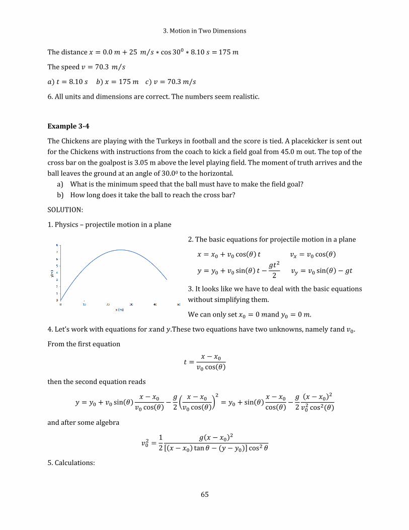
3. Motion in Two Dimensions
65
The distance 𝑥 = 0.0 𝑚 + 25 𝑚 𝑠⁄ ∗ cos 300 ∗ 8.10 𝑠 = 175 𝑚
The speed 𝑣 = 70.3 𝑚 𝑠⁄
𝑎) 𝑡 = 8.10 𝑠 𝑏) 𝑥 = 175 𝑚 𝑐) 𝑣 = 70.3 𝑚/𝑠
6. All units and dimensions are correct. The numbers seem realistic.
Example 3-4
The Chickens are playing with the Turkeys in football and the score is tied. A placekicker is sent out
for the Chickens with instructions from the coach to kick a field goal from 45.0 m out. The top of the
cross bar on the goalpost is 3.05 m above the level playing field. The moment of truth arrives and the
ball leaves the ground at an angle of 30.00 to the horizontal.
a) What is the minimum speed that the ball must have to make the field goal?
b) How long does it take the ball to reach the cross bar?
SOLUTION:
1. Physics – projectile motion in a plane
2. The basic equations for projectile motion in a plane
𝑥 = 𝑥0 + 𝑣0 cos(𝜃) 𝑡 𝑣𝑥 = 𝑣0 cos(𝜃)
𝑦 = 𝑦0 + 𝑣0 sin(𝜃) 𝑡 −𝑔𝑡2
2 𝑣𝑦 = 𝑣0 sin(𝜃) − 𝑔𝑡
3. It looks like we have to deal with the basic equations
without simplifying them.
We can only set 𝑥0 = 0 𝑚and 𝑦0 = 0 𝑚.
4. Let’s work with equations for 𝑥and 𝑦.These two equations have two unknowns, namely 𝑡and 𝑣0.
From the first equation
𝑡 =𝑥 − 𝑥0
𝑣0 cos(𝜃)
then the second equation reads
𝑦 = 𝑦0 + 𝑣0 sin(𝜃)𝑥 − 𝑥0
𝑣0 cos(𝜃)−
𝑔
2(
𝑥 − 𝑥0
𝑣0 cos(𝜃))
2
= 𝑦0 + sin(𝜃)𝑥 − 𝑥0
cos(𝜃)−
𝑔
2
(𝑥 − 𝑥0)2
𝑣02 cos2(𝜃)
and after some algebra
𝑣02 =
1
2
𝑔(𝑥 − 𝑥0)2
[(𝑥 − 𝑥0) tan 𝜃 − (𝑦 − 𝑦0)] cos2 𝜃
5. Calculations:

3.7 Examples
66
𝑣02 = 0.5
9.8 𝑚 𝑠2 ∙ (45.0 𝑚)2⁄
[45 𝑚 ∙ tan 300 − (3.05 𝑚 − 0 𝑚)] cos2 300= 577 𝑚2 𝑠2⁄ 𝑣0 = 24.0 𝑚 𝑠⁄
𝑡 = 2.16 𝑠
6. Looking back: The dimensions and units are correct. The speed (24 m/s or 54 mph) looks
challenging but reasonable. The time seems correct.

3. Motion in Two Dimensions
67
Example 3-5*
Flying in crosswind
The compass of an airplane indicates that it is headed due north, and its airspeed indicator shows that
it is moving through the air at speed 240 km/h. If there is a wind of 100 km/h from west to east,
a) What is the velocity of the airplane relative to the ground?
SOLUTION:
1. Physics – Relative motion in a plane with constant velocities
2. Equations
�⃗�𝑃𝐸 = �⃗�𝑃𝐴 + �⃗�𝐴𝐸
3. and 4. We can find the solution immediately from the equation above
using geometry of vector components. Let’s use vector components as the
most general approach
�⃗�𝑃𝐴 = 0𝑥 + 𝑣𝑃𝐴�̂��⃗�𝐴𝐸 , �⃗�𝐴𝐸 = 𝑣𝐴𝐸𝑥 + 0�̂�,
�⃗�𝑃𝐸 = (0 + 𝑣𝐴𝐸)�̂� + (𝑣𝑃𝐴 + 0)�̂�
𝑣𝑃𝐸 = √(0 + 𝑣𝐴𝐸)2 + (𝑣𝑃𝐴 + 0)2, 𝛼 = arctan 𝑣𝐴𝐸 𝑣𝑃𝐴⁄
Here we use 𝑥 and �̂� as notations for unit vectors in 𝑥- and 𝑦-directions.
5. Calculations
Since we are not asked about specific units of velocity, we may proceed with km/h
𝑣𝑃𝐸 = √(240 𝑘𝑚 ℎ⁄ )2 + (100 𝑘𝑚 ℎ⁄ )2 = 260 𝑘𝑚/ℎ
𝛼 = arctan 𝑣𝐴𝐸 𝑣𝑃𝐴⁄ = arctan 100 240⁄ = 230
6. The dimensions and units look right (it is rather unlikely to make an error with this simple
problem). The numerical results seem reasonable.

3.7 Examples
68
Example 3-6*
Flying in crosswind II
An airspeed indicator shows that an airplane is moving through the air at speed 240 km/h. If there
is a wind of 100 km/h from west to east
a) In what direction should the pilot head to travel due north.
b) What will be his velocity relative to the earth?
SOLUTION:
1. Physics – Relative motion in a plane with constant velocities
2. Equations
�⃗�𝑃𝐸 = �⃗�𝑃𝐴 + �⃗�𝐴𝐸
3. and 4. We can find the solution using vector components. Let’s use vector
components as the most general approach
�⃗�𝑃𝐴 = −𝑣𝑃𝐴 sin 𝛽 𝑥 + 𝑣𝑃𝐴 cos 𝛽 �̂� �⃗�𝐴𝐸 = 𝑣𝐴𝐸�̂� + 0�̂�,
�⃗�𝑃𝐸 = (𝑣𝐴𝐸 − 𝑣𝑃𝐴 sin 𝛽)�̂� + (𝑣𝑃𝐴 cos 𝛽 + 0)�̂�
sin 𝛽 = 𝑣𝐴𝐸/ 𝑣𝑃𝐴
Here we use 𝑥 and �̂� as notations for unit vectors in 𝑥- and 𝑦-directions.
By the way, using equation for the angle 𝛽 iy is easy to show that
𝑣𝑃𝐸 = 𝑣𝑃𝐴 cos 𝛽 = √𝑣𝑃𝐴2 − 𝑣𝐴𝐸
2
5. Calculations
𝑣𝑃𝐸 = √(240 𝑘𝑚 ℎ⁄ )2 − (100 𝑘𝑚 ℎ⁄ )2 = 218 𝑘𝑚/ℎ
𝛽 = arcsin 100 240⁄ = 250
6. The dimensions and units look right (it is rather unlikely to make an error with this simple
problem). The numerical results seem reasonable

4. Newton’s Laws of Motion
69
4 Newton’s Laws of Motion
4.1 Dynamics
Kinematics equations of motion (specifically motion with constant acceleration) are essentially
mathematical equations. The equations do not have any physics or causes of motion.
Dynamics of motion describes motion together with its cause. The discovery of the laws of dynamics,
or the laws of motion, was a dramatic moment in the history of science. Before Sir Isaac Newton's
time (1642 – 1727), the motions of things like the planets were a mystery, but after Newton there was
complete understanding. The motions of objects around us (from a grain of sand to stars and planets),
could all be analyzed completely after Newton's laws were enunciated.
Galileo made a great advance in the understanding of motion when he discovered the principle of
inertia: if an object is left alone, or not disturbed, it continues to move with a constant velocity in a
straight line if it was originally moving, or it continues to stand still if it was just standing still (looks
counterintuitive, isn’t it). It required a certain imagination to find the right rule, and that imagination
was supplied by Galileo.
Of course, the next thing which is needed is a rule for finding how an object changes its speed if
something is affecting it. That is the contribution of Newton. Newton wrote down three laws
(published in 1687): The First Law was a mere restatement of the Galilean principle of inertia just
described. The Second Law gave a specific way of determining how the velocity changes under
different influences called forces. The Third Law is a relationship between the forces that two
interacting bodies exert on each other.

4.2 Force and Interaction
70
Newton’s laws are truly fundamental, for they cannot be deduced or proved from other principles.
Newton’s laws are based on observations made by many scientists before Newton.
Newton’s laws are the foundation of classical mechanics.
There are two situations when Newtonian mechanics cannot be applied, namely if the speed of
interacting bodies is comparable with the speed of light (then we use Einstein’s special theory of
relativity), and if the interacting bodies are comparable with (or smaller than) atomic scale (then we
use quantum mechanics). We can view Newtonian mechanics as a special case of the two above
fundamental theories. However, Newtonian mechanics can be applied to vast majority of situations,
especially on our Human scale.
4.2 Force and Interaction
Although it is interesting and worthwhile to study the physical laws simply because they help us to
understand and to use nature, one ought to stop every once in a while and think, "What do they really
mean?" Well, we can intuitively sense the meaning of force. In physics, the answer is simple: "If a body
is accelerating, then there is a force on it."
Since forces always come in pairs we can also say that a force is an interaction between two bodies or
a body and its environment.
In nature, there are three only fundamental forces (gravity, electroweak force and strong force). All
three forces originate from long-distance interactions at microscopic level.
Since the electromagnetic part of the weak part of the electroweak force act on different scales it is
convenient for multiple applications to consider them as two distinct forces.
Figure 23 Relative strength and the range of interaction of the four fundamental forces.
Many scientists think that all the fundamental forces are the manifestations of a single force which
has yet to be discovered.
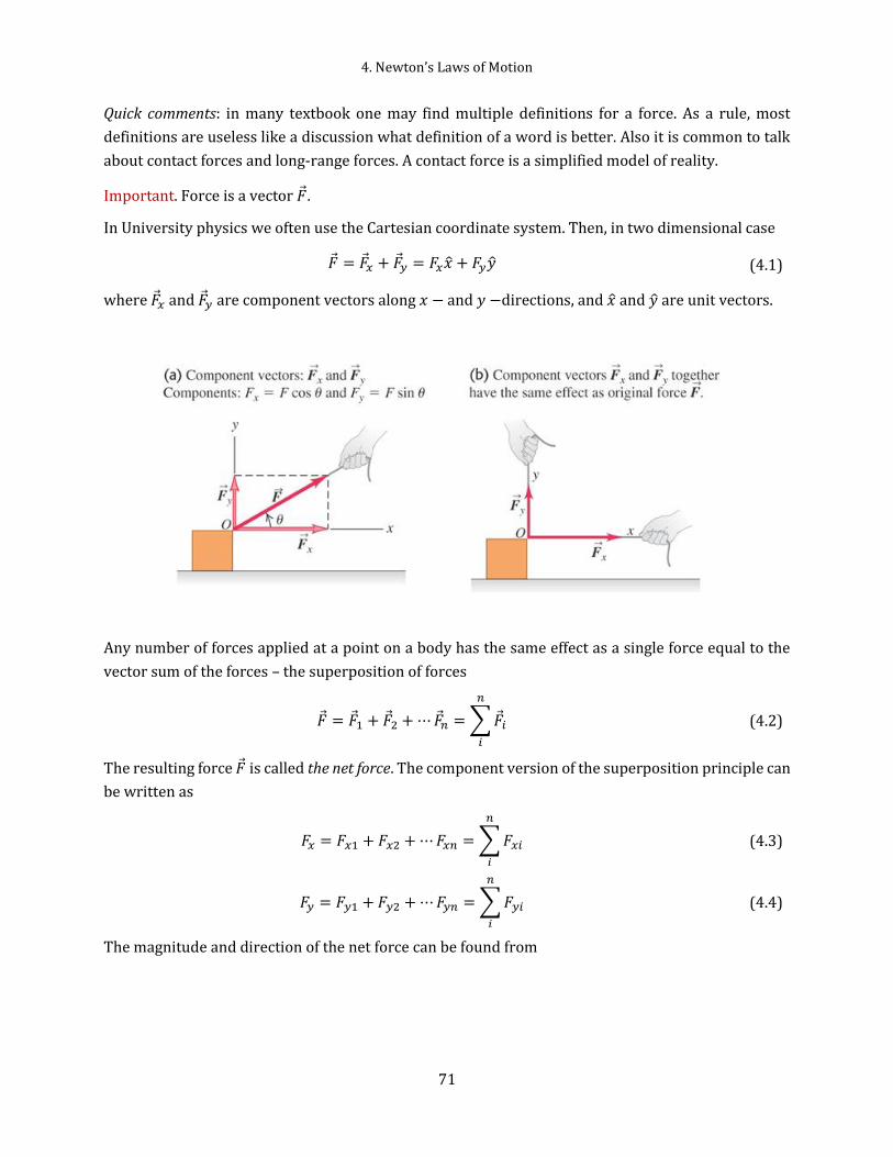
4. Newton’s Laws of Motion
71
Quick comments: in many textbook one may find multiple definitions for a force. As a rule, most
definitions are useless like a discussion what definition of a word is better. Also it is common to talk
about contact forces and long-range forces. A contact force is a simplified model of reality.
Important. Force is a vector �⃗�.
In University physics we often use the Cartesian coordinate system. Then, in two dimensional case
�⃗� = �⃗�𝑥 + �⃗�𝑦 = 𝐹𝑥�̂� + 𝐹𝑦�̂� (4.1)
where �⃗�𝑥 and �⃗�𝑦 are component vectors along 𝑥 − and 𝑦 −directions, and 𝑥 and �̂� are unit vectors.
Any number of forces applied at a point on a body has the same effect as a single force equal to the
vector sum of the forces – the superposition of forces
�⃗� = �⃗�1 + �⃗�2 + ⋯ �⃗�𝑛 = ∑ �⃗�𝑖
𝑛
𝑖
(4.2)
The resulting force �⃗� is called the net force. The component version of the superposition principle can
be written as
𝐹𝑥 = 𝐹𝑥1 + 𝐹𝑥2 + ⋯ 𝐹𝑥𝑛 = ∑ 𝐹𝑥𝑖
𝑛
𝑖
(4.3)
𝐹𝑦 = 𝐹𝑦1 + 𝐹𝑦2 + ⋯ 𝐹𝑦𝑛 = ∑ 𝐹𝑦𝑖
𝑛
𝑖
(4.4)
The magnitude and direction of the net force can be found from

4.2 Force and Interaction
72
𝐹 = √𝐹𝑥2 + 𝐹𝑦
2 , tan 𝜃 = 𝐹𝑦 𝐹𝑥⁄ (4.5)
Forces act independently of each other: neither of them is modified by being applied at the same time
as the other. Superposition works for any number of forces.

4. Newton’s Laws of Motion
73
4.3 Newton’s First Law
Here is an equivalent statement: In the absence of forces, a stationary particle remains stationary and
a moving particle continues to move with unchanging speed in the same direction.
4.3.1 Inertial frames
Newton’s formulation has two important implications:
1. Reference frames that move with constant velocities relative to each other are equivalent.
These are called inertial frames of reference
2. Forces are the same in all inertial frames
State of rest from point-of-view of one observer is a state of constant velocity from point-of-view of
another. It isn’t mere motion that we need to explain – it is the change in state of motion
(acceleration).
If non-zero net force is applied to a particle - all inertial observers see the same effect, viz. force is
parallel to acceleration.
If acceleration is the same in all inertial frames, then force will be the same in all inertial frames
All forces behave in the same way: they all produce accelerations parallel to their directions.
4.4 Newton’s Second Law
�⃗� = 𝑚�⃗� (4.6)
In this equation �⃗� denotes the vector sum of all forces on the particle and �⃗� is the particle’s
acceleration.
�⃗� =𝑑�⃗�
𝑑𝑡=
𝑑2𝑟
𝑑𝑡2
Second Law effectively defines mass: acceleration and force can be measured independently mass is
then determined from Newton’s second law.
Mass in Newton’s second law is a measure of inertia. It is a scalar quantity called inertial mass. Mass
is an inherent property of an object and is independent of the object’s surroundings and of the method
used to measure it.
In the absence of external force, a particle moves with constant velocity �⃗�
For any particle of mass 𝑚, the net force �⃗� on the particle is always
equal to the mass 𝑚 times the particle’s acceleration:

4.4 Newton’s Second Law
74
Mass: The notation: 𝑚, the SI Unit: 𝑘𝑔.
Force: The notation: �⃗�, the SI unit: 𝑛𝑒𝑤𝑡𝑜𝑛. We can use the standard kg to define the SI unit of force
as
1 𝑁 = 1 𝑘𝑔 ∙ 𝑚 𝑠2⁄
Important:
1. Newton’s second law is a vector equation.
In practical applications it is convenient to use it in component form
∑𝐹𝑥 = 𝑚𝑎𝑥
∑𝐹𝑦 = 𝑚𝑎𝑦
2. The statement of Newton’s second law refers to external forces, i.e. forces exerted on the body
by other bodies in its environment
3. The mass 𝑚 in �⃗� = 𝑚�⃗� is constant
4. Newton’s second law is valid only in inertial frames of reference.
Note: Newton formulated his second law in terms of momentum, i.e.
�⃗� =𝑑𝑝
𝑑𝑡 where �⃗� = 𝑚�⃗�
the rate of change of the momentum of a body is directly proportional to the net force acting on it,
and the direction of the change in momentum takes place in the direction of the net force
4.4.1 Mass and Weight
There is a difference to be understood between the weight of an object and its inertia. (How hard it is
to get it going is one thing, and how much it weighs is something else.) Weight and inertia are
proportional, and on the earth's surface are often taken to be numerically equal, which causes certain
confusion. On Mars, weights would be different but the amount of force needed to overcome inertia
would be the same.
We use the term mass as a quantitative measure of inertia, and we may measure mass, for example,
by swinging an object in a circle at a certain speed and measuring how much force we need to keep it
in the circle. In this way we find a certain quantity of mass for every object.
Weight of a body is the force on it by the gravity �⃗�𝑔 = �⃗⃗⃗⃗� = 𝑚�⃗�. Thus, the weight is a vector. Its SI unit
is a newton (in British units the unit of weight is a pound).
When we buy in a grocery store - do we buy mass or weight?
Good to know: On Earth 𝑔 depends on your altitude. On other planets, gravity will likely have an
entirely new value, for example, on the moon 1.62 m/s2, or 0.165*𝑔.
Attention: objects in orbit are not actually weightless; they do have weight since they do experience
the force due to gravity, and are accelerated by it. Their state is correctly described as free-fall, when
objects and everything in their environment is falling under the influence of gravity.

4. Newton’s Laws of Motion
75
Attention: Heavier objects do not fall faster. It is the acceleration that defines how fast (not the force),
namely �⃗� = �⃗�𝑔 𝑚 = 𝑚�⃗� 𝑚⁄ = �⃗�⁄ (the same acceleration for all objects in the absence of air
resistance).
4.5 Newton’s Third Law
A force of interaction on a body is always the result of interaction with another body, so forces always
come in pairs.
or “For every Action, there is an equal but opposite Reaction”.
Note that
1. Both Action and Reaction forces are the same physical origin
2. Action and Reaction act on different objects (�⃗�21 acts on 1, and �⃗�12 acts on 2)
Figure 24 The horse-and-cart dilemma. The horse pulls on the cart, and the cart pulls back with a force of equal magnitude. So, how can the pair ever get moving? The net force on the horse involves forces from different third-laws pairs. Their magnitudes are not equal and the horse experiences a net force in the forward direction.
If object 1 exerts a force �⃗�21 on object 2, then object 2 always exerts
force �⃗�12 on object 1 given by
�⃗�12 = −�⃗�21

4.6 Free body diagrams
76
4.6 Free body diagrams
A free-body diagram is a graphical representation of all the forces acting on an object. Free-body
diagrams are a powerful tool for solving problems. IDEA - replace an actual environment of an object
as a set of forces acting on that object
Free-body diagrams show all forces acting on a particular body.
𝐹 = �⃗�1 + �⃗�2 + ⋯ �⃗�𝑛 = ∑ �⃗�𝑖
𝑛
𝑖
Key ideas for drawing a free-body diagram:
1. Include ALL forces acting on the body matter.
2. When a problem includes more than one body – draw a separate free-body diagram for each
body.
3. Not to include: any forces that the body exerts on any other body.
4. Not to include: non-existing forces (no object – no force).
When constructing a free-body diagram, it is a good idea to choose your coordinate system so that
the motion of an object is along one of the axes.
Attention: So far we consider only translational motion (bodies cannot rotate), when all points of a
body move with the same velocity (in the same direction with the same speed). Rotation of rigid
bodies will be considered in chapters 9 – 11.

4. Newton’s Laws of Motion
77
4.7 Examples
Example 4-1
An advertisement claims that a particular automobile can “stop on a dime”. What net force would
actually be necessary to stop a 1000-kg automobile (about 2,200 lb) travelling at 55 mph in a distance
equal to the diameter of a dime, which is 1.6 cm?
SOLUTION:
1. Physics – Newton’s second law and one dimensional motion with constant acceleration
2. The basic equations
�⃗� = 𝑚�⃗�
𝑥 = 𝑥0 + 𝑣0𝑡 +𝑎𝑡2
2
𝑣 = 𝑣0 + 𝑎𝑡
3. The motion is one dimensional, therefore we can use 𝐹 = 𝑚𝑎, and the final velocity of the car is 𝑣 =
0.
To find the force we need to know the acceleration, which we can find from the kinematic equations
4. From the third equation 𝑡 = −𝑣0/𝑎, then the second equation is
𝑥 = 𝑥0 − 𝑣0 (𝑣0
𝑎) +
1
2𝑎 (
𝑣0
𝑎)
2
2𝑎(𝑥 − 𝑥0) = −2𝑣02 + 𝑣0
2
𝑣02 = −2𝑎(𝑥 − 𝑥0)
The final velocity of the car is 0 m/s, then
𝑎 = −𝑣0
2
2(𝑥 − 𝑥0)
The magnitude of the net force then is
𝐹 = 𝑚𝑣0
2
2(𝑥 − 𝑥0)
5. Calculations
The initial data in SI units (we use 1 mile = 1609 m, 1 m = 100 cm, 1 h = 3600 s)
55 𝑚𝑝ℎ = 55 𝑚𝑖𝑙𝑒
ℎ (
1609 𝑚
1 𝑚𝑖𝑙𝑒) (
1 ℎ
3600 𝑠) = 24.59 𝑚/𝑠
1.6 𝑐𝑚 = 1.6 𝑐𝑚 (1 𝑚
100 𝑐𝑚) = 0.016 𝑚
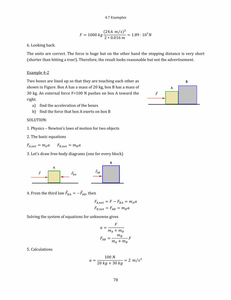
4.7 Examples
78
𝐹 = 1000 𝑘𝑔(24.6 𝑚 𝑠⁄ )2
2 ∗ 0.016 𝑚= 1.89 ∙ 107𝑁
6. Looking back.
The units are correct. The force is huge but on the other hand the stopping distance is very short
(shorter than hitting a tree!). Therefore, the result looks reasonable but not the advertisement.
Example 4-2
Two boxes are lined up so that they are touching each other as
shown in Figure. Box A has a mass of 20 kg, box B has a mass of
30 kg. An external force F=100 N pushes on box A toward the
right.
a) find the acceleration of the boxes
b) find the force that box A exerts on box B
SOLUTION:
1. Physics – Newton’s laws of motion for two objects
2. The basic equations
𝐹𝐴,𝑛𝑒𝑡 = 𝑚𝐴𝑎 𝐹𝐵,𝑛𝑒𝑡 = 𝑚𝐵𝑎
3. Let’s draw free-body diagrams (one for every block)
4. From the third law �⃗�𝐵𝐴 = −�⃗�𝐴𝐵, then
𝐹𝐴,𝑛𝑒𝑡 = 𝐹 − 𝐹𝐵𝐴 = 𝑚𝐴𝑎
𝐹𝐵,𝑛𝑒𝑡 = 𝐹𝐴𝐵 = 𝑚𝐵𝑎
Solving the system of equations for unknowns gives
𝑎 =𝐹
𝑚𝐴 + 𝑚𝐵
𝐹𝐴𝐵 =𝑚𝐵
𝑚𝐴 + 𝑚𝐵𝐹
5. Calculations
𝑎 =100 𝑁
20 𝑘𝑔 + 30 𝑘𝑔= 2 𝑚 𝑠2⁄

4. Newton’s Laws of Motion
79
𝐹𝐴𝐵 =30 𝑘𝑔
20 𝑘𝑔 + 30 𝑘𝑔100 𝑁 = 60 𝑁
6. Looking back
The units are correct. The magnitude of 𝐹𝐴𝐵 itself does not tell much, but we see that 𝐹𝐴𝐵 < 𝐹 as
expected (because the external force �⃗� pushes two boxes and has to be large that the action-reaction
force between the blocks.
Example 4-3
Two masses 𝑚1 and 𝑚2 situated on a frictionless, horizontal surface are connected by a light string.
A force �⃗� is exerted on one of the masses to the right. Determine the acceleration of the system and
the tension T in the string.
SOLUTION:
1. Physics – Newton’s laws of motion for two objects
2. The basic equations
𝐹1,𝑛𝑒𝑡 = 𝑚1𝑎 𝐹2,𝑛𝑒𝑡 = 𝑚2𝑎
3. Let’s draw free-body diagrams (one for every block)
Then for the first block
𝑇 = 𝑚1𝑎
and for the second block
𝐹 − 𝑇 = 𝑚2𝑎
4. Thus we get two equations with two unknowns 𝑇 and 𝑎. The solutions are
𝑎 =𝐹
𝑚1 + 𝑚2, 𝑇 =
𝑚1
𝑚1 + 𝑚2𝐹

4.7 Examples
80
5. Calculations – no numbers, nothing to calculate
6. Looking back
The dimensions are correct. Let’s also note that the solutions are remarkably similar to example 4-2.
Example 4-4
An aerostat of mass 𝑚 starts coming down with a constant acceleration 𝑎. Determine the ballast mass
to be dumped for the aerostat to reach the upward acceleration of the same magnitude. The air drag
is to he neglected.
SOLUTION:
1. Physics – Newton’s laws of motion for one object with two forces
2. The basic equations
𝐹𝑛𝑒𝑡 = 𝑚𝑎
3. Let’s draw free-body diagram
where �⃗�𝑔 = 𝑚�⃗� is the force of gravity and �⃗�𝑢𝑝 is the lifting force. Then when the
aerostat goes down
𝐹𝑢𝑝 − 𝑚𝑔 = −𝑚𝑎
and for goinf up we drop a mass 𝑚′
𝐹𝑢𝑝 − (𝑚 − m′)𝑔 = (𝑚 − 𝑚′)𝑎
4. Thus we have two equations with two unknowns, namely 𝐹𝑢𝑝 and 𝑚′.
From the first equation 𝐹𝑢𝑝 = 𝑚𝑔 − 𝑚𝑎, then the second equation reads
𝑚𝑔 − 𝑚𝑎 − (𝑚 − m′)𝑔 = (𝑚 − 𝑚′)𝑎.
Solving for 𝑚′ gives
𝑚′ = 2𝑚𝑎
𝑔 + 𝑎
5. Calculations (no numbers – no calculations)
6. Looking back
The dimension of the answer [mass] is correct.

5. Applying Newton’s Laws
81
5 Applying Newton’s Laws
5.1 Forces
A true understanding of Newton's laws requires a discussion of specific forces. In this chapter we deal
with following forces
Gravitational force �⃗�𝑔
Normal force �⃗⃗⃗�
Tension �⃗⃗�
Frictional force 𝑓𝜇
Spring force �⃗�𝑠
5.1.1 Gravitational force
A gravitational force on a body is a pull that is directed toward a second body. In this chapter we do
not discuss the nature of this force, and we usually consider that the second body is Earth.
The magnitude:
𝐹𝑔 = 𝑚𝑔 (5.1)
The direction is directly toward the center of Earth (toward the ground)
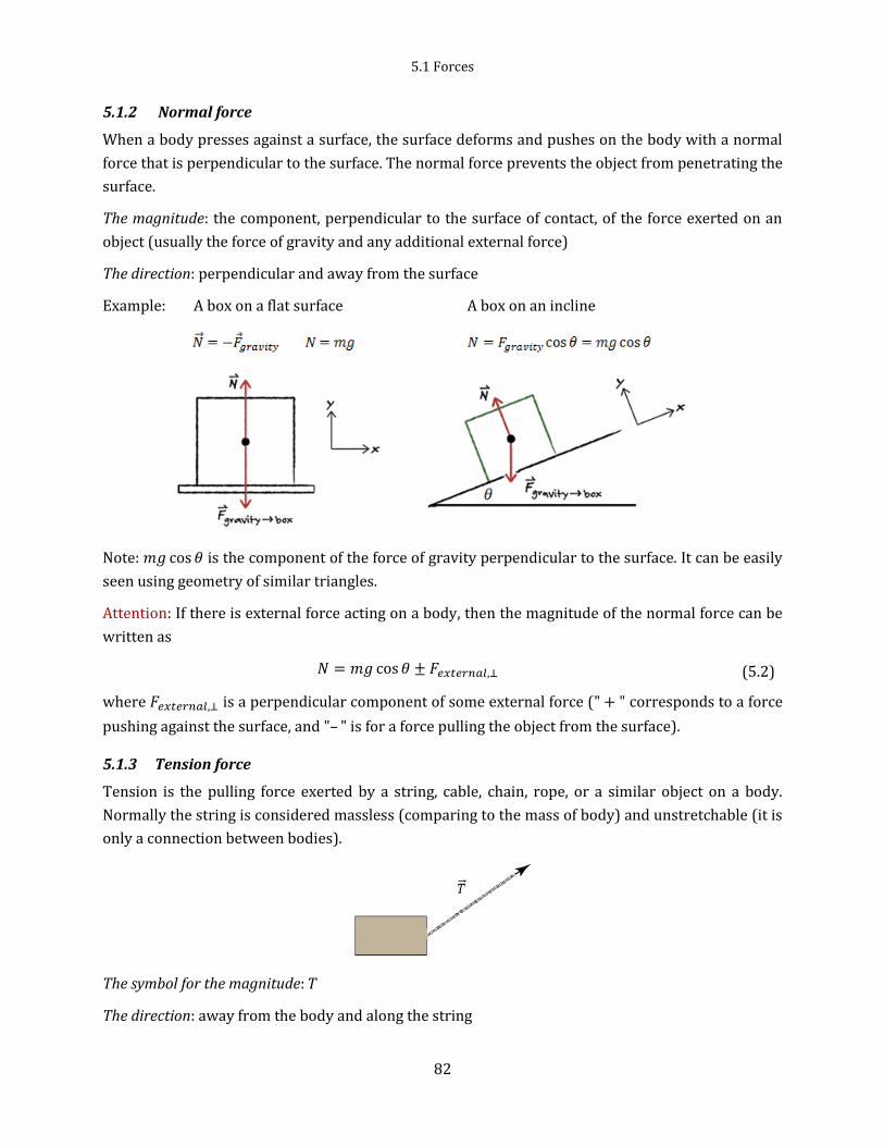
5.1 Forces
82
5.1.2 Normal force
When a body presses against a surface, the surface deforms and pushes on the body with a normal
force that is perpendicular to the surface. The normal force prevents the object from penetrating the
surface.
The magnitude: the component, perpendicular to the surface of contact, of the force exerted on an
object (usually the force of gravity and any additional external force)
The direction: perpendicular and away from the surface
Example: A box on a flat surface A box on an incline
Note: 𝑚𝑔 cos 𝜃 is the component of the force of gravity perpendicular to the surface. It can be easily
seen using geometry of similar triangles.
Attention: If there is external force acting on a body, then the magnitude of the normal force can be
written as
𝑁 = 𝑚𝑔 cos 𝜃 ± 𝐹𝑒𝑥𝑡𝑒𝑟𝑛𝑎𝑙,⊥ (5.2)
where 𝐹𝑒𝑥𝑡𝑒𝑟𝑛𝑎𝑙,⊥ is a perpendicular component of some external force (" + " corresponds to a force
pushing against the surface, and "– " is for a force pulling the object from the surface).
5.1.3 Tension force
Tension is the pulling force exerted by a string, cable, chain, rope, or a similar object on a body.
Normally the string is considered massless (comparing to the mass of body) and unstretchable (it is
only a connection between bodies).
The symbol for the magnitude: 𝑇
The direction: away from the body and along the string

5. Applying Newton’s Laws
83
5.1.4 Frictional force
Microscopically, friction is a very complicated phenomenon.
Macroscopically, at large-scale level, it is relatively simple.
Phenomenologically (empirically), to a fairly good approximation, the frictional force is proportional
to magnitude of normal force, and has a more or less constant coefficient
𝑓 = 𝜇𝑁 (5.3)
where 𝜇 is called the coefficient of friction, and 𝑁 is the normal force. Although this coefficient is not
exactly constant, the formula is a good empirical rule for judging approximately the amount of force
that will be needed in certain practical or engineering circumstances. If the normal force or the speed
of motion gets too big, the law fails because of the excessive heat generated. It is important to realize
that each of these empirical laws has its limitations, beyond which it does not really work.
Static friction (a body does not move):
1. If the body does not move, then the static frictional force 𝑓𝑠 and the component of �⃗� that is
parallel to the surface balance each other.
2. The magnitude of 𝑓𝑠 has a maximum value that is given by 𝑓𝑠,𝑚𝑎𝑥 = 𝜇𝑠𝑁
where 𝜇𝑠 is a coefficient of static friction, and 𝑁 is the magnitude of the normal force on the body from
the surface.
Direction: parallel to the surface, and is directed opposite the component of an external force.
One must overcome (exceed) the force of static friction it in order to initiate motion of the body along
the surface.
Here is a simple way to determine the coefficient of
static friction. Let’s consider an object on an incline.
When block is not moving, friction force compensates
𝑥 −component of gravitational force:
𝑓𝑠 = 𝑚𝑔 sin 𝜃
However by definition 𝑓𝑠 = 𝜇𝑠𝑁 = 𝜇𝑠𝑚𝑔 cos 𝜃 then
𝑚𝑔 sin 𝜃 = 𝜇𝑠𝑚𝑔 cos 𝜃. Let’s 𝜃𝑚𝑎𝑥 is the largest angle
when the block is still not moving, then
𝜇𝑠 = tan 𝜃𝑚𝑎𝑥 (5.4)
Thus, equation (5.4) provides a way to measure a value of static frictional coefficient.
Note that 𝜇𝑠 can be greater than 1.

5.1 Forces
84
Kinetic friction (a sliding body)
If the body begins to slide along the surface, the magnitude of the frictional force rapidly decreases to
a value 𝑓𝑘 given by
𝑓𝑘 = 𝜇𝑘𝑁
where 𝜇𝑘 is the coefficient of kinetic friction. Note that the kinetic friction does not depend on speed.
Direction: always opposite to the direction of velocity
Useful note: Frictional force is independent of the area of contact between the body and the surface.
Approximate coefficients of static and kinetic friction can be found in many textbooks as well as on
the Web.
Overall:
Rolling Friction1
It’s a lot easier to move a loaded filing cabinet across a horizontal floor using a cart with wheels than
to slide it. How much easier? We can define a coefficient of rolling friction which is the horizontal
force needed for constant speed on a flat surface divided by the upward normal force exerted by the
surface, or 𝑓𝑟 = 𝜇𝑟𝑁. Transportation engineers call the tractive resistance. Typical values of are
0.002 to 0.003 for steel wheels on steel rails and 0.01 to 0.02 for rubber tires on concrete. These
values show one reason railroad trains are generally much more fuel efficient than highway trucks.
1 from University Physics by Young and Freedman

5. Applying Newton’s Laws
85
5.1.5 Fluid resistance and terminal speed
A fluid is anything that can flow - generally either a gas or a liquid. A body moving through a fluid
exerts a force on the fluid to push it out of the way. By Newton’s third law, the fluid pushes back on
the body with an equal and opposite force.
The direction of the fluid resistance force acting on a body is always opposite the direction of the
body's velocity relative to the fluid. The magnitude of the fluid resistance force usually increases with
the speed of the body through the fluid. This is very different from the kinetic friction force between
two surfaces in contact, which we can usually regard as independent of speed.
For very low speeds, the magnitude 𝑓 of the fluid resistance force is approximately proportional to the
body's speed 𝑣:
𝑓 = 𝑏𝑣
where 𝑏 is a proportionality constant that depends on the shape and size of the body and the
properties of the fluid.
In motion through air at high speeds (e.g. the speed of a tossed tennis ball or faster), the resisting force
is approximately proportional to 𝑣2 rather than to 𝑣. It is then called air drag or simply drag. The
magnitude of the drag force is related to the relative speed by
𝑓 =1
2𝐶𝜌𝐴𝑣2
where 𝐶 is experimentally determined drag coefficient, 𝜌 is the air density (mass per volume) and 𝐴
is the effective cross-sectional area of the body (the area of a cross section taken perpendicular to the
velocity �⃗�). The drag coefficient 𝐶 (typical values range from 0.4 to 1.0) is not truly a constant for a
given body, because if 𝑣 varies significantly, the value of 𝐶 can vary as well. Here, we ignore such
complications.
When an object falls from rest through air, the drag force 𝑓 is directed upward; its magnitude
gradually increases from zero as the speed of the body increases. This upward force opposes the
downward gravitational force on the body.
𝑓 − 𝑚𝑔 = −𝑚𝑎

5.1 Forces
86
where 𝑚 is the mass of the body. If the body falls enough, 𝑓 eventually equals 𝑚𝑔, this means that 𝑎 =
0 and so the body's speed no longer increases. The body then falls at a constant speed, called the
terminal speed 𝑣𝑡. From
1
2𝐶𝜌𝐴𝑣2 = 𝑚𝑔
follows
𝑣𝑡 = √2𝑚𝑔
𝐶𝜌𝐴
This expression for terminal speed explains why heavy objects in air tend
to fall faster than light objects. Two objects with the same physical size but
different mass (say, a table-tennis ball and a lead ball with the same radius)
have the same value of 𝐴 but different values of 𝑚. The more massive object
has a higher terminal speed and falls faster. The same idea explains why a
sheet of paper falls faster if you first crumple it into a ball; the mass is the
same, but the smaller size makes 𝐴 smaller thus smaller drag force 𝑓 (less
air drag for a given speed) and 𝑣𝑡 larger.
Note: normally in introductory physics classes we do not deal with the drag
force. However, knowing about it is vital for understanding effects of air resistance in everyday life.
5.1.6 Spring Force
When a spring is stretched from its unstressed length by a distance 𝑥, the force it exerts is found
experimentally to be
𝐹𝑠 = −𝑘(𝑥 − 𝑥0) (5.5)
where the positive constant k, called the spring constant, is a measure of the stiffness of the spring,
and 𝑥0 is the equilibrium position (normally counted as 𝑥0 = 0). A negative value of 𝑥 means the
spring has been compressed a distance |𝑥| from its unstressed length. The negative sign means that
when the spring is stretched (or compressed) in one direction, the force it exerts is in the opposite
direction. This relation is known as Hooke’s law. For small displacements, nearly all restoring forces
obey Hooke’s law.
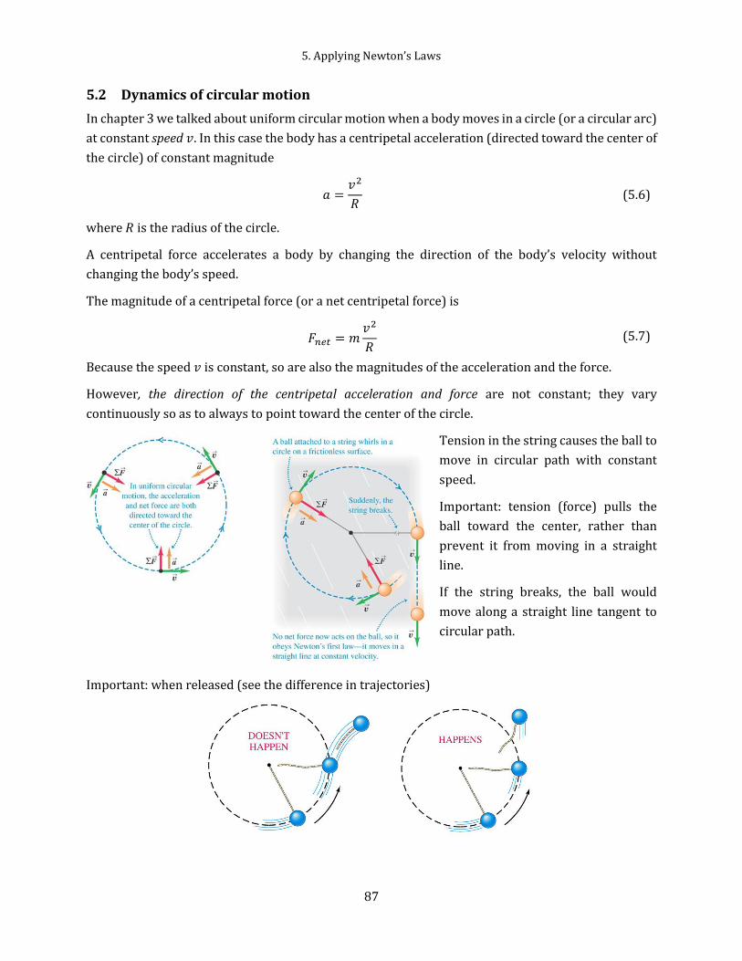
5. Applying Newton’s Laws
87
5.2 Dynamics of circular motion
In chapter 3 we talked about uniform circular motion when a body moves in a circle (or a circular arc)
at constant speed 𝑣. In this case the body has a centripetal acceleration (directed toward the center of
the circle) of constant magnitude
𝑎 =𝑣2
𝑅 (5.6)
where 𝑅 is the radius of the circle.
A centripetal force accelerates a body by changing the direction of the body’s velocity without
changing the body’s speed.
The magnitude of a centripetal force (or a net centripetal force) is
𝐹𝑛𝑒𝑡 = 𝑚𝑣2
𝑅 (5.7)
Because the speed 𝑣 is constant, so are also the magnitudes of the acceleration and the force.
However, the direction of the centripetal acceleration and force are not constant; they vary
continuously so as to always to point toward the center of the circle.
Tension in the string causes the ball to
move in circular path with constant
speed.
Important: tension (force) pulls the
ball toward the center, rather than
prevent it from moving in a straight
line.
If the string breaks, the ball would
move along a straight line tangent to
circular path.
Important: when released (see the difference in trajectories)

5.3 Few guidelines for solving most common problems in “Applying Newton’s Laws”
88
5.3 Few guidelines for solving most common problems in “Applying Newton’s Laws”
As always, it is very productive to follow this procedure for problem solving.
1. Name the type of physics most likely related to the problem in hand. Draw a diagram if needed.
2. Write down the "basic" equations for the physics of the problem.
3. Simplify (when possible) the "basic" equations using given data and conditions.
4. Solve the "adjusted" equation for the unknown(s) using algebra, trigonometry and calculus.
5. Achieve a numerical answer using your symbolic solution and the proper units.
6. Step back, and evaluate your answer in terms of units, dimensions, and most importantly,
common sense.
Since this subject offers so many variations of problems, let elaborate more on most important steps,
namely steps 2 and 3 in the above list.
Many problems on “Applying Newton’s Laws” are either “pure force problems” or a combination “a
force problem” + “a motion with constant acceleration problem”. In the following we are going to
concentrate “force problems”. Here are most important points that may help you to develop a
systematic approach to attacking problems from simple ones to more challenging.
Point 1: Ask yourself a question - How many objects do I need to consider? Normally, in physics 231
we deal with one or two objects (having three or four objects are much less common problems).
Point 2: Draw free-body diagrams. One diagram for every object! You may find it helpful to check
every force from the table below. And if you do have it, then put it on your free-body diagram with a
proper direction.
Summary of forces
Force Magnitude Direction
Gravity 𝐹𝑔 = 𝑚𝑔 toward the ground
Normal 𝑁
= 𝑚𝑔 cos 𝜃 ± 𝐹𝑒𝑥𝑡𝑒𝑟𝑛𝑎𝑙,⊥
perpendicular to the surface (and away)
Tension 𝑇 along the string
Friction (static) 𝑓𝑠,𝑚𝑎𝑥 ≤ 𝜇𝑠𝑁 opposite the component of external force and
parallel to the surface
Friction (kinetic) 𝑓𝑘 = 𝜇𝑘𝑁 always opposite to the direction of velocity
Centripetal force 𝐹𝑐 = 𝑚𝑣2
𝑟 toward the center of rotation
Spring (or elastic) 𝐹𝑠 = −𝑘(𝑥 − 𝑥0) opposite to stretch/compression direction

5. Applying Newton’s Laws
89
Point 3: Choose proper coordinate system for every object. Normally we work with the Cartesian
coordinate system. Choosing wisely helps to reduce algebra and trigonometry load.
For most problems we use the regular orientation (horizontal direction for 𝑥 and vertical one for 𝑦).
However, for incline problems we choose a ‘rotated’ coordinate system
Sure, you may solve incline problems with the regular orientation as well, but then you have much
more trigonometry on your hands.
Point 4: Once we identify all forces and their directions, we write Newton’s second law �⃗�𝑛𝑒𝑡 = 𝑚�⃗� for
every 𝑥 − and 𝑦 − component of every object.
𝐹𝑛𝑒𝑡,𝑥 = ∑𝐹𝑥 = 𝑚𝑎𝑥
𝐹𝑛𝑒𝑡,𝑦 = ∑𝐹𝑦 = 𝑚𝑎𝑦
For objects in equilibrium (that are stationary objects or objects moving with constant velocity) we
apply �⃗� = 0, or �⃗�𝑛𝑒𝑡 = 0. Most problems in Physics I deal with either linear motion or rotational
motion. For uniform rotational motion we write Newton’s second law as
𝐹𝑛𝑒𝑡 = 𝑚𝑣2
𝑟
More explicitly, for linear problems (objects moving along a straight line) we have
4a: One object:
𝐹𝑛𝑒𝑡,𝑥 = 𝑚𝑎𝑥
𝐹𝑛𝑒𝑡,𝑦 = 𝑚𝑎𝑦
4b: Two connected objects (one set of equations for every object).
𝐹𝑛𝑒𝑡1,𝑥 = 𝑚𝑎1𝑥 𝐹𝑛𝑒𝑡2,𝑥 = 𝑚𝑎2𝑥
𝐹𝑛𝑒𝑡1,𝑦 = 𝑚𝑎1𝑦 𝐹𝑛𝑒𝑡2,𝑦 = 𝑚𝑎2𝑦
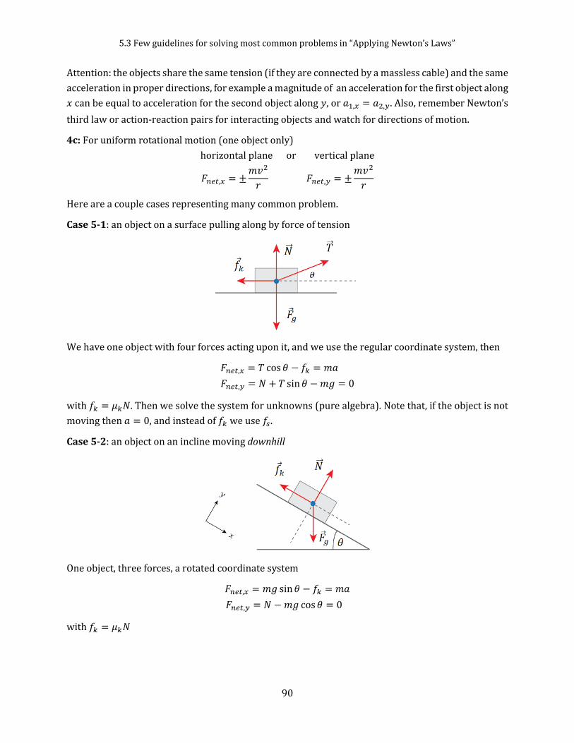
5.3 Few guidelines for solving most common problems in “Applying Newton’s Laws”
90
Attention: the objects share the same tension (if they are connected by a massless cable) and the same
acceleration in proper directions, for example a magnitude of an acceleration for the first object along
𝑥 can be equal to acceleration for the second object along 𝑦, or 𝑎1,𝑥 = 𝑎2,𝑦. Also, remember Newton’s
third law or action-reaction pairs for interacting objects and watch for directions of motion.
4c: For uniform rotational motion (one object only)
horizontal plane or vertical plane
𝐹𝑛𝑒𝑡,𝑥 = ±𝑚𝑣2
𝑟 𝐹𝑛𝑒𝑡,𝑦 = ±
𝑚𝑣2
𝑟
Here are a couple cases representing many common problem.
Case 5-1: an object on a surface pulling along by force of tension
We have one object with four forces acting upon it, and we use the regular coordinate system, then
𝐹𝑛𝑒𝑡,𝑥 = 𝑇 cos 𝜃 − 𝑓𝑘 = 𝑚𝑎
𝐹𝑛𝑒𝑡,𝑦 = 𝑁 + 𝑇 sin 𝜃 − 𝑚𝑔 = 0
with 𝑓𝑘 = 𝜇𝑘𝑁. Then we solve the system for unknowns (pure algebra). Note that, if the object is not
moving then 𝑎 = 0, and instead of 𝑓𝑘 we use 𝑓𝑠.
Case 5-2: an object on an incline moving downhill
One object, three forces, a rotated coordinate system
𝐹𝑛𝑒𝑡,𝑥 = 𝑚𝑔 sin 𝜃 − 𝑓𝑘 = 𝑚𝑎
𝐹𝑛𝑒𝑡,𝑦 = 𝑁 − 𝑚𝑔 cos 𝜃 = 0
with 𝑓𝑘 = 𝜇𝑘𝑁

5. Applying Newton’s Laws
91
Case 5-3: an object attached to two cables (one cable case is way too simple)
There is one object + three forces (gravity and two tensions).
The equations
𝐹𝑛𝑒𝑡,𝑥 = 𝑇2 sin 𝜃2 − 𝑇1 sin 𝜃1 = 0
𝐹𝑛𝑒𝑡,𝑦 = 𝑇1 cos 𝜃1 + 𝑇2 cos 𝜃2 − 𝑚𝑔 = 0
Then we solve for unknowns (normally 𝑇1 and 𝑇2). Note that the angles can be
counted either from vertical (like in the figure) or from horizontal.
Case 5-4: two connected objects (and moving)
Two objects, many forces (four on the first object and
two on the second), regular coordinate system
For the first object
𝐹𝑛𝑒𝑡1,𝑥 = 𝑇 − 𝑓1 = 𝑚1𝑎
𝐹𝑛𝑒𝑡1,𝑦 = 𝑁1 − 𝑚1𝑔 = 0
For the second object
𝐹𝑛𝑒𝑡2,𝑥 = 0
𝐹𝑛𝑒𝑡2,𝑦 = 𝑇 − 𝑚2𝑔 = −𝑚2𝑎
The definition for the frictional force provides one more
equation
𝑓1 = 𝜇1𝑁1
Then we solve the system for unknowns.
If the first body was on incline like on the figure below, then we keep everything the same for the
second object, but we need to do the
following changes for the first one. First
we choose a rotated coordinates for the
first body. Then the equations are
𝐹𝑛𝑒𝑡1,𝑥 = 𝑇 − 𝑓1 − 𝑚1𝑔 sin 𝜃 = 𝑚1𝑎
𝐹𝑛𝑒𝑡1,𝑦 = 𝑁1 − 𝑚1𝑔 cos 𝜃 = 0
with 𝑓1 = 𝜇1𝑁1

5.3 Few guidelines for solving most common problems in “Applying Newton’s Laws”
92
Case 5-5: A ball on a rope that is in circular uniform motion in a horizontal plane, with the rope
making an angle to the horizontal.
One object, two forces, uniform circular motion
Equations
−𝑇 cos 𝜃 = −𝑚𝑣2
𝑟 𝑎𝑙𝑜𝑛𝑔 𝑥
𝑇 sin 𝜃 − 𝑚𝑔 = 0 𝑎𝑙𝑜𝑛𝑔 𝑦

5. Applying Newton’s Laws
93
5.4 Examples
Example 5-1
A passenger of mass 𝑚 stands on a platform scale in an elevator cab.
c) Find a general solution for the scale reading, whatever the vertical motion of the cab
d) What does the scale read is the cab is moving upward at a constant 1.5 m/s2 and 𝑚=80 kg.
1. Physics – 1D (vertical motion), newton’s laws of motion
2. Newton’s second law
�⃗� = 𝑚�⃗�
3. Scales measure weight by reading 𝑁 (weight is directed
down but the normal force is up and perpendicular to the
surface of the scale)
The free-body diagram can be seen on the left
Equation of motion (in 𝑦 −direction 𝐹𝑛𝑒𝑡,𝑦 = 𝑚𝑎𝑦)
𝑁 − 𝑚𝑔 = ±𝑚𝑎
for any choice of acceleration (𝑎 is positive for upward acceleration and negative for downward
acceleration).
4. The equation can be easily solved as
𝑁 = 𝑚(𝑔 ± 𝑎)
5. Calculations for upward motion
𝑁 = 80 𝑘𝑔 ∙ (9.8 + 1.5) 𝑚 𝑠2⁄ = 904 𝑁
Example 5-2
A curious student dangles her cell phone from a thin piece of string while the jetliner she is in takes
off. She notices that the string makes and angle of 250 with respect to the vertical while the aircraft
accelerates for takeoff, which takes about 18 seconds. Estimate the takeoff speed of the aircraft
SOLUTION:
1. Physics – one dimensional motion with constant acceleration and Newton’s second law.
2. For one 1D motion with constant acceleration
𝑥 = 𝑥0 + 𝑣0𝑡 +𝑎𝑡2
2 𝑣 = 𝑣0 + 𝑎𝑡
and Newton’s second law
�⃗� = 𝑚�⃗�

5.4 Examples
94
3. If we knew the acceleration we could estimate the speed from using the kinematic equations.
Free-body diagram for the cell phone
The system of equations
∑𝐹𝑥 = 𝑇 sin 𝜃 = 𝑚𝑎
∑𝐹𝑦 = 𝑇 cos 𝜃 − 𝑚𝑔 = 0
4. The linear system of equations has two unknowns 𝑇 and 𝑎. From the second equation 𝑇 =
𝑚𝑔/ cos 𝜃, then
𝑎 =𝑇 sin 𝜃
𝑚=
𝑚𝑔 sin 𝜃
𝑚 cos 𝜃= 𝑔 tan 𝜃
Using the second kinematic equation we have
𝑣 = 𝑎𝑡 = 𝑔 tan 𝜃 ∙ 𝑡
5. Calculations
𝑣 = 9.8 𝑚 𝑠2⁄ ∙ tan 250 ∙ 18 𝑠 = 82 𝑚 𝑠⁄
6. We have right units for the speed.
The takeoff speed of 82 m/s is about 295 km/h (or 183 mph). It sounds as a realistic speed for a
medium size airplane.
Example 5-3
Suppose you try to move a crate pulling upward on the rope at
an angle 300 above the horizontal. How hard do you have to
pull to keep the crate moving with constant velocity? Is it
easier or harder than puling horizontally? Assume: the crate is
50 kg and the coefficient of kinetic friction is 0.4.

5. Applying Newton’s Laws
95
SOLUTION:
1. Physics – Newton’s laws
2. Newton’s second law (in component form) for motion with constant velocity
∑𝐹𝑥 = 0
∑𝐹𝑦 = 0
3. There is one object with four forces acting upon it: gravity, normal, tension, friction
Let’s draw a free-body diagram for the crate
The system of equations
∑𝐹𝑥 = 𝑇 cos 𝜃 − 𝑓𝑘 = 0
∑𝐹𝑦 = 𝑁 + 𝑇 sin 𝜃 − 𝑚𝑔 = 0
the kinetic frictional force is defined as
𝑓𝑘 = 𝜇𝑘𝑁
4. The linear system with two equations has two unknowns 𝑇 and 𝑁.
The system can easily be solved using substitution. From 2nd equation
𝑁 = 𝑚𝑔 − 𝑇 sin 𝜃
then 𝑓𝑘 = 𝜇𝑘(𝑚𝑔 − 𝑇 sin 𝜃) and from equation for the x-component
𝑇 cos 𝜃 − 𝜇𝑘𝑚𝑔 + 𝜇𝑘𝑇 sin 𝜃 = 0
𝑇(cos 𝜃 + 𝜇𝑘 sin 𝜃) = 𝜇𝑘𝑚𝑔
𝑇 =𝜇𝑘𝑚𝑔
cos 𝜃 + 𝜇𝑘 sin 𝜃
5. Calculations
𝑇 =0.4 ∙ 50𝑘𝑔 ∙ 9.8 𝑚 𝑠2⁄
cos 300 + 0.4 ∙ sin 300= 184 𝑁

5.4 Examples
96
6. The units are correct (newton for the force).
If the angle was 00 then the needed tension would be 196 N. Thus we need less force pulling at some
angle. It is interesting to find what pulling angle would need less force. It happens when cos 𝜃 +
𝜇𝑘 sin 𝜃 takes the largest value
𝑑
𝑑𝜃(cos 𝜃 + 𝜇𝑘 sin 𝜃) = 𝜇𝑘 cos 𝜃 − sin 𝜃 = 0
and tan 𝜃 = 𝜇𝑘. For 𝜇𝑘 = 0.4 the angle is about 220, and the smallest force is 182 N.
Example 5-4
A runaway truck with failed brakes is moving 108 km/h just before the driver steers the truck up the
runaway ramp with an inclination of 300. Assume that the coefficient of friction between the ramp
and the truck is 0.6.
a) What minimum length L must the ramp have to stop along it?
b) How long (in seconds) does it take for the truck to stop?
c) Does the minimum length L increase, decrease, or remain the same for a small passenger car?
SOLUTION
1. Physics – 1D motions with constant acceleration along the ramp, Newton’s second law
2. For one 1D motion with constant acceleration
𝑥 = 𝑥0 + 𝑣0𝑡 +𝑎𝑡2
2 𝑣 = 𝑣0 + 𝑎𝑡
and Newton’s second law
�⃗� = 𝑚�⃗�
3. First we need to find the deceleration of the truck on the ramp. Then we can solve the kinematic
problem to find the stopping distance and time.
The free-body diagram includes all three forces acting
on the truck (gravity, normal, and friction). We choose
the coordinate system as a rotated one with the x-
coordinate parallel to the ramp.
The system of equations
∑𝐹𝑥 = −𝑚𝑔 sin 𝜃 − 𝑓𝑘 = 𝑚𝑎
∑𝐹𝑦 = 𝑁 − 𝑚𝑔 cos 𝜃 = 0
The kinetic frictional force is defined as
𝑓𝑘 = 𝜇𝑘𝑁

5. Applying Newton’s Laws
97
4. The linear system of equations has two unknowns (acceleration and normal force). Solving the
system of equation for the acceleration gives (note: from simple geometry follows that the black 𝜃 is
equal to the green 𝜃 angle)
𝑁 = 𝑚𝑔 cos 𝜃
−𝑚𝑔 sin 𝜃 − 𝜇𝑘𝑚𝑔 cos 𝜃 = 𝑚𝑎
𝑎 = −𝑔(sin 𝜃 + 𝜇𝑘 cos 𝜃)
Now we can work with the kinematic equations. Note that 𝑎 is the deceleration and the kinetic
equations
𝑥 = 𝑥0 + 𝑣0𝑡 +𝑎𝑡2
2 𝑣 = 𝑣0 − 𝑎𝑡
Since the final velocity of the truck is zero at the end of the ramp, then we can easily find the stopping
time and then the distance
𝑡 = −𝑣0
𝑎, 𝑥 = −𝑣0
𝑣0
𝑎+
𝑎
2
𝑣02
𝑎2= −
𝑣02
2𝑎
𝑥 =𝑣0
2
2𝑔(sin 𝜃 + 𝜇𝑘 cos 𝜃)
5. Calculations
In SI units
108 𝑘𝑚 ℎ⁄ = 108 𝑘𝑚
ℎ (
1000 𝑚
1 𝑘𝑚) (
1 ℎ
3600 𝑠) = 30 𝑚/𝑠
𝑎 = 9.8 𝑚 𝑠2⁄ ∙ (sin 300 + 0.6 ∙ cos 300) = 10 𝑚 𝑠2⁄
𝑡 =30 𝑚 𝑠⁄
10 𝑚 𝑠2⁄= 3 𝑠 𝑥 =
(30 𝑚 𝑠⁄ )2
2 ∙ 10 𝑚 𝑠2⁄= 45 𝑚
6. Proper units for the time and distance. Both the time and distance look realistic.
What if the truck was going downhill? How does friction affect the stopping distance? In this case the
direction of the frictional force is in the opposite and then
∑𝐹𝑥 = 𝑚𝑔 sin 𝜃 − 𝑓𝑘 = 𝑚𝑎
∑𝐹𝑦 = 𝑁 − 𝑚𝑔 cos 𝜃 = 0
𝑚𝑔 sin 𝜃 − 𝜇𝑘𝑚𝑔 cos 𝜃 = 𝑚𝑎
𝑎 = 𝑔(sin 𝜃 − 𝜇𝑘 cos 𝜃)
finally
𝑥 =𝑣0
2
2𝑔(𝜇𝑘 cos 𝜃 − sin 𝜃)
The truck cannot stop if 𝜇𝑘 cos 𝜃 − sin 𝜃 ≤ 0.

5.4 Examples
98
Example 5-5
A 12.0-kg box (𝑚1) is connected to an empty 2.00-kg bucket (𝑚2) by
a cord running over a very light frictionless pulley. There is no
appreciable friction on the box, since somebody spilled oil on the
table. The box starts from rest.
a) Find the acceleration of the box and the bucket.
b) What is the tension in the cord?
SOLUTION:
1. Physics: Newton’s laws for two connected objects.
2. Second Newton’s law for 2D case
∑𝐹𝑥 = 𝑚𝑎𝑥 , ∑𝐹𝑦 = 𝑚𝑎𝑦
3. We have two connected objects; therefore we have to write the second law for every object.
Let’s start with free-body diagrams
The system of equations for two objects
𝑇 = 𝑚1𝑎 𝑚1𝑎𝑙𝑜𝑛𝑔 𝑥
𝑁1 − 𝑚1𝑔 = 0 𝑚1 𝑎𝑙𝑜𝑛𝑔 𝑦
𝑇 − 𝑚2𝑔 = −𝑚2𝑎 𝑚2 𝑎𝑙𝑜𝑛𝑔 𝑦
4. Note that according to Newton’s third law the tension in the
cable in the same for both objects (if the cable does not have
mass). The linear system of three equations has three
unknowns. Solving by substitution gives
𝑎 =𝑚2
𝑚2 + 𝑚1𝑔 𝑇 =
𝑚2𝑚1
𝑚2 + 𝑚1𝑔
5. Calculations
𝑎 =2 𝑘𝑔
2 𝑘𝑔 + 12 𝑘𝑔9.8 𝑚 𝑠2⁄ = 1.4 𝑚 𝑠2⁄ , 𝑇 = 12 𝑘𝑔 ∙ 1.4 𝑚 𝑠2⁄ = 16.8 𝑁
6. Looking back
We have proper units for the acceleration and tension. The numbers do not tell much if we can trust
the results, but we may consider an extreme case when 𝑚1 = 0, then 𝑎 = 9.8 𝑚 𝑠2⁄ 𝑇 = 0 𝑁.
Correct. If 𝑚2 = 0, then 𝑎 = 0 also correct.
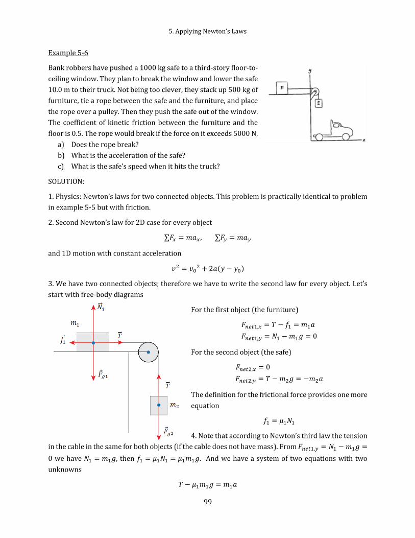
5. Applying Newton’s Laws
99
Example 5-6
Bank robbers have pushed a 1000 kg safe to a third-story floor-to-
ceiling window. They plan to break the window and lower the safe
10.0 m to their truck. Not being too clever, they stack up 500 kg of
furniture, tie a rope between the safe and the furniture, and place
the rope over a pulley. Then they push the safe out of the window.
The coefficient of kinetic friction between the furniture and the
floor is 0.5. The rope would break if the force on it exceeds 5000 N.
a) Does the rope break?
b) What is the acceleration of the safe?
c) What is the safe’s speed when it hits the truck?
SOLUTION:
1. Physics: Newton’s laws for two connected objects. This problem is practically identical to problem
in example 5-5 but with friction.
2. Second Newton’s law for 2D case for every object
∑𝐹𝑥 = 𝑚𝑎𝑥 , ∑𝐹𝑦 = 𝑚𝑎𝑦
and 1D motion with constant acceleration
𝑣2 = 𝑣02 + 2𝑎(𝑦 − 𝑦0)
3. We have two connected objects; therefore we have to write the second law for every object. Let’s
start with free-body diagrams
For the first object (the furniture)
𝐹𝑛𝑒𝑡1,𝑥 = 𝑇 − 𝑓1 = 𝑚1𝑎
𝐹𝑛𝑒𝑡1,𝑦 = 𝑁1 − 𝑚1𝑔 = 0
For the second object (the safe)
𝐹𝑛𝑒𝑡2,𝑥 = 0
𝐹𝑛𝑒𝑡2,𝑦 = 𝑇 − 𝑚2𝑔 = −𝑚2𝑎
The definition for the frictional force provides one more
equation
𝑓1 = 𝜇1𝑁1
4. Note that according to Newton’s third law the tension
in the cable in the same for both objects (if the cable does not have mass). From 𝐹𝑛𝑒𝑡1,𝑦 = 𝑁1 − 𝑚1𝑔 =
0 we have 𝑁1 = 𝑚1𝑔, then 𝑓1 = 𝜇1𝑁1 = 𝜇1𝑚1𝑔. And we have a system of two equations with two
unknowns
𝑇 − 𝜇1𝑚1𝑔 = 𝑚1𝑎

5.4 Examples
100
𝑇 − 𝑚2𝑔 = −𝑚2𝑎
Solving by substitution gives
𝑎 =𝑚2 − 𝜇1𝑚1
𝑚2 + 𝑚1𝑔 𝑇 =
𝑚2𝑚1
𝑚2 + 𝑚1
(1 + 𝜇1)𝑔
The speed can be found from
𝑣2 = 𝑣02 + 2𝑎(𝑦 − 𝑦0)
where we use 𝑎 from equation above if the rope does not break, or 𝑎 = 𝑔 = 9.8 𝑚/𝑠2 if the rope
breaks.
5. Calculations
𝑇 = 4900 𝑁, 𝑎 = 4.9 𝑚/𝑠2
Thus, the rope does NOT break. The safe’s speed at the end is
𝑣 = 9.9 𝑚/𝑠2
6. Looking back
We have proper units for the acceleration and tension. In the absence of friction (𝜇1 = 0) our
equations for the acceleration and tensions are identical to equations from example 5-5.

5. Applying Newton’s Laws
101
Example 5-7
Two masses 𝑚1 and 𝑚2 are connected by a light string that passes over a
frictionless pulley, as in Figure.
Determine
a) the tension in the string,
b) the acceleration of each object,
c) the force that the ceiling exerts on the hook
SOLUTION:
1. Physics: Newton’s laws for two connected objects. (Atwood machine)
2. Second Newton’s law for 2D case for every object
3. We have two connected objects; therefore we have to write the second
law for every object.
Let’s start with free-body diagrams.
This is a system of equations for two objects. Note, for every object we have
only one coordinate, namely 𝑦- component
𝑇 − 𝑚1𝑔 = 𝑚1𝑎
𝑇 − 𝑚2𝑔 = −𝑚2𝑎
4. Note that according to Newton’s third law the tension in the cable in the same for both objects (if
the cable does not have mass).
Attention, we should be careful with signs for the acceleration in both equations. We do not know
what mass is large, and in what direction the masses will move. Thus we assume that the first mass
moves upward (positive acceleration), and the second mass moves downward (negative). Actually it
is not important; a proper sign for acceleration 𝑎 will be derived automatically by solving the system
above.
From the first equation 𝑇 = 𝑚1𝑔 + 𝑚1𝑎, substituting it into the second equation gives
𝑚1𝑔 + 𝑚1𝑎 − 𝑚2𝑔 = −𝑚2𝑎, then (𝑚1 + 𝑚2)𝑎 = (𝑚2 − 𝑚1)𝑔
𝑎 =𝑚2 − 𝑚1
𝑚2 + 𝑚1𝑔
and the tension (after simple algebra) is
𝑇 =2𝑚1𝑚2
𝑚1 + 𝑚2𝑔
The force on the hook can be found from the free-body diagram on the right.
𝑇0 − 𝑇 − 𝑇 = 0, 𝑇0 = 2𝑇 =4𝑚1𝑚2
𝑚1 + 𝑚2𝑔

5.4 Examples
102
6. Looking back
Let’s see what we get if 𝑚1 = 𝑚2 = 𝑚. In this case we get 𝑎 = 0, 𝑇 = 𝑚𝑔 and 𝑇0 = 2𝑚𝑔 as we would
expect for this balanced case.
For 𝑚2 ≫ 𝑚1 he have 𝑎 ≈ 𝑔, (a freely falling body) and 𝑇 ≈ 2𝑚1𝑔.
Example 5-8
A 50-kg refrigerator is placed on the flat floor of a truck. The coefficients of friction between the
refrigerator and floor are s=0.24 and k=0.21. The truck starts to move with an acceleration of
2.5 m/s2. If the refrigerator is 2.0 m from the rear of the truck when the truck starts, how much time
elapses before the refrigerator falls off the truck? How far does the truck travel in this time?
SOLUTION
1. Physics – Newton’s laws, 1D motion with constant acceleration
2. Equations
∑𝐹𝑥 = 𝑚𝑎𝑥 , 𝑓𝑠 = 𝜇𝑠𝑁, 𝑓𝑘 = 𝜇𝑘𝑁
𝑥 = 𝑥0 + 𝑣0𝑡 +𝑎𝑡2
2
𝑣 = 𝑣0 + 𝑎𝑡
3. First we work with the forces acting on the refrigerator.
Assume that the truck moves to the right. Then it is the frictional force that
provides acceleration for the refrigerator! The most acceleration we can get is
𝑎𝑠 = 𝑓𝑠/𝑚. Since 𝑁 = 𝑚𝑔, then 𝑎𝑠 = 𝜇𝑠𝑔. However, as soon as the truck starts
moving with acceleration larger than 𝑎𝑠, the refrigerator starts sliding on the
truck’s bed. Now we deal with kinetic friction, that is equal to 𝑎𝑘 = 𝜇𝑘𝑔. Now,
the truck moves with 𝑎 acceleration but the refrigerator has 𝑎𝑘 < 𝑎
acceleration, or the truck moves faster than the refrigerator with acceleration
𝑎𝑟𝑒𝑙 = 𝑎 − 𝑎𝑘 = 𝑎 − 𝜇𝑘𝑔 . Having this acceleration we can find how much time it will take for the
refrigerator to move along the truck’s bed. From 1D motion with constant acceleration
𝑥 = 𝑥0 + 𝑣0𝑡 +𝑎𝑡2
2, 𝑣0 = 0, 𝑥 − 𝑥0 = 𝑥𝑏𝑒𝑑 =
𝑎𝑟𝑒𝑙𝑡2
2, 𝑡 = √2
𝑥𝑏𝑒𝑑
𝑎𝑟𝑒𝑙= √2
𝑥𝑏𝑒𝑑
𝑎 − 𝜇𝑘𝑔
During this time the truck will move
𝑥𝑡𝑟𝑢𝑐𝑘 =𝑎𝑡2
2= 𝑎
1
22
𝑥𝑏𝑒𝑑
𝑎 − 𝜇𝑘𝑔 =
𝑎
𝑎 − 𝜇𝑘𝑔 𝑥𝑏𝑒𝑑
5. Calculations
𝑡 = 3.0 𝑠, 𝑥𝑡𝑟𝑢𝑐𝑘 = 11 𝑚

5. Applying Newton’s Laws
103
6. Looking back.
The dimensions are correct and the numbers looks sensible.
Note that this problem has very little work with equations, but careful thinking is needed.
Example 5-9
In a loop-the-loop stunt a stuntman is riding a bicycle. Assuming that
the loop is the circle with radius R=2.7 m, what is the least speed the
stuntman has to have at the top of the loop to remain in contact with
it there.
SOLUTION
1. Physics – circular motion and Newton’s laws
2. Equation of motion
𝐹𝑛𝑒𝑡 = 𝑚𝑎 =𝑚𝑣2
𝑅
3. A free-body diagram with all forces
Then
−𝑁 − 𝑚𝑔 = 𝑚(−𝑎)
4. This becomes
−𝑁 − 𝑚𝑔 = 𝑚 (−𝑣2
𝑅)
If the stuntman has the least speed to remain in contact, then he
is on the verge of losing contact with the loop (falling away from
the loop), which means 𝑁 = 0. Thus
−𝑚𝑔 = 𝑚 (−𝑣2
𝑅) and 𝑣 = √𝑔𝑅
Note that this speed requirement is independent of the mass of the stuntman and his bicycle.
5. Calculations
𝑣 = √𝑔𝑅 = √9.8 𝑚 𝑠2⁄ ∙ 2.7 𝑚 = 5.1 𝑚 𝑠⁄
6. Units - correct. We do not have experience with this stunt, but 5.1 m/s (or 11.4 mph) is a reasonable
speed for a bike.
Example 5-10

5.4 Examples
104
A stuntman drives a car at constant speed as he travels through the hill and valley. The cross sections
of both the hill and valley parts can be approximated
by a circle of radius 160 m. The mass of the car is 1000
kg, and the mass of the driver is 80 kg.
a) What is the greatest speed (in mph units) at
which he can drive without the car leaving the road at the top of the hill (point A)?
b) What is the magnitude of the force on the stuntman (in unit of his weight) at the bottom of the hill
(point C)? (note that his speed at point C is the same as at point A).
SOLUTION
1. Physics – circular motion and Newton’s laws
2. Equation of motion
𝐹𝑛𝑒𝑡 = 𝑚𝑎 =𝑚𝑣2
𝑅
3 and 4. A free-body diagram at points A and B is quite simple.
At point A the direction of centripetal acceleration is down, then
𝑁 − 𝑚𝑔 = −𝑚𝑣2
𝑅, and 𝑁 = 𝑚𝑔 −
𝑚𝑣2
𝑅
Losing contact with the road means 𝑁 = 0, then the maximum speed at point A is
𝑣𝑚𝑎𝑥 = √𝑔𝑅
At point B the direction of the centripetal acceleration is up (toward the center of the circle)
𝑁 − 𝑚𝑔 =𝑚𝑣2
𝑅, and 𝑁 = 𝑚𝑔 +
𝑚𝑣2
𝑅
or in units of his weight it will be (keeping in mind that 𝑣 = 𝑣𝑚𝑎𝑥)
and 𝑁𝑤 =𝑁
𝑚𝑔= 1 +
𝑣2
𝑔𝑅= 1 +
𝑔𝑅
𝑔𝑅= 1 + 1 = 2
5. Calculations
𝑣𝑚𝑎𝑥 = √𝑔𝑅 = √9.8 𝑚 𝑠2⁄ ∙ 160 𝑚 = 39.6 𝑚 𝑠⁄ = 89 𝑚𝑝ℎ
𝑁𝑤 = 2
6. Units - correct. The numbers look reasonable.
Example 5-11*

5. Applying Newton’s Laws
105
A 1000-kg car rounds a curve on a road of radius 50 meters. The coefficient of friction between the
pavement and the car is 𝜇𝑠 = 0.60. What is the maximum possible speed to make the turn without
skidding?
a) On a flat road with the coefficient of static friction 𝜇𝑠 = 0.60
b) On a banked icy road with 𝛽 = 100 and 𝜇𝑠 = 0.0
c) On a banked road with 𝛽 = 100 and 𝜇𝑠 = 0.60
SOLUTION:
1. Physics – Uniform circular motion with the following forces: gravity, normal, friction
2. The principal equations are
𝐹𝑛𝑒𝑡,𝑥 = 𝑚𝑣2 𝑟⁄ 𝑓𝑠 = 𝜇𝑠𝑛
however, the net forces are different for various cases. It is clear that the last case (case c) is the most
general, and a) and b) solutions are just special cases
3. For better understanding let’s solve a) then b) and then c)
4a) a flat road
𝐹𝑛𝑒𝑡,𝑥 = 𝑓𝑠 = 𝑚𝑣2
𝑅
𝐹𝑛𝑒𝑡,𝑦 = 𝑛 − 𝑚𝑔 = 0
from the second equation
𝑛 = 𝑚𝑔
then 𝑓𝑠 = 𝜇𝑠𝑛 = 𝜇𝑠𝑚𝑔 and
𝜇𝑠𝑚𝑔 = 𝑚𝑣2
𝑅
𝑎) 𝑣𝑚𝑎𝑥 = √𝜇𝑠𝑔𝑅
4b) a banked icy road
𝐹𝑛𝑒𝑡,𝑥 = 𝑛 sin 𝛽 = 𝑚𝑣2
𝑅
𝐹𝑛𝑒𝑡,𝑦 = 𝑛 cos 𝛽 − 𝑚𝑔 = 0
from the second equation 𝑛 =𝑚𝑔
cos 𝛽 and
𝑚𝑔
cos 𝛽sin 𝛽 = 𝑚
𝑣2
𝑅

5.4 Examples
106
𝑏) 𝑣𝑚𝑎𝑥 = √𝑔𝑅 tan 𝛽
4c) a banked road
Note that we use immediately that 𝑓𝑠 = 𝜇𝑠𝑛
for x-component
𝐹𝑛𝑒𝑡,𝑥 = 𝑛 sin 𝛽 + 𝜇𝑠𝑛 cos 𝛽 = 𝑚𝑣2
𝑅
for y-component
𝐹𝑛𝑒𝑡,𝑦 = 𝑛 cos 𝛽 − 𝜇𝑠𝑛 sin 𝛽 − 𝑚𝑔 = 0
from the second equation
𝑛 =𝑚𝑔
cos 𝛽 − 𝜇𝑠 sin 𝛽
the first equation reads
𝑛(sin 𝛽 + 𝜇𝑠 cos 𝛽) = 𝑚𝑣2
𝑅
and now
𝑚𝑔
cos 𝛽 − 𝜇𝑠 sin 𝛽(sin 𝛽 + 𝜇𝑠 cos 𝛽) = 𝑚
𝑣2
𝑅
𝑐) 𝑣𝑚𝑎𝑥 = √𝑔𝑅(sin 𝛽 + 𝜇𝑠 cos 𝛽)
(cos 𝛽 − 𝜇𝑠 sin 𝛽)
Let’s do a quick check if we can get answers a) and b) from the last equations
If 𝛽 = 0 (flat road) then
𝑣𝑚𝑎𝑥 = √𝑔𝑅(sin 𝛽 + 𝜇𝑠 cos 𝛽)
(cos 𝛽 − 𝜇𝑠 sin 𝛽)= √𝑔𝑅
𝜇𝑠 cos 𝛽
cos 𝛽= √𝜇𝑠𝑔𝑅
If 𝜇𝑠 = 0 (no friction) then
𝑣𝑚𝑎𝑥 = √𝑔𝑅(sin 𝛽 + 𝜇𝑠 cos 𝛽)
(cos 𝛽 − 𝜇𝑠 sin 𝛽)= √𝑔𝑅
sin 𝛽
cos 𝛽= √𝑔𝑅 tan 𝛽
We do get special cases from our general solution c)
5. Calculations

5. Applying Newton’s Laws
107
𝑎) 𝑣𝑚𝑎𝑥 = √𝜇𝑠𝑔𝑅 = 17 𝑚/𝑠
𝑏) 𝑣𝑚𝑎𝑥 = √𝑔𝑅 tan 𝛽 = 9.3 𝑚/𝑠
𝑐) 𝑣𝑚𝑎𝑥 = √𝑔𝑅(sin 𝛽 + 𝜇𝑠 cos 𝛽)
(cos 𝛽 − 𝜇𝑠 sin 𝛽)= 20 𝑚/𝑠
6. How can we validate the numerical answers? Let’s compare the max speeds with our experiences.
In mph units 𝑣𝑎 = 38 𝑚𝑝ℎ 𝑣𝑏 = 21 𝑚𝑝ℎ 𝑣𝑐 = 46 𝑚𝑝ℎ. These speeds look realistic. Besides we can
see that a banked road (case c) provides a bit higher max speed comparing to a flat road (case a).
It is interesting how these max speeds would change on an icy road with 𝜇𝑠 = 0.1. In this case we have
𝑣𝑎 = 16 𝑚𝑝ℎ 𝑣𝑏 = 21 𝑚𝑝ℎ 𝑣𝑐 = 26 𝑚𝑝ℎ

6.1 Energy
108
6 Kinetic Energy, Work, Power
6.1 Energy
Newton’s laws of motion give us a tool to analyze and predict varieties of motion. However, the
analysis is often complicated. We may need to solve numerically a set of differential equations based
on Newton’s laws. Or finding a solution may require details that we do not know.
There is another, very powerful, technique for analyzing motion based on conservation of energy. We
often use this technique when we are not interested in some details but care about only initial and
final states or configurations. On the other hand, energy comes in many different forms. Therefore,
using conservation of energy can be a delicate issue, even for relatively simple systems.
Even though we extensively use the word energy in everyday life, there is no precise definition for it.
Richard Feynman (Nobel Prize in physics) wrote “In physics today, we have no knowledge of what
energy is. We know how to calculate its value for a great variety of situations, but beyond that it’s just
an abstract thing which has only one really important property – conservation”.
6.2 Kinetic Energy
Let’s start our consideration with kinetic energy, namely energy associated with the state of motion
of an object. For an object of mass m travelling with speed v we define kinetic energy as
𝐾 =1
2𝑚𝑣2 (𝑘𝑖𝑛𝑒𝑡𝑖𝑐 𝑒𝑛𝑒𝑟𝑔𝑦)
Energy is a scalar quantity (a number) that is associated with a state (or condition) of one or more
objects.

6. Kinetic Energy, Work, Power
109
The SI unit of kinetic energy as well as any other type of energy is the joule (J)
1 joule = 1 J = 1 kg m2 /s2.
Let’s find out a change in kinetic energy for a particle travelling with constant acceleration along x-
coordinate
𝐾𝑓 − 𝐾𝑖 =1
2𝑚𝑣𝑓
2 −1
2𝑚𝑣𝑖
2 =1
2𝑚(𝑣𝑓
2 − 𝑣𝑖2)
Using 𝑣𝑓2 = 𝑣𝑖
2 + 2𝑎(𝑥𝑓 − 𝑥𝑖) from chapter 2 we can rewrite
𝐾𝑓 − 𝐾𝑖 =1
2𝑚2𝑎(𝑥𝑓 − 𝑥𝑖) = 𝑚𝑎(𝑥𝑓 − 𝑥𝑖) = 𝐹(𝑥𝑓 − 𝑥𝑖)
Thus we have a connection between the change in kinetic energy and a force causing this change.
It is interesting to consider a more general case, namely a motion with a variable force in two or three
dimensions. However, before doing that we need to step back and consider a scalar product of two
vectors.
6.3 Scalar (dot) product of vectors
There are two kinds of product of a vectors but none of them is like a common algebraic
multiplication. The first kind is called the scalar (or dot) product. It produces a result that is a scalar
quantity. The second kind is called the vector (or cross) product. It yields a new vector.
The scalar product of the vectors �⃗� and �⃗⃗� is written as �⃗� ∙ �⃗⃗� and defined to be
�⃗� ∙ �⃗⃗� = 𝑎𝑏 cos 𝜃 (6.1)
here 𝑎 is the magnitude of �⃗�, 𝑏 is the magnitude of �⃗⃗�, and 𝜃 is the angle between the directions of �⃗�
and �⃗⃗�. There are actually two such angles: 𝜃 and 360 − 𝜃. Either can be used because their cosines are
the same.
The scalar product can be rewritten as
�⃗� ∙ �⃗⃗� = 𝑎𝑏 cos 𝜃 = (𝑎 cos 𝜃)𝑏 = 𝑎(𝑏 cos 𝜃)

6.4 Kinetic energy and work
110
The commutative law applies to a scalar product, so we can write
�⃗� ∙ �⃗⃗� = �⃗⃗� ∙ �⃗�
The scalar product involving unit vectors 𝑥 and �̂� (here we use 𝑥
and �̂� for unit vectors notations instead of 𝑖 ̂and 𝑗̂.)
𝑥 ∙ 𝑥 = �̂� ∙ �̂� = (1)(1) cos 0 = 1
𝑥 ∙ �̂� = �̂� ∙ 𝑥 = (1)(1) cos 90 = 0
Then a scalar product of a unit vector 𝑥 and a vector �̂�
𝑥 ∙ �⃗� = 𝑥 ∙ (𝑎𝑥�̂� + 𝑎𝑦�̂�) = 𝑎𝑥�̂� ∙ 𝑥 + 𝑎𝑦𝑥 ∙ �̂� = 𝑎𝑥
gives a projection 𝑎𝑥 of �⃗� onto this unit vector 𝑥.
Let’s calculate a scalar product of two vectors �⃗� and �⃗⃗� using vector components
�⃗� ∙ �⃗⃗� = �⃗� ∙ (𝑏𝑥�̂� + 𝑏𝑦�̂�) = �⃗� ∙ 𝑥 𝑏𝑥 + �⃗� ∙ �̂� 𝑏𝑦 = 𝑎𝑥𝑏𝑥 + 𝑎𝑦𝑏𝑦
Thus, we can write the scalar product in two forms
�⃗� ∙ �⃗⃗� = 𝑎𝑏 cos 𝜃
�⃗� ∙ �⃗⃗� = 𝑎𝑥𝑏𝑥 + 𝑎𝑦𝑏𝑦 (6.2)
Note that for �⃗� = �⃗⃗�
�⃗� ∙ �⃗� = 𝑎𝑥𝑎𝑥 + 𝑎𝑦𝑎𝑦 = 𝑎𝑥2 + 𝑎𝑦
2 = 𝑎2 (6.3)
6.4 Kinetic energy and work
Let us imagine the particle moving through space between two points �̂�𝑖 and �̂�𝑓 . The time derivative
of kinetic energy can be easily evaluated if we use �⃗� ∙ �⃗� = 𝑣2
𝑑𝐾
𝑑𝑡=
𝑑
𝑑𝑡(
1
2𝑚𝑣2) =
1
2𝑚
𝑑
𝑑𝑡(𝑣2) =
1
2𝑚
𝑑
𝑑𝑡(�⃗� ∙ �⃗�) =
1
2𝑚
𝑑�⃗�
𝑑𝑡∙ �⃗� +
1
2𝑚�⃗� ∙
𝑑�⃗�
𝑑𝑡= 𝑚
𝑑�⃗�
𝑑𝑡∙ �⃗� = �⃗� ∙ �⃗�
= �⃗� ∙𝑑𝑟
𝑑𝑡
If we multiply both sides by 𝑑𝑡 we find
𝑑𝐾 = �⃗� ∙ 𝑑𝑟
Integrating both sides along a path connecting points �̂�𝑖 and �̂�𝑓gives the Kinetic Energy – Work
theorem.
∆𝐾 = 𝐾𝑓 − 𝐾𝑖 = ∫ �⃗� ∙ 𝑑𝑟𝑓
𝑖
= 𝑊(𝑖 → 𝑓) (6.4)

6. Kinetic Energy, Work, Power
111
where 𝑊(𝑖 → 𝑓) is the work2 done by force �⃗� moving from point 𝑖 to point 𝑓.
In evaluating a path integral, like the integral above, it is usually possible to convert it into a regular
integral over a single variable by choosing an appropriate coordinate system, or replace it on a sum
of single variable integrals using vector components, namely
�⃗� = 𝐹𝑥 𝑥 + 𝐹𝑦 �̂�
𝑑𝑟 = 𝑑𝑥 𝑥 + 𝑑𝑦 �̂�
then
�⃗� ∙ 𝑑𝑟 = (𝐹𝑥 �̂� + 𝐹𝑦 �̂�) ∙ (𝑑𝑥 𝑥 + 𝑑𝑦 �̂�) = 𝐹𝑥𝑑𝑥 + 𝐹𝑦𝑑𝑦
and finally
𝑊(𝑖 → 𝑓) = ∫ �⃗� ∙ 𝑑𝑟𝑓
𝑖
= ∫ 𝐹𝑥𝑑𝑥𝑥𝑓
𝑥𝑖
+ ∫ 𝐹𝑦𝑑𝑦𝑦𝑓
𝑦𝑖
. (6.5)
If there are two (or more) forces, then
�⃗� = �⃗�1 + �⃗�2
𝑊(𝑖 → 𝑓) = ∫ �⃗� ∙ 𝑑𝑟𝑓
𝑖
= ∫ �⃗�1 ∙ 𝑑𝑟𝑓
𝑖
+ ∫ �⃗�2 ∙ 𝑑𝑟𝑓
𝑖
.
In case of constant force acting along a linear path (let’s say along 𝑥) can be easily written as
𝑊(𝑖 → 𝑓) = ∫ �⃗� ∙ 𝑑𝑟𝑓
𝑖
= ∫ 𝐹𝑥𝑑𝑥𝑥𝑓
𝑥𝑖
= ∫ 𝐹 cos 𝜃 𝑑𝑥𝑥𝑓
𝑥𝑖
= 𝐹 cos 𝜃 (𝑥𝑓 − 𝑥𝑖) = 𝐹𝑑 cos 𝜃 = �⃗� ∙ 𝑑
or
𝑊(𝑖 → 𝑓) = �⃗� ∙ 𝑑 = 𝐹𝑑 cos 𝜃 (6.6)
In many textbooks this is the most common definition for work done by a constant force along a line.
Using the vector component form the same result can be written as
𝑊(𝑖 → 𝑓) = 𝐹𝑥(𝑥𝑓 − 𝑥𝑖) + 𝐹𝑦(𝑦𝑓 − 𝑦𝑖) (6.7)
For work we use the same unit joule (J) as for energy: 1 joule = 1 J = 1 kg·m2/s2 = 1 N·m.
2 “The word "work" in physics has a meaning so different from that of the word as it is used in ordinary circumstances that it must be observed carefully that there are some peculiar circumstances in which it appears not to be the same. For example, according to the physical definition of work, if one holds a hundred-pound weight off the ground for a while, he is doing no work. Nevertheless, everyone knows that he begins to sweat, shake, and breathe harder, as if he were running up a flight of stairs. Yet running upstairs is considered as doing work (in running downstairs, one gets work out of the world, according to physics), but in simply holding an object in a fixed position, no work is done. Clearly, the physical definition of work differs from the physiological” R. Feynman

6.5 Power
112
6.5 Power
A given amount of work 𝑊 may be done either in a short time or a long time. If an external force is
applied to an object, and if the work done by this force in the time interval Δ𝑡 is W, then the average
power is defined as
𝑃𝑎𝑣𝑔 =𝑊
Δ𝑡 (6.8)
The instantaneous power is defined as the limiting value of the average power as Δ𝑡 approaches zero
𝑃 =𝑑𝑊
𝑑𝑡 (6.9)
Another definition can be derived from 𝑑𝑊 = 𝐹 cos 𝜃 𝑑𝑥, namely
𝑃 =𝑑𝑊
𝑑𝑡=
𝐹 cos 𝜃 𝑑𝑥
𝑑𝑡= 𝐹 cos 𝜃
𝑑𝑥
𝑑𝑡= 𝐹𝑣 cos 𝜃 = �⃗� ∙ �⃗�
or instantaneous power
𝑃 = �⃗� ∙ �⃗� (6.10)
Note that we got this result by differentiating kinetic energy as
𝑑𝐾
𝑑𝑡= �⃗� ∙ �⃗� = �⃗� ∙
𝑑𝑟
𝑑𝑡.
SI unit for power is 1 watt = 1 W = 1 J/s. Other popular unit is 1 horsepower = 1 hp = 746 W.
Note that energy (and work) can be measured in watt per second, or most commonly
1 kilowatt-hour = 1 kW * h = 3.60*106 J = 3.60 MJ.

6. Kinetic Energy, Work, Power
113
6.6 Examples
Note that calculations for work done by various forces are quite straightforward in university physics
courses. As a rule all forces (but spring one) are constant forces in introductory physics classes.
Therefore the primary equation is
𝑊(𝑖 → 𝑓) = �⃗� ∙ 𝑑 = 𝐹𝑑 cos 𝜃
The result can be positive or negative depending on the angle 𝜃. Choosing a proper coordinate system
makes a difference. One may find it is easier to use the component form
𝑊(𝑖 → 𝑓) = 𝐹𝑥(𝑥𝑓 − 𝑥𝑖) + 𝐹𝑦(𝑦𝑓 − 𝑦𝑖)
Note that components 𝐹𝑥 and 𝐹𝑦 can be positive of negative.
While integrating using components
𝑊(𝑖 → 𝑓) = ∫ �⃗� ∙ 𝑑𝑟𝑓
𝑖
= ∫ 𝐹𝑥𝑑𝑥𝑥𝑓
𝑥𝑖
+ ∫ 𝐹𝑦𝑑𝑦𝑦𝑓
𝑦𝑖
can be fun to do, it is unnecessary unless dealing with variable forces like the spring force 𝐹 = −𝑘𝑥
(Hooke’s law). For the spring force
𝑊(𝑖 → 𝑓) = ∫ �⃗� ∙ 𝑑𝑟𝑓
𝑖
= ∫ (−𝑘𝑥)𝑑𝑥𝑥𝑓
𝑥𝑖
= −1
2𝑘(𝑥𝑓
2 − 𝑥𝑖2)
where the origin is always placed at 𝑥 = 0 (where the spring is in its relaxed state).
In case of a couple forces acting on an object one may use
𝑊(𝑖 → 𝑓) = ∑ 𝑊𝑗(𝑖 → 𝑓)𝑛
𝑗=1.
Example 6-1
A tennis player hits a 58.0-g tennis ball so that it goes straight up and reaches a maximum height of
8.0 m. How much work does the gravity do on the ball on the way up? On the way down?
SOLUTION:
1. Physics – work and forces
2. The basic equations that we may use
𝑊(𝑖 → 𝑓) = �⃗� ∙ 𝑑 = 𝐹𝑑 cos 𝜃 or 𝑊(𝑖 → 𝑓) = 𝐹𝑥(𝑥𝑓 − 𝑥𝑖) + 𝐹𝑦(𝑦𝑓 − 𝑦𝑖)
We are free to choose what form to use. I prefer the component form but since the form 𝑊(𝑖 → 𝑓) =
�⃗� ∙ 𝑑 = 𝐹𝑑 cos 𝜃 is a standard one in many textbook I’ll keep using the both forms and you decide for
yourself which one do you like more.
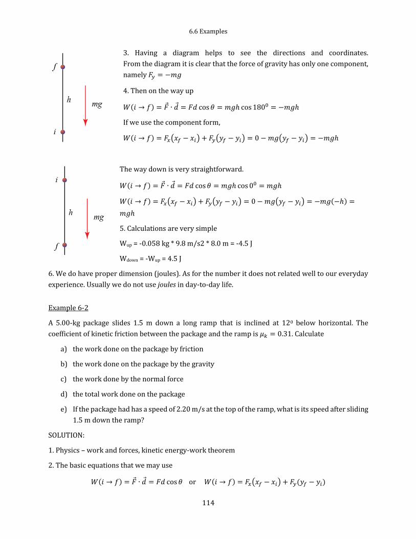
6.6 Examples
114
3. Having a diagram helps to see the directions and coordinates.
From the diagram it is clear that the force of gravity has only one component,
namely 𝐹𝑦 = −𝑚𝑔
4. Then on the way up
𝑊(𝑖 → 𝑓) = �⃗� ∙ 𝑑 = 𝐹𝑑 cos 𝜃 = 𝑚𝑔ℎ cos 1800 = −𝑚𝑔ℎ
If we use the component form,
𝑊(𝑖 → 𝑓) = 𝐹𝑥(𝑥𝑓 − 𝑥𝑖) + 𝐹𝑦(𝑦𝑓 − 𝑦𝑖) = 0 − 𝑚𝑔(𝑦𝑓 − 𝑦𝑖) = −𝑚𝑔ℎ
The way down is very straightforward.
𝑊(𝑖 → 𝑓) = �⃗� ∙ 𝑑 = 𝐹𝑑 cos 𝜃 = 𝑚𝑔ℎ cos 00 = 𝑚𝑔ℎ
𝑊(𝑖 → 𝑓) = 𝐹𝑥(𝑥𝑓 − 𝑥𝑖) + 𝐹𝑦(𝑦𝑓 − 𝑦𝑖) = 0 − 𝑚𝑔(𝑦𝑓 − 𝑦𝑖) = −𝑚𝑔(−ℎ) =
𝑚𝑔ℎ
5. Calculations are very simple
Wup = -0.058 kg * 9.8 m/s2 * 8.0 m = -4.5 J
Wdown = -Wup = 4.5 J
6. We do have proper dimension (joules). As for the number it does not related well to our everyday
experience. Usually we do not use joules in day-to-day life.
Example 6-2
A 5.00-kg package slides 1.5 m down a long ramp that is inclined at 120 below horizontal. The
coefficient of kinetic friction between the package and the ramp is 𝜇𝑘 = 0.31. Calculate
a) the work done on the package by friction
b) the work done on the package by the gravity
c) the work done by the normal force
d) the total work done on the package
e) If the package had has a speed of 2.20 m/s at the top of the ramp, what is its speed after sliding
1.5 m down the ramp?
SOLUTION:
1. Physics – work and forces, kinetic energy-work theorem
2. The basic equations that we may use
𝑊(𝑖 → 𝑓) = �⃗� ∙ 𝑑 = 𝐹𝑑 cos 𝜃 or 𝑊(𝑖 → 𝑓) = 𝐹𝑥(𝑥𝑓 − 𝑥𝑖) + 𝐹𝑦(𝑦𝑓 − 𝑦𝑖)

6. Kinetic Energy, Work, Power
115
∆𝐾 = 𝐾𝑓 − 𝐾𝑖 = ∫ �⃗� ∙ 𝑑𝑟𝑓
𝑖
= 𝑊(𝑖 → 𝑓)
3. Having a proper diagram would help to avoid confusion
with directions and angles.
Let’s choose the coordinate system such as the incline
surface is along x-coordinate. It makes easier to evaluate
the work along the surface.
For every force we have following components
Friction: 𝑓𝑥 = −𝜇𝑁𝑦 𝑓𝑦 = 0
Gravity: 𝐹𝑔𝑥 = 𝑚𝑔 sin 𝜃 𝐹𝑔𝑦 = −𝑚𝑔 cos 𝜃
Normal: 𝑁𝑥 = 0 𝑁𝑦 = −𝐹𝑔𝑦 = 𝑚𝑔 cos 𝜃
(Note that you may consider using Newton’s second law to find a connection between the forces if
you are not sure in the above force components).
4. Let’s use the component form for the work
𝑊(𝑖 → 𝑓) = 𝐹𝑥(𝑥𝑓 − 𝑥𝑖) + 𝐹𝑦(𝑦𝑓 − 𝑦𝑖)
with a notation 𝑑 = 𝑥𝑓 − 𝑥𝑖 and also note that 𝑦𝑓 − 𝑦𝑖 = 0 in our coordinate system.
The work done by friction 𝑊𝑓 = 𝐹𝑥(𝑥𝑓 − 𝑥𝑖) + 𝐹𝑦(𝑦𝑓 − 𝑦𝑖) = −𝜇𝑚𝑔 cos 𝜃 𝑑 + 0 ∙ 0 = −𝜇𝑚𝑔𝑑 cos 𝜃
The work done by gravity 𝑊𝑔 = 𝐹𝑥(𝑥𝑓 − 𝑥𝑖) + 𝐹𝑦(𝑦𝑓 − 𝑦𝑖) = 𝑚𝑔 sin 𝜃 𝑑 − 𝑚𝑔 cos 𝜃 ∙ 0 = 𝑚𝑔𝑑 sin 𝜃
The work done by normal force 𝑊𝑁 = 𝐹𝑥(𝑥𝑓 − 𝑥𝑖) + 𝐹𝑦(𝑦𝑓 − 𝑦𝑖) = 0 ∙ 𝑑 + 𝑚𝑔 cos 𝜃 ∙ 0 = 0
The total work done by all forces is 𝑊 = 𝑊𝑓 + 𝑊𝑔 + 𝑊𝑁
The speed at the end of the ramp
1
2𝑚𝑣𝑓
2 −1
2𝑚𝑣𝑖
2 = 𝑊 or 𝑣𝑓 = √𝑣𝑖2 + 2𝑊/𝑚
5. Calculations
𝑊𝑓 = −0.31 ∙ 5 𝑘𝑔 ∙ 9.8 𝑚 𝑠2⁄ ∙ 1.5 𝑚 ∙ cos 120 = −22.3 𝐽
𝑊𝑔 = 5 𝑘𝑔 ∙ 9.8 𝑚 𝑠2⁄ ∙ 1.5 𝑚 ∙ sin 120 = 15.3 𝐽
𝑊𝑛 = 0 𝐽
𝑊 = 𝑊𝑓 + 𝑊𝑔 + 𝑊𝑁 = −7.0 𝐽
𝑣𝑓 = √(2.2 𝑚 𝑠⁄ )2 − 2 ∙ 7 𝐽 5 𝑘𝑔⁄ = 1.4 𝑚 𝑠⁄

6.6 Examples
116
6. We have correct dimensions for the work. Let’s check the last term for the speed (under the square
root) [J]/[kg] = kg·m2/s2/kg = m2/s2 that is v2 (correct).
We may also notice that the final speed is less that the initial speed. It corresponds to a case when the
frictional force is larger than gravity along the ramp thus doing more work.
Example 6-3
A 6.0 kg cat sleeps on a mat. A dog pulls the mat across the floor using a rope that makes 200 above
the floor. The tension is a constant 20.0 N and the coefficient of friction is 0.20. Find cat’s speed after
being pulled 2.0 m.
SOLUTION:
1. Physics –kinetic energy-work theorem
2. The basic equations that we may use
𝑊(𝑖 → 𝑓) = 𝐹𝑥(𝑥𝑓 − 𝑥𝑖) + 𝐹𝑦(𝑦𝑓 − 𝑦𝑖)
𝐾𝑓 − 𝐾𝑖 =𝑚𝑣𝑓
2
2−
𝑚𝑣𝑖2
2= 𝑊(𝑖 → 𝑓)
3. The free-body diagram on the right has all the forces
in place. For every force we have following components
Tension: 𝑇𝑥 = 𝑇 cos 𝜃 , 𝑇𝑦 = 𝑇 sin 𝜃
Gravity: 𝐹𝑔𝑥 = −𝑚𝑔, 𝐹𝑔𝑦 = 0
Normal force: 𝑁𝑥 = 0, 𝑁𝑦
Friction: 𝑓𝜇𝑥 = −𝜇𝑁𝑦, 𝑓𝜇𝑦 = 0
4. We work only with the 𝑥 −components because there is no displacement in the 𝑦 − direction.
First we need to find the normal force from second newton’s law for
First we need to find the normal force from second newton’s law for 𝑦 −components
𝑁𝑦 + 𝑇 sin 𝜃 − 𝑚𝑔 = 0, 𝑁𝑦 = 𝑚𝑔 − 𝑇 sin 𝜃 , 𝑓𝜇𝑥 = −𝜇(𝑚𝑔 − 𝑇 sin 𝜃)
now
𝑚𝑣𝑓2
2= (𝑇 cos 𝜃 − 𝜇(𝑚𝑔 − 𝑇 sin 𝜃))𝑥𝑓 , 𝑣𝑓
2 =2
𝑚(𝑇 cos 𝜃 − 𝜇(𝑚𝑔 − 𝑇 sin 𝜃))𝑥𝑓
5. Calculations
𝑣𝑓 = 2.4 𝑚/𝑠
6. The answer seems convincing.
6. Kinetic Energy, Work, Power
117
Example 6-4
Your job is to lift 30-kg crates a vertical distance of 0.90 m from the ground onto the bed of a truck.
How many crates you have to load onto the truck in 1 minute for the average power output you use
to lift the crates to equal 1.0 hp? (Working like a horse!)
SOLUTION:
1. Physics – power, work and forces
2. Basic equations: we need average power (because we speak about relatively large time intervals)
as well work done by you against gravity
𝑃𝑎𝑣𝑔 =𝑊
Δ𝑡 (average power) 𝑊𝑦𝑜𝑢 = −(−𝑚𝑔ℎ) = 𝑚𝑔ℎ
3. Having the power and time we may calculate how much work can be done with this power. Dividing
this work by the work to lift one box we can find how many boxes we should lift in one minute.
4. Total work with given power 𝑊 = 𝑃𝑎𝑣𝑔Δ𝑡, and the work to lift one box 𝑊𝑏𝑜𝑥 = 𝑚𝑔ℎ
𝑁𝑏𝑜𝑥𝑒𝑠 =𝑊
𝑊𝑏𝑜𝑥
5. Calculations
First we evaluate power in watt
1.0 ℎ𝑝 = 1.0 ℎ𝑝746 𝑊
1 ℎ𝑝= 746 𝑊
𝑁 =746 𝑊 ∙ 60 𝑠
30 𝑘𝑔 ∙ 9.8 𝑚 𝑠2⁄ ∙ 0.9 𝑚 = 169 boxes
6. Let’s check the dimensions. The numerator [W]*[s] = [J] = kg·m2/s2, the denominator is kg·m2/s2
(OK)
It is clear that we cannot load so many heavy boxes in one minute, thus we cannot work like a horse!

7.1 Potential energy and conservative forces
118
7 Conservation of Energy
7.1 Potential energy and conservative forces
In nature there are certain forces which have a very remarkable property which we call
"conservative" (no political ideas involved). If we calculate how much work is done by a force in
moving an object from one point to another along some curved path, in general the work depends
upon the path; but, in special cases it does not. If it does not depend upon the path, we say that the
force is a conservative force.
Strictly speaking there are two conditions for a force to be conservative. A force �⃗� acting on a particle
is conservative if and only if it satisfy two conditions:
1. �⃗� depends only on the particle’s position 𝑟 (and not on the velocity �⃗�, or the time 𝑡, or any
other variable) that is �⃗� = �⃗�(𝑟).
2. For any two points 𝑟1 and 𝑟2, the integral
∫ �⃗� ∙ 𝑑𝑟𝑟2
𝑟1
is the same for all paths between points 1 and 2, or work 𝑊(1 → 2) done by �⃗� is
independent of paths between points 1 and 2.
The reason for the name conservative and for the importance of the concept is this: if all forces acting
on an object are conservative, we can define a quantity called the potential energy, denoted 𝑈(𝑟), a
function of only position, with the property that the total mechanical energy
𝐸 = 𝐾 + 𝑈(𝑟) (7.1)

7. Conservation of Energy
119
is conserved.
To define the potential energy 𝑈(𝑟) corresponding to a given conservative force, we first choose a
reference point 𝑟0 at which 𝑈 is defined to be zero (e.g. in the case of gravity near the earth's surface,
we often define 𝑈 to be zero at ground level.) We then define 𝑈(𝑟), the potential energy at an arbitrary
point 𝑟, to be
𝑈(𝑟) = − ∫ 𝐹(𝑟′)𝑑𝑟′𝑟
𝑟0
= −𝑊(𝑟0 → 𝑟) (7.2)
In words, 𝑈(𝑟) is minus the work done by �⃗� if the particle moves from
the reference point 𝑟0 to the point of interest 𝑟. Notice that the definition
above only makes sense because of the property (2) of conservative
forces. If the integral were different for different paths, it would not
define a unique function 𝑈(𝑟).
We can now derive a crucial expression for the work done by �⃗� in terms
of the potential energy 𝑈(𝑟). Let 𝑟1 and 𝑟2 be any two points as in Figure
on the right. If 𝑟0 is the reference point at which 𝑈 is zero, then it is clear
from that
𝑊(𝑟0 → 𝑟2) = 𝑊(𝑟0 → 𝑟1) + 𝑊(𝑟1 → 𝑟2)
and hence
𝑊(𝑟1 → 𝑟2) = 𝑊(𝑟0 → 𝑟2) − 𝑊(𝑟0 → 𝑟1)
Each of the two terms on the right is (minus) the potential energy at the corresponding point. Thus
we have proved that the work on the left is just the difference of these two potential energies:
𝑊(𝑟1 → 𝑟2) = −[𝑈(𝑟2) − 𝑈(𝑟1)] = −Δ𝑈
The usefulness of this result emerges when we combine it with the Kinetic Energy – Work theorem
∆𝐾 = 𝐾2 − 𝐾1 = ∫ �⃗� ∙ 𝑑𝑟2
1
= 𝑊(1 → 2)
Namely we can now write
Δ𝐾 = −Δ𝑈 (7.3)
or, moving the right side across to the left
Δ(𝐾 + 𝑈) = 0
That is, the mechanical energy
𝐸 = 𝐾 + 𝑈 (7.4)
does not change as the particle moves from 𝑟1 to 𝑟2. Since the points 𝑟1 and 𝑟2 were any two points on
the particle's trajectory, we have the important conclusion: If the force on a particle is conservative,

7.1 Potential energy and conservative forces
120
then the particle's mechanical energy never changes; that is, the particle's energy is conserved, which
explains the use of the adjective "conservative."
So far we have established the conservation of energy for a particle subject to a single conservative
force. If the particle is subject to several forces, all of them conservative, our result generalizes easily.
7.1.1 Force as a gradient of potential energy
We have seen that the potential energy 𝑈 (𝑟) corresponding to a force �⃗� can be expressed as an
integral of �⃗�. This suggests that we should be able to write �⃗� as some kind of derivative of 𝑈 (𝑟). Using
some mathematics we can show that
�⃗� = −∇⃗⃗⃗𝑈 = −𝑥𝜕𝑈
𝜕𝑥− �̂�
𝜕𝑈
𝜕𝑦− �̂�
𝜕𝑈
𝜕𝑧 (7.6)
This expression gives formal definition of potential energy 𝑈. In one-dimensional case, this
connection between force and potential energy is particularly simple:
𝐹𝑥 = −𝑑𝑈
𝑑𝑥 (7.7)
Let’s note that 𝑈 is always arbitrary to within an additive constant, because taking a derivative of a
constant function gives zero:
∇⃗⃗⃗(𝑈 + 𝑐) = ∇⃗⃗⃗𝑈 + ∇⃗⃗⃗𝑐 = ∇⃗⃗⃗𝑈
Therefore, the force �⃗� (which is an “explicitly observable” quantity) does not change if we add a
constant to the “auxiliary” quantity 𝑈. In other words, the potential energy 𝑈 gives rise to the same
force as the potential energy 𝑈 + 𝑐. Since it is the force (rather than the potential energy) that is
physically observable, we say that these two potential energies are equivalent.
It is not the absolute value of potential energy that is important. Rather, it is the change in potential
energy over distance (the gradient) that creates force and is, therefore, important.
A consequence of this observation is that, for a given problem, the “zero” of potential can be chosen
arbitrarily as a matter of convenience.
Principle of Conservation of Energy for One Particle
If all of the 𝑛 forces �⃗�𝑖 (𝑖 = 1, . . . , 𝑛) acting on a particle are conservative, each
with its corresponding potential energy 𝑈𝑖(𝑟), the total mechanical energy,
defined as
𝐸 = 𝐾 + 𝑈1(𝑟) + 𝑈2(𝑟) + ⋯ + 𝑈𝑛(𝑟) (7.5)
is constant in time.

7. Conservation of Energy
121
7.2 Gravitational and elastic potential energies
In University Physics I we usually deal with two conservative forces, namely gravity and elastic
(spring) force. In University Physics II we add the Coulomb force on electric charge.
7.2.1 Gravitational potential energy
If we are not going to heights comparable with the radius of the earth, then the force of gravity is a
constant vertical force 𝐹𝑦 = −𝑚𝑔. Then
𝐹𝑦 = −𝑚𝑔 = −𝑑𝑈𝑔
𝑑𝑦
𝑑𝑈𝑔 = 𝑚𝑔𝑑𝑦, then ∫ 𝑑𝑈𝑔 = ∫ 𝑚𝑔𝑑𝑦𝑦
0
and finally
𝑈𝑔(𝑦) = 𝑚𝑔𝑦 (7.8)
Let’s consider a change in gravitational potential energy between two points using the definition of
the work based on the integral from a force3. Since there is only one y-component
Δ𝑈𝑔 = 𝑈𝑔𝑓 − 𝑈𝑔𝑖 = − ∫ 𝐹𝑦𝑑𝑦𝑦𝑓
𝑦𝑖
= ∫ 𝑚𝑔𝑑𝑦𝑦𝑓
𝑦𝑖
= 𝑚𝑔(𝑦𝑓 − 𝑦𝑖)
Δ𝑈𝑔 = 𝑚𝑔(𝑦𝑓 − 𝑦𝑖) (7.9)
As we noted above, only changes in potential energy are physically meaningful. However to simplify
calculations we may select a reference point 𝑦𝑖 where 𝑈𝑖 = 0, then 𝑈(𝑦) = 𝑚𝑔𝑦.
Good to remember: The gravitational potential energy associated with a particle-Earth system
depends ONLY on the vertical position 𝑦 (or height) of the particle relative to the reference position
(𝑦 = 0), not on the horizontal position. And again, only differences in potential energy count.
7.2.2 Elastic (spring) potential energy
For the elastic restoring force of a spring 𝐹 = −𝑘𝑥 is a good approximation for many springs (Hooke’s
law) where 𝑘 is a spring constant (a SI unit for 𝑘 is N/m).
𝐹𝑥 = −𝑘𝑥 ⇒ −𝑑𝑈𝑠
𝑑𝑥= −𝑘𝑥
𝑑𝑈𝑠 = 𝑘𝑥𝑑𝑥 ⇒ ∫ 𝑑𝑈𝑠 = ∫ 𝑘𝑥𝑑𝑥𝑥
0
then
3 from chapter 6: 𝑊(𝑖 → 𝑓) = ∫ �⃗� ∙ 𝑑𝑟𝑓
𝑖= ∫ 𝐹𝑥𝑑𝑥
𝑥𝑓
𝑥𝑖+ ∫ 𝐹𝑦𝑑𝑦
𝑦𝑓
𝑦𝑖. Since work and the potential energy
are connected 𝑊(𝑖 → 𝑓) = −[𝑈(𝑟𝑓) − 𝑈(𝑟𝑖)] = −Δ𝑈, then Δ𝑈 = − ∫ 𝐹𝑥𝑑𝑥𝑥𝑓
𝑥𝑖− ∫ 𝐹𝑦𝑑𝑦
𝑦𝑓
𝑦𝑖

7.3 Non-conservative forces
122
𝑈𝑠 =1
2𝑘𝑥2 (7.10)
The zero of potential energy is at the point 𝑥 = 0, the equilibrium position of the spring. Again we
could add any constant we wish to 𝑈𝑠 but not to 𝑥.
Now we do the same using Δ𝑈 = − ∫ 𝐹𝑥𝑑𝑥𝑥𝑓
𝑥𝑖− ∫ 𝐹𝑦𝑑𝑦
𝑦𝑓
𝑦𝑖
Δ𝑈 = 𝑈𝑓 − 𝑈𝑖 = − ∫ 𝐹𝑥𝑑𝑥𝑥𝑓
𝑥𝑖
= ∫ 𝑘𝑥𝑑𝑥𝑥𝑓
𝑥𝑖
= 𝑘 ∫ 𝑥𝑑𝑥𝑥𝑓
𝑥𝑖
=1
2𝑘𝑥𝑓
2 −1
2𝑘𝑥𝑖
2
Δ𝑈𝑠 =1
2𝑘𝑥𝑓
2 −1
2𝑘𝑥𝑖
2 (7.11)
Important: The reference point for the spring potential energy must be the equilibrium point.
7.3 Non-conservative forces
As a matter of fact, all the fundamental forces in nature appear to be conservative. This is not a
consequence of Newton's laws. In fact, so far as Newton himself knew, the forces could be
nonconservative, as friction apparently is. When we say friction apparently is, we are taking a modern
view, in which it has been discovered that all the deep forces, the forces between the particles at the
most fundamental level, are conservative.
When we study matter in the finest detail at the atomic level, it is not always easy to separate the total
energy of a thing into two parts, kinetic energy and potential energy, and such separation is not
always necessary. In many situations, it is practical to replace vast amount of conservative forces
between particles on a single nonconservative force. Then all these different forms of internal energy
are sometimes considered as "lost". When friction is present it is not true that kinetic energy is lost,
even though a sliding object stops and the kinetic energy seems to be lost. The kinetic energy is not
lost because, of course, the atoms inside are jiggling with a greater amount of kinetic energy than
before, and although we cannot see that, we can measure it by determining the temperature. Of course
if we disregard the heat energy, then the conservation of energy theorem will appear to be false.
If some of the forces on our particle are nonconservative (like friction), then we cannot define
corresponding potential energies; nor can we define a conserved mechanical energy.
Nevertheless, we can define potential energies for all of the forces that are conservative, and then
recast the Kinetic Energy – Work theorem in a form that shows how the nonconservative forces
change the particle's mechanical energy. First, we divide the net force on the particle into two parts,
the conservative part �⃗�𝑐𝑜𝑛𝑠 and the nonconservative part �⃗�𝑛𝑐. For conservative forces we can define a
potential energy, which we'll call just 𝑈. By the Kinetic Energy – Work theorem, the change in kinetic
energy between any two times is
Δ𝐾 = 𝑊𝑐𝑜𝑛𝑠 + 𝑊𝑛𝑐

7. Conservation of Energy
123
The first term on the right is just −Δ𝑈 and can be moved to the left side to give Δ(𝐾 + 𝑈) = 𝑊𝑛𝑐. If
we define the mechanical energy as 𝐸 = 𝐾 + 𝑈, then we see that Δ𝐸 = Δ(𝐾 + 𝑈) = 𝑊𝑛𝑐 or
𝐾𝑖 + 𝑈𝑖 = 𝐾𝑓 + 𝑈𝑓 − 𝑊𝑛𝑐 (7.12)
Mechanical energy is no longer conserved, but we have the next best thing. The mechanical energy
changes to precisely the extent that the nonconservative forces do work on our particle. In many
problems, the only nonconservative force is the force of sliding friction, which usually does negative
work. (The frictional force 𝑓 is in the direction opposite to the motion, so the work done by a frictional
force is negative.) In this case 𝑊𝑛𝑐 is negative and the object loses mechanical energy in the amount
"stolen" by friction 𝑊𝑛𝑐 = 𝑊𝑓𝑟 = −𝑓𝜇 𝑑.
Let’s consider as an example a block sliding down an incline, namely a block of mass 𝑚 accelerating
from rest down incline that has a coefficient of friction 𝜇 and is at angle 𝜃 from horizontal. Let’s find
its speed 𝑣 when it reaches the bottom of the slope, a distance 𝑑 from its starting point 𝑂.
The setup and the forces on the block are
shown in Figure. The three forces on the block
are its weight, �⃗⃗⃗� = �⃗�𝑔 = 𝑚�⃗�, the normal force
of the incline, �⃗⃗⃗�, and the frictional force 𝑓,
whose magnitude to be 𝑓𝜇 = 𝜇𝑚𝑔 cos 𝜃. The
force of gravity is conservative, and the
corresponding potential energy is 𝑈 =
𝑚𝑔𝑦 where 𝑦 is the block's vertical height
above the bottom of the slope (if we choose the
zero of potential energy at the bottom). The
normal force does no work, since it is perpendicular to the direction of motion, so will not contribute
to the energy balance. The frictional force does work 𝑊𝑓𝑟 = −𝑓𝑑 = −𝜇𝑚𝑔𝑑 cos 𝜃. The change in
kinetic energy is
𝐾𝑓 − 𝐾𝑖 =1
2𝑚𝑣2
and the change in potential energy is
Δ𝑈 = 𝑈𝑓 − 𝑈𝑖 = −𝑚𝑔ℎ = −𝑚𝑔𝑑 sin 𝜃
Then
Δ𝐸 = Δ(𝐾 + 𝑈) = 𝑊𝑛𝑐
1
2𝑚𝑣2 − 𝑚𝑔𝑑 sin 𝜃 = −𝜇𝑚𝑔𝑑 cos 𝜃
Solving for 𝑣 we find
𝑣 = √2𝑔𝑑(sin 𝜃 − 𝜇 cos 𝜃)

7.4 Potential energy diagrams
124
As usual, you should check that this answer agrees with common sense. For example, does it give the
expected answer when 𝜃 = 900? What about 𝜃 = 00?
7.4 Potential energy diagrams
A useful feature of one-dimensional systems is that with only one independent variable (𝑥) we can
plot the potential energy 𝑈(𝑥), and, as we shall see, this makes it easy to visualize the behavior of the
system.
If we plot the potential energy against 𝑥 as in Figure, we can easily see qualitatively how the object
has to behave. The direction of the net force is
given by
𝐹𝑥 = −𝑑𝑈
𝑑𝑥
as "downhill" on the graph of 𝑈(𝑥) - to the left
at 𝑥1 and to the right at 𝑥2 It follows that the
object always accelerates in the "downhill"
direction - a property that reminds one of the
motion of a roller coaster, which also always accelerates downhill. This analogy is not an accident:
For a roller coaster, 𝑈(𝑥) is 𝑚𝑔ℎ (where ℎ is the height above ground) and the graph of 𝑈(𝑥) against
𝑥 has the same shape as a graph of ℎ against 𝑥, which is just a picture of the track. For any one-
dimensional system, we can always think about the graph of 𝑈(𝑥) as a picture of a roller coaster, and
common sense will generally tell us the kind of motion that is possible at different places
At points, such as 𝑥3 and𝑥4, where 𝑑𝑈/𝑑𝑥 = 0 and 𝑈(𝑥) is minimum or maximum, the net force is
zero, and the object can remain in equilibrium. That is, the condition 𝑑𝑈/𝑑𝑥 = 0 characterizes points
of equilibrium. At 𝑥3, where 𝑑2𝑈 𝑑𝑥2⁄ > 0 and 𝑈(𝑥) is minimum, a small displacement from
equilibrium causes a force which pushes the object back to equilibrium (back to the left on the right
of 𝑥3, back to the right on the left of 𝑥3). In other words, equilibrium points where 𝑑2𝑈 𝑑𝑥2⁄ > 0 and
𝑈(𝑥) is minimum are points of stable equilibrium. At equilibrium points like 𝑥4 where 𝑑2𝑈 𝑑𝑥2⁄ < 0
and 𝑈(𝑥)is maximum, a small displacement leads to a force away from equilibrium, and the
equilibrium is unstable.
If the object is moving then its kinetic energy is positive and its total energy is necessarily greater
than 𝑈(𝑥). For example, suppose the object is moving somewhere near the equilibrium point = 𝑏.
Its total energy has to be greater than 𝑈(𝑏)
and could, for example, equal the value
shown as 𝐸 in that figure. If the object
happens to be on the right of b and moving
toward the right, its potential energy will
increase and its kinetic energy must
therefore decrease until the object reaches

7. Conservation of Energy
125
the turning point labeled 𝑐, where 𝑈(𝑐) = 𝐸 and the kinetic energy is zero. At 𝑥 = 𝑐 the object stops
and, with the force back to the left, it accelerates back toward 𝑥 = 𝑏. It cannot now stop until once
again the Kinetic energy is zero, and this occurs at the turning point 𝑎, where 𝑈(𝑎) = 𝐸 and the object
accelerates back to the right. Since the whole cycle now repeats itself, we see that if the object starts
out between two hills and its energy is lower than the crest of both hills, then the object is trapped in
the valley or "well" and oscillates indefinitely between the two turning points where 𝑈(𝑥) = 𝐸.
Suppose the cart again starts out between the two hills but with energy higher than the crest of the
right hill though still lower than the left. In this case, it will escape to the right since 𝐸 > 𝑈(𝑥)
everywhere on the right, and it can never stop once it is moving in that direction. Finally, if the energy
is higher than both hills, the cart can escape in either direction.
These considerations play an important role in many fields.
7.5 Guidelines for solving most common problems in “Conservation of energy”
126
7.5 Guidelines for solving most common problems in “Conservation of energy”
All problems can be divided into two groups: 1) “pure conservation of energy” problems, when one
only need to use conservation of energy to find an answer, and 2) “ combined” problems, that may
also include 1D motion or 2D projectile motion, or circular motion (pendulums, loops).
Here is a reference table for equations.
Energy Equation Comments
The kinetic energy 𝐾 =1
2𝑚𝑣2
The gravitational potential
energy (particle-Earth) 𝑈𝑔(𝑦) = 𝑚𝑔𝑦
if the reference frame is set
as 𝑦𝑖 = 0
The elastic potential energy 𝑈𝑠(𝑥) =1
2𝑘𝑥2
where the reference is set at
relaxed length 𝑥 = 0
The total mechanical
energy 𝐾𝑖 + 𝑈𝑖 = 𝐾𝑓 + 𝑈𝑓
The conservation of energy 𝐾𝑖 + 𝑈𝑖 = 𝐾𝑓 + 𝑈𝑓 + 𝑓𝑘𝑑 (with frictional force)
Let’s concentrate on applying conservation of energy to a single object. Unlike dealing with forces, the
procedure is rather simple for solving problems in Physics I.
Point 1: You start with writing down the law of conservation of energy in most detailed form
1
2𝑚𝑣𝑖
2 + 𝑚𝑔𝑦𝑖 +1
2𝑘𝑥𝑖
2 =1
2𝑚𝑣𝑓
2 + 𝑚𝑔𝑦𝑓 +1
2𝑘𝑥𝑓
2 + 𝑓𝑘𝑑
Attention:
While you may choose any reference point for the gravitational potential energy, the
reference point for the spring potential energy MUST be the equilibrium point.
If you have a spring, its orientation can be horizontal (then we use (1 2⁄ )𝑘𝑥2), or vertical (at
that time we use (1 2⁄ )𝑘𝑦𝑠2), or under some angle (for example, a spring on an incline).
Most mistakes students do in problems with both gravitational and spring energies. The
cause of mistakes is not choosing properly reference points for the two energies.
Point 2: You analyze what energy you have in your problem, and keep only relevant terms in the
above equation.
Point 3: Finally you have one equation with one unknown. That is a simple algebra task.
In case of two connected objects you include all energies for both objects into a single equation (we
use conservation of energy for a system). For clarity let’s keep only kinetic and gravitational potential
energy (you may easily add the spring energy and energy lost to friction when needed)

7. Conservation of Energy
127
1
2𝑚𝑣1𝑖
2 + 𝑚𝑔𝑦1𝑖 +1
2𝑚𝑣2𝑖
2 + 𝑚𝑔𝑦2𝑖 =1
2𝑚𝑣1𝑓
2 + 𝑚𝑔𝑦1𝑓 +1
2𝑚𝑣2𝑓
2 + 𝑚𝑔𝑦2𝑓
7.6 Examples
Example 7-1
You throw a tennis ball straight up with initial speed 𝑣𝑖 = 15.0 𝑚/𝑠. How high does it go above the
point where you release it? Ignore air resistance
SOLUTION:
1. Physics – gravity, motion, conservation of
energy
2. The basic equation
𝐾𝑖 + 𝑈𝑖 = 𝐾𝑓 + 𝑈𝑓 + 𝑓𝑘𝑑
3. In this problem there is only one force affecting
the flight, namely gravity, therefore we can write
1
2𝑚𝑣𝑖
2 + 𝑚𝑔𝑦𝑖 =1
2𝑚𝑣𝑓
2 + 𝑚𝑔𝑦𝑓
with the given conditions 𝑣𝑓 = 0 and choosing the reference point for gravity as 𝑦𝑖 = 0
1
2𝑚𝑣𝑖
2 + 0 = 0 + 𝑚𝑔𝑦𝑓
4. The equation above produces an instant solution for the final vertical position
𝑦𝑓 =𝑣𝑖
2
2𝑔
5. Calculations
𝑦𝑓 =(15.0 𝑚 𝑠⁄ )2
2 ∙ 9.8 𝑚 𝑠2⁄= 11.5 𝑚
6. We have got a proper dimension (meters). The numerical answer seems reasonable.
Example 7-2
You are driving at 55 mph when the road suddenly descends 90 ft into a valley. You take your foot off
the accelerator and coast down the hill. Just as you reach the bottom you see the policeman hiding
behind the speed limit sign that reads “70 mph”. Are you going to get a speeding ticket? (Neglect air
and rolling resistance)
SOLUTION:

7.6 Examples
128
1. Physics – gravity, motion, conservation of mechanical energy
2. The basic equation
𝐾𝑖 + 𝑈𝑖 = 𝐾𝑓 + 𝑈𝑓
3. Then
1
2𝑚𝑣𝑖
2 + 𝑚𝑔𝑦𝑖 =1
2𝑚𝑣𝑓
2 + 𝑚𝑔𝑦𝑓
Choosing the reference point for gravity as 𝑦𝑓 = 0 (at the sign 70 mph)
1
2𝑚𝑣𝑖
2 + 𝑚𝑔𝑦𝑖 =1
2𝑚𝑣𝑓
2
4. Solving for the final speed gives
𝑣𝑓 = √𝑣𝑖2 + 2𝑔𝑦𝑖
5. Calculations
𝑣𝑖 = 55 𝑚𝑝ℎ = 55 (𝑚𝑖𝑙𝑒
ℎ𝑜𝑢𝑟) (
1609 𝑚
1 𝑚𝑖𝑙𝑒) (
1 ℎ𝑜𝑢𝑟
3600 𝑠) = 24.6 𝑚/𝑠
𝑦𝑖 = 90 𝑓𝑡 = 90 𝑓𝑡0.348 𝑚
1 𝑓𝑡= 27.4 𝑚
𝑣𝑓 = 33.8 𝑚 𝑠⁄ = 75.6 𝑚𝑝ℎ
6. We have got a proper dimension (speed in m/s). The numerical answer seems reasonable.

7. Conservation of Energy
129
Example 7-3
A block is released from rest at the top of a frictionless ramp, at height H1 (point 𝑂) above the base of
the ramp. The ramp ends at height H2 above the base, so that the block flies off and follows a two-
dimensional projectile motion until it hits the ground. Find the speed of the block in terms of the given
variables when it strikes the ground.
SOLUTION
1. Physics – motion with acceleration on incline, projectile motion, conservation of energy.
We could try to solve the problem in old-fashioned way. First we solve the “incline” problem, or
motion with acceleration on the incline after using Newton’s second law to find the acceleration. Then
we solve the projectile motion problem. However, it is not only a long way to go; it is not possible in
this case since we are not given the horizontal size of the ramp.
Therefore we are going to use conservation of energy
2. The basic equation
𝐾𝑖 + 𝑈𝑖 = 𝐾𝑓 + 𝑈𝑓 + 𝑓𝑘𝑑
3. In this problem, there is only one force affecting the motion, namely gravity. We could split the
motion into two phases, namely from the top of the ramp H1 to the end at height H2, and them the
motion to the ground. But it is unnecessary. We may just consider the initial (on the top of the ramp)
and final (on the ground) configurations, where 𝑦𝑖 = 𝐻1, 𝑣𝑖 = 0 and 𝑦𝑓 = 0. Then the equation
1
2𝑚𝑣𝑖
2 + 𝑚𝑔𝑦𝑖 =1
2𝑚𝑣𝑓
2 + 𝑚𝑔𝑦𝑓
is greatly simplified
0 + 𝑚𝑔𝐻1 =1
2𝑚𝑣𝑓
2 + 0
4. The speed of the block as it strikes the ground is
𝑣𝑓 = √2𝑔𝐻1
5. No calculations (no data)

7.6 Examples
130
6. Let’s check dimension for the speed √𝑚
𝑠2 𝑚 = √𝑚2
𝑠2 =𝑚
𝑠 correct, we got it as m/s.
The same speed is the same as dropping the block vertically from the same height.
Note: In the same way we may solve a roller coaster problem. If there is no resistance/friction, then
the profile does not matter.
Example 7-4
A child’s toy shoots a marble with a horizontal spring (spring constant k=11N/m). The marble has a
mass of 16 g. If the spring is compressed 3.4 cm and then released, what is the speed of the marble
when it leaves the spring? Assume that the marble experiences no resistive forces.
SOLUTION
1. Physics – spring, motion, conservation of energy.
2. The basic equation
𝐾𝑖 + 𝑈𝑖 = 𝐾𝑓 + 𝑈𝑓 + 𝑓𝑘𝑑
3. In this problem we have one only force, namely the spring force
1
2𝑚𝑣𝑖
2 +1
2𝑘𝑥𝑖
2 =1
2𝑚𝑣𝑓
2 +1
2𝑘𝑥𝑓
2
Using the conditions 𝑣𝑖 = 0, 𝑥𝑓 = 0
0 +1
2𝑘𝑥𝑖
2 =1
2𝑚𝑣𝑓
2 + 0
4. Solving the equation for the final speed gives
𝑣𝑓 = √𝑘𝑥𝑖
2
𝑚
5. Calculations

7. Conservation of Energy
131
𝑣𝑓 = √(11 𝑁/𝑚)(−0.034 𝑚)2
0.016 𝑘𝑔= 0.89 𝑚/𝑠
6. Check dimensions
[N]=[kg]*[m]/[s]2 then for the speed
√𝑘𝑔 ∙ 𝑚
𝑠2
1
𝑚
𝑚2
𝑘𝑔= √
𝑚2
𝑠2=
𝑚
𝑠
correct!
The numerical answer seems reasonable to spring toys.
Example 7-5
As 18,000 kg F/A-18E/F Super Hornet lands on aircraft carrier USS Harry S. Truman (CVN-75), its tail
hook snags an arresting cable to slow it down. The cable stretches 80 m to stop the aircraft. Assume
that the cable is attached to a spring with spring constant 10,000 N/m, and the coefficient of static
friction between the aircraft’s tires and the deck is 0.80.
What was the plane’s landing speed?
SOLUTION
1. Physics – motion, spring force, friction, energy conservation
2. The basic equation 𝐾𝑖 + 𝑈𝑖 = 𝐾𝑓 + 𝑈𝑓 + 𝑓𝑘𝑑
3. For the problem in hand (the initial kinetic energy went into spring potential energy and friction)
we have
1
2𝑚𝑣𝑖
2 =1
2𝑘𝑥𝑓
2 + 𝜇𝑚𝑔𝑥
4. Solving for 𝑣𝑖
𝑣𝑖 = √𝑘𝑥𝑓
2
𝑚+ 2𝜇𝑔𝑥
5. Calculations
𝑣𝑖 = √10000 𝑁 𝑚⁄ (80 𝑚)2
18000 𝑘𝑔+ 2 ∙ 0.8 ∙ 9.8 𝑚 𝑠2⁄ ∙ 80 𝑚 = 69.3 𝑚 𝑠⁄
6. Let’s see the landing speed in mph 69.3 𝑚 𝑠⁄ = 155 𝑚𝑝ℎ. This is a very reasonable landing speed
for F-18 Super Hornet.

7.6 Examples
132
Example 7-6
A 10,000-kg runaway truck with failed brakes is moving 70 mph just before the driver steers the truck
up the runaway ramp with an inclination of 200. Assume that the coefficients of static and kinetic
friction between the ramp and the truck are 0.95 and 0.8 respectively. A driver slammed on his brakes.
What minimum length L must the ramp have to stop along it?
SOLUTION
1. Physics – three forces (gravity, friction, normal),
motion along an incline and energy.
This problem can be solved by either the old way4
(using Newton’s laws + one dimensional kinematics)
or using conservation of energy. Let’s use
conservation of energy.
2. The basic equation
𝐾𝑖 + 𝑈𝑖 = 𝐾𝑓 + 𝑈𝑓 + 𝑓𝑘𝑑
3. Working with conservation of energy we have to carefully choose the initial and final configurations
and reference points for potentials. In this problem our choice is rather straightforward. We choose
the initial point at the base of the ramp where 𝑦𝑖 = 0, then
1
2𝑚𝑣𝑖
2 + 𝑚𝑔𝑦𝑖 =1
2𝑚𝑣𝑓
2 + 𝑚𝑔𝑦𝑓 + 𝑓𝜇𝑑
where 𝑑 is the stopping distance.
The conditions 𝑣𝑓 = 0, 𝑦𝑓 = 𝑑 sin 𝜃, and the frictional force 𝑓𝜇 = 𝜇𝑠𝑁 = 𝜇𝑠𝑚𝑔 cos 𝜃 (see chapter 5 for
details). Note that we use the static coefficient assuming the brakes were not locked.
Then the conservation of energy can be written as
1
2𝑚𝑣𝑖
2 + 0 = 0 + 𝑚𝑔𝑑 sin 𝜃 + 𝜇𝑠𝑚𝑔𝑑 cos 𝜃
4. The equation above can be easily solved for 𝑑
𝑑 =𝑣𝑖
2
2𝑔(sin 𝜃 + 𝜇𝑠 cos 𝜃)
5. Calculations
70 𝑚𝑝ℎ = 70 𝑚𝑖𝑙𝑒
ℎ (
1609 𝑚
1 𝑚𝑖𝑙𝑒) (
1 ℎ
3600 𝑠) = 31 𝑚/𝑠
4 see example 5-4 in chapter 5
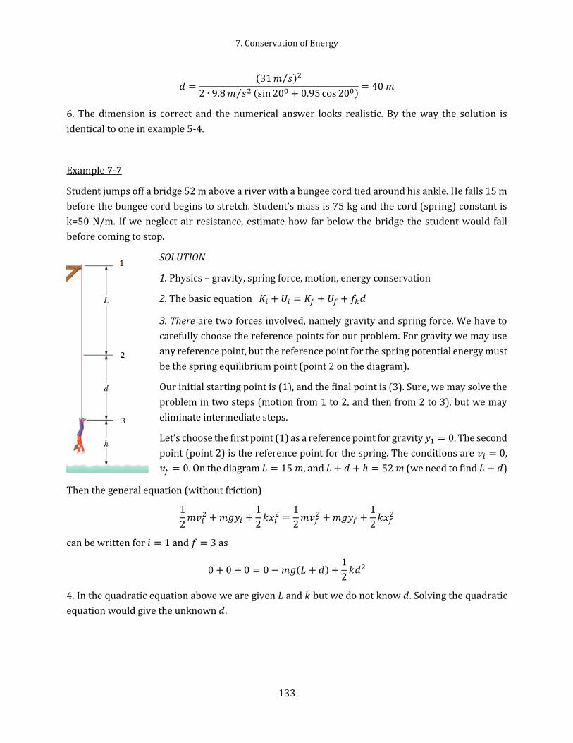
7. Conservation of Energy
133
𝑑 =(31 𝑚 𝑠⁄ )2
2 ∙ 9.8 𝑚 𝑠2⁄ (sin 200 + 0.95 cos 200)= 40 𝑚
6. The dimension is correct and the numerical answer looks realistic. By the way the solution is
identical to one in example 5-4.
Example 7-7
Student jumps off a bridge 52 m above a river with a bungee cord tied around his ankle. He falls 15 m
before the bungee cord begins to stretch. Student’s mass is 75 kg and the cord (spring) constant is
k=50 N/m. If we neglect air resistance, estimate how far below the bridge the student would fall
before coming to stop.
SOLUTION
1. Physics – gravity, spring force, motion, energy conservation
2. The basic equation 𝐾𝑖 + 𝑈𝑖 = 𝐾𝑓 + 𝑈𝑓 + 𝑓𝑘𝑑
3. There are two forces involved, namely gravity and spring force. We have to
carefully choose the reference points for our problem. For gravity we may use
any reference point, but the reference point for the spring potential energy must
be the spring equilibrium point (point 2 on the diagram).
Our initial starting point is (1), and the final point is (3). Sure, we may solve the
problem in two steps (motion from 1 to 2, and then from 2 to 3), but we may
eliminate intermediate steps.
Let’s choose the first point (1) as a reference point for gravity 𝑦1 = 0. The second
point (point 2) is the reference point for the spring. The conditions are 𝑣𝑖 = 0,
𝑣𝑓 = 0. On the diagram 𝐿 = 15 𝑚, and 𝐿 + 𝑑 + ℎ = 52 𝑚 (we need to find 𝐿 + 𝑑)
Then the general equation (without friction)
1
2𝑚𝑣𝑖
2 + 𝑚𝑔𝑦𝑖 +1
2𝑘𝑥𝑖
2 =1
2𝑚𝑣𝑓
2 + 𝑚𝑔𝑦𝑓 +1
2𝑘𝑥𝑓
2
can be written for 𝑖 = 1 and 𝑓 = 3 as
0 + 0 + 0 = 0 − 𝑚𝑔(𝐿 + 𝑑) +1
2𝑘𝑑2
4. In the quadratic equation above we are given 𝐿 and 𝑘 but we do not know 𝑑. Solving the quadratic
equation would give the unknown 𝑑.

7.6 Examples
134
5. Calculations
The quadratic equation for 𝑑 is
1
250𝑑2 − 75 ∙ 9.8 ∙ 𝑑 − 75 ∙ 9.8 ∙ 15 = 0 𝑜𝑟 25𝑑2 − 735𝑑 − 11025 = 0
Solutions: 𝑥1 = 40 𝑚, 𝑥2 = −11 𝑚 We keep the first solution, since the second one corresponds to a
point above (2). Then 𝐿 + 𝑑 = 15 𝑚 + 40 𝑚 = 55 𝑚. But the bridge is only 52 𝑚 above the river. The
student will hit the water. (With this information and using conservation of energy we can even find
his speed at the impact.)
6. With no experience in bungee jumping we could not say for sure if the numerical answer is
reasonable. However we may check dimensions in the quadratic equation: for kx2 it is N*m, for the
other terms N*m too.
Example 7-8
Consider the Atwood machine. The two masses have the values 𝑚1 and 𝑚2. The system is released
from rest with 𝑚1 at height ℎ1 and 𝑚2 at height ℎ2 from the floor. Use energy conservation to find the
speed of 𝑚2 just before it hits the floor.
SOLUTION
1. Physics – motion, energy
conservation, gravity with TWO objects
2. The basic equation
𝐾𝑖 + 𝑈𝑖 = 𝐾𝑓 + 𝑈𝑓 + 𝑓𝑘𝑑
3. Since there are two objects we apply
the conservation of energy for both of
them. Keeping in mind that there is only
gravitational potential energy in the
problem we can write
𝐾1𝑖 + 𝑈1𝑖 + 𝐾2𝑖 + 𝑈2𝑖 = 𝐾1𝑓 + 𝑈1𝑓 + 𝐾2𝑓 + 𝑈2𝑓
Both the initial kinetic energies are zero, counting the gravitational potential energy from the floor,
and since the masses have the same speed we get
𝑚1𝑔ℎ1 + 𝑚2𝑔ℎ2 =𝑚1𝑣2
2+
𝑚2𝑣2
2+ 𝑚1𝑔(ℎ1 + ℎ2) + 0

7. Conservation of Energy
135
4. Solving for 𝑣
𝑚2𝑔ℎ2 − 𝑚1𝑔ℎ2 =1
2(𝑚1 + 𝑚2)
𝑣2
2
𝑣 = √2(𝑚2 − 𝑚1)𝑔ℎ2
𝑚2 + 𝑚1
5. Calculations
There is nothing to calculate
6. Let’s analyze the answer. The dimension is correct [𝑣] = √[𝑚2] [𝑠2]⁄ = 𝑚 𝑠⁄ . In case of 𝑚1 = 𝑚2
we have 𝑣 = 0 that looks right.
Example 7-9
An object of mass m is released from rest at a height ℎ above the surface. The object slides along the
inside of the loop-the-loop track consisting of a ramp and a circular loop of radius 𝑅 shown in the
figure. Assume that the track is frictionless. Calculate, in terms of the given quantities, the minimum
release height ℎ.
SOLUTION:
1. Physics. Energy, circular motion, forces.
2. The basic equations
𝐾𝑖 + 𝑈𝑖 = 𝐾𝑓 + 𝑈𝑓 + 𝑓𝑘𝑑
𝐹𝑛𝑒𝑡 =𝑚𝑣2
𝑅
3. This problem has two parts. First, we need to find the least speed the block has to have at the top
of the loop to remain in contact with it there. Then we will look for the height ℎ that would provide
this speed. The solution to the first part can be found in example 5-8 (this lecture notes). Here are
principal points. From the free-body diagram
−𝑁 − 𝑚𝑔 = 𝑚(−𝑎) = 𝑚 (−𝑣2
𝑅)
Using conservation of energy gives
𝑚𝑔ℎ =𝑚𝑣2
2+ 2𝑚𝑔𝑅
4. If the block has the least speed to remain in contact, then it is on the verge of losing contact with
the loop (falling away from the loop), which means 𝑁 = 0. Thus

7.6 Examples
136
−𝑚𝑔 = 𝑚 (−𝑣2
𝑅) and 𝑣2 = 𝑔𝑅
Using this 𝑣2 in equation for conservation of energy
𝑚𝑔ℎ = 𝑚𝑔𝑅
2+ 2𝑚𝑔𝑅
ℎ =5
2𝑅
5. Calculations
There is nothing to calculate
6. Let’s analyze the answer. The dimension is obviously right. The order of magnitude seems
reasonable if one has experience with amusement parks.
Example 7-10
A 182 g block is launched by compressing a spring of
constant 𝑘=200 𝑁/𝑚 a distance of 15 𝑐𝑚. The spring is
mounted horizontally, and the surface directly under it
is frictionless. But beyond the equilibrium position of
the spring end, the surface has coefficient of friction of
𝜇=0.27. This frictional surface extends 85 𝑐𝑚 followed
by a frictionless curved rise, as shown in the figure
After launch, where does the block finally come to rest? You measure from the left end of the frictional
zone.
SOLUTION
1. Physics: motion, spring energy, gravity, friction, conservation of energy
2. The basic equation (conservation of energy)
𝐾𝑖 + 𝑈𝑖 = 𝐾𝑓 + 𝑈𝑓 + 𝑓𝑘𝑑
3. After the spring is released the block travels back and forth losing kinetic and potential (spring or
gravitational) energy to friction.
Eventually all initial spring potential energy is transferred to friction (heat). Since we are interested
only in the final position of the block on the friction zone
1
2𝑘𝑥𝑖
2 = 𝜇𝑚𝑔𝑑
Where 𝑑 is the total distance travelled along the frictional zone.
7. Conservation of Energy
137
4. Solving for the distance
𝑑 =1
2𝑘𝑥𝑖
2 1
𝜇𝑚𝑔=
𝑘𝑥𝑖2
2𝜇𝑚𝑔
5. Calculations
𝑑 =𝑘𝑥𝑖
2
2𝜇𝑚𝑔=
200 𝑁 𝑚⁄ ∙ (0.15 𝑚 )2
2 ∙ 0.27 ∙ 0.182 𝑘𝑔 ∙ 9.8 𝑚 𝑠2⁄= 4.67 𝑚
It is clear that the block travels more than once through the frictional part (4.67 0.85⁄ = 5.49 or 5 full
times, and on the six run the block stopped after travelling 0.49 part of the zone from the right end,
or 0.51 part from the left end). Then the final position is 0.51 ∙ 0.85 𝑚 = 0.43 𝑚 from the left end.
6. Looking back. There is not much room for applying our common sense, but we may check the
dimension
[𝑑] =𝑁 ∙ 𝑚2 ∙ 𝑠2
𝑚 ∙ 𝑘𝑔 ∙ 𝑚=
𝑁 ∙ 𝑠2
𝑘𝑔=
𝑘𝑔 ∙ 𝑚
𝑠2∙
𝑠2
𝑘𝑔= [𝑚]
Correct.

7.6 Examples
138
8 Systems of particles
So far, we were dealing with essentially one particle problems. Our analysis was limited to motion
with constant acceleration or we used conservation of energy when we were not interested in some
details but cared about only initial and final states or configurations. Unfortunately, there are really
very few problems which can be solved exactly by analysis.
On the basis of Newton's second law of motion, which gives the relation between the acceleration of
any body and the force acting on it, any problem in mechanics can be numerically solved in principle.
For example, if there are two bodies going around the sun, so that the total number of bodies is three,
then analysis cannot produce a simple formula for the motion, and in practice the problem must be
done numerically. That is the famous three-body problem, which so long challenged human powers
of analysis; it is very interesting how long it took people to appreciate the fact that perhaps the powers
of mathematical analysis were limited and it might be necessary to use the numerical methods. Today
an enormous number of problems that cannot be done analytically are solved by numerical methods,
and the old three-body problem in classical mechanics5, which was supposed to be so difficult, is
solved routinely on a personal computer.
However, there are also situations where both methods (analysis and numerical) fail: the simple
problems we can do by analysis, and the moderately difficult problems by numerical, computational
methods, but the very complicated problems we cannot do by either method. A complicated problem
is, for example, the collision of two automobiles, or even the motion of the molecules of a gas. There
5 The three-body problem in quantum mechanics is still one of the most challenging problems in physics despite using most powerful supercomputers.
8. Systems of particles
139
are countless particles in a cubic millimeter of gas, and it would be ridiculous to try to make
calculations with so many variables (about 1017 - a hundred million billion). Anything like the motion
of the molecules or atoms of a gas or a block or iron, or the motion of the stars in a globular cluster,
instead of just two or three planets going around the sun—such problems we cannot do directly, so
we have to seek other means.
In the situations in which we cannot follow details, we need to know some general properties, that is,
general theorems or principles which are consequences of Newton's laws. One of these is the principle
of conservation of energy, which was discussed in Chapter 7. Another is the principle of conservation
of momentum, the subject of this chapter.
Another reason for studying mechanics further is that there are certain patterns of motion that are
repeated in many different circumstances, so it is good to study these patterns in one particular
circumstance. For example, we shall study collisions; different kinds of collisions have much in
common. In the flow of fluids, it does not make much difference what the fluid is, the laws of the flow
are similar.
In our discussion of Newton's laws, it was explained that these laws are a kind of program that says
"Pay attention to the forces," and that Newton told us only two things about the nature of forces. In
the case of gravitation, he gave us the complete law of the force. In the case of the very complicated
forces between atoms, he was not aware of the right laws for the forces; however, he discovered one
rule, one general property of forces, which is expressed in his Third Law, and that is the total
knowledge that Newton had about the nature of forces—the law of gravitation and this principle, but
no other details.
This principle is that action equals reaction. What is meant is something of this kind: Suppose we have
two small bodies, say particles, and suppose that the first one exerts a force on the second one,
pushing it with a certain force. Then, simultaneously, according to Newton's Third Law, the second
particle will push on the first with an equal force, in the opposite direction; furthermore, these forces
effectively act in the same line. This is the hypothesis, or law, that Newton proposed, and it seems to
be quite accurate, though not exact (we shall discuss the errors later). For the moment we shall take
it to be true that action equals reaction. Of course, if there is a third particle, not on the same line as
the other two, the law does not mean that the total force on the first one is equal to the total force on
the second, since the third particle, for instance, exerts its own push on each of the other two. The
result is that the total effect on the first two is in some other direction, and the forces on the first two
particles are, in general, neither equal nor opposite. However, the forces on each particle can be
resolved into parts, there being one contribution or part due to each other interacting particle. Then
each pair of particles has corresponding components of mutual interaction that are equal in
magnitude and opposite in direction.
8.1 Momentum
Momentum is a word that has multiple meanings in everyday language, but only a single meaning in
physics. The linear momentum of a particle is a vector 𝑝, defined as

8.2 The linear momentum of a system of particles
140
𝑝 = 𝑚�⃗� (8.1)
in which 𝑚 is the mass of the particle and �⃗� is its velocity. (The adjective linear is often dropped, but
it serves to distinguish 𝑝 from angular momentum, which will be introduced later). Since 𝑚 is always
a positive quantity, then 𝑝 and �⃗� have the same direction. The SI unit for momentum is kgm/s, with
no special name for this combination of units.
Newton actually expressed his second law of motion in terms of momentum
The time rate of change of the momentum of a particle is equal to the net force acting on the particle
and is in the direction of that force
�⃗�𝑛𝑒𝑡 =𝑑𝑝
𝑑𝑡 (8.2)
it is very straightforward
�⃗�𝑛𝑒𝑡 =𝑑𝑝
𝑑𝑡=
𝑑
𝑑𝑡(𝑚�⃗�) = 𝑚
𝑑�⃗�
𝑑𝑡= 𝑚�⃗�
Thus we have two equivalent expressions of Newton’s second law.
8.2 The linear momentum of a system of particles
Suppose, for simplicity, that we have just two interacting particles, possibly of different mass, and
numbered 1 and 2. The forces between them are equal and opposite; what are the consequences?
According to Newton's Second Law, force is the rate of change of the momentum with respect to time,
so
𝑑𝑝1
𝑑𝑡= �⃗�21 = −�⃗�12 = −
𝑑𝑝2
𝑑𝑡
then it follows that
𝑑𝑝1
𝑑𝑡+
𝑑𝑝2
𝑑𝑡= 0 =
𝑑
𝑑𝑡(𝑝1 + 𝑝2)
There is assumed to be no other force in the problem. If the rate of change of this sum is always zero,
that is just another way of saying that the quantity (𝑝1 + 𝑝2) or 𝑚�⃗�1 + 𝑚�⃗�2 does not change. We have
now obtained the result that the total momentum of the two particles does not change because of any
mutual interactions between them. This statement expresses the law of conservation of momentum
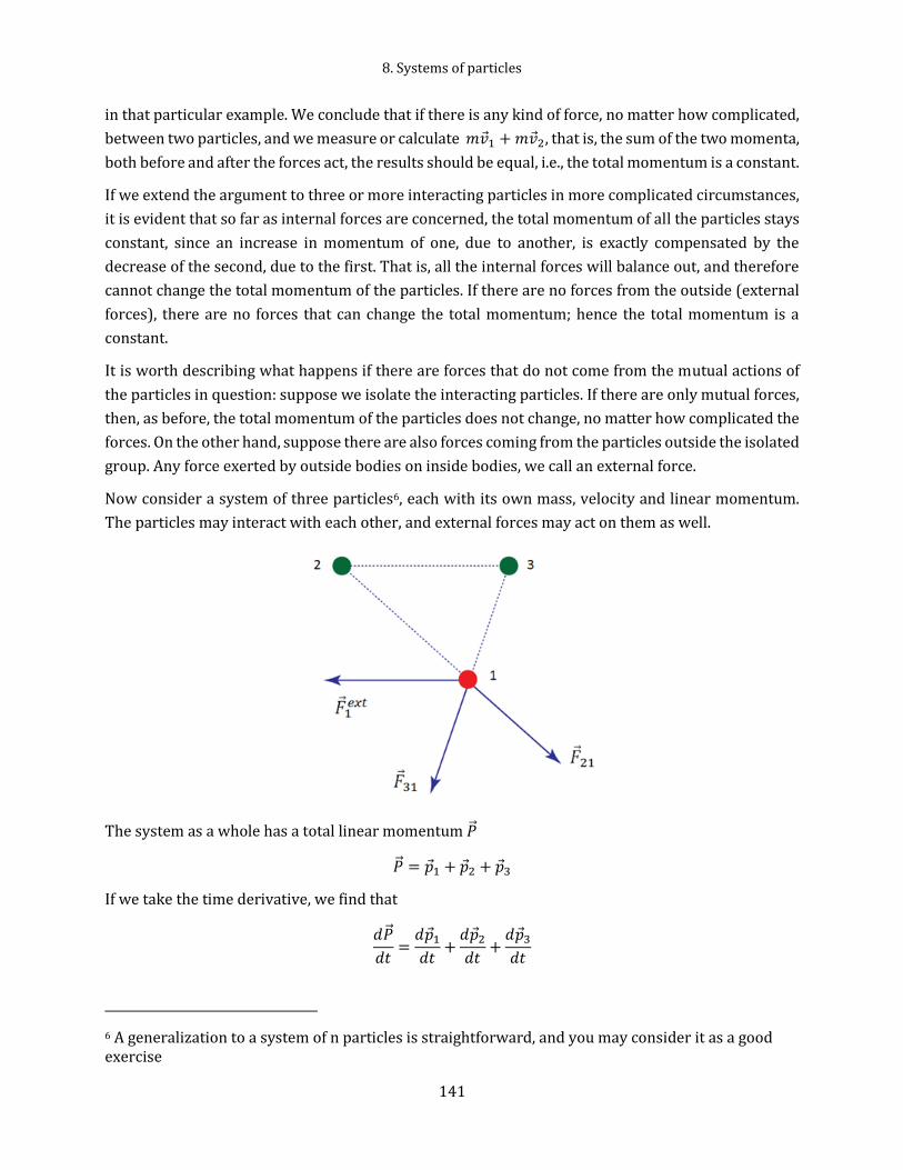
8. Systems of particles
141
in that particular example. We conclude that if there is any kind of force, no matter how complicated,
between two particles, and we measure or calculate 𝑚�⃗�1 + 𝑚�⃗�2, that is, the sum of the two momenta,
both before and after the forces act, the results should be equal, i.e., the total momentum is a constant.
If we extend the argument to three or more interacting particles in more complicated circumstances,
it is evident that so far as internal forces are concerned, the total momentum of all the particles stays
constant, since an increase in momentum of one, due to another, is exactly compensated by the
decrease of the second, due to the first. That is, all the internal forces will balance out, and therefore
cannot change the total momentum of the particles. If there are no forces from the outside (external
forces), there are no forces that can change the total momentum; hence the total momentum is a
constant.
It is worth describing what happens if there are forces that do not come from the mutual actions of
the particles in question: suppose we isolate the interacting particles. If there are only mutual forces,
then, as before, the total momentum of the particles does not change, no matter how complicated the
forces. On the other hand, suppose there are also forces coming from the particles outside the isolated
group. Any force exerted by outside bodies on inside bodies, we call an external force.
Now consider a system of three particles6, each with its own mass, velocity and linear momentum.
The particles may interact with each other, and external forces may act on them as well.
The system as a whole has a total linear momentum �⃗⃗�
�⃗⃗� = 𝑝1 + 𝑝2 + 𝑝3
If we take the time derivative, we find that
𝑑�⃗⃗�
𝑑𝑡=
𝑑𝑝1
𝑑𝑡+
𝑑𝑝2
𝑑𝑡+
𝑑𝑝3
𝑑𝑡
6 A generalization to a system of n particles is straightforward, and you may consider it as a good exercise
8.3 Newton’s second law for a system of particles
142
For every particle
𝑑𝑝𝑖
𝑑𝑡= �⃗�𝑖
𝑒𝑥𝑡 + ∑ �⃗�𝑗𝑖
3
𝑗≠𝑖
Then
𝑑�⃗⃗�
𝑑𝑡= �⃗�1
𝑒𝑥𝑡 + �⃗�21 + �⃗�31 + �⃗�2𝑒𝑥𝑡 + �⃗�12 + �⃗�32 + �⃗�3
𝑒𝑥𝑡 + �⃗�13 + �⃗�23
According to Newton’s third law (action-reaction)
�⃗�21 = −�⃗�12, �⃗�31 = −�⃗�13, �⃗�32 = −�⃗�23
and
𝑑�⃗⃗�
𝑑𝑡= �⃗�1
𝑒𝑥𝑡 + �⃗�2𝑒𝑥𝑡 + �⃗�3
𝑒𝑥𝑡 = �⃗�𝑒𝑥𝑡
where �⃗�𝑒𝑥𝑡 is the net external force, and if �⃗�𝑒𝑥𝑡 = 0 then
𝑑�⃗⃗�
𝑑𝑡= 0 ⇒ �⃗⃗� = 𝑐𝑜𝑛𝑠𝑡 (8.3)
momentum of the entire system of particles is conserved.
This is one of the most important results in classical (Newtonian) mechanics.
Note that momentum of a single particle is not necessarily conserved, only the total momentum of a
closed system.
8.3 Newton’s second law for a system of particles
For a system of point-like particles (see above).
𝑑�⃗⃗�
𝑑𝑡= �⃗�𝑒𝑥𝑡 (8.5)
At this point we introduce the center of mass for a system of n particles
�⃗⃗�𝐶𝑀 =1
𝑀∑ 𝑚𝑖𝑟𝑖
𝑛
𝑖=1
(8.6)
Principle of Conservation of Linear Momentum
If the net force �⃗�𝑒𝑥𝑡 on an N-particle system is zero, the system’s total mechanical momentum
�⃗⃗� = 𝑚1�⃗�1 + 𝑚2�⃗�2 + ⋯ + 𝑚𝑁�⃗�𝑁 (8.4)
is constant

8. Systems of particles
143
where
𝑀 = 𝑚1 + 𝑚2 + ⋯ 𝑚𝑛 = ∑ 𝑚𝑖
𝑛
𝑖=1
(8.7)
is the total mass of the system.
If the particles are distributed in three dimensions, the center of mas can be identified by three
coordinates
𝑥𝐶𝑀 =1
𝑀∑ 𝑚𝑖𝑥𝑖
𝑛
𝑖=1
, 𝑦𝐶𝑀 =1
𝑀∑ 𝑚𝑖𝑦𝑖
𝑛
𝑖=1
, 𝑧𝐶𝑀 =1
𝑀∑ 𝑚𝑖𝑧𝑖
𝑛
𝑖=1
. (8.8)
An ordinary object contains so many particles (atoms) that we can treat it as a continuous distribution
of matter. Then the sums above become integrals.
In this chapter we deal with particle-like systems or simple enough symmetrical objects when the
position of the center of mass is known, e.g. the center of mass of a uniform rod of length L is at L/2
the center of mass of a uniform spherical ball is at the center of the ball.
Differentiating the definition for the center of mass with respect to time gives
�⃗�𝐶𝑀 =1
𝑀∑ 𝑚𝑖�⃗�𝑖
𝑛
𝑖=1
(8.9)
where �⃗�𝑖 is the velocity of the 𝑖 − th particle and �⃗�𝐶𝑀 is the velocity of the center of mass.
Differentiating the last equation with respect to time gives
�⃗�𝐶𝑀 =1
𝑀∑ 𝑚𝑖�⃗�𝑖
𝑛
𝑖=1
=1
𝑀∑ �⃗�𝑖
𝑛
𝑖=1
=1
𝑀�⃗�𝑒𝑥𝑡.
or
𝑀𝑎𝐶𝑀 = �⃗�𝑒𝑥𝑡 (8.10)
Thus the center of mass of a system moves as though all of the mass were concentrated there and all
external forces were applied there.
There are two obvious results from this equation.
If the net force acting on a system is zero, then a system moves with constant velocity
�⃗�𝐶𝑀 = 𝑐𝑜𝑛𝑡𝑎𝑛𝑡 for �⃗�𝑒𝑥𝑡 = 0
And if the center of mass of a system was not moving �⃗�𝐶𝑀 = 0, then the position of the center
of mass �⃗⃗�𝐶𝑀 does not change despite individual positions of particles may change.
�⃗⃗�𝐶𝑀 = 𝑐𝑜𝑛𝑠𝑡𝑎𝑛𝑡 for �⃗�𝐶𝑀 = 0 (if �⃗�𝑒𝑥𝑡 = 0)

8.4 Impulse and Linear Momentum
144
8.4 Impulse and Linear Momentum
Using Newton’s second law in momentum form
�⃗� =𝑑𝑝
𝑑𝑡
we can write
𝑑𝑝 = �⃗�(𝑡)𝑑𝑡
in which �⃗�(𝑡) is a time-varying force. Let’s integrate this equation over the time interval Δ𝑡 from an
initial time 𝑡𝑖 to a final time 𝑡𝑓 . We obtain
∫ 𝑑𝑝�⃗�𝑓
�⃗�𝑖
= ∫ �⃗�(𝑡)𝑑𝑡𝑡𝑓
𝑡𝑖
The left side of the equation is 𝑝𝑓 − 𝑝𝑖 the change in linear momentum of an object. The right side,
which measures both the strength and the duration of the force, is called the impulse 𝐽.
𝐽 = 𝑝𝑓 − 𝑝𝑖 = ∫ �⃗�(𝑡)𝑑𝑡𝑡𝑓
𝑡𝑖
. (8.11)
The last equation can be written in component form as
𝑝𝑓𝑥 − 𝑝𝑖𝑥 = 𝐽𝑥 = ∫ 𝐹𝑥(𝑡)𝑑𝑡𝑡𝑓
𝑡𝑖
, 𝑝𝑓𝑦 − 𝑝𝑖𝑦 = 𝐽𝑦 = ∫ 𝐹𝑦(𝑡)𝑑𝑡𝑡𝑓
𝑡𝑖
, 𝑝𝑓𝑧 − 𝑝𝑖𝑧 = 𝐽𝑧 = ∫ 𝐹𝑧(𝑡)𝑑𝑡𝑡𝑓
𝑡𝑖
.
If 𝐹𝑎𝑣𝑔 is the average magnitude of the force, we can write the magnitude of the impulse for every
component as
𝐽 = 𝑝𝑓 − 𝑝𝑖 = 𝐹𝑎𝑣𝑔Δ𝑡. (8.12)
where Δ𝑡 is the duration of the action of the force.
The SI units for impulse are [Ns]=[kgm/s], which are the same units as momentum.
8.5 Collisions
A collision is an isolated event in which two or more bodies exert relatively strong forces on each
other for a relatively short period of time.
“relatively strong forces” – comparing to external forces
“relatively short period of time” – so that external force produces negligible impulse (change
in momentum)
Let’s consider a system of two colliding bodies. If there to be a collision, then one of the bodies must
be moving, so that the system has a certain kinetic energy and a certain linear momentum before the
collision. During the collision, the kinetic energy and linear momentum of each body are changed by

8. Systems of particles
145
the force from the other body. In this section the discussion is limited to collisions in system that are
closed (no mass enters or leaves them) and isolated (no net external forces act on the bodies within
the system).
Kinetic energy and two types of collisions
Elastic collisions – if the total kinetic energy of the system is unchanged by the collisions (the
kinetic energy of the system is conserved).
This type of collisions is very unlikely in everyday life7, but more common for collisions of
atomic or nuclear particles.
Inelastic collisions – where the kinetic energy of the system is not conserved.
There is a special kind of inelastic collisions called completely inelastic collision if two bodies
stick together after the collision and move as a single object.
Regardless of the forces acting between bodies during the collision, and regardless to what happens
to the total kinetic energy of the system, the total linear momentum is always conserved. That is quite
interesting, namely we can relate momenta before and after a collision even if we do not know details
of the forces during the collision.
8.5.1 Inelastic collision in one dimension
We can write the law of conservation of linear momentum for a two-body system as
𝑝1𝑖 + 𝑝2𝑖 = 𝑝1𝑓 + 𝑝2𝑓
Figure shows two bodies just before and just after they have a one-dimensional collision.
7 In some situations we can approximate a collision of common bodies as elastic - for example a dropping a Superball (also known as a bouncy ball) on a hard floor.
In a closed isolated system, the linear momentum of each colliding body may change but the total
linear momentum �⃗⃗� = 𝑚�⃗�1 + 𝑚�⃗�2 of the system cannot change, whether the collision is elastic or
inelastic.

8.5 Collisions
146
Because the motion is one-dimensional, we can drop the overall arrows for vectors and use only
components along the axis. Then, using 𝑝 = 𝑚𝑣 we can write
𝑚1𝑣1𝑖 + 𝑚2𝑣2𝑖 = 𝑚1𝑣1𝑓 + 𝑚2𝑣2𝑓 (8.13)
Since there is only one equation, we may have only one unknown.
Now let’s consider a completely inelastic collision (after the collision the bodies stick together moving
with the same velocity)
𝑚1𝑣1𝑖 + 𝑚2𝑣2𝑖 = (𝑚1 + 𝑚2)𝑣𝑓
then the final velocity of the combined body
𝑣𝑓 =𝑚1𝑣1𝑖 + 𝑚2𝑣2𝑖
𝑚1 + 𝑚2 (8.14)
The last equation last equation can be analyzed for various masses 𝑚1 and 𝑚2. We will do that for
𝑣2𝑖 = 0 (or the body with mass 𝑚2 happens to be initially at rest)
𝑣𝑓 =𝑚1
𝑚1 + 𝑚2𝑣1𝑖 (8.15)
We note that the combined system moves in the same direction as initially moving body.
Let’s consider three combinations of masses
A massive target: 𝑚1 ≪ 𝑚2 then 𝑣𝑓 ≈ 0 i.e., the combined system is moving with very small
velocity.
A massive projectile: 𝑚1 ≫ 𝑚2 then 𝑣𝑓 ≈ 𝑣1𝑖 i.e., the combined system is moving with
velocity very close to the velocity of the initially moving body.
Equal masses: 𝑚1 = 𝑚2 then 𝑣𝑓 = 𝑣1𝑖/2 i.e., the combined system moves with the final
velocity that is half of the initial velocity.
8.5.2 Elastic collision in one dimension
In an elastic collision, the kinetic energy of each colliding body may change, but the total kinetic
energy of the system does not change.
𝑚1𝑣1𝑖 + 𝑚2𝑣2𝑖 = 𝑚1𝑣1𝑓 + 𝑚2𝑣2𝑓 𝑐𝑜𝑛𝑠𝑒𝑟𝑣𝑎𝑡𝑖𝑜𝑛 𝑜𝑓 𝑙𝑖𝑛𝑒𝑟𝑎 𝑚𝑜𝑚𝑒𝑛𝑡𝑢𝑚 1
2𝑚1𝑣1𝑖
2 +1
2𝑚2𝑣2𝑖
2 =1
2𝑚1𝑣1𝑓
2 +1
2𝑚2𝑣2𝑓
2 𝑐𝑜𝑛𝑠𝑒𝑟𝑣𝑎𝑡𝑖𝑜𝑛 𝑜𝑓 𝑘𝑖𝑛𝑒𝑡𝑖𝑐 𝑒𝑛𝑒𝑟𝑔𝑦 (8.16)
These two equations describe elastic collision of two bodies in one dimension. Having two equations
we can solve the system for two unknowns. If we know the masses and initial velocities, then we can
solve these equations for the velocities after the collision 𝑣1𝑓 and 𝑣2𝑓.We rewrite the momentum
equations as
𝑚1(𝑣1𝑖 − 𝑣1𝑓) = 𝑚2(𝑣2𝑓 − 𝑣2𝑖) (8.17)
and the kinetic energy equation can be rewritten as

8. Systems of particles
147
𝑚1(𝑣1𝑖2 − 𝑣1𝑓
2 ) = 𝑚2(𝑣2𝑓2 − 𝑣2𝑖
2 )
noting that (𝑎2 − 𝑏2) = (𝑎 − 𝑏)(𝑎 + 𝑏) we rewrite the last equation
𝑚1(𝑣1𝑖 − 𝑣1𝑓)(𝑣1𝑖 + 𝑣1𝑓) = 𝑚2(𝑣2𝑓 − 𝑣2𝑖)(𝑣2𝑓 + 𝑣2𝑖) (8.18)
Dividing the left and the right sides of the last equation (8.18) by the corresponding sides of the linear
momentum equation (8.17) gives
𝑣1𝑖 + 𝑣1𝑓 = 𝑣2𝑓 + 𝑣2𝑖 𝑜𝑟 𝑣1𝑖 − 𝑣2𝑖 = 𝑣2𝑓 − 𝑣1𝑓
The results tells us that for one dimensional elastic head-on collisions, the relative speed of the two
objects after the collisions has the same magnitude as before (but opposite direction), no matter what
the masses are.
From the last equation,
𝑣2𝑓 = 𝑣1𝑖 − 𝑣2𝑖 + 𝑣1𝑓
Substituting this result into (8.17) gives
𝑚1(𝑣1𝑖 − 𝑣1𝑓) = 𝑚2(𝑣1𝑖 − 𝑣2𝑖 + 𝑣1𝑓 − 𝑣2𝑖) 𝑜𝑟 (𝑚1 − 𝑚2)𝑣1𝑖 + 2𝑚2𝑣2𝑖 = (𝑚1 + 𝑚2)𝑣1𝑓
Solving for 𝑣1𝑓
𝑣1𝑓 =𝑚1 − 𝑚2
𝑚1 + 𝑚2𝑣1𝑖 +
2𝑚2
𝑚1 + 𝑚2𝑣2𝑖 (8.19)
Having 𝑣1𝑓 we can easily (simply algebra) find 𝑣2𝑓 from (8.17).
𝑣2𝑓 =2𝑚1
𝑚1 + 𝑚2𝑣1𝑖 +
𝑚2 − 𝑚1
𝑚1 + 𝑚2𝑣2𝑖 (8.20)
These equations express the final velocities in terms of initial velocities.
Let us look at a few special situations. For clarity of our analysis we assume that a projectile body 𝑚1
moves toward a target body 𝑚2 that is initially at rest 𝑣2𝑖 = 0. Then
𝑣1𝑓 =𝑚1 − 𝑚2
𝑚1 + 𝑚2𝑣1𝑖 (8.21)
𝑣2𝑓 =2𝑚1
𝑚1 + 𝑚2𝑣1𝑖 (8.22)
Equal masses: If 𝑚1 = 𝑚2 then
𝑣1𝑓 = 0 𝑎𝑛𝑑 𝑣2𝑓 = 𝑣1𝑖
which we may call a pool player result. It predicts that after a head-on collision of bodies with
equal masses, body 1 (initially moving) stops dead and body 2 (initially at rest) takes off with
the initial speed of body 1.
A massive target: A massive target means that 𝑚2 ≫ 𝑚1 (for example firing a golf ball into a
cannonball. Then
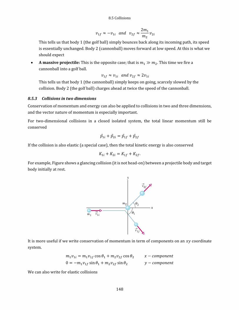
8.5 Collisions
148
𝑣1𝑓 ≈ −𝑣1𝑖 𝑎𝑛𝑑 𝑣2𝑓 ≈2𝑚1
𝑚2𝑣2𝑖
This tells us that body 1 (the golf ball) simply bounces back along its incoming path, its speed
is essentially unchanged. Body 2 (cannonball) moves forward at low speed. At this is what we
should expect
A massive projectile: This is the opposite case; that is 𝑚1 ≫ 𝑚2. This time we fire a
cannonball into a golf ball.
𝑣1𝑓 ≈ 𝑣1𝑖 𝑎𝑛𝑑 𝑣2𝑓 ≈ 2𝑣1𝑖
This tells us that body 1 (the cannonball) simply keeps on going, scarcely slowed by the
collision. Body 2 (the golf ball) charges ahead at twice the speed of the cannonball.
8.5.3 Collisions in two dimensions
Conservation of momentum and energy can also be applied to collisions in two and three dimensions,
and the vector nature of momentum is especially important.
For two-dimensional collisions in a closed isolated system, the total linear momentum still be
conserved
𝑝1𝑖 + 𝑝2𝑖 = 𝑝1𝑓 + 𝑝2𝑓
If the collision is also elastic (a special case), then the total kinetic energy is also conserved
𝐾1𝑖 + 𝐾2𝑖 = 𝐾1𝑓 + 𝐾2𝑓 .
For example, Figure shows a glancing collision (it is not head-on) between a projectile body and target
body initially at rest.
It is more useful if we write conservation of momentum in term of components on an 𝑥𝑦 coordinate
system.
𝑚1𝑣1𝑖 = 𝑚1𝑣1𝑓 cos 𝜃1 + 𝑚2𝑣2𝑓 cos 𝜃2 𝑥 − 𝑐𝑜𝑚𝑝𝑜𝑛𝑒𝑛𝑡
0 = −𝑚1𝑣1𝑓 sin 𝜃1 + 𝑚2𝑣2𝑓 sin 𝜃2 𝑦 − 𝑐𝑜𝑚𝑝𝑜𝑛𝑒𝑛𝑡
We can also write for elastic collisions

8. Systems of particles
149
1
2𝑚1𝑣1𝑖
2 =1
2𝑚1𝑣1𝑓
2 +1
2𝑚2𝑣2𝑓
2
These three equations have seven variables: two masses, three speeds and two angles. If we know
any four of these quantities, we can solve the three equations for the remaining three quantities.
8.6 The center of mass of solid bodies*
Calculating the center of mass for a solid object is rather more complicated exercise than finding the
center of mass of a system of point-like particles. However, we apply the same basic idea thinking
about a solid object as a system containing a large number of particles with continuous mass
distribution. Let’s divide the object into elements of mass Δ𝑚𝑖 with coordinates 𝑥𝑖 , 𝑦𝑖 , 𝑧𝑖. Then, the 𝑥
coordinate of the center of mass is approximately
𝑥𝐶𝑀 ≈∑ 𝑥𝑖Δ𝑚𝑖𝑖
𝑀
Using calculus we can write exactly
𝑥𝐶𝑀 = limΔ𝑚𝑖→0
∑ 𝑥𝑖Δ𝑚𝑖𝑖
𝑀=
1
𝑀∫ 𝑥𝑑𝑚 (8.23)
where 𝑑𝑚 is the element of mass and the integral is taken over the extent of the object. The total mass
is given simply by
𝑀 = ∫ 𝑑𝑚
Likewise we can define 𝑦𝐶𝑀 and 𝑧𝐶𝑀.
For a solid three-dimensional body the element of mass is just 𝑑𝑚 = 𝜌𝑑𝑉, where 𝑑𝑉 is the element of
volume, and 𝜌 is the density (that can be variable, namely 𝜌(𝑥, 𝑦, 𝑧). For a laminar body (i.e. a uniform
sheet of material) the element of mass is 𝑑𝑚 = 𝜎𝑑𝐴, where 𝜎(𝑥, 𝑦) is the mass per unit area of the
body, and 𝑑𝐴 is an area element. Finally, for a body in the form of a thin wire we have 𝑑𝑚 = 𝜆 𝑑𝑠,
where 𝜆 is the mass per unit length and 𝑑𝑠 is an element of arc length along the wire.
Let’s find the center of mass of a rod of length 𝐿 that has a uniform density 𝜆. The total mass of the rod
is
𝑀 = ∫ 𝜆𝑑𝑥𝐿
0
= 𝜆𝐿
and the center of mass is located at
𝑥𝐶𝑀 =1
𝑀∫ 𝑥𝜆𝑑𝑥
𝐿
0
=1
𝜆𝐿
𝜆𝐿2
2=
𝐿
2.
Two- and three- dimensional cases require evaluation of multiple integrals. Such integration goes
beyond this course.

8.7 Dynamics of Bodies of Variable Mass; Rocket propulsion
150
8.7 Dynamics of Bodies of Variable Mass; Rocket propulsion
Conservation of linear momentum is the foundation for the motion in space (where there is no any
gas atmosphere).
Consider a rocket with mass 𝑀 travelling in the positive 𝑥 direction with speed 𝑣. Instead of using
notation 𝑣𝑥 for components we will write just 𝑣. The thrust of the rocket engine is created by ejecting
the fuel combustion products in a direction opposite to the motion of the rocket with the exhaust
speed 𝑣𝑒𝑥 relative to the rocket. Since the rocket is ejecting mass, its mass 𝑀 is decreasing.
At time 𝑡, the linear momentum is 𝑚𝑣, while at time 𝑡 + 𝑑𝑡 the rocket mass is (𝑚 + 𝑑𝑚), where 𝑑𝑚 is
negative, and its momentum is (𝑚 + 𝑑𝑚)(𝑣 + 𝑑𝑣). The ejected fuel at that time has mass – 𝑑𝑚 and
velocity (𝑣 − 𝑣𝑒𝑥) relative to the ground. Then the total momentum at time 𝑡 + 𝑑𝑡 is
𝑝(𝑡 + 𝑑𝑡) = (𝑚 + 𝑑𝑚)(𝑣 + 𝑑𝑣) − 𝑑𝑚(𝑣 − 𝑣𝑒𝑥) = 𝑚𝑣 + 𝑚𝑑𝑣 + 𝑑𝑚 𝑣𝑒𝑥
where we neglected the small term 𝑑𝑚 𝑑𝑣 (an infinitesimal of the second order). Thus, the change in
the total momentum is
𝑑𝑝 = 𝑝(𝑡 + 𝑑𝑡) − 𝑝(𝑡) = 𝑚 𝑑𝑣 + 𝑑𝑚 𝑣𝑒𝑥
If there is an external force 𝐹𝑒𝑥𝑡 acting on the rocket, then the change of momentum is 𝐹𝑒𝑥𝑡𝑑𝑡. Without
an external force the linear momentum is conserved and 𝑑𝑝 = 0. Therefore
𝑚 𝑑𝑣 = −𝑑𝑚 𝑣𝑒𝑥 (8.24)
or with dime derivatives we get
𝑚𝑑𝑣
𝑑𝑡= −𝑣𝑒𝑥
𝑑𝑚
𝑑𝑡 (8.25)
where 𝑑𝑚 𝑑𝑡⁄ is the rate at which the rocket is ejecting mass. This equation describes the motion of
rockets in the absence of external forces.
Equation (8.25) looks just like Newton’s second law where the term on the right is called the thrust:
𝐹𝑡ℎ𝑟𝑢𝑠𝑡 = −𝑣𝑒𝑥
𝑑𝑚
𝑑𝑡
This force is positive since 𝑑𝑚 𝑑𝑡⁄ is negative.
Equation (8.24) can be solved using separation of variables (we assume that the exhaust speed is
constant)
𝑑𝑣 = −𝑣𝑒𝑥
𝑑𝑚
𝑚

8. Systems of particles
151
Assuming that at 𝑡 = 0 the mass of the rocket was 𝑚0 and the initial velocity 𝑣0 and integrating both
sides
∫ 𝑑𝑣𝑣
𝑣0
= −𝑣𝑒𝑥 ∫𝑑𝑚
𝑚
𝑀
𝑀0
we easily get
𝑣 − 𝑣0 = 𝑣𝑒𝑥 ln𝑚0
𝑚
or
𝑣(𝑡) = 𝑣0 + 𝑣𝑒𝑥 ln𝑚0
𝑚
where 𝑚 rocket’s mass at any time. Thus equation describes the change in the velocity of the rocket
when its mass changes from 𝑚0 to 𝑚. If the engine is applied to slow down the motion then we replace
𝑣𝑒𝑥 on −𝑣𝑒𝑥.
Let us quickly evaluate efficiency of delivering a payload to a low orbit around Earth. Assuming the
initial speed 𝑣0 = 0 𝑚/𝑠, the final speed 8 𝑘𝑚/𝑠, the exhaust speed 4 𝑘𝑚/𝑠, and neglecting the force
of gravity (too optimistic assumption) we get for the original mass 𝑚0 to be about 90% of fuel.
A crude estimation for flying to Mars and come back gives for a payload about 1/1500 of the starting
mass.
8.8 Examples
Example 8-1
A marksman holds a rifle of mass 𝑚𝑅 = 3.0 𝑘𝑔 loosely in his hands, so as to let it recoil freely when
fired. He fires a bullet of mass 𝑚𝐵 = 5.0 𝑔 horizontally with a velocity relative to the ground of 𝑣𝐵 =
300 𝑚 𝑠⁄ . What is the recoil velocity of the rifle? What is the kinetic energy of the bullet? Of the rifle?
SOLUTION:
1. Physics – conservation of linear momentum for the closed isolated system. We may assume the net
external force from the marksman as zero while the bullet moves inside the barrel.
2. The basic equation
𝑚1�⃗�1 + 𝑚2�⃗�2 = 𝑐𝑜𝑛𝑠𝑡𝑎𝑛𝑡
or
𝑚1𝑣1𝑖 + 𝑚2𝑣2𝑖 = 𝑚1𝑣1𝑓 + 𝑚2𝑣2𝑓
3. Initially the rifle and bullet were not moving 𝑣𝐵𝑖 = 0, 𝑣𝑅𝑖 = 0 then for our one-dimensional case
0 = 𝑚𝐵𝑣𝐵𝑓 + 𝑚𝑅𝑣𝑅𝑓

8.8 Examples
152
4. Solving for 𝑣𝑅𝑓
𝑣𝑅𝑓 = −𝑚𝐵
𝑚𝑅𝑣𝐵𝑓
For kinetic energies (we only need the definition, there is no conservation of energy)
𝐾𝐵 =1
2𝑚𝐵𝑣𝐵𝑓
2 𝐾𝑅 =1
2𝑚𝑅𝑣𝑅𝑓
2
5. Calculations
𝑣𝑅𝑓 = −0.005 𝑘𝑔
3.0 𝑘𝑔300 𝑚 𝑠⁄ = −0.500 𝑚 𝑠⁄
𝐾𝐵 =1
20.005 𝑘𝑔 ∙ (300 𝑚 𝑠⁄ )2 = 225 𝐽
𝐾𝑅 =1
23.0 𝑘𝑔 ∙ (−0.5 𝑚 𝑠⁄ )2 = 0.375 𝐽
6. Looking back.
Units are correct. The recoil speed looks as a true one. It is interesting to note that while the bullet
and rifle have the same magnitude of the final momenta; their kinetic energies are quite different
because of large difference in speeds.
To satisfy our curiosity, let us derive the ratio of kinetic energy of the rifle to bullet
𝐾𝑅
𝐾𝐵=
12 𝑚𝑅𝑣𝑅𝑓
2
12
𝑚𝐵𝑣𝐵𝑓2
=𝑚𝑅 (
𝑚𝐵𝑚𝑅
𝑣𝐵𝑓)2
𝑚𝐵𝑣𝐵𝑓2 =
𝑚𝐵
𝑚𝑅
Thus the heavier the rifle, the less kinetic energy is transferred to it.
Example 8-2
A heavy wooden crate rests on a floor. A bullet is fired horizontally into the crate so that the bullet
stopping in it. How far will the block slide before coming to a stop? The mass of the bullet is 16.0 g,
the mass of the block is 70.0 kg, the bullet’s impact speed is 300 m/s and the coefficient of kinetic
friction between the crate and the wooden floor is 0.22. (Assume that the bullet does not cause the
crate to spin.)
SOLUTION:
1. Physics – a) conservation of linear momentum for the closed isolated system (assuming we may
disregard any external forces while the bullet penetrates the crate), b) conservation of energy after
the collision).
2. The basic equation:
for the collision (note that the energy is NOT conserved during the inelastic collision)

8. Systems of particles
153
𝑚1𝑣1𝑖 + 𝑚2𝑣2𝑖 = 𝑚1𝑣1𝑓 + 𝑚2𝑣2𝑓
and after the collision
1
2(𝑚1 + 𝑚2)𝑣𝑓
2 = 𝜇𝑘(𝑚1 + 𝑚2)𝑔𝑥
3. Initially the crate was not moving 𝑣2𝑖 = 0, but then the system “bullet + crate” moves as a whole
𝑚1𝑣1𝑖 = (𝑚1 + 𝑚2)𝑣𝑓
and for the stopping 𝑥 distance we apply conservation of energy
1
2(𝑚1 + 𝑚2)𝑣𝑓
2 = 𝜇𝑘(𝑚1 + 𝑚2)𝑔𝑥
4. Solving first for 𝑣𝑓
𝑣𝑓 =𝑚1
𝑚1 + 𝑚2𝑣1𝑖
then using conservation of energy gives
𝑥 =𝑣𝑓
2
2𝜇𝑘𝑔=
1
2𝜇𝑘𝑔(
𝑚1
𝑚1 + 𝑚2)
2
𝑣1𝑖2
5. Calculations
𝑥 = 0.00109 𝑚 ≈ 0.1 𝑐𝑚
6. Looking back.
The dimension of 𝑥 is correct (meters). The stopping distance is small (less than half an inch) but
reasonable. It is interesting to note that Hollywood movies are so wrong when an object (a body) flies
far away with high speed after being hit by a bullet. (See Mythbusters, season 2005, episode 25. Myths
tested: Can a person be blown away by a bullet?)
Example 8-3
You have been called to testify in a trial involving a head-on collision. Car A weighs 1500 lb and was
traveling eastward with an initial speed of 𝑣𝐴. Car B weighs 1100 lb and was traveling westward at
an initial speed of 𝑣𝐵 = 45 𝑚𝑝ℎ. The cars locked bumpers and slid eastward with their wheels locked
for 19 ft before stopping. The coefficient of kinetic friction between the tires and the road was
measured to be 𝜇𝑘 = 0.75.
How fast (in mph) was car A travelling just before the collision? (note – English units are used in U.S.
legal proceedings.)
SOLUTION:

8.8 Examples
154
1. Physics – completely inelastic collision + dissipation of kinetic energy through friction
(conservation of energy). (This example is somewhat similar to example 9-2.)
2. The basic equations
𝑚𝐴𝑣𝐴 + 𝑚𝐵𝑣𝐵 = (𝑚𝐴 + 𝑚𝐵)𝑣𝑓 completely inelastic collision
1
2(𝑚𝐴 + 𝑚𝐵)𝑣𝑓
2 = 𝜇𝑘(𝑚𝐴 + 𝑚𝐵)𝑔𝑥 conservation of energy (after)
3. Assume that car A was moving in the positive 𝑥-direction (eastward), and then the direction of card
B was negative (westward) (keeping correct signs is important!)
𝑚𝐴𝑣𝐴 − 𝑚𝐵𝑣𝐵 = (𝑚𝐴 + 𝑚𝐵)𝑣𝑓
4. From conservation of energy we can easily find the final speed of the wreckage
𝑣𝑓 = √2𝜇𝑘𝑔𝑥
Using it in the momentum equation
𝑣𝐴 =𝑚𝐵
𝑚𝐴𝑣𝐵 +
𝑚𝐴 + 𝑚𝐵
𝑚𝐴√2𝜇𝑘𝑔𝑥
5. Calculations
First we need to switch to SI units for speed and distance, but we can keep English units for masses
since they are entering equation as ratios.
45 𝑚𝑝ℎ = 45 𝑚𝑖𝑙𝑒
ℎ (
1609 𝑚
1 𝑚𝑖𝑙𝑒) (
1 ℎ
3600 𝑠) = 20 𝑚/𝑠
19 𝑓𝑡 = 19 𝑓𝑡 1.0 𝑚
3.28 𝑓𝑡= 5.8 𝑚
𝑣𝐴 =1100 𝑙𝑏
1500 𝑙𝑏20 𝑚 𝑠⁄ +
1100 𝑙𝑏 + 1500𝑙𝑏
1500 𝑙𝑏√2 ∙ 0.75 ∙ 9.8 𝑚 𝑠2⁄ ∙ 5.8 𝑚 = 30.7 𝑚 𝑠⁄ ,
30.7 𝑚 𝑠⁄ = 30.7𝑚
𝑠(
1 𝑚𝑖𝑙𝑒
1609 𝑚) (
3600 𝑠
1 ℎ) = 69 𝑚𝑝ℎ
6. Looking back.
Units are correct. If the wreckage slides eastward, and the masses or the cars are comparable, then
car A must have been traveling faster than car B when they collided. It corresponds to our result.
Example 8-4
It is well known that bullets and other missiles fired at Superman simply bounce off his chest. Suppose
that a gangster sprays Superman’s chest with 5.0 g bullets at a rate of 100 bullets/min, and the speed
of each bullet is 500 m/s. Suppose too that the bullets rebound straight back with no change speed.
What is the magnitude of the average force on Superman’s chest from the stream of bullets?

8. Systems of particles
155
SOLUTION:
1. Physics –force, momentum.
2. The basic equation
The force can be found from the impulse (change of momentum)
𝐽 = 𝑝𝑓 − 𝑝𝑖 = 𝐹𝑎𝑣𝑔Δ𝑡.
3. Assume that bullets were incoming from positive 𝑥 direction (or negative initial velocity)
𝑚𝑣0 + 𝑚𝑣0 = 𝐹𝑎𝑣𝑔Δ𝑡.
or
2𝑚𝑣0 = 𝐹𝑎𝑣𝑔Δ𝑡
4. Solving the last equation for 𝐹𝑎𝑣𝑔
𝐹𝑎𝑣𝑔 =2𝑚𝑣0
Δ𝑡
5. Calculations
𝐹𝑎𝑣𝑔 =2 ∙ 0.005 𝑘𝑔 ∙ 100 ∙ 500 𝑚 𝑠⁄
60 𝑠= 8.3 𝑁
6. Looking back.
Units are correct. Commons sense cannot be applied to Superman, but the force (8.3 N or about 2 lb)
looks reasonable and small (unlike in movies!)
Example 8-5
The ballistic pendulum was used to measure the speeds of bullets before electronic timing devices
were developed. The version is shown in Figure consists of a large block of wood of mass M=5.4 kg,
hanging from two long cords. A bullet of mass 9.5 g is fired into the block, coming quickly to rest. The
block + bullet then swing upward, their center of mass rising a vertical distance h=6.3 cm before the
pendulum comes momentarily to rest at the end of its arc.
a) What is the speed of the bullet just prior to the collision?
b) Find the fraction of kinetic energy lost in the ballistic-pendulum collision.
SOLUTION:

8.8 Examples
156
1. Physics – completely inelastic collision + conservation of
mechanical energy.
2. The basic equations
𝑚𝑣𝑖 + 𝑀𝑣𝐵𝑖 = (𝑚 + 𝑀)𝑣𝑓
1
2(𝑚 + 𝑀)𝑣𝑓
2 = (𝑚 + 𝑀)𝑔ℎ
3. Initially the wooden block was not moving 𝑣𝐵𝑖 = 0
𝑚𝑣𝑖 = (𝑚 + 𝑀)𝑣𝑓
4. Solving for 𝑣𝑓
𝑣𝑓 =𝑚
𝑚 + 𝑀𝑣𝑖
Using it in the energy equation
1
2𝑣𝑓
2 = 𝑔ℎ 𝑜𝑟 1
2
𝑚2
(𝑚 + 𝑀)2𝑣𝑖
2 = 𝑔ℎ
then
𝑣𝑖 =𝑚 + 𝑀
𝑚√2𝑔ℎ
Fraction of kinetic energy lost in the collision
𝑅 =𝐾𝑖 − 𝐾𝑓
𝐾𝑖= 1 −
12
(𝑚 + 𝑀)𝑣𝑓2
12 𝑚𝑣𝑖
2= 1 −
𝑚 + 𝑀
𝑚
𝑚2
(𝑚 + 𝑀)2
𝑣𝑖2
𝑣𝑖2 = 1 −
𝑚
𝑚 + 𝑀=
𝑀
𝑚 + 𝑀
5. Calculations
𝑣𝑖 =(0.0095 𝑘𝑔 + 5.4 𝑘𝑔)
0.0095 𝑘𝑔√2 ∙ 9.8 𝑚 𝑠2⁄ ∙ 0.063𝑚 = 630 𝑚 𝑠⁄ , 𝑅 =
5.4 𝑘𝑔
0.0095 𝑘𝑔 + 5.4 𝑘𝑔= 0.998
6. Looking back.
Units are correct. The speed of the bullet matches common speeds for rifles.
Example 8-6
A careless physics professor is in the path of a pack of stampeding elephants when Tarzan swings in
to the rescue on a rope vine, hauling him off to safety. The length of the vine is 16 m, and Tarzan starts
his swing with the rope horizontal. If the professor’s mass is 80 kg and Tarzan’s mass is also 80 kg to
what height above the ground will the pair swing? (Assume the rope is vertical when Tarzan grabs
the professor.)
SOLUTION:
8. Systems of particles
157
1. Physics – completely inelastic collision + conservation of mechanical energy.
2. The basic equations
𝑚1𝑣1𝑖 + 𝑚2𝑣2𝑖 = (𝑚1 + 𝑚2)𝑣𝑓
1
2𝑀𝑣2 = 𝑀𝑔ℎ
3. There are three phases of motion in the problem, namely a) Tarzan swings from the tree
(conservation of mechanical energy), b) picking up the professor (completely inelastic collision), and
c) the pair swings up (conservation of mechanical energy). Assuming that 1 stands for Tarzan and 2
for the professor one can write
𝑚1𝑔𝑅 =1
2𝑚1𝑣1
2 𝑝ℎ𝑎𝑠𝑒 1
𝑚1𝑣1 = (𝑚1 + 𝑚2)𝑣𝑓 𝑝ℎ𝑎𝑠𝑒 2
(𝑚1 + 𝑚2)𝑣𝑓
2
2= (𝑚1 + 𝑚2)𝑔ℎ 𝑝ℎ𝑎𝑠𝑒 3
where 𝑅 is the length of the vine, and ℎ is the height above the ground for Tarzan and the professor.
4. Solving for ℎ (after simple algebra)
ℎ = (𝑚1
𝑚1 + 𝑚2)
2
𝑅
5. Calculations
𝑅 = (80 𝑘𝑔
80 𝑘𝑔 + 80 𝑘𝑔)
2
16 𝑚 = 4 𝑚
6. Looking back.
Units are correct. it is interesting that the final height is one quarter of the rope, not one half as one
would expect using just conservation of energy.
Example 8-7
A 4.5 kg dog stands on an 18 kg flatboat 𝐿 + 𝑑 = 6.1 𝑚 from the shore. The dog walks 𝐿 = 2.4 𝑚 along
the boat toward the shore, and then stops. Assuming there is no friction between the boat and the
water, find how far the dog is then from the shore.
Hint: use a stationary point as a reference point +having a diagram with proper notations helps a lot.
Note that the center of mass for a uniform boat is in the middle (at L/2).

8.8 Examples
158
SOLUTION:
1. Physics: a system of particles (the
dog and boat)
2. The basic equation
𝑀𝑎𝐶𝑀 = �⃗�𝑒𝑥𝑡
3. Let 1 be the dog and 2 be the boat.
We choose the origin at the shore
line.
The net force acting on the system is zero (gravity is balanced by the buoyant force) �⃗�𝑒𝑥𝑡 = 0. Initially
the system was stationary 𝑣𝐶𝑀 = 0, then the position of the center of mass does not change despite
the dog and boat change their positions, or 𝑥𝐶𝑀 = 𝑐𝑜𝑛𝑠𝑡𝑎𝑛𝑡
𝑚1𝑥1𝑖 + 𝑚2𝑥2𝑖
𝑚1 + 𝑚2=
𝑚1𝑥1𝑓 + 𝑚2𝑥2𝑓
𝑚1 + 𝑚2
Using notations from the diagram
𝑚1(𝑑 + 𝐿) + 𝑚2 (𝑑 +𝐿
2) = 𝑚1(𝑑 + 𝑥) + 𝑚2 (𝑑 + 𝑥 +
𝐿
2)
4. Solving the last equation for 𝑥
𝑥 =𝑚1
𝑚1 + 𝑚2𝐿
Note that the answer does not depend on our choice of the origin. It was easier to set the origin at the
initial position of the left side of the boat and adding the distance 𝑑 later.
So, the dog’s position relative to the shore is
𝑑 + 𝑥 = 𝑑 +𝑚1
𝑚1 + 𝑚2𝐿
5. Calculations
Note that 𝑑 = 6.1 𝑚 − 2.4 𝑚 = 3.7 𝑚
𝑑 + 𝑥 = 3.7 𝑚 +4.5 𝑘𝑔
4.5 𝑘𝑔 + 18 𝑘𝑔2.4 𝑚 = 4.18 𝑚
6. Looking back.
Units are correct. The distance is not too short or too large.
For infinitely heavy boat 𝑚2 ≫ 𝑚1 we get 𝑥 ≈ 0 and 𝑑 + 𝑥 = 3.7 𝑚 that corresponds to common
sense.

8. Systems of particles
159
Example 8-8
The cat Tom, of mass 7.0 kg, and the mouse Jerry (see the cartoon "Tom and Jerry") are in a 1.0 kg
canoe. When the canoe is at rest in the placid water, they exchange seats, which are 2.0 m apart and
symmetrically located with respect to the canoe's center. The canoe moves 1.7 m relative to the shore
during the exchange. What is Jerry's mass?
SOLUTION
1. Physics – system of “particles”
(Tom, Jerry, the boat)
2. The basic equation
𝑀𝑎𝐶𝑀 = �⃗�𝑒𝑥𝑡
3. Since there are no external
forces, initially the system was at
rest, and we have one dimensional
case, then
𝑥𝐶𝑀 =1
𝑀∑ 𝑚𝑖𝑥𝑖
𝑛
𝑖=1
= 𝑐𝑜𝑛𝑠𝑡𝑎𝑛𝑡
or despite all the changes the center of mass stays at the same position.
𝑚𝑇𝑥𝑇𝑖 + 𝑚𝐽𝑥𝐽𝑖 + 𝑚𝑏𝑥𝑏𝑖
𝑚𝑇 + 𝑚𝐽 + 𝑚𝑏=
𝑚𝑇𝑥𝑇𝑓 + 𝑚𝐽𝑥𝐽𝑓 + 𝑚𝑏𝑥𝑏𝑓
𝑚𝑇 + 𝑚𝐽 + 𝑚𝑏
Using notations from the diagram, and assuming that the boat has moved to the right
𝑚𝑇0 + 𝑚𝐽𝐿 + 𝑚𝑏
𝐿
2= 𝑚𝑇(𝐿 + 𝑥) + 𝑚𝐽𝑥 + 𝑚𝑏 (
𝐿
2+ 𝑥)
4. Solving the last equation for 𝑚𝐽
𝑚𝐽(𝐿 − 𝑥) = 𝑚𝑇(𝐿 + 𝑥) + 𝑚𝑏𝑥
𝑚𝐽 =𝑚𝑇(𝐿 + 𝑥) + 𝑚𝑏𝑥
𝐿 − 𝑥
5. Calculations
𝑚𝐽 =7 𝑘𝑔(2 𝑚 + 1.7 𝑚) + 1 𝑘𝑔 ∗ 1.7 𝑚
2 𝑚 − 1.7 𝑚= 92 𝑘𝑔
6. Looking back.
Units are correct but the answer does not have sense! We expect Jerry to be less than Tom. It means
that our assumption that the boat has moved to the right was not correct. If Tom was heavier than
Jerry, then the boat had to move to the left. Thus we should rather have negative 𝑥

8.8 Examples
160
𝑚𝐽 =𝑚𝑇(𝐿 − 𝑥) + 𝑚𝑏(−𝑥)
𝐿 + 𝑥
𝑚𝐽 =7 𝑘𝑔(2 𝑚 − 1.7 𝑚) − 1 𝑘𝑔 ∗ 1.7 𝑚
2 𝑚 + 1.7 𝑚= 0.108 𝑘𝑔
Now it looks reasonable.
Example 8-9
At an intersection, a car of mass 1500 kg going east collides with a
pickup truck with mass 1800 kg is travelling north and ran a red light.
The two vehicles stick together as a result of the collision and the
wreckage slides 16.0 meters in a straight line 240 east of north. The
coefficient of kinetic friction for the tires on the road is 0.90.
Calculate the speed of each vehicle before the collision.
SOLUTION:
1. Physics – completely inelastic collision in two dimensions+ dissipation of kinetic energy through
friction (conservation of energy).
2. The basic equations
Completely inelastic collision (in vector form)
𝑚1�⃗�1𝑖 + 𝑚2�⃗�2𝑖 = (𝑚1 + 𝑚2)�⃗�𝑓
Conservation of energy (all kinetic energy after the collision goes into termal/friction)
1
2(𝑚1 + 𝑚2)𝑣𝑓
2 = 𝜇𝑘(𝑚1 + 𝑚2)𝑔𝑑
3. Using components for velocities (where 1 is the car, and 2 is the truck)
𝑥 − 𝑐𝑜𝑚𝑝𝑜𝑛𝑒𝑛𝑡 𝑚1𝑣1𝑖 + 0 = (𝑚1 + 𝑚2)𝑣𝑓 sin 𝜃
𝑦 − 𝑐𝑜𝑚𝑝𝑜𝑛𝑒𝑛𝑡 0 + 𝑚2𝑣2𝑖 = (𝑚1 + 𝑚2)𝑣𝑓 cos 𝜃
4. From conservation of energy we can easily find the final speed of the wreckage
𝑣𝑓 = √2𝜇𝑘𝑔𝑑
Using it in the momentum equation
𝑣1𝑖 =(𝑚1 + 𝑚2)
𝑚1𝑣𝑓 sin 𝜃 =
(𝑚1 + 𝑚2)
𝑚1(√2𝜇𝑘𝑔𝑑) sin 𝜃
𝑣2𝑖 =(𝑚1 + 𝑚2)
𝑚2𝑣𝑓 cos 𝜃 =
(𝑚1 + 𝑚2)
𝑚2(√2𝜇𝑘𝑔𝑑) cos 𝜃
5. Calculations

8. Systems of particles
161
𝑣1𝑖 = 15 𝑚 𝑠⁄ 𝑜𝑟 34 𝑚𝑝ℎ
𝑣2𝑖 = 28 𝑚 𝑠⁄ 𝑜𝑟 63 𝑚𝑝ℎ
6. Looking back.
Units are correct. Both speeds are possible (not too fast or too slow) for cars.
*add example on rocket motion (with gravity)

9.1 Rotational motion
162
9 Rotation in two dimensions
9.1 Rotational motion
In the previous chapters, we have been studying the mechanics of points, or small particles whose
internal structure does not concern us. For the next two chapters we shall study the application of
Newton's laws to more complicated things. When the world becomes more complicated, it also
becomes more interesting, and we shall find that the phenomena associated with the mechanics of a
more complex object than just a point are really quite striking. Of course these phenomena involve
nothing but combinations of Newton's laws, but it is sometimes hard to believe that only �⃗� = 𝑚�⃗� is
at work.
The more complicated objects we deal with can be of several kinds: water flowing, galaxies whirling,
and so on. The simplest "complicated" object to analyze, at the start, is what we call a rigid body, a
solid object that is turning as it moves about. However, even such a simple object may have a most
complex motion, and we shall therefore first consider the simplest aspects of such motion, in which
an extended body rotates about a fixed axis. A given point on such a body then moves in a plane
perpendicular to this axis. Such rotation of a body about a fixed axis is called plane rotation or rotation
in two dimensions.
Of course an ordinary object does not simply rotate, it wobbles, shakes, and bends, so to simplify
matters we shall discuss the motion of a nonexistent ideal object which we call a rigid body. This
means object in which the forces between the atoms are so strong, that the little forces that are needed
to move it do not bend it. Its shape stays essentially the same as it moves about. If we wish to study
the motion of such a body and agree to ignore the motion of its center of mass, there is only one thing
left for it to do, and that is to turn.

9. Rotation in two dimensions
163
We have to describe that. How? Suppose there is some line in the body which stays put (perhaps it
includes the center of mass and perhaps not), and the body is rotating about this particular line as an
axis. How do we define the rotation? That is easy enough, for if we mark a point somewhere on the
object, anywhere except on the axis, we can always tell exactly where the object is, if we only know
where this point has gone to. The only thing needed to describe the position of that point is an angle.
So rotation consists of a study of the variations of the angle with time.
9.2 Rotational variables
In order to study rotation, we observe the angle through which a body has turned. Of course, we are
not referring to any particular angle inside the object itself; it is not that we draw some angle on the
object. We are talking about the angular change of the position of the whole thing, from one time to
another.
In describing rotational motion, the most natural way to measure the angle 𝜃 is not in degrees or
revolutions but in radians.
Then
𝜃 =𝑠
𝑟 𝑜𝑟 𝑠 = 𝜃𝑟
Because the circumference of a circle of radius 𝑟 is 2𝜋𝑟, there are 2𝜋 radians in a complete circle
1 rev = 3600 =2𝜋𝑟
𝑟= 2𝜋 rad
and thus
1 rad =3600
2𝜋=
1800
𝜋≈ 57.30 1 rad =
1
2𝜋≈ 0.159 rev
We do not reset 𝜃 to zero for each complete rotation of the reference line about the rotational axis. If
the reference line completes two revolutions from the zero angular position, then the angular position
𝜃 of the line is 𝜃 = 4𝜋 rad.
First, let us study the kinematics of rotations. The angle will change with time, and just as we talked
about position and velocity in one dimension, we may talk about angular position and angular velocity
in plane rotation. In fact, there is a very interesting relationship between rotation in two dimensions
and one-dimensional displacement, in which almost every quantity has its analog. First, we have the

9.2 Rotational variables
164
angle 𝜃 which defines how far the body has gone around; this replaces the distance 𝑥, which defines
how far it has gone along. In the same manner, we have a velocity of turning, 𝜔 = 𝑑𝜃 𝑑𝑡⁄ , which tells
us how much the angle changes in a second, just as 𝑣 = 𝑑𝑠 𝑑𝑡⁄ describes how fast a thing moves, or
how far it moves in a second. If the angle is measured in radians, then the angular velocity 𝜔 will be
so and so many radians per second. The greater the angular velocity, the faster the object is turning,
the faster the angle changes. We can go on: we can differentiate the angular velocity with respect to
time, and we can call 𝛼 = 𝑑𝜔 𝑑𝑡⁄ = 𝑑2𝜃 𝑑𝑡2⁄ the angular acceleration. That would be the analog of
the ordinary acceleration.
9.2.1 Angular displacement
If a body rotates about the rotational axis, changing the angular position of the reference line from 𝜃1
to 𝜃2, then the body undergoes an angular displacement Δ𝜃 given by
Δ𝜃 = 𝜃2 − 𝜃1 (9.1)
The definition of angular displacement holds not only for the rigid body as a whole but also for every
particle within that body because all the particles are locked together.
If a body is in translational motion along an 𝑥 axis, its displacement Δ𝑥 is either positive or negative,
depending on whether the body is moving in the positive or negative direction of the axis. Similarly,
the angular displacement Δ𝜃 of a rotating body is either positive or negative, according to the
following rule:
An angular displacement in the counterclockwise direction is positive, and one in the clockwise
direction is negative.
9.2.2 Angular velocity
Suppose that our rotating body is at angular position 𝜃1 at time 𝑡1 and at angular position 𝜃2 at time
𝑡2. We define the average angular velocity of the body in the time interval Δ𝑡 from 𝑡1 to 𝑡2 to be
𝜔𝑎𝑣𝑔 =𝜃2 − 𝜃1
𝑡2 − 𝑡1=
Δ𝜃
Δ𝑡 (9.2)
in which Δ𝜃 is the angular displacement that occurs during Δ𝑡 (𝜔 is the Greek letter omega).
The (instantaneous) angular velocity 𝜔, with which we shall be most concerned, is the limit of the
above ratio as Δ𝑡 approaches zero. Thus,
𝜔 = limΔ𝑡→0
Δ𝜃
Δ𝑡=
𝑑𝜃
𝑑𝑡. (9.3)
If we know 𝜃(𝑡), we can find the angular velocity 𝜔 by differentiation.
Equations for 𝜔𝑎𝑣𝑔 and 𝜔 hold not only for the rotating rigid body as a whole but also for every particle
of that rigid body because the particles are all locked together.
9. Rotation in two dimensions
165
The unit of angular velocity is commonly the radian per second (𝑟𝑎𝑑/𝑠) or the revolution per second
(𝑟𝑒𝑣/𝑠). Another measure of angular velocity is used in engineering, namely 𝑟𝑝𝑚, meaning number
of revolutions per minute.
Two useful conversions are
1 𝑟𝑒𝑣 𝑠⁄ = 2𝜋 𝑟𝑎𝑑 𝑠⁄ 𝑎𝑛𝑑 1 𝑟𝑒𝑣 𝑚𝑖𝑛⁄ = 1 𝑟𝑝𝑚 = 2𝜋
60𝑟𝑎𝑑 𝑠⁄ .
If a particle moves in translation along an 𝑥 axis, its linear velocity 𝑣 is positive or negative, depending
on whether the particle is moving in the positive or negative direction of the axis. Similarly, the
angular velocity 𝜔 of a rotating rigid body is either positive or negative, depending on whether the
body is rotating counterclockwise (positive) or clockwise (negative).
The magnitude of an angular velocity is called the angular speed, which is also represented with 𝜔.
9.2.3 Angular acceleration
If the angular velocity of a rotating body is not constant, then the body has an angular acceleration.
Let 𝜔2 and 𝜔1 be its angular velocities at times 𝑡2 and 𝑡1, respectively. The average angular
acceleration of the rotating body in the interval from 𝑡1 to 𝑡2 is defined as
𝛼𝑎𝑣𝑔 =𝜔2 − 𝜔1
𝑡2 − 𝑡1=
Δω
Δ𝑡, (9.4)
in which Δω is the change in the angular velocity that occurs during the time interval Δ𝑡. The
(instantaneous) angular acceleration 𝛼, with which we shall be most concerned, is the limit of this
quantity as Δ𝑡 approaches zero. Then,
𝛼 = limΔ𝑡→0
Δω
Δ𝑡=
𝑑𝜔
𝑑𝑡. (9.5)
Equations above hold not only for the rotating rigid body as a whole but also every particle of that
body. The unit of angular acceleration is commonly the radian per second-squared (rad/s2) or the
revolution per second-squared (rev/s2).
9.2.4 Angular velocity and angular acceleration as vectors
We can describe the position, velocity, and acceleration of a single particle by means of vectors. If a
particle is confined to a straight line, however, we do not really need vector notation. Such a particle
has only two directions available to it, and we can indicate these directions with plus and minus signs.
In the same way, a rigid body rotating about a fixed axis can rotate only clockwise or counterclockwise
as seen along the axis, and again we can select between the two directions by means of plus and minus
signs. However, in general the direction of angular velocity �⃗⃗⃗� (as a vector) is defined using a right-
hand rule as figure shows

9.3 Rotation with constant angular acceleration
166
It is not easy to get used to representing angular quantities as vectors. We instinctively expect that
something should be moving along the direction of a vector. That is not the case here. Instead,
something (the rigid body) is rotating around the direction of the vector. In the world of pure rotation,
a vector defines an axis of rotation, not a direction in which something moves. Furthermore, it obeys
all the rules for vector manipulation discussed before.
Just as we did for angular velocity, it’s useful to define an angular acceleration vector �⃗�
Now for the caution: Angular displacements (unless they are very small) cannot be treated as vectors.
Why not? We can certainly give them both magnitude and direction as we did for the angular velocity
vector. However, to be represented as a vector, a quantity must also obey the rules of vector addition,
one of which says that if you add two vectors, the order in which you add them does not matter.
Angular displacements fail this test.
9.3 Rotation with constant angular acceleration
In pure translation, motion with a constant linear acceleration (for example. that of a falling body) is
an important special case. In pure rotation, the case of constant angular acceleration is also important,
and a parallel set of equations hold for this case also. We shall not derive them here, but simply write

9. Rotation in two dimensions
167
them from the corresponding linear equations, substituting equivalent angular quantities for the
linear ones.
9.4 Relating the linear and angular variables
In Section 3-5, we discussed uniform circular motion, in which a particle travels at constant linear
speed 𝑣 along a circle and around an axis of rotation. When a rigid body, such as a merry-go-round,
rotates around an axis, each particle in the body moves in its own circle around that axis. Since the
body is rigid, all the particles make one revolution in the same amount of time; that is, they all have
the same angular speed 𝜔. However, the farther a particle is from the axis, the greater the
circumference of its circle is, and so the faster its linear speed 𝑣 must be.
We often need to relate the linear variables 𝑠, 𝑣, and 𝑎 for a particular point in a rotating body to the
angular variables 𝜃, 𝜔, and 𝛼 for that body. The two sets of variables are related by 𝑟, the
perpendicular distance of the point from the rotation axis. This perpendicular distance is the distance
between the point and the rotation axis, measured along a perpendicular to the axis. It is also the
radius 𝑟 of the circle traveled by the point around the axis of rotation.
9.4.1 The position
If a reference line on a rigid body rotates through an angle 𝜃, a point within the body at a position 𝑟
from the rotation axis moves a distance 𝑠 along a circular arc, where 𝑠 is given by
𝑠 = 𝜃𝑟 (9.6)
This is the first of our linear-angular relations.
Caution: The angle 𝜃 here must be measured in radians because equation above is itself the definition
of angular measure in radians.
9.4.2 The speed
Differentiating equation above with respect to time – with 𝑟 held constant-leads to

9.4 Relating the linear and angular variables
168
𝑑𝑠
𝑑𝑡=
𝑑𝜃
𝑑𝑡𝑟
However, 𝑑𝑠/𝑑𝑡 is the linear speed (the magnitude of the linear velocity) of the point in question, and
𝑑𝜃 𝑑𝑡⁄ is the angular speed 𝜔 of the rotating body. So
𝑣 = 𝜔𝑟 (9.7)
Caution: The angular speed 𝜔 must be expressed in radian measure.
This equation tells us that since all points within the rigid body have the same angular speed 𝜔, points
with greater radius 𝑟 have greater linear speed 𝑣. (Remember that the linear velocity is always
tangent to the circular path of the point in question). If the angular speed 𝜔 of the rigid body is
constant, the linear speed 𝑣 of any point within it is also constant. Thus, each point within the body
undergoes uniform circular motion.
The period of revolution 𝑇 for the motion of each point and for the rigid body itself is given by
𝑇 =2𝜋𝑟
𝑣.
This equation tells us that the time for one revolution is the distance 2𝜋𝑟 traveled in one revolution
divided by the speed at which that distance is traveled. Substituting for 𝑣 from 𝑣 = 𝜔𝑟 and canceling
𝑟, we find also that
𝑇 =2𝜋
𝜔
This equivalent equation says that the time for one revolution is the angular distance 2𝜋 rad traveled
in one revolution divided by the angular speed (or rate) at which that angle is traveled.
9.4.3 The acceleration
Differentiating 𝑣 = 𝜔𝑟 with respect to time (again with 𝑟 held constant) leads to
𝑑𝑣
𝑑𝑡=
𝑑𝜔
𝑑𝑡𝑟
Here we run up against a complication. Here 𝑑𝑣/𝑑𝑡 represents only the part of the linear acceleration
that is responsible for changes in the magnitude 𝑣 of the linear velocity �⃗�. Like �⃗�, that part of the linear
acceleration is tangent to the path of the point in question. We call it the tangential component at of
the linear acceleration of the point, and we write
𝑎𝑡 = 𝛼𝑟 (9.8)
where 𝛼 = 𝑑𝜔 𝑑𝑡⁄ . Caution: The angular acceleration 𝛼 must be expressed in radian measure.
However, a particle (or point) moving in a circular path has a radial component of linear acceleration,
𝑎𝑟 = 𝑣2/𝑟 (directed radially inward), that is responsible for changes in the direction of the linear
velocity �⃗�. By substituting for 𝑣 = 𝜔𝑟, we can write this component as

9. Rotation in two dimensions
169
𝑎𝑟 =𝑣2
𝑟= 𝜔2𝑟. (9.9)
Thus, the linear acceleration of a point on a rotating rigid body has, in general, two components.
The radially inward component 𝑎𝑟 (given by 𝑎𝑟 = 𝜔2𝑟) is
present whenever the angular velocity of the body is not zero.
The tangential component 𝑎𝑡 (given by 𝑎𝑡 = 𝛼𝑟) is present
whenever the angular acceleration is not zero.
The total linear acceleration vector of the point is
�⃗� = �⃗�𝑡 + �⃗�𝑟
(�⃗�𝑡 describes the change in how fast the point is moving, and �⃗�𝑟
represents the change in its direction of travel.) Because �⃗� is a
vector having a radial and a tangential component, the
magnitude of a for the point P on the rotating rigid object is
𝑎 = √𝑎𝑡2 + 𝑎𝑟
2 = √𝛼2𝑟2 + 𝜔4𝑟2 = 𝑟√𝛼2 + 𝜔4
9.5 Kinetic energy of rotation
A rotating rigid body certainly has kinetic energy due to that rotation. How can we express that
energy? We cannot apply the familiar formulae 𝐾 = (1 2⁄ )𝑚𝑣2 to the body as a whole because that
would only give us the kinetic of the body’s center of mass. (This is zero for pure rotation)
Instead, we shall treat a rotating rigid body as a collection of particles with different speeds. We can
then add up the kinetic energies of all the particles to find the kinetic energy of the rotation.
𝐾 =1
2𝑚1𝑣1
2 +1
2𝑚2𝑣2
2 +1
2𝑚3𝑣3
2 + ⋯ = ∑1
2𝑚𝑖𝑣𝑖
2
in which 𝑚𝑖 is the mass of the i-th particle and 𝑣𝑖 is its speed. The sum is taken over all the particles
in the body. The problem with this equation is that 𝑣𝑖 is not the same for all particles. We solve this
problem by substituting 𝑣𝑖 = 𝜔𝑟𝑖
𝐾 = ∑1
2𝑚𝑖𝑣𝑖
2 = ∑1
2𝑚𝑖(𝜔𝑟𝑖)2 =
1
2(∑ 𝑚𝑖𝑟𝑖
2) 𝜔2
in which 𝜔 is the same for all particles of the rigid body.
The quantity in parentheses on the right side of equation above tells us how the mass of the rotating
body is distributed about its axis of rotation. We call that quantity the rotational inertia (or moment
of inertia) 𝐼 of the body with respect to the axis of rotation. It is a constant for a particular rigid body
and a particular rotation axis. (That axis must always be specified if the value of I is to be meaningful.)
We may now write

9.6 Calculating the rotational inertia
170
𝐼 = ∑ 𝑚𝑖𝑟𝑖2 (9.10)
and then
𝐾 =1
2𝐼𝜔2. (9.11)
Because we have used the relation 𝑣𝑖 = 𝜔𝑟𝑖 in deriving, 𝜔 must be expressed in radian measure. The
SI unit for 𝐼 is the kilogram-square meter (kgm2).
Equation above gives the kinetic energy of a rigid body in pure rotation. It is the angular equivalent
of the formula 𝐾 = (1 2⁄ )𝑀𝑣𝑐𝑚2 which gives the kinetic energy of a rigid body in pure translation. In
both formulas there is a factor of 1 2⁄ . Where mass 𝑀 appears in one equation, 𝐼 (which involves hoth
mass and its distribution) appears in the other. Finally, each equation contains as a factor the square
of a speed- translational or rotational as appropriate. The kinetic energies of translation and of
rotation are not different kinds of energy. They are both kinetic energy expressed in ways that are
appropriate to the motion at hand.
It is important that you recognize the analogy between kinetic energy associated with linear motion
(1 2⁄ )𝑚𝑣2 and rotational kinetic energy (1 2⁄ )𝐼𝜔2. The quantities 𝐼 and 𝜔 in rotational motion are
analogous to 𝑚 and 𝑣 in linear motion, respectively. (In fact, 𝐼 takes the place of 𝑚 every time we
compare a linear-motion equation with its rotational counterpart.) The moment of inertia is a
measure of the resistance of an object to changes in its rotational motion, just as mass is a measure of
the tendency of an object to resist changes in its linear motion. Note, however, that mass is an intrinsic
property of an object, whereas 𝐼 depends on the physical arrangement of that mass.
9.6 Calculating the rotational inertia
If a rigid body consists of a few particles we can calculate its rotational inertia about a given rotation
axis with 𝐼 = ∑ 𝑚𝑖𝑟𝑖2. If a rigid body consists of a great many adjacent particles (it is continuous, like
a Frisbee), using the sum is not practical. Thus, instead, we replace the sum with an integral and define
the rotational inertia of the body as
𝐼 = ∫ 𝑟2𝑑𝑚 (9.12)
where 𝑑𝑚 represents the mass of any infinitesimal particle of the body and 𝑟 is the perpendicular
distance of this particle from the axis of rotation. The integral is taken over the whole body. This is
easily done only for bodies of simple geometric shape. Since we can write 𝑑𝑚 = 𝜌𝑑𝑉 where 𝜌 is the
density, and 𝑑𝑉 is the elementary volume
𝐼 = ∫ 𝑟2𝜌𝑑𝑉 = ∫ 𝜌𝑟2𝑑𝑉 = ∫ 𝜌𝑟2𝑑𝑥𝑑𝑦𝑑𝑧.
For a body with a uniform density 𝜌 = 𝜌0 we have
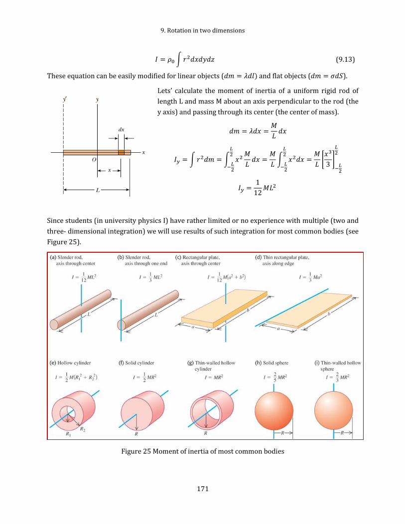
9. Rotation in two dimensions
171
𝐼 = 𝜌0 ∫ 𝑟2𝑑𝑥𝑑𝑦𝑑𝑧 (9.13)
These equation can be easily modified for linear objects (𝑑𝑚 = 𝜆𝑑𝑙) and flat objects (𝑑𝑚 = 𝜎𝑑𝑆).
Lets’ calculate the moment of inertia of a uniform rigid rod of
length L and mass M about an axis perpendicular to the rod (the
y axis) and passing through its center (the center of mass).
𝑑𝑚 = 𝜆𝑑𝑥 =𝑀
𝐿𝑑𝑥
𝐼𝑦 = ∫ 𝑟2𝑑𝑚 = ∫ 𝑥2𝑀
𝐿𝑑𝑥
𝐿2
−𝐿2
=𝑀
𝐿∫ 𝑥2𝑑𝑥
𝐿2
−𝐿2
=𝑀
𝐿[𝑥3
3]
−𝐿2
𝐿2
𝐼𝑦 =1
12𝑀𝐿2
Since students (in university physics I) have rather limited or no experience with multiple (two and
three- dimensional integration) we will use results of such integration for most common bodies (see
Figure 25).
Figure 25 Moment of inertia of most common bodies

9.7 Potential energy of a rigid body
172
Suppose we want to find the rotational inertia 𝐼 of a body of mass 𝑀 about a given axis. In principle,
we can always find 𝐼 with the integration. However, there is a shortcut if we happen to already know
the rotational inertia 𝐼𝑐𝑚 of the body about a parallel axis that extends through the body's center of
mass. Let ℎ be the perpendicular distance between the given axis and the axis through the center of
mass (remember these two axes must be parallel). Then the rotational inertia 𝐼 about the given axis
is
𝐼 = 𝐼𝑐𝑚 + 𝑚ℎ2
This equation is known as the parallel-axis theorem.
9.7 Potential energy of a rigid body
Gravitational potential energy of a rigid body can be written as an infinite sum over all mass elements
𝑚𝑖 as
𝑈 = 𝑚1𝑔𝑦1 + 𝑚2𝑔𝑦2 + 𝑚3𝑔𝑦3 + ⋯ = (𝑚1𝑦1 + 𝑚2𝑦2 + 𝑚3𝑦3 + ⋯ )𝑔
However, having the definition for the center of mass (in 𝑦 −direction)
𝑦𝑐𝑚 =𝑚1𝑦1 + 𝑚2𝑦2 + 𝑚3𝑦3 + ⋯
𝑚1 + 𝑚2 + 𝑚3 + ⋯
together with definition for the total mass 𝑀 = 𝑚1 + 𝑚2 + 𝑚3 + ⋯, one has
𝑚1𝑦1 + 𝑚2𝑦2 + 𝑚3𝑦3 + ⋯ = 𝑀𝑦𝑐𝑚
Combining this with the previous equation for 𝑈, we get
𝑈 = 𝑀𝑔𝑦𝑐𝑚 (9.14)
where 𝑦𝑐𝑚 is the vertical coordinate of the center of mass.

9. Rotation in two dimensions
173
9.8 Examples
Example 9-1
The angular velocity of helicopter blades (a rotor) changes from 320 rev/min to 225 rev/min in 5.0 s
as the rotor slows down to rest.
a) What time interval is required for the blades to come to rest from their initial angular velocity
of 320 rev/min?
b) How many revolutions do the blades make in coming to rest from the initial 320 rev/min?
SOLUTION:
1. Physics – rotation with constant angular acceleration
2. The basic equations
𝜃 = 𝜃0 + 𝜔0𝑡 +1
2𝛼𝑡2
𝜔 = 𝜔0 + 𝛼𝑡
3. Let’s note that the angular acceleration for the problem can be found from the given information
(change for angular velocity from 𝜔1 to 𝜔2 in Δ𝑡 time interval), namely
𝛼 =𝜔2 − 𝜔1
Δ𝑡
The first unknown (the time to stop) can be found from the second equation of motion (𝜔 = 𝜔0 + 𝛼𝑡)
using the condition 𝜔𝑓 = 0, and the second question can be easily answered using the first equation
of motion with constant angular acceleration
4. Let 𝑡𝑓 be the time required to stop. Then
𝑡𝑓 =𝜔𝑓 − 𝜔0
𝛼= −
𝜔0
𝛼
Then the total angular displacement during this time is
𝜃 = 𝜃0 + 𝜔0𝑡𝑓 +1
2𝛼𝑡𝑓
2
5. Calculations
We better work with SI units. Then
320𝑟𝑒𝑣
𝑚𝑖𝑛= 320
𝑟𝑒𝑣
𝑚𝑖𝑛(
2𝜋 𝑟𝑎𝑑
𝑟𝑒𝑣) (
1 𝑚𝑖𝑛
60 𝑠) = 33.5
𝑟𝑎𝑑
𝑠,
225𝑟𝑒𝑣
𝑚𝑖𝑛= 225
𝑟𝑒𝑣
𝑚𝑖𝑛(
2𝜋 𝑟𝑎𝑑
𝑟𝑒𝑣) (
1 𝑚𝑖𝑛
60 𝑠) = 23.6
𝑟𝑎𝑑
𝑠
𝛼 =(23.6 − 33.5) 𝑟𝑎𝑑 𝑠⁄
5 𝑠= −1.98 𝑟𝑎𝑑 𝑠2⁄

9.8 Examples
174
𝑡𝑓 = −33.5 𝑟𝑎𝑑 𝑠⁄
−1.98 𝑟𝑎𝑑 𝑠2⁄= 16.8 𝑠
𝜃 = 0 + 33.5𝑟𝑎𝑑
𝑠∙ 16.8 𝑠 +
1
2(−1.98 𝑟𝑎𝑑 𝑠2⁄ ) ∙ (16.8 𝑠)2 = 282 𝑟𝑎𝑑 𝑜𝑟
282 𝑟𝑎𝑑
2𝜋= 45 𝑟𝑒𝑣.
6. Looking back.
Units are correct. Both time and number of revolutions seems reasonable.
Example 9-2
What is the linear speed of a point (in mph)
a) on Earth's equator?
b) on northern pole?
c) at latitude of Norfolk? (coordinates of Norfolk are about 36°N and 76°W)
SOLUTION:
SOLUTION 1 (the easiest)
By definition speed = distance/time. Let’s consider circular motion with radius R and period (time)
T. Then distance = circumference = 2𝜋𝑅. And speed on Earth’s equator (𝑅 = 𝑅𝐸)
𝑣 =2𝜋𝑅
𝑇=
2 ∙ 3.1415 ∙ 6.37 ∙ 106𝑚
24 ℎ= 1.667 ∙ 106
𝑚
ℎ= 1.667 ∙ 106
𝑚
ℎ(
1 𝑚𝑖𝑙𝑒
1609 𝑚) = 1036 𝑚𝑝ℎ
Since rotational radius depend on the latitude as 𝑅 = 𝑅𝐸 cos 𝜃 we can easily calculate speeds for
Norfolk VA and the Northern pole.
SOLUTION 2 (connecting angular and linear variables)
1. Physics – connecting rotational and translational variables.
2. The basic equations
𝑣 = 𝜔𝑅
3. We know that the one revolution 𝜃 = 2𝜋 of the planet takes 24 hours.
Then the angular speed
𝜔 =2𝜋
𝑇
and the linear speed
𝑣 = 𝜔𝑅 =2𝜋
𝑇𝑅
4. The radius of revolution depends on latitude as 𝑅 = 𝑅𝐸 cos 𝛽 (e.g. angle 𝛽 = 360 for Norfolk). Thus
𝑣 = 2𝜋𝑅𝐸
𝑇cos 𝛽
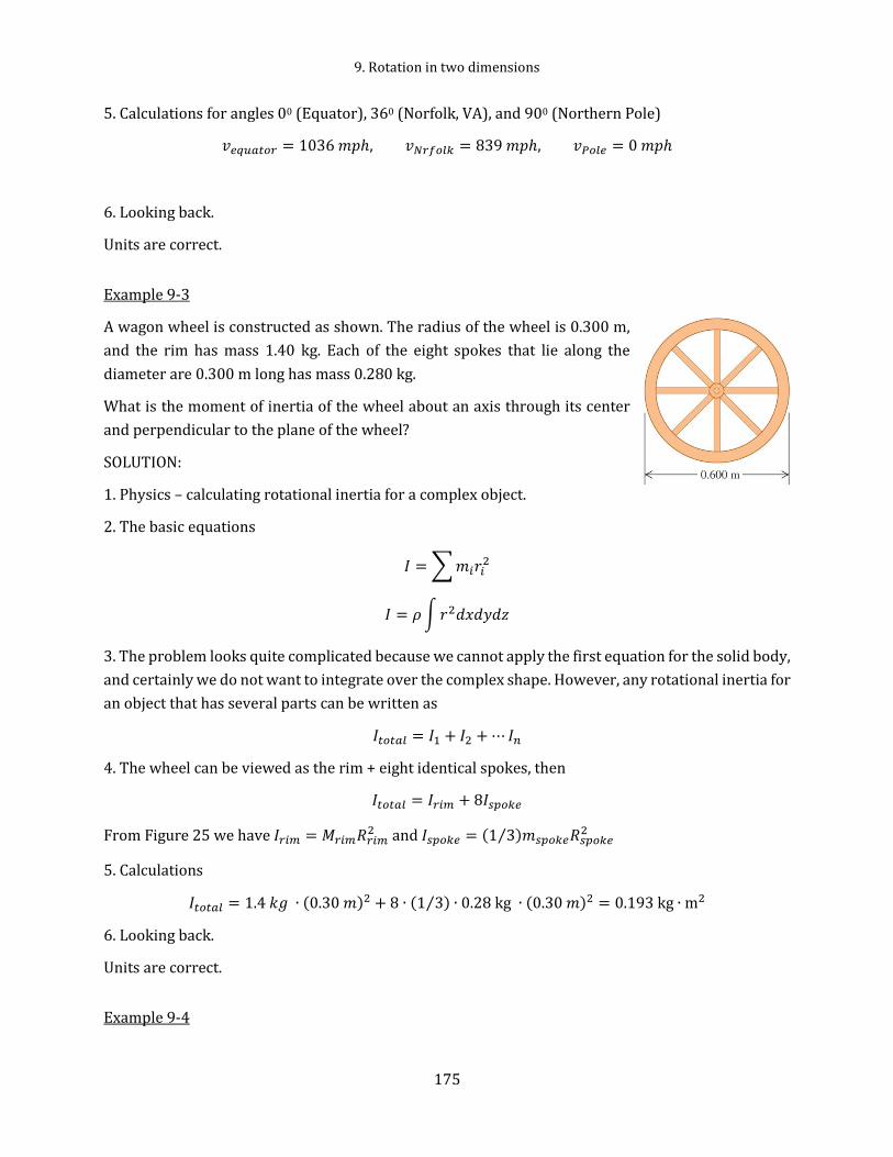
9. Rotation in two dimensions
175
5. Calculations for angles 00 (Equator), 360 (Norfolk, VA), and 900 (Northern Pole)
𝑣𝑒𝑞𝑢𝑎𝑡𝑜𝑟 = 1036 𝑚𝑝ℎ, 𝑣𝑁𝑟𝑓𝑜𝑙𝑘 = 839 𝑚𝑝ℎ, 𝑣𝑃𝑜𝑙𝑒 = 0 𝑚𝑝ℎ
6. Looking back.
Units are correct.
Example 9-3
A wagon wheel is constructed as shown. The radius of the wheel is 0.300 m,
and the rim has mass 1.40 kg. Each of the eight spokes that lie along the
diameter are 0.300 m long has mass 0.280 kg.
What is the moment of inertia of the wheel about an axis through its center
and perpendicular to the plane of the wheel?
SOLUTION:
1. Physics – calculating rotational inertia for a complex object.
2. The basic equations
𝐼 = ∑ 𝑚𝑖𝑟𝑖2
𝐼 = 𝜌 ∫ 𝑟2𝑑𝑥𝑑𝑦𝑑𝑧
3. The problem looks quite complicated because we cannot apply the first equation for the solid body,
and certainly we do not want to integrate over the complex shape. However, any rotational inertia for
an object that has several parts can be written as
𝐼𝑡𝑜𝑡𝑎𝑙 = 𝐼1 + 𝐼2 + ⋯ 𝐼𝑛
4. The wheel can be viewed as the rim + eight identical spokes, then
𝐼𝑡𝑜𝑡𝑎𝑙 = 𝐼𝑟𝑖𝑚 + 8𝐼𝑠𝑝𝑜𝑘𝑒
From Figure 25 we have 𝐼𝑟𝑖𝑚 = 𝑀𝑟𝑖𝑚𝑅𝑟𝑖𝑚2 and 𝐼𝑠𝑝𝑜𝑘𝑒 = (1 3⁄ )𝑚𝑠𝑝𝑜𝑘𝑒𝑅𝑠𝑝𝑜𝑘𝑒
2
5. Calculations
𝐼𝑡𝑜𝑡𝑎𝑙 = 1.4 𝑘𝑔 ∙ (0.30 𝑚)2 + 8 ∙ (1 3⁄ ) ∙ 0.28 kg ∙ (0.30 𝑚)2 = 0.193 kg ∙ m2
6. Looking back.
Units are correct.
Example 9-4

9.8 Examples
176
The pulley (a solid cylinder) has radius 0.160 m and mass of 1.0 kg. The rope
does not slip on the pulley rim. Use energy methods to calculate the speed
of the 4.0-kg block just before it strikes the floor.
SOLUTION:
1. Physics – conservation of energy for translational and rotational motion
in presence of gravitational force.
2. The basic equations
𝐾𝑖 + 𝑈𝑖 = 𝐾𝑓 + 𝑈𝑓
𝐾𝑡 =1
2𝑚𝑣2, 𝐾𝑟 =
1
2𝐼𝜔2, 𝑈𝑔 = 𝑚𝑔ℎ
3. There is a system with three connected parts, so we have to include every part into equation for
conservation of energy.
Let’s use notations 𝑚 for 2,0 kg block, 𝑀 for 4.0 kg block, and 𝐼 for the pulley. Then
𝐾𝑚𝑖 + 𝑈𝑔𝑚𝑖 + 𝐾𝑀𝑖 + 𝑈𝑔𝑀𝑖 + 𝐾𝐼𝑖 + 𝑈𝑔𝐼𝑖 = 𝐾𝑚𝑓 + 𝑈𝑔𝑚𝑓 + 𝐾𝑀𝑓 + 𝑈𝑔𝑀𝑓 + 𝐾𝐼𝑓 + 𝑈𝑔𝐼𝑓
4. Initially the system is at rest, so all initial kinetic energies are zero. We are going to count the
gravitational potential energy from the ground. Let’s also note that gravitational potential energy of
the pulley does not change. With this in mind we have
𝑈𝑔𝑀𝑖 = 𝐾𝑚𝑓 + 𝑈𝑔𝑚𝑓 + 𝐾𝑀𝑓 + 𝐾𝐼𝑓
or being more specific
𝑀𝑔ℎ =1
2𝑚𝑣2 +
1
2𝑀𝑣2 +
1
2𝐼𝜔2 + 𝑚𝑔ℎ
where h=5.0 m.
Since the rope does not slip, then 𝑣 = 𝜔𝑅. For a solid cylinder 𝐼 = 0.5𝑀𝑐𝑅2. Then we can rewrite the
last equation as
(𝑀 − 𝑚)𝑔ℎ =1
2𝑚𝑣2 +
1
2𝑀𝑣2 +
1
2(
1
2𝑀𝑐𝑅2)
𝑣2
𝑅2=
1
2𝑣2 (𝑚 + 𝑀 +
1
2𝑀𝑐)
Solving for 𝑣 gives
𝑣 = √2(𝑀 − 𝑚)𝑔ℎ
𝑚 + 𝑀 +12 𝑀𝑐
5. Calculations

9. Rotation in two dimensions
177
𝑣 = √2(4.0 𝑘𝑔 − 2.0 𝑘𝑔)9.8 𝑚 𝑠2⁄ ∙ 5 𝑚
(2.0 + 4.0 + 0.5 ∙ 1.0) 𝑘𝑔= 5.5 𝑚/𝑠
6. The units are correct. For 𝑀𝑐 = 0 we get the answer for example 7-7.

10.1 Torque
178
10 Dynamics of rotational motion
10.1 Torque
Let us now move on to consider the dynamics of rotation. Here a new concept, force, must be
introduced. Let us inquire whether we can invent something which we shall call the torque (Latin
torquere, to twist) which bears the same relationship to rotation as force does to linear movement. A
force is the thing that is needed to make linear motion, and the thing that makes something rotate is
a "rotary force" or a "twisting force," i.e., a torque. Qualitatively, a torque is a "twist". What is a torque
quantitatively?
Here is some intuitive approach to define torque. A doorknob is located as far as possible from the
door's hinge line for a good reason. If you want to open a heavy door, you must certainly apply a force:
that alone, however, is not enough. Where you apply that force and in what direction you push are also
important.
Figure shows a cross section of a body that is free to rotate about an
axis passing through O and perpendicular to the cross section. A force
�⃗� is applied at point P, whose position relative to O is defined by a
position vector 𝑟. The directions of vectors �⃗� and 𝑟 make an angle 𝜙
with each other. (For simplicity, we consider only forces that have no
component parallel to the rotation axis: thus �⃗� is in the plane of the
page.).
To determine how �⃗� results in a rotation of the body around the
rotation axis, we resolve �⃗� into two components. One component,

10. Dynamics of rotational motion
179
called the parallel (radial) component 𝐹∥ points along 𝑟 . This component does not cause rotation
because it acts along a line that extends through O. (If you pull on a door parallel to the plane of the
door, you do not rotate the door.) The other component of �⃗�, called the perpendicular (tangential)
component 𝐹⊥, is perpendicular to 𝑟 and has magnitude 𝐹⊥ = 𝐹 sin 𝜙. This component does cause
rotation. (If you pull on a door perpendicular to its plane, you can rotate the door.)
The ability of �⃗� to rotate the body depends not only on the magnitude of its tangential component 𝐹⊥
, but also on just how far from O the force is applied. To include both these factors, we define a quantity
called torque 𝜏 as the product of the two factors and write it as
𝜏 = 𝑟𝐹 sin 𝜙 = 𝑟𝐹⊥
Torque, which comes from the Latin word meaning "to twist," may be loosely identified as the turning
or twisting action of the force �⃗�. When you apply a force to an object such as a screwdriver or torque
wrench with the purpose of turning that object, you are applying a torque.
The SI unit of torque is the newton-meter (Nm). Caution: The newton-meter is also the unit of work.
Torque and work however, are quite different quantities and must not be confused. Work is often
expressed in joules (1 J = 1 Nm), but torque never is.
Now we can write a general definition for torque based on a vector product of two vectors, namely
𝜏 = 𝑟 × �⃗� (10.1)
This definition has both magnitude and direction because torque is a vector.
At this point we need to talk more about vector product of two vectors
10.2 Vector Product
The vector product of two vectors 𝐴 and �⃗⃗�, also called a cross product, is denoted by 𝐴 × �⃗⃗�. The vector
product is itself a vector.
𝐶 = 𝐴 × �⃗⃗� (10.2)
The magnitude of the vector (cross) product is defined as
𝐶 = 𝐴𝐵 sin 𝜙 (10.3)
We measure the angle 𝜙 from 𝐴 toward �⃗⃗�, and take it to be the smallest of two possible angles, so 𝜙
ranges from 00 to 1800 (the magnitude of 𝐶 is always positive)
Some properties of the cross product
𝐴 × 𝐴 = 0
𝐴 × �⃗⃗� = −�⃗⃗� × 𝐴
𝐴 × (�⃗⃗� + 𝐶) = 𝐴 × �⃗⃗� + 𝐴 × 𝐶

10.3 Torque as a vector product
180
𝑑
𝑑𝑡(𝐴 × �⃗⃗�) =
𝑑𝐴
𝑑𝑡× �⃗⃗� + 𝐴 ×
𝑑�⃗⃗�
𝑑𝑡.
There are always two directions perpendicular to a given plane, one on each side of a plane. The
direction of the vector product follows the right-hand rule.
Imagine rotating vector 𝐴 about the perpendicular line until it is align with
�⃗⃗�, choosing the smaller of the two possible angles between 𝐴 and �⃗⃗�. Curl the
fingers of your right hand around the perpendicular line so that the
fingertips point in the direction of rotation; your thumb will then point in
the direction of 𝐴 × �⃗⃗�. Figure shows this right-hand rule
If we know the components of 𝐴 and �⃗⃗�, we can calculate the components of the vector product 𝐶 =
𝐴 × �⃗⃗� using properties of unit vectors
𝑖̂ × 𝑖̂ = 𝑗̂ × 𝑗̂ = �̂� × �̂� = 0
𝑖̂ × 𝑗̂ = −𝑗̂ × 𝑖̂ = �̂�
𝑗̂ × �̂� = −�̂� × 𝑗̂ = 𝑖 ̂
�̂� × 𝑖̂ = −𝑖̂ × �̂� = 𝑗 ̂
we get
𝐶 = 𝐴 × �⃗⃗� = (𝐴𝑥𝑖̂ + 𝐴𝑦𝑗̂ + 𝐴𝑧�̂�) × (𝐵𝑥𝑖̂ + 𝐵𝑦𝑗̂ + 𝐵𝑧�̂�)
= (𝐴𝑦𝐵𝑧 − 𝐴𝑧𝐵𝑦)𝑖̂ + (𝐴𝑧𝐵𝑥 − 𝐴𝑥𝐵𝑧)𝑗̂ + (𝐴𝑥𝐵𝑦 − 𝐴𝑦𝐵𝑥)�̂�
Thus, the components of the resulting vector are given by
𝐶𝑥 = 𝐴𝑦𝐵𝑧 − 𝐴𝑧𝐵𝑦
𝐶𝑦 = 𝐴𝑧𝐵𝑥 − 𝐴𝑥𝐵𝑧
𝐶𝑧 = 𝐴𝑥𝐵𝑦 − 𝐴𝑦𝐵𝑥 (10.4)
10.3 Torque as a vector product
The torque 𝜏 acting on acting on the particle relative to the fixed point 0 is a vector quantity
𝜏 = 𝑟 × �⃗�
We can evaluate the vector (or cross) product in this definition of by using
𝜏 = 𝑟𝐹 sin 𝜙 = 𝑟𝐹⊥ (10.5)
or in the component form (keeping in mind that normally we place 𝑟 and �⃗� in the xy-plane),
𝜏𝑧 = 𝑟𝑥𝐹𝑦 − 𝑟𝑦𝐹𝑥 (10.6)
10.4 Newton’s Second Law for rotation
A torque can cause rotation of a rigid body, as when you use a torque to rotate a door.

10. Dynamics of rotational motion
181
Let’s consider the simple situation shown in figure to the left.
The rigid body there consists of a particle of mass m on one end
of a massless rod of length r. The rod can move only by rotating
about its other end, around a rotation axis (an axle) that is
perpendicular to the plane of the page. Thus, the particle can
move only in a circular path that has the rotation axis at its
center.
A force �⃗� acts on the particle. However, because the particle can
move only along the circular path, only the tangential
component 𝐹𝑡 of the force (the component that is tangent to the
circular path) can accelerate the particle along the path. We can
relate 𝐹𝑡 to the particle's tangential acceleration at along the
path with Newton's second law, writing
𝐹𝑡 = 𝑚𝑎𝑡
The torque acting on the particle is
𝜏 = 𝐹𝑡𝑟 = 𝑚𝑎𝑡𝑟
From 𝑎𝑡 = 𝛼𝑟 we can write this as
𝜏 = 𝑚(𝛼𝑟)𝑟 = (𝑚𝑟2)𝛼
The quantity in parentheses on the right side of equation above is the rotational inertia of the particle
(𝐼 = 𝑚𝑟2) about the rotation axis. Thus,
𝜏 = 𝐼𝛼
We can easily extend this equation to any rigid body rotating about a fixed axis, because any such
body can always be analyzed as an assembly of single particles.
𝜏1𝑧 + 𝜏2𝑧 + ⋯ = 𝐼1𝛼𝑧 + 𝐼2𝛼𝑧 + ⋯ = (𝐼1 + 𝐼2 + ⋯ )𝛼𝑧 = 𝐼𝛼𝑧
Thus we can write rotational analog of Newton’s second law for a rigid body (We assume that the
angular acceleration 𝛼 is the same for all particles in the body). For rotations in xy-plane
∑ 𝜏𝑧 = 𝜏𝑛𝑒𝑡,𝑧 = 𝐼𝛼𝑧 (10.7)
Generally in vector form for rotation in three dimensional space
𝜏 = 𝐼�⃗� (10.8)
Just as Newton's second law says that the net force on a particle equals the particle's mass times its
acceleration, equation above says that the net torque on a rigid body equals the body's moment of
inertia about the rotation axis times its angular acceleration. Thus, this equation is the rotational
analog of Newton’s second law for linear motion �⃗� = 𝑚�⃗�.

10.5 Rolling
182
This equation doesn't apply to a rotating tank of water or a swirling tornado of air, different parts of
which have different angular accelerations.
The torque on each particle is due to the net force on that particle, which is the vector sum of external
and internal forces. According to Newton's third law, the internal forces that any pair of particles in
the rigid body exerts on each other are equal and opposite. If these forces act along the line joining
the two particles, their lever arms with respect to any axis are also equal. So the torques for each such
pair are equal and opposite and add to zero. Hence all the internal torques add to zero, so the sum in
𝜏𝑛𝑒𝑡,𝑧 includes only the torques of the external forces.
10.5 Rolling
We can extend our analysis of the rotational motion to some cases in which the axis of rotation moves.
When that happens, the motion of the body is combined translation and rotation. The key to
understanding such situations is this: Every possible motion of a rigid body can be represented as a
combination of translational motion of the center of mass and rotation about an axis through the
center of mass. This is true even when the center of mass accelerates, so that it is not at rest in any
inertial frame.
Consider a system with two particles (extension to 𝑛 particles is evident). The kinetic energy 𝐾 of a
system of particles is the sum of the kinetic energies of the individual particles:
𝐾 = 𝐾1 + 𝐾2 =1
2𝑚1𝑣1
2 +1
2𝑚2𝑣2
2
The position of a particle can be written as the sum of two vectors, the position of the center of mass
and the position of the particle relative to the center of mass
𝑟 = 𝑟𝑐𝑚 + 𝑠
Then differentiating this vector we get the velocity of a particle as
�⃗� = �⃗�𝑐𝑚 + �⃗⃗�
where �⃗�𝑐𝑚 is the velocity of the center of mass and �⃗⃗� is the velocity of the particle relative to the center
of mass. Substituting it into equation for the kinetic energy, we obtain
𝐾 =1
2𝑚1(�⃗�𝑐𝑚 + �⃗⃗�1)2 +
1
2𝑚2(�⃗�𝑐𝑚 + �⃗⃗�2)2
=1
2𝑚1𝑣𝑐𝑚
2 +1
2𝑚2𝑣𝑐𝑚
2 +1
2𝑚1𝑢1
2 +1
2𝑚2𝑢2
2 + 𝑚1�⃗�𝑐𝑚�⃗⃗�1 + 𝑚2�⃗�𝑐𝑚�⃗⃗�2
=1
2(𝑚1 + 𝑚2)𝑣𝑐𝑚
2 +1
2𝑚1𝑢1
2 +1
2𝑚2𝑢2
2 + �⃗�𝑐𝑚(𝑚1�⃗⃗�1 + 𝑚2�⃗⃗�2)
The quantity 𝑚1�⃗⃗�1 + 𝑚2�⃗⃗�2 is equal to
𝑚1�⃗⃗�1 + 𝑚2�⃗⃗�2 =𝑑
𝑑𝑡(𝑚1𝑠1 + 𝑚2𝑠2) =
𝑑
𝑑𝑡((𝑚1 + 𝑚2)𝑠𝑐𝑚)

10. Dynamics of rotational motion
183
where 𝑠𝑐𝑚 is the position of the center of mass relative to the center of mass, and clearly 𝑠𝑐𝑚 = 0.
Then 𝑚1�⃗⃗�1 + 𝑚2�⃗⃗�2 = (𝑚1 + 𝑚2)�⃗⃗�𝑐𝑚 = 0 (the velocity of anything relative to itself is always equal to
zero.) It follows that
𝐾 =1
2(𝑚1 + 𝑚2)𝑣𝑐𝑚
2 +1
2(𝑚1𝑢1
2 + 𝑚2𝑢22)
The last term is the sum of the kinetic energies calculated by using their speeds with respect to the
center of mass; this is just the kinetic energy of rotation with the same angular speed 𝜔 = 𝑢 𝑟⁄ , then
1
2(𝑚1𝑢1
2 + 𝑚2𝑢22) =
1
2(𝑚1𝜔2𝑟1
2 + 𝑚2𝜔2𝑟22) =
1
2(𝑚1𝑟1
2 + 𝑚2𝑟22)𝜔2 =
1
2(𝐼1 + 𝐼2)𝜔2
Thus, the kinetic energy is the sum of a part associated with motion of the center of mass and a part
associated with rotation about an axis through the center of mass:
𝐾 =1
2(𝑚1 + 𝑚2)𝑣𝑐𝑚
2 +1
2(𝐼1 + 𝐼2)𝜔2
For rigid bodies the rotational inertia does not change during motion. Thus, for any system of particles
or a rigid body we can write
𝐾 =1
2𝑀𝑣𝑐𝑚
2 +1
2𝐼𝑐𝑚𝜔2 (10.9)
where 𝑀 is the total mass of the system, and 𝐼𝑐𝑚 is the rotational inertia associated with rotation
about an axis through the center of mass.
10.5.1 Smooth rolling
An important case of combined translation and rotation is rolling without slipping, such as the motion
of a wheel. The wheel is symmetrical, so its center of mass is at its geometric center. We view the
motion in an inertial frame of reference in which the surface on which the wheel rolls is at rest. In this
frame, the point on the wheel that contacts the surface must be instantaneously at rest so that it does
not slip. Hence the velocity �⃗�1′ of the point of contact relative to the center of mass must have the same
magnitude but opposite direction as the center-of-mass velocity �⃗�𝑐𝑚′. If the radius of the wheel is 𝑅
and its angular speed about the center of mass is 𝜔, then the magnitude of �⃗�𝑐𝑚′ is 𝑅𝜔; hence we must
have 𝑣𝑐𝑚 = 𝑅𝜔 for smooth (without slipping) rolling motion.

10.5 Rolling
184
As the figure above shows, the velocity of a point on the wheel is the vector sum of the velocity of the
center of mass and the velocity of the point relative to the center of mass. Thus, while point 1, the
point of contact, is instantaneously at rest, point 3 at the top of the wheel is moving forward twice as
fast as the center of mass, and points 2 and 4 at the sides have velocities at 450 to the horizontal.
Now, in the kinetic energy of rolling
𝐾 =1
2𝑀𝑣𝑐𝑚
2 +1
2𝐼𝑐𝑚𝜔2
we have
𝑣𝑐𝑚 = 𝜔𝑅 (10.10)
or the linear and angular velocities are not independent.
10.5.2 The forces of rolling
If a wheel rolls at constant speed it has no tendency to slide at the point of contact P, and thus no
frictional force acts there. However, if a net force acts on the rolling wheel to speed it up or to slow it
down, then that net force causes acceleration 𝑎𝑐𝑚 of the center of mass along the direction of travel.
It also causes the wheel to rotate faster or slower, which means it causes an angular acceleration 𝛼
about the center of mass. These accelerations tend to make the wheel slide at P. Thus, a frictional force
must act on the wheel at P to oppose that tendency.
If the wheel does not slide, the force is a static frictional force 𝑓𝑠 and the motion is smooth rolling. We
can then relate the magnitudes of the linear acceleration and the angular acceleration by
differentiating 𝑣𝑐𝑚 = 𝜔𝑅 with respect to time (with 𝑅 held constant). So, for smooth rolling we have
𝑎𝑐𝑚 = 𝛼𝑅
Let’s study rolling down a ramp.
This figure shows a round uniform body of mass 𝑀 and radius 𝑅 rolling
smoothly down a ramp at angle , along an x axis. We want to find
expressions for the body's acceleration 𝑎𝑐𝑚 down the ramp. We do this
by using Newton's second law in both its linear version (𝐹𝑛𝑒𝑡 = 𝑀𝑎)
and its angular version (𝜏𝑛𝑒𝑡 = 𝐼𝛼).
We start by drawing the forces on the body
1. The gravitational force �⃗�𝑔 on the body is directed downward. The
tail of the vector is placed at the center of mass of the body. The
component along the ramp is 𝑓𝑔 sin 𝜃, which is equal to 𝑀𝑔 sin 𝜃.
2. A normal force �⃗⃗⃗� is perpendicular to the ramp. It acts at the point of contact P, but the vector has
been shifted along its direction until its tail is at the body's center of mass.

10. Dynamics of rotational motion
185
3. A static frictional force 𝑓𝑠 acts at the point of contact P and is directed up the ramp. (Do you see
why? If the body were to slide at P, it would slide down the ramp. Thus, the frictional force opposing
the sliding must be up the ramp.) We can write Newton's second law for components along the x axis
in
𝑓𝑠 − 𝑀𝑔 sin 𝜃 = 𝑀𝑎𝑐𝑚.
This equation contains two unknowns, 𝑓𝑠 and 𝑎𝑐𝑚. We should not assume that 𝑓𝑠 is at its maximum
value 𝑓𝑠,𝑚𝑎𝑥. All we know is that the value of 𝑓𝑠, is just right for the body to roll smoothly down the
ramp, without sliding.
We now wish to apply Newton's second law in angular form to the body's rotation about its center of
mass 𝜏𝑛𝑒𝑡 = 𝐼𝛼. The frictional force produces a torque 𝑅𝑓𝑠, which is positive because it tends to rotate
the body counterclockwise in Figure. Forces�⃗�𝑔 and �⃗⃗⃗� produce zero torques (do you see why?). So we
can write the angular form of Newton's second law about an axis through the body's center of mass
as
𝑅𝑓𝑠 = 𝐼𝑐𝑚𝛼.
This equation contains two unknowns, 𝑓𝑠 and 𝛼.
Because the body is rolling smoothly, we can use 𝑎𝑐𝑚 = 𝛼𝑅 to relate the unknown accelerations. But
we must be cautious because here 𝑎𝑐𝑚 is negative (in the negative direction of the x axis) and 𝛼 is
positive (counterclockwise). Thus we substitute −𝑎𝑐𝑚/𝑅 for 𝛼, and
𝑓𝑠 = −𝐼𝑐𝑚
𝑎𝑐𝑚
𝑅2
Substituting it to the first equation 𝑓𝑠 − 𝑀𝑔 sin 𝜃 = 𝑀𝑎𝑐𝑚 we find
𝑎𝑐𝑚 = −𝑔 sin 𝜃
1 + 𝐼𝑐𝑚 𝑀𝑅2⁄
We can use this equation to find the linear acceleration of any body rolling smoothly (without
slipping) along an incline.
For most rolling objects the rotational inertia 𝐼 can be written as 𝐼 = 𝛽𝑀𝑅2 where 𝛽 is a coefficient
specific for specific shape (for example 𝛽 = 2 5⁄ for a solid sphere). Then
𝑎𝑐𝑚 = −𝑔 sin 𝜃
1 + 𝛽
and
𝑓𝑠 =𝛽
1 + 𝛽𝑀𝑔 sin 𝜃
Let’s find the static frictional force needed to prevent slipping
𝜇𝑠𝑀𝑔 cos 𝜃 ≥𝛽
1 + 𝛽𝑀𝑔 sin 𝜃

10.6 Translation and rotation dynamics
186
or
𝜇𝑠 ≥𝛽
1 + 𝛽tan 𝜃.
10.6 Translation and rotation dynamics
Rolling is a nice example of combined translation and rotation dynamics. Earlier we demonstrated
(section 8.3) that for a body with total mass 𝑀, the acceleration of the center of mass is the same as
that of a point mass 𝑀 acted on by all the external forces on the actual body:
∑ �⃗�𝑒𝑥𝑡 = 𝑀�⃗�𝐶𝑀
The rotational motion about the center of mass is described by the rotational analog of Newton’s
second law, Eq. (10.7)
∑ 𝜏𝑧 = 𝐼𝑐𝑚�⃗�𝑧
provided the following two conditions are met for combined translation and rotation motion
1. The axis through the center of mass must be an axis of symmetry.
2. The axis must not change direction.
These conditions are satisfied for many types of rotation. We can now solve dynamics problems
involving a rigid body that undergoes translational and rotational motions at the same time, if the
rotation axis satisfies the two conditions just mentioned
10.7 Work and Power in Rotational Motion
In chapter 6 we related change in kinetic energy of a moving particle with force acting on that particle
along some path
∆𝐾 = 𝐾𝑓 − 𝐾𝑖 = ∫ �⃗� ∙ 𝑑𝑟𝑓
𝑖
= 𝑊(𝑖 → 𝑓)
Then the power was defined as
𝑃 =𝑑𝑊
𝑑𝑡= �⃗� ∙ �⃗�
We can easily derive similar equations for a rotational situation. Here are just resulting equations
∆𝐾 = 𝐾𝑓 − 𝐾𝑖 =1
2𝐼𝜔𝑓
2 −1
2𝐼𝜔𝑖
2 = ∫ 𝜏𝑧𝑑𝜃𝑓
𝑖
= 𝑊(𝑖 → 𝑓)
When 𝜏𝑧 is constant
∆𝐾 = 𝜏𝑧(𝜃𝑓 − 𝜃𝑖) = 𝑊(𝑖 → 𝑓)
The rotational equivalent of power for rotational motion is

10. Dynamics of rotational motion
187
𝑃 =𝑑𝑊
𝑑𝑡= 𝜏𝑧𝜔𝑧
10.8 Angular momentum
Although we have only considered the special case of a rigid body thus far, the properties of torques
and their mathematical relationships are interesting also even when an object is not rigid. In fact, we
can prove a very remarkable theorem: just as external force is the rate of change of a quantity 𝑝, which
we call the total momentum of a collection of particles, the external torque is the rate of change of a
quantity �⃗⃗� which we call the angular momentum of the group of particles.
To prove this, we shall suppose that there is a system of particles on which there are some forces
acting and find out what happens to the system as a result of the torques due to these forces. First, of
course, we should consider just one particle of mass 𝑚 moving around an axis 𝑂; the particle is not
necessarily rotating in a circle about 𝑂, it may be moving in an ellipse, like a planet going around the
sun, or in some other curve. The torque is
𝜏𝑧 = 𝑥𝐹𝑦 − 𝑦𝐹𝑥
and using Newton’s second law we can write it as
𝜏𝑧 = 𝑥𝑚𝑑2𝑦
𝑑𝑡2− 𝑦𝑚
𝑑2𝑥
𝑑𝑡2
Now, although this does not appear to be the derivative of any simple quantity, it is in fact the
derivative of the quantity
𝑥𝑚 (𝑑𝑦
𝑑𝑡) − 𝑦𝑚 (
𝑑𝑥
𝑑𝑡)
𝑑
𝑑𝑡[𝑥𝑚 (
𝑑𝑦
𝑑𝑡) − 𝑦𝑚 (
𝑑𝑥
𝑑𝑡)] = 𝑥𝑚 (
𝑑2𝑦
𝑑𝑡2 ) + (𝑑𝑥
𝑑𝑡) 𝑚 (
𝑑𝑦
𝑑𝑡) − 𝑦𝑚 (
𝑑2𝑥
𝑑𝑡2 ) − (𝑑𝑦
𝑑𝑡) 𝑚 (
𝑑𝑥
𝑑𝑡)
= 𝑥𝑚𝑑2𝑦
𝑑𝑡2− 𝑦𝑚
𝑑2𝑥
𝑑𝑡2
So it is true that the torque is the rate of change of something with time! So we pay attention to the
"something," we give it a name: we call it 𝐿, the angular momentum, where for 𝑧 −component
𝐿𝑧 = 𝑥𝑚 (𝑑𝑦
𝑑𝑡) − 𝑦𝑚 (
𝑑𝑥
𝑑𝑡) = 𝑥𝑝𝑦 − 𝑦𝑝𝑥
So we have found that there is also a rotational analog for the momentum, and that this analog, the
angular momentum, is given by an expression in terms of the components of linear momentum that
is just like the formula for torque in terms of the force components!
Generally, in vector notation the angular momentum for a particle with constant mass m, velocity �⃗�
momentum 𝑝 and position vector 𝑟 relative to the origin 𝑂 of an inertial frame is defined as

10.8 Angular momentum
188
�⃗⃗� = 𝑟 × 𝑝 = 𝑟 × 𝑚�⃗� (10.11)
Like torque, angular momentum depends upon the position of the axis about which it is to be
calculated.
10.8.1 Conservation of angular momentum
Now we shall go on to consider what happens when there is a large number of particles, when an
object is made of many pieces with many forces acting between them and on them from the outside.
Now suppose we add the torques 𝜏𝑖 for all the particles and call it the total torque 𝜏. Now it might
seem that the total torque is a complicated thing. There are all those internal forces and all the outside
forces to be considered. But, if we take Newton's law of action and reaction to say, not simply that the
action and reaction are equal, but also that they are directed exactly oppositely along the same line,
then the two torques on the reacting objects, due to their mutual interaction, will be equal and
opposite because the lever arms for any axis are equal.
Let’s consider the total angular momentum
�⃗⃗� = �⃗⃗�1 + �⃗⃗�2 = 𝑟1 × 𝑝1 + 𝑟2 × 𝑝2
Differentiating with respect to 𝑡
𝑑
𝑑𝑡�⃗⃗� =
𝑑
𝑑𝑡(𝑟1 × 𝑝1) +
𝑑
𝑑𝑡(𝑟2 × 𝑝2)
Because
𝑑
𝑑𝑡(𝑟 × 𝑝) = �⃗� × 𝑝 + 𝑟 ×
𝑑𝑝
𝑑𝑡= 𝑟 × �⃗�
then
𝑑
𝑑𝑡�⃗⃗� =
𝑑
𝑑𝑡(𝑟1 × 𝑝1) +
𝑑
𝑑𝑡(𝑟2 × 𝑝2) = 𝑟1 × �⃗�1 + 𝑟2 × �⃗�2
Now let’s separate the effect of the internal and external forces.
�⃗�1 = �⃗�𝑛𝑒𝑡,1 = �⃗�21 + �⃗�1𝑒𝑥𝑡 , �⃗�2 = �⃗�𝑛𝑒𝑡,2 = �⃗�12 + �⃗�2
𝑒𝑥𝑡
Substituting it into equation before, we find that
𝑑
𝑑𝑡�⃗⃗� = 𝑟1 × �⃗�21 + 𝑟1 × �⃗�1
𝑒𝑥𝑡 + 𝑟2 × �⃗�12 + 𝑟2 × �⃗�2𝑒𝑥𝑡
Let’s concentrate on the internal forces where �⃗�21 = −�⃗�12 (action-reaction).

10. Dynamics of rotational motion
189
𝑟1 × �⃗�21 + 𝑟2 × �⃗�12 = 𝑟1 × �⃗�21 − 𝑟2 × �⃗�21 = (𝑟1 − 𝑟2) × �⃗�21
According to the vector diagram, vectors 𝑟1 − 𝑟2 and �⃗�21 are collinear
and their cross product is zero.
Therefore, the internal torques balance out pair by pair, and we have
the remarkable theorem that the rate of change of the total angular
momentum about any axis is equal to the external torque about that
axis!
𝜏 = ∑ 𝜏𝑖 = 𝜏𝑒𝑥𝑡 =𝑑�⃗⃗�
𝑑𝑡 (10.12)
Thus we have a very powerful theorem concerning the motion of large collections of particles, which
permits us to study the over-all motion without having to look at the detailed machinery inside. This
theorem is true for any collection of objects, whether they form a rigid body or not.
One extremely important case of the above theorem is the law of conservation of angular momentum:
if no external torques acts upon a system of particles, the angular momentum remains constant.
A special case of great importance is that of a rigid body, that is, an object of a definite shape that is just
turning around. Consider an object that is fixed in its geometrical dimensions, and which is rotating
about a fixed axis. For an object going around in a circle, the angular momentum is
𝐿𝑖 = 𝑚𝑖𝑣𝑖𝑟𝑖 = 𝑚𝑖𝑟𝑖2𝜔
or, summing over all the particles 𝑖, we get
�⃗⃗� = 𝐼�⃗⃗⃗� (10.13)
where 𝑖 is the moment of inertia. This is the analog of the law that the momentum is mass times
velocity. There is one important difference between mass and moment of inertia which is very
dramatic. The mass of an object never changes, but its moment of inertia can be changed. If we stand
on a frictionless, rotatable stand with our arms outstretched, and hold some weights in our hands as
we rotate slowly, we may change our moment of inertia by drawing our arms in, but our mass does
not change. If the external torque is zero, then the angular momentum remains constant.
𝐼1ω⃗⃗⃗1 = 𝐼2�⃗⃗⃗�2 (10.14)
Quite often in this course we consider rotational motion on 𝑥𝑦 plane, and then we can write
𝐼1𝜔1𝑧 = 𝐼2𝜔2𝑧 (10.15)
That is, if we reduce the moment of inertia, we have to increase the angular velocity.

10.9 Examples
190
10.9 Examples
Example 10-1
While exploring the castle, Exena the Exterminator is spotted by a dragon that chases her down a
hallway. Exena runs into a safe room and attempts to swing a heavy door shut before the dragon gets
her. The door is initially perpendicular to the wall, so it must be turned through 900 to be closed. The
door is 3.00 m tall and 1.25 m wide, and its mass is 200.0 kg. If Exena applies a force of 220 N at the
edge of the door and perpendicular to it, how much time does it take her to shut the door? Ignore the
friction in the hinges.
SOLUTION:
1. Physics – Newton’s second law for rotational + motion with constant angular acceleration (because
the force is constant)
2. The basic equations
𝜏 = 𝐼𝛼
𝜃 = 𝜃0 + 𝜔0𝑡 +1
2𝛼𝑡2
3. For the door 𝐼 = (1 3⁄ )𝑀𝑤2, where 𝑤 is the width of the door. Then
𝐹𝐸𝑤 =1
3𝑀𝑤2𝛼
𝜃 =𝜋
2=
1
2𝛼𝑡2
4. From the first equation
𝛼 =3𝐹𝐸
𝑀𝑤, 𝑡 = √
2𝜃
𝛼
5. Calculations
𝛼 =3 ∙ 220 𝑁
200.0 𝑘𝑔 ∙ 1.25 𝑚= 2.64
𝑁
𝑘𝑔 ∙ 𝑚= 2.64
𝑘𝑔 ∙ 𝑚 ∙ 𝑠−2
𝑘𝑔 ∙ 𝑚= 2.64
𝑟𝑎𝑑
𝑠2
𝑡 = √2 ∙ 𝜋/2
2.64 𝑟𝑎𝑑 𝑠2⁄= 1.09 𝑠
6. Units are correct both for the angular acceleration and time. It is difficult to apply common sense
to fairy tales, but with the force of 220 N (or about 50 lb) applied to the massive door (about 440 lb)
the time seems realistic.

10. Dynamics of rotational motion
191
Example 10-2
Figure shows a uniform disk, with mass 𝑀 and radius 𝑅,
mounted on a fixed horizontal axel. A block with mass 𝑚 hangs
from a massless cord that is wrapped around the rim of the
disk. Find the acceleration of the falling disk, and the tension in
the cord. The cord does not slip, and there is no friction in the
axel.
SOLUTION:
1. Physics – Newton’s second law for translational (the block)
and rotational (the disk) motions.
2. The basic equations
𝐹 = 𝑚𝑎
𝜏 = 𝐼𝛼
3. As always we must have a free-body diagram for every object in the picture. Besides we use for the
disk 𝐼 = (1 2⁄ )𝑀𝑅2, and since the cord does not slip 𝑎 = 𝛼𝑅.
4. For the falling block
𝑇 − 𝑚𝑔 = −𝑚𝑎
For the disk
−𝑅𝑇 = −𝐼𝛼 = −1
2𝑀𝑅2
𝑎
𝑅= −
1
2𝑀𝑅𝑎
These two equations have two unknowns, namely 𝑇 and 𝑎. From the second equation
𝑇 =1
2𝑀𝑎
Using it in the first equation
1
2𝑀𝑎 − 𝑚𝑔 = −𝑚𝑎 𝑎 (𝑚 +
1
2𝑀) = 𝑚𝑔
𝑎 =2𝑚
2𝑚 + 𝑀𝑔
𝑇 =𝑚𝑀
2𝑚 + 𝑀𝑔
5. Calculations
There were no data to calculate
6. Let’s analyze the answer using our past knowledge.

10.9 Examples
192
It’s clear that for massless disk the acceleration of the block must be . For 𝑀 = 0 we get
𝑎 =2𝑚
2𝑚 + 𝑀𝑔 =
2𝑚
2𝑚𝑔 = 𝑔
For a very heavy disk 𝑀 ≫ 𝑚 we get 𝑎 ≈ 0 and 𝑇 ≈ 𝑚𝑔 (also this is what we expected).
Example 10-3
A golf ball (mass of 45.93 g and diameter of 42.67 mm) starts from rest and rolls without slipping a
distance of 12.0 m down a hill towards a pond. The hill is inclined at 50.
a) What fraction of the total kinetic energy of the golf ball is due to rotation as it gets to the pond?
b) What is the speed of the golf ball at the bottom of the hill?
SOLUTION:
1. Physics – rolling, conservation of energy
2. The basic equations
𝐾𝑖 + 𝑈𝑖 = 𝐾𝑓 + 𝑈𝑓
𝐾𝑡 =1
2𝑚𝑣2, 𝐾𝑟 =
1
2𝐼𝜔2, 𝑈𝑔 = 𝑚𝑔ℎ
3. For the first question we need to find
𝐾𝑟
𝐾𝑡 + 𝐾𝑟
and the second question can be solved using conservation of energy 𝑈𝑖 = 𝐾𝑡 + 𝐾𝑟
4. Additional information: a golf ball can be treated as a solid sphere, then 𝐼 = (2 5⁄ )𝑚𝑅2 and for
rolling without slipping 𝑣 = 𝜔𝑅
𝐾𝑟 =1
2(
2
5𝑚𝑅2)
𝑣2
𝑅2=
1
5𝑚𝑣2
𝐾𝑟
𝐾𝑡 + 𝐾𝑟=
15
𝑚𝑣2
12 𝑚𝑣2 +
15
𝑚𝑣2=
2
7
Note that the answer does not depend on the hill’s incline or even shape and size.
Applying conservation of energy
𝑚𝑔ℎ =1
2𝑚𝑣2 +
1
5𝑚𝑣2 =
7
10𝑚𝑣2
where ℎ = 𝑑 sin 𝜃 (d=12.0 m, and =50)

10. Dynamics of rotational motion
193
𝑣 = √10
7𝑔ℎ = √
10
7𝑔 𝑑 𝑠𝑖𝑛 𝜃
5. Calculations
The ratio has already being calculated as 2 7⁄ .
𝑣 = √10
79.8 𝑚 𝑠2⁄ ∙ 12 𝑚 ∙ sin 50 = 3.8 𝑚/𝑠
6. Units are correct. The speed seems reasonable. By the way, we did not need data for the golf ball,
except the shape.
Example 10-4
One warm April day, Tom and Jerry went hiking. On a quiet road going straight down a hill they found
a rusty and abandoned Jeep Wrangler. They decided to compete in rolling various objects (the fastest
object wins). Jerry took a tire (you may consider a tire as a hoop, with a diameter of 0.80 m and mass
of 5.0 kg). Tom had no other choice but a custom made wheel (a solid cylinder with a diameter of 0.60
m and mass of 20.0 kg). Both the tire and the wheel started from rest and rolled down half a mile
without slipping. The incline of the road was 5.00.
Was Jerry good in physics?
Hint: you may answer this question if you can find what object was the first at the bottom of the hill, or
what object had higher speed at the end (higher speed = less time).
SOLUTION:
1. Physics – rolling, conservation of energy
2. The basic equations
𝐾𝑖 + 𝑈𝑖 = 𝐾𝑓 + 𝑈𝑓
𝐾𝑡 =1
2𝑚𝑣2, 𝐾𝑟 =
1
2𝐼𝜔2, 𝑈𝑔 = 𝑚𝑔ℎ
3. For a rolling object we have
0 + 𝑚𝑔ℎ =1
2𝑚𝑣2 +
1
2𝐼𝜔2.
Rotational inertia can be written as
𝐼 = 𝛽𝑚𝑅2
where 𝛽 = 1 for a hoop, and 𝛽 = 1 2⁄ for a cylinder. Since 𝜔 = 𝑣 𝑅⁄ , then

10.9 Examples
194
1
2𝐼𝜔2 =
1
2(𝛽𝑚𝑅2) (
𝑣2
𝑅2) =1
2𝛽𝑚𝑣2
4. Now conservation of energy can be written as
𝑚𝑔ℎ =1
2𝑚𝑣2 +
1
2𝐼𝜔2 =
1
2𝑚𝑣2 +
1
2𝛽𝑚𝑣2 =
1
2(1 + 𝛽)𝑚𝑣2.
𝑣 = √2𝑔ℎ
1 + 𝛽
5. Calculations
Actually, we do not need to do any calculations. An object with larger β has less speed. 𝛽ℎ𝑜𝑜𝑝 >
𝛽𝑐𝑦𝑙𝑖𝑛𝑑𝑒𝑟 . Therefore, Tom won the competition.
6. Looking back.
Units are correct. (This problem is very similar to example 10-3)
Example 10-4
While trying to escape, captain Jack Sparrow jumps off a bridge
between two cliffs with a rope wrapped around his body (like
a primitive yo-yo, see the picture). The bridge is 24.0 meters
above the jungle and the cord is also 24.0 meters long.
Evaluate the speed of his center of mass 𝑣𝑐𝑚 before touching
the ground. You may consider his body as a solid cylinder with
𝐼 = 𝑀𝑅2/2, with radius 18.0 cm, and mass of 72 kg.
SOLUTION:
1. Physics – dynamics of rotational motion (since we have to deal with forces),
one dimensional vertical motion with constant acceleration.
2. The basic equations for translational and rotational dynamics
𝐹 = 𝑚𝑎
𝜏 = 𝐼𝛼
and for one dimensional (vertical) motion with constant acceleration
𝑦 = 𝑦0 + 𝑣0𝑡 +𝑎𝑡2
2
𝑣 = 𝑣0 + 𝑎𝑡
3. Our first goal is to find the acceleration for Jack using the free-body diagram
10. Dynamics of rotational motion
195
Translational motion: 𝑇 − 𝑀𝑔 = −𝑀𝑎
Rotational motion: 𝑇𝑅 = (1 2⁄ )𝑀𝑅2𝛼
4. Since 𝑎 = 𝛼𝑅, then we use 𝛼 = 𝑎 𝑅⁄ in the rotational motion equation
𝑇𝑅 = (1 2⁄ )𝑀𝑅2𝛼 = (1 2⁄ )𝑀𝑅2 𝑎 𝑅⁄
or 𝑇 = (1 2⁄ )𝑀𝑅2𝛼 = (1 2⁄ )𝑀𝑎. Substituting this into the translational motion equation gives
1
2𝑀𝑎 − 𝑀𝑔 = −𝑀𝑎
𝑎 =2
3𝑔, 𝑇 =
1
3𝑀𝑔
Now, eliminating time from one dimension motion equations with constant acceleration gives 𝑣2 −
𝑣02 = 2𝑎𝑦 and for 𝑣0 = 0 we get 𝑣 = √2𝑎𝑦.
5. Calculations
𝑣 = √2𝑎𝑦 = √4
3𝑔𝑦 = √1.333 ∙ 9.8 𝑚 𝑠2⁄ ∙ 24 𝑚 = 17.7 𝑚 𝑠⁄
6. Units are correct. The speed is about 40 mph. That is a high speed to survive, but probably this is
not a problem for Jack Sparrow.
SOLUTION 2:
Quite often the same problem can be solved by using rotational dynamics OR/AND conservation of
energy. Let’s solve the same problem but now using conservation of energy
1. Physics – conservation of energy with translational and rotational motion.
2. The basic equations for rotational dynamics
𝐾𝑖 + 𝑈𝑖 = 𝐾𝑓 + 𝑈𝑓
𝐾𝑡 =1
2𝑚𝑣2, 𝐾𝑟 =
1
2𝐼𝜔2, 𝑈𝑔 = 𝑚𝑔ℎ
3. Conservation of energy with all terms
𝐾𝑡𝑖 + 𝐾𝑟𝑖 + 𝑈𝑖 = 𝐾𝑡𝑓 + 𝐾𝑟𝑓 + 𝑈𝑓
4. The body starts from rest (zero initial kinetic energy). We also can count the ground as zero
potential energy level.
𝑀𝑔𝑦 =1
2𝑀𝑣2 +
1
2𝐼𝜔2
The rotational inertia is 𝐼 = 𝑀𝑅2/2. We also use that 𝜔 = 𝑣/𝑅 then

10.9 Examples
196
1
2𝐼𝜔2 =
1
2(
1
2𝑀𝑅2)
𝑣2
𝑅2=
1
4𝑀𝑣2
Then conservation of energy can be written as
𝑀𝑔𝑦 =1
2𝑀𝑣2 +
1
4𝑀𝑣2 =
3
4𝑀𝑣2
Solving for 𝑣 gives
𝑣 = √4
3𝑔𝑦
Note that the same answer we got using rotational dynamics!
5. Calculations
𝑣 = √4
3𝑔𝑦 = √1.333 ∙ 9.8 𝑚 𝑠2⁄ ∙ 24 𝑚 = 17.7 𝑚 𝑠⁄
6. The same result as before but using a different method.
Example 10-5
A block of mass 𝑚1 and a block of mass 𝑚2 are connected by a
massless string over a pulley in the shape of a solid disk having radius
𝑅 and mass 𝑀. The blocks are allowed to move as shown in figure. The
coefficient of kinetic friction is 𝜇𝑘. Determine
a) the acceleration of the two blocks
b) the tensions in the string on both sides of the pulley.
SOLUTION:
1. Physics – dynamics of translational and rotational motion (actually
we can find acceleration using energy consideration but we must use rotational dynamics to find
tensions).
2. Newton’s second law for translational and rotational motion
�⃗�𝑛𝑒𝑡 = 𝑚�⃗�
𝜏𝑛𝑒𝑡 = 𝐼�⃗�
3. We draw free body diagrams for EVERY object!

10. Dynamics of rotational motion
197
Using Newton’s second law (attention – note proper positive or negative signs for forces and
accelerations)
𝑇1 − 𝑓𝑘 = 𝑚1𝑎
𝑁1 − 𝑚1𝑔 = 0
𝑇2 − 𝑚2𝑔 = −𝑚2𝑎
𝑅𝑇1 − 𝑅𝑇2 = −𝐼α
where
𝐼 = 𝛽𝑀𝑅2 (𝛽 = 1/2 for a disk), 𝛼 = 𝑎/𝑅 and 𝑓𝑘 = 𝜇𝑘𝑁1. From the second equation 𝑁1 = 𝑚1𝑔.
4. The system can be written as
𝑇1 − 𝜇𝑘𝑚1𝑔 = 𝑚1𝑎
𝑇2 − 𝑚2𝑔 = −𝑚2𝑎
𝑅𝑇1 − 𝑅𝑇2 = −𝛽𝑀𝑅2𝑎/𝑅
The last equation can be simplified
𝑇1 − 𝑇2 = −𝛽𝑀𝑎
Now we have a system of three equations with three unknowns. Using the tensions from the first two
equations and substituting them the last equation gives
𝜇𝑘𝑚1𝑔 + 𝑚1𝑎 − 𝑚2𝑔 + 𝑚2𝑎 = −𝛽𝑀𝑎
or
𝑚1𝑎 + 𝑚2𝑎 + 𝛽𝑀𝑎 = 𝑚2𝑔 − 𝜇𝑘𝑚1𝑔
and finally
𝑎 =𝑚2 − 𝜇𝑘𝑚1
𝑚1 + 𝑚2 + 𝛽𝑀𝑔
Having the acceleration we can easily find the tensions 𝑇1 and 𝑇2
5. Calculations
The problem does not need calculations
6. We can analyze the problem for various “extreme” cases.

10.9 Examples
198
a) 𝛽 = 0 and 𝜇𝑘 = 0 then
𝑎 =𝑚2
𝑚1 + 𝑚2𝑔
Thus, we got the same answer as example 5-5 from chapter 5.
b) 𝛽 = 0 (massless disk), then
𝑎 =𝑚2 − 𝜇𝑘𝑚1
𝑚1 + 𝑚2𝑔
Now we have a solution for problem 6 from the first exam (spring 2013)
Example 10-6
Consider the system shown in Figure with m1=20.0 kg, m2=10.0
kg, R = 0.2 m, and the mass of the uniform pulley (cylinder) M =
5.0 kg. Object m2 is resting on the floor, and object m1 is h=4.0
meters above the floor when it is released from rest. The pulley
axis is frictionless. The cord is light, does not stretch, and does
not slip on the pulley.
a) What is the acceleration of the two blocks?
b) What are the tensions in the string on both sides of the
pulley?
c) What the force does the ceiling exerts on the pulley?
SOLUTION:
1. Physics – dynamics of translational and rotational
motion
(actually we can find acceleration using energy
consideration but we must use rotational dynamics
to find tensions).
2. Newton’s second law for translational and
rotational motion
�⃗�𝑛𝑒𝑡 = 𝑚�⃗�
𝜏𝑛𝑒𝑡 = 𝐼�⃗�
3. We must have free body diagrams for EVERY
object! Then we can write Newton’s second law
using components

10. Dynamics of rotational motion
199
𝐹𝑛𝑒𝑡,𝑦1 = 𝑇1 − 𝑚1𝑔 = −𝑚1𝑎 for mass 1
𝐹𝑛𝑒𝑡,𝑦2 = 𝑇2 − 𝑚2𝑔 = 𝑚2𝑎 for mass 2
𝐹𝑛𝑒𝑡,𝑦𝑀 = 𝑇𝑝𝑢𝑙𝑙𝑒𝑦 − 𝑀𝑔 − 𝑇1 − 𝑇2 = 0 for pulley
𝜏𝑛𝑒𝑡,𝑧 = 𝑅𝑇1 − 𝑅𝑇2 = 𝐼α for pulley
where 𝐼 = 𝛽𝑀𝑅2 (𝛽 = 1/2 for a disk), 𝛼 = 𝑎/𝑅. Then the last equation can be written as
𝑅𝑇1 − 𝑅𝑇2 = 𝐼α =1
2𝑀𝑅2
𝑎
𝑅=
1
2𝑀𝑅𝑎, 𝑜𝑟 𝑇1 − 𝑇2 =
1
2𝑀𝑎
4. The system of equation for the problem
𝑇1 − 𝑚1𝑔 = −𝑚1𝑎
𝑇2 − 𝑚2𝑔 = 𝑚2𝑎
𝑇𝑝𝑢𝑙𝑙𝑒𝑦 = 𝑀𝑔 + 𝑇1 + 𝑇2
𝑇1 − 𝑇2 =1
2𝑀𝑎
Using the tensions from the first two equations in the torque equation gives
𝑚1𝑔 − 𝑚1𝑎 − 𝑚2𝑔 − 𝑚2𝑎 =1
2𝑀𝑎
or
𝑚1𝑔 − 𝑚2𝑔 = 𝑚1𝑎 + 𝑚2𝑎 +1
2𝑀𝑎 = (𝑚1 + 𝑚2 +
1
2𝑀) 𝑎
and finally solving for a
𝑎 =𝑚1 − 𝑚2
𝑚1 + 𝑚2 +12 𝑀
𝑔
Having the acceleration we can easily find the tensions 𝑇1, 𝑇2 and 𝑇𝑝𝑢𝑙𝑙𝑒𝑦
5. Calculations
𝑎 =(20 − 10)𝑘𝑔
(20 + 10 +52
) 𝑘𝑔9.8 𝑚 𝑠2⁄ = 3.0 𝑚 𝑠2⁄
𝑇1 = 136 𝑁, 𝑇2 = 128 𝑁, 𝑇𝑝𝑢𝑙𝑙𝑒𝑦 = 313 𝑁
6. Looking back. Units are correct. Note that 𝑇𝑝𝑢𝑙𝑙𝑒𝑦 = 313 𝑁 < 𝑚1𝑔 + 𝑚2𝑔 + 𝑀𝑔 = 343 𝑁

10.9 Examples
200
Example 10-7
Collapsing Spinning Star: The volume of a collapsing spinning star changes to 1/27 of its initial value
without losing the mass.
a) What is the ratio of the new rotational inertia to the initial rotational inertia?
b) What is the ratio of the new rotational kinetic energy to the initial rotational kinetic energy?
Note: consider the star as a solid spherical object.
SOLUTION:
1. Physics – conservation of angular momentum, kinetic energy
2. The basic equations for rotational dynamics
𝐼𝑖𝜔𝑖 = 𝐼𝑓𝜔𝑓
𝐾 =1
2𝐼𝜔2
3. We need to connect the volume of a sphere with its rotational inertia.
𝑉 =4
3𝜋𝑅3
𝐼 =2
5𝑀𝑅2
4. Using the given information
𝑉𝑓 =1
27𝑉𝑖
4
3𝜋𝑅𝑓
3 =1
27
4
3𝜋𝑅𝑖
3
then
𝑅𝑓 =1
3𝑅𝑖
5. Since the rotational inertia is proportional to 𝑅2 then
𝐼𝑓 =1
9𝐼𝑖
from conservation of angular momentum follows
𝜔𝑓 = 9𝜔𝑖
For their kinetic energies
𝐾𝑓 =1
2𝐼𝑓𝜔𝑓
2 =1
2
1
9𝐼𝑖(9𝜔𝑖)2 = 9𝐾𝑖

10. Dynamics of rotational motion
201
6. It is clear that the final kinetic energy must be more than initial kinetic energy since some force
pulled the matter closer to the center of rotation (normally it is gravity doing work).
Example 10-8
A door 1.0 m wide, of mass 25.0 kg, is hinged on one side so that it can rotate
without friction. It is unlatched. A police office fires a bullet into the center of
the door perpendicular to the center of the door (the mass and speed are 10
g and 400 m/s respectively).
a) Find the angular speed of the door just after the bullet embeds itself
into the door.
b) Is kinetic energy conserved?
c) How much time will it take to have the door wide open (90 degrees)?
Note that the rotational inertia of a door is given by 1
3𝑀𝐷2
SOLUTION:
1. Physics – conservation of angular momentum, kinetic energy, motion with constant angular
velocity.
2. The basic equations
�⃗⃗� = 𝑟 × 𝑚�⃗� Angular momentum of a particle
�⃗⃗� = 𝐼�⃗⃗⃗� Angular momentum of a rigid body
𝐾 =1
2𝑚𝑣2, 𝐾 =
1
2𝐼𝜔2
3. Let’s apply conservation of angular momentum
𝐿𝑖 = 𝐿𝑓
where
𝐿𝑖 =𝐷
2𝑚𝑣𝑖 the bulet
𝐿𝑓 = (𝐼𝑏𝑢𝑙𝑙𝑒𝑡 + 𝐼𝑑𝑜𝑜𝑟)𝜔𝑓 the bullet + door
𝐼𝑏𝑢𝑙𝑙𝑒𝑡 = 𝑚 (𝐷
2)
2
, 𝐼𝑑𝑜𝑜𝑟 =1
3𝑀𝐷2
4. Then all together
𝐷
2𝑚𝑣𝑖 = (
1
4𝑚𝐷2 +
1
3𝑀𝐷2) 𝜔𝑓
𝜔𝑓 =𝑚𝑣𝑖
(12 𝑚 +
23 𝑀) 𝐷

10.9 Examples
202
𝑡 =Δ𝜃
𝜔𝑓=
𝜋 2⁄
𝜔𝑓
5. Calculations
𝜔𝑓 = 0.24𝑟𝑎𝑑
𝑠, 𝑡 = 6.5 𝑠
𝐾𝑖 = 800 𝐽, 𝐾𝑓 = 0.24 𝐽
6. Dimensions for all units are correct. The time seems accurate though it is much less than in
Hollywood movies. The energy is not conserved, only a tiny fraction of energy goes into the rotation
(that is consistent with results for the example 8-5)
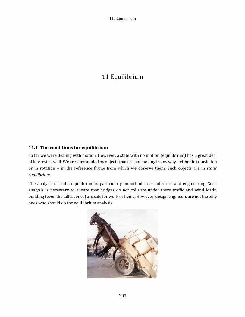
11. Equilibrium
203
11 Equilibrium
11.1 The conditions for equilibrium
So far we were dealing with motion. However, a state with no motion (equilibrium) has a great deal
of interest as well. We are surrounded by objects that are not moving in any way – either in translation
or in rotation – in the reference frame from which we observe them. Such objects are in static
equilibrium.
The analysis of static equilibrium is particularly important in architecture and engineering. Such
analysis is necessary to ensure that bridges do not collapse under there traffic and wind loads,
building (even the tallest ones) are safe for work or living. However, design engineers are not the only
ones who should do the equilibrium analysis.

11.1 The conditions for equilibrium
204
The theory of equilibrium is based on Newton’s laws of motion. A particle is in equilibrium, whenever
the vector sum of all forces acting on it is zero
�⃗�𝑛𝑒𝑡 = 0.
For extended bodies this condition is not enough because they have a tendency to rotate. Therefore
for extended objects the sum of torques about any point must be zero
𝜏𝑛𝑒𝑡 = 0.
Therefore, the analysis of equilibrium is based on these two conditions. Despite the equations look
awfully simple, applications to real problems can be challenging, and quite often require using
computers for solving large system of equations.
Thus, the two requirements for a body to be in equilibrium are follows
These requirements obviously hold for static equilibrium. They also hold for the more general
equilibrium in which total linear and angular momenta are constant but not zero. In the special case
of static equilibrium, which is the main subject of this chapter, the object is at rest and so has no linear
or angular speed (that is, 𝑣𝑐𝑚 = 0, 𝜔 = 0).
The equilibrium conditions, as vector equations, can be written in the component form, one for each
direction of the coordinate axis.
Balance of forces Balance of torques
𝐹𝑛𝑒𝑡.𝑥 = 0 𝜏𝑛𝑒𝑡,𝑥 = 0
𝐹𝑛𝑒𝑡,𝑦 = 0 𝜏𝑛𝑒𝑡,𝑦 = 0
𝐹𝑛𝑒𝑡,𝑧 = 0 𝜏𝑛𝑒𝑡,𝑧 = 0
In introductory physics classes we normally consider situations in which the forces that act on the
body are in xy-plane. That means that the only torques that act on the body can cause rotation around
an axis parallel to the z-axis. Thus we eliminate one force equation, and two torques equations form
the component equations, leaving
1. The vector sum of all the external forces that act on the body, must be zero
�⃗�𝑛𝑒𝑡 = ∑ �⃗�𝑖 = 0 (11.1)
2. The vector sum of all the external torques that act on the body, measured about ANY possible
point, must be zero
𝜏𝑛𝑒𝑡 = ∑ 𝜏𝑖 = 0 (11.2)

11. Equilibrium
205
𝐹𝑛𝑒𝑡,𝑥 = 0 (balance of forces along 𝑥) 𝐹𝑛𝑒𝑡,𝑦 = 0 (balance of forces along 𝑦)
𝜏𝑛𝑒𝑡,𝑧 = 0 (balance of torques around 𝑧) (11.3)
Here 𝜏𝑛𝑒𝑡,𝑧 is the net torque that the external forces produce either around z-axis or about any axis
parallel to it.
If an object is in translational equilibrium and if the net torque is zero about one axis, then the net
torque must also be zero about any other axis. The axis can be inside or outside the borders of the
object. Consider an object being acted on by several forces
�⃗�𝑛𝑒𝑡 = �⃗�1 + �⃗�2 + �⃗�3 + ⋯ = 0
Let 𝑟1 is the point of application of �⃗�1 relative to some point 𝑂, 𝑟2 is the point of application of �⃗�2
relative to the same point 𝑂 and so on. Then, the net torque about an axis through 𝑂 is
𝜏𝑛𝑒𝑡 = 𝑟1 × �⃗�1 + 𝑟2 × �⃗�2 + ⋯
Now consider another arbitrary point 𝑂′ having a position vector 𝑟′ relative to O. Then, the point of
application of �⃗�1 relative to 𝑂′ is identified by the vector 𝑟1 − 𝑟′. Likewise we can write for other forces
�⃗�2, �⃗�3 … Therefore, the net torque about an axis through 𝑂′ is
𝜏𝑛𝑒𝑡 = (𝑟1 − 𝑟′) × �⃗�1 + (𝑟2 − 𝑟′) × �⃗�2 + ⋯ = 𝑟1 × �⃗�1 + 𝑟2 × �⃗�2 + ⋯ − 𝑟′(�⃗�1 + �⃗�2 + ⋯ )
Because the net force is assumed to be zero (given that the object is in translational equilibrium), the
last term vanishes, and we see that the torque about 𝑂′ is equal to the torque about 𝑂. Hence, if an
object is in translational equilibrium and the net torque is zero about one point, then the net torque
must be zero about any other point.
There are many interesting problems when an object is in rotational equilibrium but not in
translational (an accelerating car, when the center of gravity is above the road). It is still possible to
solve such problems but the conditions for equilibrium are different. In this case we deal with
mechanics of non-inertial frames. This subject is commonly considered in courses of theoretical
classical mechanics. Here we only show a way to approach such problems. For example, for
translational motion with acceleration along 𝑥 we have
𝐹𝑛𝑒𝑡,𝑥 = 𝑚𝑎 (motion with acceleration along 𝑥)
𝐹𝑛𝑒𝑡,𝑦 = 0 (balance of forces along 𝑦)
𝜏𝑛𝑒𝑡,𝑧 = 0 (balance of torques around 𝑧)
Then we face a careful choice for a rotational axis because �⃗�𝑛𝑒𝑡 ≠ 0. Normally such point is located at
the center of mass (see example 11-9, 11-10).

11.2 The center of gravity
206
11.2 The center of gravity
The gravitational force on an extended body is the vector sum of the gravitational forces acting on the
individual elements (the atoms) of the body. Instead of considering all those individual elements, we
can say: The gravitational force �⃗�𝑔 on a body effectively acts at a single point, called the center of
gravity of the body. Here the word "effectively" means that if the forces on the individual elements
were somehow turned off and force �⃗�𝑔 at the center of gravity were turned on, the net force and the
net torque (about any point) acting on the body would not change.
First we review the definition for the center of mass (see section 8.3) for a group of particles in (𝑥, 𝑦)
plane with masses 𝑚1, 𝑚2, … and coordinates (𝑥1, 𝑥2, … ), (𝑦1, 𝑦2, … ) the center of mass is given
𝑥𝑐𝑚 =𝑚1𝑥1 + 𝑚2𝑥2 + 𝑚3𝑥3 + ⋯
𝑚1 + 𝑚2 + 𝑚3 + ⋯
𝑦𝑐𝑚 =𝑚1𝑦1 + 𝑚2𝑦2 + 𝑚3𝑦3 + ⋯
𝑚1 + 𝑚2 + 𝑚3 + ⋯
We wish to locate the center of gravity (𝑥𝑐𝑔, 𝑦𝑐𝑔), the point at which application of the single
gravitational force 𝑀�⃗� (where 𝑀 = 𝑚1 + 𝑚2 + ⋯ is the total mass of the object) has the same effect
as does the combined effect of all the individual gravitational forces 𝑚𝑖�⃗�𝑖. Let’s proceed with the
𝑥 coordinate (extension for the 𝑦 coordinate is trivial), then
(𝑚1𝑔1 + 𝑚2𝑔2 + ⋯ )𝑥𝑐𝑔 = 𝑚1𝑔1𝑥1 + 𝑚2𝑔2𝑥2 + ⋯
If we assume uniform 𝑔 over the object (as is usually the case), then
𝑥𝑐𝑔 = 𝑥𝑐𝑚 =𝑚1𝑥1 + 𝑚2𝑥2 + 𝑚3𝑥3 + ⋯
𝑚1 + 𝑚2 + 𝑚3 + ⋯ (11.4)
We see that the center of gravity is located at the center of mass as long as the object is in a uniform
gravitational field. This is approximately true for everyday objects because �⃗� varies only a little along
Earth's surface and decreases in magnitude only slightly with altitude.
Let’s show that the net torque acting on a body can be written as if all the gravitation force is applied
to the center of mass (when �⃗� is the same for all elements of a body).
We consider the individual elements of the body of mass M, and one of its elements, of mass 𝑚𝑖. A
gravitational force acts on each such element and is equal to �⃗�𝑔𝑖 = 𝑚𝑖�⃗�. Each such force produces a
torque on a single element about the origin 𝜏𝑖 = 𝑟𝑖 × 𝑚𝑖�⃗�. The net torque on all the elements of the
body is then
𝜏𝑛𝑒𝑡 = ∑ 𝜏𝑖 = ∑ 𝑟𝑖 × 𝑚𝑖�⃗� = ∑ 𝑚𝑖𝑟𝑖 × �⃗�
Next we divide and multiple this by the total mass of the body 𝑀 = ∑ 𝑚𝑖
𝜏𝑛𝑒𝑡 =1
𝑀∑ 𝑚𝑖𝑟𝑖 × 𝑀�⃗�

11. Equilibrium
207
Using the definition for the center of mass
𝑟𝑐𝑚 =1
𝑀∑ 𝑚𝑖𝑟𝑖
we finally can write
𝜏𝑛𝑒𝑡 = 𝑟𝑐𝑚 × 𝑀�⃗� = 𝑟𝑐𝑚 × �⃗�𝑔. (11.5)
So, the total gravitational torque is the same as though the total gravitational force were acting on the
position of the center of mass, which we also call the center of gravity.
Finding the center of gravity (or the center of mass) can be challenging for bodies of complex shapes.
However, the center of gravity of a homogeneous sphere, cube, circular sheet, or rectangular plate is
at its geometric center. Symmetry considerations can help with more complex shapes when we
sometimes can locate the center of gravity by thinking of the body as being made of symmetrical
pieces.
11.3 Few more words
A body in static equilibrium, if left undisturbed, will undergo no translational or rotational
acceleration since the sum of all the forces and the sum of all the torques acting on it are zero.
However, if the object is displaced slightly, three different outcomes are possible: (1) the object
returns to its original position, in which case it is said to be in stable equilibrium; (2) the object moves
even farther from its original position, in which case it is said to be in unstable equilibrium; or (3) the
object remains in its new position, in which case it is said to be in neutral equilibrium.
Quite often we are interested in maintaining stable equilibrium or balance, as we sometimes say. In
general, an object whose center of gravity is below its point of support, such as a ball on a string, will
be in stable equilibrium. If the center of gravity is above the base of support, we have a more
complicated situation. Consider a standing refrigerator If it is tipped slightly, it will return to its
original position due to the torque on it. But if it is tipped too
far, it will fall over. The critical point is reached when the
center of gravity is no longer above the base of support. In
general, a body whose center of gravity is above its base of
support will be stable if a vertical line projected downward
from the center of gravity falls within the base of support. This
is because the normal force upward on the object (which balances out gravity) can be exerted only
within the area of contact, so that if the force of gravity acts beyond this area, a net torque will act to
topple the object. Stability, then, can be relative. A brick lying on its widest face is more stable than a
brick standing on its end, for it will take more of an effort to tip it over.
Standard physics textbooks usually offer two-dimensional problems in (𝑥, 𝑦) plane. Then we have
only three independent equations for equilibrium, namely two balance of forces equations and one
balance of torques equations about a given rotational axis. However, in real life applications we often
have more unknowns than equations. Consider also an unsymmetrically loaded car. What are the

11.4 Statically undetermined systems
208
forces-all different on the four tires? Again, we cannot find them because we have only three
independent equations with which to work. Similarly, we can solve an equilibrium problem for a table
with three legs but not for one with four legs. Problems like these, in which there are more unknowns
than equations, are called indeterminate. Yet solutions to indeterminate problems exist in the real
world. What is eluding us in our efforts to find the individual forces by solving equations? The
problem is that we have assumed-without making a great point of it that the bodies to which we apply
the equations of static equilibrium are perfectly rigid. By this we mean that they do not deform when
forces are applied to them. Strictly, there are no such bodies. The tires of the car, for example, deform
easily under load until the car settles into a position of static equilibrium. To solve such indeterminate
equilibrium problems, we must supplement equilibrium equations with some knowledge of elasticity,
the branch of physics that describes how real bodies deform when forces are applied to them.
11.4 Statically undetermined systems
In this chapter we consider absolutely rigid bodies, no deformations under stress. However, such
ideal picture is not always a realistic model. Let us consider a rigid beam on two supports and find
forces on the beam from the supports.
The conditions of equilibrium
𝐹1 + 𝐹2 − 𝑚𝑔 = 0
𝐹2𝐿 −𝑚𝑔𝐿
2= 0
Where 𝐿 is the length of the beam. Solving the system of equations gives 𝐹1 = 𝐹2 = 𝑚𝑔 2⁄ . In this
case the model of absolutely rigid body works well.
However, a problem about distribution of weight of a rigid beam between three supports cannot be
solved since we still have two equations for the equilibrium but three unknowns.
𝐹1 + 𝐹2 + 𝐹3 − 𝑚𝑔 = 0
𝐹2𝐿 + 𝐹3𝑥 −𝑚𝑔𝐿
2= 0

11. Equilibrium
209
Mechanical systems, like a beam on three supports, are statically undetermined. The same situation
occurs in equilibrium of a rigid table on a horizontal surface. The problem can be solved for a three
leg table but it is statically undetermined for four or more leg tables. Sure, a real beam and a real
four leg table have a very specific distribution of their weights. The uncertainty comes from an
approximation to consider objects (a beam, a table) as ideally rigid ones. A more accurate model for
a beam should include deformation, or the beam bends under its own weight.
We need to take into account deformation of objects to find unique solutions.
11.5 Few guidelines for solving most common problems in “Equilibrium”
Three dimensional rigid body is a system with six “degrees of freedom” since it can move in three
directions and rotate about three axis. In this chapter we consider two dimensional world, when a
body is flat and located in 𝑥𝑦 −plane, and it can only rotate about 𝑧 −axis. Then there are three
degrees of freedom left, with three equations with conditions for static equilibrium in (𝑥, 𝑦) plane.
𝐹𝑛𝑒𝑡,𝑥 = 0 (balance of forces along 𝑥)
𝐹𝑛𝑒𝑡,𝑦 = 0 (balance of forces along 𝑦)
𝜏𝑛𝑒𝑡,𝑧 = 0 (balance of torques around 𝑧).
Problem solving:
1. You must always draw a free-body diagram showing all the forces acting on the selected body.
2. While choosing the reference point for calculating torques is completely arbitrary, once
selected, the same point must be used to calculate all torques on a body. A wise choice can
considerably simplify your calculations. For example, you can reduce the number of
unknowns by choosing the axis so that one of the unknown forces passes through the axis;
then this force will produce zero torque and so will not appear in the equation.
3. Remember that torque has a direction (positive for counterclockwise “rotation” and negative
for clockwise one).
4. You always need as many equations as you have unknowns. For more complicated problems
you may need to computer torques with respect to two or more axes to obtain enough
equations.
5. Using the component form is much more efficient way to calculate torques.
There is a group of problems in static equilibrium that is called as “balance” problems. Examples of
such problems include: two children on a seesaw, a person walking along a plank extended beyond a
support area. Quite often such problems can be easily solved by calculating the position of the center

11.5 Few guidelines for solving most common problems in “Equilibrium”
210
of gravity instead of dealing with forces and torques. Remember that in general, a body whose center
of gravity is above its base of support will be stable if a vertical line projected downward from the
center of gravity falls within the base of support. The critical point is reached when the center of
gravity is no longer above the base of support.
A quick note on calculating torque (again)
𝜏 = 𝑟 × �⃗�
1. Using angles
𝜏 = 𝑟𝐹 sin 𝜃 = 𝑟𝐹⊥ = 𝑟⊥𝐹
As you probably see using angles may need more steps. Namely
the angle between vectors (counting from 𝑟 to �⃗�) on this diagram
is 900 − 𝜃. Then
𝜏 = 𝑟𝐹 sin 𝜃 = 𝑟𝐹 sin(900 − 𝜃)
Since sin(900 − 𝜃) = cos 𝜃
𝜏 = 𝑟𝐹 sin(900 − 𝜃) = 𝑟 cos 𝜃 𝐹 = 𝑥𝐹
2. Using components in 𝑥𝑦 −plane we have
𝜏𝑧 = 𝑟𝑥𝐹𝑦 − 𝑟𝑦𝐹𝑥.
This way is much more straightforward. For the diagram you immediately get 𝜏𝑧 = 𝑥𝐹.
The component form is invaluable for arbitrary orientations of vectors 𝑟 and �⃗� relative to the
coordinate system. It also provides you with a proper sign (positive or negative) for torques.

11. Equilibrium
211
11.6 Examples
Example 11-1
A uniform beam, of length 𝐿 and mass 𝑚 is at rest with its ends on two scales. A uniform block, with
mass 𝑀, is at rest on the beam, with its center a distance 𝑥 from the beam’s left end. What do the scales
read?
SOLUTION:
1. Physics – static equilibrium
2. The basic equations
𝐹𝑛𝑒𝑡,𝑥 = 0 (𝑏𝑎𝑙𝑎𝑛𝑐𝑒 𝑜𝑓 𝑓𝑜𝑟𝑐𝑒𝑠)
𝐹𝑛𝑒𝑡,𝑦 = 0 (𝑏𝑎𝑙𝑎𝑛𝑐𝑒 𝑜𝑓 𝑓𝑜𝑟𝑐𝑒𝑠)
𝜏𝑛𝑒𝑡,𝑧 = 0 (𝑏𝑎𝑙𝑎𝑛𝑐𝑒 𝑜𝑓 𝑡𝑜𝑟𝑞𝑢𝑒𝑠).
3. We choose the beam as the object of interest
(choosing the block does not help to find the forces on
the scales). The free-body diagram shows all forces
acting on the beam.
The first condition of equilibrium (balance of forces)
for the y-direction (there are no forces acting along x-
direction and 𝐹𝑛𝑒𝑡,𝑥 provides no information)
𝐹𝑛𝑒𝑡,𝑦 = 𝐹1 + 𝐹2 − 𝑀𝑔 − 𝑚𝑔 = 0
For the second condition we need to choose a rotational axis perpendicular to the plane xy. Let’s
choose it through the left end of the beam. Using the component form for calculating torques we get
𝜏𝑧 = 0𝐹1 − 𝑥𝑀𝑔 −𝐿
2𝑚𝑔 + 𝐿𝐹2 = 0
4. Now we have a system of two equations with two unknowns
𝐹1 + 𝐹2 − 𝑀𝑔 − 𝑚𝑔 = 0
−𝑥𝑀𝑔 −𝐿
2𝑚𝑔 + 𝐿𝐹2 = 0
Since the second equation (balance of torques) has only one unknown we can solve it immediately
𝐹2 =𝑥
𝐿𝑀𝑔 +
1
2𝑚𝑔
With this solution we can solve the first equation to find the first force
𝐹1 = −𝐹2 + 𝑀𝑔 + 𝑚𝑔 = −𝑥
𝐿𝑀𝑔 −
1
2𝑚𝑔 + 𝑀𝑔 + 𝑚𝑔 = (1 −
𝑥
𝐿) 𝑀𝑔 +
1
2𝑚𝑔
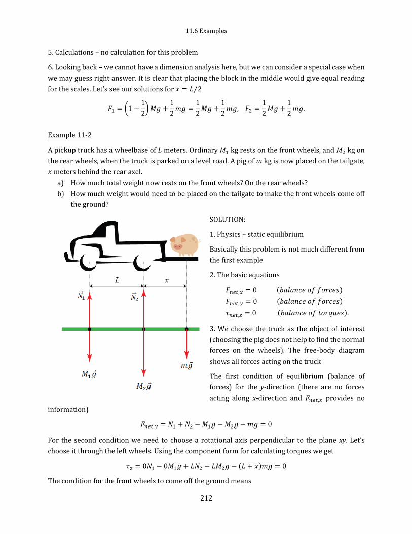
11.6 Examples
212
5. Calculations – no calculation for this problem
6. Looking back – we cannot have a dimension analysis here, but we can consider a special case when
we may guess right answer. It is clear that placing the block in the middle would give equal reading
for the scales. Let’s see our solutions for 𝑥 = 𝐿 2⁄
𝐹1 = (1 −1
2) 𝑀𝑔 +
1
2𝑚𝑔 =
1
2𝑀𝑔 +
1
2𝑚𝑔, 𝐹2 =
1
2𝑀𝑔 +
1
2𝑚𝑔.
Example 11-2
A pickup truck has a wheelbase of 𝐿 meters. Ordinary 𝑀1 kg rests on the front wheels, and 𝑀2 kg on
the rear wheels, when the truck is parked on a level road. A pig of 𝑚 kg is now placed on the tailgate,
𝑥 meters behind the rear axel.
a) How much total weight now rests on the front wheels? On the rear wheels?
b) How much weight would need to be placed on the tailgate to make the front wheels come off
the ground?
SOLUTION:
1. Physics – static equilibrium
Basically this problem is not much different from
the first example
2. The basic equations
𝐹𝑛𝑒𝑡,𝑥 = 0 (𝑏𝑎𝑙𝑎𝑛𝑐𝑒 𝑜𝑓 𝑓𝑜𝑟𝑐𝑒𝑠)
𝐹𝑛𝑒𝑡,𝑦 = 0 (𝑏𝑎𝑙𝑎𝑛𝑐𝑒 𝑜𝑓 𝑓𝑜𝑟𝑐𝑒𝑠)
𝜏𝑛𝑒𝑡,𝑧 = 0 (𝑏𝑎𝑙𝑎𝑛𝑐𝑒 𝑜𝑓 𝑡𝑜𝑟𝑞𝑢𝑒𝑠).
3. We choose the truck as the object of interest
(choosing the pig does not help to find the normal
forces on the wheels). The free-body diagram
shows all forces acting on the truck
The first condition of equilibrium (balance of
forces) for the y-direction (there are no forces
acting along x-direction and 𝐹𝑛𝑒𝑡,𝑥 provides no
information)
𝐹𝑛𝑒𝑡,𝑦 = 𝑁1 + 𝑁2 − 𝑀1𝑔 − 𝑀2𝑔 − 𝑚𝑔 = 0
For the second condition we need to choose a rotational axis perpendicular to the plane xy. Let’s
choose it through the left wheels. Using the component form for calculating torques we get
𝜏𝑧 = 0𝑁1 − 0𝑀1𝑔 + 𝐿𝑁2 − 𝐿𝑀2𝑔 − (𝐿 + 𝑥)𝑚𝑔 = 0
The condition for the front wheels to come off the ground means

11. Equilibrium
213
𝑁1 = 0
Later we will use this condition when we have a solution for 𝑁1
4. Now we have a system of two equations with two unknowns
𝑁1 + 𝑁2 − 𝑀1𝑔 − 𝑀2𝑔 − 𝑚𝑔 = 0
𝐿𝑁2 − 𝐿𝑀2𝑔 − (𝐿 + 𝑥)𝑚𝑔 = 0
Since the second equation (balance of torques) has only one unknown we can solve it immediately
𝑁2 = 𝑀2𝑔 + (1 +𝑥
𝐿) 𝑚𝑔
With this solution we can solve the first equation to find the first force
𝑁1 = −𝑁2 + 𝑀1𝑔 + 𝑀2𝑔 + 𝑚𝑔 = −𝑀2𝑔 − (1 +𝑥
𝐿) 𝑚𝑔 + 𝑀1𝑔 + 𝑀2𝑔 + 𝑚𝑔 = 𝑀1𝑔 −
𝑥
𝐿𝑚𝑔
from 𝑁1 = 0
𝑁1 = 𝑀1𝑔 −𝑥
𝐿𝑚𝑔 = 0
follows
𝑚 = 𝑀1
𝐿
𝑥
With so heavy pig the front wheels will come off the ground. Let’s note that the large 𝑥 the fewer load
needed on the tailgate to have the front wheels off the ground.
5. Calculations – no calculation for this problem
6. Looking back – we cannot have a dimension analysis here, but we can consider a special case when
we may guess right answer. It is clear that without the pig and for 𝑀1 = 𝑀2 = 𝑀 we should expect the
same normal force acting on both front and rear wheels.
𝑁1 = 𝑀1𝑔 = 𝑀𝑔, 𝑁2 = 𝑀2𝑔 = 𝑀𝑔.
We got it right.
Method II for question b).
By the way, the second question is an equilibrium question. It can be easily answered by calculating
the position for the center of gravity. Let’s choose the position of the rear wheels as an origin. Then
the center of gravity of the systems is
𝑥𝑐𝑔 =−𝑀1𝐿 + 𝑀20 + 𝑚𝑥
𝑀1 + 𝑀2 + 𝑚
The critical point is reached when the center of gravity is just above the rear wheels or 𝑥𝑐𝑔 = 0. Then
we have 𝑀1𝐿 = 𝑚𝑥, or 𝑚 = 𝑀1𝐿 𝑥⁄ , or this the same result that we got using forces and torques.

11.6 Examples
214
Example 11-3
A long uniform wooden plank of length L=9.0 m
and mass of M=100.0 kg rests on a deck of a ship.
Only two thirds of the plank is on the deck. How far
from the edge of the ship can Popeye of mass m=60
kg go on the hanging side of the plank if the plank
is to remain at rest?
Assume that the plank does not slide back as
Popeye goes forward
SOLUTION:
1. Physics – static equilibrium, balance problem
2. The basic equations for equilibrium
𝐹𝑛𝑒𝑡,𝑥 = 0 (𝑏𝑎𝑙𝑎𝑛𝑐𝑒 𝑜𝑓 𝑓𝑜𝑟𝑐𝑒𝑠)
𝐹𝑛𝑒𝑡,𝑦 = 0 (𝑏𝑎𝑙𝑎𝑛𝑐𝑒 𝑜𝑓 𝑓𝑜𝑟𝑐𝑒𝑠)
𝜏𝑛𝑒𝑡,𝑧 = 0 (𝑏𝑎𝑙𝑎𝑛𝑐𝑒 𝑜𝑓 𝑡𝑜𝑟𝑞𝑢𝑒𝑠).
For balance problems we calculate the center of gravity
𝑥𝑐𝑔 = 𝑥𝑐𝑚 =𝑚1𝑥1 + 𝑚2𝑥2 + 𝑚3𝑥3 + ⋯
𝑚1 + 𝑚2 + 𝑚3 + ⋯
3. We choose the wooden plank as the object of interest. The free-body diagram shows all forces acting
on the plank
Method I: using the center of gravity. Choosing the
red dot as the origin (𝑥 = 0) we have
𝑥𝑐𝑔 =−𝑀𝑥𝑐 + 𝑚𝑥
𝑀 + 𝑚
The critical point is reached when the center of
gravity is just above the edge of the ship (the red
dot). Then from 𝑥𝑐𝑔 = 0 one has
𝑥 = 𝑥𝐶
𝑀
𝑚
Method II: general approach to equilibrium
problems. The problem looks very similar the first
two problems. However, there is something new.
Where is the normal force applied? Should it be at
the same x position as the gravity on the plank? If we place the normal vector at the location of the
center of gravity, then we would get rotation from 𝑚�⃗� around the center of gravity!

11. Equilibrium
215
One may say, well I expect the normal force be at the edge of the ship when Popeye is going to start
falling.
Let’s avoid any guesses and proceed with equations.
The first condition of equilibrium (balance of forces) for the y-direction (there are no forces acting
along x-direction and 𝐹𝑛𝑒𝑡,𝑥 provides no information).
𝐹𝑛𝑒𝑡,𝑦 = 𝑁 − 𝑀𝑔 − 𝑚𝑔 = 0
For the second condition we need to choose a rotational axis perpendicular to the plane xy. Let’s
choose it through the “red” point (the edge of the ship) as the origin for the coordinate system. Using
the component form for calculating torques we get
𝜏𝑧 = 𝑥𝐶𝑀𝑔 − 𝑥𝑁𝑁 − 𝑥𝑚𝑔 = 0
4. Now we have a system of two equations with two unknowns (𝑁 and 𝑥𝑁) for some position 𝑥.
𝑁 − 𝑀𝑔 − 𝑚𝑔 = 0
𝑥𝐶𝑀𝑔 − 𝑥𝑁𝑁 − 𝑥𝑚𝑔 = 0
Solving for the unknowns
𝑁 = 𝑀𝑔 + 𝑚𝑔
𝑥𝑁 =𝑥𝐶𝑀𝑔 − 𝑥𝑚𝑔
(𝑀 + 𝑚)𝑔=
𝑋𝐶𝑀 − 𝑥𝑚
𝑀 + 𝑚
As we can see the location of the normal force is not at the center of gravity!
Now, when the position of the normal force at the edge of the ship, then this is where a delicate
balance happens, any more step and Popeye goes swimming (normal force cannot act from the air, it
has to be from a surface). Thus, the balance condition is 𝑥𝑁 = 0. From this condition
𝑥𝑁 =𝑥𝐶𝑀 − 𝑥𝑚
𝑀 + 𝑚= 0
we get
𝑥 = 𝑥𝐶
𝑀
𝑚
5. Calculations
Note that from the condition for the plan’s position follows that 𝑥𝐶 = (1 2⁄ − 1 3⁄ )𝐿 = 𝐿 6⁄
𝑥 =1
69 𝑚
100 𝑘𝑔
60 𝑘𝑔= 2.5 𝑚
6. Looking back – correct dimensions.
Let’s consider a special case when we may guess right answers. If our solution is able to reproduce
our special case consideration then we probably have a correct solution.

11.6 Examples
216
Without Popeye the position of the normal force should be at the same horizontal position as the
gravitational force. For 𝑚 = 0 we have 𝑥𝑁 = 𝑥𝐶 . Correct.
By the way, using the “center-of-gravity” approach (method I) to this balance problem produced the
answer in just few equations.
Example 11-4
A crane is mounted on a truck. The mass of the truck is 𝑀 = 5,000 𝑘𝑔, the width of the truck (the
distance between outer sides of the tires) is 𝐷 = 3.2 𝑚, the center of mass of the truck (with the crane)
is ℎ = 2 𝑚 above the ground, the end of the boom of the crane is extended 𝐿 = 5 𝑚 from the center of
the gravity of the truck (assume that the mass of the boom is much less than the mass of the truck).
What is the maximum mass of a load the crane can lift without going overturned?
SOLUTION:
1. Physics – static equilibrium, balance problem
2. The basic equations for equilibrium
𝐹𝑛𝑒𝑡,𝑥 = 0 (𝑏𝑎𝑙𝑎𝑛𝑐𝑒 𝑜𝑓 𝑓𝑜𝑟𝑐𝑒𝑠)
𝐹𝑛𝑒𝑡,𝑦 = 0 (𝑏𝑎𝑙𝑎𝑛𝑐𝑒 𝑜𝑓 𝑓𝑜𝑟𝑐𝑒𝑠)
𝜏𝑛𝑒𝑡,𝑧 = 0 (𝑏𝑎𝑙𝑎𝑛𝑐𝑒 𝑜𝑓 𝑡𝑜𝑟𝑞𝑢𝑒𝑠).
the center of gravity
𝑥𝑐𝑔 = 𝑥𝑐𝑚 =𝑚1𝑥1 + 𝑚2𝑥2 + 𝑚3𝑥3 + ⋯
𝑚1 + 𝑚2 + 𝑚3 + ⋯
3. While this problem can be solved using the
equilibrium conditions, it is much easier to approach it as a balance problem. Choosing the origin (𝑥 =
0) at the right side of the truck we have
𝑥𝑐𝑔 =−
𝑀𝑑2 + 𝑚 (𝐿 −
𝐷2)
𝑀 + 𝑚
4. The critical point is reached when the center of gravity is just above the right side of the truck, then
from 𝑥𝑐𝑔 = 0
𝑚 = 𝑀𝐷
2𝐿 − 𝐷
5. Calculations
𝑚 = 5000 𝑘𝑔 3.2 𝑚
2 ∙ 5 𝑚 − 3.2 𝑚= 2352 𝑘𝑔
6. Looking back – we have right dimensions, and the results looks as a credible one.

11. Equilibrium
217
Example 11-5
A safe of mass 𝑀 hanging by a rope from a boom with
dimensions 𝑎 and 𝑏. The boom consists of a hinged beam and
a horizontal cable that connects the beam to a wall. The
uniform beam has a mass 𝑚. The masses of the cable and the
rope are negligible.
a) What is the tension in the cable?
b) Find the magnitude of the net force on the beam from
the hinge.
SOLUTION:
1. Physics – static equilibrium
This problem, unlike the first two, is a two-dimensional problem
2. The basic equations
𝐹𝑛𝑒𝑡,𝑥 = 0 (𝑏𝑎𝑙𝑎𝑛𝑐𝑒 𝑜𝑓 𝑓𝑜𝑟𝑐𝑒𝑠)
𝐹𝑛𝑒𝑡,𝑦 = 0 (𝑏𝑎𝑙𝑎𝑛𝑐𝑒 𝑜𝑓 𝑓𝑜𝑟𝑐𝑒𝑠)
𝜏𝑛𝑒𝑡,𝑧 = 0 (𝑏𝑎𝑙𝑎𝑛𝑐𝑒 𝑜𝑓 𝑡𝑜𝑟𝑞𝑢𝑒𝑠).
3. We choose the beam as the object of interest (see why not
the cable or the rope?)
Let’s note that 𝑇𝑟 = 𝑀𝑔 from the equilibrium condition for the
safe. We will use it in a moment.
The balance of forces
𝐹𝑛𝑒𝑡,𝑥 = 𝐹ℎ − 𝑇𝑐 = 0
𝐹𝑛𝑒𝑡,𝑦 = 𝐹𝑣 − 𝑚𝑔 − 𝑀𝑔 = 0
For the balance of torques we need to choose a rotational axis
perpendicular to the plane xy. Let’s choose it through the hinge. Thus we will have fewer unknowns
in our equation.
Using the component form for calculating torques we get
𝜏𝑧 = −𝑏
2𝑚𝑔 − 𝑏𝑀𝑔 + 𝑎𝑇𝑐 = 0
Using the component from makes it much easier to calculate the torques. Otherwise you would be
wrestling with the angles.
4. Now we have a system of three equations with three unknowns (𝑇𝑐 , 𝐹ℎ , 𝐹𝑣)
𝐹ℎ − 𝑇𝑐 = 0
𝐹𝑣 − 𝑚𝑔 − 𝑀𝑔 = 0

11.6 Examples
218
−𝑏
2𝑚𝑔 − 𝑏𝑀𝑔 + 𝑎𝑇𝑐 = 0
The last equation immediately gives the tension in the cable
𝑇𝑐 =𝑏
2𝑎𝑚𝑔 +
𝑏
𝑎𝑀𝑔 =
𝑏
𝑎(
1
2𝑚 + 𝑀) 𝑔
Then the horizontal and vertical components of the force on the hinge
𝐹ℎ = 𝑇𝑐 =𝑏
𝑎(
1
2𝑚 + 𝑀) 𝑔
𝐹𝑣 = (𝑚 + 𝑀)𝑔
The magnitude of the net force on the beam from the hinge
𝐹ℎ𝑖𝑛𝑔𝑒 = √𝐹ℎ2 + 𝐹𝑣
2
5. Calculations – no calculation for this problem
6. Looking back – we cannot have a dimension analysis here, but we can consider a special case when
we may guess right answer.
We can assume that for a vertical beam there is no need for the supporting cable, or if 𝑏 = 0, then
𝑇𝑐 = 0. This is exactly what follows from our general solution
Example 11-6
A sign of mass Ms= 8.0 kg is supported by a uniform m=4.0 kg beam
as shown on the figure. A cat (Tom) of mass Mc=5.0 kg walks slowly
from the wall toward the end of the beam to talk to Jerry (mm= 0.2 kg)
probably about physics of equilibrium.
a) Will the cable break before the cat reaches the end of the
beam, if the cable will break up under tension of 280.0 N?
b) If so, how far from the wall the cat will be when the cable
breaks?
The cable is d=2.0 meters long. It makes 300 degrees with the beam.
Assume that the mass of the cable is negligible.
SOLUTION:
1. Physics – static equilibrium
2. The basic equations
𝐹𝑛𝑒𝑡,𝑥 = 0 (𝑏𝑎𝑙𝑎𝑛𝑐𝑒 𝑜𝑓 𝑓𝑜𝑟𝑐𝑒𝑠)
𝐹𝑛𝑒𝑡,𝑦 = 0 (𝑏𝑎𝑙𝑎𝑛𝑐𝑒 𝑜𝑓 𝑓𝑜𝑟𝑐𝑒𝑠)
𝜏𝑛𝑒𝑡,𝑧 = 0 (𝑏𝑎𝑙𝑎𝑛𝑐𝑒 𝑜𝑓 𝑡𝑜𝑟𝑞𝑢𝑒𝑠).

11. Equilibrium
219
3. We choose the beam as the object of interest
(not the cat, or the mouse or the cable). The beam
is 𝐿 = 𝑑 cos 𝜃 long.
There are two ways to approach the problem.
a. We can place the cat at the end of the beam
(distance 𝐿 from the wall) to see if the cable
breaks under this condition. If it breaks then we
have to solve the problem again to find at what
position 𝑥 of the cat it will happen.
b. Or we can find the tension in the cable having
the cat distance 𝑥 from the wall. Then we use the
condition 𝑇 = 𝑇𝑐𝑟𝑖𝑡𝑖𝑐𝑎𝑙 to find 𝑥𝑐𝑟𝑖𝑡𝑖𝑐𝑎𝑙. If it less than the size of the beam, then the cable will break.
The second way is preferable since we have to solve the problem once.
The balance of forces
𝐹𝑛𝑒𝑡,𝑥 = 𝐹𝑥 − 𝑇 cos 𝜃 = 0
𝐹𝑛𝑒𝑡,𝑦 = 𝐹𝑦 − 𝑀𝑐𝑔 − 𝑚𝑔 − (𝑀𝑠 + 𝑚𝑚)𝑇 sin 𝜃 = 0
Let’s choose the rotational axis at the left end of the beam (thus we will have fewer unknowns in our
equation. Using components the balance of torques is
𝜏𝑧 = −𝑥𝑀𝑐𝑔 −𝐿
2𝑚𝑔 − (𝑀𝑠 + 𝑚𝑚)𝑔 + 𝐿𝑇 sin 𝜃 = 0
(Note that we used here the component equation for torques, namely 𝜏𝑧 = 𝑟𝑥𝐹𝑦 − 𝑟𝑦𝐹𝑥.)
4. We have a system of three equations with three unknowns (𝑥, 𝐹𝑥 , 𝐹𝑦), but we need to find only one
– the distance when the cable will break.
𝐹𝑥 − 𝑇 cos 𝜃 = 0
𝐹𝑦 − 𝑀𝑐𝑔 − 𝑚𝑔 − (𝑀𝑠 + 𝑚𝑚)𝑇 sin 𝜃 = 0
−𝑥𝑀𝑐𝑔 −𝐿
2𝑚𝑔 − 𝐿(𝑀𝑠 + 𝑚𝑚)𝑔 + 𝐿𝑇 sin 𝜃 = 0
With the wise choice of the rotational axis, we have it right in the third equation where we use 𝑇 =
𝑇𝑐𝑟𝑖𝑡𝑖𝑐𝑎𝑙.
𝑥 = 𝐿1
𝑀𝑐(
𝑇𝑐𝑟𝑖𝑡𝑖𝑐𝑎𝑙 sin 𝜃
𝑔−
1
2𝑚 − 𝑀𝑠 − 𝑚𝑚)
5. Calculations are straightforward

11.6 Examples
220
For the given critical tension, the cat should be 1.42 m from the wall to have the cable broken.
However, the beam is 𝐿 = 2.0 𝑚 ∙ cos 300 = 1.73 𝑚. That means that the cable will break before Tom
gets to the end of the beam.
6. Looking back.
Since tension is measured in [N] (where [N]=[m][g]), then we have right units for the distance.
A quick analysis of equation for 𝑥 shows that for heavier cats the critical distance is getting shorter.
If there is no Tom and Jerry (𝑀𝑐 = 0, 𝑚𝑚 = 0), the tension in the cable
𝑇 =1
sin 𝜃(
1
2𝑚 + 𝑀𝑠) 𝑔
Example 11-7
This problem may look a bit challenging but could be a practical one.
Two friends are carrying a 200-kg crate up a flight of
stairs. The crate is L=1.25 m long and w=0.500 m high, and
its center of gravity is at its center. The stairs make a 450
angle with respect to the floor. The crate is also carried at
a 450 angle, so its bottom side is parallel to the slope of the
stairs. If the force each person applies is vertical, what is
the magnitude of each of these forces? Is it better to be the
person above or below on the stairs?
SOLUTION:
1. Physics – static equilibrium.
2. The basic equations
𝐹𝑛𝑒𝑡,𝑥 = 0 (𝑏𝑎𝑙𝑎𝑛𝑐𝑒 𝑜𝑓 𝑓𝑜𝑟𝑐𝑒𝑠)
𝐹𝑛𝑒𝑡,𝑦 = 0 (𝑏𝑎𝑙𝑎𝑛𝑐𝑒 𝑜𝑓 𝑓𝑜𝑟𝑐𝑒𝑠)
𝜏𝑛𝑒𝑡,𝑧 = 0 (𝑏𝑎𝑙𝑎𝑛𝑐𝑒 𝑜𝑓 𝑡𝑜𝑟𝑞𝑢𝑒𝑠).
3. We choose the crate as the object of interest. Here 𝜃 is
the angle that the crate makes with the floor (not with
the flight of stairs. Since this problem involves using
geometry and trigonometry we better have a good set of
notations on our diagram.
The balance of forces
𝐹𝑛𝑒𝑡,𝑥 = 0
𝐹𝑛𝑒𝑡,𝑦 = 𝐹1 + 𝐹2 − 𝑀𝑔 = 0

11. Equilibrium
221
Let’s choose the rotational axis at the lower left end of the crate. Using components ( 𝜏𝑧 = 𝑟𝑥𝐹𝑦 −
𝑟𝑦𝐹𝑥)
the balance of torques is
𝜏𝑧 = −𝑥𝑀𝑔 + 𝐿 cos 𝜃 𝐹2 = 0
4. We have a system of two equations with two unknowns (𝐹1, 𝐹2).
𝐹1 + 𝐹2 − 𝑀𝑔 = 0
−𝑥𝑀𝑔 + 𝐿 cos 𝜃 𝐹2 = 0
Now we need to find 𝑥 in terms of 𝐿, 𝑤, 𝜃. Here geometry + trigonometry come. For the small “orange”
triangle inside the crate we have the same angle 𝜃 as the angle with the floor (do you see why?). Since
we know 𝑏 = 𝑤/2 we can find 𝑎
𝑎 = 𝑏 tan 𝜃 =𝑤
2tan 𝜃
Since 𝑠 + 𝑎 = 𝐿/2
𝑠 =𝐿
2−
𝑤
2tan 𝜃
because 𝑥 = 𝑠 cos 𝜃 we finally get
𝑥 = (𝐿
2−
𝑤
2tan 𝜃) cos 𝜃 =
1
2(𝐿 cos 𝜃 − 𝑤 sin 𝜃)
With this 𝑥 we can write the solution from the balance of torques as
𝐹2 =𝑥𝑀𝑔
𝐿 cos 𝜃=
1
2(
𝐿 cos 𝜃
𝐿 cos 𝜃−
𝑤 sin 𝜃
𝐿 cos 𝜃) 𝑀𝑔 =
1
2(1 −
𝑤
𝐿tan 𝜃) 𝑀𝑔
Then the first force can be found from the balance of forces
𝐹1 = 𝑀𝑔 − 𝐹2 =1
2(1 +
𝑤
𝐿tan 𝜃) 𝑀𝑔
5. Calculations
𝐹1 =1
2(1 +
0.50 𝑚
1.25 𝑚𝐿tan 300) 200 𝑘𝑔 ∙ 9.8 𝑚 𝑠2⁄ = 1372 𝑁
𝐹2 = 1
2(1 −
0.50 𝑚
1.25 𝑚𝐿tan 300) 200 𝑘𝑔 ∙ 9.8 𝑚 𝑠2⁄ = 588 𝑁
It is clear that it is better to be the person above on the stairs. But if you are a good friend you will
probably take the place at the lower end.
6. Looking back.
Let’s consider a special case (or two) when we may guess right answers. If our general solution is able
to reproduce our special case considerations then probably we have a correct general solution.

11.6 Examples
222
It is clear that if the friend were on the floor (then the angle 𝜃 = 0) we should expect equal load for
both. From our general solution it follows for 𝜃 = 0
𝐹1 =1
2𝑀𝑔, 𝐹2 =
1
2𝑀𝑔
What if it was not a crate but a beam (or a log) with negligible width comparing to its length (𝑤 ≪ 𝐿)?
Then we have
𝐹1 =1
2𝑀𝑔, 𝐹2 =
1
2𝑀𝑔
That means that we see the difference if you are on a flight of stairs carrying a wide object. By the way
we can easily find such an angle when the person above on the stairs does not carry anything, or 𝐹2 =
0, thus from
𝐹2 =1
2(1 −
𝑤
𝐿tan 𝜃) 𝑀𝑔 = 0
we have
tan 𝜃 =𝐿
𝑤
(for the given crate this angle is about 680).
Example 11-8
You are trying to move a dresser of mass 𝑀 and dimensions of length 𝐿 and height 𝐻 by pushing it
with a constant velocity by applying a horizontal force 𝐹 a height ℎ above the floor. The coefficient of
kinetic friction between the dresser and the floor is 𝜇. The ground exerts upward normal forces of
magnitudes 𝑁1 and 𝑁2 at the two ends of the dresser.
Find the height about the floor that you can push a dresser before it starts to topple.

11. Equilibrium
223
SOLUTION:
1. Physics – static equilibrium, friction
2. The basic equations
𝐹𝑛𝑒𝑡,𝑥 = 0 (𝑏𝑎𝑙𝑎𝑛𝑐𝑒 𝑜𝑓 𝑓𝑜𝑟𝑐𝑒𝑠)
𝐹𝑛𝑒𝑡,𝑦 = 0 (𝑏𝑎𝑙𝑎𝑛𝑐𝑒 𝑜𝑓 𝑓𝑜𝑟𝑐𝑒𝑠)
𝜏𝑛𝑒𝑡,𝑧 = 0 (𝑏𝑎𝑙𝑎𝑛𝑐𝑒 𝑜𝑓 𝑡𝑜𝑟𝑞𝑢𝑒𝑠).
Friction
𝑓 = 𝜇𝑁
3. The balance of forces
𝐹𝑛𝑒𝑡,𝑥 = 𝐹 − 𝑓1 − 𝑓2 = 𝐹 − 𝜇𝑁1 − 𝜇𝑁2 = 0
𝐹𝑛𝑒𝑡,𝑦 = 𝑁1 + 𝑁2 − 𝑀𝑔 = 0
Let’s choose the rotational axis at the RIGHT end of the
dresser. Using components ( 𝜏𝑧 = 𝑟𝑥𝐹𝑦 − 𝑟𝑦𝐹𝑥)
the balance of torques is
𝜏𝑧 = −ℎ𝐹 − 𝐿𝑁1 +𝐿
2𝑀𝑔 = 0
4. Our system of equations.
𝐹 − 𝜇𝑁1 − 𝜇𝑁2 = 0
𝑁1 + 𝑁2 − 𝑀𝑔 = 0
−ℎ𝐹 − 𝐿𝑁1 +𝐿
2𝑀𝑔 = 0
From the first equation 𝐹 = 𝜇(𝑁1 + 𝑁2). Since 𝑁1 + 𝑁2 = 𝑀𝑔 (from the second equation), the we have
that the force to push with constant velocity is
𝐹 = 𝜇𝑀𝑔
or the net frictional force. With this information, the last equation immediately gives 𝑁1
𝑁1 =1
2𝑀𝑔 −
ℎ
𝐿𝜇𝑀𝑔
and then
𝑁2 = 𝑀𝑔 − 𝑁1 =1
2𝑀𝑔 +
ℎ
𝐿𝜇𝑀𝑔
Let’s note that the left end will lose contact with the floor (𝑁1 = 0) at the moment the dresser begins
to topple. Thus
𝑁1 = 0 =1
2𝑀𝑔 −
ℎ𝑚
𝐿𝜇𝑀𝑔

11.6 Examples
224
where ℎ𝑚 is the maximum height about the floor that you can push a dresser before it starts to topple.
ℎ𝑚 =𝐿
2𝜇
5. No calculations
6. Looking back.
Let’s consider a special case (or two) when we may guess right answers. If our general solution is able
to reproduce our special case considerations then probably we have a correct solution.
It is clear that in absence of friction 𝜇 = 0 𝑎𝑛𝑑 ℎ𝑚 → ∞ there is no way to get a problem with furniture
(but then how could we move furniture if we do not have traction?).
Example 11-9
A car is travelling at a constant speed 𝑣 on a horizontal curved ramp of radius 𝑅 = 100 𝑚. Assume the
height of the car’s center of mass above the ground is ℎ = 1.0 m, and the separation between its wheels
(the axle track or car’s width) is 𝐿 = 1.6 𝑚. The maximum coefficient of static friction between the
tires and the surface of the road is 𝜇𝑠 = 0.9.
a) Find its maximum speed if the car is to negotiate this path without skidding.
b) Find its maximum speed if the car is to negotiate the path without overturning.
SOLUTION:
1. Physics – circular motion with acceleration, friction, rotational equilibrium.
Let’s note that the first question has been answered in example 5-11 (question a), namely, 𝑣𝑚𝑎𝑥 =
√𝜇𝑠𝑔𝑅. However, it is interesting to compare the two solutions, for skidding and overturning, or what
is going to happen first. Now, we concentrate on question b).
2. The basic equations
𝐹𝑛𝑒𝑡,𝑥 =𝑀𝑣2
𝑅 (𝑐𝑒𝑛𝑡𝑟𝑖𝑝𝑒𝑡𝑎𝑙 𝑓𝑜𝑟𝑐𝑒)
𝐹𝑛𝑒𝑡,𝑦 = 0 (𝑏𝑎𝑙𝑎𝑛𝑐𝑒 𝑜𝑓 𝑓𝑜𝑟𝑐𝑒𝑠)
𝜏𝑛𝑒𝑡,𝑧 = 0 (𝑏𝑎𝑙𝑎𝑛𝑐𝑒 𝑜𝑓 𝑡𝑜𝑟𝑞𝑢𝑒𝑠).
Friction 𝑓 = 𝜇𝑁
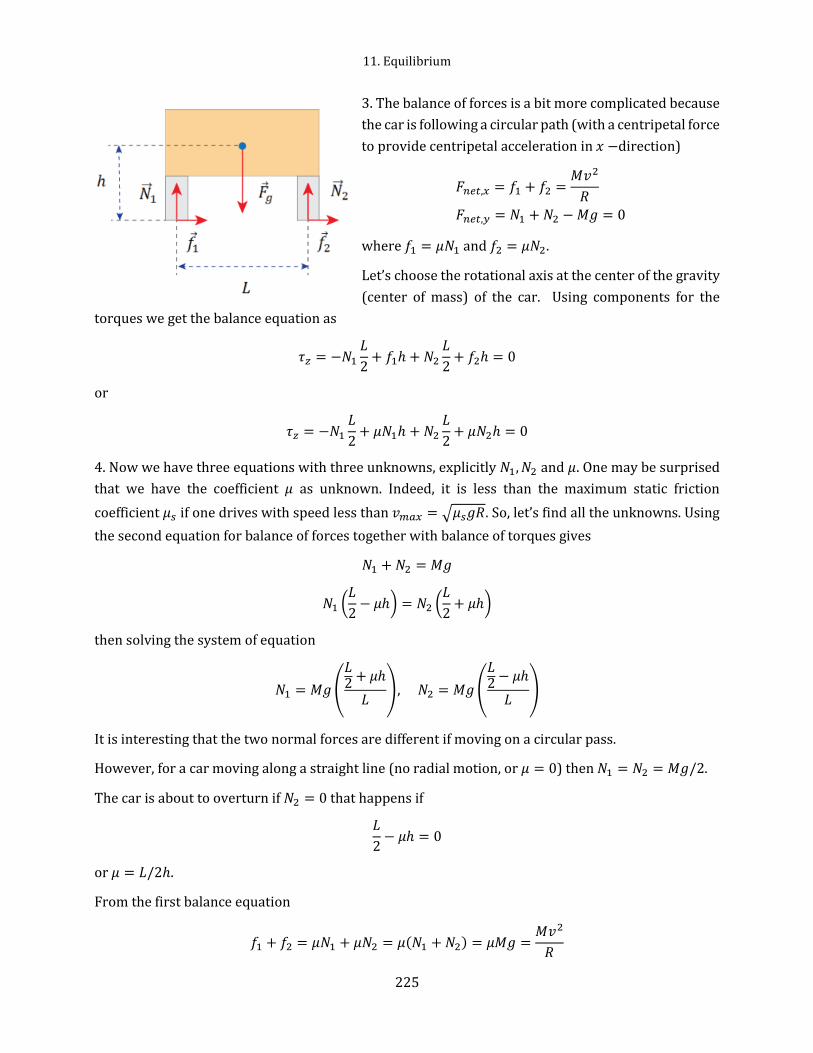
11. Equilibrium
225
3. The balance of forces is a bit more complicated because
the car is following a circular path (with a centripetal force
to provide centripetal acceleration in 𝑥 −direction)
𝐹𝑛𝑒𝑡,𝑥 = 𝑓1 + 𝑓2 =𝑀𝑣2
𝑅
𝐹𝑛𝑒𝑡,𝑦 = 𝑁1 + 𝑁2 − 𝑀𝑔 = 0
where 𝑓1 = 𝜇𝑁1 and 𝑓2 = 𝜇𝑁2.
Let’s choose the rotational axis at the center of the gravity
(center of mass) of the car. Using components for the
torques we get the balance equation as
𝜏𝑧 = −𝑁1
𝐿
2+ 𝑓1ℎ + 𝑁2
𝐿
2+ 𝑓2ℎ = 0
or
𝜏𝑧 = −𝑁1
𝐿
2+ 𝜇𝑁1ℎ + 𝑁2
𝐿
2+ 𝜇𝑁2ℎ = 0
4. Now we have three equations with three unknowns, explicitly 𝑁1, 𝑁2 and 𝜇. One may be surprised
that we have the coefficient 𝜇 as unknown. Indeed, it is less than the maximum static friction
coefficient 𝜇𝑠 if one drives with speed less than 𝑣𝑚𝑎𝑥 = √𝜇𝑠𝑔𝑅. So, let’s find all the unknowns. Using
the second equation for balance of forces together with balance of torques gives
𝑁1 + 𝑁2 = 𝑀𝑔
𝑁1 (𝐿
2− 𝜇ℎ) = 𝑁2 (
𝐿
2+ 𝜇ℎ)
then solving the system of equation
𝑁1 = 𝑀𝑔 (
𝐿2
+ 𝜇ℎ
𝐿), 𝑁2 = 𝑀𝑔 (
𝐿2
− 𝜇ℎ
𝐿)
It is interesting that the two normal forces are different if moving on a circular pass.
However, for a car moving along a straight line (no radial motion, or 𝜇 = 0) then 𝑁1 = 𝑁2 = 𝑀𝑔/2.
The car is about to overturn if 𝑁2 = 0 that happens if
𝐿
2− 𝜇ℎ = 0
or 𝜇 = 𝐿/2ℎ.
From the first balance equation
𝑓1 + 𝑓2 = 𝜇𝑁1 + 𝜇𝑁2 = 𝜇(𝑁1 + 𝑁2) = 𝜇𝑀𝑔 =𝑀𝑣2
𝑅

11.6 Examples
226
or
𝜇 =𝑣2
𝑔𝑅
Using 𝜇 = 𝐿/2ℎ from the above solution gives
𝐿
2ℎ=
𝑣2
𝑔𝑅
𝑣𝑜𝑣𝑒𝑟 = √𝐿
2ℎ𝑔𝑅
where 𝑣𝑜𝑣𝑒𝑟 is the maximum speed a car may have before starting to overturn. By the way, the larger
ℎ the lower the critical 𝑣𝑜𝑣𝑒𝑟 speed (that is the case for SUVs where the ratio 𝐿/2ℎ is lower than for
regular cars).
5. For the given conditions
𝑣𝑚𝑎𝑥 = √𝜇𝑠𝑔𝑅 = √0.9 ∙ 9.8𝑚
𝑠2∙ 100𝑚 = 30 𝑚/𝑠 = 67 𝑚𝑝ℎ
𝑣𝑜𝑣𝑒𝑟 = √𝐿
2ℎ𝑔𝑅 = √
1.6 𝑚
2 ∙ 1 𝑚9.8
𝑚
𝑠2∙ 100𝑚 = 28 𝑚/𝑠 = 63 𝑚𝑝ℎ
6. Looking back.
For the given conditions the care will rather overturn than skid.
Example 11-10
A driver of a car on a horizontal road makes an emergency stop by applying the brakes so that all four
wheels lock and skid along the road. The coefficient of kinetic friction between tires and road is 𝜇 =
0.80. The wheelbase (the separation between the front and rear axles) is 𝐷 = 2.8 𝑚, and the center
of mass of the car is located at distance 𝑑 = 1.2 𝑚 behind the front axle and distance ℎ = 0.90 𝑚
above the road. The car mass is 𝑀 = 1000 𝑘𝑔. Find the magnitude of the normal force on rear wheels
and the normal force on front wheels.
SOLUTION:
1. Physics – motion with translational acceleration, friction, rotational equilibrium. (While the car is
not in translational equilibrium, it is in rotational equilibrium!).
This problem is remarkably similar to example 11-8.
2. The basic equations
𝐹𝑛𝑒𝑡,𝑥 = 𝑀𝑎 (𝑎𝑐𝑐𝑒𝑙𝑒𝑟𝑎𝑡𝑖𝑜𝑛 𝑖𝑛 𝑥 𝑑𝑖𝑟𝑒𝑐𝑡𝑖𝑜𝑛)
𝐹𝑛𝑒𝑡,𝑦 = 0 (𝑏𝑎𝑙𝑎𝑛𝑐𝑒 𝑜𝑓 𝑓𝑜𝑟𝑐𝑒𝑠)
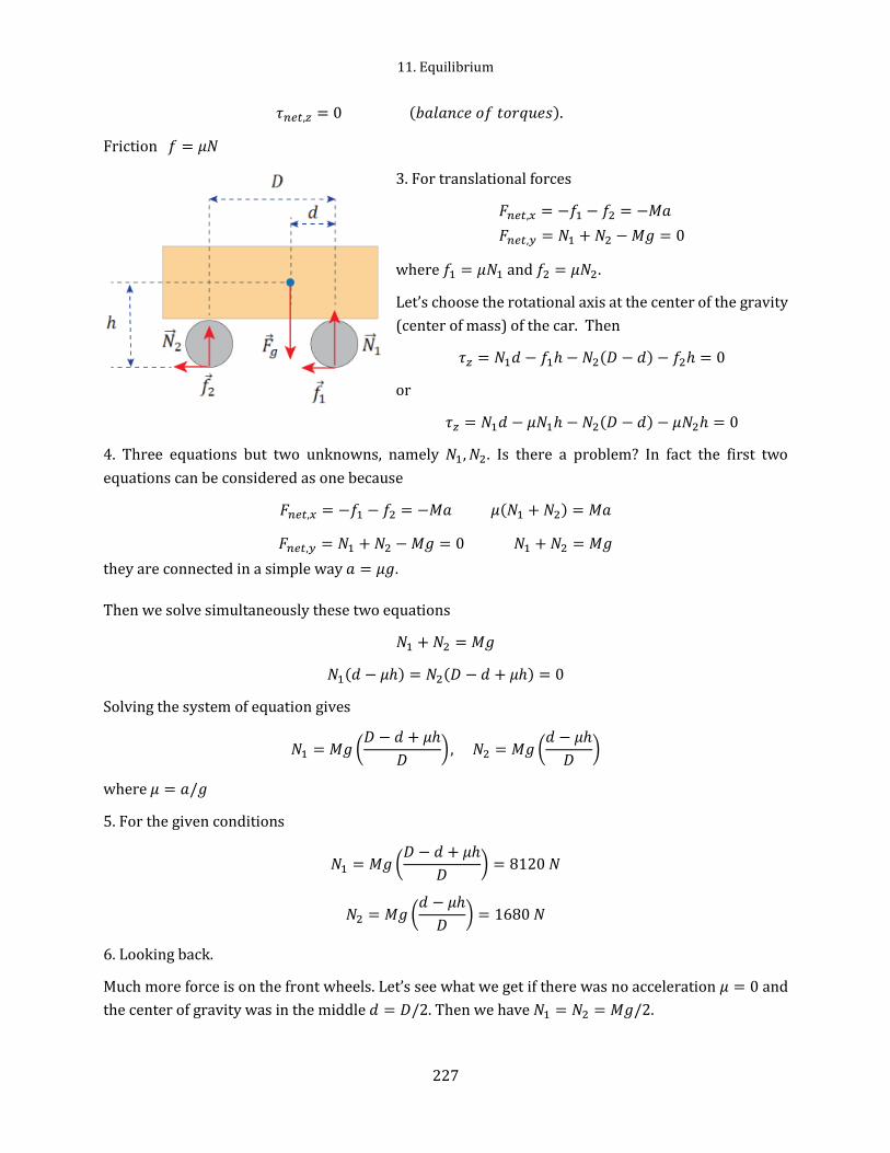
11. Equilibrium
227
𝜏𝑛𝑒𝑡,𝑧 = 0 (𝑏𝑎𝑙𝑎𝑛𝑐𝑒 𝑜𝑓 𝑡𝑜𝑟𝑞𝑢𝑒𝑠).
Friction 𝑓 = 𝜇𝑁
3. For translational forces
𝐹𝑛𝑒𝑡,𝑥 = −𝑓1 − 𝑓2 = −𝑀𝑎
𝐹𝑛𝑒𝑡,𝑦 = 𝑁1 + 𝑁2 − 𝑀𝑔 = 0
where 𝑓1 = 𝜇𝑁1 and 𝑓2 = 𝜇𝑁2.
Let’s choose the rotational axis at the center of the gravity
(center of mass) of the car. Then
𝜏𝑧 = 𝑁1𝑑 − 𝑓1ℎ − 𝑁2(𝐷 − 𝑑) − 𝑓2ℎ = 0
or
𝜏𝑧 = 𝑁1𝑑 − 𝜇𝑁1ℎ − 𝑁2(𝐷 − 𝑑) − 𝜇𝑁2ℎ = 0
4. Three equations but two unknowns, namely 𝑁1, 𝑁2. Is there a problem? In fact the first two
equations can be considered as one because
𝐹𝑛𝑒𝑡,𝑥 = −𝑓1 − 𝑓2 = −𝑀𝑎 𝜇(𝑁1 + 𝑁2) = 𝑀𝑎
𝐹𝑛𝑒𝑡,𝑦 = 𝑁1 + 𝑁2 − 𝑀𝑔 = 0 𝑁1 + 𝑁2 = 𝑀𝑔
they are connected in a simple way 𝑎 = 𝜇𝑔.
Then we solve simultaneously these two equations
𝑁1 + 𝑁2 = 𝑀𝑔
𝑁1(𝑑 − 𝜇ℎ) = 𝑁2(𝐷 − 𝑑 + 𝜇ℎ) = 0
Solving the system of equation gives
𝑁1 = 𝑀𝑔 (𝐷 − 𝑑 + 𝜇ℎ
𝐷), 𝑁2 = 𝑀𝑔 (
𝑑 − 𝜇ℎ
𝐷)
where 𝜇 = 𝑎/𝑔
5. For the given conditions
𝑁1 = 𝑀𝑔 (𝐷 − 𝑑 + 𝜇ℎ
𝐷) = 8120 𝑁
𝑁2 = 𝑀𝑔 (𝑑 − 𝜇ℎ
𝐷) = 1680 𝑁
6. Looking back.
Much more force is on the front wheels. Let’s see what we get if there was no acceleration 𝜇 = 0 and
the center of gravity was in the middle 𝑑 = 𝐷/2. Then we have 𝑁1 = 𝑁2 = 𝑀𝑔/2.
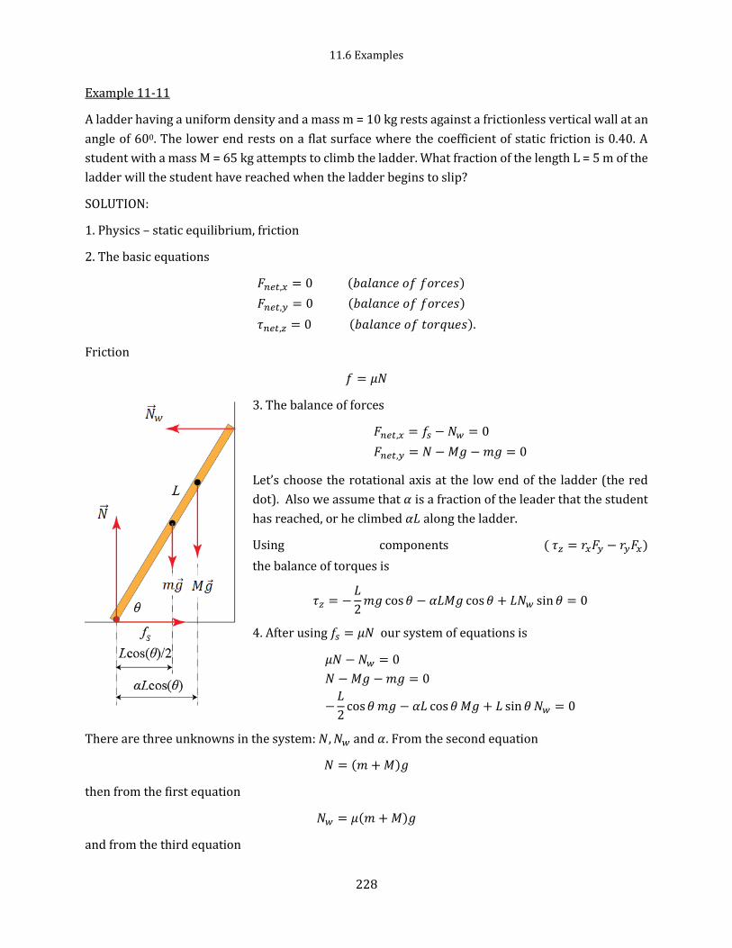
11.6 Examples
228
Example 11-11
A ladder having a uniform density and a mass m = 10 kg rests against a frictionless vertical wall at an
angle of 600. The lower end rests on a flat surface where the coefficient of static friction is 0.40. A
student with a mass M = 65 kg attempts to climb the ladder. What fraction of the length L = 5 m of the
ladder will the student have reached when the ladder begins to slip?
SOLUTION:
1. Physics – static equilibrium, friction
2. The basic equations
𝐹𝑛𝑒𝑡,𝑥 = 0 (𝑏𝑎𝑙𝑎𝑛𝑐𝑒 𝑜𝑓 𝑓𝑜𝑟𝑐𝑒𝑠)
𝐹𝑛𝑒𝑡,𝑦 = 0 (𝑏𝑎𝑙𝑎𝑛𝑐𝑒 𝑜𝑓 𝑓𝑜𝑟𝑐𝑒𝑠)
𝜏𝑛𝑒𝑡,𝑧 = 0 (𝑏𝑎𝑙𝑎𝑛𝑐𝑒 𝑜𝑓 𝑡𝑜𝑟𝑞𝑢𝑒𝑠).
Friction
𝑓 = 𝜇𝑁
3. The balance of forces
𝐹𝑛𝑒𝑡,𝑥 = 𝑓𝑠 − 𝑁𝑤 = 0
𝐹𝑛𝑒𝑡,𝑦 = 𝑁 − 𝑀𝑔 − 𝑚𝑔 = 0
Let’s choose the rotational axis at the low end of the ladder (the red
dot). Also we assume that 𝛼 is a fraction of the leader that the student
has reached, or he climbed 𝛼𝐿 along the ladder.
Using components ( 𝜏𝑧 = 𝑟𝑥𝐹𝑦 − 𝑟𝑦𝐹𝑥)
the balance of torques is
𝜏𝑧 = −𝐿
2𝑚𝑔 cos 𝜃 − 𝛼𝐿𝑀𝑔 cos 𝜃 + 𝐿𝑁𝑤 sin 𝜃 = 0
4. After using 𝑓𝑠 = 𝜇𝑁 our system of equations is
𝜇𝑁 − 𝑁𝑤 = 0
𝑁 − 𝑀𝑔 − 𝑚𝑔 = 0
−𝐿
2cos 𝜃 𝑚𝑔 − 𝛼𝐿 cos 𝜃 𝑀𝑔 + 𝐿 sin 𝜃 𝑁𝑤 = 0
There are three unknowns in the system: 𝑁, 𝑁𝑤 and 𝛼. From the second equation
𝑁 = (𝑚 + 𝑀)𝑔
then from the first equation
𝑁𝑤 = 𝜇(𝑚 + 𝑀)𝑔
and from the third equation

11. Equilibrium
229
𝛼 =𝐿 sin 𝜃 𝑁𝑤 − −
𝐿2
cos 𝜃 𝑚𝑔
𝐿 cos 𝜃 𝑀𝑔=
𝐿 sin 𝜃 𝜇(𝑚 + 𝑀)𝑔 − −𝐿2
cos 𝜃 𝑚𝑔
𝐿 cos 𝜃 𝑀𝑔
and after some algebra
𝛼 = 𝜇 (𝑚 + 𝑀
𝑀) tan 𝜃 −
1
2(
𝑚
𝑀)
5. Calculations
𝛼 = 0.4 (10 𝑘𝑔 + 65 𝑘𝑔
65 𝑘𝑔) tan 600 −
1
2(
10 𝑘𝑔
65 𝑘𝑔) = 0.72
or the student will beat ℎ = 0.72 ∙ 5 𝑚 ∙ sin 600 = 3.1 𝑚 above the ground.
6. Looking back.
Units (actually no units) are correct.
I cannot imagine some special case with an obvious solution.
The ladder problem is a classic example in most textbooks. You might noticed that we took into account
only one frictional force, namely from the floor. Most discussions of this problem assume that the static
frictional force between the ladder and wall can be ignored. Can it? Indeed, we would expect one.
However in this case the problem is getting very complicated with no unique solution (four unknowns
but three equations!). Without modeling the elasticity of the ladder, it is not possible to solve the ladder
problem for all the external forces. It is interesting how a simple problem can get complicated in no time,
just by adding one more force
More for the ladder problem: We can analyze the major dependences.
a) let’s see how 𝛼 changes with 𝑀 for fixed 𝜃 = 600, 𝑚 = 10 𝑘𝑔 and 𝜇 = 0.4
This is quite interesting. As the mass
increases the fraction decreases but
only to a certain critical point on the
ladder.

11.6 Examples
230
b) let’s explore the angle dependence for 𝑀 = 65 𝑘𝑔
As the angle increase, the safe point on
the ladder goes up in a non-linear way.
For given conditions, At about 700 it is
safe to stand at the top of the ladder.

12. The Law of Gravitation
231
12 The Law of Gravitation
This law has been called “the greatest generalization achieved by the human mind”. For centuries
scientists and curious minds tried to understand the motions of planets among the stars, and causes
behind the motion. Ancient Greeks deduced from simple observations that planets went around the
sun. However, they were not able to identify exactly how the planets went around the sun, with
exactly what causes. By the beginning of the fifteenth century there were heated debates as to
whether the planets really went around the sun or not. These debates were mostly philosophical. It
was Tycho Brahe, a Danish astronomer, who suggested to resolve the dispute by accurate
measurements of positions of the planets. After a couple decades of careful observations he published
extensive tables of data. Years later a mathematician Johannes Kepler derived three laws of planetary
motion based on Brahe’s tables of data. 1) All planets move in elliptical orbits with the Sun at one
focal point, 2) the radius vector drawn from the Sun to a planet sweeps out equal areas in equal time
intervals, and 3) the square of the orbital period of any planet is proportional to the cube of the semi-
major axis of the elliptical orbit. However still no explanation was provided for causes of motion.
Decades later, in 1686, Isaac Newton published his law of gravitation
12.1 Newton’s law of gravitation
The Law of Gravitation is that two bodies attract each other with a force upon each other which varies
inversely as the square of the distance between them, and varies directly as the product of their
masses. Mathematically we can write that great law as a simple formula

12.1 Newton’s law of gravitation
232
𝐹 = 𝐺 𝑚1𝑚2
𝑟2, (12.1)
where 𝑚1 and 𝑚2 are masses of bodies, 𝑟 is the distance between them, and 𝐺 is a fundamental
proportionality constant called the universal gravitational constant or simply gravitational constant.
In SI unites its value is
𝐺 = 6.67408 × 10⁻¹¹ 𝑁 ⋅ 𝑚2 𝑘𝑔2⁄
Please note that this is a recommended value by International Council for Science: Committee on Data
for Science and Technology (CODATA) as of 2014. Most standard textbooks, as well as Wikipedia, use
𝐺 = 6.67384 × 10⁻¹¹𝑁 ⋅ 𝑚2 𝑘𝑔2⁄ that is a value based on less precise measurements. It is also
interesting to note that it took 112 years, after publishing the law of gravitation by Newton, to
measure 𝐺 for the first time.
We can also write the law in a vector form (remember that forces are vectors)
�⃗�21 = 𝐺𝑚1𝑚2
𝑟212 �̂�21 (12.2)
where �̂�21 is a unit vector in the direction from 1 toward 2 (note that 𝑟21 = 𝑟2 − 𝑟1).
Figure 12.1 Notations for positions and forces
Using the components we can write
𝐹21,𝑥 = 𝐺𝑚1𝑚2
𝑟213
(𝑥2 − 𝑥1), 𝐹21,𝑦 = 𝐺𝑚1𝑚2
𝑟213
(𝑦2 − 𝑦1), 𝐹21,𝑧 = 𝐺𝑚1𝑚2
𝑟213
(𝑧2 − 𝑧1).
In case of three or more objects we simply use the superposition of forces to find a net force on every
object in a system. For example, a net force on object 1 from n other objects is written as
�⃗�𝑖1 = ∑ 𝐺𝑚1𝑚𝑖
𝑟𝑖12 �̂�𝑖1
𝑛
𝑖=2
Having the law of gravitation together with second newton’s law we have everything required to
derive many consequences of these two principles. The problem of motion of objects interacting by
the law of gravity can analytically be solved only for two objects. For three or more objects the
problem can be treated only numerically.
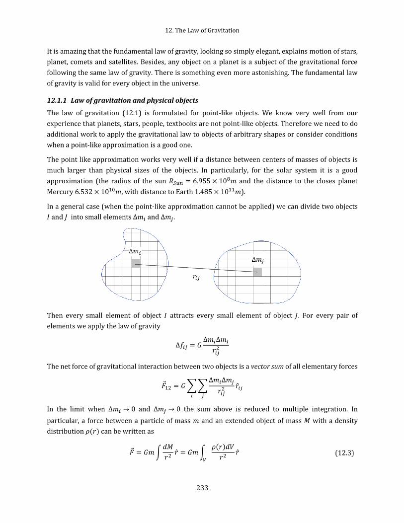
12. The Law of Gravitation
233
It is amazing that the fundamental law of gravity, looking so simply elegant, explains motion of stars,
planet, comets and satellites. Besides, any object on a planet is a subject of the gravitational force
following the same law of gravity. There is something even more astonishing. The fundamental law
of gravity is valid for every object in the universe.
12.1.1 Law of gravitation and physical objects
The law of gravitation (12.1) is formulated for point-like objects. We know very well from our
experience that planets, stars, people, textbooks are not point-like objects. Therefore we need to do
additional work to apply the gravitational law to objects of arbitrary shapes or consider conditions
when a point-like approximation is a good one.
The point like approximation works very well if a distance between centers of masses of objects is
much larger than physical sizes of the objects. In particularly, for the solar system it is a good
approximation (the radius of the sun 𝑅𝑆𝑢𝑛 = 6.955 × 10⁸𝑚 and the distance to the closes planet
Mercury 6.532 × 10¹⁰𝑚, with distance to Earth 1.485 × 10¹¹𝑚).
In a general case (when the point-like approximation cannot be applied) we can divide two objects
𝐼 and 𝐽 into small elements Δ𝑚𝑖 and Δ𝑚𝑗.
Then every small element of object 𝐼 attracts every small element of object 𝐽. For every pair of
elements we apply the law of gravity
Δ𝑓𝑖𝑗 = 𝐺Δ𝑚𝑖Δ𝑚𝐼
𝑟𝑖𝑗2
The net force of gravitational interaction between two objects is a vector sum of all elementary forces
�⃗�12 = 𝐺 ∑ ∑Δ𝑚𝑖Δ𝑚𝑗
𝑟𝑖𝑗2 �̂�𝑖𝑗
𝑗𝑖
In the limit when Δ𝑚𝑖 → 0 and Δ𝑚𝑗 → 0 the sum above is reduced to multiple integration. In
particular, a force between a particle of mass 𝑚 and an extended object of mass 𝑀 with a density
distribution 𝜌(𝑟) can be written as
�⃗� = 𝐺𝑚 ∫𝑑𝑀
𝑟2�̂� = 𝐺𝑚 ∫
𝜌(𝑟)𝑑𝑉
𝑟2𝑉
�̂� (12.3)

12.1 Newton’s law of gravitation
234
where the integration is carried out over the volume of an object.
Let us consider a simple application, namely a force of gravity between a homogeneous bar of length
𝐿 and mass 𝑀 and a particle of mass 𝑚 located at distance 𝑎 from the bar.
Keeping in mind that 𝑑𝑀 can be written as 𝑑𝑀 = (𝑀 𝐿⁄ )𝑑𝑥 = 𝜆𝑑𝑥, where 𝜆 is a linear density, we can
write the total gravitational force exerted by the bar on the particle as
�⃗� = 𝐺𝑚 ∫𝑑𝑀
𝑥2
𝑎+𝐿
𝑎
𝑖̂ = 𝐺𝑚 ∫𝜆𝑑𝑥
𝑥2
𝑎+𝐿
𝑎
𝑖̂ = 𝐺𝑚 ∫ (𝑀
𝐿)
𝑑𝑥
𝑥2
𝑎+𝐿
𝑎
𝑖̂ =
𝐺𝑚𝑀
𝐿𝑖̂ ∫
𝑑𝑥
𝑥2
𝑎+𝐿
𝑎
=𝐺𝑚𝑀
𝐿𝑖̂(−1) (
1
𝑎 + 𝐿−
1
𝑎)
and finally
�⃗� =𝐺𝑚𝑀
𝐿
𝐿
𝑎(𝑎 + 𝐿)𝑖̂ = 𝐺
𝑚𝑀
𝑎(𝑎 + 𝐿)𝑖 ̂
We can see that in the limit 𝐿 → 0,
�⃗� = lim𝐿→0
𝐺𝑚𝑀
𝑎(𝑎 + 𝐿)𝑖̂ = 𝐺
𝑚𝑀
𝑎2𝑖̂
and the force of gravity corresponds to a force between two point-like masses. Additionally, if 𝑎 ≫ 𝐿
(the distance between the objects is much larger that objects), then again we have it like a force
between two particles.
Generally, calculations of multiple integrals, in cases of physical objects of various shapes, can be quite
cumbersome. However, for this chapter we only need a couple special cases, namely gravitational
force between a star and a planet, between a planet and a satellite, and between a planet and an object
on or close to a planet’s surface.
12.1.2 Newton's shell theorem
Most planets and starts are spheres (or almost spheres) with spherically symmetric mass distributions.
Then we can use Newton’s shell theorem that states “A uniform spherical shell of matter attracts a
particle that is outside the shell if all the shell’s mass were concentrated at its center”. From the shell
theorem follows that bodies having a spherically symmetric mass distribution over their volume

12. The Law of Gravitation
235
interact as if their masses were concentrated at the centers of these spheres
𝐹 = 𝐺 𝑚1𝑚2
𝑅2 (12.4)
Planets and stars are either far away from each other (𝑅 ≫ 𝑟1, 𝑟2) or have geometric shapes very close
to spherical. Therefore equation (12.4) is a very good one for celestial mechanics.
For a physical object outside a uniform solid sphere or spherical shell
the magnitude of gravitational force on this object is
𝐹 = 𝐺 𝑚𝑀
(𝑅 + ℎ)2 (12.5)
where 𝑅 is the radius of a sphere and ℎ is the distance to the sphere’s surface from a physics object. If
a size of a physics object is much less than 𝑅 + ℎ then the physics object can be treated as a point like
object (its real shape does not matter). Equation (12.5) is a very good approximation for gravitational
for between a planet and a satellite and for any objects on or above a surface of a planet.
Near the Earth surface ℎ ≪ 𝑅 then
1
(𝑅 + ℎ)2=
1
𝑅2
1
(1 + ℎ 𝑅⁄ )2≈
1
𝑅2(1 − 2
ℎ
𝑅+ ⋯ ),
where we have neglected the quadratic and higher-order terms in (h/R)2 since h/R is very small. For
example, at the top of Everest we have ℎ/𝑅 ≈ 1.4 × 10⁻³. In most cases, there is no need to take into
account insignificant variations in the force of gravity. Within the accuracy 10−3, we can consider that
for objects on Earth the force of gravity is constant and independent of the altitude.
It is instructive to evaluate magnitudes of gravitational force between some objects. Thus the force
between Earth and Sun is 3.53 × 10²²𝑁 (quite a large number!), the force between a human body and
Earth is simply its weight, for a 60 kg body it is about 590 𝑁, the force between two humans (assume

12.2 Acceleration due to gravity g
236
they have spherical shapes) separates by a distance of 10 meters is 2.4 × 10⁻⁹𝑁 (or about 10,000
times less than a weight of mosquito). As we can see gravitational force between objects on Earth is
very small comparing to their weights.
Some people believe that positions of stars at birth influence somebody’s life. Assume that they are
taking about gravitational force. Let’s calculate gravitational force from the closest star outside the
solar system (Sirius) on a human body at birth, we can easily get it is about 1.6 × 10⁻⁷𝑁, or about ten
times less than one eyelash hair. (### check these numbers)
12.1.3 Gravitational and Inertial Masses
Expressing the law of gravity (12.1) we silently assumed that masses in the law are the same masses
that we have in the second newton’s law (4.5). However this assumption is not solid without
additional insight. The law of gravity and the second newton’s law are two independent laws. In the
second newton’s law mass characterizes the property of inertia of motion, or inertial mass is the
property of an object that measures the object’s resistance to acceleration. In the law of gravity mass
characterizes a property of objects to attract each other with gravitational force. Therefore it is
reasonable to ask a question if we should rather assign 𝑚𝐼 for the inertial mass, and 𝑚𝐺 for the
gravitational mass and to treat them differently. It is clear that only experiments can answer this
questions. From the second Newton’s law follows for the free-fall acceleration
𝑔 =𝐹𝑔
𝑚𝐼= 𝐺
𝑀𝐸
𝑅𝐸2
𝑚𝐺
𝑚𝐼
where 𝑀𝐸 is the mass of Earth, and 𝑅𝐸 is the radius of Earth. Experiments show that free fall
acceleration 𝑔 is the same for all objects at the same location. Since 𝐺, 𝑀𝐸 , 𝑅𝐸 are constants for the
same locations, then the ratio 𝑚𝐺 𝑚𝐼⁄ must be the same for all objects. At this time highly precise
measurement show no difference between the two masses with accuracy 10−18. The equivalence of
inertial and gravitational masses (the equivalence principle)
𝑚𝐼 = 𝑚𝐺
is at the foundation of general theory of relativity.
12.2 Acceleration due to gravity g
In previous chapters we use for the magnitude of the gravitational force on objects from Earth as
𝐹 = 𝑚𝑔
Assuming that the earth is a uniform sphere of radius 𝑅𝐸 and mass 𝑀𝐸 , then a small body of mass 𝑚
at the earth’s surface (a distance 𝑅𝐸 from its center) experiences gravitational force
𝐹 = 𝐺𝑚𝑀𝐸
𝑅𝐸2 = 𝑚𝑔
We can easily find that the acceleration due to gravity at the earth’s surface

12. The Law of Gravitation
237
𝑔 = 𝑔𝐸 = 𝐺𝑀𝐸
𝑅𝐸2 (12.6)
The acceleration due to gravity 𝑔 is independent of the mass 𝑚 of the object. By the way, equation
(12.6) provided a way to calculate the mass of the Earth since the radius was known since ancient
times.
However we need to note that under closer examination the free-fall acceleration 𝑔 is not a constant.
In reality it is a bit different from (12.6) for three reasons.
First, Earth is not uniform. Its density varies radially, and the density of the crust varies slightly from
region to region (larger in mountain regions).
Second, Earth is not a perfect sphere but approximately an ellipsoid flattered at the poles and bulging
at the equator. Its polar radius is smaller than its equatorial radius by about 21 km (that is 0.33%
difference). So, a point at the poles is closer to the dense core of Earth, than a point on the equator,
and the free-fall acceleration is large at the poles.
Third, Earth is rotating. Therefore a point on equator has the largest centripetal force due do the
rotation. We can easily analyze this effect using our knowledge from previous chapters. Let us
consider an object located on the equator.
There are two forces acting on the object, namely the gravitational force and a normal force. We
normally assume that the magnitude of the normal force is 𝑁 = 𝑚𝑔. From (12.6)
𝑔𝐸 = 𝐺𝑀𝐸
𝑅𝐸2
Then we can write
𝑁 − 𝑚𝑔𝐸 = −𝑚𝑣2
𝑅, 𝑚𝑔 − 𝑚𝑔𝐸 = −
𝑚𝑣2
𝑅
then
𝑔 = 𝑔𝐸 −𝑣2
𝑅= 𝑔𝐸 − 𝜔2𝑅
where 𝜔 is the angular speed of Earth. Practically the equation above says that free-fall acceleration
is gravitational acceleration minus centripetal acceleration. For an object on the equator this

12.3 Gravitational potential energy
238
centripetal acceleration is very small (about 0.034 m/s2 compared with 9.8 m/s2). If the Earth had a
perfectly spherical shape, then an object moved from a pole to the equator would “lose” 0.35% of its
weight. Accounting for the deviation from the ideal spherical shape of Earth makes such “loss of
weight” even larger, namely about 0.5%. Therefore the free fall acceleration changes with latitude
from 9.780 m/s2 at the equator to 9.832 m/s2 at the poles. For this course neglecting the difference
between 𝑔 and 𝑔𝐸 is often well justified. Therefore within the accuracy 10−2 we can consider the free-
fall acceleration as constant and independent of the altitude and position on Earth. The standard
acceleration of gravity recommended by CODATA is
𝑔 = 9.80665 𝑚 𝑠2⁄
* This acceleration corresponds to a location at 45 degrees of latitude. For practical purposes in this
book we use 𝑔 = 9.8 𝑚 𝑠2⁄ .
12.3 Gravitational potential energy
In chapter 7 we introduced potential energy for conservative forces, which is which is energy
associated with a configuration of objects. The gravitational force (12.1) is a conservative force (no
proof here). We already evaluated gravitational potential energy as 𝑈 = 𝑚𝑔(𝑦𝑓 − 𝑦𝑖). However that
evaluation has been done under assumption for the free-fall acceleration to be constant. This
assumption is a good one as soon as objects are not too far from Earth’s surface comparing to Earth’s
radius. Now we want to derive a more general expression for the gravitational potential energy. A
conservative force and potential energy are connected (7.2)
𝑈(𝑟) = − ∫ 𝐹(𝑟′)𝑑𝑟′𝑟
𝑟0
We can easily notice that the gravitational force (12.1) on object 𝑚 is spherically symmetrical
�⃗� = −𝐺𝑚𝑀
𝑟2�̂�
where 𝑟 is a vector directed from the origin to the body (that is why we have the negative sign here).
Since the integral above is independent of paths we can integrate the force along a radius
𝑈(𝑟) = − ∫ 𝐹(𝑟′)𝑑𝑟′𝑟
𝑟0
= 𝐺𝑚𝑀 ∫𝑑𝑟′
𝑟′2
𝑟
𝑟0
= −𝐺𝑚𝑀 (1
𝑟−
1
𝑟0)
For any potential energy the choice of a reference point is entirely arbitrary. It is common to choose
it where the force is zero. Thus setting 𝑈(𝑟) = 0 at 𝑟 = ∞ where 𝐹(𝑟) → 0 we get
𝑈(𝑟) = −𝐺𝑚𝑀
𝑟 (12.7)
The equation above can be applied to any two particles with masses 𝑚 and 𝑀. The gravitational
potential energy between two objects increases with distance because the gravitational force attracts
masses.

12. The Law of Gravitation
239
The gravitational potential energy for a system with more than two particles is the sum over all pairs
of particles. For example, for three particles we have
𝑈𝑡𝑜𝑡𝑎𝑙 = −𝐺 (𝑚1𝑚2
𝑟12+
𝑚1𝑚3
𝑟13+
𝑚2𝑚3
𝑟23)
The absolute value of the gravitational potential characterizes the work needed to separate the
particles by an infinite distance.
By inspecting formula (12.7) one may be wondering why do we have two definitions for the
gravitational potential energy, namely 𝑈 = 𝑚𝑔ℎ and (12.7). Let us consider a change in the
gravitational potential energy of an object raised from the ground of Earth to a height ℎ
𝑈(𝑅𝐸 + ℎ) − 𝑈(𝑅𝐸) = −𝐺𝑚𝑀𝐸
𝑅𝐸 + ℎ+ 𝐺
𝑚𝑀𝐸
𝑅𝐸= 𝐺𝑚𝑀𝐸 (
1
𝑅𝐸−
1
𝑅𝐸 + ℎ) = 𝐺𝑚𝑀𝐸
ℎ
𝑅𝐸(𝑅𝐸 + ℎ)
When the height ℎ is very small compared with the radius of Earth 𝑅𝐸 , we can disregard terms ℎ 𝑅⁄ ,
yielding
𝑈(𝑅𝐸 + ℎ) − 𝑈(𝑅𝐸) ≈ 𝐺𝑚𝑀𝐸
ℎ
𝑅𝐸2 = 𝑚ℎ
𝐺𝑀𝐸
𝑅𝐸2 = 𝑚ℎ𝑔
since according to (12.6) the last term 𝐺𝑀𝐸 𝑅𝐸2⁄ in the equation is free fall acceleration 𝑔.
12.4 Motion of planets and satellites
Motion of three or more objects interacting by force of gravity has been a challenging problem for
both physicists and mathematicians since Newton. It has been demonstrated that even 3-body
problem does not have an analytic solution. There are either infinite series solutions or solutions for
specific modes of motion. Interesting enough French mathematician and physicist Poincaré working
with the problem laid the foundations of modern chaos theory (the butterfly effect). Thus, motion of
celestial (or astronomical) objects can only be calculated numerically8. Quite often when we do not
need high accuracy we can substitute a many-body problem with a two-body one. If one of the bodies
has a mass much larger than the other, then we practically dealing with a one-body problem moving
in a gravitational field of a heavy body. If we disregard interaction between the planets in the solar
system (a simplified view of the solar system) comparing to their interaction with the Sun, then we
approximate their motion as one-body motion around the sun. Using astronomical data you can easily
evaluate quality of this approximation by comparing gravitational forces in the solar system.
For the Earth-Sun system we have that the mass of the Sun (2 × 1030𝑘𝑔) is 332,000 times the mass
of the Earth (6 × 1024𝑘𝑔). Hence the Sun can be considered to be stationary to a high degree of
accuracy, and the Earth can be expected to be revolving around a fixed center. Besides, the Sun and
8 Millennium Simulation or Millennium Run is likely the most impressive N-body simulation. The Millennium Run was populated by about 20 million "galaxies" to trace the evolution of the matter distribution in a cubic region of the Universe over 13 billion light-years.

12.4 Motion of planets and satellites
240
the Earth have almost spherical shapes, and also the distance between the Sun and the Earth is much
larger than diameters of the Sun and the Earth. Therefore, we can treat them as point-like objects. The
other example is motion of satellites orbiting the Earth. Sure, their gravitational interactions is many
orders of magnitude less than the force of gravity from the planet.
Equation of motion for an object of mass 𝑚 (a planet or a satellite) in a field of a heavy object of mass
𝑀 (a star or a planet accordingly) can be written in the form
𝑚𝑑�⃗�
𝑑𝑡= −𝐺
𝑚𝑀
𝑟2�̂� (12.8)
where 𝑟 is the radius vector of the planet relative to the mass 𝑀. This is a second-order ordinary
differential equation. Solving it together with initial conditions provide a position of the planet as a
function of time. All Kepler’s laws can be derived from such solutions. Such an exercise is a good one
for courses of classical mechanics and mathematical physics.
Here are the most important result from analysis of (12.8). The force of gravity acting on a point mass
is directed along the radius vector. The moment of this force about the center of force is zero, and for
angular momentum 𝐿 (10.9) we have
𝑑𝐿
𝑑𝑡= 𝑟 × �⃗� = 𝑟 ×
𝑑
𝑑𝑡𝑚�⃗� = 0
Therefore the angular momentum of a point mass in our case has a constant magnitude as well as
direction
𝐿 = 𝑟 × 𝑚�⃗� = 𝑐𝑜𝑛𝑠𝑡.
For an elementary displacement this equation can be rewritten as
𝐿 = 𝑚𝑟 × �⃗� = 𝑚𝑟 ×𝑑𝑟
𝑑𝑡
Hence the elementary displacement 𝑑𝑟 and the radius vector 𝑟 are in a plane perpendicular to the
angular momentum �⃗⃗�. This means that all the time the motion happens in the same plane.
In polar coordinates (𝑟, 𝜑) the general solution (Kepler orbit) is given by
𝑟(𝜑) =𝑐
1 + 𝜖 cos 𝜑
where 𝑐 is a constant and 𝜖 is the eccentricity. There are four different Kepler orbits (depending on
initial conditions). For total energy 𝐸 < 0 the solutions are bounded orbits either a circle (𝜖 = 0) or
an ellipse (0 < 𝜖 < 1). For total energy 𝐸 ≥ 0 the solution are either a parabola (𝐸 = 0, 𝜖 = 0) or a
hyperbola (𝐸 > 0, 𝜖 > 1).
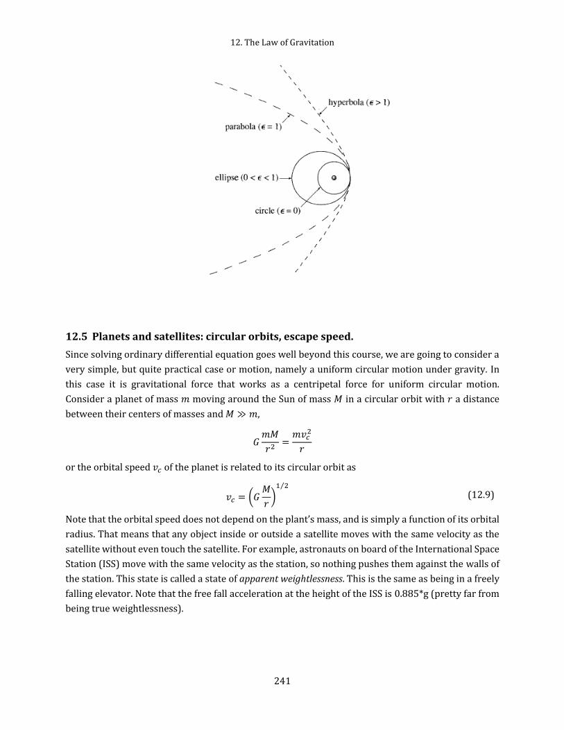
12. The Law of Gravitation
241
12.5 Planets and satellites: circular orbits, escape speed.
Since solving ordinary differential equation goes well beyond this course, we are going to consider a
very simple, but quite practical case or motion, namely a uniform circular motion under gravity. In
this case it is gravitational force that works as a centripetal force for uniform circular motion.
Consider a planet of mass 𝑚 moving around the Sun of mass 𝑀 in a circular orbit with 𝑟 a distance
between their centers of masses and 𝑀 ≫ 𝑚,
𝐺𝑚𝑀
𝑟2=
𝑚𝑣𝑐2
𝑟
or the orbital speed 𝑣𝑐 of the planet is related to its circular orbit as
𝑣𝑐 = (𝐺𝑀
𝑟)
1 2⁄
(12.9)
Note that the orbital speed does not depend on the plant’s mass, and is simply a function of its orbital
radius. That means that any object inside or outside a satellite moves with the same velocity as the
satellite without even touch the satellite. For example, astronauts on board of the International Space
Station (ISS) move with the same velocity as the station, so nothing pushes them against the walls of
the station. This state is called a state of apparent weightlessness. This is the same as being in a freely
falling elevator. Note that the free fall acceleration at the height of the ISS is 0.885*g (pretty far from
being true weightlessness).

12.5 Planets and satellites: circular orbits, escape speed.
242
Since the period of revolution is circumference divided by speed, then
𝑇𝑐 =2𝜋𝑟
𝑣
Substituting the orbital speed from (12.9) the preceding expression becomes
𝑇𝑐 =2𝜋𝑟3 2⁄
(𝐺𝑀)1 2⁄ (12.10)
We can also apply equation (12.10) to satellite motion around a planet if we consider 𝑀 as mass of a
planet, and 𝑚 as mass of a satellite.
Quite often for satellite motion it is convenient to denote the distance between the centers of masses
𝑟 as 𝑟 = 𝑅 + ℎ where 𝑅 is the radius of the planet, and ℎ is a distance form surface of the planet to a
satellite, then
𝑣𝑐 = (𝐺𝑀
𝑅 + ℎ)
1 2⁄
𝑇𝑐 =2𝜋(𝑅 + ℎ)3 2⁄
(𝐺𝑀)1 2⁄ (12.11)
Using (12.11) we can calculate the orbital speed and the period for the International Space Station
with ℎ = 250 miles or about 400 𝑘𝑚 that gives us 𝑣𝑐 = 7670 𝑚/𝑠 and 𝑇𝑐 = 92 minutes. For the Earth
orbiting the Sun we get for the orbital velocity 𝑣𝑐 = 30 𝑘𝑚/𝑠 (or about 70,000 mph), the period (a
year) is 365.3 days.
Some communication satellites are moving in a circle in the earth’s equatorial plane. They are at such
height that they always remain above the same point. Such orbits are called as geosynchronous orbits.
Using 24 hours for the period of revolution we can find from (12.11)
ℎ + 𝑅 = (𝑇𝑐
2𝐺𝑀
4𝜋2 )
1 3 ⁄
that such satellites must be placed at about ℎ=35,800 km above the Earth surface.

12. The Law of Gravitation
243
Since we assumed that 𝑀 ≫ 𝑚 (the heavier object is located at the origin and does not move) then
then the total mechanical energy 𝐸 of the two-body system is
𝐸 =1
2𝑚𝑣2 − 𝐺
𝑚𝑀
𝑟
Using (12.9) for a circular orbit gives
𝐸 =1
2𝐺
𝑚𝑀
𝑟− 𝐺
𝑚𝑀
𝑟= −𝐺
𝑚𝑀
2𝑟
One can see that for circular orbits the kinetic energy is equal to one-half the absolute value of the
potential energy. The absolute value of total energy 𝐸 is binding energy of the system. It is this amount
of energy is needed for the system to separate the two masses infinitely. Thus we can derive another
characteristic speed, also called escape speed. This is the minimum value of the initial speed needed
to let the object of mass 𝑚 to escape the gravitational force of object with mass 𝑀 (for example for a
satellite to leave the Earth without coming back). Let at the surface of the Earth the initial speed is 𝑣𝑖
and 𝑟 = 𝑅𝐸 . When the satellite approaches 𝑟 → ∞ its speed 𝑣𝑓 → 0, thus 𝐾𝑓 → 0 anf 𝑈𝑓 → 0 Using
conservation of energy gives
1
2𝑚𝑣𝑖
2 − 𝐺𝑚𝑀𝐸
𝑅𝐸= 0
and we obtain
𝑣𝑖 = 𝑣𝑒𝑠𝑐 = (2𝐺𝑀
𝑅𝐸)
1 2⁄
(12.12)
Note that the escape speed is independent of the mass of the object, and independent of the direction
of the velocity (but sure ignores air resistance). Equation (12.12) can be applied to any object
launched from any planet.
*** add following topics
How to change an orbit of a satellite
Black holes and escape speed
Tides: Moon-Earth interaction
Shell theorem – gravity inside a planet
Calculating gravitational force from a physical object – much easier to calculate the potential,
then force
Dark matter

12.6 Examples
244
12.6 Examples
Example 12-1
A satellite with a mass of 1000 kg is placed in Earth orbit at an orbit of 500 km above the surface.
Assuming a circular orbit,
a) How long does the satellite take to complete one orbit?
b) What is the satellite’s orbital speed?
c) What is the minimum energy necessary to place this satellite in orbit (assume there is no air
resistance)?
d) For how many miles would this energy power an automobile? (Assume 1 gal. of gasoline
produces 1.1*108 J of energy, and this energy is sufficient to operate a car for 25 miles)
Example 12-2
Two spherical objects of masses 𝑚1and 𝑚2 are released from rest at a separation distance of 𝐿. Find
their speeds and positions when their separation distance is 𝑟. Assume that the first particle initially
is at the origin.
Example 12-3
The fastest possible rate of rotation of a planet is that for which the gravitational force on material at
the equator just barely provides the centripetal force needed for the rotation. Calculate this rotation
period for Earth.
Example 12-4
The Schwarzschild radius is a distance from a black hole where the escape velocity equals the speed
of light (even light cannot escape from a black hole). Determine the Schwarzschild radius for a black
hole with the mass of the Sun.
Example 12-5
Consider an asteroid of a size of Texas (see Armageddon movie). Assume that the asteroid has a
spherical shape, its radius is 400 𝑘𝑚 and density is 5.5 𝑔 𝑐𝑚3⁄ . Estimate speed needed to provide to
a baseball to make it a satellite orbiting the asteroid just above the surface.
Example 12-6
Calculate the time taken by the Earth to fall from the orbit onto the Sun if its instantaneous radial
velocity became zero.
13. Periodic Motion
245
13 Periodic Motion
We encounter periodic motion in both our everyday lives and in science and engineering. Periodic
motion is also a basis for any time keeping device, from the Earth rotation (24 hours) to atomic clocks.
We also use vibration, oscillation, or harmonic motion as synonyms for periodic motion.
In this chapter we are going to study periodic motion caused by a force that we know explicitly. Thus
we can understand all the details from first principles.
13.1 Simple harmonic motion
There are remarkable equations in physics which appear in various branches of physics, so that vary
many effects can be described by same equations. Very many of such equations are linear differential
equations with constant coefficients. Examples of phenomena described by such equations are the
oscillations of a mass on a spring; the oscillations of current in an electrical circuit.
The simplest mechanical system whose motion follows a linear differential equation with constant
coefficients is a mass on a spring. Such a system is also called a harmonic oscillator. Consider a block
of mass 𝑚 attached to the end of a horizontal spring. The block is free to move on a frictionless surface.
In this case we have only one force affecting the motion, namely the spring force.
�⃗� = −𝑘�⃗�
The minus sign tell us that the spring force is a restoring force pulling always back in the direction of
the equilibrium and opposite to the displacement.

13.1 Simple harmonic motion
246
Thus the second Newton’s law, mass times the acceleration, must equal to – 𝑘𝑥
𝑚𝑑2𝑥
𝑑𝑡2= −𝑘𝑥 (13.1)
There is a more common form for this equation, namely
𝑑2𝑥
𝑑𝑡2= −𝜔2𝑥 (13.2)
where, in case of the spring force
𝜔 = (𝑘
𝑚)
12⁄
(13.3)
Equation (13.2) is called a simple harmonic motion equation (SHM), and it plays an extraordinary
role in practically all fields of physics. There are two major reasons for this equation to be the
exceptional one. First, harmonic motion is caused by a force that is linear proportional to the
displacement. For small displacements any force can be expanded into a Taylor series, where the first
linear term, is a leading one. Therefore, physics of a simple harmonic motion is often the first step in
studying many periodic motions. Second, many oscillating systems “resonate” to external harmonic
oscillations when their frequencies of oscillations are close.
Mathematically, the SHM differential equation has a very simple general solution as
𝑥(𝑡) = 𝐶1 cos 𝜔𝑡 + 𝐶2 sin 𝜔𝑡 (13.4)
or in the equivalent form
𝑥(𝑡) = 𝐴 cos(𝜔𝑡 + 𝜑) (13.5)
it is easy to test these solutions by a simple substitution of (13.5) into (13.2).
Let us first analyze the meanings of all terms in the solution (13.5). The constant 𝜔 is called the
angular frequency of the motion (units - radians per second). It is the number of radians by which the
phase changes in a second. That is determined by the differential equation. We know that the
trigonometric function cos 𝑥 is periodic and repeats itself every time 𝜔𝑡 increases by 2𝜋. Then
𝜔𝑡 + 2𝜋 = 𝜔(𝑡 + 𝑇)
where 𝑇 is the period of the motion, and hence

13. Periodic Motion
247
𝑇 =2𝜋
𝜔 (13.6)
And for a spring it becomes
𝑇 = 2𝜋√𝑚
𝑘 (13.7)
It is very common to also use frequency 𝑓 of the motion. The frequency represents the number of
oscillations that the particle makes per unit time
𝑓 =1
𝑇=
𝜔
2𝜋 (13.8)
The units for the frequency are cycles per second (s-1) or hertz (Hz). For the angular frequency:
𝜔 = 2𝜋𝑓 =2𝜋
𝑇 (13.9)
The other constants of motion (𝐴 and 𝜑) are not determined by the equation, but by how the motion
is started. For a second order differential equations we need two initial conditions to define a specific
solution. Very often it is done by setting an initial position and velocity at some initial time, i.e.
𝑥(𝑡 = 0) = 𝑥0, 𝑣(𝑡 = 0) = 𝑣0. Of these constants, 𝐴 measures the maximum displacement attained
by the mass, and is called the amplitude of oscillation. We can see that by plotting a graph for two
values of 𝐴 namely 𝐴 and 2𝐴.
The constant 𝜑 is sometimes called the phase of the oscillation. But that is a confusion, because other
people call 𝜔𝑡 + 𝜑 as the phase, and say the phase changes with time. We might say that 𝜑 is a phase
shift from some defined zero. The following graph should help in visualizing this

13.1 Simple harmonic motion
248
We can obtain the linear velocity of a particle undergoing simple harmonic motion by differentiating
(13.5) with respect to time
𝑣(𝑡) =𝑑𝑥
𝑑𝑡= −𝐴𝜔 sin(𝜔𝑡 + 𝜑) (13.10)
And the acceleration is
𝑎(𝑡) =𝑑𝑣
𝑑𝑡=
𝑑2𝑥
𝑑𝑡2= −𝐴𝜔2 cos(𝜔𝑡 + 𝜑) (13.11)
Because 𝑥(𝑡) = 𝐴 cos(𝜔𝑡 + 𝜑) we can write (13.11) as
𝑎(𝑡) = −𝜔2𝑥(𝑡)
it is instructive to plot the displacement, velocity and acceleration to compare their evolutions with
time.

13. Periodic Motion
249
We can see that the velocity has the largest values ±𝜔𝐴 when the displacement𝑣𝑥 = 0. The
acceleration reaches the largest values of ±𝜔2𝐴 when the displacement has its largest values 𝑥 = ±𝐴.
It is understandable since the restoring force is the largest at those displacements.
13.1.1 Initial conditions
Now let us consider what determines the constants 𝐴 and 𝜑 or 𝐶1 and 𝐶2. As we said before, these
constants are determined by how we start the motion, not by any other features of the situation. These
are called the initial conditions. We would like to connect the initial conditions with the constants. It
is a bit easier to do it for the form (13.4) but we will do it for more often used form (13.5). Suppose
that at 𝑡 = 0 we have started with an initial displacement 𝑥0 and a certain velocity 𝑣0. The
displacement and velocity in this case
𝑥0 = 𝐴 cos 𝜑𝑣0 = −𝐴𝜔 sin 𝜑
Hence the initial phase is
𝜑 = atan (−𝑣0
𝜔𝑥0)
From the initial conditions
cos 𝜑 =𝑥0
𝐴
sin 𝜑 = −𝑣0
𝐴𝜔
Since cos 𝜑2 + sin2 𝜑 = 1
𝑥02
𝐴2+
𝑣02
𝐴2𝜔2= 1
and finally
𝐴 = (𝑥02 +
𝑣02
𝜔2)
12⁄
In a special case when the mass starts with zero initial velocity 𝑣(𝑡 = 0) = 0 we get
𝐴 = 𝑥0, 𝜑 = 0
Then we see that for this setup, the amplitude is equal to the maximum deviation from the
equilibrium.
13.2 Energy of the simple harmonic motion
Now we want to check the conservation of energy. Since there are no frictional losses, energy ought
to be conserved. Let us write again the formulae
𝑥(𝑡) = 𝐴 cos(𝜔𝑡 + 𝜑)𝑣(𝑡) = −𝐴𝜔 sin(𝜔𝑡 + 𝜑)

13.3 Applications of simple harmonic motion
250
For a spring, the potential energy at any moment is 𝑘𝑥2 2⁄ , where 𝑥 is the displacement and 𝑘 is the
constant of the spring. The kinetic energy is 𝑚𝑣2 2⁄ . If we substitute for 𝑥 and 𝑣 for our expressions
above, we get
𝐸 = 𝐾 + 𝑈 =1
2𝑚𝑣2 +
1
2𝑘𝑥2 =
1
2𝑚𝐴2𝜔2 sin2(𝜔𝑡 + 𝜑) +
1
2𝑘𝐴2 cos2(𝜔𝑡 + 𝜑)
Since 𝜔2 = 𝑘 𝑚⁄ - see (13.3)
𝐸 = 𝐾 + 𝑈 =1
2𝑚𝜔2𝐴 =
1
2𝑘𝐴2 (13.12)
The energy is dependent on the square of the amplitude; if we have twice the amplitude, we get an
oscillation which has four times the energy. From the properties of the trigonometric functions
follows that the maximum potential energy stored in the spring when there is no kinetic energy. And
at the equilibrium position the total energy of the system is in the form of kinetic energy.
13.3 Applications of simple harmonic motion
13.3.1 Vertical spring
So far we considered a horizontal motion of a body attached to a spring, practically having only one
force involved in the motion. Naturally it is reasonable to see if we have a simple harmonic motion for
a vertical spring, when both the spring force and gravity are involved.
let us choose the downward direction as the positive direction, then the spring’s force in the
equilibrium position with the mass 𝑚 attached is
𝐹𝑛𝑒𝑡,𝑦 = −𝑘𝑦0 + 𝑚𝑔 = 0
When the body oscillates and at the position 𝑦 then
𝐹𝑛𝑒𝑡,𝑦 = −𝑘𝑦 + 𝑚𝑔 = −𝑘(𝑦0 − 𝑦′) + 𝑚𝑔 = −𝑘𝑦0 + 𝑘𝑦′ + 𝑚𝑔 = 𝑘𝑦′
Note that we used 𝑘𝑦0 = 𝑚𝑔. The equation of the motion (where
𝑚𝑑2𝑦
𝑑𝑡2= 𝑚
𝑑2(𝑦0 − 𝑦′)
𝑑𝑡2= −𝑚
𝑑2𝑦′
𝑑𝑡2= 𝑘𝑦′

13. Periodic Motion
251
or
𝑑2𝑦′
𝑑𝑡2= −𝑘𝑦′
which is the same as the equation for the horizontal spring (13.1) with 𝑦′substituting 𝑥. The only
physical change is that the equilibrium position 𝑦0 corresponds to the point at which 𝑘𝑦0 = 𝑚𝑔. The
effect of the gravitational force is simply shifting the equilibrium position from 𝑦 = 0 to 𝑦0 = 𝑚𝑔 𝑘⁄ .
The angular frequency of oscillation and the period are the same as for a sprong with a horizontal
orientation.
13.3.2 The simple pendulum
The simple pendulum consists of a particle-like mass 𝑚 (also called a bob) suspended by a massless,
unstretchable string of length 𝐿. The motion occurs in the vertical plane and is driven by the force of
gravity.
There are two forces acting on the mass, namely the tension in the string 𝑇 and the gravitational force
𝑚𝑔. The tangential component of the gravitational force 𝑚𝑔 sin 𝜃 at all times acts opposite the
displacement. In this case Newton’s second law for rotational motion (10.8)
𝐼𝑑2𝜃
𝑑𝑡2= 𝜏
Since for a point-like mass on a string 𝐼 = 𝑚𝐿2, 𝜏 = 𝐿𝑚𝑔 sin 𝜃 we have
𝑚𝐿2𝑑2𝜃
𝑑𝑡2= −𝐿𝑚𝑔 sin 𝜃
This equation can be rewritten as
𝑑2𝜃
𝑑𝑡2= −
𝑔
𝐿sin 𝜃
that does not look like a SHM equation. However, for small angles when 𝜃 ≪ 1 (in radians) we Taylor
series as
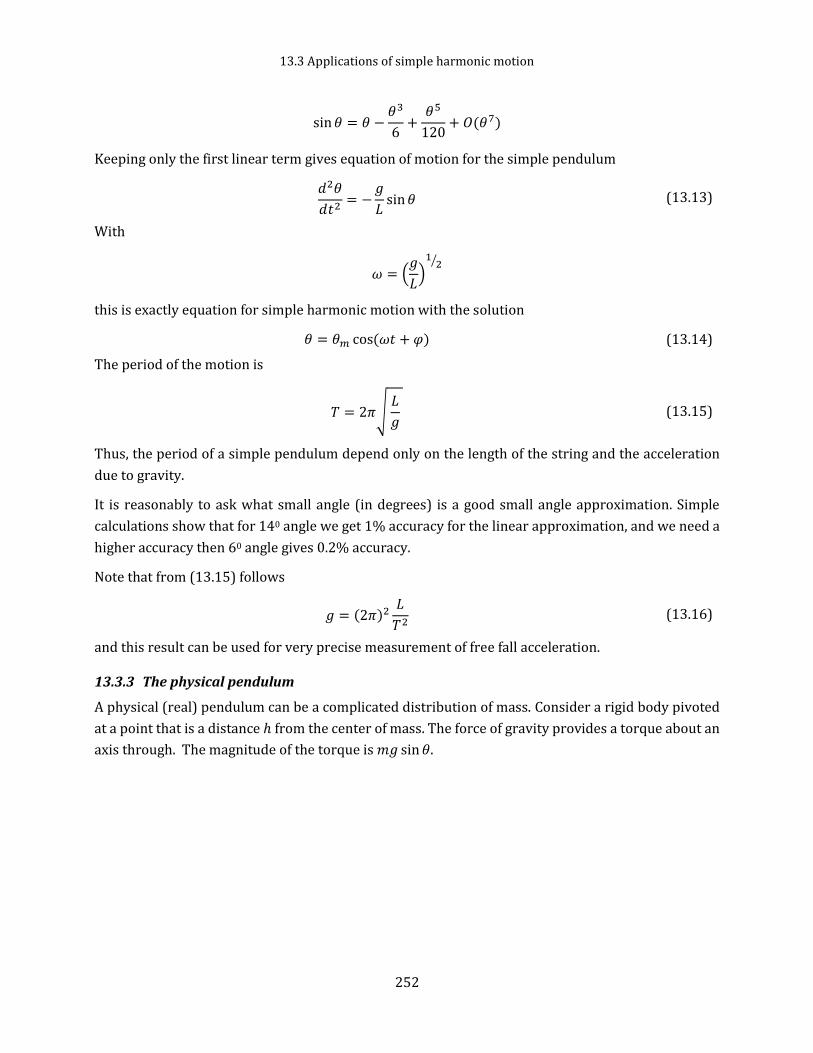
13.3 Applications of simple harmonic motion
252
sin 𝜃 = 𝜃 −𝜃3
6+
𝜃5
120+ 𝑂(𝜃7)
Keeping only the first linear term gives equation of motion for the simple pendulum
𝑑2𝜃
𝑑𝑡2= −
𝑔
𝐿sin 𝜃 (13.13)
With
𝜔 = (𝑔
𝐿)
12⁄
this is exactly equation for simple harmonic motion with the solution
𝜃 = 𝜃𝑚 cos(𝜔𝑡 + 𝜑) (13.14)
The period of the motion is
𝑇 = 2𝜋√ 𝐿
𝑔 (13.15)
Thus, the period of a simple pendulum depend only on the length of the string and the acceleration
due to gravity.
It is reasonably to ask what small angle (in degrees) is a good small angle approximation. Simple
calculations show that for 140 angle we get 1% accuracy for the linear approximation, and we need a
higher accuracy then 60 angle gives 0.2% accuracy.
Note that from (13.15) follows
𝑔 = (2𝜋)2𝐿
𝑇2 (13.16)
and this result can be used for very precise measurement of free fall acceleration.
13.3.3 The physical pendulum
A physical (real) pendulum can be a complicated distribution of mass. Consider a rigid body pivoted
at a point that is a distance ℎ from the center of mass. The force of gravity provides a torque about an
axis through. The magnitude of the torque is 𝑚𝑔 sin 𝜃.

13. Periodic Motion
253
Second newton’s law for rotation reads
𝐼𝑑2𝜃
𝑑𝑡2= 𝜏 = −𝑚𝑔ℎ sin 𝜃
Using, again, the small angle approximation we can rewrite the above equation
𝑑2𝜃
𝑑𝑡2= −
𝑚𝑔ℎ
𝐼𝜃
We can see that for small angular displacements the physical pendulum is follows simple harmonic
motion with
𝜔 = √𝑚𝑔ℎ
𝐼
and the period of oscillations
𝑇 = 2𝜋√𝐼
𝑚𝑔ℎ (13.17)
Equation (13.17) reduces to the period of a simple pendulum (13.15) when 𝐼 = 𝑚𝐿2, or when all the
mass is concentrated at the center of mass. This result can be used to measure the moment of inertia
of a flat rigid body if the location of the center of mass is known. The moment of inertia can be obtained
by measuring the period.
13.4 Simple harmonic motion and circular motion
The fact that the solution 𝑥(𝑡) = 𝐴 cos(𝜔𝑡 + 𝜑) contains cosines assumes that there might be
connection to a circular motion. Of course, such connection, if exists, is artificial because there are two
different kinds of motion. However, let us consider a uniform circular motion of a particle moving in
a circle of radius 𝑥𝑚 with a constant speed 𝑣. The angular position of a particle is 𝜃 that changes with

13.5 Damped and forced oscillations*
254
time as 𝜔𝑡 + 𝜙. Then 𝑑𝜃 𝑑𝑡⁄ = 𝜔 = 𝑣 𝑥𝑚⁄ . We know that there is an acceleration 𝑎 = 𝑣2 𝑥𝑚⁄ = 𝜔2𝑥𝑚
toward the center. At a given moment 𝑡 the positions along the 𝑥 and 𝑦 are
𝑥 = 𝑥𝑚 cos 𝜃 , 𝑦 = 𝑥𝑚 sin 𝜃
Using geometry and trigonometry we can write for the projection on the 𝑥 axis
𝑥(𝑡) = 𝑥𝑚 cos(𝜔𝑡 + 𝜙)
𝑣(𝑡) = −𝜔𝑥𝑚 sin(𝜔𝑡 + 𝜙)
𝑎(𝑡) = −𝜔2𝑥𝑚 cos(𝜔𝑡 + 𝜙)
which is exactly equations (13.5), (13.10) and (13.11).
Because uniform circular motion is so closely related mathematically to oscillatory up-and-down
motion, we can analyze oscillatory motion in a simpler way if we imagine it to be a projection of
something going in a circle.
13.5 Damped and forced oscillations*
So far we considered oscillations free from frictional forces. However, a spring or a pendulum
eventually stops because the mechanical energy is dissipated by friction (fluid/air resistance). Such
motion is said to be damped. For relatively slow speeds the frictional force of fluid resistance can be
expressed as
𝐹𝑑 = −𝑎𝑣
where 𝑎 is a damping coefficient. The minus sign indicates that the force opposes the motion.
13.5.1 Damped motion
We consider a body of mass 𝑚 attached to a spring and oscillating horizontally about its position of
equilibrium. Let 𝑥 be the horizontal distance of the body from the equilibrium position. Suppose that
the motion takes place in a medium whose resistance is proportional to the velocity. The differential
equation of motion becomes:
𝑚𝑑2𝑥
𝑑𝑡2= −𝑎
𝑑𝑥
𝑑𝑡− 𝑘𝑥 = 0
or with notations 2𝑏 = 𝑎/𝑚 and 𝜔02 = 𝑘/𝑚 we can write

13. Periodic Motion
255
𝑑2𝑥
𝑑𝑡2+ 2𝑏
𝑑𝑥
𝑑𝑡+ 𝜔0
2𝑥 = 0
There are two types of solutions depending on the value of 𝐷 = 𝑏2 − 𝜔02 < 0. Most interesting motion
happens when the coefficient of resistance 𝑏 is fairly small compared with the coefficient of
restoration 𝑘, so that 𝑏2 − 𝜔02 is negative: 𝑏2 − 𝜔0
2 = −𝜔′2.
Then the solution can be written in the form
𝑥(𝑡) = 𝐴𝑒−𝑏𝑡 cos(𝜔′𝑡 + 𝜑)
where
𝜔′ = √𝜔02 − 𝑏2
Here, 𝜔′ is the angular frequency of free vibrations, 𝐴 is the initial amplitude, and 𝜑 is the initial phase.
This formula represents damped oscillations, the speed of damping being characterized by the factor
𝑒−𝑏𝑡. In an interval of time equal to the period, the amplitude decreases in the ratio 𝑒−𝑏𝜏.
When 𝜔′ = 0, the condition is called critical damping. The system no longer oscillates but returns to
its equilibrium position without oscillation as
𝑥(𝑡) = 𝑒−𝑏𝑡(𝐶1 + 𝑥𝐶2)
where 𝐶1 and 𝐶2 are defined by initial conditions.
If 𝑏2 − 𝜔02 = 𝛾2 is positive, the solution is
𝑥(𝑡) = 𝐶1𝑒(−𝑏+𝛾)𝑡 + 𝐶2𝑒−(𝑏+𝛾)𝑡
Since we obviously have here 𝛾 < 𝑏, therefore 𝑥 tends to zero on indefinite increase of 𝑡 but the
system returns to equilibrium more slowly than with critical damping.

13.6 Examples
256
13.5.2 Forced oscillations and resonance
Assume that there is an additional external force 𝑓(𝑡) = 𝑓0 sin(𝜔𝑡) acting on the block. Then we can
modify the dumping equation as
𝑑2𝑥
𝑑𝑡2+ 2𝑏
𝑑𝑥
𝑑𝑡+ 𝜔0
2𝑥 = 𝑓0 sin(𝜔𝑡)
This differential equation can be solved either by variation of parameters or using the method of
undetermined coefficients. This subject belong to courses on ordinary differential equations. The
general solution can be written as
𝑥 = 𝐶1𝑒−𝑏𝑡 cos 𝛽𝑡 + 𝐶2𝑒−𝑏𝑡 sin 𝛽𝑡 +𝑓0
(𝜔02 − 𝜔2)2 + (2𝑏𝜔)2
{(𝜔02 − 𝜔2) sin 𝜔𝑡 − 2𝑏𝜔 cos 𝜔𝑡}
The solutions shows that, because an external force is driving it, the motion is not damped. The
external force provides the necessary energy to overcome the losses due to the retarding force. Note
that the system oscillates at the angular frequency 𝜔 of the driving force. For small damping, the
amplitude becomes very large when the frequency of the driving force is near the natural frequency
of oscillation. The dramatic increase in amplitude near the natural frequency 𝜔0 is called resonance.
13.6 Examples
Example 13-1
In what time after motion begins will a harmonically oscillating point be brought out of the
equilibrium position by half the amplitude? The oscillation period is 24 s and the initial phase is zero.
Answer: 4 s
Example 13-2
The initial phase of harmonic oscillation is zero. What fraction of the period will it take for the velocity
of the point be equal to half its maximum velocity? Answer t=(1/6)T

13. Periodic Motion
257
Example 13-3
A ball suspended from a thread 2 m long is deflected through an angle of 4 degrees and its oscillations
are observed. Assuming the oscillations to be undamped and harmonic, find the velocity of the ball
when it passes through the position of equilibrium. Check the solution by finding this velocity from
the equations of mechanics. Answer: 0.31 m/s
𝑣 = 𝜃0√𝑔𝑙
Example 13-4
A mass 𝑚 is connected to two springs of force constants 𝑘1 and 𝑘2 , In each case, the mass moves on
a frictionless table and is displaced from equilibrium and then released. Find the periods of motion
for both configurations
As small variation of the above problem: Find the period of
small vertical oscillations of a body with mass 𝑚 for the system
Example 13-5
How will the period of vertical oscillations of a load hanging on two identical springs change if instead
of tandem connection the springs are connected in parallel? Answer: The period will be halved.
Example 13-6
A particle of mass m is located in a unidimensional potential field where the potential energy of the
particle depends on the coordinate 𝑥 as 𝑈(𝑥) = 𝑈0(1 − cos 𝑎𝑥); 𝑈0 and 𝑎 are constants. Find the
period of small oscillations that the particle performs about the equilibrium position.
Answer: 2𝜋√𝑚 𝑎2𝑈0⁄
Solve the foregoing problem if the potential energy has the form

13.6 Examples
258
𝑈(𝑥) =𝑎
𝑥2−
𝑏
𝑥
where 𝑎 and 𝑏 are positive constants. Answer 4𝜋𝑎√𝑚𝑎 𝑏2 ⁄
Example 13-7
A body of mass 𝑚 fell from a height h onto the pan of a spring scale. The masses of the pan and the
spring are negligible, the spring coefficient is 𝑘. Having stuck to the pan, the body starts performing
harmonic oscillations in the vertical direction. Find the amplitude and the energy of these oscillations.
𝐴 =𝑚𝑔
𝑘√1 +
2𝑘ℎ
𝑚𝑔, 𝐸 = 𝑚𝑔ℎ +
1
2
𝑚2𝑔2
𝑘
(b) Solve the problem for the case of the pan having a mass 𝑀. Find the oscillation amplitude in this
case.
Example 13-8
A physical pendulum is positioned so that its center of gravity is above the suspension point. From
that position the pendulum started moving toward the stable equilibrium and passed it with an
angular velocity 𝜔. Neglecting the friction find the period of small oscillations of the pendulum.
Answer: 𝑇 = 4𝜋/𝜔
Example 13-9*
A pendulum clock is mounted in an elevator car which starts going up with a constant acceleration a,
with a < g. At a height h the acceleration of the car reverses, its magnitude remaining constant and the
elevator car goes another h to stop. Compare time measured by the pendulum clock to time measured
by not moving clock
𝑇𝑝𝑒𝑛𝑑 = 𝑇0 (√𝑔
𝑔 − 𝑎+ √
𝑔
𝑔 + 𝑎)
Example*
Imagine a shaft going all the way through the Earth from pole to pole along its rotation axis. Assuming
the Earth to be a homogeneous ball and neglecting the air drag, find: (a) the equation of motion of a
body falling down into the shaft; (b) how long does it take the body to reach the other end of the shaft;
(c) the velocity of the body at the Earth's center.
Answers:

13. Periodic Motion
259
𝑑2𝑦
𝑑𝑡2= −
𝑔
𝑅𝑦, 𝑇 = 𝜋√
𝑅
𝑔 42 𝑚𝑖𝑛, 𝑣 = √𝑔𝑅 = 7.9 𝑘𝑚/𝑠,
Example*
A mathematical pendulum 0.5 m long brought out of equilibrium deflects by 5 cm during the first
oscillation and by 4 cm during the second one (in the same direction). Find the time of relaxation, i.e.,
the time during which the amplitude of the oscillations decreases 𝑒 times, where 𝑒 is the base of
natural logarithms.
6.4 s.
Example*
A pendulum clock is mounted in an elevator car which starts going up with a constant acceleration a,
with a < g. At a height h the acceleration of the car reverses, its magnitude remaining constant. How
soon after the start of the motion will the clock show the right time again?
𝑡 = √2ℎ
𝑎
√1 + 𝜇 − √1 − 𝜇
1 − √1 − 𝜇, 𝜇 = 𝑎/𝑔
A pendulum clock is placed inside a rocket taking off vertically with acceleration a. What will be the
reading of the clock after the rocket fall back to the ground, if the engine worked for T seconds?
𝑇1 = 𝑇√1 + 𝑎/𝑔
???
A particle moves along the 𝑥 axis as 𝑥 = 2.7 cos 𝜋𝑡. Find the distance that the particle covers during
the time interval from t = 0 to 60 s. (both calculus and thinking)

14.1 Density and pressure
260
14 Fluids
It is impossible to imagine life without water and air. They are both fluids. The main property that
differentiates fluids from solids is that fluids do not maintain their own shape but conforms to
boundaries of a container in which we put them. In other words – a fluid is a substance that flows
because it will move under the shear. On molecular level it means that molecules in fluids are held
together by weak forces that are not strong enough to maintain a shape under gravity or other
external force.
14.1 Density and pressure
So far we mostly work with mass and force. Since fluids are extended substances we need to introduce
two properties of fluids. Such properties that they can vary from point to point inside that fluid.
First we need to define an equivalent of a force acting locally on a point in a fluid, and it is called
pressure. We express the average pressure 𝑝 as the normal force per unit area
𝑝 =Δ𝐹⊥
Δ𝐴
In the limit Δ𝐴 → 0
𝑝 =𝑑𝐹⊥
𝑑𝐴 (14.1)
Note that pressure is a scalar quantity. It does not have a specific direction inside a fluid because it
acts in all directions. At a surface the pressure acts perpendicular to the surface.
The SI unit of pressure is the pascal, where 1 pascal = 1Pa = 1 N/m2.

14. Fluids
261
Most common units for pressure in everyday life are millibars (mb) or atmosphere (atm) for
atmospheric pressure, pound per square inch (psi) in engineering (tire pressure).
Another local characteristic that we need is the density that we define as
𝜌 =Δ𝑚
Δ𝑉
or in the limit 𝛥𝑉 → 0
𝜌 =𝑑𝑚
𝑑𝑉.
For a fluid with uniform density (like water) we use
𝜌 =𝑚
𝑉 (14.2)
where 𝑚 and 𝑉 are the whole mass and volume of the fluid.
Density is also a scalar quantity. The SI unit of density is the kilogram per cubic meter (1 kg/m3). Note
that the density of a gas varies with pressure, (compressible fluids) but the density of a liquid (e.g.
water) does not (uncompressible fluid).
The density of air is about 1.21 kg/m3. It is interesting to estimate how many kg or lb of air in an
average classrooms. We may feel it is a very little number. Assume that a classroom has following
dimensions: 12 m deep, 8 m wide and 4 m tall. Than according to (14.2) 𝑚 = 𝜌𝑉 = 465 𝑘𝑔 (or
1024 lb) which is quite a large number!.
14.2 Hydrostatics
Hydrostatics is the theory of liquids at rest. When liquids are at rest, there are no shear forces. There
are two conclusions from this. First, the pressure stress is the same in all directions. Second, the
stresses are always normal to any surface inside the fluid. (Here we state both conclusions without
proof. But the proof is quite straightforward).
The pressure in a fluid may vary from place to place. From our experience we know that as we dive,
even in a swimming pool, we feel water pressure increases with depth.
14.2.1 Hydrostatic pressure
Let us analyze an effect of gravity on pressure in a fluid if the density 𝜌 of the fluid is considered
constant (it means liquid – uncompressible fluid).
Let us select a volume of the liquid contained within an imaginary boundaries. Let the cross-sectional
area of the top and bottom surfaces is 𝐴, and 𝑦1 and 𝑦2 are depths below the surface.
In case of a static equilibrium (hydrostatic) the sampled volume does not move, that if the net forces
in all directions are zero. We will concentrate on forces active in the vertical direction since there is
no gravity acting in the horizontal directions. Assume that the liquid pressure is 𝑝1 at 𝑦1 level and 𝑝2
at 𝑦2 level.

14.2 Hydrostatics
262
Then the force acting on the top surface of the volume is 𝐹1 = 𝑝1𝐴 and on the bottom surface if 𝐹2 =
𝑝2𝐴. The net force in the vertical direction is
𝐹𝑛𝑒𝑡 = 𝐹2 − 𝐹1 − 𝑚𝑔
The net force acting in the horizontal direction is zero (fluid is in equilibrium)
𝐹𝑅 + 𝐹𝐿 = 0
The mass of the liquid in the volume is 𝑚 = 𝜌𝑉 = 𝜌𝐴(𝑦1 − 𝑦2). (Note that both 𝑦1 and 𝑦2 are
negative). Then together with forces defined through the pressures
𝑝2𝐴 = 𝑝1𝐴 + 𝜌𝐴𝑔(𝑦1 − 𝑦2)
or
𝑝2 = 𝑝1 + 𝜌𝑔(𝑦1 − 𝑦2) (14.3)
If we seek for the pressure as a function of depth ℎ (where ℎ is positive) below the liquid surface, then
we choose 𝑝0 to be the atmospheric pressure at the surface (𝑦1 = 0) and (14.3) becomes
𝑝 = 𝑝0 + 𝜌𝑔ℎ (14.4)
and it is a constant in the static fluid for given ℎ.
We can apply the above analysis to a small change in the vertical position 𝑑𝑦. Then the change in
pressure will be 𝑝 + 𝑑𝑝 can be written as
𝑝 + 𝑑𝑝 = 𝑝 − 𝜌𝑔𝑑𝑦
where 𝑑𝑦.
𝑑𝑝
𝑑𝑦= −𝜌𝑔 (14.5)
If 𝜌 and 𝑔 are constants then
𝑑𝑝 = −𝜌𝑔𝑑𝑦
Integrating both parts

14. Fluids
263
∫ 𝑑𝑝𝑝
𝑝0
= −𝜌𝑔 ∫ 𝑑𝑦𝑦2
𝑦1
then 𝑝 − 𝑝0 = 𝜌𝑔(𝑦1 − 𝑦2) = 𝜌𝑔ℎ
and we come to equation (14.3) (remember that ℎ > 0 for depth).
14.2.2 Air pressure with height*
For gases (compressed fluids) the relation between pressure and depth (or altitude) is more
complicated because the gas density changes with pressure and temperature. Let us consider a
simplified model for air pressure as a function of height. Assume that air density is proportional to
pressure or 𝜌 = 𝛼𝑝 where 𝛼 is some constant. Then we can rewrite (14.5) as 𝑑𝑝 = 𝛼𝑝𝑔𝑑𝑦. Note that
we keep 𝑑𝑦 positive for height. Then equation becomes
𝑑𝑝
𝑝= 𝛼𝑔𝑑𝑦
Integrating both sides
∫𝑑𝑝
𝑝
𝑝
𝑝0
= 𝛼𝑔 ∫ 𝑑𝑦𝑦
𝑦0
gives ln 𝑝 − ln 𝑝0 = 𝛼𝑔(𝑦 − 𝑦0)
or
𝑝 = 𝑝0𝑒−𝛼𝑔ℎ (14.6)
where ℎ = 𝑦 − 𝑦0.
14.2.3 Pascal’s principle
From equation (14.4) follows that if we increase the pressure 𝑝0 at the top surface, then the pressure
𝑝 at any depth increases by exactly the same amount. A change in the pressure applied to an enclosed
incompressible fluid is transmitted undiminished to every point of the fluid and to the walls of its
container. This fact was recognized by Blaise Pascal in 17th century.
There is a very interesting and practical application based on this principle. Let us consider a
hydraulic lever.

14.2 Hydrostatics
264
Assume we applied a force of magnitude 𝐹1 to a piston of surface area 𝐴1 thus increasing pressure in
the liquid as 𝑝 = 𝐹1/𝐴1. The pressure is transmitted through a liquid to another piston of surface
area 𝐴2. Because the pressure must be the same on both sides 𝑝 = 𝐹1 𝐴1⁄ = 𝐹2 𝐴2⁄ and then
𝐹2 = 𝐹1
𝐴2
𝐴1
(14.7)
Equation (14.7) shows that the output force 𝐹2 must be greater than the input force if 𝐴2 > 𝐴1. When
we move the input piston downward by a distance 𝑑1, the output piston moves upward by a distance
𝑑2 so that the same volume of the incompressed liquid is displaced 𝑉 = 𝐴1𝑑1 = 𝐴2𝑑2
𝑑2 = 𝑑1
𝐴1
𝐴2
and it demonstrate that if 𝐴2 > 𝐴1 then the output piston moves a smaller distance. We can also
evaluate the work done on the input piston and the work done by the output piston on a load
𝑊 = 𝐹2𝑑2 = (𝐹1
𝐴2
𝐴1) (𝑑1
𝐴1
𝐴2) = 𝐹1𝑑1
which shows that they are equal. We do not get any energy advantage (sure we cannot!) but we have
a force-multiplying device. The number of applications for hydraulic levers are enormous.
14.2.4 Archimedes’ principle
Some 2000 years ago Archimedes stated that the magnitude of the buoyant force always equals the
weight of the fluid displaced by the object. The buoyant force acts vertically upward through the the
center of gravity of the displaced fluid.
We can derive Archimedes’ principle using Newton’s laws. In equilibrium (hydrostatic) the net force
acting on a portion of a fluid must be zero.
Let us consider an object insider a fluid.
The downward force on the top surface is
𝐹1 = 𝑝1𝐴
and the upward force on the bottom surface is

14. Fluids
265
𝐹2 = 𝑝2𝐴
The buoyant force on the object if a vector sum of the two forces
𝐹𝑏 = 𝐹2 − 𝐹1 = (𝑝2 − 𝑝1)𝐴
Using equation (14.4) we get
𝐹𝑏 = (𝑝1 + 𝜌𝑓𝑔ℎ − 𝑝1)𝐴 = 𝜌𝑓𝑔ℎ𝐴 = 𝜌𝑓𝑔𝑉𝑓 = 𝑚𝑓𝑔
or the buoyant force on an object in a fluid is
𝐹𝑏 = 𝜌𝑓𝑉𝑔 = 𝑚𝑓𝑔 (14.8)
where 𝜌𝑓 is the density of a fluid, and 𝑚𝑓 = 𝜌𝑓𝑉 is the mass of a fluid. This result is true for an object
with arbitrary shape (the proof is a bit longer).
For a body to float the buoyant force must exceed the force of gravity acting on that body.
Case 1: A completely submerged body.
Let us consider a body of mass 𝑚 and density 𝜌 that is completely submerged into a fluid. Then the
net vertical force acting on the body
𝐹𝑛𝑒𝑡 = 𝐹𝑏 − 𝑚𝑔 = 𝜌𝑓𝑉𝑔 − 𝜌𝑉𝑔 = (𝜌𝑓 − 𝜌)𝑉𝑔
Thus, for the body to float in a fluid its density must be less or equal to the density of the fluid 𝜌 ≤ 𝜌𝑓 .
If the density of the object is greater than the density of the fluid, then the buoyant force is less than
the downward force of gravity, and the object sinks.
If we place an object on a scale and measure its weight then we have 𝑤 = 𝑚𝑔. But is we do the same
inside a fluid than the reading is
𝑤𝑎𝑝𝑝 = 𝑤 − 𝐹𝑏
that is called an apparent weight.
𝑤𝑎𝑝𝑝 = 𝑚𝑔 − 𝜌𝑓𝑉𝑔 = 𝑚𝑔 − 𝜌𝑓
𝑚
𝜌𝑔 = 𝑚𝑔 (1 −
𝜌𝑓
𝜌)
Note that air has density different from zero (otherwise we would not be able to breath). Therefore
there is the buoyant force acting on all objects, including human bodies. Let us quickly estimate such
force assuming a volume of a human body to be 0.7m3. With the air density 1.21 kg/m3 we get
𝐹𝑏 = 8.3 𝑁 or about 1.9 𝑙𝑏.
Case 2: A partly submerged body.
In this case a body floats at a surface of a fluid, or the body is only partially submerged.
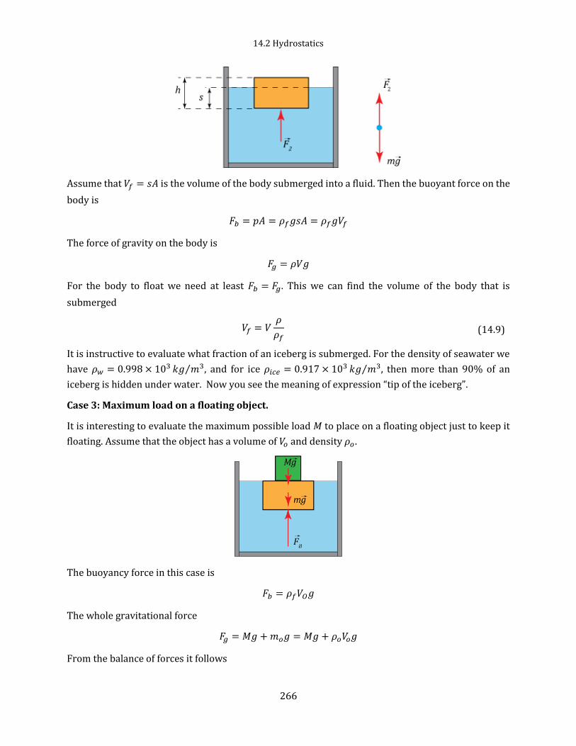
14.2 Hydrostatics
266
Assume that 𝑉𝑓 = 𝑠𝐴 is the volume of the body submerged into a fluid. Then the buoyant force on the
body is
𝐹𝑏 = 𝑝𝐴 = 𝜌𝑓𝑔𝑠𝐴 = 𝜌𝑓𝑔𝑉𝑓
The force of gravity on the body is
𝐹𝑔 = 𝜌𝑉𝑔
For the body to float we need at least 𝐹𝑏 = 𝐹𝑔. This we can find the volume of the body that is
submerged
𝑉𝑓 = 𝑉𝜌
𝜌𝑓 (14.9)
It is instructive to evaluate what fraction of an iceberg is submerged. For the density of seawater we
have 𝜌𝑤 = 0.998 × 10³ 𝑘𝑔 𝑚3⁄ , and for ice 𝜌𝑖𝑐𝑒 = 0.917 × 10³ 𝑘𝑔 𝑚3⁄ , then more than 90% of an
iceberg is hidden under water. Now you see the meaning of expression “tip of the iceberg”.
Case 3: Maximum load on a floating object.
It is interesting to evaluate the maximum possible load 𝑀 to place on a floating object just to keep it
floating. Assume that the object has a volume of 𝑉𝑜 and density 𝜌𝑜.
The buoyancy force in this case is
𝐹𝑏 = 𝜌𝑓𝑉𝑂𝑔
The whole gravitational force
𝐹𝑔 = 𝑀𝑔 + 𝑚𝑜𝑔 = 𝑀𝑔 + 𝜌𝑜𝑉𝑜𝑔
From the balance of forces it follows

14. Fluids
267
𝑀 = (𝜌𝑓 − 𝜌𝑜)𝑉𝑂
where 𝜌𝑓 is the density of the fluid.
14.2.5 Center of buoyancy and stability
There are two requirements for a body to be in equilibrium, namely 1) the vector sum of all the
external forces that act on the body, must be zero, and 2) the vector sum of all the external torques
that act on the body, measured about ANY possible point, must be zero.
So far, using simple geometries, our analysis was centered on the net vertical forces acting upon a
body. It is time to analyze the net torque created by gravity and the force of buoyancy.
The gravitational force on an extended body is the vector sum of the gravitational forces acting on the
individual elements (the atoms) of the body. In section 11.2 we proved that the center of gravity is
located at the center of mass as long as the object is in a uniform gravitational field.
The net buoyant force on a body immersed in fluid is also a vector sum of buoyant forces acting on
elementary (Δ𝐴 → 0) surfaces. It is possible to show (not in this course) that the center of buoyancy
(the point at which the net buoyancy force acts on the body) is equivalently the geometric center of
the submerged portion of the body. Or the center of buoyancy of an object is located at the point that
would be the center of mass of the displaced fluid.
Case 1: A completely submerged body.
For a completely submerged body of a uniform density its center of gravity is the same as the center
of buoyancy. Then the net torque is zero for any orientation of the body. We have neutral equilibrium.
However, if a body does not have uniform density then the outcome depends on relative locations of
the two centers. Let us consider an object of a spherical shape when its center of gravity is shifter
from the center of the sphere
If the center of gravity is located below the center of buoyancy, then after a small rotation the net
torque (around any point) works as a “restoring” torque by bringing the body back to its original
position of stable equilibrium. However if the center of gravity is above the center of buoyancy, then
a small deviation from the original position results in a net torque that rotates the body from its
unstable equilibrium to a stable position (that is different from the initial).

14.3 Hydrodynamics
268
Case 2: A partly submerged body.
For a floating body the situation is more complicated since the center of buoyancy usually shifts when
the body is rotated. Such a shift depends on the shape of the body and the orientation in which it is
floating.
Understanding physics of stability of floating objects is of paramount importance for engineering, like
shipbuilding.
On the figure we consider three situations for a partly submerged object (imagine it is a ship)
For the first situation (the center of gravity is below the center of buoyancy) a deviation from the
initial positions results in torques rotating the ship back (we have stable equilibrium here). For B)
and C) the center of gravity is located above the center of buoyancy. However, for B) situations, the
horizontal shift of the force of buoyancy is larger than for the force of gravity. Therefore the ship will
be back to its original upright position. For C) situation the center of gravity is so high that the center
of buoyancy is not shifted enough to restore the original position thus both torques rotate the ship in
the same direction resulting in capsizing of the ship.
Applying the same analysis to a pencil floating in water we can understand why pencils float only
horizontally unless we attach a weight to one of the ends.
14.3 Hydrodynamics
Modelling motion of fluids is one of most challenged problems in physics, including computational
challenges. To describe the motion of a fluid we need to describe its properties at every point. First,
at different points fluid is moving with different velocities. It means we must know the velocity vector
(the three components) at every point and for any time. However, the velocity is not the only property
that which varies from point to point. We need to deal with the variation of the pressure from point
to point. There may also be a variation of density from point to point. So the number of fields needed
to describe the complete situation will depend on how complicated the problem is.
In this section we are going to consider motion of a fluid at a lower level of complexity. We will focus
on the motion of an ideal fluid.

14. Fluids
269
1. We will reduce the complexity of our work by making the assumption that the density is a
constant – or the fluid is essentially incompressible. Putting it another way, we are supposing
that the variations of pressure are so small that the changes in density produced thereby are
negligible.
2. The flow is steady (laminar), such that the velocity of the fluid at each point does not change
with time.
3. We suppose that the viscosity of the liquid is unimportant. Viscosity characterizes internal
friction. This is a very strong approximation and it has almost nothing to do with real fluids.
John von Neumann characterized the theorist who made such analyses as a man who studied
"dry water”. However, even such idealized picture leads to understanding of some basic
principles of motion of fluids. Motion of fluids with viscosity is a subject of upper level
courses.
14.3.1 Conservation of mass
Let us consider a portion of a tube with variable cross section. For a common tube, fluid cannot
created or destroyed within the tube, and it cannot be stored. If a mass 𝑀of the fluid enters through
area 𝐴1 during some time interval, then the same mass leaves through area 𝐴2 during the same time
interval.
Since the volume can be written as 𝑉 = 𝐴𝑑𝑥 = 𝐴𝑣𝑑𝑡 where 𝑣 is the fluid’s speed, we get for the
conservation of mass
𝑀 = 𝜌1𝐴1𝑣1𝑑𝑡 = 𝜌2𝐴2𝑣2𝑑𝑡
or
𝜌1𝐴1𝑣1 = 𝜌2𝐴2𝑣2 = a constant (14.10)
The expression above states that the mass flow rate per unit time is constant
For uncompressible fluids (like water) 𝜌1 = 𝜌2 and then
𝐴1𝑣1 = 𝐴2𝑣2 = a constant (14.11)
or the volume flow rate is constant.

14.3 Hydrodynamics
270
14.3.2 Bernoulli’s equation
Normally Bernoulli’s equation is derived from a more general equation of motion of a fluid. Since it
involves using vector calculus we take an easier approach assuming from the beginning a steady flow
of a fluid. By steady flow we mean that at any one place in the fluid the velocity never changes. The
fluid at any point is always replaced by new fluid moving in exactly the same way. The velocity picture
always looks the same or �⃗� is a static vector field. A steady flow does not mean that nothing is
happening – atoms in the fluid are moving and changing their velocities. It only means that
𝜕�⃗�/𝜕𝑡 = 0
Then we can choose two areas in a non-uniform pipe where the speed of fluid is 𝑣1 in the first are and
𝑣2 in the second area do not change with time.
Now we are ready to apply energy consideration. The force exerted by the fluid is 𝑝𝐴 . The work done
by this force in a time 𝑡 is 𝑝𝐴Δ𝑥 = 𝑝Δ𝑉, where Δ𝑉 is the volume of the corresponding section. The
work done by pressure on fluid in the first section is positive
𝑊1 = 𝑝1Δ𝑉
but the work in the second section id negative because the fluid force opposes the displacement
𝑊2 = −𝑝2Δ𝑉
Considering pressure as a cause of an external force that changes kinetic and gravitational potential
energy of the fluid we can write
Δ𝐾 + Δ𝑈𝑔 = 𝑊1 + 𝑊2
Assuming that the mass of fluid is conserved, Δ𝑚 is our at the first area and Δ𝑚 is in at the second
area
1
2Δ𝑚𝑣2
2 −1
2Δ𝑚𝑣1
2 + Δ𝑚𝑔𝑦2 − Δ𝑚𝑔𝑦1 = 𝑝1Δ𝑉 − 𝑝2Δ𝑉
Using Δ𝑚 = 𝜌Δ𝑉 and rearranging the terms yields

14. Fluids
271
𝑝1 +1
2𝜌𝑣1
2 + 𝜌𝑔𝑦1 = 𝑝2 +1
2𝜌𝑣2
2 + 𝜌𝑔𝑦2 = a constant (14.12)
This is Bernoulli's theorem. The constant may in general be different for different flows; all we know
is that it is the same all along a given flow. The Bernoulli’s principle is in fact nothing more than a
statement of the conservation of energy. A conservation theorem such as this gives us a lot of
information about a flow without having to solve the detailed equations of motion.
Attentions: Bernoulli’s principle is valid only for incompressible and steady flow fluids with no
internal friction (no viscosity).
You can quickly test the Bernoulli principle by using two pieces of paper holding them close together
and trying to blow them apart. They actually come together. The reason, of course, is that the air has
a higher speed going through the constricted space between the sheets than it does when it gets
outside. The pressure between the sheets is lower than atmospheric pressure, so they come together
rather than separating.

14.4 Examples
272
14.4 Examples
* force on a vertical wall (calculus – integration)
*** see more in my handwritten notes
*** problems on ice in a glass of water, melting ice.
* water flowing from a water tank (find speed) F2-40-7
A friend asks you how much pressure is in your car tires. You know that the tire manufacturer
recommends 30 psi, but it's been a while since you've checked. You can’t find a tire gauge in the car,
but you do find the owner's manual and a ruler. Fortunately, you've just finished taking physics, so
you tell your friend, "I don’t know, but I can figure it out." From the owner's manual you find that the
car's mass is 1500 kg. It seems reasonable to assume that each tire supports one-fourth of the weight.
With the ruler you find that the tires are 15 cm wide and the flattened segment of the tire in contact
with the road is 13 cm long. What answer will you give your friend?
How many helium-filled toy balloons would be required to lift you? Take the size of an average helium
toy balloon to be 40 cm in diameter.
The three stooges (Moe, Larry, and Curly) make a log raft by lashing together oak logs of diameter 0.3
m and length 1.8 m. The total weight of the stooges is 480 lb.
a) How many logs will be needed to keep them afloat in fresh water?
b) What fraction of the raft will be above the water surface without the stooges on the raft?
c) Curly says that there is no point to make the raft since, as he read in a magazine, the average
density of a human body is less than the density of water. They would float anyway. Do you
agree or disagree with Curly? Provide a very good and supported answer.
Reference data for density: fresh water 1.0 g/cm3, wood (oak) 0.8 g/cm3.
A hurricane wind blows across a 6.0 m * 15.0 m flat roof at a speed of 130 km/h.
a) Is the air pressure above the roof higher, or lower than the pressure inside the house? Explain
b) What is the pressure difference?
c) How much force is exerted on the roof? If the roof cannot withstand this much force, will it
“blows in” or “blows out”?

14. Fluids
273
Water stands at a depth H in a large, open tank whose side walls are vertical. A hole is made in one of
the walls at a depth h below the water surface.
a) At what distance R from the foot of the wall does the emerging stream strike the floor
b) At what depth should the hole be placed to make the emerging stream strike the ground at the
maximum distance from the base of the tank?
Also find time to have water out of the tank
4.8. A liquid flows along a horizontal pipe AB (Fig. 6). The difference between the levels of the liquid
in tubes a and b is 10 cm. The diameters of tubes a and b are the same. Determine the velocity of the
liquid flowing along pipe AB.
Answer: 1.4 m/s.

15.1 Mechanical waves (physics behind the scene)
274
15 Waves
Most likely when you hear a word ‘weaves’ you think about water waves. If you had physics classes
before you may have some knowledge about sound waves, or even electromagnetic waves.
15.1 Mechanical waves (physics behind the scene)
In this chapter we are going to talk about mechanical waves that propagate in some physical medium
(liquid, gas, solid body). And sure the first question – what physics is behind mechanical waves?
In a physical medium atoms and/or molecules interact with their neighbors. Therefore, if we create
a perturbation in one point of physical medium, such perturbation propagates through the medium.
Imagine a long chain of balls connected by springs. If we provide a short perturbation (a kick) to a
spring on the left, then this perturbation will propagate in time from one ball to another.
We may reasonably guess that the speed of such perturbation is linked to the spring constants (the
larger the spring constant the faster the perturbation propagates) and to the mass of the blocks (the
larger the mass, the slower the speed of the propagation). Replacing balls and springs on atoms
provides a simple model that represents what is called longitudinal waves, when a traveling wave

15. Waves
275
causes the particles of the medium to move parallel to the direction of wave motion. Quite often a
continuous spring serves as a good model for longitudinal waves.
Now we kick one of the masses in a vertical direction. Then a travelling perturbation causes the
masses to move perpendicular to the wave motion.
Such wave is called a transverse wave. It is also possible to well model such a wave with a continuous
spring as
There are waves that are a combination of transverse and longitudinal displacements. For example,
water molecules on the surface of water, in which a wave is propagating, move in nearly circular
paths.
Each molecule is displaced both horizontally and vertically from its equilibrium position.
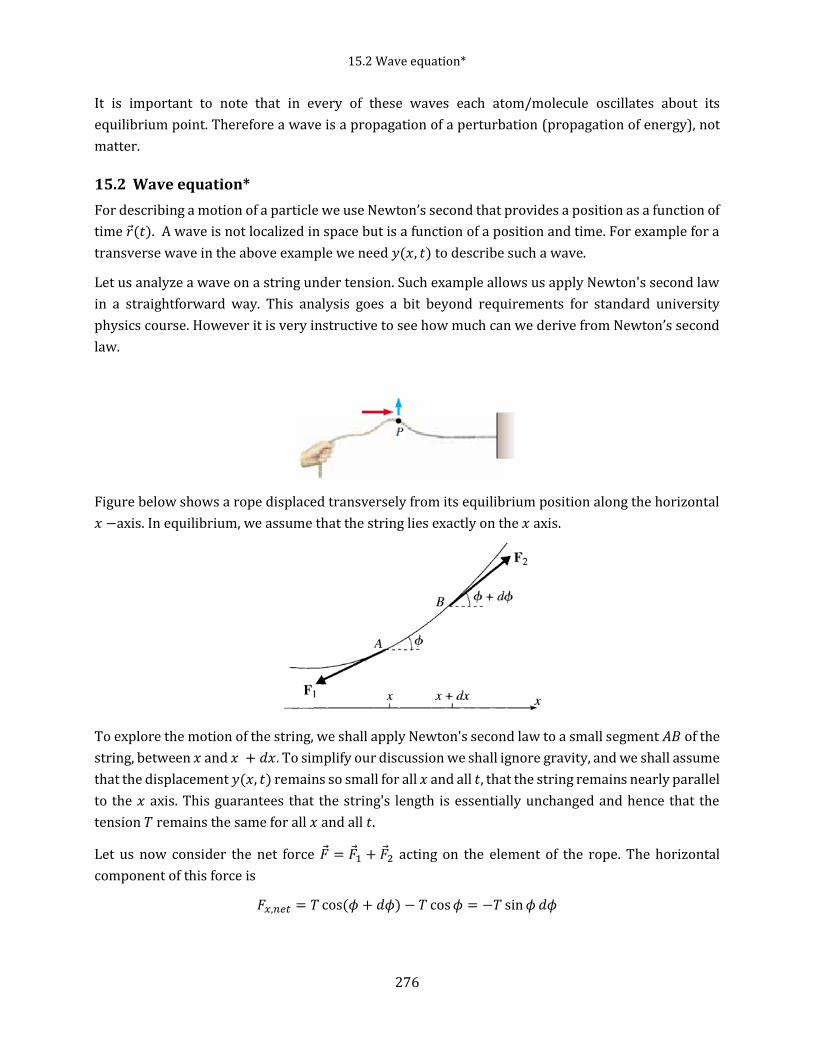
15.2 Wave equation*
276
It is important to note that in every of these waves each atom/molecule oscillates about its
equilibrium point. Therefore a wave is a propagation of a perturbation (propagation of energy), not
matter.
15.2 Wave equation*
For describing a motion of a particle we use Newton’s second that provides a position as a function of
time 𝑟(𝑡). A wave is not localized in space but is a function of a position and time. For example for a
transverse wave in the above example we need 𝑦(𝑥, 𝑡) to describe such a wave.
Let us analyze a wave on a string under tension. Such example allows us apply Newton's second law
in a straightforward way. This analysis goes a bit beyond requirements for standard university
physics course. However it is very instructive to see how much can we derive from Newton’s second
law.
Figure below shows a rope displaced transversely from its equilibrium position along the horizontal
𝑥 −axis. In equilibrium, we assume that the string lies exactly on the 𝑥 axis.
To explore the motion of the string, we shall apply Newton's second law to a small segment 𝐴𝐵 of the
string, between 𝑥 and 𝑥 + 𝑑𝑥. To simplify our discussion we shall ignore gravity, and we shall assume
that the displacement 𝑦(𝑥, 𝑡) remains so small for all 𝑥 and all 𝑡, that the string remains nearly parallel
to the 𝑥 axis. This guarantees that the string's length is essentially unchanged and hence that the
tension 𝑇 remains the same for all 𝑥 and all 𝑡.
Let us now consider the net force �⃗� = �⃗�1 + �⃗�2 acting on the element of the rope. The horizontal
component of this force is
𝐹𝑥,𝑛𝑒𝑡 = 𝑇 cos(𝜙 + 𝑑𝜙) − 𝑇 cos 𝜙 = −𝑇 sin 𝜙 𝑑𝜙

15. Waves
277
where 𝑇 is the magnitude of the tension in the rope. Since 𝜙 and 𝜙 + 𝑑𝜙 are both small, this is doubly
small, and 𝐹𝑥,𝑛𝑒𝑡 is negligible, consistent with our assumption that the motion is in the 𝑦 direction
only.
The 𝑦 component is
𝐹𝑦,𝑛𝑒𝑡 = 𝑇 sin(𝜙 + 𝑑𝜙) − 𝑇 sin 𝜙
That we can write (do you see the derivative of the sine function here?)
𝐹𝑦,𝑛𝑒𝑡 = 𝑇 cos 𝜙 𝑑𝜙
Certainly that the 𝑦 component is not negligible. Since 𝜙 is small we can replace cos 𝜙 by 1, and we
can write 𝑑𝜙 = (𝜕𝜙 𝜕𝑥⁄ )𝑑𝑥. The derivative is a partial derivative since 𝜙(𝑥, 𝑡) depends on 𝑥 and 𝑡.
Finally, again since 𝜙 is small, 𝜙 = 𝜕𝑦 𝜕𝑥⁄ , the slope of the string. Therefore,
𝐹𝑦,𝑛𝑒𝑡 = 𝑇𝑑𝜙 = 𝑇𝜕𝜙
𝜕𝑥𝑑𝑥 = 𝑇
𝜕2𝑦
𝜕𝑥2𝑑𝑥.
By newton’s second law, 𝐹𝑦,𝑛𝑒𝑡 = 𝑚𝑎𝑦, where 𝑎𝑦 is the acceleration
𝑎𝑦 =𝜕2𝑦
𝜕𝑡2
and mass is the mass of the segment 𝐴𝐵, equal to 𝜇𝑑𝑙 where 𝜇 is the linear density (mass per unit
length) and 𝑑𝑙 is the length of the segment 𝐴𝐵. For small angles 𝜙 we have 𝑑𝑥 = cos 𝜙 𝑑𝑙 = 𝑑𝑙. Thus
𝐹𝑦,𝑛𝑒𝑡 = 𝜇𝜕2𝑦
𝜕𝑡2𝑑𝑥
Equating the two expressions for the force we get for the equation of the string
𝜕2𝑦
𝜕𝑡2= (
𝑇
𝜇)
𝜕2𝑦
𝜕𝑥2 (15.1)
Introducing the notation
𝑣 = √𝑇
𝜇 (15.2)
where 𝑇 is the tension in our string and 𝜇 is its linear mass density. Then we can rewrite (15.1) as
𝜕2𝑦
𝜕𝑡2= 𝑣2
𝜕2𝑦
𝜕𝑥2 (15.3)
The equation of motion (15.3) is called the one-dimensional wave equation since its solutions are
waves traveling along the string. It is a partial differential equation, involving derivatives with respect
to 𝑥 and 𝑡. The constant 𝑣 has the dimensions of speed
[Tension
𝜇] =
[𝑀𝐿 𝑇2⁄ ]
[𝑀 𝐿⁄ ]= [
𝐿2
𝑇2] = speed2

15.3 Sinusoidal waves
278
and it is the speed with which the waves travel. Here we just note that this quantity depends on
internal properties of the medium, in this case the tension and mass density of a rope. The wave
equation (15.3) governs the motion of many different waves.
For waves on strings, 𝑦 represents the vertical displacement of the string. For sound waves, 𝑦
corresponds to displacement of air molecules from equilibrium or variations in either the pressure
or the density of the gas through which the sound waves are propagating.
Analysis of the wave equations (15.3) requires a good knowledge of partial differential equation. In
this chapter we are going to bring an important result following from (15.3) without proof.
Assume that at initial time 𝑡 = 0 the shape of the pulse can be represented as 𝑦 = 𝑓(𝑥). Then
measured in a stationary reference frame the wave function (that is the solution of the wave equation)
is
𝑦 = 𝑓(𝑥 − 𝑣𝑡)
for the pulse travelling to the right.
If the wave pulse travels to the left, the string displacement is
𝑦 = 𝑓(𝑥 + 𝑣𝑡)
For any given time 𝑡, the wave function 𝑦 as a function of 𝑥 defines a curve representing the shape of
the pulse at this time.
Hence, the wave speed is 𝑣 = 𝑑𝑥 𝑑𝑡⁄ .
Attention: The wave equation (15.3) describes propagation of a wave in space and time. Note that for
finding a unique solution for the wave we need both initial conditions (shape of the pulse or wave at
𝑡 = 0) and boundary conditions (real strings are finite in lengths and have ends).
15.3 Sinusoidal waves
An important special case of the solution (15.3) is the case that the function 𝑓 is sinusoidal. The
sinusoidal wave is the simplest example of a periodic continuous wave and can be used to build more
complex waves.
Assume that at time 𝑡 = 0 the wave function can be written as

15. Waves
279
𝑦(𝑥, 𝑡 = 0) = 𝐴 sin (2𝜋
𝜆𝑥) (15.4)
where the constant 𝐴 represents the wave amplitude and the constant 𝜆 is the wavelength. If the wave
moves to the right with a speed 𝑣, then the wave function at some later time 𝑡 is
𝑦(𝑥, 𝑡) = 𝐴 sin [2𝜋
𝜆(𝑥 − 𝑣𝑡)]. (15.5)
By definition, the wave travels a distance of one wavelength in one period 𝑇. Therefore, the wave
speed, wavelength, and period are related by the expression
𝑣 =𝜆
𝑇
Substituting this into (15.5) gives
𝑦(𝑥, 𝑡) = 𝐴 sin [2𝜋 (𝑥
𝜆 −
𝑡
𝑇)]
(15.6)
This form of the wave function shows the periodic nature of 𝑦. At any given time 𝑡 (a snapshot of the
wave), 𝑦 has the same value at the positions 𝑥, 𝑥 + 𝜆, 𝑥 + 2𝜆, and so on. Furthermore, at any given
position 𝑥, the value of 𝑦 is the same at times 𝑡, 𝑡 + 𝑇, 𝑡 + 2𝑇, and so on.
We can express the wave function in a convenient form by defining the angular wave number 𝑘
𝑘 =2𝜋
𝜆 (15.7)
and the angular frequency
𝜔 =2π
𝑇 (15.8)
Then we can write equation (15.6) in a standard form
𝑦(𝑥, 𝑡) = 𝐴 sin(𝑘𝑥 − 𝜔𝑡) (15.9)
If the wave were traveling to the left, we replace 𝑥 − 𝑣𝑡 by 𝑥 + 𝑣𝑡 in (15.5) or 𝑘𝑥 − 𝜔𝑡 by 𝑘𝑥 + 𝜔𝑡 in
equation (15.9).
If the vertical displacement 𝑦 is not equal to zero at 𝑡 = 0, then we can express the wave function with
a phase shift
𝑦(𝑥, 𝑡) = 𝐴 sin(𝑘𝑥 − 𝜔𝑡 + 𝜑)
where 𝜑 is the phase constant. This constant can be determined from the initial conditions.
Using the definitions for 𝑘, 𝜔 and frequency 𝑓 = 1 𝑇⁄ we can write 𝑣 in two more forms
𝑣 = 𝜆𝑓 =𝜔
𝑘.
We can show that the sinusoidal wave function (15.9) is a solution of the wave equation (15.3). The
appropriate derivatives are

15.4 Power transferred by a wave
280
𝜕2𝑦
𝜕𝑡2= −𝜔2𝐴 sin(𝑘𝑥 − 𝜔𝑡)
𝜕2𝑦
𝜕𝑥2= −𝑘2𝐴 sin(𝑘𝑥 − 𝜔𝑡)
Substituting these expressions into (15.3) gives
−𝜔2 = −𝑣2𝑘2
And since 𝑣 = 𝜔 𝑘⁄ we have an identity.
15.4 Power transferred by a wave
While a wave does not transfer matter, it does transfer energy. We will proceed with a model of a
wave on a string. Power is defined as
𝑃 = �⃗� ⋅ �⃗�
In the case of the string we can write
𝑃 = 𝐹𝑦𝑣𝑦 = −𝑇 sin 𝜙 𝜕𝑦
𝜕𝑡
where 𝑇 is the tension in the string. Since we work with small angles
sin 𝜙 ≈ tan 𝜙 =𝜕𝑦
𝜕𝑥
Then
𝑝 = −𝑇𝜕𝑦
𝜕𝑥
𝜕𝑦
𝜕𝑡
Calculating derivatives of the sinusoidal wave (15.9) gives
𝑃 = −𝑇[𝑘𝐴 cos(𝑘𝑥 − 𝜔𝑡)][−𝜔𝐴 cos(𝑘𝑥 − 𝜔𝑡)] = 𝑇𝜔𝑘𝐴2 cos2(𝑘𝑥 − 𝜔𝑡)
Earlier we got that 𝑣 = √𝑇 𝜇⁄ or 𝑇 = 𝑣2𝜇. Using also 𝑘 = 𝜔 𝑣⁄ we get
𝑃 = 𝑣2𝜇𝜔𝜔
𝑣𝐴2 cos2(𝑘𝑥 − 𝜔𝑡) = 𝜇𝑣𝜔2𝐴2 cos2(𝑘𝑥 − 𝜔𝑡).
The average power at any location 𝑥 is then
𝑃𝑎𝑣 =1
2𝜇𝑣𝜔2𝐴2 (15.10)
because the average value of cos2(𝑘𝑥 − 𝜔𝑡) is 1 2⁄ . This average is taken over an entire period of the
motion with 𝑥 held constant. This shows that the rate of energy transfer by a sinusoidal wave on a
string is proportional to the wave speed, the square of the frequency, and the square of the amplitude.

15. Waves
281
15.4.1 Wave intensity
We live in a three-dimensional world. Most types of waves (sound waves, seismic waves) carry energy
across all three dimensions. For such waves the intensity is a common characteristic that describes
energy transported by the wave in unit time, per unit area, across a surface perpendicular to the
direction of propagation. That is, intensity 𝐼 is average power per unit area. If a point source emits
waves uniformly in all directions, then the energy at a distance from the source is distributed
uniformly on a spherical surface of radius 𝑟 and area 𝐴 = 4𝜋𝑟2 and the intensity is
𝐼 =𝑃𝑎𝑣
4𝜋𝑟2 (15.11)
The intensity of a three-dimensional wave varies inversely with the square of the distance from a
point source. It is usually measured in watts per square meter.
15.5 Interference and reflection of waves
15.5.1 Superposition and interference
More often we encounter situations whet many waves are travelling through a medium. To analyze
such wave combinations, we use of the superposition principle. The principle states that if two or
more traveling waves are moving through a medium, the resultant wave function at any point is the
algebraic sum of the wave functions of the individual waves. Waves that obey this principle are called
linear waves and are generally characterized by small amplitudes. Waves that violate the
superposition principle are called nonlinear waves and are often characterized by large amplitudes.
Attention: One consequence of the superposition principle is that two traveling waves can pass
through each other without being destroyed or even altered.
The combination of separate waves in the same region of space to produce a resultant wave is called
interference. For two waves on a string we can then write
𝑦(𝑥, 𝑡) = 𝑦1(𝑥, 𝑡) + 𝑦2(𝑥, 𝑡) (15.12)
Mathematically, this additive property of wave functions follows from the form of the wave equation
(15.3). Specifically, the wave equation is linear; that is, it contains the function only to the first power.
As a result, if any two functions and satisfy the wave equation separately, their sum also satisfies it
and is therefore a physically possible motion. Because this principle depends on the linearity of the
wave equation and the corresponding linear-combination property of its solutions, it is also called the
principle of linear superposition.
When two waves cause increase in a resulting displacement then such superposition is called as
constructive interference. When the displacements caused by the two waves are in opposite
directions, we call such superposition as destructive interference.
There are very many interesting effects and applications of wave interference.

15.6 Sound waves
282
15.5.2 Reflection of waves
Let us consider a traveling wave when it encounters a change in the medium. For example a string
attached to a rigid support at one end. When the wave reaches the support, the wave undergoes
reflection that is, the wave moves back along the string in the opposite direction. And the reflected
wave is inverted.
If a wave reaches a boundary between two mediums then part of the incident wave is reflected and
part undergoes transmission, or some of the wave passes through the boundary. For example,
suppose a light string is attached to a heavier string. When a wave traveling on the light string reaches
the boundary between the two, part of the wave is reflected and inverted and part is transmitted to
the heavier string. The reflected pulse is inverted as in the case of the string rigidly attached to a
support. The following general rules apply to reflected waves: When a wave travels from medium 𝐴
to medium 𝐵 and 𝑣𝐴 > 𝑣𝐵 (that is, when 𝐵 is denser than 𝐴), the wave is inverted upon reflection.
When a wave travels from medium 𝐴 to medium 𝐵 and 𝑣𝐴 < 𝑣𝐵 (that is, when 𝐴 is denser than 𝐵), the
wave is not inverted upon reflection.
zzz: work more with this part (using the wave equation?)
15.5.3 Standing waves in a string
Let us look at a sinusoidal wave reflected by a fixed end of a string. If we continue shaking one end of
a string, a travelling wave will be reflected from the other end. Both the travelling and reflected waves
will interfere with each other. Usually it will be quite a noise of oscillations. However, if we vibrate
the string at one of right frequencies the two waves will interfere in such a way that a standing wave
will be formed. If the length of the string is 𝐿 then the condition for standing waves is
𝜆𝑛 =2𝐿
𝑛, 𝑛 = 1,2,3 …
where 𝜆 is the wavelength. In order to find the frequency 𝑓 of such vibrations we use 𝑓 = 𝑣 𝜆⁄ . Then
𝑓𝑛 =𝑣
𝜆𝑛= 𝑛
𝑣
2𝐿= 𝑛𝑓1
where 𝑓1 is the fundamental frequency.
zzz: add a figure + talk about nodes (and energy does not pass beyond nodes) +math representation
15.6 Sound waves
Sound waves are likely the most important of longitudinal waves in our lives. Sound waves may be
described as variations of pressure at various points. We still can employ the wave equation (15.3)
but in this case the speed of sound waves depends on the compressibility and inertia of the medium.
If the medium has a bulk modulus 𝐵 (bulk modulus measures the resistance of medium to changes in
their volume) and density 𝜌, then the speed of sound waves in fluids can be written as
𝑣 = √𝐵 𝜌⁄ (15.13)

15. Waves
283
Note that the speed of sound also depends on the temperature of the medium. It is good to know that
the speed of sound in air is approximately 343 m/s at temperature 200C.
The speed of sound in a solid material can be found from
𝑣 = √𝑌 𝜌⁄ (15.14)
where 𝑌 is Young’s modulus,
Mathematically a sinusoidal sound wave can be represented as the pressure variation
Δ𝑃 = 𝛥𝑃0 sin(𝑘𝑥 − 𝜔𝑡)
where 𝛥𝑃0 is the pressure amplitude, which is the maximum change in pressure from the equilibrium
value.
15.6.1 Intensity of sound; Decibels
The intensity of a wave, or the power per unit area, to be the rate at which the energy being
transported by the wave flows through a unit area A perpendicular to the direction of travel of the
wave. The human ear can detect a very wide range of intensities. For this reason it is convenient to
use a logarithmic scale, where the sound level 𝛽 is defined by the equation
𝛽 (in dB) = 10 log𝐼
𝐼0 (15.15)
where 𝐼0 is the intensity of some reference level taken to be at the “threshold of hearing” which is 𝐼0 =
1.0 × 10⁻¹² 𝑊 𝑚2⁄ . Thus, for example, the sound level of a sound intensity 𝐼 = 1.0 × 10⁻⁵ 𝑊 𝑚2⁄ will
be
𝛽 = 10 log1.0 × 10−5 𝑊 𝑚2⁄
1.0 × 10⁻¹² 𝑊 𝑚2⁄= 10 log 107 = 70 𝑑𝐵
that corresponds to a sound level of a busy street.
Note that the threshold of hearing corresponds to 0 𝑑𝐵.
15.6.2 Doppler Effect
When a source of sound is moving the frequency of the sound we hear is different than when the
source is at rest. This phenomenon is called the Doppler effect and occurs for all types of waves (not
only sound waves).
Case 1: Moving observer
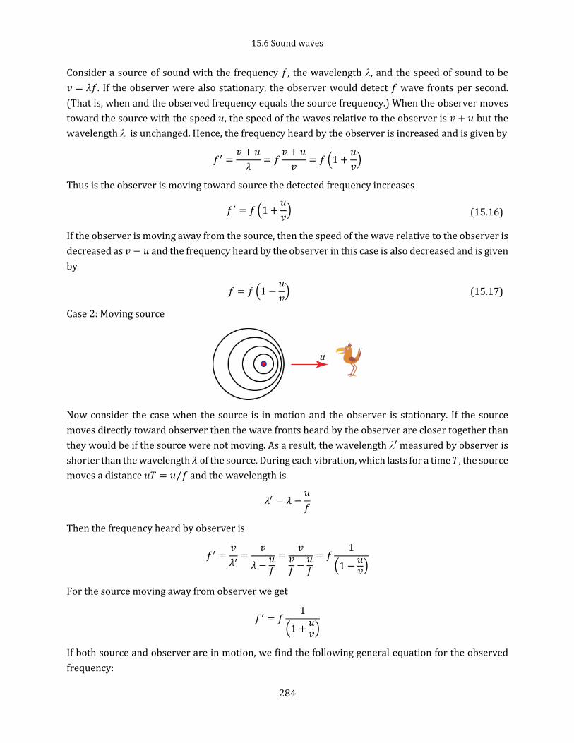
15.6 Sound waves
284
Consider a source of sound with the frequency 𝑓, the wavelength 𝜆, and the speed of sound to be
𝑣 = 𝜆𝑓. If the observer were also stationary, the observer would detect 𝑓 wave fronts per second.
(That is, when and the observed frequency equals the source frequency.) When the observer moves
toward the source with the speed 𝑢, the speed of the waves relative to the observer is 𝑣 + 𝑢 but the
wavelength 𝜆 is unchanged. Hence, the frequency heard by the observer is increased and is given by
𝑓′ =𝑣 + 𝑢
𝜆= 𝑓
𝑣 + 𝑢
𝑣= 𝑓 (1 +
𝑢
𝑣)
Thus is the observer is moving toward source the detected frequency increases
𝑓′ = 𝑓 (1 +𝑢
𝑣) (15.16)
If the observer is moving away from the source, then the speed of the wave relative to the observer is
decreased as 𝑣 − 𝑢 and the frequency heard by the observer in this case is also decreased and is given
by
𝑓 = 𝑓 (1 −𝑢
𝑣) (15.17)
Case 2: Moving source
Now consider the case when the source is in motion and the observer is stationary. If the source
moves directly toward observer then the wave fronts heard by the observer are closer together than
they would be if the source were not moving. As a result, the wavelength 𝜆′ measured by observer is
shorter than the wavelength 𝜆 of the source. During each vibration, which lasts for a time 𝑇, the source
moves a distance 𝑢𝑇 = 𝑢 𝑓⁄ and the wavelength is
𝜆′ = 𝜆 −𝑢
𝑓
Then the frequency heard by observer is
𝑓′ =𝑣
𝜆′=
𝑣
𝜆 −𝑢𝑓
=𝑣
𝑣𝑓
−𝑢𝑓
= 𝑓1
(1 −𝑢𝑣)
For the source moving away from observer we get
𝑓′ = 𝑓1
(1 +𝑢𝑣)
If both source and observer are in motion, we find the following general equation for the observed
frequency:
15. Waves
285
𝑓′ = (𝑣 ± 𝑢𝑂
𝑣 ∓ 𝑢𝑆) 𝑓 (15.18)
where the upper signs apply to motion of one toward the other, and the lower signs apply to motion
of one away from the other.
zzz More subjects: Musical instruments, interference of sound waves, beats, shock waves