1

University of São Paulo

“Luiz de Queiroz” College of Agriculture

Feed efficiency traits in Santa Inês sheep under genomic approaches

Amanda Botelho Alvarenga

Dissertation presented to obtain the degree of Master in

Science. Area: Animal Science and Pastures

Piracicaba

2017

3

Amanda Botelho Alvarenga

Animal Scientist

Feed efficiency traits in Santa Inês sheep under genomic approaches versão revisada de acordo com a resolução CoPGr 6018 de 2011

Advisor:

Prof. Dr. GERSON BARRETO MOURÃO

Dissertation presented to obtain the degree of Master in

Science. Area: Animal Science and Pastures

Piracicaba

2017

2

Dados Internacionais de Catalogação na Publicação

DIVISÃO DE BIBLIOTECA – DIBD/ESALQ/USP

Alvarenga, Amanda Botelho

Feed effiency traits in Santa Inês sheep under genomic approaches / Amanda

Botelho Alvarenga. - - versão revisada de acordo com a resolução CoPGr 6018 de

2011. - - Piracicaba, 2017.

66 p.

Dissertação (Mestrado) - - USP / Escola Superior de Agricultura “Luiz de

Queiroz”.

1. Associação genômica ampla 2. Consumo alimentar residual 3. Desequilíbrio

de ligação 4. Modelos de regressão Bayesianos 5. Seleção genômica I. Título

3

DEDICATION

I dedicate my dissertation work to my family. A special feeling of gratitude to my

loving parents, Luiz Cláudio Alvarenga and Andreia de Lima Botelho Alvarenga; my sister

Larissa Botelho Alvarenga; my grandfather and grandmother, Milton e Rosária; and to my

boyfriend, Guilherme Madureira.

Both of you have been my best cheerleaders and my biggest support.

4

ACKNOWLEDGEMENT

I would first like to thank God for all opportunities and the family and friends that

He gift for me. Second, I would like to acknowledge my dad (Luiz Cláudio Alvarenga), my

mom (Andreia de Lima Botelho Alvarenga), my sister (Larissa Botelho Alvarenga),

grandfather (Milton de Carvalho Botelho) and my grandmother (Rosária de Fátima Botelho

and Antônia Vilas Boas de Lima) for lovely family environmental, academic and personal

support during all my life. They always motivated me, believe and allow an important support

for me. I always will keep them in my heart and try my better to show that all are worthwhile.

For them, my love is unmeasured, infinity. Additionally, I would like to acknowledge all

people that compose the Botelho Alvarenga family.

Go on acknowledging my family, I also would like to thank my boyfriend

(Guilherme Madureira) and Madureira family. They were very important in the introduction

of Piracicaba’s life and now, such as Botelho Alvarenga family, are essential in my life. In

special, I would like to thank the Guilherme Madureira for daily support, advice and loving. I

must express my very profound gratitude to my parents, sister and to my boyfriend for

providing me with unfailing support and continuous encouragement throughout my years of

study and through the process of researching and writing this dissertation. This

accomplishment would not have been possible without them. Thank you.

I would like to thank my uncle, graduation's advisor, and academic advisor for all

life, Renato Ribeiro de Lima of the Federal University of Lavras (UFLA, Lavras, Minas

Gerais, Brazil). Until today, he directs me in my academic choices.

I thank the 'magnificent' "Luiz de Queiroz" College of Agriculture (ESALQ- USP,

Piracicaba, São Paulo, Brazil) for hosting and allowing me to be part of its academic

community, which in this environment is full of relevant and competent people in their areas

of research. In special, I would like to thanks professors of Animal Science, Statistics, and

Genetics department for all instructions and knowledge.

During the master’s time, I met important people that composed my formation

academic, as well as personal. First, thank you Professor Doctor Gerson Barreto Mourão, my

dissertation advisor at ESALQ for the opportunity to do my master' degree at the relevant

program in Animal Science and Pastures. Prof. Mourão was always open whenever I had new

ideas or problems. In special, I would like to thank the Barreto Mourão family (Luciana,

Giovanna and Gabriel) for receiving me so well at Piracicaba city.

5

Second, I thank my friends: Anna Rita Santos, Eula Regina Carrara, Fátima

Bogdanski, Gabriela Rocha, Gregori Rovadoscki, Mayara Salvian, Marie F. Laborde, Thais

Fagundes Matioli, Juliana Petrini and Vamilton Franzo. Thank you for nice days, advice, help

in analyses, to make e-mails, for the popcorn and bread with mortadella' moments, and

friendship. In special, I would like to acknowledge Juliana Petrini, my co-advisor. She

supported me in all analyses present in this dissertation, in theoretical information, writing

section and academic councils. Additionally, I would like to thanks, Eula Regina Carrara for

the great friendship.

I would also like to acknowledge Gota Morota and Matthew L. Spangler at

Department of Animal Science, University of Nebraska (UNL, Lincoln, NE, USA) by

contribution as reader and analyses of this dissertation, and I am gratefully indebted to him

very valuable comments on this dissertation.

I would also like to thank the experts who were involved in the validation survey for

this research project: Luiz Lenhmann Coutinho (and Coutinho’s lab), Aline Silva Mello

Cesar, Luis Fernando Batista Pinto, and Gleidson Giordano Pinto de Carvalho. Without their

participation and input, the survey could not have been successfully conducted.

Finally, I would like to thank São Paulo Research Foundation (FAPESP- Fundação

de Amparo à Pesquisa do Estado de São Paulo; process: 2015/25024-5 and 13/04504-3,

Brazil), by supported this work. We are indebted to the Federal University of Bahia (UFBA,

Salvador, Bahia, Brazil) for the partnership to sheep production and Biotechnology Lab of

Professor Luiz Lehmann Coutinho (ESALQ- USP) for support in genotyping.

6

SUMMARY

RESUMO ................................................................................................................................... 7

ABSTRACT ............................................................................................................................... 8

1. INTRODUCTION ................................................................................................................. 9

Reference ................................................................................................................................. 11

2. LINKAGE DISEQUILIBRIUM IN Ovis aries, SANTA INÊS BREED ............................ 13

Abstract .................................................................................................................................... 13

2.1 Introduction ........................................................................................................................ 13

2.2 Methods .............................................................................................................................. 15

2.3 Results and Discussion....................................................................................................... 18

2.4 Conclusion ......................................................................................................................... 26

Reference ................................................................................................................................. 27

3. GENOME-WIDE ASSOCIATION AND SYSTEMS GENETIC ANALYSES OF FEED

EFFICIENCY TRAITS IN SHEEP ......................................................................................... 31

Abstract .................................................................................................................................... 31

3.1 Introduction ........................................................................................................................ 31

3.2 Methods .............................................................................................................................. 33

3.3 Results ................................................................................................................................ 36

3.4 Discussion .......................................................................................................................... 38

Reference ................................................................................................................................. 44

4. GENOMIC SELECTION FOR RESIDUAL FEED INTAKE USING A SMALL OVINE

POPULATION......................................................................................................................... 47

Abstract .................................................................................................................................... 47

4.1 Introduction ........................................................................................................................ 47

4.2 Methods .............................................................................................................................. 49

4.3 Results and Discussion....................................................................................................... 52

4.4 Conclusion ......................................................................................................................... 55

Reference ................................................................................................................................. 56

5. FINAL CONSIDERATIONS .............................................................................................. 59

SUPPLEMENTARY FIGURES .............................................................................................. 61

SUPPLEMENTARY TABLES ............................................................................................... 63

7

RESUMO

Eficiência alimentar em ovinos da raça Santa Inês sob abordagem genômica

A seleção com base nos valores genéticos genômicos preditos pode

aumentar substancialmente a taxa de ganho genético em animais por meio do

aumento da acurácia de predição e redução do intervalo de gerações,

especialmente para características de difícil e/ou onerosa mensuração, como

eficiência alimentar. A eficiência alimentar é uma das características mais

importantes na produção animal devido principalmente aos seus impactos

econômicos e ambientais. Muitas métricas representam a eficiência alimentar, por

exemplo: a relação do ganho de peso e consumo alimentar (EA), a proporção do

consumo alimentar e ganho de peso (CA) e o consumo alimentar residual (CAR).

Em ovinos, nenhum estudo com o objetivo de buscar variantes genéticas ou

verificar a acurácia do valor genético genômico estimado para eficiência alimentar

foi publicado. Adicionalmente, antes de aplicar a informação genômica, é

necessário compreender e caracterizar a estrutura da população, como por meio do

desequilíbrio de ligação (LD). O estudo de associação genômica (GWAS) e

seleção genômica (GS) consideram o LD entre marcador e a mutação causal. Com

base nas considerações acima, o objetivo deste estudo foi mapear o LD em

ovinos, caracterizado pela raça ovina Santa Inês; localizar variantes genéticas para

as características de eficiência alimentar (EA, CA e CAR) utilizando a abordagem

GWAS; e verificar a acurácia da estimação dos valores genéticos genômico para o

CAR. No total, foram coletadas 396 amostras (animais) do músculo Longissimus

dorsi, para posterior genotipagem utilizando o painel de alta densidade (Illumina

High-Density Ovine SNP BeadChip®), compreendendo 54.241 SNPs. O banco

fenotípico é composto por 387 animais. O LD médio entre marcadores adjacentes

para duas métricas de LD, r² e |D'|, foram 0,166 e 0,617, respectivamente. O grau

de LD estimado foi menor que o relatado em outras espécies e foi caracterizado

por blocos de haplótipos curtos. Consequentemente, para as análises genômicas

são recomendados painéis de marcadores de alta densidade. No GWAS, foram

encontrados muitos marcadores associados aos fenótipos, em especial, à

característica CAR. Alguns genes candidatos foram relatados neste estudo,

destacando-se o NRF-1 (fator respiratório nuclear 1), que controla a biossíntese

mitocondrial, o processo mais importante responsável por grande parte da

produção de energia. Finalmente, verificamos a acurácia do valor genético

genômico estimado para o CAR usando modelos de regressão Bayesiana, e

encontramos baixos valores para acurácia (0,033 a 0,036) o que pode ser

explicado pelo baixo grau de relacionamento entre os indivíduos e tamanho

reduzido da população de treinamento.

Palavras-chave: Associação genômica ampla; Consumo alimentar residual;

Desequilíbrio de ligação; Modelos de regressão Bayesianos;

Seleção genômica

8

ABSTRACT

Feed efficiency traits in Santa Inês sheep under genomic approach

The selection on genetic values predicted from markers could

substantially increase the rate of genetic gain in animals by increasing accuracy of

prediction and reducing generation interval, especially for difficult to measure

traits, such as feed efficiency. Feed efficiency is the most important trait in

animal production due to its impacts on cost of production and environmental

factors. Many metrics measure the feed efficiency, such as ratio of gain to feed

(FER), the ratio of feed to gain (FCR) and residual feed intake (RFI).

Nevertheless, in ovine, no study with the aim of understand the genetic variants or

the accuracy of genomic estimated breeding value (GEBV) for feed efficiency

traits was published yet. Moreover, before to apply the genomic information, it is

necessary to understand and characterized the population structure, for instance,

by linkage disequilibrium (LD). Both genome-wide association studies (GWAS)

and genomic selection (GS) leverage LD between marker and causal mutation.

Based on the above considerations, the aim of this study was to map LD in ovine,

characterized by Brazilian Santa Inês sheep; to search genetic variants for feed

efficiency traits (FER, FCR and RFI) through GWAS; and to verify the accuracy

of GEBV for RFI. In total, 396 samples (animals) of Longissimus dorsi muscle

were collect. A high-density panel of SNP (Illumina High-Density Ovine SNP

BeadChip®) comprising 54,241 SNPs was used to obtain the genotyping data.

The phenotype data was comprised of 387 animals. The average LD between

adjacent markers for two LD metrics, r² and |D’|, were 0.166 and 0.617,

respectively. The degree of LD estimated was lower than reported in other species

and it was characterized by short haplotype blocks. Consequently, for genomic

analyses, high-density panels of marker are recommended. Many markers were

associated to feed efficiency traits in GWAS, mainly to RFI trait. Few candidate

genes were reported in this study, highlighting NRF-1 (nuclear respiratory factor

1), which controls mitochondrial biosynthesis, the most important process

responsible by a great fraction of the produced energy. Finally, we verified the

accuracy of GEBV for RFI using few Bayesian regression models, and we found

low accuracy, ranging from 0.033 (BayesB with 𝜋=0.9912) to 0.036 (BayesA),

which might be explained by the low relationship among animals and small

training population.

Keywords: Bayesian regression models; Genome-wide association study;

Genomic selection; Linkage disequilibrium; Ovine; Residual feed

intake

9

1. INTRODUCTION

The ovine production is the promising activity of agriculture because the

consumption of ovine meat had increased, especially in Brazil. Brazil is a promising producer

due to many advantages, such as extension area to production, tropical weather, and important

agriculture area for family farmers, due to ovine be small animals, consequently, easy

management.

However, Brazil’ ovine production does not supply the intern consumption and not

highlight in world exportation and production, such as bovine (first position in exportation),

chicken (first position in exportation) and pig (fourth position in exportation). The ovine

population on the 2014 year comprised of 17.6 million of heads, a smaller population

compared with Australia (72.6 million head) and New Zealand (29.8 million head), the two

biggest global exporter countries 1. Techniques to optimize the ovine production might be a

workaround to turn the ovine production more attractive to farmers; consequently, afford to

increase the sheep production and highlight it in the world trade.

An important trait that affects livestock production is the efficiency to convert the

feed intake into the final product. More efficient animals reduce the cost of production

because they require less feed (kilograms- kg) to yield a same amount of final product, for

example, carcass (kg) 2. Additionally, improving the animal’s efficiency might reduce the

methane liberation, allowing a more sustainable productive chain by the proper use of natural

resources, and consequently, reducing environmental impacts 2.

Many measures can represent the animal efficiency, such as the ratio between the

gain of weight and feed intake (feed efficiency- FER), the ratio between feed intake and

weight gain (feed conversion ratio- FCR) and residual feed intake (RFI). The FER and FCR

traits can result in overestimation of efficiency because they do not account the food needed

for maintenance 3. Moreover, FER and FCR can select more efficient animals concomitantly

to heavier animals 4,5

. In animal production, there is a threshold for weight or weight gain that

is economically advantageous; up to it might be an unsustainable economic chain. In this

context, the RFI was proposed as a feed efficiency trait that is independent of body weight

and weight gain 3. RFI or net feed intake is the difference between observed feed consumption

and expected feed consumption, being the expected feed consumption adjusted for average

daily gain (ADG) and metabolic mid-point weight (metabolicMIDWT). Consequently, the RFI

is a residual, which in the statistical process is independent of predictors (ADG and

metabolicMIDWT).

10

All these efficiency traits had medium to high heritability 3–5

, and therefore, it is

possible to use animal breeding as a tool to accumulative improve animal’s efficiency.

However, the use of genetic selection for efficiency traits is limited due to cost and difficulty

related to the measurement of such traits 6.

The use of genomic information can help in the genetic evaluation for these difficult

to measure traits, as cited above, as well as improve the accuracy due to the incorporation of

more information into the model, consequently, 8-38% extra genetic gain 7. This kind of data

allows inference about the genetic structure of the trait and of the population under selection,

being applied in the genomic selection (GS).

GS is an approach which uses genome-wide markers simultaneously to predict

breeding values 8. During the selection process, alleles favorable to the traits of interest are

selected directly or indirectly. In GS, we can select animals observing the favorable

polymorphism directly, based on its effect previously estimated. Generally, a genotyping

panel is used in GS. Because these commercial panels contain only a sample of the

polymorphisms present in the genome, genomic analyses leverage on the linkage

disequilibrium (LD) between the polymorphism present into the panel (SNP - single

nucleotide polymorphism) and the causal mutation 9,10

. Therefore, GS works by selecting

animals for hundreds of thousands of random markers simultaneously, assuming that the

majority of the causal mutations is in LD with such markers 8.

LD is defined as a stochastic dependence between alleles at two loci 11

. Previously to

any genomic study, it is important to map the LD of the breed of interest, because it can

change due to population structure (selection, migration, recombination rate) 10

. Since LD can

be an indicative of the segregation behavior of alleles, it enables to define the density of the

genotyping panel necessary to achieve a certain accuracy of prediction and to determine the

threshold time that the marker effects should be updated.

From the knowledge about population LD, it is possible to apply genomic

information optimally. Before GS, is necessary to estimate genetic marker effects in a

genome-wide association study (GWAS). GWAS also allows a genetic study about the

process that involves the trait under study, its genetic control. This study allows identifying

candidate genes related to the trait, through the verification of significantly markers associated

with the phenotype. Moreover, GWAS is the first step for other studies that aim to find the

causal mutation and genes that control the trait.

For performance the genomic approaches, we had chosen uses the Bayesian

regression approach. The first motivation is the increase in accuracy using Bayesian methods.

11

Using best linear unbiased prediction model an accuracy was 0.73, although using Bayesian

methods increased this accuracy to 0.85, even when the prior was not correct 8.

Therefore, despite the importance of the genomic approach as a tool to understand

the genetic control of traits of economic interest and also to optimize their genetic evaluation

and selection, we were not able to find studies that use genomic information in the animal

breeding for feed efficiency in ovine populations. Therefore, the aims in this study were: to

map the LD of Brazilian Santa Inês breed by using a genotyping panel of SNP; to develop the

first study involving the comprehension of the genetic control of feed efficiency in an ovine

population using GWAS approach; and finally, to verify the accuracy of GS for RFI in a

small population, as happen to many other breeds or species. The RFI was chosen for GS

analysis because it presented in this and other studies high accuracy and more advantages in

comparison to the both traits cited. The breed chosen to represent the study was the Santa Inês

breed because it is the most important ovine breed farming in Brazil. The Santa Inês is a

tropically adapted breed, with desirable characteristics for meat production and reproductive

efficiency. Moreover, this breed was formed by the non-systematic crossing of the Somali,

Bergamasca, and Morada Nova breeds 12

; potentially allowing inferences based on these

results on other breeds.

REFERENCES

1. FAO. Food and Agriculture Organization of the United Nations. http://www.fao.org/home/en/

(2017).

2. Basarab, J. a. et al. Residual feed intake and body composition in young growing cattle. Can. J.

Anim. Sci. 83, 189–204 (2003).

3. Koch, R. M., Swiger, L. A., Chambers, D. & Gregory, K. E. Efficiency of feed use in beef cattle.

J. Anim. Sci. 22, 486–494 (1963).

4. Archer, J. a, Arthur, P. F., Herd, R. M., Parnell, P. F. & Pitchford, W. S. Optimum postweaning

test for measurement of growth rate , feed intake , and feed efficiency in British breed cattle. J.

Anim. Sci. 75, 2024–2032 (1997).

5. Arthur, P. F., Renand, G. & Krauss, D. Genetic and phenotypic relationships among different

measures of growth and feed efficiency in young Charolais bulls. Livest. Prod. Sci. 68, 131–139

(2001).

6. Almeida, R. Consumo e eficiência alimentar de bovinos em crescimento. (2005).

7. Meuwissen, T. H. E. & Goddard, M. E. The use of marker haplotypes in animal breeding schemes.

Genet. Sel. Evol. 28, 161–176 (1996).

8. Meuwissen, T. H. E., Hayes, B. J. & Goddard, M. E. Prediction of total genetic value using

genome-wide dense marker maps. Genetics 157, 1819–1829 (2001).

9. Lu, D. et al. Linkage disequilibrium in Angus, Charolais, and Crossbred beef cattle. Front. Genet.

3, 1–10 (2012).

12

10. Miller, J.M.; Poissant, J.; Kijas, J.W.; Coltman, D.w., the I. S. G. C. A genome-wide set of SNPs

detects population substructure and long range linkage disequilibrium in wild sheep. Mol. Ecol.

Resour. 314–322 (2011). doi:10.1111/j.1755-0998.2010.02918.x

11. Khatkar, M. S. et al. Extent of genome-wide linkage disequilibrium in Australian Holstein-

Friesian cattle based on a high-density SNP panel. BMC Genomics 9, 187 (2008).

12. ARCO. Assistência aos rebanhos de criadores de ovinos - Associação Brasileira de Criadores de

ovinos. http://www.arcoovinos.com.br/index.php (2017).

13

2. LINKAGE DISEQUILIBRIUM IN Ovis aries, SANTA INÊS BREED

Amanda Botelho Alvarenga1, Gregori Alberto Rovadoscki

1, Juliana Petrini

1, Luiz

Lehmann Coutinho1, Gota Morota², Matthew L. Spangler², Luís Fernando Batista Pinto

3,

Gleidson Giordano Pinto de Carvalho3, & Gerson Barreto Mourão

1*

1 Department of Animal Science, University of São Paulo (USP) / Luiz de Queiroz College of

Agriculture (ESALQ), Piracicaba, SP, Brazil

2 Department of Animal Science, University of Nebraska, Lincoln, NE, USA

3 Department of Animal Science, Federal University of Bahia (UFBA), Salvador, BA, Brazil

ABSTRACT

Linkage disequilibrium (LD) is defined as a stochastic dependence between alleles at

two loci. Quantitative genetics analysis such as genome-wide association studies or genomic

selection (GS) leverages LD between the marker and the causal mutation. The objectives of

this study were to evaluate the extent of LD in ovine, using the Santa Inês breed, and infer the

minimum number of markers required to reach reasonable prediction accuracy in GS. In total,

38,168 SNPs and 395 samples were used for analysis. The overall mean LD between adjacent

marker pairs measured by r² and |D’| were 0.166 and 0.617, respectively. LD values between

adjacent marker pairs ranged from 0.135 to 0.194 for r² and from 0.568 to 0.650 for |D'| across

all chromosomes. The average r² between all pairwise SNPs on each chromosome was 0.018.

SNPs with distance between 0.10 to 0.20 Mb showed the average r² equal to 0.1033. The

identified haplotype blocks consisted of two to twenty-one markers. In addition, the estimates

of average inbreeding coefficient and effective population size were 0.04 and 96, respectively.

We also found a tendency for relationships between the extent of linkage disequilibrium and

both effective population size and inbreeding coefficient. The degree of LD estimated in this

study was lower than that reported in other species and it was characterized by short

haplotype blocks. Overall, our results suggest that the use of a higher density SNP panel is

recommended for the implementation of GS in ovine.

Keywords: Effective population size; Haplotype blocks; Medium-density SNP panel;

Inbreeding coefficient

2.1. Introduction

Genomic information is currently used in animal breeding programs to enable

selection for difficult to measure traits as well as to increase the understanding of genetic and

biological causes underlying phenotypic variation. Genomic selection (GS) is an approach

which uses genome-wide markers simultaneously to predict breeding values 1. This approach

excels in increasing genetic gains when pedigree-based selection is suboptimal 1, which is the

14

case of traits with low heritability. For instance, GS based on simulated data showed an

increase in reliability of breeding values for young animals when using genomic (greater than

60%) versus parent average (32%) information, equivalent to approximately 20 offspring 2.

Furthermore, genetic gain can be increased using genomic information by shortening the

generation interval 1.

Alternatively, genetic markers scattered across the genome offers an opportunity to

conduct genome-wide association studies (GWAS) to characterize genes underlying genetic

variation for traits of interest.

The success of GS and GWAS are dependent of linkage disequilibrium (LD) or

gametic disequilibrium between the markers and causal mutations 3 because generally the

former is observed but not the latter. The LD between a marker and a causal mutation can be

considered as the proportion of causal mutation variance that can be captured by the marker

4,5. Through the knowledge of the degree of LD, it is possible to define the density of genetic

markers necessary to achieve a certain accuracy of prediction and to determine when the

estimates of genetic marker effects should be updated. It has been well documented that

simply increasing marker density does not improve prediction accuracies. Although increased

marker density improves resolution, it can also decrease power and add noise in the analyses

by the use of non-informative SNP. Furthermore, increased marker density can dilute

individual marker effects if, for example, two markers are flagging the same QTL and the two

markers are in high LD with each other.

LD is defined as a non-random association between alleles at different loci 6, and it is

commonly represented by |D’| and r² metrics 7. The extent of LD can vary between and within

species due to evolutionary history and population structure mainly characterized by

insertions, deletions, chromosomal rearrangements or inversions 4. Also, the marker and

causal mutation association may change by consequence of other genetic factors such as

recombination rate and selection4. Thus, LD between markers and causal mutations may

decay over time requiring the re-estimation of marker effects.

The LD values have been reported for some domestic breeds and crossbreed and wild

sheep by using microsatellites and SNP markers 4,8–14

. Nevertheless, there is a lack of studies

regarding LD for Ovis aries using SNP panels. Moreover, the LD estimation between

different breeds can be informative about the overall diversity level in a species and the

selection level applied to them. Therefore, the aim of this research was to characterize LD

structure in Ovis aries, considering its commercial importance in wool, meat, and milk

production. The breed chosen to represent the study was the Brazilian Santa Inês breed. This

15

tropically adapted breed has desirable characteristics for meat production and reproductive

efficiency. Moreover, this breed was formed by non-systematic crossing of the Somali,

Bergamasca and Morada Nova breeds 15

; potentially allowing inferences based on these

results on other breeds.

2.2. Methods

Animal resources, genotyping and quality control

The dataset included the genotypes of 396 animals from Santa Inês sheep breed

collected between 2016 and 2017. These weaned animals were reared during 54 to 92 days on

average, at four different periods with slightly different alimentary management. Animals had

a mean weight (standard deviation) of 38.9 (5.571) kg. This herd is located at the

Experimental Farm of São Gonçalo dos Campos, the city of São Gonçalo dos Campos, Bahia,

Brazil, and it is associated with the Federal University of Bahia (UFBA).

To characterize the Santa Inês sheep population, the relationship between animals

was estimated using a genomic relationship matrix G as described in VanRaden (2008) 2. The

G matrix was constructed by using the PREGSF90 software of the BLUPF90 package 16–18

.

The average relationship between animals (standard deviation) was 0.0011 (0.06340), with

minimum and maximum values equal to -0.1353 and 0.9341, respectively.

DNA was extracted from samples of the Longissimus dorsi muscle tissue collected

from the left hemi-carcass and stored in 2.0 milliliter (ml) Eppendorf tubes. DNA extraction

was performed according to protocols for lysis buffer and RNase. A high-density panel of

SNP (Illumina High-Density Ovine SNP BeadChip®) containing 54,241 SNP was used for

genotyping. Chromosomal coordinates for each SNP were obtained from the ovine genome

sequence assembly, Oar_v3.1.

Quality control (QC) of the genomic data was performed by the GenABEL R

package 19

for LD analyses (http://www.r-project.org/). The PREGSF90 interface of the

BLUPF90 program 16–18

was used to edit the genomic data for F, 𝑁𝑒, MAF, and haplotype

analyses. SNPs with a call rate lower than 0.90, minor allelic frequency (MAF) lower than

0.05 and p-value lower than 0.1 for the Hardy-Weinberg Equilibrium Chi-square test were

excluded. One sample with a call rate lower than 0.9 was also removed. Table 2.1 summarizes

the number of SNPs per chromosome before and after QC. We considered only the autosomal

chromosomes (OAR1 to OAR26) in this study resulting in 38,168 SNPs.

16

Table 2.1 The number of SNPs per chromosome before and after quality control. Chr Nº 𝐒𝐍𝐏𝐬𝒊 Nº 𝐒𝐍𝐏𝐬𝒇

1 5931 4392

2 5475 4020

3 5009 3606

4 2681 1976

5 2364 1723

6 2593 1979

7 2253 1664

8 2058 1521

9 2142 1539

10 1739 1319

11 1181 860

12 1724 1245

13 1697 1214

14 1175 836

15 1695 1223

16 1581 1090

17 1421 1070

18 1414 1011

19 1249 887

20 1149 818

21 899 654

22 1098 758

23 1129 835

24 742 524

25 1002 731

26 925 673

Chr: chromosome; NºSNPs𝑖: SNP count before of QC for each

chr; Nº SNPs𝑓: SNP count after QC for each chr.

Inbreeding coefficient and effective population size

Inbreeding coefficient (F) was calculated as a function of the expected and observed

homozygote difference by using the PLINK software 20

. This is given by

𝐹𝑖 =(𝑂𝑖−𝐸𝑖)

(𝐿𝑖−𝐸𝑖) [2.1]

Where 𝑂𝑖 is the number of homozygous loci observed in the iih

animal, 𝐸𝑖 is the

expected number of homozygous loci and 𝐿𝑖 is the number of genotyped autosomal loci 20

.

Effective population size (𝑵𝒆) was obtained by the SNeP software 21

. This software

provides history of the effective population size, that is, the number of past generations based

on the relationship between 𝑁𝑒, LD (r²) and recombination rate (c) by using the following

equation.

𝐸[𝑟²] = (1 + 4𝑁𝑒𝑐)−1 [2.2] 22

Therefore, by solving equation [2.2], we have:

17

𝑁𝑒(𝑡) = (4𝑓(𝑐𝑡))−1

(𝐸[𝑟²|𝑐𝑡]−1 − 𝛼) [2.3]

Where 𝑁𝑒 is the effective population size at generation t, where t=(4𝑓(𝑐𝑡))−1

23

; 𝑐𝑡

is the recombination rate in generation t which is proportional to the physical distance

between markers, r² is LD, and 𝛼 is the adjustment for mutation rate, where 𝛼 = {1,2,2.2} 24

.

The 𝛼 assumes 1 when 𝑁𝑒𝑐 tends towards 0 (no selection or no mutation); when mutation

does occur the 𝛼 can take on values of 2 and 2.2. The value of 2.2 comes from the equilibrium

expression value for 𝐸[(𝜌𝐴𝐵−𝜌𝐴𝜌𝐵)2]

𝐸[𝜌𝐴(1−𝜌𝐴)𝜌𝐵(1−𝜌𝐵)] that was equal to

5

11,

24; following Ohta & Kimura

(1971) 24

. Tenesa et al. (2007) proposed 𝛼 = 2 25

. The 𝑁𝑒 per chromosome was the result of a

harmonic mean due to a relatively small number of SNPs per chromosome.

Linkage disequilibrium analysis

The estimation of LD was performed by the function LD in the R package genetics 26

(http://www.r-project.org/). The estimation of LD was between neighboring pairs of SNPs

(adjacent SNPs) and for each pairwise combination of SNPs (pairwise SNPs) on each

chromosome. The |D'| is a scale of the frequency difference of the allele pairs (or nucleotide)

AB, where A is the allele of the marker (or SNP) 1, and B the allele of the marker 2, and the

expected frequency of each allele separately. This parameter ranges from -1 to 1 and it is

given by:

𝐷′ =𝐷

𝐷𝑚𝑎𝑥 [2.4]

And

𝐷 = 𝜌𝐴𝐵 − 𝜌𝐴𝜌𝐵 27

[2.5]

Where {𝐷 > 0, 𝐷𝑚𝑎𝑥 = min (𝜌𝐴𝜌𝑏 , 𝜌𝑎𝜌𝐵)

𝐷 < 0, 𝐷𝑚𝑎𝑥 = max (−𝜌𝐴𝜌𝐵, −𝜌𝑎𝜌𝑏) }

Here 𝜌𝐴 is the probability of allele A in marker 1, 𝜌𝑎 is the probability of allele a at

marker 1, 𝜌𝐵 is the probability of allele B at marker 2, 𝜌𝑏 is the probability of allele b at

marker 2, and 𝜌𝐴𝐵 is a probability of the pair of AB markers. Maximum likelihood was used

to estimate 𝜌𝐴𝐵 because genotype AB/ab is not distinguishable from genotype aB/Ab 28

.

The squared correlation between the markers, given by r² 7, is expressed as:

𝑟² =𝐷²

(𝜌𝐴𝜌𝑎𝜌𝐵𝜌𝑏) [2.6]

Haplotype blocks

18

The haplotype blocks were identified by following the approach suggested by

Gabriel et al. (2002) 29

which was implemented via PLINK 20

. Blocks are partitioned

according to whether the upper and lower confidence limits on estimates of pairwise |D’|

measure fall within certain threshold values estabilished by Gabriel et al. (2002) 29

, 0.70. The

desired SNP panel density was estimated by the ratio of the mega base pair of all ovine

genome and distance between markers that composed the haplotype blocks [equation 2.7].

𝑛�̂� =𝑠𝑔𝑒𝑛𝑜𝑚𝑒

𝑠ℎ𝑎𝑝𝑙𝑜𝑡𝑦𝑝𝑒̅̅ ̅̅ ̅̅ ̅̅ ̅̅ ̅̅⁄ [2.7]

Where 𝑛�̂� is the estimated number of markers required; 𝑠𝑔𝑒𝑛𝑜𝑚𝑒 is the size (Mb) of

ovine genome and 𝑠ℎ𝑎𝑝𝑙𝑜𝑡𝑦𝑝𝑒̅̅ ̅̅ ̅̅ ̅̅ ̅̅ ̅̅ is the average size (Mb) of haplotype blocks formed.

2.3. Results and Discussion

Descriptive statistics

After quality control (QC), 38,168 autosomal SNPs remained comprising

approximately 53% of the entire panel. The analyzed SNPs spanned a total of 299.63

megabase (Mb) of the genome, with a mean (standard deviation) distance between adjacent

SNP of 0.07 (0.075) Mb. SNPs were evenly distributed throughout the genome as the

distances between adjacent markers ranged from 0.064 to 0.085 Mb. The chromosomes differ

in size and SNP quantity, with chromosome 24 being the smallest in size - OAR24 (44.21

Mb) and chromosome 2 the largest - OAR2 (263.11 Mb). The number of SNPs per

chromosome was proportional to the size of each chromosome. Descriptive statistics of the

SNP and LD (r² and |D'|) for each chromosome are presented in Table 2.2.

19

Table 2.2 Descriptive analyses, MAF, F, Ne and average linkage disequilibrium (r² and |D|)

between adjacent and all pairwise SNP pairs by chromosome.

Chr Size

(Mb)

Nº

SNPs𝑓

Dist.

(Mb) MAF F 𝑁𝑒

r² pairwise

SNP

r² adjacent

SNP

|D’| pairwise

SNP

|D’| adjacent

SNP

1 243.8 4392 0.0676 0.2917 0.036(0.0373) 4530 0.010(0.0238) 0.172(0.2190) 0.176(0.1775) 0.625(0.3353)

2 263.1 4020 0.0655 0.2916 0.157(0.0381) 3196 0.011(0.0256) 0.192(0.2416) 0.177(0.1808) 0.639(0.3310)

3 242.5 3606 0.0673 0.2895 0.045(0.0640) 1491 0.011(0.0264) 0.183(0.2306) 0.181(0.1857) 0.650(0.3368)

4 127.0 1976 0.0643 0.2907 0.067(0.0569) 1276 0.016(0.0339) 0.181(0.2324) 0.215(0.2065) 0.639(0.3373)

5 115.9 1723 0.0673 0.2865 0.060(0.0660) 1303 0.015(0.0334) 0.169(0.2236) 0.215(0.212) 0.638(0.3376)

6 129.0 1979 0.0652 0.2862 0.062(0.0642) 1068 0.014(0.0301) 0.155(0.2047) 0.213(0.2072) 0.611(0.3319)

7 108.5 1664 0.0653 0.2934 0.059(0.0544) 1526 0.015(0.0314) 0.167(0.2192) 0.203(0.1984) 0.612(0.3363)

8 97.7 1521 0.0643 0.2920 0.051(0.0473) 1616 0.016(0.0334) 0.165(0.2220) 0.214(0.2062) 0.595(0.3429)

9 100.7 1539 0.0655 0.2879 0.050(0.0519) 1841 0.018(0.0371) 0.166(0.2214) 0.222(0.2094) 0.619(0.3340)

10 94.0 1319 0.0714 0.2872 0.045(0.0415) 3881 0.020(0.0427) 0.191(0.2507) 0.237(0.2203) 0.638(0.3340)

11 66.8 860 0.0778 0.2864 0.043(0.0357) 3409 0.017(0.0358) 0.152(0.2109) 0.230(0.2229) 0.614(0.3382)

12 86.0 1245 0.0692 0.2907 0.042(0.0388) 3742 0.017(0.0361) 0.157(0.2096) 0.221(0.2118) 0.622(0.3341)

13 88.8 1214 0.0733 0.2917 0.041(0.0382) 3707 0.017(0.0351) 0.169(0.2285) 0.213(0.2027) 0.603(0.3407)

14 68.6 836 0.0823 0.2868 0.039(0.0354) 3173 0.017(0.0362) 0.157(0.2090) 0.227(0.2187) 0.609(0.3373)

15 89.8 1223 0.0735 0.2932 0.040(0.0358) 3605 0.017(0.0363) 0.169(0.2246) 0.225(0.2187) 0.636(0.3366)

16 77.0 1090 0.0708 0.2668 0.045(0.0404) 3793 0.022(0.049) 0.194(0.2423) 0.256(0.2329) 0.650(0.3183)

17 78.4 1070 0.0734 0.2918 0.044(0.0409) 3431 0.018(0.0376) 0.155(0.2147) 0.226(0.2133) 0.602(0.3405)

18 71.8 1011 0.0711 0.2835 0.043(0.0410) 3532 0.018(0.0371) 0.160(0.2143) 0.232(0.2201) 0.622(0.3401)

19 64.7 887 0.0731 0.2904 0.042(0.0381) 3302 0.019(0.0384) 0.172(0.2211) 0.236(0.2216) 0.623(0.3284)

20 55.3 818 0.0678 0.2910 0.063(0.0631) 1386 0.022(0.0419) 0.148(0.1893) 0.251(0.2270) 0.620(0.3295)

21 55.0 654 0.0843 0.3001 0.074(0.0768) 1464 0.023(0.0233) 0.157(0.2142) 0.244(0.2223) 0.583(0.3384)

22 54.9 758 0.0725 0.2902 0.049(0.0423) 1638 0.0210.021) 0.173(0.2226) 0.245(0.2300) 0.641(0.3311)

23 66.2 835 0.0794 0.2878 0.049(0.0423) 1113 0.020(0.0203) 0.142(0.1963) 0.236(0.2142) 0.585(0.3329)

24 44.2 524 0.0845 0.2925 0.035(0.0364) 1439 0.020(0.0209) 0.135(0.1972) 0.240(0.2243) 0.568(0.3391)

25 48.0 731 0.0658 0.2890 0.072(0.0690) 1689 0.022(0.0225) 0.166(0.2191) 0.248(0.2233) 0.602(0.3323)

26 49.7 673 0.0740 0.2938 NA 1149 0.022(0.0224) 0.165(0.2138) 0.244(0.2258) 0.611(0.3333)

Chr: chromosome; Size (Mb): size of chr in mega pair base; Nº SNPs𝑓: SNP count after of QC for each chr; Dist. (Mb): mean

intermarker adjacent distance; MAF: mean of minor allele frequency on each chr; F: inbreeding coefficient; 𝑁𝑒: effective

population size; r² pairwise SNP: mean (standard deviation) r² estimated for each pairwise combination of SNPs on each

chromosome; r² adjacent SNP.: mean r² between adjacent SNPs; |D’| pairwise: mean (standard deviation) |D’| estimated for each

pairwise combination of SNPs on each chromosome; |D’| adjacent SNPs: mean |D’| between adjacent SNPs.

In addition, 35% of the SNPs (18,716) had MAF lower than 0.20, with a mean MAF

over all SNPs of 0.35. According to another sheep study, 33% of the SNPs had MAF lower

than 0.20 30

. Extending our comparison to other species, the mean MAF was relatively higher

than those found for Bos taurus indicus, with values ranging from 0.19 to 0.25 31,32

. The MAF

is important because LD, independent of the metric used, is a function of allelic frequency.

Consequently, applying QC for allele frequencies can affect the distribution and extent of LD

6.

20

Inbreeding coefficient and effective population size

For a better understanding of the population described in this study, inbreeding

coefficient (F) and effective population size (𝑵𝒆) were estimated for all chromosomes

together and for each chromosome separately, using genomic information. The estimate of F

was 0.04, a relatively low coefficient for a population that originated from the same

commercial herd. Using pedigree information to estimate the inbreeding coefficient, Pedrosa

et al. (2010) found values equal to 0.02 in Santa Inês breed33

. Al-Mamun et al. (2015) found

average inbreeding coefficients for Merino, Border Leicester and Poll Dorset breeds equal to -

0.013, 0.09 and 0.02, respectively 13

. A recently published study in ovine found average

inbreeding coefficients based on excess of homozygosity (SD) of -0.008 (0.031), ranging

from -0.079 to 0.301 12

. Negative inbreeding coefficients occur when the number of observed

homozygous loci is lower than the expected, suggesting that the population is more

heterogenous than the expected, perhaps due to the composite nature of the breed.

The 𝑁𝑒 estimated herein was 96 in the current generation. Pedrosa et al. (2010) also

estimated 𝑁𝑒 using pedigree information and found a low value (76) 33

. This briefly difference

in 𝑁𝑒 can be due to number of animals used (395 vs. 17,097) and sources of relationship

information (genomics vs. pedigree). Al-Mamun et al. (2015) found values of 𝑁𝑒 ranging

from 140 (Border Leicester breed) to 348 (Merino breed) 13

. Brito et al. (2017) 12

found values

of 𝑁𝑒 in the most current generations in multi-breed sheep populations ranging from 125 to

974. We hypothesize that the fewer number of breeds that composed the Santa Inês probably

explain the difference of 𝑁𝑒 among breeds. Moreover, the Santa Inês breed is mainly used for

meat production in Brazil. In contrast, the Merino breed, for example, is used for much

broader purposes in multiple countries.

The presence of artificial selection in the population under study was verified

through the reduction of 𝑁𝑒 over the generations. In this study, 𝑁𝑒 ranged from 1,705 to

28,191 in 16th

to 296th

generations ago, respectively, before the current generation. Brito et al.

(2017) 12

reported estimates of effective population size of 5,537 animals 1,000 generations

ago to 687 in the most recent generation. We hypothesize that the large difference in Ne

between the current and historic generations could be because the breeds that comprise the

composite breed of Santa Inês were divergent historically and, thus, these estimates include

multiple divergent breeds. The Santa Inês breed is relatively new, having only begun in the

1950s by non-systematic crossing of the Brazilian Somali, Bergamasca and Morada Nova

21

breeds 15

. This illustrates that the large estimates of historic Ne reflect time points before the

formation of the breed, and even before the ovine domestication.

Linkage disequilibrium analysis between adjacent SNPs

The average (standard deviation) r² and |D'| values estimated between adjacent SNPs

from the 26 autosomal chromosomes were 0.166 (0.2189) and 0.617 (0.3349), respectively.

Al-Mamun et al. (2015) reported LD estimates from multiple domesticated sheep (Ovis aries)

breeds including: Merino (MER), Border Leicester (BL), Poll Dorset (PD) and crossbred

populations (i.e., F1 crosses of Merino and Border Leicester (MxB) and MxB crossed to Poll

Dorset (MxBxP)) 13

. The authors used the same genotyping panel but adopted a different data

quality control (MAF < 0.01) and reported a r² mean of 0.12 (MER), 0.20 (BL), 0.19 (PD),

0.13 (MxB) and 0.13 (MxBxP); and |D’| mean of 0.52 (MER), 0.72 (BL), 0.69 (PD), 0.54

(MxB) and 0.55 (MxBxP) 13

. A recent study published with multi-breed sheep reported mean

(standard deviation) r² of 0.26 (0.100) 12

. The estimates of r² are relatively consistent across

sheep populations, with the exception of larger r2 values reported by Brito et al. (2017)

12.

Sheep populations have been associated with lower levels of LD in comparison to

other ruminant and nonruminant species. Mean values between adjacent SNPs of 0.32 (r²) and

0.69 (|D’|) were estimated for an Australian Holstein- Friesian cattle population by using

10,000 SNP (1,546 animals) 6. The r² mean for pigs of Landrace (87 animals), Yorkshire (96

animals), Hampshire (78 animals) and Duroc (90 animals) breeds was 0.36, 0.39, 0.44 and

0.46, respectively, estimated from 60,000 SNPs 34

.

The average LD (standard deviation) between adjacent SNP within the same

chromosome ranged from 0.135 (0.1972) to 0.194 (0.2423) for r² and 0.568 (0.3391) to 0.650

(0.3368) for |D'| (Table 2.2). Chromosomes 6, 11, 12, 14, 17, 20, 21, 23 and 24 had lower

average LD using r² lower than 0.16 as the threshold 32

. Considering r² metrics between

adjacent SNPs, chromosomes 2, 10 and 16 presented higher level of LD compared to other

chromosomes. The high level of LD present on OAR10 was similar to that observed by Al-

Mamun et al. (2015) 13

.

Linkage disequilibrium analysis among all pairwise SNPs

The average (standard deviation) for r² and |D'| estimated between all pairwise SNPs

on the 26 autosomal chromosomes were 0.018 (0.032) and 0.225 (0.213), respectively. In a

study which used microsatellite markers to evaluate LD in domestic sheep (Ovis aries), a

22

mean (standard deviation) value of 0.211 (0.004) for |D'| was found 10

. Al-Mamun et al.

(2015) who also used domesticated sheep (Ovis aries), found mean r² between all pairwise

SNP of 0.007 (MER), 0.013 (BL), 0.018 (PD), 0.009 (BxM) and 0.012 (BxMxP); and mean

|D’| of 0.168 (MER), 0.29 (BL), 0.27 (PD), 0.18 (BxM) and 0.19 (BxMxP) 13

. Additionally,

Miller et al. (2011) using non-domesticated sheep (Ovis canadensis and Ovis dalli) and the

same genotyping panel but adopting a different QC (MAF < 0.10), reported a mean r²

(standard deviation) of 0.042 (0.067) 4. Considering the confidence interval obtained for the

estimates presented in this study as well as in the studies previously reported, it is possible to

assume that estimates of r² and |D’| across all SNP combinations on a chromosome are

relatively consistent across sheep populations.

Figures 2.1 and 2.2 illustrate r² and |D'|, respectively, as a function of the intermarker

distance for chromosomes 1 and 24. Supplementary Figures 2.1 and 2.2 depict r2 and |D’|,

respectively, for the other chromosomes. Overall, the relationship between LD and

intermarker distance suggest that as intermarker distance decreases, LD increases. A notable

exception is chromosome 1. On this chromosome, r² presented secondary high peaks around

the interval from 100 to 150 Mb (Figure 2.1). On all chromosomes, |D’| maximum was

observed between many SNP pairs with high intermarker distances (Figure 2.2). We contend

that this might occur due to the dependence of |D’| on allele frequency. The unexpected

increase in LD between some SNP pairs with larger intermarker distances could also be

explained by selection. It is possible that favorable alleles for different traits were selected,

resulting in a high degree of LD on longer intermarker distance, even extending to inter

chromosome pairs of SNP. Another potential reason for high r² values when intermarker

distance was large is assembling errors, potentially explaining the phenomenon on

chromosome 1.

The average (standard deviation) r² between all pairwise SNPs contained on the same

chromosome with intermarker distance greater than or equal to 0.10 and lower than 0.20 Mb

was 0.1033 (0.0807) across all chromosomes. Using LD categories defined by Espigolan et al.

(2013), Table 2.3 shows the average intermarker distances between pairwise SNPs exhibiting

low LD (r2 ≤ 0.16), medium LD (0.16 < r

2 < 0.70) and high LD (r

2 ≥ 0.70)

32. Higher levels

of r² (greater than 0.70) were found at distances between markers smaller than 0.768 Mb with

3,296 combinations of SNPs (0.01 % of all combinations). For medium levels of r² (0.16 to

0.70), we observed distances lower than 5.277 Mb with 273,659 combinations of SNPs (0.849

%). Considering low levels of r² (lower than 0.16) distances found were higher than 15.110

Mb with 31,939,376 combinations of SNPs (99.140 %).

23

Figure 2.1 Linkage disequilibrium (LD) measured by r² plotted as a function of intermarker

distance (Mb) for chromosomes 1 (OAR1) and 24 (OAR24).

Figure 2.2 Linkage disequilibrium (LD) measured by |D’| plotted as a function of intermarker

distance (Mb) for chromosomes 1 (OAR1) and 24 (OAR24).

24

Table 2.3 Mean intermarker distance and frequency for each category of linkage

disequilibrium (high, medium and low) according to r² metrics.

Chr High Medium Low

Mean¹ Dist² Freq³ Mean Dist Freq Mean Dist Freq

OAR1 0.847 0.243 0.004 0.240 4.798 0.434 0.009 100.697 99.563

OAR2 0.850 0.463 0.009 0.248 4.518 0.669 0.011 63.832 99.323

OAR3 0.849 0.389 0.013 0.247 3.929 1.010 0.013 41.975 98.976

OAR4 0.847 0.158 0.010 0.244 4.370 0.984 0.014 41.952 99.006

OAR5 0.846 0.146 0.012 0.245 4.001 0.917 0.013 39.375 99.071

OAR6 0.848 0.520 0.007 0.242 3.899 0.724 0.013 42.614 99.270

OAR7 0.860 0.128 0.009 0.241 3.347 0.797 0.013 36.970 99.194

OAR8 0.844 0.171 0.011 0.240 4.007 0.913 0.014 33.116 99.076

OAR9 0.848 0.299 0.013 0.248 4.062 1.172 0.015 34.267 98.815

OAR10 0.842 0.768 0.039 0.259 5.277 1.929 0.018 27.292 98.033

OAR11 0.837 0.264 0.018 0.246 2.573 1.047 0.014 22.343 98.935

OAR12 0.849 0.237 0.011 0.244 3.355 1.129 0.015 28.272 98.860

OAR13 0.855 0.147 0.014 0.242 3.893 1.023 0.014 30.061 98.964

OAR14 0.849 0.119 0.016 0.252 2.588 1.039 0.014 22.174 98.945

OAR15 0.843 0.280 0.017 0.247 3.400 1.094 0.014 29.842 98.889

OAR16 0.813 0.408 0.036 0.268 4.708 2.056 0.016 26.320 97.908

OAR17 0.862 0.142 0.014 0.243 3.605 1.241 0.015 25.775 98.745

OAR18 0.8510 0.204 0.015 0.248 3.041 1.174 0.015 24.634 98.811

OAR19 0.835 0.222 0.019 0.246 2.766 1.238 0.016 21.592 98.743

OAR20 0.826 0.432 0.012 0.244 3.518 1.696 0.018 18.814 98.292

OAR21 0.846 0.104 0.022 0.243 2.980 1.823 0.019 17.715 98.154

OAR22 0.850 0.191 0.027 0.251 3.052 1.575 0.017 18.690 98.398

OAR23 0.873 0.129 0.010 0.235 3.796 1.360 0.017 22.134 98.630

OAR24 0.863 0.054 0.016 0.242 2.281 1.352 0.017 15.110 98.632

OAR25 0.872 0.094 0.022 0.244 2.949 1.697 0.018 16.127 98.280

OAR26 0.834 0.168 0.019 0.252 2.530 1.855 0.017 16.903 98.126

Low LD (LD ≤ 0.16), medium LD (0.16 < 𝐿𝐷 < 0.70) and high LD (LD ≥ 0.70), for r². ¹ Mean r² estimated to

each pairwise combination of SNPs on each chromosome of interval. ²Intermarker distance for respective category

between two by two marker (low, medium or high) (mega pair base- Mb), and ³ Frequency of SNP number in each

category, percentage (%).

Relationship between linkage disequilibrium, inbreeding coefficient and effective

population size

Table 2.2 also shows the relationship of r², |D'|, MAF, F, and 𝑁𝑒. The mean MAF

was similar across all chromosomes. The correlation between the two measures of LD was

0.75 when LD was estimated between adjacent SNP and 0.97 when estimated among all

pairwise SNP. Although |D’| tends to overestimate LD values compared to r² as reported by

Zhao, Fernando and Dekkers (2009) 35

, both LD metrics exhibited the same behavior (Table

2.2). This is expected since these metrics are defined similarly as a function of allele

frequency. The differences between the two metrics (r² and |D’|) are related to the weight

applied to the allele frequencies. Given |D’| is entirely dependent on the frequency of the

25

alleles, |D’| possibly inflates LD estimates 35

. On the other hand, the r² proposed by Hill and

Robertson 7 aims to reduce this frequency dependence.

According to Hill and Robertson 7, LD (numerator of r²) and F have a linear

relationship as shown in the equation below. This expectation is due to selection, for example.

In a population under selection, the number of homozygotes tends to increase for many

favorable alleles. Consequently, the inbreeding coefficient and LD between these selected

alleles increase.

𝐸(𝐷²) =1

15𝑝0(1 − 𝑝0)𝑞0(1 − 𝑞0)[6(1 − 𝐹) − 5(1 − 𝐹)3 − (1 − 𝐹)6] 7 [2.7]

Where 𝐷2 = (𝜌𝐴𝐵 − 𝜌𝐴𝜌𝐵)2 is the numerator of r², 𝑝0 and 𝑞0 are the frequency of A

and B alleles, respectively, in generation zero or with initial equilibrium. Positive relationship

(0.22) was observed between the D² estimated by equation (1) as a function of inbreeding

coefficients and the average D² observed between adjacent SNPs on each the chromosome. A

possible justification for the low correlation could be the relatively limited number of SNP per

chromosome on the panel used in the current study. The SNP contained on the panel used

herein covers only 299.6 Mb out of a total of 2,615.52 Mb, equivalent to 11% of the sheep

genome. However, a few negative values were observed (-0.08) when estimating the

correlation between D² estimated by F (equation (1)) and average D² between all pairwise

SNPs on the chromosome. Additionally, equation (1) 7 was derived under the assumption of

finite and natural populations.

The expectation of D at time t can be derived from c and 𝑁𝑒 36. This is given by:

𝐸(𝐷𝑡) = (1 − 𝑐) (1 −1

2𝑁𝑒) 𝐸(𝐷𝑡−1)

36 [2.8]

Where c is the recombination rate and 𝐷𝑡 is the estimate of D at generation t. It is

expected a negative correlation between D, which is the numerator of |D’| and r²; and

population effective size (𝑵𝒆). Considering 𝑁𝑒 as an indicator of selection, lower 𝑁𝑒 values

are result of high selection pressure, and a consequently reduction in the number of breeding

animals and genotyping variability. A negative relationship between average LD between all

pairwise SNPs on a chromosome and 𝑁𝑒 was observed (-0.16), as expected. However, the

correlation between average LD between adjacent SNPs and 𝑁𝑒 was positive (0.35). One

potential reason for the observed discrepancy is the fact that 𝑁𝑒 was estimated based on the

LD between all pairwise SNPs rather than LD between adjacent SNPs.

26

Haplotype blocks

The construction of haplotypes with only two (frequency =1,879) to twenty-one

(frequency = 1) markers was consistent with the low LD among pairwise SNP reported in this

study. The mean size of haplotype blocks and the frequency of the number of SNPs for each

chromosome are reported in Table 2.4. The average distance (standard deviation) between

markers that formed the haplotype blocks was 0.04 (0.033) Mb. Considering the size of the

sheep genome and the average distance between SNP that formed the haplotype blocks, it was

possible to indirectly infer the minimum number of markers needed for genomic analyses,

which was 61,415 SNPs. As discussed earlier when the number of SNPs in the genotyping

panel is lower than the desired density, incorrect conclusions can be obtained due to the use of

small number of markers for the estimation. The opposite can be also true: when a panel

contains a large number of SNPs with no genetic signals, there might be many of those SNPs

associated with phenotype because the effect of causal mutations will be divided among

nearby SNPs. Thus, it will be more difficult to identify causal mutations associated with the

phenotype. However, due to the high standard deviation of distance between markers that

formed the haplotype, it is important to use this number with caution.

2.4. Conclusions

The extent of LD among adjacent markers for domestic sheep, represented in this

study by the Santa Inês breed, resembled those of previously reported results in other breeds

of domesticated sheep. The mean LD values between all SNP pairs on each chromosome were

consistent with domestic and wild sheep (Ovis canadensis and Ovis dalli) and they were

lower than the estimates reported in other species. Additionally, we found a tendency for the

relationship between LD and F or 𝑁𝑒 in our commercial population. The findings reported in

this study will be useful to determinate the number of markers needed for GS and GWAS in

Ovis.

27

Table 2.4 Summary of mean and standard deviation (SD) of intermarker distance in haplotype

blocks for each chromosome and frequency of size haplotype blocks.

Chr Mean blocks size in Mb (SD) Number of markers on haplotype block

∑ 2 3 4 5 6 7 8 9 10 21

OAR1 2.278 (0.8138) 235 9 17 6 2 1 270

OAR2 2.516 (1.2153) 220 9 22 18 1 3 2 275

OAR5 2.447 (1.0964) 178 8 15 10 3 1 2 217

OAR6 2.432 (0.8914) 93 5 14 6 118

OAR5 2.367 (0.9296) 91 5 7 3 3 109

OAR6 2.215 (0.6147) 93 7 5 2 107

OAR7 2.241 (0.8413) 97 3 4 3 1 108

OAR8 2.363 (0.9605) 77 4 4 3 3 91

OAR9 2.225 (0.87058) 100 4 5 1 1 111

OAR10 2.798 (2.3260) 72 5 5 8 1 1 1 1 94

OAR11 2.292 (0.7978) 41 2 4 1 48

OAR12 2.325 (0.7425) 66 3 10 1 80

OAR13 2.557 (1.0882) 47 1 7 5 1 61

OAR14 2.317 (0.7225) 33 4 3 1 41

OAR15 2.540 (0.9972) 47 3 8 5 63

OAR16 2.387 (0.9470) 52 1 5 3 1 62

OAR17 2.270 (0.7450) 54 4 2 3 63

OAR18 2.367 (0.9724) 42 1 2 3 1 49

OAR19 2.314 (0.9485) 45 4 1 1 51

OAR20 2.325 (0.7642) 33 2 4 1 40

OAR21 2.344 (0.8273) 26 3 1 2 32

OAR22 2.232 (0.6873) 49 3 2 2 56

OAR23 2.531 (0.9153) 23 2 6 1 32

OAR24 2.960 (1.6452) 16 1 5 2 1 25

OAR25 2.286 (1.0167) 32 1 1 1 35

OAR26 2.167 (0.7071) 17 1 18

Chr: chromosome; SD: standard deviation; ∑: sum of number of markers on haplotype block inside chromosome.

REFERENCES

1. Meuwissen, T. H. E., Hayes, B. J. & Goddard, M. E. Prediction of total genetic value using

genome-wide dense marker maps. Genetics 157, 1819–1829 (2001).

2. VanRaden, P. M. Efficient methods to compute genomic predictions. J. Dairy Sci. 91, 4414–23

(2008).

3. Pritchard, J. K. & Przeworski, M. Linkage Disequilibrium in Humans : Models and Data. Am. J.

Hum. Genet. 1–14 (2001).

4. Miller, J.M.; Poissant, J.; Kijas, J.W.; Coltman, D.w., the I. S. G. C. A genome-wide set of SNPs

detects population substructure and long range linkage disequilibrium in wild sheep. Mol. Ecol.

Resour. 314–322 (2011). doi:10.1111/j.1755-0998.2010.02918.x

5. Lu, D. et al. Linkage disequilibrium in Angus, Charolais, and Crossbred beef cattle. Front. Genet.

3, 1–10 (2012).

6. Khatkar, M. S. et al. Extent of genome-wide linkage disequilibrium in Australian Holstein-

Friesian cattle based on a high-density SNP panel. BMC Genomics 9, 187 (2008).

7. Hill, W. G. & Robertson, a. Linkage disequilibrium in finite populations. Theor. Appl. Genet. 38,

226–31 (1968).

28

8. Kalinowski, S. T. & Hedrick, P. W. Estimation of linkage disequilibrium for loci with multiple

alleles : basic approach and an application using data from bighorn sheep. Heredity (Edinb). 87,

698–708 (2001).

9. Meadows, J. R. S., Chan, E. K. F. & Kijas, J. W. Linkage disequilibrium compared between five

populations of domestic sheep. BMC Genet. 9, 61 (2008).

10. Mcrae, A. F. et al. Linkage Disequilibrium in Domestic Sheep. Genetics 160(3), 1113–1122

(2002).

11. Kijas, J. W. et al. Linkage disequilibrium over short physical distances measured in sheep using a

high-density SNP chip. Anim. Genet. 45, 754–757 (2014).

12. Brito, L. F. et al. Genetic diversity of a New Zealand multi-breed sheep population and composite

breeds ’ history revealed by a high-density SNP chip. BMC Genet. 18, 25 (2017).

13. Al-Mamun, H. A., A Clark, S., Kwan, P. & Gondro, C. Genome-wide linkage disequilibrium and

genetic diversity in five populations of Australian domestic sheep. Genet. Sel. Evol. 47, 90 (2015).

14. Liu, S. et al. Estimates of linkage disequilibrium and effective population sizes in Chinese Merino

(Xinjiang type) sheep by genome-wide SNPs. Genes and Genomics 1–13 (2017).

doi:10.1007/s13258-017-0539-2

15. ARCO. Assistência aos rebanhos de criadores de ovinos - Associação Brasileira de Criadores de

ovinos. http://www.arcoovinos.com.br/index.php (2017).

16. Legarra, a, Aguilar, I. & Misztal, I. A relationship matrix including full pedigree and genomic

information. J. Dairy Sci. 92, 4656–4663 (2009).

17. Misztal, I., Legarra, A. & Aguilar, I. Computing procedures for genetic evaluation including

phenotypic, full pedigree, and genomic information. J. Dairy Sci. 92, 4648–4655 (2009).

18. Aguilar, I. et al. Hot topic: a unified approach to utilize phenotypic, full pedigree, and genomic

information for genetic evaluation of Holstein final score. J. Dairy Sci. 93, 743–52 (2010).

19. Aulchenko, Y. Package GenABEL - R package reference manual. 143 (2015).

20. Purcell, S. PLINK (1.07) Documentation. 283 (2010). doi:10.1525/mp.2010.27.5.337

21. Barbato, M., Orozco-terWengel, P., Tapio, M. & Bruford, M. W. SNeP: A tool to estimate trends

in recent effective population size trajectories using genome-wide SNP data. Front. Genet. 6, 1–6

(2015).

22. Sved, J. A. Linkage Disequilibrium and Homozygosity of Chromosome Segments in Finite

Populations. Theor. Popul. Biol. 2, 125–141 (1971).

23. Hayes, B. J., Visscher, P. M., Mcpartlan, H. C. & Goddard, M. E. Novel Multilocus Measure of

Linkage Disequilibrium to Estimate Past Effective Population Size Novel Multilocus Measure of

Linkage Disequilibrium to Estimate Past Effective Population Size. Genome Res. 635–643 (2003).

doi:10.1101/gr.387103

24. Ohta, T. & Kimura, M. Linkage disequilibrium between two segregating nucleotide sites under the

steady flux of mutations in a finite population. Genetics 68, 571–580 (1971).

25. Tenesa, A. et al. Recent human effective population size estimated from linkage disequilibrium.

Cold Spring Harb. Lab. Press Hum. 2, 520–526 (2007).

26. Warnes, M. G. & Leisch, F. Genetics: Population genetics. (2005).

27. Hill, W. G. Estimation of linkage disequilibrium in randomly mating populations. Heredity

(Edinb). 33, 229–239 (1974).

28. Leisch, F., Man, M. & Warnes, M. G. R-Package ‘genetics’ Ver.1.3.8.1. 43 (2013).

29. Gabriel, S. B. et al. The Structure of Haplotype Blocks in the Human Genome. Science (80-. ).

296, 2225–2229 (2002).

30. Kijas, J. W. et al. A genome wide survey of SNP variation reveals the genetic structure of sheep

breeds. PLoS One 4, e4668 (2009).

29

31. Matukumalli, L. K. et al. Development and Characterization of a High Density SNP Genotyping

Assay for Cattle. PLoS One 4, (2009).

32. Espigolan, R. et al. Study of whole genome linkage disequilibrium in Nellore cattle. BMC

Genomics 14, 305 (2013).

33. Pedrosa, V. B., Santana, J. L., Oliveira, P. S., Eler, J. P. & Ferraz, J. B. S. Population structure and

inbreeding effects on growth traits of Santa In??s sheep in Brazil. Small Rumin. Res. 93, 135–139

(2010).

34. Badke, Y. M., Bates, R. O., Ernst, C. W., Schwab, C. & Steibel, J. P. Estimation of linkage

disequilibrium in four US pig breeds. BMC Genomics 13, 24 (2012).

35. Zhao, H. H., Fernando, R. L. & Dekkers, J. C. M. Power and precision of alternate methods for

linkage disequilibrium mapping of quantitative trait loci. Genetics 175, 1975–1986 (2007).

36. Hill, William G.; Robertson, A. The effect of linkage on limitsto artificial selection. Genetics 8,

269–294 (1966).

30

31

3. GENOME-WIDE ASSOCIATION AND SYSTEMS GENETIC

ANALYSES OF FEED EFFICIENCY TRAITS IN SHEEP

Amanda Botelho Alvarenga1, Gregori Alberto Rovadoscki

1, Juliana Petrini

1, Aline

Silva Mello Cesar¹, Gota Morota², Matthew L. Spangler², Luís Fernando Batista Pinto3,

Gleidson Giordano Pinto de Carvalho3, Luiz Lehmann Coutinho

1 and Gerson Barreto

Mourão1*

1 Department of Animal Science, University of São Paulo (USP) / Luiz de Queiroz College of

Agriculture (ESALQ), Piracicaba, SP, Brazil

2 Department of Animal Science, University of Nebraska, Lincoln, NE, USA

3 Department of Animal Science, Federal University of Bahia (UFBA), Salvador, BA, Brazil

ABSTRACT

The traits related to feed efficiency such as residual feed intake (RFI), feed efficiency

ratio (FER) and feed conversion ratio (FCR) have economic and environmental impacts in

livestock production. Therefore, the better understanding of the genetic mechanisms

associated with these traits can helps to improve the animal production. The aim of this study

was identify genetic variants across the whole genome of ovine specie associated with feed

efficiency traits. This is the first genome-wide association study (GWAS) performed to feed

efficiency traits in this species. In this study, we estimated the genomic heritability for RFI

(0.75), FER (0.30), and FCR (0.26); performed a GWAS and identified putative candidate

genes associated with the traits of interest. Several association analyses, many markers were

classified as significant association with RFI and few for FER and FCR. Two genes that have

two significant markers inside can be considered as a candidate: NRF-1 (nuclear respiratory

factor 1) and MAP3K5 gene (Mitogen-Activated Protein Kinase 5). No significant marker was

coincident between RFI and FER or RFI and FCR. One marker was significantly similar

between FER and FCR, but the gene that this marker being inside is uncharacterized protein.

Finally, the RFI trait is an interesting trait to select due to its definition and high heritability,

consequently, due to many SNPs associated.

Keywords: Bayesian regression, Feed conversion ratio, Genetic correlation, GBLUP,

Heritability’s, Residual feed intake, Santa Inês breed, Candidate genes.

3.1 Introduction

Feed efficiency is an important trait in animal production due to economic and

environmental factors, which is related to feed intake. In relation to the economic factors the

quantity of food in animal production system represents more than half of the production

costs 1. Therefore, the optimization of the conversion of feed intake kilograms (kg) into kg of

final products (such as growth in meat production, milk or wool) might reduce the costs.

32

However, in relation to environmental factors the methane gas from enteric fermentation in

ruminant species is a world environmental concern because ruminant species contributes

approximately with 12% of anthropogenic greenhouse gas emissions globally2. In general,

animal methane production depends upon the quantity of feed consumed, feed digestibility

and animals digestibility characteristics 3,4

. The feed efficiency traits, on the whole, take into

account these variables that influence in methane animal production.

In cattle experiment was observed a positive association between methane production

and feed efficiency trait (residual feed intake- RFI)5. A reduction of 1 kg/day in RFI was

associated with a reduction of 13.38 grams/day of methane emission5, consequently, improve

the animal efficiency reduces the methane emission. Additionally, among two animals group

[greatest efficiency (G) with low values of RFI and lower efficiency (L) with high values of

RFI] was observed: 1. no difference in average daily gain (ADG); 2. reduction of 41% of dry

matter (feed intake)/day ingest for G group; 3. reduction of 25% emitted methane daily for G

group5 .

Based on these two main factors that affect the economic traits in ruminant species,

some different phenotypic measures were proposed to account the feed efficiency such as

ratio of gain to feed (feed efficiency- FER), ratio of feed to gain (feed conversion ratio- FCR)

and RFI, are essential to reduce production costs and environmental impacts associated with

animal production systems. The FER and FCR traits can result in overestimation of feed

efficiency by not consider the feed used to maintenance 6. The RFI is adjusted by gain and

weight, probably solving the FER and FCR problem 6. The RFI is the difference between the

actual feed intake and expected feed requirements for production (growth in meat production,

for example), as well as maintenance of body weight 7.

The understanding of genetic mechanisms underlying traits could be important for

identification of candidate genetic variances in genomic selection studies, candidate genes,

and consequently, knowledge about the biological process that interferes into trait responses.

All these findings could help to drive a new insights to optimize the animal production

(animal breeding approach, animal management, and nutrition) 8.

Many species studied the genetic control for feed efficiency trait, in special for RFI. In

pigs, significant quantitative trait loci (QTL) regions were find, such as on chromosome 1

(markers within MAP3K5 and PEX7 gene) and chromosome 13 (DSCAM gene), that might be

interesting for RFI9. In ruminant species, many studies were developed, mainly in bovine. For

Nelore breed, two markers were strongly associated with RFI, which were located near to

genes that regulates appetite and ion transport 10

.

33

In view of this question, the purpose of this study was to associate the genetic variants

across the ovine genome with feed efficiency traits (FER, FCR and RFI) using animals from

Brazilian Santa Inês herd, and estimate the genomic heritability and genetic correlation of the

traits related to feed efficiency.

3.2 Methods

Estimation of residual feed intake, feed efficiency and feed conversion ratio

All the animals (387) used in this study were of Santa Inês breed from the

Experimental Farm of São Gonçalo dos Campos, city of São Gonçalo dos Campos, Bahia,

Brazil. The animals were intact males, vaccinated, and evermined and the phenotypic data

was collected jointly with Federal University of Bahia (UFBA) during 2 years (2016 to 2017).

The animals were received food and water ad libitum. These animals were maintained in

individual stalls during 54 to 92 days, conducted at four different periods and with an average

age (standard deviation) of 4 (2) mouths. The animals received diets ranging from 11 to 16%

crude protein among contemporary groups, all of them formulated according to the NRC

(2007). Contemporaries groups (n = 27, composed of 9 to 18 animals) were formed based on

lots composition and period of confinement.

The feed intake (FI) was calculated as the difference between the food provided and

leftovers, adjusting for dry matter intake (DMI). The measures of food provided and leftovers

were done manually.

The weight body gain (WBG) was calculated as the deviation of final body

weight/animal (FBW) from initial body weight (IBW), both with 16 hours of fasting. The

observed mean and standard deviation for IBW and FBW were 23.5 and 4.543, and 38.9 and

7.050 kilogram (kg), respectively.

The values of DMI and WBG were divided the days in by confinement to obtain the

parameters per days, which were used in efficiency metric estimation, resulting in

standardized feed intake (SFI) and average daily gain (ADG).

The feed efficiency (FER) was estimated by a function of ADG and SFI [equation

3.1]. The feed efficiency metric, FER, infer by animal efficiency, where high values are

equivalent an efficient animal, compared animals of low FER values.

𝐹𝐸𝑅 = 𝐴𝐷𝐺𝑆𝐹𝐼⁄ [3.1]

34

The feed conversion ratio (FCR) is inversely proportional to FER, being the function of

SFI and ADG [equation 3.2]. Therefore, using this metric, efficiency animal has lower values

than a non-efficiency animal.

𝐹𝐶 = 𝑆𝐹𝐼𝐴𝐷𝐺⁄ [3.2]

Finally, the residual feed intake (RFI), such as FER and FCR, is an efficiency indicator

metric, using to estimated animal RFI value the body weight [equation 3.3]. Consequently,

improvement in RFI could affect body size and growth rate 11,12

.

𝑅𝐹𝐼𝑘𝑔 = 𝑆𝐹𝐼(𝑘𝑔) − 𝐸𝐹𝐼(𝑘𝑔) [3.3] 6

Where the EFI is an expected feed intake. To calculate the EFI, ADG and metabolic mid-

point weight (metabolicMIDWT) were used to model daily SFI 11,12

. A model was fitted using

the GLM procedure of the SAS Institute, Inc. (1996). The equation resulting were [equation

3.4]:

𝐸𝐹𝐼(𝑘𝑔) = −0.15187 + 0.97868 ∗ 𝐴𝐷𝐺 + 0.08286 ∗ 𝑚𝑒𝑡𝑎𝑏𝑜𝑙𝑖𝑐𝑀𝐼𝐷𝑊𝑇 [3.4]

To use these phenotypes in genomic analysis, it was previously adjusted for fixed

effect, contemporaneous group [equation 3.5].

𝑦𝑖 = 𝜇𝑗 + 𝑣𝑖𝑗 + 휀𝑖 [3.5]

Where 𝑦𝑖 is a phenotype to animal i, 𝜇 is a phenotype mean to contemporaneous group

j, 𝑣𝑖 is a contemporaneous group j where animal i being, e 휀𝑖 is a residual for animal i. The

phenotype adjust was estimated by the sum of phenotype and residual estimated from

[equation 3.5]. Descriptive analysis for phenotype without fixed effects correct was described

in Table 3.1.

Genetic correlation and heritability

The genomic DNA was extracted from Longissimus dorsi muscle samples from the

left hemi-carcass collected into 2.0 milliliter (ml) Eppendorf tube and stored at -20 ºC. The

DNA extraction procedure was performed according to protocols using lysis buffer and

RNase. A high-density panel of SNP (Illumina High-Density Ovine SNP BeadChip®)

comprising 54,241 SNPs was used to obtain the genotyping data. Chromosomal coordinates

for each SNP were obtained by sheep genome sequence assembly, Oar_v3.1. The quality

control (QC) of genotyping data was performed by the PREGSF90 interface of the BLUPF90

program 13–15

. SNPs and samples with a call rate lower than 0.90, MAF lower than 0.05 and

p-value lower than 0.1 for Hardy-Weinberg Equilibrium Chi-square test were excluded.

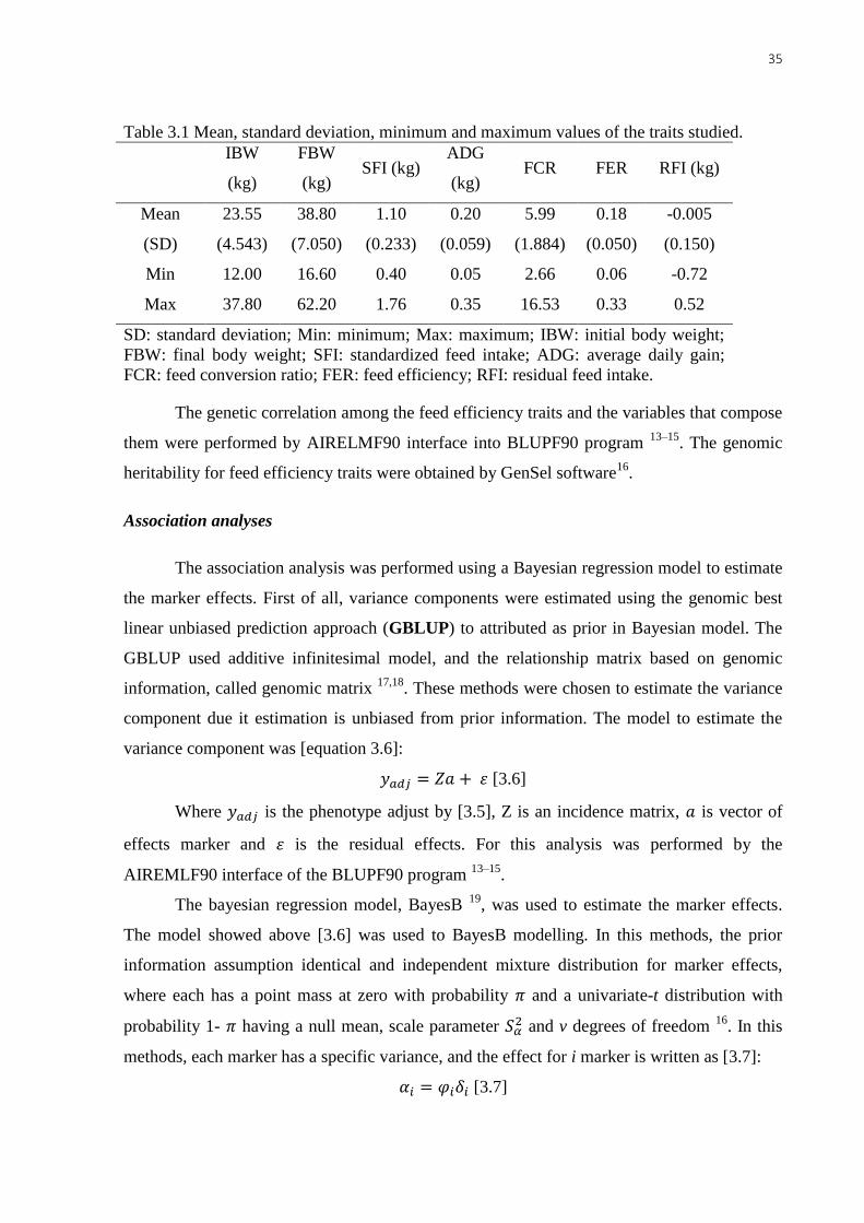
35

Table 3.1 Mean, standard deviation, minimum and maximum values of the traits studied.

IBW

(kg)

FBW

(kg) SFI (kg)

ADG

(kg) FCR FER RFI (kg)

Mean

(SD)

23.55

(4.543)

38.80

(7.050)

1.10

(0.233)

0.20

(0.059)

5.99

(1.884)

0.18

(0.050)

-0.005

(0.150)

Min 12.00 16.60 0.40 0.05 2.66 0.06 -0.72

Max 37.80 62.20 1.76 0.35 16.53 0.33 0.52

SD: standard deviation; Min: minimum; Max: maximum; IBW: initial body weight;

FBW: final body weight; SFI: standardized feed intake; ADG: average daily gain;

FCR: feed conversion ratio; FER: feed efficiency; RFI: residual feed intake.

The genetic correlation among the feed efficiency traits and the variables that compose

them were performed by AIRELMF90 interface into BLUPF90 program 13–15

. The genomic

heritability for feed efficiency traits were obtained by GenSel software16

.

Association analyses

The association analysis was performed using a Bayesian regression model to estimate

the marker effects. First of all, variance components were estimated using the genomic best

linear unbiased prediction approach (GBLUP) to attributed as prior in Bayesian model. The

GBLUP used additive infinitesimal model, and the relationship matrix based on genomic

information, called genomic matrix 17,18

. These methods were chosen to estimate the variance

component due it estimation is unbiased from prior information. The model to estimate the

variance component was [equation 3.6]:

𝑦𝑎𝑑𝑗 = 𝑍𝑎 + 휀 [3.6]

Where 𝑦𝑎𝑑𝑗 is the phenotype adjust by [3.5], Z is an incidence matrix, 𝑎 is vector of

effects marker and 휀 is the residual effects. For this analysis was performed by the

AIREMLF90 interface of the BLUPF90 program 13–15

.

The bayesian regression model, BayesB 19

, was used to estimate the marker effects.

The model showed above [3.6] was used to BayesB modelling. In this methods, the prior

information assumption identical and independent mixture distribution for marker effects,

where each has a point mass at zero with probability 𝜋 and a univariate-t distribution with

probability 1- 𝜋 having a null mean, scale parameter 𝑆𝛼2 and v degrees of freedom

16. In this

methods, each marker has a specific variance, and the effect for i marker is written as [3.7]:

𝛼𝑖 = 𝜑𝑖𝛿𝑖 [3.7]

36

Where 𝜑𝑖 has a normal distribution with null mean and locus-specific variance 𝜎𝑖2,

which in turn has a scale inverse chi-square prior with scale parameter 𝑆𝛼2 and v degrees of

freedom. In this methods, the 𝜋 is known and for this study were represent by 0.99. Thus, we

assume that percentage part of the markers is associated with phenotype. The genome-wide

association was performance by the GenSel software 16

.

Finally, the marker was classified as significantly association with the phenotype

based on bayes factor (BF) parameter. The BF was written as:

𝐵𝐹𝑖 =(

𝜌𝑖1−𝜌𝑖

)

(1−𝜋

𝜋) [3.8]

Where 𝜌𝑖 is a posterior frequency of a marker to be in the model for each i SNP. The

classification for a marker as defined as when 𝐵𝐹𝑖 is higher than three, can be considered as

suggestive linkage between marker and causal mutation. The BF range (20 to 150) indicates

linkage between marker and causal mutation. Finally, BF higher 150 is a very strong evidence

of linkage 20

.

The finding of candidate genes was performance by ENSEMBL website platform

(http://www.ensembl.org/). The variant consequence of significant SNPs by BF was found

into variant effect predictor platform of ENSEMBL website (VEP -

http://www.ensembl.org/info/docs/tools/vep/index.html). Finally, the candidates genes was

characterized by gene ontology (GO) terms21

.

3.3 Results

Phenotyping and genotyping data

The average for FCR, FER and RFI were equal to 5.990, 0.180 and -0.005 kg,

respectively. Remarkably, RFI presented average close to zero due to it is residual parameter

consequently, will have a normal distribution with mean zero.

For association and complementary analyses remained 43,779 SNPs and 386 animals.

Descriptive analysis for data quality control was: call rate lower than 0.90 excluded 3,463

SNPs; MAF lower than 0.05, 5,942 SNPs were excluded; and p-value lower than 0.1 for

Hardy-Weinberg Equilibrium Chi-square test, 1,057 SNPs were excluded. One sample with

call rate lower than 0.9 was also removed.

37

Genetic correlations and heritability

The genomic heritability for RFI, FER and FCR were 0.75, 0.26 and 0.30,

respectively. The genomic heritability estimatives were analyzed for convergence test by

Heidelberger & Welch, which all passed for this test. The genetic correlations among feed

efficiency traits and feed intake, gain daily weight and life body weight are showed in off-

diagonal Table 3.2.

Table 3.2 Genetic correlations of feed efficiency traits and variables that compose them.

Traits RFI FCR FER ADG SFI

RFI

FCR -0.549

FER 0.232 0.990

ADG -0.037 0.989 0.998

SFI 0.021 0.997 0.996 -0.999

metabolicMIDWT -0.493 0.999 0.998 0.972 0.999

RFI: Residual feed intake; FCR: Feed conversion ratio; FER: feed efficiency ratio; ADG:

average daily gain; SFI: standardized feed intake; metabolicMIDWT: metabolic mid-point

weight.

Genome-wide association

After quality control, 43,779 SNPs and 386 animals remained in this study, which

were used in association analysis. Four SNPs were strongly associate with the efficiency

metrics (BF>20), and one 126 SNPs were classified as suggestive association (BF>3; Table

3.3) according to Bayes factor estimatives. The Figure 3.1 shows the representative bayes

factor (BF) of each SNP per chromosome for the three feed efficiency traits: RFI, FER and

FCR.

Comparing the efficiency traits, a higher number of significative SNP were observed

for RFI. Moreover, no associated SNP to RFI was common with other traits. We initially

expected this, because the RFI is independent of body weight and weight gain 11,12

,

consequently, its theory is to selected efficient animals without select animals with high

weight and rate gain, different of FER and FCR.

38

Table 3.3 Number of SNP classify as suggestive (BF > 3) or strongly (BF > 20) association

for residual feed intake, feed efficiency and feed conversion ratio.

Category RFI FER FCR Coincident SNPs

RFI:FER RFI:FCR FE:FCR

Suggestive 104 4 17 0 0 1

Strongly 4 0 0 0 0 0

RFI: residual feed intake; FER: feed efficiency ratio; FCR: feed conversion ratio.

Between FER and FCR was possibly verify one commonly SNP. The SNP

OAR11_8626515.1, located on OAR11, and it being inside of ENSOARG00000011009 gene

with uncharacterized protein. Our initially hypothesis is that at least one SNP will be similar

between this traits, because they are a function of the same variable, being only inversely

proportional.

The Table 3.4 presents the SNPs that are located inside of gene probably associated

with the phenotype (direct or indirect), chromosome, position, SNP effect and bayes factor.

Other SNPs were presented in Supplementary tables 3.1.

A total of 80 SNPs (55 %), which were significant, located into intergenic variant; 35

SNPs (31 %) located into intron variant; 9 SNPs (6 %) located into non-coding transcript

variant; 6 SNPs (4 %) located into downstream gene variant; 3 SNPs (2 %) located into

upstream gene variant; and 1 SNP (1 %) located into splice region variant (Figure 3.2).

3.4 Discussion

The understood of genetic mechanisms underlying traits could be important for

identification of candidate genetic variances in genomic selection studies, candidate genes,

and consequently, knowledge about the biological process that interferes into trait responses.

All these findings could help to drive new insights to optimize the animal production (animal

breeding approach, animal management, and nutrition) 8.

Genetic correlations and heritability

The RFI heritability estimated in this study was relatively higher than other. In lambs

without genomic information was found the heritability for RFI equal to 0.2622

. Verifying the

heritability without genomic information in another ruminant specie, bovine, the heritability

was 0.16 23

. In pigs, also without genomic information, was found RFI heritabilities values

39

ranging from 0.34 to 0.40. For FER heritability, the value was similar with the estimation

without genomic information in lamb (0.26) 22

, in bovine (0.26) 23

and in pig (0.30- 0.32) 24

.

It is understood that the genomic heritability might overestimated compared with

heritability based on pedigree information. However, the FER heritability was similar to other

studies. Moreover, Bolormaa et al. (2013) founded heritability for RFI using genomic

information equal to 0.36 25

, established by the overestimation of RFI heritability.

Figure 3.1 Manhattan plot of bayes factor of each SNP per chromosome for three traits of

animal efficiency: residual feed intake (RFI), feed efficiency ratio (FER) and feed conversion

ratio (FCR).

40

Table 3.4 SNP associated, respectively gene, chromosome, position, SNP effect and bayes factor.

Trait SNP Ensemble (gene) Gene Chr:Position Effect %𝜎𝑔2 Allele BF

RFI rs417277672 ENSOARG00000020653 MCF2L2 1:202056238 0.00146 0.0002 [T/G] 4.79534

RFI rs416195886 ENSOARG00000007440 GRIN3A 2:21252248 -0.0014 0.00018 [A/G] 4.27561

RFI rs425114550 ENSOARG00000004714 NRF1 4:93569119 -0.0039 0.00042 [T/C] 9.92287

RFI rs424957575 ENSOARG00000000875 TPM4 5:6669927 0.00109 0.00013 [A/G] 3.0829

RFI rs409680528 ENSOARG00000000337 MAP3K5 8:61642640 0.00283 0.00035 [A/G] 8.21248

RFI rs411939214 ENSOARG00000001541 PEX3 8:67841404 -0.002 0.0002 [T/C] 4.53483

RFI rs420010466 ENSOARG00000009854 EXT1 9:58992455 -0.0012 0.00015 [T/C] 3.27273

RFI rs413906063 ENSOARG00000011562 YBX2 11:26623188 -0.0027 0.00032 [T/G] 7.47451

RFI rs414722940 ENSOARG00000015595 BPTF 11:48432323 -0.0015 0.0002 [A/G] 4.57815

RFI rs398294146 ENSOARG00000004714 NUMA1 15:49881907 0.01061 0.00123 [T/G] 35.4013

FC rs405741086 ENSOARG00000015353 FAM160B1 22:34265670 -0.0047 0.0005 [T/C] 3.38908

Effect: additive effect of marker into phenotype; %𝜎𝑔2 additive genetic variance explained by marker; Allele: nucleotide

base variation for marker; BF: bayes factor.

41

In lamb, the genetic correlation using only pedigree information between FER and FI

was high, 0.79, and RFI with FI was 0.7722

. The genetic correlation between FER and RFI

was low (0.23)22

. In bovine, the correlation between RFI and FER, SFI, ADG, and

metabolicMIDWT were 0.70, 0.64, 0.09 and 0.93, respectively23

. Our correlations contrasting

with other studies, observing underestimation of our values.

Genome-wide association

Despite of differences in the estimation of efficient animals, the results did not show

similar genetic architecture between the traits (number of associated SNPs). Probably, the RFI

presents a large number of associated SNPs due to higher heritability (0.75) than other two

traits studied herein. Significant SNPs associated with RFI were similarly distributed on the

genome, which on chromosomes 14, 18, 21, 24 and 25 did not appear any SNP. The

chromosomes with a higher density of association and similarly SNPs between traits were on

OAR1 to OAR5, OAR7, OAR11:OAR13, OAR15:OAR17, OAR20, OAR 22, OAR23 and

OAR27.

As an introduction of biological mechanisms that might control RFI variation,

Richardson and Herd (2004) 26

estimated many physiological mechanisms that contribute,

such as protein turnover, tissue metabolism and stress, which was responsible by 37%;

activity (10%); digestibility (10%); heat increment of fermentation (9%); body composition

(5%); and feeding patterns (2%).

On chromosome one, OAR1, eleven associated SNPs were present, which those three

being inside or behind a known gene. The SNP rs417277672 were found at 202.06 mega base

pairs (Mb) positions (intron variant), with effect and BF equal to 0.0015 and 4.80,

respectively. The MCF2L2 (MCF.2 cell line derived transforming sequence-like 2) gene,

located at 201.87 - 202.21 Mb region, might be an interesting candidate gene. This gene was

positively correlated with insulin secretion and it was more expressed in the

nondiabetic/normoglycemic person27

. The normal insulin secretion wished for the efficiency

use of glucose, mainly responsible by all activities of body. We were not able to find any

study correlating feed efficiency and insulin secretion. However, the study with aim to

understand the relationship between the insulin concentration and RFI, found a positive

genetic relationship among both 26

. Moreover, it was observed that the insulin concentration

tended to be higher in the higher-RFI animals 26

. The higher insulin concentration was related

mainly with high feed intake and high feeding times, which have negative correlation with

RFI 26

.

42

The SNP rs416195886 located on chromosome 2 at 21.25 Mb position (intron variant),

with effect and BF equal to -0.0014 and 4.28. This marker being inside of gene GRIN3A

[glutamate ionotropic receptor N-methyl-D-aspartate (NMDA) type subunit 3A], were

comprising the 21.25 - 21.46 Mb position. The NMDA receptor effects on neuronal activity.

The NRF-2 and NRF-1 mediated this activity, as well as, the energy metabolism activity. The

transcription levels of GRIN3A increases when the NRF-2 decreased. On the other hand, the

levels of GRIN3A decreases significantly on the situation with over-expression of NRF-2 28

.

Additionally, the SNP rs425114550 (OAR4 at 93.56 MB) appear such as significant

on our analyses, being inside of NRF-1 (nuclear respiratory factor 1) gene delimiting of 93.54

to 93.62 Mb. This gene is an transcription factor, which participate in mitochondrial processes

of biosynthesis, more specifically on electron transportation chain 29

.

The mitochondria is responsible for production of more than 90% energy used by

cells, as well as, the energy dissipated (lost energy) 29

, which represents 25% of total basal

metabolic rate of animal 30,31

. More efficiency animals (negative RFI) presents lower rates of

electron lost than less efficiency animals (positive RFI), and this electron was dissipated on

electron transportation chain 32

. Consequently, the higher levels of electron lost, will provide

an environment with heat release, more reactive oxygen and less ATP, resulting in more

required of feeding 33

.

On chromosome 5, the SNP rs424957575, located at 6.67 Mb, being beside from

TPM4 gene (Tropomyosin 4- 6.65-6.67 Mb) of 205-distance basis. On animals group of high-

feed efficiency were characterized such as downregulated genes related to major

histocompatibility complex cell recognition, stress-related heat shock protein, and most

important for the region measure here (OAR5 at 6.67 Mb), several genes associated with

muscle fibers or cytoskeletal architecture (e.g. tropomyosin) 34

. The specific allele copy of the

SNP nearly from TPM4 results a negative impact on phenotype.

Another important SNP such as rs425114550 (associated to NRF-1) is the

rs409680528, located on chromosome 8 at 61.64 Mb position. This SNP being inside of

MAP3K5 gene (Mitogen-Activated Protein Kinase 5) 61.57-61.80 Mb. Studies based on

MAP3K5 related this gene to residual feed intake using molecular cloning, characterization,

tissue expression pattern, and copy number variations were did, and found useful information

regarding the influence of MAP3K5 on RFI in pigs 35

. The relative copy number of MAP3K5

was higher in low RFI Duroc pigs than in high 35

.

Moreover, in pig, this gene was cited on genome-wide association study for RFI, and

concluded that this gene can be an interesting candidate 36

. The effect of MAP3K5 (or in

43

generally, MAPK) on controlling feed efficiency traits may be mediated by variety of

pathways such as hormones and growth factors that act through receptor tyrosine kinases,

cytokine receptors to vasoactive peptides acting through G protein-coupled and seven-

transmembrane receptors 36

. Among these pathways, was observed a positive correlation

between insulin growth factor 1 (IGF1) (growth factor) concentration and RFI 26

.

On OAR9, the candidate gene is EXT1 (exostosin 1 – from 58.994 to 59.42 Mb)

because the rs420010466 SNP beside it (58.992 Mb). This gene was found in a quantitative

trait loci (QTL) region to carcass weight (CWT) and eye muscle area in bovine (EMA). In

this examples, , this gene was more highly expressed in muscle samples from animals with

increasing CWT and EMA 37

.

On OAR11, two SNPs were associated with two candidate genes relating to

reproductive traits. The first is the rs413906063 SNP located in 26.62 Mb with effect and BF

equal to -0.0027 and 7.47, respectively. This SNP is located inside of YBX2 gene (Y-box

binding protein 2; from 26.62 to 26.62 Mb). This gene is an upstream regulator of protamine

expression, implicated in male infertility 38

. Supporting this idea, a recent study shows that the

percentage of azoospermia in humans change as the YBX2 genotype change 39

. Besides, in

the same chromosome, the gene BPTF (Bromodomain PHD finger transcription factor; from

48.38 to 48.47 Mb) is responsible to regulate and signaling pathways of embryos and

embryonic stem cells in early mouse 40

. In general, the reproduction and feed efficiency to

deposition of meat or milk has negative correlation (Reference). It held due the energy

directly to reproduction, needing more consumption to attend this physiology and the

production.

On OAR5, the rs398294146 SNP was classified as strong association with phenotype.

This SNP presented effect and BF equal to 0.011 and 35.40, respectively, and located in 49.88

where being inside of NUMA1 gene (nuclear mitotic apparatus protein 1; from 49.85 to 49.88

Mb). This gene was found in a group of differentially methylated gene in small intestine of

piglet were directly connected with ubiquitin C to form a network concerned with cancer, cell

to cell signaling and interaction and cellular growth and proliferation 41

. In addition, this gene

is thought to be associated with the formation of villi of newborn, and villi plays an important

role in absorption of nutrients by expanding the surface of small intestine 41

. The absorption

able of nutrients could be related with digestibility able, which are negatively correlated with

RFI (-0.44) 37

.

On OAR22 the rs405741086 SNP (34.27 Mb) being inside of FAM160B1 gene

(family with sequence similarity 160 member B1; from 34.26 to 34.29 Mb). The FAM160B1

44

was downregulated in fat-fed protein kinase C-deficient in mice 42

. On the other hand, this

gene was associated with non-obstructive azoospermia (NOA), whereas patients with NOA

the expression of FAM160B1 is lower than patients without NOA 43

.

In conclusion, many SNPs inside candidate genes were briefly presented in this study.

The main pathways that they involves were mitochondrial biosynthesis, insulin secretion,

growth factor, digestibility and reproduction. Moreover, no SNP coincident was observed

between RFI and FER or FCR, as except. We initially hypothesis was found few or many

SNPs coincident between FER and FCR, however, we found only one.

References

1. Westhuizen, R. R. Van Der, Westhuizen, J. Van Der & Schoeman, S. J. Genetic variance

components for residual feed intake and feed conversion ratio and their correlations with other

production traits in beef bulls. S. Afr. J. Anim. Sci. 34, 257–264 (2004).

2. Crutzen, P. J., Aselmann, I. & Seiler, W. Methane production by domestic animals, wild

ruminants, other herbivorous fauna, and humans. Tellus B 38 B, 271–284 (1986).

3. Blaxter, K. L. & Clapperton, J. L. Prediction of the amount of methane produced by ruminants.

Br. J. Nutr. 19, 511–522 (1965).

4. Pelchen, A. & Peters, K. J. Methane emissions from sheep. Small Rumin. Res. 27, 137–150

(1998).

5. Hegarty, R. S., Goopy, J. P., Herd, R. M. & McCorkell, B. Cattle selected for lower residual

feed intake have reduced daily methane production. J. Anim. Sci. 85, 1479–1486 (2007).

6. Koch, R. M., Swiger, L. A., Chambers, D. & Gregory, K. E. Efficiency of feed use in beef

cattle. J. Anim. Sci. 22.2, 486–494 (1963).

7. Arthur, P. F. et al. Genetic and phenotypic variance and covariance components for feed

intake, feed efficiency, and other postweaning traits in Angus cattle. J. Anim. Sci. 79, 2805–

2811 (2001).

8. Kadarmideen, H. N., Von Rohr, P. & Janss, L. L. G. From genetical genomics to systems

genetics: Potential applications in quantitative genomics and animal breeding. Mamm. Genome

17, 548–564 (2006).

9. Do, D. N., Strathe, A. B., Ostersen, T., Pant, S. D. & Kadarmideen, H. N. Genome-wide

association and pathway analysis of feed efficiency in pigs reveal candidate genes and

pathways for residual feed intake. Front. Genet. 5, 1–10 (2014).

10. Santana, M. H. et al. Genome-wide association analysis of feed intake and residual feed intake

in Nellore cattle. BMC Genet. 15, 21 (2014).

11. Archer, J. a, Arthur, P. F., Herd, R. M., Parnell, P. F. & Pitchford, W. S. Optimum postweaning

test for measurement of growth rate , feed intake , and feed efficiency in British breed cattle. J.

Anim. Sci. 75, 2024–2032 (1997).

12. Arthur, P. F., Renand, G. & Krauss, D. Genetic and phenotypic relationships among different

measures of growth and feed efficiency in young Charolais bulls. Livest. Prod. Sci. 68, 131–

139 (2001).

13. Legarra, a, Aguilar, I. & Misztal, I. A relationship matrix including full pedigree and genomic

information. J. Dairy Sci. 92, 4656–4663 (2009).

14. Misztal, I., Legarra, A. & Aguilar, I. Computing procedures for genetic evaluation including

phenotypic, full pedigree, and genomic information. J. Dairy Sci. 92, 4648–4655 (2009).

45

15. Aguilar, I. et al. Hot topic: a unified approach to utilize phenotypic, full pedigree, and genomic

information for genetic evaluation of Holstein final score. J. Dairy Sci. 93, 743–52 (2010).

16. Fernando, R. L. & Garrick, D. J. in Genome-Wide Association Studies and Genomic Prediction

1, 1–565 (2013).

17. VanRaden, P. M. et al. Invited review: reliability of genomic predictions for North American

Holstein bulls. J. Dairy Sci. 92, 16–24 (2009).

18. de los Campos, G., Hickey, J. M., Pong-Wong, R., Daetwyler, H. D. & Calus, M. P. L. Whole-

genome regression and prediction methods applied to plant and animal breeding. Genetics 193,

327–345 (2013).

19. Meuwissen, T. H. E., Hayes, B. J. & Goddard, M. E. Prediction of total genetic value using

genome-wide dense marker maps. Genetics 157, 1819–1829 (2001).

20. Vidal, O. et al. Identification of carcass and meat quality quantitative trait loci in a Landrace

pig population selected for growth and leanness. Am. Soc. Anim. Sci. 83, 293–300 (2005).

21. Ashburner, M. et al. Gene Ontology: tool for the unification of biology. Nat. Genet. 25, 25–29

(2000).

22. Snowder, G. D. & Van Vleck, L. D. Estimates of genetic parameters and selection strategies to

improve the economic efficiency of postweaning growth in lambs. Am. Soc. Anim. Sci. 81,

2704–2713 (2003).

23. Herd, R. M. & Bishop, S. C. Genetic variation in residual feed intake and its association with

other production traits in British Hereford cattle. Livest. Prod. Sci. 63, 111–119 (2000).

24. Do, D. N., Strathe, A. B., Jensen, J., Mark, T. & Kadarmideen, H. N. Genetic parameters for

different measures of feed efficiency and related traits in boars of three pig breeds. J. Anim. Sci.

91, 4069–4079 (2013).

25. Bolormaa, S. et al. Accuracy of prediction of genomic breeding values for residual feed intake

and carcass and meat quality traits in Bos taurus, Bos indicus, and composite beef cattle. J.

Anim. Sci. 91, 3088–3104 (2013).

26. Richardson, E. C., Herd, R. M., Archer, J. a. & Arthur, P. F. Metabolic differences in Angus

steers divergently selected for residual feed intake. Aust. J. Exp. Agric. 44, 441 (2004).

27. Taneera, J. et al. Identification of novel genes for glucose metabolism based upon expression

pattern in human islets and effect on insulin secretion and glycemia. Hum. Mol. Genet. 24,

1945–1955 (2014).

28. Priya, A., Johar, K. & Wong-Riley, M. T. T. Nuclear respiratory factor 2 regulates the

expression of the same NMDA receptor subunit genes as NRF-1: Both factors act by a

concurrent and parallel mechanism to couple energy metabolism and synaptic transmission.

Biochim. Biophys. Acta - Mol. Cell Res. 1833, 48–58 (2013).

29. Bottje, W. G. & Carstens, G. E. Variation in Metabolism: Biological Efficiency of Energy

Production and Utilization That Affects Feed Efficiency. Feed Effic. Beef Ind. 251–273 (2012).

doi:10.1002/9781118392331.ch15

30. Rolfe, D. F. S. & Brand, M. D. The physiological significance of mitochondrial proton leak in

animal cells and tissues. Biosci. Rep. 17, 9–16 (1997).

31. Rolfe, D. F. & Brand, M. D. Contribution of mitochondrial proton leak to skeletal muscle

respiration and to standard metabolic rate. Am. J. Physiol. 271, C1380–C1389 (1996).

32. Bottje, W. et al. Association of mitochondrial function with feed efficiency within a single

genetic line of male broilers. Poult. Sci. 81, 546–555 (2002).

33. Bottje, W., Pumford, N. R., Ojano-Dirain, C., Iqbal, M. & Lassiter, K. Feed efficiency and

mitochondrial function. Poult Sci 85, 8–14 (2006).

34. Bottje, W. & Kong, B.-W. CELL BIOLOGY SYMPOSIUM: Feed effi ciency: Mitochondrial

function to global gene expression 1,2. J. Anim. Sci 91, 1582–1593 (2013).

46

35. Pu, L. et al. Porcine MAP3K5 analysis: Molecular cloning, characterization, tissue expression

pattern, and copy number variations associated with residual feed intake. Genet. Mol. Res. 15,

1–13 (2016).

36. Do, D. N. et al. Genome-wide association and systems genetic analyses of residual feed intake,

daily feed consumption, backfat and weight gain in pigs. BMC Genet. 15, 27 (2014).

37. Lee, S. H. et al. QTL and gene expression analyses identify genes affecting carcass weight and

marbling on BTA14 in Hanwoo (Korean Cattle). Mamm. Genome 22, 589–601 (2011).

38. Hammoud, S., Emery, B. R., Dunn, D., Weiss, R. B. & Carrell, D. T. Sequence alterations in

the YBX2 gene are associated with male factor infertility. Fertil. Steril. 91, 1090–1095 (2009).

39. Chihara, M. et al. Association of NR3C1/Glucocorticoid Receptor gene SNP with azoospermia

in Japanese men. J. Obstet. Gynaecol. Res. 42, 59–66 (2016).

40. Landry, J. et al. Essential role of chromatin remodeling protein bptf in early mouse embryos

and embryonic stem cells. PLoS Genet. 4, (2008).

41. Kwak, W. et al. Genome-wide DNA methylation profiles of small intestine and liver in fast-

growing and slow-growing weaning piglets. Asian-Australasian J. Anim. Sci. 27, 1532–1539

(2014).

42. Liao, B. M. et al. Proteomic analysis of livers from fat-fed mice deficient in either PKCδ or

PKCε identifies Htatip2 as a regulator of lipid metabolism. Proteomics 14, 2578–2587 (2014).

43. Zhang, Y. et al. A susceptibility locus rs7099208 is associated with non-obstructive

azoospermia via reduction in the expression of FAM160B1. J. Biomed. Res. 29, 491–500

(2015).

47

4. GENOMIC SELECTION FOR RESIDUAL FEED INTAKE USING A

SMALL OVINE POPULATION

Amanda Botelho Alvarenga1, Gregori Alberto Rovadoscki

1, Juliana Petrini

1, Gota

Morota², Aline Silva Mello Cesar¹, Luiz Lehmann Coutinho1, Matthew L. Spangler², Eula

Regina Carrara¹, Gleidson Giordano Pinto de Carvalho3, Luís Fernando Batista Pinto

3 and

Gerson Barreto Mourão1*

1 Department of Animal Science, University of São Paulo (USP) / Luiz de Queiroz College of

Agriculture (ESALQ), Piracicaba, SP, Brazil

2 Department of Animal Science, University of Nebraska, Lincoln, NE, USA

3 Department of Animal Science, Federal University of Bahia (UFBA), Salvador, BA, Brazil

ABSTRACT

The selection on genetic values predicted from markers could substantially increase

the rate of genetic gain in animals and plants, especially if combined with reproductive

techniques to shorten the generation interval. However, the accuracy of genomic selection

(GS) might vary depending on several factors, such as the heritability of trait, linkage

disequilibrium in the population, size of the training population and relationship between

animals in the training and target populations. Consequently, it is important to evaluate the

prediction accuracy of genomic estimated breeding value (GEBV) to ensure desired response

to selection and determine the potential cost/benefit of implementing GS. In this study, we

proposed to evaluate the accuracy of GEBV in ovine, characterized by Santa Inês breed, for

one of the most economically relevant traits in animal production, feed efficiency represented

by residual feed intake (RFI). This is the first research in ovine using genomic information

for efficiency traits. We used a genotyping data comprising 54,241 single nucleotide

polymorphism panel (SNP) for 387 animals (Illumina High-Density Ovine SNP BeadChip®).

We chose two Bayesian regression models to estimate marker effects (BayesA and BayesB).

For BayesB models we compared three different 𝜋 values (0.99 and 0.9912). Accuracies were

characterized by Pearson’ correlation between the GEBV and adjusted phenotype, and it was

estimated by two-fold cross-validation. Of the other models compared accuracies for GEBV

were similar with averages being 0.036 (BayesA), 0.034 (BayesB, 𝜋=0.99) and 0.033

(BayesB, 𝜋=0.9912). Negative accuracies were estimated in five training-validation groups

for all methods. We contend that the poor prediction accuracies were observed due to: low

average linkage disequilibrium between adjacent markers in ovine (r²=0.16), low or null

average relationship between animals (0.0011), and the small training population used (193

animals).

Keywords: BayesA, BayesB, Bayesian model regression, Cross-validation, Feed efficiency,

Genomic selection, Genomic relationship, Linkage disequilibrium, Ovine.

4.1 Introduction

48

The ability of animals to convert the feed consumed into final products impacts the

costs of production due to improved feed utilization, and also have an environmental impact

because of reduced methane emission and decreased resources (e.g., land) needed for

production 1,2

. Many traits measure the efficiency of animals in converting feed into products,

such as the ratio between weight gain and feed intake, the ratio between feed intake and

weight gain and residual feed intake (RFI). The ratio between weight gain and feed intake

and the ratio between feed intake and weight gain can result in over estimation of efficiency

because they do not consider the feed required for maintenance 3. Koch et al. (1963)

3

proposed RFI, which is feed intake adjusted for differences in feed consumption for average

daily weight gain (ADG) and metabolic mid-point weight (metabolicMIDWT). RFI is the

difference between the feed consumption and the expected feed consumption.

Techniques that maximize feed efficiency traits are important. Changes of feed

efficiency through genetic selection is possible due to the medium to high heritability

associated with these traits3. However, the use of genetic selection for feed efficiency traits is

limited because they are expensive and difficult to measure, mainly in extensive production

systems. Genomic information can solve this problem because it permits the selection of

animals based on the entire genome through an approach called genomic selection (GS).

GS is the selection of individuals based on the genome-wide information of hundreds

or thousands of markers, such as single nucleotide polymorphisms (SNP). In bovine and

swine for example, many studies were developed and positive results were obtained. For Bos

taurus and Bos indicus breeds, the average accuracy found (standard deviation) for the

genomic estimated breeding value (GEBV) across seven breeds was 0.36 (0.14)4 with a

moderate to high accuracy for RFI.

However, no study involving genomic selection for feed efficiency traits in ovine has

been previously published. Since the present study is a pioneer research with genomic

selection in Ovis aries for feed efficiency, the number of animals used is still small. The use of

small genotyped and phenotyped population configures a challenge in getting high accuracies,

not only in this study, but also for other that have limited access of data. The ovine production

is a promising livestock, mainly in Brazil, due to increase consumption of meat sheep during

years. Besides, the Brazil does not supply the meat sheep demand within country and the

country does not have participation on exportation of meat, such as bovine, pig and chicken.

Techniques that may maximize the meat production by herd is interesting to country and

world economy, as well as to environmental impacts. Therefore, the aim of this study was to

evaluate the accuracy of GEBV for RFI in an ovine population, characterized by Brazilian

49

Santa Inês breed. A resistant breed, adapting to different conditions, as well as nice

reproductive traits performance, characterizes the Santa Inês sheep.

4.2 Methods

Phenotype estimation and population structure

All phenotypic data used in this study are from 387 Santa Inês sheep. All animals were

uncastrated, vaccinated, and dewormed, and recorded at the Experimental Farm of São

Gonçalo dos Campos, city of São Gonçalo dos Campos, Bahia, Brazil, which is associated

with the Federal University of Bahia (UFBA), during a period of two years (2016 to 2017).

Sheep were given feed and water ad libitum. These animals were maintained in individual

stalls during 54 to 92 days, conducted at four different periods and with a mean age (standard

deviation) of 120 (60) days. The animals received diets ranging from 11 to 16% crude protein

among contemporary groups, all of them formulated according to the NRC (2007).

Contemporary groups (n = 27, composed of 9 to 18 animals) were formed by animals from

the same herd commercial and period of confinement.

Feed intake (FI) was measured manually as the difference between the feed provided

and leftovers. Feed intake was converted to dry matter intake (DMI). The body weight gain

(BWG) was measured as the deviation of final body weight (FBW) from the initial body

weight (IBW), both with 16 hours of fasting. The mean (standard deviation) for IBW and

FBW of 23.5 (4.54) and 38.9 (5.05) kilograms (kg), respectively.

Both variables, DMI and WBG, were divided by days in confinement to obtain the

parameters per day, which were used to estimate efficiency metrics, resulting in standardized

feed intake (SFI) and average daily gain (ADG).

Residual feed intake (RFI) is an efficiency indicator metric, which accounts for body

weight in its estimation [equation 4.1]. Consequently, improvement could be made in RFI

without affecting body size and growth rate 5,6

.

𝑅𝐹𝐼𝑘𝑔 = 𝑆𝐹𝐼(𝑘𝑔) − 𝐸𝐹𝐼(𝑘𝑔) [4.1] 3

Where the EFI is an expected feed intake. To calculate the EFI, ADG and metabolic mid-

point weight (metabolicMIDWT- equation 4.2) were used to model daily SFI 5,6

. A model was

fitted using the GLM procedure of the SAS Institute, Inc. (1996). The resulting equations

were [equation 4.3]:

metabolicMIDWT= ((𝐼𝐵𝑊 + 𝐹𝐵𝑊)

2⁄ )0.75 [4.2]

50

𝐸𝐹𝐼(𝑘𝑔) = −0.15187 + 0.97868 ∗ 𝐴𝐷𝐺 + 0.08286 ∗ 𝑚𝑒𝑡𝑎𝑏𝑜𝑙𝑖𝑐𝑀𝐼𝐷𝑊𝑇 [4.3]

The phenotypes used in genomic analysis were previously adjusted for the fixed effect

of contemporary group [equation 4.4].

𝑦𝑖𝑗 = 𝜇𝑗 + 𝑣𝑖𝑗 + 휀𝑖𝑗 [4.4]

Where 𝑦𝑖 is the phenotype of animal i of contemporaneous group j; 𝜇 is the phenotype

mean in contemporary group j; 𝑣𝑖𝑗 is the contemporaneous group j assigned to animal i; and

휀𝑖𝑗 is the residual effect for animal i, ~ N(0,𝜎𝑒2). The adjusted phenotype was estimated by the

sum of the actual phenotype and the residual estimated from [equation 4.4].

The genomic relationship between animals was estimated by the G7 matrix constructed

by using the PREGSF90 software of the BLUPF90 package 8–10

. Inbreeding coefficient (F)

was also calculated as a function of the expected and observed homozygote difference by

using PLINK software 11

. This is given by:

𝐹𝑖 =(𝑂𝑖−𝐸𝑖)

(𝐿𝑖−𝐸𝑖) [4.5]

Where 𝑂𝑖 is the number of homozygous loci observed in the ith

animal, 𝐸𝑖 is the

expected number of homozygous loci and 𝐿𝑖 is the number of genotyped autosomal loci 11

.

Genotyping and quality control

DNA was extracted from samples of the Longissimus dorsi muscle tissue collected

from the left hemi-carcass and stored in 2.0 milliliter (ml) Eppendorf tubes. DNA extraction

was performed according to protocols using lysis buffer and RNase. A high-density panel of

SNP (Illumina High-Density Ovine SNPs BeadChip®) comprising 54,241 SNP was used for

genotyping. Chromosomal coordinates for each SNP were obtained by ovine genome

sequence assembly, Oar_v3.1. Quality control (QC) of the genomic data was performed by

using the PREGSF90 interface of the BLUPF90 program 8–10

. SNPs with a call rate lower

than 0.90 (n= 3,463), minor allele frequency (MAF) lower than 0.05 (n=5,942) and p-value

lower than 0.1 for the Hardy-Weinberg Equilibrium Chi-square test (n=1,057) were excluded,

remaining 43,779 SNPs. One sample with call rate lower than 0.9 was also removed.

Association analysis

The association analysis used a Bayesian regression model to estimate the marker

effects. First of all, variance components was estimated using the genomic best linear

unbiased prediction approach (GBLUP), which were attributed as prior values in the

Bayesian model. The GBLUP used additive infinitesimal model, and the relationship matrix

51

based on genomic information, called genomic relationship matrix 12,13

. These methods were

chosen to estimate the variance components because its estimation is more independent from

the prior information. The model used to estimate the variance components was [equation

4.6]:

𝑦𝑎𝑑𝑗 = 𝑍𝑎 + 𝑒 [4.6]

Where 𝑦𝑎𝑑𝑗 is the phenotype adjust by [4.4] (n x 1); Z is an incidence matrix of

random effects additive genetic; 𝑎 is the vector of genetic additive effects ~ 𝑁(0, 𝐺𝜎𝑎2); where

G is a genomic relationship matrix and 𝜎𝑎2 additive genetic variance; and 휀 is vector of the

residual effects, with normal distribution 𝑒|𝜎𝑒2 ~𝑁(𝑒|0, 𝐼𝜎𝑒

2). This analysis was performed by

the AIREMLF90 interface of the BLUPF90 program 8–10

.

The Bayesian regression model was used to estimate the marker effects. The Bayesian

method is characterized by a combination of data (likelihood) and additional information

(prior). We used two methods initially proposed by Meuwissen et al. (2001)14

that assume

different marker effect variance. In the other words, the BayesA and BayesB have a similar

feature characterized by a marker specific variance..

BayesA method uses the prior knowledge that many SNPs have small individual

effects on the trait and only a few SNPs have moderate to large effect, consequently, all

markers have an effect on phenotype (𝜋 equal to zero) 14

. The marker genetic variance follows

a scaled inverted chi-square prior distribution, with v number of degree of freedom and S

variance that is a scale parameter.

The BayesB, in turn, assumes that many loci have null genetic variance (𝜎 𝑔𝑖2 = 0,

with 𝜋 probability) and a few have genetic variance (𝜎𝑔𝑖2 > 0, with 1- 𝜋 probability), that is,

assumes 𝜋 as known and specified arbitrarily. When the genetic variance is different from

zero, the prior distribution assumes the same of BayesA, a scaled inverted chi-square prior

distribution, with v number of degree of freedom and S variance that is a scale parameter.

For BayesB models, we assumed two different values of 𝜋: 0.99 and 0.9912 that was

estimated by [1 −𝑛𝑎𝑛𝑖𝑚𝑎𝑙𝑠

𝑛𝑚𝑎𝑟𝑘𝑒𝑟𝑠], where 𝑛𝑎𝑛𝑖𝑚𝑎𝑙𝑠 is the total number of animals and 𝑛𝑚𝑎𝑟𝑘𝑒𝑟𝑠 is the

total number of markers available for analysis.

52

For this analyses were used 41,000 iterations, where initially 1,000 iterations were

discarded (burnin), and among 40,000 iterations, was get iteration by 10 to 10 (thin). Both

Bayesian regression models were fitted by the GenSel software 15

.

Estimation of accuracy using genomic selection

Models were initially selected based on convergence of marker genetic variance,

residual variance, and heritability for models with fixed 𝜋 based on Heidelberger & Welch

convergence test16

. After this initial filter of models, the genomic estimated breeding value

(GEBV) was predicted for each animal by considering the model [equation 4.7].

𝐺𝐸𝐵𝑉 = ∑ 𝑊𝑖�̂�𝑖𝑛𝑖 [4.7]

Where n is the number of markers, 𝑊𝑖is the matrix with the genotypes (coding as 0, 1

and 2) for each marker i from each animal; �̂�𝑖 is the marker effect obtained by equation 4.6.

The estimation of marker effects was made using training population that consisted of half of

the genotyped and phenotyped animals. The remaining animals were used to evaluate the

accuracy of the predictions (validation group). Evaluation based on the estimation of genomic

breeding value using only genotype information and marker effects from animal contained in

the training population.

For accuracy estimation, we used the repeated subsampling validation process, where

the data was randomly divided in training and validation groups (20 replicates). The accuracy

was considered the correlation of GEBV [equation 4.7] and the phenotype adjusted for the

fixed effects [equation 4.4].

𝑟𝐺𝐸𝐵𝑉̅̅ ̅̅ ̅̅ ̅ = ∑ (𝑟𝐺𝐸𝐵𝑉𝑠,𝐹𝑒𝑛

𝑛⁄ )𝑛1 [4.8]

Where 𝑟𝐺𝐸𝐵𝑉̅̅ ̅̅ ̅̅ ̅ is average accuracy of GEBV and 𝑟𝐺𝐸𝐵𝑉𝑠,𝐹𝑒𝑛 is the Pearson correlation

between the GEBV and the adjusted phenotype, and n is number of validation group (20

groups).

4.3 Results and discussion

Genomic Predictions

The models used to predict the GEBV for this small population presented low average

accuracy, ranging from 0.033 (BayesB with 𝜋=0.9912) to 0.036 (BayesA) (Table 4.2). We

observed that the accuracy do not have large differences across methods.

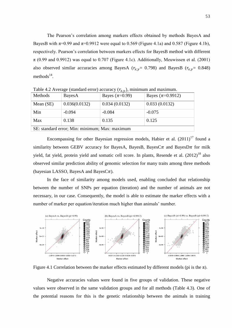
53

The Pearson’s correlation among markers effects obtained by methods BayesA and

BayesB with π=0.99 and π=0.9912 were equal to 0.569 (Figure 4.1a) and 0.587 (Figure 4.1b),

respectively. Pearson’s correlation between markers effects for BayesB method with different

π (0.99 and 0.9912) was equal to 0.707 (Figure 4.1c). Additionally, Meuwissen et al. (2001)

also observed similar accuracies among BayesA (𝑟𝑥,𝑦= 0.798) and BayesB (𝑟𝑥,𝑦= 0.848)

methods14

.

Table 4.2 Average (standard error) accuracy (𝑟𝑥,𝑦), minimum and maximum.

Methods BayesA Bayes (𝜋=0.99) Bayes (𝜋=0.9912)

Mean (SE) 0.036(0.0132) 0.034 (0.0132) 0.033 (0.0132)

Min -0.094 -0.084 -0.075

Max 0.138 0.135 0.125

SE: standard error; Min: minimum; Max: maximum

Encompassing for other Bayesian regression models, Habier et al. (2011)17

found a

similarity between GEBV accuracy for BayesA, BayesB, BayesC𝜋 and BayesD𝜋 for milk

yield, fat yield, protein yield and somatic cell score. In plants, Resende et al. (2012)18

also

observed similar prediction ability of genomic selection for many traits among three methods

(bayesian LASSO, BayesA and BayesC𝜋).

In the face of similarity among models used, enabling concluded that relationship

between the number of SNPs per equation (iteration) and the number of animals are not

necessary, in our case. Consequently, the model is able to estimate the marker effects with a

number of marker per equation/iteration much higher than animals’ number.

Figure 4.1 Correlation between the marker effects estimated by different models (pi is the π).

Negative accuracies values were found in five groups of validation. These negative

values were observed in the same validation groups and for all methods (Table 4.3). One of

the potential reasons for this is the genetic relationship between the animals in training

54

population and validation group. A high relationship between both groups is favorable for

accuracy of prediction. However, we did not observe this behavior, founding average

correlation among the accuracy and relationship between animals from validation and training

group equal to -0.148.

As a part of quest for justification of negative and low accuracies, Hayes et al.

(2009)19

cited parameters that the accuracy of GEBV is dependent, such as level of linkage

disequilibrium (LD) between the markers and the QTL; the number of animals with

phenotypes and genotypes in the training population; and, additionally, the relationship

between animals.

Accuracies of GEBV equal to 0.85 were achieved in the level of LD between adjacent

markers greater than 0.2 (allelic frequency correlation, r² ≥ 0.2)14

. In this study using Santa

Inês breed, and in other Ovis aries breeds, a low LD with average r² equal to 0.166 was found.

Thus, an additional reason for the low average accuracy observed is the low average LD.

The third potential reason is the size of the training population that might influence the

accuracy. Probably, the small size of the training group does not allow proper makers effects

estimation. The definition of records number is depended on trait heritability; greater

heritability, fewer records are required 19

. In this study, high genomic heritability for RFI was

observed (0.75). For traits with heritability near 0.7, the number of phenotypic records

required to achieve a desired accuracy of GEBV was approximately 2,000 20

. Therefore, it is

likely that the number of animals was not sufficient.

55

Table 4.3 Correlation between genomic estimated breeding value and adjusted phenotype by

group training-validation between methods.

Gt-v BayesA BayesB

(π=0.99)

BayesB

(π=0.9912) 𝑟𝑥,𝑦

1 0.038 0.017 0.002 0.0018

2 0.061 0.075 0.084 -0.0020

3 0.040 0.043 0.028 0.0004

4 0.064 0.077 0.069 -0.0062

5 0.128 0.123 0.125 0.0025

6 0.087 0.076 0.078 -0.0011

7 0.071 0.060 0.058 -0.0012

8 -0.094 -0.084 -0.075 0.0033

9 -0.016 0.012 0.000 -0.0029

10 -0.052 -0.060 -0.060 -0.0012

11 -0.029 -0.029 -0.013 -0.0063

12 0.054 0.064 0.076 -0.0040

13 -0.002 0.012 0.016 -0.0012

14 0.065 0.048 0.045 0.0020

15 0.138 0.135 0.109 -0.0040

16 0.012 -0.005 0.011 0.0021

17 0.039 0.038 0.039 -0.0025

18 0.023 0.007 0.007 -0.0035

19 0.052 0.046 0.032 -0.0017

Gt-v: group training-validation; rx,y: average of relationship of animals

The final hypothesis for negative and low average accuracies was the average of the

relationship between all animals that was low, close to zero. The average genetic relationship

between animals (standard deviation) was 0.0011 (0.06340), with minimum and maximum

values equal to -0.1353 and 0.9341, respectively. This finding is also presented in Figure 4.2

as a heatmap of genetic relationship among animals. Hayes et al. (2009) 21

verified the GEBV

accuracy using different training and validation groups. For instance, they used two dairy

cattle breeds data (Jersey and Holstein). The marker effects were estimated by the BayesA

with Holstein breed training data and were found accuracies of GEBV for milk production

equal to 0.59 and 0.37 for Holstein and Jersey group-validation, respectively 21

. Using Jersey

breed data training were observed accuracies for milk production equal to 0.59 and -0.02 for

Jersey and Holstein group-validation, respectively 21

.

Based on the results and computing time required for the analyses, the better model

was the BayesA as it presented lower average (1,013 seconds) than BayesB with π=0.99

(2,232 seconds) and π=0.9912 (2,268 seconds).

56

Figure 4.2 Heatmap of genetic relationship between animals.

4.4 Conclusion

The limiting factor for obtaining medium/high accuracy in GS was the low

relationship between animals and the size of training population. Consequently, for the

marker effects estimation is necessary to systematically training population chosen with a

significant number of animals and minimum of the relationship between animals, or develop

methods that optimize both challenges.

References

1. Herd, R. M., Archer, J. A. & Arthur, P. F. Reducing the cost of beef production through genetic

improvement in residual feed intake : Opportunity and challenges to application The online

version of this article , along with updated information and services , is located on the World

Wide Web at : R. J. Anim. Sci. 81, E9–E17 (2003).

2. Hegarty, R. S., Goopy, J. P., Herd, R. M. & McCorkell, B. Cattle selected for lower residual

feed intake have reduced daily methane production. J. Anim. Sci. 85, 1479–1486 (2007).

3. Koch, R. M., Swiger, L. A., Chambers, D. & Gregory, K. E. Efficiency of feed use in beef

cattle. J. Anim. Sci. 22.2, 486–494 (1963).

4. Bolormaa, S. et al. Accuracy of prediction of genomic breeding values for residual feed intake

and carcass and meat quality traits in Bos taurus, Bos indicus, and composite beef cattle. J.

Anim. Sci. 91, 3088–3104 (2013).

5. Archer, J. a, Arthur, P. F., Herd, R. M., Parnell, P. F. & Pitchford, W. S. Optimum postweaning

test for measurement of growth rate , feed intake , and feed efficiency in British breed cattle. J.

Anim. Sci. 75, 2024–2032 (1997).

57

6. Arthur, P. F., Renand, G. & Krauss, D. Genetic and phenotypic relationships among different

measures of growth and feed efficiency in young Charolais bulls. Livest. Prod. Sci. 68, 131–

139 (2001).

7. VanRaden, P. M. Efficient methods to compute genomic predictions. J. Dairy Sci. 91, 4414–23

(2008).

8. Legarra, a, Aguilar, I. & Misztal, I. A relationship matrix including full pedigree and genomic

information. J. Dairy Sci. 92, 4656–4663 (2009).

9. Misztal, I., Legarra, A. & Aguilar, I. Computing procedures for genetic evaluation including

phenotypic, full pedigree, and genomic information. J. Dairy Sci. 92, 4648–4655 (2009).

10. Aguilar, I. et al. Hot topic: a unified approach to utilize phenotypic, full pedigree, and genomic

information for genetic evaluation of Holstein final score. J. Dairy Sci. 93, 743–52 (2010).

11. Purcell, S. PLINK (1.07) Documentation. 283 (2010). doi:10.1525/mp.2010.27.5.337

12. VanRaden, P. M. et al. Invited review: reliability of genomic predictions for North American

Holstein bulls. J. Dairy Sci. 92, 16–24 (2009).

13. de los Campos, G., Hickey, J. M., Pong-Wong, R., Daetwyler, H. D. & Calus, M. P. L. Whole-

genome regression and prediction methods applied to plant and animal breeding. Genetics 193,

327–345 (2013).

14. Meuwissen, T. H. E., Hayes, B. J. & Goddard, M. E. Prediction of total genetic value using

genome-wide dense marker maps. Genetics 157, 1819–1829 (2001).

15. Fernando, R. L. & Garrick, D. J. in Genome-Wide Association Studies and Genomic Prediction

1, 1–565 (2013).

16. Heidelberger, P. & Welch, P. D. Simulation run length control in the presence of an initial

transient. Oper. Res. 31, 1109–1144 (1983).

17. Habier, D., Fernando, R. L., Kizilkaya, K. & Garrick, D. J. Extension of the bayesian alphabet

for genomic selection. BMC Bioinformatics 12, 186 (2011).

18. Resende, M. F. R. et al. Accuracy of Genomic Selection Methods in a Standard Data Set of

Loblolly Pine (Pinus taeda L.). Genetics 190, 1503–1510 (2012).

19. Hayes, B. J., Bowman, P. J., Chamberlain, A. J. & Goddard, M. E. Genomic selection in dairy

cattle: progress and challenges. J. Dairy Sci. 92, 433–443 (2009).

20. Goddard, M. Genomic selection: Prediction of accuracy and maximisation of long term

response. Genetica 136, 245–257 (2009).

21. Hayes, B. J., Bowman, P. J., Chamberlain, A. C., Verbyla, K. & Goddard, M. E. Accuracy of

genomic breeding values in multi-breed dairy cattle populations. Genet. Sel. Evol. 41, 51

(2009).

58

59

5. FINAL CONSIDERATION

The development and enhancement of reproductive and molecular technologies have

allowed the acceleration of genetic progress through the genetic evaluation of young

individuals to a certain accuracy, even in characteristics of low heritability, of difficult and

onerous measurement or delayed measurement in the life of the animal. This study represents

an initial step for genomic-quantitative studies and genomic selection for feed efficiency traits

in domestic sheep. First, we study the genome structural by mapping of linkage

disequilibrium, concluding that is necessary high density of markers panel for genomic

approaches application in Santa Inês sheep. For the residual feed intake trait, we observed

high genomic heritability, suggesting greater opportunity and results for animal breeding than

other feed efficiency traits. For the comprehension of genomic selection used, it is still

necessary to systematically collect phenotypic and genotypic information to include a larger

number of animals in the training group, and with at least of animal’s relationship for a

possible improvement in accuracy; and finally, the analysis of costs and revenues associated

with the characteristics of interest using genomic information.

60

61

SUPLEMENTARY FIGURES

Supplementary figure 2.1 LD measured by r² plotted as a function of intermarker distance

(Mb) for chromosomes.

62

Supplementary figure 2.2 LD measured by D’ plotted as a function of intermarker distance

(Mb) for chromosomes.

63 SUPLEMENTARY TABLES Supplementary File 3.1 SNP associated, respectively gene, chromosome, position, SNP effect and bayes factor.

Trait SNP_novo Ensemble (Gene) Gene name Position Effect % VarGen alelo BP

RFI rs414735594 ENSOARG00000026794

uncaracterized

protein 26:28702214 -0.01147 0.00118947 [A/G] 32.7189995

RFI rs410141696 6:85018309 0.01558 0.00132226 [T/C] 27.7443349

RFI rs430321012 7:98174186 0.01146 0.00099079 [T/C] 22.2047013

RFI rs402761680 ENSOARG00000015069 MTFR2 8:61268758 -0.008097 0.00076862 [T/C] 17.9383416

RFI rs411518548 ENSOARG00000003036

uncaracterized

protein 15:49746734 0.00572 0.00065487 [A/G] 16.6947528

RFI rs411784503 3:198973527 -0.005693 0.00061347 [T/C] 15.331909

RFI rs428751386 ENSOARG00000015133 CEP95 11:48125112 -0.004115 0.00051909 [A/G] 12.3736078

RFI rs408272283 23:38230104 -0.004408 0.00046255 [A/G] 10.9023091

RFI rs409559449 5:310744 -0.003667 0.00044356 [T/C] 10.9023091

RFI rs413247589 3:203798865 0.003736 0.00044369 [T/C] 10.5375083

RFI rs408365913 ENSOARG00000012755 GDA 2:63837976 -0.004148 0.00042388 [A/G] 9.87495876

RFI rs419463225 ENSOARG00000003379 EFCAB11 7:98396585 -0.005159 0.00047014 [T/C] 9.75535538

RFI s56827.1 4:114893675 -0.003772 0.00042481 [A/G] 9.45749343

RFI rs412816959 8:7457271 -0.002997 0.00037407 [A/G] 8.97251609

RFI rs413057852 22:32429371 0.002953 0.00036108 [T/C] 8.51520417

RFI rs417128974 ENSOARG00000006995 FCHSD2 15:50781754 -0.003329 0.000363 [T/C] 8.49185668

RFI rs408441367 11:48556687 -0.002807 0.00035263 [T/C] 8.24731882

RFI rs406251433 8:90234353 -0.00416 0.00040341 [T/C] 8.05017301

RFI rs398957969 4:92688260 0.002717 0.00033697 [A/G] 7.85375067

RFI rs419579453 ENSOARG00000014668 ZFYVE16 5:77888494 0.002772 0.00031847 [T/C] 7.17760618

RFI OAR8_76092068.1 8:76092068 0.002335 0.0003207 [T/C] 7.0865838

RFI rs411082902 2:76748382 -0.003911 0.00035523 [A/G] 6.99571734

RFI rs414518818 23:22393678 0.002409 0.00029264 [T/C] 6.98436998

RFI s23148.1 9:15350447 -0.002208 0.00030361 [T/C] 6.65635005

RFI rs405076950 4:89310177 -0.002179 0.00027676 [A/C] 6.4088586

RFI OAR20_46803189.1 20:46803189 -0.003276 0.00031889 [A/G] 6.17369595

RFI rs415988359 4:9108090 0.003658 0.000323117 [A/G] 6.17369595

RFI OAR5_79829554.1 5:79829554 -0.002146 0.000244831 [T/C] 6.0955414

RFI rs400802261 ENSOARG00000005292 CPA5 4:94145887 -0.002033 0.000256574 [T/C] 6.00636402

RFI rs401602228 5:17836037 -0.002204 0.00026885 [A/C] 5.76190476

RFI rs403066959 11:51650294 -0.001809 0.000255154 [A/G] 5.69543147

RFI OAR1_153662211.1 1:153662211 -0.002517 0.000257036 [A/G] 5.61798584

64 Trait SNP_novo Ensemble (Gene) Gene name Position Effect % VarGen alelo BP

RFI rs400411648 4:108494061 -0.002111 0.000239742 [T/C] 5.58482992

RFI rs414816492 ENSOARG00000003012 PLEKHG1 8:74555627 -0.001732 0.00022629 [A/C] 5.36432638

RFI OAR15_40099623.1 15:40099623 -0.00208 0.00023788 [A/G] 5.23246999

RFI rs425134950 ENSOARG00000020315 MAN1A2 1:94050486 -0.001498 0.000207985 [A/G] 4.9588365

RFI OAR11_27752920.1 11:27752920 0.001819 0.000222699 [A/G] 4.9588365

RFI OAR16_72265538.1 16:72265538 -0.002618 0.000248341 [T/C] 4.81711409

RFI rs423570605 ENSOARG00000013828 1:60733952 0.001719 0.000200672 [T/C] 4.53482535

RFI rs417223706 ENSOARG00000010362 MYL12A 23:37749930 0.001597 0.000191129 [T/C] 4.30794115

RFI rs411012150 13:36682642 0.001572 0.000182584 [T/G] 4.2648378

RFI rs160106606 ENSOARG00000009032 uncaracterized

protein

5:60421059 -0.001674 0.000184751 [T/G] 4.2648378

RFI rs425904136 8:7501857 0.00132 0.000180834 [T/C] 4.24329961

RFI rs415141804 4:92807686 -0.001341 0.000176504 [T/C] 4.23253389

RFI rs410904559 4:840726 0.002257 0.000222249 [A/G] 4.18949343

RFI OAR9_68618966.1 9:68618966 0.001343 0.000185358 [T/C] 4.18949343

RFI s69512.1 15:21926139 0.00135 0.000177444 [T/C] 4.16798666

RFI rs398217340 ENSOARG00000013809 LURAP1L 2:80731070 0.001516 0.000194972 [A/C] 4.1035201

RFI OAR5_77162689.1 5:77162689 0.0015 0.00016696 [A/C] 4.09278351

RFI OAR8_69071490.1 8:69071490 -0.001309 0.000167117 [A/G] 4.01768991

RFI rs402543445 19:58097089 -0.001929 0.000180793 [A/G] 3.91060291

RFI rs426937018 8:72055247 0.001235 0.00016819 [A/G] 3.86783042

RFI OAR15_52395182.1 15:52395182 -0.00141 0.000172353 [A/G] 3.82509348

RFI OARX_16441119.1 27:16441119 0.001533 0.000169102 [A/G] 3.82509348

RFI s03769.1 2:22928115 0.001148 0.000158432 [A/C] 3.7610546

RFI rs421479854 2:63675988 -0.001421 0.000172028 [T/C] 3.75038921

RFI rs419342821 ENSOARG00000014403

uncaracterized

protein 9:35529619 -0.001169 0.000163295 [T/G] 3.73972603

RFI rs406967914 4:94552733 0.001277 0.000162703 [T/C] 3.72906506

RFI OAR26_32903035.1 26:32903035 -0.001263 0.000158684 [A/G] 3.6757934

RFI rs424506880 10:52459290 0.001179 0.000155123 [T/C] 3.6651457

RFI rs405615582 ENSOARG00000013544 RIC1 2:73333474 -0.001332 0.00015436 [T/C] 3.60130583

RFI rs426940450 ENSOARG00000023774

uncaracterized

protein 20:43161083 0.002047 0.000184428 [T/C] 3.60130583

RFI rs415294045 ENSOARG00000013596 COBL 4:4713517 0.001137 0.000149133 [T/C] 3.60130583

RFI s07134.1 15:5988222 0.001197 0.000160527 [T/G] 3.59067358

RFI rs414207473 ENSOARG00000007560 ARHGAP42 15:7536215 -0.001291 0.000151754 [A/C] 3.59067358

65 Trait SNP_novo Ensemble (Gene) Gene name Position Effect % VarGen alelo BP

RFI rs426186644 ENSOARG00000025287 uncaracterized

protein 5:6895007 -0.001157 0.000153254 [T/C] 3.58004352

RFI rs426186644 ENSOARG00000001029 uncaracterized

protein 5:6895007 -0.001157 0.000153254 [T/C] 3.58004352

RFI OAR12_8785706.1 12:8785706 -0.001219 0.000145048 [A/G] 3.56941567

RFI rs420380888 2:9877191 0.001078 0.000164689 [A/G] 3.52692626

RFI rs416863154 ENSOARG00000004438 uncaracterized

protein 8:81812309 -0.001389 0.000160036 [A/G] 3.49508231 RFI rs415843943 ENSOARG00000002063 SRRM4 17:55842659 0.001182 0.000150063 [A/C] 3.47386399

RFI OAR26_32961768.1 26:32961768 -0.001201 0.000155195 [A/G] 3.47386399

RFI rs413139541 ENSOARG00000025200 4:718077 -0.001841 0.000174847 [A/G] 3.47386399 RFI rs399102597 ENSOARG00000011518 PAX5 2:51529698 0.001336 0.000155489 [T/C] 3.45265446

RFI rs423217515 5:95970638 0.001232 0.00015919 [T/C] 3.44205298

RFI s71989.1 2:23659780 -0.001461 0.000146422 [A/G] 3.4314537

RFI rs411475019 1:205107119 -0.001419 0.00014595 [A/G] 3.36790404

RFI rs423531461 1:70855490 0.001401 0.000157159 [T/C] 3.3573201

RFI rs414345721 10:74465731 0.001004 0.000144667 [T/C] 3.18827415

RFI rs416676032 5:95329244 0.001 0.000130589 [A/G] 3.18827415

RFI OAR5_112405141.1 5:112405141 -0.001056 0.00013993 [T/C] 3.16718266

RFI rs412019471 ENSOARG00000026185 uncaracterized

protein 23:36854999 0.001368 0.000145189 [T/C] 3.16718266

RFI rs407100968 12:45742771 -0.000996 0.000134846 [A/G] 3.13556175

RFI rs415267900 ENSOARG00000016117 uncaracterized

protein 1:68632937 0.001404 0.000146856 [T/C] 3.1039604

RFI rs399135205 3:9958035 -0.001217 0.000140856 [A/G] 3.09343096

RFI OAR4_41049923.1 4:41049923 -0.001643 0.000155002 [A/G] 3.06185567

RFI rs403391311 23:22105490 0.0009791 0.000132935 [A/G] 3.06185567

RFI rs401422903 7:59408108 -0.001127 0.000137557 [T/C] 3.05133491

RFI rs411315526 10:64913571 -0.0009853 0.000130541 [T/C] 3.03029991

66 Trait SNP_novo Ensemble (Gene) Gene name Position Effect % VarGen alelo BP

FE rs402836082 ENSOARG00000011009

uncaracterized

protein 11:9074516 0.0003909 0.000142585 [A/G] 3.47386399

FE rs408501145 ENSOARG00000005184 PIK3C3 23:14088280 0.0006795 0.00013288 [A/C] 3.29386237

FE rs412052666 13:70886211 -0.0004808 0.000150472 [A/G] 3.72906506

FC rs416210172 1:53710321 0.01949 0.002458726 [A/G] 8.76096658

FC rs430136740 ENSOARG00000020436 SLCO1C1 3:193827830 -0.00874 0.000940729 [A/G] 5.07905803

FC rs406111016 ENSOARG00000020821

uncaracterized

protein 7:46878437 0.008686 0.001035656 [A/G] 4.751834

FC rs425422822 20:46556750 0.006286 0.00075029 [T/C] 3.89990645

FC rs417293333 23:44559717 -0.005761 0.000630313 [T/C] 3.64385692

FC rs402836082 ENSOARG00000011009

uncaracterized

protein 11:9074516 -0.005047 0.000540339 [A/G] 3.62257697

FC 19:1206663 0.005074 0.000544214 [T/G] 3.55879001

FC rs422431427 ENSOARG00000008837

uncaracterized

protein 16:31882270 0.007645 0.001079394 [T/C] 3.46325812

FC rs428620176 2:236977003 0.005263 0.000610997 [T/C] 3.4314537

FC rs406809081 3:24374242 -0.005074 0.000579704 [T/C] 3.41026172

FC rs402039066 5:34773855 -0.004339 0.000442463 [T/C] 3.241041

FC s36178.1 17:13746553 0.004149 0.000403458 [A/G] 3.17772732

FC rs429351668 ENSOARG00000013534 MYOC 12:37251694 -0.004164 0.000434504 [A/G] 3.1039604

FC rs410797913 2:140622573 -0.003967 0.000389464 [A/G] 3.1039604

FC OARX_11655327.1 27:11655327 0.004325 0.000457875 [T/C] 3.04081633

FC rs421641135 ENSOARG00000013390 GIPC2 1:53875325 0.004139 0.000420154 [A/G]

3.01978566

RFI rs423726969 5:528815 0.001044 0.000137024 [T/C] 3.29386237

RFI rs426828423 13:13066280 0.0011 0.000141806 [T/C] 3.262163

RFI rs424765042 4:10206259 0.001668 0.000162124 [T/C] 3.21992772