Embed Size (px)
Citation preview

STRUCTURAL HEALTH MONITORING SYSTEMS
FOR CIVIL AND ARCHITECTURAL STRUCTURES: LVDT-TAUT-WIRE BASELINES, CRACK MONITORING DEVICES,
& STRAIN BASED DEFLECTION MONITORING ALGORITHMS.
Gaur P. Johnson
Ian N. Robertson
Research Report UHM/CEE/07-02 February 2007
UNIVERSITY OF HAWAIICOLLEGE OF ENGINEERING
D
EPARTMENT OF
C
IVIL AND
E
NVIRONMENTAL
E
NGINEERING

ii

iii
ACKNOWLEDGMENTS
This report is based on a Ph.D. Dissertation prepared by Gaur Johnson under the direction
of Ian Robertson at the Department of Civil Engineering at the University of Hawaii at
Manoa.
The authors would like to thank the following projects which helped to make this report
possible:
• Robertson, I. (P.I.) "Instrumentation and Long-Term Monitoring of the H3 North
Halawa Valley Viaduct", funded by FHWA and Hawaii State DOT, 94-04.
• Robertson, I. (P.I.) "Seismic Instrumentation and Monitoring of the Kealakaha
Stream Bridge", funded by FHWA and Hawaii State DOT, 00-05.
• Robertson, I. (P.I.) "Testing of Prestressed Concrete Beams Repaired with Carbon
Fiber Reinforced Polymers", funded by Hawaii State DOT, 00-01.
• Riggs, H.R. (P.I.), Ian Robertson (co-P.I.) Si-Hwan Park (co-P.I.), 'Instrumenting
and Monitoring the Performance of the FRP Shear Strengthening of the Salt Lake
Boulevard Bridge,' FHWA Innovative Bridge Research and Construction program,
November 2003 - October 2008.
Thank you to all the faculty, staff, and fellow graduate students who have helped through
the process, including but by no means limited to: Dr. Ian Robertson, Dr. H. Ronald
Riggs, Dr. Si-Hwan Park, Dr. David Ma, Dr. Ronald Knapp, Dr. Craig Newtson, Dr.

iv
Arthur Chiu, Gary Chock, Miles Wagner, Andy Oshita, Janis Kusatsu, Bhavna Sharma,
Huiping Cheng, Jiabao Chen, Jinghai Yang, Huiyun Zhang, Kainoa Aki, Derek
Yonemura, Justin Nii, Wesley Furuya, Brian Enomoto, Martin & Chock, Nagamine
Okawa Engineers, and Iwamoto & Associates.

v
ABSTRACT
In this age of computers and electronics, we become increasingly aware of all the new
information we can collect about our surroundings. The medical industry has fully
embraced the use of this technology to help diagnose problems with our health. The civil
engineering profession is only now beginning the steps toward using structural health
monitoring (SHM) for the purpose of extending the productive lives of our infrastructure.
The ubiquitous use of SHM will reap the benefit of providing a rational method to
prioritize expenditure allocation to maintain our deteriorating facilities. Since SHM is far
from ubiquitous, the lessons learned during any instrumentation program provide a
significant contribution to the SHM field.
This dissertation begins by showing structural engineers a few of the tools of the trade
that can be used in a SHM program. To help open the instrumentation world to engineers
and scientists, an example of the process by which to design an economical crack gauge
is discussed. This dissertation also contributes new information to the SHM field. First,
a simple design process for an LVDT-Taut-Wire baseline system that measures vertical
deflections on long and short span beams is established. Second, a method by which to
pre-determine the magnitude of expected error caused by real data for a strain based
deflection monitoring algorithm is presented. Both of these contributions will help to
more quickly design SHM systems and provide the user reasonable confidence of the
systems performance before the system is installed. Finally, a brief discussion of how
some of the key lessons learned will be incorporated into four SHM projects is presented.

vi

vii
TABLE OF CONTENTS
Acknowledgments.............................................................................................................. iii
Abstract ............................................................................................................................... v
TABLE OF CONTENTS.................................................................................................. vii
LIST OF TABLES.......................................................................................................... xvii
LIST OF FIGURES ......................................................................................................... xix
Chapter 1. INTRODUCTION TO STRUCTURAL HEALTH MONITORING......... 1
1.1 General Purpose .................................................................................................. 1
1.2 Literature Review................................................................................................ 5
Chapter 2. AVAILABLE MEASUREMENT METHODOLOGIES........................... 9
2.1 Overall Data Acquisition Systems ...................................................................... 9
2.2 Linear Variable Differential Transformer (LVDT): ......................................... 10
2.2.1 Ratiometric Wire Configuration ............................................................... 12
2.2.2 Open Wire Configuration ......................................................................... 12
2.2.3 Influence of Cable Length ........................................................................ 13
2.2.4 Sensitivity Correction Factor (SCF) ......................................................... 14

viii
2.2.5 Limitations for Structural Health Monitoring........................................... 17
2.3 Strain Gauges .................................................................................................... 18
2.3.1 Types of Strain Gauges............................................................................. 18
2.3.1.1 Electrical Resistance Strain Gauges...................................................... 19
2.3.1.2 Fiber Optic Strain Gauges..................................................................... 28
2.3.1.3 Vibrating Wire Strain Gauges............................................................... 35
2.3.2 Thermal Effects and Considerations for Strain Gauges............................ 36
2.3.2.1 Thermal Output Compensation Techniques ......................................... 39
2.3.3 Structural Health Monitoring Strain Gauge Comparison ......................... 46
2.3.3.1 Electrical Resistance Strain Gauges...................................................... 46
2.3.3.2 Fiber Optic Strain Gauges..................................................................... 47
2.3.3.3 Vibrating Wire Strain Gauges............................................................... 49
Chapter 3. LVDT-TAUT-WIRE BASELINE DEFLECTION SYSTEM DESIGN.. 51
3.1 Literature Review.............................................................................................. 51
3.2 University of Hawaii System Design Process .................................................. 57
3.2.1 In Laboratory Prestressed Concrete T-Beam Testing............................... 58

ix
3.2.2 North Halawa Valley Viaduct (H3 Freeway) Field Installation ............... 62
3.2.3 Hanapepe River Bridge Load Test Field Installation ............................... 65
3.3 System Sizing Considerations........................................................................... 68
3.3.1 Implemented System Comparisons........................................................... 68
3.3.2 Suggested Design Process......................................................................... 73
Chapter 4. WHEATSTONE BRIDGE DEVICE DESIGN........................................ 77
4.1 Background....................................................................................................... 77
4.2 Crack Gauge Device ......................................................................................... 78
4.2.1 Design Basis.............................................................................................. 79
4.2.2 Physical Specifications ............................................................................. 80
4.2.3 Estimating Crack Mouth Opening Displacement (CMOD) Resolution ... 84
4.3 Rotation Monitoring by Deflection Device ...................................................... 87
4.3.1 Design Basis.............................................................................................. 87
4.3.2 Physical Specifications ............................................................................. 88
4.3.3 Estimating Displacement Resolution........................................................ 91
Chapter 5. STRAIN GAUGE BASED DEFLECTED SHAPE CALCULATION.... 93

x
5.1 Literature Review.............................................................................................. 93
5.2 General Methodology ....................................................................................... 96
5.3 Curvature to Displacement (C2D) Derivation .................................................. 97
5.4 C2D Method Matlab™ Implementation:........................................................ 101
5.4.1 RISA-2D Strain Input ............................................................................. 102
5.4.2 Evaluated Loading Scenarios.................................................................. 104
5.4.3 Matlab Implementation Scenario 1MoCS .............................................. 106
5.4.4 Matlab Implementation Scenario 1MoAS .............................................. 107
5.4.5 Matlab Implementation Scenario 1QPoCS............................................. 109
5.4.6 Matlab Implementation Scenario 1DLoM2............................................ 112
5.4.7 Matlab Implementation Scenario 1DLoNb............................................. 113
5.4.8 Small Scale Implimentation.................................................................... 115
5.4.8.1 Static Test............................................................................................ 116
5.4.8.2 Dynamic Tests .................................................................................... 119
5.5 Conclusions..................................................................................................... 121
5.5.1 Comments on Curvature Estimation....................................................... 122

xi
5.5.2 Comments on Deflected Shape............................................................... 122
5.5.3 Comments on Real Data Implementation ............................................... 123
Chapter 6. ANALYSIS OF STRAIN GAGE BASED DEFLECTED SHAPE
CALCULATIONS.......................................................................................................... 125
6.1 Background..................................................................................................... 125
6.2 Error Sources in Real Data used in C2D Method ........................................... 126
6.2.1 Measurement Round Off......................................................................... 127
6.2.1.1 Matlab Implementation Scenario 1MoCS .......................................... 128
6.2.1.2 Matlab Implementation Scenario 1MoAS .......................................... 130
6.2.1.3 Matlab Implementation Scenario 1QPoCS......................................... 133
6.2.1.4 Matlab Implementation Scenario 1DLoM2........................................ 136
6.2.1.5 Matlab Implementation Scenario 1DLoNb......................................... 138
6.2.2 Signal Noise Characteristics ................................................................... 141
6.2.3 Sample of Real Strain Data..................................................................... 143
6.3 Analysis of Error Propagation in C2D Method .............................................. 144
6.3.1 Error at Individual Sensors ..................................................................... 145

xii
6.3.1.1 Single Beam Section ........................................................................... 145
6.3.1.2 Entire Beam ........................................................................................ 148
6.3.2 Error at Multiple Sensors ........................................................................ 151
6.3.2.1 Deflected Shape of the Entire Beam................................................... 152
6.3.2.2 Dynamic or Multiple Measurements .................................................. 158
6.4 Comments on Error Reduction Methods for C2D Method............................. 166
6.4.1 Post Processing Data Averaging............................................................. 166
6.4.1.1 Static Measurements ........................................................................... 167
6.4.1.2 Dynamic Measurements...................................................................... 168
6.4.2 C2D Method Adaptations ....................................................................... 173
6.4.2.1 Number of Beam Sections .................................................................. 174
6.4.2.2 Alternate Curvature Estimate Implementations.................................. 174
6.4.2.3 Multiple Implementation Comparison................................................ 174
6.5 Conclusions..................................................................................................... 175
Chapter 7. SHM DURING HANAPEPE RIVER BRIDGE LOAD TESTING....... 177
7.1 Background..................................................................................................... 177

xiii
7.2 Bridge SHM Instrumentation.......................................................................... 177
7.2.1 Vertical Deflection.................................................................................. 180
7.2.2 Horizontal Deflection.............................................................................. 184
7.2.3 Crack Mouth Opening Displacement...................................................... 184
7.2.4 Rotation at Lihue Pier Support ............................................................... 190
7.3 Data Acquisition and Processing .................................................................... 192
7.3.1 Optical Survey ........................................................................................ 192
7.3.2 Temperature Effects................................................................................ 193
7.4 Load Test Program.......................................................................................... 196
7.4.1 Truck Loads ............................................................................................ 196
7.4.2 Static Loading ......................................................................................... 198
7.4.3 Dynamic Loading.................................................................................... 200
7.5 Load Test Results............................................................................................ 200
7.5.1 Vertical Deflections ................................................................................ 200
7.5.1.1 Load Series 1....................................................................................... 200
7.5.1.2 Load Series 2 and 3............................................................................. 202

xiv
7.5.1.3 Load Series 4 and 5............................................................................. 203
7.5.1.4 Load Series 6....................................................................................... 204
7.5.2 Horizontal Deflection.............................................................................. 206
7.5.3 Rotation at Lihue Piers............................................................................ 207
7.5.4 Crack Mouth Opening Displacements .................................................... 209
7.5.4.1 General................................................................................................ 209
7.5.5 Dynamic Response.................................................................................. 212
7.6 Conclusions about Bridge and SHM System.................................................. 215
Chapter 8. OTHER PLANNED SHM IMPLEMENTATIONS............................... 217
8.1 North Halawa Valley Viaduct (NHVV) ......................................................... 217
8.1.1 Background............................................................................................. 217
8.1.2 Results: LVDT-Taut-Wire Baseline System .......................................... 218
8.1.3 Results: Strain Gauge Based C2D Methodology.................................... 220
8.2 Kealakaha Stream Bridge Seismic Instrumentation ....................................... 221
8.2.1 Background............................................................................................. 221
8.2.2 LVDT-Taut-Wire Baseline System ........................................................ 222

xv
8.2.3 C2D Methodology .................................................................................. 223
8.3 Salt Lake Boulevard – Halawa Stream Bridge: Shear Retrofit....................... 225
8.3.1 Background............................................................................................. 225
8.3.2 Planned Instrumentation ......................................................................... 225
Chapter 9. SUMMARY AND CONCLUSIONS ..................................................... 227
APPENDIX..................................................................................................................... 231
REFERENCES ............................................................................................................... 261

xvi

xvii
LIST OF TABLES
Table 2.1. Strain Gauge Behavior Sensitivities. .............................................................. 38
Table 3.1. Summary of LVDT Core-Induced Baseline Displacement. ........................... 69
Table 3.2. Estimated Error at LVDTs Due to Friction with LVDT Core........................ 72
Table 5.1. Matlab™ Based C2D Method Evaluation Scenarios. ................................... 105
Table 5.2. Curvature Observations Used in C2D Program............................................ 105
Table 6.1. Curvature Input for Three Span Continuous Beam. ..................................... 128
Table 6.2. Statistical Characteristics of Strain Error Based on Average Strain Value. .. 144
Table 6.3. Positive Error Combinations Calculated by Superposition. ......................... 153
Table 6.4. Alternating Direction Error Combinations Calculated by Superposition..... 153
Table 6.5. Small Scale Three Span Beam Signal Error Characteristics Summary........ 161
Table 7.1. Crack Gauge Details. .................................................................................... 190
Table 7.2. Truck Load Series. ........................................................................................ 199

xviii
xix
LIST OF FIGURES
Figure 2.2.1. LVDT Output [source: Trietily 1986, pg 69]. ............................................. 11
Figure 2.2.2. Effect of Sensitivity Correction Factor (SCF)............................................ 16
Figure 2.2.3. LVDT Sensitivity Correction Factor vs. Cable Length.............................. 16
Figure 2.3.1. Voltage Divider Circuit. ............................................................................. 20
Figure 2.3.2. Sample Calculation to Find Voltage Resolution (5µε measurement). ........ 21
Figure 2.3.3. Wheatstone Bridge Circuit. ........................................................................ 23
Figure 2.3.4. Long Lead Quarter Bridge Configuration. ................................................. 25
Figure 2.3.5. Thermal Output from an Electrical Resistance Strain Gauge [source:
Vishay 2005, pg 6]. ................................................................................................... 27
Figure 2.3.6. Fabry-Perot Fiber Optic Strain Gauge [source: Fiso 2006]........................ 29
Figure 2.3.7. Fabry-Perot Etalon [source: Drexel 2006]. ................................................ 30
Figure 2.3.8. Bragg Grating Gauge Methodology [source: Chiareli 1999]. .................... 31
Figure 2.3.9. Reflected Spectrum Changes due to Residual Strains [source: Wnuk 2005,
pg 5]. ......................................................................................................................... 34
Figure 2.3.10. Typical Structural Diurnal Response........................................................ 41

xx
Figure 2.3.11. Strain Gauge Output Change Due to α Mismatch Effects [source: Vishay
2005, pg 9]. ............................................................................................................... 44
Figure 3.1.1. Weighted Stretched Wire System [source: Stanton et al. 2003, pg 348]. ... 56
Figure 3.2.1. LVDT-Taut-Wire Installed on Pre-stressed Concrete Beam...................... 59
Figure 3.2.2. Live End Pulleys Installed on Prestressed Concrete Beam. ....................... 60
Figure 3.2.3. T-Beam Deflected Shapes. ......................................................................... 61
Figure 3.2.4. T-Beam capacity Curve.............................................................................. 61
Figure 3.2.5. NHVV Deflection Observed with LVDT-Taut-Wire Baseline System. ..... 64
Figure 3.2.6. Deflection Along the NHVV Span Varying with Time. ............................ 65
Figure 3.2.7. Abutment Span Elevation of Girder G-3: LVDT-Taut-Wire Baseline
System....................................................................................................................... 66
Figure 3.2.8. Bridge Cross-Section: LVDT-Taut-Wire Baseline Adjacent to Girder G-3.
................................................................................................................................... 67
Figure 3.2.9. Taut-Wire Baseline Dead (Left) and Live (Right) End Supports............... 67
Figure 3.3.1. Geometry of Deflection and Loads Applied to the Taut-Wire Catenary. .. 71
Figure 4.2.1. Crack Gauge Wheatstone Bridge Wiring Diagram. ................................... 81

xxi
Figure 4.2.2. Crack Gauge Design and Loading Diagram............................................... 82
Figure 4.2.3. Crack Gauge Installations........................................................................... 83
Figure 4.3.1. Deflection Gauge For Monitoring Pin Connection Rotation. .................... 89
Figure 4.3.2. Installed Gauges Monitoring Rotation of Pinned Connection at Pier. ....... 90
Figure 5.4.1. Three-Span Continuous Beam Modeled. ................................................. 103
Figure 5.4.2. Three-Span Continuous Beam Finite Element Model (4 Elements). ....... 103
Figure 5.4.3. Scenario 1MoCS: Curvature Estimation. ................................................. 106
Figure 5.4.4. Scenario 1MoCS: Deflection Comparison. .............................................. 107
Figure 5.4.5. Scenario 1MoAS: Curvature Estimation. ................................................. 108
Figure 5.4.6. Scenario 1MoAS: Deflection Comparison............................................... 109
Figure 5.4.7. Scenario 1QPoSC: Curvature Estimation................................................. 110
Figure 5.4.8. Scenario 1QPoCS: Deflection Comparison.............................................. 111
Figure 5.4.9. Scenario 1DLoM2: Curvature Estimation................................................ 112
Figure 5.4.10. Scenario 1DLoM2: Deflection Comparison........................................... 113
Figure 5.4.11. Scenario 1DLoNb: Curvature Estimation. ............................................. 114
Figure 5.4.12. Scenario 1DLoNb: Deflection Comparison. .......................................... 115

xxii
Figure 5.4.13. Static Loading Strains Obtained by Fabry-Perot Strain Gauges. ........... 117
Figure 5.4.14. C2D Static Results—Four Levels of Load. ............................................ 118
Figure 5.4.15. C2D Method Observations, Dynamic Response of Small Scale Beam. 120
Figure 5.4.16. C2D Calculated Deflection Based on the Theoretical Strains, Mode 1. 121
Figure 6.2.1. Scenario 1MoCS: C2D Curvature Comparison. ....................................... 129
Figure 6.2.2. Scenario 1MoCS: C2D Deflection Comparison....................................... 130
Figure 6.2.3. Scenario 1MoAS: C2D Curvature Comparison. ...................................... 131
Figure 6.2.4. Scenario 1MoAS: C2D Deflection Comparison. ..................................... 132
Figure 6.2.5. Scenario 1QPoCS: C2D Curvature Comparison...................................... 134
Figure 6.2.6. Scenario 1QPoCS: C2D Deflection Comparison. .................................... 135
Figure 6.2.7. Scenario 1DLoM2: C2D Curvature Comparison. .................................... 137
Figure 6.2.8. Scenario 1DLoM2: C2D Deflection Comparison. ................................... 138
Figure 6.2.9. Scenario 1DLoNb: C2D Curvature Comparison...................................... 139
Figure 6.2.10. Scenario 1DLoNb: C2D Deflection Comparison................................... 140
Figure 6.2.11. Strain Gauge Data Acquired for 18.69 seconds at 16 Hz (300 Data Points).
................................................................................................................................. 143
xxiii
Figure 6.3.1. Second Degree Polynomial Curvature Approximation: Error at One Gauge.
................................................................................................................................. 146
Figure 6.3.2. Third Degree Polynomial Rotation Approximation: Error at One Gauge.
................................................................................................................................. 147
Figure 6.3.3. Fourth Degree Polynomial Curvature Approximation: Error at One Gauge.
................................................................................................................................. 147
Figure 6.3.4. Curvature Error Based on One Measurement Location. .......................... 149
Figure 6.3.5. Rotation Error Based on One Measurement Location. ............................ 150
Figure 6.3.6. Displacement Error Based on One Measurement Location. .................... 151
Figure 6.3.7. Deflection Based on Multiple Positive Curvature Error Locations.......... 154
Figure 6.3.8. Deflection Based on Multiple Alternating (+/-) Curvature Error Locations.
................................................................................................................................. 156
Figure 6.3.9. All Possible Positive Error Combination Displacement Functions.......... 157
Figure 6.3.10. Expected Error Deflection Envelopes for the Small Scale Beam. ......... 162
Figure 6.3.11. LVDT Deflected Shape Observations. ................................................... 164
Figure 6.3.12. C2D Based Deflected Shape Observations. ........................................... 164
Figure 6.3.13. LVDT & C2D Maximum Measured Displacements.............................. 165

xxiv
Figure 6.3.14. C2D Error Envelope Comparison with LVDT and Support Measurements.
................................................................................................................................. 165
Figure 6.3.15. Comparison of Error Envelopes for Deflection at Location of an LVDT.
................................................................................................................................. 166
Figure 6.4.1. Before (Left) and After (Right) Averaging C2D Static Displacements. .. 168
Figure 6.4.2. Rectangular Averaging Windows Effects on Deflection. ........................ 170
Figure 6.4.3. Triangular Averaging Windows Effects on Deflection............................ 172
Figure 6.4.4. Comparison of Rectangular Averaging Windows for the Entire Beam. .. 173
Figure 7.2.1. Data Acquisition System. ......................................................................... 179
Figure 7.2.2. Elevation of Girder G-3 Showing LVDT-Taut-Wire Baseline Systems.. 180
Figure 7.2.3. LVDT-Taut-Wire Baseline System in Lihue Span. ................................. 181
Figure 7.2.4. LVDT-Taut-Wire Baseline System in Center Span. ................................ 181
Figure 7.2.5. Bridge Cross-Section Showing Baseline System Location...................... 182
Figure 7.2.6. Taut-Wire Baseline Dead (Left) and Live (Right) End Supports............. 183
Figure 7.2.7. LVDT-Taut-Wire Baseline LVDT Support Details. ................................ 183
Figure 7.2.8. Horizontal LVDT Measuring Deflection at Lihue Rocker Bearing. ........ 184

xxv
Figure 7.2.9. Crack Gauge on Downstream Elevation of Center Span. ........................ 185
Figure 7.2.10. Crack Gauges on Downstream Elevation of Lihue Span. ...................... 186
Figure 7.2.11. Crack Gauges on Upstream Elevation of Center Span........................... 186
Figure 7.2.12. Crack Gauges on Upstream Elevation of Lihue Span. ........................... 187
Figure 7.2.13. Crack Gauge 9 Adjacent to Visual Crack Monitor 3. ............................ 188
Figure 7.2.14. Typical Crack Gauge (10) on Mounting Tabs........................................ 189
Figure 7.2.15. Rotation Monitoring Gauge (1) on Waimea Side of Lihue Pier Bearing.
................................................................................................................................. 191
Figure 7.2.16. Rotation Monitoring Gauge (2) on Lihue Side of Lihue Pier Bearing... 191
Figure 7.3.1. Optical Survey Points. .............................................................................. 192
Figure 7.3.2. Thermal Compensation of Hanapepe River Bridge. ................................ 194
Figure 7.3.3. Thermocouple Locations on H3 North Halawa Valley Viaduct [Robertson
& Ingham 1999]. ..................................................................................................... 195
Figure 7.3.4. H3 North Halawa Valley Viaduct Daily Temperature Variation [Robertson
& Ingham 1999]. ..................................................................................................... 195
Figure 7.4.1. Trucks Loads and Dimensions. ................................................................ 197

xxvi
Figure 7.4.2. Truck Load During Load Series 6, Location 3 (LS6-L3)......................... 199
Figure 7.5.1. Load Series 1 Deflected Shape of Lihue Half of Bridge.......................... 202
Figure 7.5.2. Load Series 2 and 3 Deflected Shape of Lihue Half of Bridge. ............... 203
Figure 7.5.3. Load Series 4 and 5 Deflected Shape of Lihue Half of Bridge. ............... 204
Figure 7.5.4. Load Series 6 Deflected Shape of Lihue Half of Bridge (R is Repeated
Loading). ................................................................................................................. 206
Figure 7.5.5. Comparison of Horizontal Deflection to Vertical Deflections................. 207
Figure 7.5.6. Displacement Measurements Used to Determine Pier Rotation. ............. 208
Figure 7.5.7. Rotation of Lihue Pier. ............................................................................. 209
Figure 7.5.8. Crack Gauge measurements per Load Series. .......................................... 210
Figure 7.5.9. Crack Gauge Measurements per Load Series (Magnified). ..................... 211
Figure 7.5.10. Dynamic Crack Opening Plots. .............................................................. 211
Figure 7.5.11. Lihue Bound Dynamic Deflection at 25 mph......................................... 213
Figure 7.5.12. Waimea Bound Dynamic Deflection at 25 mph..................................... 213
Figure 7.5.13. Lihue Bound Dynamic Deflection Breaking From 25 mph. .................. 214
Figure 7.5.14. Waimea Bound Dynamic Deflection Breaking From 25 mph. .............. 215

xxvii
Figure 8.1.1. Thermal Deflection Observed by an LVDT-Taut-Wire Baseline System.
................................................................................................................................. 219
Figure 8.1.2. Traffic Loading Observed by an LVDT-Taut-Wire Baseline System. .... 220
Figure 8.1.3. Strain Measurements from 1 m Long Gauges During Truck Loading..... 221
LIST OF FIGURE IN APPENDIX
Figure A8.2.17. Crack Gauges 1 (Left) and 2 Adjacent to Visual Crack Monitor 19
(Right), Shear Cracks.............................................................................................. 245
Figure A8.2.18. Crack Gauge 3 Adjacent to Visual Crack Monitor 11, Shear Crack.... 246
Figure A8.2.19. Crack Gauge 4 Adjacent to Visual Crack Monitor 12, Flexural Crack.246
Figure A8.2.20. Crack Gauge 5 Adjacent to Visual Crack Monitor 13., Flexural Crack.
................................................................................................................................. 247
Figure A8.2.21. Crack Gauge 6, Shear Crack................................................................. 247
Figure A8.2.22. Crack Gauge 7, Shear Crack................................................................. 248
Figure A8.2.23. Crack Gauge 8 Adjacent to Visual Crack Monitor 2, Shear Crack...... 248
Figure A8.2.24. Crack Gauge 9 Adjacent to Visual Crack Monitor 3, Shear Crack...... 249
Figure A8.2.25. Crack Gauge 10 Adjacent to Visual Crack Monitor 12, Flexural Crack.
................................................................................................................................. 249

xxviii
Figure A8.4.3. Load Series 1 – Location 1 (LS1-L1)..................................................... 251
Figure A8.4.4. Load Series 1 – Location 2 (LS1-L2)..................................................... 251
Figure A8.4.5. Load Series 1 – Location 4 (LS1-L4)..................................................... 252
Figure A8.4.6. Load Series 2 – Location 1 (LS2-L1)..................................................... 252
Figure A8.4.7. Load Series 2 – Location 2 (LS2-L2)..................................................... 253
Figure A8.4.8. Load Series 2 – Location 4 (LS2-L4)..................................................... 253
Figure A8.4.9. Load Series 3 – Location 1 (LS3-L1)..................................................... 254
Figure A8.4.10. Load Series 3 – Location 2 (LS3-L2)................................................... 254
Figure A8.4.11. Load Series 3 – Location 4 (LS3-L4)................................................... 255
Figure A8.4.12. Load Series 4 – Location 1 (LS4-L1)................................................... 255
Figure A8.4.13. Load Series 4 – Location 2 (LS4-L2)................................................... 256
Figure A8.4.14. Load Series 4 – Location 4 (LS4-L4)................................................... 256
Figure A8.4.15. Load Series 5 – Location 1 (LS5-L1)................................................... 257
Figure A8.4.16. Load Series 5 – Location 2 (LS5-L2)................................................... 257
Figure A8.4.17. Load Series 5 – Location 4 (LS5-L4)................................................... 258
Figure A8.4.18. Load Series 6 – Location 1 (LS6-L1)................................................... 258

xxix
Figure A8.4.19. Load Series 6 – Location 2 (LS6-L2)................................................... 259
Figure A8.4.20. Load Series 6 – Location 3 (LS6-L3)................................................... 259
Figure A8.4.21. Load Series 6 – Location 4 (LS6-L4)................................................... 260


1
CHAPTER 1. INTRODUCTION TO STRUCTURAL HEALTH MONITORING
Only within the past century have scientists used electronic devices to verify the behavior
of materials used to construct our society’s infrastructure. As electronics technology has
evolved, it has become more commonly available, and useful, to structural engineers in
both the research and professional arenas. Today, it would be almost impossible to find a
consultant who does not use computers as a design aide. Increasingly, monitoring the
health of structures will not be solely a function of an annual physical, or visual,
inspection by structural engineers. Engineers now, and in the future, will need to use
technology in the field to help them verify the behavior of that which they have learned to
analyze and design. As more structures are instrumented, we will learn more about their
behavior and this can lead to more economical ways to build and maintain them. While
an understanding of structural phenomena is a requirement of any structural engineer,
electronics concepts can often be a mystery beyond that learned in a single physics class
during an undergraduate program.
1.1 General Purpose
The academic field has been a source for advances in building technology. Through
journals, conferences, and institutes, academia provides government and engineers the
best consensus of technical knowledge on what is required to design an effective
structure. Use of electronics devices in labs has provided the raw data used to better
understand the nuances of material structural behavior. So much so that in the last
decade, there has been a push toward a performance based design code. This design

2
philosophy provides the owner an option to choose the level of protection from events
that may threaten their building or bridge. Currently, there is a lack of
resources/references that today’s engineers can readily utilize to directly provide a
complementary value added service of structural health monitoring (SHM). This service
can be an especially important assessment tool applied to critical infrastructure that will
need to maintain operational capacity during a potentially catastrophic event. While
several guidelines have recently been published with regard to SHM [Aktan et al. 2002,
Bergmeister 2002, ISIS Canada 2001] there remains a need for a more detailed
description of available measurement methodologies, associated mathematical processes
including post processing, and detailed examples of implementation strategies. If the
goal is to rollout SHM as a commonly available tool, it is critically important to provide a
significant database of SHM successes and failures to ensure the growth and maturing of
the SHM field.
In the report “Development of a Model Health Monitoring Guide for Major Bridges”
[Aktan et al 2002, pg 7] the authors state that their report is, “designed to serve as a
starting point for reaching consensus standards and specifications to help the bridge
engineering community…to make informed decisions about the value of various
technologies such as instrumentation, monitoring, load testing, field calibrated analytical
modeling, etc.” Their report is inclusive of a large scope of SHM issues including
sensors, data acquisition systems, networking, measurement calibration, data
management / interpretation, and some real world applications. However, there are still
details that are left out: what has been tried unsuccessfully; what are some actual

3
installation procedures that have been tried? Generally, more should be done to
communicate these techniques with the intent of describing the instrumentation process,
not just the structural phenomenon observed.
The purpose of this dissertation is to reflect on the lessons learned during several testing
programs at the University of Hawaii at Manoa over the past four years. Through
interaction with other graduate and undergraduate students and their projects, the author
realized that there is not one easy source that describes the currently available
measurement techniques utilized in a modern structural engineering laboratory.
Structural engineering students often do not understand how the electronic devices, that
they use, work. Furthermore, this lack of understanding leads the author to believe that
while the potential of computer software, in engineering simulation applications, has
been and continues to be explored, the future engineers who will be required to provide
the SHM services to clients in the future, are currently, woefully unprepared. Chapter 2
and 3 of this dissertation provides some technical background about the devices used
during the presented research and that are commonly used in many SHM programs.
Hopefully, this document can contribute toward informing new students, engineers, and
scientists in the structural engineering field that SHM should, “[provide] a common
framework for the appropriate selection, integrated application, and especially for
interpreting the results of any set of technologies for maximum reliability and payoff”
[Aktan et al. 2002, pg 7]. The primary original contributions of this dissertation are
processes by which to appropriately select / design three technologies to be used in an

4
overall SHM program. The contributions relate to the use of: an LVDT-Taut-Wire
Baseline system to monitor vertical deflections; economical Wheatstone bridge based
gauges to monitor crack mouth opening displacements, or the rotation of pinned support
connection; and strain based deflection measurement within beams.
Chapter 3 describes the development and design process for an LVDT-Taut-Wire
baseline to automatically record the displacement at multiple locations along a beam.
This contribution allows future similar systems to be designed with minimum
requirements to produce an effective result. The technique used will allow other
researchers to more efficiently design / utilize existing technologies during a SHM
program that monitors deflections. Chapter 4 describes the design process used to
develop two different types of gauges. One gauge measures changes in crack widths and
the other was used to monitor the relative rotation at a pinned support. Although the
technology is not new, these devices were designed and built in an economical way that
will allow a SHM project to collect more data under a limited budget. Furthermore,
reporting this process is important, incorporating similar devices into a SHM program
should help to relieve the pressure to get the newest and hottest technology, which may
not be easily understood by the user and may not perform up to the manufacturers
promised performance—typical of new developing technologies. Chapters 5 and 6 show
the analysis of a technique that uses strain measurements to monitor the deflection of a
beam. Others have used this process successfully to monitor structures [Vurpillot et al.
1998, Inaudi et al. 1998, Cho et al. 2000]. The new information in this dissertation is the
error analysis performed in Chapter 6. The analysis sheds light on things to consider

5
when designing such a system. The result is a method to predetermine what the expected
displacement error will be when collecting real-time stain data. This statement of error
helps an investigator to interpret the results of a designed system a priori. If the
performance is not satisfactory, it can then be redeveloped with a new measurement
configuration to better account for how structure is expected to behave—a better installed
SHM will result.
1.2 Literature Review
Mufti et al. [2005] posed the question, “Are civil engineers ‘risk averse’?” Anecdotally,
architects, owners and contractors have answered their question with a resounding,
“Yes!” Structural engineers often receive complaints that their plans are over designed
and too conservative. The world over, structural engineers are wise to be conservative,
they are held responsible to ensure that proper instructions are conveyed to the
constructors of society’s infrastructure. They produce the plan of action to provide the
basic human need for shelter from the environment. In the United States, the litigious
nature of the social and justice system holds the engineers personally responsible for any
mistakes that they make. It has often been said, “When a doctor makes a mistake, one
person dies; when an engineer makes a mistake, hundreds of people die.”
In 1906, the San Francisco earthquake and resulting fire was the cause of the destruction
of 28,000 structures [NOAA 1972] and an estimated 3,000 deaths [Hansen & Condon
1989]. Since then the engineers together with civil authorities have been developing and
improving building codes such that structures are more likely to survive similar

6
earthquakes [Reasenberg 2000]. These building codes are the result of research that also
guides insurance companies to evaluate their clients risks [Reasenberg 2000].
Building code development has been helping the structural engineering community to
reduce its risk to liability exposure. The building codes are generally built on both
principles of mechanics and statistics developed from empirical data generated through
laboratory testing. Even the first codes provided a safety margin to prevent collapse
during unintended overloading. The allowable stress design (ASD) method of designing
structures for load was developed to provide a safety factor. Classically, engineers were
able to test the strengths of the various materials used in a structure and determine a stress
at which those materials would fail. To provide an adequate building, engineers would
size their structural elements such that the internal stresses would not reach higher than a
specified fraction of the failure stress level. The safety factor was based on experience,
which implied, “it has been working for years so, it’s ok to keep doing it.” While this can
work well, Load Resistance Factor Design (LRFD) also known as Limit State Design
(LSD) was developed to provide a more rational approach that could provide a similar
level of safety and to create more economical structures, utilizing the increased
knowledge we have learned over the years of testing structural components.
ASD safety factors are susceptible to the question: what safety factor is an appropriate
level? Even with the extensive testing that has been performed, in each structure there is
usually a significant amount of reserve capacity above and beyond the recognized safety
factors. The apparent risk to human life due to structural failure as outlined by Mufti et al

7
is at 0.1 deaths per million per year [Mufti et al 2005]. Building fires and air travel are
240 times more risky to life at 24 deaths per million per year [Mufti et al 2005]. How is
this level of risk achieved or determined? The National Transportation Safety Board
(NTSB) does a cost benefit analysis to determine safety requirements after a mechanical
failure causes an airplane to crash. If society deems it acceptable to use economics as
the sole determinate for setting air travels 24 deaths per million level of risk, is that level
of risk not also appropriate for the structural engineering industry? If it is, does it not
allow us to use SHM to explore the sources of this reserve capacity in existing structures?
Finally, in chapters 7 and 8 a few completed and planned SHM systems are discussed.
Chapter 7 shows some results of a SHM system installed during the load testing of a
bridge. The SHM system incorporated the LVDT-Taut-Wire Baseline System discussed
in Chapter 3 and the Wheatstone bridge based devices discussed in Chapter 4. Chapter 8
discusses other structures currently being equipped with SHM systems and how they will
incorporate the contributions of this dissertation.

8

9
CHAPTER 2. AVAILABLE MEASUREMENT METHODOLOGIES
Structural health monitoring projects can have many types of phenomenon that need to be
observed, recorded, and analyzed. Each SHM system consists of four major components:
transducers, signal conditioners, analog to digital converters (ADC), and a digital
recording device—a personal computer is often used. Current commercially available
technology for structural health monitoring is capable of obtaining up to 10 million
signals per second and up to 24-bit digitization accuracy [NI 2006]. This high speed and
high accuracy cannot yet be achieved at the same time: higher speed products will have
fewer bits for the ADC; higher bit resolution will have lower acquisition speeds.
Although this implied speed and / or accuracy can be obtained in some cases; it is highly
dependant on the type of device, transducer, being used.
2.1 Overall Data Acquisition Systems
A National Instruments SCXI based data acquisition (DAQ) system running LabVIEW™
software was the primary source of data acquired during this research. Generally, a DAQ
system could be set to simultaneously monitor each sensor at any frequency up to a limit
dictated by the number of sensors used and the total number of signals per second the
ADC and digital recording device are rated to handle. So, theoretically, if the system is
rated to handle 1 million signals per second, and 500 transducers were installed into that
system, the maximum acquisition rate per transducer is 2000 Hz. This will not always be
achievable. The “rated” limit often is only achieved for a specific configuration—a
smaller practical frequency limit exists. Acquiring data directly from many transducers to
10
a tabulated text file can be inhibited by; the speed of the signal conditioner, the D/A
converter, and processor or hard drive. Each system will have different real time
requirements that can limit the acquisition speed as well.
Some systems will only require data to be collected on an hourly basis and analyzed
monthly; others may need high-speed calculated parameters to be reported live. The four
DAQ implementations discussed in this research will highlight both the problems and
possible solutions to the real time analysis issues that need to be overcome. In order to
gain a better understanding, an in-depth synopsis of each device and its capabilities will
be tested and discussed. These measurement devices, transducers, include the following:
linear variable differential transformers (LVDT); electrical resistance, vibrating wire, and
fiber optic strain gauges; Wheatstone bridge based crack gauges and rotation gauges; and
others.
2.2 Linear Variable Differential Transformer (LVDT):
The LVDT is a device used to measure the relative displacement between two fixed
locations. This type of device is based on the principle of induction. The device is
constructed with three collinear coil windings, one primary and two secondary coils. The
primary coil is electrified with an alternating current excitation voltage, typically either 1
or 3 volts at a frequency of between 2.5 kHz and 10 kHz. A metal ferromagnetic rod, the
LVDT core, is allowed to translate within a cylinder housing the three coils. Depending
on the core’s location, two different currents are induced into the secondary coils. These
different currents can then be measured.

The relationship between the signal voltage (including phase shift), the excitation
voltage, and the displacement to the core is quantified as the sensitivity of the LVDT.
The sensitivity can be thought of as the slope of the line that relates voltages in the device
to the displacement observed by the device (see Figure 2.2.1). Typically sensitivity has
units of mV/V/0.001in, or millivolts of signal per volt of excitation per thousandths of an
inch displacement. Sensitivity can also be expressed in SI units as mV/V/mm. The
manufacturer provides the sensitivity for each individual LVDT. The displacement is
then calculated depending on the wiring configuration used.
Figure 2.2.1. LVDT Output [source: Trietily 1986, pg 69].
11
There are two wiring configuration types: ratiometric wiring or open wiring [Techkor
2000]. The ratiometric wiring configuration is also known as either 5-wire or 6-wire
configuration. The open wiring configuration is also known as the 4-wire configuration.
2.2.1 Ratiometric Wire Configuration
In the ratiometric wiring configuration, the output from each secondary coil (coil 1 and
coil 2) is observed separately. The signal voltage from secondary coil 1, VS1, and the
signal voltage from secondary coil 2, VS2, are both used to calculate the position of the
core within the coil housing. The calculation is as follows:
SSVSVSVSVD
)21(21
+−
= . (2.2.1)
where,
S is the LVDT sensitivity; and
D is the displacement.
2.2.2 Open Wire Configuration
In the open wiring configuration, the secondary coils are electrically connected in
series—a single voltage and phase shift associated with the induced current across the
secondary coils is measured (see Figure 2.2.1). The signal voltage, Vs, is directly related
to the relative displacement of the core.
SsVD = . (2.2.2)
12

13
where,
S is the LVDT sensitivity; and
D is the displacement.
2.2.3 Influence of Cable Length
Cable length between the signal conditioner and the LVDT can affect the accuracy of the
displacement reading. This occurs primarily for the open wire configuration. The
impedance (total of resistance and AC related induction and capacitive effects) of longer
cables causes a phase shift between the current and voltage signals. The phase shift
changes the arrival time of the maximum current at the primary core of the LVDT. For a
short cable the total impedance is negligible so the phase shift between the signal
conditioner and the LVDT will also be negligible. However, as the cable is lengthened
its impedance will increase to a point where it may cause a significant phase shift within
the LVDT circuit.
Since the current induces the AC signal into the secondary coils, the phase shift continues
to grow as the signal returns to the signal conditioner. Within the signal conditioner, the
excitation voltage is electronically multiplied with the signal voltage and subsequently
digitized without considering any phase difference [NI 2000, pg 1-6]. The arriving signal
voltage and excitation voltage will be slightly out of phase. The peak excitation voltage
and peak signal voltage will arrive at the voltage multiplier at different times. For the
long cables (Belden 8723) and SCXI-1540 signal conditioner used in this research, the

14
difference causes an increase in the measured deflection. The indicated deflection of the
LVDT core is larger than the actual deflection of the LVDT core. The effective
sensitivity of the LVDT at the signal conditioner is reduced. To account for the cable
length, several things can be done: use the ratiometric wiring method, which is subject to
more ambient electrical noise; measure and electronically adjust for the phase shift during
signal conditioning; or the LVDT can be calibrated with the cable that will be used in the
application.
2.2.4 Sensitivity Correction Factor (SCF)
During this research, the open wiring configuration was used. The LVDTs were wired
for laboratory use—short cable lengths. For structural health monitoring, the ratiometric
wiring method is often less desirable due to its increase in susceptibility to noise from
power lines, transformers and motors [NI 2000, pg 2-3]. The drawback is that when these
LVDTs are used with long cable lengths a phase shift in the signal occurs. The signal
conditioner type used during this research does not have the capability of adjusting for
the phase shift. The approach used to adjust for the error caused by this phase shift was
to calibrate each LVDT with the cable length used during the field application. The
process requires assigning a new effective sensitivity for each LVDT on a long cable.
The intent of this process was to determine a relationship between the cable length and
the change in effective sensitivity. To do this, the sensitivity correction factor, SCF, is
defined as the ratio between the displacement recorded by an LVDT with a long cable
length and the actual displacement of its core. The SCF is the slope of the line obtained
by plotting the displacement of an LVDT with a long cable length versus a calibrated
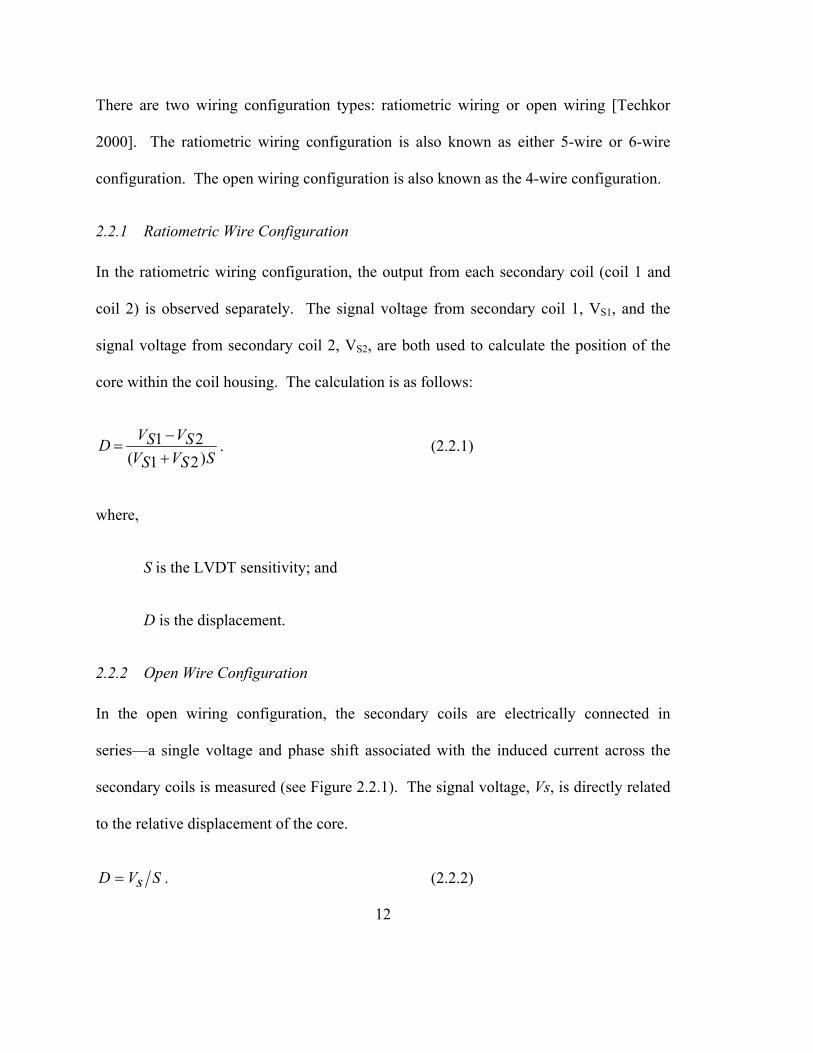
LVDT. Figure 2.2.2 shows the data of an LVDT with a 61 m cable length before and
after applying the SCF. The factory supplied sensitivity was 396 mV/V/0.001 in. Figure
2.2.2 shows a slope (SCF) of 1.082 for the factory sensitivity based data. Multiplying the
slope by the factory sensitivity, and rounding to the nearest whole number, a sensitivity
of 428 mV/V/0.001 in was used to acquire a new data set. A slope of 1.0009 was
obtained as shown in the sensitivity correction plot in the figure. This was repeated for
seven lengths of cable ranging from 49 m to 73 m at 4 m intervals—this covered the full
range of cable length used during a monitoring program.
During this process, a linear relationship between the adjusted sensitivity and cable
length was observed for that range. Figure 2.2.3 is a plot of a sensitivity correction factor
(SCF) versus cable length, l, in meters. A trendline was plotted. The linear regression
of the SCF data produces an R2 value of 0.9867. The result of the linear regression is the
following equation of the SCF in terms of cable length:
)(0013.01)( λλ +=SCF . (2.2.3)
15

61 m Long Cable LVDT vs. Calibration LVDT
Sensitivity Correction = 428y = 1.0009x - 1.0846
R2 = 0.9998
Factory Sensitivity = 396y = 1.082x - 1.1725
R2 = 0.9998
0
0.5
1
1.5
2
2.5
1 1.5 2 2.5 3 3Calibrated LVDT Position (inches)
Cab
led
LVD
T P
ositi
on (i
nche
s)
.5
Figure 2.2.2. Effect of Sensitivity Correction Factor (SCF).
Sensitivity Correction Factor (SCF)
SCF = 0.0013(l) + 1
1.00
1.02
1.04
1.06
1.08
1.10
1.12
0 10 20 30 40 50 60 70 8Cable Extension Length [l] (m)
SC
F
0
SCF based on Factory Sensitivity
SCF Used for Cable Length Adjustment
Figure 2.2.3. LVDT Sensitivity Correction Factor vs. Cable Length. 16

17
The author determined that multiplying the manufacturer’s provided sensitivity by the
SCF is a good adjustment to the sensitivity for the combination of cables and LVDTs
used. Without the SCF adjustment, as applied to this application, the LVDT would
indicate a 10% larger deflection than exists for a cable length of 75 m, as shown in Figure
2.2.3. Information such as this is not typically provided by the LVDT manufacturer or by
the signal conditioner manufacturer. The documentation for the signal conditioner used
during this research did state that cable lengths of greater than 100 meters could cause
significant errors [NI 2000, pg 2-4]. This is just one example of a technique to determine
the appropriate sensitivities for the field condition. The resulting relationship is not
necessarily appropriate for any LVDT setup with long cables—the technique, however, is
portable. Since every different specified cable has different impedance properties, this
process should be repeated for each type of cable used.
2.2.5 Limitations for Structural Health Monitoring
The primary limitation of the LVDT is the establishment of a baseline to measure against.
Typically, in the laboratory, there is a location adjacent to the structural element of
interest that is not a part of the load path nor affected by the testing protocol. LVDTs can
be used in bridges and buildings to measure relative movements, such as: displacements
across expansion joints, thermal extension between two points along the length of a
member, the diagonal racking displacement of a plywood shear wall, et cetera. To
observe beam deflection, an available technique is the taut wire baseline system which is
discussed in detail in Chapter 3.

18
2.3 Strain Gauges
A strain gauge is composed of a material with a measurable property sensitive to its own
change in length. When the relationship between the measurable property and strain can
be established, a material can be used as an effective strain gauge. There are many
different types of strain gauges. The material of the structure studied, the full scale
magnitude of expected strain, the required frequency of strain measurements, and the
surrounding environmental conditions will determine what type of strain gauge is best
suited for the application. As opposed to using strain gauges in a laboratory, in structural
health monitoring, strain gauge thermal output must be considered a significant potential
source of error. Without properly considering the thermal output of strain gauges at the
beginning of a structural health monitoring program, it can be difficult to isolate
mechanical behavior based on direct strain readings alone. This section will describe:
three types of strain gauges; some thermal effects to consider during a SHM program;
and a comparison of the discussed strain gauges.
2.3.1 Types of Strain Gauges
In this section, three types of strain gauges are discussed: electrical resistance strain
gauges, fiber optic strain gauges, and vibrating wire strain gauges. It should be noted,
strain can also be observed by devices that are designed to measure relative displacement
between two discrete points. The strain is calculated as the relative displacement of the
device divided by the initial distance between the discrete points. This type of strain
determination will not be discussed in this section.

2.3.1.1 Electrical Resistance Strain Gauges
Electrical resistance strain gauge technology is well established and widely used. The
material property of electrical resistance is sensitive to the mechanical change in length
of some conductors. These conductive materials, typically metals or metal alloys, exhibit
sensitivities that are linearly related to strain. The measurements can be significantly
impacted by electrical connection changes in the system. Also, the sensitivity is
influenced by temperature.
2.3.1.1.1 Basics of Observing Resistance Change
Directly observing the change in resistance with an ohmmeter is not generally accurate
enough for currently available strain gauges. Instead we use Ohm’s Law—voltage, V,
equals the product of current, I, and resistance, R:
IRV = . (2.3.1)
A voltage divider circuit is the simplest way to measure a change in resistance (see
Figure 2.3.1). A voltage divider circuit is powered by a constant supply voltage, Vex,
while a signal voltage, Vs, changes with the resistance of resistors R1 and/or R2. In
Figure 2.3.1, Vs is measured across resistor R2, and Vex is applied across both resistors R1
and R2. By Ohm’s Law and the summation of resistance: Vex = I (R1 + R2), where I is the
current flowing through the resistors R1 and R2.
19

Figure 2.3.1. Voltage Divider Circuit.
Currently available strain gauges have resistances of 120, 350, and 1000 ohms. The
sensitivity of each gauge is expressed as a gauge factor, GF. The gauge factor is a ratio
between the relative change in resistance and strain:
εRdRGF = . (2.3.2)
Metallic foil strain gauges have gauge factors that are typically between 1.90 and 2.10.
Consider the voltage divider circuit in Figure 2.3.1, let R1 be a 350 ohm resistor and R2
be a 350 ohm strain gauge with GF = 2.00. If Vex = 7.000 V, the current, I, by equation
(2.3.2) is 10 mA. The initial unstrained signal voltage across R2 is Vs = I (R2) = 3.500 V.
As seen in the sample calculations in Figure 2.3.2, a 5 microstrain change in the strain
gauge will result in a resistance change of 0.0035 ohms or a 0.035 mV change in the
signal voltage. 20

21
dR/R = GF(ε). => dR = GF (ε) R.
Let: ε = 5µε; R = 350 ohms; GF = 2.0; I = Vex/Rtotal = 10 mA.
dV = I dR = I GF (ε) R = 10 mA (2.0) (0.000005 in/in) 350 ohms.
dV = I dR = 10 mA (0.0035 ohms) = 0.035 mV.
Figure 2.3.2. Sample Calculation to Find Voltage Resolution (5µε measurement).
The strain resolution will depend on the smallest increment of measurement of the
voltmeter—a smaller measurable voltage leads to a better strain resolution. A better
strain resolution can also be achieved by increasing the excitation voltage. This can be
shown by repeating the sample calculation shown in Figure 2.3.2 with a larger excitation
voltage, Vex. An increased current through the strain gauge resistor will magnify the
signal voltage, Vs, for a set change in strain. However, there is a practical limit to
increasing the current which must be considered (see section 2.3.3.1 for more detail).
2.3.1.1.2 Wheatstone Bridge Based Strain Measurements
Temperature changes in the strain gauges and in the long cable leads between the data
acquisition system and electrical resistance strain gauges can cause spurious indicated
strain readings. To compensate for this occurrence, a common approach is to create an
electrical compensating network [Fraden 2004, pg 326]—the Wheatstone bridge is one
type.

22
As described in the previous section 2.3.1.1.1, a voltage divider is constructed using two
resistors in series. The circuit is completed by applying an excitation voltage across the
series. The voltage measured at the node between the two resistors is a fraction of the
excitation voltage as determined by Ohm’s law and Kirchhoff’s rules. Using a strain
gauge as one of the resistors causes the measured voltage to change with strain.
Similarly, a Wheatstone bridge provides a way to measure voltage to indicate strain. The
bridge circuit is two voltage divider circuits in parallel—both voltage divider circuits are
powered by the same excitation voltage source. The signal voltage is then measured
between the two voltage divider output nodes. This circuit is the standard circuit used
with electrical resistance strain gauges. It can be used to improve performance and
provide application adaptability of strain gauge based measurements. The bridge circuit
can increase the resolution of strain measurements and perform temperature
compensation. Chapter 4 describes two applications for measuring a crack mouth
opening displacement and the rotation at a pinned connection using devices built with
electrical resistance strain gauges.
Shown in Figure 2.3.3, the resistors R1 and R3 form a voltage divider circuit; and resistors
R2 and R4 form the other. The voltage divider outputs are at nodes b and c, respectively.
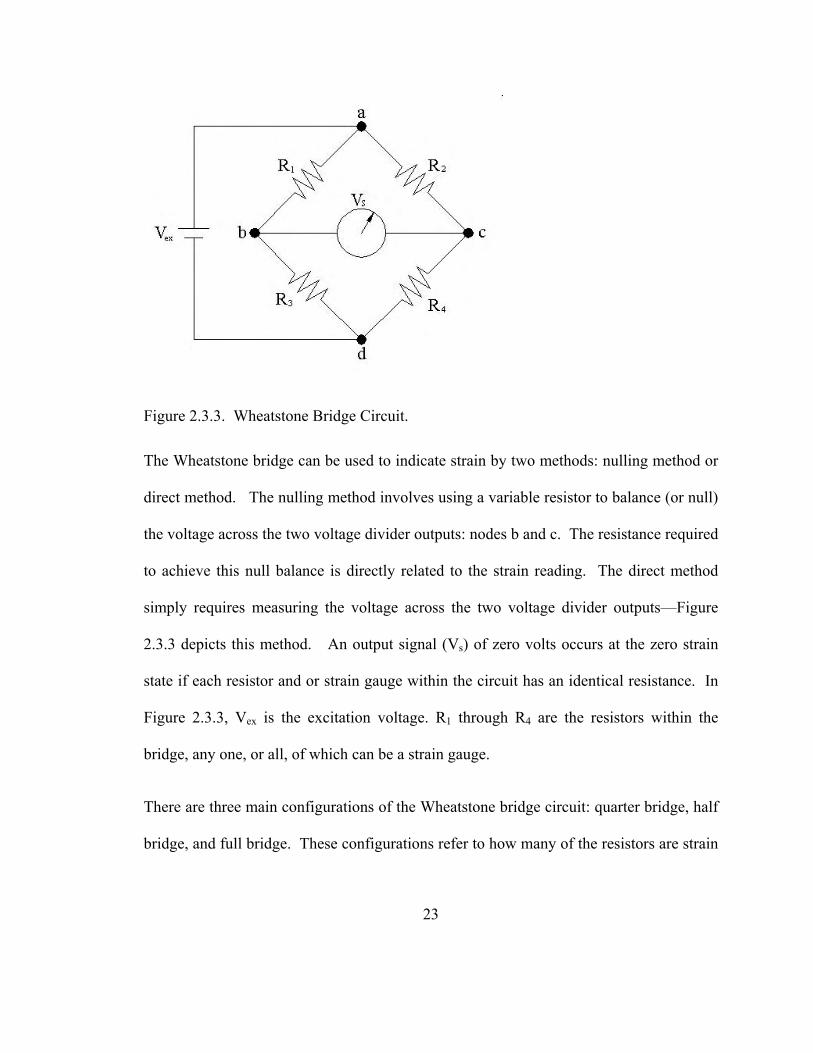
Figure 2.3.3. Wheatstone Bridge Circuit.
The Wheatstone bridge can be used to indicate strain by two methods: nulling method or
direct method. The nulling method involves using a variable resistor to balance (or null)
the voltage across the two voltage divider outputs: nodes b and c. The resistance required
to achieve this null balance is directly related to the strain reading. The direct method
simply requires measuring the voltage across the two voltage divider outputs—Figure
2.3.3 depicts this method. An output signal (Vs) of zero volts occurs at the zero strain
state if each resistor and or strain gauge within the circuit has an identical resistance. In
Figure 2.3.3, Vex is the excitation voltage. R1 through R4 are the resistors within the
bridge, any one, or all, of which can be a strain gauge.
There are three main configurations of the Wheatstone bridge circuit: quarter bridge, half
bridge, and full bridge. These configurations refer to how many of the resistors are strain
23

24
gauges. Logically, a quarter bridge uses only one strain gauge out of four resistors, a half
bridge uses two strain gauges, and a full bridge four strain gauges.
For a single strain gauge, the quarter bridge is typically used. This configuration is
susceptible to the thermal output of the strain gauge. Also, this signal conditioning
network is usually physically separated. The strain gauge is attached to the specimen and
the other three resistors are within the data acquisition hardware. Long electrical leads
will act as an antenna picking up electrical noise and changing resistance with
temperature along their length. To account for these error-inducing impedances, the lead
length effect is introduced to both sides of the bridge circuit—both voltage dividers. This
is done by using three lead wires for the strain gauge—schematically shown in Figure
2.3.4. The signal voltage, Vs, will not change with a common equal resistance change
along b-d, and c-d. A small resistance change RL between node d and the excitation
source, will not significantly change Vs either.

Figure 2.3.4. Long Lead Quarter Bridge Configuration.
The half bridge configuration utilizes both voltage divider circuits to perform one of the
following: amplify the signal voltage; perform strain gauge thermal output compensation.
For a half bridge configuration, typically, resistors R1 and R2, or R3 and R4, are the active
strain gauges. Signal amplification is achieved by using two strain gauges which are
mounted in such a way that one experiences positive strain while the other experiences
negative strain. As an example, if one gauge is applied perpendicular to the other, strain
applied in one direction will cause a negative strain in the other, due to Poisson’s effect.
This produces a greater signal voltage than one gauge alone: both voltage dividers are
affected in opposing directions. The thermal output of both gauges will be identical and
are already applied to both sides of the bridge—temperature compensation is automatic.
If thermal output compensation is required, without signal amplification, one gauge
(called a “dummy” gauge) can be mounted on similar material that is only exposed to the
temperature changes and not the mechanical loading. Thermal output compensation
25

26
achieved in a half-bridge configuration can be done in such a way that adjusts for lead
length. The quarter bridge configuration does not perform strain gauge thermal output
compensation.
The full bridge configuration, like the half bridge, can compensate for strain gauge
thermal output and can amplify the signal voltage by up to four times that of the quarter
bridge. This configuration is commonly used for making load cells, extensometers, and a
variety of other devices. Chapter 4 shows the use of the full bridge configuration to
measure crack mouth opening displacements and rotational displacements at a bridge
pinned support.
2.3.1.1.3 Thermal effects
Generally, the sensitivity as a function of temperature is non-linear. The temperature
sensitivity of electrical resistance strain gauges can be compensated for in a variety of
ways. There is no one best way; it all depends on the application. For structural health
monitoring applications, there are two sources where temperature induced systematic
error can occur: the effect of temperature change on the long cable leads between the data
acquisition system and the strain gauge, and the effect of temperature change on the
strain gauge itself.
The temperature change on long cable leads for a single strain gauge is easily handled.
The Wheatstone bridge in a quarter bridge configuration is utilized. The specific wiring
requirement to achieve this is shown in Figure 2.3.4 and discussed in section 2.3.1.1.2.
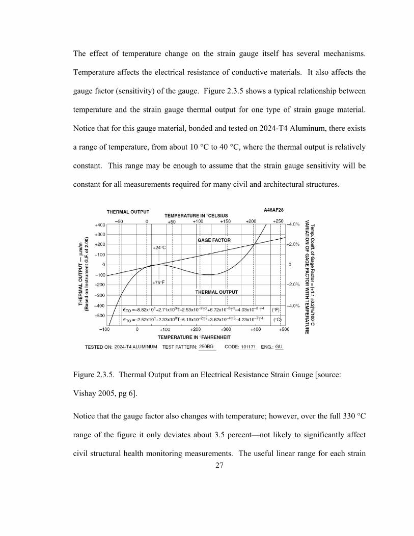
The effect of temperature change on the strain gauge itself has several mechanisms.
Temperature affects the electrical resistance of conductive materials. It also affects the
gauge factor (sensitivity) of the gauge. Figure 2.3.5 shows a typical relationship between
temperature and the strain gauge thermal output for one type of strain gauge material.
Notice that for this gauge material, bonded and tested on 2024-T4 Aluminum, there exists
a range of temperature, from about 10 °C to 40 °C, where the thermal output is relatively
constant. This range may be enough to assume that the strain gauge sensitivity will be
constant for all measurements required for many civil and architectural structures.
Figure 2.3.5. Thermal Output from an Electrical Resistance Strain Gauge [source:
Vishay 2005, pg 6].
Notice that the gauge factor also changes with temperature; however, over the full 330 °C
range of the figure it only deviates about 3.5 percent—not likely to significantly affect
civil structural health monitoring measurements. The useful linear range for each strain 27

28
gauge material should be considered when selecting a gauge for a particular application.
If the non-linear range is needed, temperature compensation is suggested (see section
2.3.2).
2.3.1.2 Fiber Optic Strain Gauges
Fiber optics technology is relatively new; however, it has rapidly become the standard for
high speed communications equipment. This technology is capable of transmitting vastly
greater amounts of data than its electronic copper wire predecessor. Fiber optic cable is
composed of two layers of glass, or plastic polymer. The inner layer is called the core.
The outer layer is called the cladding. Light is transmitted through the core by utilizing
the phenomena of total internal reflection. This phenomenon is possible because the
cladding has a lower index of refraction than the core. The cladding acts as a waveguide
which helps to maintain signal intensity. Light enters the core at a polished end of a
cable. As the light’s angle of entry, into the core, tends toward normal, the light will tend
to be reflected off the cladding back into, and propagate through, the core [Fraden 2004].
The light can be transmitted through fiber optic cables with much less energy attenuation
than electricity through copper cable—subject to electrical resistance. Light also has a
broader signal spectrum that can be utilized for transmitting data. The light signal is
unaffected by a magnetic field-filled environment—passing vehicles, power lines, et
cetera. The properties of light also allow for transmitting data in both directions on the
same fiber. Fiber optic strain gauges are designed such that as the gage length of the
fiber is strained, the reflective properties within the fiber core also change. This effects a

change to both the light signals reflected off, and transmitted through, the gauge. Two
common approaches to making the core sensitive to strain and measuring its effects upon
the reflected light are discussed here: Fabry-Perot interferometry and Bragg grating
modulation.
2.3.1.2.1 Fabry-Perot Based Strain Gauges
Fabry-Perot interferometer based strain gauges relate strain to the reflection of light
across a cavity between two polished partially silvered optical fibers, as seen in Figure
2.3.6. The cavity and partially reflective surfaces form a Fabry-Perot etalon, Figure 2.3.7.
The purpose of this etalon is to create, and simultaneously transmit/reflect, multiple
parallel rays of light. The new light signal will consist of a spectrum of light with some
wavelengths in which constructive interference will occur and other wavelengths in
which destructive interference will occur. The ray shown propagating across Figure 2.3.7
is that of a ray at a constructive wavelength: upon passing through the focusing lens, the
rays’ intensities combine on the screen. The constructive and destructive interference is
dependent on the length of the Fabry-Perot cavity. By observing the change in the
wavelengths where the maximum constructive interference occurs, the change in length
of the Fabry-Perot cavity can be determined.
29 Figure 2.3.6. Fabry-Perot Fiber Optic Strain Gauge [source: Fiso 2006].

Figure 2.3.7. Fabry-Perot Etalon [source: Drexel 2006].
2.3.1.2.2 Fiber Bragg Grating Based Strain Gauges
Bragg grating modulation based strain gauges measure either the reflection or
transmission of a specific wavelength of light. To make this type of gauge, the fiber optic
core of a fiber is irradiated with ultraviolet light. The fiber core is photosensitive. At the
location of the irradiation, periodic alterations of the core’s refractive index—Bragg
gratings—are created. The core alterations are burned into a single mode optical fiber at
a period, Λ, selected for the gauge, where:
λ = 2 neff Λ. (2.3.3)
The period of the grating, Λ, and the effective modal refractive index, neff, determine the
Bragg grating wavelength, λ. As Figure 2.3.8 shows, the Bragg grating wavelength of
light is reflected and does not transmit with high intensity beyond the irradiated core
location. Stretching the fiber at the location of the grating changes the reflected
wavelength. This change in wavelength is directly related to the strain in the fiber.
30
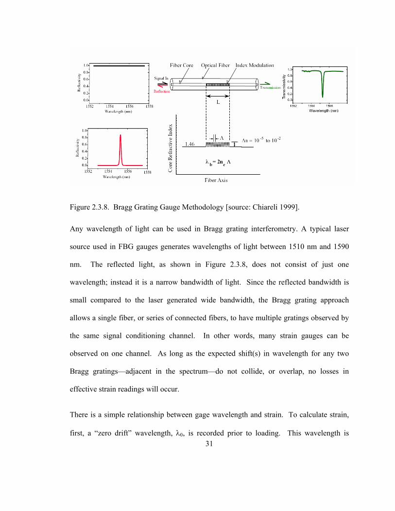
Figure 2.3.8. Bragg Grating Gauge Methodology [source: Chiareli 1999].
Any wavelength of light can be used in Bragg grating interferometry. A typical laser
source used in FBG gauges generates wavelengths of light between 1510 nm and 1590
nm. The reflected light, as shown in Figure 2.3.8, does not consist of just one
wavelength; instead it is a narrow bandwidth of light. Since the reflected bandwidth is
small compared to the laser generated wide bandwidth, the Bragg grating approach
allows a single fiber, or series of connected fibers, to have multiple gratings observed by
the same signal conditioning channel. In other words, many strain gauges can be
observed on one channel. As long as the expected shift(s) in wavelength for any two
Bragg gratings—adjacent in the spectrum—do not collide, or overlap, no losses in
effective strain readings will occur.
There is a simple relationship between gage wavelength and strain. To calculate strain,
first, a “zero drift” wavelength, λ0, is recorded prior to loading. This wavelength is 31

analogous to an initial specimen length, Li. Any observed wavelength during loading, λ,
is analogous to the new length of the strained specimen, Ls. Assuming that only the
grating pitch is affected by fiber extension or compression, to calculate strain, simply
apply the analogous quantities to the definition of strain,
0
0λ
λλε
−=
∆=
−=
iLL
iLiLsL . (2.3.4)
The assumption that fiber strain only affects the grating pitch is incorrect. Fiber strain
also affects the effective modal index, neff. As a structural engineer might imagine, the
modal index can be affected by Poisson’s ratio and transverse loading affecting a variety
of optical/reflective implications within the fiber. Others have shown or observed, for the
case of a homogeneous, isotropic axial straining of a Bragg grating, the relationship
between strain and wavelength shift—including changes in neff—is approximated as
shown in equation (2.3.3) [Meltz 1996, pg4]:
ελλ
λ
λλ78.0
0
0 ≈∆
=−
. (2.3.5)
To further illustrate this relationship; let us determine the required wavelength measuring
resolution to obtain a 1 microstrain observation resolution. It is obvious that the shorter
“zero drift” wavelength will experience a smaller wavelength deflection for the same
value of strain—a shorter gauge length sees a smaller deflection. Since the range of
available wavelengths is from 1510 nanometers to 1590 nanometers, choose the smallest
32

33
possible “zero drift” wavelength of λ0 = 1510 nanometers and solve equation (2.3.5) for
∆λ, where ε = 1 µε = 10-6 in/in (mm/mm):
∆λ ≈ 0.78 * 10-6 (1510 nm) = 1.178 picometers.
This can also be written as a sensitivity of the gauge, 1 µε /1.178 pm, or 0.8490 µε /pm.
The sensitivity of a gauge at the opposite end of the spectrum is 1 µε /1.240 pm, or
0.8063 µε /pm.
The initial, “zero drift” wavelength should not be confused with the gauge length of the
strain gauge. For this type of strain gauge, the gauge length can be flexible. If the fiber
is directly, or continuously, bonded to the specimen, it is probably safe to assume the
gauge length is the length over which the core alterations are manufactured. If the fiber
is maintained taut between two points attached to the specimen, the gauge length is the
distance between those two points—even if the gratings only occur over a shorter
distance. It should be noted that if part of the FBG is strained more than another, the
reflected wavelength spectrum will be broader than the initial reflected wavelength
[Wnuk 2005].

Figure 2.3.9. Reflected Spectrum Changes due to Residual Strains [source: Wnuk 2005,
pg 5].
The methodology of gauge attachment dictates actual strain observation. The curing of
the epoxy may cause residual strains to occur at the Bragg grating locations. Observation
of this behavior during installation is necessary such that the true "zero drift" reading is
known. Care should be taken to understand the method by which the data acquisition
interrogator determines the reflected wavelength. The broadening of the reflected
spectrum—shown in Figure 2.3.9 by the difference in mounted and unmounted pattern—
may cause different effects on the acquisition of the light signal. This could take the
form of multiple “detected” wavelengths (multiple peak intensities), or a less stable
detected wavelength. This effect may vary on different signal conditioning products
34

since this technology is still in the product development stage and has not arrived at a
standard “best” method yet.
2.3.1.3 Vibrating Wire Strain Gauges
Vibrating wire strain gauge technology is widely used and well established. The
vibrating wire strain gauges operate on the principle of resonance. These gauges operate
by magnetically plucking a tensioned wire and measuring its free vibration response. The
wire is pre-tensioned across the length of the gauge; as the gauge is stretched the tension
in the wire changes and its resonant frequency changes. The resonant frequency is a
function of both strain and the ambient temperature. Equation (2.3.6) expresses that
function in terms of the mechanical properties of the wire. Equation (2.3.7) is the
temperature-compensated strain as a function of the measured frequency and
temperature.
TmL
EA
mL
EAf ∆−= 24242 αε . (2.3.6)
TfEAmL
∆+= αε 224 . (2.3.7)
For equations (2.3.6) and (2.3.7): f is the resonant frequency of the wire; L is its length; m
is the mass per unit length; E is the elastic modulus; A is the cross-sectional area; α is the
coefficient of thermal expansion; ∆T is the change in temperature from the initial
temperature.
35

36
Vibrating wire strain gauges are very stable strain gauges. These gauges can be
embedded or surface mounted. The thermal output, in terms of the change of resonant
frequency, is easily compensated. However, because the wire needs to be plucked each
time a reading is taken, the minimum recording period is approximately one second. This
does not allow for observation of dynamic events.
2.3.2 Thermal Effects and Considerations for Strain Gauges
For structural health monitoring applications, there are two primary sources where
temperature induced systematic error can occur: the effect of temperature change on the
strain gauge material itself, and the effect of thermal expansion interactions between the
gauge and attached material. Generally, the first source relates to the gauge sensitivity as
a function of temperature. This is commonly non-linear over a broad range of
temperatures. However, it can be represented as a linear function within a used range
that is narrow. In any range of use, the thermal sensitivity/output should be identified for
variable temperature environments—usually affecting structural health monitoring
applications.
The second source can promulgate false strain readings when the strain gauge and test
specimen material have differing coefficients of thermal expansion. Temperature affects
the physical behavior of both the strain gauge and the material to which it is adhered.
Any change in temperature of a material causes thermal straining of that material.
Usually, the thermal strain, εt, is directly related to the temperature change, ∆T. This
linear relationship is described by the coefficient of thermal expansion, α, where

37
εt = α ∆T. (2.3.8)
If the mechanical loading of a structure is to be considered alone, and it is tested in a
constant temperature environment, any difference in α between the strain gauge and the
material being strained would not affect the indicated strain. However, identical
coefficients of thermal expansion are desirable if a structure is being tested in an
environment with varying temperature. Differing thermal expansion of the strain gauge
and the specimen will cause an apparent strain. The stiffness of the specimen, by design,
is much greater than that of the gauge. A strain gauge will be restrained by the specimen
stiffness such that the gauge’s thermal expansion will create an apparent strain that is
only internal to the gauge material. This effect can and should be calibrated to the
specimen thermal material properties. The indicated strain would be the sum of the real
strain of the specimen and the apparent strain [Norton 1989]. The terms apparent strain,
indicated strain and real strain are nicely defined in chapter 9.5 of “Handbook of
Transducers” [Norton 1989].
For each strain gauge technology, both gauge sensitivity and apparent strain effects will
be handled in different ways. As a general analytical tool, the measurable phenomenon
observed by each technology can be described as a function of mechanical strain and
temperature change.
∆P/P = Sε ε + ST T (2.3.9)

38
∆P is the change in the measurable phenomenon. P is the initial phenomenon
measurement. Sε is the mechanical strain sensitivity of the gauge. ε is the mechanical
strain in the specimen. ST is the thermal expansion sensitivity of the gauge—or the gauge
restrained by the specimen—some gauges are calibrated on a particular material, say
1018 steel [Vishay 2005].
Table 2.1 shows the different parameters, as applied to equation (2.3.9) for some strain
gauge technology types. The first column lists the strain gauge technology type. The
second column is the measurable phenomenon. The third column lists the expression that
describes the mechanical strain sensitivity. The fourth column lists the expression that
describes the thermal expansion sensitivity.
Table 2.1. Strain Gauge Behavior Sensitivities.
Strain Gauge Technology
Phenomenon Measured
(P)
Mechanical Strain Sensitivity Expression
(Sε ε)
Thermal Expansion Sensitivity Expression
(ST T)
Electrical Resistance Foil
(ERSG) ∆R/R GF ε εto(T)
Fabry Perot Fiberoptic
(FPSG) ∆Lcavity Lgε βLgε
Fiber Bragg Grating Fiberoptic
(FBGSG) ∆λ/λ0 (1-Pe) ε Z ∆T
Vibrating Wire
(VWSG) f2 EA/(4mL2) ε α EA/(4mL2) ∆T

39
As an illustration, for electrical resistance strain gauges (row one of Table 2.1) the full
indicated output, equation (2.3.9), can be described by the following equation:
∆R/R = GF ε + εto(T). (2.3.10)
R is resistance in ohms; GF is called the gauge factor, usually between 1.90 and 2.10.
The GF is also a function of temperature but has a much less significant impact than the
εto(T) function—described further in Vishay [Vishay 2005, pg 6]. In this case, the
thermal output of the strain gauge, εto, is a non-linear function of T which is provided by
the manufacturer. An example function from Vishay Micro-Measurements is as follows:
εto(T) = -73.7 + 5.10 (T) – 9.17(10)-2 (T2) + 4.48(10)-4 (T3) – 5.50(10)-7 (T4)
T has the units of °C. εto has units of microstrain.
These relationships should help an investigator to determine the best course of action to
account for thermal loading of the structure and attached instrumentation.
2.3.2.1 Thermal Output Compensation Techniques
The relationships generally described by equation (2.3.9) and Table 2.1 above help the
investigator to understand the potential effect of temperature and mechanical deformation
on indicated strain. The strain indicated by a data acquisition device directly from the
measured phenomena is not segregated into thermal and mechanical components. Signal
conditioning per each respective strain gauge technology can help to do this. It is usually
done through the use of a signal conditioning network [Fraden 2004, pg 195]. However,

40
this type of compensation is discussed in other sections. Aside from signal conditioning
networks, the calculation of real strain can be handled in other ways based on the
principles of the constitutive relationships described in Table 2.1. The problem addressed
here is the measured strain value is inseparable from the sum of the mechanical and
thermal effects. This section describes temperature compensation as a function of the
thermal output of a strain gauge, specifically two techniques: (1) using a baseline of
indicated strain, due to diurnal temperature effects, observed on the test specimen; and
(2) using a second temperature observation applied to a formula based compensation
routine.
2.3.2.1.1 Thermal Baseline Measurements Technique
The first technique involves installing the strain gauges onto the test specimen and
observing the change with temperature over a period of time to establish a baseline. If a
continuous structural health monitoring program is planned this is easily incorporated.
As an illustration, Figure 2.3.10 shows typical data that is collected during one day of a
bridge structure. As one can see, even without an in-depth analysis, for structures such as
bridges, traffic loading or earthquake loading measurements are quite identifiable even
with the thermal loading superimposed onto it. The mechanical loading happens much
quicker than the thermal loading. The measurements just prior to the mechanical loading
event can be considered the zero baselines and will provide sufficient “temperature
compensated” results.

Figure 2.3.10. Typical Structural Diurnal Response.
To apply this idea to an automated SHM system, more sophistication is required but this
technique can still be reasonably applied. It can be done by calibrating a thermal
compensation algorithm with data from an initial short-term study at the start of a project.
This algorithm can apply a compensating calculation to future data based on the initial
temperature dataset. This refinement could be utilized to help isolate the mechanical
strain behavior of interest to the structural engineer.
During the initial study period, thermal fluctuations representative of the expected
temperature range through the course of the project should be used. This becomes more
important when the type of gauge has a non-linear thermal output over the expected
range—this is not common for civil or architectural structures, but should be considered
as new technologies are evaluated.
41

42
More research needs to be done to see if periodic “thermal cycle” testing, during the
course of an instrumentation project, can provide relevant information about systematic
mechanical deterioration. A change in the temperature / indicated strain relationship has
the potential to identify the change in mechanical properties such as flexural rigidity. To
illustrate this point, if a reinforced concrete beam’s effective flexural rigidity was
determined to be 50% of the gross section during a load test, and the thermal deflection
behavior was also observed, any deviation from subsequent thermal behavior could
indicate deterioration of the flexural rigidity as a result of crack growth or increased
number of cracks. This has not yet been tested, but there is potential.
2.3.2.1.2 Calculated Apparent Strain Removal Technique
The second method to extract the real mechanical strain from a temperature influenced
indicated strain is to measure the temperature. This can be done either directly or by use
of a “dummy” gauge isolated from the mechanical loading of the test structure. Applying
those measurements to the associated compensation formulas, characterized by Table 2.1,
allow identification of the apparent strain. In this approach, the temperature will
determine the apparent strain that needs to be removed from the indicated strain to obtain
the real mechanical strain.
As an example, fiber Bragg gratings have a typical temperature sensitivity of 10 pm/°C
near a wavelength of 1550 nm [Meltz 1996, pg 4]. Following the wavelength to strain
conversion methodology in section 2.3.1.2.2, the strain thermal sensitivity is
1µε/(0.78*1.55pm) * 10 pm/°C, or 8.27 µε/°C. This is also known as the gauges

43
coefficient of thermal expansion, αG. Concrete’s α value is typically between 8 and 12
µε/°C. Steel’s α value is typically between 11 and 12 µε/°C. Any difference in α
between the gauge and the material can cause a spurious "apparent strain" to be observed
[Norton 1989, pg 184].
When a strain gauge is used in a temperature-controlled environment, with a constant
temperature, the “apparent strain” will be constant for all readings and is automatically
removed when comparing two strain readings. However, when the temperature is
variable, the “apparent strain” is not constant. This spurious strain can be removed with
the use of an additional temperature compensation gauge. A temperature compensation
gauge should be mounted, such that it is unaffected by the mechanical loading of the
observed specimen. It should also be designed such that it correctly reflects the boundary
conditions—restraint—of the other strain gauges measuring mechanical strain. For
example, if a strain gauge is attached to the structure at only two points—as some gauges
are designed—and is unbonded along the length of the gauge, the temperature
compensation gauge should also be unbonded along its length. In this way, the α of both
strain gauges is matched; a direct subtraction of the mechanically free strain gauge
reading from the mechanically sensitive strain gauge reading eliminates the “apparent
strain” from the signal acquired during the observation of the structure.
Figure 2.3.11 shows the output of a type of strain gauge that has a coefficient of thermal
expansion of 30 µε/°F when mounted on two different materials. The plot labeled “A”
results when the gauge is bonded to a steel specimen (α = 6.7 µε/°F). The plot labeled

“B” is what the manufacturer of the gauge describes as the estimated result if the same
gauge was installed on a material with α = 35 µε/°F [Vishay 2005].
Figure 2.3.11. Strain Gauge Output Change Due to α Mismatch Effects [source: Vishay
2005, pg 9].
If the α of the gauge and the material to which it is bonded match, the indicated strain as
a function of temperature would produce a flat line on the graph. The slopes of the plots
in Figure 2.3.11 represent a difference in α between the material and the gauge. A
negative indicated strain, mechanically analogous to compression, for an increase in
temperature is the result of α being larger for the gauge than for the specimen. A
negative slope in Figure 2.3.11 is consistent with this type of gauge and specimen
interaction. A positive slope is consistent with the inverse behavior.
44

Equation (2.3.11) is a simplified thermal output formula that can be used to help
compensate for the apparent strain experienced by electrical resistance strain gauges
[Vishay 2005, pg 8]. It provides a way to estimate the change in thermal output of a
gauge that is bonded on a material that is different from the material on which it is
calibrated.
TSTGGFG
T ∆+∆⎟⎟⎠
⎞⎜⎜⎝
⎛−= αα
βε . (2.3.11)
The process to obtain the estimate involves utilizing the difference between two iterations
of this equation [Vishay 2005]. We consider both iterations for the same gauge type so
the first term in the equation cancels (variables within the parenthesis are identical).
What remains is an equation that states that the difference in thermal output, εT, due to
the difference in the α values of two substrates:
TSSSTST ∆−=− )21
()2()1( ααεε . (2.3.12)
This information and technique can be applied to determine the thermal output of a strain
gauge on a substance with a different coefficient of thermal expansion, α; it can be
applied to determine the α of the test specimen; and to determine the effective coefficient
of thermal expansion, αeff, of other strain gauges for narrow ranges of temperature—such
as with civil SHM. By using this technique with additional strain gauges that are only
affected by temperature changes of the substrate material, the real mechanical strain can
be retrieved from the indicated strain.
45

46
2.3.3 Structural Health Monitoring Strain Gauge Comparison
Each type of strain gauge has advantages and disadvantages depending on the phenomena
of interest in an investigation. Civil engineering structural materials have varying
mechanical properties that affect which strain gauge type should be used.
Concrete, steel, wood, aluminum, fiber reinforced plastic, and other materials will each
have similar but distinct issues that need to be addressed. Some questions that need to be
considered when observing the behavior of concrete or reinforced concrete structures
include: Will cracking behavior occur? What gauge length is appropriate to measure the
phenomena? Will the assumption that the concrete is homogenous be appropriate? Will
aggregate shape, size and location potentially affect the results? Will the strain be
monitored on a short-term or a long-term time scale? What type of surface preparation is
required for adhesion of the gauge? Will temperature be stable or variable? This section
will not attempt to answer all these questions, instead, it will help the investigator to
make their own decision based on some of the identified advantages and disadvantages of
each discussed strain gauge type.
2.3.3.1 Electrical Resistance Strain Gauges
As shown by the sample calculation in Figure 2.3.2, a typical strain change, of interest to
engineers, causes a very small change in resistance and in turn measured voltage. This
has several significant consequences. First, as mentioned earlier, an ohmmeter does not
provide an adequate resolution for direct measurement of strain. Second, in terms of
portability of a structural health monitoring system, the strain gauge leads cannot be

47
disconnected from the system without loss of the initial reading. This is limiting such
that once the strain gauges are installed, they must be left installed to acquire long-term
measurements—no disconnecting and reconnecting the data acquisition system. Third,
special care must be taken to protect the electrical leads from corrosion and other similar
physical damage that may alter the resistance within the measurement circuit.
Additionally, the user should be aware that both resistors and electrical resistance strain
gauges cannot tolerate an infinite range of current. Indeed, the maximum applied current,
or guidance on how to determine such [Vishay 2005], is usually reported by the
manufacturer of the strain gauge. Also, the smallest measurable voltage is usually
reported by the manufacturer of the signal conditioner. Lastly, although the signal from
an ERSG is analog, digitization for storage can limit either the resolution or dynamic
range of the signal. Any one of these may limit the usefulness of the data acquisition
system for the electrical resistance strain gauges.
2.3.3.2 Fiber Optic Strain Gauges
Fiber optic strain gauge technology is still in the development phase. The two
technologies discussed in this chapter—Fabry-Perot and Bragg grating—have both been
developed to the point where they can be used in structural health monitoring projects.
However, there are not many producers of quality gauges that have withstood the test of
time. Product development on both the gauge design side and the signal conditioning
side continues.

48
Fabry-Perot gauges and Bragg grating gauges are competing for which provides the best
product. An earlier advantage of Fabry-Perot gauges having a better resolution of strain
must be weighed against the Bragg grating’s ease of multiple sensors on a single
fiber/signal conditioning channel.
Some of the primary advantages for using fiber optic strain gauges include: a stable
reading that can be disconnected and reconnected without loss of the initial measurement;
the ability to acquire high frequency data—up to 250 Hz; newer models are advertised to
1000 Hz; and resistance to electromagnetic radiation from power lines, larger vehicles,
and broadcast stations.
At this time, it is this author’s opinion that Bragg gratings are more easily and cheaply
incorporated into a structural health monitoring program. However, current research
continues in its search to perfect designs of both these technologies [Ferreira et al. 2000,
Henriksson et al. 1996, Zhu et al. 2003, Lopez-Higuera 2005, etc.] as well as to develop
other methodologies to observe strain. A new gauge being developed / tested is a
highbred extrinsic Fabry-Perot interferometric/in-fiber Bragg grating gauge; the gauge
simultaneously measures strain and temperature [Rao et al. 2002]. Another fiber optic
gauge technology that is under development is the distributed Brillouin sensor. This
gauge is designed to measure strain at many locations along the length of a single fiber.
This technology has good potential for the structural health monitoring application, and
currently it is being tested for detecting pipeline buckling [Ravet et al. 2005].

49
Since these fiber optic based technologies are relatively new, there are only a few
vendors that provide the signal conditioning devices to read the various sensors. There
has not been much standardization relating specifically toward structural health
monitoring. There remain some hurdles toward integrating these sensors into a system
including other non-fiber based transducers. Issues like signal timing and data storage
still need to be worked through and depend on each signal conditioning vendor.
2.3.3.3 Vibrating Wire Strain Gauges
Vibrating wire strain gauges are well established. These gauges are a robust temperature
compensated strain device. They have long term stability that is independent of the
connection to the data acquisition system. The main drawback with respect to structural
health monitoring is that the readings take one second to make. Another issue; a square
wave signal must be transmitted to the device to cause an electromagnet to pluck the
wire; this requires the use of a specialized signal conditioner. Sometimes it can be
difficult to incorporate these signal conditioners into a larger SHM system which includes
other types of devices.

50

51
CHAPTER 3. LVDT-TAUT-WIRE BASELINE DEFLECTION SYSTEM DESIGN
In this chapter, the design and use of linear variable displacement transformers (LVDTs)
supported by a taut-wire catenary to measure the vertical deflection of a beam are
discussed. The system provides a good baseline for LVDTs to measure the deflection of
beams both in the laboratory and in the field. It is especially useful when there is no
stable datum to measure against. The system is insignificantly affected by axial
deformations of the beam. The author also proposes a possible way to monitor the axial
deformations with the system as well.
This chapter goes on to describe the design procedure for the LVDT-taut-wire baseline
system used for projects discussed in this report. LVDTs are used to measure relative
displacement. In the laboratory, it is easy to establish a datum that is unaffected by any
movements of a loaded beam. The datum can be an unloaded beam parallel to the test
specimen; or the floor of the lab itself. However, it is not a trivial task to measure the
deflection of a beam outside a laboratory, e.g. a long bridge that spans over water.
The need to develop this system came about from experience with monitoring the long
term deflection of the North Halawa Valley Viaduct [Robertson & Ingham 1999,
Robertson & Yoshimura 2004, Robertson et al. 2005]. The researchers realized that an
automated system will save vast time, effort, and money on future similar projects.
3.1 Literature Review
Measuring the deflection of a beam relative to a taut-wire baseline is not new. However,
using a taut wire to support the core of an LVDT has not been done often. Indeed, this
52
approach has not been widely used for long spans or with many LVDTs on the same
baseline.
There have been several published projects that have used, or proposed, a taut wire as a
datum from which to measure beam displacement [Aktan et al. 2003, Land et al. 2003,
Basu & Knickerbocker 2005, Myers & Yang 2005, Bohnhoff et al. 1997, Hernandez et
al. 2005, Robertson & Ingham 1999, Robertson & Yoshimura 2004, Robertson et al.
2005]. The State of Virginia Department of Transportation has established a list of
standard test methods used during construction. The Virginia Test Method-20,
Prestressed Concrete Beam Load Test, describes the use of a piano wire, a mirror, and a
scale to manually observe beam deflection [Virginia DOT 2006]. The method does not
prescribe how to load the piano wire. Instead, it requires that the wire be “stretched tight
to remove as much sag as possible” [Virginia DOT 2006]. This procedure does not warn
to take special care where the piano wire supports are installed. The thermal elongation
or shortening of a taut wire will increase or relieve the tension in the taut wire—thereby
changing the profile of the baseline. This non-specific procedure is likely sufficient for
the type of loading prescribed in the method—short term and unlikely to be significantly
impacted by diurnal thermal and other changes.
Myers and Yang [2005] used a taut wire system to measure the development of camber in
prestressed concrete beams. To apply a consistent tension to their taut wire baseline, they
attached a wire to a weight that hung over an anchor bolt installed at one end of the beam.
The wire was fixed to another anchor bolt at the opposite end of the beam. A constant

53
tension will provide a constant catenary profile. In a short beam, with short term loading,
and a sufficiently heavy tensioning weight, the assumption of zero friction between the
anchor bolt “pulley” and the piano wire is probably not a bad assumption. However, in a
long bridge, susceptible to larger axial deformations, the friction could impair the tensile
load consistency needed in the wire to maintain the wire’s profile. Ultimately, Myers and
Yang chose to use a different method to monitor the beam deflections once the beams
were installed in the structure [Myers & Yang 2005].
Basu and Knickerbocker were performing research on a bridge that had been previously
instrumented with a manually observed taut wire monitoring system. They noted several
systematic problems with the existing system that used a fabric string as the catenary:
wind caused movement of the string; the baseline profile changed as dirt loaded the string
over time; and the system was hard to access where it was installed [Basu &
Knickerbocker 2005]. That system applied the tensile load with a pulley and tensioning
weight. A pulley should reduce the friction to a tolerable level with respect to the
problems noted with the Myers and Yang system. Basu and Knickerbocker proposed to
replace the string with a piano wire as a better option. In the final implementation of the
bridge project, they decided to use a laser electronic distance meter (EDM), a theodolite,
and triangulation to determine the bending displacement [Basu & Knickerbocker 2005].
The new Benicia-Martinez Bridge, across the Carquinez Strait on Interstate 680 in
California was being instrumented during construction [Aktan et al. 2003]. One option,
mentioned by Aktan et al., for the bridge’s vertical deflection monitoring system
54
consisted of a taut piano wire tensioned by a mass hanging across a pulley. The
deflection would be monitored manually with a digital caliper at specified locations along
the span [Aktan et al. 2003, Land et al. 2003]. The system is designed for use on the
main long span of the bridge. The authors state that the system requires a tensile load in
the wire that is 80% of its breaking strength [Aktan et al. 2003, Land et al. 2003].
Presumably, this requirement is for maintaining the catenary profile based on the size,
self weight and span length of the wire. The reason for choosing that level of load was
not discussed in either reference. However, mentioning the level of load does suggest that
it is an important consideration that needs to be considered when designing such a
system. The authors of those articles also mention an alternate method using a liquid
leveling system that is automatically recorded.
A similar taut wire system was installed in the North Halawa Valley Viaduct during a ten
year monitoring program [Robertson et al. 2005]. The system was installed in four spans
along the viaduct. The taut wire was arbitrarily loaded to about 80% of its breaking
strength—similar to that planned by Aktan et al. and Land et al. The system was able to
effectively capture both short-term and long-term deflection. The deflected shape
measured by the system within two adjacent instrumented spans during a controlled load
test was consistent with tiltmeter and optical survey measurements, as well as a
SAP2000™ model’s predictions [Robertson et al. 2005]. Long-term deflection
measurements on all four instrumented spans compared well with an SFRAME™ model
calibrated for the local concrete creep and shrinkage properties at the end of an eight year
period [Robertson et al. 2005]. Indeed, the measured deflection with the taut wire system
55
provides good results. One major drawback of this system is that the readings are not
done automatically. For this reason, work began to incorporate LVDTs into the system
[Robertson et al. 2005].
Others have used a taut wire system as a baseline to measure beam deflection in the lab
[Bohnhoff et al. 1997, Hernandez et al. 2005]. Both the Bohnhoff et al. and Hernandez et
al. taut wire systems used a single LVDT to automatically record the displacement of a
short beam in laboratory experiments. The systems did not utilize a pulley type loading
apparatus. Bohnhoff et al. tensioned the piano wire with a spring. Hernandez et al.
described the wire as “tightly strung” along the beam. Both systems attached the wire
over the beam supports at the neutral surface—likely to minimize any change in wire
tension—recognizing that the shortening or lengthening of the non-neutral fibers of the
beams during bending would cause a change in the wires catenary profile.
Stanton et al. [2003] proposed a similar base-line system they called the Weighted
Stretched Wire System, or WSWS. Figure 3.1.1 portrays their concept. As described in
their article, the system is designed by maximizing the tensioning weight and sizing the
trolley weight such that wire vibration is minimized and the force applied by the
displacement transducer to the catenary does not poorly impact accuracy of the
measurement [Stanton et al. 2003]. The displacement transducer allows for continuous
monitoring of the structure.

Figure 3.1.1. Weighted Stretched Wire System [source: Stanton et al. 2003, pg 348].
As with all catenary systems, the displacement is highly impacted by static equilibrium.
During analysis, the wire is a tension-only member—bending is ignored. The low
geometric stiffness of the system is the greatest source of displacement. By providing a
large tensioning weight, the system becomes geometrically much stiffer. A stiffer system
has a higher resonant frequency. Stanton et al. suggested using a weighted trolley at the
location of the displacement sensor to help tune the dynamic properties of the WSWS
setup—the system can be tuned to perform to a range of measurement specifications.
Stanton et al. have performed a comprehensive parameter analysis of their WSWS system
[Stanton et al. 2003]. However, the system and analysis is limited to the use of only one
displacement transducer.
During recent and ongoing research projects at the University of Hawaii, a system has
been developed to take the next step. Chapters 7 and 8 describe the implementation of
several LVDT-taut-wire systems for measuring vertical deflection of bridges and beams.
These chapters show the use of multiple LVDTs on a single taut-wire baseline. The next
section describes the general approach toward designing such a system.
56

57
3.2 University of Hawaii System Design Process
This section describes the design procedure for the LVDT-taut-wire baseline system used
for projects discussed in chapters 7 and 8. LVDTs are used to measure relative
displacement. Each end of an LVDT must be attached to a point of reference. In the
laboratory, it is easy to establish a datum that is unaffected by any movements within the
test setup. However, it is not a trivial task to measure the deflection of a long span beam
with accuracy, especially if exposed to wind, or if it spans over water. During the North
Halawa Valley Viaduct monitoring program [Robertson et al. 2005] access to the
instrumented sections of the viaduct, located deep within Halawa Valley, was time
consuming, tedious, and physically demanding. Accessing the bridge required clearing a
trail and hiking through the rainforest. Manual reading of the deflection by the taut-wire
baseline system was at least a half day process. The investigators realized that using
LVDTs to automatically collect the data would result in significant savings.
The purpose of the LVDT-taut-wire baseline system is to monitor long term and non-
seismic short term vertical deflections, such as those induced by traffic. To capture
seismic or other high frequency movement, another system should be used. An
investigator should not count on this system to provide a stable baseline during a seismic
event. However, this system has the potential to recover in-span residual displacements
after a seismic event.
In a bridge structure, there are significant axial deflections due to diurnal and seasonal
temperature changes. The taut-wire system provides a baseline for measurement that is

58
insignificantly affected by these axial displacements. The taut wire acts as a catenary with
a pinned support at one end (dead end) and a tensioning weight and pulley at the other
end (live end). The weight at the live end provides a constant tension in the taut wire to
maintain a deflected shape along the length of the beam.
An appropriate tensioning weight and taut wire size can be selected to support the cores
of several LVDTs. Free core LVDTs should be used as opposed to spring loaded
LVDTs. The constant weight of the free core helps to eliminate baseline movement due
to a variable load applied by a spring. The smaller free core self weight applied to the
catenary reduces the required tensioning weight and taut wire size. The required stiffness
of the installed taut wire will only need to be large enough to overcome the small static
friction between the core and LVDT coil housing—this small friction should only cause a
catenary displacement within the desired measurement tolerance. The coil housing of the
LVDT is suspended from the deflecting structure. There have been many lessons learned
during the development of this system. The following three sections describe the
development process including problems encountered and their practical solutions.
3.2.1 In Laboratory Prestressed Concrete T-Beam Testing
The first application of the LVDT-taut-wire baseline system occurred during the research
program “Test of Prestressed Concrete T-Beams Retrofitted for Shear and Flexure using
Carbon Fiber Reinforced Polymers” [Agapay & Robertson 2004, Aki & Robertson
2005]. A taut wire was installed on one of the beams during a destructive test. Figure
3.2.1 shows the system as installed. Seven LVDTs were installed. The cores of the
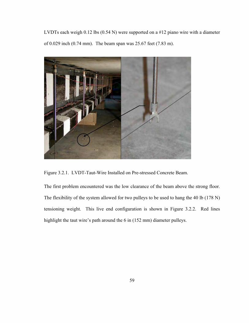
LVDTs each weigh 0.12 lbs (0.54 N) were supported on a #12 piano wire with a diameter
of 0.029 inch (0.74 mm). The beam span was 25.67 feet (7.83 m).
Figure 3.2.1. LVDT-Taut-Wire Installed on Pre-stressed Concrete Beam.
The first problem encountered was the low clearance of the beam above the strong floor.
The flexibility of the system allowed for two pulleys to be used to hang the 40 lb (178 N)
tensioning weight. This live end configuration is shown in Figure 3.2.2. Red lines
highlight the taut wire’s path around the 6 in (152 mm) diameter pulleys.
59

Figure 3.2.2. Live End Pulleys Installed on Prestressed Concrete Beam.
Plots of the deflected shape are shown for different loading levels in Figure 3.2.3. Figure
3.2.4 shows a comparison of three displacement measurements at mid-span. Two were
obtained by LVDTs mounted to the floor and within the test frame. The other is the mid-
span measurement of the LVDT-taut-wire setup.
60

Taut-Wire Displacement vs Load
-4.0
-3.5
-3.0
-2.5
-2.0
-1.5
-1.0
-0.5
0.0
Dis
plac
emen
t (in
.)
0 Kips
10 Kips
20 Kips
30 Kips
40 Kips
50 Kips
60 Kips
70 Kips
80 Kips
90 Kips
100 Kips
110 Kips
120 Kips
130 Kips
133 Kips
Figure 3.2.3. T-Beam Deflected Shapes.
Load vs Deflection at Midspan
0
20
40
60
80
100
120
140
-4.0-3.5-3.0-2.5-2.0-1.5-1.0-0.50.0
Displacement (inches)
Load
(kip
s)
LVDT-Taut Wire midspanActuator LVDT midspanFixed LVDT midspan
Figure 3.2.4. T-Beam capacity Curve. 61

62
While there is a difference in the deflections in Figure 3.2.4, this is likely attributed to
systematic inequalities—each LVDT is measuring at a different location within the cross-
section of the beam. In particular, the taut wire supported LVDT is actually measuring
the slab deflection away from the web of the beam. Upward curling of the unsupported
flange or rotation of the beam in the frame could be causing the observed displacement
discrepancies. It is the author’s opinion that it is not due to any under performance of
either system to capture the displacements. When comparing the cracking behavior
displacement jumps at the higher loads, the relative displacements at those levels are
essentially equivalent.
3.2.2 North Halawa Valley Viaduct (H3 Freeway) Field Installation
This test application was the first attempt at using the LVDT-Taut-Wire system on a long
span. Chapter 8 describes the overall instrumentation used on the viaduct as well as the
goals of the instrumentation program as it relates to SHM. During the instrumentation
program, four manually observed taut-wire baseline systems were installed on four
different spans along the viaduct—which was of prestressed segmental box construction.
During the course of the program, the need for an automated system became apparent.
After testing the LVDT-Taut-Wire system in the laboratory environment, a single span of
the NHVV was instrumented. There were several attempts to get the system to work. At
the end of the system development, the investigators concluded that the system was
viable for measuring deflections of long span beams with reasonable success.

63
The manual taut-wire system installed used #8 gauge piano wire—diameter 0.020” (0.51
mm). The beam span is 360 ft (110 m) from center to center of support. The taut-wire
baseline span was approximately 340 ft (104 m). The live end pulley used was 3 inches
(76 mm) in diameter supporting an 80 lbs (356 N) tensioning weight. This system was
installed within 6 inches (152 mm) of the bottom of the top slab.
Incorporating the LVDTs into the system required several changes. The baseline was
lowered to 24 inches below the top slab to accommodate the length of the LVDT coil
housing and cores. Pulleys installed were 6 inches (152 mm) in diameter to ensure less
influence from friction and wire flexing. After securing the coil housing to the slab
soffit, the cores were attached by eye loops onto the LVDT. The cores of the LVDTs
each weigh 0.12 lbs (0.54 N). During the installation, as the LVDT cores were placed
onto the taut wire significant deflection on the order of several inches occurred at each
location. Data was collected from the system for a short time period—the investigators
were in the box girder when truck traffic crossed the bridge. Typical traffic loading
should cause deflections of up to a quarter inch (6 mm). The data showed that the
displacements observed were much smaller than expected. Also, there were residual
displacements measured. It was clear that the friction between the core and the coil
housing was greater than the restoring force of the very flexible taut wire baseline. This
was visually confirmed by plucking the baseline at the location of one of the LVDTs; the
core oscillated a few times then ceased moving before it could damp out as one would
expect.
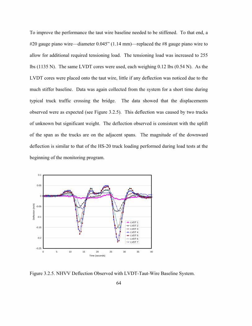
To improve the performance the taut wire baseline needed to be stiffened. To that end, a
#20 gauge piano wire—diameter 0.045” (1.14 mm)—replaced the #8 gauge piano wire to
allow for additional required tensioning load. The tensioning load was increased to 255
lbs (1135 N). The same LVDT cores were used, each weighing 0.12 lbs (0.54 N). As the
LVDT cores were placed onto the taut wire, little if any deflection was noticed due to the
much stiffer baseline. Data was again collected from the system for a short time during
typical truck traffic crossing the bridge. The data showed that the displacements
observed were as expected (see Figure 3.2.5). This deflection was caused by two trucks
of unknown but significant weight. The deflection observed is consistent with the uplift
of the span as the trucks are on the adjacent spans. The magnitude of the downward
deflection is similar to that of the HS-20 truck loading performed during load tests at the
beginning of the monitoring program.
-0.25
-0.2
-0.15
-0.1
-0.05
0
0.05
0.1
0 5 10 15 20 25 30 35 40
Time (seconds)
Def
lect
ion
(inch
)
LVDT 1LVDT 2LVDT 3LVDT 4LVDT 5LVDT 6LVDT 7
Figure 3.2.5. NHVV Deflection Observed with LVDT-Taut-Wire Baseline System.
64
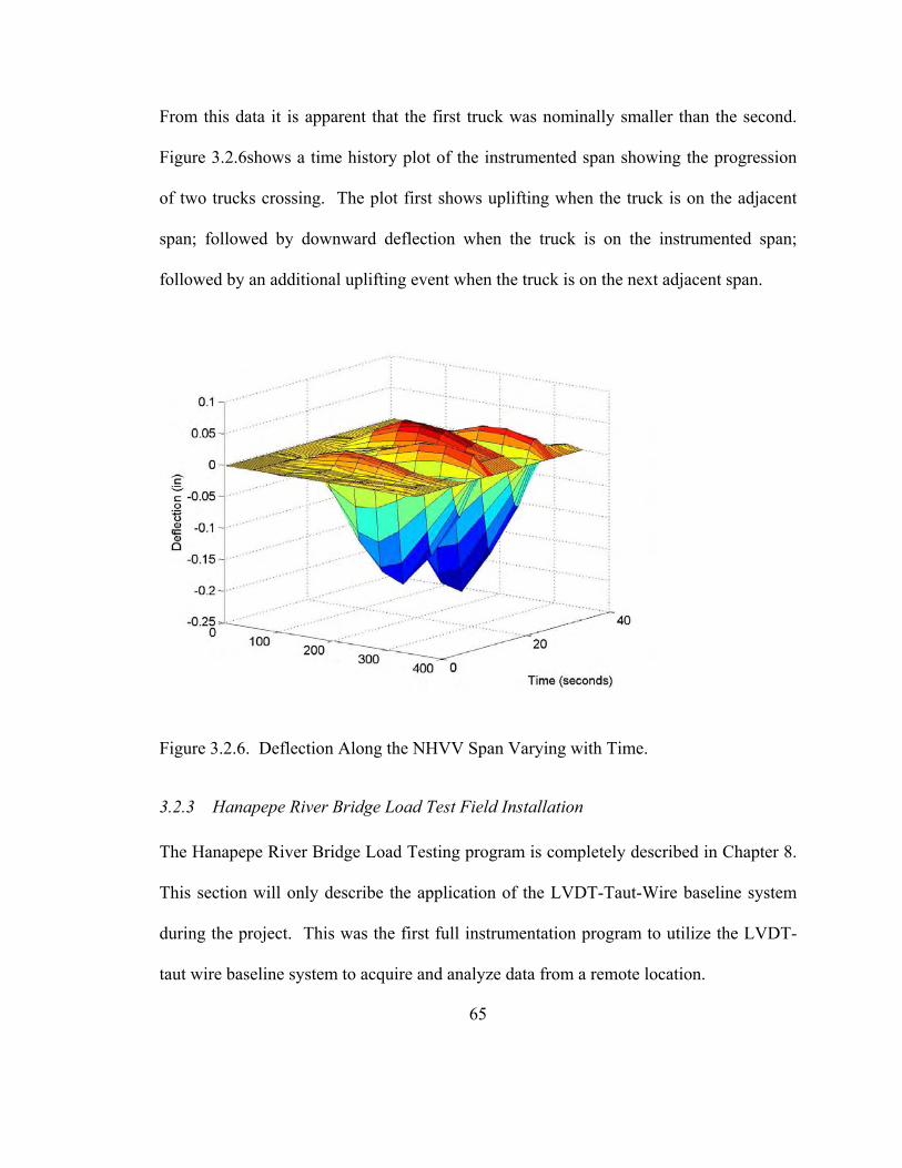
From this data it is apparent that the first truck was nominally smaller than the second.
Figure 3.2.6shows a time history plot of the instrumented span showing the progression
of two trucks crossing. The plot first shows uplifting when the truck is on the adjacent
span; followed by downward deflection when the truck is on the instrumented span;
followed by an additional uplifting event when the truck is on the next adjacent span.
Figure 3.2.6. Deflection Along the NHVV Span Varying with Time.
3.2.3 Hanapepe River Bridge Load Test Field Installation
The Hanapepe River Bridge Load Testing program is completely described in Chapter 8.
This section will only describe the application of the LVDT-Taut-Wire baseline system
during the project. This was the first full instrumentation program to utilize the LVDT-
taut wire baseline system to acquire and analyze data from a remote location.
65

Figure 3.2.7 shows the placement in elevation of one of the two taut wire-LVDT
baselines implemented during the load testing of the Hanapepe River Bridge. The two
baselines were installed on adjacent spans to capture the deflected shape of a single
girder. Figure 3.2.8 shows a section of the bridge with the placement of the baseline
adjacent to girder G-3. The baselines were placed next to the beams to minimize wind
induced vibration of the system. That placement also allowed for the continuous use of
the Hanapepe River for recreational users. Figure 3.2.9 shows the installed dead and live
end supports of the taut wire baseline used.
Figure 3.2.7. Abutment Span Elevation of Girder G-3: LVDT-Taut-Wire Baseline
System.
66

Figure 3.2.8. Bridge Cross-Section: LVDT-Taut-Wire Baseline Adjacent to Girder G-3.
Figure 3.2.9. Taut-Wire Baseline Dead (Left) and Live (Right) End Supports.
67

68
3.3 System Sizing Considerations
When designing a LVDT-taut-wire baseline system, there are several things to consider.
The purpose for using the system is to measure displacement. LVDTs have a wide range
of total measurable displacement capabilities and corresponding displacement
resolutions. In most cases, the LVDT resolution will not be achieved when mounted onto
a taut-wire baseline. The cause is from two general sources: environmentally-induced
movement of the baseline; systematic error induced by the interaction between all the
parts of the system. One of the environmental error sources includes excitation of the
baseline by the wind. The primary source of systematic error is loading of the taut wire
baseline. When the baseline is subjected to a transverse load, the profile will change.
The change is induced to satisfy static equilibrium. The designed strategy discussed here
is a rule of thumb process determined from the experience of the three implementations
tried in section 3.2. The suggested quantitative design process requires incorporating the
span of the taut wire baseline, an estimate of the maximum static friction force applied to
the baseline by the free core LVDT, and a conservative desired resolution of
measurement. These three factors will determine the minimum tensioning load to
achieve the desired resolution. After finding the required tensioning load, the wire size
can be determined.
3.3.1 Implemented System Comparisons
The quantitative design process was determined by observing successful and
unsuccessful implementations of several LVDT-taut wire baseline systems. A total of 27

LVDTs were installed on five different taut wire baselines. When the following analysis
started, it was understood that the largest source of deflection error would occur at the
mid-span of the baseline system—where the weight of the core will cause the largest
displacement. Table 3.1 shows the results of the determination of the displacement of the
baseline system due to the weight of an LVDT core. The displacement was calculated by
satisfying static equilibrium. The calculations were performed for an LVDT at mid-span
of the five different baseline cases (column 1) used during the course of this research.
Columns 2 through 5 are the self weight of the LVDT core, Wcore; length of the
baseline, L; position of the LVDT on the baseline, x; and Tensioning load in the taut
wire, T, respectively. These were used to calculate the deflection, d, under the LVDT
due to the core’s weight—listed in column 6. Column 7 and 8 are a ratio of the span of
the baseline to the deflection and a ratio of the tensile load to the deflection. These ratios
were used to identify which parameter best correlates with the good or bad performance
of the evaluated systems. Columns 9 describes if the system performed adequately and
column 10 states the assumed cause of poor performance.
Table 3.1. Summary of LVDT Core-Induced Baseline Displacement.
69
The system that performed the poorest was the second case at the North Halawa Valley
Viaduct (NHVV-80) with an 80 pound tensioning load. In Table 3.1, the T/d ratio
(column 8) corresponds best with the performance of the system (column 9). During the
initial installation and data acquisition, it was noticed that the LVDT core caused a fairly
large displacement of the baseline system. While the investigators were still in the field,
it was observed that an LVDT was only recording about a 0.05 inch displacement at mid-
span when a large truck was traversing the span. An approximate visual observation of a
parallel manually read taut-wire baseline indicated that the true displacement was closer
to 0.25 inch. This is consistent with the deflection caused by a single AASHTO HS-20
truck load. Upon closer inspection, it was observed that the core was restricted by
friction (see section 3.2.2). Knowing the geometry of the system, the tension load, and
the approximate error caused by friction, an estimate of the friction force, Pf, was
determined. The typical deflected shape including the self weight is controlled by statics.
The deflected shape is shown in Figure 3.3.1 below. The moment caused by the core at
mid-span, Mc = Pf L/4, is determined; the displacement of the baseline at mid-span is
calculated by equation (3.3.1). The deflection at any point along the length of the
baseline is equal to the load-induced moment at that point divided by the tensioning
force:
TxMxd /)()( = . (3.3.1)
70

Figure 3.3.1. Geometry of Deflection and Loads Applied to the Taut-Wire Catenary.
Substituting Mc for M(x) and solving for the friction force, Pf:
LTd
fP 4= . (3.3.2)
Applying a displacement error of 0.20 inch to the NHVV-80 LVDT-Taut-Wire system,
the maximum friction force estimate is:
lb015.0)ft(12in/ft345)in20.0)(lb80(4
==fP .
Using this friction force, Table 3.2 was generated to estimate the baseline deflection
caused by the LVDT core at each location installed for all five baselines tested. The lab
beam test LVDTs were used as described in section 3.2.1; the NHVV-80 and NHVV-240
LVDTs were used as described in section 3.2.2; the Hanapepe-1 and Hanapepe-2 LVDTs
were used as described in section 3.2.3 and chapter 7.
71
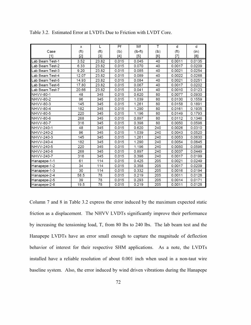
Table 3.2. Estimated Error at LVDTs Due to Friction with LVDT Core.
Column 7 and 8 in Table 3.2 express the error induced by the maximum expected static
friction as a displacement. The NHVV LVDTs significantly improve their performance
by increasing the tensioning load, T, from 80 lbs to 240 lbs. The lab beam test and the
Hanapepe LVDTs have an error small enough to capture the magnitude of deflection
behavior of interest for their respective SHM applications. As a note, the LVDTs
installed have a reliable resolution of about 0.001 inch when used in a non-taut wire
baseline system. Also, the error induced by wind driven vibrations during the Hanapepe
72

73
testing kept the LVDT cores in motion and likely was the greatest source of error for any
single data point.
3.3.2 Suggested Design Process
SHM practitioners should be aware that this outlined design process considers only one
of many possible sources of error that could be induced in a particular system. This
process quantifies the experience of the investigators who use this only as a rule of thumb
calculation. Further research into identifying and quantifying all the error sources and
interaction of multiple errors is planned.
The overall process involves the following steps: determine the maximum expected static
friction force, or force applied to the taut wire baseline; determine the moment induced
by friction of a single LVDT at mid-span of the taut-wire baseline; calculate the
minimum required tensioning load that will provide a conservative resolution of
displacement; select the taut wire size, pulley, and placement.
There is no one way to determine the maximum expected friction force of the system. It
can be done by performing a theoretical calculation. It could be done by systematically
following the process used in section 3.3.1—place the LVDTs on the taut-wire baseline
and measure the deflection error with an accurate parallel system. The friction could also
be determined with a classical friction measurement laboratory test setup.
The moment of the loads applied to the baseline system can easily be determined by
statics. Use the estimated friction force to determine the maximum moment at the

location of the LVDT. The worst case for any system will occur when an LVDT is
located at the mid-span of the baseline. The maximum moment of a point load at mid-
span on a catenary is: M = PL/4. Pf is the friction force; L is the length of the baseline.
Substituting PfL/4 into equation (3.3.1) and solving for the tensile load, T:
resdLfP
T4
= . (3.3.3)
The displacement, dres, should be a conservative resolution desired of the LVDT-Taut-
Wire baseline system. A conservative resolution is some displacement smaller than the
minimum needed resolution. It should be noted that the system is not truly loaded by just
one friction force. Each LVDT applies a friction force. The friction force will not be a
maximum at every reading. Not all the LVDTs will have the same friction force acting
on the baseline at the same time. The tensile load calculated by equation (3.3.3) should
be considered a minimum load. If a larger load is practical, it will provide a better
resolution.
Several considerations should be considered while choosing a wire size. Obviously, the
tensile strength of the wire is important and easily considered with mechanics of
materials and equation (3.3.4).
wireATa /=σ . (3.3.4)
where,
74

σa is the axial stress caused by the tension in the wire,
T is the tension in the wire, and
Awire is the cross-sectional area of the wire.
While considering the wire size, the pulley should be appropriately sized such that its
radius does not yield the wire as it is bent by the tensioning load. The stress at the
extreme fiber induced by bending the wire around the pulley can be calculated by
equation (3.3.5). The sum of equations (3.3.4) and (3.3.5) should be less than the yield
stress of the wire material.
RErb /=σ . (3.3.5)
where,
σb is the longitudinal stress at the extreme fiber of the wire caused by bending,
E is the wire materials elastic modulus,
r is the radius of the wire, and
R is the radius of the pulley plus the radius of the wire.
The baseline profile should be checked: the profile calculation should include both the
maximum sag due to wire self-weight and the additional displacement due to weight of
the LVDT cores. Although elastic deformation obviously occurs, this is taken up by the
75

76
pulley during the addition of the tensioning weight. A sufficiently accurate baseline
profile can be calculated by satisfying statics along the length of the beam.
Other consideration such as pulley friction, dynamic interaction with the attached
structure, and other concerns are not yet considered for this system. A similar system
called a weighted-stretched-wire system (WSWS) [Stanton et al. 2003] was modeled
including the above considerations; this was noted in the literature review section of this
chapter (section 3.1).

77
CHAPTER 4. WHEATSTONE BRIDGE DEVICE DESIGN
4.1 Background
During the course of a structural health monitoring program it is common for
observations of one phenomenon to cause the investigators to focus on a new
phenomenon. In some cases, the increase in scope might not be matched with an increase
in budget. New devices may be needed. Most of the time, buying a device is the best
option because the time involved in the development is more costly than the device—
sometimes this is just not an option. When this happens, there are often solutions that
allow the researcher to “go back to the basics” of instrumentation design and
measurement. This can mean using the cheaper transducers such as strain gauges to
measure other phenomenon such as pressure, or load, or crack opening movement, or
torsion, et cetera. This chapter describes two devices that the author designed and built to
allow more data to be collected for a project with a limited budget. Both devices use four
strain gauges in a Wheatstone bridge to measure deflection. While the principles used to
build the devices are not new, it is useful information to help other researchers and
engineers to improvise solutions when needed. The first device described is a crack
gauge that is used to monitor the crack mouth opening displacement on concrete
structures. The second device described measures deflection at a very fine resolution—
two were used to measure the relative rotation of a pinned connection between the top of
a pier and a bridge superstructure.

78
4.2 Crack Gauge Device
Concrete structures crack. Cracking in a reinforced concrete structure forces the
reinforcing steel to maintain the load carrying capacity of the structure in tension. Due to
environmental concerns, specifically reinforcing corrosion, the ACI Committee 224
report provides a guide for the maximum tolerable flexural crack width in various
environmental conditions [Nawy 2000]. Engineers currently use visual crack
comparators—clear plastic cards with multiple lines of various widths—to determine the
crack width in existing structures. They use visual crack “monitors” to observe the crack
opening overtime via the initial alignment of crosshairs. These devices cannot provide
information on whether a crack is active while under load, or if the crack is merely a
result of initial restrained shrinkage—of no analytical capacity reducing consequence. A
crack mouth opening displacement (CMOD) observable during a load test provides a
quantitative indicator of a detrimental condition.
There exist commercially available electronic crack meters that can easily be integrated
into a data acquisition system. In the laboratory, they can be very useful in determining
the material properties of fiber reinforced composite materials, for testing of cracked
concrete structural elements, for observing crack opening behavior related to fracture
mechanics, et cetera. Each of these devices must be installed after the initiation of the
crack and is not generally robust enough or cost effective for longer term field
installation.

79
During the course of this research, the need for monitoring the movement of multiple
cracks on an existing bridge became an issue. During the Hanapepe River Bridge load
test program a new crack gauge device was designed and evaluated as an alternative to
the commercially available devices. The investigators chose to build them, instead of
buying them, to reduce the cost of the instrumentation installation. The cost of strain
gauges is very small compared to that of the commercially available crack gauges. Harris
and Piersol [2002] describes various ways to use strain gauges to measure displacement.
In particular, they describe using a C-shaped spring to monitor the displacement of its
two legs [Harris & Piersol 2002, pg 17.8]. The design and construction of one such
device is shown here. By building these devices ten times as many crack locations can be
monitored for the same cost. Also, they can be designed per application to achieve a
better resolution on the same data acquisition system.
4.2.1 Design Basis
The crack gauges described in this section were built with the intent to provide an
economical, reliable, and robust device to withstand a field installation. The concept is
based on using bending strain to amplify the relative movement between two locations.
Using a bending based gauge provides a higher resolution than an axial based gauge.
Four strain gauges are used to monitor the flexural strain within the device. The crack
gauge was designed and built based on a full Wheatstone bridge configuration of
electrical resistance strain gauges (see Chapter 2.3.1.1.2).

80
4.2.2 Physical Specifications
The devices were built using Vishay Micro-Measurements CEA-06-125UN-350 foil
strain gauges. Two gauges were mounted side by side on one face of the device such that
when the distance between the legs of the gauge increases they are in tension. At the
same time, the other two gauges are in compression and in a similar configuration on the
opposite face. Again, the gauges are oriented so that they theoretically experience the
same level of flexural straining—opposite signs for opposing faces on the device. The
gauges were connected in a full Wheatstone bridge configuration using 30 gauge wire.
The wiring diagram indicating strain direction (+ε or -ε) of each gauge is shown in Figure
4.2.1. The configuration used maximizes the signal voltage based on a given change in
strain—four times the output signal of a single strain gauge in a quarter Wheatstone
bridge configuration. The full bridge and placement configuration of the gauges
automatically compensates for the thermal output of all the strain gauges—including
coefficient of thermal expansion mismatch. Any thermal effect occurs on all four legs of
the circuit negating any change at the signal voltage (see Chapter 2.3.1.1.2). Axial
straining does not contribute toward the signal voltage either.
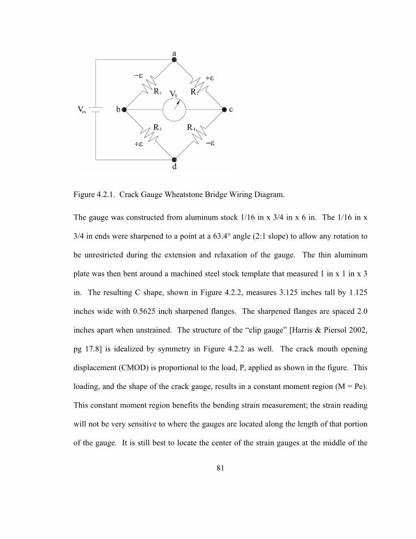
Figure 4.2.1. Crack Gauge Wheatstone Bridge Wiring Diagram.
The gauge was constructed from aluminum stock 1/16 in x 3/4 in x 6 in. The 1/16 in x
3/4 in ends were sharpened to a point at a 63.4° angle (2:1 slope) to allow any rotation to
be unrestricted during the extension and relaxation of the gauge. The thin aluminum
plate was then bent around a machined steel stock template that measured 1 in x 1 in x 3
in. The resulting C shape, shown in Figure 4.2.2, measures 3.125 inches tall by 1.125
inches wide with 0.5625 inch sharpened flanges. The sharpened flanges are spaced 2.0
inches apart when unstrained. The structure of the “clip gauge” [Harris & Piersol 2002,
pg 17.8] is idealized by symmetry in Figure 4.2.2 as well. The crack mouth opening
displacement (CMOD) is proportional to the load, P, applied as shown in the figure. This
loading, and the shape of the crack gauge, results in a constant moment region (M = Pe).
This constant moment region benefits the bending strain measurement; the strain reading
will not be very sensitive to where the gauges are located along the length of that portion
of the gauge. It is still best to locate the center of the strain gauges at the middle of the
81

constant moment region—this helps to reduce the effects of a small amount of
unintentional twisting.
Figure 4.2.2. Crack Gauge Design and Loading Diagram.
The most important considerations to obtain good, consistent, readings are three fold:
align the sensitive axis of the strain gauge with the axis of the aluminum plate; provide an
even loading (at P) to prevent twisting; and provide effective strain relief at the cable
connection such that the cable will not pull on the gauge as loading occurs. Proper strain
gauge alignment will be achieved with good strain gauge installation technique. Figure
4.2.3 shows the strain relief that was provided during an installation at the Hanapepe
River Bridge (see Chapter 7). The strain relief was simply a large washer clamping
against the concrete surface. Notice the slack of the cabling between the crack gauge and
the strain relief is minimal but not tight.
82

Figure 4.2.3. Crack Gauge Installations.
Finally, the crack gauge is attached to the concrete surface by epoxying two 1 in x 1 in x
0.5 in aluminum blocks as seen in Figure 4.2.3. They are accurately spaced by using a
1/8 inch thick gauge spacer while the quick setting epoxy is curing. This spacer performs
two functions. First, it ensures a consistent pretension for each gauge to support its own
weight, as well as, allows for crack closure to be measured. Second, it allows for the tips
of the crack gauge to sit flush and firm within the 90° triangular groove milled into the
two aluminum blocks (see Figure 4.2.3). The 90° grove is used to lock the gauge into a
stable position. It also allows for the rotation of the 63.4° beveled edge during the
83

84
extension and contraction of the crack mouth. Using a sharp edge minimizes any friction
or rotational restraint that would induce a moment into the tips of the crack gauge.
4.2.3 Estimating Crack Mouth Opening Displacement (CMOD) Resolution
The vertical deflection due to bending caused by the load, P, of the idealized system in
Figure 4.2.2 is easily calculated by the moment-area method. The maximum moment can
be expressed as a function of strain within the deflection solution equation. The
maximum moment occurs at the fixed support in the idealized model; in the real crack
gauge structure the strain gauges are attached at this location. The deflection of the
idealized model is equal to one-half the total CMOD observed with the crack gauge. To
estimate the CMOD resolution of the gauge; first, the structural strain response of the
gauge must be understood; then, the resolution of the strain gauge technology must be
used as the strain input for the deflection calculation.
To establish the relationship between deflection and strain, first, the deflection due to an
unknown load, P, should be determined. The load, P, is shown in Figure 4.2.2. Only the
bending strain will be observed by the Wheatstone bridge used in the device. Therefore,
only the vertical deflection resulting from the load P will be considered. It is assumed
this displacement is of a much larger magnitude than any axial straining. The moment
diagrams are shown in Figure 4.2.2. The maximum moment is equal to the load, P,
multiplied by the eccentricity, e, of that load to the idealized fixed support. The area
under the moment diagrams—normalized by the flexural rigidity, EI—is calculated
below:

⎟⎠⎞
⎜⎝⎛=
21e
EIPeψ (4.2.1)
⎟⎠⎞
⎜⎝⎛=
22h
EIPeψ (4.2.2)
In equation (4.2.1) and equation (4.2.2): ψ1 is the change in the angle of rotation across
the horizontal flange of the gauge; ψ2 is the change in the angle of rotation across the
vertical leg at the fixed support of the idealized structure; e is shown in Figure 4.2.2 as
the eccentricity of the load P to the fixed support; h is the distance, shown in Figure 4.2.2,
between the centroids of the two horizontal flanges of the crack gauge.
The vertical deflection of the idealized structure, equal to one-half the CMOD observed
by the crack gauge, is given as:
( )eeCMOD23
212
ψψ +⎟⎠⎞
⎜⎝⎛= . (4.2.3)
Substituting equations (4.2.1) and (4.2.2) into equation (4.2.3) gives:
( )eEI
PeheEI
PeCMOD23
22
2
2+⎟
⎠⎞
⎜⎝⎛= ,
Simplifies to:
⎟⎠⎞
⎜⎝⎛ +=
23
2
2he
EIPeCMOD , or,
85

⎟⎠⎞
⎜⎝⎛ += he
EIPeCMOD
322
. (4.2.4)
From mechanics of materials, the flexural formula, I
Myx −=σ , can be combined with
Hooke’s law, xEx εσ = , to relate the bending moment to the strain. Substituting the
magnitude of the moment at the location of the strain gauges, Pe; and one-half the
aluminum plate thickness, t/2, for -y; the following results:
xtEIPe ε2
= . (4.2.5)
Finally, substituting equation (4.2.5) into equation (4.2.4), the crack mouth opening
displacement as a function of strain due to bending at the location of the strain gauges is:
xtheeCMOD ε2
32
⎟⎠⎞
⎜⎝⎛ += , or,
xtheeCMOD ε⎟
⎟
⎠
⎞
⎜⎜
⎝
⎛+=
23
24 . (4.2.6)
From equation (4.2.6), it can be seen that the crack gauge sensitivity—in parenthesis—is
solely dependant on the geometry of the gauge. If a greater sensitivity is required,
increasing the eccentricity, e, will produce the greatest effect: increasing the gauge
height, h, or decreasing the gauge plate thickness, t, will also increase the crack gauge
sensitivity. Finally, for the crack gauge shown in Figure 4.2.2, the crack gauge
86

87
sensitivity, can be calculated using e = 1.09375”, h = 3.0625”, and t = 0.0625”. The
resulting gauge sensitivity is 109 inches. A reasonable strain resolution of the full
Wheatstone bridge is 2 microstrain; the smallest observable CMOD for that resolution of
strain is 109 in (0.000002) = 0.000218 inches. During the calibration of the gauges built
during this research program, the CMOD measurement resolution obtained was 0.00022
inches.
4.3 Rotation Monitoring by Deflection Device
In the structural health monitoring field, it is advantageous to run two, or more, systems
in a side by side comparison. For example, it is common to measure deflections by an
optical survey at the same time as recording the deflections with a SHM data acquisition
system. One data set can validate or backup the other. A side by side comparison can
also be performed between two transducer based systems—an established system can
help to validate a newer technique. The rotation monitoring device described in this
section was used to augment, or fill in the gaps, between two LVDT-Taut-Wire baseline
systems that monitored the deflected shape of the Hanapepe River Bridge. The
instrumentation is fully described in chapter 7.
4.3.1 Design Basis
The displacement gauges described in this section were built with the intent to provide a
cheap, reliable, and robust device to withstand a field installation. The concept is based
on using bending strain to amplify the relative movement between two locations. Using a
bending based gauge provides a higher resolution than an axial based gauge. Four strain

88
gauges are used to monitor the flexural strain within the device. The displacement gauge
was designed and built based on a full Wheatstone bridge configuration of electrical
resistance strain gauges (see Chapter 2.3.1.1.2).
4.3.2 Physical Specifications
The strain gauges used and their configuration are the same as those used for the crack
gauges described in section 4.2. The configuration provides an accurate measurement of
displacement based on strain magnification induced by bending. The wiring provides
temperature compensation.
The gauge was constructed from aluminum stock 1/16 in x 3/4 in x 12 in. A 3/8 in
diameter hole is drilled into each end of the plate. The center of the holes are located 3/4
of an inch from the end of the plate. The thin aluminum plate was then bent around a
machined steel stock template that measured 1 in x 1 in x 3 in to form a C shape. The
two ends are then bent back parallel to the 3 inch portion of the bent plate. The resulting
shape, shown in Figure 4.3.1, measures 10 inches tall by 1.0625 inches wide 3.5 inch
long flanges.
The gauge is designed to measure the relative movement between the 3.5 in flanges—
measuring the change in distance between the two 3/8 in diameter holes at each end. To
do this effectively, care must be taken to ensure the deflected shape of the device is
symmetrical and consistent. The 1.5” long steel clamps on each side and each end of the
device are used to establish consistent boundary conditions for each installation. The

holes are used to allow a single 3/8 diameter bolt to provide a clamping force to the 1/2
inch thick steel plates.
Similar to the structure of the crack gauge, in section 4.2, the displacement is
proportional to the load applied to extend or contract the device. The loading and the
shape of the gauge creates a constant moment region at the location of the strain gauges.
This constant moment region benefits the bending strain measurement; the strain reading
will not be very sensitive to where the gauges are located along the length of that portion
of the gauge. It is still best to locate the center of the strain gauges at the middle of the
constant moment region—this helps to reduce the effects of a small amount of
unintentional twisting.
Figure 4.3.1. Deflection Gauge For Monitoring Pin Connection Rotation.
89
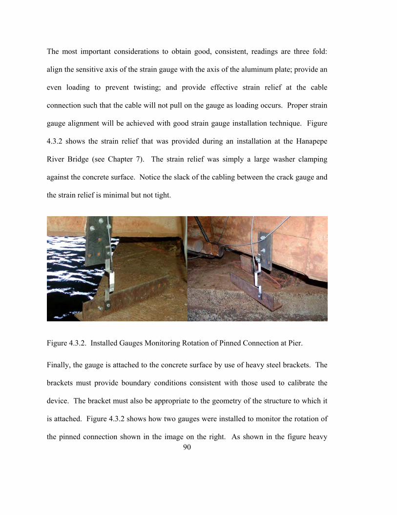
The most important considerations to obtain good, consistent, readings are three fold:
align the sensitive axis of the strain gauge with the axis of the aluminum plate; provide an
even loading to prevent twisting; and provide effective strain relief at the cable
connection such that the cable will not pull on the gauge as loading occurs. Proper strain
gauge alignment will be achieved with good strain gauge installation technique. Figure
4.3.2 shows the strain relief that was provided during an installation at the Hanapepe
River Bridge (see Chapter 7). The strain relief was simply a large washer clamping
against the concrete surface. Notice the slack of the cabling between the crack gauge and
the strain relief is minimal but not tight.
Figure 4.3.2. Installed Gauges Monitoring Rotation of Pinned Connection at Pier.
Finally, the gauge is attached to the concrete surface by use of heavy steel brackets. The
brackets must provide boundary conditions consistent with those used to calibrate the
device. The bracket must also be appropriate to the geometry of the structure to which it
is attached. Figure 4.3.2 shows how two gauges were installed to monitor the rotation of
the pinned connection shown in the image on the right. As shown in the figure heavy 90

91
steel angles and steel plates were used. These attachment brackets need to be stiff
enough that the load induced in the gauge by its deformation does not significantly
deform the brackets as well—that measurement will be lost.
4.3.3 Estimating Displacement Resolution
The structural system of the installed gauge is indeterminate to the 3rd degree when
idealized as a two dimensional bent beam. To estimate the displacement resolution, the
relationship between the axial displacement and bending strain at the strain gauge
locations can be analyzed using mechanics of materials principles. The strain
measurement resolution can then be applied to the equation and the displacement
resolution is determined. This process was demonstrated in section 4.2.3 for the crack
gauge device. During the course of development, it was decided that since the two
devices were geometrically quite similar, with a similar mode of loading, a detailed
calculation of the estimated resolution was not necessary. In the end, the resolution of
the device was similar to that of the crack gauge.

92

93
CHAPTER 5. STRAIN GAUGE BASED DEFLECTED SHAPE CALCULATION
Directly observing the relative movement between a structure and a stationary object
during loading seems trivial. However, this cannot always be done easily. Chapter 3
addresses some, but not all, of the difficulties by using a catenary device to establish a
baseline from which to directly measure displacement. In some cases an indirect
measurement is more practical. In structural health monitoring, most transducers
indirectly monitor one phenomenon by observing another. The device’s physical,
electrical, or optical properties are designed such that an easily observable quantity is
amplified with a change of the phenomenon of interest. With this in mind, it should be
possible to use our experience and observations of material behavior to indirectly
measure the displacement of structures. Specifically, we can utilize our knowledge of
constitutive, kinematic and equilibrium relationships. This chapter discusses one method
to calculate the displacement of a beam from discrete observations of longitudinal strain.
5.1 Literature Review
Vurpillot et al. propose a mathematical model to determine the vertical displacements of
beams from internal horizontal deformations—strains [Vurpillot et al 1998]. They
verified their model both in the laboratory, on a timber beam, and in the field, on the
Lutrive Highway Bridge in Switzerland [Vurpillot et al 1998]. They applied a static
uniformly distributed load onto one span of a two span timber beam. The results agreed
well with traditional displacement measurements in the laboratory. They monitored the
Lutrive Highway Bridge, in Switzerland, to verify diurnal temperature deflections of a

94
single cantilever span. The diurnal temperature induced deflections—calculated by their
method—agreed well with an installed hydrostatic deflection monitoring system in the
bridge. The rotation at the end of the cantilever was measured and applied as a boundary
condition to their mathematical model. The temperature loading in this case is very
similar to a uniformly distributed load. The Vurpillot et al. model will work well for
these types of loading conditions. Indeed, by design, their mathematical model is based
on a discretization of the beam into sections; each of which has a constant inertia and a
uniformly distributed load. The application of a concentrated force or a bending moment
must occur at the nodes between the beam sections [Vurpillot et al. 1998]. The
mathematical model assumes a deflected shape that is C1 continuous; fourth order
polynomial—the Bernoulli solution to a uniformly loaded beam [Vurpillot et al. 1998].
The curvature function, for this situation, is a second degree polynomial fit to the strain
based curvature measurements. To determine the curvature function for each section,
they suggest three curvature measurements—preferably at locations with high values of
curvature. They mention that for a triangular distributed load only one additional
curvature measurement is needed. They state that the precision of displacement
measurements can be calculated with a sensitivity study—they conclude with 10
microstrain precision for the strain gauges, a deflection measurement can be obtained
with less than 8% error [Vurpillot et al. 1998, pg 524-526]. Without other
instrumentation systems, the rigid body displacements cannot be obtained—this method
is for measuring internal relative displacements.
95
Cho et al. [2000] also utilize a methodology similar to Vurpilot et al. They apply it to a
simply supported beam with midpoint loading. They obtain strain readings from both
electrical resistance and fiber optic strain gauges to compare their performance. They
convert strain readings to curvature based on the section properties of the beam. They
assume a linear curvature function for each half of the beam based on the known loading
condition. They obtain a best fit of the curvature data with linear regression. They cycle
the load up to 86% of yielding of the steel beam. The results match well between the dial
gauges, electrical resistance strain gauges, fiber optic strain gauges, and the analytical
predictions. They observe a maximum relative error of 8% at one location (of seven)
during one of the smallest levels of loading. Generally, they observe the largest relative
error at the smallest load levels. They attribute this to “unstable settlement of supports”
[Cho et al. 2000, pg 345]. They conclude that this method can be used for measuring
bridge deflections [Cho et al. 2000, pg 346].
Fung and Robertson [2003] applied this method to several beams in a laboratory. They
tested it on a simply supported tube steel beam subjected to four-point loading; a small
scale three-span continuous beam subjected to point loads, support movements, and free
vibration after plucking between beam sections. They also tested the method for several
levels of load on a concrete beam before and after cracking occurred. Each of these
beams was tested using electrical resistance strain gauges. The dynamic measurements
were able to identify the general mode shape and resonant frequency of deflection, but
were not able to identify the magnitude—this was attributed to the type of electric

96
resistance strain gauges used, not the calculation methodology. For all beams they fitted
a second degree polynomial to the curvature data to obtain the curvature function.
Aki and Robertson [2005] applied this system to a small scale three-span continuous tube
steel beam. Fabry-Perot fiber optic strain gauges were evaluated in a side-by-side
comparison with electrical resistance strain gauges on the small scale beam. The
magnitude of the dynamic displacement observed by the fiber optic strain gauges was
similar to the magnitude observed by LVDTs. However, the two interior supports which
were not defined by applied boundary conditions of the mathematical model showed
displacements when there were none. Some of the deflected shapes with large
displacements at these supports were not consistent with the expected mode shape of
vibration. The deflections were “normalized” by shifting the curves such that
normalization forced the displacement at those supports to be zero. The resulting
deflected shapes matched very well with the displacements observed by LVDTs. Using
the small scale steel beam, they also attempted to use the method to observe torsional
displacements—placing four strain gauges at each cross-section. They noted torsional
displacements that were not consistent with the applied loading. For all beams they fit a
second degree polynomial to the curvature data to obtain the curvature function.
5.2 General Methodology
As described in section 5.1, Vurpillot et al. [1998] published the methodology for
converting strain measurements to a deflected shape of a beam. Essentially, strain is
converted to curvature; either based on section properties, or from multiple strain gauges

through the depth of the beam. The method ultimately describes a process that estimates
the curvature function then uses that generated function to calculate the beam
displacement function. To simplify, the methodology will be called the C2D method
from here on. In this chapter, only the C1 continuous fourth-order polynomial
assumption for deflected shape will be considered.
5.3 Curvature to Displacement (C2D) Derivation
From calculus, we know that the curvature of a plane curve is the change in slope per unit
of arc length [Salas 1995, pg 888]. In terms of the standard Cartesian coordinate system,
curvature, κ, is:
3/2]2)'(1[
''
y
y
+=κ . (5.2.1)
where;
y is a function of x, y (x);
y’ is the first derivative of y (x) with respect to x;
y” is the second derivative of y (x) with respect to x.
Generally, in structural engineering, only small deflections are considered. This
simplifies the curvature function to the expression:
"y=κ . (5.2.2)
97
Therefore, the first derivative of the displacement function, y’, provides the functions
slope (angle of rotation); and the second derivative is considered the curvature function.
Let the curvature function be a second degree polynomial:
cbxaxx ++= 2)(κ . (5.2.3)
The coefficients a, b, and c are unknowns. To obtain them, three equations are needed—
three curvature observations at three locations (i = 1, 2, 3) along the length of the beam
section. The curvature observations are determined from strain measurements along the
beam. If the gauge length of the strain measurement is very short, we can assume that
strain occurs at the center of the gauge. Using the x ordinate at the center of the gauge in
equation (5.2.3) is probably appropriate in this case. Evaluate equation (5.2.3) at each “i”
location to create and solve a system of three equations for a, b, and c.
If, however, the gauge length of the strain measurement is long (ex., 1 meter) then the
assumption that the average strain occurs at the center of the strain gauge may not be
appropriate. The true location of the indicated strain cannot be determined; arbitrarily
choosing the x ordinate will generate biased error of unknown magnitude and direction.
Instead, the Mean Value Theorem can be used in combination with equation (5.2.3) to
produce a new equation to rationally choose the coefficients a, b, and c. The new
equation becomes the mean curvature equation:
98

lxrx
rx
lxdxcbxax
m−
∫ ++
=
)2(
κ . (5.2.4)
where;
κm is the mean curvature on the interval from xl to xr.
xl is left most (starting) ordinate of the strain gauge (x increasing to the right);
xr is right most (ending) ordinate of the strain gauge (x increasing to the right).
Integrating equation (5.2.4) produces:
)()22
(2
)33
(3
)( rxlxcrxlxbrxlxarxlxm −+−+−=−κ . (5.2.5)
Evaluate equation (5.2.5) at each “i” location to create and solve a system of three
equations for a, b, and c.
The process of determining a, b, and c is repeated for all of the beam sections in the
model. Again, for this derivation of the C2D method, a beam section will have a constant
flexural rigidity and a uniformly distributed load. Point loads, support reactions, and
applied moments should only be applied at ends of a beam section, or intersection of two
beam sections.
99

Integration of the curvature function—equation (5.2.3)—results in the C0 continuous
third degree polynomial angle of rotation equation:
jxjcxjbxja
dxxjx ακθ +++∫ == 22
33
)()( . (5.2.6)
where;
θ(x)j is angle of rotation as a function of location along beam section;
j is the index for the beam section;
αj is the constant of integration, for beam section j, that is defined by the boundary
conditions with the adjacent beam sections to ensure angle of rotation continuity (due to
C1 continuity of the deflection curve).
Completing the double integration of the curvature function—equation (5.2.3)—results in
the C1 continuous fourth degree polynomial beam section deflection equation:
jxjxjcxjb
xjadxxdxjxjxv βακθ ++++=∫∫=∫= 2
23
64
12)())(()( . (5.2.7)
where;
v(x)j is the beam section deflection function;
βj is the constant of integration, for beam section j, that is defined by the boundary
conditions with the adjacent beam sections to ensure displacement continuity.
100

It is up to the user of the C2D method to decide on the appropriate global boundary
conditions. Only two global boundary conditions need to be assigned to proscribe the
rigid body orientation of the beam. Any additional boundary conditions can be checked
by verifying the displaced shape obtained by the process.
The process for assembly of the entire beam deflection function is up to the user;
however, the following two requirements will ensure the C1 continuity along the entire
length of the beam. The first ensures continuity of displacements; the second ensures
continuity of the angle of rotation:
1)0()( += jvjjlv . (5.2.8)
1)0()( += jjjl θθ . (5.2.9)
If the loading condition is not consistent with the description of the defined beam
sections, the C1 continuous fourth degree polynomial—generated by the double
integration of the curvature functions—may not accurately describe the deflected shape
of the beam. The curvature function, generated by the aforementioned process, should be
consistent with the M/EI diagram of the beam. Any difference will result in erroneous
calculated deflections.
5.4 C2D Method Matlab™ Implementation:
The method used by Vurpillot et al [1998] was incorporated into a Matlab™ program
which uses the locations, lengths, and measurements of strain gauges within each beam
101

102
segment; combines them with boundary condition assumptions; and calculates the
deflected shape of the beam. The method assumes that a C1 continuous fourth degree
polynomial accurately represents the deflected shape. The Matlab™ program assumes
zero deflection at the two end supports, the deflections at the two interior supports are not
forced by boundary conditions. Only two boundary conditions are required to obtain the
solution so the interior support displacements are calculated. Using the cantilever
deflection of the beam, the program determines the initial angle of rotation at the left
support. The program takes into account the length of the strain gauge; in other words,
the Mean Value Theorem based “integral” form of the curvature function approximation
is used as shown in equations (5.2.4) and (5.2.5). The program files are in the Appendix,
section A5.4.
5.4.1 RISA-2D Strain Input
The Matlab™ program is used to perform the calculations and generate some of the
figures in this section. The strain data used in this section are the theoretical strains of the
system shown in Figure 5.4.1. The structural system is a three span continuous beam
identical to that tested by others [Fung & Robertson 2003, Aki & Robertson 2005]. The
strain data was generated from the stresses indicated by a beam finite element (FE) model
using the RISA-2D™ software by RISA Technologies, Inc. The idealized FE model is
shown in Figure 5.4.2.
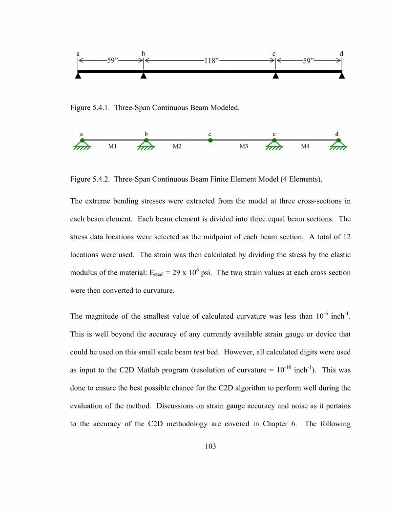
Figure 5.4.1. Three-Span Continuous Beam Modeled.
Figure 5.4.2. Three-Span Continuous Beam Finite Element Model (4 Elements).
The extreme bending stresses were extracted from the model at three cross-sections in
each beam element. Each beam element is divided into three equal beam sections. The
stress data locations were selected as the midpoint of each beam section. A total of 12
locations were used. The strain was then calculated by dividing the stress by the elastic
modulus of the material: Esteel = 29 x 106 psi. The two strain values at each cross section
were then converted to curvature.
The magnitude of the smallest value of calculated curvature was less than 10-6 inch-1.
This is well beyond the accuracy of any currently available strain gauge or device that
could be used on this small scale beam test bed. However, all calculated digits were used
as input to the C2D Matlab program (resolution of curvature = 10-10 inch-1). This was
done to ensure the best possible chance for the C2D algorithm to perform well during the
evaluation of the method. Discussions on strain gauge accuracy and noise as it pertains
to the accuracy of the C2D methodology are covered in Chapter 6. The following
103

104
sections show the performance of the C2D method for several static loading scenarios—
as implemented with the Matlab program in Appendix A5.4.
5.4.2 Evaluated Loading Scenarios
The different scenarios are listed in Table 5.1 below. In the RISA-2D program, each
point load scenario (1 through 3 in Table 5.1) involved a single 5 lb point load. The
results for member forces, member stresses and member deflections were extracted.
They were then scaled by the superposition principle such that the scaled results reflect
the behavior of the same beam with a 1 lb point load. Similarly, for the distributed load
scenarios (4 and 5 in Table 5.1), a 1 lb/in load was applied to the structure. The results
were then divided by a factor of 59 to modify them such that a total load of 1 lb was
acting on the beam—the distributed loads in both scenarios are 59 inches long. This was
done because RISA-2D only reports deflections to the nearest 0.001 inch. The scale
model being tested (Figure 5.4.1 and Figure 5.4.2) and the loads applied (Table 5.1) are
much smaller than the typical members and loads used in this software package—some
of the deflections along the length of the beam are less than 0.001 inches.

Table 5.1. Matlab™ Based C2D Method Evaluation Scenarios.
A summary of the curvatures calculated from the RISA-2D data along the length of the
beam is shown in Table 5.2. The total length of the beam is 236 inches. In this C2D
calculation the gauge length for each strain / curvature reading is accounted for; the
gauge length used was 0.5 inch. This is to compare to strain gauge readings obtained by
on the real structure as discussed in Chapter 6—their gauge lengths are about 0.5 inches.
The actual gauge length varies: the electrical resistance gauges were 1 inch long; the fiber
optic gauges were 0.2 inches long.
Table 5.2. Curvature Observations Used in C2D Program.
105

5.4.3 Matlab Implementation Scenario 1MoCS
This scenario represents a single unit load applied to the middle of the center span of the
structure represented in Figure 5.4.1. The curvature used in the C2D calculation is
reported in Table 5.2 above.
The first step to estimate the curvature function from the discrete curvature measurements
results in Figure 5.4.3. The figure shows three plots. The solid line represents the
theoretical M/EI, or curvature, diagram based on the known loading. The dashed line
with the square data points represents the estimated curvature function. The large solid
circle plot represents the curvature data used as input for the C2D calculation.
Curvature For Unit Point Load at Midspan of Center Span
-0.000008
-0.000006
-0.000004
-0.000002
0.000000
0.000002
0.000004
0.000006
0.000008
0.000010
0.000012
0 59 118 177 236
Distance along Beam (in)
Cur
vatu
re (1
/in)
Discrete CurvatureObservations into MatLab
FE Calculated Curvature(RISA-2D)
Curvature Function(Resolution = 10E-10)
Figure 5.4.3. Scenario 1MoCS: Curvature Estimation.
106

After integrating twice and applying the boundary conditions (zero deflection at nodes
“a” and “d”). Figure 5.4.4 results. The dashed line with the circular data points
represents the deflection calculated by RISA 2-D. The solid line with square data points
represents the deflection calculated by the C2D method.
Deflection For Unit Point Load at Midspan of Center Span
-0.009
-0.008
-0.007
-0.006
-0.005
-0.004
-0.003
-0.002
-0.001
0.000
0.001
0.002
0 59 118 177 236
Distance along Beam (in)
Def
lect
ion
(in)
Deflection Function(Resolution = 10E-10)
RISA 2D Deflection
Figure 5.4.4. Scenario 1MoCS: Deflection Comparison.
Both the curvature and deflection are well represented for this load condition.
5.4.4 Matlab Implementation Scenario 1MoAS
This scenario represents a single unit load applied to the middle of the abutment span of
the structure represented in Figure 5.4.1. The curvature used in the C2D calculation is
reported in Table 5.2 above.
107
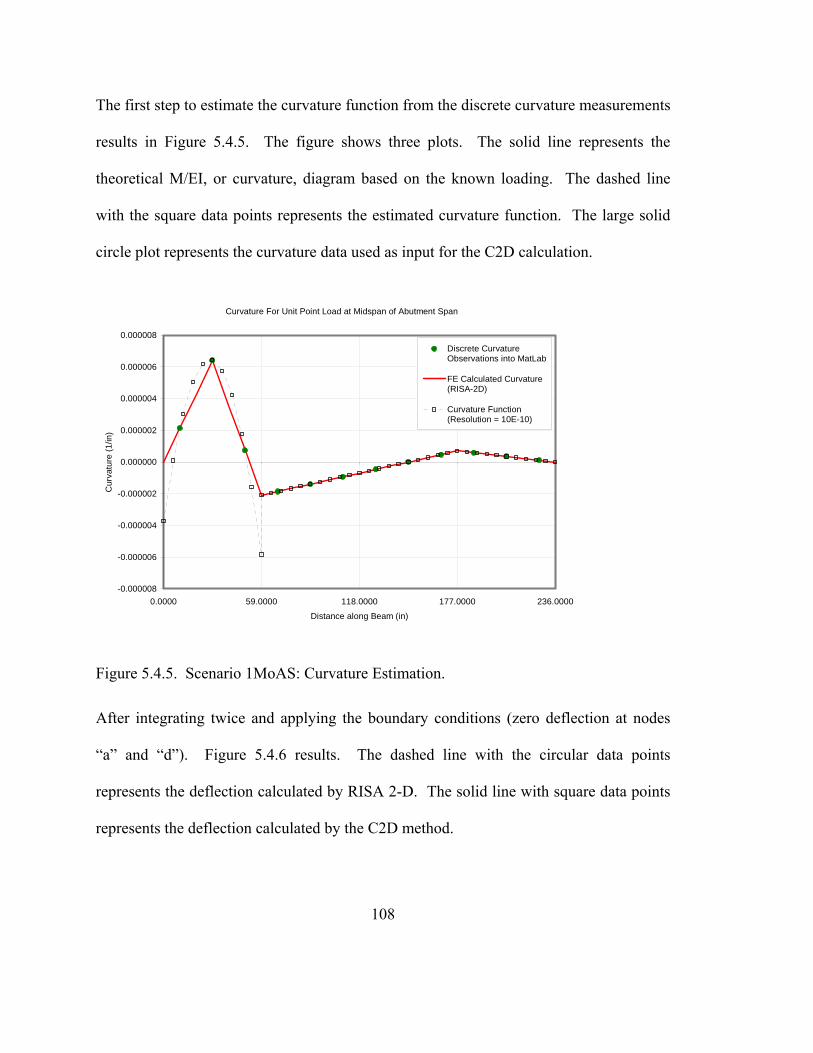
The first step to estimate the curvature function from the discrete curvature measurements
results in Figure 5.4.5. The figure shows three plots. The solid line represents the
theoretical M/EI, or curvature, diagram based on the known loading. The dashed line
with the square data points represents the estimated curvature function. The large solid
circle plot represents the curvature data used as input for the C2D calculation.
Curvature For Unit Point Load at Midspan of Abutment Span
-0.000008
-0.000006
-0.000004
-0.000002
0.000000
0.000002
0.000004
0.000006
0.000008
0.0000 59.0000 118.0000 177.0000 236.0000
Distance along Beam (in)
Cur
vatu
re (1
/in)
Discrete CurvatureObservations into MatLab
FE Calculated Curvature(RISA-2D)
Curvature Function(Resolution = 10E-10)
Figure 5.4.5. Scenario 1MoAS: Curvature Estimation.
After integrating twice and applying the boundary conditions (zero deflection at nodes
“a” and “d”). Figure 5.4.6 results. The dashed line with the circular data points
represents the deflection calculated by RISA 2-D. The solid line with square data points
represents the deflection calculated by the C2D method.
108
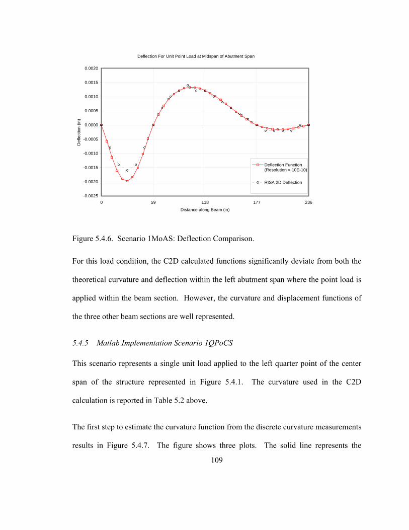
Deflection For Unit Point Load at Midspan of Abutment Span
-0.0025
-0.0020
-0.0015
-0.0010
-0.0005
0.0000
0.0005
0.0010
0.0015
0.0020
0 59 118 177 236
Distance along Beam (in)
Def
lect
ion
(in)
Deflection Function(Resolution = 10E-10)
RISA 2D Deflection
Figure 5.4.6. Scenario 1MoAS: Deflection Comparison.
For this load condition, the C2D calculated functions significantly deviate from both the
theoretical curvature and deflection within the left abutment span where the point load is
applied within the beam section. However, the curvature and displacement functions of
the three other beam sections are well represented.
5.4.5 Matlab Implementation Scenario 1QPoCS
This scenario represents a single unit load applied to the left quarter point of the center
span of the structure represented in Figure 5.4.1. The curvature used in the C2D
calculation is reported in Table 5.2 above.
The first step to estimate the curvature function from the discrete curvature measurements
results in Figure 5.4.7. The figure shows three plots. The solid line represents the
109

theoretical M/EI, or curvature, diagram based on the known loading. The dashed line
with the square data points represents the estimated curvature function. The large solid
circle plot represents the curvature data used as input for the C2D calculation.
Curvature For Unit Point Load at Quarter Point of Center Span
-0.000012
-0.000010
-0.000008
-0.000006
-0.000004
-0.000002
0.000000
0.000002
0.000004
0.000006
0.000008
0.0000 59.0000 118.0000 177.0000 236.0000
Distance along Beam (in)
Cur
vatu
re (1
/in)
Discrete CurvatureObservations into MatLabFE Calculated Curvature(RISA-2D)Curvature Function(Resolution = 10E-10)
Figure 5.4.7. Scenario 1QPoSC: Curvature Estimation.
After integrating twice and applying the boundary conditions (zero deflection at nodes
“a” and “d”). Figure 5.4.8 results. The dashed line with the circular data points
represents the deflection calculated by RISA 2-D. The solid line with square data points
represents the deflection calculated by the C2D method.
110

Deflection For Unit Point Load at Quarter Point of Center Span
-0.006
-0.005
-0.004
-0.003
-0.002
-0.001
0.000
0.001
0.002
0 59 118 177 236
Distance along Beam (in)
Def
lect
ion
(in)
Deflection Function(Resolution = 10E-10)
RISA 2D Deflection
Figure 5.4.8. Scenario 1QPoCS: Deflection Comparison.
For this load condition, the C2D calculated curvature function deviates from the
theoretical curvature within the left half of the center span where the point load is applied
within that beam section. However, the curvature function within the three other beam
sections are well represented. The deflection curve deviates slightly within the left half
of the center span where the point load is applied. However, the overall displacement
curve is well represented by the C2D results.
111

5.4.6 Matlab Implementation Scenario 1DLoM2
This scenario represents a uniformly distributed load totaling one pound applied to the
left half of the center span of the structure represented in Figure 5.4.1. The curvature
used in the C2D calculation is reported in Table 5.2 above.
The first step of estimating the curvature function from the discrete curvature
measurements results in Figure 5.4.9. The figure shows three plots. The solid line
represents the theoretical M/EI, or curvature, diagram based on the known loading. The
dashed line with the square data points represents the estimated curvature function. The
large solid circle plot represents the curvature data used as input for the C2D calculation.
Curvature For 1lb Load Distributed on Left Half of Center Span
-0.000006
-0.000004
-0.000002
0.000000
0.000002
0.000004
0.000006
0.0000 59.0000 118.0000 177.0000 236.0000
Distance along Beam (in)
Cur
vatu
re (1
/in)
Discrete CurvatureObservations into MatLab
FE Calculated Curvature(RISA-2D)
Curvature Function(Resolution = 10E-10)
Figure 5.4.9. Scenario 1DLoM2: Curvature Estimation.
112

After integrating twice and applying the boundary conditions (zero deflection at nodes
“a” and “d”). Figure 5.4.10 results. The dashed line with the circular data points
represents the deflection calculated by RISA 2-D. The solid line with square data points
represents the deflection calculated by the C2D method.
Deflection For 1 lb Load Distributed on Left Half of Center Span
-0.005
-0.004
-0.003
-0.002
-0.001
0.000
0.001
0.002
0 59 118 177 236
Distance along Beam (in)
Def
lect
ion
(in)
Deflection Function(Resolution = 10E-10)
RISA 2D Deflection
Figure 5.4.10. Scenario 1DLoM2: Deflection Comparison.
Both the curvature and deflection are well represented for this load condition.
5.4.7 Matlab Implementation Scenario 1DLoNb
This scenario represents a uniformly distributed load totaling one pound applied along the
right half of member M1 and left half of member M2 of the structure represented in
Figure 5.4.1. The curvature used in the C2D calculation is reported in Table 5.2 above.
113
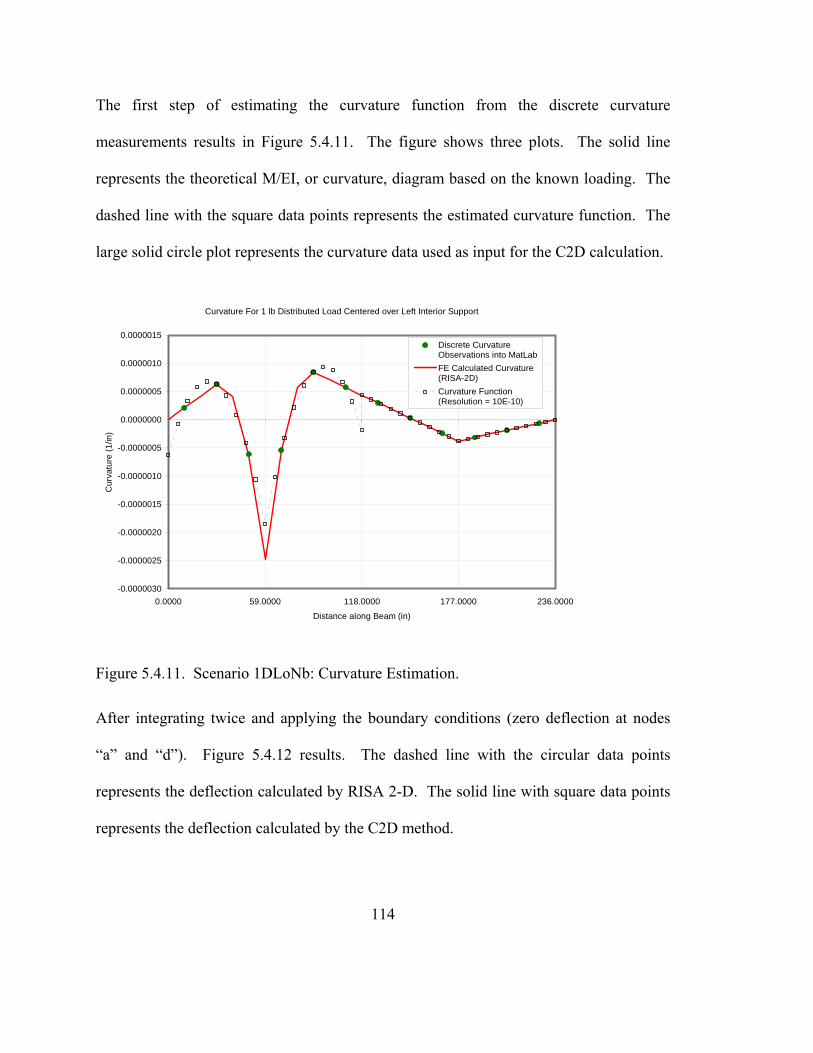
The first step of estimating the curvature function from the discrete curvature
measurements results in Figure 5.4.11. The figure shows three plots. The solid line
represents the theoretical M/EI, or curvature, diagram based on the known loading. The
dashed line with the square data points represents the estimated curvature function. The
large solid circle plot represents the curvature data used as input for the C2D calculation.
Curvature For 1 lb Distributed Load Centered over Left Interior Support
-0.0000030
-0.0000025
-0.0000020
-0.0000015
-0.0000010
-0.0000005
0.0000000
0.0000005
0.0000010
0.0000015
0.0000 59.0000 118.0000 177.0000 236.0000
Distance along Beam (in)
Cur
vatu
re (1
/in)
Discrete CurvatureObservations into MatLabFE Calculated Curvature(RISA-2D)Curvature Function(Resolution = 10E-10)
Figure 5.4.11. Scenario 1DLoNb: Curvature Estimation.
After integrating twice and applying the boundary conditions (zero deflection at nodes
“a” and “d”). Figure 5.4.12 results. The dashed line with the circular data points
represents the deflection calculated by RISA 2-D. The solid line with square data points
represents the deflection calculated by the C2D method.
114

Deflection For 1 lb Distributed Load Centered over Left Interior Support
-0.0008
-0.0007
-0.0006
-0.0005
-0.0004
-0.0003
-0.0002
-0.0001
0.0000
0.0001
0.0002
0 59 118 177 236
Distance along Beam (in)
Def
lect
ion
(in)
Deflection Function(Resolution = 10E-10)
RISA 2D Deflection
Figure 5.4.12. Scenario 1DLoNb: Deflection Comparison.
For this load condition, the C2D calculated functions deviate from both the theoretical
curvature and deflection on the left half of the beam. These deviations occur on the two
beam sections where the distributed load is applied within the beam section. The most
significant deviation occurs at the calculated deflection of the interior support. The
curvature and displacement functions of the two other beam sections—on the right half of
the beam—are well represented.
5.4.8 Small Scale Implimentation
A small scale three span continuous beam was constructed and instrumented. The
idealized computer model used in section 5.4 intends to represent this small scale
structure. Both the scale model and computer model were subjected to a regime of loads
115

116
along each of the spans. The scale model was instrumented with weld-on electrical
resistance strain gauges, Fabry-Perot fiber optic strain gauges, and LVDTs. A static
loading case and a dynamic loading case are presented here.
5.4.8.1 Static Test
The beam supports are pinned at the left end and roller support at each of the other
supports. The data was acquired at 100 readings per second. Six Fabry-Perot fiber optic
strain gauges were used. The strain gauges are located at the top fiber of the tube steel
beam within two of the four beam sections defined by the C2D method—half of the beam
is instrumented while it was symmetrically loaded. The observed strains were mirrored
about the center of the beam to perform the C2D method calculations. The neutral axis
was assumed to be at mid-depth of the beam.
The data was acquired while the beam was loaded to four levels of load and held at each
level for several seconds. The loads were applied at the middle of the center span similar
to theoretical scenario 1MoCS in section 5.4.3. The four point loads were 2 lb, 4 lb, 6 lb,
and 9.5 lb in magnitude. The recorded strains are shown in Figure 5.4.13.
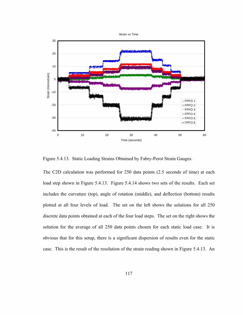
Strain vs Time
-40
-30
-20
-10
0
10
20
30
0 10 20 30 40 50 6
Time (seconds)
Stra
in (m
icro
stra
in)
0
FPFO 1FPFO 2FPFO 3FPFO 4FPFO 5FPFO 6
Figure 5.4.13. Static Loading Strains Obtained by Fabry-Perot Strain Gauges.
The C2D calculation was performed for 250 data points (2.5 seconds of time) at each
load step shown in Figure 5.4.13. Figure 5.4.14 shows two sets of the results. Each set
includes the curvature (top), angle of rotation (middle), and deflection (bottom) results
plotted at all four levels of load. The set on the left shows the solutions for all 250
discrete data points obtained at each of the four load steps. The set on the right shows the
solution for the average of all 250 data points chosen for each static load case. It is
obvious that for this setup, there is a significant dispersion of results even for the static
case. This is the result of the resolution of the strain reading shown in Figure 5.4.13. An
117
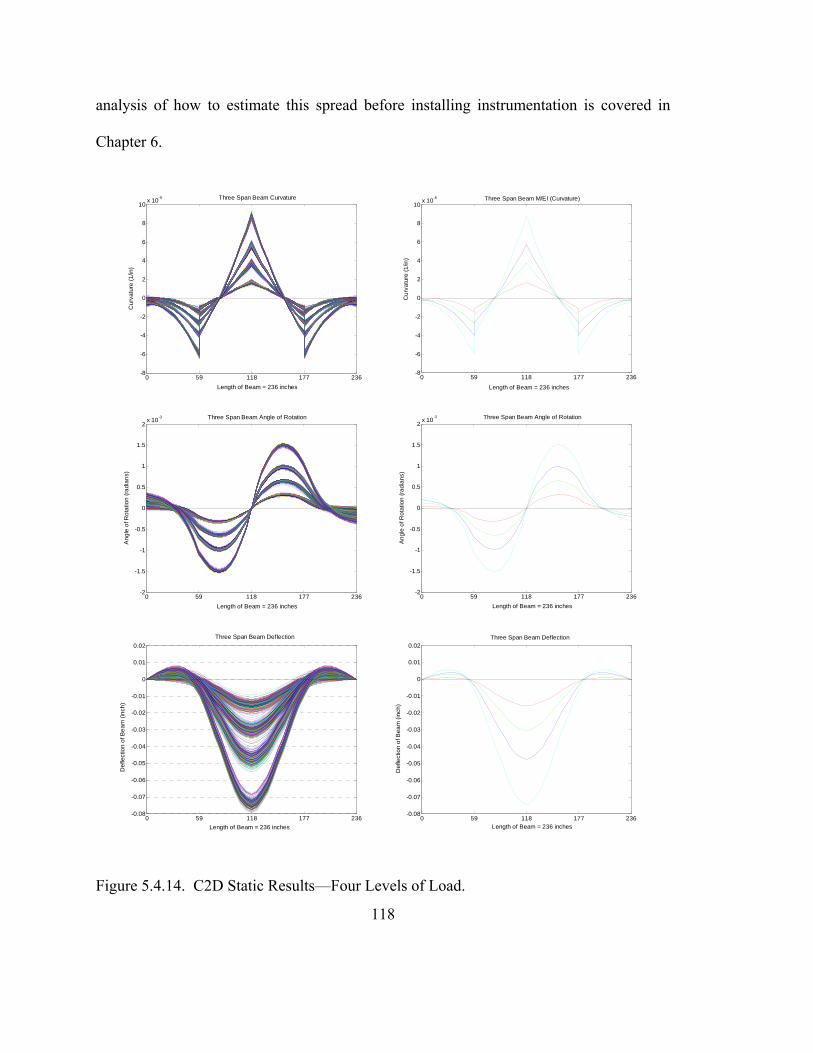
analysis of how to estimate this spread before installing instrumentation is covered in
Chapter 6.
0 59 118 177 236-2
-1.5
-1
-0.5
0
0.5
1
1.5
2x 10⁻³
Length of Beam = 236 inches
Ang
le o
f Rot
atio
n (ra
dian
s)
Three Span Beam Angle of Rotation
0 59 118 177 236-2
-1.5
-1
-0.5
0
0.5
1
1.5
2x 10⁻³
Length of Beam = 236 inches
Ang
le o
f Rot
atio
n (ra
dian
s)
Three Span Beam Angle of Rotation
0 59 118 177 236-8
-6
-4
-2
0
2
4
6
8
10x 10-5
Length of Beam = 236 inches
Cur
vatu
re (1
/in)
Three Span Beam Curvature
0 59 118 177 236-8
-6
-4
-2
0
2
4
6
8
10x 10-5
Length of Beam = 236 inches
Cur
vatu
re (1
/in)
Three Span Beam M/EI (Curvature)
0 59 118 177 236-0.08
-0.07
-0.06
-0.05
-0.04
-0.03
-0.02
-0.01
0
0.01
0.02
Length of Beam = 236 inches
Def
lect
ion
of B
eam
(inc
h)
Three Span Beam Deflection
0 59 118 177 236-0.08
-0.07
-0.06
-0.05
-0.04
-0.03
-0.02
-0.01
0
0.01
0.02
Def
lect
ion
of B
eam
(inc
h)
Three Span Beam Deflection
Length of Beam = 236 inches
Figure 5.4.14. C2D Static Results—Four Levels of Load.
118

119
5.4.8.2 Dynamic Tests
The small scale three-span beam was dynamically loaded by plucking the midpoint of the
center span. The beam was instrumented with 12 Fabry–Perot strain gauges located on
one half of the beam. They were arranged such that six curvature observations could be
made. Since the loading and boundary conditions are assumed to be symmetrical, the
acquired data was mirrored across the entire length of the system—all four beam
sections. The data was acquired at 200 readings per second. A single cycle (15 time
steps) of the free vibration was extracted to calculate the displaced shape of the beam by
the C2D method. The six obtained curvatures are shown in the top plot of Figure 5.4.15.
The C2D methodology was then applied to determine the curvature, angle of rotation,
and deflection functions of the beam. The results are shown in the lower three graphs of
Figure 5.4.15: curvature, angle of rotation, and deflection from left to right respectively.

Dynamic Curvature Readings
-0.000080
-0.000040
0.000000
0.000040
0.000080
0.000120
1 2 3 4 5 6 7 8 9 10 11 12 13 14 15
Time Step
Cur
vatu
re (r
adia
ns)
0 59 118 177 236-0.12
-0.06
0
0.06
0.12
Length of Beam = 236 inches
Def
lect
ion
of B
eam
(in)
0 59 118 177 236-2.5
-2
-1.5
-1
-0.5
0
0.5
1
1.5
2
2.5x 10⁻³
Length of Beam = 236 inches
Ang
le o
f Rot
atio
n (ra
dian
s)
0 59 118 177 236-1
-0.8
-0.6
-0.4
-0.2
0
0.2
0.4
0.6
0.8
1x 10⁻⁴
Length of Beam = 236 inches
Cur
vatu
re (1
/in)
Figure 5.4.15. C2D Method Observations, Dynamic Response of Small Scale Beam.
The results for the curvature are fairly consistent with the point loading applied to induce
the free vibration. However, some curvature plots that appear to have similar errors
observed in the theoretical static loading conditions; scenarios 1MoAS, 1QSoCS, and
1DLoNb described in section 5.4.2. Others [Aki & Robertson 2005] have shown that the
mode 1 dynamic deformed shape is obtained when excited by similar plucking. They
needed to perform some data “normalization” to force the deflection at the two interior
supports to zero [Aki & Robertson 2005]. Figure 5.4.16 shows the theoretical response
for mode 1 vibration that is scaled through a similar cycle of free vibration. Theoretically
calculated strains were linearly scaled to create 15 different states of strain to represent a
120
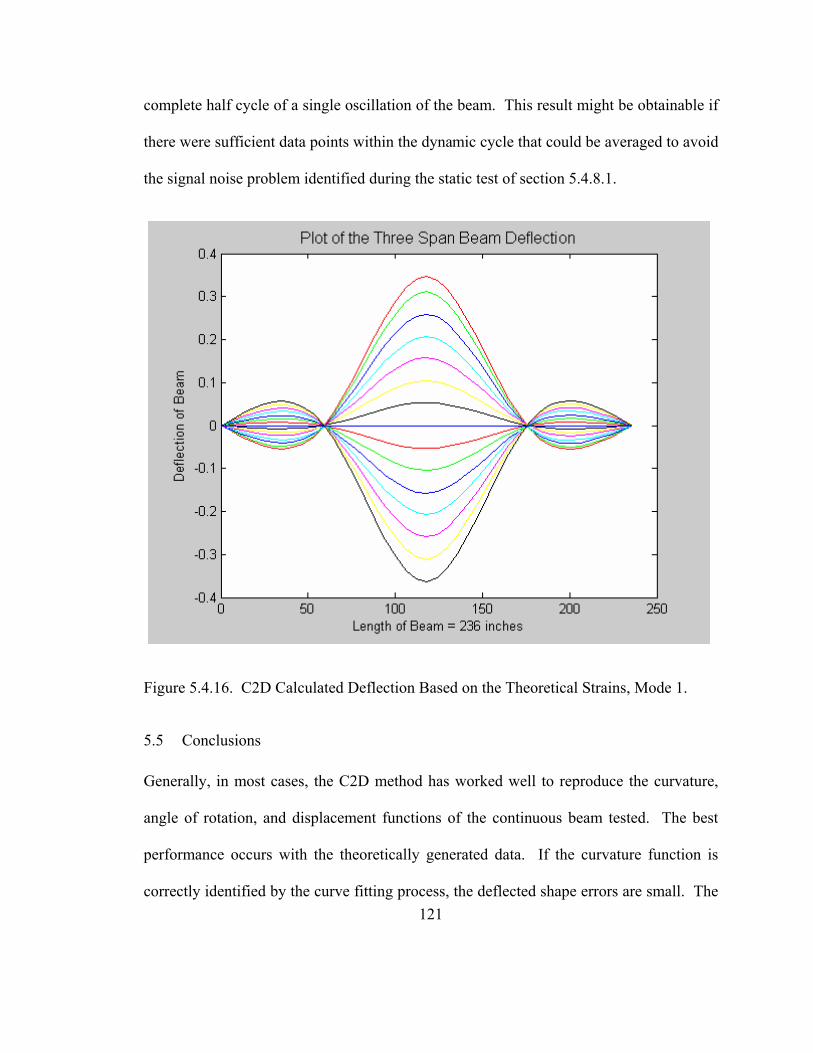
complete half cycle of a single oscillation of the beam. This result might be obtainable if
there were sufficient data points within the dynamic cycle that could be averaged to avoid
the signal noise problem identified during the static test of section 5.4.8.1.
Figure 5.4.16. C2D Calculated Deflection Based on the Theoretical Strains, Mode 1.
5.5 Conclusions
Generally, in most cases, the C2D method has worked well to reproduce the curvature,
angle of rotation, and displacement functions of the continuous beam tested. The best
performance occurs with the theoretically generated data. If the curvature function is
correctly identified by the curve fitting process, the deflected shape errors are small. The 121

122
use of data acquired from a real structure does not perform as well. The uncertainty of
the acquired curvature is likely the cause.
5.5.1 Comments on Curvature Estimation
The presented C2D method uses a second degree polynomial to estimate the curvature
function within each beam section. This estimate works well when the beam section is
loaded such that it satisfies the exact solution of the loading condition. However, when
the beam section is loaded by a point load within the beam section span, or partially
loaded with a distributed load, the second degree polynomial cannot replicate the real
curvature function. In the cases observed, this inability of the second degree polynomial
to replicate the curvature is limited to the beam sections where the non-conforming loads
occur—the curvature is well represented by the second degree polynomial at adjacent
beam sections. This is the advantage of a C1 continuous deflection solution—a
discontinuity of curvature is allowed at the node between beam sections. The C1
continuity only forces the displacement and angle of rotation function to be continuous.
5.5.2 Comments on Deflected Shape
The C2D method as implemented by the Matlab™ program assumes zero deflection at
the two end supports. The deflections at the two interior supports were not forced by
boundary conditions: they were calculated. The data used to generate the deflected
shapes can correctly identify the two interior support locations at the two internal zero
deflection nodes. However, in the theoretical loading scenario with a distributed load
partially loading two beam sections over the left interior support (1DLoNb), the C2D

123
result shows a non-zero displacement at that support. The general deflected shape was
still identified, but as with the other error-generating scenarios, this support error was
significantly larger than the support errors with different loading conditions. The errors
generated by loads that do not conform with the exact solutions best represented by a
second degree polynomial curvature function—or a fourth degree polynomial deflection
function—will require an alternate curvature function and requisite alternate number of
curvature measurement locations to obtain an exact solution.
5.5.3 Comments on Real Data Implementation
The real data acquired shows promise; however, there exists significant error beyond the
limitations identified by the theoretical loading scenarios. One example, in the small
scale implementation the C2D result shows non-zero displacement at the interior
supports. In other cases, the deflected shape is inconsistent with what is expected. The
static cases appear to perform better than the dynamic cases. This is likely due to the fact
that the static cases used averaged curvature as the input while the dynamic case used raw
data for a particular time step. Since the theoretical scenarios and its generated data work
quite well, these errors must be associated with measurement error. How the systematic
measurement error affects the C2D results will be discussed in Chapter 6.

124

125
CHAPTER 6. ANALYSIS OF STRAIN GAGE BASED DEFLECTED SHAPE
CALCULATIONS
6.1 Background
In chapter 5, we saw that by mechanics of materials, the slope of the normal strain
distribution through the depth of a beam at any section can be considered the curvature at
that section—assuming small deflections. Determining curvature from strain can provide
reasonable deflection estimates in some cases. The curvature to displacement (C2D)
Method (described in Chapter 5) utilizes fitting a function to observed curvatures and
applying appropriate boundary conditions to calculate an approximate deflected shape by
double integration.
In this type of deflection calculation, there are several practical issues to consider: where
to place the strain gauges that provide the curvature information; how many strain gauges
to use; and which strain measurement device to use.
Engineers will often want to observe events that are not approaching “design magnitude”
events. Typically to understand the system, an engineer and owner would much prefer to
test their structure in the elastic region subjected to service loads. The owner could also
wish to monitor “typical” events which may only cause a very small change in strain
within the structure. This could be a systematic problem that is difficult to overcome.
Some researchers have observed that smaller strain or load levels produce greater relative
error in the calculated deflection [Cho et al. 2000]. Others have noted that a minimum
precision in measuring strain is needed to reduce potential error [Vurpillot et al. 1998].

126
Some gauges are appropriate for some types of deflection measurements while others
may not be appropriate—an example would be performance observations of epoxy
bonded fiber optic strain gauges versus weldable electrical resistance strain gauges for
dynamic deflection measurements on a steel beam as noted by Aki and Robertson [2005].
This chapter discusses how real measurements—subject to systematic noise, limited
resolution, and digitization—can affect the C2D calculation results.
6.2 Error Sources in Real Data used in C2D Method
Measuring data using electronics have allowed us to increase the capacity to acquire
more information than ever before. However, there still exists a limit to the resolution of
these measurements. Two phenomena that can affect resolution of data acquired
electronically are the digitization process and the signal noise characteristics of the
transducer.
The digitization process translates a signal from a transducer/signal conditioner into a
binary number to be stored in the computer system. Since there is finite memory
available for storage, even an analog signal is truncated, or rounded off, at a resolution
consistent with the capabilities of the analog to digital converter (ADC) of the data
acquisition system. For example, if the ADC is a 12 bit device there is only enough
available processor capacity to store 212 (4096) distinct signal quantities. This means that
if the full range of the transducer is calibrated to measure +/- 5000 microstrain, the
smallest recordable difference in strain will be 2(5000)/4096 = 2.44 microstrain. This

127
resolution for the case of the C2D method may not be accurate enough to provide
acceptable results.
The signal noise characteristics of the transducer usually will provide the dominant
source of error in the C2D method algorithm. In most cases, transducers can be
calibrated into a data acquisition system such that the signal noise surpasses the
digitization round-off as the primary source of error. As described in previous chapters,
measurement devices are always subject to environmental phenomena that introduce
error into the signal observed by the data acquisition system. This noise limits the
resolution of the device. The C2D method can be greatly affected by these erroneous
observations.
6.2.1 Measurement Round Off
Measurement round off due to either signal digitization or post processing rounding of
data can greatly affect the output of the C2D method. In Chapter 5 five different loading
scenarios were used to observe how the C2D method performed as a tool to obtain the
deflected shape of a three-span continuous beam. The beam analyzed in that chapter had
a cross-sectional depth of 1 inch. The resolution of curvature used as input to the C2D
method algorithm was 10-10 inch-1. To achieve this resolution with real measurements it
would need to be instrumented with strain gauges that could observe changes of 0.0002
microstrain with stable readings at the top and bottom extreme fibers of the beam. This
type of system does not currently exist and / or would be too expensive to implement.
This effect of this resolution is that between four and five significant figures are used as

input data. A realistic goal for the measurement resolution of curvature to observe for the
beam setup used would be 1 microstrain. Rounding the data used in chapter 5 provides a
method to observe the effects of measurement round off in the C2D methodology. In this
section, all five cases observed in chapter 5 are repeated including the effects of rounding
to a resolution of 10-6 inch-1. Rounding to this level of resolution has the effect of
limiting the input data to one significant figure. The curvatures used as input for this
analysis are listed in Table 6.1.
Table 6.1. Curvature Input for Three Span Continuous Beam.
6.2.1.1 Matlab Implementation Scenario 1MoCS
This scenario represents a single unit load applied to the middle of the center span of the
structure represented in Figure 5.4.1. The curvature used in the C2D calculation is
reported in Table 6.1 above.
The first step of estimating the curvature function from the discrete curvature
measurements results in Figure 6.2.1. The figure shows four plots. The solid line
represents the theoretical M/EI, or curvature, diagram based on the known loading. The
dashed line with the square data points represents the estimated curvature function at the
10-10 inch-1 resolution. The large solid circle plot represents the curvature data used as
128

input for the C2D calculation before rounding. The heavy dashed line represents the
estimated curvature function obtained by the second-degree polynomial after rounding
the input curvature to the nearest 10-6 inch-1 resolution.
Curvature For Unit Point Load at Midspan of Center Span
-0.000008
-0.000006
-0.000004
-0.000002
0.000000
0.000002
0.000004
0.000006
0.000008
0.000010
0.000012
0 59 118 177 236
Distance along Beam (in)
Cur
vatu
re (1
/in)
Discrete CurvatureObservations into MatLab
FE Calculated Curvature(RISA-2D)
Curvature Function(Resolution = 10E-10)
Curvature Function(Resolution = 10E-6)
Figure 6.2.1. Scenario 1MoCS: C2D Curvature Comparison.
After integrating twice and applying the boundary conditions (zero deflection at nodes
“a” and “d”). Figure 6.2.2 results. The dashed line with the circular data points
represents the deflection calculated by RISA 2-D. The solid line with square data points
represents the deflection calculated by the C2D method before round off. The solid line
with triangular data points represents the deflection by the C2D method after round off.
129
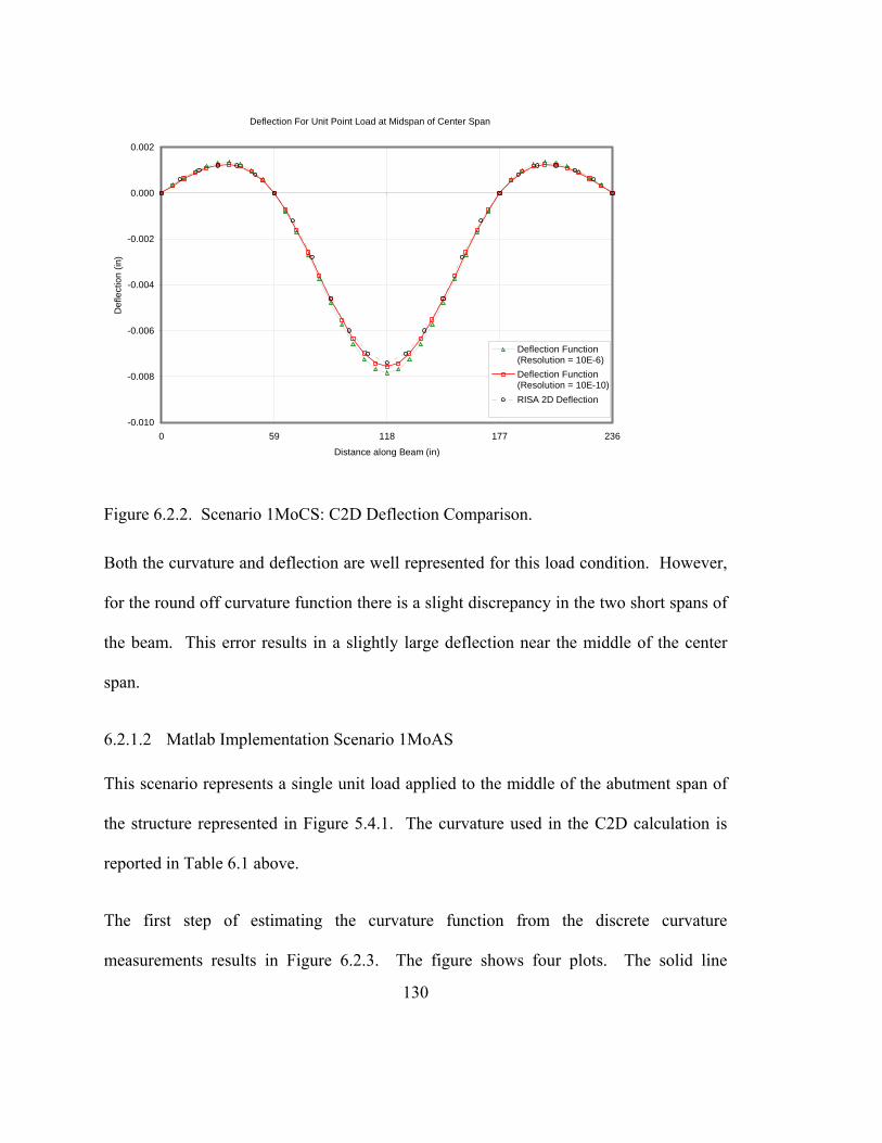
Deflection For Unit Point Load at Midspan of Center Span
-0.010
-0.008
-0.006
-0.004
-0.002
0.000
0.002
0 59 118 177 236
Distance along Beam (in)
Def
lect
ion
(in)
Deflection Function(Resolution = 10E-6)Deflection Function(Resolution = 10E-10)RISA 2D Deflection
Figure 6.2.2. Scenario 1MoCS: C2D Deflection Comparison.
Both the curvature and deflection are well represented for this load condition. However,
for the round off curvature function there is a slight discrepancy in the two short spans of
the beam. This error results in a slightly large deflection near the middle of the center
span.
6.2.1.2 Matlab Implementation Scenario 1MoAS
This scenario represents a single unit load applied to the middle of the abutment span of
the structure represented in Figure 5.4.1. The curvature used in the C2D calculation is
reported in Table 6.1 above.
The first step of estimating the curvature function from the discrete curvature
measurements results in Figure 6.2.3. The figure shows four plots. The solid line
130

represents the theoretical M/EI, or curvature, diagram based on the known loading. The
dashed line with the square data points represents the estimated curvature function at the
10-10 inch-1 resolution. The large solid circle plot represents the curvature data used as
input for the C2D calculation before rounding. The heavy dashed line represents the
estimated curvature function obtained by the second-degree polynomial after rounding
the input curvature to the nearest 10-6 inch-1 resolution.
Curvature For Unit Point Load at Midspan of Abutment Span
-0.000008
-0.000006
-0.000004
-0.000002
0.000000
0.000002
0.000004
0.000006
0.000008
0 59 118 177 236
Distance along Beam (in)
Cur
vatu
re (1
/in)
Discrete CurvatureObservations into MatLabFE Calculated Curvature(RISA-2D)Curvature Function(Resolution = 10E-10)Curvature Function(Resolution = 10E-6)
Figure 6.2.3. Scenario 1MoAS: C2D Curvature Comparison.
After integrating twice and applying the boundary conditions (zero deflection at nodes
“a” and “d”). Figure 6.2.4 results. The dashed line with the circular data points
represents the deflection calculated by RISA 2-D. The solid line with square data points
131

represents the deflection calculated by the C2D method before round off. The solid line
with triangular data points represents the deflection by the C2D method after round off.
Deflection For Unit Point Load at Midspan of Abutment Span
-0.0025
-0.0020
-0.0015
-0.0010
-0.0005
0.0000
0.0005
0.0010
0.0015
0.0020
0 59 118 177 236
Distance along Beam (in)
Def
lect
ion
(in)
Deflection Function(Resolution = 10E-6)Deflection Function(Resolution = 10E-10)RISA 2D Deflection
Figure 6.2.4. Scenario 1MoAS: C2D Deflection Comparison.
Prior to rounding, the C2D calculated functions significantly deviate from both the
theoretical curvature and deflection within the left abutment span where the point load is
applied within the beam section. Before rounding, the curvature and displacement
functions of the three other beam sections are well represented. However, after rounding
the curvature function misrepresents the theoretical curvature at all four beam sections.
Also, after rounding, the deflection calculated by the C2D method significantly deviates
from the theoretical deflection curve at the two beam sections within the central span.
132

133
6.2.1.3 Matlab Implementation Scenario 1QPoCS
This scenario represents a single unit load applied to the left quarter point of the center
span of the structure represented in Figure 5.4.1. The curvature used in the C2D
calculation is reported in Table 6.1 above.
The first step of estimating the curvature function from the discrete curvature
measurements results in Figure 6.2.5. The figure shows four plots. The solid line
represents the theoretical M/EI, or curvature, diagram based on the known loading. The
dashed line with the square data points represents the estimated curvature function at the
10-10 inch-1 resolution. The large solid circle plot represents the curvature data used as
input for the C2D calculation before rounding. The heavy dashed line represents the
estimated curvature function obtained by the second-degree polynomial after rounding
the input curvature to the nearest 10-6 inch-1 resolution.

Curvature For Unit Point Load at Quarter Point of Center Span
-0.000012
-0.000010
-0.000008
-0.000006
-0.000004
-0.000002
0.000000
0.000002
0.000004
0.000006
0.000008
0 59 118 177 236
Distance along Beam (in)
Cur
vatu
re (1
/in)
Discrete CurvatureObservations into MatLabFE Calculated Curvature(RISA-2D)Curvature Function(Resolution = 10E-10)Curvature Function(Resolution = 10E-6)
Figure 6.2.5. Scenario 1QPoCS: C2D Curvature Comparison.
After integrating twice and applying the boundary conditions (zero deflection at nodes
“a” and “d”). Figure 6.2.6 results. The dashed line with the circular data points
represents the deflection calculated by RISA 2-D. The solid line with square data points
represents the deflection calculated by the C2D method before round off. The solid line
with triangular data points represents the deflection by the C2D method after round off.
134
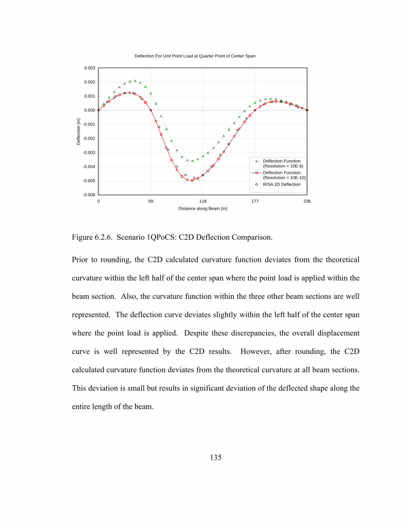
Deflection For Unit Point Load at Quarter Point of Center Span
-0.006
-0.005
-0.004
-0.003
-0.002
-0.001
0.000
0.001
0.002
0.003
0 59 118 177 236
Distance along Beam (in)
Def
lect
ion
(in)
Deflection Function(Resolution = 10E-6)Deflection Function(Resolution = 10E-10)RISA 2D Deflection
Figure 6.2.6. Scenario 1QPoCS: C2D Deflection Comparison.
Prior to rounding, the C2D calculated curvature function deviates from the theoretical
curvature within the left half of the center span where the point load is applied within the
beam section. Also, the curvature function within the three other beam sections are well
represented. The deflection curve deviates slightly within the left half of the center span
where the point load is applied. Despite these discrepancies, the overall displacement
curve is well represented by the C2D results. However, after rounding, the C2D
calculated curvature function deviates from the theoretical curvature at all beam sections.
This deviation is small but results in significant deviation of the deflected shape along the
entire length of the beam.
135

136
6.2.1.4 Matlab Implementation Scenario 1DLoM2
This scenario represents a uniformly distributed load totaling one pound applied to the
left half of the center span of the structure represented in Figure 5.4.1. The curvature
used in the C2D calculation is reported in Table 6.1 above.
The first step of estimating the curvature function from the discrete curvature
measurements results in Figure 6.2.7. The figure shows four plots. The solid line
represents the theoretical M/EI, or curvature, diagram based on the known loading. The
dashed line with the square data points represents the estimated curvature function at the
10-10 inch-1 resolution. The large solid circle plot represents the curvature data used as
input for the C2D calculation before rounding. The heavy dashed line represents the
estimated curvature function obtained by the second-degree polynomial after rounding
the input curvature to the nearest 10-6 inch-1 resolution.
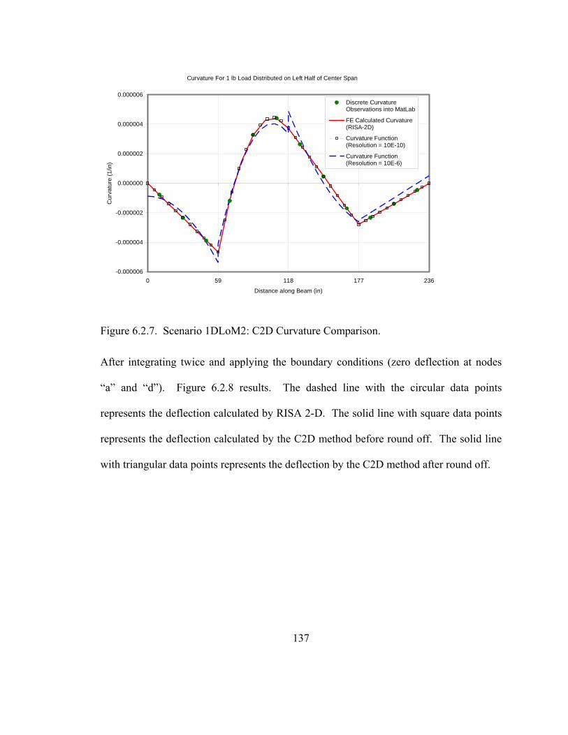
Curvature For 1 lb Load Distributed on Left Half of Center Span
-0.000006
-0.000004
-0.000002
0.000000
0.000002
0.000004
0.000006
0 59 118 177 236
Distance along Beam (in)
Cur
vatu
re (1
/in)
Discrete CurvatureObservations into MatLab
FE Calculated Curvature(RISA-2D)
Curvature Function(Resolution = 10E-10)
Curvature Function(Resolution = 10E-6)
Figure 6.2.7. Scenario 1DLoM2: C2D Curvature Comparison.
After integrating twice and applying the boundary conditions (zero deflection at nodes
“a” and “d”). Figure 6.2.8 results. The dashed line with the circular data points
represents the deflection calculated by RISA 2-D. The solid line with square data points
represents the deflection calculated by the C2D method before round off. The solid line
with triangular data points represents the deflection by the C2D method after round off.
137
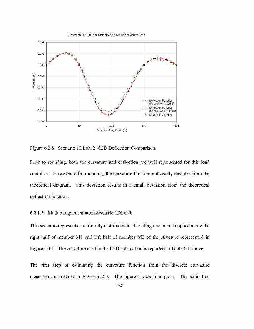
Deflection For 1 lb Load Distributed on Left Half of Center Span
-0.005
-0.004
-0.003
-0.002
-0.001
0.000
0.001
0.002
0 59 118 177 236
Distance along Beam (in)
Def
lect
ion
(in)
Deflection Function(Resolution = 10E-6)Deflection Function(Resolution = 10E-10)RISA 2D Deflection
Figure 6.2.8. Scenario 1DLoM2: C2D Deflection Comparison.
Prior to rounding, both the curvature and deflection are well represented for this load
condition. However, after rounding, the curvature function noticeably deviates from the
theoretical diagram. This deviation results in a small deviation from the theoretical
deflection function.
6.2.1.5 Matlab Implementation Scenario 1DLoNb
This scenario represents a uniformly distributed load totaling one pound applied along the
right half of member M1 and left half of member M2 of the structure represented in
Figure 5.4.1. The curvature used in the C2D calculation is reported in Table 6.1 above.
The first step of estimating the curvature function from the discrete curvature
measurements results in Figure 6.2.9. The figure shows four plots. The solid line
138

represents the theoretical M/EI, or curvature, diagram based on the known loading. The
dashed line with the square data points represents the estimated curvature function at the
10-10 inch-1 resolution. The large solid circle plot represents the curvature data used as
input for the C2D calculation before rounding. The heavy dashed line represents the
estimated curvature function obtained by the second-degree polynomial after rounding
the input curvature to the nearest 10-6 inch-1 resolution.
Curvature For 1 lb Distributed Load Centered over Left Interior Support
-0.0000035
-0.0000030
-0.0000025
-0.0000020
-0.0000015
-0.0000010
-0.0000005
0.0000000
0.0000005
0.0000010
0.0000015
0 59 118 177 236
Distance along Beam (in)
Cur
vatu
re (1
/in)
Discrete CurvatureObservations into MatLab
FE Calculated Curvature(RISA-2D)
Curvature Function(Resolution = 10E-10)
Curvature Function(Resolution = 10E-6)
Figure 6.2.9. Scenario 1DLoNb: C2D Curvature Comparison.
After integrating twice and applying the boundary conditions (zero deflection at nodes
“a” and “d”). Figure 6.2.10 results. The dashed line with the circular data points
represents the deflection calculated by RISA 2-D. The solid line with square data points
139

represents the deflection calculated by the C2D method before round off. The solid line
with triangular data points represents the deflection by the C2D method after round off.
Deflection For 1 lb Distributed Load Centered over Left Interior Support
-0.0010
-0.0008
-0.0006
-0.0004
-0.0002
0.0000
0.0002
0.0004
0 59 118 177 236
Distance along Beam (in)
Def
lect
ion
(in)
Deflection Function(Resolution = 10E-6)Deflection Function(Resolution = 10E-10)RISA 2D Deflection
Figure 6.2.10. Scenario 1DLoNb: C2D Deflection Comparison.
Prior to rounding, the C2D calculated functions deviate from both the theoretical
curvature and deflection on the left half of the beam. These deviations occur on the two
beam sections where the distributed load is applied within the beam section. The most
significant deviation occurs at the calculated deflection of the interior support. The
curvature and displacement functions of the two other beam sections—on the right half of
the beam—are well represented. There is significant deviation from both the theoretical
curvature and deflection functions after averaging occurs. The largest deviation occurs at
a location that is far from the applied load.
140

141
6.2.2 Signal Noise Characteristics
The purpose of this section is to show that signal noise characterization is important to
determining the type and placement of strain gauges used to observe curvature in the
C2D methodology. Signal noise characterization can also provide a tool to simulate the
effect of real noise on theoretical data sets. To determine the sensitivity of a
mathematical model to noise within a signal, both the signal and noise must first be
classified. Signals can be classified by morphological, phenomenological, energy, and
spectral criteria [Zepernick & Finger 2005, pg 7]. This section will show one such
example based on Fabry-Perot strain gauge data observed on the three-span continuous
beam described earlier in this chapter and defined in chapter 5.
Morphological classification describes the form of the signal as continuous or discrete.
The classification considers that both the time and the signal could be either continuous
or discrete. There are four possible combinations of these morphologic signal
characteristics. Each combination dictates how to handle the analysis and representation
of the signal. It is obvious that the data collected to monitor structures are a discrete time
based signal. Even during seismic events—when an analogue signal would be
preferable—an acceleration time history would be sampled at a frequency on the order of
200 Hz. It is less intuitive, however, that the signal value is also a discrete form of data.
The phenomenon is usually measured by an analogue device, but its signal becomes
digital by two potential limiting factors: the minimum detectable change within the signal
conditioner (often the smallest voltage change) and the digitization limits of the analogue
to digital converter (ADC) used to allow a computer to store the data points. To better

142
understand these limiting factors, consider measuring a rod with a ruler marked to every
1 cm. Let the actual length of the rod be 3.25 cm; this represents an analogue signal. By
standard scientific practice, the closest detectable values that are observable, per an error
of measure of 0.5 cm, would be either 3 cm or 3.5 cm. This is analogous to digital round
off error due to the detection limits of the signal conditioner. Now, if the required format
of recording the rod length only allows for eight possible values for a range from 0 cm to
10 cm the recorded length would be either 2.9 cm or 4.3 cm. This is analogous to an
ADC imposed rounding error. Strain based data has a morphological classification of
discrete-time and discrete-value signal. Typically, these signals will also be aperiodic.
Section 6.2.1 adequately demonstrates the possible effects of this classification on the
C2D methodology.
Phenomenological classification describes whether the data is deterministic or random.
Deterministic signals can be described by mathematical expressions. Examples would be
the Dirac impulse, sine waves, et cetera. A random signal could be described by
probabilities, probability distributions, probability densities, averages, et cetera. The data
for strain measurements are deterministic with random characteristics. A signal of this
type of data is also known as a pseudo random signal. Rather than performing a full
criteria check that this data meets the pseudo random signal criteria, it was assumed
based on the general definition of pseudo random signals that strain gauge data met all
the criteria described by Zepernick & Finger [2005].
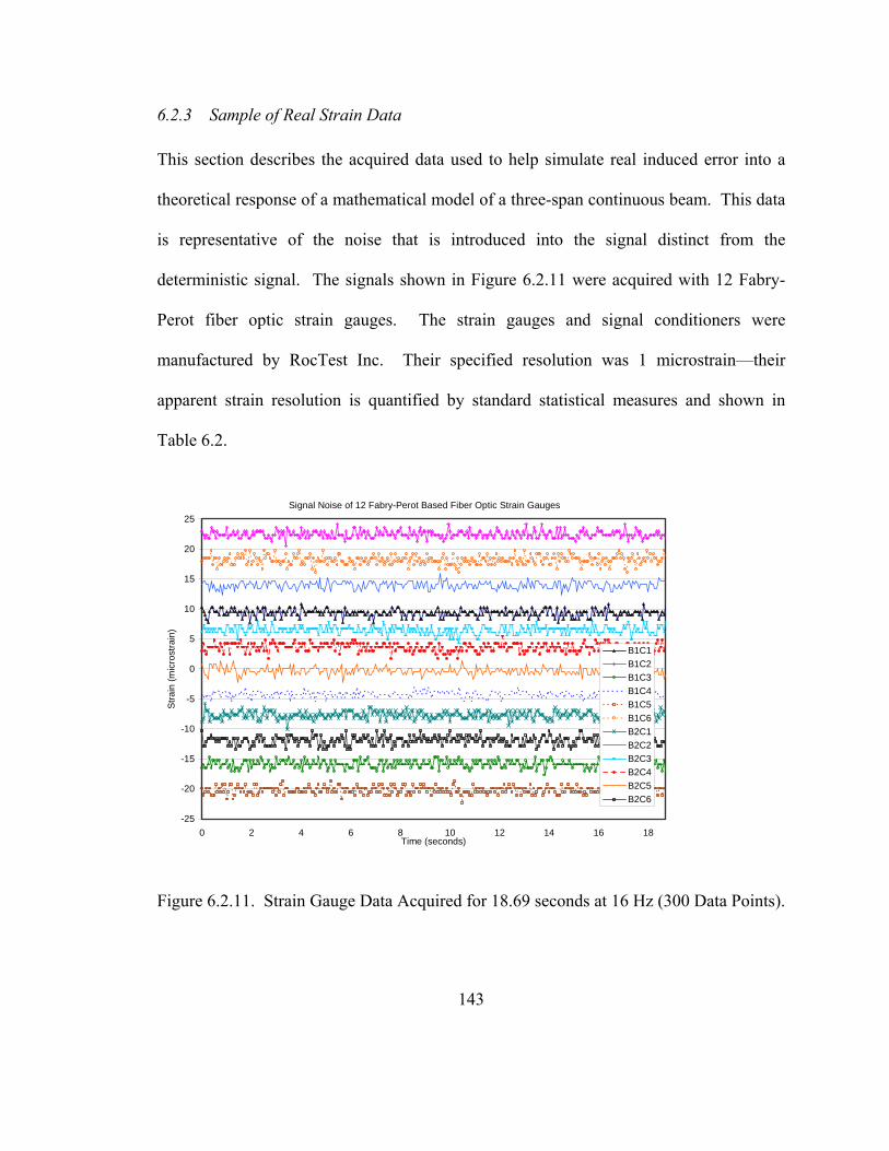
6.2.3 Sample of Real Strain Data
This section describes the acquired data used to help simulate real induced error into a
theoretical response of a mathematical model of a three-span continuous beam. This data
is representative of the noise that is introduced into the signal distinct from the
deterministic signal. The signals shown in Figure 6.2.11 were acquired with 12 Fabry-
Perot fiber optic strain gauges. The strain gauges and signal conditioners were
manufactured by RocTest Inc. Their specified resolution was 1 microstrain—their
apparent strain resolution is quantified by standard statistical measures and shown in
Table 6.2.
Signal Noise of 12 Fabry-Perot Based Fiber Optic Strain Gauges
-25
-20
-15
-10
-5
0
5
10
15
20
25
0 2 4 6 8 10 12 14 16 18Time (seconds)
Stra
in (m
icro
stra
in)
B1C1B1C2B1C3B1C4B1C5B1C6B2C1B2C2B2C3B2C4B2C5B2C6
Figure 6.2.11. Strain Gauge Data Acquired for 18.69 seconds at 16 Hz (300 Data Points).
143

Table 6.2. Statistical Characteristics of Strain Error Based on Average Strain Value.
6.3 Analysis of Error Propagation in C2D Method
In this section the propagation of error is analyzed. Primarily, signal noise will be
discussed; the propagation of round off error has been demonstrated in section 6.2.1. In
most cases, round off error will occur when a static loading condition is observed and
many readings are averaged. If the result of the averaging is not carried to enough digits,
round off error might cause problems. In dynamic loading, or continuous data sets,
signal noise will generally be larger than the round off error. During the following
analysis, different assumed magnitudes of error are applied to theoretical data to observe
the effect how the C2D methodology results are affected. In some cases, real data with
its natural error will be compared to the theoretically generated error modified data.
First, observations of the effects of error at an individual sensor are shown. The error
affects the beam section where the error occurs as well as the entire length of the beam.
Second, observations of the effects of error at multiple sensors are shown. Errors at
different sensors may combine to increase the overall error, or errors at multiple sensors
may counteract each other in some places and increase the error in others.
144

145
6.3.1 Error at Individual Sensors
In section 6.2.3 we saw some examples of real strain data. The standard deviation of the
noise fluctuation for each gauge type ranged from 0.7 microstrain to 3 microstrain. If this
is a random error occurrence, the maximum expected error magnitude could be +/-1
microstrain to +/-5 microstrain. A two microstrain error corresponds to a 10-6 inch-1
curvature error. The effect of a 10-6 inch-1 error at an individual curvature location has
been applied to a single beam section. A 10-6 inch-1 error has also been applied to one
sensor along the full length of the three-span small scale beam as well. These maximum
likely strain errors can be scaled to account for any expected signal error of a strain gauge
technology.
6.3.1.1 Single Beam Section
The typical beam section of the system in Figure 5.4.1 has three curvature measurements.
Assume that a 10-6 inch-1 error of curvature occurs at one of the three locations. In that
beam section, there are three possible sets of curvature, rotation and deflection curves
generated by the C2D method. Figure 6.3.1 shows the three curvature functions that are
produced by a second degree polynomial. Note that the x-axis represents zero error along
the length of the beam section. The rotation and deflection functions are based on zero
rotation and zero deflection at the left support—cantilever beam. The functions are
shown in Figure 6.3.2 and Figure 6.3.3, respectively. Again, with no error, both the
rotation and deflection curves would be zero along the entire length of the beam section.
The plots represent the error that propagates from a single erroneous curvature
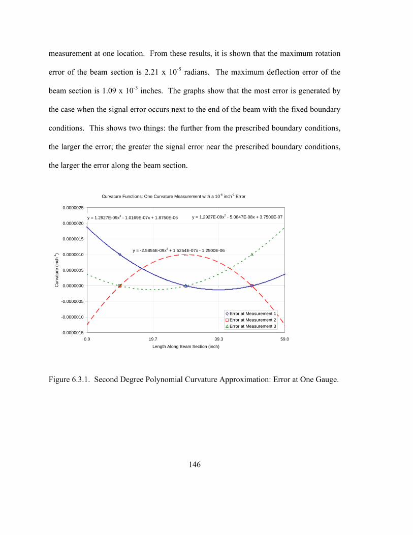
measurement at one location. From these results, it is shown that the maximum rotation
error of the beam section is 2.21 x 10⁻⁵ radians. The maximum deflection error of the
beam section is 1.09 x 10⁻³ inches. The graphs show that the most error is generated by
the case when the signal error occurs next to the end of the beam with the fixed boundary
conditions. This shows two things: the further from the prescribed boundary conditions,
the larger the error; the greater the signal error near the prescribed boundary conditions,
the larger the error along the beam section.
Curvature Functions: One Curvature Measurement with a 10-6 inch-1 Error
y = 1.2927E-09x2 - 1.0169E-07x + 1.8750E-06
y = -2.5855E-09x2 + 1.5254E-07x - 1.2500E-06
y = 1.2927E-09x2 - 5.0847E-08x + 3.7500E-07
-0.0000015
-0.0000010
-0.0000005
0.0000000
0.0000005
0.0000010
0.0000015
0.0000020
0.0000025
0.0 19.7 39.3 59.0
Length Along Beam Section (inch)
Cur
vatu
re (i
nch-1
)
Error at Measurement 1Error at Measurement 2Error at Measurement 3
Figure 6.3.1. Second Degree Polynomial Curvature Approximation: Error at One Gauge.
146
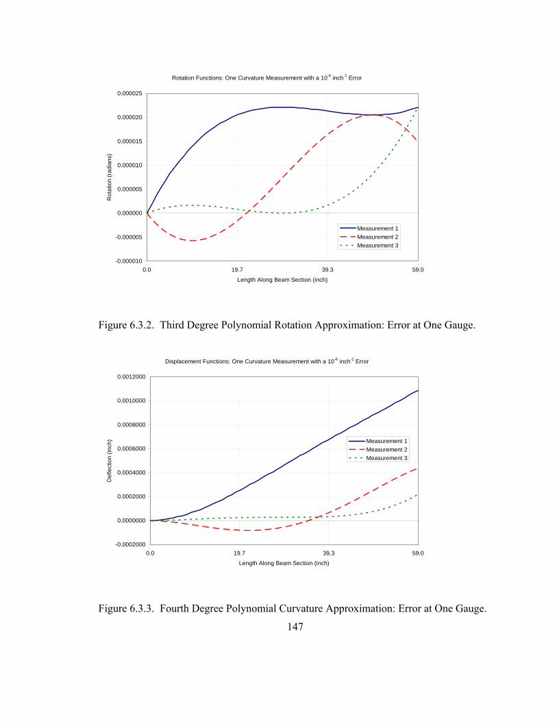
Rotation Functions: One Curvature Measurement with a 10-6 inch-1 Error
-0.000010
-0.000005
0.000000
0.000005
0.000010
0.000015
0.000020
0.000025
0.0 19.7 39.3 59.0
Length Along Beam Section (inch)
Rot
atio
n (r
adia
ns)
Measurement 1Measurement 2Measurement 3
Figure 6.3.2. Third Degree Polynomial Rotation Approximation: Error at One Gauge.
Displacement Functions: One Curvature Measurement with a 10-6 inch-1 Error
-0.0002000
0.0000000
0.0002000
0.0004000
0.0006000
0.0008000
0.0010000
0.0012000
0.0 19.7 39.3 59.0
Length Along Beam Section (inch)
Def
lect
ion
(inch
) Measurement 1Measurement 2Measurement 3
Figure 6.3.3. Fourth Degree Polynomial Curvature Approximation: Error at One Gauge.
147

148
6.3.1.2 Entire Beam
The previous section shows how the error at a single curvature measurement can
propagate through a single beam section. Generally, as the location along the axis of the
beam section is further from the prescribed boundary conditions, the larger the error. In
the previous case, the error exists at an end of the beam section. Since the formulation of
the C2D method ensures C1 continuity of the deflection curve, the error at the end of one
beam section becomes the boundary condition of the next beam section. This is
demonstrated in this section. The structural system analyzed in the three-span continuous
beam is shown in Chapter 5.
The C2D idealized beam uses four beam sections with three curvature measurement
locations. This system is analyzed in a similar manor as the previous section, however,
the global boundary conditions prescribe that the deflection at the ends of the beam are
zero. Assuming a 10-6 inch-1 error of curvature occurring at one of the 12 locations
generates the 12 possible plots in the curvature, rotation and deflection functions in
Figure 6.3.4, Figure 6.3.5, and Figure 6.3.6 respectively.
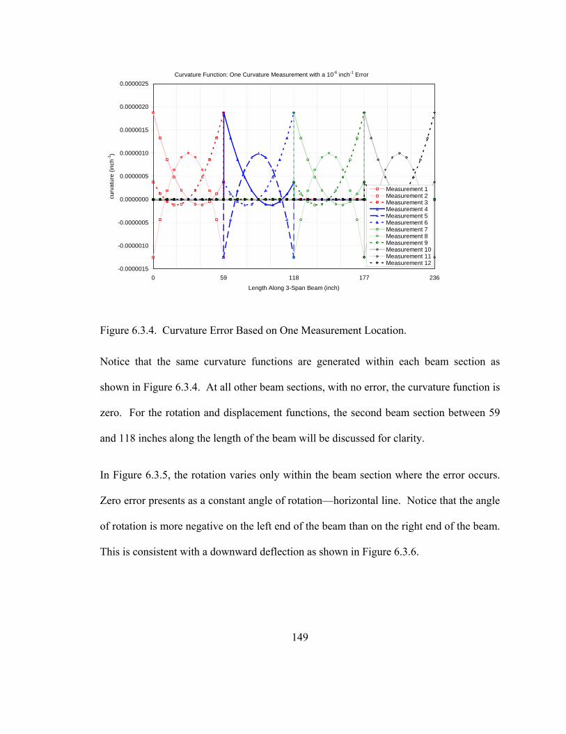
Curvature Function: One Curvature Measurement with a 10-6 inch-1 Error
-0.0000015
-0.0000010
-0.0000005
0.0000000
0.0000005
0.0000010
0.0000015
0.0000020
0.0000025
0 59 118 177 236
Length Along 3-Span Beam (inch)
curv
atur
e (in
ch-1
)
Measurement 1Measurement 2Measurement 3Measurement 4Measurement 5Measurement 6Measurement 7Measurement 8Measurement 9Measurement 10Measurement 11Measurement 12
Figure 6.3.4. Curvature Error Based on One Measurement Location.
Notice that the same curvature functions are generated within each beam section as
shown in Figure 6.3.4. At all other beam sections, with no error, the curvature function is
zero. For the rotation and displacement functions, the second beam section between 59
and 118 inches along the length of the beam will be discussed for clarity.
In Figure 6.3.5, the rotation varies only within the beam section where the error occurs.
Zero error presents as a constant angle of rotation—horizontal line. Notice that the angle
of rotation is more negative on the left end of the beam than on the right end of the beam.
This is consistent with a downward deflection as shown in Figure 6.3.6.
149
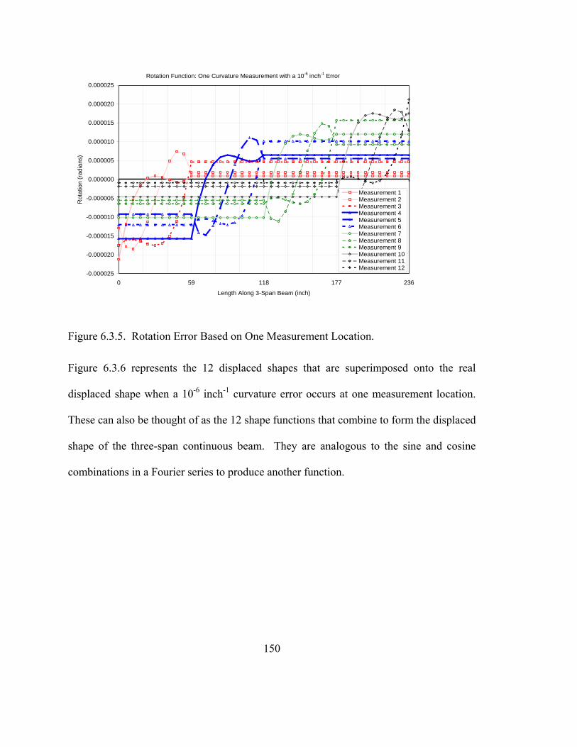
Rotation Function: One Curvature Measurement with a 10-6 inch-1 Error
-0.000025
-0.000020
-0.000015
-0.000010
-0.000005
0.000000
0.000005
0.000010
0.000015
0.000020
0.000025
0 59 118 177 236
Length Along 3-Span Beam (inch)
Rot
atio
n (r
adia
ns)
Measurement 1Measurement 2Measurement 3Measurement 4Measurement 5Measurement 6Measurement 7Measurement 8Measurement 9Measurement 10Measurement 11Measurement 12
Figure 6.3.5. Rotation Error Based on One Measurement Location.
Figure 6.3.6 represents the 12 displaced shapes that are superimposed onto the real
displaced shape when a 10-6 inch-1 curvature error occurs at one measurement location.
These can also be thought of as the 12 shape functions that combine to form the displaced
shape of the three-span continuous beam. They are analogous to the sine and cosine
combinations in a Fourier series to produce another function.
150

Deflection Function: One Curvature Measurement with a 10-6 inch-1 Error
-0.0016
-0.0014
-0.0012
-0.001
-0.0008
-0.0006
-0.0004
-0.0002
0
0 59 118 177 236
Length Along 3-Span Beam (inch)
Dis
plac
emen
t (in
ch)
Measurement 1Measurement 2Measurement 3Measurement 4Measurement 5Measurement 6Measurement 7Measurement 8Measurement 9Measurement 10Measurement 11Measurement 12
Figure 6.3.6. Displacement Error Based on One Measurement Location.
The displacement functions in Figure 6.3.6 can be combined by superposition to show the
magnitude of error due to any combination of errors at any combination of measurement
locations for a C2D modeled beam. The figure shows that the largest error occurs away
from the specified boundary conditions. In this example, the two boundary conditions
that control are zero displacement at zero and 236 inches along the length of the beam.
6.3.2 Error at Multiple Sensors
In section 6.3.1, error in the estimated curvature, angle of rotation, and displaced shapes
due to a single erroneous measurement were considered. Unfortunately, every
measurement of curvature used for the C2D method will introduce its own magnitude and
direction of error into the system. Each error will affect the entire length of the modeled
151

152
beam. The last section has provided us with a tool to estimate the maximum expected
error within the C2D beam model. In this section, the use of this tool will be
demonstrated using superposition of the results, obtained in section 6.3.1, as applied to
several measurement locations. The outcome will be compared to real data from the
small scale model as tested in the Materials Testing Laboratory at the University of
Hawaii. The C2D method will produce results which show the entire deflected shape of
the beam as well as for single locations measured by devices such as LVDTs.
6.3.2.1 Deflected Shape of the Entire Beam
In the entire length of a beam, multiple errors will occur. The errors will occur
simultaneously. To analyze the effect of these multiple errors, in a general sense, it can
be assumed that the errors will be of unit magnitude (10-6 inch-1). The errors can be
incorporated into the C2D method to see what effect it has on the deflected shape. To
get an idea of how the resulting displaced shapes combine when the error occurs at
multiple locations, several cases were manually combined by superposition. In section,
6.3.1, unit errors were applied at individual locations, the error in one direction or the
other caused the same magnitude of error displacement. However, during a real data
acquisition process, signal noise will generate positive and negative measurement errors.
Table 6.3 shows eight different combinations of unit error applied as a positive unit
curvature at various locations. The combinations were chosen to represent a large range
of possible error combinations. Table 6.4 shows eight different combinations of unit
error applied in either the positive or negative curvature direction. The combinations
chosen in Table 6.4 represent the variability in positive and negative error from one

measurement location to the next. At the top of the table, the error alternates direction at
each adjacent measurement location, and at the bottom of the table, half the beam has a
positive unit error and half has a negative unit error.
Table 6.3. Positive Error Combinations Calculated by Superposition.
Table 6.4. Alternating Direction Error Combinations Calculated by Superposition.
Figure 6.3.7 shows eight iterations of error that act in the positive curvature direction as
they affect the deflection function along the three-span small scale beam. The deflections
are calculated by superposition from the results shown in Figure 6.3.6—these results are
re-plotted in light gray in Figure 6.3.7 for comparison. The first two combinations are
errors that occur at locations 1 and 7 and at locations 3 and 9. These combinations show
that when at least one of the errors occurs near the specified boundary conditions, the
153

error will not be significantly magnified. The third and fourth combinations show the
effect of three errors occurring at adjacent measurement locations. When the errors occur
further from a specified boundary condition, the error is greater. The fifth combination is
a sum of the third and fourth combination. This combination shows a clear
representation of the superposition principle in action—it is clearly seen that the fifth is
the sum of three and four. The sixth and seventh combinations show the deflected shape
with unit errors at all the measurement locations except for one. When comparing these
two deflected shapes with the eighth combination, again, it is obvious that the error
occurring at the furthest position away from a specified boundary condition makes the
biggest difference in the overall error within the deflected shape.
Deflection Function: Multiple Curvature Measurements Locations with a 10-6 inch-1 Error
-0.008
-0.007
-0.006
-0.005
-0.004
-0.003
-0.002
-0.001
0
0.001
0.002
0 59 118 177 236
Length Along 3-Span Beam (inch)
Dis
plac
emen
t (in
ch)
At Locations 1 and 7At Locations 3 and 9At Locations 1, 2, and 3At Locations 4, 5, and 6At Locations 1 through 6All Locations but 6All Locations but 12All Locations
Figure 6.3.7. Deflection Based on Multiple Positive Curvature Error Locations.
154
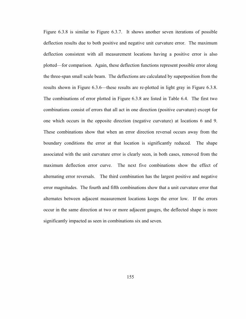
155
Figure 6.3.8 is similar to Figure 6.3.7. It shows another seven iterations of possible
deflection results due to both positive and negative unit curvature error. The maximum
deflection consistent with all measurement locations having a positive error is also
plotted—for comparison. Again, these deflection functions represent possible error along
the three-span small scale beam. The deflections are calculated by superposition from the
results shown in Figure 6.3.6—these results are re-plotted in light gray in Figure 6.3.8.
The combinations of error plotted in Figure 6.3.8 are listed in Table 6.4. The first two
combinations consist of errors that all act in one direction (positive curvature) except for
one which occurs in the opposite direction (negative curvature) at locations 6 and 9.
These combinations show that when an error direction reversal occurs away from the
boundary conditions the error at that location is significantly reduced. The shape
associated with the unit curvature error is clearly seen, in both cases, removed from the
maximum deflection error curve. The next five combinations show the effect of
alternating error reversals. The third combination has the largest positive and negative
error magnitudes. The fourth and fifth combinations show that a unit curvature error that
alternates between adjacent measurement locations keeps the error low. If the errors
occur in the same direction at two or more adjacent gauges, the deflected shape is more
significantly impacted as seen in combinations six and seven.
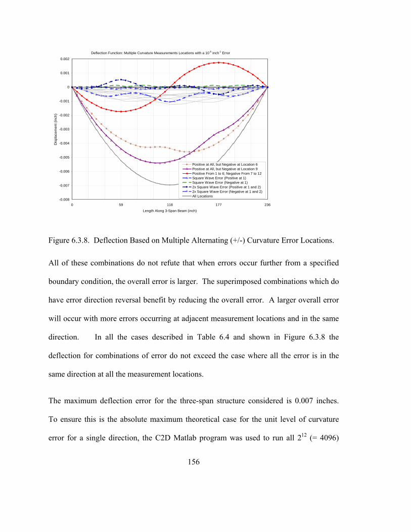
Deflection Function: Multiple Curvature Measurements Locations with a 10-6 inch-1 Error
-0.008
-0.007
-0.006
-0.005
-0.004
-0.003
-0.002
-0.001
0
0.001
0.002
0 59 118 177 236
Length Along 3-Span Beam (inch)
Dis
plac
emen
t (in
ch)
Positive at All, but Negative at Location 6Positive at All, but Negative at Location 9Positive From 1 to 6; Negative From 7 to 12Square Wave Error (Positive at 1)Square Wave Error (Negative at 1)2x Square Wave Error (Positive at 1 and 2)2x Square Wave Error (Negative at 1 and 2)All Locations
Figure 6.3.8. Deflection Based on Multiple Alternating (+/-) Curvature Error Locations.
All of these combinations do not refute that when errors occur further from a specified
boundary condition, the overall error is larger. The superimposed combinations which do
have error direction reversal benefit by reducing the overall error. A larger overall error
will occur with more errors occurring at adjacent measurement locations and in the same
direction. In all the cases described in Table 6.4 and shown in Figure 6.3.8 the
deflection for combinations of error do not exceed the case where all the error is in the
same direction at all the measurement locations.
The maximum deflection error for the three-span structure considered is 0.007 inches.
To ensure this is the absolute maximum theoretical case for the unit level of curvature
error for a single direction, the C2D Matlab program was used to run all 212 (= 4096)
156
binary combinations for the selected beam. The result of the Matlab C2D run is shown in
Figure 6.3.9. Indeed the maximum error determined by the C2D calculation is the same
as that determined by the superposition of the previous individual error data. Considering
error direction reversals, a trinary number of combinations equal to 312 (= 531,441)
would include all possible combinations. The C2D method was initiated; however, the
required computation capacity was not available to complete the analysis. A
supercomputer platform; alternate programming software; or more efficient coding, is
probably better suited to perform this analysis.
0 59 118 177 236-8
-7
-6
-5
-4
-3
-2
-1
0
1
2x 10⁻³
Length of Beam = 236 inches
Def
lect
ion
(in)
All Possible Positive Unit Error Combinations for the Three Span Beam
Figure 6.3.9. All Possible Positive Error Combination Displacement Functions.
In any event, the results of the binary analysis for single direction (Figure 6.3.9) give the
maximum error envelope based on superposition. This result is based on a unit
magnitude of error (10-6 inch-1 of curvature) at a single measurement location. This error
envelope can be used to estimate the expected displacement error of the C2D method.
After determining the expected maximum error of the curvature measurements due to
157

158
noise, and or digitization round off, a confidence envelope could be shown on the
deflection diagram as well. It is more difficult to compensate for error during real-time
dynamic or continuous measurements, so a confidence interval is useful; this will be
demonstrated in section 6.3.2.2.
6.3.2.2 Dynamic or Multiple Measurements
The simplest way to reduce random signal error is to acquire that signal at a static
condition of the tested structure and average many readings. However, in many cases, a
dynamic or continuous signal is the desired data product. Often signal conditioning
equipment is the only practical device that can be used; the errors recorded after signal
conditioning will remain a characteristic of the data collected. When we choose
transducers such as an LVDT to measure displacement, we specify a resolution such that
we can measure the movement we expect to see with reasonable accuracy. The deflected
shape envelope developed in section 6.3.2.1 can be used to help calculate the expected
resolution or noise associated with a specific configuration of curvature measurements
and the C2D method. This section shows an example of this as applied to the same
three-span continuous small scale beam that is described in chapter 5.
The overall process involves first determining the expected signal error and its
characteristics as described in section 6.2.3. The analysis should result in a reasonable
quantity of expected signal error. It could be expressed as the standard deviation of error;
or as the maximum expected error; or the 95th percentile confidence error, or any variety
of statistical quantities. The only qualification is that the signal error should describe an

159
error relative to the mean of the measured phenomenon over a long period of time at a
stable loading condition. Some possible statistical descriptors, and their quantities, are
shown in Table 6.5. The table is generated from data shown in Figure 6.2.11. The table
shows the statistical properties of the 12 Fabry-Perot fiber optic strain gauges used on the
three-span scale model.
The second step is to convert the signal error of the device into its corresponding error in
the curvature measurement. This error is highly dependant on the method of obtaining
the curvature; the constitutive and kinematic relationships will supply the equations that
relate the measured quantity to curvature. If multiple devices are used to measure a
single curvature state, their error will propagate through the equations used. If an
averaging or line fitting technique is employed to obtain curvature from many
measurements, then that process should be used to obtain the overall error of the
curvature measurement. In this section, the example calculation is based on a single
strain reading to obtain the beam curvature.
An alternate technique is to combine the first and second step. Acquire static data over
time from all the devices used and calculate the curvature directly. The calculated
curvature can then be characterized as a signal to obtain its error. Whichever technique is
used, the curvature signal error obtained is used in the next step: it can also be called the
curvature resolution.
The magnitudes of the curvature signal error is simply a scalar multiple of the unit
curvature error (10-6 inch-1) used to analyze the C2D method in previous sections. Those
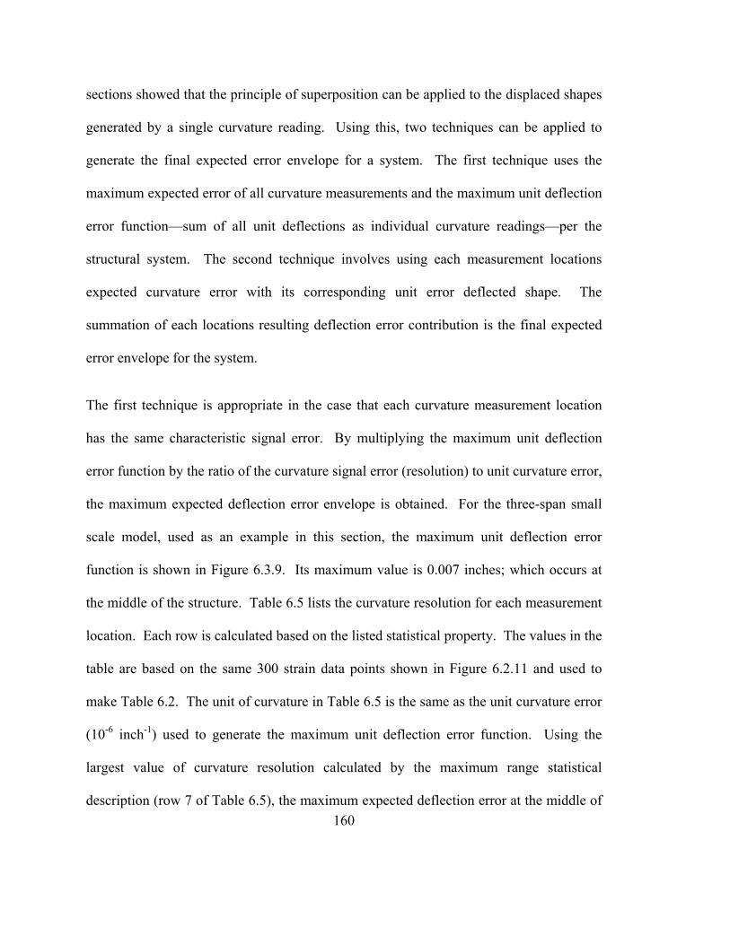
160
sections showed that the principle of superposition can be applied to the displaced shapes
generated by a single curvature reading. Using this, two techniques can be applied to
generate the final expected error envelope for a system. The first technique uses the
maximum expected error of all curvature measurements and the maximum unit deflection
error function—sum of all unit deflections as individual curvature readings—per the
structural system. The second technique involves using each measurement locations
expected curvature error with its corresponding unit error deflected shape. The
summation of each locations resulting deflection error contribution is the final expected
error envelope for the system.
The first technique is appropriate in the case that each curvature measurement location
has the same characteristic signal error. By multiplying the maximum unit deflection
error function by the ratio of the curvature signal error (resolution) to unit curvature error,
the maximum expected deflection error envelope is obtained. For the three-span small
scale model, used as an example in this section, the maximum unit deflection error
function is shown in Figure 6.3.9. Its maximum value is 0.007 inches; which occurs at
the middle of the structure. Table 6.5 lists the curvature resolution for each measurement
location. Each row is calculated based on the listed statistical property. The values in the
table are based on the same 300 strain data points shown in Figure 6.2.11 and used to
make Table 6.2. The unit of curvature in Table 6.5 is the same as the unit curvature error
(10-6 inch-1) used to generate the maximum unit deflection error function. Using the
largest value of curvature resolution calculated by the maximum range statistical
description (row 7 of Table 6.5), the maximum expected deflection error at the middle of

the continuous beam is 8.4436 x (0.007 inches) = 0.0591 inches. The maximum unit
curvature error function is the plotted as the heavy grey line in Figure 6.3.10.
The second technique applies each measurement’s individual error deflection
contribution to establish the total expected deflection error function. By multiplying the
unit deflection error function, per measurement location, by the ratio of the curvature
resolution to unit curvature error, at that location, the result is the expected deflection
error envelope contribution of that curvature measurement. Summing all the resulting
functions from each measurement location throughout the beam, the total expected
deflection error function of the structural system is established. For the example
structure, the curvature resolution is listed in Table 6.5; the unit deflection error functions
are shown in Figure 6.3.6. The total deflection error function that results from using the
maximum range curvature resolution descriptor (row 7 of Table 6.5) is shown in Figure
6.3.10. The unit deflection error functions for each curvature measurement are plotted in
light gray. The total deflection error function has a smaller magnitude of error than the
maximum expected error function as shown in the figure.
Table 6.5. Small Scale Three Span Beam Signal Error Characteristics Summary.
161
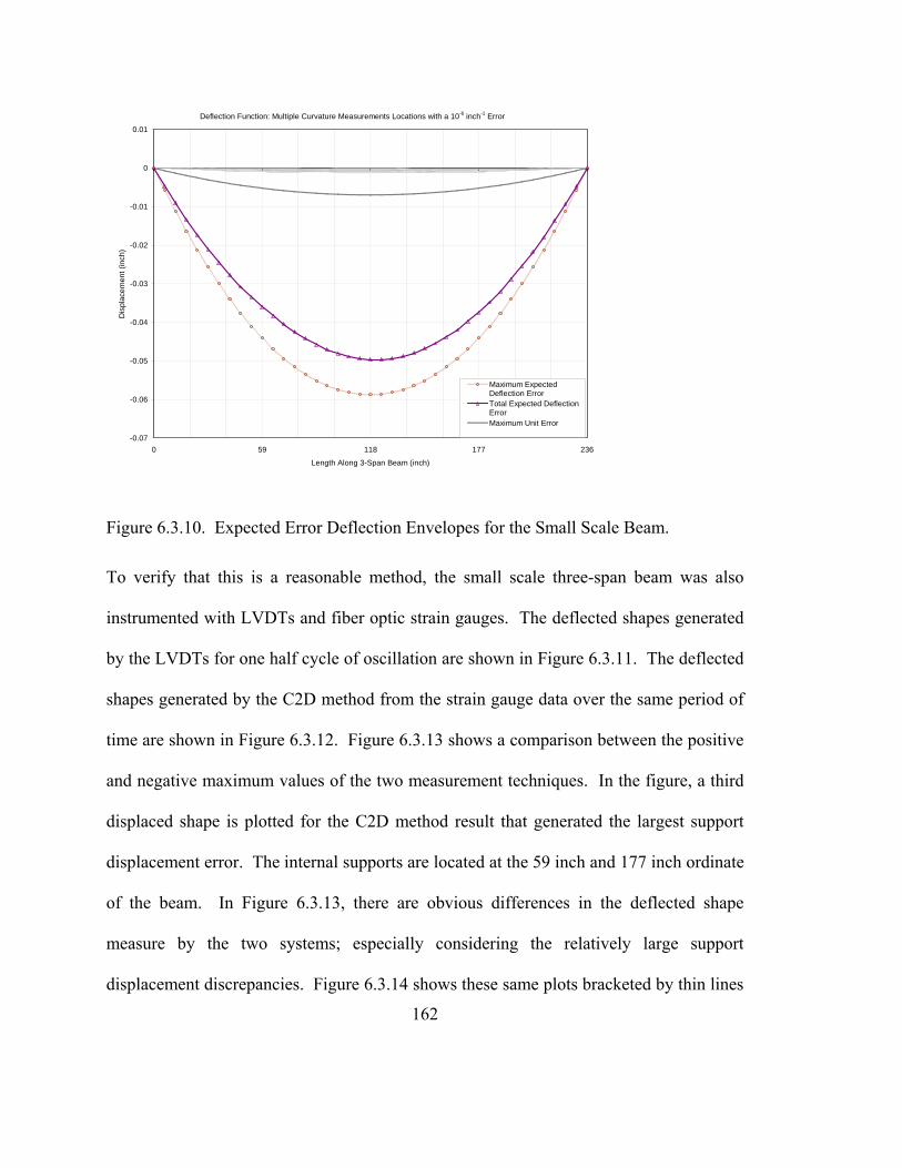
Deflection Function: Multiple Curvature Measurements Locations with a 10-6 inch-1 Error
-0.07
-0.06
-0.05
-0.04
-0.03
-0.02
-0.01
0
0.01
0 59 118 177 236
Length Along 3-Span Beam (inch)
Dis
plac
emen
t (in
ch)
Maximum ExpectedDeflection ErrorTotal Expected DeflectionErrorMaximum Unit Error
Figure 6.3.10. Expected Error Deflection Envelopes for the Small Scale Beam.
To verify that this is a reasonable method, the small scale three-span beam was also
instrumented with LVDTs and fiber optic strain gauges. The deflected shapes generated
by the LVDTs for one half cycle of oscillation are shown in Figure 6.3.11. The deflected
shapes generated by the C2D method from the strain gauge data over the same period of
time are shown in Figure 6.3.12. Figure 6.3.13 shows a comparison between the positive
and negative maximum values of the two measurement techniques. In the figure, a third
displaced shape is plotted for the C2D method result that generated the largest support
displacement error. The internal supports are located at the 59 inch and 177 inch ordinate
of the beam. In Figure 6.3.13, there are obvious differences in the deflected shape
measure by the two systems; especially considering the relatively large support
displacement discrepancies. Figure 6.3.14 shows these same plots bracketed by thin lines
162

163
that represent the total expected deflection error due to the signal noise characteristics of
the fiber optic strain gauges used. While the error envelopes look too large to be useful,
they do show that the LVDT displaced shapes fall within the estimated maximum error.
The zero displacement at the interior supports also falls within the range of error for that
C2D result as well. Figure 6.3.15 shows a time history of the deflection at the midpoint
of the middle span of the structure. In the figure, the total expected deflection error is
rarely reached. In the figure, the LVDT deflection is considered the true deflection so the
error deflection limits are offset from that reference point. This figure shows that
different statistical descriptors of the signal error will reasonably represent a majority of
the data collected over a period of time. It is up to the user to choose an acceptable
confidence interval. This process can be repeated on any C2D instrumentation scheme to
help identify the resulting resolution of deflection.
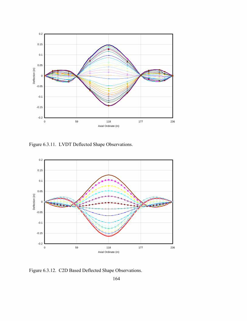
-0.2
-0.15
-0.1
-0.05
0
0.05
0.1
0.15
0.2
0 59 118 177 236
Axial Ordinate (in)
Def
lect
ion
(in)
Figure 6.3.11. LVDT Deflected Shape Observations.
-0.2
-0.15
-0.1
-0.05
0
0.05
0.1
0.15
0.2
0 59 118 177 236
Axial Ordinate (in)
Def
lect
ion
(in)
Figure 6.3.12. C2D Based Deflected Shape Observations.
164

-0.2
-0.15
-0.1
-0.05
0
0.05
0.1
0.15
0.2
0 59 118 177 236
Axial Ordinate (in)
Def
lect
ion
(in)
C2D Upward
C2D Support Error
C2D Downward
LVDT Upward
LVDT Downward
Figure 6.3.13. LVDT & C2D Maximum Measured Displacements.
-0.2
-0.15
-0.1
-0.05
0
0.05
0.1
0.15
0.2
0 59 118 177 236
C2D Upward C2D Downward LVDT UpwardLVDT Downward
-0.2
-0.15
-0.1
-0.05
0
0.05
0.1
0.15
0.2
0 59 118 177 236
C2D Support Error
Figure 6.3.14. C2D Error Envelope Comparison with LVDT and Support Measurements.
165

Mid-Span Displacement versus Time
-0.06
-0.04
-0.02
0
0.02
0.04
0.06
4.5 4.6 4.7 4.8 4.9 5 5.1 5.2 5.3 5.4 5.5
Time (seconds)
Dis
plac
emen
t (in
ches
)
LVDT Deflection
C2D Calculated Deflection
C2D Total Error Deflection Limits
C2D Std. Dev. Of Error Deflection Limits
C2D 2x Std. Dev. Of Error Deflection Limits
Figure 6.3.15. Comparison of Error Envelopes for Deflection at Location of an LVDT.
6.4 Comments on Error Reduction Methods for C2D Method
The errors noted in the previous sections can be mitigated to some extent by various
methods. This section will highlight some possible ways to reduce the error that exists
for the C2D method of determining beam deflection. Some methods discussed here
include: post processing data averaging and adaptations to the C2D method
discretization.
6.4.1 Post Processing Data Averaging
There are a lot of signal analysis techniques that can be utilized during a post processing
regime. In structural testing, most of the useful data has been analyzed with post
processing. A large hurdle to overcome in real-time structural health monitoring is to
166

167
perform all the calculations that convert the raw signal data into useful, structurally
significant, quantities for real-time decision making. At this time, for the typical
application, the C2D methodology is itself not likely usable for a true real-time structural
health monitoring application; it is more appropriately used with a post-processing
routine. Data averaging can easily be incorporated to improve the observations by the
C2D method. A few data averaging techniques are applied for static measurements and
for dynamic measurements in this section. The impact on the acquired data is discussed
by use of selected examples.
6.4.1.1 Static Measurements
Data averaging can help to improve the analysis of a beam’s deflection when there is a
difference between the assumed boundary conditions and the real boundary conditions of
the structure. In the case of the three-span small scale beam defined in chapter 5, the
actual boundary conditions of the real structure effect the assumptions used to measure
curvature as a result of axial loading that may or may not be considered in the idealized
structure.
By averaging two or more strain readings at a particular curvature measurement location,
the axial strain can be indicated. This may not directly eliminate error in the deflected
shape; however, it may help to provide a clue as to other effects that may be causing
strange results for the deflected shape. If only a single strain gauge were used to acquire
data for the C2D method input, the axial strain will cause significant errors.

In another case, directly averaging curvature measurements, over time, eliminates noise
from the individually obtained deflection results. For example, data was collected from
the three-span small scale beam setup at a frequency of 100 Hz for 2.5 seconds at four
different static loading conditions. Figure 6.4.1 shows the deflection calculated by the
C2D method. The plot on the left is of the raw data—250 deflection curves for each load
condition. The plot on the right results from averaging all 250 raw data points for each
load condition. The averaged data clearly show the difference between the four load
conditions; there is no guarantee that a single raw data point would reproduce such a
clear representation.
0 59 118 177 236-0.08
-0.07
-0.06
-0.05
-0.04
-0.03
-0.02
-0.01
0
0.01
0.02
Def
lect
ion
of B
eam
(in)
Plot of Deflection for the Three Span Beam
0 59 118 177 236-0.08
-0.07
-0.06
-0.05
-0.04
-0.03
-0.02
-0.01
0
0.01
0.02
Def
lect
ion
of B
eam
(in)
Plot of Deflection for the Three Span Beam
Figure 6.4.1. Before (Left) and After (Right) Averaging C2D Static Displacements.
6.4.1.2 Dynamic Measurements
During dynamic measurements, the luxury of averaging many data sets is not always
possible. Depending on the structural system and measurement capabilities of the data
168
169
acquisition system, an optimum number of data points averaged can be determined.
Sometimes, the averaging solution may include using a weighted averaging technique.
The simplest averaging technique for dynamic data is the use of a rectangular averaging
window. The rectangular averaging window is defined such that an equal weight is
applied to each of the data points used to calculate the final value. The averaging
windows length is specified in terms of number of data points. Two triangular weighting
functions are also tested.
6.4.1.2.1 Determined At a Single Location with an LVDT
An example of using the rectangular averaging windows with the C2D method is shown
here for the deflection calculated at the location of a single LVDT measurement at the
mid-span of a beam. To see the effect of different lengths of the averaging window, the
deflection versus time was plotted for three cases. Four deflection data sets are compared
in Figure 6.4.2: LVDT measurements; C2D calculated deflection based on raw data; C2D
calculated deflection based on a rectangular window with four data points averaged; C2D
calculated deflection based on a rectangular window with eight data points averaged.

-0.04
-0.03
-0.02
-0.01
0
0.01
0.02
0.03
0.04
4.5 4.6 4.7 4.8 4.9 5 5.1 5.2 5.3 5.4 5.5
Time (seconds)
Def
lect
ion
(inch
)
LVDT01(in)raw (in)ave 4 (in)ave 8 (in)
Figure 6.4.2. Rectangular Averaging Windows Effects on Deflection.
The LVDT plot provides a clean displacement signal; it will provide a consistent modal
frequency and damping ratio calculation. Notice that the raw data does follow the LVDT
deflection; however, it has a larger amount of noise and probably will not produce a
consistent modal frequency or damping ratio. The C2D plot that is generated by an
averaging window with a length of four data points follows the LVDT data more tightly
than the noisy raw signal. It can be seen that the modal frequency and damping ratio can
probably be extracted more consistently than from the raw data plot as well. The C2D
plot that is generated by an averaging window with a length of eight data points is a
smoother signal; however, the displacement peaks during the free vibration are clipped.
The modal frequency can probably still be calculated, however, the clipping of the
displacements will likely not produce the correct damping ratio.
170

171
To try to mitigate the clipping effect observed in the eight point rectangular averaging
window case, triangular averaging windows were tried using the same four and eight data
point lengths. For the four data point case, the weights applied from oldest to newest data
point were 0.1, 0.2, 0.3, and 0.4. For the eight data point case, the weights applied from
oldest to newest data point were 1/36, 2/36, 3/36, 4/36, 5/36, 6/36, 7/36, and 8/36. Figure
6.4.3, shows an improvement in the peak magnitude when using the eight point triangular
averaging windows. There was no significant difference for the four point data averaging
whether rectangular or triangular windows were used. The improvement for the eight
point case might help to identify the damping ratio, however, in the figure this is likely
only the case for the positive displacements during the free vibration. There is likely a
best window length and weighting function to preserve as many structural properties as
possible.
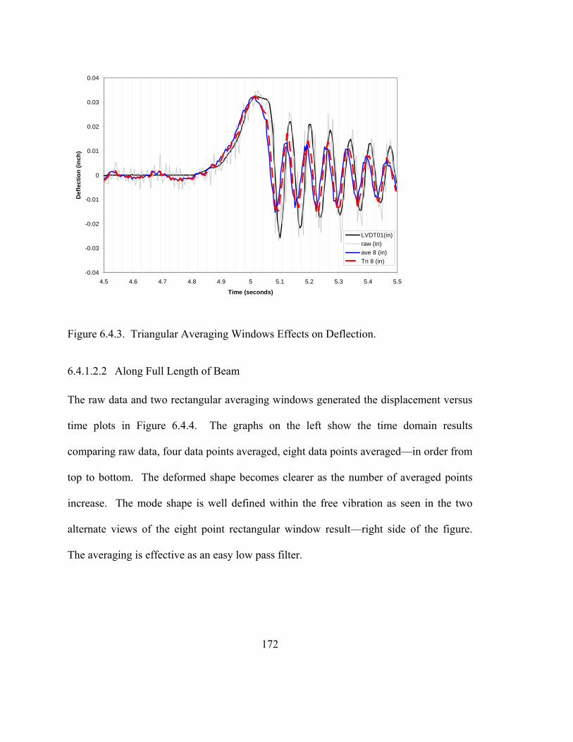
-0.04
-0.03
-0.02
-0.01
0
0.01
0.02
0.03
0.04
4.5 4.6 4.7 4.8 4.9 5 5.1 5.2 5.3 5.4 5.5
Time (seconds)
Def
lect
ion
(inch
)
LVDT01(in)raw (in)ave 8 (in)Tri 8 (in)
Figure 6.4.3. Triangular Averaging Windows Effects on Deflection.
6.4.1.2.2 Along Full Length of Beam
The raw data and two rectangular averaging windows generated the displacement versus
time plots in Figure 6.4.4. The graphs on the left show the time domain results
comparing raw data, four data points averaged, eight data points averaged—in order from
top to bottom. The deformed shape becomes clearer as the number of averaged points
increase. The mode shape is well defined within the free vibration as seen in the two
alternate views of the eight point rectangular window result—right side of the figure.
The averaging is effective as an easy low pass filter.
172

Figure 6.4.4. Comparison of Rectangular Averaging Windows for the Entire Beam.
6.4.2 C2D Method Adaptations
The following subsections highlight other techniques that can be applied as well. These
adaptations have not yet been tried by the author, however, the error-inducing behavior
observed during the sensitivity analysis preceding this section suggest that they may
provide improvements to the system.
173

174
6.4.2.1 Number of Beam Sections
By changing the number of beam sections, there are more data points that are acquired
that will help to match the curvature function. The problem associated with point loads
applied within beam sections will be reduced in two ways. First, there will be more
locations where the point load may occur such that it satisfies the exact solution—
application at the ends of beam sections. Second, even if the point load falls within a
beam section, the mismatched curvature diagram is only affected within that beam
section. As the error propagates through the double integration, the error is applied to a
shorter length of beam. The overall error will be reduced.
6.4.2.2 Alternate Curvature Estimate Implementations
The method shown in chapter 5 fits a second degree polynomial to three curvature
readings. This implementation provides the exact solution for a beam element loaded
with either a uniformly distributed load along the entire length of the beam element or
discrete loads applied at the end of each beam element. When this is the case, and the
error is small, the system works very well. Utilizing other functions that represent
different loading conditions for beam elements will likely produce beneficial results.
6.4.2.3 Multiple Implementation Comparison
Another way to help identify loading conditions, and the proper displaced shapes, is to
run several parallel alternate solutions and compare the results. For example, for the real
data cases tested earlier in this chapter, it was common that the curvature diagram was
not continuous. This is obviously possible since the solution described is a C1 continuous

175
solution for displacement; however, in many cases, especially within the long span of a
bridge structure, moments might not be applied between beam sections. The curvature
diagram, or M/EI diagram, is C0 continuous in this case. So it may be useful to compare
a solution that requires inter-sectional curvature continuity—this can be done with a third
degree polynomial curvature function assumption applied incrementally across all the
beam sections.
6.5 Conclusions
The purpose of this chapter was to analyze how errors in indicated strain, or curvature
measurements, affect the results of the C2D methodology for calculating the deflection of
beams. Understanding the implications of the discussed topic toward a particular
structural health monitoring program should help to better plan an instrumentation
strategy. Modifications to the strategy can include transducer placement, transducer type,
curvature estimate formulation, and data smoothing techniques. Currently we see, the
signal noise and significant digits of measurement ultimately control the accuracy of the
C2D methodology. As curvature measurements become more accurate and more stable,
the method will perform better.
Greater accuracy in curvature measurement will help to minimize error in two ways.
First, if accuracy of curvature is carried to enough significant digits for all measurements,
the deviation of the estimated curvature function along the length will be reduced. This
in turn will minimize the cumulative error induced through the integrated angle of
rotation and subsequent displacement functions.

176
Second, loads within a beam element which do not conform to the exact solution that is
best represented by a second degree polynomial curvature function will only generate
significant error in the deflected shape within that element. All other elements that exist
within that structure will provide a reasonably accurate deflected shape assuming
sufficient accuracy of strain / curvature measurements.
Some possible strategies to reducing error through other alternate strategies are suggested
for further study in section 6.4.2. Some of which include changing the number of beam
sections, using a different function to estimate curvature in the beam section, and
providing an algorithm that compares the results of several implementation strategies.

177
CHAPTER 7. SHM DURING HANAPEPE RIVER BRIDGE LOAD TESTING
7.1 Background
The Hanapepe Bridge is located in Hanapepe, Hawaii on the west side of the island of
Kauai. The bridge runs east-west across the Hanapepe River as part of Highway 50
(Kaumaualii Highway) between Waimea and Lihue. According to a previous inspection
report performed by a consulting firm in 2001, the bridge is structurally deficient. While
it may be rehabilitated, there is some question as to whether it should be replaced. To
address concerns regarding this bridge, a load test was requested of Nagamine Okawa
Engineers Inc. The instrumentation described here was designed to measure several
indicators of structural health; static load-deflection behavior, dynamic traffic load
deflection behavior, and loaded shear and flexural crack opening behavior. The
instrumentation used include: LVDT-taut-wire baseline systems, LVDTs, crack gauges,
and pin-support rotation monitoring devices. The intent of the structural health
monitoring system is to provide additional information, beyond visual inspection, for
engineers to validate/calibrate a computer model of the bridge to properly determine the
present capacity of the bridge. Ultimately, the data is used to obtain a field calibrated
analytical model that will be used to justify a recommendation on the status of the
bridge—answering the question, “Is the bridge structurally deficient?”
7.2 Bridge SHM Instrumentation
The instrumentation was installed on one girder of the bridge—Girder G-3. This girder
was selected because it was deemed to be the most deteriorated girder (of four) on the

178
bridge—by visual inspection. To save on cost most of the gauges were installed on the
Lihue half of the bridge—the symmetry of the statically determinate structure helped in
the decision as well. A selection of the largest existing cracks, which existed throughout
the entire length of the beam, were instrumented with gauges.
All LVDTs, crack gauges and rotation sensors were monitored by a National Instruments
data acquisition system running LabVIEW™ software. The data acquisition system was
set to monitor each sensor at a frequency of 25 hertz during each static and dynamic
loading condition. For the static load conditions, 25 successive readings were averaged
for each sensor to minimize potential effects of gauge sensitivity to wind and other
effects. Sensor calibration was adjusted for the electronic lead length required to connect
each sensor to the data acquisition system (see sections 2.2.3 and 2.2.4 for process and
calibration details). The data acquisition system was housed in a minivan located near
the Lihue abutment (Figure 7.2.1). Near real-time deflection and crack gauge plots were
prepared after each load condition to ensure no unexpected response had occurred.

Figure 7.2.1. Data Acquisition System.
A total of 19 electronic gauges were used to acquire data. Two LVDT-taut-wire baseline
systems equipped with a total of six LVDTs were used to measure vertical deflection of
the Lihue abutment span and the center span. An optical survey of the roadway surface
was performed before all testing, during the heaviest loading patterns, and after static
testing for comparison with the LVDT-taut-wire baseline systems. One LVDT was used
to measure the horizontal displacement in the longitudinal direction at the Lihue
abutment. Ten crack gauges were used to monitor crack mouth opening displacements
on selected cracks during the load test. Two Wheatstone bridge based deflection gauges
were used to monitor the rotation at the Lihue pier. These were used to verify/augment
the two LVDT-taut-wire baseline systems—to ensure continuity of deflection
measurements across the Lihue Pier.
179

The automated data acquisition system was powered by a Honda EU1000i generator—
this generator is equipped with a low noise regulated true sine wave inverter and designed
for use with sensitive computer equipment. A true sine wave backup power supply was
also used to ensure no power loss to the data acquisition system in case the generator
needed to be refueled.
7.2.1 Vertical Deflection
Vertical deflections of the Lihue abutment span and the center span were monitored by
two LVDT-taut-wire baseline deflection monitoring systems. Chapter 3 has a full
discussion on the design of such a system. The baseline system consists of a high-
strength piano wire spanning the full length of the span to be monitored, and tensioned by
means of a tensioning weight hanging over a pulley at the live end of the baseline system.
Figure 7.2.2 shows a schematic of this system in both the center span and the Lihue
abutment span. Figure 7.2.3, Figure 7.2.4, and Figure 7.2.5 show more details of the
systems in each span.
Figure 7.2.2. Elevation of Girder G-3 Showing LVDT-Taut-Wire Baseline Systems.
180
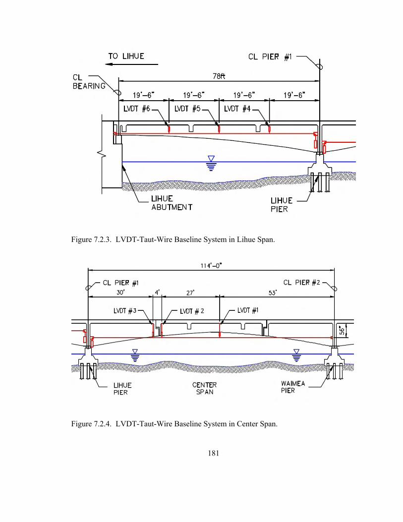
Figure 7.2.3. LVDT-Taut-Wire Baseline System in Lihue Span.
Figure 7.2.4. LVDT-Taut-Wire Baseline System in Center Span.
181
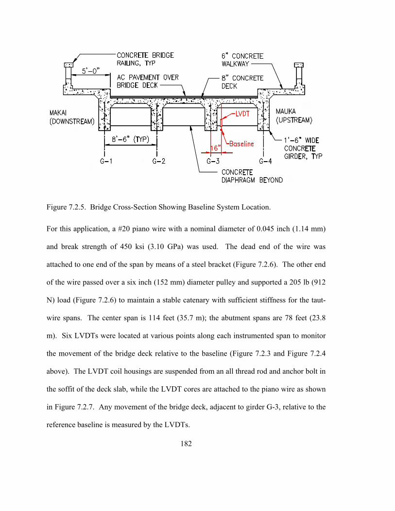
Figure 7.2.5. Bridge Cross-Section Showing Baseline System Location.
For this application, a #20 piano wire with a nominal diameter of 0.045 inch (1.14 mm)
and break strength of 450 ksi (3.10 GPa) was used. The dead end of the wire was
attached to one end of the span by means of a steel bracket (Figure 7.2.6). The other end
of the wire passed over a six inch (152 mm) diameter pulley and supported a 205 lb (912
N) load (Figure 7.2.6) to maintain a stable catenary with sufficient stiffness for the taut-
wire spans. The center span is 114 feet (35.7 m); the abutment spans are 78 feet (23.8
m). Six LVDTs were located at various points along each instrumented span to monitor
the movement of the bridge deck relative to the baseline (Figure 7.2.3 and Figure 7.2.4
above). The LVDT coil housings are suspended from an all thread rod and anchor bolt in
the soffit of the deck slab, while the LVDT cores are attached to the piano wire as shown
in Figure 7.2.7. Any movement of the bridge deck, adjacent to girder G-3, relative to the
reference baseline is measured by the LVDTs.
182

Figure 7.2.6. Taut-Wire Baseline Dead (Left) and Live (Right) End Supports.
Figure 7.2.7. LVDT-Taut-Wire Baseline LVDT Support Details.
183
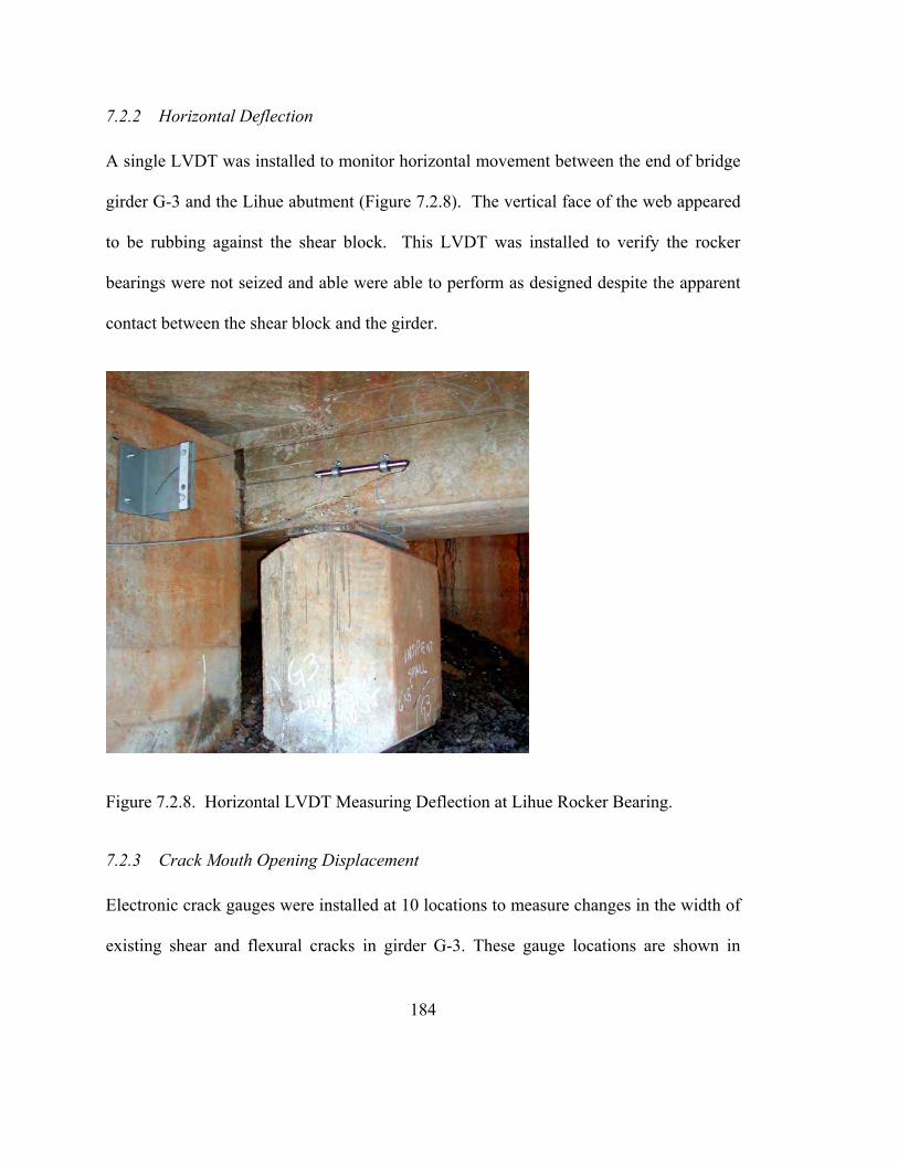
7.2.2 Horizontal Deflection
A single LVDT was installed to monitor horizontal movement between the end of bridge
girder G-3 and the Lihue abutment (Figure 7.2.8). The vertical face of the web appeared
to be rubbing against the shear block. This LVDT was installed to verify the rocker
bearings were not seized and able were able to perform as designed despite the apparent
contact between the shear block and the girder.
Figure 7.2.8. Horizontal LVDT Measuring Deflection at Lihue Rocker Bearing.
7.2.3 Crack Mouth Opening Displacement
Electronic crack gauges were installed at 10 locations to measure changes in the width of
existing shear and flexural cracks in girder G-3. These gauge locations are shown in
184

Figure 7.2.9 through Figure 7.2.12. A number of these gauges were located close to
previously installed long-term optical crack monitor stations, see Figure 7.2.13.
Crack gauges 1, 2, 6, and 7 are located on shear cracks in the cantilever girders
supporting either end of the drop-in section of the center span. Crack gauge 3 is located
on a shear crack in the drop-in section. Crack gauges 4 and 5 are located over flexural
cracks at midspan of the center span drop-in section. Crack gauges 8 and 9 are on shear
cracks in the Lihue abutment span. Crack gauge 10 is on the soffit of girder G-3 over a
flexural crack in the Lihue span.
Figure 7.2.9. Crack Gauge on Downstream Elevation of Center Span.
185

Figure 7.2.10. Crack Gauges on Downstream Elevation of Lihue Span.
Figure 7.2.11. Crack Gauges on Upstream Elevation of Center Span.
186

Figure 7.2.12. Crack Gauges on Upstream Elevation of Lihue Span.
Figure 7.2.13 and Figure 7.2.14 show the typical installation of the electronic crack
gauges. The crack gauges were fabricated specifically for this project. Each gauge
consisted of a C-shaped aluminum plate instrumented with electrical resistance strain
gauges and calibrated to accurately measure changes in the gauge opening (See Chapter 4
for design details). Mounting tabs were epoxied to either side of the crack to be
monitored, and the crack gauge installed as shown in Figure 7.2.14. Notice the strain
relief screw and washer used to eliminate the influence of cable movement. The
aluminum tabs were spaced at 0.125 inches (3.18 mm) by using a machined spacer bar—
this also insured that they were installed parallel. The gauges clip onto the tabs such that
187

they will measure the crack closing as well as opening—they maintain their contact with
the aluminum tabs for any crack mouth opening displacement. The grooves milled into
the outside ends of the tabs are cut to align and hold secure the sharpened edge of the clip
gauge—ensuring a true pin support at the gauge to aluminum tab interface.
Figure 7.2.13. Crack Gauge 9 Adjacent to Visual Crack Monitor 3.
188

Figure 7.2.14. Typical Crack Gauge (10) on Mounting Tabs.
Table 7.1 gives details related to each crack gauge, including location, crack type,
adjacent crack monitor number, and original estimated crack width (based on prior visual
inspection). Reference Figure A7.2.17 through Figure A7.2.25 in the Appendix—photos
of all the installed crack gauges.
189

Table 7.1. Crack Gauge Details.
7.2.4 Rotation at Lihue Pier Support
Two custom-designed high-resolution displacement sensors were fabricated to monitor
the rotation of girder G-3 over the Lihue pier. See chapter 4 for design details. The
sensors were attached to steel brackets on either side of the bearing as shown in Figure
7.2.15 and Figure 7.2.16. The measured rotation was used to confirm the slope of the
deflected shape as measured by the baseline systems on either side of the Lihue pier.
190
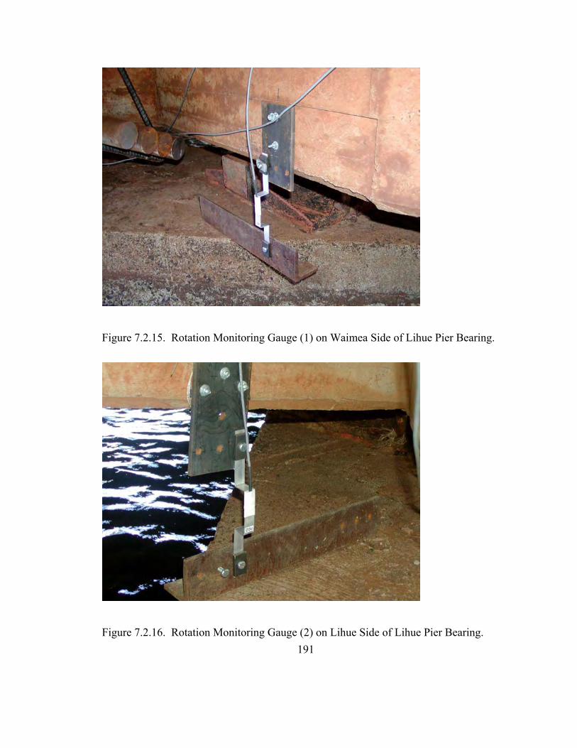
Figure 7.2.15. Rotation Monitoring Gauge (1) on Waimea Side of Lihue Pier Bearing.
Figure 7.2.16. Rotation Monitoring Gauge (2) on Lihue Side of Lihue Pier Bearing. 191

7.3 Data Acquisition and Processing
7.3.1 Optical Survey
In order to verify the two LVDT-Taut-Wire baseline deflection systems, optical surveys
of the bridge roadway were performed during each of the heaviest loading conditions.
The heaviest load series was anticipated to have deflections of an order that could be
measured by optical survey. The smallest recordable increment of displacement for the
theodolite and rod used is 0.06 inches (1.52 mm). The survey points are shown in Figure
7.3.1. Survey points G1 through G6 are located over girder G-3, at the same locations as
LVDTs 1 to 6 on the baseline systems. Survey points C1 through C6 are located on the
centerline of the roadway corresponding to G1 through G6, but adjusting for the 45°
bridge skew. Survey points GS and CS are located over the Lihue Pier to measure any
settlement of the pier during the load test.
Figure 7.3.1. Optical Survey Points.
192

193
7.3.2 Temperature Effects
The load test started at about 12:00 AM and ended at 3:30 AM. During this time, the
bridge roadway was cooling down, affecting the deflected shape of the bridge. The final
deflected shape after removal of the truck loads differed from the initial deflected shape
as shown in Figure 7.3.2. Although no thermal measurements or thermal analysis was
performed on the bridge, the likely thermal effects can be inferred from the H3 North
Halawa Valley Viaduct records. Numerous thermocouples were embedded in the NHVV
during construction, and monitored for 10 years (Figure 7.3.3 and Figure 7.3.4). A typical
daily temperature variation at the top of the roadway (sensor 14) and lower in the cross-
section (sensor 21) shows that the thermal changes are limited to the top surface of the
superstructure.
During the 12:00 AM to 3:30 AM time period, the thermal variation at all sensors in the
NHVV was approximately linear (Figure 7.3.3). Linear interpolation was therefore used
to adjust the Hanapepe Bridge load test results based on the difference between the
original deflected shape and the final deflected shape.
Figure 7.3.2 shows the thermal adjustment based on initial and final zero deflection
measurements. The initial deflection measurements are all set to zero before any truck
load was applied to the bridge. These readings were taken at 12:00 AM. The final
readings taken after all truck load tests had been performed, shows that the bridge
deflection has changed during the load test due to cooling of the roadway surface, as
previously observed on the H3 NHVV. As the top surface cools, the bridge forms a
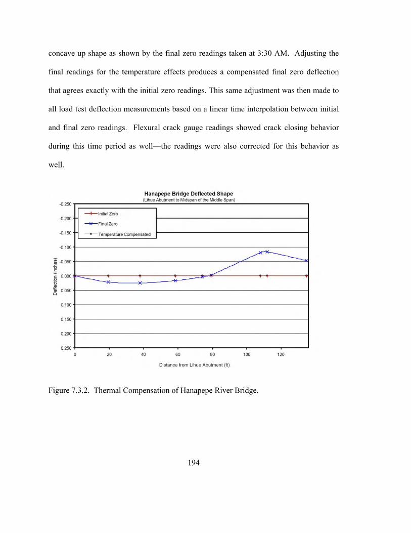
concave up shape as shown by the final zero readings taken at 3:30 AM. Adjusting the
final readings for the temperature effects produces a compensated final zero deflection
that agrees exactly with the initial zero readings. This same adjustment was then made to
all load test deflection measurements based on a linear time interpolation between initial
and final zero readings. Flexural crack gauge readings showed crack closing behavior
during this time period as well—the readings were also corrected for this behavior as
well.
Figure 7.3.2. Thermal Compensation of Hanapepe River Bridge.
194

Figure 7.3.3. Thermocouple Locations on H3 North Halawa Valley Viaduct [Robertson
& Ingham 1999].
Figure 7.3.4. H3 North Halawa Valley Viaduct Daily Temperature Variation [Robertson
& Ingham 1999].
195

196
7.4 Load Test Program
The purpose of the load test was to determine the load ratings of the bridge and evaluate
its short term performance in terms of service loads. This test program is not a proof load
test. The load rating is instead evaluated through observing the elastic behavior of the
bridge to assist in calibrating a computer model.
The load used includes different configurations of three trucks of varying weight as
described in section 7.4.1. The bridge is on the main thoroughfare connecting Lihue and
Waimea—the only route for heavy truck traffic. During the nighttime testing, all light
vehicle traffic was diverted; any heavy traffic was allowed to pass.
7.4.1 Truck Loads
All truck axle loads were measured using a calibrated load scale prior to testing. Each of
the three truck’s dimensions and axle loads are shown in Figure 7.4.1. Truck 1 is the
HDOT’s “reach-all” truck (2003 Aspen Ariels Model UB60). Truck 2 is an HDOT boom
truck while Truck 3 is a rented boom-truck.

Figure 7.4.1. Trucks Loads and Dimensions.
197

198
7.4.2 Static Loading
The static load test involved 6 load series as described in Table 7.2. For each load series,
a selected truck pattern was applied at pre-determined locations on the bridge. Four pre-
determined loading locations were designated as L1 through L4. L1 was at the critical
loading location on the Lihue abutment span, located 30 feet from the Lihue abutment
support bearing. L2 was at the pinned joint in the center span. L3 was such that the rear
wheels of truck 1 were centered over the pinned joint. L4 was at the midspan on the
center span. All load series used loading locations L1, L2 and L4. Loading location L3
was only used for the heaviest load series, LS6.
The results for a particular truck loading condition are referred to using both the load
series and load location. For example, during load series LS6, when the truck load was
centered over midspan of the center span (load location 4), the test is referred to as LS6-
L4. Figure 7.4.2 shows the truck loads in place for LS6-L3 during the load test.
Graphical representations of all truck load conditions are given in the Appendix—Figure
A7.4.3 through Figure A7.4.21. After completing all static loading cases, the trucks were
removed from the bridge to record the final unloaded condition.

Table 7.2. Truck Load Series.
Figure 7.4.2. Truck Load During Load Series 6, Location 3 (LS6-L3).
199

200
7.4.3 Dynamic Loading
A series of four dynamic tests was then performed using only Truck 1. The first two tests
involved driving Truck 1 across the bridge along the centerline of the roadway at 25 mph
in each direction. The first pass was traveling towards Lihue (D1) while the second was
traveling towards Waimea (D2). The third and fourth dynamic tests were the same as D1
and D2 except that the truck brakes were applied as the truck front wheels passed over
the Lihue Pier. Dynamic test D3 was the braking test with the truck traveling towards
Lihue, while D4 was the braking test with the truck traveling towards Waimea. These
dynamic tests were performed to study the impact effect of a truck traveling at speed, and
to monitor any horizontal movement of the bridge during heavy braking.
7.5 Load Test Results
The data acquired during 19 static load cases and 4 dynamic load cases helps us to
understand the current performance of the Hanapepe River Bridge. Please note that all
static load cases were adjusted for the structural deflection due to thermal cooling during
the test period.
7.5.1 Vertical Deflections
7.5.1.1 Load Series 1
Figure 7.5.1 shows the deflected shapes recorded by the LVDT-Taut-Wire baseline
systems during the three load conditions (L1, L2 and L4) of Load Series 1. Recall that
Load Series 1 consisted of Trucks 2 and 3 side-by-side on the bridge roadway (Table

201
7.2). Note that these deflected shapes have all been adjusted for thermal effects as
described in Section 7.3.2.
Under LS1-L1, when the truck load is at the critical section on the abutment span, the
abutment span deflects downwards, as expected, while the hinge in the center span
deflects upwards. The drop-in section of the center span is unloaded, and therefore
remains a straight line segment between the two pinned end conditions. The pinned
condition at the hinge is clearly evident from the kink in the deflected shape.
Under LS1-L2, when the truck load is located over the hinge in the center span, the hinge
deflects downwards, while the abutment span deflects upwards, as would be expected.
The drop-in section at the middle of the center span remains unloaded, and is therefore
still a straight line between the pinned ends.
Finally, under LS1-L4, when the truck load is located at mid-span of the center span, the
hinge deflection remains approximately the same as for LS1-L2, while the abutment span
deflection decreases slightly. The drop-in section at the middle of the center span now
shows a deflected shape similar to a simply supported beam, as would be expected.

Hanapepe Bridge Deflected Shape(Lihue Abutment to Midspan of the Middle Span)
-0.250
-0.200
-0.150
-0.100
-0.050
0.000
0.050
0.100
0.150
0.200
0.2500 20 40 60 80 100 120
Distance from Lihue Abutment (ft)
Def
lect
ion
(inch
es)
LS1-L1LS1-L2LS1-L4
Lihue Pier
Center Span Hinge
L1 L2 L4
Figure 7.5.1. Load Series 1 Deflected Shape of Lihue Half of Bridge.
7.5.1.2 Load Series 2 and 3
Figure 7.5.2 shows the deflected shapes recorded by the baseline systems during each
load condition (L1, L2 and L4) of Load Series 2 and 3. Load Series 2 consisted of Trucks
1 and 2 side-by-side on the bridge roadway with Truck 1 (the larger load) in the upstream
lane (Table 7.2). In Load Series 3, the trucks are reversed so the heavier truck is in the
downstream lane. All deflected shapes are similar to those observed for Load Series 1,
but the measured deflections are slightly larger since the combined truck load is greater
for Load Series 2 and 3.
202

The LVDT-Taut-Wire baseline system records slightly larger deflections under Load
Series 2 than for Load Series 3 because the larger truck load (Truck 1) is more directly
over Girder G-3 and the baseline system for Load Series 2.
Hanapepe Bridge Deflected Shape(Lihue Abutment to Midspan of the Middle Span)
-0.250
-0.200
-0.150
-0.100
-0.050
0.000
0.050
0.100
0.150
0.200
0.2500 20 40 60 80 100 120
Distance from Lihue Abutment (ft)
Def
lect
ion
(inch
es)
LS2-L1LS2-L2LS2-L4LS3-L1LS3-L2LS3-L4
L1 L2 L4
Lihue Pier
Center Span Hinge
Figure 7.5.2. Load Series 2 and 3 Deflected Shape of Lihue Half of Bridge.
7.5.1.3 Load Series 4 and 5
Figure 7.5.3 shows the deflected shapes recorded by the LVDT-Taut-Wire baseline
systems during each load condition (L1, L2 and L4) of Load Series 4 and 5. Load Series
4 consisted of Truck 1 (the largest truck load) in the upstream lane (Table 7.2). In Load
Series 5, Truck 1 is in the downstream lane. All deflected shapes are similar to those
observed for Load Series 1. The total weight of Truck 1 is slightly less than the combined
weight of Trucks 2 and 3 used in Load Series 1. However, when Truck 1 is located over
203

girder G-3 and the baseline system, the deflections measured by the baseline system
increase, as would be expected.
Hanapepe Bridge Deflected Shape(Lihue Abutment to Midspan of the Middle Span)
-0.250
-0.200
-0.150
-0.100
-0.050
0.000
0.050
0.100
0.150
0.200
0.2500 20 40 60 80 100 120
Distance from Lihue Abutment (ft)
Def
lect
ion
(inch
es)
LS4-L1LS4-L2LS4-L4LS5-L1LS5-L2LS5-L4
Lihue Pier
Center Span Hinge
L1 L2 L4
Figure 7.5.3. Load Series 4 and 5 Deflected Shape of Lihue Half of Bridge.
7.5.1.4 Load Series 6
Figure 7.5.4 shows the deflected shapes recorded by the LVDT-Taut-Wire baseline
systems during each load condition (L1, L2, L3 and L4) of Load Series 6. Load Series 6
consisted of Truck 1 (the largest truck load) in the downstream lane and Trucks 2 and 3
immediately behind each other in the upstream lane (Table 7.2). Load condition LS6-L4
is shown in Figure A7.4.21 in the Appendix.
204

205
Load Series 6 was repeated twice so as to verify repeatability of the load application and
measuring systems. The deflected shapes recorded by the baseline system compare very
well for the two load applications as shown by the close agreement in Figure 7.5.4.
As expected, the deflections measured under Load Series 6 were the largest of all load
tests because it consisted of the greatest truck loading. The largest downward deflection
in the Lihue Abutment span of 0.19 inches (4.83 mm) was recorded during load condition
L1. This load condition also produced the largest upward deflection at the pinned joint in
the center span of 0.136 inches (3.45 mm). The largest downward deflection at the
pinned joint in the center span was 0.19 inches (4.83 mm) when the trucks were located
with their rear wheels over the joint, and front wheels on the center drop-in portion (Load
condition L3). This was expected to be the worst condition for deflection at the joint, as
confirmed by the deflected shapes recorded by the baseline system. The maximum
upward deflection of the Lihue Abutment span (0.12 inches or 3.05 mm) also occurred
under load condition L3, though load condition L2 with the truck load centered over the
pinned joint produced very similar abutment span deflections.
The maximum midspan deflection in the center span (0.224 inches or 5.69 mm) occurred
when the truck load was centered at midspan (Load condition L4) as expected. Because
the truck load was now supported by both the Lihue and Waimea cantilevers, the upward
deflections in the Abutment span reduced, as did the deflections at the pinned joint. The
additional deflection at midspan is the result of downward deflection of the simply-
supported drop-in section as seen in Figure 7.5.4.

Hanapepe Bridge Deflected Shape(Lihue Abutment to Midspan of the Middle Span)
-0.250
-0.200
-0.150
-0.100
-0.050
0.000
0.050
0.100
0.150
0.200
0.2500 20 40 60 80 100 120
Distance from Lihue Abutment (ft)
Def
lect
ion
(inch
es)
LS6-L1LS6-L2LS6-L3LS6-L4LS6-L1 RLS6-L2 RLS6-L3 RLS6-L4 R
Lihue Pier
Center Span Hinge
L1 L2 L4L3
Figure 7.5.4. Load Series 6 Deflected Shape of Lihue Half of Bridge (R is Repeated
Loading).
7.5.2 Horizontal Deflection
LVDT 7 was located at the Lihue abutment to monitor horizontal movement of girder G-
3 relative to the abutment, as described in Section 7.2.2. Figure 7.5.5 shows the
horizontal deflection recorded by LVDT 7, along with the vertical deflections at midspan
of the center span and Lihue abutment span as recorded by LVDTs 1 and 5 respectively.
The maximum horizontal deflection recorded by LVDT 7 is 0.04 inch (1.02 mm), and
occurs simultaneously with maximum vertical deflection in the Lihue abutment span.
The horizontal deflection reverses when the load is located in the center span. It was
concluded that the horizontal movement observed during the static load tests was a result
206
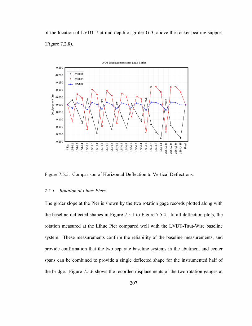
of the location of LVDT 7 at mid-depth of girder G-3, above the rocker bearing support
(Figure 7.2.8).
LVDT Displacements per Load Series
-0.250
-0.200
-0.150
-0.100
-0.050
0.000
0.050
0.100
0.150
0.200
0.250
Initi
al
LS1-
L1
LS1-
L2
LS1-
L4
LS2-
L1
LS2-
L2
LS2-
L4
LS3-
L1
LS3-
L2
LS3-
L4
LS4-
L1
LS4-
L2
LS4-
L4
LS5-
L1
LS5-
L2
LS5-
L4
LS6-
L1
LS6-
L2
LS6-
L3
LS6-
L4
LS6-
L1 R
LS6-
L2 R
LS6-
L3 R
LS6-
L4 R
Fina
l
Dis
plac
emen
t (in
)
LVDT01
LVDT05
LVDT07
Figure 7.5.5. Comparison of Horizontal Deflection to Vertical Deflections.
7.5.3 Rotation at Lihue Piers
The girder slope at the Pier is shown by the two rotation gage records plotted along with
the baseline deflected shapes in Figure 7.5.1 to Figure 7.5.4. In all deflection plots, the
rotation measured at the Lihue Pier compared well with the LVDT-Taut-Wire baseline
system. These measurements confirm the reliability of the baseline measurements, and
provide confirmation that the two separate baseline systems in the abutment and center
spans can be combined to provide a single deflected shape for the instrumented half of
the bridge. Figure 7.5.6 shows the recorded displacements of the two rotation gauges at
207
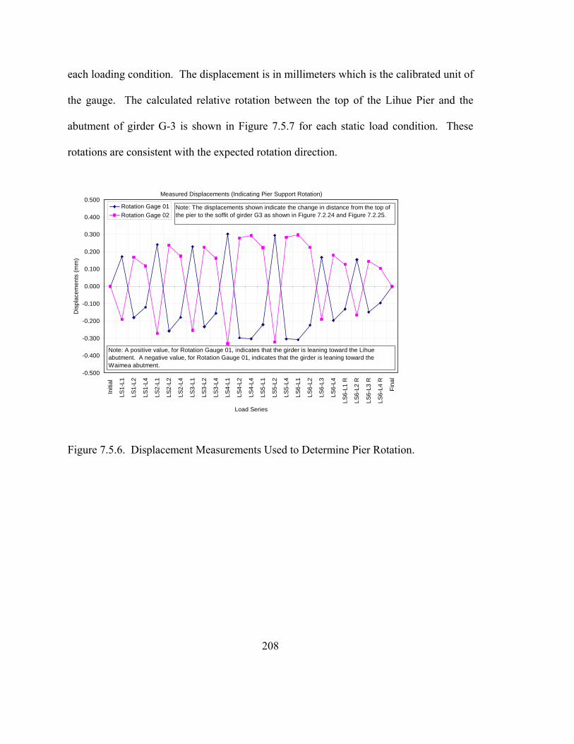
each loading condition. The displacement is in millimeters which is the calibrated unit of
the gauge. The calculated relative rotation between the top of the Lihue Pier and the
abutment of girder G-3 is shown in Figure 7.5.7 for each static load condition. These
rotations are consistent with the expected rotation direction.
Measured Displacements (Indicating Pier Support Rotation)
-0.500
-0.400
-0.300
-0.200
-0.100
0.000
0.100
0.200
0.300
0.400
0.500
Initi
al
LS1-
L1
LS1-
L2
LS1-
L4
LS2-
L1
LS2-
L2
LS2-
L4
LS3-
L1
LS3-
L2
LS3-
L4
LS4-
L1
LS4-
L2
LS4-
L4
LS5-
L1
LS5-
L2
LS5-
L4
LS6-
L1
LS6-
L2
LS6-
L3
LS6-
L4
LS6-
L1 R
LS6-
L2 R
LS6-
L3 R
LS6-
L4 R
Fina
l
Load Series
Dis
plac
emen
ts (m
m)
Rotation Gage 01Rotation Gage 02
Note: The displacements shown indicate the change in distance from the top of the pier to the soffit of girder G3 as shown in Figure 7.2.24 and Figure 7.2.25.
Note: A positive value, for Rotation Gauge 01, indicates that the girder is leaning toward the Lihue abutment. A negative value, for Rotation Gauge 01, indicates that the girder is leaning toward the Waimea abutment.
Figure 7.5.6. Displacement Measurements Used to Determine Pier Rotation.
208

Measured Rotation at the Lihue Pier
-0.03
-0.02
-0.01
0.00
0.01
0.02
0.03
Initi
al
LS1-
L1
LS1-
L2
LS1-
L4
LS2-
L1
LS2-
L2
LS2-
L4
LS3-
L1
LS3-
L2
LS3-
L4
LS4-
L1
LS4-
L2
LS4-
L4
LS5-
L1
LS5-
L2
LS5-
L4
LS6-
L1
LS6-
L2
LS6-
L3
LS6-
L4
LS6-
L1 R
LS6-
L2 R
LS6-
L3 R
LS6-
L4 R
Fina
l
Load Series
Dis
plac
emen
ts (d
egre
es)
Note: A positive value on this graph indicates that the girder is leaning toward the Lihue abutment. A negative value indicates that the girder is leaning toward the Waimea abutment.
Figure 7.5.7. Rotation of Lihue Pier.
7.5.4 Crack Mouth Opening Displacements
The crack mouth opening displacements were monitored during static and dynamic truck
loading conditions. The maximum extension of the existing cracks was found to be very
small and of no structural concern. The results are shown per span per load series in the
Figure 7.5.8 through Figure 7.5.10 below.
7.5.4.1 General
Girder G-3 has a number of flexural and shear cracks in all spans. Crack gages were
installed at 10 locations on selected cracks as described in Section 7.2.3. The largest
existing crack on girder G-3 was 0.025” (0.64 mm) wide, based on prior visual
inspections. Figure 7.5.8 shows the changes in crack width as recorded by all 10
209

electronic crack gages under each loading condition. Drawn on a scale of +/-0.02 inch
(+/-0.51 mm), it is clear that the changes in crack size are very small. Figure 7.5.9 shows
a magnified plot of the crack gage records.
Crack Width Changes
-0.020
-0.015
-0.010
-0.005
0.000
0.005
0.010
0.015
0.020
Initi
al
LS1-
L1
LS1-
L2
LS1-
L4
LS2-
L1
LS2-
L2
LS2-
L4
LS3-
L1
LS3-
L2
LS3-
L4
LS4-
L1
LS4-
L2
LS4-
L4
LS5-
L1
LS5-
L2
LS5-
L4
LS6-
L1
LS6-
L2
LS6-
L3
LS6-
L4
LS6-
L1 R
LS6-
L2 R
LS6-
L3 R
LS6-
L4 R
Fina
lLoad Series
Cha
nge
in C
rack
Wid
th O
peni
ng (i
n)
Crack Gage 01Crack Gage 02Crack Gage 03Crack Gage 04Crack Gage 05Crack Gage 06Crack Gage 07Crack Gage 08Crack Gage 09Crack Gage 10
Figure 7.5.8. Crack Gauge measurements per Load Series.
The largest crack opening recorded by any of the electronic crack gauges during all of the
loading conditions was 0.0014” (1.4 thousandths of an inch or 0.036 mm). This is an
extremely small change in crack width, which occurred at crack gauge 10, located over a
flexural crack in the soffit of the Lihue Abutment span. The existing crack size of 0.009”
(0.229 mm) therefore increased to 0.0104” (0.264 mm) under maximum loading on this
span (LS6-L1), before returning to its original size after removal of the truck load. All
other crack gauges recorded width changes less than one thousandth of an inch.
210

Crack Width Changes
-0.0020
-0.0015
-0.0010
-0.0005
0.0000
0.0005
0.0010
0.0015
0.0020
Initi
al
LS1-
L1
LS1-
L2
LS1-
L4
LS2-
L1
LS2-
L2
LS2-
L4
LS3-
L1
LS3-
L2
LS3-
L4
LS4-
L1
LS4-
L2
LS4-
L4
LS5-
L1
LS5-
L2
LS5-
L4
LS6-
L1
LS6-
L2
LS6-
L3
LS6-
L4
LS6-
L1 R
LS6-
L2 R
LS6-
L3 R
LS6-
L4 R
Fina
l
Load Series
Cha
nge
in C
rack
Wid
th O
peni
ng (i
n)
Crack Gage 01 Crack Gage 02Crack Gage 03 Crack Gage 04Crack Gage 05 Crack Gage 06Crack Gage 07 Crack Gage 08Crack Gage 09 Crack Gage 10
Figure 7.5.9. Crack Gauge Measurements per Load Series (Magnified).
Lihue Bound Crack Openings Dynamic
-0.00050
-0.00025
0.00000
0.00025
0.00050
0.00075
0.00100
5000 7000 9000 11000 13000 15000 17000 19000 21000 23000 25000
Time (ms)
Cra
ck o
peni
ng (i
n)
Crack Gage 01Crack Gage 02
Crack Gage 03Crack Gage 04Crack Gage 05Crack Gage 06Crack Gage 07Crack Gage 08Crack Gage 09
Crack Gage 10
Figure 7.5.10. Dynamic Crack Opening Plots.
211

212
Figure 7.5.10 shows the effect on crack mouth opening behavior due to Truck 1 traveling
Lihue bound at 25 mph (40 km/h). This indicates both the resolution and small
magnitude of the observed behavior. The largest magnitude is that of crack gauge 10
which is installed at the soffit in the shallowest portion of the girder across a flexural
crack.
7.5.5 Dynamic Response
In order to determine the effect of dynamic loading on the bridge, Truck 1 was driven
over the bridge in both directions at 25 mph. Figure 7.5.11 and Figure 7.5.12 show
vertical deflections recorded by the LVDT-Taut-Wire baseline systems, and the
horizontal deflection recorded by LVDT 7, while Truck 1 was driven over the bridge at
25 mph towards Lihue and towards Waimea, respectively. The maximum vertical
deflections measured during these dynamic tests were 0.014” downward at midspan of
the center span, and 0.0075” upward at midspan of the Lihue abutment span. These
deflections are similar to those observed during static load tests utilizing the same Truck
1 in either the upstream or downstream traffic lane (Figure 7.5.3). It was also noted that
LVDT 7 recorded similar horizontal deflections as observed during the static load tests
(Figure 7.5.5).

Lihue Bound Truck at 25 MPH
-0.15
-0.1
-0.05
0
0.05
0.1
0.15Time (20 seconds)
Def
lect
ion
(in)
LVDT01LVDT02LVDT03LVDT04LVDT05LVDT06LVDT07
Figure 7.5.11. Lihue Bound Dynamic Deflection at 25 mph.
Waimea Bound Truck at 25 MPH
-0.15
-0.1
-0.05
0
0.05
0.1
0.15Time (20 seconds)
Def
lect
ion
(in)
LVDT01LVDT02LVDT03LVDT04LVDT05LVDT06LVDT07
Figure 7.5.12. Waimea Bound Dynamic Deflection at 25 mph.
213

In order to determine whether the bridge was experiencing significant horizontal
movement longitudinal to the roadway, two dynamic tests were performed with Truck 1
breaking from 25 mph to zero while crossing the Lihue Pier. Figure 7.5.13 shows all
LVDT records during breaking of Truck 1 while Lihue bound. Figure 7.5.14 shows all
LVDT records during breaking of Truck 1 while Waimea bound. The horizontal
deflection recorded by LVDT 7 during both of these breaking tests show no indication of
additional deflection caused by the horizontal load. The sustained deflection occurred
while the truck was stationary after breaking, and prior to driving off the bridge. Apart
from the period while the truck was stationary, the vertical deflections recorded during
the breaking tests matched those recorded during the corresponding drive-through tests.
Lihue Bound Truck Breaking from 25 MPH
-0.15
-0.1
-0.05
0
0.05
0.1
0.15Time (40 seconds)
Def
lect
ion
(in)
LVDT01LVDT02LVDT03LVDT04LVDT05LVDT06LVDT07
Figure 7.5.13. Lihue Bound Dynamic Deflection Breaking From 25 mph.
214
Waimea Bound Truck Breaking from 25 MPH
-0.15
-0.1
-0.05
0
0.05
0.1
0.15Time (40 seconds)
Def
lect
ion
(in)
LVDT01LVDT02LVDT03LVDT04LVDT05LVDT06LVDT07
Figure 7.5.14. Waimea Bound Dynamic Deflection Breaking From 25 mph.
7.6 Conclusions about Bridge and SHM System
A diagnostic load test was performed on the bridge on July 19, 2005 to better understand
its strength and serviceability characteristics. A 3-dimensional computer model was used
as an analytical tool to help predict the bridge’s response to various loading conditions.
The model’s predictions were compared with field measurements. Based on the load test
results, the computer model was calibrated by adjusting the material property values. The
final calibrated computer model matched the bridge’s observed behavior very closely,
allowing for a more accurate load rating of the bridge.
The LVDT-Taut-Wire system has been used successfully for both short and long-term
static deflections using a manual reading system [Robertson et al. 2005, Chapter 3]. For
215

216
the Hanapepe Bridge application, the manual readings were replaced by automated
LVDTs because of limited access below the bridge, and to reduce the time required to
take readings. This automated system also allowed for dynamic tests to be performed
with a moving truck load. The Wheatstone Bridge based pin-rotation monitoring gauges
designed for this bridge performed well during this application as well. These gauges
provided the continuity of measurements across the Lihue Pier support; they confirmed
the overall displaced shape of the structure at all loading cases including the dynamic
cases. The Wheatstone bridge based crack gauges designed for this bridge performed
well during this application. The crack gauges showed that the instrumented crack are
active, however, they are well bridged by non-yielding reinforcing.

217
CHAPTER 8. OTHER PLANNED SHM IMPLEMENTATIONS
8.1 North Halawa Valley Viaduct (NHVV)
8.1.1 Background
The NHVV is a segmental cast-in-place post-tensioned concrete box-girder bridge.
Previously, the viaduct was instrumented for long-term monitoring of creep and
shrinkage behavior for this type of construction [Robertson & Ingham 1999]. The project
produced more knowledge about the unique constitutive properties of the local concrete
and allows for better design and performance analysis of future structures of this type.
The data obtained was used to calibrate computer models of the long term behavior of the
viaduct.
Instrumentation used during that structural monitoring project include: LVDTs, vibrating
wire strain gauges, electrical resistance strain gauges, demec strain gauges,
thermocouples, tiltmeters, extensometers, and load cells.
Using the NHVV as a test bed allows us to properly configure future SHM systems to
observe short and long-term deflection behavior and the effects of dynamic traffic
loading. During the course of the research described in this dissertation, the viaduct
structure was used as a test bed for components of a SHM system planned for installation
during the Kealakaha Stream Bridge Seismic Instrumentation Program. Specifically, the
LVDT-Taut-Wire baseline system was installed along one of the spans of the viaduct.
The observations obtained during the process are described in chapter 3. The most recent
218
iteration of the system provides reasonable vertical deflection results for long span
applications—some of the observations are shown below. Also, 12 one meter long strain
gauges were installed on one span of the viaduct to test the C2D method deflection
calculation. Some of the initial results and systematic implications for the method are
described here as well. The intent of both of these systems is to monitor a structural
response phenomenon to help determine the structural health of the structure. Another
SHM process that will be tested on the NHVV is real-time website publication of the test
bed application data.
8.1.2 Results: LVDT-Taut-Wire Baseline System
The following plots were acquired during a single day from the LVDT-Taut-Wire
baseline system. There are seven LVDTs attached to a single taut-wire baseline that
spans 345 ft (105m). The total pier to pier length of the monitored span is 360 ft (110m).
The data captured both truck loading and temperature-induced loading. The prior
instrumentation program determined that for this span the thermal-induced deflection
displaces downward as the top surface heats up and it displaces upward as it cools. This
is due to the boundary conditions of the adjacent spans. The LVDT-Taut-Wire system
captured this behavior as shown in Figure 8.1.1. Traffic-induced deflections were also
captured with the LVDT-Taut-Wire baseline system as shown in Figure 8.1.2. The figure
shows the result of two large trucks traveling down the viaduct in succession. From the
data, we can determine that the trucks were traveling at about 50 mph (80 km/h) and the
first truck was heavier that the second truck. Furthermore, the previous study showed

that a single HS-20 truck produces about a 0.25” deflection at midspan. If the system is
accurately providing the proper deflection, the trucks are likely close to the HS-20 size.
However, at this stage in development, it is prudent to calibrate an LVDT-Taut-Wire
baseline system with a load test to accurately evaluate the deflection results and
subsequently determine truck loads. A load test was not performed for this structure in
the course of the LVDT-Taut-Wire system development. However, the system was
observed in a side by side comparison with an optical survey as discussed in chapter 7.
-0.05
0
0.05
0.1
0.15
11:3
9 P
M
2:40
AM
5:41
AM
8:43
AM
11:4
4 A
M
2:44
PM
5:44
PM
8:42
PM
11:1
6 P
M
Time (24 hours total)
Def
lect
ion
at L
VD
T 5
(inch
)
Figure 8.1.1. Thermal Deflection Observed by an LVDT-Taut-Wire Baseline System.
219
-0.25
-0.2
-0.15
-0.1
-0.05
0
0.05
0.1
0 5 10 15 20 25 30 35 40
Time (seconds)
Def
lect
ion
(inch
)
LVDT 1LVDT 2LVDT 3LVDT 4LVDT 5LVDT 6LVDT 7
Figure 8.1.2. Traffic Loading Observed by an LVDT-Taut-Wire Baseline System.
8.1.3 Results: Strain Gauge Based C2D Methodology
A total of 12 electrical resistance based strain gauge devices were installed in a single
span of the NHVV at six curvature measurement locations. A C2D Model consisting of
two beam sections with a single node at mid span is currently under construction. Figure
8.1.3 shows data observed during a truck loading event. The data collected reveals that
curvature measurement location 3 occurred at an inflection point so no significant strain
change is observed. Also, a few of the six strain gauge devices mounted to the soffit of
the top slab on the box-girder are near the neutral axis; they do not observe significant
strain changes either. Both of these two observations are important to determining the
final configuration of a C2D based deflection measurement system. If the intent is to
measure traffic-induced deflections only, the low signal to noise ratio that exists at the
inflection point or neutral axis locations may only serve to generate signal errors in the
220
calculation of the deflection. A location with a larger signal to noise ratio may lesson the
overall noise.
-15
-10
-5
0
5
10
15
29:56 29:57 29:59 30:01 30:03 30:04 30:06 30:08 30:10 30:11 30:13
Time (minutes:seconds)
Stra
in (m
icro
stra
in) BOT-Location 1
TOP-Location 1
BOT-Location 2
TOP-Location 2
BOT-Location 3
TOP-Location 3
BOT-Location 4
TOP-Location 4
BOT-Location 5
TOP-Location 5
BOT-Location 6
TOP-Location 6
Figure 8.1.3. Strain Measurements from 1 m Long Gauges During Truck Loading
8.2 Kealakaha Stream Bridge Seismic Instrumentation
8.2.1 Background
This bridge was originally designed very similar to the NHVV. The method of
construction was originally planned to be a segmental cast-in-place post-tensioned
concrete box-girder bridge. The contractor who won the bid proposed a value engineered
(VE) design to include friction pendulum style base-isolation at the top of the piers and
abutments to save on foundation construction costs. This dramatically changes the
requirements of the SHM system.
221

222
The purpose of the SHM system is to observe the seismic response of the new, long,
three-span bridge. Short and long-term deflections will also be monitored. The
instrumentation that will be used in the SHM system includes: accelerometers, fiber optic
strain gauges for the C2D methodology, LVDTs, multiple LVDT-Taut-Wire baseline
systems, pull wire displacement transducers, tiltmeters, and GPS stations. Other
instrumentation systems yet to be developed may help to accommodate the change in
structural system as well. The final data products for this SHM system includes a real-
time web published report coupled with a database of observations from long-term and
short-term phenomena. The recording system will be triggered to record seismic events
at higher acquisition speeds.
8.2.2 LVDT-Taut-Wire Baseline System
Originally, three LVDT-Taut-Wire baseline systems were planned to measure the vertical
deflection of each of the three spans along the bridge. The baselines would have been
completely enclosed within the box section. However, the new design of the
superstructure is a multi-cell box girder/pre-cast beam composite. Along the box girder
section, each cell is much narrower than the original single box design. Since the
superstructure is curved, this limits the straight line distance that the LVDT-Taut-Wire
baseline can span without interfering with the webs of each cell. The planned single taut-
wire spanning from pier to pier will not work without cutting through the web of either a
pre-cast beam or a cell wall within the multi-cell box girder. The long middle span will
now need three taut-wire baselines to fit within the curved superstructure. The detail of

223
the connections between the box girder section and the pre-cast beam section also
restricts the placement of a single taut-wire baseline.
A total of five baselines need to be installed—complete with extra-baseline
measurements that capture rigid body displacements of the ends of each of the baseline
systems. In the original configuration an assumption of zero vertical displacement at the
end of the baseline span was used to calculate the total displacement of the superstructure
from the relative measurements observed by the LVDTs. Now, the relative
measurements recorded from the LVDTs will be with respect to a point that is within the
deflecting span. A new method to determine the relative vertical displacement of the
dead end or live end of the baseline needs to be developed. The vertical deflection
caused by the inverted pendulum base-isolation devices needs to be accounted for as
well. Each support is subject to this movement. A system of pull-wire displacement
transducers will be used to determine the three-dimensional motion of the superstructure
with respect to the top of the piers and abutments. The investigators hope to design a
system that is robust enough to identify any residual displacements that exist in a post
earthquake condition.
8.2.3 C2D Methodology
The original design of the Kealakaha Stream Bridge was only expected to see about a 40
microstrain change at mid span under typical traffic loading. This was large enough such
that the planned fiber optic strain gauges would produce a sufficient signal to noise ratio
to measure curvatures at various locations. The noise characteristics and observations of

224
C2D error propagation discussed in chapters 5 and 6 will be incorporated into the final
design. Constant beam section properties are an assumption of the C2D method, so, an
exact solution was not possible for the original design of the system without a different
form of the estimate curvature function. Alternate formulations are under consideration
to obtain the best formulation to encompass the various expected loading conditions.
However, due to the new VE structural system, first a new finite element structural
analysis needs to be performed to identify the new locations to place the strain gauges.
The new design with its much more complex geometry, requires an additional, and likely
multiple, curvature estimate formulations to be applied to the C2D algorithm. The fiber
optic strain measurements used will need to be observed at many more locations to
properly reflect the change in beam section properties between the box girder and pre-
cast beam sections. The load sharing between the pre-cast beams will need to be
accounted for more closely than the previous box girder design would have required.
The instantaneous change in stiffness along the spans will alter mode shapes of the
structure. The error analysis in this dissertation shows that the more curvature
measurement locations incorporated into the C2D model, the larger the error away from
the prescribed boundary conditions. If indeed the new structural system needs more
curvature measurement locations to accurately determine the deflection of the
superstructure, it may prove to be too difficult to obtain an accurate displacement
configuration during dynamic events without a much faster acquisition speed and some
data averaging techniques.

225
8.3 Salt Lake Boulevard – Halawa Stream Bridge: Shear Retrofit
8.3.1 Background
The Salt Lake Boulevard-Halawa Stream Bridge has multiple shear cracks in several of
its beams. The retrofit process will include epoxy injection crack repair and two shear
capacity upgrades. The Engineer of Record for the repair chooses to use a classic steel
rod and plate shear retrofit technique at the most critical locations. A shear retrofit
technique using carbon fiber reinforced polymer (CFRP) will be applied at other
locations which are heavily loaded compared to their calculated capacity.
Since the CFRP technique is relatively new, a SHM program intended to monitor the
structural health of the CFRP retrofit is underway. The phenomenon which will be
measured is the strain level in the CFRP fabric. One of the possible failure modes that is
of concern to the owner is the brittle sliding mode crack propagation that occurs between
the concrete substrate and the CFRP during debonding. The concern is that this mode
two sliding fracture type brittle failure will be induced by crack mouth opening
displacements at existing shear cracks. This type of failure mode was investigated in the
University of Hawaii’s materials testing lab. It is thought that by observing strain in the
CFRP at the region that is susceptible to crack formation, the initiation of debonding
failure may be detectable.
8.3.2 Planned Instrumentation
The SHM system is designed to use fiber Bragg grating (FBG) fiber optic strain gauges
to monitor the strain in the CFRP. The system will be designed and calibrated to observe

226
traffic induced straining of the material. It is hoped that a relationship between observed
loading and possible deterioration of the retrofit can be detected—if failure begins.
This project is an excellent case study to observe all the SHM issues relating to the
practical implementation of a real-time remote instrumentation project. The strain
measurements require no heavy mathematics to analyze the current structural health.
Because it is a relatively simple system, the budget is also small. At some time in the
future, cracks may develop in the concrete near the retrofit. The economically designed
Wheatstone bridge based crack gauges discussed in chapter 4 could be easily
incorporated at that time for relatively little effort. This will provide another bit of
information to help determine the cause of any deterioration in the structural health of the
retrofit schemes used.

227
CHAPTER 9. SUMMARY AND CONCLUSIONS
In this age of computers and electronics, we become increasingly aware of all the new
information we can collect about our surroundings. The medical industry has fully
embraced the use of this technology to help diagnose problems with our health. Better
diagnosis leads to appropriate and effective treatment when there is a problem. The
result is that we are living longer, more productive lives. The structural engineering
profession is only now beginning the steps toward the promise of extending the
productive lives of our infrastructure using structural health monitoring (SHM).
The education of structural engineering professionals does not yet incorporate SHM
system design into its curriculum. To help open the instrumentation world to engineers
and scientists, an example of the process by which to design an economical crack gauge
was discussed. While the technology used for that gauge is not new, it does provide an
economical and robust alternative to other devices. The device has performed well
during the Hanapepe River Bridge Load Test as discussed in Chapter 7.
The new contributions developed during the course of this research include: (1) a simple
design process for an LVDT-Taut-Wire baseline system that measures vertical
deflections on long and short span beams; and (2) a method by which to determine the
expected error caused by real data for a strain based deflection monitoring algorithm
(C2D Method). Both of these contributions will help to more quickly design such
systems and have reasonable confidence of their performance before they are installed.
Specific conclusions about the two systems are listed below.

228
The following conclusions about the LVDT-Taut-Wire baseline system and presented
design process have been established.
• The proposed system is viable for monitoring static, diurnal, and traffic induced
vertical deflections of beams.
• The system can work for both short- and long-span bridges.
• The initial sizing of the system can be accomplished by a design process using a
simple “Rule of Thumb” procedure.
• An initial estimate of error can be determined or set during the design process.
The following conclusions about the C2D Method and presented analysis of the process
have been established.
• Using a second degree polynomial to represent the curvature function in a beam
provides excellent results when the applied loads conform to the exact solution: (1) point
loads are applied at the nodes between (and / or at the ends of) beam sections; and (2)
uniformly distributed loads act along the entire length of a beam section.
• Using a second degree polynomial for the curvature function can also produce
good results in some cases even for non-conforming applied loads such that curvature
measurement resolution is sufficient—with enough significant figures.
• Inadequate curvature measurement resolution can produce much larger error than
non-conforming loading configurations, because: (1) more beam sections are affected,

229
and (2) the error is integrated twice over a longer span of the beam than a non-
conforming load-induced curvature function in one beam section.
• Signal noise characterization is a useful tool to determine the expected range of
error in a C2D modeled system.
• Displacement errors tend to increase with distance from prescribed boundary
conditions within the C2D modeled beam.
• Data averaging techniques will likely improve the performance of the C2D
method results from a dynamically acquired signal. This is necessary to effectively
determine structural characteristics including: natural frequency, damping ratio, and
mode shape.
Finally, the four SHM projects described in this dissertation will benefit from the analysis
and results reported to date. Each project has different phenomena to be monitored;
different combinations of instrumentation used; and different data products to be
produced. It is important to continue the discussion of lessons learned in SHM successes
and failures to advance the field by developing more easily available and useful tools for
engineers and owners of infrastructure.

230

231
APPENDIX
A5.4 Matlab™ C2D Method Computer Program...................................................... 233
A8.2 Crack Gauges: Supplementary Figures.............................................................. 245
A8.4 Truck Loading Series ......................................................................................... 251

232

233
A5.4 Matlab™ C2D Method Computer Program
This Matlab™ program is structured such that the main program performs function calls
to the other program files. The dependency and function of each file is described below.
• main.m retrieves the input data from the input text file, it sends the data to the
C2D() function. It saves the output data to the output file and sends the data to
the function plotter3d().
• C2D.m is the function that contains the algorithm for the C2D method. C2D.m
prepares the data for the calculation of the curvature function coefficients a, b,
and c—by calling the function element_defl(). Upon receiving the a, b, and c
coefficients matrix, it calculates the rotation and displacements for the entire
beam for all the time steps requested.
• element_defl.m is the function that is given the curvature and strain gauge
location data and returns the a, b, and c coefficients matrix. It calls the function
Gauss() to solve the linear system of equations for a, b, and c.
• Gauss.m is a general Gaussian elimination linear system of equations solver.
• plotter3d.m plots the output file array as a surface and contour plot of all the data
versus time.
• main_noise.m retrieves the input data from the input file, then it augments that
data with errors of a specified magnitude and sends the new data set to the C2D()

function. It saves the data with error to a new file per error level and plots the
data.
The Programs are listed below in the following order: main.m, C2D.m, element_defl.m,
Gauss.m, plotter3d.m, main_noise.m.
main.m
234

C2D.m
235

236

237

238

239

element_defl.m
240

Gauss.m
241

plotter3d.m
242

main_noise.m
243

244

A8.2 Crack Gauges: Supplementary Figures
Figure A8.2.17. Crack Gauges 1 (Left) and 2 Adjacent to Visual Crack Monitor 19
(Right), Shear Cracks.
245
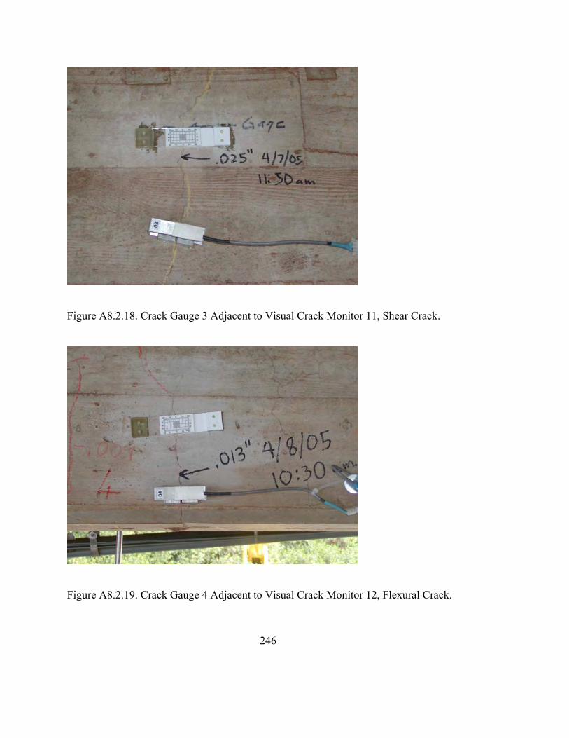
Figure A8.2.18. Crack Gauge 3 Adjacent to Visual Crack Monitor 11, Shear Crack.
Figure A8.2.19. Crack Gauge 4 Adjacent to Visual Crack Monitor 12, Flexural Crack.
246

Figure A8.2.20. Crack Gauge 5 Adjacent to Visual Crack Monitor 13., Flexural Crack.
Figure A8.2.21. Crack Gauge 6, Shear Crack.
247

Figure A8.2.22. Crack Gauge 7, Shear Crack.
Figure A8.2.23. Crack Gauge 8 Adjacent to Visual Crack Monitor 2, Shear Crack.
248

Figure A8.2.24. Crack Gauge 9 Adjacent to Visual Crack Monitor 3, Shear Crack.
Figure A8.2.25. Crack Gauge 10 Adjacent to Visual Crack Monitor 12, Flexural Crack.
249

250

A8.4 Truck Loading Series
Figure A8.4.3. Load Series 1 – Location 1 (LS1-L1).
Figure A8.4.4. Load Series 1 – Location 2 (LS1-L2).
251

Figure A8.4.5. Load Series 1 – Location 4 (LS1-L4).
Figure A8.4.6. Load Series 2 – Location 1 (LS2-L1).
252
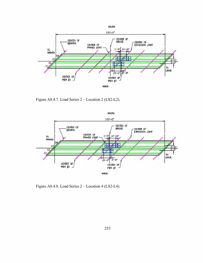
Figure A8.4.7. Load Series 2 – Location 2 (LS2-L2).
Figure A8.4.8. Load Series 2 – Location 4 (LS2-L4).
253
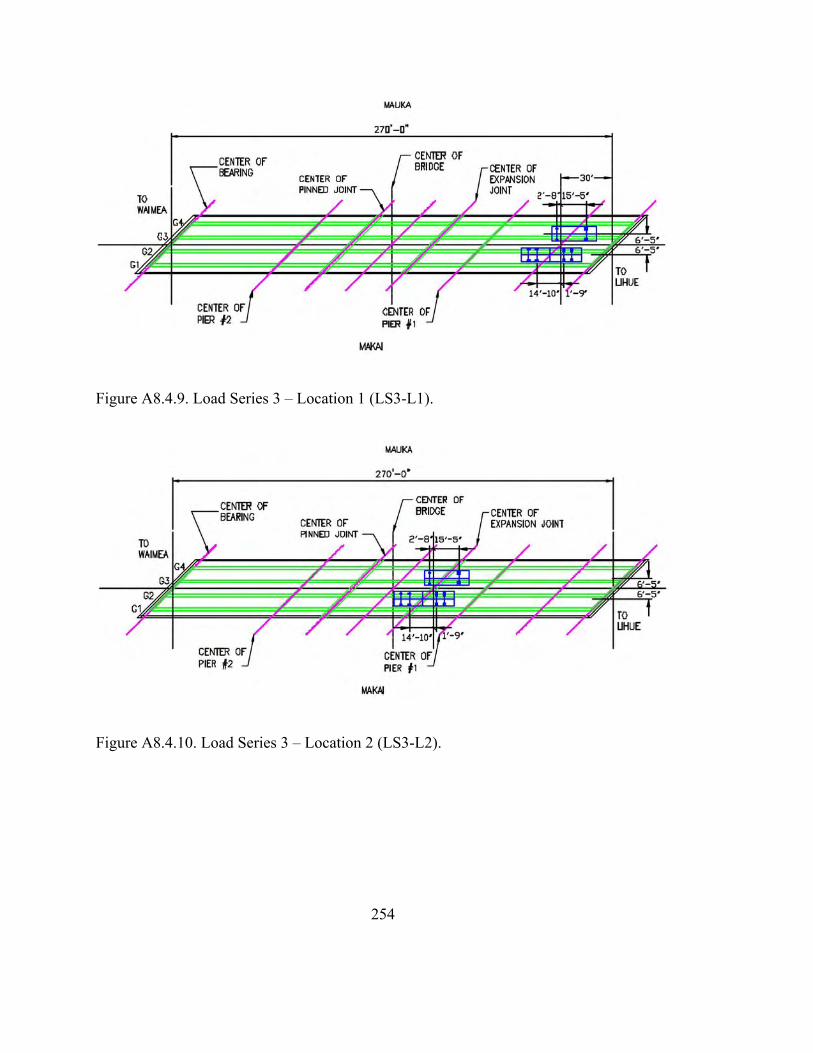
Figure A8.4.9. Load Series 3 – Location 1 (LS3-L1).
Figure A8.4.10. Load Series 3 – Location 2 (LS3-L2).
254

Figure A8.4.11. Load Series 3 – Location 4 (LS3-L4).
Figure A8.4.12. Load Series 4 – Location 1 (LS4-L1).
255
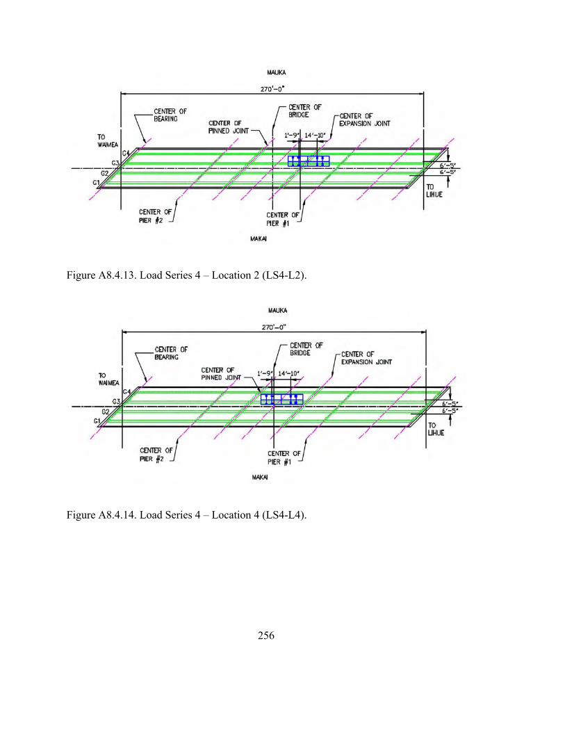
Figure A8.4.13. Load Series 4 – Location 2 (LS4-L2).
Figure A8.4.14. Load Series 4 – Location 4 (LS4-L4).
256
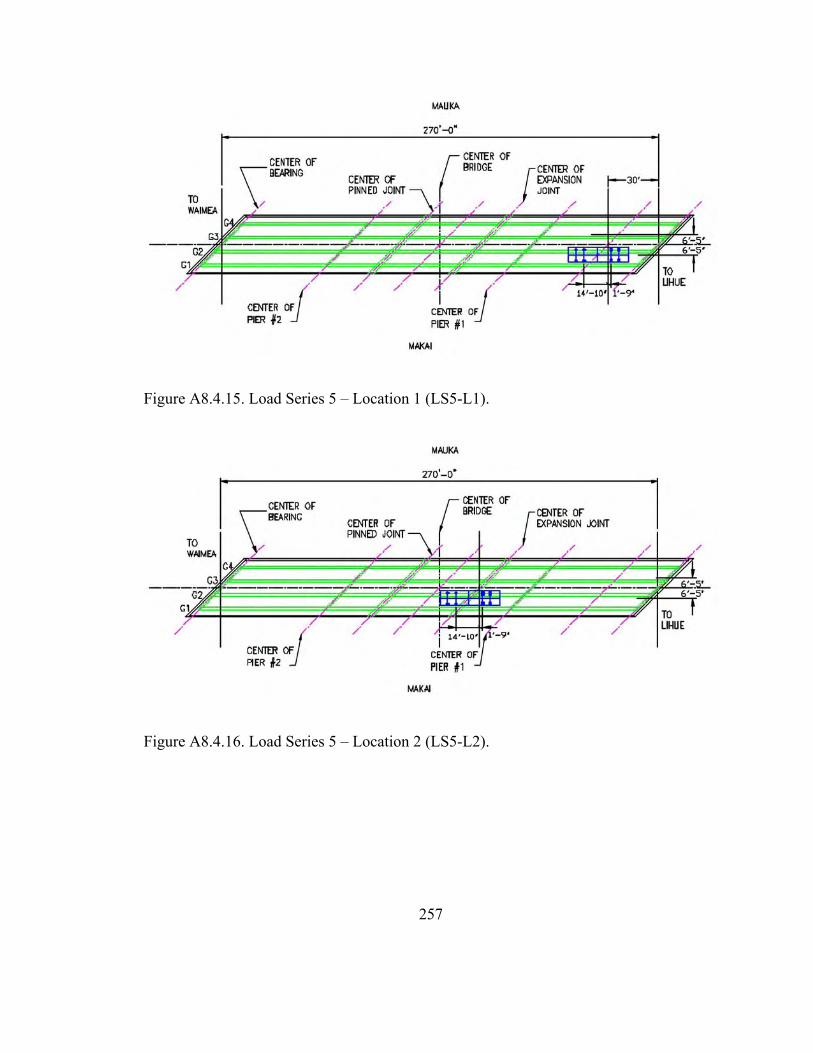
Figure A8.4.15. Load Series 5 – Location 1 (LS5-L1).
Figure A8.4.16. Load Series 5 – Location 2 (LS5-L2).
257

Figure A8.4.17. Load Series 5 – Location 4 (LS5-L4).
Figure A8.4.18. Load Series 6 – Location 1 (LS6-L1).
258

Figure A8.4.19. Load Series 6 – Location 2 (LS6-L2).
Figure A8.4.20. Load Series 6 – Location 3 (LS6-L3).
259

Figure A8.4.21. Load Series 6 – Location 4 (LS6-L4).
260

261
REFERENCES
[Agapay & Robertson 2004] Agapay, Alison & Robertson, Ian N. “Test of Prestressed
Concrete T-Beams Retrofitted for Shear and Flexure Using Carbon Fiber
Reinforced Polymers,” Research Report UH/CEE/04-08, University of Hawaii,
Honolulu, HI, USA, 268 p.
[Aki & Robertson 2005] Aki, Kainoa D. & Robertson, Ian N. “Deflection Monitoring
Systems in Static and Dynamic Conditions,” Research Report UHM/CEE/05-02,
University of Hawaii, Honolulu, HI, 71 p.
[Aktan et al. 2002] Aktan, A. E., Catbas, F. N., Grimmelsman, K.A., & Pervizpour, M.
“Development of a Model Health Monitoring Guide for Major Bridges”, Drexel
Inteligent Infrastructure and Transprotation Safety Institute, Federal Highway
Administration, Research and Development, Contract/Order No. DTFH61-01-P-
00347, 270 p.
[Aktan et al. 2003] Aktan, A. E., Catbas, F. N., Grimmelsman, K.A., & Pervizpour, M.
“Development of a Model Health Monitoring Guide for Major Bridges,” Drexel
Intelligent Infrastructure & Transportation Safety Institute, Drexel University,
2003, pg D3-D4.
[Basu & Knickerbocker 2005] Basu, P. K. & Knickerbocker, D. J., “Behavior of Jointless
High Performance Concrete Bridges,” Final Report Project Number TNSPR-

262
RES1162, State of Tennessee, DOT, USDOT, FHA, Vanderbilt University,
Nashville, TN, USA.
[Bergmeister 2002] Bergmeister, Konrad., “Monitoring and Safety Evaluation of Existing
Concrete Structures: State-of-the-Art Report”, fib Task Group 5.1, Final Draft.
[Bohnhoff et al. 1997] Bohnhoff, D. R., Chiou, W., & Hernandez, R., “Load Sharing in
Nail-Laminated Assemblies Subjected to Bending Loads,” Presented at the
August 10-14 1997 ASAE Annual International Meeting. Paper No. 974090.
ASAE, St Joseph, MI USA, pg. 9.
[Chiareli 1999] Chiareli, Alessandra., Fiber Optics & Electronics Technology Center,
3M. Lecture Webpage: http://www.ima.umn.edu/talks/workshops/9-9-10.99/
chiareli/ chiareli.pdf.
[Cho et al. 2000] Cho, N., Kim, N., Jang, J., & Chang, S., “Estimation of deflection
curve of bridges using fiber optic strain sensors,” Proc. SPIE Vol. 3988, pg. 339-
348.
[Drexel 2006] Drexel University Website: http://repairfaq.ece.drexel.edu/sam/
CORD/loet/ cource10_mod5/ mod10-05.html.
[Fausett 1999] Fausett, L. V., Applied Numerical Analysis using Matlab®, Upper Saddle
River, NJ: Prentice Hall, 596 p.

263
[Ferreira et al. 2000] Ferreira, L. A., Araujo, F. M., Santos, J. L., & Farahi, F.,
“Simultaneous measurement of strain and temperature using interferometrically
interrogated fiber Bragg grating sensors,” Opt. Eng., Vol. 39, No. 8, August, pg.
2226-2234.
[Fiso 2006] Fiso Technologies Inc. Website: http://www.spie.org/web/oer/october/oct98/
fiberop.html
[Fraden 2004] Fraden, J., ed. Handbook of Modern Sensors: Physics, Designs, and
Applications, 3rd ed., New York: Springer.
[Fung & Robertson 2003] Fung, S. S. Y., & Robertson, I. N. “Seismic Monitoring of
Dynamic Bridge Deformations Using Strain Measurements,” Research Report
UHM/CEE/03-02 University of Hawaii, Honolulu, HI, 112 p.
[Hansen & Condon 1989] Hansen, Gladys, & Condon, Emmet, Denial of Disaster: The
untold story and photographs of the San Francisco earthquake and fire of 1906,
San Francisco: Cameron and Co. 160 p.
[Harris & Piersol 2002] Harris, C. M. & Piersol, A. G., eds. Harris’ Shock and Vibration
Handbook , 5th ed. New York: McGraw-Hill.
[Henriksson et al. 1996] Henriksson, A., Sandgren, S., & Asseh, A., “Temperature
insensitivity of a fiber optic Bragg grating sensor,” Proc. SPIE Vol. 2839, pg20-
33

264
[Hernandez et al. 2005] Hernandez, R., Green, D. W., Kretschmann, D. E., & Verrill, S.
P. “Improved Utilization of Small-Diameter Ponderosa Pine in Glulam Timber,”
Research Paper FPL-RP-625. Madison, WI: U.S. Department of Agriculture,
Forest Service, Forest Products Laboratory, 38 p. (pg 10).
[Inaudi et al. 1998] Inaudi, D., Vurpillot, S., Casanova, N., & Kronenberg, P., “Structural
monitoring by curvature analysis using interferometric fiber optic sensors,” Smart
Mater. Struct. 7, pg 199-208.
[ISIS Canada 2001] ISIS Canada, “Guidelines for Structural Health Monitoring: Design
Manual No. 2”, ISIS Canada Corporation, University of Manitoba, Winnipeg,
Manitoba, Canada,. 127 p.
[Land et al. 2003] Land, R., Murugesh, G., & Raghavendrachar, M., “Assessing Bridge
Performance—When, What, How,” A Paper Presented to the 19th US-Japan
Bridge Engineering Workshop, Session 7, October 28 2003, Public Works
Research Institute, Tsukuba, Japan, pg 5-6.
[Lee & Robertson 1995] Lee, Andre, and Robertson, Ian N., “Instrumentation and Long-
Term Monitoring of the North Halawa Valley Viaduct,” Report UHM/CE/95-08,
University of Hawaii, Honolulu, Hawaii.
[Li & Robertson 2003] Li, X. and Robertson, I. N., “Long-Term Performance Predictions
of the North Halawa Valley Viaduct,” Research Report UHM/CEE/03-04,
University of Hawaii, Honolulu, Hawaii, 87p.

265
[Lopez-Higuera 2005] Lopez-Higuera, J. M., Misas, C. J., Incera, A. Q., Cuenca, J. E.,
“Fiber optic civil structure monitoring,” Optical Engineering, Vol. 44, No. 4,
Paper 044401, April, 10 p.
[Meltz 1996] Meltz, G., “Overview of Fiber Grating-Based Sensors,” Proc. SPIE Vol.
2838, pg. 2-22.
[Mufti et al. 2005] Mufti, A. A., Bakht, B., Tadros, G., Horosko, A. T., & Sparks, G.,
“Are Civil Structural Engineers ‘Risk Averse’? Can Civionics Help?,” Report
printed in Sensing Issues in Civil Structural Health Monitoring, Ed. Farhad
Ansari. Dordrecht, Netherlands: Springer, pg 3-12.
[Myers & Yang 2005] Myers, J., Yang, Y., “High Performance Concrete Bridge A6130-
Route 412 Pemiscot County, MO,” Report Number UTC R39, Center for
Infrastructure Engineering Studies/UTC Program, University of Missouri—Rolla,
Rolla, Missouri, pg 17, 65-66, 82.
[Nawy 2000] Nawy, Edward G., Prestressed Concrete : a Fundamental Approach, 3rd ed.
Upper Saddle River, New Jersey: Prentice-Hall. 466 p.
[NI 2000] National Instruments, SCXI™ - SCXI-1540 User manual: 8-Channel LVDT
Signal Conditioner, Austin, Texas: National Instruments, 70 p.
[NI 2006] National Instruments Website: http://www.ni.com.

266
[NOAA 1972] NOAA (National Oceanic and Atmospheric Administration), 1972, “A
study of earthquake losses in the San Francisco Bay Area - Data and Analysis,” A
report prepared for the Office of Emergency Preparedness: U.S. Department of
Commerce, 220 p.
[Norton 1989] Norton, H. N., Handbook of Transducers, Englewood Cliffs, NJ: Prentice
Hall. 554 p.
[Rao et al. 2002] Rao, Y.J., Yuan, S.F., Zeng, X.K., Lian, D.K., Zhu, Y., Wang, Y.P.,
Huang, S.L., Liu, T.Y., Fernando, G.F., Zhang, L., & Bennion, I., “Simultaneous
strain and temperature measurement of advanced 3-D braided composite materials
using an improved EFPI/FBG system,” Optics and Lasers in Engineering, Vol.
38, pg 557-566.
[Ravet et al. 2005] Ravet, F., Zou, L., Bao, X., Chen, L., Huang, R.F., & Khoo, H. A.,
“Pipeline Buckling Detection by the Distributed Brillouin Sensor,” Report printed
in Sensing Issues in Civil Structural Health Monitoring, Ed. Farhad Ansari.
Dordrecht, Netherlands: Springer, pg. 515-524.
[Reasenberg 2000] Reasenberg, Paul. “1906 Marked the Dawn of the Scientific
Revolution” U.S. Geological Survey, Earthquake Hazards Program Website:
http://quake.wr.usgs.gov/info/1906/revolution.html. August 14.

267
[Robertson & Ingham 1999] Robertson, Ian N. and Ingham, Tim., “Instrumentation of the
North Halawa Valley Viaduct Oahu, Hawaii Final Report,” Funded by the Hawaii
Department of Transportation and the U.S. Federal Highways Administration.
[Robertson & Yoshimura 2004] Robertson, I. N. & Yoshimura, R. K., “North Halawa
Valley Viaduct Load Test,” Research Report UHM/CEE/04-02, University of
Hawaii, Honolulu, Hawaii. 227 p.
[Robertson et al. 2005] Robertson, I. N., Johnson, G. P., and Wang, S., “Instrumentation
Performance during Long-Term Bridge Monitoring,” Report printed in Sensing
Issues in Civil Structural Health Monitoring, Ed. Farhad Ansari. Dordrecht,
Netherlands: Springer, pg 331-340.
[Salas 1995] Salas, S. L., Salas and Hille’s Calculus: One and Several Variables, 7th
edition, Ed. Garret Etgen. New York: John Wiley& Sons Inc. pg 888.
[Stanton et al. 2003] Stanton, J. F., Eberhard, M. O., & Barr, P. J., “A weighted-strethed-
wire system for monitoring deflections,” Engineering Structures Vol. 25, pg. 347-
357.
[Techkor 2001] Techkor Instrumentation, Inc., “Technical Brief TB-31, LVDT Basics-
An introduction to the Linear Variable Differential Transformer,” Middletown,
PA, USA: Advanced Conversion Technology, Inc., 3 p.

268
[Trietily 1986] Trietily, H. L., Transducers in Mechanical and Electronic Design, New
York: Marcel Dekker, Inc. 374 p.
[Virginia DOT 2006] Virginia Department of Transportation. “Virginia Test Method—
20,” Virginia Test Methods. http://www.virginiadot.org/business/resources/bu-
mat-VTMs070704.pdf. Accessed September 18, 2006.
[Vishay 2005] Vishay Micro-Measurments, “Strain Gage Thermal Output and Gage
Factor Variation with Temperature Technical Note TN-504-1,” Vishay Document
Number 11054, 13 p.
[Vishay 2006] Vishay Measurements Group Website: http://www.vishay.com/ brands/
measurements_group/ guide/tn/tn504/504j.htm.
[Vurpillot et al 1998] Vurpillot, S., Krueger, G., Benouaich, D., Clement, D., Inaudi, D.,
“Vertical Deflection of a Pre-Stressed Concrete Bridge Obtained Using
Deformation Sensors and Inclinometer Measurements,” ACI Structural Journal,
Vol. 95, No. 5, September – October Issue, pg. 518-526.
[Wnuk 2005] Wnuk, V. P., Mendez, A., Ferguson, S., Graver, T., “Process for Mounting
and Packaging of Fiber Bragg Grating Strain Sensors for use in Harsh
Environment Applications,” Proc. SPIE Paper 5758-6. 8 p.

269
[Zepernick & Finger 2005] Zepernick, H. & Finger, A., Pseudo random Signal
Processing: Theory and Application, San Francisco, CA, USA: John Wiley &
Sons. 414 p.
[Zhu et al. 2003] Zhu, Y., Shum, P., Lu, C., Lacquet, M. B., Swart, P.L., Chtcherbakov,
A. A., & Spammer, S. J., “Temperature insensitive measurements of static
displacements using a fiber Bragg grating,” Optics Express Vol. 11, No. 16,
August 11, pg. 1918-1924.