University of Groningen Application of the Maxwell–Stefan

University of Groningen

Application of the Maxwell–Stefan theory to the membrane electrolysis process. Modeldevelopment and simulationsHogendoorn, J.A.; Veen, A.J. van der; Stegen, J.H.G. van der; Kuipers, J.A.M.; Versteeg,G.F.Published in:Computers and Chemical Engineering

IMPORTANT NOTE: You are advised to consult the publisher's version (publisher's PDF) if you wish to cite fromit. Please check the document version below.

Document VersionPublisher's PDF, also known as Version of record

Publication date:2001

Link to publication in University of Groningen/UMCG research database

Citation for published version (APA):Hogendoorn, J. A., Veen, A. J. V. D., Stegen, J. H. G. V. D., Kuipers, J. A. M., & Versteeg, G. F. (2001).Application of the Maxwell–Stefan theory to the membrane electrolysis process. Model development andsimulations. Computers and Chemical Engineering, 25(9), 1251-1265.

CopyrightOther than for strictly personal use, it is not permitted to download or to forward/distribute the text or part of it without the consent of theauthor(s) and/or copyright holder(s), unless the work is under an open content license (like Creative Commons).

The publication may also be distributed here under the terms of Article 25fa of the Dutch Copyright Act, indicated by the “Taverne” license.More information can be found on the University of Groningen website: https://www.rug.nl/library/open-access/self-archiving-pure/taverne-amendment.

Take-down policyIf you believe that this document breaches copyright please contact us providing details, and we will remove access to the work immediatelyand investigate your claim.

Downloaded from the University of Groningen/UMCG research database (Pure): http://www.rug.nl/research/portal. For technical reasons thenumber of authors shown on this cover page is limited to 10 maximum.

https://research.rug.nl/en/publications/application-of-the-maxwellstefan-theory-to-the-membrane-electrolysis-process-model-development-and-simulations(36cf3793-757c-4dcb-b64e-55bf0fccad47).html

Computers and Chemical Engineering 25 (2001) 1251–1265

Application of the Maxwell–Stefan theory to the membraneelectrolysis process

Model development and simulations

J.A. Hogendoorn a,b, A.J. van der Veen a,1, J.H.G. van der Stegen a, J.A.M. Kuipers a,b,G.F. Versteeg a,b,*

a AKZO-Nobel Central Research B.V., RTB department, P.O. Box 9300, 6800 SB SB Arnhem, The Netherlandsb Department of Chemical Engineering, Uni�ersity of Twente, P.O. Box 217, 7500 AE Enschede, The Netherlands

Received 11 April 2000; received in revised form 1 March 2001; accepted 1 March 2001

Abstract

A model is developed which describes the mass transfer in ion-selective membranes as used in the chloralkali electrolysisprocess. The mass transfer model is based on the Maxwell–Stefan theory, in which the membrane charged groups are consideredas one of the components in the aqueous mixture. The Maxwell–Stefan equations are re-written in such a way that the currentdensity can be used as an input parameter in the model, which circumvents an extensive numerical iterative process in thenumerical solution of the equations. Because the Maxwell–Stefan theory is in fact a force balance, and the clamping force neededto keep the membrane charged groups in its place is not taken into account, the model is basically over-dimensioned: the molefraction of the membrane can be calculated by using the equivalent weight (EW) of the membrane or by using the equations ofcontinuity. In this work, the latter method has been chosen. The results of the computer model were verified in several ways,which show that the computer model gives reliable results. Several exploratory simulations have been carried out for a sulfoniclayer membrane and the conditions as encountered in the chloralkali electrolysis process. As there are no (reliable) Maxwell–Ste-fan diffusivities available for a Nafion membrane, in this trend study the diffusivities were all chosen equal at a more or lessarbitrary value of 1.10−10 m2 s−1. Due to this, the absolute values of several performance parameters are incorrect as comparedwith industrial chloralkali operation (e.g. an unrealistically high current efficiency of 95.7% was found), but the model can stillbe used to obtain trends. For example, it is shown that the thickness of the membrane hardly increases the current efficiency (CE),however, the required potential drop proportionally increases with thickness. The pH rapidly increases to values greater than 12just inside the membrane at the anolyte side. Moreover, for different values of the pH in the anolyte, the pH profiles inside themembrane nearly coincide with each other. A change in the anolyte strength does not have a significant effect on the performanceof the membrane. At low values of the current density, a high value of the current efficiency is found. However, this is not dueto a low OH− counter flux, but to the simultaneous transport of OH− and Cl− towards the catholyte. © 2001 Elsevier ScienceLtd. All rights reserved.

Keywords: Maxwell–Stefan theory; Membrane electrolysis process; Mass transfer

Nomenclature

A matrix with non-idealities, transference numbers and diffusivities (mol m−1 s−1)mass transfer parameter (follows from (Bn*)−1(�)) (mol m−1 s−1)Ai,j

Bn* matrix with diffusivities (s m mol−1)

www.elsevier.com/locate/compchemeng

* Corresponding author. Tel.: +31-53-4894337; fax: +31-53-4894774.E-mail address: [email protected] (G.F. Versteeg).1 Present address: Shell Moerdijk, The Netherlands.

0098-1354/01/$ - see front matter © 2001 Elsevier Science Ltd. All rights reserved.PII: S 0 0 9 8 -1354 (01 )00697 -4

J.A. Hogendoorn et al. / Computers and Chemical Engineering 25 (2001) 1251–12651252

Bi,j coefficient with electrical and mass transfer parameters (s m mol−1)transport coefficient (s m mol−1)Bi,j

n

Bi,jn * modified transport coefficient (s m mol−1)

current efficiency (− )CECD current density (A m−2)

concentration of component i (mol m−3)ci

cT total concentration (mol m−3)driving force of component i (J m−4)di

Ði,j binary Maxwell–Stefan diffusivity (m2 s−1)Faraday constant (96487 C mol−1) Coulomb mol−1)F

I current density (Coulomb m2 s−1)molar diffusive flux with respect to component n (mol m−2 s−1)Ji

n

friction coefficient (Js m−5)Ki, j

inverted transport coefficient (follows from the inverse of (Mn)) (m5 J s−1)Li,jn

Mi,j modified transport coefficient (follows from (K)) (J s m−5)modified transport coefficient ((M) without the nth row and column) (J s m−5)Mi, j

n

Ni molar flux of component i (mol m−2 s−1)total number of components (− )n

P pressure (Pa)universal gas constant (8.314413 J mol−1 K−1) (J mol−1 K−1)Rtemperature (K)Ttransference number of component i with respect to component n (− )t i

n

�i velocity of component i (m s−1)mole fraction of component i (− )xi

electrical coefficient (1 m−1)Zi

electrical coefficient (s m mol−1)Zi*electrical coefficient (Coulomb sm−1)Zi,j

c

zi ionic charge of component i (− )

Greek�i mass transfer parameter (follows from [Bn*]−1(Z*)) (mol Coulomb m−2)

mass transfer parameter (follows from [Bn*][Zc]) (mol m−2 s−1)�i,j�i,j thermodynamic factor (− )

activity coefficient of component i (− )�i

�i,j Kronecker-delta (�i, j=1 for i= j and �i, j=0 for i� j ) (− )electrical potential (mol m−3)�

conductivity (1 � m−1)�

electrochemical potential of component i (mol m−3)�i

� io chemical potential of component i in the reference state (mol m−3)

chemical potential of component i (mol m−3)� ichemical

factor consisting of transport and thermodynamic factors (− )�i,j

factor consisting of transport and thermodynamic factors (− )�i,j*

Sub/superscriptcomponent index or index of vector/matrixicomponent index or index of vector/matrixj

n nth component

Mathematical( ) vector

matrix[ ][ ]−1 inverse of a square matrix

gradient�Bold vectorial quantity(�x) divergence of a vector field

J.A. Hogendoorn et al. / Computers and Chemical Engineering 25 (2001) 1251–1265 1253

1. Introduction

Chlorine is one of the world’s most important chem-icals and is used not only to produce (consumer) endproducts, but also to produce a large amount of chlori-nated intermediate products as applied in e.g. organicsubstitution reactions. Chlorine is obtained via thechloralkali electrolysis process, which uses NaCl asbasic material. The main reaction of the chloralkalielectrolysis is:

2NaCl+2H2O�Cl2+2NaOH+H2

In practice three different types of electrolysis cellsare used; the mercury cell, the diaphragm cell, and themembrane cell. The present study restricts the attentionto the membrane electrolysis process. In this process,the cell consists of a cathode and an anode compart-ment divided by a cation-selective membrane (see Fig.1). The anode compartment is fed with a brine solutionand at the anode gaseous chlorine is formed. Thecathode compartment is fed with water and at thecathode gaseous hydrogen and hydroxyl ions are pro-duced. The sodium ions diffuse and migrate throughthe ion-selective membrane from the anode to thecathode compartment. Combined with the hydroxylions, sodium leaves the membrane cell as sodium hy-droxide. Although this process is used industrially on alarge scale, only a very limited number of studies havedealt with the fundamental description and basic under-standing of the mass transfer process in the ion-selec-tive membrane. To our knowledge, the results of the(fundamental) mass transfer models have never beencompared with the experimental results as obtained forindustrially used multi-layer membranes for the condi-tions as used in industry.

The cation membranes in the chloralkali electrolysisfrequently consists of two or three polymeric layers: onewith sulfonic groups (sulfonic layer) and one or twowith carboxylic groups (carboxylic layers). These cationselective membranes absorb the ions selectively when

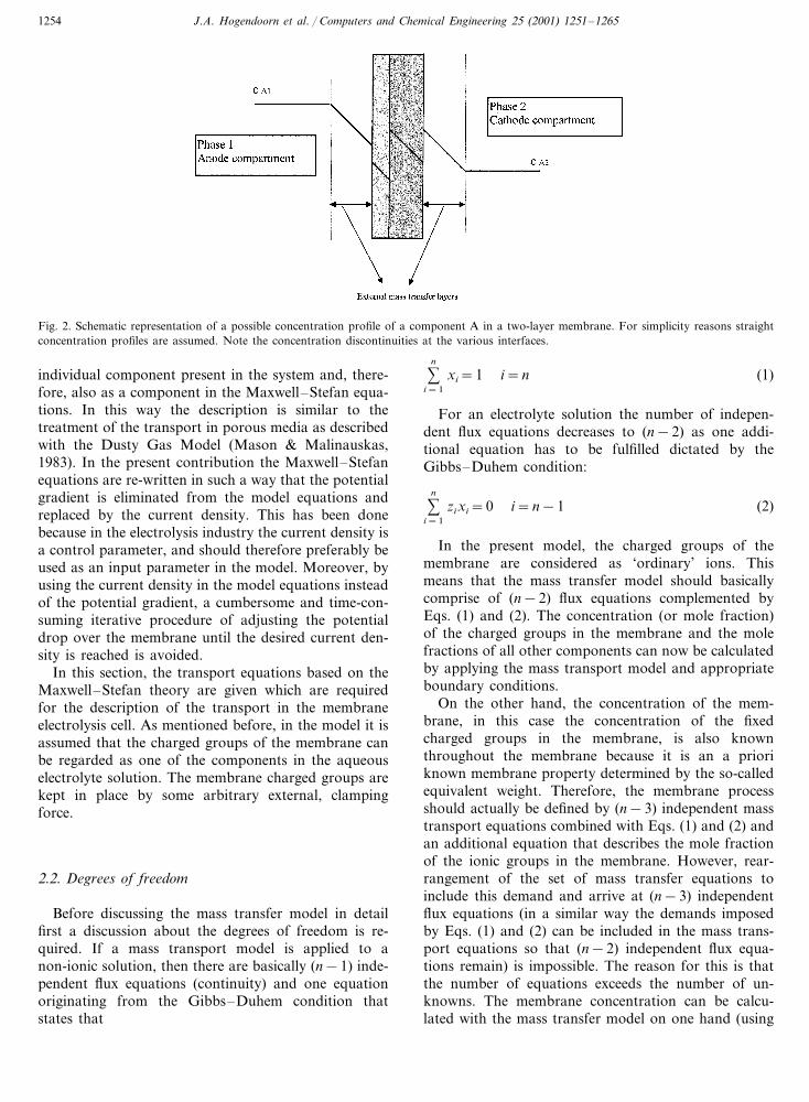
contacted with an electrolyte solution (often referred toas Donnan exclusion). The membrane rejects equallycharged ions (co-ions), while oppositely charged ions(counter-ions) are preferentially absorbed. The variouslayers in the membrane will differ with respect to thesorption properties of the ions and water, resulting inconcentration discontinuities at the various phase tran-sitions (see for example Fig. 2). Also the transportproperties of the ions in the different membrane layerswill vary. Both aspects, the sorption of the ions at thevarious interfaces and the transport of the ions in themembrane layers, have to be incorporated in a masstransfer model in order to obtain a reliable simulationmodel. Furthermore, the mass transfer model itselfshould, of course, represent the actual mass transferphenomena occurring in the membrane in a realisticway. The sorption of ions at the various membraneinterfaces is usually described by the Donnan equilibria.However, this is a very simplified representation ofreality. van der Stegen, van der Veen, Weerdenburg,Hogendoorn and Versteeg (1999a) has shown that theequilibria at the liquid–membrane interfaces can bemore accurately be described using a modified Pitzerequilibrium model.

In the present contribution, a mass transfer modelbased on the Maxwelll–Stefan theory will be developedin order to describe the mass transfer through ion-selec-tive layers. For the description of the equilibria at theliquid–membrane interfaces as required in the masstransfer model the modified Pitzer model as previouslydeveloped by van der Stegen et al. (1999a) is used.

2. Application of the Maxwell–Stefan theory to themembrane electrolysis process

2.1. Introduction

In the present model formulation the charged groupsof the ion-selective membranes are considered as an

Fig. 1. Schematic representation of the chloralkali process in a membrane cell.


Fig. 2. Schematic representation of a possible concentration profile of a component A in a two-layer membrane. For simplicity reasons straightconcentration profiles are assumed. Note the concentration discontinuities at the various interfaces.

individual component present in the system and, there-fore, also as a component in the Maxwell–Stefan equa-tions. In this way the description is similar to thetreatment of the transport in porous media as describedwith the Dusty Gas Model (Mason & Malinauskas,1983). In the present contribution the Maxwell–Stefanequations are re-written in such a way that the potentialgradient is eliminated from the model equations andreplaced by the current density. This has been donebecause in the electrolysis industry the current density isa control parameter, and should therefore preferably beused as an input parameter in the model. Moreover, byusing the current density in the model equations insteadof the potential gradient, a cumbersome and time-con-suming iterative procedure of adjusting the potentialdrop over the membrane until the desired current den-sity is reached is avoided.

In this section, the transport equations based on theMaxwell–Stefan theory are given which are requiredfor the description of the transport in the membraneelectrolysis cell. As mentioned before, in the model it isassumed that the charged groups of the membrane canbe regarded as one of the components in the aqueouselectrolyte solution. The membrane charged groups arekept in place by some arbitrary external, clampingforce.

2.2. Degrees of freedom

Before discussing the mass transfer model in detailfirst a discussion about the degrees of freedom is re-quired. If a mass transport model is applied to anon-ionic solution, then there are basically (n−1) inde-pendent flux equations (continuity) and one equationoriginating from the Gibbs–Duhem condition thatstates that

�n

i=1

xi=1 i=n (1)

For an electrolyte solution the number of indepen-dent flux equations decreases to (n−2) as one addi-tional equation has to be fulfilled dictated by theGibbs–Duhem condition:

�n

i=1

zixi=0 i=n−1 (2)

In the present model, the charged groups of themembrane are considered as ‘ordinary’ ions. Thismeans that the mass transfer model should basicallycomprise of (n−2) flux equations complemented byEqs. (1) and (2). The concentration (or mole fraction)of the charged groups in the membrane and the molefractions of all other components can now be calculatedby applying the mass transport model and appropriateboundary conditions.

On the other hand, the concentration of the mem-brane, in this case the concentration of the fixedcharged groups in the membrane, is also knownthroughout the membrane because it is an a prioriknown membrane property determined by the so-calledequivalent weight. Therefore, the membrane processshould actually be defined by (n−3) independent masstransport equations combined with Eqs. (1) and (2) andan additional equation that describes the mole fractionof the ionic groups in the membrane. However, rear-rangement of the set of mass transfer equations toinclude this demand and arrive at (n−3) independentflux equations (in a similar way the demands imposedby Eqs. (1) and (2) can be included in the mass trans-port equations so that (n−2) independent flux equa-tions remain) is impossible. The reason for this is thatthe number of equations exceeds the number of un-knowns. The membrane concentration can be calcu-lated with the mass transfer model on one hand (using


(n−2) independent flux equations combined with Eqs.(1) and (2)), but at the same time it can be regarded asa membrane property and hence the mole fraction canalso be calculated from that (so without any masstransfer model). This makes the problem over-specified.If it is kept in mind that the Maxwell–Stefan theory isin fact a force balance, this over-specification can beexplained, in the mass transport model no clampingforce for the membrane groups is inserted, which isactually required to keep the membrane at its positionduring the transport process. If this force was intro-duced, there would be one extra degree of freedom andthe system would be described mathematically correct.However, it seems not useful to introduce such aclamping force because it would simply be a fittedparameter. Therefore, it was omitted from the model,which results in an over-specified problem from a fun-damental point of view. Based on this complication twocorrectional approaches can be followed.1. Solving (n−2) equations of continuity. The mole

fractions of the other two components follow fromthe summation of the mole fractions (Eq. (1)) andthe condition of electroneutrality (Eq. (2)).

2. Solving the equation of continuity in combinationwith the specified membrane concentration. Thenumber of continuity equations of continuity is inthis case n−3. The mole fractions of the other threecomponents follow from the summation of the molefractions (Eq. (1)), the condition of electroneutrality(Eq. (2)) and from the specified membraneconcentrations.

If the first method is followed, then the molar fluxesof all components turn out to be constant in the steadystate (i.e. the molar fluxes are no function of position inthe mass transfer layer). However, the calculated mem-brane concentration does not exactly coincide with theindependently determined and a priori known mem-brane concentration. On the other hand, if the secondapproach is followed this discrepancy is avoided be-cause this concentration has been imposed. However, inthis case the molar flux of one component is notconstant in the steady state. It is obvious that a choicehas to be made between.1. Demanding that all components have a constant

molar flux in the steady state, which implies that themembrane concentration cannot be specified. Pre-liminary model calculations (the complete model istreated in subsequent sections) have shown that inthis case deviations between the experimental mem-brane concentration and the calculated membraneconcentration up to a few percent can occur.

2. Specifying the membrane concentration. In this casethe molar flux of one component is not constant.Scouting calculations with the model (presented inSection 2.3) have shown that for this case variationsin the molar flux of this component up to 30% canoccur.

For the present study the first approach was selected.A fundamental principle of mass transfer processes isthat the molar fluxes of all components are constant inthe steady state, so that no accumulation in the systemoccurs.

2.3. Deri�ation of the transport equations for the masstransfer in an electrochemical system

The Maxwell–Stefan theory is a steady state forcebalance in which the total sum of the driving forcesacting on a molecule of a certain component are equalto the friction forces acting on the molecule. In multi-component systems all interactions (frictions) between amolecule with other types of molecules present in thesolution are taken into account. For each component iin a mixture a Maxwell–Stefan equation can be formu-lated, which can be represented as (Taylor & Krishna,1993):

ci�T,P�i=RT �n

j=1

cicj

cTÐi, j

(�j−�i)=RT �n

j=1

xiNj−xjNi

Ði, j

(3)

The left hand side of Eq. (3) contains all drivingforces of the mass transfer process, the right hand sidecontains the interactions between a component i withall other components present in the system. The frictionbetween the various components is lumped in the vari-ous Maxwell–Stefan diffusivities, Ði,j, which are a mea-sure of the interaction between component i and j.

In Eq. (3) the electrochemical potential is defined as:

�i=� ichemical+ziF�=� i

0+RT ln(xi�i)+ziF� (4)

For the development of the present model the mainassumptions are.� No convective transport due to pressure differences

over the membrane occurs. However, in practice, asmall pressure difference over the membrane (�0.1bar) is applied in order to assure that the membraneis pressed against the anode. Preliminary estima-tions, however, have shown that the pressure differ-ence causes a negligible contribution to the totaldriving force compared with those of the concentra-tion and potential gradient (Taylor & Krishna,1993).

� The transport process in the membrane is isother-mal. The assumption that the mass transfer processis isothermal, makes it superfluous to implement andsimultaneously solve the energy balance in the masstransport model. This assumption is allowed becauseno reactions, and, therefore, no heat consumption orevolution takes place inside the membrane. More-over, the heat generated due to Ohmic resistance(calculated according to the method described inTaylor & Krishna, 1993) was estimated to be negligi-ble: for typical conditions of the chloralkali electrol-


ysis process the temperature rise in the membranewas less than 0.2 K.As a result of the above assumptions the mass trans-

fer rate is determined by two gradients, a gradient inthe activity (xi�i) and a gradient in the electrical poten-tial. It is possible to combine these gradients into oneoverall gradient of the mole fraction. In this way, thedriving force of the mass transfer process can be ex-pressed as a function of one set of variables, the molefractions of the components present in the mixture.Solving the transport equations for a specified currentdensity results in this case in the calculation of the molefraction profile and the molar fluxes. With these resultsthe electrical potential profile in the membrane can thenbe obtained. The exact derivation of the resulting trans-port equations has been given in Appendix A. The masstransfer process in a mixture consisting of n compo-nents (including the solvent as the (n−1)th and themembrane charged groups as the nth component) canbe described with the following equations (in matrixnotation).� n−2 Independent Maxwell–Stefan equations for

components 1 to n−2:

(N)= [A ](�x)− [� ]x (5)

in which N is the matrix with the (n−2) fluxes withrespect to the (in time and space stationary) mem-brane (see Appendix A).

� Two supplementary equations for component n−1and n :

�n

i=1

xi=1 i=n (1)

�n

i=1

zixi=0 i=n−1 (2)

For steady state operation, the equation of continuityholds:�dNi

dz�

=0 i=1, 2, …, n (6)

and, therefore, the molar fluxes are not functions ofposition in the membrane.

The set of Eqs. (1), (2), (5) and (6) are second orderdifferential equations. So, for each component twoboundary conditions are required in order to solve theset of equations uniquely.

2.3.1. Boundary conditionsIt is assumed that at the phase transition between

liquid and membrane at both the anolyte and catholyteside locally equilibrium holds (see Fig. 2, note that thisdoes not implicate that no mass transfer resistance canbe present in the liquid (or membrane)). For an ion-se-lective material these equilibria are often described us-

ing Donnan-equilibrium expressions. In a previouspaper, van der Stegen et al. (1999a) has shown thatthese equilibria can more extensively and accurately bedescribed by a modified Pitzer equilibrium model. Thismodel has been used to predict the composition justinside the membrane at x=0 and x=L for a givencomposition just outside the membrane (i.e. catholyteand anolyte side, see Fig. 2 for a schematic representa-tion). This way the boundary conditions for the masstransfer model could be determined.

2.3.2. Numerical techniqueIn the present study, a numerical technique was used

which enables the calculation of the non-steady stateversion of Eq. (6). The resulting set of partial differen-tial equations was solved with the help of a finitedifference technique as proposed by Baker and Oli-phant (Taylor, Hoefsloot & Kuipers, 1995). The mainreason for solving the unsteady state version of Eq. (6)in combination with Eqs. (1), (2) and (5) is that thenumerical solution method is more stable and lesssensitive to the initial guesses. For this unsteady statecalculation procedure initial concentration profiles arerequired, which were arbitrarily chosen as straight con-centration profiles in each mass transfer layer inside themembrane. The calculation procedure was continueduntil the concentration profiles became time-indepen-dent, which meant that a steady state situation wasobtained.

It is emphasized that in the presently derived form ofthe Maxwell–Stefan equations, the current density is aninput parameter, and not a parameter which can onlybe determined after the complete mass transfer problemis solved. This means that with the present formulationa cumbersome, time consuming, iterative procedure isavoided.

2.4. Computer model

Based on the theory presented, a mathematical modelhas been developed and solved numerically. As alreadymentioned in the previous section an implicit discretiza-tion technique according to the scheme of Baker andOliphant was used for the discretization of the partialdifferential equations (see Taylor et al., 1995).

The computer model contains the following elements.1. The number of components can be chosen freely.2. The number of mass transfer layers can be chosen

freely including external mass transfer resistances.For each mass transfer layer, the model needs aspecific set of data with the physical and thermody-namic properties and the material properties (for themembrane phases) of that layer. The required datacan be inserted in the computer model. The requiredphysical parameters can be implemented as a func-tion of composition, temperature and pressure.


3. The computer model includes the modified Pitzermodel for the determination of the activity coeffi-cients in the membrane and the equilibria at thevarious interfaces (see van der Stegen et al., 1999a).

For any arbitrary initial profile, the computer modelcalculates the steady state of the mass transfer processand returns the mole fraction profiles and molar fluxesof the components present in the system as a functionof position. Further, also the electrical potential profileis calculated using Eq. (A.13) (see Appendix A).

2.5. Verification of the algorithm of the computermodel

The algorithm of the computer model was extensivelyverified; i.e. the results of the model were comparedwith the analytical results for various asymptotic situa-tions. In another paper (van der Stegen van der Veen,Weerdenburg, Hogendoorn & Versteeg, 1999b), themodel results are fitted to experimental results of achloralkali electrolysis process to obtain a set ofMaxwell–Stefan diffusivities for this process and there-with be able to predict the performance of the processat various conditions.

Firstly, for both a single layer and a multi-layermembrane (with arbitrarily chosen properties), the con-dition of the continuity of the fluxes was verified. Thefluxes were constant with less than 10−4% difference atthe various positions in the membrane (even at theinterfaces where due to the liquid–membrane or mem-brane–membrane transition a discontinuity in the molefractions occurs, these equilibria are described by themodified Pitzer model as developed by van der Stegenet al. (1999a)). Secondly, for a one layer membrane themodel output (mole fraction profile and potentialprofile) was substituted in the original Maxwell–Stefanequations (relation 1), which yielded a good agreement.Thirdly, a one layer membrane was fictively subdividedin three different separate layers, all having identicalproperties. The model results for the one layer model

were identical to that of the three layer model.Fourthly, for a very diluted 1:1 electrolyte solutionwithout the presence of a membrane or potential differ-ence, the model results were compared with Fick’s law(which is valid for these conditions), which also yieldedexcellent agreement. Fifthly, for a very diluted elec-trolyte solution containing no membrane and 1 type ofpositive ions and two types of negative ions (e.g. aNaOH/NaCl aqueous mixture), the model output wascompared with the predictions of the Nernst–Planckmodel for a current density of CD=0 A m−2 andCD=1 A m−2. For these conditions, the Nernst–Planck model yields an approximate solution for theMaxwell–Stefan equations. Also this comparisonshowed a good agreement. Furthermore, severalasymptotic situations have been simulated, to see if themodel behaves according to the expectations. For ex-ample, in one of the simulations carried out a threelayer membrane was chosen, in which the diffusivitiesin the second layer were chosen very large. Indeed, themodel results indicated that the mole fraction andpotential profile were nearly flat (i.e. constant) in thesecond layer.

From the test results, it was concluded that theoutcome of the computer model satisfies the originalmodel equations. Thus it can be used reliably to simu-late the mass transfer process according to theMaxwell–Stefan theory in a membrane used in thechloralkali electrolysis process.

3. Model simulations

In this section, the results of the model simulationswill be presented which demonstrate the influence ofprocess parameters on the performance of the chloral-kali electrolysis process. This influence on the perfor-mance is simulated for a relatively simple configurationconsisting of a single-layer cation-selective sulfonicmembrane for conditions as encountered in the chloral-kali electrolysis process. The present study gives somenumerical examples to show the capabilities of themodel without extensive comparison or fitting to exper-imental chloralkali electrolysis data, this is done inanother study (van der Stegen et al., 1999b). Becauseno complete set of Maxwell–Stefan diffusivities for thevarious components is available for these ion-selectivesulfonic membranes, and because the present study isnot aimed at an extensive comparison with experimen-tal data a reduced set of Maxwell–Stefan diffusivitieswas used in the simulations. In Table 1 all Maxwell–Stefan diffusivities as encountered in the chloralkaliindustry are summarized. To determine the set of rele-vant Maxwell–Stefan diffusivities, initially, all thesediffusivities were given an equal value of 1.10−10 m2

s−1. This value was derived from the approximate

Table 1The Maxwell–Stefan diffusivities and the selection which has beenincorporated in the model calculations

Incorporated in the calculationsDiffusivity

ÐCl−w YesÐOH−w YesÐNa+w Yes

YesÐm,w

ÐCl−OH− NoNoÐCl−Na+

NoÐCl−m

ÐOH−Na+ NoÐOH−m No

YesÐNa+m


Table 2Base case conditions and calculated performance of the sulfonicmembrane for these conditionsa

Membrane and process conditions

NaCl in anolyte 180 g dm−3

NaOH in catholyte 23 wt.%5pH anolyte

61.8×10−6 mThickness sulfonic membrane1100 g mol−1EWmembrane

Current density (CD) 2000 A m−2

CatholyteAnolyteCalculated mole fractions (−)0.055Cl− 2.03×10−5

Na+ 0.055 0.1060.1060OH−

0.89H2O 0.79

Calculated data1.98×10−2Flux Na+ (mol m−2 s−1)4.40×10−5Flux Cl− (mol m−2 s−1)

Flux OH− (mol m−2 s−1) −9.36×10−5

8.45×10−2Flux H2O (mol m−2 s−1)4.08 molWater transport number

F−1

95.7%Current efficiency (CE)0.149 VPotential drop

a A positive flux resembles a flux from the anode to the cathodeside.

The sulfonic membrane chosen has the same proper-ties as the sulfonic layer of the Nafion DuPont mem-brane with an equivalent weight of 1.1 kg mol−1. In aprevious paper (van der Stegen et al., 1999a) developeda modified Pitzer equilibrium model to describe theequilibria between a liquid and an ion-selective mem-brane. In the present mass transport model equilibriumis assumed at the membrane– liquid interfaces. Thismeans that the modified Pitzer model can be used topredict the concentrations of various species just insidethe membrane for a given composition of the liquid justoutside the membrane. In the mass transfer model it isfurther assumed that the mass transfer resistance fromthe bulk towards the membrane is negligible, so thecomposition at the liquid side of the membrane– liquidinterfaces is equal to the anode and cathode composi-tion, respectively. This means that the overall resistanceagainst mass transfer is located in the membrane itself.

The influence of the thickness of the membrane (30–75 �m), the anolyte concentration (150–220 g l−1) thecurrent density (500–2500 A m−2) and the pH in theanolyte compartment (Eqs. (1)– (6)), respectively, werestudied by varying these parameters around a base case.The conditions of the base case and the correspondingsimulated performance are given in Table 2. As can beseen in Table 2 the current efficiency is much higherthan encountered in industrial chloralkali operation(95.7%). This is due to the fact that all diffusivities werechosen equal and the value of the diffusivities was moreor less chosen arbitrarily at a value of 1.10−10 m2 s−1.This means that the absolute values of the performanceparameters (e.g. potential drop and current efficiencies)are not directly comparable to values obtained duringindustrial operation, but the model can still be used topredict several trends in the aforementionedparameters.

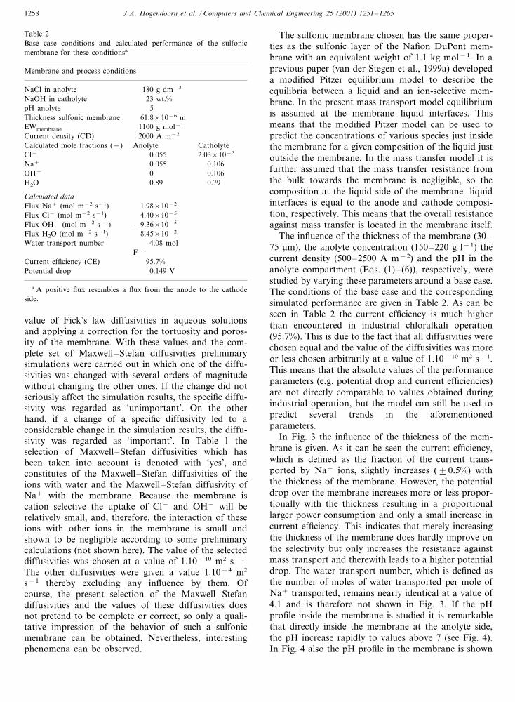
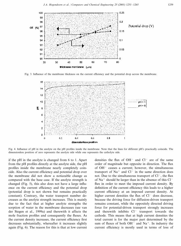
In Fig. 3 the influence of the thickness of the mem-brane is given. As it can be seen the current efficiency,which is defined as the fraction of the current trans-ported by Na+ ions, slightly increases (�0.5%) withthe thickness of the membrane. However, the potentialdrop over the membrane increases more or less propor-tionally with the thickness resulting in a proportionallarger power consumption and only a small increase incurrent efficiency. This indicates that merely increasingthe thickness of the membrane does hardly improve onthe selectivity but only increases the resistance againstmass transport and therewith leads to a higher potentialdrop. The water transport number, which is defined asthe number of moles of water transported per mole ofNa+ transported, remains nearly identical at a value of4.1 and is therefore not shown in Fig. 3. If the pHprofile inside the membrane is studied it is remarkablethat directly inside the membrane at the anolyte side,the pH increase rapidly to values above 7 (see Fig. 4).In Fig. 4 also the pH profile in the membrane is shown

value of Fick’s law diffusivities in aqueous solutionsand applying a correction for the tortuosity and poros-ity of the membrane. With these values and the com-plete set of Maxwell–Stefan diffusivities preliminarysimulations were carried out in which one of the diffu-sivities was changed with several orders of magnitudewithout changing the other ones. If the change did notseriously affect the simulation results, the specific diffu-sivity was regarded as ‘unimportant’. On the otherhand, if a change of a specific diffusivity led to aconsiderable change in the simulation results, the diffu-sivity was regarded as ‘important’. In Table 1 theselection of Maxwell–Stefan diffusivities which hasbeen taken into account is denoted with ‘yes’, andconstitutes of the Maxwell–Stefan diffusivities of theions with water and the Maxwell–Stefan diffusivity ofNa+ with the membrane. Because the membrane iscation selective the uptake of Cl− and OH− will berelatively small, and, therefore, the interaction of theseions with other ions in the membrane is small andshown to be negligible according to some preliminarycalculations (not shown here). The value of the selecteddiffusivities was chosen at a value of 1.10−10 m2 s−1.The other diffusivities were given a value 1.10−4 m2

s−1 thereby excluding any influence by them. Ofcourse, the present selection of the Maxwell–Stefandiffusivities and the values of these diffusivities doesnot pretend to be complete or correct, so only a quali-tative impression of the behavior of such a sulfonicmembrane can be obtained. Nevertheless, interestingphenomena can be observed.


Fig. 3. Influence of the membrane thickness on the current efficiency and the potential drop across the membrane.

Fig. 4. Influence of pH in the anolyte on the pH profiles inside the membrane. Note that the lines for different pH’s practically coincide. Thedimensionless position of zero represents the anolyte side while one represents the catholyte side.

if the pH in the anolyte is changed from 6 to 1. Apartfrom the pH profiles directly at the anolyte side, the pHprofiles inside the membrane nearly completely coin-cide. Also the current efficiency and potential drop overthe membrane did not show a noticeable change ascompared with the base case. If the anolyte strength ischanged (Fig. 5), this also does not have a large influ-ence on the current efficiency and the potential drop(potential drop is not shown but remains practicallyconstant). Contrary, the water transport number de-creases as the anolyte strength increases. This is mainlydue to the fact that at higher anolyte strengths thesorption of water in the membrane decreases (see vander Stegen et al., 1999a) and therewith it affects themole fraction profiles and consequently the fluxes. Asthe current density increases, the current efficiency firstdecreases substantially, whereafter it increases slightlyagain (Fig. 6). The reason for this is that at low current

densities the flux of OH− and Cl− are of the sameorder of magnitude but opposite in direction. The fluxof OH− causes a current; however, the simultaneoustransport of Na+ and Cl− in the same direction doesnot. Due to the simultaneous transport of Cl−, the fluxof Na+ should be larger than in the absence of this Cl−

flux in order to meet the imposed current density. Bydefinition of the current efficiency this leads to a highercurrent efficiency at an imposed current density. Athigher current densities the flux of Cl− does decrease,because the driving force for diffusion-driven transportremains constant, while the oppositely directed drivingforce for potential-driven transport strongly increasesand therewith inhibits Cl− transport towards thecathode. This means that at high current densities thetotal current is for the major part determined by thesum of fluxes of both OH− and Na+. In industry thecurrent efficiency is mostly used in terms of loss of


Fig. 5. Influence of the anolyte strength on the current efficiency (%) and the water transport number (mol F−1).

Fig. 6. Influence of the current density on the current efficiency and the potential drop across the membrane.

current due to the counter transport of OH−. However,this example illustrates that at low current densities thisrule-of-thumb definition of the current efficiency cangive misleading results, although the current efficienciescalculated for low current densities seem attractivelyhigh, this is due to the definition of the current densityand is at the expense of contamination of the catholytewith Cl−. As it can be expected the potential dropacross the membrane is proportionally dependent onthe current density (Fig. 6).

4. Conclusions

A model has been developed which describes themass transfer in ion-selective membranes as used in the

chloralkali electrolysis process. The mass transfermodel is based on the Maxwell–Stefan theory, in whichthe membrane charged groups were considered as oneof the components in the aqueous mixture. TheMaxwell–Stefan equations were re-written in such away that the current density can be used as an inputparameter in the model, which circumvents an extensivenumerical iterative process in the numerical solution ofthe equations. Due to the fact that the Maxwell–Stefantheory is in fact a force balance, and the clamping forceneeded to keep the membrane charged groups in itsplace is not taken into account, the model is basicallyover-specified, the mole fraction of the membrane canbe calculated by using the equivalent weight (EW) ofthe membrane or by using the equations of continuity.The model itself is able to predict the mole fraction of


the membrane charged groups using the equations ofcontinuity, but this fraction can also be calculated apriori because it is a membrane property determined bythe equivalent weight. It was decided not to use theequation that gives the membrane mole fraction basedon the equivalent weight, but use the equation ofcontinuity instead. This yielded only a few percentdifference between the two differently calculated mem-brane mole fractions. The results of the computermodel were verified in several ways, which showed thatthe computer model gives reliable results. Several ex-ploratory simulations have been carried out for a sul-fonic layer membrane and the conditions asencountered in the chloralkali electrolysis process. Inthe calculations a selection of the Maxwell–Stefan dif-fusivities was used, the selection being based on asensitivity analysis. Because in literature no accurateMaxwell–Stefan diffusivities are available for ion-selec-tive membranes (or other systems) the selected diffusiv-ities were chosen equal in these exploratorycalculations. Therefore, the absolute values of the vari-ous performance parameters are incorrect as comparedwith industrial operation (e.g. current efficiency andpotential drop), but the model can be used to predicttrends in these parameters with a change in operatingconditions. It was shown that the thickness of themembrane hardly increases the current efficiency, how-ever, the required potential drop proportionally in-creases with it. The pH rapidly increases to values �12just inside the membrane at the anolyte side. Moreover,for different values of the pH in the anolyte, the pHprofiles inside the membrane nearly coincide. A changein the anolyte strength does not seem to have a signifi-cant effect on the performance of the membrane. A lowcurrent density shows a high current efficiency, but thisis due to an artifact, because it is not caused by adesired low OH− counter flux but by the undesiredtransport of Cl− towards the catholyte. It is clear thatthe model needs a reliable input for the Maxwell–Ste-fan diffusivities before it can be used to reliably simu-late the performance of an industrially used membraneand applications in development and design. In anotherpaper, these diffusivities have been be determined forthe industrially used Nafion membrane of DuPont (vander Stegen et al., 1999b).

Appendix A. Development of the mass transfer model

A.1. Introduction

In this appendix the complete mass transfer modelfor an electrochemical system will be developed. Thefundamentals of this model are constituted by the masstransport equations, which describe the mass transfer inan electrochemical system. These equations are derived

in subsection A.2. For the complete description of themass transfer in an electrochemical system a number ofadditional equations should be added to the mass trans-port equations. In subsection equation, A1.3 the com-plete model is given which includes all relevantequations.

A.2. Deri�ation of the mass transport equations

Starting point for the derivation of the set of masstransport equations is the Maxwell–Stefan equation forcomponent i2:

ci�T,P�i=RT �n

j=1

cicj

cTÐi, j

(�j−�i)=RT �n

j=1

xiNj−xjNi

Ði, j

(A.1)

The driving force for the mass transport is the elec-trochemical potential gradient ��i, in which the electro-chemical potential �i is defined as follows:

�i=� ichemical+ziF�=� i

o+RT ln(xi�i)+ziF� (A.2)

The main assumption in the above formulation of theMaxwell–Stefan equation and the equation for theelectrochemical potential of component i is that pres-sure differences and/or other external forces do notaffect the mass transfer process. Besides, it is assumedthat the transport process takes place isothermally.

It is preferable to express the driving force of themass transfer process as a function of one set ofvariables, namely the mole fractions of the componentspresent in the liquid mixture. The derivation of thetransport equations can be split into three parts:1. Derivation of an expression of the electrical poten-

tial gradient as a function of the gradient in theactivity.

2. Derivation of an expression of the gradient in theactivity as a function of the gradient in the molefractions.

3. Rearrangement of the set of Maxwell–Stefanequations.

A.2.1. Deri�ation of an expression of the electricalpotential gradient as a function of the gradient in theacti�ity (see also Newman, 1963)

The Maxwell–Stefan equation for component i canbe rewritten as3:

2 In the following ��k should be read as �T,P�k.3 �n

j=1 Ki, j(�j−�i)=�nj=1 Ki, j(�j−�i)−�n�n

j=1 Ki, j+�n �nj=1 Ki, j

=�nj=1j� i

Ki, j�j+Ki,i�i−�nj=1 Ki, j�i

−�n �nj=1j� i

Ki, j−�nKi,i+�n�nj=1Ki, j

=�nj=1j� i

Ki, j(�j−�n)

+ (Ki,i−�nj=1 Ki, j)(�i−�n)

=�nj=1 Mi, j(�j−�n).


ci��i=RT �n

j=1

cicj

cTÐi, j

(�j−�i)= �n

j=1

Ki, j(�j−�i)

= �n

j=1

Mi, j(�j−�n) (A.3)

with:

Mi, j=Ki, j i� j=1, 2, …, n (A.3a)

Mi,i=Ki,i− �n

k=1

Ki,k i=1, 2, …, n (A.3b)

Ki, j=RTxixjcT

Ði, j

(A.3c)

The mass transport in a mixture of n components canbe described fundamentally with n Maxwell–Stefanequations. However, due to the Gibbs–Duhem rela-tionship only n−1 Maxwell–Stefan equations are inde-pendent. With this restriction, the preceding Eq. (A.3c)can be rewritten as:

�j−�n= − �n−1

k=1

Lj,kn ck��k (A.4)

with:

[Ln]= − [Mn]−1 (A.4a)

[Mn] is obtained from [M ] in which the nth row and thenth column has been removed4.

The current density I can be obtained from thecomponent velocities5:

I=F �n

i=1

zici�i=F �n−1

i=1

zici�i+Fzncn�n

=F �n−1

i=1

zici�i−F�n �n−1

i=1

zici=F �n−1

i=1

zici(�i−�n)

= −F �n−1

i=1

zici �n−1

k=1

Li,kn ck��k

= −F �n−1

i=1

ci��i �n−1

k=1

Lk,in ckzk (A.5)

Definition of � and t in

If no concentration gradients are present in the liquidphase, then the expression for the electrochemical po-tential gradient reduces to:

��i=ziF�� (A.6)

Substitution of Eq. (A.6) into Eq. (A.5) results in thefollowing relation for I :

I= −F2�� n−1

i=1

zici �n−1

k=1

Li,kn zkck= −�� (A.7)

with:

�=cT2 F2 �

n−1

i=1

�n−1

j=1

zizjxixjLi, jn (A.8)

In other words, if no concentration-driven masstransfer occurs, then the relationship between the cur-rent density and the electrical potential gradient followsOhm’s law (� is the conductivity of the solution, 1/� isa kind of electrical resistance).

The contribution of each component to the currentdensity I can be expressed with the help of a transfer-ence number for each component (except the nth). Thetransference number t i

n is defined as follows:

t inI=−t i

n��=ciziF(�i−�n)� t in

=zixicT

2 F2

��

n−1

k=1

Li,kn zkxk (A.9)

N.B.:

�n−1

i=1

t in=1

Eq. (A.8) can also be written as:

�n−1

k=1

Li,kn zkxk=

t in�

zixicT2 F2 (A.10)

Introduction of � and t in in the relation Eq. (A.9)

If concentration gradients are present in the liquidphase (which is the case with membrane processes),then Eq. (A.5) changes after combination with Eq.(A.10) to:

I= −F �n−1

i=1

ci��i �n−1

k=1

Lk,in ckzk= −

�

F�

n−1

i=1

t in

zi

��i (A.11)

Substitution of Eq. (A.2) in Eq. (A.11) results into:

I= −�

F�

n−1

i=1

t in

zi

{RT�(ln(xi�i))+ziF��}

= −��−RT�

F�

n−1

i=1

t in

zi

�(ln(xi�i)) (A.12)

from which the following expression for the electricalpotential gradient is obtained:

��= −I�

−1F

�n−1

i=1

t in

zi

�� ichemical

= −I�

−RTF

�n−1

i=1

t in

zi

�(ln(xi�i)) (A.13)

The first part of the right hand side of Eq. (A.13)gives the Ohmic contribution to the electrical potential,the second part gives the diffusion potential, which is acorrection of the electrical potential gradient due to thepresence of concentration differences in the solution.

4 Note that [M ], [Mn] and [Ln] are symmetrical.5 With the derivation of Eq. (A.5) the condition of electroneutrality

has been applied, which can be formulated as follows �ni=1 zixi=

cT�ni=1 zixi=�n

i=1 zici=0.


A.2.2. Deri�ation of an expression of the gradient inthe acti�ity as a function of the gradient in the molefractions

Rearrangement of the set of Maxwell–Stefanequations.

According to Taylor and Krishna (1993) the follow-ing expression can be derived:

di= �n−1

j=1

�i, j�xj−xiziFIRT�

= �n

j=1

xiNj−xjNi

cTÐi, j

(A.14)

As pointed out by Taylor and Krishna (1993), themolar flux Ni needs to be defined with respect to acertain reference frame. For this case, the velocity ofthe nth component will be chosen as the referenceframe in order to obtain the diffusive flux of the othercomponents. For the diffusive flux (Ji

n), which is theflux of component i with respect to the velocity ofcomponent n, the following relation can be derived:

Jin=Ni−ci�n (A.15)

The diffusive flux Jnn is equal to zero with this defini-

tion (Taylor & Krishna, 1993).Eq. (A.14) can now be rearranged to (Taylor &

Krishna, 1993):

di= �n−1

j=1

Bi, jn J j

n (A.16)

with:

Bi,in = −

1cT

�n

k=1 i�k

xk

Ði,k

i=1, 2, …, n−1 (A.16a)

Bi, jn =

xi

cTÐi, j

i� j=1, 2, …, n−1 (A.16b)

The set of n−1 Maxwell–Stefan equations for thedescription of the mass transfer in an n-componentmixture can be represented in matrix notation asfollows:

(d)= [�](�x)− (Z)= [Bn](Jn) (A.17)

with:

Zi=xiziFIRT�

i=1, 2, …, n−1 (A.17a)

The gradient in the mole fraction follows from Eq.(A.17):

[�](�x)= [Bn](Jn)+ (Z) (A.18)

However, the set of (n−1) equations defined by Eq.(A.18) contains one dependent equation due to thecondition of electroneutrality. It is possible to eliminatethe dependent equation by substituting the followingrelations into Eq. (A.18):

I=F �n

i=1

ziNi=F �n

i=1

zi J in (A.19)

and:

�n

i=1

�xi=0 (A.20a)

�n

i=1

zi�xi=0 (A.20b)

Rearrangement of Eq. (A.18) with the help of Eqs.(A.19), (A.20a) and (A.20b) yields:

[��](�x)= [Bn* ](Jn)+ (Z*)I (A.21)

with:

�i, j* =�i, j−�i,n−1

zj−zn

zn−1−zn

i=1…n−2;

j=1 ,…, n−2 (A.22a)

Bi, jn *=Bi, j

n −Bi,n−1n zj

zn−1

i=1…n−2;

j=1, …, n−2 (A.22b)

Zi*=�xiziF

RT�+

Bi,n−1n

Fzn−1

�i=1, …, n−2 (A.22c)

Eq. (A.21) can be reworked to:

(Jn)= [A ](�x)− (�)I (A.22)

with:

[A ]= [Bn* ]−1[�* ] (A.22a�)

(�)= [Bn* ]−1(Z*) (A.22b�)

This equation can be further rewritten as:

(Jn)= [A ](�x)− [� ]x (A.23)

with:

[� ]= [Bn* ]−1[Zc]

in which:

Zi, jc =0 i� j=1, 2, …, n−2 (A.24.a)

Zi,ic =

� ziFRT�

+1

FcTÐi,n−1zn−1

�I i=1, 2, …, n−2

(A.24.b)

Relationship (Eq. (A.23)) defines a set of n−2 inde-pendent equations, which can be solved with the help ofto following supplementary equations:

�n

i=1

zixi=0 (condition of electroneutrality)

�n

i=1

xi=1 (A.25)

Eq. (A.23) is the basic equation for the description ofthe mass transport in a electrochemical system. Thisequation can be further adjusted for the membraneelectrolysis process. The membrane in these processes isoften modeled as a component, in which the membrane


concentration is chosen equivalent to the concentrationof the fixed charged groups in the membrane and theionic charge of the membrane (zmembrane) equivalent tothe charge of the charged groups in the membrane. Inmembrane processes the reference velocity with theapplication of the Maxwell–Stefan theory is often thevelocity of the membrane, which is (mostly) 0 m s−1. Ifthe membrane is the nth component Eq. (A.15) can bewritten as:

�n=−1cm

Jmn =0 (A.26)

If the membrane is the nth component in the system,then the molar flux of component i (for i=1, …, n−2)follows from:

Ni=Jin−ci�n=Ji

n−ci

cm

Jin

=Jin−

xi

xmembrane

Jmembranen =Ji

n (A.27)

in which Jin follows from Eq. (A.23). If component

(n−1) is ionic, the flux of this component can be easilycalculated using Eq. (A.19). Otherwise, for component(n−1) it is also possible to calculate the flux by substi-tuting the resulting calculated mole fraction profile inEq. (A.23). With the known mole fraction profile, thepotential profile can now be calculated using Eq.(A.13).

A.3. Final model equations

In conclusion this gives for the present system.� n−2 Independent Maxwell–Stefan equations for

components 1–n−2:

(N)= [A ](�x)− [� ]x (A.28)

in which N is the matrix with the (n−2) fluxes withrespect to the (in time and space stationary)membrane.

� Two supplementary equations for component n−1and n :

�n

i=1

zixi=0 i=n−1 (A.29)

�n

i=1

xi=1 i=n (A.30)

in which matrix A contains diffusivities, thermody-namic non-idealities and transference numbers:

[A ]= [Bn* ]−1[�* ] (A.31)

The matrix [A ] can be divided into two parts:� One matrix with diffusivities [Bn*].� One matrix with thermodynamic non-idealities and

transference numbers [�*]; and matrix � with diffu-sivities and the current density:

[� ]= [Bn* ]−1[Zc] (A.32)

The different matrices are defined as.� Matrix with diffusivities [Bn*]:

Bi, jn *=Bi, j

n −Bi,n−1n zj

zn−1

i=1, …, n−2 (A.33)

with:

Bi,in = −

1cT

�n

k=1k� i

xk

Ði,k

(A.33a)

Bi, jn =

xi

cTÐi, j

i� j (A.33b)

� Matrix with thermodynamic non-idealities and trans-ference numbers [�]:

�ij*=�i, j−�i,n−1

zj−zn

zn−1−zn

i=1, …, n−2

j=1, …, n−2 (A.34)

with:

�i, j=�i, j−xizi �n−1

k=1

�k, j

tkn

zkxk

(A.34a)

�i, j=�i, j+xi

� ln �i

�xj

�T,P,xk,k� j=1…n−1

(A.34b)

t jn=

zjxjcT2 F2

��

n−1

k=1

Lj,kn zkxk (A.34c)

�=cT2 F2 �

n−1

i=1

�n−1

j=1

zizjxixjLi, jn (A.34d)

[Ln]= − [Mn]−1 (A.34e)

[Mn] follows from [M ] in which the nth row andcolumn have been removed:

Mi, j=Ki, j i� j=1, 2, …, n (A.34f)

Mi,i=Ki,i− �n

k=1

Ki,k i=1, 2, …, n (A.34g)

Ki, j=RTxixjcT

Ði, j

(A.34h)

� Matrix with diffusivities and current density Zc:

Zi, jc =0 i� j=1, 2, …, n−2 (A.35a)

Zi,ic =

� ziFRT�

+1

FcTÐi,n−1zn−1

�I i=1, 2, …, n−2

(A.35b)


References

Mason, E. A., & Malinauskas, A. P. (1983). Gas Transport in PorousMedia : The Dusty Gas Model, Chemical Engineering Monographs,vol. 17. Amsterdam: Elsevier.

Newman, J. S. (1963). Electrochemical Systems. Englewoods Cliffs,NJ: Prentice-Hall.

van der Stegen, J. H. G., van der Veen, A. J., Weerdenburg, H.,Hogendoorn, J. A., & Versteeg, G. F. (1999a). Application of thePitzer model for the estimation of activity coefficients of elec-trolytes in ion selective membranes. Fluid Phase Equilibria, 157,

181–196.van der Stegen, J. H. G., van der Veen, A. J., Weerdenburg, H.,

Hogendoorn, J. A., & Versteeg, G. F. (1999b). Application of theMaxwell–Stefan theory to the transport in ion-selective mem-branes used in the chloralkali electrolysis process. Chemical Engi-neering Science, 54, 2501–2511.

Taylor, R., & Krishna, R. (1993). Multicomponent Mass Transfer.New York: Wiley.

Taylor, R., Hoefsloot, H. C. J., & Kuipers, J. A. M. (1995). Readerof the course. In Numerical Method for Chemical Engineers. TheNetherlands: Enschede.

.

Documents

University of Groningen Application of the Maxwell–Stefan