Analysis of Maxwell-Stefan systems for heat conducting uid

ASC Report No. 09/2020

Analysis of Maxwell-Stefan systems for heatconducting fluid mixtures

C. Helmer and A. Jungel

Institute for Analysis and Scientific Computing

Vienna University of Technology — TU Wien

www.asc.tuwien.ac.at ISBN 978-3-902627-00-1

Most recent ASC Reports

08/2020 L. Mascotto, J.M. Melenk, I. Perugia, A. RiederFEM-BEM mortar coupling for the Helmholtz problem in three dimensions

07/2020 R. Becker, M. Innerberger, and D. PraetoriusOptimal convergence rates for goal-oriented FEM with quadratic goal functional

06/2020 A. Rieder, F.-J. Sayas, J.M. MelenkRunge-Kutta approximation for C0-semigroups in the graph norm with applica-tions to time domain boundary integral equations

05/2020 A. Arnold, C. Schmeiser, and B. SignorelloPropagator norm and sharp decay estimates for Fokker-Planck equations withlinear drift

04/2020 G. Gantner, A. Haberl, D. Praetorius, and S. SchimankoRate optimality of adaptive finite element methods with respect to the overallcomputational costs

03/2020 M. Faustmann, J.M. Melenk, M. ParviziOn the stability of Scott-Zhang type operators and application to multilevelpreconditioning in fractional diffusion

02/2020 M. Bulicek, A. Jungel, M. Pokorny, and N. ZamponiExistence analysis of a stationary compressible fluid model for heat-conductingand chemically reacting mixtures

01/2020 M. Braukhoff and A. JungelEntropy-dissipating finite-difference schemes for nonlinear fourth-order parabolicequations

31/2019 W. Auzinger, M. Fallahpour, O. Koch, E.B. WeinmullerImplementation of a pathfollowing strategy with an automatic step-length con-trol: New MATLAB package bvpsuite2.0

30/2019 W. Auzinger, O. Koch, E.B. Weinmuller, S. WurmModular version bvpsuite1.2 of the collocation MATLAB package bvpsuite1.1

Institute for Analysis and Scientific ComputingVienna University of TechnologyWiedner Hauptstraße 8–101040 Wien, Austria

E-Mail: [email protected]

WWW: http://www.asc.tuwien.ac.at

FAX: +43-1-58801-10196

ISBN 978-3-902627-00-1

c© Alle Rechte vorbehalten. Nachdruck nur mit Genehmigung des Autors.

ANALYSIS OF MAXWELL–STEFAN SYSTEMS FOR HEATCONDUCTING FLUID MIXTURES

CHRISTOPH HELMER AND ANSGAR JUNGEL

Abstract. The global-in-time existence of weak solutions to the Maxwell–Stefan–Fourierequations in Fick–Onsager form is proved. The model consists of the mass balance equa-tions for the partial mass densities and and the energy balance equation for the totalenergy. The diffusion and heat fluxes depend linearly on the gradients of the thermo-chemical potentials and the gradient of the temperature and include the Soret and Dufoureffects. The cross-diffusion system exhibits an entropy structure, which originates fromthe consistent thermodynamic modeling. The lack of positive definiteness of the diffusionmatrix is compensated by the fact that the total mass density is constant in time. Theentropy estimate also allows for the proof of the a.e. positivity of the partial mass densitiesand temperature.

1. Introduction

Maxwell–Stefan equations describe the dynamics of multicomponent fluids by account-ing for the gradients of the chemical potentials as driving forces. The global existenceanalysis is usually based on the so-called entropy or formal gradient-flow structure. Up toour knowledge, almost all existence results are concerned with the isothermal setting. Ex-ceptions are the local-in-time existence result of [19] and the coupled Maxwell–Stefan andcompressible Navier–Stokes–Fourier systems analyzed in [17, 24], where no temperaturegradients in the diffusion fluxes (Soret effect) have been taken into account. In this paper,we suggest and analyze for the first time Maxwell–Stefan–Fourier systems in Fick–Onsagerform, including Soret and Dufour effects.

1.1. Model equations. We consider the evolution of the partial mass densities ρi(x, t)and temperature θ(x, t) in a fluid mixture, governed by the equations

∂tρi + div Ji = ri, Ji = −n∑j=1

Mij(ρ, θ)∇qj −Mi(ρ, θ)∇1

θ,(1)

Date: April 13, 2020.2000 Mathematics Subject Classification. 35K51, 35K55, 82B35.Key words and phrases. Fick–Onsager cross-diffusion equations, Maxwell–Stefan systems, fluid mix-

tures, existence of solutions, positivity.The authors have been partially supported by the Austrian Science Fund (FWF), grants P30000,

P33010, F65, and W1245.1

2 C. HELMER AND A. JUNGEL

∂t(ρθ) + div Je = 0, Je = −κ(θ)∇θ −n∑j=1

Mj(ρ, θ)∇qj in Ω, i = 1, . . . , n,(2)

where Ω ⊂ R3 is a bounded domain, ρ = (ρ1, . . . , ρn) is the vector of mass densities, andqi = log(ρi/θ) is the thermo-chemical potential of the ith species. The diffusion fluxes aredenoted by Ji, the reaction rates by ri, the energy flux by Je, and the heat conductivityby κ(θ). The functions Mij are the diffusion coefficients, and the terms Mi∇(1/θ) and∑n

j=1 Mj∇qj describe the Soret and Dufour effect, respectively.We prescribe the boundary and initial conditions

Ji · ν = 0, Je · ν + λ(θ0 − θ) = 0 on ∂Ω, t > 0,(3)

ρi(·, 0) = ρ0i , (ρiθ)(·, 0) = ρ0

i θ0 in Ω, i = 1, . . . , n,(4)

where ν is the exterior unit normal vector to ∂Ω, θ0 > 0 is the constant backgroundtemperature, and λ ≥ 0 is a relaxation parameter. Equations (3) mean that the fluidcannot leave the domain Ω, while heat transfer through the boundary is possible (if λ 6= 0).

In Maxwell–Stefan systems, the driving forces ∇(ρiθ) are usually given by linear combi-nations of the diffusion fluxes [5, Sec. 14]:

(5) ∂tρi + div Ji = ri, ∇(ρiθ) = −n∑j=1

bijρiρj

(Jiρi− Jjρj

), i = 1, . . . , n,

where bij = bji ≥ 0 for i, j = 1, . . . , n. We show in Section 2 that this formulation can bewritten as (1) for a specific choice of Mij and Mi.

We say that the diffusion fluxes in (1) are in Fick–Onsager form. As the heat flux isgiven by Fourier’s law, we call system (1)–(2) the Maxwell–Stefan–Fourier equations inFick–Onsager form. We refer to Section 2 for details of the modeling.

To fulfill mass conservation, the sum of the diffusion fluxes and the sum of the reactionterms should vanish, i.e.

∑ni=1 Ji = 0 and

∑ni=1 ri = 0 (see Section 2). Then, summing (1)

over i = 1, . . . , n, we see that the total mass density ρ(·, t) :=∑n

i=1 ρi(·, t) = ρ0 is constantin time (but generally not in space). Another consequence of the identity

∑ni=1 Ji = 0 is

that the diffusion matrix has a nontrivial kernel, and we assume that

(6)n∑i=1

Mij = 0 for j = 1, . . . , n,n∑i=1

Mi = 0.

Moreover, we suppose that the matrix (Mij) is positive semi-definite in the sense that thereexists cM > 0 such that

(7)n∑i=1

Mij(ρ, θ)zizj ≥ cM |Πz|2 for z ∈ Rn, ρ ∈ Rn, θ ∈ R+,

where Π = I − 1⊗ 1/n is the orthogonal projection on span1⊥. For a discussion of thisassumption, we refer to Section 1.4.

MAXWELL–STEFAN–FOURIER SYSTEMS 3

Notation. We write z for a vector of Rn with components z1, . . . , zn and similarly forother variables. In particular, 1 = (1, . . . , 1) ∈ Rn. Furthermore, we set R+ = [0,∞) andΩT = Ω× (0, T ).

1.2. Mathematical ideas. The mathematical difficulties of system (1)–(2) are the cross-diffusion structure, the lack of coerciveness of the diffusion operator, and the temperatureterms. In particular, it is not trivial to verify the positivity of the temperature. These dif-ficulties are overcome by exploiting the entropy structure of the equations. More precisely,we introduce the mathematical entropy

h(ρ, θ) =n∑i=1

ρi(log ρi − 1)− ρ log θ.

A formal computation (which is made precise for an approximate scheme; see (24)) showsthat

d

dt

∫Ω

h(ρ, θ)dx+ cM

∫Ω

|∇Πq|2dx+

∫Ω

κ(θ)|∇ log θ|2dx+ λ

∫∂Ω

(θ0

θ− 1

)ds(8)

≤n∑i=1

∫Ω

riqidx.

Under suitable conditions on the heat conductivity and the reaction rates, this so-calledentropy inequality provides gradient estimates for Πq, log θ, and θ, but not for the fullvector q. This problem was overcome in [9] for a more general (but stationary) multicom-ponent Navier–Stokes–Fourier system by using tools from mathematical fluid dynamics(effective viscous flux identity and Feireisl’s oscillations defect measure). For our model,the situation is much simpler. Indeed, an elementary computation, detailed in the proofof Lemma 5, shows that

(9)1

n

n∑i=1

∇qi = ∇ log ρ0 −∇ log θ −n∑i=1

ρiρ∇(Πq)i

and consequently ∇qi = ∇(Πq)i +∑n

i=1∇qi/n is bounded in L2. If ρ0 is bounded, thetotal mass density is bounded too, and ρi lies in L∞ for any i = 1, . . . , n. This providesan L2 estimate for ∇ρi = ρi(∇ log θ+∇qi). Together with a bound for the (discrete) timederivative of ρi, we deduce the strong convergence of ρi from the Aubin–Lions compactnesslemma.

The positivity of the temperature is a consequence of the L1 estimate for − log θ comingfrom (8). Still, there remains a difficulty. The estimate for κ(θ)1/2∇ log θ in L2 from (8)is not sufficient to define κ(θ)∇θ in the weak formulation. In the Navier–Stokes–Fourierequations, this difficulty is handled by replacing the local energy balance by the localentropy inequality and the global energy balance [15]. We choose another approach. Theidea is to derive better estimates for the temperature by using θ as a test function in theweak formulation of (2). If κ(θ) ≥ cκθ

2 for some cκ > 0 and Mj/θ is assumed to be


bounded, then a formal computation, which is made precise in Lemma 3, gives

1

2

d

dt

∫Ω

ρ0θ2dx+ cκ

∫Ω

θ2|∇θ|2dx− λ∫∂Ω

(θ0 − θ)θds(10)

=n∑j=1

∫Ω

Mj

θθ∇qj · ∇θdx ≤

cκ2

∫Ω

θ2|∇θ|2dx+ C

n∑j=1

∫Ω

|∇qj|2dx.

Since ∇qj is bounded in L2, this yields uniform bounds for θ2 in L∞(0, T ;L1(Ω)) andL2(0, T ;H1(Ω)). These estimates are sufficient to treat the term κ(θ)∇θ. The delicatepoint is to choose the approximate scheme in such a way that estimates (8) and (10) canbe made rigorous; for details see Section 3.

1.3. State of the art. Before we state our main result, we review the state of the artof Maxwell–Stefan models. The isothermal equations were derived from the multi-speciesBoltzmann equations in the diffusive approximation in [2, 8]. The Fick–Onsager form of theMaxwell–Stefan equations was rigorously derived in Sobolev spaces from the multi-speciesBoltzmann system in [3]. The Maxwell–Stefan equations in the Fick–Onsager form, cou-pled with the momentum balance equation, can be identified as a rigorous second-orderChapman–Enskog approximation of the Euler (–Korteweg) equations for multicomponentfluids; see [18] for the Euler–Korteweg case and [23] for the Euler case. The work [7] isconcerned with the friction limit in the isothermal Euler equations using the hyperbolicformalism developed by Chen, Levermore, and Liu. A formal Chapman–Enskog expansionof the stationary non-isothermal model was presented in [25]. Another non-isothermalMaxwell–Stefan system was derived in [1], but the energy flux is different from the expres-sion in (2).

The existence analysis of (isothermal) Maxwell–Stefan equations started with the paper[16], where the existence of global-in-time weak solutions near the constant equilibrium wasproved. A proof of local-in-time classical solutions to Maxwell–Stefan systems was givenin [4]. In [22], the entropy or formal gradient-flow structure was revealed, which allowedfor the proof of global-in-time weak solutions with general initial data. Maxwell–Stefansystems, coupled to the Poisson equation for the electric potential, were analyzed in [21].

All the mentioned results hold if the barycentric velocity vanishes. For non-vanishingfluid velocities, the Maxwell–Stefan equations need to be coupled to the momentum bal-ance. The Maxwell–Stefan equations were coupled to the incompressible Navier–Stokesequations in [10], and the global existence of weak solutions was shown. A similar resultcan be found in [11], where the incompressibility condition was replaced by an artificialtime derivative of the pressure and the limit of vanishing approximation parameters wasperformed. Coupled Maxwell–Stefan and compressible Navier–Stokes equations were an-alyzed in [6], and the local-in-time existence analysis was performed. A global existenceanalysis for a general isothermal Maxwell–Stefan–Navier–Stokes system was performed in[13]. For the existence analysis of coupled stationary Maxwell–Stefan and compressibleNavier–Stokes–Fourier systems, we refer to [9, 17, 24]. In [9], temperature gradients wereincluded in the partial mass fluxes, but only the stationary model was investigated. The


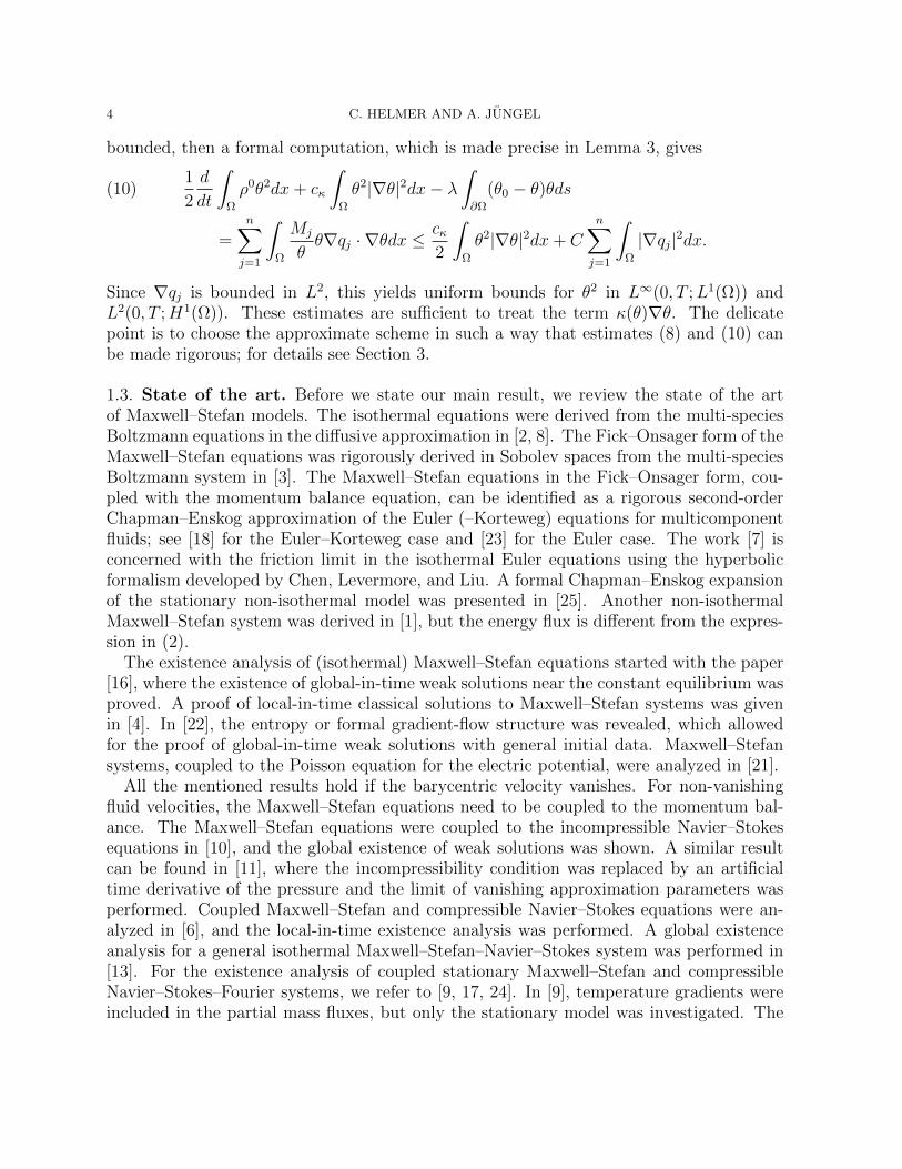
global-in-time existence of weak solutions to the transient Maxwell–Stefan–Fourier equa-tions is missing in the literature and proved in this paper for the first time.

1.4. Main result. We impose the following assumptions:

(H1) Domain: Ω ⊂ R3 is a bounded domain with a Lipschitz continuous boundary.(H2) Data: θ0 ∈ L∞(Ω), infΩ θ

0 > 0, θ0 > 0, λ ≥ 0; ρ0i ∈ L∞(Ω) satisfies 0 < ρ∗ ≤ ρ0

i ≤ ρ∗

in Ω for some ρ∗, ρ∗ > 0.

(H3) Diffusion coefficients: For i, j = 1, . . . , n, the coefficients Mij, Mj ∈ C0(Rn+ × R+)

satisfy (6)–(7) and Mij, Mi/θ are bounded functions.(H4) Heat conductivity: κ ∈ C0(R+) and there exist cκ, Cκ > 0 such that for all θ ≥ 0,

cκ(1 + θ2) ≤ κ(θ) ≤ Cκ(1 + θ2).

(H5) Reaction rates: r1, . . . , rn ∈ C0(Rn × R+) ∩ L∞(Rn × R+) satisfies∑n

i=1 ri = 0 andthere exists cr > 0 such that for all q ∈ Rn and θ > 0,

n∑i=1

ri(Πq, θ)qi ≤ −cr|Πq|2.

The bounds on ρ0 in Hypothesis (H2) are needed to derive positivity and boundedness ofthe partial mass densities. The uniform positive definiteness of the diffusion matrix on theorthogonal complement of span1 in Hypothesis (H3) provides a control on the thermo-chemical potentials, but it excludes the dilute limit, i.e. situations when the mass densitiesvanish (see Section 2). This situation is included in the recent work [14], which dealswith the isothermal case. The boundedness of Mij (and ri) is imposed for convenience;suitable growth conditions may be imposed instead but they complicate the proofs. Thegrowth condition for the heat conductivity in Hypothesis (H4) is used to derive higherintegrability of the temperature, see (10), which allows us to treat the heat flux term. Ifλ = 0, we can impose the weaker condition κ(θ) ≥ cκθ

2. Hypothesis (H5) is satisfied forthe reaction terms used in [13]. The bound for

∑ni=1 riqi gives a control on the L2(Ω)

norm of Πq. Together with the estimates for ∇(Πq) from (8), we are able to infer anH1(Ω) estimate for Πq. Hypothesis (H5) may be replaced by a Robin boundary conditionproviding an L1(∂Ω) estimate for Πq, but such a condition seems to be artificial. We notethat Hypothesis (H5) was also used in [9].

We say that (ρ, θ) is a weak solution to (1)–(4) if ρi > 0, θ > 0 a.e. in ΩT ,

ρi ∈ L∞(ΩT ) ∩ L2(0, T ;H1(Ω)) ∩H1(0, T ;H2(Ω)′), ∇qi ∈ L2(0, T ;L2(Ω)),(11)

θ ∈ L2(0, T ;H1(Ω)) ∩W 1,1(0, T ;W 1,∞(Ω)′), κ(θ)∇θ ∈ L1(ΩT );(12)

where qi = log(ρi/θ); it holds that∫ T

0

〈∂tρi, φi〉dt+

∫ T

0

∫Ω

( n∑j=1

Mij∇qj +Mi∇1

θ

)· ∇φidxdt =

∫ T

0

∫Ω

riφidxdt,(13)

∫ T

0

〈∂t(ρθ), φ0〉dt+

∫ T

0

∫Ω

κ(θ)∇θ · ∇φ0dxdt+

∫ T

0

∫Ω

n∑j=1

Mj∇qj · ∇φ0dxdt(14)


= λ

∫ T

0

∫∂Ω

(θ0 − θ)φ0dxds

for all φ1, . . . , φn ∈ L2(0, T ;H1(Ω)), φ0 ∈ L∞(0, T ;W 1,∞(Ω)) with ∇φ0 · ν = 0 on ∂Ω,and i = 1, . . . , n; and the initial conditions (4) are satisfied in the sense of H1(Ω)′ andW 1,∞(Ω)′, respectively.

Our main result is as follows.

Theorem 1 (Existence). Let Hypotheses (H1)–(H5) hold. Then there exists a weak solu-tion (ρ, θ) to (1)–(4) satisfying (11)–(14) and additionally

θ ∈ L16/3(ΩT ) ∩W 1,16/15(0, T ;W 1,16(Ω)′), κ(θ)∇θ ∈ L16/9(ΩT ).

The proof is based on a suitable approximate scheme, uniform bounds coming fromentropy estimates, and H1(Ω) estimates for the partial mass densities. More precisely, weuse two levels of approximations. First, we replace the time derivative by an implicit Eulerdiscretization to overcome issues with the time regularity. Second, we add higher-orderregularizations for the thermo-chemical potentials and the logarithm of the temperaturew = log θ to achieve H2(Ω) regularity for these variables. Since we are working in threespace dimensions, we conclude L∞(Ω) solutions, which are needed to define properly ρi =exp(w + qi).

A priori estimates are deduced from a discrete version of the entropy inequality (8). Theyare derived from the weak formulation by using qi and −e−w as test functions. The entropystructure is only preserved if we add additionally a W 1,4(Ω) regularization and some lower-order regularization in w. The properties for the heat conductivity allow us to obtainestimates for θ in H1(Ω) and for ∇ log θ in L2(Ω). As already mentioned before, the semi-definiteness property (7) only provides estimates for Πq in H1(Ω), which are not sufficientto deduce strong convergence of the mass densities. By exploiting the boundedness of ρi,identity (9) provides an estimate for qi in H1(Ω) and for ρi = θ exp(qi) in H1(Ω).

The paper is organized as follows. We explain the thermodynamical modeling of (1)–(2)in Section 2 and show that the Maxwell–Stefan formulation (5) can be always written as(1) with specific diffusion coefficients Mij and Mi. Theorem 1 is proved in Section 3.

2. Modeling

We consider an ideal fluid mixture consisting of n components with the same molar massin a fixed container Ω ⊂ R3. The balance equations for the partial mass densities ρi aregiven by

∂tρi + div(ρivi) = ri, i = 1, . . . , n,

where vi are the partial velocities and ri the reaction rates. Introducing the total massdensity ρ =

∑ni=1 ρi, the barycentric velocity v = ρ−1

∑ni=1 ρivi, and the diffusion fluxes

Ji = ρi(vi − v), we can reformulate the mass balances as

∂tρi + div(ρiv + Ji) = ri, i = 1, . . . , n.

By definition, we have∑n

i=1 Ji = 0, which means that the total mass density satisfies∂tρ + div(ρv) = 0. We assume that the barycentric velocity vanishes, v = 0, i.e., the


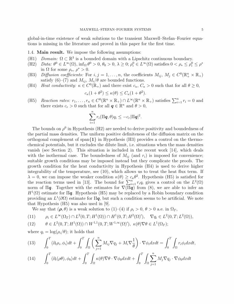
barycenter of the fluid is not moving. Consequently, the total mass density is constant intime.

Then the non-isothermal dynamics of the mixture is given by the balance equations

∂tρi + div Ji = ri, ∂tE + div Je = 0, i = 1, . . . , n,

where Je is the energy flux, and E the total energy. We assume that the diffusion fluxesare proportional to the gradients of the thermo-chemical potentials qj and the temperaturegradient (Soret effect) and that the energy flux is linear in the temperature gradient andthe gradients of qj (Dufour effect):

Ji = −n∑j=1

Mij∇qj −Mi∇1

θ, i = 1, . . . , n, Je = −κ(θ)∇θ −

n∑j=1

Mj∇qj.

The proportionality factor κ(θ) between the heat flux and the temperature gradient is theheat (or thermal) conductivity.

The thermo-chemical potentials and the total energy are determined in a thermodynam-ically consistent way from the Gibbs free energy

G = θn∑i=1

ρi(log ρi − 1)− ρθ(log θ − 1).

For simplicity, we have set the heat capacity in the free energy equal to one. The physicalentropy s, the chemical potentials µi, and the total energy E are defined by the free energyaccording to

s = −∂G∂θ

= −n∑i=1

ρi(log ρi − 1) + ρ log θ,

µi = −θ ∂s∂ρi

= θ log(ρi/θ), i = 1, . . . , n,

E = G− θ∂G∂θ

= ρθ.

We introduce the mathematical entropy h := −s and the thermo-chemical potentials qj =µj/θ = log(ρj/θ) for j = 1, . . . , n. These definitions lead to system (1)–(2). The Gibbs–Duhem relation yields the pressure p = −G +

∑ni=1 ρiµi = 0. Note that we do not need a

pressure blow-up at ρ = 0 to exclude vacuum or a superlinear growth in θ to control thetemperature.

If the molar masses mi of the components are not the same, we need to modify the Gibbsfree energy according to [9, Remark 1.2]

G = θn∑i=1

ρimi

(log

ρimi

− 1

)− cWρθ(log θ − 1),

where cW > 0 is the heat capacity. For simplicity, we have set mi = 1 and cW = 1.


We already mentioned that the Maxwell–Stefan equations are usually formulated as

(15) ∂tρi + div Ji = ri, di = −n∑j=1

bijρiρj

(Jiρi− Jjρj

), i = 1, . . . , n.

According to [5, (176)], the driving forces are given by di = ρiθ∇qi+Diθ−1∇θ. The function

Di is the sum of the partial enthalpy [5, (85)] and the phenomenological thermal diffusivity[5, (106)]. The partial enthalpy of the ith species is the sum of the partial internal energyρiθ and the partial pressure ρiθ. Thus, choosing a vanishing thermal diffusivity, we findthat Di = 2ρiθ, and this gives the expression di = ∇(ρiθ) also found in [19]. If (bij) issymmetric, we see that

∑ni=1 di = 0.

We show that (15) implies (1) for a specific choice of Mij and Mi. This result is well-known in the thermodynamic community (see, e.g., [5, (183)]); here, we make explicit thehypotheses to achieve this result. Namely, we need a property for the coefficients bij in(5). We suppose that the homogeneous system

(16)n∑j=1

bijρiρj(ui − uj) = 0, i = 1, . . . , n,

has only solutions in span1, where 1 = (1, . . . , 1) ∈ Rn. This holds true if, for instance,bij = bji > 0 for i, j = 1, . . . , n.

Proposition 2. Let bij = bji ≥ 0 for i, j = 1, . . . , n and let the linear system (16) has onlysolutions in span1. Then (5) can be written as (1) with

(17) Mij = Nijρjθ, Mi = −2n∑k=1

Nikρkθ2 for i, j = 1, . . . , n,

where Nij depends only on (bij) and ρ, and Mij and Mi satisfy (6).

Proof. It follows from the property on the linear system (16) that

(18) −n∑j=1

bijρiρj

(Jiρi− Jjρj

)= di, i = 1, . . . , n,

subject to∑n

i=1 Ji = 0, has the unique solution [18, Lemma 1]

(19) Ji = ρiui = −n−1∑j,k=1

(δijρi −

ρiρjρ

)cjkdk, i = 1, . . . , n− 1,

and Jn = −∑n−1

i=1 Ji. The coefficients cjk depend only on (bij). The diffusion fluxes can be

reformulated as Ji = −∑n−1

k=1 Dikdk after setting

Dik =n−1∑j=1

(δijρi − ρiρj/ρ)cjk, i, k = 1, . . . , n− 1.


The aim is to formulate Ji = −∑n

k=1Nikdk for some coefficients Nik. Define

Nik = Dik −1

n

n−1∑j=1

Dij, i, j = 1, . . . , n− 1.

Then (Nik) solves the linear system

Nij +n−1∑k=1

Nik = Dij, j = 1, . . . , n− 1,

for each fixed i ∈ 1, . . . , n− 1. We extend (Nij) to an n× n matrix by defining

Nnj = −n−1∑k=1

Nkj, j = 1, . . . , n− 1,

Nin = −n−1∑k=1

Nik, i = 1, . . . , n.

It follows from dn = −∑n−1

i=1 di that

Ji = −n−1∑k=1

Dikdk = −n−1∑k=1

(Nik +

n−1∑j=1

Nij

)dk = −

n−1∑k=1

(Nik −Nin)dk

= −n∑k=1

Nikdk −Nindn = −n∑k=1

Nikdk.

Since dk = ∇(ρkθ) = ρkθ(∇qk − 2θ∇(1/θ)), we find that

Ji = −n∑k=1

Nikρkθ∇qk + 2n∑k=1

Nikρkθ2∇1

θ.

Setting Mij = Nijρjθ for i, j = 1, . . . , n and Mi = −2∑n

k=1Nikρkθ2, we arrive to the

second expression in (1). The coefficients satisfy for j = 1, . . . , n,n∑i=1

Mij =

( n∑i=1

Nij

)ρjθ = 0,

n∑i=1

Mi = −2n∑k=1

( n∑i=1

Nik

)ρkθ

2 = 0.

This shows the proposition.

We observe that the diffusion fluxes in (1) can be written as (19) under the conditions∑ni=1∇(ρiθ) = 0 and

(20)n∑j=1

Mij = −Mi

θ,

n∑j=1

Mij

ρj= 0 for i = 1, . . . , n.

Equations (20) are valid for the Maxwell–Stefan equations in Fick–Onsager form thatare derived from the Boltzmann equation in the limit of small Knudsen numbers; seeformulas (A13) and (A15) in [25]. To derive formulation (19), we set dj := ∇(ρjθ) and


Nij := Mij/(ρjθ). Then∑n

j=1 Nij = 0. Using ∇qj = dj/(ρjθ) + 2ρjθ2∇(1/θ), condition

(20), and∑n

i=1 di = 0, we compute

Ji = −n∑j=1

Nijdj −( n∑

j=1

Nijρjθ2 +Mi

)∇1

θ= −

n∑j=1

Nijdj

= −n−1∑j=1

Nijdj −Nindn = −n−1∑j=1

(Nij −Nin)dj = −n−1∑j=1

(Nij +

n−1∑k=1

Nik

)dj.

Thus, setting Dij = Nij +∑n−1

k=1 Nik for i, j = 1, . . . , n− 1, we obtain Ji = −∑n−1

j=1 Dijdj.

The matrix with coefficients Rij = δijρi−ρiρj/ρ is invertible with inverse Qij = δijρ−1i +

ρ−1n for i, j = 1, . . . , n − 1; see the proof of [18, Lemma 1]. We introduce the matrixcij =

∑n−1k=1 QikDkj. Then Dik =

∑n−1j=1 Rijcjk and

Ji = −n−1∑k=1

Dikdk = −n−1∑j,k=1

Rijcjkdk = −n−1∑j,k=1

(δijρi −

ρiρjρ

)cjkdk,

which equals (19).

3. Proof of Theorem 1

The idea of the proof is to approximate equations (1)–(4) by an implicit Euler schemeand to add some higher-order regularizations in space for the variables q and w = log θ.The de-regularization limit is based on the compactness coming from the entropy estimates.

Set w0 = log θ0, ε > 0, N ∈ N, and τ = T/N > 0. Let (q, w) ∈ L∞(Ω;Rn+1) be givenand define the approximate scheme

0 =1

τ

∫Ω

(ρi − ρi)φidx+

∫Ω

( n∑j=1

Mij(ρ, ew)∇qj −Mi(ρ, e

w)e−w∇w)· ∇φidx(21)

+ ε

∫Ω

(D2qi : D2φi + qiφi

)dx−

∫Ω

ri(ρ, ew)φidx,

0 =1

τ

∫Ω

(E − E)φ0dx+

∫Ω

(κ(θ)∇θ +

n∑j=1

Mj(ρ, ew)∇qj

)· ∇φ0dx(22)

− λ∫∂Ω

(θ0 − θ)φ0ds+ ε

∫Ω

ew(D2w : D2φ0 + |∇w|2∇w · ∇φ0

)dx

+ ε

∫Ω

(ew0 + ew)(w − w0)φ0dx

for test functions φi ∈ H2(Ω), i = 0, . . . , n. Here, D2u is the Hessian matrix of thefunction u, “:” denotes the Frobenius matrix product, and E = ρθ, E = ρθ. The lower-order regularization ε(ew0 + ew)(w−w0) yields an L2(Ω) estimate for w. Furthermore, thehigher-order regularization guarantees that qi, w ∈ H2(Ω) → L∞(Ω), while the W 1,4(Ω)


regularization term for w allows us to estimate the higher-order terms when using the testfunction e−w0 − e−w.

Step 1: solution of the linearized approximate problem. In order to define the fixed-point operator, we need to solve a linearized problem. To this end, let y∗ = (q∗, w∗) ∈W 1,4(Ω;Rn+1) and σ ∈ [0, 1] be given. We want to find the unique solution y = (q, w) ∈H2(Ω;Rn+1) to the linear problem

(23) a(y, φ) = σF (φ) for all φ = (φ0, . . . , φn) ∈ H2(Ω;Rn+1),

where

a(y, φ) =

∫Ω

n∑i,j=1

Mij(ρ∗, ew

∗)∇qj · ∇φidx+

∫Ω

κ(ew∗)ew

∗∇w · ∇φ0dx

+ ε

∫Ω

n∑i=1

(D2qi : D2φi + qiφi

)dx

+ ε

∫Ω

ew∗(D2w : D2φ0 + |∇w∗|2∇w · ∇φ0

)dx,

F (φ) = −1

τ

∫Ω

n∑i=1

(ρ∗i − ρi)φidx−1

τ

∫Ω

(E∗ − E)φ0dx+ λ

∫∂Ω

(ew0 − ew∗)φ0dx

+

∫Ω

n∑i=1

Mi(ρ∗, ew

∗)e−w

∗∇w∗ · ∇φidx−∫

Ω

n∑j=1

Mj(ρ∗, ew

∗)∇q∗j · ∇φ0dx

+

∫Ω

n∑i=1

ri(ρ∗, ew

∗)φidx− ε

∫Ω

(ew0 + ew∗)(w∗ − w0)φ0dx

and ρ∗i = ew∗+q∗i , ρ∗ =

∑ni=1 ρ

∗i , E

∗ = ρ∗ew∗. By Hypothesis (H3) and the generalized

Poincare inequality [26, Chap. 2, Sec. 1.4], we have

a(y, y) ≥ ε

∫Ω

(|D2q|2 + |q|2

)dx+ ε

∫Ω

(|D2w|2 + w2)dx ≥ εC(‖q‖2H2(Ω) + ‖w‖2

H2(Ω)).

Thus, a is coercive. Moreover, a and F are continuous on H2(Ω;Rn+1). The Lax–Milgramlemma shows that (23) possesses a unique solution (q, w) ∈ H2(Ω;Rn+1).

Step 2: solution of the approximate problem. The previous step shows that the fixed-point operator S : W 1,4(Ω;Rn+1)× [0, 1]→ W 1,4(Ω;Rn+1), S(y∗, σ) = y, where y = (q, w)solves (23), is well defined. It holds that S(y, 0) = 0, S is continuous, and since S mapsto H2(Ω;Rn+1), which is compactly embedded into W 1,4(Ω;Rn+1), it is also compact. Itremains to determine a uniform bound for all fixed points y of S(·, σ), where σ ∈ (0, 1].Let y be such a fixed point. Then y ∈ H2(Ω;Rn+1) solves (23) with (q∗, w∗) replaced byy = (q, w). With the test functions φi = qi for i = 1, . . . , n and φ0 = e−w0 − e−w (we needthis test function since φ0 = −e−w does not allow us to control the lower-order term), we


obtain

0 =σ

τ

∫Ω

n∑i=1

(ρi − ρi)qidx+σ

τ

∫Ω

(E − E)(−e−w)dx+σ

τ

∫Ω

(E − E)e−w0dx

+

∫Ω

n∑i,j=1

Mij∇qi · ∇qjdx+

∫Ω

κ(ew)ew∇w · ∇(−e−w)dx− σ∫

Ω

n∑i=1

riqidx

− σ∫

Ω

n∑j=1

Mje−w∇w · ∇qjdx+ σ

∫Ω

n∑j=1

Mj∇qj · ∇(−e−w)dx

− σλ∫∂Ω

(ew0 − ew)(e−w0 − e−w)dx+ ε

∫Ω

n∑i=1

(|D2qi|2 + q2

i

)dx

+ ε

∫Ω

(ew0 + ew)(w − w0)(e−w0 − e−w)dx

+ ε

∫Ω

(|D2w|2 +D2w : ∇w ⊗∇w + |∇w|4

)dx

=: I1 + · · ·+ I12.

We see immediately that I7 + I8 = 0. Furthermore,

I1 + I2 =σ

τ

∫Ω

( n∑i=1

(ρi − ρi)∂h

∂ρi+ (θ − θ)∂h

∂θ

)dx.

The function (ρ, θ) 7→ h(ρ, θ) is convex since, by the Cauchy–Schwarz inequality, for anyz = (z, zn+1) = (z1, . . . , zn, zn+1) ∈ Rn+1,

z>D2hz =n∑i=1

z2i

ρi− 2

θ

n∑i=1

zizn+1 +ρ

θ2z2n+1 ≥

n∑i=1

(1

ρi− 1

ρ

)z2i ≥ 0.

This shows that

h(ρ, θ)− h(ρ, θ) ≤n∑i=1

∂h

∂ρi(ρ, θ)(ρi − ρi) +

∂h

∂θ(ρ, θ)(θ − θ)

and consequently,

I1 + I2 ≥σ

τ

∫Ω

(h(ρ, θ)− h(ρ, θ)

)dx.

By Hypotheses (H3) and (H5),

I4 ≥ cM

∫Ω

|∇Πq|2dx, I6 ≥ σcr

∫Ω

|Πq|2dx.

This gives an H1(Ω) bound for Πq. Next, we have

I5 =

∫Ω

κ(ew)|∇w|2dx, I9 = 2σλ

∫∂Ω

(cosh(w0 − w)− 1)ds ≥ 0,


I11 = 2ε

∫Ω

(w − w0) sinh(w − w0)dx ≥ ε

∫Ω

(w − w0)2dx,

I12 =ε

2

∫Ω

(|D2w|2 + |D2w −∇w ⊗∇w|2 + |∇w|4

)dx.

Summarizing these estimates and applying the generalized Poincare inequality, we arriveat the discrete entropy inequality

σ

τ

∫Ω

(h(ρ, θ) + e−w0E

)dx+ σ

∫Ω

(cM |∇Πq|2 + cr|Πq|2

)dx+

∫Ω

κ(ew)|∇w|2dx

+ εC(‖q‖2

H2(Ω) + ‖w‖2H2(Ω) + ‖w‖4

W 1,4(Ω)

)≤ σ

τ

∫Ω

(h(ρ, θ) + e−w0E

)dx.(24)

This estimate gives a uniform bound for (q, w) in H2(Ω;Rn+1) and consequently also inW 1,4(Ω; Rn+1), which proves the claim. We infer from the Leray–Schauder fixed-pointtheorem that there exists a solution (q, w) to (21)–(22).

Step 3: temperature estimate. We need a better estimate for the temperature. Thefollowing result gives a conditional estimate. We prove below that∇q is uniformly boundedin L2(Ω), yielding an unconditional estimate.

Lemma 3. Let (ρ, w) be a solution to (21)–(22) and set θ = ew. Then there exists aconstant C > 0 independent of ε and τ such that

1

τ

∫Ω

ρ0θ2dx+1

2

∫Ω

κ(θ)|∇θ|2dx ≤ C +1

τ

∫Ω

ρ0θ2dx+ Cn∑j=1

∫Ω

|∇qj|2dx.

Proof. We use the test function θ in (22). Observing that (E − E)θ = ρ0(θ − θ)θ ≥(ρ0/2)(θ2 − θ2) and that κ(θ) ≥ cκ(1 + θ2) by Hypothesis (H4), we find that

1

2τ

∫Ω

ρ0(θ2 − θ2)dx+1

2

∫Ω

κ(θ)|∇θ|2dx+cκ2

∫Ω

θ2|∇θ|2dx− λ∫∂Ω

(θ0 − θ)θdx

≤ −n∑j=1

∫Ω

Mj∇qj · ∇θdx− ε∫

Ω

θ(D2 log θ : D2θ + |∇ log θ|2∇ log θ · ∇θ)dx

− ε∫

Ω

(θ0 + θ)(log θ − log θ0)θdx

=: J1 + J2 + J3.(25)

Since Mj/θ is assumed to be bounded,

J1 ≤cκ2

∫Ω

θ2|∇θ|2dx+ Cn∑j=1

∫Ω

|∇qj|2dx.

Furthermore,

J2 = −ε∫

Ω

(− 1

θ∇θ ·D2θ∇θ + |D2θ|2 +

1

θ2|∇θ|4

)dx


= −ε2

∫Ω

(|D2θ|2 +

1

θ2|∇θ|4 +

∣∣∣∣D2θ − 1

θ∇θ ⊗∇θ

∣∣∣∣2)dx ≤ 0.

The last integral J3 is bounded since −θ2 log θ is the dominant term. The last term onthe left-hand side of (25) is bounded from below by −(λ/2)

∫∂Ωθ2

0dx, which finishes theproof.

Remark 4. Better estimates can be derived if we assume that κ(θ) ≥ cκ(1 + θα+1) forα ∈ (1, 2). Indeed, using θα as a test function in (22), we find that

1

τ

∫Ω

ρ0(θ − θ)θαdx+ αcκ

∫Ω

θ2α|∇θ|2dx− λ∫∂Ω

(θ0 − θ)θαdx

≤ −αn∑j=1

∫Ω

Mjθα−1∇qj · ∇θdx− ε

∫Ω

(θ0 + θ)(log θ − log θ0)θαdx

− ε∫

Ω

θ(D2 log θ : D2θα + |∇ log θ|2∇ log θ · ∇θα

)dx

=: J4 + J5 + J6.(26)

A tedious but straightforward computation shows that J6 ≥ 0 if α ∈ (1, 2). Furthermore,since Mj/θ is bounded,

J4 ≤αcκ2

∫Ω

θ2α|∇θ|2dx+ Cn∑j=1

∫Ω

|∇qj|2dx.

The first integral on the right-hand side is controlled by the left-hand side of (26). Thisyields a bound for θα+1 ∈ L∞(0, T ;L1(Ω)) ∩ L2(0, T ;H1(Ω)) ⊂ L8/3(ΩT ) (see Lemma 7)and consequently θ ∈ L8(α+1)/3(ΩT ), which is better than the result in Lemma 7.

Step 4: uniform estimates. Let (qk, wk) be a solution to (21)–(22) for given qk−1 = qand wk−1 = w, where k ∈ N. We set θk = exp(wk), ρki = exp(wk + qki ) for i = 1, . . . , n,and Ek = ρkθk. Recall that ρ0 =

∑ni=1 ρ

ki does not depend on k ∈ N. We introduce

piecewise constant functions in time. For this, let ρ(τ)i (x, t) = ρki (x), θ(τ)(x, t) = θk(x),

and q(τ)i (x, t) = qki (x) for x ∈ Ω, t ∈ ((k − 1)τ, kτ ], k = 1, . . . , N . At time t = 0, we set

ρ(τ)i (x, 0) = ρ0

i (x) and θ(τ)(x, 0) = θ0(x) for x ∈ Ω. Furthermore, we introduce the shift

operator (στρ(τ)i )(x, t) = ρk−1

i (x) for x ∈ Ω, t ∈ ((k − 1)τ, kτ ]. Let ρ(τ) = (ρ(τ)1 , . . . , ρ

(τ)n ).

Then (ρ(τ), θ(τ)) solves (see (21)–(22))

0 =1

τ

∫ T

0

∫Ω

(ρ(τ)i − στρ

(τ)i )φidxdt(27)

+

∫ T

0

∫Ω

( n∑j=1

Mij(ρ(τ), θ(τ))∇q(τ)

j +Mi(ρ(τ), θ(τ))∇ 1

θ(τ)

)· ∇φidxdt

+ ε

∫ T

0

∫Ω

(D2q

(τ)i : D2φi + qiφi

)dxdt−

∫ T

0

∫Ω

ri(ρ(τ), θ(τ))φidxdt,


0 =1

τ

∫ T

0

∫Ω

(E(τ) − στE(τ))φ0dxdt− λ∫ T

0

∫∂Ω

(θ0 − θ(τ))φ0dsdt(28)

+

∫ T

0

∫Ω

(κ(θ(τ))∇θ(τ) +

n∑j=1

Mj(ρ(τ), θ(τ))∇q(τ)

j

)· ∇φ0dxdt

+ ε

∫ T

0

∫Ω

θ(τ)(D2 log θ(τ) : D2φ0 + |∇ log θ(τ)|2∇ log θ(τ) · ∇φ0

)dxdt

+ ε

∫ T

0

∫Ω

(θ0 + θ(τ))(log θ(τ) − log θ0)φ0dxdt.

The discrete entropy inequality (24), the L∞ bound for ρ(τ)i , and the property E(τ) =

ρ(τ)θ(τ) = ρ0θ(τ) ≥ ρ∗θ(τ) imply the following uniform bounds:

‖ρ(τ)i ‖L∞(0,T ;L∞(Ω)) + ‖θ(τ)‖L∞(0,T ;L1(Ω)) ≤ C,

‖Πq(τ)‖L2(0,T ;H1(Ω)) + ‖κ(θ(τ))1/2∇ log θ(τ)‖L2(ΩT ) ≤ C,

ε1/2‖q(τ)i ‖L2(0,T ;H2(Ω)) + ε1/2‖ log θ(τ)‖L2(0,T ;H2(Ω)) ≤ C,

ε1/4‖ log θ(τ)‖L4(0,T ;W 1,4(Ω)) ≤ C,

for all i = 1, . . . , n, where C > 0 is independent of ε and τ . Hypothesis (H4) yields

‖∇θ(τ)‖L2(ΩT ) + ‖∇ log θ(τ)‖L2(ΩT ) ≤ C.

Then the L∞(0, T ;L1(Ω)) bound for θ(τ) and the Poincare–Wirtinger inequality show that

‖θ(τ)‖L2(0,T ;H1(Ω)) ≤ C.

We proceed by proving more uniform estimates. The following lemma is the key result.

Lemma 5. There exists C > 0 independent of ε and τ such that

(29) ‖ρ(τ)i ‖L2(0,T ;H1(Ω)) + ‖∇q(τ)

i ‖L2(0,T ;L2(Ω)) ≤ C.

Proof. We infer from ρ0 =∑n

i=1 ρ(τ)i and ρ

(τ)i = θ(τ) exp(q

(τ)i ) that

∇ρ0 =n∑i=1

∇ρ(τ)i =

n∑i=1

ρ(τ)i (∇ log θ(τ) +∇q(τ)

i )

= ρ0∇ log θ(τ) +n∑i=1

ρ(τ)i ∇

(q

(τ)i −

1

n

n∑j=1

q(τ)j

)+

1

n

n∑i=1

ρ(τ)i

n∑j=1

∇q(τ)j

= ρ0∇ log θ(τ) +n∑i=1

ρ(τ)i (∇Πq(τ))i +

1

nρ0

n∑j=1

∇q(τ)j .


Since (ρ(τ)i ) is bounded in L∞(ΩT ) and (∇ log θ(τ)) and (∇Πq(τ)) are bounded in L2(ΩT ),

we conclude that

1

n

n∑j=1

∇q(τ)j = ∇ log ρ0 −∇ log θ(τ) − 1

ρ0

n∑i=1

ρ(τ)i ∇

(Πq(τ)

)i

is uniformly bounded in L2(ΩT ). It follows that

∇q(τ)i = ∇

(Πq(τ)

)i+

1

n

n∑j=1

∇q(τ)j

is uniformly bounded in L2(ΩT ) too. This shows that ∇ρ(τ)i = ρ

(τ)i (∇ log θ(τ) + ∇q(τ)

i ) isuniformly bounded in L2(ΩT ), finishing the proof.


(30) ‖θ(τ)‖L∞(0,T ;L2(Ω)) + ‖∇(θ(τ))2‖L2(ΩT ) ≤ C.

Proof. Lemma 3 shows that for t ∈ [0, T ],∫Ω

ρ0((θ(τ))2 − θ0)2

)dx+

∫ t

0

∫Ω

(θ(τ))2|∇θ(τ)|2dxdt

≤ C + C

∫ T

0

∫Ω

|∇q|2dxdt.

The last term is bounded thanks to Lemma 5. Therefore, the right-hand side is uniformlybounded. Using ρ0 ≥ ρ∗ > 0, the lemma is proved.

Lemma 7. There exists C > 0 independent of ε and τ such that (θ(τ)) is bounded inL16/3(ΩT ).

Proof. We know from Lemma 6 that ∇(θ(τ))2 is uniformly bounded in L2(ΩT ) and (θ(τ))2 isuniformly bounded in L2(0, T ;L1(Ω)). We deduce from the Poincare–Wirtinger inequalitythat (θ(τ))2 is uniformly bounded in L2(ΩT ) and consequently also in L2(0, T ;H1(Ω)) ⊂L2(0, T ;L6(Ω)). This shows that (θ(τ)) is bounded in L4(0, T ;L12(Ω)). By interpolationwith 1/r = α/12 + (1− α)/2 and rα = 4,

‖θ(τ)‖rLr(ΩT ) =

∫ T

0

‖θ(τ)‖rLr(Ω)dt ≤∫ T

0

‖θ(τ)‖rαL12(Ω)‖θ(τ)‖r(1−α)

L2(Ω))dt

≤ ‖θ(τ)‖r(1−α)

L∞(0,T ;L2(Ω))

∫ T

0

‖θ(τ)‖4L12(Ω)dt ≤ C.

The solution of 1/r = α/12 + (1− α)/2 and rα = 4 is α = 3/4 and r = 16/3.


(31) τ−1‖ρ(τ)i − στρ

(τ)i ‖L2(0,T ;H2(Ω)′) + τ−1‖θ(τ) − στθ(τ)‖L16/15(0,T ;W 1,16(Ω)′) ≤ C.


Proof. Let φ0 ∈ L16(0, T ;W 1,16(Ω)), φ1, . . . , φn ∈ L2(0, T ;H2(Ω)) and set M(τ)i = Mi(ρ

(τ),

θ(τ)), r(τ)i = ri(ρ

(τ), θ(τ)) for i = 1, . . . , n. It follows from (27)–(28) and Hypotheses (H3)–(H5) that

1

τ

∣∣∣∣ ∫ T

0

∫Ω

(ρ(τ)i − στρ

(τ)i )φidxdt

∣∣∣∣ ≤ C‖∇q(τ)‖L2(ΩT )‖∇φ‖L2(ΩT )

+n∑i=1

‖M (τ)i /θ(τ)‖L∞(ΩT )‖∇ log θ(τ)‖L2(ΩT )‖∇φ‖L2(ΩT )

+ ε‖q(τ)‖L2(0,T ;H2(Ω))‖φ‖L2(0,T ;H2(Ω)) + ‖r(τ)‖L2(ΩT )‖φ‖L2(ΩT )

≤ C‖φ‖L2(0,T ;H2(Ω)),

and

1

τ

∣∣∣∣ ∫ T

0

∫Ω

(E(τ) − στE(τ))φ0dxdt

∣∣∣∣≤ C + C‖θ(τ)‖L8/3(ΩT )‖∇(θ(τ))2‖L2(ΩT )‖∇φ0‖L8(ΩT )

+n∑j=1

‖M (τ)j /θ(τ)‖L∞(ΩT )‖θ(τ)‖L8/3(ΩT )‖∇q

(τ)j ‖L2(ΩT )‖∇φ0‖L8(ΩT )

+ λ‖θ0 − θ(τ)‖L8/7(0,T ;L8/7(∂Ω))‖φ0‖L8(0,T ;L8(∂Ω))

+ ε‖θ(τ)‖L3(ΩT )‖ log θ(τ)‖L2(0,T ;H2(Ω))‖∇φ0‖L6(ΩT )

+ ε‖θ(τ)‖L16/3(ΩT )‖∇ log θ(τ)‖3L4(ΩT )‖∇φ0‖L16(ΩT )

+ εC(1 + ‖θ(τ) log θ(τ)‖L2(ΩT )

)‖φ0‖L2(ΩT ) ≤ C‖φ0‖L16(0,T ;W 1,16(Ω)).

Since |E(τ) − στE(τ)| = ρ0|θ(τ) − στθ(τ)| ≥ ρ∗|θ(τ) − στθ(τ)|, this concludes the proof.

Step 4: limit (ε, τ)→ 0. Estimates (29)–(31) allow us to apply the Aubin–Lions lemmain the version of [12]. Thus, there exist subsequences that are not relabeled such that as(ε, τ)→ 0,

(32) ρ(τ)i → ρi, θ(τ) → θ strongly in L2(ΩT ), i = 1, . . . , n.

The L∞(ΩT ) bound for (ρ(τ)i ) and the L16/3(ΩT ) bound for (θ(τ)) imply the stronger con-

vergences

ρ(τ)i → ρi strongly in Lr(ΩT ) for all r <∞,θ(τ) → θ strongly in Lη(ΩT ) for all η < 16/3.

The uniform bounds also imply that, up to subsequences,

ρ(τ)i ρi weakly in L2(0, T ;H1(Ω)),

θ(τ) θ weakly in L2(0, T ;H1(Ω)),

∇q(τ)i ∇qi weakly in L2(0, T ;L2(Ω)),


τ−1(ρ(τ)i − στρ

(τ)i ) ∂tρi weakly in L2(0, T ;H2(Ω)′),

τ−1(θ(τ) − στθ(τ)) ∂tθ weakly in L16/15(0, T ;W 2,16(Ω)′),

Moreover, as (ε, τ)→ 0,

ε log θ(τ) → 0, εq(τ)i → 0 strongly in L2(0, T ;H2(Ω)).

We deduce from the linearity and boundedness of the trace operator H1(Ω) → H1/2(∂Ω)that

θ(τ) θ weakly in L2(0, T ;H1/2(∂Ω)).

Using the compact embedding H1/2(∂Ω) → L2(∂Ω), this gives

θ(τ) → θ strongly in L2(0, T ;L2(∂Ω)).

Next, we prove that ρi and θ are positive a.e. The functions ρ(τ)i = exp(w

(τ)i + q

(τ)i ) and

θ(τ) = exp(w(τ)i ) are positive in ΩT and therefore, the limits ρi and θ are nonnegative. We

claim that ρ and θ is even positive a.e. Indeed, by the Chebyshev inequality, we have forany δ ∈ (0, 1),

meas(x, t) : θ(τ)(x, t) ≤ δ = meas(x, t) : − log θ(τ)(x, t) ≥ − log δ

≤ C

− log δ

∫ T

0

∫θ(τ)≤δ

(− log θ(τ))dxdt ≤ C

− log δ.

It follows in the limit δ → 0 and (ε, τ) → 0 that meas(x, t) : θ(x, t) = 0 = 0. Hence,

θ > 0 a.e. in ΩT . Furthermore, since q(τ)i is integrable and log ρ

(τ)i = q

(τ)i + log θ(τ), the

same argument shows that

meas(x, t) : ρ(τ)i (x, t) ≤ δ = meas(x, t) : − log ρ

(τ)i (x, t) ≥ − log δ

≤ C

− log δ

∫ T

0

∫ρ(τ)i ≤δ

(− log ρ(τ)i )dxdt

≤ C

− log δ

∫ T

0

∫Ω

(|qi|+ | log θ|

)dxdt ≤ C

− log δ,

and in the limit δ → 0 and (ε, τ)→ 0, we infer again that ρi > 0 a.e. in ΩT .By assumption, Mij(ρ

(τ), θ(τ)) and Mj(ρ(τ), θ(τ))/θ(τ) are bounded. Then the strong

convergences imply that these sequences are converging in Lq(ΩT ) for q < ∞, and thelimits can be identified. Thus,

Mij(ρ(τ), θ(τ))→Mij(ρ, θ) strongly in Lq(ΩT ),

Mj(ρ(τ), θ(τ))/θ(τ) →Mj(ρ, θ)/θ strongly in Lq(ΩT ) for all q <∞.

This shows that

Mj(ρ(τ), θ(τ)) =

1

θ(τ)Mj(ρ

(τ), θ(τ))θ(τ) → 1

θMj(ρ, θ)θ = Mj(ρ, θ)


strongly in Lη(ΩT ) for η < 16/3 and

1

(θ(τ))2Mj(ρ

(τ), θ(τ))→ 1

θ2Mj(ρ, θ)

strongly in Lη(ΩT ) for η < 8/3.

The a.e. convergence of (ρ(τ)i ), (θ(τ)) implies that

q(τ)i = log ρ

(τ)i − log θ(τ) → log ρi − log θ =: qi a.e. in ΩT

and consequently, ∇q(τ)i → ∇qi weakly in L2(ΩT ). We conclude that

Mij(ρ(τ), θ(τ))∇q(τ)

j Mij(ρ, θ)∇qj weakly in Lη(ΩT ), η ≤ 2,

Mj(ρ(τ), θ(τ))∇q(τ)

j Mj(ρ, θ)∇qj weakly in Lη(ΩT ), η ≤ 2,

Mj(ρ(τ), θ(τ))∇ 1

θ(τ) − 1

θ2Mj(ρ, θ)∇θ weakly in Lη(ΩT ), η ≤ 2.

Moreover, by Hypothesis (H5),

ri(Πq(τ), θ(τ))→ ri(Πq, θ) strongly in Lη(ΩT ), η <∞.

These convergences allow us to perform the limit (ε, τ) → 0 in (27)–(28) to obtain (13)–

(14). Finally, we can show as in [20, p. 1980f] that the linear interpolant ρ(τ)i of ρ

(τ)i and the

piecewise constant function ρ(τ)i converge to the same limit, which leads to ρ0

i = ρ(τ)i (0)

ρi(0) weakly in H1(Ω)′. Thus, the initial datum ρi(0) = ρ0i is satisfied in the sense of

H2(Ω)′. Similarly, (ρθ)(0) = ρ0θ0 in the sense of W 1,16(Ω)′. This finishes the proof.

References

[1] B. Anwasia, M. Bisi, F. Salvarani, and A. J. Soares. On the Maxwell–Stefan diffusion limit for areactive mixture of polyatomic gases in non-isothermal setting. Kinetic Related Models 13 (2020),63–95.

[2] A. Bondesan and M. Briant. Stability of the Maxwell–Stefan system in the diffusion asymptotics ofthe Boltzmann multi-species equation. Submitted for publication, 2019. arXiv:1910.08357.

[3] M. Briant and B. Grec. Rigorous derivation of the Fick cross-diffusion system from the multi-speciesBoltzmann equation in the diffusive scaling. Submitted for publication, 2020. arXiv:2003.07891.

[4] D. Bothe. On the Maxwell–Stefan equations to multicomponent diffusion. In: J. Escher et al. (eds).Parabolic Problems. Progress in Nonlinear Differential Equations and their Applications, pp. 81–93.Springer, Basel, 2011.

[5] D. Bothe and W. Dreyer. Continuum thermodynamics of chemically reacting fluid mixtures. ActaMech. 226 (2015), 1757–1805.

[6] D. Bothe and P.-E. Druet. Mass transport in multicomponent compressible fluids: Local and globalwell-posedness in classes of strong solutions for general class-one models. Submitted for publication,2020. arXiv:2001.08970.

[7] L. Boudin, B. Grec, and V. Pavan. Diffusion models for mixtures using a stiff dissipative hyperbolicformalism. J. Hyperbol. Eqs. 16 (2019), 293–312.

[8] L. Boudin, B. Grec, M. Pavic, and F. Salvarani. Diffusion asymptotics of a kinetic model for gaseousmixtures. Kinetic Related Models 6 (2013), 137–157.


[9] M. Bulicek, A. Jungel, M. Pokorny, and N. Zamponi. Existence analysis of a stationary compressiblefuid model for heat-conducting and chemically reacting mixtures. Submitted for publication, 2020.arXiv:2001.06082.

[10] X. Chen and A. Jungel. Analysis of an incompressible Navier–Stokes–Maxwell–Stefan system. Com-mun. Math. Phys. 340 (2015), 471–497.

[11] M. Dolce and D. Donatelli. Artificial compressibility method for the Navier–Stokes–Maxwell–Stefansystem. J. Dyn. Diff. Eqs., 2019. https://doi.org/10.1007/s10884-019-09808-4.

[12] M. Dreher and A. Jungel. Compact families of piecewise constant functions in Lp(0, T ;B). Nonlin.Anal. 75 (2012), 3072–3077.

[13] W. Dreyer, P.-E. Druet, P. Gajewski, and C. Guhlke. Analysis of improved Nernst–Planck–Poissonmodels of compressible isothermal electrolytes. Part I. Derivation of the model and survey of theresults. To appear in Z. Angew. Math. Phys., 2020.

[14] P.-E. Druet. A theory of generalised solutions for ideal gas mixtures with Maxwell–Stefan diffusion.Submitted for publication, 2020. WIAS Preprint no. 2700, WIAS Berlin, Germany.

[15] E. Feireisl and A. Novotny. Singular Limits in Thermodynamics of Viscous Flows. Birkhauser, Basel,2009.

[16] V. Giovangigli and M. Massot. The local Cauchy problem for multicomponent flows in full vibrationalnon-equilibrium. Math. Meth. Appl. Sci. 21 (1998), 1415–1439.

[17] V. Giovangigli, M. Pokorny, and E. Zatorska. On the steady flow of reactive gaseous mixture. Analysis(Berlin) 35 (2015), 319–341.

[18] X. Huo, A. Jungel, and A. Tzavaras. High-friction limits of Euler flows for multicomponent systems.Nonlinearity 32 (2019), 2875–2913.

[19] H. Hutridurga and F. Salvarani. Existence and uniqueness analysis of a non-isothermal cross-diffusionsystem of Maxwell–Stefan type. Appl. Math. Lett. 75 (2018), 108–113.

[20] A. Jungel. The boundedness-by-entropy method for cross-diffusion systems. Nonlinearity 28 (2015),1963–2001.

[21] A. Jungel and O. Leingang. Convergence of an implicit Euler Galerkin scheme for Poisson–Maxwell–Stefan systems. Adv. Comput. Math. 45 (2019), 1469–1498.

[22] A. Jungel and I. V. Stelzer. Existence analysis of Maxwell–Stefan systems for multicomponent mix-tures. SIAM J. Math. Anal. 45 (2013), 2421–2440.

[23] L. Ostrowski and C. Rohde. Compressible multi-component flow in porous media with Maxwell–Stefandiffusion. To appear in Math. Meth. Appl. Sci., 2020. arXiv:1905.08496.

[24] T. Piasecki and M. Pokorny. Weak and variational entropy solutions to the system describing steadyflow of a compressible reactive mixture. Nonlin. Anal. 159 (2017), 365–392.

[25] S. Takata and K. Aoki. Two-surface problems of a multicomponent mixture of vapors and noncon-densable gases in the continuum limit in the light of kinetic theory. Phys. Fluids 11 (1999), 2743–2756.

[26] R. Temam. Infinite-Dimensional Dynamical Systems in Mechanics and Physics, 2nd edn. Springer,New York, 1997.

Institute for Analysis and Scientific Computing, Vienna University of Technology,Wiedner Hauptstraße 8–10, 1040 Wien, Austria

E-mail address: [email protected]

Institute for Analysis and Scientific Computing, Vienna University of Technology,Wiedner Hauptstraße 8–10, 1040 Wien, Austria

E-mail address: [email protected]

Documents

Analysis of Maxwell-Stefan systems for heat conducting uid