UNIVERSITY OF CALGARY

Prototype Development for a Wildfire Modeling and Management System

by

Landra Karolyi Trevis

A THESIS

SUBMITTED TO THE FACULTY OF GRADUATE STUDIES

IN PARTIAL FULFILMENT OF THE REQUIREMENTS FOR THE

DEGREE OF MASTER OF SCIENCE

DEPARTMENT OF GEOMATICS ENGINEERING

CALGARY, ALBERTA

March, 2005

©Landra Karolyi Trevis 2005

ii

APPROVAL PAGE

iii

ABSTRACT The main objective of this research is to investigate the solution to three

problems currently existing in wildfire management. The three problems are:

1. Wildfire policy does not adequately outline guidelines that should be

followed when conducting prescribed burns

2. Canadian fire modeling programs are sub optimal and should be

improved

3. Communications between fire management districts are sub optimal

and should be improved with the introduction of an Internet based

wildfire management and modeling system.

Solutions to these problems are accomplished through the completion of four

sub-objectives. The first sub-objective is to investigate the parameters that

influence fire behavior and how wildfires react to various elements in the

environment. The three primary influences on fire spread are weather,

topography and vegetation type. The second sub-objective of the thesis is to

investigate Canadian and American wildfire policies and make

recommendations for Alberta’s new prescribed burning policy. The outcome

of this sub-objective determined that the following items should be

implemented when developing a new policy.

1. Descriptions of the methods used to ignite prescribe fires and defined

guidelines for choosing the safest ignition method

2. Goals intended by having the prescribed fire

3. Identified ideal and unacceptable weather condition criteria

4. Descriptions of the minimum amount of needed suppression/monitoring

forces

5. Weighting systems for risks based on certain weather, topography and

fuel type combinations to create a “go”/”no go” criteria for the

prescribed burn

6. Pre-created backup plans in case prescribed fires escape

iv

7. Environmental impact assessments

8. Economic advantage of using prescribed burning instead of other

forest thinning techniques

9. Procedure to determine what type of fire will be the most beneficial for

a certain type of forest

The third sub-objective is to investigate benefits and short comings of six

existing fire models. Finding ways to improve existing models helped

determine the requirements needed for a new Canadian fire model. Some of

these requirements include having spatial modeling capabilities, having

flexible resolution abilities that depend on input data and having a

methodology based on the algorithms of the Canadian Fire Danger Rating

System. Completing this sub-objective offers a solution to the second

problem existing in wildfire management.

The fourth sub-objective is to develop a new fire modeling and management

system called the WMMS. This includes the development of a new Canadian

Wildfire Spread Probability Model (CWSPM) and the development of a web

based Wildfire Management and Modeling System (WMMS). The results of

the CWSPM are compared to an actual burn perimeter and show good

correlation with the true data. At the final stages of this research, a new fire

model was developed by Alberta Sustainable Resource Development and it

was decided not to include the CWSPM into the web application and instead

to use the newly developed Prometheus model. This was done to help the

WMMS system gain national acceptance since it uses a model that is to

become the Canadian standard modeling system. The WMMS system

includes other features such as an innovative hotspot detection system,

spotter aircraft tracking tool, distance to nearest lake tool and a historical fire

database. It is anticipated that the creation of this web application will inspire

fire managers to reassess the way that wildfires are managed and address

the need to develop a more robust fire management and modeling system.

This last sub-objective will offer a solution to the third problem existing in

wildfire management.

v

Table of Contents

APPROVAL PAGE ........................................................................................... II ABSTRACT...................................................................................................... III TABLE OF CONTENTS....................................................................................V LIST OF TABLES ..........................................................................................VIII LIST OF FIGURES...........................................................................................IX LIST OF SYMBOLS..........................................................................................X CHAPTER 1: INTRODUCTION........................................................................ 1 1.1 BACKGROUND.......................................................................................... 1 1.1.1 Benefits and Drawbacks of Wildfires .......................................................1

1.1.1.1 Benefits of Wildfires .......................................................................2 1.1.1.2 Disadvantages of Wildfires ............................................................2

1.1.2 Potential Fire Hazards for Today’s Forests..............................................2 1.2 METHODOLOGY………..…………………………………………………..3 1.3 PROBLEM STATEMENT ...................................................................... 6 1.4 RESEARCH OBJECTIVES ................................................................... 7 1.5 THESIS OUTLINE.................................................................................. 7 CHAPTER 2: BACKGROUND TO FIRE MODELING ................................... 10 2.1 PARAMETERS THAT AFFECT THE BEHAVIOR OF WILDFIRES........ 10 2.1.1 Fuel.........................................................................................................10

2.1.1.1 Fuel Type Acting as a Barrier to Fire Spread ..............................12 2.1.2 Topography ............................................................................................12 2.1.3 Weather ..................................................................................................14 2.3 RESOURCES USED TO COMBAT FIRE ........................................... 18 2.3.1 Prescribed Burning.................................................................................18

2.3.1.1 Prescribed Burning and Policy.....................................................21 2.3.1.2 Effectiveness of Policy .................................................................25

2.4 SUMMARY........................................................................................... 27 3.1 PREDICTING FIRE BEHAVIOR.......................................................... 28 3.1.1 The Rothermel Model ...........................................................................28 3.1.2 Byram’s Fire Intensity Equation............................................................29 3.1.3 Predicting Fire Spread Using the Methods of the CFFDRS ................29

3.1.3.1 Calculating Fine Fuel Moisture Code and Buildup Index ..........32 3.1.3.2 Calculating Surface Fuel Consumption.....................................34 3.1.3.3 Computing Initial Rate of Spread ..............................................35 3.1.3.4 Calculating Final Surface Rate of Spread .................................37 3.1.3.5 Calculating Crown Fire Rate of Spread.....................................42 3.1.3.6 Rate of Spread for Coniferous Plantations................................43 3.1.3.7 Calculation of Fire Intensity .......................................................44

vi

3.2 BACKGROUND TO EXISTING FIRE PREDICTION MODELS.......... 46 3.2.1 Spatial vs. Non-spatial Models .............................................................46 3.2.2 Fire Propagation Techniques for Spatial Models .................................47

3.2.2.1 The Cellular Technique .............................................................47 3.2.2.2 The Wave Technique ................................................................47

3.3 EVALUATION OF EXISTING FIRE PROPAGATION MODELS ........ 50 3.3.1 BehavePlus Version 2.0 .......................................................................50 3.3.2 FireLib...................................................................................................51 3.3.3 EMBYR: Ecological Model for Burning the Yellowstone Region .........52 3.3.4 Farsite (Fire Area Simulator) ................................................................53 3.3.5 FIRE!.....................................................................................................55 3.3.6 NFDRS (National Fire Danger Rating System)....................................57 3.4 OPTIMAL MODEL FEATURES........................................................... 58 3.5 SUMMARY........................................................................................... 59 CHAPTER 4: BUILDING A FIRE MODEL ..................................................... 60 4.1 INPUT DATA........................................................................................ 60 4.2 DEVELOPING THE MODEL................................................................61 4.3 RESULTS OF THE CWSPM................................................................73 4.4 SUMMARY........................................................................................... 79

CHAPTER 5: CREATING AN INTERNET BASED FIRE MANAGEMENT SYSTEM.......................................................................................................... 82 5.1 INTRODUCTION.................................................................................. 82 5.2 SYSTEM ARCHITECTURE DESIGN ..................................................85 5.2.1 Apache Web Server .............................................................................87 5.2.2 Web MapServer....................................................................................88 5.2.3 PHP Server...........................................................................................88 5.2.4 Database Server...................................................................................89 5.2.5 TCP/IP Protocol....................................................................................89 5.3 INTERFACES FOR THE INTERNET USER.....……………………..…89 5.3.1 User Access and Main Page Layout......................................................89 5.4 TOOLS .................................................................................................92 5.4.1 Fire/Hotspot Reporting Tool .................................................................92 5.4.2 Trajectory Tool......................................................................................93 5.4.3 Prometheus Tool ..................................................................................93

5.4.3.1 Prometheus’ Component Object Model......................................95 5.4.4 Manager’s Toolbox .............................................................................103 5.5 SUMMARY .........................................................................................104 CHAPTER 6: CONCLUSIONS AND RECOMMENDATIONS .....................105 6.1 CONCLUSIONS.................................................................................105 6.2 RECOMMENDATIONS......................................................................108

vii

GLOSSARY OF TERMS...............................................................................109 APPENDIX…………………………………………..………………………...….120 Appendix A: Surface Fuel Consumption Curves...........................................120 Appendix B: Rate of Spread Curves .............................................................122 Appendix C: Methodology for CWSPM Fuel Type Weights..........................125

viii

List of Tables Table 2.1: Possible Benefits of Prescribed Burning........................................18 Table 2.2: Possible Disadvantages of Prescribed Burning.............................20 Table 3.1: Canadian Standard FBP Fuel Types .............................................30 Table 4.1: Weighting Scheme for Slope Parameters......................................64 Table 4.2: Weighting Scheme for Fuel Type Parameters...............................66 Table 5.1: Parameter Entries for the Fire Perimeters of Fig. 5.8 and 5.9.....100 Table C1: Parameters Entered into Eleven ROS Scenarios ........................125 Table C2: ROS for all Fuel Types for the Eleven Scenarios.........................126

ix

List of Figures Figure 3.1: CF and Degree of Curing for Grass Fuel Types...........................36 Figure 3.2: Relationship between the Spread Factor and Percent Slope.......38 Figure 3.3: Diagrams of the Elliptical Fire Growth Technique ........................49 Figure 4.1: DEM for the Dogrib Fire Area .......................................................62 Figure 4.2: Slope Map of Dogrib Fire Area .....................................................63 Figure 4.3: Aspect Map for the Dogrib Fire Area ............................................63 Figure 4.4: Slope and Aspect Map Development ...........................................66 Figure 4.5: Fuel Friction Image Development.................................................69 Figure 4.6: Ignition Points and Corresponding Weather Information..............69 Figure 4.7: Model Progress up to the Resultant Function ..............................70 Figure 4.8: Methodology of the Canadian Wildfire Spread Probability Model 73 Figure 4.9: Dogrib Fire Burn Perimeter ...........................................................74 Figure 4.10: Locations of Ignition Points.........................................................75 Figure 4.11: CWSPM Prediction (Ignition 1) ...................................................76 Figure 4.12: CWSPM Prediction (Ignition 2) ...................................................78 Figure 4.13: CWSPM Prediction (Ignition 3) ...................................................79 Figure 5.1: Three Sub-Systems of the WMMS ...............................................85 Figure 5.2: Functions of the Control Center System.......................................87 Figure 5.3: Screen Shot of Main Interface of the WMMS System ..................90 Figure 5.4: Screen Shot of Distance to Nearest Lake Tool ............................91 Figure 5.5: Prometheus COM Architecture.....................................................97 Figure 5.6: Screen Shot of First Screen used to Implement COM .................98 Figure 5.7: Necessary Parameters for the COM.............................................99 Figure 5.8: Example 1 Perimeter for Fire Spread Using Prometheus COM.101 Figure 5.9: Example 2 Perimeter for Fire Spread Using Prometheus COM.101 Figure 5.10: Prometheus Model (Ignition 1)…………………………………...101 Figure A1: SFC Curves for Fuel Types C1-C7, M3, M4 and D1…………..…120 Figure A2: FFC and WFC Curves for S Fuel Types .....................................121 Figure B1: ROS Curves for C1 - C6 Fuel Types...........................................122 Figure B2: ROS Curves for C7, D1, and S Fuel Types ................................123 Figure B3: ROS Curves for M Class Fuel Types ..........................................124 Figure B4: ROS Plot for Matted Grass..........................................................124 Figure B5: ROS Plot for Standing Grass………………..……………………..124

x

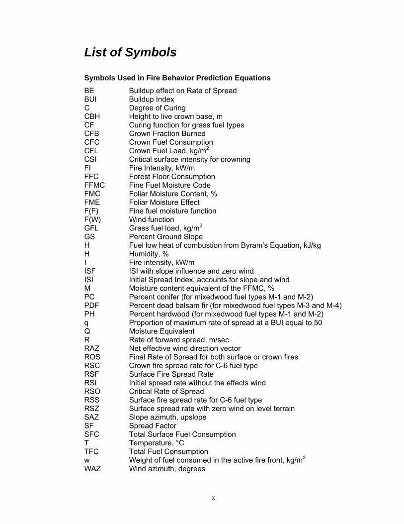
List of Symbols Symbols Used in Fire Behavior Prediction Equations BE Buildup effect on Rate of Spread BUI Buildup Index C Degree of Curing CBH Height to live crown base, m CF Curing function for grass fuel types CFB Crown Fraction Burned CFC Crown Fuel Consumption CFL Crown Fuel Load, kg/m2 CSI Critical surface intensity for crowning FI Fire Intensity, kW/m FFC Forest Floor Consumption FFMC Fine Fuel Moisture Code FMC Foliar Moisture Content, % FME Foliar Moisture Effect F(F) Fine fuel moisture function F(W) Wind function GFL Grass fuel load, kg/m2 GS Percent Ground Slope H Fuel low heat of combustion from Byram’s Equation, kJ/kg H Humidity, % I Fire intensity, kW/m ISF ISI with slope influence and zero wind ISI Initial Spread Index, accounts for slope and wind M Moisture content equivalent of the FFMC, % PC Percent conifer (for mixedwood fuel types M-1 and M-2) PDF Percent dead balsam fir (for mixedwood fuel types M-3 and M-4) PH Percent hardwood (for mixedwood fuel types M-1 and M-2) q Proportion of maximum rate of spread at a BUI equal to 50 Q Moisture Equivalent R Rate of forward spread, m/sec RAZ Net effective wind direction vector ROS Final Rate of Spread for both surface or crown fires RSC Crown fire spread rate for C-6 fuel type RSF Surface Fire Spread Rate RSI Initial spread rate without the effects wind RSO Critical Rate of Spread RSS Surface fire spread rate for C-6 fuel type RSZ Surface spread rate with zero wind on level terrain SAZ Slope azimuth, upslope SF Spread Factor SFC Total Surface Fuel Consumption T Temperature, °C TFC Total Fuel Consumption w Weight of fuel consumed in the active fire front, kg/m2 WAZ Wind azimuth, degrees

xi

WFC Woody Fuel Consumption WS Observed wind speed, km/h WSE Slope equivalent wind speed WSV Net wind speed vector WSX Net wind speed vector in the x direction WSY Net wind speed vector in the y direction Symbols Used in Developing the CWSPM α Direction angle between the directions being considered for fire

spread and the direction from which the frictions are acting. k Varies directional dependency of the DISPERSE function

1

Chapter 1: Introduction

1.1 Background

Created by natural or man-made activities, it is estimated that wildfires around

the globe burn over 750,000 square kilometers of forest each year

(Rothermel, 1993). Canada’s forests alone comprise ten percent of the

world’s forests and feed an annual average of 9,500 wildfires burning roughly

three million hectares. These fires can be devastating for both the

environment and the economy. Currently, fifty-six percent of Canada’s forests

are commercially productive and contribute upwards of fifty billion dollars to

the national economy each year. On the other hand, the financial loss caused

by forest fires average around one billion dollars annually. As a specific

example, Canada’s boreal forest fires in 2000 took a devastating toll on the

environment and resulted in one-billion dollars of lost revenue (State of

Canada’s Forests, 2000).

There are many causes of wildfires. Many fires are started unintentionally or

carelessly. However, the two most frequent natural causes of wildfires are

lighting and the friction of wind rubbing dry wood together. The most frequent

unnatural causes include campfires, discarded cigarettes, controlled burning,

equipment fires, railroad sparks and juvenile stupidity (State of Canada’s

Forests, 2000).

1.1.1 Benefits and Drawbacks of Wildfires

In some instances wildfires can provide benefits to the forest ecology by

burning away dead, decaying debris and initiating new growth. On the other

hand, uncontrolled wildfires can be devastating and result in irreversible

changes to the environment.

2

1.1.1.1 Benefits of Wildfires

When managed properly, wildfires clear away the dead, decaying vegetation

that accumulates on the forest floor. This promotes new growth and reduces

the possibility of potentially larger, more disastrous, uncontrolled fires. In

addition, for some tree species, fire is the only way to reproduce. The intense

heat of a fire opens the pinecones that protect the tree’s seeds. These seeds

can take root in the area of the passing fire or can be transported by the

strong, turbulent winds from the fire to be planted tens or hundreds of meters

away (Rothermel, 1993). Another advantage of wildfires is that they break

down organic mater into soil nutrients. In many cases, landscapes once

devastated by fire are bursting with new, healthy growth within a few years.

1.1.1.2 Disadvantages of Wildfires

Wildfires can also be devastating by degrading the environment and

diminishing natural resources. The burning of tropical forests alone pumps

2.4 gigatonnes of carbon into the atmosphere per year (Rothermel, 1993).

This translates to thirty percent of the total carbon dioxide emissions in the

world. Wildfires can also kill wildlife, create mudslides/landslides as a result

of the absent vegetation, reduce the aesthetics of the environment, threaten

families and homes and influence long-term health problems as a result of the

increased air pollution.

1.1.2 Potential Fire Hazards for Today’s Forests

How to best preserve the world’s forests has been a topic of debate since the

late 1970’s. Before the extensive fire suppression efforts that began thirty

years ago, small-scale fires swept through landscapes every five to twenty-

five years (Gayton, 1998). However, since the seventies, fire suppression

technology has greatly improved and wildfires occurring near communities are

not tolerated as a natural phenomenon. Decades of successful fire

suppression activity have allowed many forests to grow uninfluenced by fire.

3

As a result of this, it is not uncommon for some forests to become ingrown

and slowly suffocate themselves to death (Parsons, 1978; Gayton, 1998).

The amount of dead vegetation in these forests put them at risk of feeding

huge fires that could consume valuable lumber resources, devour fire

suppression budgets, and threaten the safety of both fire-fighters and nearby

communities.

As a result of these increasingly more common, high impact fires it is

important to develop accurate fire modeling techniques that can predict fire

danger and spread. Accurate fire modeling will give fire management crews

more time to prepare fire breaks to help gain control of large fires in addition

to providing insight on ways to improve the best possible techniques of

suppressing fires of any size.

1.2 Methodology

The background on fire research that was conducted for this thesis involved

extensive reading and personal interviews. From the advice of Cordy

Tymstra, Fire Science and Technology Supervisor with Alberta Sustainable

Resource Development (SRD), three courses were taken by the author to

gain the knowledge needed to write this thesis. The first course entitled

“Principles of Fire Behavior” (Principles of Fire Behavior, 1993) described the

accepted theories of how environmental parameters affect fire behavior. All

wildland firefighters working in Alberta must take and pass this course to be

granted employment. The focus of the next two courses was on the two

completed components of the Canadian Forest Fire Danger Rating System

(CFFDRS). One course discussed the general equations of the Fire Behavior

Prediction System (Hirsch, K. G., 1998) and the other course described the

general equations of the Fire Weather Index System (Understanding the Fire

Weather Index System, CD). These systems will be discussed in more detail

in the body of the thesis. It is the theories of fire behavior that are presented

in these courses that are stated in this thesis. Altering opinions by academia

are not explored.

4

From the information gained on the background reading that was undertaken

and interviews with Cordy Tymstra from the SRD office in Edmonton, Alberta

and Rick Arthur from the SRD office in Calgary, Alberta, it was learned that

there are three main problems in the wildfire management and monitoring

industry.

The first problem is that currently Alberta has no prescribed fire policy. This

creates inconsistencies between different fire management districts in the

province. The second problem is that each fire management district is using

different programs for their management systems. This creates sub-optimal

communication between different agencies and inconsistent criteria for fire

prediction. The third problem is that the current data acquisition system could

be improved to include higher accuracy hot spot detection within existing fires.

This research set out to provide solutions to the first problem by investigating

the existing Canadian and Albertan policy to identify what is stated about

prescribed burning and to locate gaps in the policy. The author made contact

with Morgan Kehr who is the Prescribed Fire Operational Coordinator for

Alberta SRD and was informed that no documents had yet been drafted to

identify the information that should be included in the new Albertan policy. In

order to continue the research, existing American prescribed burning policy

was investigated to determine how the subject of prescribed burning is

approached. Merits and shortcomings of American prescribed fire policy and

relevant portions of Canadian fire policy were identified and recommendations

were made to the new Albertan prescribed fire policy.

To solve the two remaining problems the author was introduced to two

different fire management systems; one used by the SRD department in

Edmonton and one used by the department in Calgary. At a subsequent

interview with Cordy Tymstra, the author was told that having a unified fire

management system to link the different fire management districts in Alberta

would be a very beneficial tool to the future development of the wildfire

industry. It was decided by the author and after the advice of the author’s

supervisor to develop an Internet based wildfire management system to

5

accomplish this task. Further research on the requirements of a wildfire

management system determined that the most necessary component was a

wildfire prediction model. Research on existing models revealed that

Canadian prediction modeling software could be improved. It was then

decided to build a fire behavior prediction model that overcame some of the

shortcomings of the existing models.

Development of the Canadian Wildfire Spread Probability Model (CWSPM)

and criteria development for the Web based management system began in

January of 2003. To save time, a website programmer was used to

implement the requested criteria into the website. The criterion for the

website was to implement the following:

• Implement the Data Acquisition System developed by the Mobile Multi-

Sensor Systems research group at the University of Calgary (Wright,

2004) for real-time forest fire hotspots detection.

• Add a database containing information on past Albertan fires.

• Include a distance to nearest lake tool to allow fire managers to easily

locate the nearest water resources.

• Include a flight trajectory tool to show the observatory path that spotter

aircrafts have taken.

• Include the CWSPM as the fire behavior prediction model.

The CWSPM was designed as a probability model that used standard

Canadian fuel type data that is accepted by the CFFDRS. The model was

developed to have input based on a scheme of weighted parameters. The

values for the weighted parameters were chosen by a trial and error method

that linked the weighted parameters as closely as possible to the results of the

CFFDRS. This will be discussed in more detail in Chapter 4. By spring of

2003 a new model called the Prometheus model was developed by Alberta

Sustainable Resource Development. This model is to become the Canadian

standard for fire modeling. Even though the CWSPM was being developed it

6

was decided by the author to use the Prometheus model in the website in

place of the CWSPM. This choice was made for the following reasons.

• The new Prometheus model has a Microsoft Component Object Model

that allows it to be easily programmed into a website.

• The WMMS system will gain more recognition because it is using

Prometheus.

• The Prometheus model uses the equations of the CFFDRS

• Prometheus is to become the standard model across Canada.

• The University of Calgary could work with SRD to debug the

Prometheus COM which SRD plans to implement into their own future,

Internet based, wildfire management system.

Despite the choice to use the Prometheus model in the development of the

Web based wildfire management and modeling system, development of the

CWSPM was still completed. The intention of the CWSPM shifted from being

used as the web based fire modeling system to being a Canadian model that

fire managers or the general public could use to get quick, easy to compute,

predictions of fire spread probabilities.

1.3 Problem Statement

There are three problems that need to be addressed to improve the efficiency

of the wildfire industry. Solutions to these problems will greatly improve

communications and make wildfire management more efficient. The three

problems are:

1. Wildfire policy does not adequately outline guidelines that should be

followed when conducting prescribed burns

2. Canadian fire modeling programs are sub optimal and should be improved

3. Communications between fire management districts are sub optimal and

should be improved with the introduction of an Internet based wildfire

management and modeling system.

7

1.4 Research Objectives

The main objective of this research is to find ways to improve the existing

practices of managing and modeling wildfires by finding solutions to the three

wildfire management problems previously stated. This is accomplished in this

thesis by breaking the main objective down into four sub-objectives.

The first sub-objective is to investigate the parameters that influence fire

behavior to learn how wildfires react to various elements in the environment.

The second sub-objective is to identify fire policy and find the inadequacies so

that recommendations can be made to the new Albertan prescribed fire policy.

This would solve the first problem existing in wildfire management. The third

sub-objective is to investigate benefits and short comings of existing fire

models. Finding ways to improve existing models will help determine the

requirements needed in a new fire model. This would solve the second

problem existing in wildfire management. The fourth sub-objective is to

develop a new fire modeling and management system. This includes the

development of the new CWSPM and the development of the web based

wildfire management and modeling system. It is anticipated that this research

will inspire fire managers to reassess the way that wildfires are managed and

promote the development of a more robust, complete fire management and

modeling. This last sub-objective would offer one solution to the third problem

existing in wildfire management.

1.5 Thesis Outline

This thesis is divided into six chapters. The following section breaks down the

contents of each remaining chapter.

Chapter 2 will give background information on the importance of wildfire

modeling. This chapter will,

8

• give an overview of the parameters that affect fire spread

• discus the different techniques used in fire monitoring

• discuss the gaps in Albertan prescribed fire policy and make

recommendations for future policies

Chapter 3 will discuss in detail the procedures and mathematical equations

used by Canadian Fire Managers to predict rate of fire spread and fire

intensity. In addition, it will analyze the existing software for performing fire

growth predictions and will discuss how the models can be improved.

Chapter 4 will use the information discussed in the first three chapters to

discus the design and development of the CWSPM. This model will be

compared to the actual final fire perimeter of a historic fire. The intent of

developing this model was to design a Canadian fire prediction model that

surpassed the functionality of existing models. This model was to be

integrated into the Web based wildfire modeling and management system that

was designed by the author but instead the recently developed Prometheus

fire behavior prediction model is used. The development of the CWSPM is

included in this thesis to demonstrate a valuable tool for quick, easy to

compute, fire probability predictions.

Chapter 5 will discuss the functionality of an Internet based, real time, Wildfire

Modeling and Management System (WMMS), which is the apex of this thesis’

research. In this chapter the reader will discover the abilities of the system,

how it was developed and how it can be utilized to revolutionize wildfire

modeling. This system combines one of the most advanced hotspot detection

systems available to date with the most advanced fire behavior prediction

model in Canada to create a real time Internet based GIS that could change

the way wildfires are managed in Canada.

The WMMS integrates the following features into a real-time data updating

system and GIS based web browser:

9

• Real time airborne thermal infrared and RGB images of current fires

• Real time spotter aircraft flight trajectories

• Active fires reported by management or the general public

• Fire history of each fire management district

• Fire behavior predictions for future fire spread based on algorithms

used by the fire behavior prediction software Prometheus (designed by

the Alberta Government in 2003)

This system has the potential to greatly improve fire management’s abilities to

monitor this natural disaster and can be utilized by both fire managers and the

general public. It has the potential to have a significant impact on how

wildfires are combated resulting in reduced damage to the environment,

improved safety of fire crews and appreciable financial savings.

Communication techniques between the different facets of fire management

personnel also have the potential to improve as this system harnesses some

unique ways of displaying data and monitoring fire behavior (Trevis and El-

Sheimy, 2004). Some possible improvements to the system and future work

will also be discussed.

Chapter 6 will give the final conclusions and recommendations for this

research.

Some of the material presented in Chapter 5 has been previously published in

papers. In those cases where the candidate has been the author or a co-

author of these papers, quotations are not indicated as such, but are simply

referenced.

10

Chapter 2: Background to Fire Modeling

2.1 Parameters that Affect the Behavior of Wildfires

Wildfire behavior is dictated by the elements present in the surrounding

environment. There are three broad factors that contribute to the behavior of

wildfires. They are (Principles of Fire Behavior, 1993):

1. Fuel

2. Topography

3. Weather

2.1.1 Fuel

Fuel affects fire behavior in a number of ways. The most obvious way is by

the type of fuel the fire consumes. Fuel is described as any type of vegetation

that can be consumed by a fire. Different types of vegetation will burn at

different rates due to their size, shape, compactness, horizontal and vertical

continuity, moisture content and chemical composition (Urban-Wild Land

Interface Fire: The I-Zone Series).

Fuel size affects how easily new fires can be started by spotting. Spotting

occurs when burning fuels are lifted up into the air by the upward drafts of the

fire’s convection currents and dropped outside the fire line to start new fires

(Brown, 1973). These convection currents are created by cold air that is

sucked into the fire and forced upwards as the air heats up from the fire.

Debris can be carried by these convection currents distances of a few meters

to hundreds of meters depending on the strength of the convection currents

and the weight and shape of the debris. Small embers can easily be lifted up

by the fire’s convection currents but cannot maintain long-term combustion.

This prevents most small embers from starting long-range spot fires and

allows them to ignite fires only a short distance from the main fire. In addition,

11

small embers may not be able to generate enough heat to ignite some

vegetation types. Larger embers, on the other hand, have the size needed to

provide enough heat to ignite unburned vegetation, provided the convection

currents are strong enough to lift them into the air.

The shape of the fuel also influences its ability to spread or sustain a fire.

Round embers can contribute to fire behavior because they have the ability to

roll down existing slopes and create new fires in unburned fuels in the valleys

below. Flatness and surface area of a burning fuel also influence its ability to

start new fires. As the flatness and surface area to volume ratio increases it

becomes easier for convection currents to pick up embers and carry them

longer distances. These more aerodynamic embers are able to start new fires

sometimes hundreds of meters way from the original fire line (Principles of

Fire Behavior, 1993).

Fuel compactness will also affect fire behavior. Loosely compacted fuels will

allow more complete combustion thereby accelerating the spread of the fire.

On the other hand, tightly compacted fuels will slow down combustion, slow

down the fires rate of spread but increase the fire’s intensity (Brown, 1973).

Horizontal and vertical continuity of fuels also influence how easy it is for a fire

to gain intensity. Fuels that lack horizontal continuity can make a fire loose

momentum and put itself out (Carmody, 2001). Similarly, fuels that lack

vertical continuity discourage the vertical extent of the fire and hinder the fires

progression from surface fires to more intense crown fires.

The moisture content of fuels also greatly affects fire behavior. Moist fuels will

be hard to burn because the water in the fuel absorbs the majority of the initial

heat. This will hinder fire growth. In comparison, dry fuels act like kindling for

the fire and provide extra heat and flame that will help ignite the moister fuels.

The increased moisture content in leaves when compared to coniferous tree

needles is one reason why fires in deciduous forests are on average less

numerous and less violent than fires in coniferous forests (Johnson, 2001).

12

Chemical content of fuels also influences fire behavior. Some saps, resins

and pitch are flammable and can greatly accelerate or intensify the spread of

fire. On the other hand cow pies and moist duff act as fire retardants and

hamper the rate of spread (Principles of Fire Behavior, 1993).

2.1.1.1 Fuel Type Acting as a Barrier to Fire Spread

When looking at the behavior of wildfire propagation there are a number of

parameters that act as natural barriers to fire growth (Principles of Fire

Behavior, 1993). Rock, paved roads and bare soil act as unburnable barriers

to fire and can halt a fire from crossing over these surfaces. This will, of

course, depend on the width and length of the barrier since fires can easily

burn around and over small obstacles. If a fire is large enough to spot across

a rock or bare soil barrier then the obstacle is not impermeable and will only

aid in slowing down the fire’s rate of spread. Trails and cut lines also impede

the growth of fires. Heavily traveled trails will act as a bare soil barrier and cut

lines change the vegetation type from trees to grasses. This fuel type change

could take a crown fire down to a surface grass fire. Any change in fuel type

can have such an effect on the behavior of wildfires. Depending on the fuel

type change the fire could either accelerate or be slowed. Recently burned

vegetation also acts as a natural fire barrier by not having much unburned fuel

to ignite. Lakes and streams also act as barriers in two ways. The first way is

that it is impossible for water to burn so the fire must stop at the lake or

riverbank or have enough intensity to jump the river and burn the opposite

bank. The second way is that vegetation on the banks of lakes and rivers

usually have a higher moisture content, which will make the vegetation harder

to ignite. This in itself will aid to slow the fire.

2.1.2 Topography

Topography plays an important role in fire behavior. It can be described by

three sub-parameters.

13

• Slope

• Aspect

• Elevation

Slope affects fire behavior in a number of ways. First, the steeper the slope

the faster the fires rate of spread upslope (Brown, 1973). This is due to the

higher degree of fuel preheating caused by the smaller angle between the

ground and flames. In addition, if there is a great deal of solar radiation on

the slope during the day, wind will be created during the night as the land

cools and a nighttime inversion develops. This wind can push the fire down

slope in unexpected directions. The specific shape of the terrain also affects

fire behavior. Ridges can slow a fire because they hinder the preheating of

fuels on the other side of the ridge whereas chutes running up the sides of

mountains can rapidly speed up the spread of fire by creating steep slopes on

three sides of the fire and promoting spread in three different directions.

Saddle slopes can be particularly dangerous since fire behavior and spread

direction becomes unpredictable, as there are both upward slopes and ridges

in the same area. In this case the fire can spread up one slope, up the other,

or up both. Areas such as saddle slopes are also often the locations where

fire whirls will develop (Principles of Fire Behavior, 1993). Fire whirls or

vortexes are comparable to dust devils or even tornadoes but comprised of

both wind and fire instead of just wind. These phenomena can accelerate

away from the core of the fire leaving trails of fire behind them. They are

particularly dangerous both for their unpredictable nature in combination with

the high speed of the winds that make them. It has been found that wind

speeds in the center of a fire whirl can exceed one-hundred and sixty

kilometers per hour. They eventually dissipate as they leave the convection

currents and heat of the main fire.

Slopes can also provide shelter for small fires and allow them to grow without

being put out by the wind. In this manner, shelter can also allow spotted

embers to ignite new vegetation and start a new fire. Local weather patterns

can also be affected by slope (Principles of Fire Behavior, 1993).

14

Aspect affects fire behavior because of the different local climates on slopes

facing different directions. North of the equator, south facing slopes will

generally be dryer than north facing slopes because they receive more solar

radiation (Brown, 1973). This means that there is more potential for a fire to

burn on south facing slopes. South facing slopes also promote fire spread by

having higher average temperatures.

Elevation is also an influential factor for fire spread. Like aspect, elevation

influences the moisture content of fuels. It is indirectly related to curing

densities, temperature, snowmelt dates and precipitation (Principles of Fire

Behavior, 1993).

2.1.3 Weather

Weather is the most variable and influential component for fire spread.

Weather affects temperature, fuel moisture, wind speed and atmospheric

stability which all play a role in fire behavior. Temperature is important

because the hotter the fuel is, the less preheating needed to ignite it. Fuel

moisture, which has already been discussed in the previous section, is related

to precipitation and humidity. As the precipitation in a certain area increase,

the moisture content in the fuels will also increase and igniting the vegetation

will become more difficult.

Wind is perhaps the most influential component of weather when dealing with

fire behavior. Wind does many things to influence the propagation speed and

direction of an active fire. Wind has the ability to dry fuels thusly making them

more susceptible to fire. It also supplies oxygen to feed the fire and can bend

fire flames to be more parallel to the ground thereby helping them ignite new

vegetation (Principles of Fire Behavior, 1993). A fire can seem unaffected by

near zero wind velocities or, in the case of high winds, follow the direction and

speed of the wind without any apparent regard for any other parameters such

as fuel or topography. Winds such as the Chinook winds of Alberta, Canada

15

are particularly dangerous since they are strong, hot, dry winds that can

greatly accelerate the spread of fire (Hirsch, 1998). Fire managers must be

very aware of the wind speed and direction because it can vary greatly from

hour to hour or even minute to minute. If the wind direction changes suddenly

the fire crew could become trapped by the fire or have the fire begin racing

towards them. This is why weather observations are so important for fire

management and modeling.

Atmospheric stability is also a contributor to fire behavior (Principles of Fire

Behavior, 1993). There are two types of atmospheres that one must be

aware of when dealing with wildfires: stable and unstable atmospheres.

Stable atmospheres occur when there is an inversion and warmer air rises to

rest on top of cooler air that is closer to the ground. In this case, air

temperature will increase with increased height above the ground. Unstable

atmospheres occur when warmer air is closer to the ground and cooler air

rests above. In this case air temperature will decrease with increasing height.

These two conditions can affect a fire’s size and intensity. Stable

atmospheres will restrict the vertical development of convection currents and

in turn slow growth and intensity. This is because the hot air created from the

fire will be unable to rise above the warm air that is in the higher levels of the

atmosphere. This prevents strong updrafts that encourage higher fire

intensities and long range spotting. Stable atmospheres will also promote

milder and steady winds. Unstable atmospheres on the other hand,

encourage the vertical development of large convection currents, which will

increase the growth, and intensity of the fire. This is because, in unstable

atmospheres, the hot air created by the fire is able to rise to incredible heights

and this creates strong updrafts and compensating downdrafts. Under these

conditions, large wildfires can often create their own local weather patterns

which can include local thunderstorms and gusty winds. These winds are

particularly hard to incorporate into wildfire models, due to their

unpredictability, and have a large influence on fire spread. They also have

the capability of uprooting fully grown trees and displacing them outside the

most actively burning part of the fire (Brown, 1973).

16

Cloud cover also indirectly influences fire behavior. Clouds affect the degree

of solar radiation that is received by the fuels and can hinder preheating and

drying of the fuels (Urban-Wild Land Interface Fire: The I-Zone Series).

2.2 Detecting Wildfires

Today, look-out stations, airborne remote sensing and public sightings are the

most common methods used to detect forest fires. In the province of Alberta,

Canada, forty percent of all wildfires are detected by sightings from fire

lookout stations, twenty percent from aerial sightings and forty percent from

public sightings (Wildfire Detection, 2004).

Much research has been conducted on satellite aided wildfire detection,

monitoring and modeling. Remote Sensing’s ability to cover large areas in a

single image makes it an option for wildfire detection and modeling (Sannier,

2002). Some satellites of choice for this procedure are images from the

Advanced Very High Resolution Radiometer (AVHRR) aboard the National

Oceanic and Atmospheric Administration (NOAA) series satellites or

Moderate Resolution Imaging Spectrometer (MODIS) images. Detection of

wildfires using these methods has proven to be successful however; there are

a number of drawbacks that do not allow it to be used for high accuracy

monitoring or modeling. The first drawback is that the resolutions of many of

the satellite images suitable for wildfire detection are very coarse (i.e. NOAA

AVHRR has a pixel resolution of 1.1 Km at nadir (Fernandez, 1997)). This

means that fires must burn to a considerable size before the satellites can

detect them. In addition, it is impossible to differentiate between a single fire

and a group of smaller fires (Mahmud, 1999, Knapp, 1996). Predicting the

exact perimeter or where the fire is likely to propagate in the future is

therefore impossible. Satellites with higher resolution such as IKONOS are

possibilities but these have no thermal capabilities to detect the heat of the

fire or identify hot spots and obtaining the images is too expensive to have

any practical use for this application. The second drawback is that many

images taken by these satellites have extensive cloud cover that conceals the

17

evidence of existing wildfires (Mahmud, 1999). Since a single satellite image

does not have the spatial resolution, real time capabilities or spectral range

needed for high accuracy management and modeling (Knapp, 1996), they will

not be discussed further. The application that does have this capability is

photogrammetry, which will be discussed next.

Aerial photogrammetry is a common method used to monitor forest fires and it

solves many of the problems that occur when using satellite images for this

application. To use photogrammetry, a camera is mounted on the bottom of a

spotter aircraft and, in combination with GPS positioning and inertial

navigation systems, the physical properties and GPS locations of the fire can

be determined as the aircraft passes over the area of interest. The images

acquired by photogrammetry depend on the type of camera that is used.

Video, visual RGB or thermal cameras can be used together or separately to

obtain the desired type of information.

One advantage of photogrammetry is that it can be viewed in three

dimensions if two images contain the same point of interest. If two such

photos exist, these images can be viewed in stereo. A second advantage of

photogrammetry is that the resolution of the images can be controlled (within

reason) depending upon the flying height of the spotter aircraft (El-Sheimy,

2000). A third advantage of photogrammetry is that the images can be taken

when required. One does not have to wait for the satellite’s next pass over

the area. A fourth advantage of photogrammetry is that the images are taken

below the elevation of the clouds; therefore, there are fewer obstructions on

the image. Smoke from the fire will still cause obstructions in the images for

the visual RGB cameras but thermal cameras are insensitive to smoke and

the heat signatures of the fire can still be clearly identified.

18

Methods used for detecting hotspots and monitoring wildfires are very

important to ensure that the fires are detected in the most efficient and cost

effective method available.

2.3 Resources Used to Combat Fire

There are many resources used to combat wildfires. These resources include

bulldozers to make firebreaks, water/fire-retardant bomber aircrafts and

people with hoses, pick axes and shovels doing what they can to douse the

fire or create firebreaks. One controversial method of combating fire is by

starting new, smaller, controllable fires in the line of the main fire. Setting fires

removes the fuel that is needed to feed the main fire and can effectively

redirect or halt the advancing fire front (Clugston 2003). Purposely setting a

fire with the intention of helping forest health or managing an existing wildfire

is called prescribed burning. Although controversial, extensive prescribed

burns are what some fire managers believe is the only solution to prevent

these large-scale wildfires that have run rampant in many of Canada’s forests.

To find a solution to the first problem in wildfire management that this thesis is

trying to solve, the next section will investigate prescribed burning and related

policy. It will pinpoint the weaknesses in Canadian policy and make

recommendations for future policies.

2.3.1 Prescribed Burning

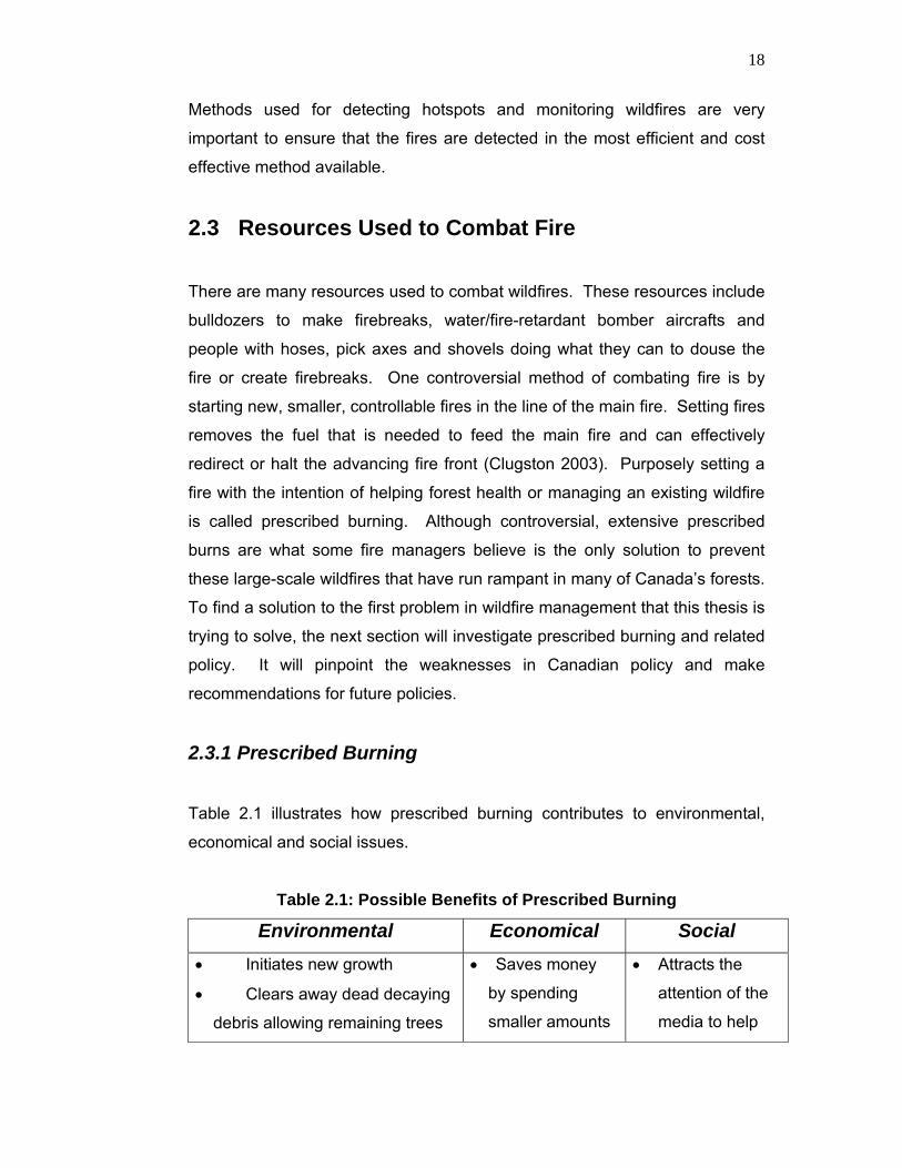
Table 2.1 illustrates how prescribed burning contributes to environmental,

economical and social issues.

Table 2.1: Possible Benefits of Prescribed Burning

Environmental Economical Social • Initiates new growth

• Clears away dead decaying

debris allowing remaining trees

• Saves money

by spending

smaller amounts

• Attracts the

attention of the

media to help

19

to have better access to the sun

(Gayton, 1998)

• Replenishes the soil with

nutrients

• Reduces ignition potential

• Mitigates the potential for

future extreme fires to occur in

the area (Gayton, 1998)

• Controls insect infestation

and disease (Denison, 1997)

• Increases water yield for

remaining vegetation (Parsons,

1978)

• Helps some tree

species(i.e. jack pine) that need

fire to regenerate or the trees

will die (Jack Pine Ecosystem,

2003)

• Helps maintain the habitat

of some animal species such as

the Kirtland warbler who are

dependant on the large

branches of young jack pine

forests (Jack Pine Ecosystem,

2003)

of the budget to

control small

prescribed fires

and not having to

fight expensive,

extreme fires

• More

economical than

mechanically

thinning the trees

(Denison, 1997)

• Saves

residential

housing in the

case of a larger

fire

inform citizens

of the hazards

of large

amounts of fuel

build up and

how to better

protect their

homes from fire

(Koehler, 1997)

• Produces less

smoke and ash

than the

potentially more

extreme fires

that could

sweep through

the landscape if

no action is

taken

Table 2.1 clearly indicates that there are a number of positive environmental,

economic and social aspects outlining how prescribed burning aids forests.

Despite these sound arguments, there are some arguments that state that

prescribed burning is not a solution to forest management. These arguments

are stated in the Table 2.2 below:

20

Table 2.2: Possible Negative Impacts of Prescribed Burning

Environmental Economic Social • Causes smoke and ash

• Releases carbon into

the atmosphere

• Allows the possibility for

a fire to escape and

become a large fire

(Gayton, 1998)

• Lacks proof of

effectiveness until an un-

prescribed fire sweeps

through the landscape.

• Causes skepticism of

spending money on a

fire if you do not have

to

• Offers no guarantee

that a prescribed burn

will save money in the

future

• Creates high liabilities if

personal property is

damaged or destroyed

• Causes smoke

and ash which

could lead to

temporary health

ailments

• Creates public

skepticism

regarding any

forest fire

The main difference between the two schools of thought is that the arguments

stating that prescribed burning is not sustainable are intangible and

hypothetical “what ifs”, whereas the arguments stating that prescribed burning

aids forest sustainability are often more tangible and documented from the

state of our current forests and results of historical fires.

The advantage of prescribed fires is that they are intensely monitored and

only preformed on days where the wind and humidity provide conditions that

are adverse to extreme fire behavior. The ferocity of prescribed fires can also

be controlled to administer the type of fire that would be most advantageous

to a specific forest. Surface fires could be used to control dead vegetation

and debris on the forest floor, more intense crown fires could be used to open

pinecones and start new forests. Prescribed burning is also favorable to

mechanical thinning since the process is less expensive and some of the

tree’s nutrients are recycled back into the ground. With mechanical thinning

these nutrients are removed along with the trees.

21

2.3.1.1 Prescribed Burning and Policy

Canada has no federal fire policy but instead allows the provinces to develop

their own policies. Currently, within each province a limited practice of

prescribed burning is used to help forest sustainability. Surprisingly, in the

province of Alberta, Canada there is no existing policy that outlines a set of

standardized criteria that need to be followed before a prescribed burn can be

administered (Kehr, 2004). This task is left up to the manager of each Wildfire

Management Area. The policy that exists today, The Forest Protection Policy

Manual and Standard Operating Procedures, only states that prescribe

burning can be used as a tool for sustainable forest management (Forest

Protection policy Manual & Standard Operating Procedures, 2003). No

indication of where or when prescribed burning is allowed is outlined in this

policy. To remedy this, Morgan Kehr from Alberta Sustainable Development

is heading a team who is currently writing an Alberta Prescribed Fire Policy

that will outline the standardized criteria for prescribed burns in Alberta (Kehr,

2004). The details of this policy are not yet available.

A policy specifically meant for prescribed burning is important because there

are significant differences between general wildfires and prescribed burns.

There are at least nine items that should be dealt with in a prescribed burn

policy that are not needed in a wildfire policy. These items are listed below:

1. Descriptions of the methods used to ignite prescribe fires and defined

guidelines for choosing the safest ignition method

2. Goals intended by having the prescribed fire

3. Identified ideal and unacceptable weather condition criteria

4. Descriptions of the minimum amount of needed suppression/monitoring

forces

5. Weighting systems for risks based on certain weather, topography and

fuel type combinations to create a “go”/”no go” criteria for the

prescribed burn

6. Pre-created backup plans in case prescribed fires escape

22

7. Environmental impact assessments

8. Economic advantage of using prescribed burning instead of other

forest thinning techniques

9. Procedures to determine what type of fire will be the most beneficial for

a certain type of forest

Since Alberta has no prescribed fire policy, the United States federal

prescribed fire policy will be used to analyze how policy attempts to outline the

use of prescribed fires. Recommendations can then be made for Alberta’s

new policy based on the merits and shortcomings of the American policy. The

criteria stated in the American Wildland Prescribed Fire Management Policy

include developing a burn plan that specifies the:

• desired fire effects,

• weather conditions that will promote acceptable fire behavior,

• forces needed to ignite, hold, monitor, and extinguish the fire and

• level of risk (low, medium or high) if the burn is conducted

(Zimmerman, 1998)

If a prescribed burn is calculated as a high risk then the burn will not be

permitted. A go/no-go checklist must also be completed before the burn can

be conducted.

Environmental Policy

There is one major problem with the American federal prescribed fire policy

that the Alberta government should consider when designing a policy of their

own. Strict environmental policies have made it very difficult to meet the

criteria needed to perform a prescribed burn and often no burns are permitted

because of this. Despite the pressure from environmentalists, President

George W. Bush and the US Congress needed to pass the “Healthy Forest

Initiative” in 2003, which allows more relaxed restrictions regarding the use of

prescribed burning and forest thinning (Healthy Forests, 2002). This initiative

23

no longer restricts the size of trees that can be burned or cut to improve

overall forest health and allows more funding for prescribed burns that follow

the existing policy. Environmentalists disagree with this initiative because

they believe that not enough forests near residences were included in the

project and also believe that the project may contain a loophole which will

allow an increase in commercial logging (Doering, 2003). This complaint

seems unrealistic as fifty percent of the budget for this project is reserved for

forests near residential areas. It is true that this initiative may bring more

profit to loggers but the existing funds for prescribed burning were too limited

and, using Washington, Oregon and California’s forests as an example, not

adequate enough to effectively promote sustainable forest health.

In Alberta’s case, care should be taken to insure that environmental policies

meld with the Albertan Prescribed Fire Policy. This may take some pro active

effort in developing public awareness to inform the population of the benefits

of prescribed burning and how it promotes forest sustainability. Also, ingrown

forests near residences should be made a higher priority for burning than

remote forests. It would be beneficial for the forest manages to work in a

partnership with the insurance companies to initiate programs to identify the

potential problem areas and deal with them accordingly.

Economic Policy

An insertion of the economic advantages or disadvantages of a prescribed

burn should also be included in Alberta’s new prescribed fire policy. Although

it is expected that some cost/benefit analysis be done before prescribed

burning is performed, these requirements were not stated in any of the

policies that were looked at. A portion of policy should be reserved for

addressing the economic topics relating to forest sustainability that were

outlined in Tables 2.1 and 2.2.

24

Health and Safety Policies

The issue of health and safety is very significant when discussing prescribed

burning and forest sustainability, since the fires are purposely set. Prescribed

burning, in many cases, is both environmentally and economically

sustainable; however, this operation must also be considered socially

beneficial to be a good technique for improving forest health. A major

concern is air pollution caused by prescribed burns. Environmentalists and

some members of the general public argue that prescribed burns should not

be allowed because they release unnecessary carbon dioxide and ash into

the air. Alberta again has no prescribed burning policy and therefore initiates

no health or safety standards for this matter. One important recommendation

for Alberta, which is currently mandatory in the Unites States, is to only

administer a prescribed burn if it can be predicted that the degradation of air

quality in any nearby community is still within the guidelines of any clean air

policy such as the Clean Air Act (Super, 2002). Before prescribed burns can

be conducted in the United States, environmental assessments must be

preformed to ensure that the amount of smoke particles in the air will be less

than the air quality standards set by the Environment Protection Agency

(Glickman, 1995). If the predicted winds or size of the fire have the potential

to lower the air quality of nearby residences below the standard, the burn is

not permitted.

The other safety policies that are in Alberta’s Standard Operating Procedures

are relevant enough to ensure that fire-fighter safety is a top priority. Perhaps

one of the most important existing policy inclusions is the right for a worker to

refuse work if they feel they are in “imminent danger” (Super, 2002). Also in

Alberta, mandatory safety briefings are held for all crew members each day.

As another precaution, a Safety Officer is assigned to every fire and reports

on any problems, issues, concerns during the fire and makes

recommendations on how safety could be improved for the next wildfire

suppression activity.

25

2.3.1.2 Effectiveness of Policy

If Alberta adopts many of the recommendations outlined in this section,

prescribed burning could prove to be an effective tool to maintain forest

sustainability for issues of environmental, economical and social importance.

The only remaining precaution will be to ascertain the effectiveness of the

new policy. In the past, the only area where prescribed burning has become

an unsustainable tool is when control of the prescribed fire is lost. The

following list is a set of three different escaped prescribe burns that have

happened in the United States and the damage they caused.

• Cerro-Grand Fire, New Mexico - burned 235 residences in Los Alamos

(Cerro Grande Prescribed Fire, 2000)

• Lowden Ranch, California – burned 23 residences (Lowden Ranch

Prescribed Fire Review, 1999)

• Sawtooth Mountain, Arizona – 1 Fatality (Sawtooth Mountain

Prescribed Fire Burnover Fatality, 2003)

In these three cases, and in most prescribed burn runaways, not following the

guidelines of the existing policy was the cause of the loss of control of the fire

(Sawtooth Mountain Prescribed Fire Burnover Fatality, 2003; Cerro Grande

Prescribed Fire, 2000; Lowden Ranch Prescribed Fire Review, 1999; Conroy,

2003). The reasons for the failure of these three example cases are stated

below:

Cerro Grand Fire:

• Pertinent weather information was not collected;

• Did not follow the burn plan procedure that was approved by the state.

Lowden Ranch Fire:

• The required number of crew were not present at the burn site;

• Three of the four men in charge were not adequately briefed and had

not reviewed the burn plan.

26

Sawtooth Mountain Fire:

• Prescribed burn was unapproved;

• Burn preformed in temperatures that were too high and humidity that

was too low;

• Killed worker did not follow the safety standards by:

failing to follow the burn plan;

working alone.

In each of these cases, if the policy had been followed these disasters would

probably have been avoided. A quote from the U.S Department of the

Interior, Bureau of Land Management who oversees the Fire Incident Reports

states:

“When agencies do fail, it is generally not because of a lack of

adequate policy, standards and guidance, but a result of not

following that guidance. Agencies write a plan, but do not live

the plan (Lowden Ranch Prescribed Fire Review, 1999).”

There are a number of different ways that policy is reviewed in Canada and

the United States. As mentioned earlier, in Alberta, a Safety Officer is

assigned to every fire. It is then the safety officer’s responsibility to enforce

existing policy and to recommend ways that policy can be improved.

Problems arising from using prescribed burning as a tool for sustainable

development do not lay in the method or in policy but in human error. It is a

proven fact that forests need fires to regenerate and our intense fire

suppression activities have not helped sustain our forests but rather helped

them slowly suffocate and die. The use of prescribed burning has the

potential to improve forest health from an economic viewpoint while producing

minimal adverse effects. Prescribed burns will also reduce the future chance

that large, uncontrollable fires will ignite in the area.

27

2.4 Summary This chapter discussed the following,

• Parameters affecting forest fire behavior;

• Methods used to detect fires;

• Methods used to combat fires;

• Policy weaknesses in regards to wildfire management and

recommendations on what should be included in future Albertan policy.

Currently wildfire policy does not outline guidelines that should be followed

when conducting prescribed burns. This chapter has provided a solution to

this first problem facing wildfire management. The creation of a new Albertan

policy for prescribed burning that follows the recommendations in this chapter

will help to ensure that prescribed burns are carried out safely and effectively.

The next chapter discusses how to mathematically predict fire spread and

introduces some of the fire models that are used in Canada and the United

States. Chapter 3 supplies the background information that is needed to

solve the second problem regarding suboptimal Canadian fire behavior

modeling.

28

Chapter 3: Fire Prediction and Modeling

3.1 Predicting Fire Behavior

The first attempt at predicting fire spread using a mathematical approach was

achieved by W. R. Fons in 1946 (Rothermel, 1972). He focused on the head

of the fire and concluded that a fire spread by employing a series of

successive ignitions of the fine fuels in the landscape. A certain amount of

heat was needed to ignite these fine fuels and fire spread depended on the

time period between ignitions and the distance between the particles in the

fine fuels.

Since then, two schools of thought have developed in North America and

have become the standards that are used when determining how to predict

the spread of wildfires in Canada and the United States. Forest fire managers

in the United States use equations developed by Richard C. Rothermel in

1972 (Rothermel, 1972). Canadians use equations based on the Fire

Intensity Equation developed by Byram in 1956 (Forestry Canada Fire Danger

Group, 1992).

3.1.1 The Rothermel Model

In 1972 Richard C. Rothermel, who worked as a Research Engineer at the

Northern Forest Fire Laboratory in Missoula, Montana, developed a

mathematical model for fire propagation (Rothermel, 1972). This model

attempted to integrate all the variables in the fire environment (Bachmann,

2000). It was unique in the fact that it was able to model the relationship

between the burning fire front and the energy released to the adjacent fuels

(Urban-Wild Land Interface Fire: The I-Zone Series). No other model was

able to do this before. Many wildfire models used today employ algorithms

that were designed by Rothermel. This model uses seventeen input variables

that describe fuel types, moisture content, slope, aspect and wind patterns

29

(Rothermel, 1972). Since this model is used primarily in the United States the

equations that make up the model will not be discussed. For extensive detail

about this model and the equations that complete it refer to Rothermel, 1972.

3.1.2 Byram’s Fire Intensity Equation

The mathematical model that Canada uses to predict the rate of spread and

fire intensity of wildland fires is inspired by Byram’s Fire Intensity Equation,

I H w R= (1)

Where,

I is the fire intensity measured in kW/m.

H is the fuel low heat of combustion measured in kJ/kg.

w is the weight of fuel consumed per unit area in the active fire

front measured in kg/m2.

R is the rate of forward spread in m/sec (Forestry Canada Fire

Danger Group, 1992).

In the ten years after its development, this equation gained widespread

acceptance by Canadian fire managers and researchers. Accordingly, it was

decided in the mid 1960’s to use a version of Byram’s Fire Intensity Equation

for Canadian forest fire predictions. As a result, the Canadian Forest Fire

Danger Rating System (CFFDRS) was developed to implement this equation.

3.1.3 Predicting Fire Spread Using the Methods of the CFFDRS

The CFFDRS is currently the Canadian standard for predicting wildfires and

was initially developed in 1968 (Hirsh, 1996). To enable it to predict fire

behavior using Byram’s fire intensity equation, two sub-systems have been

developed to handle the fuel type, topography and weather input parameters.

The two sub-systems that have been developed are called the Fire Behavior

Prediction System (FBP) and the Fire Weather Index (FWI) System. They are

used to calculate the predicted values for w and R in Byram’s Equation. A

30

third sub-system is currently being developed to include risk of lightning and

human caused fires.

The FBP system uses fuel types and topography to calculate quantitative

predictions for select characteristics of fire behavior (Hirsh, 1996). Fuel types

across Canada have been grouped into sixteen standard classes to help

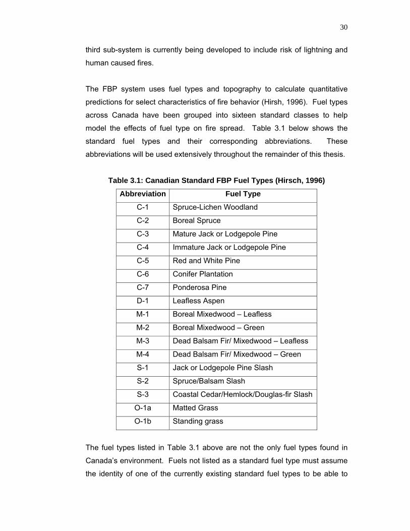
model the effects of fuel type on fire spread. Table 3.1 below shows the

standard fuel types and their corresponding abbreviations. These

abbreviations will be used extensively throughout the remainder of this thesis.

Table 3.1: Canadian Standard FBP Fuel Types (Hirsch, 1996)

Abbreviation Fuel Type

C-1 Spruce-Lichen Woodland

C-2 Boreal Spruce

C-3 Mature Jack or Lodgepole Pine

C-4 Immature Jack or Lodgepole Pine

C-5 Red and White Pine

C-6 Conifer Plantation

C-7 Ponderosa Pine

D-1 Leafless Aspen

M-1 Boreal Mixedwood – Leafless

M-2 Boreal Mixedwood – Green

M-3 Dead Balsam Fir/ Mixedwood – Leafless

M-4 Dead Balsam Fir/ Mixedwood – Green

S-1 Jack or Lodgepole Pine Slash

S-2 Spruce/Balsam Slash

S-3 Coastal Cedar/Hemlock/Douglas-fir Slash

O-1a Matted Grass

O-1b Standing grass

The fuel types listed in Table 3.1 above are not the only fuel types found in

Canada’s environment. Fuels not listed as a standard fuel type must assume

the identity of one of the currently existing standard fuel types to be able to

31

utilize the FBP calculations. The restricted number of available fuel types is a

limitation of the system. An example of problems encountered when using

limited fuel types arises when wildfires spread through un-modeled

agricultural crops. In situations such as this the FBP system may not produce

optimal results.

The FWI system is composed of six components that model fire behavior

based on fuel moisture and wind dynamics. The first three components deal

with the moisture content of fuels on the forest floor. The layers are defined

as scattered litter and other fine fuels, loosely compacted organic layers at

moderate depth and deep, compacted layers. The three remaining

components of the FWI system include predicted rate of fire spread, fuel

available for combustion and predicted head fire intensity. These six

components are calculated using the equations from Van Wagner, 1987.

The CFFDRS method of predicting fire intensity differs from Byram’s equation

in a number of ways. First, Byram’s equation is meant to use observed input

values as parameters in the equation. When using the CFFDRS method, only

predicted values are available. Second, the value for H has been changed

from a variable into a constant value of 18,000 kJ/kg. This value is the

average heat of combustion for the sixteen fuel types outlined in the FBP

system. The value of 18,000 was chosen based on results of measurements

taken from small scale fires occurring in various fuel types. The CFFDRS

version of Byram’s Fire Intensity Equation can now be shown. The resulting

equation is Equation 2 below:

ROSTFCFI ××= 18000 (2)

Where,

FI is the fire intensity measured in kW/m.

TFC is the predicted total fuel consumption measured in

kg/m2.

ROS is the predicted Rate of Spread measured in m/min.

32

An extensive number of equations must be computed before the intensity of a

fire can be calculated. The next few pages will illustrate the background for

these equations. All equations have been taken from Forestry Canada Fire

Danger Group, 1992 unless otherwise stated.

3.1.3.1 Calculating Fine Fuel Moisture Code and Buildup Index

The first set of equations that need to be calculated when determining a fire’s

Rate of Spread and Fire Intensity are the Surface Fuel Consumption (SFC)

equations. To solve the equations for Surface Fuel Consumption, the Fine

Fuel Moisture Code (FFMC) and Buildup Index (BUI) must be calculated.

Fine Fuel Moisture Code

The FFMC describes the moisture content of the upper most layer of fuel on

the forest floor. This upper most layer is called the surface litter layer and is

approximately 1.2 centimeters in depth (Understanding the FWI, CD). This

parameter may change hourly and certainly daily and is greatly dependant on

temperature (T - in degrees Celsius); humidity (H - in percent); wind speed (W

- in kilometers per hour) and rainfall (r0 - in millimeters). FFMC values can

influence the likelihood and speed of surface fire spread, spotting probability

and extreme fire behavior. The FFMC is related to ease of ignition because

the upper most layer of the forest floor is where most fires ignite. For the

FFMC equation and derivation refer to Van Wagner, 1987.

If the FFMC calculations produce values below seventy-four it is unlikely that

a fire will be able to ignite in that location (Understanding the FWI, CD). This

is because the fuel moisture content is too high to support combustion.

Values greater than ninety-two indicate that there is the potential for extreme

fire behavior.

33

Buildup Index

The BUI models the amount of fuel available for burning. It is calculated using

two input variables concerning the moisture of the fuels in the two lower layers

of the forest floor, namely the Duff Moisture Code and the Drought Code. The

Duff Moisture Code (DMC) represents the moisture of the fuel in the forest

floor layer that is just below the fine fuel litter layer. Fuels available for

burning in the DMC layer are located up to a depth of about seven

centimeters under the surface litter layer. The DC represents the Drought

Code and corresponds to the moisture of the fuel in the deep layers of the

forest floor. These layers reach an approximate depth of about eighteen

centimeters (Understanding the FWI, CD).

Calculating the Duff Moisture Code for the BUI

The first BUI parameter that will be discussed is the DMC. The DMC is

important for fire modeling because this layer of the forest floor is where the

fire front gains most of its energy. DMC is influenced by daily temperature,

relative humidity and rainfall. The equation for the DMC (Van Wagner, 1987)

was calculated based on four years of empirical observations of the duff layer

in red pine and jack pine forest stands in the 1970’s. Based on the same

observations it was discovered that when the DMC of a duff layer reaches

values higher than forty it is able to contribute to Fire Intensity and fire Rate of

Spread. At values lower than twenty this layer will not ignite or be involved in

the burning of forest fuels (Understanding the FWI, CD). This is because the

moisture content of the duff layer is too high for combustion to be able to

occur.

Calculating the Drought Code

The second parameter needed for the BUI calculation is the Drought Code.

This code is an indicator of smoldering combustion, seasonal drought and

total fuel consumption. It is affected by the daily rainfall, noon temperature

and month of year (Understanding the FWI, CD). If the value of the DC is

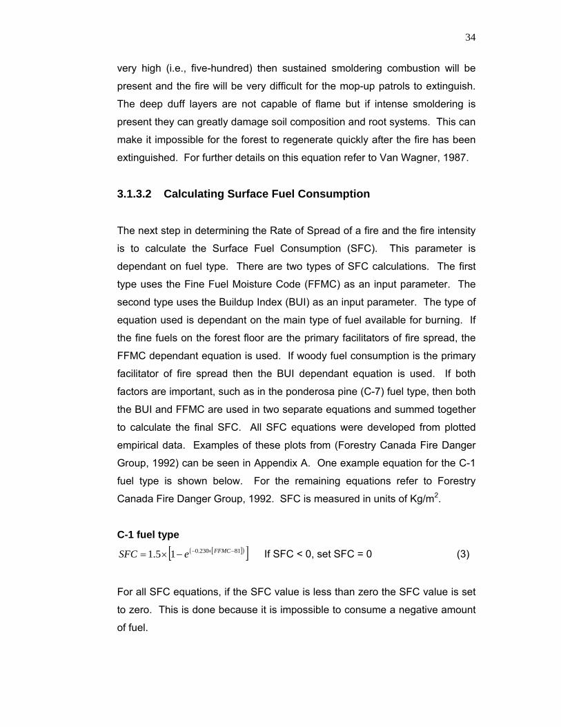
34

very high (i.e., five-hundred) then sustained smoldering combustion will be

present and the fire will be very difficult for the mop-up patrols to extinguish.

The deep duff layers are not capable of flame but if intense smoldering is

present they can greatly damage soil composition and root systems. This can

make it impossible for the forest to regenerate quickly after the fire has been

extinguished. For further details on this equation refer to Van Wagner, 1987.

3.1.3.2 Calculating Surface Fuel Consumption

The next step in determining the Rate of Spread of a fire and the fire intensity

is to calculate the Surface Fuel Consumption (SFC). This parameter is

dependant on fuel type. There are two types of SFC calculations. The first

type uses the Fine Fuel Moisture Code (FFMC) as an input parameter. The

second type uses the Buildup Index (BUI) as an input parameter. The type of

equation used is dependant on the main type of fuel available for burning. If

the fine fuels on the forest floor are the primary facilitators of fire spread, the

FFMC dependant equation is used. If woody fuel consumption is the primary

facilitator of fire spread then the BUI dependant equation is used. If both

factors are important, such as in the ponderosa pine (C-7) fuel type, then both

the BUI and FFMC are used in two separate equations and summed together

to calculate the final SFC. All SFC equations were developed from plotted

empirical data. Examples of these plots from (Forestry Canada Fire Danger

Group, 1992) can be seen in Appendix A. One example equation for the C-1

fuel type is shown below. For the remaining equations refer to Forestry

Canada Fire Danger Group, 1992. SFC is measured in units of Kg/m2.

C-1 fuel type [ ]( )[ ]81230.015.1 −×−−×= FFMCeSFC If SFC < 0, set SFC = 0 (3)

For all SFC equations, if the SFC value is less than zero the SFC value is set

to zero. This is done because it is impossible to consume a negative amount

of fuel.

35

A constant value is used to calculate the SFC for the grass fuel type. This

constant value was chosen since there is no organic fine fuel layer in grass

fuel types and it is assumed that all the grass is consumed during the

passage of the fire front so there is no need to compute a Buildup Index. The

SFC for grass is then equal to the grass fuel load (GFL), which has a standard

value of 0.3 kg/m2 (Forestry Canada Fire Danger Group, 1992).

3.1.3.3 Computing Initial Rate of Spread

The next step in fire modeling is to compute the Initial Rate of Spread (RSI).

The RSI can be described as the rate of spread of a fire through level terrain

under equilibrium conditions (Forestry Canada Fire Danger Group, 1992).

Equilibrium conditions mean that the fire is no longer accelerating its burning

pattern from a point source fire but that the fire front can be treated as a line

fire acting independently from the initial point where the fire ignited. Similarly

to surface fuel consumption, the RSI is dependant on fuel type and has

therefore been divided into equations (Forestry Canada Fire Danger Group,

1992) that vary slightly depending on the input fuel type. Just as in the

equations used for Surface Fuel Consumption the RSI equations have been

developed from best fit curves of plotted empirical data. For the examples of

these curves please refer to Appendix B. An example equation for RSI that

applies to many of the fuel types is shown below. For the equations and

details for the remaining fuel types refer to Forestry Canada Fire Danger

Group, 1992.

C-1 to C-7, M-3, M-4, S-1 to S-3 and D-1 fuel types

( )[ ]cISIbeaRSI ×−−×= 1 (4)

The constants, a, b and c, are Rate of Spread constants and can be obtained

from (Forestry Canada Fire Danger Group, 1992). The ISI parameter

indicates the Initial Spread Index parameter. This variable indicates the

speed that a fire will spread across a terrain with no regard for fuel type.

36

Grassy fuel types use a different form of equation to calculate Initial Rate of

Spread. When looking at fire spread through grasslands it becomes apparent

that the degree of curing (C) is very important when determining grass fire

spread rates. Curing is described as the percent of grass steams that have

dried and are no longer green (Forestry Canada Fire Danger Group, 1992).

To incorporate the degree of curing into a rate of spread equation the

percentage of curing is turned into a curing coefficient. There was no

empirical data to create this equation so Forestry Canada designed this

equation to be linear where the fire has no potential to spread if the degree of

curing is less than fifty percent. If this occurs CF equals zero. This is done

because it is assumed that a grass stand will not burn if green grass makes

up at least fifty percent of the stand (Understanding the FWI, CD). It was also

desired to keep the curing coefficient values between zero and one. The

graph from which this equation was derived is shown in Figure 3.1 below.

Figure 3.1: Relationship between CF and Degree of Curing for Grass Fuel Types

(Van Wagner, 1987)

The equation for Curing Coefficient is shown in Equation 5.

0.102.0 −×= CCF C > 50 (5)

CF represents the Curing Coefficient and C is the degree of curing recorded

in percent.

37

The adjusted Final Rate of Spread equation for grass is then the Initial Rate of

Spread Equation shown in Equation 4 multiplied by the Curing Coefficient.

The equation is shown below,

( )[ ] CFeaROS cISIb ×−×= ×−1 (6)

Where a, b and c are the rate of spread constants from (Forestry Canada Fire

Danger Group, 1992). To view the rate of spread plots that were used to

derive Equation 6 please refer to Appendix B. The plots for standing and

matted grass have been derived from empirical data collected on grass fires

in Australia (Forestry Canada Fire Danger Group, 1992).

3.1.3.4 Calculating Final Surface Rate of Spread

To calculate the Final Rate of Spread, slope must be taken into consideration.

One example method of calculating slope is shown below. This equation

uses elevation rise divided by horizontal ground distance.

100tan__

_×=

ceDisGroundHorizontalRiseElevationGS (7)

Where, GS is the slope of the ground measured in percent.

The Spread Factor (SF) due to slope was calculated from empirical

observations of fire behavior on various slopes. It describes how quickly a fire

will spread depending on the degree slope of the terrain and is the next

parameter that must be identified. The graph is shown below.

38

Figure 3.1: Relationship between the Spread Factor and Percent Slope

(Forestry Canada Fire Danger Group 1992)

Equation 8 is the equation of the curve depicted in Figure 3.2. It can be used

to compute SF as shown below.

2.1

100533.3 ⎟

⎠⎞

⎜⎝⎛×

=GS

eSF (8)

Forestry Canada does not recommend that Equation 8 be used for slopes

greater than sixty degrees. This is because the SF increases drastically for

slopes greater than sixty degrees and, due to lack of empirical evidence, it is

uncertain if Equation 8 remains true for these steep slopes (Forestry Canada

Fire Danger Group, 1992).

Using Equation 9 below the Slope Adjusted Zero Wind Rate of Spread (RSF)

can be computed. This equation represents the effect of slope on the rate of

spread assuming that no wind is present. The SF and a variable called the

Zero Wind Rate of Spread (RSZ) are used to compute the RSF parameter.

SFRSZRSF ×= (9)

Where the RSZ is calculated using a variation of the appropriate RSI

equation, whose example is shown in Equation 4. The difference between the

RSZ and RSI equations is that the RSZ equation uses different parameters to

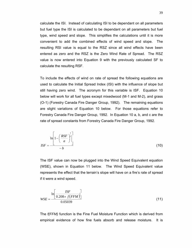
39

calculate the ISI. Instead of calculating ISI to be dependant on all parameters

but fuel type the ISI is calculated to be dependant on all parameters but fuel

type, wind speed and slope. This simplifies the calculations until it is more

convenient to add the combined effects of wind speed and slope. The

resulting RSI value is equal to the RSZ since all wind effects have been

entered as zero and the RSZ is the Zero Wind Rate of Spread. The RSZ

value is now entered into Equation 9 with the previously calculated SF to

calculate the resulting RSF.

To include the effects of wind on rate of spread the following equations are

used to calculate the Initial Spread Index (ISI) with the influence of slope but

still having zero wind. The acronym for this variable is ISF. Equation 10

below will work for all fuel types except mixedwood (M-1 and M-2), and grass

(O-1) (Forestry Canada Fire Danger Group, 1992). The remaining equations

are slight variations of Equation 10 below. For those equations refer to

Forestry Canada Fire Danger Group, 1992. In Equation 10 a, b, and c are the

rate of spread constants from Forestry Canada Fire Danger Group, 1992.

b

aRSF

ISF

c

−

⎥⎥

⎦

⎤

⎢⎢

⎣

⎡⎟⎠⎞

⎜⎝⎛−

=

1

1ln

(10)

The ISF value can now be plugged into the Wind Speed Equivalent equation

(WSE), shown in Equation 11 below. The Wind Speed Equivalent value

represents the effect that the terrain’s slope will have on a fire’s rate of spread

if it were a wind speed.

( )05039.0

208.0ln ⎥

⎦

⎤⎢⎣

⎡×

=FFMf

ISF

WSE (11)

The f(FFM) function is the Fine Fuel Moisture Function which is derived from

empirical evidence of how fine fuels absorb and release moisture. It is

40

dependant on the FFMC value discussed earlier. Details about this

parameter can be found in Van Wagner, 1987.

Now, the Wind Speed Equivalent (WSE) and the actual wind speed (WS)

must be combined to attain the total effect of both parameters. Vector algebra

is used to preserve both the magnitude and direction of the force of the wind.

( )[ ] ( )[ ]SAZWSEWAZWSWSX sinsin ×+×= (12)

( )[ ] ( )[ ]SAZWSEWAZWSWSY coscos ×+×= (13)

22 WSYWSXWSV += (14)

⎟⎠⎞

⎜⎝⎛= −

WSVWSYRAZ 1cos (15)

Where WSX is the magnitude of the resulting force in the x direction and WSY

is the magnitude of the resulting force in the y direction. WAZ and SAZ are

the Wind Azimuth Direction and Uphill Slope Azimuth Direction respectively.

WSV is the Net Effective Wind Speed and RAZ is the Net Effective Wind

Direction (Forestry Canada Fire Danger Group, 1992).

From this point the WSV is used for all remaining computations involving wind

speed. The RAZ is used as the fire spread direction when growing fire

perimeters on GIS models as discussed in the next chapter.

The Initial Spread Index value which includes the effects of wind speed can

now be calculated. See Van Wagner, 1987 and Forestry Canada Fire Danger

Group, 1992 for the full description of the equation. Two forms of this

equation exist. The first version is used for wind speeds less than or equal to

forty kilometers per hour. In the case of very intense wind speeds (values

above forty kilometers per hour) an adjusted wind function parameter in the

ISI equation must be used (Forestry Canada Fire Danger Group, 1992).

The next step in the Canadian fire modeling procedure is to calculate the

Buildup Effect (BE). This parameter is a function of the BUI discussed earlier.

41

Its purpose is to give the Initial Spread Index a parameter that accounts for

the fuel available for combustion that is not as variable and dependant on fuel

moisture as the BUI. The BE has been developed to equal zero when the BUI

equals zero and levels off at extreme BUI values. This inverse relationship is

accomplished by subtracting the average BUI, BUI0, from the inverse of the

calculated BUI for that fuel type. A value, q, was also introduced to help

determine the value of the BE. The value of q will increase or decrease

depending on how the increasing depth in the forest floor of each fuel type will

influence a fire’s rate of spread. The value q represents the proportion of the

maximum possible spread rate, without regard for the ISI, determined from a

standard BUI value of fifty (Forestry Canada Fire Danger Group, 1992). This

constant of fifty was chosen because it was the average BUI calculated for all

fires contained within the CFFDRS database. The resulting equation for BE is

shown below,

( )⎥⎥⎦

⎤

⎢⎢⎣

⎡⎟⎟⎠

⎞⎜⎜⎝

⎛−××

= 0

11ln50BUIBUI

q

eBE (16)

The BUI0 and q values are constants and can be obtained from Forestry

Canada Fire Danger Group, 1992.

The BE can now be used with the RSI (whose example calculation is shown

in Equation 4) to determine the Final Rate of Spread, ROS, measured in

meters per minute.

BERSIROS ×= (17)

Equation 17 will not work for the conifer plantation fuel type. Additional

information is needed to determine the Final Rate of Spread for this

parameter. Reasons for this and the Rate of Spread calculations for the C-6

fuel type will be discussed after the calculations for Crown Fire Rate of

Spread.

42

3.1.3.5 Calculating Crown Fire Rate of Spread

For all coniferous forest fuel types, crown fuel involvement can be quite

influential on Fire Intensity and Rate of Spread. To identify when an initial

surface fire will gain enough intensity to involve the tree crowns, the Critical

Surface Fire Intensity (CSI) equation must be calculated. This equation

depends on Crown Base Height (CBH) and the Foliar Moisture Content

(FMC).

Calculating Foliar Moisture Content

The Foliar Moisture Content (FMC) describes the amount of moisture content

in needles of conifers that are at least one year old. It is an important

parameter for coniferous forests because it affects the initiation of crowning

and the rate of crown fire spread (Forestry Canada Fire Danger Group, 1992).

This parameter varies with location and time of year. The FMC can be

calculated in two different ways depending on what initial information is

available. Both methods have been derived based on six years of empirical

data. One method is used if only latitude and longitude information on the site

is available. The second method is used if information on latitude, longitude

and elevation of the site are available. For these equations refer to Forestry

Canada Fire Danger Group, 1992.

Once the FMC has been determined it can be used in the Critical Surface Fire

Intensity (CSI) equation shown below.

( ) 5.15.1 9.25460001.0 FMCCBHCSI ×+××= (18)

The Crown Base Height, CBH, is previously calculated from empirical data

and is used as a constant. The values for the CBH for each fuel type can be

found in Forestry Canada Fire Danger Group, 1992.

43

The CSI is used to determine the Critical Surface Fire Spread Rate (RSO). If

the Rate of Spread, ROS, is larger than the Critical Surface Fire Spread Rate,

RSO, the tree crowns will become involved in the fire and the ROS value must

be adjusted to account for this. If the surface fire Rate of Spread exceeds the

Critical Surface Fire Spread Rate by ten meters per minute it is assumed that

the tree crowns are at least ninety percent involved in the fire (Forestry

Canada Fire Danger Group, 1992). This equation is derived from Byram’s

Fire Intensity Equation shown in Equation 2.

SFCCSIRSO×

=300

(19)

If the ROS computed in Equation 19 exceeds the RSO and crown

involvement is assumed, the crown fraction burned (CFB) can be computed

using the following equation,

( )RSOROSeCFB −×−−= 23.01 (20)

3.1.3.6 Rate of Spread for Coniferous Plantations

The Final Rate of Spread for the coniferous plantation is treated differently

from any other fuel type because these plantations tend to be more uniform

than most natural forest stands and therefore have a different influence on fire

behavior. Because of their structure, this fuel type is more easily modeled

when separated into surface and crown fire rates of spread. One of the

parameters needed to compute the Rate of Spread for the C-6 fuel type is

different than the parameters used for the other fuel types and will be

discussed here. This parameter is called the Foliar Moisture Effect (FME). It

is an adjusted version of the FMC that accounts for the increased spacing

between the trees of the coniferous plantation fuel type. This increased

spacing allows for more oxygen to access the fire and aids more complete

combustion and higher fire intensities. It is assumed that the oxygen supply is

doubled in C-6 stands (Forestry Canada Fire Danger Group, 1992). The FME

equation is found in Forestry Canada Fire Danger Group, 1992.

44

And the Crown Fire Spread Rate is,

( )avg

ISI

FMEFMEeRSC ×−×= ×− 0.10497.0160 (21)

Where the average FME (FMEavg) is equal to 0.778 and is chosen by

empirical methods (Forestry Canada Fire Danger Group, 1992).

Now, using the RSI from example Equation 4 and the BE from Equation 16

the Surface Fire Spread Rate is,

(22)

The equation for the Final Rate of Spread in a coniferous plantation fuel type

is shown in Equation 23.

)( RSSRSCCFBRSSROS −×+= (23)

Where

RSS is the Surfaced Fire Spread Rate in m/min

CFB is the Crown Fraction Burned

RSC is the Crown Fire Spread Rate in m/min

3.1.3.7 Calculation of Fire Intensity

To calculate Fire Intensity the Total Fuel Consumption (TFC) must be

computed first. The equation to compute Total Fuel Consumption is

comprised of variables for the Surface Fuel Consumption (SFC) and the

Crown Fuel Consumption (CFC). The Surface Fuel Consumption equation

has already been described in example Equation 3. The Crown Fuel

Consumption Equation can be computed by multiplying the Crown Fuel Load

(CFL) by the Crown Fraction Burned (CFB).

BERSIRSS ×=

45

CFBCFLCFC ×= (24)

Where CFL a constant found in Forestry Canada Fire Danger Group, 1992.

The Total Fuel Consumption is the result of a simple addition between the

Crown Fuel Consumption and the Surface Fuel Consumption.

CFCSFCTFC += (25)

Finally, Fire Intensity can be calculated using the variation of Byram’s Fire

Intensity Equation from Equation 2.

ROSTFCFI ××= 18000

TFC is the Surface Fuel Consumption (SFC) in the case of the S, D and O

class fuel types or the TFC in the case of coniferous forest fuel types. The

Fire Intensity is calculated in units of kW/m.

There are many steps that are employed to calculate the final Rate of Spread

and Fire Intensity of a wildfire. This process is very tedious but very

necessary when trying to predict wildfire propagation. Regardless of the

mathematical model used, there are three reasons why the results of the

mathematical model may not parallel what is observed in reality (Urban-Wild

Land Interface Fire: The I-Zone Series). These reasons include:

1. Model not applicable to the fire scenario

2. Model has errors inherent in its design

3. Data used in the model is either too generalized, not accurate or out of

date

Many fire modeling software programs have been developed in Canada and

the United States. Most Canadian models use equations from the CFFDRS

just described; however, there are some other sets of equations such as

Rothermel’s equations which are used for many American models. Different

46

models use different methods for displaying their information and use different

parameters depending upon the country or specific site they were developed

for. Some of the techniques used to design these models and an overview of

the more popular models will be discussed next.

3.2 Background to Existing Fire Prediction Models 3.2.1 Spatial vs. Non-spatial Models

In the realm of fire propagation models there are two categories that models

can be placed in regarding the way that they display their results: spatial

models and non-spatial models. Spatial models allow the user to see a

pictorial representation of how the fire is propagating through the terrain.

Non-spatial models do not give pictorial representations but rather display the

fire propagation information in the form of graphs and charts.

Each model has a number of advantages and disadvantages. Non-spatial

models are easier to develop and require less sophisticated computer

hardware to display the results. They are however, less intuitive and more

cumbersome to use because they require the interpretation of numerical

values. Spatial models on the other hand require less interpretation and the

user can visualize the predicted fire propagation patterns on the computer

screen in the form of an image. The drawback of spatial models is that they

require more computer memory and are more difficult to develop. In addition

to the mathematical equations used to calculate a fire’s rate of spread and

intensity, a spatial model requires a method of representing how these

parameters can be accurately displayed on the computer screen. There are

two different base techniques that can be employed to do this when designing

spatial models. The two techniques are The Cellular (Point) Propagation

Technique and The Wave (Vector, Curve) Propagation Technique (Tymstra,

1999). These techniques will be discussed in the next sections.

47

3.2.2 Fire Propagation Techniques for Spatial Models

3.2.2.1 The Cellular Technique

The Cellular or Point Propagation Technique is a common method used in fire

growth models (Tymstra, 1999). This technique uses raster grids of regular

cells both as data input layers and as the template for propagating the fire. If

a cell is determined to be a “fire” cell, then, the fire from that cell is able to

propagate to any of the eight neighboring cells in the next iteration.

Successive fire predictions are then performed on the neighboring cell that

has the soonest arrival time.

There are two major drawbacks associated with the Cellular Propagation

Technique. The first is that fires in reality do not naturally propagate in

patterns of regular grids. Because of this regular gird and restricted possible

fire spread direction, the predicted size and shape of fires are often unrealistic

when using the Cellular Model (Finney, 1998). The second drawback is that

this model struggles when neighboring cells are not homogeneous. When

encountering cells with different wind speeds, wind directions or fuel types the

accuracy of the model diminishes (Finney, 1998). The Wave Propagation

Technique attempts to resolve these inefficiencies.

3.2.2.2 The Wave Technique

The concept of Wave Propagation was initially developed by Dutch

mathematician, Christian Huygens in 1678 to explain the behavior of traveling

light waves (Finney, 1997). In 1975 Gywn Richards from Brandon University

adopted this principle to describe fire growth behavior (Urban-Wild Land

Interface Fire: The I-Zone Series). He analytically derived a differential

equation that determines a fire’s propagation from a single point. This theory

is actualized in fire modeling by defining a fire ignition point or perimeter using

a vertex or vertices. Each vertex is given x and y coordinates. Expansion of

the fire perimeter is then determined by calculating the Rate of Spread (ROS)

48

and zero-wind-slope direction vector (RSF) using the equations discussed in

the previous section. Time is introduced into the model by multiplying the

Rate of Spread by a chosen time-step. Since the ROS equation is only useful

for the head fire spread rate, a fire shape must be introduced to determine the

spread rate in the directions other than exactly perpendicular to the fire

perimeter. Ellipses are the most common and widely accepted shape used

when trying to mimic a fire’s spread. However, ellipses are not the only

relevant shapes as shown by the research done by Byram in 1959 on fan

shapes (Finney, 1998) and by Richards in 1990 on lemniscate shapes

(Finney, 1998). For the purposes of this research only the most common

shape, the ellipse, will be discussed. To spread the fire from each vertex

along the fire perimeter an ellipse is drawn in an orientation coincident with

the no-wind-slope direction vector. The vertex is often situated on the rear

end of the semi major axis as shown in diagram A of Figure 3.3. In the case

of no-wind, a circle is drawn with the vertex located at the center of the circle.

The ratio between the semi minor and semi major axis of the ellipse is

dependant on the fire behavior parameters of that vertex. As each time step

is completed the fire polygon will enlarge, the number of vertices will increase

and new ellipses will be computed for the subsequent iterations (Finney,

1998).

The new fire perimeter is then determined by adding new vertices at the head

of each ellipse and joining the vertices together by a line. This is the method

shown in Figure 3.3, Diagram B. The second method uses the boundaries of

the ellipses as the new fire perimeters. If the ellipses calculated for two

neighboring vertices overlap, the overlapping boarders are dissolved and the

resulting irregular shape takes the place of the two ellipses. New vertices are

then created along the new perimeter and the process is repeated for the next

time step. This process is performed for all ellipses around the fire perimeter.

49

Figure 3.2: Diagrams of the Elliptical Fire Growth Technique (Finney, 1998)

Diagram A in Figure 3.3 above depicts the elliptical fire spread under uniform

conditions. There is a small constant effective wind in this diagram, which

accounts for the slightly elongated ellipse. Diagram B depicts the elliptical fire

spread under non-uniform conditions of both fuel type and effective wind

speed. From this diagram it can be seen how the fire perimeter can become

irregular.

The Wave Propagation Technique avoids some of the problems encountered

when using the Cellular Propagation Technique. Problems such as geometric

distortion, under estimation of size and incorrect location of fire perimeters are

reduced with the use of this second model (Finney, 1998). This model also

has faster computational speeds. The drawback of this technique is that the

coding is more in depth.

Now that the basic elements of fire propagation models have been discussed

this chapter will delve into analyzing the positives and negatives of the

different fire propagation models that are currently available. The section

below does not give a complete list of all the possible fire models but rather

discusses the models that are most commonly utilized within Canada and the

United States.

50

3.3 Evaluation of Existing Fire Propagation Models

The purpose of investigating existing fire models is to determine what features

should be included in a new model that will be implemented on an Internet

based wildfire management and modeling site. Six models will be

investigated in this section.

3.3.1 BehavePlus Version 2.0 The first model that will be discussed is called BehavePlus which replaces its

prior edition named BEHAVE. BEHAVE was developed in the early 1980’s by

the U.S. Forest Service (Grabner, 1999). This model is a non-spatial model

whose output is displayed through the use of graphs, charts and simple

diagrams. The system was designed to be both a fire modeling tool and a

learning guide for new fire management trainees. BehavePlus and

accompanying tutorials are available for download, free of charge, at:

http://fire.org.

BehavePlus has many abilities as a fire modeling tool. A basic, but very

important, ability is that it is able to run on most IBM compatible machines. As

for its modeling abilities, it uses wind speed and direction, percent slope, fuel

moisture content and fuel model number as input variables. The first three

parameters are self explanatory however, the last parameter, the fuel model

number, describes the fuel type used by the surface fire spread model. The

fuel model number is the American version of the sixteen standard fuel types

that Canadians use. BehavePlus has thirteen different fuel models that can

be used to approximate the vegetation type of a particular landscape. All

input variables are used in equations outlined by Rothermel’s Model

described earlier. (As each fire model is explored in this section it will become

increasingly apparent that many models use the algorithms proposed by

Rothermel.) Using these input parameters and the Rothermel model,

BehavePlus is able to output the following parameters (Hunter, 2004):

51

• Surface fire rate-of-spread and intensity

• Heat per unit area

• Safety zone size

• Size of a point source fire

• Fire containment

• Spotting distance

• Crown scorch height

• Tree mortality

Despite the abundance of information this model provides, there are a number

of limitations that hinder its success. The first is that this model is capable of

modeling only surface fires. Fires of a larger intensity, such as crown fires,

cannot be modeled using this program. The second limitation is that the fuel

type is assumed to be continuous, uniform, homogeneous and contiguous to

the surface. This means that variations in the ground cover are not taken into

consideration. The third limitation is that the conditions of the fire environment

are assumed to be constant. This includes slope, aspect and weather

parameters which are simplified into uniform constants. Simplifying these

three parameters could greatly affect the results of the model. The wind

condition would be especially affected since wind speed and direction can

change so rapidly and have such a large effect on fire behavior. The fourth

and final limitation is that the model does not have spatial capabilities so the

output parameters must be interpreted from various tables. This is perhaps

the most important limitation since it is very difficult to relate a numerical value

of rate of spread to actual area covered on the ground on all sides of the fire

front.

3.3.2 FireLib FireLib is derived directly from the model Behave and, like Behave, this model

is capable of evaluating the spread rate and intensity of wildfires. Improving

on Behave, FireLib performs all the same functionalities as Behave but also

provides spatial data results. This model is written in ANSI standard C

52

computer code and uses the Rothermel model to calculate fire behavior

(Bevins, 1996). In addition, when calculating its visual output depicting fire

spread it uses the Wave Propagation Technique to display the fire

propagation patterns on the screen. FireLib is available free of charge from

www.montana.com/sem. The site also offers the source code and the user

manual for the program.

There are four inputs that are needed for this model to run properly. They

include fuel model number, moisture content and effective wind speed and

direction.

Since FireLib was derived from Behave the two modeling programs have all

the same capabilities and limitations. The only difference is that FireLib goes

one step beyond the capabilities of Behave and can give a spatial diagram of

how the fire will spread through the landscape.

3.3.3 EMBYR: Ecological Model for Burning the Yellowstone

Region This model is a less popular model developed by Robert Gardner at the

University of Maryland to help model the forest fires that plague Yellowstone

National Park in Wyoming USA (Hargrove, 2000). Its focus was to create a

tool that could evaluate the risk of the fire spreading through areas in the park.

Although this model is site specific it can be used in other landscapes if

additional fuel type parameters for the different landscapes are created

(Hargrove, 2000). The documentation, source code, executables and

example simulations are available over the Internet at the following site:

http://www.al.umces.edu/faculty/bobgardner.html.

There are four non-standard pieces of software that are needed to run

EMBYR. They are:

1. Unix/LINUX environment

53

2. XPM extension installed into X windows

3. C compiler

4. FORTRAN compiler

The mandatory parameters that are used as input into the EMBYR system are

coordinates of ignited areas, fuel type and locations of each fuel type, fuel

moisture, wind speed, wind direction and height of wind speed measurement.

Like the previous two models EMBYR has spatial modeling capabilities.

Some of the advantages of the EMBYR model are:

• Accepts and produces data files compatible with a variety of GIS software.

• Handles the possibility of having multiple fuel types in one cell.

• Outputs parameters such as:

o Four gradients of potential to burn (i.e., not likely to burn - very

likely to burn

o Burned areas

o Burning areas.

• Includes the probability for spotting to occur.

In addition to EMBYR’s advantages it does possess three major limitations.

Since EMBYR is only able to execute in UNIX/LINUX environments many

potential users may not be able to run this program. The second limitation is

that this system employs the Cellular Propagation Technique to display fire

spread, which has some inherent disadvantages that have been discussed

earlier. The third limitation is that the model is only capable of fifty meter cell

resolution. This limits the model to being able to predict only the future

spread of larger fires.

3.3.4 Farsite (Fire Area Simulator) Farsite is a vector propagation fire growth model that is currently the fire

growth model of choice in the United States. Running on a Windows platform,

this model is a newer model than BehavePlus and was developed by Mark

54

Finney in 1995 with support from Systems for Environmental Management

and the USDA Forest Service (Finney, 1997). Copies of Farsite can be

downloaded free of charge from the Internet site http://www.farsite.net. Also

available at this site are files containing tutorials, help files, user guides and

reference guides. Like the first two models discussed in this chapter, this

system uses the well known Rothermel model to determine the local

maximum fire spread rate from a point as a function of the input parameters

(Fujioka, 2001). The six parameters that are used as input into the Farsite

model are shown below. The first five parameters should be in the form of

raster maps (Finney, 1997):

1. Fuel model

2. Canopy cover

3. Elevation

4. Slope

5. Aspect

6. Weather information

Additional parameters are necessary if modeling crown fires. These additional

parameters are tree height, height-to-live crown base and canopy bulk density

(Urban-Wild Land Interface Fire: The I-Zone). If any of the parameters are not

known the model has default layers that can be used instead of the more ideal

application specific data. If any default layers are used the reliability of the

system is decreased.

The Farsite model has a number of abilities. Some of the model’s abilities are

listed below:

• Spatial modeling capabilities (Output can be numerical, graphical or

pictorial)

• Spatial database capabilities of a GIS

• Spotting and crowning included in the model

• Huygen’s principle of Wave Propagation for simulating the growth of a fire

front (Finney, 1997; Finney, 1998)

55

• Automated, fast

• General weather logged on a daily basis

o Maximum and minimum temperature

o Relative humidity

o Recorded precipitation

o Wind speed and direction are usually logged on an hourly basis

for more accurate results

Despite all the abilities of this model it does not come without limitations. The

two limitations of this model are that the fuel bed, terrain and weather

parameters are assumed to be homogeneous and the interface for the system

is not user friendly.

3.3.5 FIRE!

FIRE! is one of the more sophisticated fire models available today. This

model successfully links fire behavior modeling into the ArcInfo GIS

environment (Weinstein, 1995). FIRE! also has spatial modeling capabilities

where one can see the detailed fire simulation propagate through the

landscape on the computer screen. Although this model is the property of the

popular GIS company, “ESRI”, the computation engine of the model is

actually Farsite. Farsite interacts seamlessly within the ArcInfo environment

and the combination of the two programs (ArcInfo and Farsite) result in a very

advanced fire modeling GIS system. To acquire the model, FIRE! must be

purchased from ESRI and added to the Arc Tool Box in ArcInfo.

This model was developed to improve on two crippling limitations that most

previously developed fire models possessed (Weinstein, 1995).

1. Non-spatial capabilities

2. Raster based systems that limited the accuracy and functionality of the

visual displays

56

This model again uses Rothermel’s algorithms to do its propagation

predictions. It also uses the Wave Propagation Technique to display the fire’s

growth on the screen.

There is some preliminary information that needs to be collected before the

model can be run. The necessary preliminary information is shown below

(Weinstein, 1995):

• Satellite imagery corrected to UTM coordinates

• Thermal Photogrammetric imagery corrected to UTM coordinates

• ArcInfo GIS coverages representing past and present land-use and land-

cover characteristics (used in the calibration of the model).

o Fuel layer (from land use map)

o Canopy density layer

o Slope layer (from DTM)

o Elevation layer (from DTM)

o Aspect layer (from DTM)

• Field data (used as training sites for image classification and model

calibration)

FIRE! provides a spatial map delineating the propagation of the fire, plus,

additional information located in image attribute tables. These additional

output parameters are shown below:

• Fire’s perimeter at user-specified time intervals

• Flame length

• Fire-line intensity

• Time of arrival

• Heat per unit area

• Rate of spread for every pixel within the burned perimeter

There are a number of advantages to be gained when using FIRE! over other

wildfire modeling programs. One advantage is that FIRE! enables Farsite to

work seamlessly within the ArcInfo environment. Because of this FIRE! has

57

all of the advantages of Farsite plus the additional advantages gained by

using ArcInfo as a platform for the model. Another advantage is that FIRE!

has vector capabilities instead of the more limiting raster capabilities and it is

capable of utilizing satellite or airborne images as background maps.

Despite all of its advantages this model is not without limitations. The torching

and spotting algorithms are reported to be not very reliable (Weinstein, 1995)

and the model cannot perform real time updates for developing wind and

weather patterns. In addition, this model does not permit methods for

performing interactive simulations of containment efforts by allowing the user

to create fire-lines and backfires during a burn. It must also be calibrated for

every study area.

3.3.6 NFDRS (National Fire Danger Rating System) NFDRS was developed in 1972 by the United States Government to establish

the probability of fire outbreak (Wearth, 2004). It is not a site specific

prediction system like the ones previously discussed, but rather fire probability

prediction model for the United States. NFDRS is a compilation of different

computer programs and algorithms put together by a number of cooperating

companies to create a national fire danger rating system. The basic

mathematical model that this system uses is Rothermel’s mathematical fire

propagation model (Urban-Wild Land Interface Fire: The I-Zone). NFDRS

calculates worst case fire scenarios using mid-day weather inputs and

idealized fuel characterizations over typical areas of 10,000 acres and larger

(Wearth, 2004). The results of this program can be viewed over the Internet

from the following Internet site: http://www.seawfo.noaa.gov/fire/olm/nfdrs.htm

Some of the advantages of this fire propagation modeling system are:

1. Accounts for area encompassed by the United States

2. Uses Huygen’s principle of wave propagation for simulating the growth

of a fire front.

58

The main limitation of the NFDRS system is that the resolution of the system

is very coarse. The resolution of NFDRS is 1km square, (Wearth, 2004).

This prevents it form being useful in precise fire behavior predictions. It also

means that only large fires are visible on the maps.

3.4 Optimal Model Features There are a number of features that optimize the functionality of a wildfire

model. Such features include spatial modeling capabilities and using

Huygen’s principle of Wave Propagation for simulating the growth of a fire

front. For models used in Canada it is important to implement the algorithms

of the CFFDRS. The model must also be user-friendly and applicable for a

wide range of areas. Resolution is also an important factor and it would be

beneficial to have the flexibility to change the resolution of the model

depending on the input data that is available.

There are some improvements that could be made to any of the models

previously discussed to greatly benefit their functionality. The first

improvement is that high-resolution images could be added to a spatial

model’s map background. Instead of using land use maps as background

images one could use thermal or RGB images. The thermal images would be

a beneficial edition since the locations of the hot spots are easier to identify

(Wright and El-Sheimy, 2003). Another addition is that the fire models could

be Internet accessible. This would allow fire predictions to be made in the

field. Data regarding people and resources could also be connected to the

model. This would enable information on the number and location of trucks,

planes and fire fighters to be easily estimated for fast handling of resources.

It would also be beneficial to attach images of the surrounding lakes and

rivers so that fire managers can plan the shortest route to appropriate water

resources. The last improvement is to adjust the zooming tool so that

subsequent zoom-in’s result in more detailed images on the screen.

59

3.5 Summary

This chapter has investigated methodologies used in Canada for predicting

fire behavior. It has also looked at six of the most popular wildfire models

available in Canada and the United States today. The abilities and limitations

of each model were discussed and some recommendations have been listed

that could improve their functionality.

The following chapter will describe the development of a new Canadian fire

model that strives to improve upon some of the weaknesses of the models

already discussed.

60

Chapter 4: Building a Fire Model

A new fire model has been created with the intent to include it as the fire

modeling program on the Internet based wildfire management and modeling

system discussed in the Chapter 5. After the release of the Prometheus fire

growth model by Alberta Sustainable Resource Development it was decided

to refrain from using the new CWSPM and instead to implement the

Prometheus model into the system. Despite this, the development of the new

CWSPM was completed and its focus shifted from becoming the Internet

wildfire modeling tool to becoming a quick, easy to use fire model that fire

managers can use to get an estimate of fire spread probabilities. Prometheus

differs from this model since it provides fire perimeter predictions and not fire

spread probabilities.

The software that was chosen to create the model is called Idrisi. Idrisi is a

raster based GIS software program that allows the user to build an automated

model that permits frequent changes to the input parameters without having to

make any changes to the model itself. ArcGIS software was also investigated

to determine its usefulness in the development of this model but was not

chosen due to the author’s astute knowledge of Idrisi and the ideal raster

modeling capabilities that the software possessed.

4.1 Input Data

The data used to develop the CWSPM is from the Dogrib Fire incident that

took place between the dates of September 25th and October 21st, 2001. This

fire was located near Nordegg in central Alberta, Canada and burnt an

approximate area of 9898 hectares (Prometheus Help files). The majority of

burning happened on October 15th when heavy winds (up to forty kilometers

per hour) sent the fire burning at an average speed of thirty kilometers per

hour. These high wind speeds produced a fire run which burnt 9070 hectares

61

in only 13.5 hours. This accounted for almost ninety-two percent of the total

burned area.

The information that will be used to develop the CWSPM includes,

• An ASCII grid of the Digital Elevations for the test area

• An ASCII grid representing the fuel types in the test area

(distinguishing the locations and types of both the vegetative and non-

vegetative features)

• A text file linking the numbers given to the fuel types in the ASCII Fuel

Type file to the actual names of the different feature types

• A file indicating the projections of the images

• Hourly weather information updates for the fire site

The methodology used to design this model included creating a set of

weighted values for the parameters that influence a wildfire’s behavior. These

weights are then combined to produce an image indicating the most probable

path that a fire would take through the landscape. The CWSPM takes a

simpler approach than the extensive equations used to develop the

Prometheus model. The most prominent disadvantage found in the

development of the CWSPM is that it does not have a temporal component.

4.2 Developing the Model

The ASCII DEM, ASCII Fuel Type and corresponding projection file were

available for download off of the Prometheus website. Both the DEM and

Fuel Type files contained header information stating the number of rows and

columns in the data grids. To import these files into Idrisi and use them as

raster images the header information had to be deleted, leaving the file with

only the pixel values for the image. The projection and extents information,

found in the header information and projection file had to be entered as image

parameters.

62

Once all appropriate information had been obtained the DEM and Fuel Type

files were converted from ASCII text files to raster images and loaded into

Idrisi. A screen shot of the resulting DEM raster map is shown in Figure 4.1

below.

Figure 3.1: DEM for the Dogrib Fire Area

This test area is located on the eastern slopes of the Canadian Rockies,

which can be identified on the left hand side of the image. There are also two

main river valleys that cut through the site in an approximate east/west

direction.

To use the information contained in the DEM image for forest fire modeling,

Idrisi’s SURFACE function was employed to compute two separate maps from

the original DEM. A slope map and an aspect map. The resulting maps are

shown in Figures 4.2 and 4.3 below.

63

Figure 4.2: Slope Map of Dogrib Fire Area

Idrisi calculates the slope of a pixel based on the elevation of neighboring

cells and the pixel resolution of the image. It is computed by calculating the

resultant vector of the slope in the x and y directions (Monmonier, 1982).

The aspect map is shown in Figure 4.3 below.

Figure 4.3: Aspect Map for the Dogrib Fire Area

64

From the slope map shown in Figure 4.2 above it can be seen that there are

extensive variations in the terrain. These slopes will play an influential role in

the way that the fire spreads through this landscape. As mentioned before,

the CWSPM is based on a set of weighted parameters. Each parameter that

influences fire spread is given a weight that represents how quickly or slowly a

fire would spread through a cell containing only that parameter. When the

model is run the different weights assigned to each parameter are combined

into a final weight. In this manner the fire is accelerated or decelerated as it

travels from cell to cell throughout the entire test image. This type of

propagation uses the Cellular Propagation Technique to display the spread

probabilities on the computer screen. In Idrisi, implementing a Wave

Propagation Technique is not possible.

Turning the slope map into a weighted image requires a number of steps.

First, it is known that a fire will travel upslope faster than it will travel down

slope and as percent slope increases the greater the effect slope will have on

rate of spread. With this fact in mind, the slope map was converted into a

weighted image with the values indicating the degree of influence on fire

spread. This was done using the RECLASS function in Idrisi. Table 4.1

shows the weights that the slopes were assigned.

Table 4.1: Weighting Scheme for Slope Parameters Degree Slope (degrees) Weight

No Data 1

0-5 1

5-20 1.5

20-40 2.2

40-60 4.4

60-90 7.0

The weight values for the slope parameters were estimated based on data

from the CFFDRS (see Figure 3.2) and extensive reading and fire research

(Hirsch, 1996; Hirsch, 1998; Van Wagner, 1987; Principles of Fire Behavior,

65

1993; Understanding the FWI, CD). Figure 3.2 in this thesis depicts the

CFFDRS table that relates percent slope to the spread factor. The weights

assigned to the range of slopes listed in Table 4.1 were based on the graph

shown in Figure 3.2. Flat slopes were given a weight of 1.0 because they

have little effect on a fires rate of spread. A fire traveling through these slopes

would not experience any acceleration or deceleration due to slope. In the

case of gentle slopes (zero to twenty degrees) the weight was assigned a

value of 1.5. This means that it is approximately fifty percent harder for a fire

to travel down a gentle slope or fifty percent easier to travel up a gentle slope.

The more substantial slopes of twenty to forty percent are given a weight of

2.2 which means that these slopes are one-hundred and twenty percent as

hard or easy for a fire to travel on. The steep slopes of sixty to ninety percent

are given a weight of 7.0 because slopes of this steepness will have a very

high influence on a fires rate of spread.

The aspect map is used to account for the direction of fire travel and the

instances when the fire is traveling up or down the slopes. In Idrisi Aspect

maps are created with the direction vector pointing down the slope. This is

opposite to direction that fires will spread on slopes. To have this direction

vector positioned in the correct direction, the values in the aspect map needed

to be reversed. This was accomplished in two steps. The first step used the

RECLASS function to assign,

• all aspect values between 0 and 180 to a value of 180;

• all aspect values between 180 and 360 to a value of -180;

• all aspect values between -1 and 0 to a value of zero. (This accounts

for flat terrain.)

The second step used the OVERLAY function which adds the reverse image

to the original aspect image to attain a reverse aspect image. A flow chart

outlining the steps undergone so far in this model’s development is shown in

Figure 4.4 below.

66

Figure 4.4: Flowchart of Slope and Aspect Map Development

The next input parameters which are included in the CWSPM are contained in

the Fuel Type file. When analyzing the Fuel Type file, there were 995

different classes of feature types. Since it would be impractical to classify

each of these types individually, they were grouped into twenty-five different

types as listed in Table 4.2. Using Idrisi’s RECLASS function, different

weights were assigned to the feature types based on the speed that a fire

could burn through that feature type. Again, a value of one is associated with

the base spread rate. A cell with a weight equal to two will be twice as hard to

burn through as a cell with a weight equal to one.

Table 4.2: Weighting Scheme for Fuel Type Parameters Vegetation Type Weight Vegetation Type Weight

No Data 1 O-1b 1

C-1 9.0 M-1(5-50 pc) 2.5

C-2 1.6 M-1(50-100 pc) 1.75

C-3 4 M-2(5-50 pc) 2.3

C-4 1.5 M-2 (50-100pdf) 1.8

C-5 14 M-3 (5-50pdf) 4.5

C-6 3.4 M-3 (50-100pdf) 0.8

C-7 3.8 M-3/M-4 (5-50pdf) 8

D-1 4.1 M-3/M4 (50-100pdf) 1.7

S-1 1.25 Minor Roads 200

S-2 2.0 Lakes or Rivers 100

S-3 2.2 Barren Rock 999

O-1a 1 Bog 5

67

The original Fuel Type ASCII file had the vegetation classes based on the

sixteen standard fuel types outlined in the CFFDRS. The reason why the

original file had so many classes was because the M class fuel types were

broken down into finer classes based on the percentage of coniferous trees in

the forest stand M-1 and M-2 and the percentages of dead balsam fir (pdf) in

the forest stands M-3 and M-4. For the purposes of the CWSPM, these

classes were broadened and grouped into only two sub classes for each M

class fuel type. For the M-1 and M-2 class fuel types the two subclasses

indicated forests stands that contained less than fifty percent coniferous trees

(pc) and forest stands that contained at least fifty percent coniferous trees.

The M-3 and M-4 fuel types were sub classed into forest stands with less than

fifty percent dead balsam fir and forest stands with at least fifty percent dead

balsam fir. For the M-1 and M-2 fuel types it is expected that the higher the

percentage of coniferous trees, the faster the fire spreads through that area.

For the M-3 and M-4 fuel types, the higher the percentage of dead Balsam fir,

the faster the fire spreads through that area. The weights given to these fuel

types and all others are shown in Table 4.2. The grass fuel type has the base

spread rate equal to one.

Weights listed in Table 4.2 were assigned based on results computed from

the FBP calculator, which is made available in the CD ROM course “Principles

of Fire Behavior”, 1993. The rate of spread for the different fuel types was

calculated for eleven different scenarios. Various FFMC and BUI values were

used and all other values were held constant. The excel spread sheet used to

record the parameters of each run is shown in Appendix C, Table C1. The

spread sheet showing the rates of spread for each fuel type in each run is

shown in Appendix C, Table C2. The fuel types were then ordered based on

the number of times each fuel type achieved the fastest rate of spread,

spread, second fastest rate of spread etc. The number of times or frequency

that a fuel type ranked in each of the spread rate categories was recorded for

the twenty-one different fuel type classifications for all eleven scenarios. This

meant that there were twenty-one different spread rate categories. The

resulting frequency values for each fuel type were then multiplied by a factor

depending on their placement in the frequency table. A value of twenty-one

68

was multiplied with the frequency that a specific fuel type would achieve the

fastest rate of spread for any of the eleven runs. A value of twenty was

multiplied with the frequency that a specific fuel type would achieve the

second fastest rate of spread for any of the eleven runs The multiplication

factor continues to decrease by one until a value of one is multiplied with the

frequency that a specific fuel type would achieve the slowest rate of spread

for any of the eleven runs. The resulting, weighted, frequency values for each

fuel type were then summed to give one numerical value for each fuel type.

The value for the grass fuel types were forced to equal one and all other

values were scaled accordingly. The weights for the vegetative fuel types are

shown in Table 4.2.

The non vegetative fuel types were given much higher weights than any of the

vegetation classes. This is because neither roads, lakes, rivers nor barren

rock are capable of supporting fire. They were not however, given the

weights of complete barriers to fire spread. In Idrisi this would be a weight

value of -1. Assigning high weights was done because in practice fires that

possess enough intensity can jump roads and rivers and still continue

burning. With the weights that are assigned to the non vegetative

parameters, the CWSPM will try to mimic this behavior. For example, if an

approaching fire line cell has enough momentum to burn through cells with

weights equal to 100, then that fire would probably have enough intensity to

be able to heat the fuels on the other side of the river bank and ignite them by

intense convective heating or spotting. Barren rock was given the highest

weight because this fuel type was mainly found on the mountain peaks where

there is little nearby vegetation to sustain a fire.

The flow chart displaying the step undergone in Idrisi to assign the weights for

the fuel types is shown below.

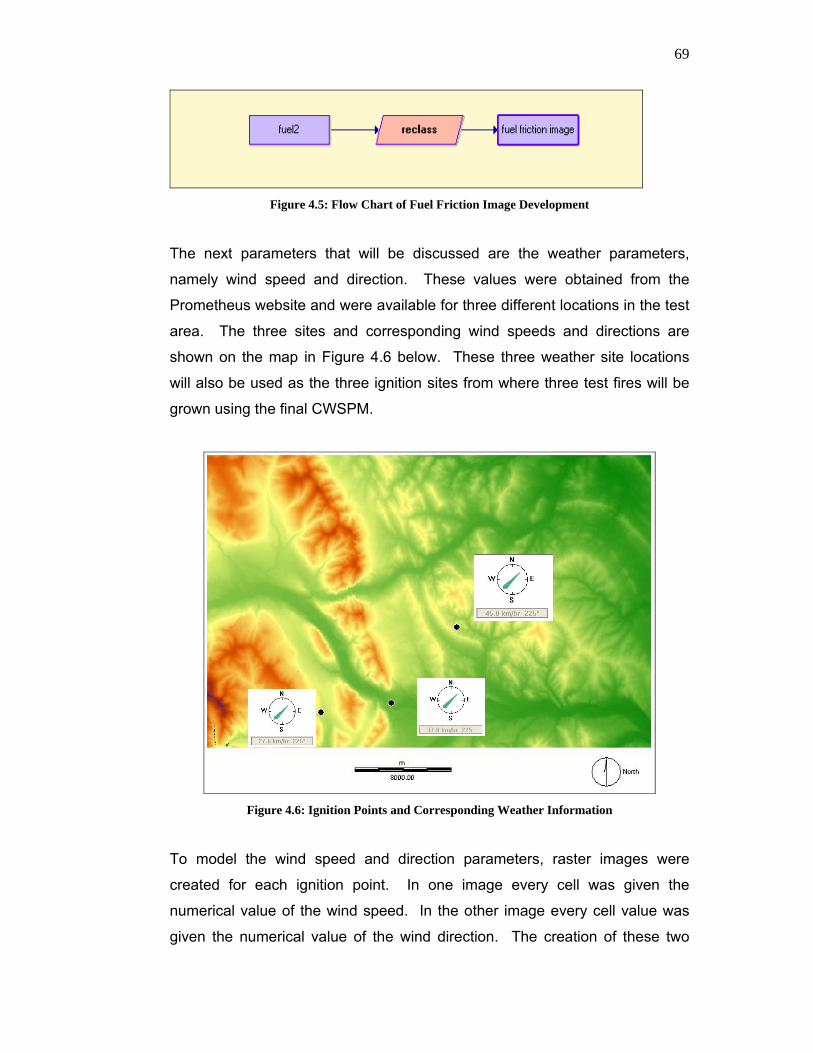
69

Figure 4.5: Flow Chart of Fuel Friction Image Development

The next parameters that will be discussed are the weather parameters,

namely wind speed and direction. These values were obtained from the

Prometheus website and were available for three different locations in the test

area. The three sites and corresponding wind speeds and directions are

shown on the map in Figure 4.6 below. These three weather site locations

will also be used as the three ignition sites from where three test fires will be

grown using the final CWSPM.

Figure 4.6: Ignition Points and Corresponding Weather Information

To model the wind speed and direction parameters, raster images were

created for each ignition point. In one image every cell was given the

numerical value of the wind speed. In the other image every cell value was

given the numerical value of the wind direction. The creation of these two

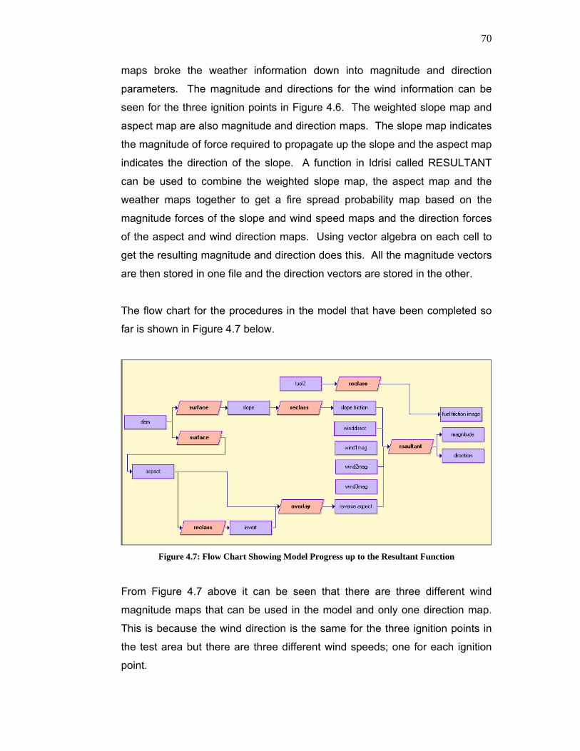
70

maps broke the weather information down into magnitude and direction

parameters. The magnitude and directions for the wind information can be

seen for the three ignition points in Figure 4.6. The weighted slope map and

aspect map are also magnitude and direction maps. The slope map indicates

the magnitude of force required to propagate up the slope and the aspect map

indicates the direction of the slope. A function in Idrisi called RESULTANT

can be used to combine the weighted slope map, the aspect map and the

weather maps together to get a fire spread probability map based on the

magnitude forces of the slope and wind speed maps and the direction forces

of the aspect and wind direction maps. Using vector algebra on each cell to

get the resulting magnitude and direction does this. All the magnitude vectors

are then stored in one file and the direction vectors are stored in the other.

The flow chart for the procedures in the model that have been completed so

far is shown in Figure 4.7 below.

Figure 4.7: Flow Chart Showing Model Progress up to the Resultant Function

From Figure 4.7 above it can be seen that there are three different wind

magnitude maps that can be used in the model and only one direction map.

This is because the wind direction is the same for the three ignition points in

the test area but there are three different wind speeds; one for each ignition

point.

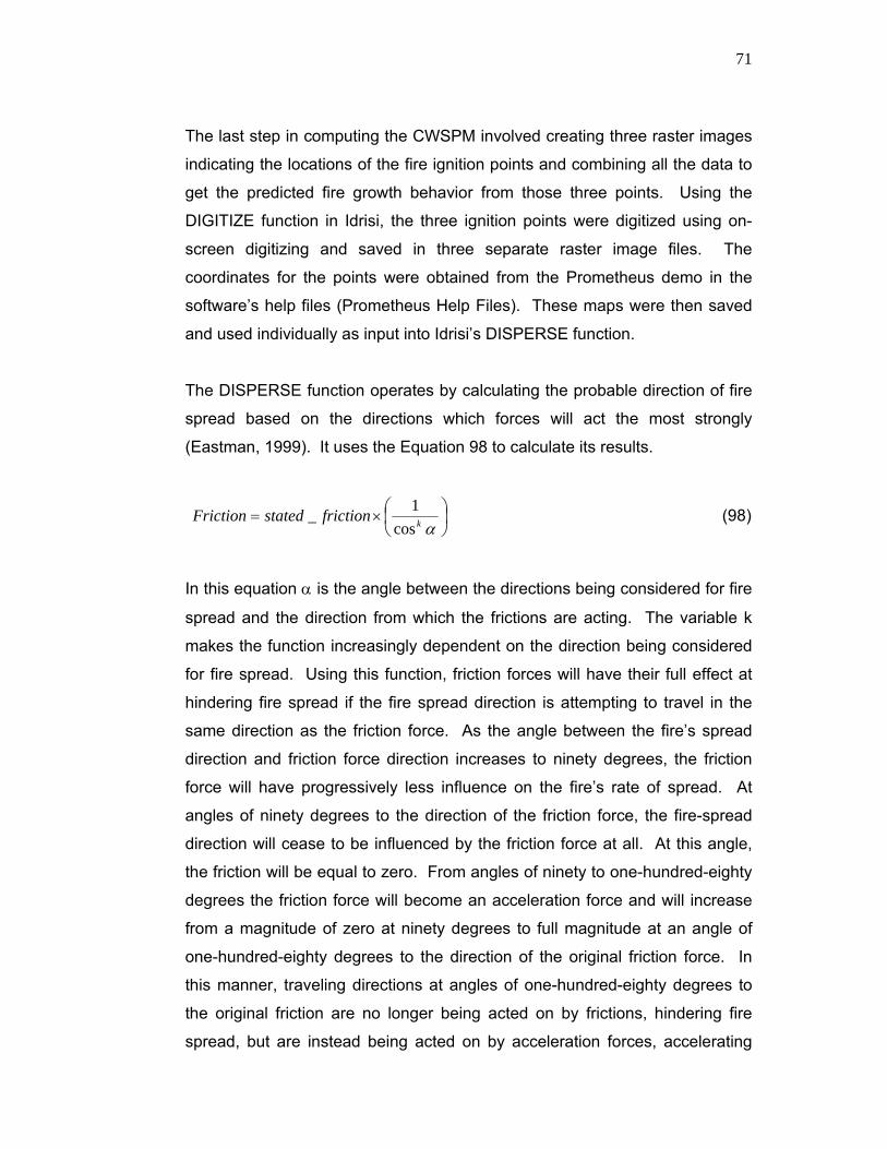
71

The last step in computing the CWSPM involved creating three raster images

indicating the locations of the fire ignition points and combining all the data to

get the predicted fire growth behavior from those three points. Using the

DIGITIZE function in Idrisi, the three ignition points were digitized using on-

screen digitizing and saved in three separate raster image files. The

coordinates for the points were obtained from the Prometheus demo in the

software’s help files (Prometheus Help Files). These maps were then saved

and used individually as input into Idrisi’s DISPERSE function.

The DISPERSE function operates by calculating the probable direction of fire

spread based on the directions which forces will act the most strongly

(Eastman, 1999). It uses the Equation 98 to calculate its results.

⎟⎠⎞

⎜⎝⎛×=

αkfrictionstatedFrictioncos

1_ (98)

In this equation α is the angle between the directions being considered for fire

spread and the direction from which the frictions are acting. The variable k

makes the function increasingly dependent on the direction being considered

for fire spread. Using this function, friction forces will have their full effect at

hindering fire spread if the fire spread direction is attempting to travel in the

same direction as the friction force. As the angle between the fire’s spread

direction and friction force direction increases to ninety degrees, the friction

force will have progressively less influence on the fire’s rate of spread. At

angles of ninety degrees to the direction of the friction force, the fire-spread

direction will cease to be influenced by the friction force at all. At this angle,

the friction will be equal to zero. From angles of ninety to one-hundred-eighty

degrees the friction force will become an acceleration force and will increase

from a magnitude of zero at ninety degrees to full magnitude at an angle of

one-hundred-eighty degrees to the direction of the original friction force. In

this manner, traveling directions at angles of one-hundred-eighty degrees to

the original friction are no longer being acted on by frictions, hindering fire

spread, but are instead being acted on by acceleration forces, accelerating

72

fire spread. A k value equal to two gives the function a nearly linear

dependency on direction. A k value equal to one-hundred makes the frictions

forces being considered degrade less rapidly as α increases to ninety

degrees. The higher the value of k, the more difficult it will be for the fire to

spread in directions other than zero degrees from the direction of the acting

force. For the purposes of the CWSPM that is being explained, the k value

was given a value of six. A value of six was chosen because direction of fire

travel plays an important roll when dealing with both slopes and wind speeds.

This chosen value was the smallest value that was capable of producing fire

probabilities where the influence of wind speed and direction could be visually

discernable. Wind speed and direction are two factors that will always have a

large influence on fire spread regardless of what direction the fire is traveling

(Principles of Fire Behavior, 1993).

To perform the DISPERSE calculation a number of raster maps are needed.

The raster maps that are used in the DISPERSE function include:

1. One of the three ignition source maps

2. The Force Magnitude map for the combined effects of slope and wind

speed

3. The Force Direction map for the combined effects of the aspect and

wind direction

4. The Fuel Friction Image map for the friction forces due to fuel type.

The flow chart indicating all the steps needed to produce a fire propagation

probability map is shown in Figure 4.8 below. The spread probability map is

shown as the last box on the far right end of the flow chart. This entire

process is run three separate times; once for each ignition point. The flow

chart below shows the set up to run the model for Ignition Point 2.

73

Figure 4.8: Final Flowchart Showing the Methodology of the CWSPM

4.3 Results of the CWSPM

Three different fire spread probability maps have been created from the

CWSPM. To help determine their accuracy three probability predictions will

be compared to an image of the actual burn perimeter, see Figure 4.9, which

was obtained from the Dogrib fire incident. This image was created on

October 21 after the fire had been extinguished.

74

Figure 4.9: Dogrib Fire Burn Perimeter (Prometheus, 2003)

The locations of the ignition points for the three CWSPM predictions are

shown in Figure 4.10 below. The area shown in both Figure 4.9 and Figure

4.10 are identical. The mountain ranges and valleys can be used to compare

the two images.

75

Figure 4.10: Locations of Ignition Points

Ignition Point 1 is located in a valley amidst a Spruce-Lichen Woodland, C-1

fuel type. The wind is traveling at an average speed of thirty kilometers per

hour and blowing from the southwest at an angle of 225 degrees. Since no

model is available to predict winds created by topography, it is anticipated that

the fire will travel in the same direction as the wind and spread towards the

river valley that lies to the north east of the ignition point. The result from the

CWSPM for the first ignition point is shown below with the DEM map set as

the background for the image.

Ignition Point 1

Ignition Point 3

Ignition Point 2

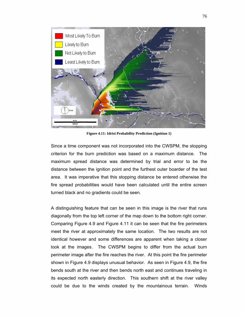
76

Figure 4.11: Idrisi Probability Prediction (Ignition 1)

Since a time component was not incorporated into the CWSPM, the stopping

criterion for the burn prediction was based on a maximum distance. The

maximum spread distance was determined by trial and error to be the

distance between the ignition point and the furthest outer boarder of the test

area. It was imperative that this stopping distance be entered otherwise the

fire spread probabilities would have been calculated until the entire screen

turned black and no gradients could be seen.

A distinguishing feature that can be seen in this image is the river that runs

diagonally from the top left corner of the map down to the bottom right corner.

Comparing Figure 4.9 and Figure 4.11 it can be seen that the fire perimeters

meet the river at approximately the same location. The two results are not

identical however and some differences are apparent when taking a closer

look at the images. The CWSPM begins to differ from the actual burn

perimeter image after the fire reaches the river. At this point the fire perimeter

shown in Figure 4.9 displays unusual behavior. As seen in Figure 4.9, the fire

bends south at the river and then bends north east and continues traveling in

its expected north easterly direction. This southern shift at the river valley

could be due to the winds created by the mountainous terrain. Winds

77

funneling through the valley could have forced the fire to travel south east until

it reached the gap in the mountains and could then burn across the foothills in

the same direction as the wind. The CWSPM also differs from the original

perimeter by displaying a definite pull in the easterly direction. The bias could

be the result of distortions appearing in the spread perimeter due to the use of

the Cellular Propagation Technique instead of the Wave Propagation

Technique. More examples involving comparisons between the two models

must be conducted before any firm conclusions can be made.

The second ignition point that will be used for comparison is located on the

north east bank of the same river reached by the fire perimeter created by

Ignition Point 1. This second fire test example uses a line ignition instead of a

point ignition to simulate a fire that has gained intensity, jumped the river and

is expanding up the far bank. Line ignitions are often used in fire behavior

predictions when an existing fire has been burning for a period of time and the

fire manager wishes to predict where the fire will travel in the future

(Prometheus, 2004). The same weights are used in this example except the

location of the fire line ignition is to the north east of the river and the wind

speed has increased from thirty kilometers per hour to forty-five kilometers per

hour. The wind direction remains constant. The relative location of this

ignition scenario can be compared to the actual burn perimeter by referring to

Figure 4.9. The fire probability prediction can be compared to the actual burn

perimeter using the river running just south of the fire as a reference.

78

Figure 4.12: Idrisi Probability Prediction (Ignition 2)

When comparing Figure 4.9 and Figure 4.12, it can be seen that both the

CWSPM and actual burn perimeter model produce similar outputs. By visual

inspection it is apparent that the two are traveling in relatively the same

direction. This example provides more consistent prediction results between

the actual burn perimeter and the CWSPM, however; the easterly bias is still

present.

The third test fire lies to the northeast of the second fire ignition scenario.

Figure 4.10 can be referenced again to determine the relative location of this

ignition in relation to the previous two. Another line ignition scenario was

utilized for this test fire spread probability prediction. For this example the

wind speed remains at forty-five kilometers per hour and the direction of the

wind continues to blow to the northeast. The results of the CWSPM can be

seen in Figure 4.13.

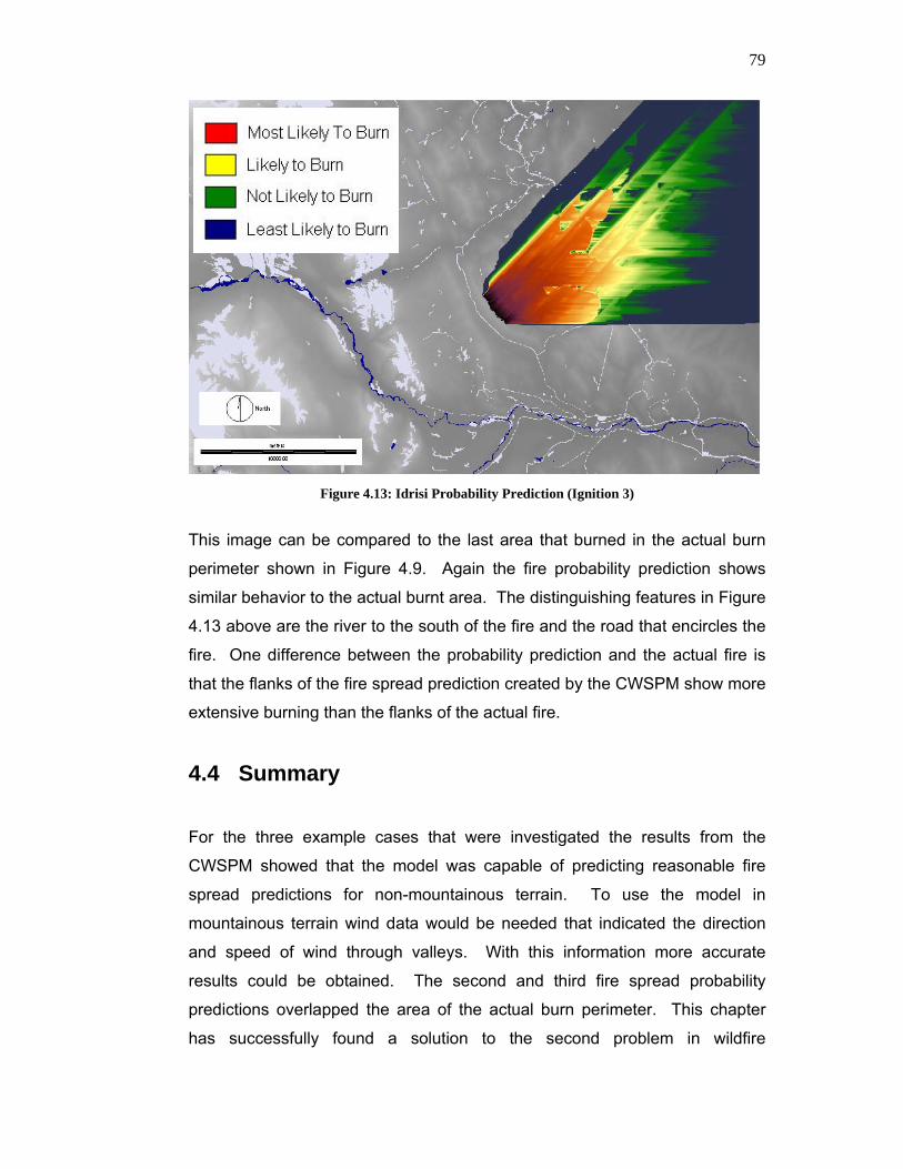
79

Figure 4.13: Idrisi Probability Prediction (Ignition 3)

This image can be compared to the last area that burned in the actual burn

perimeter shown in Figure 4.9. Again the fire probability prediction shows

similar behavior to the actual burnt area. The distinguishing features in Figure

4.13 above are the river to the south of the fire and the road that encircles the

fire. One difference between the probability prediction and the actual fire is

that the flanks of the fire spread prediction created by the CWSPM show more

extensive burning than the flanks of the actual fire.

4.4 Summary

For the three example cases that were investigated the results from the

CWSPM showed that the model was capable of predicting reasonable fire

spread predictions for non-mountainous terrain. To use the model in

mountainous terrain wind data would be needed that indicated the direction

and speed of wind through valleys. With this information more accurate

results could be obtained. The second and third fire spread probability

predictions overlapped the area of the actual burn perimeter. This chapter

has successfully found a solution to the second problem in wildfire

80

management. The development of the CWSPM fulfils the need for a

Canadian fire modeling program that improves upon the features of existing

models. The advantages of the CWSPM over the models discussed in

Chapter 3 are as follows:

• The model bases its calculations on information obtained from the

CFFDRS system. It uses Canadian standard fuel types and weights

for slope and fuel type based on calculations from the CFFDRS.

• The model can simultaneously compute a number of burn perimeter

predictions for different locations.

• Different backgrounds can be displayed behind the burn perimeter

predictions such as fuel type maps or digital elevation models.

• The model is capable of computing single burn perimeter predictions

quickly. (Less than one minute per prediction)

• The model produces successful results of predicting fire spread for

moderately flat terrain and the model’s results could be easily

improved for mountainous terrain by acquiring wind data collected in

the mountain valleys.

• The resolution of the model is dependant on the resolution of the DEM

and fuel type grids. It can therefore be altered.

Many wildfire modeling programs exist today (refer to Chapter 3) to help

managers prepare for wildfire events and create mitigation techniques to

combat wildfires. Each of these programs has varying degrees of accuracy

and, because of the limitless complexities of the environment none are one-

hundred percent accurate. Currently, Canada lacks a standard fire modeling

software program. Each fire agency in each Canadian province, and even

districts within provinces, use different programs to predict wildfire behavior

and plan suppression attacks (Trevis and El-Sheimy, 2004). The next chapter

will discuss the development of a Real-time, Internet based, wildfire

monitoring and modeling system that could be used as a prototype to develop

a Canadian standard fire modeling system.

81

It was intended for the CWSPM to be used as the fire modeling program in

this application but the development of a new standard Canadian model

dissolved this initial plan. The CWSPM can now be used as a quick, general

fire prediction model that gives the user a general idea where a fire will likely

spread to. Fire perimeter prediction models such as the new Prometheus

model can be used to more time consuming and more detailed fire

predictions. This model will be discussed in the next chapter.

82

Chapter 5: Creating an Internet Based Fire

Management System

5.1 Introduction

Wildfire management agencies have a need for a system that can estimate,

as accurately as possible, the propagation direction and intensity of spreading

wildfires. Understanding behavioral characteristics of wildfires and the way

they spread through various vegetation types and terrain is a major concern

for environmental agencies, government officials and the general public. If

unmonitored or poorly modeled, manageable fires can grow out of control and

potentially,

• Gain the intensity and heat capable of devastating entire ecosystems.

• Change local weather patterns (Principles of Fire Behavior, 1993).

• Destroy millions of dollars of prime lumber resources that are essential

to the economies of some countries (Johnson, 2001).

• Rage near cities and towns consuming the homes and assets of the

citizens (O’Brian, 2003).

Understanding wildfire behavior is critical for maintaining the safety of fire-

fighting crews and can also result in significant fiscal savings through

improved planning and resource allocation. Currently, wildfire monitoring

techniques are neither accurate nor efficient enough to optimally monitor this

natural disaster.

Accurate map information is crucial to assist ground crews, helicopters and

water bombers in mounting effective initial attacks. Airborne surveillance,

involving a spotter aircraft, a Global Positioning System (GPS) receiver and a

navigator that looks for smoke, is an invaluable tool that collects and relays

fire information to the fire managers (Rothermel, 1993). Timely

83

communication connecting the availability and deployment of bulldozers,

planes, crew and other resources is also imperative.

Currently all these facets are performed using suboptimal detection and

communication systems. Detection techniques are lacking the ability to

optimally detect hotspots that remain after the fire has been suppressed. This

creates the potential for the hotspots to re-ignite and start the fire rolling once

more. Currently in Alberta, communication is conducted using radios, which

in times of heavy fire activity become overloaded and inefficient (Wright and

El-Sheimy, 2003). It is also difficult to interpret, through verbal

communication, the exact size of the fire and the way it is expanding. Images

from spotter aircrafts are used in fire modeling but currently, these images

cannot be obtained until after the spotter aircraft has returned to the ground

base station and the fire crews have downloaded the images. To add to this

inefficiency, resource management, fire risk predictions and fire propagation

predictions are all preformed using different computer programs. Combining

an optimized fire detection system, fire resource allocation system and fire

prediction system that works in real time and links communications between

the different agencies, managers and crew would be an invaluable tool to the

future of wildfire management.

To help remedy these inefficiencies a real-time, Internet based wildfire

monitoring and modeling system has been designed to meet the fire modeling

standards of the fire agencies within Canada. This system has the potential

to impact the process of predicting wildfire propagation, resulting in reduced

damage to the environment, enhanced safety and appreciable financial

savings (Trevis and El-Sheimy, 2004). This chapter explores the design and

implementation of the Wildfire Management and Modeling System (WMMS).

It also discusses how this system could be used province-wide to help

different agencies and districts communicate more efficiently with each other

and also allow the public to view current provincial fire situations from their

personal computers.

84

As mentioned in Chapter 1 the WMMS system integrates five features into a

data acquisition/processing system and accompanying GIS based web

browser. The five features are:

1. Real time reporting of current fires,

2. Real time reporting of the spotter aircraft flight trajectories,

3. Active fires spotted by fire crews or general public

4. Fire history of each fire management district and

5. Prometheus fire behavior predictions

Combining these features, the final system is able to locate hotspots of fires

within three meters of accuracy, predict where a fire will most likely propagate

with time, detect smoldering fires under light surface vegetation, and detect

fires through smoke, haze and darkness (Wright and El-Sheimy, 2003).

Three members of the Mobile multi-sensor research group, the University of

Calgary, were actively involved in the development of this system. Bruce

Wright, a former graduate from the University of Calgary developed the Data

Acquisition System that is a component of one of the tools in the WMMS site.

For further details see (Wright, 2004). Chuanyun Fei, a former graduate from

the University of Calgary, was the site programmer. The author’s contribution

to the system involved:

• Designing the site features, general functionality, tools, and

specifications

• Designing the site’s fire modeling system (CWSPM discussed in

Chapter 4) which was later replaced with the Prometheus COM

• Testing and validating the site and Prometheus COM

• Editing and making corrections to the website interface

• Designing and programming the current form of the interface for the

entry and login screens

85

• Liaison between Alberta Sustainable Resources and the University of

Calgary. Collected and presented recommendations for the future

development of the Prometheus COM

• Determining what features Alberta Sustainable Resource Development

would like to see in an Internet based wildfire monitoring and molding

system through interviews with fire managers and fire scientists

5.2 System Architecture Design

The WMMS can be broken down into three main sub-systems. These sub-

systems can be identified as the Data Acquisition System, Control Center

System and Response System. The functionalities of each sub-system are

shown in Figure 5.1.

Figure 5.1: Three Sub-Systems of the WMMS

For the purposes of this research, an overview of the data acquisition system

will be given to inform the reader of the basics of major functionality. This

system is responsible for acquiring, controlling and storing the Wide Area

Differential Global Positioning System (WADGPS) data, Inertial Navigation

System (INS) data and the thermal camera images collected by the spotter

aircrafts during the preliminary search for new wildfires. The data collected by

this system is synchronized to a unified time frame by precisely time-tagging

all data streams using the WADGPS receiver generated Pulse per Second

(PPS) signal (Wright and El-Sheimy, 2003). These time tags can then be

used with the WADGPS and IMU data to georeference the images. The three-

Data Acquisition System • Location and time data

collection: WADGPS, INS

• Image collection: Video Camera and Thermal Camera

• Hotspot and fire line detection

Control Center System

(Web based WMMS)

• Data processing • Fire propagation

predicting • Fire status

monitoring

Response System• Information

reporting to fire managers and the general public in real-time

86

dimensional coordinates of fires and hotspots are then determined using

photogrammetric techniques after calculating the position vectors and

orientations of a pair of overlapping images.

The use of a thermal infrared camera is important for this procedure because

it senses heat emitted from objects in the form of infrared radiation and

thereby enables early detection and location of small fires that can not be

sensed by traditional cameras or the human eye. The thermal infrared

camera is also immune to factors such as haze, smoke or darkness which, in

this application, render traditional cameras useless. The process of

uploading, georeferencing and obtaining the three-dimensional coordinates of

any identified hotspots in the images occurs in real-time. At this point the

coordinate information and any corresponding images can be uploaded to an

Internet site via a telecommunications satellite.

It is anticipated that this process will allow fire managers to increase their

ability to quickly detect where hidden, smoldering fires are located. The

accuracy obtained by this system in real-time is dependant on flying height

but is generally less than five meters flying at a height of four-hundred meters

and facilitates the acquisition of accurate reports on fire position, size and

direction. For further information about this Data Acquisition System, see

Wright, 2004.

The Control Center System hosts the webpage. It has many responsibilities.

The first of three main responsibilities is archiving all information collected by

the Data Acquisition System. The second responsibility is performing the fire

behavioral modeling functions. The last major responsibility is displaying the

fire status monitoring information. More detailed information about these

processes and functions will be given in the next sections.

The last sub-system, the Response System, enables the results of the Control

Center System to be displayed to the user. This sub-system allows the

remote system user to view the results processed by the Control Center

System.

87

All three sub-systems are linked through the Web based WMMS which

organizes all functions of the Control Center System for use by the operator.

A flow chart outlining the structure of the WMMS is shown in Figure 5.2.

Figure 5.2: Flow Chart Outlining the Functions of the Control Center System

The Database Server obtains the data from the Data Acquisition System and

all data processed in the Control Center System can be viewed by the client

through the Response System. The WMMS has five main components, as

shown in Figure 5.2 that allow the three main sub-systems to communicate

seamlessly. These components are listed below:

1. Apache Web Server

2. Web MapServer

3. Hypertext Preprocessor Server (PHP)

4. Database Server

5. Transmission Control Protocol and Internet Protocol (TCP/IP)

5.2.1 Apache Web Server

The Apache Web Server is a computer platform that hosts the Web

MapServer and the PHP server. The role of the Apache Server is to connect

Get data

Apache Web Server

Web M

ap ServerUpload

data PH

P Server

Response System

Client Viewer

(HTML, JavaScript,

Java Applet)

Request Map/Image via TCP/IP

Return Map/Image via TCP/IP

Request Text via TCP/IP

Return Text via TCP/IP

Data Processing

Results

Archived Data

Get data

Upload Data

Upload Data

Query Data

Database Server

88

the client’s personal computer to the stored wildfire data on the server via the

MapServer and PHP servers.

5.2.2 Web MapServer

The Web MapServer is a public domain development environment from the

University of Minnesota that is primarily used when building spatially enabled

Internet applications. This software works on any Linux, UNIX and Windows

platform and has many GIS features that make it an attractive option for the

WMMS Webpage. MapServer also allows the clients to browse GIS data and

to create geographic maps (Lime, 2003). It is responsible for all spatial data

operations and publications created within this system (Trevis and El-Sheimy,

2004).

MapServer works by configuring each application using a text file called a

“mapfile”. Anything associated with a particular application is defined in the

mapfile as an object. In a single file there can be many objects used to build

an entire interface, or just a single object used to build a simple legend or

scale bar. To add to the functionality of the system, one can use and modify

these objects through an HTML form. The program results are then run

through a series of templates depending on the application (i.e. data browse

or feature queries) and the results are displayed to the user.

5.2.3 PHP Server

PHP is a general purpose scripting language that is particularly useful in Web

development and can be easily embedded into HTML. The PHP server

facilitates the transfer of image and textual data between the server and the

client. It performs the searching techniques of the spatial and textual data.

The user can thus access the newly published data processed by the control

center through the Apache Web Server. However, since this web based fire

modeling system is capable of publishing information in real time, the data

server must be accessed frequently. If textual, real time data is transmitted

89

the PHP server can directly transfer the data from the database to the client

via the TCP/IP protocol, which is explained later. If the data is a general

image such as fire photos, the PHP server can automatically retrieve it from

the database and pass it to the client.

5.2.4 Database Server

Multiple types of data sets are utilized in this application such as text,

spreadsheets, general and georeferenced images, GIS data and GPS

coordinates. This application uses the Standard Query Language (SQL) to

organize the database. The flexibility of the SQL language makes it easy to

separate the logical layer and data layer thus increasing its flexibility. This

database was also chosen because it can easily be transferred to a more

powerful database when extra functionality is required.

5.2.5 TCP/IP Protocol

The TCP/IP protocol is the communication protocol standard that is used in

the system to transmit data between the server computer and any number of

client computers over an Internet connection. The TCP portion of the protocol

establishes the connection between computers and exchanges streams of

data. The IP portion of the protocol addresses the packages of data and

drops them into the system so that they can be delivered to the appropriate

computer.

5.3 Interfaces for the Internet User

5.3.1 User Access and Main Page Layout

The webpage has been designed so that the first page available to the user is

a login screen that asks the users to either register or enter their user name

and password. At the time of initial registration every user is assigned a user

90

class of “general public”. This status can be upgraded to “manager” by an

existing manager who has access to the database of the system. Users with

managerial status differ from the status of general public users in the fact that

they have the ability to control, update and monitor the system. Public users

can only view, but not change, the information available in the database. To

make the webpage easily handle two classes of users, all database

manipulation tools were placed under the heading “Managers Toolbox”.

When an authorized user is logged onto the system, the program will check

the user's access rights and make available the appropriate toolbars. If a

general user is logged onto the system the Manager’s Toolbox is invisible and

cannot be accessed by the user. A sample screen capture of the WMMS is

shown in Figure 5.3. This screen capture depicts the setup for a user with

managerial capabilities. This sample can be accessed from the Internet site,

• http://cfei.geomatics.ucalgary.ca/firepub_com/firepub.php.

Figure 5.3: Screen Shot of Main Interface of the WMMS System

The left hand side of the screen shows the reference map and legend which

contain the possible layers that can be added to the display. For Figure 5.3

91

the Lakes and Rivers, Parks and Fires layers are turned on. The center of the

screen shows the province of Alberta which can be panned or zoomed-in to

any area in order to show the user a more detailed map. Currently, the

province of Alberta is shown to have four fires burning.

All fire information displayed on any map or depicted in tables and charts on

this webpage is hypothetical data and does not represent fire situations that

have happened in Alberta. This information has been temporarily entered into

the databases to test the model and webpage implementation.

On the toolbar directly above the map, fifth button from the left is a tool that

looks like a ruler. This tool is called the Nearest Distance to Lake Tool and is

able to calculate the distance between any point on the map and the nearest

major lake or river. To activate this tool one clicks on the Nearest Distance to

Lake Tool button (fifth button from the left) and then makes a second click on

any location within the main map of Alberta. This will indicate the position

from where the user wants to allocate the nearest lake. A screen shot of this

process is shown in Figure 5.4 below.

Figure 5.4: Screen Shot of Distance to Nearest Lake Tool

92

Once the user has clicked the location of interest, the nearest lake will be

highlighted in red and the distance to the lake will be displayed in decimal

degrees above the marked point. This tool could be very useful for fire

managers who are planning their initial attack on a fire and want to determine

the locations of any primary water resources.

The remaining items on the toolbar above the map of Alberta from left to right

are pan, zoom-in, zoom-out, identify, and full extents. As one uses the zoom-

in tool more detailed information regarding roads, rail and rivers appear on the

map.

Another toolbar is located on the right hand side of the screen. Each of the

tools found in this toolbar are explained individually in the next section. The

names of the tools, listed from top to bottom on the toolbar are the

Fire/Hotspot Report Tool, Trajectory Tool, Prometheus Tool and Manager’s

Toolbox.

5.4 Tools

5.4.1 Fire/Hotspot Reporting Tool

The purpose of the Fire/Hotspot Reporting Tool is to display information

pertaining to the provincial fire situation. It enables the user to view Fire

Summary Reports for the different fire districts in the province. These reports

contain information such as the number of active fires, cause of fire and fire

status. Using this tool, information can be browsed based on year or by

management district. Any fire that is currently active can be selected from

within the Fire Summary Reports and a Fire Status Page will be displayed

containing the real-time information relevant for that fire.

One of the first pieces of information displayed on the Fire Status Page is the

latitude and longitude of the center of the fire or hotspot. To help the user put

the coordinates of the fire into perspective, the location of the fire is also

93

displayed on a reference map of Alberta, shown on the same screen.

Supplementary information such as fire status, fire management district and

most up to date aerial photos are also shown on this screen. All current fire

information has the potential to be uploaded to the system in real time using

the Data Acquisition System described earlier.

5.4.2 Trajectory Tool

The second tool that is currently available on the WMMS is the Trajectory

Tool. This tool is capable of reporting the real-time trajectories of a spotter

aircraft’s flight path and displaying on the webpage the locations of any

spotted fires or hotspots along that flight path. Points along the plane’s

trajectory are collected using the WADGPS receiver that is mounted on the

spotter aircraft and transferred to the system in the same manner used by the

Fire/Hotspot Reporting Tool. The trajectories are then displayed on the base

map. Fires and hotspots are also recorded during this process and any

incoming fire coordinates are uploaded to the website and marked on the

base map with a fire icon. If the fire has been extinguished but is still

smoldering, the locations of hotspots within the smoldering area will also be

automatically uploaded to the web site as the spotter aircraft passes over.

5.4.3 Prometheus Tool

The third tool that is available on the WMMS is the Prometheus Tool. This

tool allows fire managers to determine how a current or hypothetical fire will

propagate across the terrain. Alberta Sustainable Resource Development

has permitted the Geomatics department of the University of Calgary to use

Prometheus as a tool in its WMMS system. Prometheus is currently able to

model wildfire behavior based on topography, the Canadian standard fuel

types and the Canadian standard weather index system from the Canadian

Forest Fire Danger Rating System (CFFDRS) (Prometheus, 2004).

94

Prometheus was the most recently developed fire propagation model in

Canada as of its introduction in 2003. The development of this model was

endorsed and administered by the Canadian Interagency Forest Fire Center

(CIFFC) where Alberta Sustainable Resource Development acted as the lead

agency for the project (Prometheus, 2004). Although this model has just

recently been developed, Prometheus will become the new model used by

Canadian forest fire managers. It is possible to obtain this model from the

Internet site www.firegrowthmodel.com.

Prometheus is a spatial model that uses the fire spread equations inspired by

Byram’s Fire Intensity Equation and the Wave Propagation Technique to

simulate the growth of a fire front. It is currently able to model wildfire

behavior based on topography, the algorithms of the CFFDRS discussed in

Chapter 3.

To use Prometheus the six input parameters for the FBP and FWI system

must be entered. These six parameters are:

1. Fuel type

o Determined using a list of sixteen general fuel types that are

some of the major fuel types in Canada

2. Weather

o Encapsulated using hourly data on wind speed and direction

and the output from the Fire Weather Index (FWI) System

3. Topography

o Defined by percent slope and aspect

4. Foliar moisture content

o Determined using elevation, latitude, longitude and date

5. Type and duration of prediction

o Determined using the elapsed time since the fire began and

whether it began by a point or line ignition

6. Fire line and fuel break data

95

Once these parameters are entered, the system will produce the primary

outputs of rate of fire spread, fuel consumption, head fire intensity and fire

type. From these parameters two-dimensional views can be produced to

illustrate fire spread as a function of time.

Prometheus was chosen for this system since it possesses three key

advantages that are not available together in any other model. The first

advantage is that Prometheus provides an intuitive pictorial view of the spread

of fire through the landscape. This enables users to quickly view how the fire

is spreading instead of having to interpret textual values of rate of spread and

fire intensity. The second advantage is that Prometheus uses the Fire

Behavior Prediction (FBP) and Fire Weather Index (FWI) systems of the

CFFDRS. Using the standard CFFDRS helps make Prometheus a desirable

application to use in any province or territory in Canada. Finally, Prometheus

can be integrated into the WMMS using its Microsoft COM (Component

Object Model) interface. The COM interface allows easier integration of

Prometheus with other Microsoft applications, permits additions to be made to

the model and allows the model to work seamlessly through a web browser.

The CFFDRS and Prometheus COM will be discussed in more detail in the

following sections.

5.4.3.1 Prometheus’ Component Object Model

The Prometheus COM is one feature that makes Prometheus an attractive

option for researchers. Essentially, the Prometheus COM can be described

as the Prometheus application programmed into a number of individual

components where each component makes up a piece of the original

Prometheus model. If all of the components are used together the user has

nearly all of the functionality of the original Prometheus model. The beauty of

the COM is that additions can be made to the individual components resulting

in the ability to alter the original Prometheus model so that it meets the

requirements of the researcher (Prometheus, 2003).

96

Some of the advantages of Prometheus have already been implied in the

above paragraphs however, for the sake of completeness, a list of

Prometheus’ major features is shown below (Prometheus, 2004):

• Allows users to modify fuel and weather data

• Output is compatible with Arc software

• Computes spatially explicit fire growth for single ignitions

• Uses point, line or polygon ignitions

• Uses daily or hourly weather information

• Allows user to evaluate different scenarios

• Permits the model to be altered and/or integrated with other Microsoft

applications

• Is the model that Canada will be using in the upcoming months

Despite these features Prometheus does have some limitations, such as (a) it

is incapable of using satellite images as base maps (b) it is unable to compute

fire behavior prediction perimeters for more that one ignition point at a time,

(c) it is limited to computing only eight timed perimeters for a single fire

scenario. To create larger fire perimeter predictions a larger time lapse must

be entered in between fire perimeter predictions and this can greatly affect the

performance of the model.

To use the Prometheus COM, the user must first check the structure of the

input data so that it matches the way that the COM reads input files. If the

data is not consistent a conversion must be completed so that no errors will

occur when reading the files. This conversion would be performed in the

user’s application. The converted data can then be used as input into the

Prometheus COM. The Prometheus COM Model is built using five separate

low-level COMs. Since low-level COMs are very difficult to use directly, a

higher level Prometheus COM has been built by the Alberta Sustainable

Resource Development Department to access the five separate low level

COMs (Prometheus User manual, 2004). The Prometheus COM architecture

is shown in Figure 5.5.

97

Figure 5.5: Prometheus COM Architecture

With this structure, all the functions available in the low level COMs can be

called individually and used by this system. To activate the COM on the

WMMS Webpage the user would click the “Use COM” button seen in Figure

5.4. Next, the user must go through a sequence of five screens to enter the

necessary parameters for all of the low level COMs. On the web page these

screens are designed to look like a file folder with five separate tabs. The

defining name of each screen is written on the tab of the file folder. This was

done so that the user can quickly flip back and forth between screens to enter

in all the necessary information. The first of the five screens is shown in

Figure 5.6.

User Application

Prometheus COM

Fuel COM

FWI COM

Fire Engine COM

Grid COM

Weather COM

Talk

98

Figure 5.6: Screen Shot of First Screen used to Implement COM

The information requested for each screen of the COM interface is shown in

Figure 5.7.

99

Figure 5.7: Flow Chart Describing the Necessary Parameters for the COM

Pressing the “Simulate” button on the Simulate page allows the COM to

compute a fire perimeter on the map of Alberta that is displayed on the main

page of the website. All of the variables used by the Prometheus model can

be entered in real-time to the system. This allows users to simulate fire

propagation scenarios at any time and location. After all the necessary

information is entered (projection, fuel grid, weather condition, etc.), the

website will link to the necessary components of the Prometheus COM via the

Iden

tific

atio

n Ta

b

• Used to name a simulation project (name and description).

• Name can be re-entered into the system during a subsequent user session to access the model again with the previously entered parameters intact.

Land

scap

e Ta

b

• Used for diurnal weather modeling. • Satisfies the FWI COM • Includes:

Location information to calculate the sunrise and sunset variables,

Time zone and spheroid information to convert the regional time to Greenwich Mean Time,

Elevation data to calculate the Fuel Moisture Content in the FWI module.

Mod

el

Tab

• Used to define attributes of fire behavior. • Satisfies the Fuel, Grid, FWI and Weather COMs. • Fuel grid map information describes the distribution of the

fuel types in the landscape. • Weather Station and Weather Stream specify the

parameters used in the weather model.

Scen

ario

Ta

b

• Used to define the elements influencing how fire spreads across a landscape as a function of time lapse and fire ignitions.

• Satisfies the Fire Engine COM

Sim

ulat

e

Tab

• Asks for the name of the output file that the results should be printed to.

100

PHP Server and MapServer to display an image, on the main map, of the

predicted growth perimeter for the fire.

Two example screen shots have been taken to illustrate the performance of

the Prometheus COM. These examples are of the same test site as Ignition

Point 1 that was used in the model comparison in Chapter 5. The difference

between the two images is that Figure 5.8 shows the results of the COM for

the wind speed of forty-three kilometers per hour. Figure 5.9 shows the

results for the same fire with the same parameters except the wind speed has

been changed from forty-three kilometers per hour to five kilometers per hour.

It is important to note that all topographic, fuel, elapsed burning time, and

location data is consistent between the two fires. All DEM, and fuel type

maps are identical to the parameters input into the CWSPM. To see the

parameters that were entered into the COM to obtain both image results refer

to Table 5.1. Both fires were set to burn for an eleven hour period.

Table 5.1: Parameter Entries for the Fire Perimeters of Figure 5.8 and 5.9

Wind

direction

Precipitation Max Wind

Speed

Max Temp

Figure 5.8 45 ° 0mm 43 km/h 15.8 ° C

Figure 5.9 45 ° 0mm 5 km/h 15.8 ° C

The values entered in the table were found in the help files of the Prometheus

desktop application. The results of the COM are shown below.

101

Figure 5.8: Example 1Perimeter for Fire Spread Using Prometheus COM

Figure 5.9: Example 2 of Predicted Perimeter for Fire Spread Using Prometheus COM

From Figures 5.8 and 5.9, it is evident how wind influences the predicted

spread of the fire. The decreased wind speed for Figure 5.9 has influenced

the predicted fire perimeter to take a rounder and smaller shape. In the case

of the true wind speed (Figure 5.8), the fire spreads in a direction consistent

102

with the direction of the wind and is stopped at the river bank in the same

manner as was predicted in Chapter 5.

As a further comparison Figure 5.8 can be compared to a burn perimeter

prediction calculated by the Prometheus desktop application. The perimeter

is shown in Figure 5.10 below.

Figure 5.10: Prometheus Model (Ignition 1)

Comparing the two images is apparent that there are differences between the

desktop application and the COM. The desktop application is capable of

computing multiple (up to a maximum of eight) time lapsed fire perimeters for

a single ignition. In Figure 5.10 above each perimeter is calculated at twenty

minute intervals. The consistency between the general shape of the largest

perimeter calculated by the Prometheus desktop application and the

perimeter calculated by the Prometheus COM ensures that the Prometheus

COM is operating correctly.

It must be noted that Prometheus’s COM is still under development. Version

2.0.1 is currently being used in this application. Some functions and

capabilities are currently unavailable in the COM. One such function is that

the creation of fire lines is not available. Ideally, ignitions should be specified

103

as points, lines or polygons; however the current version of the COM limits fire

ignition specifications to points only.

5.4.4 Manager’s Toolbox

Using the tools in the Manager’s Toolbox, the user can update user accounts,

update database data and update user submitted fires and hotspots.

Update User Accounts

This tool allows a manager to see information about the users who have

accessed the site. Information about the users includes:

• their user status,

• name and

• Email.

Only an existing manager can upgrade a general user to manager status.

Similarly, only a managerial user can demote a user to general status or

delete a user from the system.

Database Management Tool

This tool is still under development. Once completed, this tool will allow

users, with managerial status, to access or update the fire information

database. Data in the fire information database will include fire weather

information, provincial fuel type information and fire location information.

User Submit Fires and Hotspots Tool

This application provides tools for managing and monitoring fire and hotspot

situations. Using these tools, managers can view new fire information as it is

104

submitted by other fire managers. Managerial users can also edit or update

information about fires as it becomes available.

Wildfires and hotspots require fast response times. This system provides the

manager with the ability to work on any computer at any time, and from any

location. To ensure quick fire response times, the system will send an email

to the fire managers the instant a user submits new fire or hotspot information

to the system. In addition, having the detection software, reporting functions,

fire simulation model and decision-making support tools available on the

same website provides a seamless fire report and management tool that will

help mitigate wildfire disasters.

5.5 Summary This research has the potential to greatly benefit fire managers in predicting

and managing forest fires. This presented a solution to the third problem

existing in wildfire management. Communications between fire management

districts can be improved with the introduction of this Internet based wildfire

management and modeling system. The WMMS could help minimize

suppression efforts by directing the supplies to the areas of active heat

emissions via real-time thermal images and modeling techniques. As a result,

this system could not only save time and money but also improve the safety of

the ground based fire-fighters. This system will also be updated and

improved as future versions of the Prometheus COM are released. Additional

functions could also be created to supplement the Prometheus COM.

Proposed functions for future research are to incorporate additional variables

that affect fire behavior. Two additions could be researched. One addition

would involve the incorporation of a resource location/allocation function. The

second addition would be to include a danger vs. economic loss rating

variable into the Prometheus model.

105

Chapter 6: Conclusions and

Recommendations

6.1 Conclusions

The success of this work can be gauged by the ability to supply solutions to

the three current problems existing in wildfire management. Solutions to

these problems will greatly improve communications in the wildfire industry

and make wildfire management more efficient. The three problems are:

1. Wildfire policy does not adequately outline guidelines that should be

followed when conducting prescribed burns

2. Canadian fire modeling programs are sub optimal and should be

improved

3. Communications between fire management districts are sub optimal

and should be improved with the introduction of an Internet based

wildfire management and modeling system

Through the completion of the thesis objectives outlined in Chapter 1

solutions to the three problems have been created. The first completed

objective was to investigate the parameters that influence fire behavior and to

learn how wildfires react to various parameters in the environment. It is now

known that fires are very dependant on fuel, topography and weather.

Weather is the most influential factor in fire behavior and wind is the most

influential factor of the weather. Other parameters such as the Fine Fuel

Moisture Code and Buildup Index are also important parameters but these

parameters are used to fine tune a forest fire model and improve its precision

in wildfire modeling. Atmospheric conditions can also influence fire behavior

but these conditions are very difficult to incorporate into a model and are often

omitted. Much research is currently being conducted in this area to see how

106

atmospheric models can be merged into fire models efficiently (Clark, 1996;

Jenkins, 2002).

The second objective of this thesis was to investigate existing wildfire

management policy and to make recommendations for a prescribed fire policy

for Alberta. Since no Canadian prescribed fire policy exists, this objective was

achieved by investigating the existing American prescribed fire policies and

identifying their merits and shortcomings. Reasons for policy failure were also

investigated and recommendations were made to the future Albertan policy.

With the advent of this new policy it is hoped that runaway prescribed burns

will be reduced.

The third objective of this thesis was to investigate existing fire models and

determine their benefits and short comings to help aid the development of a

new Canadian fire model. This objective was achieved by looking at six of the

most well known fire models used in North America. Behave Plus, FireLib,

EMBYR, Farsite, FIRE! and NFDRS were analyzed. Some features from

these models that would be useful in the devlopment of a new Canadian

model are listed below:

• Spatial modeling capabilities

• Huygen’s principle of Wave Propagation for simulating the growth of a

fire front

• A methodology based on the algorithms of the CFFDRS.

• User-friendly

• Applicable for a wide range of areas

• Having the flexibility to change the resolution of the model depending

on the input data that is available

Some other features that would be useful in the development of a new

Canadian model that were not available in the researched models are listed

below:

107

• High-resolution images could be added to the background of spatial

models

• Model could be implemented on the Web so that data regarding

people and resources could be included and updated from multiple fire

stations.

• A distance to nearest water sources tool could be included in the

model

• If one zooms into the fire on the computer screen each zoom-in results

in a more detailed image on the screen

Using this information the CWSPM was developed to provide a superior

wildfire modeling tool. The results of the CWSPM are compared to an actual

burn perimeter and show good correlation with the true data. The newly

developed CWSPM is able to follow the general direction of an actual burn

perimeter. The model is able to compute fire perimeters quickly and is also

able to compute multiple fire perimeter predictions simultaneously. Such

features could be very useful to fire managers who are tying to control

multiple fires in the same area. The CWSPM is user friendly; applicable to a

wide range of areas, uses a methodology based on the CFFDRS, is flexible

enough to use a wide range of images as background maps and is capable of

being implemented on the Internet. This model was to be implemented as the

wildfire modeling system in the WMMS internet application. However, with

the development of Prometheus at the final stages of the CWSPM’s

development, it was decided not to include the CWSPM into the web

application and instead to use the Prometheus model. This was done to help

the WMMS system gain national acceptance since it uses a model that is to

become the Canadian standard modeling system.

The fourth objective of this research was to find a way to improve

communications between fire management districts with the development of

an Internet based wildfire management and modeling system. The WMMS

system is the first of its kind to combine a fire modeling system, data

acquisition system and database management system into a single program

108

capable of real time data updates. This system is also advantageous to the

general public who could use the system to view fire situations in their area or

educate themselves on fire behavior by having the freedom to grow fire

predictions on their personal computers. It is anticipated that this research

will spur fire managers to re-think the way that wildfires are managed and

promote the development of a more robust, complete fire management and

modeling system.

6.2 Recommendations

The WMMS system designed in this research is only a prototype. It will

require a number of updates to be able to function as a commercially viable

product. Tables and charts displaying historical fire data should be made to

have factual instead of hypothetical information. The graphics displaying the

fire perimeters when using the Prometheus COM could be improved. Satellite

data showing highly detailed images of highly zoomed in sites could be used

to help the user orient themselves when looking at small areas within the

Alberta map. The entire system should be tested in real-time on an actual fire

site.

It is hoped that this research will spark the imagination of some fire managers

and influence them to integrate some of the elements of the WMMS into their

own fire modeling systems (Trevis and El-Sheimy, 2004). With further

research and the continued research in fire management, hopefully wildfires

will be one natural disaster that mankind will be able to gain control of.

109

Glossary of Terms

Duff: Partially decomposed or fully decomposed layers of the forest floor.

This includes partially decomposed leaves and twigs as well as the

well-decomposed matter that rests below (Johnson, 2001).

Chutes: Steep valleys that cut into the slopes of the side of a mountain.

Chutes run parallel to the slope of a mountain and greatly influence

fire behavior by creating three up-slopes which accelerate fire spread.

Chutes also influence fire behavior by funneling the smoke column up

the chute which can increase spotting further up the mountain slope.

Crown fire: A fire involving the tree canopies or tree crowns (upper

branches) of coniferous trees.

Fine Fuels: Includes grasses, leaves, needles, and ground litter. The

moisture content of these fuels can fluctuate greatly depending on

amount of precipitation they receive (Johnson, 2001).

Fire brands: Burning embers

Fire Intensity: Based on both rate of fire spread and fuel consumption. A

fast moving fire that does not consume a lot of fuel may have the

same intensity as a slow moving fire that consumes the tree crowns

and duff layers.

Fire Spread: The rate that a fire will consume unburned vegetation and

expand its parameters.

Fuel: The vegetative substances available for burning.

Inversion: Occurs when the air temperature increases as height above the

ground increases. This is the opposite of what occurs normally.

110

Line Fire: Describes a fire that has reached a steady rate of acceleration.

Litter: The uppermost layer of ground cover on the forest floor. It is

comprised of un-decomposed leaves, twigs and branches that have

fallen from the trees and shrubs to rest on the ground (Johnson,

2001).

Point Source Fire: Describes a fire in the early stages, just after ignition.

The rate of spread of the fire is still accelerating and gaining

momentum.

Saddle Slope: Describes a depression or pass in a ridge line.

Spotting: Occurs when fire brands are lifted into the air by the updrafts

resulting from the convection currents created by a fire. These fire

brands are carried by the convection currents ahead of the current

position of the fire front. Fire brands can ignite the vegetation

surrounding the area where the firebrand was deposited and begin

new fires (Johnson, 2001).

Stable Atmosphere: Stable atmosphere is the term used to describe the

phenomenon when air temperature increases with increasing height

above the ground. Stable air restricts convection column

development and encourages more uniform and predictable burning

conditions. This condition is also known as an atmospheric inversion.

Surface Fire: A fire not involving the tree canopies or upper branches of

coniferous trees

Unstable Atmosphere: Unstable atmosphere is the term used to describe

the phenomenon when air temperature decreases with increasing

height above the ground. Unstable air allows a warm parcel of air

created by the heat of the fire to rise to great heights and establish

111

towering convection columns. The stronger the convective activity

created by the fire, the stronger the in-drafts. This increases fire

intensity and can create the conditions needed for long range

spotting.

Vortex: A whirling mass of air like a dust devil or small tornado. Vortexes

have a low pressure center which pulls in fire and objects. They can

travel in upright, vertical positions or horizontal, rolling positions

(Johnson, 2001). They are also called fire whirls.

112

References

“Alberta’s Implementation Plan for the National Forest Strategy 1998-2003,”

Progress Report for April 2000. National Forest Strategy, Alberta Sustainable

Resource Development. 2001. [cited March 12, 2004], Available:

www3.gov.ab.ca/srd/forests/fmd/nfs

Bachmann, A., and Allgöwer, B., 2000. “Error propagation in wildfire behavior

modeling”. Proceedings of the Fourth International Symposium on Spatial

Accuracy Assessment in Natural Resources and Environmental Sciences.

Delft, Delft University Press.

Bevins, C. 1996. “FireLib - User Manual and Technical Reference”.

Intermountain Research Station, Forest Service, U.S. Department of

Agriculture. Release 1.

Brown, A., Davis, K. 1973. Forest Fires Control and Use. McGraw-Hill, New

York, United States.

Cables, L., 2002. Harmonic Means. [cited Dec 31, 2004]. Available:

http://homepages.ihug.co.nz/~lcables/harmonic_means.htm

Carmody, C., 2001. Forest Fire: Context for the Canadian Forest Service’s

Science Program. Science Branch. Canadian Forest Service, Natural

Resources Canada. Ottawa.

Cerro Grande Prescribed Fire, ”Independent Review Board Report”, State of

Florida, Division of Forestry, Department of the Interior, Bureau of Land

Management. 2000.

113

Clark, T., et al. 1996. “A Coupled Atmosphere-Fire Model: Role of the

Convective Froude Number and Dynamic Fingering at the Fireline”.

International Journal of Wildland Fire. vol. 6 no. 4. Pgs. 177-190.

Clugston, Michael. 2003. “Battling the Dragon”, Canadian Geographic:

Exploration and Discovery. July/August 2003, vol. 123 no. 4. Pg. 40.

Conroy, S. Saveland, J. Beighley, M. Shive, et al. 2003. “Sanford Prescribed

Fire Review.” USDA Forest Service, March 2003. [cited March 10, 2004],

Available: www.fs.fed.us/rm/pubs

Denison, J. 1997. “Prescribed Burning for Brush Control, Brush Control for

Landowners Workshop”, USDA Natural Resources Conservation Service,

Glenwook Springs Fire Office, Newcastle, Colorado.

Doering, C. 2003. “Congress Passed Forest Thinning Bill,” World Environment

News, Planet News, November 24, 2003.

Eastman, J.R. 1999. IDRISI Guide to GIS and Image Processing. Clark

University. Vol. 2. Pgs. 130-134.

El-Sheimy, N., 2000. ENGO 431: Analytical Photogrammetry, The University

of Calgary, Calgary, Alberta.

Fernandez A., Illera P., Casanova J., 1997. “Automatic Mapping of Surfaces

Affected by Forest Fires in Spain using AVHRR NDVI Composite Image

Data”. Remote Sensing of the Environment. Vol. 60 No. 2. Pgs. 153-162.

Finney, M., 1997. “Farsite: Fire Area Simulator - User guide and technical

documentation”. Systems for Environmental Management, Version 3.0. Pgs.

156.

Finney, M., 1998. “Farsite: Fire Area Simulator – Model Development and

Evaluation”. Research Paper RMRS-RP-4, United States Department of

114

Agriculture. USDA Forest Service, Rocky Mountain Research Station. Pgs.

47.

Forestry Canada Fire Danger Group. 1992. Development and Structure of the

Canadian Forest Fire Behavior Prediction System. Forestry Canada, Ottawa,

Ontario. Information Report ST-X-3. Pgs. 62.

Forest Protection Policy Manual & Standard Operating Procedures,

Edmonton: Forest Protection, Alberta Sustainable Resource Development,

April, 2003.

Fujioka F., 2001. “A new methodology for the analysis of two-dimensional fire

spread simulations”, Fire Meteorology Research Unit. USDA Forest Services.

Riverside, CA. Pgs. 8.

Gayton, D., 1998. “Healing Fire: Sometimes Saving a Forest Means Setting it

on Fire,” Canadian Geographic: Exploration and Discovery, Vol. 118, No. 5,

July/Aug 1998.

Glickman, D., Babbit, B., et. al. 1995. Federal Wildland Fire Policy. Forest

Service Manual. USDA Forest Service.

Grabner, K., et al. 1999. "Using BEHAVE as a prescribed fire planning tool in

maintaining oak savannahs”, Notes for Forest Managers, Missouri

Department of Conservation, University of Missouri, November 1999.

Hargrove, W. et al. 2000. “Simulating fire Patterns in Heterogeneous

Landscapes,” Ecological Modeling. Elsevier, Vol. 135. Pgs. 243-263.

Healthy Forests: An Initiative for Wildfire Prevention and Stronger

Communities. Whitehouse News. 2002. [cited Feb 26th, 2004], Available:

www.whitehouse.gov/infocus/healthyforests

115

Hirsch, K. G., 1996. Canadian Forest Fire Behavior Prediction System: User’s

Guide, Vancouver, B.C., Canada, UBC Press, Pg. 1.

Hirsch, K. G., 1998. Canadian Forest Fire Behavior Prediction (FBP) System:

Interactive Training & Reference. Natural Resources Canada, Canadian

Forest Service, Northern Forestry Center. Alberta Environment Protection.

Forestry Protection Division. Edmonton, Alberta. CD-ROM.

Hunter M., 2004. “BehavePlus”. Fire Science Lab and Systems for

Environmental Management. [cited: December 8, 2004] Available:

www.fire.org.

“Jack Pine Ecosystem,” Department of Natural Resources, Michigan

Government Website, Updated: Jan 29, 2003, [cited March 10, 2004],

Available: www.michigan.gov. 2003.

Jenkins, M., 2002. “An Examination of the Sensitivity of Numerically

Simulated Wildfires to Low-level Atmospheric Stability and Moisture, and the

Consequences for the Haines Index”. International Journal of Wildland Fire,

vol. 11. Pgs 1-20.

Johnson, E. A., Miyanishi, K., 2001. Forest Fires: Behavior and Ecological

Effects, San Diego, CA, U.S.A., Academic Press. Pgs. 529-532.

Knapp, L., Andrews, P., Turek, J., 1996. “Image Navigation for Wildland Fire

Location Mapping”. NCGIA Conference on GIS and Environmental Modeling.

January 21-24, 1996. Santa Fe, New Mexico.

Kehr M. 2004. RPFT, Prescribed Fire Operational Coordinator, Wildfire

Operations Section, Alberta Sustainable Resources, email sent March 2nd

2004.

116

Koehler, J., 1997. “The Use of Prescribed Burning as a Wildfire Prevention

Tool", Florida Forestry Division, [cited Feb 26, 2004], Available: http://flame.fl-

dof.com/Env/koehler.html

Lime, S., 2003. Information about Map Server, “Map Server: Current Version

4.0.2”, University of Minnesota, USA. [cited: June 16, 2003] Available:

http://mapserver.gis.umn.edu.

“Lowden Ranch Prescribed Fire Review”, U.S. Department of the Interior,

Bureau of Land Management. 1999.

Mahmud, M., 1999. “Forest Fire Monitoring and Mapping in South East Asia”.

National Seminar on LUCC and GOFC (NASA/EOC). Nov 12 1999. Bangi.

Pgs. 8.

Monmonier, M., 1982. Computer Assisted Cartography: Principles and

Prospects. Englewood cliffs, N.J., Prentice-Hall Inc. Pgs. 76-79.

O’Brian, 2003. “A Confusion hurt effort: Kelowna fire chief: Plea made to

make decisions locally”. Thursday, November 27, 2003. Vancouver Sun.

Parsons, D. 1978. “Fire and Fuel Accumulation in a Giant Sequoia Forest”,

Journal of Forestry, Vol. 76, No. 2, February, 1978.

Principles of Fire Behavior. 1993. Compact Disk. Environmental Training

Center. Hilton, Alberta, Canada. ISBN:0-7785-0073-X

Prometheus COM Programmer’s Manual, CWFGM Project Steering

Committee, Alberta Sustainable Resources Department, July 2003.

Prometheus User Manual. Alberta Sustainable Development. Version 3.0.1,

2004.

117

Rothermel, R. C. 1972. “A mathematical model for predicting fire spread in

wildland fuels”. Research Paper INT-115. Ogden, UT: U.S. Department of

Agriculture, Forest Service, Intermountain Forest and Range Experiment

Station. Pgs. 40.

Rothermel, R.C., 1993. “Mann gulch fire: a race that couldn’t be won”, United

States Department of Agriculture, Forest Service, General Technical Report,

INT-299, Intermountain Research Station, Ogden, Utah. Pgs. 10.

Sannier C., Taylor J., 2002. “Real-time Monitoring of Vegetation Biomass with

NOAA-AAVHRR in Etosha National Park, Namibia, for Fire Risk Assessment”.

International Journal of Remote Sensing 23(1): Pgs. 71-89.

“Sawtooth Mountain Prescribed Fire Burnover Fatality: Factual Report”,

Bureau of Indian Affairs, Fort Apache Agency, Arizona. 2003.

Super, S.M., 2002. “Zero Code, WO Amendment 5100-2000-2. Forest Service

Manual Directive Issuances, 6700 – Safety and Health Program”. Rocky

Mountain Research Station. USDA Forest Service. Washington, DC.

The State of Canada’s Forests – Forests in the New Millennium, The National

Library of Canada. Natural Resources Canada. Ottawa, Ontario. 2000.

Trevis, L., El-Sheimy, N., 2004. “The Development of a Real-Time Fire

Monitoring and Management System”. The XXth International Symposium for

Photogrammetry and Remote Sensing. Istanbul, Turkey, July 2004.

Tymstra, C. et al. 1999. “Proposal to the Foothills Model Forest Development

and Application of a Wildland Fire Growth Model”. Alberta Sustainable

Resources Department. April 1999.

Understanding the Fire Weather Index System. Compact Disk. The

Environmental Training Center. Hilton, Alberta, Canada. ISBN: 0-7785-0076-4

118

“Urban-Wild land Interface Fire: The I-Zone Series. Chapter VIII: Fire

Behavior Modeling”. University of California, Forest Products Laboratory.

[Available]: http://www.ucfpl.ucop.edu/I-Zone/IZoneIndex.htm

Van Wagner, C.E.; Pickett, T.L. 1985. Equations and FORTRAN program for

the Canadian Forest Fire Weather Index System. Canadian Forest Service,

Ottawa, Ontario. Forestry Technical Report 33.

Van Wagner, C.E. 1987. Development and structure of the Canadian Forest

Fire Weather Index System. Canadian Forestry Service. Ottawa, Ontario.

Forestry Technical Report 35. Pgs. 36.

Weinstein, D., et al. 1995. “Fire Growth Modeling in and Integrated GIS

Environment”. ESRI International Users Conference. Palm Springs, California.

May 22-26, 1995

“Wildfire Detection”. Sustainable Resource Development. [cited: Jan 12, 2005]

[Available]: www3.gov.ab.ca/srd/wildfires/fpd/fw_wd.cfm. 2004.

Wright, D.B.,"A Feasibility Study for Real-Time Detection and Georeferencing

of Forest Fire Hot Spots", M.Sc. Thesis, Department of Geomatics

Engineering, University of Calgary, June, 2004.

Wright, B. and El-Sheimy, N., 2003: "Real-Time Direct Georeferencing of

Thermal Images for Identification and Location of Forest Fire Hotspots”, 6th

Conference on Optical 3D Measurement Techniques, Zurich, Switzerland,

September 22-25, 2003.

Wearth, John, 2004. “National Fire Danger Rating System”, National Fire

Danger Rating System. Available:

http://www.seawfo.noaa.gov/fire/olm/nfdrs.htm

Zimmerman, G., Bunnel, D., 1998. “Wildland Prescribed Fire Management

Policy”. Implementation Procedures Reference Guide, USDA Forest Service.

119

Resources

Bhardwaj, M. 2003, “Let it Burn! Why Canada’s National Parks Use Fire to

Prevent Fire,” Canadian Geographic: Exploration and Discovery et cetera,

July/Aug 2003.

Ealey, D., 2004. “Forest Sustainability,” Alberta Sustainable Resource

Development, [cited Feb 26, 2004], Available:

www3.gov.ab.ca/srd/forests/managing/sustain

“Sustainable Development Course Overview,” class notes for EVDS 683.50,

Department of Environmental Design, University of Calgary, Winter 2002.

120

Appendices

Appendix A: Surface Fuel Consumption Curves

Figure A1: Surface Fuel Consumption Curves for Fuel Types C1-C7, M3, M4 and D1

(Van Wagner, 1987)

121

Figure A2: FFC and WFC Curves for S Fuel Types (Van Wagner, 1987)

122

Appendix B: Rate of Spread Curves

Figure B2: ROS Curves for C1 - C6 Fuel Types (Van Wagner, 1987)

123

Figure B3: ROS Curves for C7, D1, and S Fuel Types (Van Wagner, 1987)

124

Figure B4: ROS Curves for M Class Fuel Types (Van Wagner, 1987)

Figure B5: ROS Plot for Matted Grass Figure B6: ROS Plot for Standing Grass (Van Wagner, 1987) (Van Wagner, 1987)

125

125

Appendix C: Methodology for CWSPM Fuel Type Weights

Table C1: Parameters Entered into Eleven ROS Scenarios Run 1 Run 2 Run 3 Run 4 Run 5 Run 6 Run 8 Run 9 Run 10 Run 11Month 6 6 6 6 6 6 6 6 6 6 Day 1 1 1 1 1 1 1 1 1 1 BUI 40 70 70 70 40 40 50 100 90 50 FFMC 90 90 99 85 99 85 85 95 95 70 Latitude 55 55 55 55 55 55 55 55 55 55 Longitude 110 110 110 110 110 110 110 110 110 110 Elevation 0 0 0 0 0 0 0 0 0 0 Ignition Point Point Point Point Point Point Point Point Point Point Wind speed 0 0 0 0 0 0 0 0 0 0 % Slope 0 0 0 0 0 0 0 0 0 0 Elapsed Time 30 30 30 30 30 30 30 30 30 30

126

Table C 2: ROS for all Fuel Types for the Eleven Scenarios Run 1 Run 2 Run 3 Run 4 Run 5 Run 6 Run 7 Run 8 Run 9 Run 10 Run 11C1 0.1 0.2 10.2 0 9.6 0 0 2.1 2 0 0 C2 3.6 4.3 22.4 1.6 18.5 1.3 1.4 12.3 12 0.2 0.6 C3 0.5 0.6 12.6 0.1 10.8 0.1 0.1 3.9 3.8 0 0 C4 4 4.5 23.1 1.6 20.5 1.4 1.5 12.4 12.2 0.3 0.7 C5 0.1 0.1 5.3 0 4.7 0 0 1.4 1.4 0 0 C6 0.7 0.7 29.2 0.1 9.1 0.1 0.1 7.4 5.3 0 0 C7 0.6 0.6 5.7 0.2 5.2 0.2 0.2 2.4 2.4 0 0.1 M1-25 1.5 1.7 9.1 0.6 8.1 0.5 0.6 4.7 4.7 0.1 0.2 M1-75 3.2 3.6 18.6 1.3 16.5 1.1 1.2 9.8 9.7 0.2 0.5 M2-25 1.1 1.2 6.5 0.4 5.8 0.4 0.4 3.4 3.4 0.1 0.2 M2-75 3 3.4 17.7 1.2 15.7 1.1 1.2 9.4 9.3 0.2 0.5 M3-25 0.7 0.7 4.7 0.2 4.2 0.2 0.2 2.3 2.2 0 0.1 M3-75 9.1 10.3 44.4 3.9 39.4 3.5 3.7 26 25.7 0.7 1.6 M4-25 0.3 0.3 5.2 0.1 4.6 0.1 0.1 1.9 1.9 0 0 M4-75 3.3 3.7 23.2 1.1 20.6 1 1.1 11.6 11.4 0.1 0.4 D1 0.7 0.8 4.5 0.3 4.3 0.2 0.2 2.2 2.2 0 0.1 S1 4.8 5.6 23.2 2.3 19.9 2 2.1 13.8 13.6 0.5 1.1 S2 1.7 2 11.6 0.7 9.9 0.6 0.6 6.1 6 0.1 0.2 S3 1.3 1.5 23.4 0.2 20.1 0.2 0.2 8.9 8.8 0 0 O1a 6.2 6.2 28.1 2.4 28.1 2.4 2.4 15 15 0.5 1 O1b 5.3 5.3 32.1 1.7 32.1 1.7 1.7 15.3 15.3 0.2 0.6

1