Universal digital quantum simulation with trapped ions

B. P. Lanyon1,2∗, C. Hempel1,2, D. Nigg2, M. Muller1,3, R. Gerritsma1,2,F. Zahringer1,2, P. Schindler2, J. T. Barreiro2, M. Rambach1,2, G. Kirchmair1,2,

M. Hennrich2, P. Zoller1,3, R. Blatt1,2, C. F. Roos1,2.

1Institut fur Quantenoptik und QuanteninformationOsterreichische Akademie der Wissenschaften,

Otto-Hittmair-Platz 1, A-6020 Innsbruck, Austria,2Institut fur Experimentalphysik, University of Innsbruck,

Technikerstr. 25, A-6020 Innsbruck, Austria,3Institut fur Theoretische Physik, University of Innsbruck,

Technikerstr. 25, A-6020 Innsbruck, Austria.∗To whom correspondence should be addressed; E-mail: ben.lanyon@uibk.ac.at

A digital quantum simulator is an envisioned quantum device that can be pro-

grammed to efficiently simulate any other local system. We demonstrate and

investigate the digital approach to quantum simulation in a system of trapped

ions. Using sequences of up to 100 gates and 6 qubits, the full time dynamics

of a range of spin systems are digitally simulated. Interactions beyond those

naturally present in our simulator are accurately reproduced and quantitative

bounds are provided for the overall simulation quality. Our results demon-

strate the key principles of digital quantum simulation and provide evidence

that the level of control required for a full-scale device is within reach.

While many natural phenomena are accurately described by the laws of quantum mechan-

ics, solving the associated equations to calculate properties of physical systems, i.e. simulating

1

arX

iv:1

109.

1512

v2 [

quan

t-ph

] 7

Oct

201

1

quantum physics, is in general thought to be very difficult (1). Both the number of parameters

and differential equations that describe a quantum state and its dynamics, grow exponentially

with the number of particles involved. One proposed solution is to build a highly controllable

quantum system that can efficiently perform the simulations (2). Recently, quantum simula-

tions have been performed in several different systems (3–12), largely following the analog

approach (2) whereby an analogous model is built, with a direct mapping between the state and

dynamics of the simulated system and those of the simulator. An analog simulator is dedicated

to a particular problem, or class of problems.

A digital quantum simulator (2, 13–15) is a precisely controllable many-body quantum sys-

tem on which a universal set of quantum operations (gates) can be performed, i.e. a quantum

computer (16). The simulated state is encoded in a register of quantum information carriers,

and the dynamics are approximated with a stroboscopic sequence of quantum gates. What

makes this device so special is that it can, in principle, be reprogrammed to efficiently simulate

any local quantum system (13) and is therefore referred to as a universal quantum simulator.

Furthermore, there are known methods to efficiently correct for and quantitatively bound exper-

imental error in large-scale digital simulations (17).

We report on digital simulations using a system of trapped ions. We focus on simulat-

ing the full time evolution of networks of interacting spin-1/2 particles, which are models of

magnetism (18) and exhibit rich dynamics. We do not use error correction, which has been

demonstrated separately in our system (19), and must be included in a full-scale fault-tolerant

digital quantum simulator.

The central goal of a quantum simulation is to calculate the time-evolved state of a quan-

tum system ψ(t). In the case of a time-independent Hamiltonian H the form of the solution is

ψ(t)=e−iHt/~ψ(0)=Uψ(0). A digital quantum simulator can solve this equation efficiently for any

local quantum system (13), i.e. where H contains a sum of terms Hk that operate on a finite

2

number of particles, due to interaction strengths that fall of with distance for example. In this

case the local evolution operators Uk = e−iHkt/~ can be approximated using a fixed number of op-

erations from a universal set. However, these terms do not generally commute U ,∏

k e−iHkt/~.

This can be overcome using the Trotter approximation (13, 20), e−iHt = limn→∞(∏

k e−i~Hkt/n)n,

for integer n, which is at the heart of the digital quantum simulation algorithm. For finite n the

Trotter error is bounded and can be made arbitrarily small. The global evolution of a quantum

system can therefore be approximated by a stroboscopic sequence of many small time-steps of

evolution due to the local interactions present in the system. The digital algorithm can also be

applied to time-dependent Hamiltonians and open quantum systems (13, 15, 16, 21).

Our simulator is based on a string of electrically trapped and laser-cooled calcium ions

(see (22)). The |S 1/2〉=|1〉 and |D5/2〉=|0〉 Zeeman states encode a qubit in each ion. Simulated

states are encoded in these qubits and manipulated by laser pulses that implement the operation

set: O1(θ, j) = exp(−iθσ jz); O2(θ) = exp(−iθ

∑i σ

iz); O3(θ, φ) = exp(−iθ

∑i σ

iφ); O4(θ, φ) =

exp(−iθ∑

i< j σiφσ

jφ). Here σφ= cos φσx + sin φσy and σ j

k denotes the k-th Pauli matrix acting

on the j-th qubit. O4 is an effective qubit-qubit interaction mediated by a common vibrational

mode of the ion string (23). Recent advances have seen the quality of these operations increase

appreciably (24). For our simulations, we define dimensionless Hamiltonians H, i.e. H=EH

such that U=e−iHEt/~ and the system evolution is quantified by a unitless phase θ=Et/~.

We begin by simulating an Ising system of two interacting spin-1/2 particles, which is an

elementary building block of larger and more complex spin models, and was one of the first sys-

tems to be simulated with trapped ions following an analog approach (6, 25). The Hamiltonian

is given by HIsing=B(σ1z + σ2

z ) + Jσ1xσ

2x. The first bracketed term represents the interaction of

each spin with a uniform magnetic field in the z-direction and the second an interaction between

the spins in an orthogonal direction. The interactions do not commute, giving rise to non-trivial

dynamics and entangled eigenstates. Each spin is mapped directly to an ionic qubit (|1〉=| ↑〉,

3

|0〉=| ↓〉). The dynamics are implemented with a stroboscopic sequence of O2 and O4 gates, rep-

resenting the magnetic field and spin-spin evolution operators, respectively. We first simulate

a time-independent case J=2B which couples the initial state | ↑↑〉 to a maximally entangled

superposition of |↑↑〉 and |↓↓〉 (Fig 1A). The simulated dynamics converge closer to the exact

dynamics as the digital resolution is increased. The overall simulation quality is quantified us-

ing quantum process tomography (QPT) (26), yielding a process fidelity of 91(1)% at the finest

digital resolution used. In (22) we show how higher-order Trotter decompositions can be used

to achieve more accurate digital approximations with fewer operations.

We now consider a time-dependent case where J increases linearly from 0 to 4B during

a total evolution θt. In the limit θt→∞, spins initially prepared in the paramagnetic ground

state of the magnetic field (|↓↓〉) will evolve adiabatically into the anti-ferromagnetic ground

state of the final Hamiltonian: an entangled superposition of the∑

j σjx eigenstates |←→〉x and

|→←〉x. As a demonstration, we approximate the continuous dynamics, for θt=π/2, using a

stroboscopic sequence of 24 O2 and O4 gates, and measure the populations in the σx basis

(Fig 1B). The evolution closely follows the exact case and an entangled state is created (63(6)%

tangle (27)). Full quantum state reconstructions are performed after each digital step, yielding

fidelities between the ideal digitised and measured state of at least 91(2)%, and overlaps with

the instantaneous ground state of no less than 91(2)%. Note that the observed oscillation in

expectation values is a diabatic effect, as excited states become populated.

More complex systems with additional spin-spin interactions in the y (‘XY’ model) and z

(‘XYZ’ model) directions can be simulated by reprogramming the operation sequence. The

dynamics due to an additional spin-spin interaction in the y-direction is simulated by adding

another O4 operation to each step of the Ising stroboscopic sequence (with φ=π/2). A third

spin-spin interaction in the z-direction is realised by adding an O4 gate sandwiched between a

pair of O3 operations set to rotate the reference frame of the qubits. In the simulated dynamics

4

of the initial state |→←〉x under each model, for a fixed digital resolution of θ/n=π/16 and

up to 12 trotter steps (Fig 2), up to 24, 48 and 84 gates are used for the Ising, XY and XYZ

simulations, respectively. This particular initial state is chosen because the ideal evolution is

different for each model. The results show close agreement with the exact dynamics and results

from QPT after four digital steps yield process fidelities, with the exact unitary evolution, of

88(1)%, 85(1)% and 79(1)%, for the Ising, XY and XYZ respectively. With perfect operations

the Trotter error would be less than 1% in each case. Note that while analog simulations of

Ising models have previously been demonstrated in ion traps (6, 8), XY and XYZ models have

not.

The digital approach allows arbitrary interaction distributions between spins to be pro-

grammed. For three-spin systems, we realise various interactions that give rise to the dynamical

evolutions of the initial state | ↑↑↑〉 (Fig 3). Fig 3A shows a system supporting interactions

between all spin pairs with equal strength, and between each spin and a transverse field. The

initial state couples equally to | ↑↓↓〉, | ↓↑↓〉 and | ↓↓↑〉, while the strength of the field determines

the amplitude and frequency of the dynamics. For the case shown (J = 2B) an equal superpo-

sition of the coupled states is periodically created (an entangled W state (28)). Fig 3B shows

how non-symmetric interaction distributions can be programmed, using sequences of O4 and

O1 to add spin-selective interactions. The interaction between one spin pair is dominant. Due

to this broken symmetry, one coupled state (| ↑↓↓〉) is populated faster than the others, yielding

more complex dynamics than in the symmetric case. Fig 3C demonstrates the ability to sim-

ulate n-body interactions; specifically σ1zσ

2xσ

3x. A clear signature is observed: direct coupling

between∑

j σjy eigenstates |→→→〉y and |←←←〉y, periodically producing an entangled GHZ

state (28). Many-body spin interaction of this kind are an important ingredient in the simula-

tion of systems with strict symmetry requirements (29) or spin models exhibiting topological

order (30)”. Measurements in other bases and simulations of nearest-neighbour and many-body

5

interactions with a transverse field using over 100 gates are presented in (22).

Fig 4A shows the observed dynamics of the 4-spin state | ↑↑↑↑〉 under a long-range Ising-

type interaction. The rich structure of the dynamics reflects the increased complexity of the

underlying Hamiltonian: oscillation frequencies correspond to the energy gaps in the spec-

trum. This information can be extracted via a Fourier transform of the data (see (22)). Specific

energy gaps could be targeted by preparing superpositions of eigenstates via an initial quasi-

adiabatic digital evolution (10), or study the complex non-local correlations generated by this

model. Fig 4B shows the observed dynamics for our largest simulation: a six spin many-body

interaction, which directly couples the states | ↑↑↑↑↑↑〉 and | ↓↓↓↓↓↓〉, periodically producing a

maximally entangled GHZ state.

Direct quantification of simulation quality for more than two qubits is impractical via QPT:

for three qubits, expectation values must be measured for 1728 experimental configurations, and

this increases exponentially with qubit number (≈ 3× 106 for six qubits). However, the average

process fidelity (Fp) can be bounded more efficiently (31). We demonstrate this for the 3- and

6-spin simulations of Fig 3C and 4B, respectively. Bounds of 85(1)%≤Fp≤91(1)% (3 spins)

and 56(1)%≤Fp≤77(1)% (six spins) are obtained at φ=0.25, using 40 and 512 experimental

configurations respectively (22). The largest system for which a process fidelity has previously

been measured is 3 qubits (32). Note that a different measure of process quality is given by the

worst-case fidelity, over all input states, and may be better used to assess errors in future full-

scale fault-tolerant simulations. Regardless of the measure used, the error in large-scale digital

simulations built from finite-sized operations can be efficiently estimated. Each operation can

be characterized with a finite number of measurements, then the error in any combination can

be chained (33). In order to exploit this the number of ionic qubits on which our many-qubit

operators O2−4 can act must be restricted.

The dominant effect of experimental error can be seen in Fig 3B and 4B: the dynamics

6

damps due to decoherence processes. Laser frequency and ambient magnetic field fluctuations

are far from the leading error source: in the absence of coherent operations, qubit lifetimes are

over an order of magnitude longer (coherence times ≈ 30 ms) than the duration of experiments

(≈ 1−2 ms). The current leading sources of error, which limit both the simulation complexity

and size, are thought to be laser intensity fluctuations (22). This is not currently a fundamental

limitation and, once properly addressed, should enable an increase in simulation capabilities.

The digital approach can be combined with existing tools and techniques for analog simu-

lations to expand the range of systems that can be simulated. In light of the present work, and

current ion trap development (34), digital quantum simulations involving many tens of qubits

and hundreds of high-fidelity gates seems feasible in coming years.

Acknowledgements

We thank Wolfgang Dur, Alan Aspuru-Guzik and Michael Brownnutt for discussions. We ac-

knowledge financial support by the Austrian Science Fund (FOQUS), the European Commis-

sion (AQUTE), the Institut fur Quanteninformation GmbH, IARPA, and two Marie Curie Inter-

national Incoming Fellowships within the 7th European Community Framework Programme.

7

Fig. 1. Digital simulations of a two-spin Ising system. Dynamics of initial state | ↓↓〉 fortwo cases. (A) a time independent system (J=2B) and increasing levels of digital resolution(i→iv.). A single digital step is D.C=O4(θa/n, 0).O2(θa/2n), where θa=π/2

√2 and n=1, 2, 3, 4

(for panels i.-iv respectively). Quantum process fidelities between the measured and exact sim-ulation at θa are i) 61(1)% and iv) 91(1)% (ideally 61% and 98%, respectively) (1). (B) A time-dependent system. J increases linearly from 0 to 4B. Percentages: fidelities between measuredand exact states with uncertainties less than 2%. The initial and final state have entanglement0(1)% and 63(6)% (tangle (27)), respectively. The digitised linear ramp is shown at the bottom:c=O2(π/16), d=O4(π/16, 0). For more details see (22). Lines; exact dynamics. Unfilled shapes;ideal digitised. Filled shapes; data (↑↑ _↓↓ →→x N←←x).

8

Fig. 2. Digital simulations of increasingly complex two-spin systems. Dynamics of the initialstate | →←〉x using a fixed digital resolution of π/16. The graphic in each panel shows how asingle digital step is built: C=O2(π/16), D=O4(π/16, 0), E=O4(π/16, π), F=O3(π/4, 0). Quan-tum process fidelities between the measured and exact simulation after 1 and 4 digital steps areshown with grey arrows (uncertainties ≤ 1% (22)). Lines; exact dynamics. Unfilled shapes;ideal digitised. Filled shapes; data (_→←x ←→x N←←x,→→x).

9

Fig. 3. Digital simulations of three-spin systems. Dynamics of the initial state | ↑↑↑〉 inthree cases. (A) Long-range Ising system. Spin-spin coupling between all pairs with equalstrength and a transverse field. C=O2(π/32), D=O4(π/16, 0). (B) Inhomogeneous distributionof spin-spin couplings, decomposed into an equal strength interaction and another with twicethe strength between one pair. E=O1(π/2, 1). (C) Three-body interaction, which couples the∑

j σjy eigenstates | ←←←〉y and | →→→〉y. An O3(π/4, 0) operation before measurement ro-

tates the state into the logical σz basis. F=O1(θ, 1), 4D=O4(π/4, 0). Any point in the phaseevolution is simulated by varying the phase θ of operation F. Inequalities bound the quantumprocess fidelity Fp (see (22) for details).

10

Fig. 4. Digital simulations of four and six spin systems. Dynamics of the initial state whereall spins point up in two cases. (A) Four spin long-range Ising system. Each digital step isD.C=O4(π/16, 0).O2(π/32). Error bars are smaller than point size. (B) Six spin six-body in-teraction. F=O1(θ, 1), 4D=O4(π/4, 0). The inequality at φ=0.25 bounds the quantum processfidelity Fp at θ=0.25 (see (22) for details). Lines; exact dynamics. Unfilled shapes; ideal digi-tised. Filled shapes; data (P0 _P1 P2 NP3 IP4 HP5 JP6, where Pi is the total probability offinding i spins pointing down.)

11

Supplementary Online Material

1 Experimental details

For each simulation a string of 40Ca+ ions is loaded into a linear Paul trap. Qubits are encoded

in two internal states of each ion. We use the meta-stable (lifetime ∼ 1 s) | ↑〉 = |D5/2,m j = 3/2〉

state and the | ↓〉 = |S 1/2,m j = 1/2〉 ground state, where m j is the magnetic quantum number,

for the experiments with 2 ions and | ↑〉 = |D5/2,m j = −1/2〉, | ↓〉 = |S 1/2,m j = −1/2〉 for the

experiments with more ions. These states are connected via an electric quadrupole transition

at 729 nm and an ultra-stable laser is used to perform qubit operations. At the start of each

experiment the ions are Doppler cooled on the S 1/2 ↔ P1/2 transition at 397 nm. Optical

pumping and resolved-sideband cooling on the | ↓〉 ↔ |D5/2,m j = 5/2〉 transition prepare the

ions in the state | ↓〉 and in the ground state of the axial center-of-mass vibrational mode.

The internal states of the ions are measured by collecting fluorescence light on the S 1/2 ↔

P1/2 transition on a photomultiplier tube and/or CCD camera. Instances where fluorescence light

is detected correspond to the ion being in the state | ↓〉, instances where it is not correspond to

the ion being in state | ↑〉. Each simulation experiment (consisting of cooling, state preparation,

simulated time evolution and detection) is repeated many times to obtain enough statistics (at

least 200 times per data point). The photomultiplier measures the collective fluorescence state

of the ion string, from which the probability for any number of ions in the string to be bright

can be extracted i.e. P0 (probability for 0 ions being bright), P1 (probability for any 1 ion to be

bright) etc. More information can be obtained by using the CCD camera. By defining regions

of interest on the camera sensor, the fluorescence of each ion can be measured individually,

from which the logical state of any individual ion can be extracted. Measurements in other

bases are achieved by applying single-qubit operations to the ions before measurement, to map

eigenstates of the desired observable to the logical eigenstates.

12

More detailed information about our experimental setup and techniques can be found in the

Ph.D. thesis of Gerhard Kirchmair (35).

Quantum simulations are carried out in two different ion traps. Both are based on linear

Paul traps of similar design and working with only slightly different experimental parameters.

Trap 1 has trapping frequencies ωax = 2π × 1.2 MHz and ωrad = 2π × 3 MHz in the axial

and radial directions and operates at a magnetic field of 4 G. Trap 2 has trapping frequencies

ωax = 2π × 1.1 MHz and ωrad = 2π × 3 MHz in the axial and radial directions and operates

at a magnetic field of 3.4 G.

Trap 2 offers the possibility of trapping larger strings of ions due to an improved vacuum

quality and all experiments involving more than two ions were carried out in this trap.

1.1 Universal operation set

In this section we explain how the set of operations used in the experiments are implemented.

To recap, the operations are

O1(θ, i) = exp(−iθσiz) (1)

O2(θ) = exp(−iθ∑

i

σiz) (2)

O3(θ, φ) = exp(−iθ∑

i

σiφ) (3)

O4(θ, φ) = exp(−iθ∑i< j

σiφσ

jφ) (4)

where σφ= cos φ σx + sin φ σy and σ jk denotes the k-th Pauli matrix acting on the j-th qubit.

Each operation is implemented using one of two laser beam paths, which impinge on the

ion string from different directions. One beam illuminates all ions equally and can be used to

perform global spin rotations on all ions. This is referred to as the ‘global beam’. The direction

of this beam has a large overlap with the axis of the ion string, such that it can couple to the

13

axial motional state. The other beam is tightly focussed, impinges at a 90 degree (68 for trap

2) angle to the ion string and can be used to address ions individually. This is referred to as the

‘addressed beam’. The particular ion illuminated by the addressed beam can be changed using

an electro-optic deflector in ≈ 30 µs.

In our experiments the coupling between the jth ionic qubit and a laser beam at a frequency

that is resonant with the qubit transition is well described by the Hamiltonian H3=~Ωσjφ. Here,

Ω is the Rabi frequency which represents the coupling strength between the ion and the laser

field. O3 is realised via such a resonant laser pulse using the global beam, where θ3=Ωt, φ3 is

given by the laser phase and t is the duration of the pulse i.e. O3=e−i∑

i H3t.

The interaction between an ionic qubit and a beam at a frequency detuned from resonance

by ∆ Ω is given by the Hamiltonian H2=~Ω2/(4∆)σi

z, describing an AC-Stark effect caused

by off-resonant coupling to the S 1/2-D5/2 transition and to very off-resonantly driven dipole

transitions. O2 is realised by such a detuned laser pulse using the global beam, with θ3=Ωt and t

is the duration of the pulse i.e. O2=e−i∑

i H2t. This same interaction is used to create O1 by using

an addressed beam.

O4 is an effective qubit-qubit (spin-spin) interaction generated via a Mølmer-Sørensen type

interaction (23). For this, the global beam is used with a bichromatic laser pulse, whose fre-

quencies are detuned from the carrier by ±ωax ∓ δ, where ωax is the frequency of the axial

centre of mass vibrational mode (≈1.2 MHz) and δ is between 10 and 100 kHz depending on

the simulation. After a time tMS = 1/δ, this generates the unitary O4, with θ4 = η2Ω2/δ2, and φ

given by the sum of the phases of the two light fields (36). The unitaries in equations 1-4 form

a universal set of operations (37)—any arbitrary unitary qubit evolution can be implemented

using only these operations.

We note that by choosing O1 to be a far detuned beam, there are no phase stability require-

ments between the global and addressed laser paths.

14

2 Two-spin simulations

2.1 Ising demonstration

2.1.1 Time-independent dynamics

Figure 1A, in the main text, shows results from digital simulations of a time-independent case

of a two-spin Ising system, for increasing levels of digital approximation. Each simulation

corresponded to a stroboscopic sequence of O2 and O4 operations, where the former simulates

an interaction with an external field, and the latter an orthogonal spin-spin interaction. The

laser power was set such that O2(π) pulses took ≈ 30µs. The shorter phase evolutions required

for each simulation were achieved by varying the pulse length to the correct fraction of this

time. For figures 1A i. - iv. these fractions were π/(4√

2), π/(8√

2), π/(12√

2), π/(16√

2),

respectively. We note that these fractions relate to a point in the evolution of the simulated

system where a maximally entangled state is created (π/2√

2). The pulse length tMS of the O4

operations is set by the laser detuning δ (see section 1.1). For figures 1A i. - iv. detunings were

chosen that yield operation times of 120, 60, 40 and 30 µs respectively. The power of the laser

was adjusted to realise the required phase evolution in each case. Varying the operation lengths

in this way enabled the total simulation time to be kept constant (up to small changes due to the

O3 operation) at ≈ 600 µs.

The caption of figure 1A quotes quantum process fidelities for the lowest and highest reso-

lution digital simulations. These are calculated after performing full quantum process tomog-

raphy, which allows the quantum process matrix to be reconstructed for a given point in the

simulation. For details on process tomography we refer to references (26, 38). In summary we

input a complete set of states into the simulation, and for each measure the output in a complete

basis. A maximum-likelihood reconstruction algorithm is used to determine the most likely

quantum process to have produced our data. Monte-Carlo error analysis is then employed to es-

15

timate the uncertainty in the process. Figure 1 shows the experimentally reconstructed quantum

process matrices after a simulated phase evolution of θa=π/2√

2. The matrices clearly demon-

strate the improved simulation quality at higher digital resolution, and that our simulations are

of high quality across the full Hilbert space.

2.1.2 Time-dependent dynamics

Figure 1B in the main text shows results from a digital simulation of a time-dependent two-

spin Ising model. The spins are first prepared in the ground state of the external magnetic

field, the simulated dynamics corresponds to slowly increasing the strength of the spin-spin

interaction such that the state evolves to an approximation of the joint ground state, which is

highly entangled. The continuous dynamics are approximated by an 8 step digital simulation

built from O2(π/16) and O4(π/16, 0) operations, of 10 µs and 30 µs duration respectively.

Figure 2 reproduces and extends the data and details in the main text, showing experimen-

tally reconstructed density matrices at all 9 stages of the digital simulation (including the initial

state). These matrices are constructed via a full quantum state tomography (26,38). Maximum-

likelihood tomography is used to assure a physical state and Monte-Carlo analysis is used to

estimate errors in derived quantities. The fidelity and entanglement properties quoted in Fig-

ure 1B are calculated from these states. The fidelity is between the measured and ideal digital

case, assuming perfect operations. The entanglement is quantified by the tangle which can be

readily calculated from the density matrices (27).

2.1.3 Higher-order Trotter approximation

Consider a Hamiltonian with two terms H=A+B. A first-order Trotter approximation is:

U(t)=(e−iAt/ne−iBt/n

)n+ O(t2/n) (5)

16

which has errors on the order of t2/n. A second-order Trotter-Suzuki approximation (16,39) is:

U(t) ≈(e−iBt/2ne−iAt/ne−iBt/2n

)n+ O(t3/n) (6)

which has errors on the order of t3/n. By splitting the second evolution operator into two pieces

and rearranging the sequence, a closer approximation to the correct dynamics is achieved. Prac-

tically this means that a more accurate digital approximation can be achieved at the expense of

more operations, but for the same total phase evolution for each step. To illustrate this concept

we performed a digital simulation of the two-spin Ising model for B=J=1, using both first- and

second-order approximations. Figure 3 shows results and details. For the first-order simulation

we use building blocks O4(π/8, 0) and O2(π/8), which is seen to poorly reproduce the ideal evo-

lution of the initial state | ↑↑〉. For the second-order simulation we split the O2(π/8) operator into

two pieces (each O2(π/16)) and rearranged the sequence according to Eq. 6, thereby achieving

a much more accurate simulation. Since each evolution operator is simulated directly with our

fundamental operations, the higher-order approximation can be employed with little overhead.

However, in the more general case where operators must be constructed, such as in our simu-

lation of the XYZ model, there is some finite overhead with simulating any evolution operator

regardless of how short it is. In this case there will be a trade-off between increased digital

resolution offered by higher-order approximations and additional experimental error introduced

through using more operations.

2.2 Digital simulations of the XY and XYZ models

Figure 2 in the main text shows results of digital simulations of time-independent instances of

the Ising, XY and XYZ models. Figure 4 in this document shows experimentally reconstructed

process matrices of these simulations after 4 digital time steps. This corresponds to a simulated

phase evolution of θ = π/4. As shown in Figure 2 in the main text, simulations were built

17

from O2(π/16), O4(π/16, 0), O4(π/16, π), O3(π/4, 0) operations, of duration 10, 30, 30, 5 µs

respectively.

3 Simulations with more than two spins

3.1 Ising-type models3.1.1 Long-range

Our basic set of operations is well suited to simulating the Ising model with long-range interac-

tions:

H=J∑i< j

σixσ

jx+B

∑k

σkz (7)

which corresponds to a system with interactions between each pair of spins with equal strength

J, and a transverse field of strength B. This is because the effective interaction underlying O4

also couples all pairs of spins (ionic qubits) with equal strength. Each digital time step of a

simulation requires the sequence O4O2. In Figure 5 we give a more complete set of results

for the simulations of three and four spin cases shown in Figures 3A and 4A, of the main text.

Specifically, time dynamics measured in a complementary basis and results for different strength

transverse fields are shown. The simulated transverse field strength is adjusted by varying the

phase evolution of each O2 operation in the digital sequence.

3.1.2 Aysmmetric and nearest-neighbour

While our O4 operation is best suited for simulating symmetric interactions between all pairs of

qubits (spins), it is possible to engineer interactions that break this symmetry. For this we make

use of refocussing techniques in the spirit of nuclear magnetic resonance quantum computing as

described in (37). In particular, we can use the pulse sequence O4(θ/2, φ)O1(π/2, n)O4(θ/2, φ)

18

to exclude ion n from the long-range spin-spin interaction. In principle, sequences of this form

can be repeated to simulate any arbitrary spin-spin coupling network.

Two examples with increasing difficulty, in terms of the number of operations required, are

given in Figure 6. In Figure 6A the system considered has an asymmetric interaction between

the spins: specifically, the interaction strength between one pair is three times larger than any

other. A subset of these results is shown in Figure 3B in the main text. Each digital step is

constructed from four operations: the first (O4) simulates the evolution due to an interaction

between all spin pairs with equal strength for a phase θ, the next three operations simulate the

evolution due to an interaction between one pair of spins for a phase 2θ. The overall effect is

equivalent to evolving the system for a phase θ due to the desired asymmetric Hamiltonian.

Figure 6B considers a spin system with nearest-neighbour interactions. The large number of

operations required for each digital step causes the simulated dynamics to damp due to decoher-

ence processes in the operations themselves (largely the results of laser intensity fluctuations).

Clearly these simulations require significantly more gate operations than the long-range Ising

model. From an experimental point of view it might therefore be advantageous to use a different

set of universal operations for simulating such systems. For this, spin-spin interactions between

neighbouring ions could be realised using lasers focussed on pairs of ions. This will be the

subject of future work.

3.2 3-body interaction with additional transverse field

In the main text we presented simulations of a three-body interaction (Figure 3C). The circuit

decomposition for three-body interactions is a special case of a general scheme to simulate n-

body spin interactions, which is derived and discussed in detail in (40). We now give simulation

results with an additional transverse field. This is particularly challenging as a large number of

operations, many of which have large fixed phase evolutions, are required for each digital step.

19

Note that the three-body interaction alone can be simulated for any phase evolution using only

three operations, as shown in Figure 3C in the main text. However, the Trotter approximation

must be employed in the case of an additional transverse field, costing 4 operations (3 for the

three-body interaction and one for the magnetic field interaction) for each digital step of the total

phase evolution. Figure 7 shows results, first for the case where the field is zero but following

a stroboscopic approach with fixed operation settings, and second with a non-zero field. A

coarse digital resolution of π/4 is chosen so as to observe some dynamics before decoherence

mechanisms equally distribute population among each possible spin state.

Note that here, for the first time, we simulate a transverse field using O3 instead of O2. This

is because the three-body interaction that we simulate is σ1zσ

2xσ

3x, and the correct transverse field

axis is therefore∑

i σiy. An alternative approach would be to use two extra pulses on spin 1 to

rotate the axis of its spin-spin interaction to the x basis, at the expense of two more operations

for each digital step.

3.3 Process bounding method

Quantum process tomography enables a complete reconstruction of the experimental quantum

process matrix (16, 26) from which any desired property, such as the process fidelity, can be

calculated. However, the number of measurements required grows exponentially with the qubit

number. In an ion trap system 12n expectation values must be estimated to reconstruct the

process matrix of an n qubit process. This number is already impractical for processes involving

more than two qubits: it simply takes too long to carry out the measurements with sufficient

precision, while maintaining accurate control over experimental parameters.

In (31) it is shown that the overall process fidelity can be bounded without reconstructing

the process matrix, and with a greatly reduced number of measurements. In summary, the tech-

nique requires classical truth tables to be measured for two complementary sets of input basis

20

states. The two sets, ψi and φi, are complementary if |〈ψi|φi〉|2 = 1/N for all i. Concep-

tually this means that a measurement in one basis provides no information about the outcome

of a subsequent measurement in the other basis. In this way there is no redundancy in these

measurements and maximal information is returned.

For a unitary quantum process U a truth table shows the probability for measuring the ideal

output state (Uψi and Uφi) for each input state in a basis set. If we define the fidelity

(overlap) of truth-table i with its ideal case as Fi, then the process fidelity Fp is bound above

and below in the following way:

F1 + F2 − 1 ≤ Fp ≤ MinF1, F2 (8)

It is useful to note that the truth table fidelity is equivalent to the average output state fidelity.

Therefore, for an n qubit process, the requirements are to prepare two complementary sets

of 2n input states, and to measure the probability of obtaining the correct output state (the

state fidelity) in each case. The technique is highly dependent on the particular process to be

characterised: the challenge is to choose complementary sets of states that can be accurately

prepared and for which the output state fidelities can be accurately measured.

3.3.1 Process bounding the 3-body interaction

We bounded the process fidelity of the 3-body operation U3(θ) = e−iθσ1zσ

2xσ

3x for θ=π/4 and

π/8, considered in Figure 3C of the main text. As the first basis set we chose the 8 separable

eigenstates, i.e. |0〉|++〉x, |0〉|+−〉x, ..., |1〉|−−〉x (where we now use the conventional qubit state

notation for simplicity, and |±〉x = (|0〉 ± |1〉)/√

2). These states can be created experimentally

using a sequence of coherent laser pulses that include both global and addressed beams. The

inverse of this pulse sequence, followed by fluorescence detection, is used to effectively perform

a projective measurement in this eigenstate basis. From this measurement the average output

21

state fidelity can be calculated directly. The results of these measurements, for θ = π/4, are

presented in Table 1.

For the second basis set we chose the 8 states |+ ++〉y, |+ +−〉y, ..., |− −−〉y (where |±〉y =

(|0〉 ± i|1〉)/√

2). These input states are mapped to entangled output states by U3. We then map

each output state to a GHZ-like state with the ideal form ψideal= cos θ|000〉+ sin θ|111〉, using an

additional set of local operations. The fidelity of an experimentally produced state ρ (density

matrix) with ψideal can be derived from 5 expectation values. The first two are the probability

for finding the qubits all in 0 (P000) and the probability for finding them all in 1 (P111). These

can be estimated directly from fluorescence measurements. The last three are the parity of

the state (spin correlations) measured in different bases. For this purpose we apply an operation

O3(π/4, φ) to the output state, for three different values of φ1,2,3 = 0, π/3, 2π/3 and then measure

the parity 〈σ1zσ

2zσ

3z 〉 via fluorescence measurement and post-processing. It is straightforward to

show that the fidelity of an experimentally produced state with the GHZ-like state ψideal is given

by

F(ρ, ψideal) =

cos2(θ)P000 + sin2(θ)P111 +cos θ sin θ

3

3∑i=1

αiq(φi)(9)

where q(φi) is the measured value of the parity at φi and αi = ±1 depending on whether the

ideally expected parity is at a minimum or at a maximum.

The measurement results for this second set of input states are presented in Table 2. Together

with the results of Table 1 and Equation 8 the process fidelity can be bound to 0.850(8) ≤

Fprocess ≤ 0.908(6). This procedure was repeated for θ=π/8, yielding very similar results:

0.839(9) ≤ Fp ≤ 0.909(7).

22

3.3.2 Process bounding the 6-body interaction

We bounded the process fidelity of the 6-body operation U6(θ) = e−iθσ1yσ

2xσ

3xσ

4xσ

5xσ

36 for θ=π/4,

shown in figure 4B of the main text. Our method is conceptually equivalent to that for the

3-body case described above. As the first basis set of input states we chose the 64 separable

eigenstates and directly measured in this basis to extract the output state fidelities. These results

are split between Table 3 and Table 4. For the second set we chose a complementary basis

which evolve into entangled states that are locally equivalent to GHZ states. In the 6-qubit case

2 populations and 6 parities are required for the state fidelity. These results are split between

Tables 5 and 6. The fidelity of an experimentally produced state with a GHZ-like state of n

qubits (Ψ= cos θ|0〉⊗n + sin θ|1〉⊗n) is given by

F(ρ,Ψ) =

cos2(θ)P00...0 + sin2(θ)P111...1 +cos θ sin θ

n

n∑i=1

αiq(φi)(10)

where the n values of φ are equally spaced by π/n and alternately correspond to parity

maxima (α = +1) and minima (α = −1). The requirement to measure the parity at n different

angles for an n-qubit state reflects the increasing number of possible entanglement partitions

with n.

In total therefore 2n(n + 1) + 2n expectation values have to be measured to bound these

many-body processes: 2n(n + 1) for the basis that becomes entangled and; 2n for the separable

eigenbasis. This compares well with the 12n required for full quantum process tomography. For

three qubits this means 40 instead of 1728 and for six qubits 512 instead of 2, 985, 984.

Interestingly, further analysis of the data in Tables 5 and 6 shows that decoherence of the

GHZ states is an error source. The 64 states can be separated into 4 groups, determined by

the magnitude of the difference in the number of 0’s and 1’s in the input state. The possible

values are 6, 4, 2, 0. Input states with a difference of 0 (e.g. |000111〉) are converted, by U6,

23

to states that are eigenstates of σz rotations on any or all qubits. This makes them free of deco-

herence effects due to fluctuating magnetic fields, for example. Input states with the maximum

difference (|000000〉 and |111111〉) are converted to states that are maximally sensitive to these

kinds of rotations and errors - by a factor of 6 times more than a single qubit (41). The effect

is to reduce the coherence between the populations, which would reduce the parity amplitude

while keeping the population values the same. We should expect the average parity amplitude

(over the 6 measurements) for the groups 6, 4, 2 and 0 to be progressively better in that or-

der. The results are consistent: the average absolute parity amplitudes for groups 6, 4, 2, 0

are 0.58(2), 0.67(1), 0.71(1) and 0.76(1), respectively, while the average total populations are

0.78(5), 0.83(2), 0.81(1) and 0.83(2), respectively.

3.4 Fourier transform to extract energy gaps

Oscillation frequencies in the time evolution of observables are energy gaps in underlying

Hamiltonian. A Fourier transform can extract this information. We now give a brief exam-

ple for one of the observables measured in the 4-ion long-range Ising simulation (Figure 5C i.

and Figure 4A), which shows the richest dynamics of all our simulations.

Figure 5D shows the spectrum of the ideal Hamiltonian and the probability distribution of

the initial state used for the simulation, amongst the energy levels. Three of the nine energy

levels are populated, therefore at most 3 energy gaps (oscillation frequencies) can be observed

in the dynamics. However, the observed spectral amplitudes in the Fourier transform depend not

only on the population distribution of the initial state, but also the observable coupling strengths

and trace length (total simulated phase evolution). Figure 5D shows the Fourier transform

of the black data trace in Figure 4A of the main text (and Figure 5C), which represents the

total probably of finding all combinations of two spins up and two down. One of the three

fundamental frequencies is clearly resolved.

24

3.5 Error sources in gate operations3.5.1 Laser-ion coupling strength fluctuations

For previous work on error sources in our quantum operations we refer the reader to (24,36,42).

A conclusion from this work is that fluctuations in the laser-ion coupling strength Ω are a

significant source of experimental error. These fluctuations can be introduced by laser-intensity

noise or thermally occupied vibrational modes, for example. Since the phase angles θ of the O4,

O1 and O2 operations are all proportional to Ω2 this error source is particularly important in our

simulations.

We measured the laser intensity fluctuation, at the entrance into the ion-trap vacuum vessel,

using a fast photo-diode. A slow oscillation in the intensity by between 1 and 2% was observed

over periods of several minutes. The precise value in the range varies on a daily basis. This

corresponds to a coupling-strength fluctuation (intensity is proportional to Ω2) of approximately

1%. This measurement is an underestimate of intensity fluctuations at the point of the ions, due

to possible beam-pointing fluctuations and wave-front aberrations.

The effect of coupling strength fluctuations on our digitised simulations was modelled, and

compared to one of our key results: the time dynamics of a two-spin Ising system at the highest

digital resolution used (shown in Figure 1A, panel iv, in the main text). The model makes the

assumption that Ω is constant for each simulation sequence (≈ 1 ms), as supported by our photo-

diode measurements, but varies from sequence to sequence (in experiments expectation values

are calculated by averaging a large number of repeated experimental sequences taken minutes

apart). Fluctuations are incorporated by post-mixing a large number of simulated sequences,

with each subjected to noise randomly sampled from a gaussian distribution with a standard

deviation δΩ/Ω.

Figure 8 shows the results: the measured coupling strength fluctuation of 1% qualitatively

reproduces the observed damping of the spin dynamics, while a much closer fit is obtained for a

25

larger fluctuation of 2%. There are a large number of other errors sources that could contribute

to deviations between the observed simulations and the ideal, as discussed in (24, 36).

3.5.2 Frequency shifts in simulated dynamics

The 3-spin transverse Ising model results, presented in Figure 3A in the main text, exhibit

a slight frequency shift compared to the ideal digitised case. These effects could easily be

the result of errors made in the setting-up/optimising of the gate operations required for the

sequence. Figure 9 shows how the observed frequency mismatch would be expected if the

phase angle θ of the O4 operation used in each trotter step is set incorrectly by only 1%. The

sensitivity to these effects suggests the need for future work on developing even more accurate

methods to optimise gate operations in the lab than are currently employed (24).

26

Table 1: Measured output state fidelities after the 3-qubit operation U(π/4)=exp(−iσzσxσxπ/4),for the orthogonal basis set of input states shown. Ideally these are eigenstates and should beunchanged by the operation. The average output state fidelity is F1=0.942(5).

Input Fidelity|0〉| + +〉x 0.94(1)|0〉| + −〉x 0.94(2)|0〉| − +〉x 0.97(1)|0〉| − −〉x 0.95(1)|1〉| + +〉x 0.93(2)|1〉| + −〉x 0.95(1)|1〉| − +〉x 0.93(2)|1〉| − −〉x 0.93(2)

Table 2: Measured output state fidelities after the 3-qubit operation U(π/4)=exp(−iσzσxσxπ/4),for the orthogonal basis set of input states shown. Ideally these should become entangled states.Fidelities are derived from 3 parity measurements and two logical populations (extracted fromone measurement in the logical basis). The average output state fidelity is F2=0.908(6). Ideallythe populations should each be 0.5 and the absolute value of each parity should be 1.

Input Parity Populations Fidelity1 2 3 1 2

| + ++〉y 0.88(4) -0.89(4) 0.86(4) 0.48(3) 0.48(3) 0.92(2)| + +−〉y 0.91(4) -0.87(4) 0.89(4) 0.56(3) 0.35(3) 0.90(2)| + −+〉y 0.84(4) -0.94(4) 0.92(4) 0.40(3) 0.45(3) 0.87(2)| − ++〉y 0.86(4) -0.86(4) 0.94(4) 0.46(3) 0.45(3) 0.90(2)| + −−〉y 0.92(4) -0.87(4) 0.94(4) 0.51(3) 0.41(3) 0.91(2)| − +−〉y 0.90(4) -0.92(4) 0.94(4) 0.44(3) 0.48(3) 0.92(2)| − −+〉y 0.94(4) -0.83(4) 0.95(4) 0.44(3) 0.48(3) 0.91(2)| − −−〉y 0.88(4) -0.86(4) 0.91(4) 0.47(3) 0.49(3) 0.92(2)

27

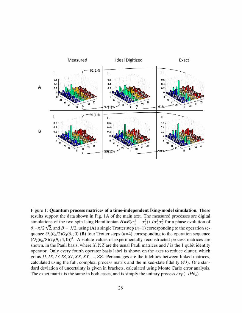
Figure 1: Quantum process matrices of a time-independent Ising-model simulation. Theseresults support the data shown in Fig. 1A of the main text. The measured processes are digitalsimulations of the two-spin Ising Hamiltonian H=B(σ1

z + σ2z )+Jσ1

xσ2x for a phase evolution of

θa=π/2√

2, and B = J/2, using (A) a single Trotter step (n=1) corresponding to the operation se-quence O2(θa/2)O4(θa, 0) (B) four Trotter steps (n=4) corresponding to the operation sequence(O2(θa/8)O4(θa/4, 0))4. Absolute values of experimentally reconstructed process matrices areshown, in the Pauli basis, where X,Y,Z are the usual Pauli matrices and I is the 1 qubit identityoperator. Only every fourth operator basis label is shown on the axes to reduce clutter, whichgo as II, IX, IY, IZ, XI, XX, XY, ....,ZZ. Percentages are the fidelities between linked matrices,calculated using the full, complex, process matrix and the mixed-state fidelity (43). One stan-dard deviation of uncertainty is given in brackets, calculated using Monte Carlo error analysis.The exact matrix is the same in both cases, and is simply the unitary process exp(−iHθa).

28

Figure 2: Digital simulation of a time-dependent Ising model. These results support the datashown in Fig. 1B of the main text. (A) A linearly increasing spin-spin interaction strength (overa total phase π/2) is discretised into 8 digital steps. Each step of the simulation is built from fixedsized operational building blocks, as shown. (B) The initial state | ↑↑〉x evolves into an entangledsuperposition of the states | →→〉 and | ←←〉x, which is a close approximation of the groundstate of the final Hamiltonian. Black percentages are measured fidelities between the measuredand ideal digitised states, quantified by the mixed-state fidelity (43). Green percentages quantifythe measured entanglement by its tangle (27). Both are derived from full state reconstructions,shown in (D). Uncertainties in these values of 1 standard deviation, derived from a Monte Carlosimulation based on the experimentally obtained density matrices, are determined for steps 0 to8 to be (1, 1, 1, 2, 1, 1, 2, 1, 2)% for the overlap with the ideally digitised state and (1, 1, 2, 4, 5,3, 5, 4, 6)% for the tangle, respectively. (C) Operation sequence of the digital simulation. (D)Experimentally reconstructed density matrices at each of the 8 digital steps in the simulation(including the initial state at step 0).

29

Figure 3: First and second-order digital simulations of a two-spin Ising model. The graphicin the top right corner of each panel shows the operational sequence for a single digital timestep. Dynamics of the initial state | →→〉x using (A) first and (B) second order Trotter-Suzikiapproximations. D=O4(π/8, 0), C=O2(π/8), C/2=O2(π/16), and B = J. The initial spin state iscreated starting from | ↓↓〉 and applying an O3(π/4, π/2) operation.

30

Figure 4: Quantum process matrices of Ising, XY and XYZ simulations. Absolute valuesof experimentally reconstructed process matrices are shown, in the Pauli basis, where X,Y,Zare the usual Pauli matrices and I is the 1 qubit identity operator. Only every fourth operatorbasis label is shown on the axis to reduce clutter, which go as II, IX, IY, IZ, XI, XX, XY, ....,ZZ.Percentages are the process fidelities between linked matrices (mixed-state fidelity (43)). Onestandard deviation of uncertainty is given in brackets, calculated using Monte Carlo error anal-ysis. The number of fundamental operations implemented for the simulations characterised are8, 16 and 28 for the Ising, XY and XYZ respectively.

31

Figure 5: Digital simulations of long-range Ising model. A single digital time step in eachcase is C.D=O2(Bπ/16, π).D=O4(π/16, 0). (— Exact, Ideal Digital, /_ Data). (A) 3 spincase for J/B=2 (A) i. is the same as Fig.3A in the main text. (B) 3 spin case for J/B=0.5 suchthat the transverse field is dominant. (C) 4 spin case for J/B=2. (C) i. is the same as Fig.4Ain the main text. (D). i. Energy level diagram of the 4-spin Hamiltonian simulated in panel C.The initial state | ↓↓↓↓〉 is a superposition of 3 of the different energy eigenstates, highlighted inred and with probabilities given as percentages (unpopulated energy levels are shown in grey).ii. Fourier transform of the black data trace in panel (C) i. clearly resolving the energy gap E2.The dashed red trace is the Fourier transform of the exact dynamics after 4 times the evolutionwindow.

32

Figure 6: Engineering arbitrary spin-spin coupling distributions. Three spin simulationsof Ising models with unequal spin-spin coupling distributions. Results are presented in twocomplementary bases (— Exact, /N Data). The graphic in the top right corner of each panelshows the operational sequence for a single digital step. D=O4(π/16, π), E=O1(π/2, n), wheren is the qubit on which E is shown to operate in the graphic. (A) The coupling strength is twiceas large between spins 2 and 3 as any other pair. (A)i is the same as Fig. 3A in the main text.(B) Nearest-neighbour coupling. The first operation sequence D.E.D.E couples only spins 2and 3. The second sequence couples only spins 1 and 2. We note that the total simulated phaseevolution in (B) is less than in (A) simply because the number of pulses that can be stored inthe memory of our pulse generator had reached its default limit (150 phase coherent pulses).This could be increased with a small amount of work, but the dynamics can already be seento have significantly decayed by this point. While all terms commute in each Hamiltonian,a stroboscopic approach is used, as will be necessary in future simulations where additionalnon-commuting interactions are incorporated.

33

Figure 7: Digital simulations of a three-spin interaction with a transverse field. The uppergraphs compare exact and ideal-digitized dynamics, the lower graphs show measured results.(A) Zero transverse field. This reproduces the dynamics shown in Fig. 3C of the main text,but in a stroboscopic way i.e. rather than adjusting the phase of operation E to simulate thedynamics, the phase of E is fixed at π/4 and the sequence D.E.D is repeated for each data point.This is expensive in terms of the number of operations required, but essential if additionalnon-commuting interactions are to be simulated following a digital approach. (B) Non-zerotransverse field. In both cases the dynamics rapidly damp due to the large number of oper-ations for each digital step and subsequent decoherence. The graphic in the top right cornershows the operational sequence for a single digital time step. C=O3(Bπ/4, π), D=O4(π/4, 0),E=O1(π/4, 1).

34

Table 3: Measured output state fidelities after the 6-qubit operationU(π/4)=exp(−iσyσxσxσxσxσxπ/4), for the orthogonal set of input states shown. Ideallythese are eigenstates and should be unchanged by the operation. This table shows 32 of the 64states that form a complete basis. The other 32 are shown in Table IV. The average output statefidelity between both tables is F1=0.792(4).

Input Fidelity|+〉y|+++++〉x 0.78(3)|+〉y|++++−〉x 0.81(3)|+〉y|+++−+〉x 0.83(3)|+〉y|+++−−〉x 0.77(3)|+〉y|++−++〉x 0.78(3)|+〉y|++−+−〉x 0.75(3)|+〉y|++−−+〉x 0.75(3)|+〉y|++−−−〉x 0.80(3)|+〉y|+−+++〉x 0.76(3)|+〉y|+−++−〉x 0.79(3)|+〉y|+−+−+〉x 0.75(3)|+〉y|+−+−−〉x 0.71(3)|+〉y|+−−++〉x 0.74(3)|+〉y|+−−+−〉x 0.77(3)|+〉y|+−−−+〉x 0.87(2)|+〉y|+−−−−〉x 0.79(3)|+〉y|−++++〉x 0.77(3)|+〉y|−+++−〉x 0.86(2)|+〉y|−++−+〉x 0.79(3)|+〉y|−++−−〉x 0.73(3)|+〉y|−+−++〉x 0.78(3)|+〉y|−+−+−〉x 0.77(3)|+〉y|−+−−+〉x 0.83(3)|+〉y|−+−−−〉x 0.77(3)|+〉y|−−+++〉x 0.76(3)|+〉y|−−++−〉x 0.75(3)|+〉y|−−+−+〉x 0.89(2)|+〉y|−−+−−〉x 0.79(3)|+〉y|−−−++〉x 0.83(3)|+〉y|−−−+−〉x 0.81(3)|+〉y|−−−−+〉x 0.82(3)|+〉y|−−−−−〉x 0.80(3)

35

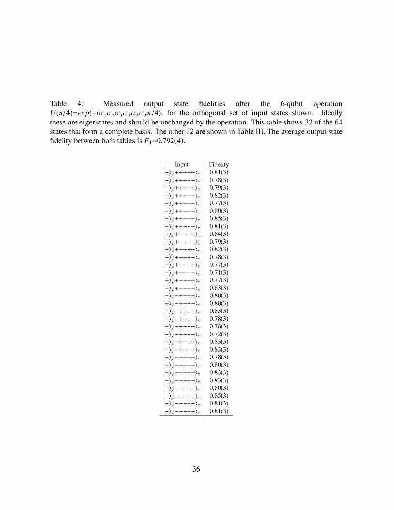
Table 4: Measured output state fidelities after the 6-qubit operationU(π/4)=exp(−iσyσxσxσxσxσxπ/4), for the orthogonal set of input states shown. Ideallythese are eigenstates and should be unchanged by the operation. This table shows 32 of the 64states that form a complete basis. The other 32 are shown in Table III. The average output statefidelity between both tables is F1=0.792(4).

Input Fidelity|−〉y|+++++〉x 0.81(3)|−〉y|++++−〉x 0.78(3)|−〉y|+++−+〉x 0.79(3)|−〉y|+++−−〉x 0.82(3)|−〉y|++−++〉x 0.77(3)|−〉y|++−+−〉x 0.80(3)|−〉y|++−−+〉x 0.85(3)|−〉y|++−−−〉x 0.81(3)|−〉y|+−+++〉x 0.84(3)|−〉y|+−++−〉x 0.79(3)|−〉y|+−+−+〉x 0.82(3)|−〉y|+−+−−〉x 0.78(3)|−〉y|+−−++〉x 0.77(3)|−〉y|+−−+−〉x 0.71(3)|−〉y|+−−−+〉x 0.77(3)|−〉y|+−−−−〉x 0.83(3)|−〉y|−++++〉x 0.80(3)|−〉y|−+++−〉x 0.80(3)|−〉y|−++−+〉x 0.83(3)|−〉y|−++−−〉x 0.78(3)|−〉y|−+−++〉x 0.78(3)|−〉y|−+−+−〉x 0.72(3)|−〉y|−+−−+〉x 0.83(3)|−〉y|−+−−−〉x 0.83(3)|−〉y|−−+++〉x 0.78(3)|−〉y|−−++−〉x 0.80(3)|−〉y|−−+−+〉x 0.83(3)|−〉y|−−+−−〉x 0.83(3)|−〉y|−−−++〉x 0.80(3)|−〉y|−−−+−〉x 0.85(3)|−〉y|−−−−+〉x 0.81(3)|−〉y|−−−−−〉x 0.81(3)

36

Table 5: Measured output state fidelities after the 6-qubit operationU(π/4)=exp(−iσyσxσxσxσxσxπ/4), for the orthogonal set of input states shown. Ideallythese should become entangled states. Fidelities are derived from 6 parity measurements andtwo logical populations (extracted from one measurement in the logical basis). This tableshows 32 of the 64 states that form a complete basis. The other 32 are shown in Table VI. Theaverage output state fidelity between both tables is F1=0.767(6). Ideally the populations shouldeach be 0.5 and the absolute value of each parity should be 1.

Input Parity Populations Fidelity1 2 3 4 5 6 1 2

|000000〉 0.64(8) -0.64(8) 0.62(8) -0.62(8) 0.64(8) -0.66(8) 0.34(5) 0.45(5) 0.71(5)|000001〉 0.74(7) -0.64(8) 0.80(6) -0.58(8) 0.86(5) -0.66(8) 0.33(5) 0.51(5) 0.78(5)|000010〉 0.76(6) -0.76(6) 0.74(7) -0.72(7) 0.74(7) -0.76(6) 0.46(5) 0.38(5) 0.79(5)|000011〉 0.84(5) -0.74(7) 0.66(8) -0.78(6) 0.76(6) -0.80(6) 0.35(5) 0.46(5) 0.79(5)|000100〉 0.72(7) -0.66(8) 0.68(7) -0.68(7) 0.72(7) -0.76(6) 0.32(5) 0.46(5) 0.74(5)|000101〉 0.68(7) -0.72(7) 0.86(5) -0.86(5) 0.72(7) -0.76(6) 0.41(5) 0.37(5) 0.77(5)|000110〉 0.84(5) -0.80(6) 0.86(5) -0.80(6) 0.74(7) -0.88(5) 0.43(5) 0.38(5) 0.82(5)|000111〉 0.88(5) -0.68(7) 0.72(7) -0.82(6) 0.70(7) -0.82(6) 0.35(5) 0.46(5) 0.79(5)|001000〉 0.80(6) -0.64(8) 0.54(8) -0.76(6) 0.70(7) -0.72(7) 0.46(5) 0.39(5) 0.77(5)|001001〉 0.84(5) -0.66(8) 0.68(7) -0.68(7) 0.82(6) -0.76(6) 0.37(5) 0.42(5) 0.76(5)|001010〉 0.84(5) -0.72(7) 0.72(7) -0.80(6) 0.62(8) -0.74(7) 0.43(5) 0.39(5) 0.78(5)|001011〉 0.84(5) -0.58(8) 0.68(7) -0.80(6) 0.70(7) -0.78(6) 0.37(5) 0.48(5) 0.79(5)|001100〉 0.80(6) -0.72(7) 0.76(6) -0.82(6) 0.64(8) -0.86(5) 0.46(5) 0.37(5) 0.80(5)|001101〉 0.74(7) -0.76(6) 0.86(5) -0.72(7) 0.70(7) -0.86(5) 0.39(5) 0.44(5) 0.80(5)|001110〉 0.82(6) -0.74(7) 0.86(5) -0.80(6) 0.76(6) -0.82(6) 0.51(5) 0.28(4) 0.80(5)|001111〉 0.88(5) -0.64(8) 0.52(9) -0.74(7) 0.72(7) -0.76(6) 0.28(4) 0.55(5) 0.77(5)|010000〉 0.88(5) -0.72(7) 0.74(7) -0.74(7) 0.74(7) -0.84(5) 0.44(5) 0.38(5) 0.80(5)|010001〉 0.76(6) -0.74(7) 0.66(8) -0.80(6) 0.78(6) -0.84(5) 0.36(5) 0.41(5) 0.77(5)|010010〉 0.84(5) -0.68(7) 0.88(5) -0.76(6) 0.72(7) -0.60(8) 0.40(5) 0.48(5) 0.81(5)|010011〉 0.76(6) -0.64(8) 0.78(6) -0.62(8) 0.80(6) -0.76(6) 0.36(5) 0.46(5) 0.77(5)|010100〉 0.88(5) -0.78(6) 0.76(6) -0.82(6) 0.78(6) -0.80(6) 0.45(5) 0.45(5) 0.85(5)|010101〉 0.78(6) -0.84(5) 0.72(7) -0.78(6) 0.76(6) -0.86(5) 0.28(4) 0.46(5) 0.77(5)|010110〉 0.86(5) -0.86(5) 0.82(6) -0.92(4) 0.84(5) -0.82(6) 0.45(5) 0.42(5) 0.86(5)|010111〉 0.82(6) -0.80(6) 0.78(6) -0.72(7) 0.72(7) -0.76(6) 0.23(4) 0.56(5) 0.78(5)|011000〉 0.76(6) -0.72(7) 0.80(6) -0.78(6) 0.74(7) -0.86(5) 0.38(5) 0.50(5) 0.83(5)|011001〉 0.86(5) -0.72(7) 0.78(6) -0.76(6) 0.72(7) -0.80(6) 0.33(5) 0.43(5) 0.77(5)|011010〉 0.80(6) -0.74(7) 0.68(7) -0.76(6) 0.78(6) -0.90(4) 0.49(5) 0.37(5) 0.82(5)|011011〉 0.78(6) -0.80(6) 0.56(8) -0.56(8) 0.66(8) -0.70(7) 0.29(5) 0.50(5) 0.73(5)|011100〉 0.84(5) -0.82(6) 0.76(6) -0.68(7) 0.72(7) -0.78(6) 0.48(5) 0.37(5) 0.81(5)|011101〉 0.82(6) -0.76(6) 0.46(9) -0.42(9) 0.40(9) -0.64(8) 0.31(5) 0.45(5) 0.67(5)|011110〉 0.90(4) -0.68(7) 0.76(6) -0.70(7) 0.66(8) -0.80(6) 0.50(5) 0.33(5) 0.79(5)|011111〉 0.64(8) -0.58(8) 0.64(8) -0.68(7) 0.70(7) -0.74(7) 0.26(4) 0.57(5) 0.75(5)

37

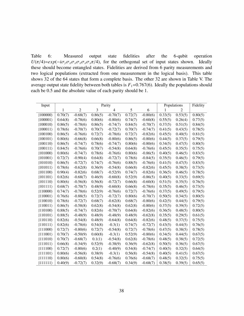
Table 6: Measured output state fidelities after the 6-qubit operationU(π/4)=exp(−iσyσxσxσxσxσxπ/4), for the orthogonal set of input states shown. Ideallythese should become entangled states. Fidelities are derived from 6 parity measurements andtwo logical populations (extracted from one measurement in the logical basis). This tableshows 32 of the 64 states that form a complete basis. The other 32 are shown in Table V. Theaverage output state fidelity between both tables is F1=0.767(6). Ideally the populations shouldeach be 0.5 and the absolute value of each parity should be 1.

Input Parity Populations Fidelity1 2 3 4 5 6 1 2

|100000〉 0.70(7) -0.68(7) 0.86(5) -0.70(7) 0.72(7) -0.80(6) 0.33(5) 0.53(5) 0.80(5)|100001〉 0.64(8) -0.78(6) 0.80(6) -0.80(6) 0.74(7) -0.60(8) 0.55(5) 0.26(4) 0.77(5)|100010〉 0.86(5) -0.78(6) 0.86(5) -0.74(7) 0.84(5) -0.70(7) 0.37(5) 0.51(5) 0.84(5)|100011〉 0.78(6) -0.70(7) 0.70(7) -0.72(7) 0.70(7) -0.74(7) 0.41(5) 0.43(5) 0.78(5)|100100〉 0.86(5) -0.76(6) 0.72(7) -0.78(6) 0.72(7) -0.82(6) 0.45(5) 0.40(5) 0.81(5)|100101〉 0.80(6) -0.66(8) 0.66(8) -0.80(6) 0.86(5) -0.80(6) 0.44(5) 0.37(5) 0.79(5)|100110〉 0.86(5) -0.74(7) 0.78(6) -0.74(7) 0.80(6) -0.80(6) 0.34(5) 0.47(5) 0.80(5)|100111〉 0.84(5) -0.76(6) 0.70(7) -0.54(8) 0.64(8) -0.76(6) 0.45(5) 0.35(5) 0.75(5)|101000〉 0.80(6) -0.74(7) 0.78(6) -0.76(6) 0.80(6) -0.86(5) 0.40(5) 0.46(5) 0.83(5)|101001〉 0.72(7) -0.90(4) 0.64(8) -0.72(7) 0.78(6) -0.84(5) 0.35(5) 0.46(5) 0.79(5)|101010〉 0.86(5) -0.72(7) 0.74(7) -0.76(6) 0.88(5) -0.76(6) 0.41(5) 0.47(5) 0.83(5)|101011〉 0.78(6) -0.62(8) 0.36(9) -0.54(8) 0.66(8) -0.82(6) 0.45(5) 0.38(5) 0.73(5)|101100〉 0.90(4) -0.82(6) 0.68(7) -0.52(9) 0.74(7) -0.82(6) 0.36(5) 0.46(5) 0.78(5)|101101〉 0.82(6) -0.68(7) 0.46(9) -0.60(8) 0.52(9) -0.86(5) 0.40(5) 0.33(5) 0.69(5)|101110〉 0.80(6) -0.56(8) 0.56(8) -0.72(7) 0.66(8) -0.60(8) 0.51(5) 0.35(5) 0.76(5)|101111〉 0.68(7) -0.70(7) 0.48(9) -0.60(8) 0.66(8) -0.78(6) 0.35(5) 0.46(5) 0.73(5)|110000〉 0.74(7) -0.78(6) 0.52(9) -0.76(6) 0.72(7) -0.76(6) 0.37(5) 0.49(5) 0.79(5)|110001〉 0.76(6) -0.88(5) 0.72(7) -0.72(7) 0.80(6) -0.70(7) 0.50(5) 0.34(5) 0.80(5)|110010〉 0.78(6) -0.72(7) 0.68(7) -0.62(8) 0.68(7) -0.80(6) 0.42(5) 0.44(5) 0.79(5)|110011〉 0.86(5) -0.58(8) 0.62(8) -0.54(8) 0.62(8) -0.80(6) 0.37(5) 0.39(5) 0.72(5)|110100〉 0.88(5) -0.74(7) 0.82(6) -0.70(7) 0.64(8) -0.82(6) 0.36(5) 0.48(5) 0.80(5)|110101〉 0.88(5) -0.48(9) 0.48(9) -0.48(9) 0.48(9) -0.62(8) 0.35(5) 0.29(5) 0.61(5)|110110〉 0.82(6) -0.54(8) 0.48(9) -0.64(8) 0.64(8) -0.82(6) 0.48(5) 0.37(5) 0.75(5)|110111〉 0.82(6) -0.78(6) 0.54(8) -0.3(1) 0.74(7) -0.72(7) 0.43(5) 0.44(5) 0.76(5)|111000〉 0.72(7) -0.80(6) 0.72(7) -0.54(8) 0.72(7) -0.78(6) 0.47(5) 0.38(5) 0.78(5)|111001〉 0.70(7) -0.50(9) 0.60(8) -0.3(1) 0.52(9) -0.80(6) 0.34(5) 0.44(5) 0.67(5)|111010〉 0.70(7) -0.68(7) 0.1(1) -0.54(8) 0.62(8) -0.78(6) 0.48(5) 0.38(5) 0.72(5)|111011〉 0.66(8) -0.34(9) 0.52(9) -0.38(9) 0.36(9) -0.62(8) 0.50(5) 0.36(5) 0.67(5)|111100〉 0.72(7) -0.80(6) 0.2(1) -0.40(9) 0.54(8) -0.74(7) 0.40(5) 0.32(5) 0.64(5)|111101〉 0.80(6) -0.56(8) 0.38(9) -0.3(1) 0.56(8) -0.54(8) 0.40(5) 0.41(5) 0.67(5)|111110〉 0.80(6) -0.60(8) 0.54(8) -0.76(6) 0.76(6) -0.68(7) 0.48(5) 0.32(5) 0.75(5)|111111〉 0.40(9) -0.72(7) 0.32(9) -0.68(7) 0.34(9) -0.68(7) 0.38(5) 0.39(5) 0.65(5)

38

Figure 8: Effect of laser-ion coupling strength fluctuations. In each panel simulation resultsfrom a two-spin Ising model are compared with a theoretical model that incorporates increas-ing amounts of fluctuations in laser-ion coupling strength Ω. (A) dΩ/Ω=0% (B) 1% (C) 2%.Dashed lines; predicted results from model. Filled shapes; data. (↑↑ _↓↓)

39

Figure 9: Sensitivity of the simulations to imperfectly set operations. Simulation results of athree-spin Ising model (shown in Fig. 3A, main text) are compared with theoretical predictionsfor the cases of (A) ideal gate operations (B) non-ideal gate operations: the phase θ of the O4

operation used to simulate the spin-spin interaction in each digital step is wrong by 1%. Thefrequency mismatch in the previous panel is now largely corrected.

40

References and Notes

1. R. P. Feynman, Int. J. Theor. Phys. 21, 467 (1982).

2. I. Buluta, F. Nori, Science 326, 108 (2009).

3. S. Somaroo, C. H. Tseng, T. F. Havel, R. Laflamme, D. G. Cory, Phys. Rev. Lett. 82, 5381

(1999).

4. M. Greiner, O. Mandel, T. Esslinger, T. W. Hansch, I. Bloch, Nature 415, 39 (2002).

5. D. Leibfried, et al., Phys. Rev. Lett. 89, 247901 (2002).

6. A. Friedenauer, H. Schmitz, J. T. Glueckert, D. Porras, T. Schaetz, Nature Phys. 4, 757

(2008).

7. R. Gerritsma, et al., Nature 463, 68 (2010).

8. K. Kim, et al., Nature 465, 590 (2010).

9. B. P. Lanyon, et al., Nature Chem. 2, 106 (2010).

10. K. R. Brown, R. J. Clark, I. L. Chuang, Phys. Rev. Lett. 97, 050504 (2006).

11. J. T. Barreiro, et al., Nature 470, 486 (2011).

12. J. Simon, et al., Nature 472, 307 (2011).

13. S. Lloyd, Science 273, 1073 (1996).

14. E. Jane, G. Vidal, W. Dur, P. Zoller, J. I. Cirac, QUANTUM INFORMATION & COMPU-

TATION 3, 15 (2003).

41

15. N. Wiebe, D. W. Berry, P. Hoyer, B. C. Sanders, Simulating quantum dynamics on a quan-

tum computer, http://arxiv.org/abs/1011.3489 (2010).

16. M. Nielsen, I. Chuang, Quantum Computation and Quantum Information (Cambridge Uni-

versity Press, 2001).

17. A. Steane, Nature 399, 124 (1999).

18. A. Auerbach, Interacting Electrons and Quantum Magnetism (Springer-Verlag New York,

1994).

19. P. Schindler, et al., Science 332, 1059 (2011).

20. H. F. Trotter, Proc. Amer. Math. Soc. 10, 545 (1959).

21. S. Lloyd, L. Viola, Phys. Rev. A 65, 010101 (2001).

22. Materials and methods are available as supplementary online material.

23. A. Sørensen, K. Mølmer, Phys. Rev. Lett. 82, 1971 (1999).

24. J. Benhelm, G. Kirchmair, C. F. Roos, R. Blatt, Nature Physics 4, 463 (2008).

25. D. Porras, J. I. Cirac, Phys. Rev. Lett. 92, 207901 (2004).

26. J. F. Poyatos, J. I. Cirac, P. Zoller, Phys. Rev. Lett. 78, 390 (1997).

27. A. G. White, et al., J. Opt. Soc. Am. B 24, 172 (2007).

28. W. Dur, G. Vidal, J. I. Cirac, Phys. Rev. A 62, 062314 (2000).

29. I. Kassal, J. D. Whitfield, A. Perdomo-Ortiz, M.-H. Yung, A. Aspuru-Guzik, Annual Review

of Physical Chemistry 62, 185 (2011).

42

30. C. Nayak, S. H. Simon, A. Stern, M. Freedman, S. Das Sarma, Rev. Mod. Phys. 80, 1083

(2008).

31. H. F. Hofmann, Phys. Rev. Lett. 94, 160504 (2005).

32. T. Monz, et al., Phys. Rev. Lett. 102, 040501 (2009).

33. A. Gilchrist, N. K. Langford, M. A. Nielsen, Phys. Rev. A. 71, 062310 (2005).

34. J. P. Home, et al., Science 325, 1227 (2009).

35. G. Kirchmair, Quantum non-demolition measurements and quantum simulation, Ph.D. the-

sis, Leopold Franzens University of Innsbruck, http://heart-c704.uibk.ac.at/ (2010).

36. C. F. Roos, New J. Phys. 10, 013002 (2008).

37. V. Nebendahl, H. Haffner, C. F. Roos, Phys. Rev. A 79, 012312 (2009).

38. M. Riebe, et al., Phys. Rev. Lett. 97, 220407 (2006).

39. M. Suzuki, Physics Letters A 180, 232 (1993).

40. M. Mueller, K. Hammerer, Y. L. Zhou, C. F. Roos, P. Zoller, Simulating open quantum sys-

tems: from many-body interactions to stabilizer pumping, http://arxiv.org/abs/1104.2507.

41. T. Monz, et al., Phys. Rev. Lett. 106, 130506 (2011).

42. G. Kirchmair, et al., New J. Phys. 11, 023002 (2009).

43. R. Jozsa, Journal of Modern Optics 41, 2315 (1994).

43