�������� � ��� � ���� ��������

Introduction

Stability of a power system is its ability to return to normal or stable operating

conditions after having been subjected to some form of disturbance.

Conversely, instability means a condition denoting loss of synchronism or

falling out of step.

Though stability of a power system is a single phenomenon, for the purpose of

analysis, it is classified as Steady State Analysis and Transient Stability. analysis, it is classified as Steady State Analysis and Transient Stability.

Increase in load is a kind of disturbance. If increase in loading takes place

gradually and in small steps and the system withstands this change and

performs satisfactorily, then the system is said to be in STADY STATE

STABILITY. Thus the study of steady steady state stability is basically

concerned with the determination of upper limit of machine’s loading before

losing synchronism, provided the loading is increased gradually at a slow rate.

In practice, load change may not be gradual. Further, there may be sudden

disturbances due to

i) Sudden change of load

ii) Switching operation

iii) Loss of generation

iv) Fault

Following such sudden disturbances in the power system, rotor speeds, rotor Following such sudden disturbances in the power system, rotor speeds, rotor

angular differences and power transfer undergo fast changes whose

magnitudes are dependent upon the severity of disturbances, For a large

disturbance, changes in angular differences may be so large as to cause the

machine to fall out of step. This type of instability is known as TRANSIENT

INSTABILITY. Transient stability is a fast phenomenon, usually occurring

within one second for a generator close to the cause of disturbance.

Short circuit is a severe type of disturbance. During a fault, electrical powers

from the nearby generators are reduced drastically, while powers from remote

generators are scarily affected. In some cases, the system may be stable even

with sustained fault; whereas in other cases system will be stable only if the

fault is cleared with sufficient rapidity. Whether the system is stable on the

occurrence of a fault depends not only on the system itself, but also on the

type of fault, location of fault, clearing time and the method of clearing.

Transient stability limit is almost always lower than the steady state limit and

hence it is much important. Transient stability limit depends on the type of

disturbance, location and magnitude of disturbance.

Review of mechanics

Transient stability analysis involves some mechanical properties of the

machines in the system. After every disturbance, the machines must adjust

the relative angles of their rotors to meet the condition of the power transfer

involved. The problem is mechanical as well as electrical.

The kinetic energy of an electric machine is given by

K.E. = 2�

1 I Mega Joules (1) K.E. = 2�

21 I Mega Joules (1)

where I is the Moment of Inertia in Mega Joules sec.2 / elec. deg.2

� is the angular velocity in elec. deg. / sec.

Angular Momentum M = I �; Then from eqn. (1), K.E. can be written as

K.E. = �M21 Mega Joules (2)

The angular momentum M depends on the size of the machine as well as on its

type.

The Inertia constant H is defined as the Mega Joules of stored energy of the

machine at synchronous speed per MVA of the machine. When so defined, the

relation between the Angular Momentum M and the Inertia constant H can be

derived as follows.

Relationship between M and H

By definition H = MVAinratingsMachine'MJinenergyStored

Let G be the rating of the machine in MVA. Then

Stored energy = G H MJ (3)

Further, K.E. = �M21 MJ = M

21 (2 � f) MJ = M x � f MJ (4)

Stored energy = G H MJ (3)

Further, K.E. = �M21 MJ = M

21 (2 � f) MJ = M x � f MJ (4)

From eqns. (3) and (4), we get

G H = M x � f; Thus

M = f�

HG MJ sec. / elec. rad. (5)

When the angles are measured in elec. deg.

M = f180

HG MJ sec. / elec. deg. (6)

While the angular momentum M depend on the size of the machine as well as

on its type, inertia constant H does not vary very much with the size of the

machine, The quantity H has a relatively narrow range of values for each class

of machine.

Swing equation

The differential equation that relates the angular momentum M, the

acceleration power Pa and the rotor angle � is known as SWING EQUATION.

Solution of swing equation will show how the rotor angle changes with respect

to time following a disturbance. The plot of � Vs t is called the SWING CURVE.

Once the swing curve is known, the stability of the system can be assessed.

The flow of mechanical and electrical power in a generator and motor are

shown in Fig. 1.

Pe

Ts

Pe Te � �

Consider the generator shown in Fig. 1(a). It receives mechanical power Pm at

the shaft torque Ts and the angular speed � via. shaft from the prime-mover. It

delivers electrical power Pe to the power system network via. the bus bars. The

generator develops electromechanical torque Te in opposition to the shaft

torque Ts. At steady state, Ts = Te. Assuming that the windage and the friction

torque are negligible, the accelerating torque acting on the rotor is given by

Ta = Ts – Te (7)

Te �

Pm � Ts

�

�Pm

Generator

�

�

Motor

(b) (a) Fig. 1

Ta = Ts – Te (7)

Multiplying by � on both sides, we get

Pa = Ps – Pe (8)

In case of motor

Ta = Te – Ts (9)

Pa = Pe – Ps (10)

In general, the accelerating power is given by

Pa = Input Power – Output Power (11) Pa = Input Power – Output Power (11)

We know that Pa = Ta � = I � � = M � = M 2

2

dt�d

Thus M 2

2

dt�d = Pa (12)

Here �= angular displacement (radians)

� = dtd� = angular velocity (rad. / sec.); � =

dtd� = 2

2

dt�d = angular acceleration

Now we can see how the angular displacement � can be related to the rotor

angle �.

Consider an object moving at a linear speed of vs ± �v. It is required to find its

displacement at any time t. For this purpose, introduce another object moving

with a constant speed of vs. Then, at any time t, the displacement of the first

object is given by

x = vs t + d

where d is the displacement of the first object with respect to the second as

shown in Fig. 2.

vs + �v

x

d

Similarly in the case of angular movement, the angular displacement � , at any

time t is given by

� = �s t + � (13)

where � is the angular displacement of the rotor from synchronously rotating

reference axis, rotating at synchronous speed �s. The angle � is also called as

LOAD ANGLE or TORQUE ANGLE.

vs d

Fig. 2

In view of eqn.(13) � = �s t + �

dtd� = �s +

dtd� (14)

2

2

dt�d = 2

2

dt�d (15)

From equations (12) and (15), we get

M 2

2

dt�d

= Pa (16)

The above equation is known as SWING EQUATION.

In case damping power is to be included, then eqn.(16) gets modified as

M 2

2

dt�d

+ D dtd� = Pa (17)

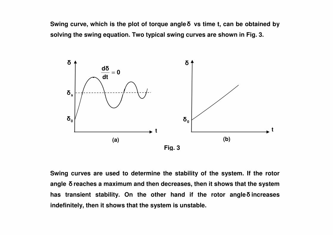
Swing curve, which is the plot of torque angle� vs time t, can be obtained by

solving the swing equation. Two typical swing curves are shown in Fig. 3.

�

s�

�

�

�

. 0dtd� =

Swing curves are used to determine the stability of the system. If the rotor

angle � reaches a maximum and then decreases, then it shows that the system

has transient stability. On the other hand if the rotor angle� increases

indefinitely, then it shows that the system is unstable.

t t

0� 0�

(a) (b)

Fig. 3

We are going to study the stability of (1) a generator connected to infinite bus

and (2) a synchronous motor drawing power from infinite bus.

We know that the complex power is given by

P + j Q = V I * i.e. P – j Q = V * I Thus real power P = Re {V * I}

Consider a generator connected to infinite bus.

V is the voltage at infinite bus.

Taking this as ref. V = 00V ∠

E is internal voltage of generator.

��

I V E

Xd XT

E – j X I = V i.e. E = V + j X I

Internal voltage E leads V; Thus E = �E ∠

Current I = ]V�sinEj�cosE[Xj1 −+

Electric output power Pe = Re [ IV ] = �sinX

VE = Pmax sin �

E is internal voltage of generator.

X is the total reactance

I V E

E

� V

I

Consider a synchronous motor drawing power from infinite bus.

V – j X I = E

Thus E = �E −∠ Current I = )]�sinEj�cosE(V[Xj1 −−

I I

��

V E

Xd XT

E

� V

Electric input power Pe = Re [ IV ] = �sinX

VE = Pmax sin �

Thus Swing equation for alternator is M 2

2

dt�d

= Pm – Pmax sin �

Swing equation for motor is M 2

2

dt�d

= Pmax sin � - Pm

Notice that the swing equation is second order nonlinear differential equation

Equal area criterion

The accelerating power in swing equation will have sine term. Therefore the

swing equation is non-linear differential equation and obtaining its solution is

not simple. For two machine system and one machine connected to infinite

bus bar, it is possible to say whether a system has transient stability or not,

without solving the swing equation. Such criteria which decides the stability,

makes use of equal area in power angle diagram and hence it is known as

EQUAL AREA CRITERION. Thus the principle by which stability under

transient conditions is determined without solving the swing equation, but transient conditions is determined without solving the swing equation, but

makes use of areas in power angle diagram, is called the EQUAL AREA

CRITERION.

From the Fig. 3, it is clear that if the rotor angle � oscillates, then the system is

stable. For � to oscillate, it should reach a maximum value and then should

decrease. At that point dtd� = 0. Because of damping inherently present in the

system, subsequence oscillations will be smaller and smaller. Thus while �

changes, if dtd� = 0, then the stability is ensured.

The swing equation for the alternator connected to the infinite bus bars is

M 2

2

dt�d

= Ps – Pe (18)

Multiplying both sides by dtd� , we get

M 2

2

dt�d

dtd� = (Ps – Pe)

dtd� i.e.

=2)d�

(d

M1 (Ps – Pe)

d� (19) =2)dtd�

(dtd

M21 (Ps – Pe)

dtd� (19)

Thus M

)P(P2d�dt

)dtd�

(dtd es2 −

= ; i.e. M

)P(P2)

dtd�

(d�d es2 −

=

On integration 2

dtd�

)( = �−δ

δ0M

d�)P(P2 es i.e.

dtd� = �

−�

�

es

0M

d�)P(P2 (20)

dtd� = �

−�

�

es

0M

d�)P(P2

Before the disturbance occurs, 0� was the torque angle. At that time dtd� = 0.

Once the disturbance occurs, dtd� is no longer zero and � starts changing.

Torque angle �will cease to change and the machine will again be operating at

synchronous speed after a disturbance, when dtd� = 0 or when

−δ )P(P2 δ

(20)

�−δ

δ0

d�M

)P(P2 es = 0 i.e. � −δ

δ0

d�)P(P es = 0 (21)

If there exist a torque angle � for which the above is satisfied, then the

machine will attain a new operating point and hence it has transient stability.

The machine will not remain at rest with respect to infinite bus at the first time

when dtd� = 0. But due to damping present in the system, during subsequent

oscillation, maximum value of � keeps on decreasing. Therefore, the fact that

� has momentarily stopped changing may be taken to indicate stability.

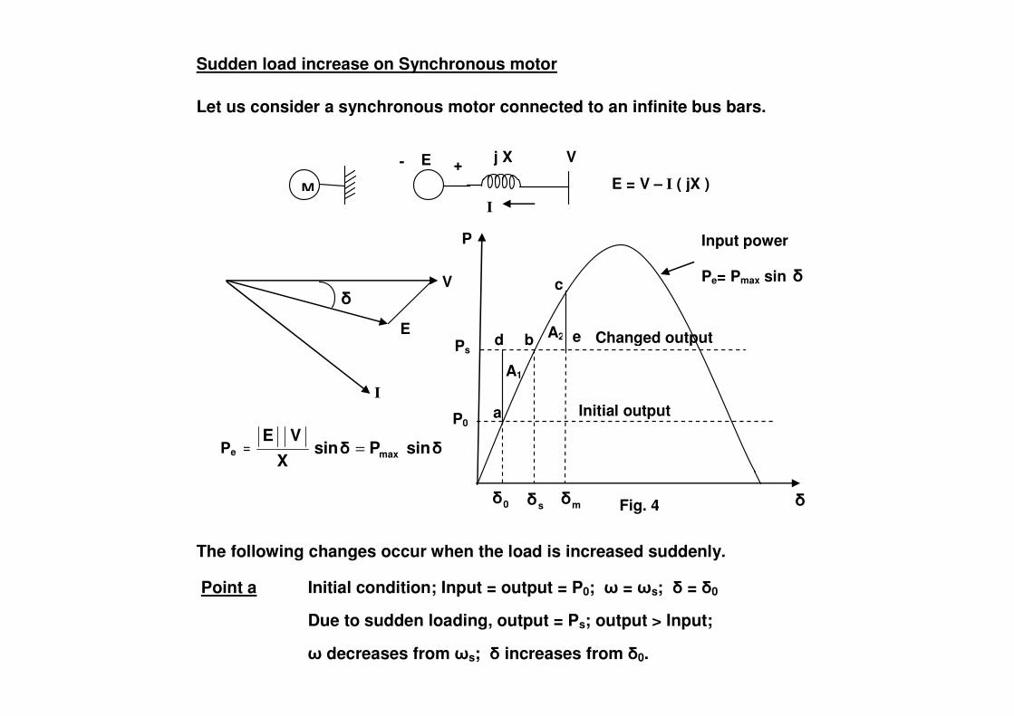
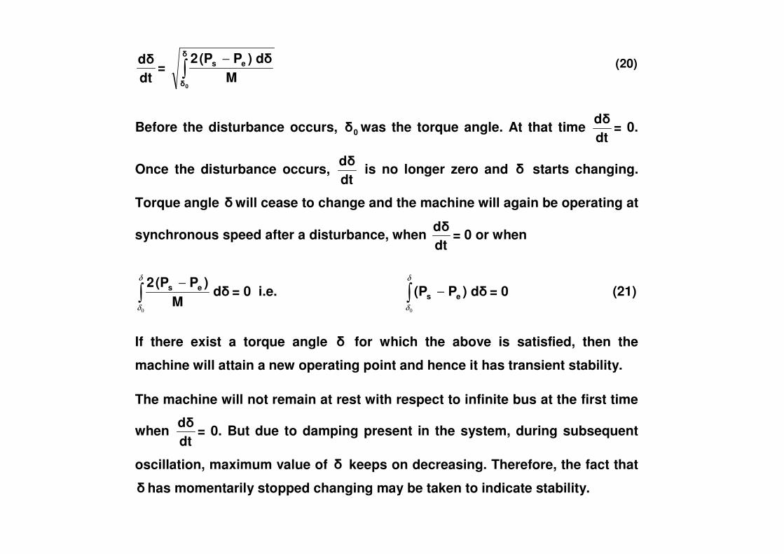
Sudden load increase on Synchronous motor

Let us consider a synchronous motor connected to an infinite bus bars.

I

j X E -

�� � E = V – I ( jX ) + V

� V

E

Input power

Pe= Pmax sin �

A2 Changed output e d

c

b

P

Ps

The following changes occur when the load is increased suddenly.

Point a Initial condition; Input = output = P0; � = �s; � = �0

Due to sudden loading, output = Ps; output > Input;

� decreases from �s; � increases from �0.

I

Pe���� �sinP�sinX

VEmax=

A1

m�

Initial output a

s�

0� �

P0

Fig. 4

�

�

�

�

�

�

�

�

�

�

� V

E

I

Pe���� �sinP�sinX

VEmax=

Input power

Pe= Pmax sin �

A2

A1

m�

Changed output

Initial output

e d

c

b

a

s�0� �

P

P0

Ps

Fig. 4 �

Between a-b Output > Input; Deceleration; � decreases; � increases.

Point b Output = Input; � = �min which is less than �s; � = �s

Since � is less than �s, � continues to increase.

Between b-c Input > output; Rotating masses start gaining energy;

Acceleration; � starts increasing from minimum value but still

less than �s; � continues to increase.

Point c Input > output; � = �s; � = �m; There is acceleration; � is

going to increase from �s; hence � is going to decrease from

�m.

m� s�

0� � Fig. 4

�

�

�

�

�

�

�

�

�

� V

E

I

Pe���� �sinP�sinX

VEmax=

Input power

Pe= Pmax sin �

A2

A1

Changed output

Initial output

e d

c

b

a

P

P0

Ps

�

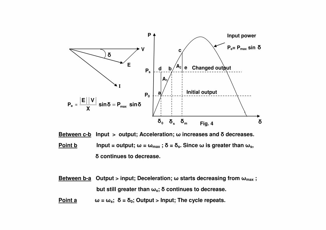
Between c-b Input > output; Acceleration; � increases and � decreases.

Point b Input = output; � = �max ; � = �s. Since � is greater than �s,

� continues to decrease.

Between b-a Output > input; Deceleration; � starts decreasing from �max ;

but still greater than �s; � continues to decrease.

Point a � = �s; � = �0; Output > Input; The cycle repeats.

�

m� s�

0� � Fig. 4

Because of damping present in the system, subsequent oscillations become

smaller and smaller and finally b will be the steady state operating point.

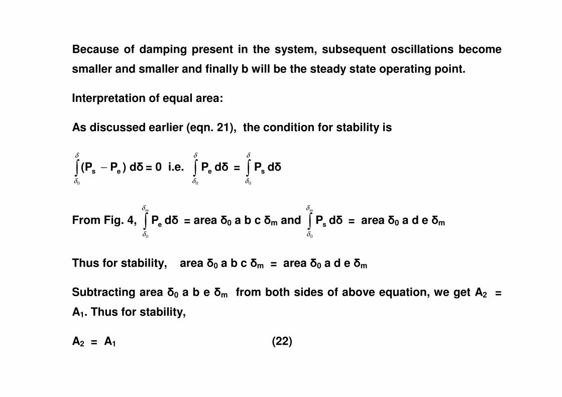
Interpretation of equal area:

As discussed earlier (eqn. 21), the condition for stability is

� −δ

δ0

d�)P(P es = 0 i.e. �δ

δ0

d�Pe = �δ

δ0

d�Ps

From Fig. 4, �mδ

δ0

d�Pe = area �0 a b c �m and �mδ

δ0

d�Ps = area �0 a d e �m

Thus for stability, area �0 a b c �m = area �0 a d e �m

Subtracting area �0 a b e �m from both sides of above equation, we get A2 =

A1. Thus for stability,

A2 = A1 (22)

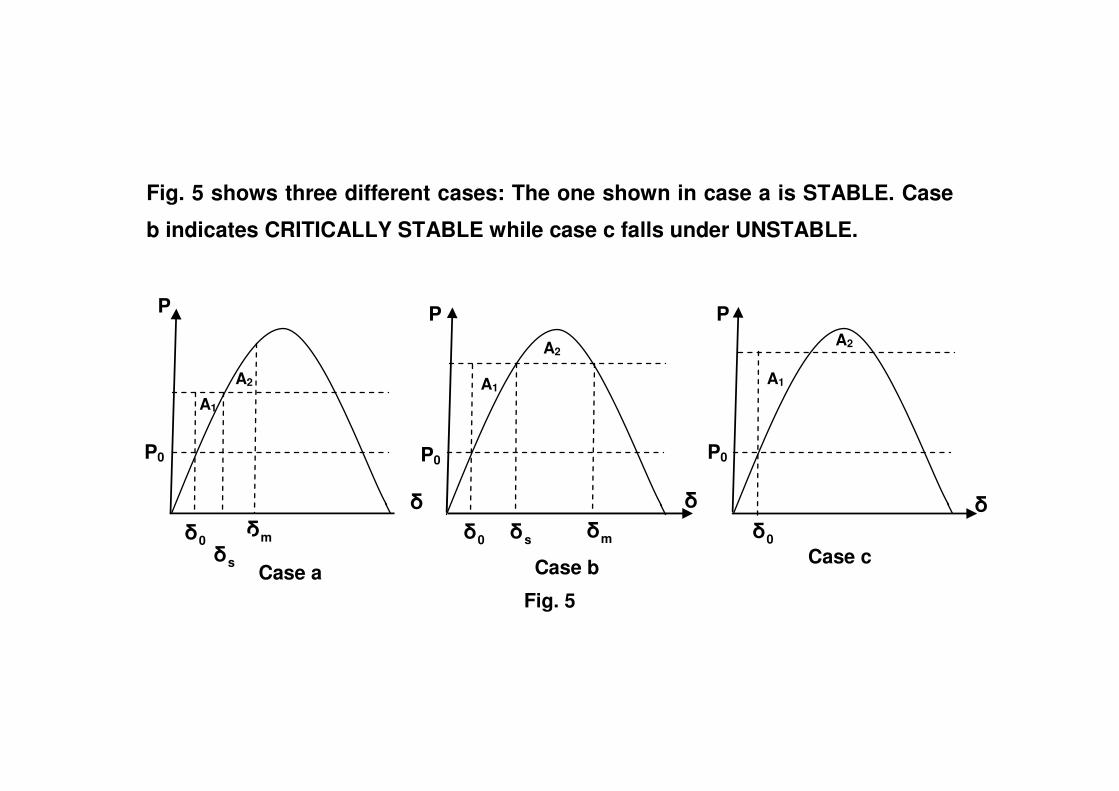
Fig. 5 shows three different cases: The one shown in case a is STABLE. Case

b indicates CRITICALLY STABLE while case c falls under UNSTABLE.

P P

A2

A1

A

A2

P

A2

A1

� �

A1

P0 P0

m�

s� 0�0�

Case c Case b Case a Fig. 5

�

P0

m� s�

0�

Example 1

A synchronous motor having a steady state stability limit of 200 MW is

receiving 50 MW from the infinite bus bars. Find the maximum additional load

that can be applied without causing instability.

Solution

Refereeing to Fig. 6,

for critical stability D C

200

P

A2 PS

�0 = sin-1 .rad0.2526820050 = Further 200 sin �S = PS

for critical stability

A2 = A1

E

D C

B

A

50

�

A1 PS

S�-� s�

0�

Fig. 6

Electric Input power

200 sin �S (� – �S – �0) = �− S

0

��

�

d��sin200 i.e.

(� – �S – �0) sin �S = cos �0 – cos (� – �S) = cos �0 + cos �S i.e.

Adding area ABCDEA to both A1 and A2 and equating the resulting areas

E

D C

B

A

200

50

�

P

A2

A1 PS

S�-� s�

0�

Electric Input power

(� – �S – �0) sin �S = cos �0 – cos (� – �S) = cos �0 + cos �S i.e.

(� – �S – 0.25268) sin �S - cos �S = 0.9682458

The above equation can be solved by trial and error method.

�S 0.85 0.9 0.95

RHS 0.8718 0.9363 0.9954

Using linear interpolation between second and third points we get

�S = 0.927 rad. 0.927 rad. = 53.11 deg.

Thus PS = 200 sin 53.110 = 159.96 MW

Maximum additional load possible = 159.96 – 50 = 109.96 MW

FURTHER APPLICATION OF EQUAL AREA CRITERION

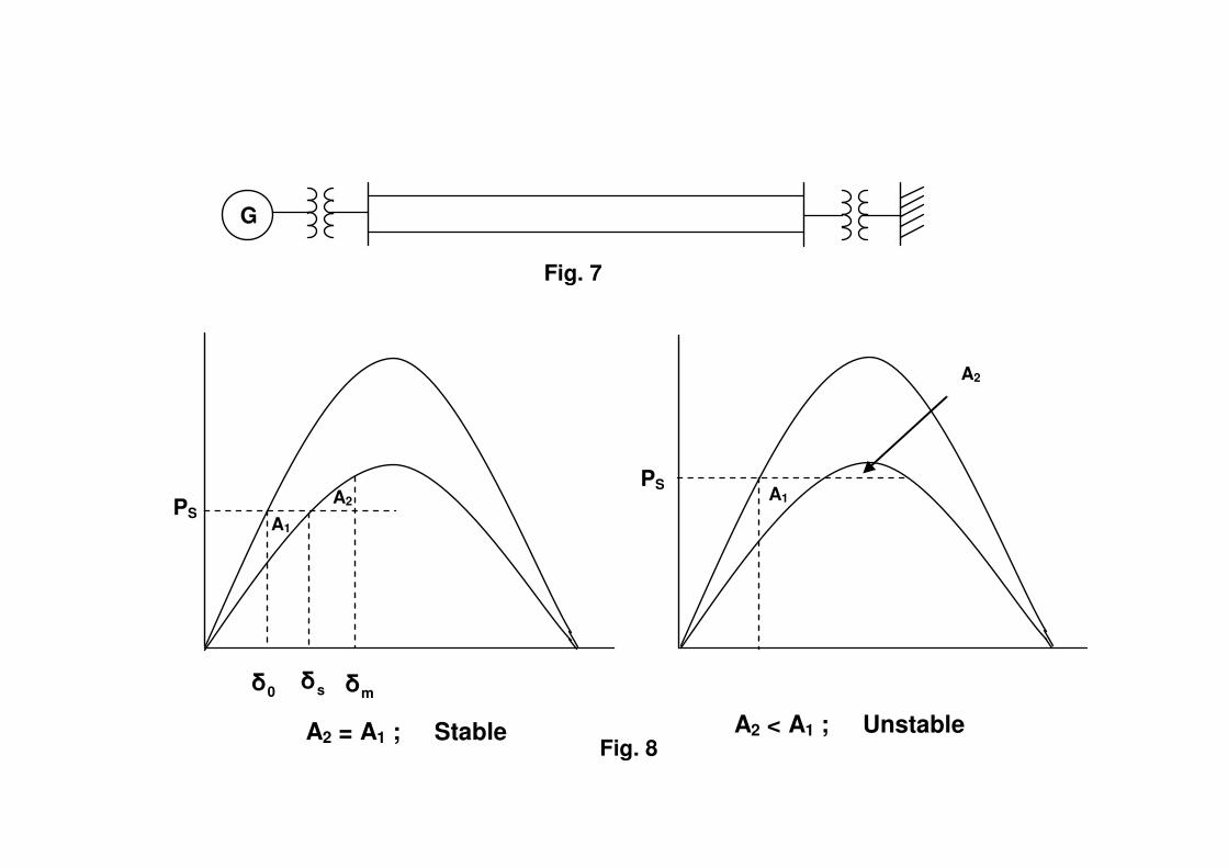
Opening of one of the parallel lines

When a generator is supplying power to an infinite bus over two parallel

transmission lines, the opening of one of the lines will result in increase in the

equivalent reactance and hence decrease in the maximum power transferred.

Because of this, depending upon the initial operating power, the generator

may loose synchronism even though the load could be supplied over the

remaining line under steady state condition. remaining line under steady state condition.

Consider the system shown in Fig. 7. The power angle diagrams

corresponding to stable and unstable conditions are shown in Fig. 8.

G

Fig. 7

G

Fig. 7

A2

Fig. 8

A2 = A1 ; Stable A2 < A1 ; Unstable 0� s�

m�

PS A2

A1

PS A1

Short circuit occurring in the system

Short circuit occurring in the system often causes loss of stability even

though the fault may be removed by isolating it from the rest of the system in a

relatively short time. A three phase fault at one end of a double circuit line is

shown in Fig. 9(a) which can be reduced as shown in Fig. 9(b).

+ Ei

+ Eg

+ Ei

+

It is to be noted that all the current from the generator flows through the fault

and this current Ig lags the generator voltage by 900. Thus the real power

output of the generator is zero. Normally the input power to the generator

remains unaltered. Therefore, if the fault is sustained, the load angle � will

increase indefinitely because all the input power will be used for acceleration,

resulting unstable condition.

Fig. 9

Ig Eg

+

-

Ei -

Eg -

Ei -

(a) (b)

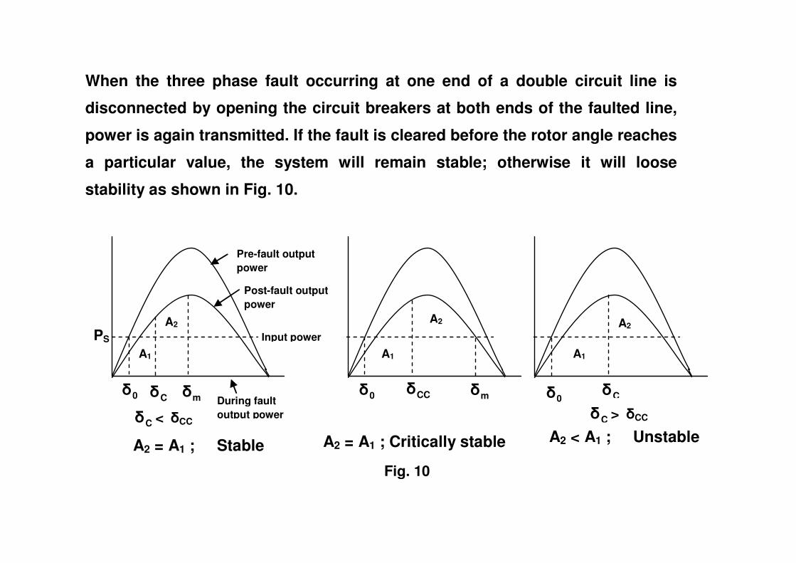
When the three phase fault occurring at one end of a double circuit line is

disconnected by opening the circuit breakers at both ends of the faulted line,

power is again transmitted. If the fault is cleared before the rotor angle reaches

a particular value, the system will remain stable; otherwise it will loose

stability as shown in Fig. 10.

Pre-fault output power

C� C�

Input power

Post-fault output power

C� >���CC C� <���CC

m� 0�

PS

A2

A1

A2 = A1 ; Stable A2 < A1 ; Unstable A2 = A1 ; Critically stable

Fig. 10

During fault output power

0�

A2

A1

CC� m� 0�

A2

A1

When a three phase fault occurs at some point on a double circuit line, other

than on the extreme ends, as shown in Fig. 11(a), there is some finite

impedance between the paralleling buses and the fault. Therefore, some power

is transmitted during the fault and it may be calculated after reducing the

network to a delta connected circuit between the internal voltage of the

generator and the infinite bus as shown in Fig. 11(b).

Xb

Xc Xa Eg

+

-

Em

+

-

(b)

Em

Fig. 11

Eg

+

-

(a)

+

-

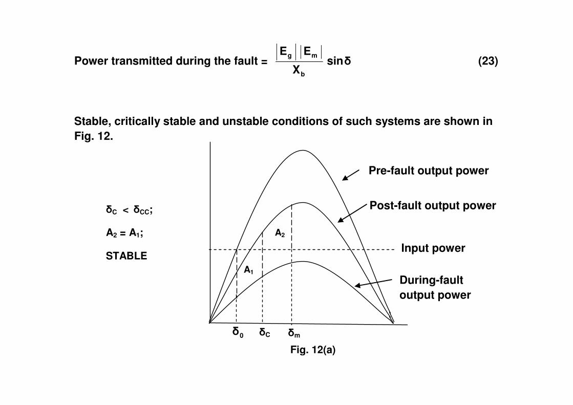
Power transmitted during the fault = �sinX

EE

b

mg (23)

Stable, critically stable and unstable conditions of such systems are shown in Fig. 12.

Post-fault output power

Pre-fault output power

�C <���CC;

A2 = A1;

STABLE

�m �C 0�

A2

A1

Input power

Post-fault output power

During-fault output power

Fig. 12(a)

�C =���CC;

A2 = A1;

CRITICALLYSTABLE

�m �CC 0�

During-fault output power

Input power

Post-fault output power

Pre-fault output power

A1

A2

Fig. 12(b)

�

�

�

�

�

��C 0�

A2

A1 During-fault output power

Input power

Post-fault output power

Pre-fault output power

�C >���CC;

A2 < A1;

UNSTABLE

Fig. 12(c)

m �CC 0�

Example 2

In the power system shown in Fig. 13, three phase fault occurs at P and the

faulty line was opened a little later. Find the power output equations for the

pre-fault, during fault and post-fault conditions.

Values marked are p.u. reactances

P x 1.25E '

g = p.u.

G

Xg’ = 0.28

0.16

0.16 0.16

0.16 0.16

p.u. 1.0V =

Fig. 13

0.24

0.24

Values marked are p.u. reactances

Solution Pre-fault condition

Power output Pe = �sin1.736�sin0.72

1.0x1.25 =

0.56

0.56

0.28

1.25 -

+ -

1.0 +

0.16 0.72

1.0 1.25 +

- -

+

During fault condition:

0.16 0.56

0.28

1.25 - 1.0

+

0.16

0.4

-

+

0.16

0.4 0.16 0.28

0.56

-

+

-

+

Power output Pe = �sin0.418�sin2.99

1.0x1.25 =

1.0 1.25 0.057

0.2 0.08 0.16 0.28

-

+

-

+ 1.25 1.0

2.99

Post-fault condition:

1.0x1.25

1.25 1.0

1.0

0.56

0.28

1.25 - 1.0

+

0.16

-

+

Power output Pe = �sin1.25�sin1.0

1.0x1.25 =

Thus power output equations are:

Pre-fault Pe = Pm1 sin� = 1.736 sin�

During fault Pe = Pm2 sin� = 0.418 sin�

Post fault Pe = Pm3 sin� = 1.25 sin�

Here

Pm1 = 1.736; Pm2 = 0.418; Pm3 = 1.25;

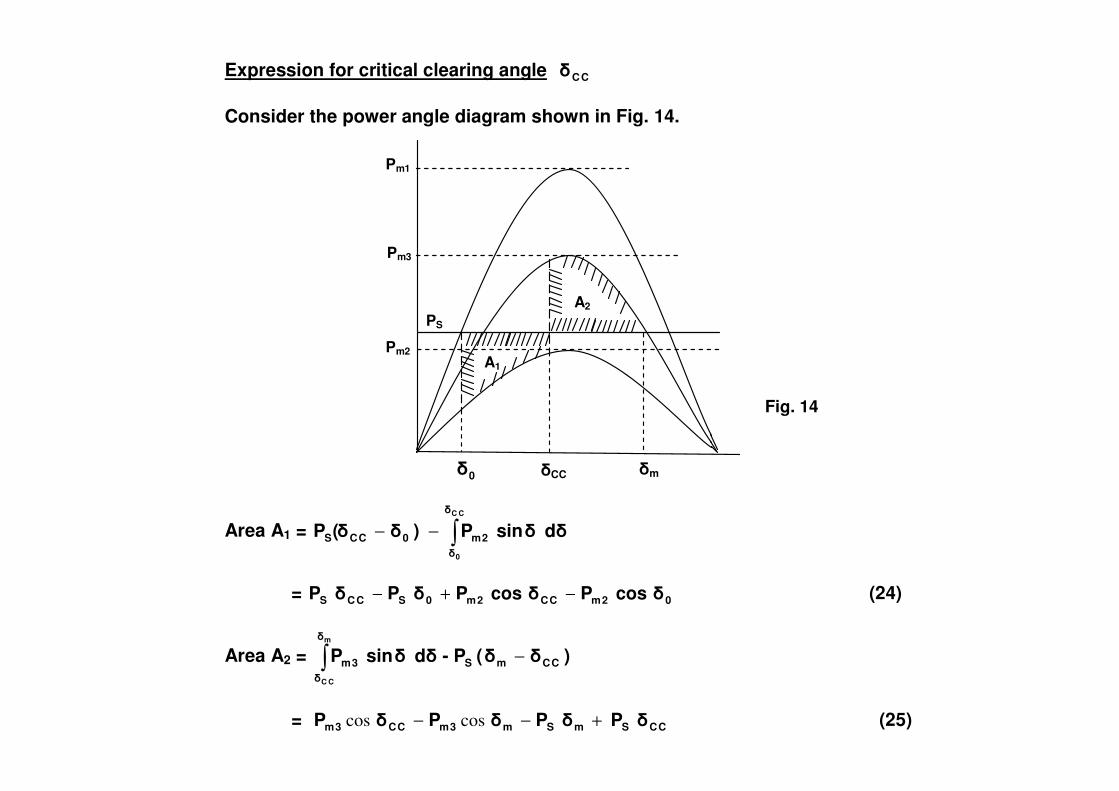
Expression for critical clearing angle CC�

Consider the power angle diagram shown in Fig. 14.

PS

Pm3

A1

A2

Pm2

Pm1

Area A1 = d��sinP)��(PCC

0

�

�

2m0CCS �−−

= 02mCC2m0SCCS �cosP�cosP�P�P −+− (24)

Area A2 = )��(P-d��sinP CCmS

�

�

3m

m

CC

−�

= CCSmSm3mCC3m �P�P�P�P +−− coscos (25)

�m �CC 0�

Fig. 14

Area A1 = 02mCC2m0SCCS �cosP�cosP�P�P −+− (24)

Area A2 = CCSmSm3mCC3m �P�P�P�P +−− coscos (25)

Area A2 = Area A1

CCSmSm3mCC3m �P�P�P�P +−− coscos = 02mCC2m0SCCS �cosP�cosP�P�P −+−

02mm3m0mSCC2m3m �cosP�cosP)��(P�cos)PP( −+−=− 02mm3m0mSCC2m3m �cosP�cosP)��(P�cos)PP( −+−=−

2m3m

02mm3m0mSCC PP

�cosP�cosP)��(P�cos

−−+−

=

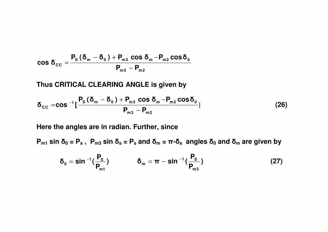
Thus CRITICAL CLEARING ANGLE is given by

]2m3m

02mm3m0mS1CC PP

�cosP�cosP)��(P[cos�

−−+−

= − (26)

2m3m

02mm3m0mSCC PP

�cosP�cosP)��(P�cos

−−+−

=

Thus CRITICAL CLEARING ANGLE is given by

]2m3m

02mm3m0mS1CC PP

�cosP�cosP)��(P[cos�

−−+−

= − (26)

Here the angles are in radian. Further, since

Pm1 sin �0 = Ps , Pm3 sin �s = Ps and �m = �-�s angles �0 and �m are given by

)

PP

(sin�

1m

S10

−=

)PP

(sin��

3m

S1m

−−= (27)

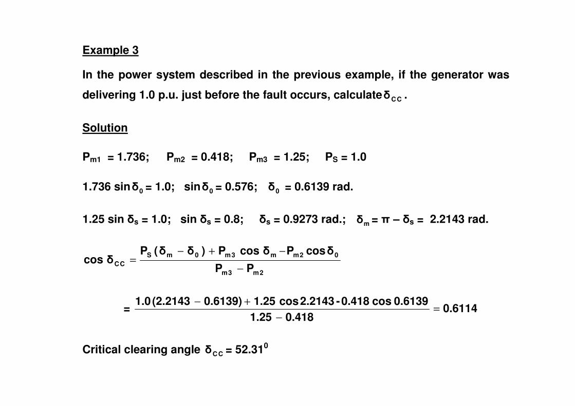
Example 3

In the power system described in the previous example, if the generator was

delivering 1.0 p.u. just before the fault occurs, calculate CC� .

Solution

Pm1 = 1.736; Pm2 = 0.418; Pm3 = 1.25; PS = 1.0

1.736 sin 0� = 1.0; sin 0� = 0.576; 0� = 0.6139 rad.

1.25 sin �s = 1.0; sin �s = 0.8; �s = 0.9273 rad.; m� = � – �s = 2.2143 rad.

2m3m

02mm3m0mSCC PP

�cosP�cosP)��(P�cos

−−+−

=

= 0.61140.4181.25

0.6139 cos 0.418-2.2143cos1.250.6139)(2.21431.0 =−

+−

Critical clearing angle CC� = 52.310

STEP BY STEP SOLUTION OF OBTAINING SWING CURVE

The equal area criterion of stability is useful in determining whether or not a

system will remain stable and in determining the angle through which the

machine may be permitted to swing before a fault is cleared. It does not

determine directly the length of time permitted before clearing a fault if

stability is to be maintained.

In order to specify a circuit breaker of proper speed, the engineer must know

the CRITICAL CLEARING TIME, which is the time for a machine to swing from

its original position to its critical clearing angle. If the Critical Clearing Angle its original position to its critical clearing angle. If the Critical Clearing Angle

(CCA) is determined by the equal area criterion, then to determine

corresponding Critical Clearing Time (CCT), the swing curve for the sustained

faulted condition is required.

The step by step method of obtaining swing curve, using hand calculation is

necessarily simpler than some of the methods recommended for digital

computer. In the method for hand calculation, the change in the angular

position of the rotor during a short interval of time is computed by making the

following assumptions.

1. The accelerating power Pa computed at the beginning of an interval is

constant from the middle of the proceeding interval to the middle of the

interval considered.

2. dtd� is constant throughout any interval at the value computed for the

middle of the interval.

Fig. 15 will help in visualizing the assumptions. The accelerating power is

computed for the points enclosed in circles, at the beginning of n-1, n and n+1

th intervals. The step of P in the figure results from assumption 1. th intervals. The step of Pa in the figure results from assumption 1.

Similarly �’ (dtd� =

dtd� - �s), the excess of angular velocity over the

synchronous angular velocity is shown as a step curve that is constant

throughout the interval, at the value computed at the midpoint.

Between the ordinates n - 23 and n -

21 , there is a change in angular speed �’

caused by constant angular acceleration. This change in angular speed �’ is

t

�t �t

Pa (n)

Pa (n – 1)

Pa

Pa (n – 2)

n n - 1 n - 2 n th interval

n - 1 th interval

�’(n – 1/2) �

’

�’(n – 3/2)

��n

��n-1

t

� n

� n - 2

n - 2 n - 1 n

� n - 1

� t n – 1/2 n – 3/2

Fig. 15

�t �t

� (n – 3/2)

The change in angular speed �’ is

�’(n -

21 ) - �’(n -

23 ) = Constant angular acceleration x time duration

= �tM

P )1n(a − ( Because 2

2

dt�d

= M1 Pa ) (28)

Similarly, change in � over any interval = constant angular speed �’ x time

duration. Thus

1�� (n) = �’(n -

21 ) �t (29)

�� (n – 1) = �’(n - 23 ) �t and (30)

Therefore �� (n) - �� (n – 1) = [ �’(n - 21 ) - �’(n -

23 ) ] �t =

M

P )1n(a − (�t)2

Thus �� (n) = �� (n – 1) + M

P )1n(a − (�t)2 (31)

Thus �� (n) = �� (n – 1) + M

P )1n(a − (�t)2 (31)

Equation (31) shows that the change in torque angle during a given interval is

equal to the change in torque angle during the proceeding interval plus the

accelerating power at the beginning of the interval time Mt)(� 2

.

Torque angle � can be computed as

� (n) = � (n – 1) + �� (n) (32)

where �� (n) = �� (n – 1) + M

P )1n(a − (�t)2 (33)

The process of computation is now repeated to obtain Pa (n), �� (n+1) and � (n+1).

The solution in discrete form is thus carried out over the desired length of time

normally 0.05 sec. Greater accuracy of solution can be achieved by reducing

the time duration of interval.

Any switching event such as occurrence of a fault or clearing of the fault

causes discontinuity in the accelerating power Pa. If such a discontinuity

occurs at the beginning of an interval then the average of the values of Pa just

before and just after the discontinuity must be used.

Thus in computing the increment of angle occurring during the first interval

after a fault is applied at time t = 0 becomes

��1 = 0 + 21 (Pa 0

- + Pa 0+)

Mt)(� 2

= 21 Pa 0

+ Mt)(� 2

(Because Pa 0- = 0)

If the discontinuity occurs at the middle of an interval, no special procedure is

needed. The correctness of this can be seen from Fig. 16.

n th interval

n - 1 th interval

n th interval

n - 1 th interval

Discontinuity at the beginning of an interval

Discontinuity at the middle of an interval

Fig. 16

Example 4

A 20 MVA, 50 Hz generator delivers 18 MW over a double circuit line to an

infinite bus. The generator has KE of 2.52 MJ / MVA at rated speed and its

transient reactance is Xd’ = 0.35 p.u. Each transmission line has a reactance of

0.2 p.u. on a 20 MVA base. E = 1.1 p.u. and infinite bus voltage V = 1.0 p.u. A

three phase fault occurs at the mid point of one of the transmission lines.

Obtain the swing curve over a period of 0.5 sec. if the fault is sustained.

E = 1.1 p.u. 0.2 p.u.

��

G = 20 MVA = 1.0 p.u.

Angular momentum M = deg.elec./sec10x2.850x180

2.52x1.0f180

HG 24−==

Let us choose �t = 0.05 sec. Mt)(� 2

= 8.9292.8

10x(0.05) 42

=

20 MVA 50 Hz Delivers 18 MW Xd

’ = 0.35 p.u. H = 2.52 MJ/MVA

Infinite bus

V = 1.0 p.u.

0.2 p.u. ��

Recursive equations are � (n) = � (n – 1) + �� (n)

where �� (n) = �� (n – 1) + 8.929 Pa (n-1)

Pre fault: X = 0.45 p.u.; Pe = � sin 2.44�sin0.45

1.0x1.1 =

During fault:

0.1 0.2

0.35

1.1 - 1.0

+

0.1

+ 0.1 0.1 0.35

0.2

+ +

Converting the star 0.35, 0.1 and 0.2 as delta

Pe = � sin 0.88�sin1.25

1.0x1.1 =

1.1 - - - -

1.1 1.0

1.25

Initial calculations:

Before the occurrence of fault, there will not be acceleration i.e. Input power is

equal to output power. Therefore

Ps = 18 MW = 0.9 p.u.

Initial power angle is given by

2.44 0� sin = 0.9; Thus 0� = 21.64

Pa 0- = 0; Pa 0

+ = 0.9 – 0.88 sin 21.640 = 0.576 p.u.

Pa average = ( 0 + 0.576 ) / 2 = 0.288 p.u.

First interval: ��1 = 0 + Pa average x Mt)(� 2

= 0.288 x 8.929 = 2.570

Thus �(0.05) = 21.64 + 2.57 = 24.210

Subsequent calculations are shown below.

t sec. � deg. Pmax Pe Pa = 0.9-Pe 8.929 Pa ��

0- 21.64 0

0+ 21.64 0.88 0.324 0.576

0 average 21.64 0.288 2.57 2.57

0.05 24.21 0.88 0.361 0.539 4.81 7.38

0.10 31.59 0.88 0.461 0.439 3.92 11.30

0.15 42.89 0.88 0.598 0.301 2.68 13.98

0.20 56.87 0.88 0.736 0.163 1.45 15.43

0.25 72.30 0.88 0.838 0.062 0.55 15.98

0.30 88.28 0.88 0.879 0.021 0.18 16.16

0.35 104.44 0.88 0.852 0.048 0.426 16.58

0.40 121.02 0.88 0.754 0.145 1.30 17.88

0.45 138.90 0.88 0.578 0.321 2.87 20.75

0.50 159.65

�

����

���

����

����

����

����

�

�

�

�

�

�

���� ���

���

��

���

����

���

��� ���� ��� ���� ��� ���� ���

�

�

�

�

�

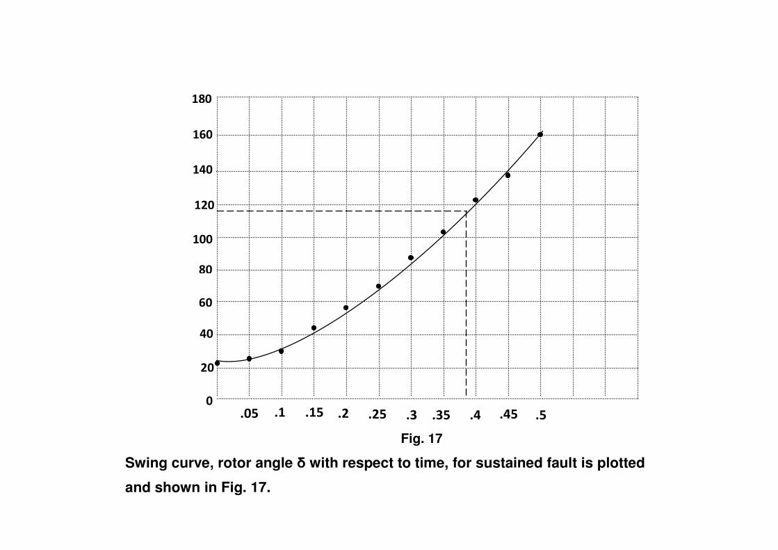
Swing curve, rotor angle � with respect to time, for sustained fault is plotted

and shown in Fig. 17.

Fig. 17

Example 5

In the power system considered in the previous example, fault is cleared by

opening the circuit breakers at both ends of the faulty line. Calculate the CCA

and hence find CCT.

Solution

From the previous example: Ps = 0.9; Pm1 = 2.44 and Pm2 = 0.88

For the Post fault condition:

X = 0.55 p.u; Pe = � sin 2.0�sin0.55

1.0x1.1 =

Thus Ps = 0.9; Pm1 = 2.44; Pm2 = 0.88; Pm3 = 2.0

2m3m

02mm3m0mSCC PP

�cosP�cosP)��(P�cos

−−+−

= �

2.44 sin �0 = 0.9; Therefore �0 = 0.3778 rad.

2.0 sin �s = 0.9; Thus �s = 0.4668 Therefore �m = � - �s = 2.6748 rad

0.479150.882

(0.3778)cos0.88(2.6748)cos2)0.37782.6748(0.9�cos CC −=

−−+−=

Thus CCA, �CC = 118.630

����

���

���

����

����

����

����

���� ���

���

��

���

����

���

��� ���� ��� ���� ��� ���� ���

Referring to the swing curve obtained for the sustained fault condition,

corresponding to CCA of 118.630, CCT can be obtained as 0.38 sec. as shown

in Fig. 18.

Fig. 18

ADDITIONAL EXAMPLES

Following Examples 6,7 and 8 will help in understanding the digital computer

solution for multi-machine stability.

Example 6

The single-line diagram of Fig. 19 shows a 50 Hz. generator connected through

parallel transmission lines to a large metropolitan system considered as an

infinite bus. The machine is delivering 1.0 per unit power and both the terminal

voltage and infinite bus voltages are 1.0 per unit. The numbers marked on the

diagram indicate the values of the reactances on a common system base. The

transient reactance of the generator is 0.2 per unit. (i) Calculate the internal

voltage (ii) Determine the power angle equation for the system. (iii) Find the

operating rotor angle. (iv) Obtain the swing equation. Take H = 5 MJ / MVA.

Infinite bus

j 0.1

j 0.4

j 0.4

�

X ‘d = 0.2

Fig. 19

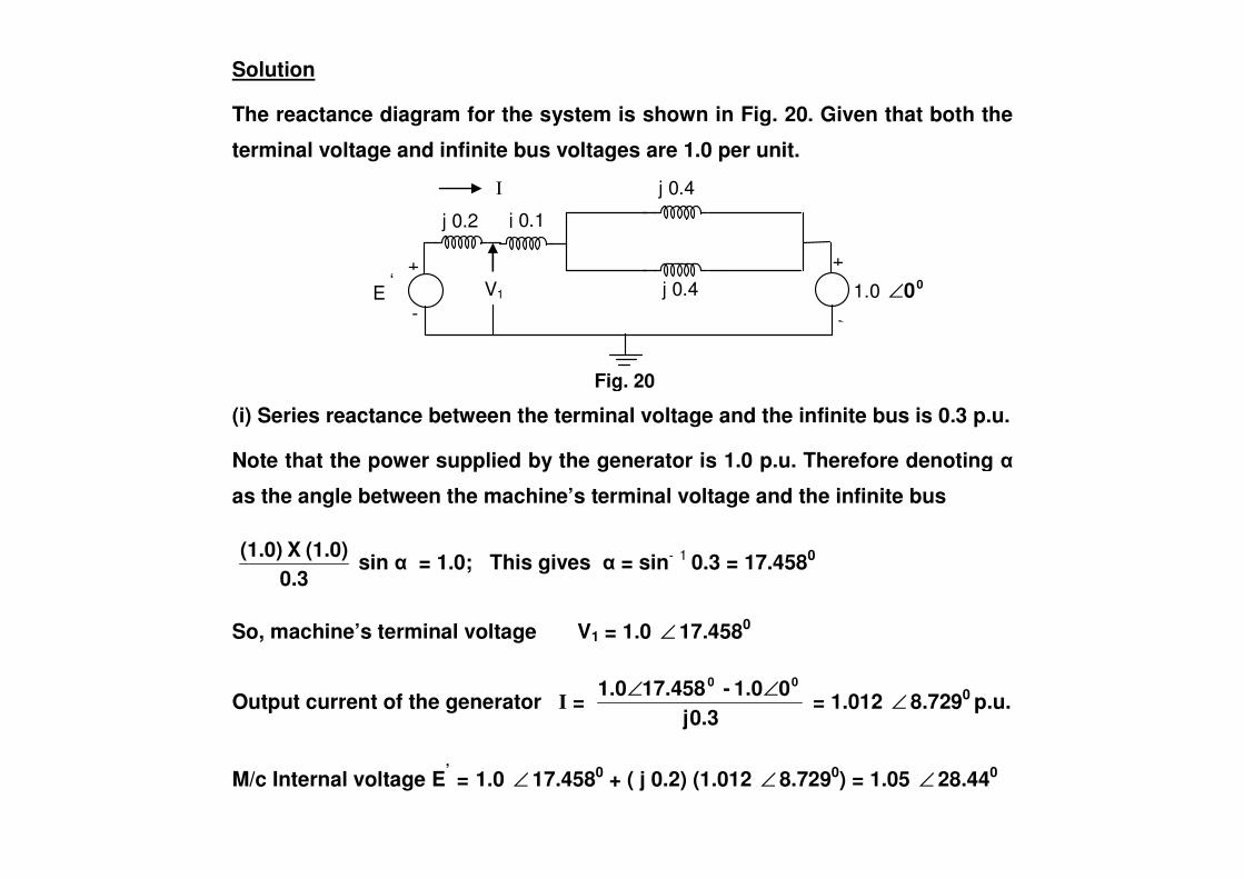
Solution

The reactance diagram for the system is shown in Fig. 20. Given that both the

terminal voltage and infinite bus voltages are 1.0 per unit.

(i) Series reactance between the terminal voltage and the infinite bus is 0.3 p.u.

+

-

1.0 00∠

Fig. 20

j 0.1 j 0.2

j 0.4

j 0.4

+

-

E ‘ �� V1

I

Note that the power supplied by the generator is 1.0 p.u. Therefore denoting �

as the angle between the machine’s terminal voltage and the infinite bus

0.3(1.0) X (1.0) sin � = 1.0; This gives � = sin- 1�0.3 = 17.4580

So, machine’s terminal voltage V1 = 1.0 ∠ 17.4580

Output current of the generator I = 0.3j

01.0 -17.4581.0 00 ∠∠ = 1.012 ∠ 8.7290 p.u.

M/c Internal voltage E’ = 1.0 ∠ 17.4580 + ( j 0.2) (1.012 ∠ 8.7290) = 1.05 ∠ 28.440

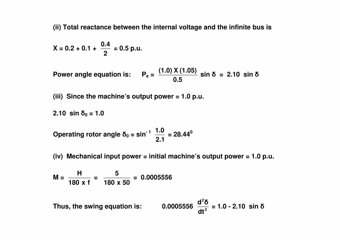
(ii) Total reactance between the internal voltage and the infinite bus is

X = 0.2 + 0.1 + 2

0.4 = 0.5 p.u.

Power angle equation is: Pe = 0.5

(1.05) X (1.0) sin � = 2.10 sin �

(iii) Since the machine’s output power = 1.0 p.u.

2.10 sin �0 = 1.0

Operating rotor angle �0 = sin- 1 2.11.0 = 28.440

(iv) Mechanical input power = initial machine’s output power = 1.0 p.u.

M = fx180

H = 50x180

5 = 0.0005556

Thus, the swing equation is: 0.0005556 2

2

dt�d

= 1.0 - 2.10 sin �

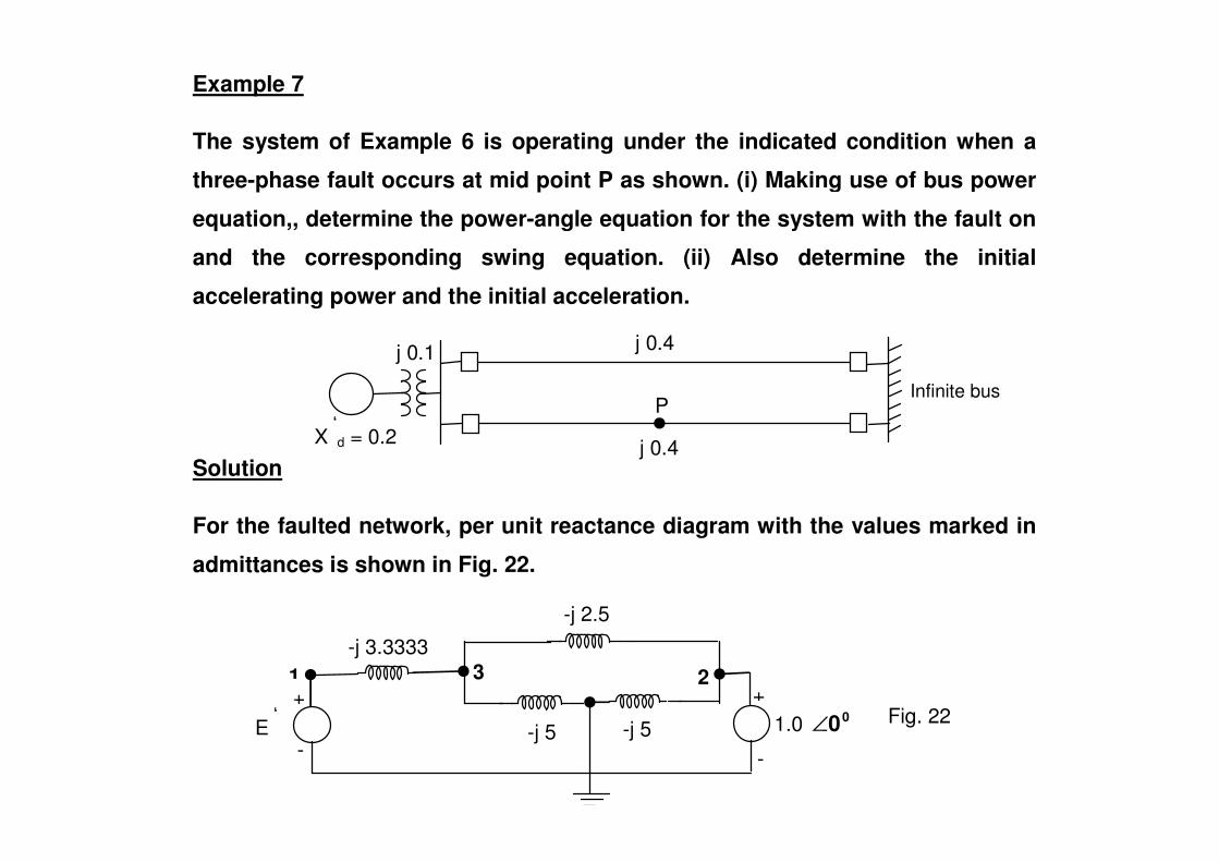
Example 7

The system of Example 6 is operating under the indicated condition when a

three-phase fault occurs at mid point P as shown. (i) Making use of bus power

equation,, determine the power-angle equation for the system with the fault on

and the corresponding swing equation. (ii) Also determine the initial

accelerating power and the initial acceleration.

X ‘ = 0.2

P Infinite bus

j 0.1 j 0.4

�

Solution

For the faulted network, per unit reactance diagram with the values marked in

admittances is shown in Fig. 22.

+

-

1.0 00∠

1 2 3 -j 3.3333

-j 5

-j 2.5

+

-

E ‘ �� -j 5

X ‘d = 0.2 j 0.4

Fig. 22

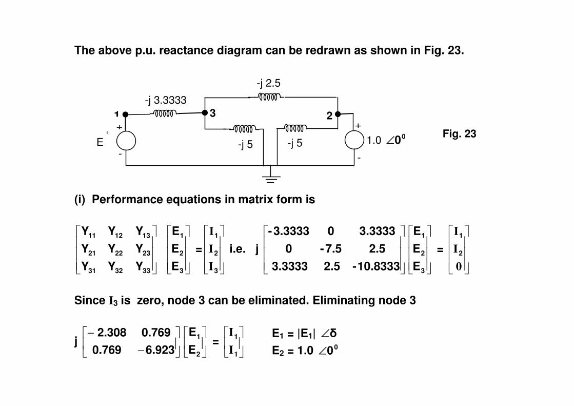
The above p.u. reactance diagram can be redrawn as shown in Fig. 23.

(i) Performance equations in matrix form is

Fig. 23 +

-

1.0 00∠

1 2 3 -j 3.3333

-j 5

-j 2.5

+

-

E ‘ �� -j 5

E1 = |E1| �∠E2 = 1.0 00∠

(i) Performance equations in matrix form is

���

�

�

���

�

�

333231

232221

131211

YYYYYYYYY

���

�

�

���

�

�

3

2

1

EEE

=���

�

�

���

�

�

3

2

1

III

i.e. j ���

�

�

���

�

�

10.8333-2.53.33332.57.5-0

3.333303.3333-

���

�

�

���

�

�

3

2

1

EEE

= ���

�

�

���

�

�

0II

2

1

Since I3 is zero, node 3 can be eliminated. Eliminating node 3

j ��

���

�

−−

6.9230.7690.7692.308

��

���

�

2

1

EE

= ��

���

�

1

1

II

As discussed in power flow analysis, real power injection at bus i is

Pi = )��(cosYVV inninin

N

1ni −+�

=

ϑ

In this case, power flow from node 1 to 2 is

P1 = |E1| |E2| |Y12| cos (90 + 0 – �)

= |E1| |E2| |Y12| sin �

Thus during fault generator power output Pe = 1.05 x 1.0 x 0.768 sin �

= 0.808 sin �

Corresponding swing equation is: 0.0005556 2

2

dt�d = 1.0 – 0.808 sin �

(ii) Rotor angle � is initially 28.440 as in Example 6.

Therefore initial accelerating power = Ps - Pe = 1.0 - 0.808 sin 28.44 = 0.615 p.u.

Initial acceleration 2

2

dt�d

= 0.0005556

0.615

= 1107 elec. deg. / sec.2

Example 8

The fault on the system of Example 7 is cleared by simultaneous opening of

the circuit breakers at each end of the affected line. Determine the power-angle

equation and the swing equation for the post-fault period.

Solution

Corresponding reactance diagram can be obtained as shown in Fig. 24.

Fig. 24 +

-

1.0 00∠

1 2 3 -j 3.3333

-j 2.5

+

-

E ‘ ��

( j 0.4 )

( j 0.3 )

Admittance y12 =0.7 j1

= - j 1.429 p.u.

Therefore, the transfer admittance Y = - y = j 1.429

Fig. 24 +

-

1.0 00∠

1 2 3 -j 3.3333

-j 2.5

+

-

E ‘ ��

( j 0.4 )

( j 0.3 )

Therefore, the transfer admittance Y12 = - y12 = j 1.429

Therefore post fault power-angle equation is

Pe = 1.05 x 1.0 x 1.429 sin �

= 1.5 sin �

and the corresponding swing equation is

0.0005556 2

2

dt�d

= 1.0 – 1.5 sin �

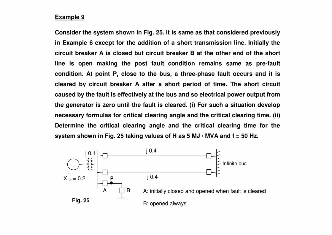
Example 9

Consider the system shown in Fig. 25. It is same as that considered previously

in Example 6 except for the addition of a short transmission line. Initially the

circuit breaker A is closed but circuit breaker B at the other end of the short

line is open making the post fault condition remains same as pre-fault

condition. At point P, close to the bus, a three-phase fault occurs and it is

cleared by circuit breaker A after a short period of time. The short circuit

caused by the fault is effectively at the bus and so electrical power output from

the generator is zero until the fault is cleared. (i) For such a situation develop

necessary formulas for critical clearing angle and the critical clearing time. (ii) necessary formulas for critical clearing angle and the critical clearing time. (ii)

Determine the critical clearing angle and the critical clearing time for the

system shown in Fig. 25 taking values of H as 5 MJ / MVA and f = 50 Hz.

P

Fig. 25

A: initially closed and opened when fault is cleared

B: opened always

B A

Infinite bus

j 0.1

j 0.4

j 0.4

�

X ‘d = 0.2

Solution

For the system described the power-angle curve showing the critical clearing

angle �cc is shown in Fig. 26.

Swing equation for during fault is

M 2

2

dt�d

= Ps – 0 i.e. 2

2

dt�d

= M1 Ps

Integrating the above once

dtd� =

M1 Ps t (

dtd� at t = 0 is zero)

Pm

Fig. 26

Ps

�m �cc �0 0

A1

A2

A further integration with respect time yields the rotor angle as

�(t) = M21 Ps t2 + �0

Corresponding to critical clearing angle �cc, critical clearing time is tccT. Thus

�cc = M21 Ps tccT

2 + �0; i.e. tccT2 =

sPM2 ( �cc – �0 ) Thus

Critical clearing time tccT = )0ccs

�(�P

M2 −

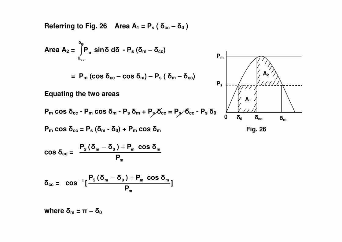
Referring to Fig. 26 Area A1 = Ps ( �cc – �0 )

Area A2 = �m

cc

�

�

m d��sinP - Ps (�m – �cc)

= Pm (cos �cc – cos �m) – Ps ( �m – �cc)

Equating the two areas

Pm cos �cc - Pm cos �m - Ps �m + Ps �cc = Ps �cc - Ps �0

Pm

Ps

�m �cc �0 0

A1

A2

Pm cos �cc = Ps (�m - �0) + Pm cos �m

cos �cc = m

mm0mS

P

�cosP)��(P +−

�cc = ]P

�cosP)��(P[cos

m

mm0mS1 +−−

where �m = � – �0

Fig. 26

�m

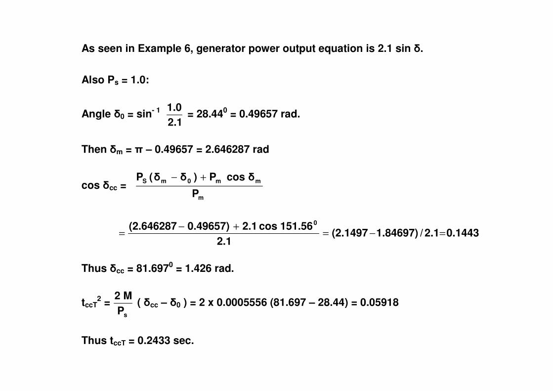
As seen in Example 6, generator power output equation is 2.1 sin �.

Also Ps = 1.0:

Angle �0 = sin- 1 2.11.0 = 28.440 = 0.49657 rad.

Then �m = � – 0.49657 = 2.646287 rad

cos �cc = m

mm0mS

P

�cosP)��(P +−

mP

0.14432.1/1.84697)(2.14972.1

151.56cos2.10.49657)(2.646287 0

=−=+−=

Thus �cc = 81.6970 = 1.426 rad.

tccT2 =

sPM2 ( �cc – �0 ) = 2 x 0.0005556 (81.697 – 28.44) = 0.05918

Thus tccT = 0.2433 sec.

SOLUTION OF SWING EQUATION BY MODIFIED EULER’S METHOD

Modified Euler’s method is simple and efficient method of solving differential

equations (DE)

Let us first consider solution of first order differential equation. Later we shall

extend it for solving a set of first order DE. The swing equation is a second

order DE which can be written as two first order DE and solution can be

obtained using Modified Euler’s method.

Let the given first order DE be

)xt,(fdtdx = (34)

where t is the independent variable and x is the dependent variable. Let (t 0, x 0)

be the initial solution and �t is the increment in t. Then

t 1 = t 0 + �t; t 2 = t 1 + �t; t n = t n – 1 + �t

First estimate of x1 is denoted as x 1(0). Then

x 1(0) = x 0 +

dtdx |0 �t (35)

Thus (t 1, x 1(0)) is the first estimated point of (t 1, x 1). Second and the final

estimate of x 1 is calculated as

x 1 = x 0 + dtdx

(21 |0 +

dtdx |1(0)) �t (36)

where dtdx |1(0)) is the value of

dtdx computed at (t 1, x 1

(0)). Thus the next point

(t 1, x 1) is now known. Same procedure can be followed to get (t 2, x 2) and it

can be repeated to obtain points (t 3, x 3), (t 4, x 4) ……..

Knowing (t n - 1, x n - 1 ), next point (t n, x n) can be computed as follows:

x n(0) = x n – 1 + dtdx |n – 1 �t (37)

t n = t n – 1 + �t (38)

Compute dtdx |n(0) which is

dtdx computed at (t n, x n(0)). (39)

Then x n = x n - 1 + dtdx

(21 |n - 1 +

dtdx |n(0)) �t (40)

Same procedure can be extended to solve a set of two first order DE. Let the

DE be

dtdx = f1 (t, x, y) and

dtdy = f2 (t, x, y)

Knowing (t n - 1, x n - 1 , y n - 1), next point (t n, x n, yn) can be computed as follows:

x n(0) = x n – 1 + dtdx |n – 1 �t

y n(0) = y n – 1 + dtdy |n – 1 �t

t n = t n – 1 + �t

Compute dtdx |n(0) which is

dtdx computed at (t n, x n(0), y n

(0)) and

dtdy |n(0) which is

dtdy computed at (t n, x n(0), y n

(0))

Then x n = x n - 1 + dtdx

(21 |n - 1 +

dtdx |n(0)) �t and

y n = y n - 1 + dtdy

(21 |n - 1 +

dtdy |n(0)) �t

We know that the swing equation is

M 2

2

dt�d = Pa

When per unit values are used and the machine’s rating is taken as base

M = f�

H

Therefore for a generator

2

2

dt�d = )PP(

Hf�

es − = K ( Ps – Pe ) where K = H

f�

The second order DE

2

2

dt�d = K ( Ps – Pe ) can be written as two first order DE’s given by

dtd� = � – �s

dtd� = K ( Ps – Pe )

Note that dtd� generally of the form

dtd� = f1 ( t, �, �). However, now it a

function of � alone. Similarly, dtd� generally of the form

dtd� = f2 ( t, �, �).

However, now it a function of � alone.

Just prior to the occurrence of the disturbance, Ps – Pe = 0 and � = �s. The

rotor angle can be computed as �(0) and the corresponding angular velocity is

�(0). Thus the initial point is ( 0, �(0), �(0)).

As soon as disturbance occurs, electric network changes and the expression

for electric power Pe in terms of rotor angle � can be obtained. During fault

condition, Pe shall be computed by the said expression.

Using Modified Euler’s method �1 and �1 can be computed. Thus we get the

next solution point as ( t1, �1, �1). The procedure can be repeated to get

subsequent solution points until next change in electric network, such as

removal of faulted line occurs. As soon as electric network changes,

corresponding expression for electric power need to be obtained and used in

subsequent calculation.

The whole procedure can be carried out until t reaches the time upto which

transient stability analysis is required.

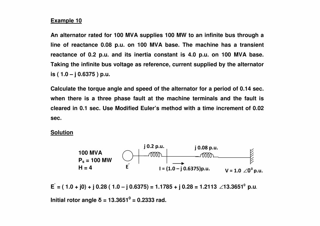
Example 10

An alternator rated for 100 MVA supplies 100 MW to an infinite bus through a

line of reactance 0.08 p.u. on 100 MVA base. The machine has a transient

reactance of 0.2 p.u. and its inertia constant is 4.0 p.u. on 100 MVA base.

Taking the infinite bus voltage as reference, current supplied by the alternator

is ( 1.0 – j 0.6375 ) p.u.

Calculate the torque angle and speed of the alternator for a period of 0.14 sec.

when there is a three phase fault at the machine terminals and the fault is

cleared in 0.1 sec. Use Modified Euler’s method with a time increment of 0.02

100 MVA Ps = 100 MW H = 4

������������

�������� 00∠ �����

�����������

� �

����!������������"�#�����

sec.

Solution

E’ = ( 1.0 + j0) + j 0.28 ( 1.0 – j 0.6375) = 1.1785 + j 0.28 = 1.2113 .p.u13.36510∠

Initial rotor angle � = 13.36510 = 0.2333 rad.

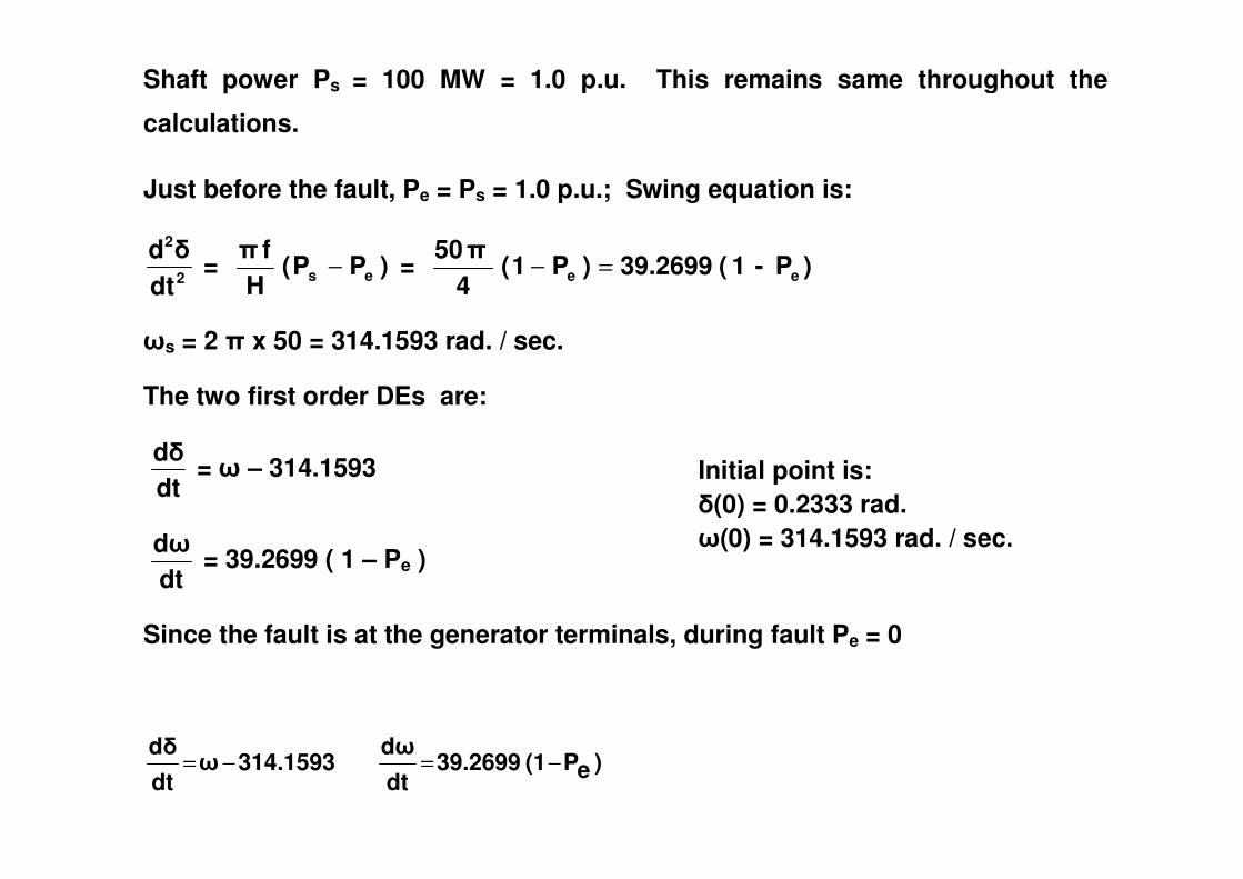
Shaft power Ps = 100 MW = 1.0 p.u. This remains same throughout the

calculations.

Just before the fault, Pe = Ps = 1.0 p.u.; Swing equation is:

2

2

dt�d

= )PP(H

f�es − = )P - 1 ( 39.2699)P1(

4�50

ee =−

�s = 2 � x 50 = 314.1593 rad. / sec.

The two first order DEs are:

d�Initial point is: �(0) = 0.2333 rad. �(0) = 314.1593 rad. / sec.

dtd� = � – 314.1593

dtd� = 39.2699 ( 1 – Pe )

Since the fault is at the generator terminals, during fault Pe = 0

)eP(139.2699dtd�

314.1593�dtd�

−=−=

Initial point is: �(0) = 0.2333 rad. �(0) = 314.1593 rad. / sec.

To calculate �(0.02) and �(0.02)

First estimate:

dtd� = 314.1593 – 314.1593 = 0

dtd� = 39.2699 ( 1 – 0 ) = 39.2699

� = 0.2333 + ( 0 x 0.02 ) = 0.2333 rad.

� = 314.1593 + ( 39.2699 x 0.02 ) = 314.9447 rad. / sec.

Second estimate: First estimated point is: � = 0.2333 rad. � = 314.9447 rad. / sec.

Second estimate:

dtd� = 314.9447 – 314.1593 = 0.7854

dtd� = 39.2699 ( 1 – 0 ) = 39.2699; Thus

�(0.02) = 0.2333 + 21 ( 0 + 0.7854 ) x 0.02 = 0.24115 rad.

�(0.02) = 314.1593 + 21 ( 39.2699 + 39.2699 ) x 0.02 = 314.9447 rad. / sec.

Latest point is: �(0.02) = 0.24115 rad. �(0.02) = 314.9447 rad. / sec.

)eP(139.2699dtd�

314.1593�dtd�

−=−=

To calculate �(0.04) and �(0.04)

First estimate

dtd� = 314.9447 – 314.1593 = 0.7854

dtd� = 39.2699 ( 1 – 0 ) = 39.2699

� = 0.24115 + ( 0.7854 x 0.02 ) = 0.2569 rad.

� = 314.9447 + ( 39.2699 x 0.02 ) = 315.7301 rad. / sec.

First estimated point is: � = 0.2569 rad. � = 315.7301 rad. / sec.

� = 314.9447 + ( 39.2699 x 0.02 ) = 315.7301 rad. / sec.

Second estimate:

dtd� = 315.7301 – 314.1593 = 1.5708

dtd� = 39.2699 ( 1 – 0 ) = 39.2699; Thus

�(0.04) = 0.24115 + 21 ( 0.7854 + 1.5708 ) x 0.02 = 0.2647 rad.

�(0.04) = 314.9447 + 21 ( 39.2699 + 39.2699 ) x 0.02 = 315.7301 rad. / sec.

Calculations can be repeated until the fault is cleared i.e. t = 0.1-. The results

are tabulated. Thus

�(0.1) = 0.4297 rad.; �(0.1) = 318.0869 rad. / sec.

Once the fault is cleared, reactance between internal voltage and the infinite

bus is 0.28 and thus generator out put is;

Pe = �sin4.3261�sin0.28

1.0x1.2113 =

In the subsequent calculation Pe must be obtained from the above equation.

)eP(139.2699dtd�

314.1593�dtd�

−=−=

Latest point is: �(0.1) = 0.4297 rad. �(0.1) = 318.0869 rad. / sec.

To calculate �(0.12) and �(0.12)

First estimate

dtd� = 318.0869 – 314.1593 = 3.9276

dtd� = 39.2699 ( 1 – 4.3261 sin 0.4297 rad. ) = - 31.5041

� = 0.4297 + ( 3.9276 x 0.02 ) = 0.50825 rad.

� = 318.0869 + (- 31.5041 x 0.02 ) = 317.4568 rad. / sec.

Second estimate: First estimated point is: � = 0.50825 rad. � = 317.4568 rad. / sec.

Second estimate:

dtd� = 317.4568 – 314.1593 = 3.2975

dtd� = 39.2699 ( 1 – 4.3261 sin 0.50825 rad. ) = - 43.4047; Thus

�(0.12) = 0.4297 + 21 ( 3.9276 + 3.2975 ) x 0.02 = 0.50195 rad.

�(0.12) = 318.0869 + 21 ( - 31.5041 - 43.4047 ) x 0.02 = 317.3378 rad. / sec�

Complete calculations are shown in the Table:

);eP(139.2699dtd�

314.1593;�dtd�

−=−= ��Pe = 0 for t < 0.1 and then Pe = 4.3261 sin �

t sec.

� rad. � rad/sec

First Estimate Second Estimate

d�/dt d�/dt � rad. �

rad/sec d�/dt d�/dt � rad. �

rad/sec

0- 0.2333 314.1593

0+ 0.2333 314.1593 0 39.2699 0.2333 314.9447 0.7854 39.2699 0.2412 314.9447

0.02 0.2412 314.9447 0.7854 39.2699 0.2569 315.7301 1.5708 39.2699 0.2647 315.7301 0.02 0.2412 314.9447 0.7854 39.2699 0.2569 315.7301 1.5708 39.2699 0.2647 315.7301

0.04 0.2647 315.7301 1.5708 39.2699 0.2961 316.5155 2.3562 39.2699 0.304 316.5155

0.06 0.304 316.5155 2.3562 39.2699 0.3511 317.3009 3.1416 39.2699 0.359 317.3009

0.08 0.359 317.3009 3.1416 39.2699 0.4218 318.0863 3.927 39.2699 0.4297 318.0869

0.10- 0.4297 318.0869

0.10+ 0.4297 318.0869 3.9276 -31.504 0.5083 317.4568 3.2975 -43.405 0.502 317.3378

0.12 0.502 317.3378 3.1785 -42.468 0.5655 316.4884 2.3291 -51.761 0.557 316.3955

0.14 0.557 316.3955

�

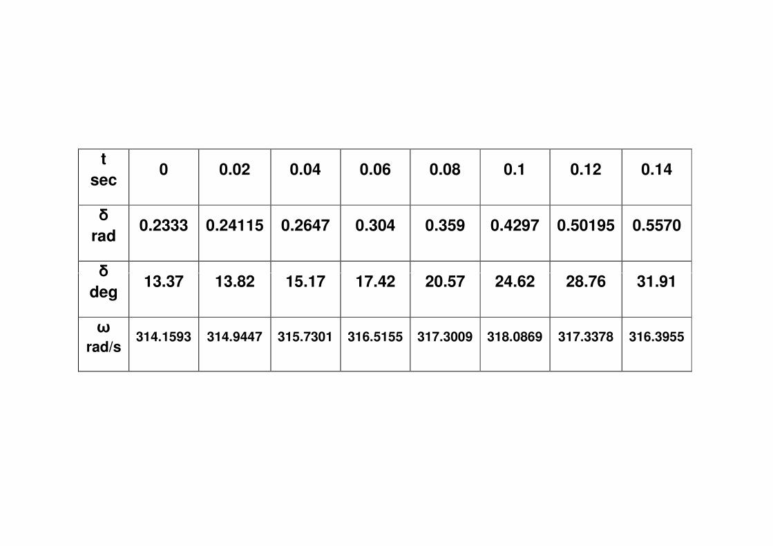
t sec

0 0.02 0.04 0.06 0.08 0.1 0.12 0.14

� rad

0.2333 0.24115 0.2647 0.304 0.359 0.4297 0.50195 0.5570

� 13.37 13.82 15.17 17.42 20.57 24.62 28.76 31.91

� deg

13.37 13.82 15.17 17.42 20.57 24.62 28.76 31.91

� rad/s

314.1593 314.9447 315.7301 316.5155 317.3009 318.0869 317.3378 316.3955

�

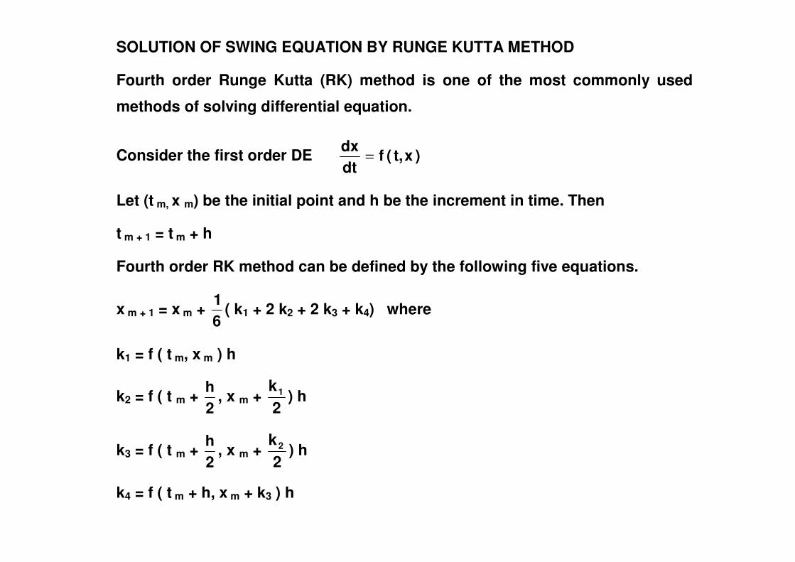
SOLUTION OF SWING EQUATION BY RUNGE KUTTA METHOD

Fourth order Runge Kutta (RK) method is one of the most commonly used

methods of solving differential equation.

Consider the first order DE )xt,(fdtdx =

Let (t m, x m) be the initial point and h be the increment in time. Then

t m + 1 = t m + h

Fourth order RK method can be defined by the following five equations.

x m + 1 = x m + 61 ( k1 + 2 k2 + 2 k3 + k4) where

k1 = f ( t m, x m ) h

k2 = f ( t m + 2h , x m +

2k1 ) h

k3 = f ( t m + 2h , x m +

2k2 ) h

k4 = f ( t m + h, x m + k3 ) h

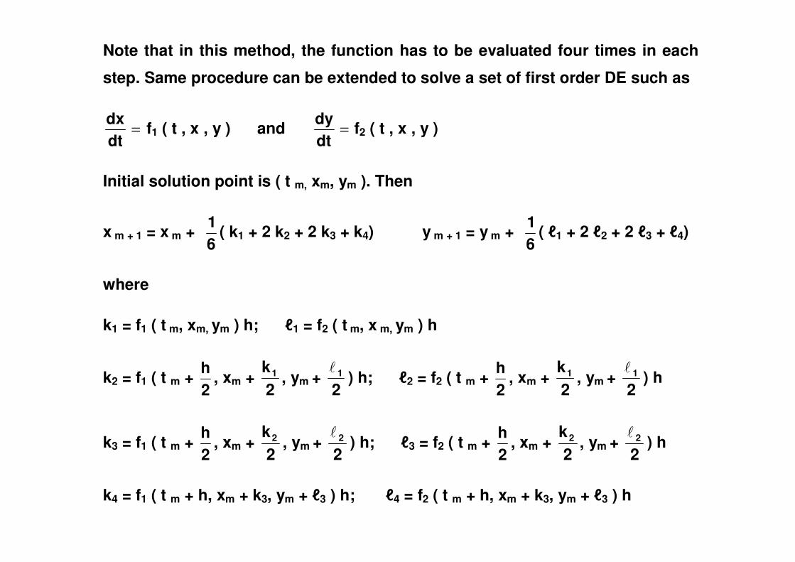
Note that in this method, the function has to be evaluated four times in each

step. Same procedure can be extended to solve a set of first order DE such as

=dtdx f1 ( t , x , y ) and =

dtdy f2 ( t , x , y )

Initial solution point is ( t m, xm, ym ). Then

x m + 1 = x m + 61 ( k1 + 2 k2 + 2 k3 + k4) y m + 1 = y m +

61 ( �1 + 2 �2 + 2 �3 + �4)

where where

k1 = f1 ( t m, xm, ym ) h; �1 = f2 ( t m, x m, ym ) h

k2 = f1 ( t m + 2h , xm +

2k1 , ym +

21� ) h; �2 = f2 ( t m +

2h , xm +

2k1 , ym +

21� ) h

k3 = f1 ( t m + 2h , xm +

2k2 , ym +

22� ) h; �3 = f2 ( t m +

2h , xm +

2k2 , ym +

22� ) h

k4 = f1 ( t m + h, xm + k3, ym + �3 ) h; �4 = f2 ( t m + h, xm + k3, ym + �3 ) h

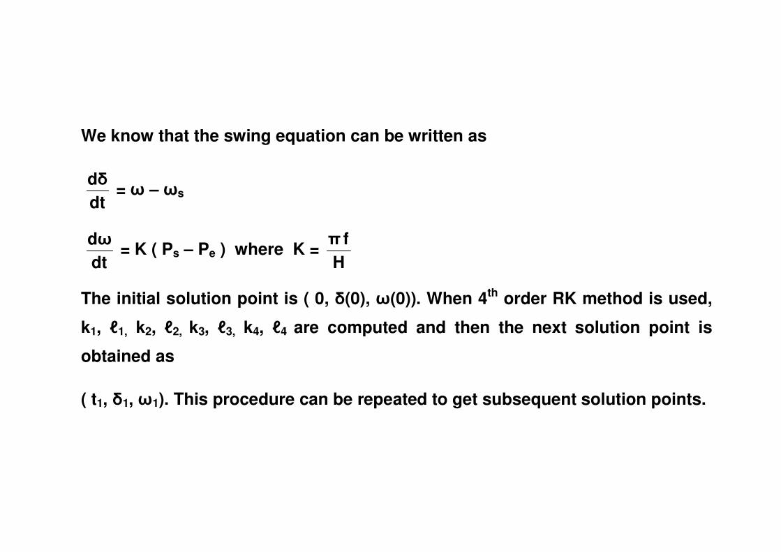
We know that the swing equation can be written as

dtd� = � – �s

dtd� = K ( Ps – Pe ) where K =

Hf�

The initial solution point is ( 0, �(0), �(0)). When 4th order RK method is used,

k1, �1, k2, �2, k3, �3, k4, �4 are computed and then the next solution point is

obtained as

( t1, �1, �1). This procedure can be repeated to get subsequent solution points.

Example 11

Consider the problem given in previous example and solve it using 4th order

RK method.

Solution

As seen in the previous example, two first order DEs are

d�Initial point is: �(0) = 0.2333 rad. �(0) = 314.1593 rad. / sec.

dtd� = � – 314.1593

dtd� = 39.2699 ( 1 – Pe )

During the first switching interval t = 0+ to 0.1 sec. electric output power Pe = 0.

)eP(139.2699dtd�

314.1593�dtd�

−=−=

Initial point is: �(0) = 0.2333 rad. �(0) = 314.1593 rad. / sec.

To calculate �(0.02) and �(0.02)

k1 = (314.1593 – 314.1593) x 0.02 = 0 �1 = 39.2699 ( 1 – 0 ) x 0.02 = 0.7854

�(0) + k1 / 2 = 0.2333; �(0) + �1 / 2 = 314.1593 + 0.3927 = 314.552

k2 = (314.552 – 314.1593) x 0.02 = 0.007854 �2 = 39.2699 ( 1 – 0 ) x 0.02 = 0.7854

�(0) + k2 / 2 = 0.2372; �(0) + �2 / 2 = 314.1593 + 0.3927 = 314.552

k = (314.552 – 314.1593) x 0.02 = 0.007854 � = 39.2699 ( 1 – 0 ) x 0.02 = 0.7854 k3 = (314.552 – 314.1593) x 0.02 = 0.007854 �3 = 39.2699 ( 1 – 0 ) x 0.02 = 0.7854

�(0) + k3 = 0.2412; �(0) + �3 = 314.1593 + 0.7854 = 314.9447

k4 = (314.9447 – 314.1593) x 0.02 = 0.0157 �4 = 39.2699 ( 1 – 0 ) x 0.02 = 0.7854

�(0.02) = 0.2333 + 61 [ 0 + 2 (0.007854) + 2 (0.007854) + 0.0157 ] = 0.24115 rad.

�(0.02) = 314.1593 + 61 [ 0.7854 + 2 (0.7854) + 2 (0.7854) + 0.7854 ]

= 314.9447 rad / sec.

Latest point is: �(0.02) = 0.24115 rad. �(0.02) = 314.9447 rad. / sec.

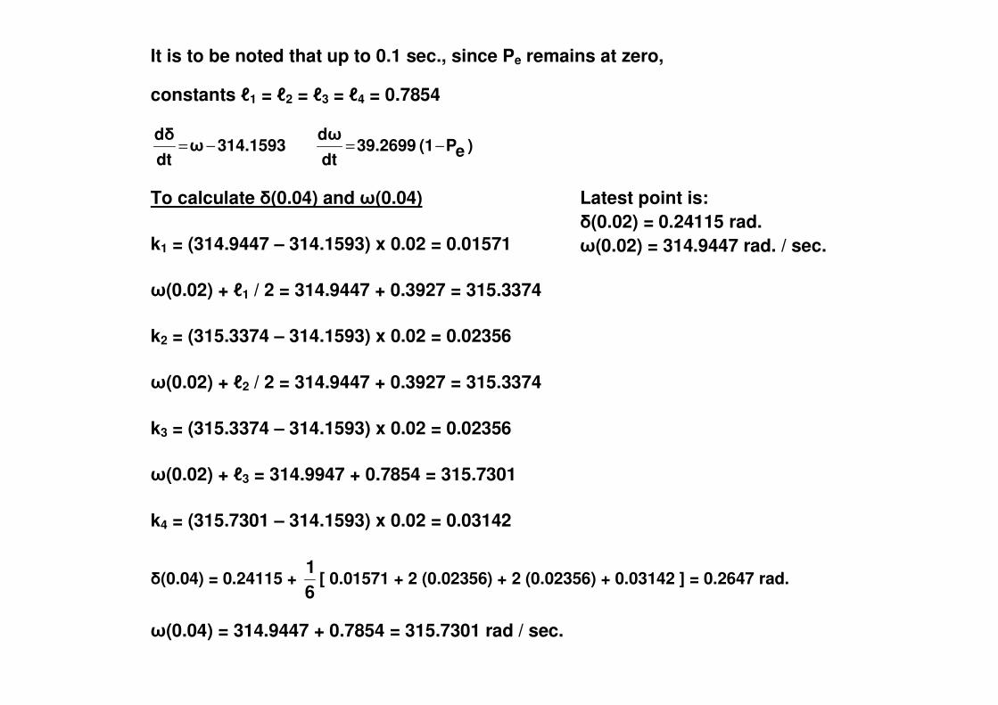
It is to be noted that up to 0.1 sec., since Pe remains at zero,

constants �1 = �2 = �3 = �4 = 0.7854

)eP(139.2699dtd�

314.1593�dtd�

−=−=

To calculate �(0.04) and �(0.04)

k1 = (314.9447 – 314.1593) x 0.02 = 0.01571

�(0.02) + �1 / 2 = 314.9447 + 0.3927 = 315.3374

k2 = (315.3374 – 314.1593) x 0.02 = 0.02356

�(0.02) + �2 / 2 = 314.9447 + 0.3927 = 315.3374

k3 = (315.3374 – 314.1593) x 0.02 = 0.02356

�(0.02) + �3 = 314.9947 + 0.7854 = 315.7301

k4 = (315.7301 – 314.1593) x 0.02 = 0.03142

�(0.04) = 0.24115 + 61

[ 0.01571 + 2 (0.02356) + 2 (0.02356) + 0.03142 ] = 0.2647 rad.

�(0.04) = 314.9447 + 0.7854 = 315.7301 rad / sec.

Latest point is: �(0.04) = 0.2647 rad. �(0.04) = 315.7301 rad. / sec.

)eP(139.2699dtd�

314.1593�dtd�

−=−=

To calculate �(0.06) and �(0.06)

k1 = (315.7301 – 314.1593) x 0.02 = 0.03142

�(0.04) + �1 / 2 = 315.7301 + 0.3927 = 316.1228

k2 = (316.1228 – 314.1593) x 0.02 = 0.03927

�(0.04) + �2 / 2 = 315.7301 + 0.3927 = 316.1228 �(0.04) + �2 / 2 = 315.7301 + 0.3927 = 316.1228

k3 = (316.1228 – 314.1593) x 0.02 = 0.03917

�(0.04) + �3 = 315.7301 + 0.7854 = 316.5155

k4 = (316.5155 – 314.1593) x 0.02 = 0.04712

�(0.06) = 0.2647 + 61 [ 0.03142 + 2 (0.03927) + 2 (0.03927) + 0.04712 ] = 0.304 rad.

�(0.06) = 315.7301 + 0.7854 = 316.5155 rad / sec.

Latest point is: �(0.06) = 0.304 rad. �(0.06) = 316.5155 rad. / sec.

)eP(139.2699dtd�

314.1593�dtd�

−=−=

To calculate �(0.08) and �(0.08)

k1 = (316.5155 – 314.1593) x 0.02 = 0.04712

�(0.06) + �1 / 2 = 316.5155 + 0.3927 = 316.9082

k2 = (316.9082 – 314.1593) x 0.02 = 0.05498

�(0.06) + �2 / 2 = 316.5155 + 0.3927 = 316.9082 �(0.06) + �2 / 2 = 316.5155 + 0.3927 = 316.9082

k3 = (316.9082 – 314.1593) x 0.02 = 0.05498

�(0.06) + �3 = 316.5155 + 0.7854 = 317.3009

k4 = (317.3009 – 314.1593) x 0.02 = 0.06283

�(0.08) = 0.2647 + 61 [ 0.04712 + 2 (0.05498) + 2 (0.05498) + 0.06283 ] = 0.359 rad.

�(0.08) = 316.5155 + 0.7854 = 317.3009 rad / sec.

Latest point is: �(0.08) = 0.359 rad. �(0.08) = 317.3009 rad. / sec.

)eP(139.2699dtd�

314.1593�dtd�

−=−=

To calculate �(0.1) and �(0.1)

k1 = (317.3009 – 314.1593) x 0.02 = 0.06283

�(0.08) + �1 / 2 = 317.3009 + 0.3927 = 317.6936

k2 = (317.6936 – 314.1593) x 0.02 = 0.07069

�(0.08) + �2 / 2 = 317.3009 + 0.3927 = 317.6936

k3 = (317.6936 – 314.1593) x 0.02 = 0.07069 k3 = (317.6936 – 314.1593) x 0.02 = 0.07069

�(0.08) + �3 = 317.3009 + 0.7854 = 318.0863

k4 = (318.0863 – 314.1593) x 0.02 = 0.07854

�(0.1) = 0.359 + 61 [ 0.06283 + 2 (0.07069) + 2 (0.07069) + 0.07854 ] = 0.4297 rad.

�(0.1) = 317.1593 + 0.7854 = 318.0863 rad. / sec.

At t = 0.1 sec., the fault is cleared. As seen in the previous example, for t 0.1

sec., electric power output of the alternator is given by Pe = 4.3261 sin �

To calculate �(0.12) and �(0.12)

k1 = (318.0863 – 314.1593) x 0.02 = 0.07854

Pe = 4.3261 sin (0.4297 rad.) = 1.8022

�1 = 39.2699 ( 1 – 1.8022 ) x 0.02 = - 0.63

�(0.1) + k1 / 2 = 0.4690; �(0.1) + �1 / 2 = 318.0863 - 0.315 = 317.7713

k2 = (317.7713 – 314.1593) x 0.02 = 0.07224

Pe = 4.3261 sin (0.469 rad.) = 1.9554

�2 = 39.2699 ( 1 – 1.9554 ) x 0.02 = - 0.7504

�(0.1) + k2 / 2 = 0.4658; �(0.1) + �2 / 2 = 318.0863 + 0.3752 = 317.7111

k3 = (317.7111 – 314.1593) x 0.02 = 0.07104

Pe = 4.3261 sin (0.4658 rad.) = 1.9430

�3 = 39.2699 ( 1 – 1.9430 ) x 0.02 = - 0.7406

�(0.1) + k3 = 0.5007; �(0.1) + �3 = 318.0863 - 0.7406 = 317.3457

k4 = (317.3457 – 314.1593) x 0.02 = 0.06373

Pe = 4.3261 sin (0.5007 rad.) = 2.0767

�4 = 39.2699 ( 1 – 2.0767 ) x 0.02 = - 0.8456

�(0.12) = 0.4297 + 61

[ 0.07854 + 2 (0.07224) + 2 (0.07104) + 0.06373 ] = 0.5012 rad.

�(0.12)= 318.0863 +61

[ - 0.63 - 2 (0.7504) - 2 (0.7406) - 0.8456 ]= 317.3434 rad. / sec.

Latest point is: �(0.12) = 0.5012 rad. �(0.12) = 317.3434 rad. / sec.

)eP(139.2699dtd�

314.1593�dtd�

−=−=

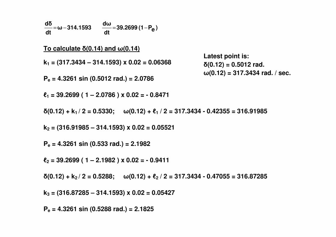
To calculate �(0.14) and �(0.14)

k1 = (317.3434 – 314.1593) x 0.02 = 0.06368

Pe = 4.3261 sin (0.5012 rad.) = 2.0786

�1 = 39.2699 ( 1 – 2.0786 ) x 0.02 = - 0.8471

�(0.12) + k1 / 2 = 0.5330; �(0.12) + �1 / 2 = 317.3434 - 0.42355 = 316.91985

k2 = (316.91985 – 314.1593) x 0.02 = 0.05521

Pe = 4.3261 sin (0.533 rad.) = 2.1982

�2 = 39.2699 ( 1 – 2.1982 ) x 0.02 = - 0.9411

�(0.12) + k2 / 2 = 0.5288; �(0.12) + �2 / 2 = 317.3434 - 0.47055 = 316.87285

k3 = (316.87285 – 314.1593) x 0.02 = 0.05427

Pe = 4.3261 sin (0.5288 rad.) = 2.1825

�3 = 39.2699 ( 1 – 2.1825 ) x 0.02 = - 0.9287

�(0.12) + k3 = 0.5555; �(0.12) + �3 = 317.3434 - 0.9287 = 316.4147

k4 = (316.4147 – 314.1593) x 0.02 = 0.04511

Pe = 4.3261 sin (0.5555 rad.) = 2.2814

�4 = 39.2699 ( 1 – 2.2814 ) x 0.02 = - 1.0064

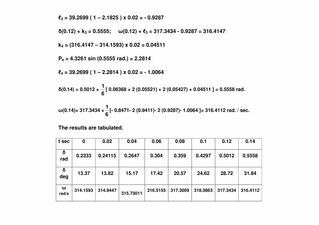
�(0.14) = 0.5012 + 61

[ 0.06368 + 2 (0.05521) + 2 (0.05427) + 0.04511 ] = 0.5558 rad.

�(0.14)= 317.3434 +61

[- 0.8471- 2 (0.9411)- 2 (0.9287)- 1.0064 ]= 316.4112 rad. / sec. �(0.14)= 317.3434 +6

[- 0.8471- 2 (0.9411)- 2 (0.9287)- 1.0064 ]= 316.4112 rad. / sec.

The results are tabulated.

t sec 0 0.02 0.04 0.06 0.08 0.1 0.12 0.14

� rad

0.2333 0.24115 0.2647 0.304 0.359 0.4297 0.5012 0.5558

� deg

13.37 13.82 15.17 17.42 20.57 24.62 28.72 31.84

� rad/s

314.1593 314.9447 315.73011

316.5155 317.3009 318.0863 317.3434 316.4112

�

MULTI MACHINE TRANSIENT STABILITY ANALYSIS

The equal area criterion cannot be used directly in systems having three or

more machines. Although the physical phenomena observed in the two-

machine problems basically reflect that of the multi-machine case, the

complexity of the numerical computations increases with the number of

machines considered.

For transient stability study, the system conditions before the fault occurs and

the network configuration for prefault, during the fault and post fault status

must be known. Consequently in the multimachine case the following four

phases of calculations are involved. phases of calculations are involved.

1. The steady state prefault conditions for the given system are calculated

using power flow program.

2. The network representation for transient stability study is arrived at by

suitable representing the generator reactances and loads.

3. The network representation obtained in step 2, is then modified to account

for the during fault and post fault conditions

4. Employing numerical technique swing equations of the machines can be

solved and the swing curves are obtained.

From the first phase of calculations we know the values of real power, reactive

power, and voltages at each generator terminal and load bus, with all angles

measured with respect to the slack bus.

The following are the assumptions commonly made in transient stability

studies.

(a) The mechanical power input to each machine remains constant during the

entire period of swing curve computation.

(b) Damping power is negligible.

(c) Each machine can be represented by a internal voltage source, behind a (c) Each machine can be represented by a internal voltage source, behind a

constant transient reactance as shown in Fig. 27. Magnitude of the internal

voltage remains constant while its phase angle changes in time.

��

Fig. 27 Synchronous Machine and its equivalent circuit

I

+

-

j xd’

| E’ | �∠ ,

��

V t

Knowing that

Vt I* = Pg + j Qg (41)

machine current is obtained as

I = *t

gg

V

QjP − (42)

Thus the internal voltage of generator is computed as Thus the internal voltage of generator is computed as

E’ = Vt + ( j Xd’ ) I (43)

By writing the internal voltage of generator as

E’ = | E’ | ∠� (44)

initial rotor angle � can be obtained.

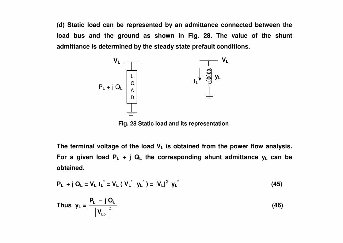
(d) Static load can be represented by an admittance connected between the

load bus and the ground as shown in Fig. 28. The value of the shunt

admittance is determined by the steady state prefault conditions.

VL

PL + j QL

VL

IL

Fig. 28 Static load and its representation

yL �

�

�

�

The terminal voltage of the load VL is obtained from the power flow analysis.

For a given load PL + j QL the corresponding shunt admittance yL can be

obtained.

PL + j QL = VL IL* = VL ( VL

* yL* ) = |VL|2 yL

* (45)

Thus yL = 2

Lp

LL

V

QjP − (46)

Fig. 28 Static load and its representation

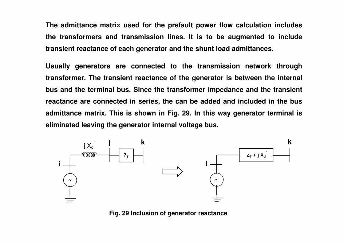
The admittance matrix used for the prefault power flow calculation includes

the transformers and transmission lines. It is to be augmented to include

transient reactance of each generator and the shunt load admittances.

Usually generators are connected to the transmission network through

transformer. The transient reactance of the generator is between the internal

bus and the terminal bus. Since the transformer impedance and the transient

reactance are connected in series, the can be added and included in the bus

admittance matrix. This is shown in Fig. 29. In this way generator terminal is

eliminated leaving the generator internal voltage bus. eliminated leaving the generator internal voltage bus.

Fig. 29 Inclusion of generator reactance

k j

i

��

��

j Xd’ k

i

��

������ �����

Loads are accommodated by adding the load admittances in the

corresponding diagonal elements in the bus admittance matrices. Note that

now the injected current is zero at all buses except the internal buses of the

generators. The network equations for system with three machines and two

load buses will be of the form

������

�

�

������

�

�

4544434241

3534333231

2524232221

1514131211

YYYYYYYYYYYYYYYYYYYYYYYYY

������

�

�

������

�

�

4

'3

'2

'1

VVEEE

=

������

�

�

������

�

�

003

2

1

III

(47)

���� 5554535251 YYYYY ��

�� 5V ���� 0

Since only the generator internal buses have injections, all other buses in the

bus admittance matrix can be eliminated by Kron reduction. The dimension of

the modified bus admittance matrix then corresponds to number of

generators. For three machine system network equations will be of the form

[Ybus] ���

�

�

���

�

�

'3

'2

'1

EEE

= ���

�

�

���

�

�

3

2

1

III

(48)

Similar to bus power equation in power flow analysis, now the power output of

generator i can be computed from

Pg i = |Ei’|2 Gii + )��(�cos|Y|EE inin

m

in1n

inn'

i' −+�

≠=

= |Ei’|2 Gii + )�(�cos|Y|EE nini

m

in1n

inn'

i' −�

≠=

(49)

where �in is the angle of Yin in equation (48) and �i�n = �i – �n�where �in is the angle of Yin in equation (48) and �i�n = �i – �n�

For example for the three machine system the power output of generator 1 is

given by

Pe 1 = |E1’|2 G11 + |E1

’| |E2’| |Y12| cos (�12 – �12) + |E1

’| |E3’| |Y13| cos (�13 – �13) (50)

The power-angle equations form part of the swing equations

ieim2

2

s

i PPdt�d

�

H 2−=

I = 1,2,3 (51)

Example 12

A 60 Hz, 230 kV transmission system shown in Fig. 30 has two generators of

finite inertia and an infinite bus. The transformer and line data are shown

inTable 1. Power flow results are shown in Table 2. Values are in per unit on

230 kV, 100 MVA base.

The generators have reactances and H values expressed on a 100 MVA base

as follows:

Generator 1: 400 MVA, 20 kV, Xd’ = 0.067 p.u. H = 11.2 MJ/MVA

Generator 2: 250 MVA, 18 kV, Xd’ = 0.10 p.u. H = 8.0 MJ/MVA

Fig. 30 One line diagram for Example 12

L5

Generator 2

5

��

��

��

1

2

4 3

Generator 1

L4 Infinite Bus

Table 1

Line and transformer data:

Bus to bus Series z Shunt Y R X B

Transformer 1 – 4 Transformer 2 – 5

0.022 0.040

Line 3 – 4 Line 3 – 5 (1) Line 3 – 5 (2) Line 4 - 5

0.007 0.008 0.008 0.018

0.040 0.047 0.047 0.110

0.082 0.098 0.098 0.226

�

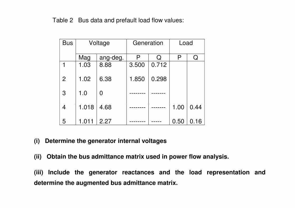
Table 2 Bus data and prefault load flow values:

Bus Voltage Generation Load

Mag ang-deg. P Q P Q 1 2 3 4

1.03 1.02 1.0 1.018

8.88 6.38 0 4.68

3.500 1.850 -------- --------

0.712 0.298 ------- -------

1.00

0.44

(i) Determine the generator internal voltages

(ii) Obtain the bus admittance matrix used in power flow analysis.

(iii) Include the generator reactances and the load representation and

determine the augmented bus admittance matrix.

4 5

1.018 1.011

4.68 2.27

-------- --------

------- -----

1.00 0.50

0.44 0.16

Solution

(i) Current supplied by the generators are:

I1 = *1

11

V

)Qj(P + = 08.88-1.03

0.712j3.5

∠−

= 3.468 ∠ - 2.6190

I2 = *

2

22

V

)Qj(P + = 06.38-1.02

0.298j1.85

∠−

= 1.837 ∠ - 2.7710

Thus

E1’ = V1 + j Xd1

’ I1 = 1.03 ∠ 8.88 + ( j 0.067 ) ( 3.468 ∠ - 2.6190 ) = 1.1 ∠ 20.820

E2’ = 1.02 ∠ 6.38 + ( j 0.1 ) ( 1.837 ∠ - 2.7710 ) = 1.065 ∠ 16.190

E3’ = 1.0 ∠ 0.00

(ii) Using the transformer and transmission lone data in Table 1, the bus

admittance matrix can be obtained as:

������

�

�

������

�

�

−+−+−+−−+−+−+−−

−−

j74.99768.4879j8.85381.4488j41.3557.0392j250j8.85381.4488j78.41155.6939j24.25714.2450j45.4545j41.3557.0392j24.25714.245j65.473211.284200

j2500j2500j45.454500j45.4545

(iii) To include reactance of generator 1:

Remove the transformer 1 – 4; Its admittance = - j45.4545

Add admittance of j45.4545 between 1 – 4.

Resulting bus admittance matrix will be

������

�

�

������

�

�

−+−+−+−−+−+−+−−

−

j74.99768.4879j8.85381.4488j41.3557.0392j250j8.85381.4488j32.9575.6939j24.25714.24500j41.3557.0392j24.25714.245j65.473211.284200

j2500j25000000

��

Admittance of series combination of generator reactance and transformer =

1/(j0.067 + j0.022) = - j 11.236

Add this admittance between buses 1 – 4. Resultant bus admittance matrix will

be

������

�

�

������

�

�

−+−+−+−−+−+−+−−

−

j74.99768.4879j8.85381.4488j41.3557.0392j250j8.85381.4488j44.1935.6939j24.25714.2450j11.236j41.3557.0392j24.25714.245j65.473211.284200

j2500j2500j11.23600j11.236-

�

To include reactance of generator 2:

Remove the transformer 2 – 5

Its admittance = - j25 Add admittance of j25 between 2 – 5.

Resulting bus admittance matrix will be

������

�

�

������

�

�

−+−+−+−−+−+−+−−

j49.99768.4879j8.85381.4488j41.3557.039200j8.85381.4488j44.1935.6939j24.25714.2450j11.236j41.3557.0392j24.25714.245j65.473211.284200

000000j11.23600j11.236-

Admittance of series combination of generator reactance and transformer =

1/(j0.1 + j0.04) = - j 7.1429

Add this admittance between buses 2 – 5. Resultant bus admittance matrix will

be

������

�

�

������

�

�

−+−+−+−−+−+−+−−

j57.14058.4879j8.85381.4488j41.3557.0392j7.14290j8.85381.4488j44.1935.6939j24.25714.2450j11.236j41.3557.0392j24.25714.245j65.473211.284200

j7.1429007.1429 j -00j11.23600j11.236-

�

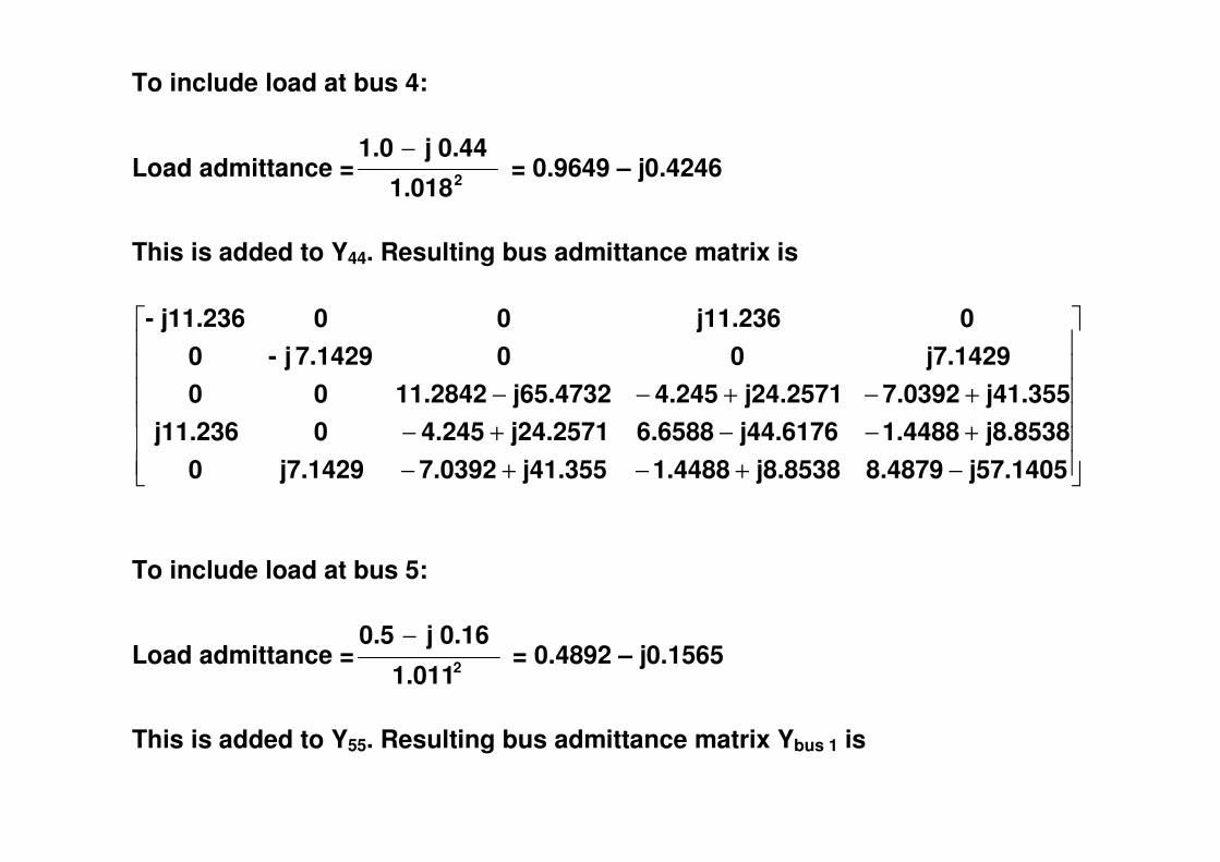
To include load at bus 4:

Load admittance = 21.018

0.44j1.0 − = 0.9649 – j0.4246

This is added to Y44. Resulting bus admittance matrix is

������

������

+−−+−+−+−−

j8.85381.4488j44.61766.6588j24.25714.2450j11.236j41.3557.0392j24.25714.245j65.473211.284200

j7.1429007.1429 j -00j11.23600j11.236-

��

���

� −+−+−+−−+−j57.14058.4879j8.85381.4488j41.3557.0392j7.14290

j8.85381.4488j44.61766.6588j24.25714.2450j11.236

To include load at bus 5:

Load admittance = 21.011

0.16j0.5 − = 0.4892 – j0.1565

This is added to Y55. Resulting bus admittance matrix Ybus 1 is

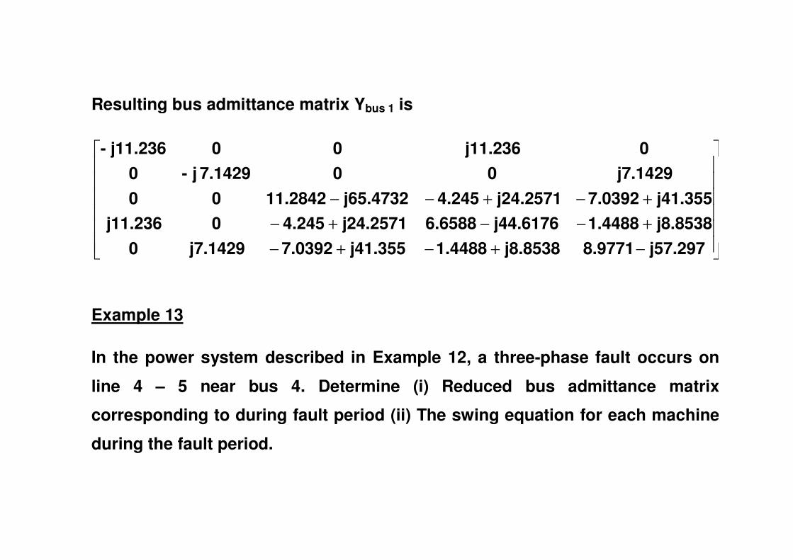
Resulting bus admittance matrix Ybus 1 is

������

�

�

������

�

�

−+−+−+−−+−+−+−−

j57.2978.9771j8.85381.4488j41.3557.0392j7.14290j8.85381.4488j44.61766.6588j24.25714.2450j11.236j41.3557.0392j24.25714.245j65.473211.284200

j7.1429007.1429 j -00j11.23600j11.236-

Example 13

In the power system described in Example 12, a three-phase fault occurs on

line 4 – 5 near bus 4. Determine (i) Reduced bus admittance matrix

corresponding to during fault period (ii) The swing equation for each machine

during the fault period.

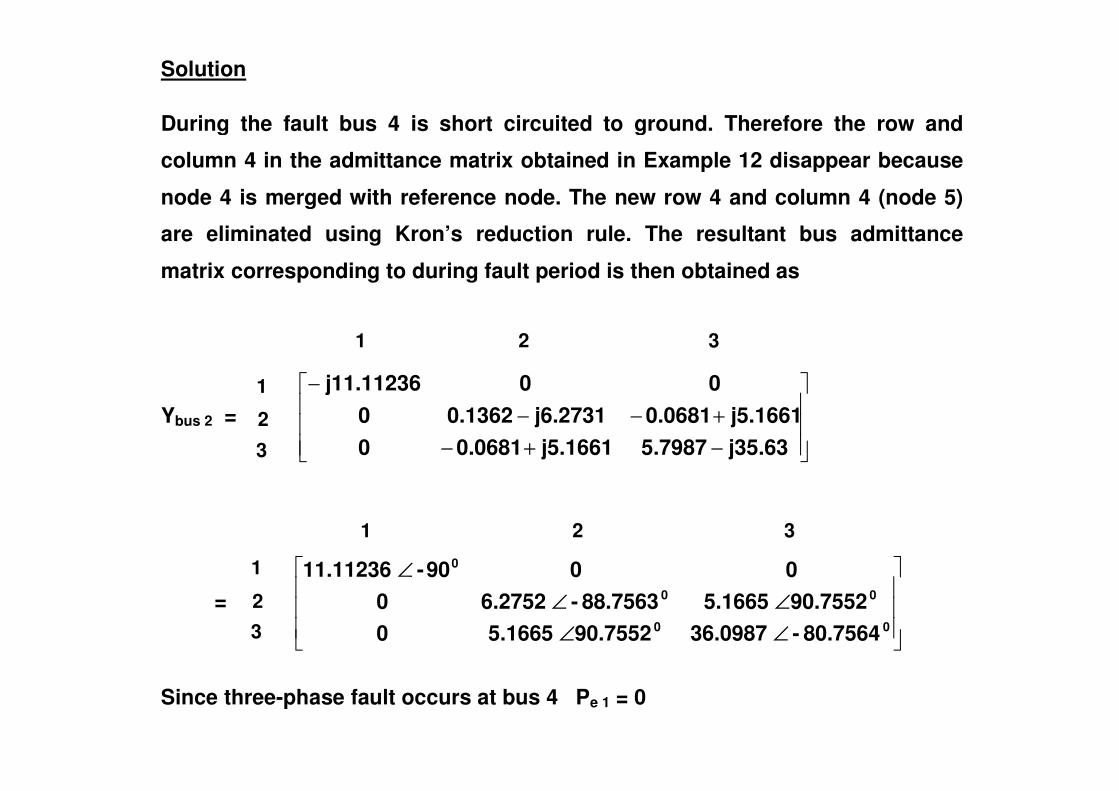
Solution

During the fault bus 4 is short circuited to ground. Therefore the row and

column 4 in the admittance matrix obtained in Example 12 disappear because

node 4 is merged with reference node. The new row 4 and column 4 (node 5)

are eliminated using Kron’s reduction rule. The resultant bus admittance

matrix corresponding to during fault period is then obtained as

��

��− 00j11.11236

1 2 3

1 Ybus 2 =

���

�

�

���

�

�

−+−+−−

j35.635.7987j5.16610.06810j5.16610.0681j6.27310.13620

= ���

�

�

���

�

�

∠∠∠∠

∠

00

00

0

80.7564- 36.098790.7552 5.1665090.7552 5.166588.7563- 6.275200090- 11.11236

Since three-phase fault occurs at bus 4 Pe 1 = 0

3

1

2

1 2 3

3

1

2

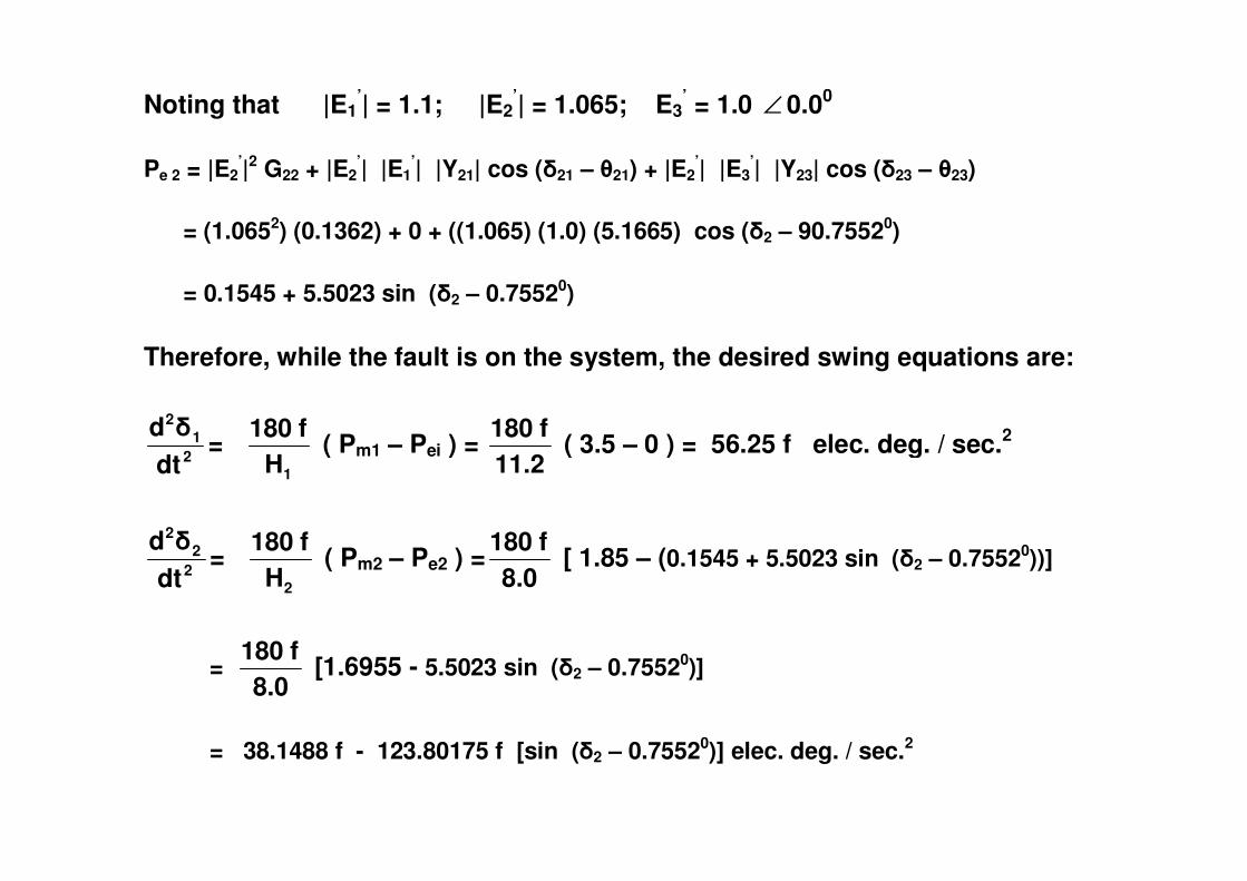
Noting that |E1’| = 1.1; |E2

’| = 1.065; E3’ = 1.0 ∠ 0.00

Pe 2 = |E2’|2 G22 + |E2

’| |E1’| |Y21| cos (�21 – �21) + |E2

’| |E3’| |Y23| cos (�23 – �23)

= (1.0652) (0.1362) + 0 + ((1.065) (1.0) (5.1665) cos (�2 – 90.75520)

= 0.1545 + 5.5023 sin (�2 – 0.75520)

Therefore, while the fault is on the system, the desired swing equations are:

12�d

= f 180 ( Pm1 – Pei ) = f 180 ( 3.5 – 0 ) = 56.25 f elec. deg. / sec.2 2

1

dt�d

= 1H

f 180

( Pm1 – Pei ) =

11.2f 180

( 3.5 – 0 ) = 56.25 f elec. deg. / sec.2

22

2

dt�d

= 2H

f 180

( Pm2 – Pe2 ) =

8.0f 180 [ 1.85 – (0.1545 + 5.5023 sin (�2 – 0.75520))]

= 8.0

f 180 [1.6955 - 5.5023 sin (�2 – 0.75520)]

= 38.1488 f - 123.80175 f [sin (�2 – 0.75520)] elec. deg. / sec.2

Example 14

The three-phase fault in Example 13 is cleared by simultaneously opening the

circuit breakers at the ends of the faulted line. Determine (i) the reduced bus

admittance matrix corresponding to the postfault period (ii) the swing

equations for the postfault period.

Solution

When the fault is cleared by removing line 4 – 5, the prefault Y matrix arrived When the fault is cleared by removing line 4 – 5, the prefault Ybus matrix arrived

at in Example 12, must be modified. Prefault Ybus is:

������

�

�

������

�

�

−+−+−+−−+−+−+−−

j57.2978.9771j8.85381.4488j41.3557.0392j7.14290j8.85381.4488j44.61766.6588j24.25714.2450j11.236j41.3557.0392j24.25714.245j65.473211.284200

j7.1429007.1429 j -00j11.23600j11.236-

�

Opening of line 4 – 5 whose admittance is 1/(0.018 + j 0.11) can be

implemented by adding admittance (– 1.4488 + j 8.8538) across 4 – 5 and

removing the half line charging admittance of j 0.113 Resulting matrix is

������

�

�

������

�

�

−+−−+−

+−+−−

j48.55627.52830j41.3557.0392j7.142900j35.87685.21j24.25714.2450j11.236

j41.3557.0392j24.25714.245j65.473211.284200j7.1429007.1429 j -0

0j11.23600j11.236-

Now using Kron’s elimination of node 4 and 5, bus admittance matrix

corresponding to the postfault period is then obtained as

Ybus 3 = ���

�

�

���

�

�

−+−++−−+−

j13.87281.3927j6.09750.09017.6291 j 0.2216 -j6.09750.0901j6.11680.159107.6291 j 0.2216 -0j7.89710.5005

= ���

�

�

���

�

�

∠∠∠∠∠∠

00

00

00

84.2672- 13.942690.8466 6.0982090.8466 6.098288.5101- 6.1189091.66387.6323086.3237- 7.8058

1 2 3

3

1

2

1 2 3

3

1

2

Noting that |E1’| = 1.1; |E2

’| = 1.065; E3’ = 1.0 ∠ 0.00

Pe 1 = |E1’|2 G11 + |E1

’| |E2’| |Y12| cos (�12 – �12) + |E1

’| |E3’| |Y13| cos (�13 – �13)

= (1.12) (0.5005) + 0 + ((1.1) (1.0) (7.6323) cos (�1 – 91.66380)

= 0.6056 + 8.3955 sin (�1 – 1.66380)

Pe 2 = |E2’|2 G22 + |E2

’| |E1’| |Y21| cos (�21 – �21) + |E2

’| |E3’| |Y23| cos (�23 – �23)

= (1.0652) (0.1591) + 0 + ((1.065) (1.0) (6.0982) cos (�2 – 90.84660)

= 0.1804 + 6.4934 sin (�2 – 0.84660)

Therefore, while the fault is on the system, the desired swing equations are:

21

2

dt�d

= 1H

f 180

( Pm1 – Pei ) =

11.2f 180

[ 3.5 - (0.6056 + 8.3955 sin (�1 – 1.66380))]

= 11.2

f 180

[2.8945 - 8.3955 sin (�1 – 1.66380)]

= 46.5188 f - 134.9277 f sin (�1 – 1.66380)] elec. deg. / sec.2

22

2

dt�d

= 2H

f 180

( Pm2 – Pe2 ) =

8.0f 180 [ 1.85 – (0.1804 + 6.4934 sin (�2 – 0.84660))]

= 8.0

f 180 [1.6696 - 6.4934 sin (�2 – 0.84660)]

= 37.566 f - 146.1015 f [sin (�2 – 0.84660)] elec. deg. / sec.2

Factors Affecting Transient Stability

The two factors mainly affecting the stability of a generator are

INERTIA CONSTANT H and TRANSIENT REACTANCE Xd’.

Smaller value of H:

Smaller the value of H means, value of M which is equal to H / � f is smaller.

As seen in the step by step method

�� (n) = �� (n – 1) + P )1n(a − (�t)2 �� (n) = �� (n – 1) +

M (�t)

the angular swing of the machine in any interval is larger. This will result in

lesser CCT and hence instability may result.

$

�

%�

& '(()*�+'(�)�

,-�.�

Larger value of Xd’:

As the transient reactance of the machine increases, Pmax decreases. This is

so because the transient reactance forms part of over all series reactance of

the system. All the three power output curves are lowered when Pmax is

decreased. Accordingly, for a given shaft power Ps, the initial rotor angle �0 is

increased and maximum rotor angle �m is decreased. This results in smaller

difference between �0 and �m as seen in Fig. 31.

Pre-fault output power

Fig. 31

�m 0�

Input power

Post-fault output power

During-fault output power

0� �m

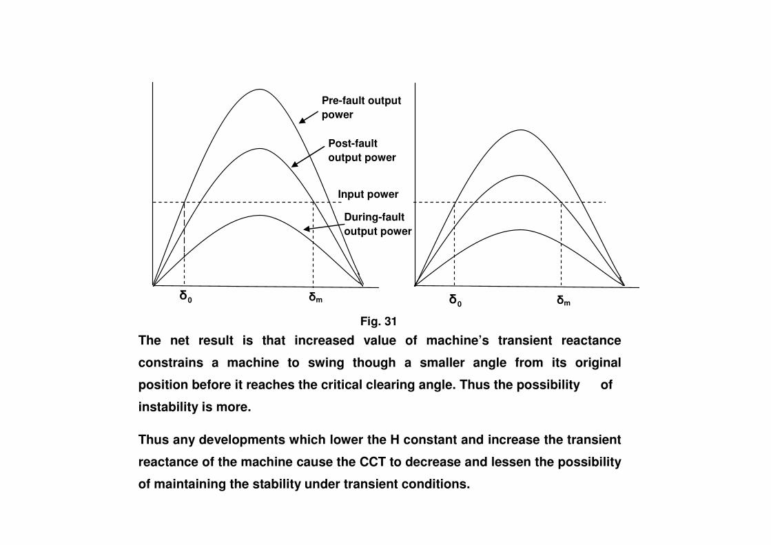
Input power

Post-fault output power

Pre-fault output power

During-fault output power

The net result is that increased value of machine’s transient reactance

constrains a machine to swing though a smaller angle from its original

position before it reaches the critical clearing angle. Thus the possibility of

instability is more.

Thus any developments which lower the H constant and increase the transient

reactance of the machine cause the CCT to decrease and lessen the possibility

of maintaining the stability under transient conditions.

Fig. 31

�m 0� 0� �m