NBER WORKING PAPER SERIES

UNDERSTANDING THE ECONOMIC IMPACT OF THE H-1B PROGRAM ONTHE U.S.

John BoundGaurav KhannaNicolas Morales

Working Paper 23153http://www.nber.org/papers/w23153

NATIONAL BUREAU OF ECONOMIC RESEARCH1050 Massachusetts Avenue

Cambridge, MA 02138February 2017

We would like to acknowledge the Alfred P. Sloan Foundation for generous research support. We thank Breno Braga, Gordon Hanson, Minjoon Lee, Rishi Sharma, Sebastian Sotelo, Sarah Turner and seminar participants at the NBER Global Talent SI Conference, University of California – San Diego, University of California – Davis and the University of Michigan for insightful comments and NE Barr for editorial assistance. The views expressed herein are those of the authors and do not necessarily reflect the views of the National Bureau of Economic Research.

NBER working papers are circulated for discussion and comment purposes. They have not been peer-reviewed or been subject to the review by the NBER Board of Directors that accompanies official NBER publications.

© 2017 by John Bound, Gaurav Khanna, and Nicolas Morales. All rights reserved. Short sections of text, not to exceed two paragraphs, may be quoted without explicit permission provided that full credit, including © notice, is given to the source.

Understanding the Economic Impact of the H-1B Program on the U.S.John Bound, Gaurav Khanna, and Nicolas MoralesNBER Working Paper No. 23153February 2017JEL No. J23,J24,J61

ABSTRACT

Over the 1990s, the share of foreigners entering the US high-skill workforce grew rapidly. This migration potentially had a significant effect on US workers, consumers and firms. To study these effects, we construct a general equilibrium model of the US economy and calibrate it using data from 1994 to 2001. Built into the model are positive effects high skilled immigrants have on innovation. Counterfactual simulations based on our model suggest that immigration increased the overall welfare of US natives, and had significant distributional consequences. In the absence of immigration, wages for US computer scientists would have been 2.6% to 5.1% higher and employment in computer science for US workers would have been 6.1% to 10.8% higher in 2001. On the other hand, complements in production benefited substantially from immigration, and immigration also lowered prices and raised the output of IT goods by between 1.9% and 2.5%, thus benefiting consumers. Finally, firms in the IT sector also earned substantially higher profits due to immigration.

John BoundDepartment of EconomicsUniversity of MichiganAnn Arbor, MI 48109-1220and NBERjbound@umich.edu

Gaurav KhannaUniversity of California, San Diegoand Center for Global Development gkhanna@cgdev.org

Nicolas MoralesUniversity of MichiganDepartment of EconomicsAnn Arbor, MI 48104moralesn@umich.edu

An increasingly high proportion of the scientists and engineers in the US were born abroad.

At a very general level, the issues that come up in the discussion of high-skill immigration

mirror the discussion of low-skill immigration. The most basic economic arguments suggest

that both high-skill and low-skill immigrants: (1) impart benefits to employers, to owners of

other inputs used in production such as capital, and to consumers, and (2) potentially, impose

some costs on workers who are close substitutes (Borjas, 1999). Evidence suggests, however,

that the magnitude of these costs may be substantially mitigated if US high-skill workers have

good alternatives to working in sectors most impacted by immigrants (Peri et al., 2013; Peri

and Sparber, 2011). Additionally, unlike low-skill immigrants, high-skill immigrants contribute

to the generation of knowledge and productivity through patenting and innovation, both of

which serve to shift out the production possibility frontier in the US and may also slow the

erosion of the US comparative advantage in high tech (Freeman, 2006; Krugman, 1979).

In this paper we study the impact that the recruitment of foreign computer scientists on H-1B

visas had on the US economy during the Internet boom of the 1990s. An H-1B is a non-

immigrant visa allowing US companies to temporarily employ foreign workers in specialized

occupations. The number issued annually is capped by the federal government. During the

1990s, we observe a substantial increase in the number of H-1B visas awarded to high-skill

workers, with those in computer-related occupations becoming the largest share of all H-1B

visa holders (U.S. General Accounting Office, 2000). Given these circumstances, it is of consid-

erable interest to investigate how the influx of H-1B visa holders during this period might have

affected labor market outcomes for US computer scientists and other US workers, and overall

productivity in the economy.

We focus on the period 1994 to 2001 for a number of reasons. During the latter half of the

1990s, the US economy experienced a productivity growth attributable, at least in part, to the

IT boom, facilitated by the influx of foreign talent (Jorgenson et al., 2015). At the same time,

the recruitment of H-1B labor by US firms was at or close to the H-1B cap during this period,

enabling us to treat foreign supply as determined by the cap. Finally, more recent growth of the

IT sector in India and changes in the law authorizing the H-1B have complicated the picture

since 2001.1

In earlier work evaluating the impact of immigration on Computer Science (CS) domestic

workers, we constructed a dynamic model that characterizes the labor supply and demand for

CS workers during this period (Bound et al., 2015). We built into the model the possibility that

labor demand shocks, such as the one created by the Internet boom, could be accommodated

by three sources of CS workers: recent college graduates with CS degrees, US residents in

different occupations who switch to CS jobs, and high-skill foreigners. Furthermore, our model

assumed firms faced a trade-off when deciding to employ immigrants: foreigners were potentially

either more productive or less costly than US workers, but incurred extra recruitment/hiring

1See Khanna and Morales (2015) for a long-run extension of this work that also models the Indian IT sector.

2

costs.

The approach we took in that analysis was distinctly partial equilibrium in nature – that is,

we focused on the market for computer scientists and ignored any wider impacts that high-skill

immigration might have on the US economy (Nathan, 2013). While we believe that approach

could be used to understand the impact that the availability of high-skill foreign labor might

have had for this market, it precludes any analysis of the overall welfare impact of the H-1B

program in particular, or of high-skill immigration more generally.

The implications of the model regarding the impact of immigration on the employment and

wages of native workers depended on the elasticity of labor demand for computer scientists.

As long as the demand curve sloped downwards, the increased availability of foreign computer

scientists would put downward pressure on the wages for computer scientists in the US. However,

in the case of computer scientists, other factors may affect this relationship. First, even in a

closed economy, the contribution of computer scientists to innovation reduces the negative

effects foreign computer scientists might have on the labor market opportunities for native

high-skill workers. In addition, in an increasingly global world, US restrictions on the hiring

of foreign high-skill workers are likely to result in greater foreign outsourcing work by US

employers. Indeed, if computer scientists are a sufficient spur to innovation, or if domestic

employers can readily offshore CS work, any negative effects that an increase in the number of

foreign CS workers might have on the domestic high-skill workforce would be offset by increases

in the domestic demand for computer scientists.

In Bound et al. (2015), we used data on wages, domestic and foreign employment, and under-

graduate degree completions by major, during the late 1990s and early 2000s to calibrate the

parameters of our model to reproduce the stylized facts of the CS market during the analytic

period (1994 to 2001). Next, we used the calibrated model to simulate counterfactuals on how

the economy would have behaved if firms had been restricted in the number of foreign CS

workers they could hire to the 1994 level. Conditional on our assumptions about the elasticity

of the demand curve for computer scientists, our simulation suggests that had US firms faced

this restriction, CS wages and the number of Americans working in CS and the enrollment

levels in US computer science programs would have been higher, but the total number of CS

workers in the US would have been lower.

The predictions of our model did not depend on the specific choice we made for non-calibrated

parameters, with one important exception: crowd out in the market for computer scientists

depended crucially on the elasticity of demand for their services. Ideally, we would have been

able to use exogenous supply shifts to identify the slope of the demand curve for computer

scientists, as we use exogenous shifts in demand to identify supply curves. In other contexts,

researchers have treated the increase in foreign born workers in the US economy as exogenous.

However, in the current context, immigration law in the US implies that most of the foreign

3

born and trained individuals who migrate to the US to work as computer scientists do so

because they are sponsored by US based firms. Thus, it seems implausible to treat the number

of foreign born computer scientists in the US as an exogenous increase in supply. In the end,

without credible sources of identifying information, we resorted to parametrically varying the

elasticity of the demand for computer scientists.

In the current analysis, we take a different track. We interpret the arguments about the

potential productivity effects of high-skill immigrants in terms of models of endogenous technical

change. Within the context of a simple general equilibrium model of the US economy, we link

productivity increases in the U.S. economy during the 1990s to increases in the utilization of

computer scientists in the economy. This allows us to derive the demand curve for computer

scientists.

Within the context of our model, it is possible to understand the effect that the availabil-

ity of high-skill foreign workers has on the earnings of both high and low-skill workers, the

goods available in the economy, and profits in the high-tech sector of the economy. However,

our conclusions are dependent both on our modeling choices and on values of our calibrated

parameters. For this reason, we do extensive sensitivity analyses to determine which of our

conclusions are robust.

A key feature of high-skill immigrants is that they contribute to innovation. While this point

is well understood, we know of no earlier work that has tried to quantify the magnitude of this

effect within the context of an explicit model of the US economy. The magnitude of this effect

is important because it speaks to the magnitude of any first-order gains to US residents of

high-skill immigration, and because it has a direct influence on the slope of the labor demand

curve for close substitutes for high-skill immigrants.

Our model is limited in a number of important respects. While we allow for endogenous

technical change, we incorporate trade in a very stylized manner and do not allow explicitly

for outsourcing.2 As such, we think our model captures relatively short-run effects of H-1B

immigration. Although in this sense our model is different from models incorporated in recent

work by, for example, Grossman and Rossi-Hansberg (2008) or di Giovanni et al. (2015), we

believe that it captures important elements of the current debate about the H-1B program.

We review this literature in detail, and describe the market for CS workers in section 1. Section

2 presents the model we build to characterize the market for CS workers when firms can recruit

foreigners. In section 3, we describe how we calibrate the parameters of the model and in section

4 we run counterfactual simulations where firms have restrictions on the number of foreigners

they can hire. Section 5 talks about welfare changes under this counterfactual scenario. We

conclude with section 6, which presents a discussion based on the results of the analysis.

2Available evidence suggests that outsourcing options were somewhat limited during the 1990s (Liu andTrefler, 2008), though it is not clear that this is still true.

4

1 The Market for Computer Scientists in the 1990s

1.1 The Information Technology Boom of the Late 1990s

The mid 1990s marks the beginning of the use of the Internet for commercial purposes in the

United States, and a concomitant jump in the number of Internet users. One indicator of a

contemporaneous increase in demand for IT workers is the rise of R&D expenditures among

firms providing computer programming services, and computer-related equipment. Specifically,

the share of total private R&D expenditures for firms in these sectors increased from 19.5% to

22.1% between 1991 and 1998.3 The entry and then extraordinary appreciation of tech firms

like Yahoo, Amazon, and eBay provide a further testament to the boom in the IT sector prior

to 2001.

These changes had a dramatic effect on the labor market for computer scientists. According

to the Census, the number of employed individuals working either as computer scientists or

computer software developers increased by 161% between the years 1990 and 2000. In compar-

ison, during the same period, the number of employed workers with at least a bachelor degree

increased by 27% and the number of workers in other science, technology, engineering, and

math (STEM) occupations increased by 14%.4 Table 1 shows that computer scientists as a

share of the college-educated workforce and the college-educated STEM workforce was rising

before 1990, but increased dramatically during the 1990s. Indeed, by 2000 more than half of

all STEM workers were computer scientists. In Figure 1a, we use CPS data to show a similar

pattern, additionally showing that the growth of CS employment started in the second half of

the decade - a period corresponding to the dissemination of the Internet.

The Internet innovation affected educational choices as well as employment decisions. We show

in Figure 1b that the CS share of both all bachelor’s degrees and of STEM major degrees

increased dramatically during this period, in both cases rising from about 2% of all Bachelor

degrees granted in 1994 to almost than 3.5% in 2001.

The behavioral response would be different if the boom was only temporary and respond to the

Y2K bug. The employment and educational evidence, however, suggests that many expected

this boom, as a response to technological innovations, to be permanent. Indeed, in 1997, the

Bureau of Labor Statistics (BLS) projected a steady increase in CS employment after the turn

of the century. More specifically, the BLS predicted that between 1996 and 2006 “Database

administrators, computer support specialists, and all other computer scientists” would be the

fastest growing occupation and “Computer engineers” would be the second fastest in terms of

3Bound et al. (2015) calculation using Compustat data4Here and elsewhere, our tabulations restrict the analysis to workers with at least a bachelor degree and use

the IPUMS suggested occupational cross walk. Other STEM occupations are defined as engineers, mathemati-cians and computer scientists. For more details see Appendix A.1.

5

jobs. Furthermore, they predicted that “Computer and data processing services” would grow

by 108% – the fastest growing industry in the country.5

In addition to affecting employment and enrollment decisions, there is also empirical evidence

that CS wages responded to expanding Internet use. From the Census, we observe an 18%

increase in the median real weekly wages of CS workers between 1990 and 2000. The CPS

presents similar patterns: starting in the year 1994 we observe in Figure 1c that wages of

computer scientists increased considerably when compared to both workers with other STEM

occupations and all workers with a bachelor degree. In fact, while during the beginning of the

1990s, the earnings of CS workers were systematically lower than other STEM occupations, the

wage differential tends to disappear after 1998.

1.2 Contribution of Immigration to the Growth of the High Tech

Workforce

Employment adjustments in the market for computer scientists occurred disproportionately

among foreigners during the Internet boom. Evidence for this claim is found in Table 1 and

Figure 1d, where we use Census and CPS data to compare the share of foreign computer

scientists to the share of foreign workers in other occupations.6 In the second half of the 1990s,

the foreign fraction of CS workers increased considerably more than both the foreign fraction of

all workers with a bachelor degree and the foreign fraction of all workers in a STEM occupation.

In particular, in 1994 the share of foreigners working in CS was about the same as the share

working in other STEM occupations, but later in the decade, during the boom in Internet use,

the share of foreigners among all CS workers rose steeply, comprising about 30% of the increase

in all CS workers during this period.

The growth in the representation of the foreigners among the US CS workforce was fueled by two

supply-side developments in this period. First, the foreign pool of men and women with college

educations in science and engineering fields increased dramatically (Freeman, 2009). In India,

an important source of CS workers in the US, the number of first degrees conferred in science

and engineering rose from 176,000 in 1990 to 455,000 in 2000. Second, the Immigration Act of

1990 established the H-1B visa program for temporary workers with at least a bachelor’s degree

working in “specialty occupations” including engineering, mathematics, physical sciences, and

business among others.

Firms wanting to hire foreigners on H-1B visas must first file a Labor Condition Application

(LCA) in which they attest that the firm will pay the visa holder the greater of the actual

compensation paid to other employees in the same job or the prevailing compensation for

5Source: BLS Employment Projections http : //www.bls.gov/news.release/history/ecopro 082498.txt6Here and elsewhere, we define foreigners as those who immigrated to the US after the age of 18. We believe

that this definition is reasonable proxy for workers who arrived to the US on non immigrant visas.

6

that occupation, and the firm will provide working conditions for the visa holder that do not

adversely affect the working conditions of the other employees. At that point, prospective H-

1B non-immigrants must demonstrate to the US Citizenship and Immigration Services Bureau

(USCIS) in the Department of Homeland Security (DHS) that they have the requisite education

and work experience for the posted positions. The USCIS may approve the petition for the H-

1B holder for a period of up to three years, with the possibility of a three-year extension. Thus

foreign workers can stay a maximum of six years on an H-1B visa, though firms can sponsor

these workers for a permanent resident visa. Because H-1B visas are approved for solely the

applying firm, H-1B foreign workers are effectively tied to their sponsoring company.

Since 1990, when the visa was initiated, the number of H-1B visas issued annually has been

capped. The initial cap was of 65,000 visas per year was not reached until the mid-1990s, when

demand began to exceed the cap. However, the allocation tended to fill each year on a first

come, first served basis, resulting in frequent denials or delays on H-1Bs because the annual cap

had been reached. After lobbying by the industry, Congress raised the cap first to 115,000 for

FY1999 and then to 195,000 for FY2000-2003, after which the cap reverted to 65,000. Figure

1e shows the growth in the number of H-1 visas (the H-1 was the precursor to the H-1B) issued

1976-2008, estimates of the stock of H-1 visas in the economy each year, and the changes in

the H-1B visa cap.7

Through the decade of the 1990s, foreign workers with H-1B visas became an important source

of labor for the technology sector. The National Survey of College Graduates shows that 55%

of foreigners working in CS fields in 2003 arrived in the US on an H-1B or a student-type

visa (F-1, J-1). Furthermore, institutional information indicates a significant increase in the

number of visas awarded to workers in computer-related occupations during the 1990s. A

1992 U.S. General Accounting Office report shows that “computers, programming, and related

occupations” corresponded to 11% of the total number of H-1 visas in 1989, while a report from

the U.S. Immigration and Naturalization Service (2000) finds that computer-related occupations

accounted for close to two-thirds of the H-1B visas awarded in 1999. More specifically, the

U.S. Department of Commerce (2000) estimated that during the late 1990s, 28% of all US

programmer jobs went to H-1B visa holders.

While H-1B visa holders represent an important source of computer scientists, they do not

represent all foreigners in the country working as computer scientists. A significant number of

such foreigners are permanent immigrants, some of whom may have come either as children

or as students. Other foreigners enter the US to work as computer scientists in the US on

7The Immigration and Nationality Act of 1952 established the precursor to the H-1B visa, the H-1. The H-1non-immigrant visa was targeted at aliens of “distinguished merit and ability” who were filling positions thatwere temporary. Non-immigrants on H-1 visas had to maintain a foreign residence. The Immigration Act of1990 established the main features of H-1B visa as it is known today, replacing “distinguished merit and ability”with the “specialty occupation” definition. It also dropped the foreign residence requirement and added a dualintent provision, allowing workers to potentially transfer from an H-1B visa to immigrant status.

7

L-1B visas, which permit companies with offices both in the US and overseas to move skilled

employees from overseas to the US. While we know of no data showing the fraction of computer

scientists working in the US on L-1B visas, substantially fewer L-1(A&B) visas are issued than

are H-1Bs.8

1.3 Impact of Immigrants on the High Tech Workforce in the US

Critics of the H-1B program (Matloff, 2003) argue that firms are using cheap foreign labor

to undercut and replace skilled US workers, although even the fiercest critics do not claim

that employers are technically evading the law (Kirkegaard, 2005). Rather, they argue that

firms skirt the requirement to pay H-1B visa holders prevailing wages by hiring over-qualified

foreigners into positions with low stated qualifications and concomitant low “prevailing wages.”

These critics claim that the excess supply of highly qualified foreigners willing to take the jobs

in the US plus the lack of portability of the H-1B visa limit the capacity of H-1B workers to

negotiate fair market wages.

One way to get a handle on the extent to which H-1B visa holders are being under-paid relative

to their US counterparts is to compare foreigners on H-1B visas to those with green cards – an

immigrant authorization allowing the holder to live and work in the US permanently, with no

restrictions on occupation. Using difference-in-difference propensity score matching and data

from the 2003 New Immigrant Survey, Mukhopadhyay and Oxborrow (2012) find that green

card holders earn 25.4 percent more than observably comparable temporary foreign workers.

Using log earnings regressions and data from an internet survey, Mithas and Lucas (2010)

find that IT professionals with green cards earn roughly 5 percent more than observationally

equivalent H-1B visa holders. Comparisons between green card and H-1B holders are far from

perfect. Since many green card holders begin as H-1B visa holders who are eventually sponsored

by their employers for permanent residence status, it is reasonable to assume that green card

holders are positively selected on job skills. Given this consideration, it is somewhat surprising

that the observed green card premium is not larger than this 5%.

Perhaps the most compelling work concerning productivity differences between H-1B visa hold-

ers and their US resident counterparts comes from a recent paper by Doran et al. (2015) who

analyze H-1B lotteries used in FY 2006 and 2007 to identify the productivity effects on firms

of hiring an additional H-1B worker. During these two years, firms that submitted an LCA

during the day the H-1B quota was hit would enter a lottery to determine whether they were

permitted to hire the additional H-1B worker. Doran et al. (2015) find that winning the lottery

had no effect on subsequent patenting or employment in the affected firm, consistent with the

notion that a firm unable to hire a H-1B worker would end up hiring an alternative, equally

8See Yeaple (2016) for a discussion on L-1 and H-1B visas.

8

productive worker.9

While there may be no incontrovertible estimate of the productivity (conditional on earnings)

advantage of foreign high-skill labor, simple economic reasons suggest this advantage must

exist. US employers face both pecuniary and non-pecuniary costs associated with hiring for-

eigners. A small GAO survey (U.S. General Accounting Office, 2011) estimated the legal and

administrative costs associated with each H-1B hire to range from $2,300 to $7,500 dollars.

Assuming that these workers earn $60,000 per year in total compensation, which would seem

to be conservative, this amounts to no more than 2% of compensation spread over 6 years. It

seems reasonable to assume that employers must expect some cost or productivity advantage

when hiring foreigners, however modest. If not, why would they incur the associated effort and

expense?

Whatever the perceived cost or productivity advantages, H-1B critics argue that US employers’

use of foreign labor in high-skill jobs either “crowds out” native workers from these jobs or puts

downward pressure on their wages. Although, as far as we know, critics of the H-1B program

have not yet estimated the magnitude of either of these effects, recent work by economists has

started to fill this void. Kerr and Lincoln (2010) and Hunt and Gauthier-Loiselle (2010) provide

original empirical evidence on the link between variation in immigrant flows and innovation

measured by patenting, finding evidence that the net impact of immigration is positive rather

than simply substituting for native employment. Kerr and Lincoln (2010) also show that

variation in immigrant flows at the local level related to changes in H-1B flows do not appear

to adversely impact native employment and have a small, statistically insignificant, effect on

their wages. More recently, Peri et al. (2014) found positive effects of high-skill immigrant

workers on the employment and wages of college-educated domestic workers.

A potential issue with the analyses of Kerr and Lincoln (2010) and Peri et al. (2014) is that

the observed, reduced-form outcomes may capture concurrent changes in area specific demand

for computer scientists. To circumvent the problem, each paper constructed a variable that

interacts an estimate for the total number of individuals working on H-1B visas in a city with

local area dependencies on H-1Bs.10 However, given the nature of the H-1B visa, the location

of immigrants depends, in large part, on the location of employers hiring them. If because of

local agglomeration effects, the IT boom was concentrated in areas of the country that were

already IT intensive (such as Silicon Valley), then the measure of local dependency would be

9Doran et al. (2015) point estimates suggest that replacing a US resident with a H-1B holder might raisepatenting at small firms by 0.26% (95% CI -0.42 0.47%), implying that the H-1Bs visa holders are no morethan 4.7% more productive than are US resident workers.

10Kerr and Lincoln (2010) and Peri et al. (2014) hope that the variation in this variable is driven largely bychanges in the cap on new H-1B visas that occurred over the last 20 years. That said, it is unclear the extentto which the variation they use is being driven by variation in the visa cap. Because of the dot com bubblebust in 2000 and 2001, the variation in the H-1B cap is only loosely related to actual number of H-1Bs issued.What is more, the cap will have different effects across areas, and one can worry about the exogeneity of thisvariation. In addition, it is hard to imagine that the cap was exogenous to the demand for IT workers.

9

endogenous, an issue that Kerr and Lincoln (2010) and Peri et al. (2014) understand.

Ghosh et al. (2014) take a different approach. They match all LCAs, with firm-level data on

publicly traded US companies, comparing changes in labor productivity, firm size, and profits

between 2001 and 2006, for firms that were highly dependent on H-1B labor with firms that were

not. They argue that the H-1B-dependent firms would feel more effects than their counterparts

from the dramatic drop in the H-1B cap from 195,000 to 65,000 in 2004. And, indeed, they

find that, over this period, labor productivity, firm size, and profits all declined more for the

H-1B-dependent firms, which they attribute to the loss of the H-1B labor. The concern here is

that the firms more dependent in H-1B labor in 2001 would have been systematically different

from those less so dependent in ways correlated with the change in performance between 2001

and 2006.

In another paper, Peri et al. (2015) use data on the number of LCAs filed by firms in local

(metro) areas during 2007 and 2008 as a measure of potential demand for H-1B workers, and

the number of H-1B applications filed by foreigners as their measure of H-1Bs hired. In 2007

and 2008, the number of H-1B applications exceeded the annual quotas, and lotteries were used

in awarding visas. The large gap between these two measures represent the unmet demand for

skilled foreign workers. Cross-metro-area variation in this variable is due to at least two sources:

(1) cross-metro-area demand for foreign high-skill labor, and (2) truly random fluctuations in

the fraction of LCAs picked in the lotteries. While this second source of variation should be

truly random, Peri et al. (2015) find too little of such variation to reliably identify the net

effects of high-skill labor immigration.

Previous researchers studying the impact of H-1B workers on the US economy have focused

on identifying exogenous variation in the number of H-1B workers, typically finding that H-

1B workers tend to raise productivity and act as complements to, rather than crowd-out,

college-educated native workers. However, as these researchers have acknowledged, it is easy

to question the validity of the instruments used in these analyses. Rather than using a natural

experiment to identify effects, we derive effects from a calibrated model. The model allows us

to connect endogenous productivity advances in the IT sector during the 1990s to changes in

the demand for CS labor. While the validity of the conclusions that Kerr and Lincoln (2010),

Peri et al. (2014), Peri et al. (2015), and Ghosh et al. (2014) depend on the validity of the

natural experiments they use to identify effects, our conclusions depend on our model accurately

reflecting key features of the US economy. As such, the credibility of our results hinges on the

plausibility of our assumptions and/or the robustness of our conclusions to variations in the

specific modeling choices we made.

10

2 A Model of the Product and Labor Markets

Our model consists of two major sections. The first is the product market where goods are

produced by firms and sold to consumers. The second is the labor market for college graduates,

where US workers decide whether to work as computer scientists or in other occupations. Our

product market, has two sectors: the IT sector and the ‘Other’ sector. The IT sector is monop-

olistically competitive, wherein firms produce different varieties of the same IT good. Firms

in the IT sector are heterogeneous in terms of their level of productivity, which is exogenously

drawn. Importantly, we include the possibility of endogenous technological change, whereby

CS workers’ innovation causes the production function to be increasing returns to scale at the

aggregate level. All other goods in the economy are produced in the residual ‘Other’ sector,

which is a perfectly competitive sector with homogeneous firms.

Every period a firm chooses its inputs to maximize profits. Since firms in the IT sector are

monopolistically competitive, they have some market power when making these choices. Firms

use intermediate inputs from the Other sector and labor to produce their output. The labor

inputs consist of three types of workers: computer scientists, college-educated non-computer

scientists, and non-college-educated workers. In our model, all foreign immigrants are hired as

computer scientists. IT sector firms are also able to export their products to foreign markets,

whereas the US economy imports only non-IT goods. Consumers, on the other hand, choose

how much of each good to consume in order to maximize their utility subject to their labor

income. Like firms, they make these choices every period, and have no savings.

Building on this setup, we include the labor supply decisions of college graduates. Since human

capital investments and career choices have long term payoffs, US workers in our model are

allowed to choose their fields of study and occupations based on the information they have

today and their expected payoffs in the future. They are then allowed to switch occupations,

by paying a switching cost, when a change occurs in the current or expected payoffs associated

with any occupation. Given the labor supply decisions of US workers, the labor supply of

immigrants, and the labor demand from firms in each sector, the market clears to determine

the equilibrium wages for each type of worker. Equilibrium prices are determined in the product

market, where the demand for the two types of goods from consumers meets the supply of these

goods from firms.

2.1 Product Market

2.1.1 Household problem

There are X number of consumers in the economy who supply one unit of labor each. Each

consumer has the same preferences over the two goods: Cd produced by the IT sector and Yd,

11

the good produced by the residual sector in the economy. Their preferences can be represented

by the Constant Elasticity of Substitution (CES) utility function in equation 1.

U(Cd, Yd) =[γC

σ−1σ

d + (1− γ)Yσ−1σ

d

] σσ−1

(1)

Yd is assumed to be homogeneous, whereas the IT good Cd is composed of a continuum of

varieties (indexed by ν) in the framework introduced by Dixit and Stiglitz (1977) 11:

Cd =

(∫ν∈Ω

cε−1ε

di dν

) εε−1

, (2)

where Ω is the set of varieties and ε is the elasticity of substitution between the varieties of

IT goods. Given this setup, it is possible to write the price index P in the form of equation

3:

Pc =

(∫ν∈Ω

p1−εi dν

) 11−ε

(3)

Consumers maximize utility in equation 1 subject to a budget constraint m = PcCd + PY Yd,

where m is total income. The utility maximizing first order condition for a given variety is

therefore: (cdiCd

)− 1ε

=piP

(4)

We can then write the demand for aggregate goods as a function of prices, total income m

and the parameters γ and σ. In our analysis, we set the consumption bundle to be the nu-

meraire.12

Cd =m

Pc + PY

(1−γγ

PcPY

)σ (5)

Yd =m(

1−γγ

PcPY

)σPc +

(1−γγ

PcPY

)σ (6)

Consumers/workers have identical consumption preferences but do not receive the same labor

income as they work in different occupations. Furthermore, workers can either be native work-

ers (denoted by a subscript n) or foreign workers (denoted by a subscript F ).

11This setting with one composite and one homogeneous good follows recent papers such as Melitz andOttaviano (2008), Demidova (2008) and Pfluger and Russek (2013)

12This means that the ideal price index is normalized to 1:

(γ+(1−γ)

(PcPY

γ1−γ

)σ) σσ−1

Pc+PY(PcPY

γ1−γ

)σ = 1

12

We outline the details of the labor-supply decisions in Section 2.3, where we discuss how work-

ers choose their field of college-majors and occupations over time. The decision of whether to

attend college or not is made outside this model. This means that the supply of non college

graduates H is exogenous, and so is the total supply of native college graduates (Ln +G).

Those who do get a college degree can choose whether to work as a computer scientists Ln, or

in some other occupation that requires a college degree G.

High skilled immigrants who come in on H-1B visas can do so only if they meet the skill

requirements of the visa and only if firms recruit them. As we have mentioned before, over the

1990s immigrants coming in as H-1Bs were increasingly being recruited as computer scientists.

For simplicity, we will assume that all recruited H-1Bs are computer scientists LF .

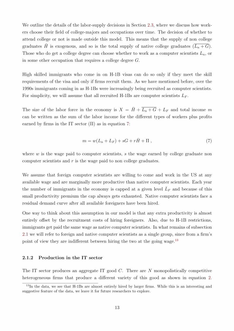
The size of the labor force in the economy is X = H + Ln +G + LF and total income m

can be written as the sum of the labor income for the different types of workers plus profits

earned by firms in the IT sector (Π) as in equation 7:

m = w(Ln + LF ) + sG+ rH + Π , (7)

where w is the wage paid to computer scientists, s the wage earned by college graduate non

computer scientists and r is the wage paid to non college graduates.

We assume that foreign computer scientists are willing to come and work in the US at any

available wage and are marginally more productive than native computer scientists. Each year

the number of immigrants in the economy is capped at a given level LF and because of this

small productivity premium the cap always gets exhausted. Native computer scientists face a

residual demand curve after all available foreigners have been hired.

One way to think about this assumption in our model is that any extra productivity is almost

entirely offset by the recruitment costs of hiring foreigners. Also, due to H-1B restrictions,

immigrants get paid the same wage as native computer scientists. In what remains of subsection

2.1 we will refer to foreign and native computer scientists as a single group, since from a firm’s

point of view they are indifferent between hiring the two at the going wage.13

2.1.2 Production in the IT sector

The IT sector produces an aggregate IT good C. There are N monopolistically competitive

heterogeneous firms that produce a different variety of this good as shown in equation 2.

13In the data, we see that H-1Bs are almost entirely hired by larger firms. While this is an interesting andsuggestive feature of the data, we leave it for future researchers to explore.

13

Following the framework introduced by Hopenhayn (1992) and Melitz (2003), each of these

firms will have a different level of productivity. Each firm j has a Cobb Douglas technology in

the labor aggregate and intermediate inputs from the other sector as in equation 8:

cj = φjLβc y

ψ1

cj x1−ψ1

cj , (8)

where ycj is the amount of intermediate goods from sector Y and xcj is the labor aggregate.

Firm technology, A(`j) = φjLβc , has an endogenous component Lβc and an exogenous component

φj which is a productivity draw that varies across firms. The term Lβc captures a technological

spillover in the IT sector which depends on the total number of computer scientists employed.

Since computer scientists are innovators, their innovations create spillovers that increase the

productivity of all firms in the sector, and this is captured by the β term.

The firm employs all three types of labor available in the economy in a nested Constant Elas-

ticity of Substitution (CES) structure.

xj =[αch

τ−1τ

j + (1− αc)qτ−1τ

j

] ττ−1

, (9)

where hj is the number of non college graduates and qj is the labor aggregate for college

graduates. Here τ is the elasticity of substitution between college graduates and non-college

graduates. Due to the nested nature of the CES function, we know that qj is:

qj =[(δ + ∆)`

λ−1λ

j + (1− δ −∆)gλ−1λ

j

] λλ−1

, (10)

where `j is the number of CS workers and gj the non-CS college graduates employed by firm

j. Here λ is the elasticity of substitution between the CS workers and non-CS college gradu-

ates.

In equation 8 it is clear that the IT sector firms have two drivers of technological change. The

exogenous component of technology φj, has been modeled similar to the setup in the trade

and the industrial-organization literature (Chaney (2008); Hopenhayn (1992); Melitz (2003)).

The endogenous component of technology, captured by β, depends on the total number of

computer scientists hired by the IT sector. These computer scientists innovate and create

new technologies, increasing overall firm productivity. Here, we modify the set-up used in

the literature on economic growth (Acemoglu (1998); Arrow (1962); Grossman and Helpman

(1991); Romer (1990)).14

14Since we do not model economic growth, there are some clear departures from this literature. While manypapers assume that the rate of change of technology depends on the quantity of a type of labor, we assumethe level of technology depends on labor. Furthermore, a lot of this literature models a separate R&D sectorthat sells patents for these technologies – whereas in our model technology is assumed to be non-excludable.

14

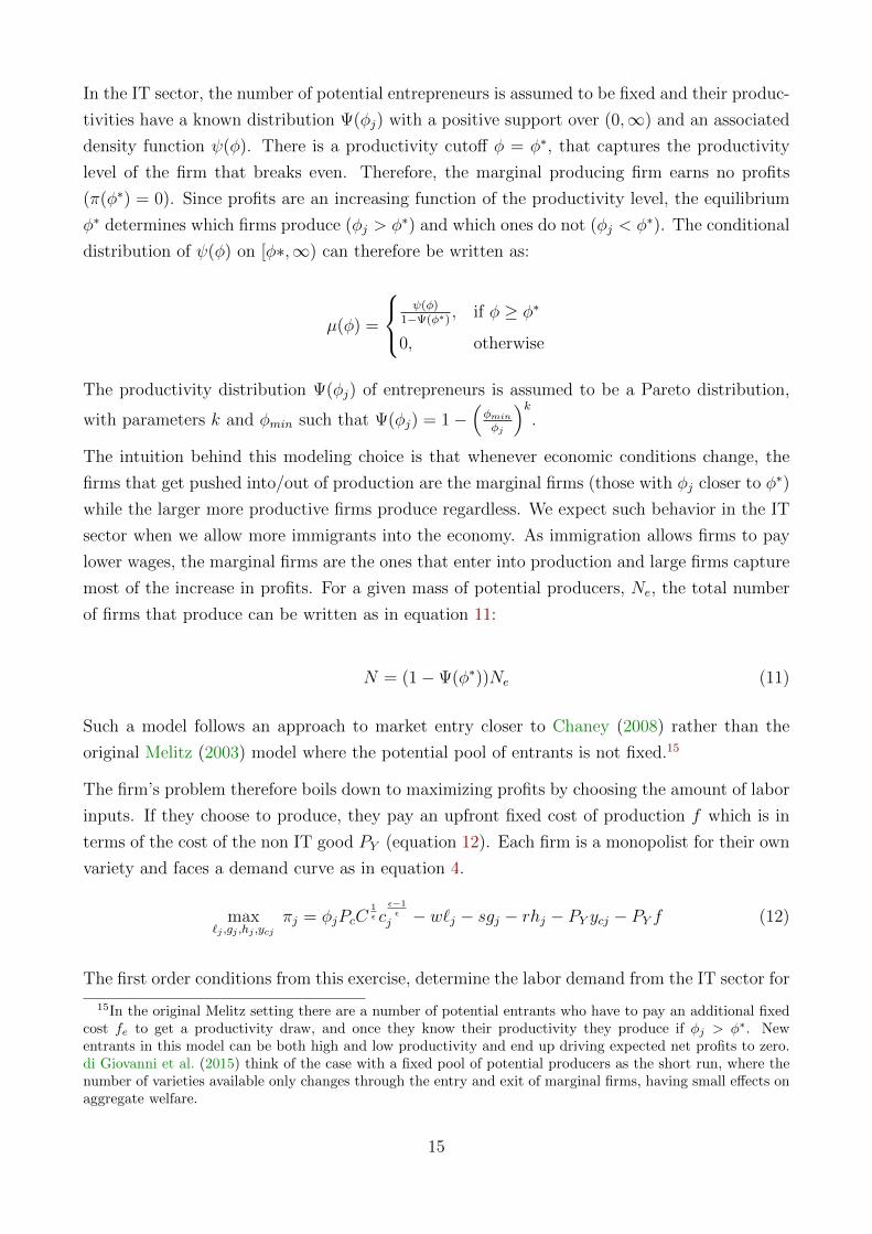
In the IT sector, the number of potential entrepreneurs is assumed to be fixed and their produc-

tivities have a known distribution Ψ(φj) with a positive support over (0,∞) and an associated

density function ψ(φ). There is a productivity cutoff φ = φ∗, that captures the productivity

level of the firm that breaks even. Therefore, the marginal producing firm earns no profits

(π(φ∗) = 0). Since profits are an increasing function of the productivity level, the equilibrium

φ∗ determines which firms produce (φj > φ∗) and which ones do not (φj < φ∗). The conditional

distribution of ψ(φ) on [φ∗,∞) can therefore be written as:

µ(φ) =

ψ(φ)

1−Ψ(φ∗), if φ ≥ φ∗

0, otherwise

The productivity distribution Ψ(φj) of entrepreneurs is assumed to be a Pareto distribution,

with parameters k and φmin such that Ψ(φj) = 1−(φminφj

)k.

The intuition behind this modeling choice is that whenever economic conditions change, the

firms that get pushed into/out of production are the marginal firms (those with φj closer to φ∗)

while the larger more productive firms produce regardless. We expect such behavior in the IT

sector when we allow more immigrants into the economy. As immigration allows firms to pay

lower wages, the marginal firms are the ones that enter into production and large firms capture

most of the increase in profits. For a given mass of potential producers, Ne, the total number

of firms that produce can be written as in equation 11:

N = (1−Ψ(φ∗))Ne (11)

Such a model follows an approach to market entry closer to Chaney (2008) rather than the

original Melitz (2003) model where the potential pool of entrants is not fixed.15

The firm’s problem therefore boils down to maximizing profits by choosing the amount of labor

inputs. If they choose to produce, they pay an upfront fixed cost of production f which is in

terms of the cost of the non IT good PY (equation 12). Each firm is a monopolist for their own

variety and faces a demand curve as in equation 4.

max`j ,gj ,hj ,ycj

πj = φjPcC1ε c

ε−1ε

j − w`j − sgj − rhj − PY ycj − PY f (12)

The first order conditions from this exercise, determine the labor demand from the IT sector for

15In the original Melitz setting there are a number of potential entrants who have to pay an additional fixedcost fe to get a productivity draw, and once they know their productivity they produce if φj > φ∗. Newentrants in this model can be both high and low productivity and end up driving expected net profits to zero.di Giovanni et al. (2015) think of the case with a fixed pool of potential producers as the short run, where thenumber of varieties available only changes through the entry and exit of marginal firms, having small effects onaggregate welfare.

15

each type of labor. Total labor hired by this sector is denoted by the subscript c, and aggregate

employment of each type of worker can be expressed as Lc, Gc and Hc.

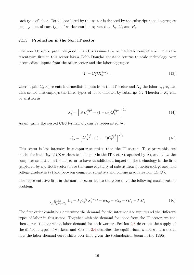
2.1.3 Production in the Non IT sector

The non IT sector produces good Y and is assumed to be perfectly competitive. The rep-

resentative firm in this sector has a Cobb Douglas constant returns to scale technology over

intermediate inputs from the other sector and the labor aggregate.

Y = Cψ2y X1−ψ2

y , (13)

where again Cy represents intermediate inputs from the IT sector and Xy the labor aggregate.

This sector also employs the three types of labor denoted by subscript Y . Therefore, Xy can

be written as:

Xy =[αyH

τ−1τ

y + (1− αy)Qτ−1τ

y

] ττ−1

(14)

Again, using the nested CES format, Qy can be represented by:

Qy =[δL

λ−1λ

y + (1− δ)Gλ−1λ

y

] λλ−1

(15)

This sector is less intensive in computer scientists than the IT sector. To capture this, we

model the intensity of CS workers to be higher in the IT sector (captured by ∆), and allow the

computer scientists in the IT sector to have an additional impact on the technology in the firm

(captured by β). Both sectors have the same elasticity of substitution between college and non

college graduates (τ) and between computer scientists and college graduates non CS (λ).

The representative firm in the non-IT sector has to therefore solve the following maximization

problem:

maxLy ,Gy ,Hy ,Cy

Πy = PyCψ2y X1−ψ2

y − wLy − sGy − rHy − PcCy (16)

The first order conditions determine the demand for the intermediate inputs and the different

types of labor in this sector. Together with the demand for labor from the IT sector, we can

then derive the aggregate labor demand for each worker. Section 2.3 describes the supply of

the different types of workers, and Section 2.4 describes the equilibrium, where we also detail

how the labor demand curve shifts over time given the technological boom in the 1990s.

16

2.2 Trade with the Rest of the World

The US economy trades both IT goods and the other good with the rest of the world (W).

IT firms export final goods to consumers in other countries, whereas US consumers import the

other good from the rest of the world.16

Consumers in the rest of the world (W) have the same utility function as US consumers:

UW (CW , YW ) =[γWC

σ−1σ

W + (1− γW )Yσ−1σ

W

] σσ−1

(17)

Since the US is the only producer of IT goods, foreign consumption is equivalent to US exports

of IT goods. Imports into the US from the rest of the world are represented by YIM . For

convenience we assume trade is balanced implying that the value of imports must equal the

value of exports:

PcCW = PyYIM (18)

Here we assume that the US is the only producer of IT. Even though Freeman (2006) stresses

how high-skill immigration may help the US maintain its comparative advantage in IT, we

may, expect that immigration policy affects IT production elsewhere in the world, especially

via the diffusion of knowledge. Khanna and Morales (2015) draw up a general equilibrium

model of both the US and India – the other major producer of IT – to study how the H1B

program affects production, human capital accumulation and labor market welfare for agents

in both countries. The possibility of migrating to the US induces students and workers in

other countries to accumulate CS-specific human capital, and return migrants help facilitate

the diffusion of technology. Over time, in the latter half of the 2000s, India becomes the major

exporter of IT, eroding the US’s comparative advantage. Khanna and Morales (2015) can be

thought of as a long-run extension of our current work, with consistent implications for the

period of study here – the 1990s.

2.3 Labor Supply of U.S. Computer Scientists

The firms’ decision problem determines not only the product market equilibrium but also the

demand curves for the different types of labor. To describe the workers’ decisions we develop a

dynamic model of labor supply that captures the choices made in deciding a field of study in

college, and occupational choices later in life. The model builds on previous work by Freeman

(1975, 1976); Ryoo and Rosen (2004) and closely follows the set-up of Bound et al. (2015).

16While we do not explicitly model outsourcing decisions, we do allow for the fact that imported goods in theother sector can be used as intermediate goods in production for the IT sector.

17

While Bound et al. (2015) was a partial equilibrium model that studied the decisions made

between CS and STEM occupations for a given labor demand elasticity, we extend it to a

general equilibrium framework which includes all types of labor and rigorously model the firm’s

decision to derive the labor demand curve that the workers face as well.

While we model the decisions to choose a field of study for US workers who attend college,

we do not explicitly model the decision to attend college in the first place. This is because we

assume that changes in wages for computer-science related occupations do not greatly affect the

college-going decision for students. The supply of workers who have only a high school degree

H is therefore assumed to be the same whether or not there were changes in the number of

foreign computer scientists in the labor market. Therefore the total supply of US workers with

a college degree (Ln +G) is also assumed to be fixed. However, we do model the decisions of

these college-educated workers as they make choices between majoring in CS degrees or other

degrees and then their occupation-choices in each year of their life till retirement.

In our model, there are three potential sources of CS workers. First, there are those who earn

computer science bachelor’s degrees from US institutions and join the workforce only after they

finish college. Second, there are college-educated US residents working in other occupations

who can switch into computer science, but must pay costs to switch occupations. Third, there

are foreigners who are being recruited on temporary work visas.

Given that most foreign workers that come on H-1Bs are computer scientists, we model CS

as the only profession that they get hired into. There are therefore two sources of non-CS

college-educated workers – those that graduate with any degree that is not computer-science

and those that switch from CS work to non-CS work by paying the switching cost.

We model US college graduates as maximizing their life-time utility by making two types of

decisions. When they are 20 years old, they choose their field of study in college which influences

their initial occupation at graduation. From ages 22 to 65, they choose between working as

a computer scientist or in another occupation. All individuals have rational, forward looking

behavior and make studying and working decisions based on the information available in each

period.

The labor demand curve derived from the firms’ decision problem discussed in the previous

sections, shifts out yearly due to productivity shocks. These shifts help identify the labor-

supply parameters and trace out the labor supply curve.

2.3.1 Field of Study Decision

In our model students choose their field of study when they are undergraduate juniors. Equation

19 captures this decision. At age 20, a student i draws idiosyncratic taste shocks for studying

computer science or another field: ηcsi and ηoi ,respectively. This student has expectations about

18

the prospects of starting a career in each occupation after graduation (age 22), which have

values V cs22 and V o

22 respectively. Given this information, an individual chooses between pursuing

computer science or a different choice of major at the undergraduate level.17

Worker utility is a linear function of their tastes and their career prospects in each sector

and they discount their future with an annual discount factor ρ. Additionally, there is an

attractiveness parameter θo for studying in a field that is not computer science, that all students

experience. This parameter may be negative if, on average, students prefer studying computer

science.

maxρ2EtV cs22 + ηcsi , ρ2EtV o

22 + θo + ηoi (19)

We assume that the individual taste parameters ηcsi and ηoi are independently and identically

distributed and for d = cs, o, can be defined as ηdi = σ0vdi , where σ0 is a scale parameter and

vdi is distributed as a standard Type I Extreme Value distribution. This assumption allows the

decisions of agents to be formulated in aggregate probabilities, and is therefore commonly used

in dynamic discrete choice models (Rust (1987), Kline (2008)).

Given these distributional assumptions, it follows that the probability (qcst ) that a student

graduates with a computer science degree can be written in logistic form:

qcst = [1 + exp(−(ρ2Et−2[V cs22 − V o

22]− θo)/σ0)]−1 (20)

One crucial parameter for how studying choices are sensitive to different career prospects is

the standard deviation of taste shocks. Small values of σ0 imply that small changes in career

prospects can produce big variations in the number of students graduating with a computer

science degree.

This set-up allows us to map the graduating probability described above to employment. Let

(Lat +Gat ) be the number of college graduates with age a in time period t, then the number of

graduates with a computer science degree in year t is represented by Rt = qcst (L22t +G22

t ).

2.3.2 Occupational Choice

The field of study decisions determine if an individual enters the labor market at age 22, as

either a computer scientist or in a different occupation. However, individuals can choose to

switch occupations between the ages of 22 and 65. At the start of each period, individuals use

17We are assuming that students decide their major after the end of their second year in school. Bound et al.(2015) experiment with a four-year time horizon and doing so made little qualitative difference.

19

the information at hand and choose their occupation in order to maximize the expected present

value of their lifetime utility.

Switching occupations, however, is costly for the worker, and these costs vary with age. This

is because workers have occupational-specific human capital that cannot easily be transferred

across occupations (Kambourov and Manovskii, 2009). The occupational switchings costs are

modeled as a quadratic function of a worker’s age, allowing for the fact that it becomes increas-

ingly harder to switch occupations as workers get older.18

Like in the college major decision, we assume that workers have linear utility from wages, taste

shocks and career prospects.19 The value functions of worker i at age a between 22 and 64 at

time t if she starts the period as a computer scientist or other occupation are therefore going

to be:

V cst,a = maxwt + ρEtV cs

t+1,a+1 + εcsit , st − ζ(a) + ρEtV ot+1,a+1 + εoit + θ1 (21)

V ot,a = maxwt − ζ(a) + ρEtV cs

t+1,a+1 + εcsit , st + ρEtV ot+1,a+1 + εoit + θ1 (22)

where ζ(a) = ζ0 + ζ1a + ζ2a2, is the monetary cost of switching occupations at age a, and θ1

is the taste attractiveness parameter for not working as a computer scientist, experienced by

all workers. Finally, all workers retire at age 65 and their retirement benefits do not depend

on their career choices. Therefore, at age 65 workers face the same decision problem without

consideration for the future.

As in the college-major decision problem, we will assume that taste shocks are independently

and identically distributed and for d = cs, o can be defined as εdit = σ1vdit where σ1 is a scale

parameter and vdi is distributed as a standard Type I Extreme Value distribution.

Defining qdDt,a as the probability that a worker at age a between 22 and 64 moves from occupation

d to occupation D, it follows from the distributional assumptions that the probability of work-

ers switching from computer-science to other occupations, and vice versa can be represented

as:

qo,cst,a = [1 + exp(−(wt − st − ζ(a)− θ1 + ρEt[V cst+1,a+1 − V o

t+1,a+1])/σ1)]−1 (23)

qcs,ot,a = [1 + exp(−(st − wt − ζ(a) + θ1 + ρEt[V ot+1,a+1 − V cs

t+1,a+1])/σ1)]−1 (24)

18While our model has no general human capital accumulation and wages do not vary with the age of aworker, the implications of the model would still hold if individuals expect similar wage growth profiles in eachoccupation.

19Wages must be totally consumed in that same year and workers cannot save or borrow.

20

Here we can see that the switching probabilities depend upon both the current wage differential

and expected future career prospects in each occupation. The standard deviation of the taste

shocks, the sector attractiveness parameter and the cost of switching occupations will affect

the sensitivity of occupational switching to changes in relative career prospects.

Since individuals are forward looking, the working decisions depend upon the equilibrium dis-

tribution of their career prospects. Under the extreme value errors assumption, we can use the

properties of the idiosyncratic taste shocks distribution to derive the expected values of career

prospects (Rust (1987)). The expected value function for an individual at age a between 22

and 64 working as a computer scientists or in another occupation are respectively:

EtV cst+1,a+1 = σ1Et[$+lnexp((wt+1+ρEt+1V

cst+2,a+2)/σ1)+exp((st+1−ζ(a)+θ1+ρEt+1V

ot+2,a+2)/σ1)]

(25)

EtV ot+1,a+1 = σ1Et[$+lnexp((st+1+θ1+ρEt+1V

ot+2,a+2)/σ1)+exp((wt+1−ζ(a)+ρEt+1V

cst+2,a+2)/σ1)]

(26)

where gamma $ ∼= 0.577 is the Euler’s constant and the expectations are taken with respect

to future taste shocks.

Given this set-up we can use the occupational-switching probabilities to derive the aggregate

employment in each sector. Since we allow workers at age 22 to also pay the switching costs

and get their first job in an occupation that is different from their field of study, the number of

computer scientists at age 22 is a function of the number of recent graduates with a computer

science degree and the occupational-switching probabilities:

L22nt = (1− qcs,ot,22)Rt + qo,cst,22 [(L22

nt +G22t )−Rt] (27)

G22t = (1− qo,cst,22)[(L22

nt +G22t )−Rt] + qcs,ot,22Rt (28)

where Rt is the number of recent graduates with a computer science degree, and (L22nt+G

22t )−Rt

is the number of college graduates with any other degree. Similarly, the supply of computer

scientists at age a from 23-65 is a function of past employment in each occupation and the

switching probabilities:

Lant = (1− qcs,ot,a )La−1n,t−1 + qo,cst,a [Ga−1

t−1 ] (29)

21

Gat = (1− qo,cst,a )Ga−1

t−1 + qcs,ot,a [La−1n,t−1] (30)

where Lant is the exogenous number of workers in computer science at age a in time period t,

and Gat is the number of workers at age a working in other occupations.

The aggregate domestic labor supply of computer scientists and other workers is the sum across

all ages:

Lnt =a=65∑a=22

Lant (31)

Gt =a=65∑a=22

Gat (32)

Here we can see that the labor supply in each occupation depends on past employment, new

college graduates and on wages through the occupational switching probabilities.

2.3.3 Labor Supply of Foreign Computer Scientists

We model high skilled foreign workers as only being hired as computer scientists, since during

the 1990s a majority of H-1Bs were hired into this occupation. By 2001, more than 21% of all

computer scientists were born abroad and immigrated after the age of 18 (March CPS). We

assume that high skilled foreigners have a perfectly elastic labor supply curve to the US, since

the wage that a computer scientist could obtain in countries like India or China, for instance,

is substantially lower than it is in the US (Clemens, 2013). This wage premium creates a large

queue of foreigners ready to take jobs in the US. There is, however, an institutionally imposed

cap on the total number of H-1Bs that restricts the number of foreign computer scientists each

year.

Institutional requirements also force firms to pay foreigners the prevailing US wage. We as-

sume that the additional costs of recruiting foreigners offsets the productivity advantage that

foreigners may have over their US counterparts. During the 1990s, a large fraction of the CS

workers coming from abroad were on H-1B visas. Given that this was a period when the H-1B

cap was usually binding, and given our assumption that foreign and domestic CS workers are

effectively identical, we treat the quantity of foreign CS coming to the US as exogenous.

22

2.4 Equilibrium

Equilibrium in each period can be defined as a set of prices and wages (Pct, PY t, wt, st, rt),

quantities of output and labor (C∗t , Y ∗t , C∗dt, C∗yt, C

∗Wt, Y

∗dt, Y

∗ct, Y

∗IMt, L

∗nt, L

∗Ft, G

∗t , H

∗t ), number

of firms (Nt) and the productivity cutoff (φ∗t ) such that:20

• Consumers in the US and the rest of the world, maximize utility by choosing Ct and Yt

taking prices as given, and choose their college major and occupations taking wages as

given

• Firms in both sectors maximize profits taking wages and aggregate prices as given

• In the IT sector, the firm with productivity φ∗t gets zero profits. All firms with φjt > φ∗t

produce while those with φjt < φ∗t do not.

• Output and labor markets clear as in equations 33 - 38

Total consumer expenditure equals labor income plus firm profits (equation 33):

PtcC∗dt + PytY

∗dt = m = wt(L

∗nt + L∗Ft) + stG

∗t + rtH

∗t + (Πt + PytfNt) (33)

Total quantity produced in the IT sector equals domestic consumer demand, intermediate

inputs in the other sector, and exports (equation 34):

Nεε−1

t

(∫ ∞φ∗t

cε−1ε

it µ(φ)dφ

) εε−1

= C∗t = C∗dt + C∗yt + C∗Wt (34)

Total quantity produced in the other sector, net of inputs, equals domestic consumer demand

and intermediate inputs in the other sector (equation 35):

C∗ψ2y X∗1−ψ2

y = Y ∗t = Y ∗dt + Y ∗Ct + fN∗t − Y ∗IMt (35)

Trade in goods is balanced:

P ∗ctC∗Wt = P ∗ytY

∗IMt (36)

Given that the supply of non college graduates is inelastic Ht, and the demand comes from

both sectors, their labor market clears as in equation 37:

Ht = H∗ct +H∗yt (37)

20Note that we’ve introduced a t subscript to each of the variables to denote that there is a different equilibriumfor each time period

23

Total labor supply for college graduates (CS and non CS) is fixed, such that total demand for

college graduates has to be equal to total supply in each period (equation 38):

Lnt +Gt + LF = L∗t +G∗t = L∗ct + L∗yt +G∗ct +G∗yt (38)

Native college graduates face the decision of whether to work as computer scientists or in some

other occupation that requires a college degree. This decision is no longer static, but has an

inter-temporal dimension which requires the definition of the dynamic equilibrium in the labor

market for college graduates. As in Bound et al. (2015), this equilibrium is characterized by

the system of equations (19 - 32) and a stochastic process Zt. In particular, equations 25

and 26 characterize the expectations of workers with respect to future career prospects and

equations 31 and 32 describe the dynamic labor supply of US computer scientists and other

college graduates respectively.

A unique equilibrium is pinned down each period by an aggregate labor demand curve for US

computer scientists relative to other college graduates that comes from the product market

model.

Even though this labor demand curve from the two sectors has no closed form solution we will

express it as in equation 39, a setup that will prove to be useful for the calculations in the

following sections.

LntGt

= Zt + Υ

(wtst

)(39)

where Υ(wtst

) is a baseline relative demand curve that depends on the relative wage. Zt is a

shifter that can be thought of as a combination of the productivity shocks from the IT boom,

that shifts out the relative demand for computer scientists every year and the cap of foreign

computer scientists LF that shifts in the relative demand curve every period. Zt is assumed to

follow a random walk process with high persistence such that:

Zt = 0.999Zt−1 + 0.001Z + ξt (40)

where Z is the steady state value of Zt and ξt is an i.i.d. shock.21

The equilibrium in the labor market can be expressed by a mapping from the state variables:

s = Rt,L22n,t−1, ..., L

64n,t−1, G

22t−1, ..., G

64t−1, Zt−1 and exogenous productivity shock ξt to the values

of Lnt, wt, Gt, st and Vt, the vector of career prospects at different occupations for different

21We assume workers consider both the technological progress from the IT boom as well as the increase inimmigrants to be a series of highly persistent shocks.

24

ages, that satisfies the system of equations 19 to 32 as well as each period’s relative demand

curve.

3 Calibration

We calibrate the parameters of our model in order to determine how welfare changes due to

immigration. We have a total of 25 parameters: σ, ε, γ, γW , ψ1. ψ2, β, αc, αy, τ , λ, δ, ∆, k,

φmin, Ne and f from the product market and σ0, σ1, θ0, θ1, ζ0, ζ1, ζ2 and ρ from the US college

graduates labor market. We focus on the period 1994-2001 that corresponds to the IT boom

and when the H-1B cap was mostly binding.

In order to calibrate the different parts of the model we follow a sequential approach. First,

we calibrate the parameters in the product market assuming total labor supply of Lt, Gt and

Ht are fixed (i.e. ignoring the choice of native workers between Lt and Gt). What makes this

possible in our model is that fact that adjustment costs imply that the stock of the different

types of labor are fixed in the very short run. This approach is akin to the approaches taken

by Freeman (1975, 1976) and Ryoo and Rosen (2004) in their modeling of adjustments on the

labor market for scientists.

In the next step we use the calibrated parameters to derive the aggregate labor demand curve

for computer scientists relative to other college graduates for every year. As a third step,

we use the predicted shifts in labor demand to calibrate the parameters of the labor supply

curve of different types of college graduates. Finally, we use the calibrated labor supply curve,

labor demand curve and product demand parameters to calculate welfare under the economy

where immigration is encouraged via the H-1B program and the counterfactual scenario where

immigration is restricted.

3.1 Product Market Calibration

We calibrate the parameters of the product market to match different features of the data

as explained in sections 3.1.1 - 3.1.5. The details of the data we use, including sources and

definitions of the different sectors and occupations can be found in Appendix A.1.

The model is calibrated separately for each year between 1994 and 2001. While some parameters

are assumed to be constant over time, others change in order to capture structural changes in

the economy. Particularly, the production function parameters (αct, αyt, δt, ∆t, ψ1t and ψ2t)

will be re-calibrated every year to capture the technological change that affects the two sectors

during this period. This can be thought of as describing the skill-biased technological change

over this period, since the share of labor cost that these sectors spend in computer scientists is

25

increasing over time. The utility parameters γt and γWt are also allowed to shift over time to

capture changes in local and foreign consumer preferences towards the IT sector. A summary

of all calibrated parameters in the product market can be found in Table 2.

3.1.1 Domestic utility function parameters

The three parameters in the consumer utility function are σ, ε and γt. σ is the elasticity of sub-

stitution between the composite IT good C and the good Y . We calibrate this parameter using

the ratio of first order conditions of goods Y and C from the consumer’s utility maximization

problem: γ1−γ

(CY

)− 1σ = Pc

PY.

This relationship can be reformulated as:

log

(C

Y

)= −σ log

(1− γγ

)− σ log

(PcPY

)(41)

We estimate σ using a regression of the relative quantity-index on the relative price-index. We

use data from the Bureau of Economic Analysis’ (BEA) industry-specific price and quantity

indices.22 The BEA data allows us to distinguish prices and quantities in the IT sector, and all

the other sectors in the economy. The coefficient of this regression is statistically indistinguish-

able from σ = 1. Given the plausibly exogenous technological change during the period which

drives down prices, we use this estimate as our main specification and proceed using a Cobb

Douglas utility specification. We also run a series of robustness checks running the results for

different values of σ that are summarized in Appendix A.2.

ε, the elasticity across IT varieties, is calibrated using the markup condition that comes from

the IT firms’ profit maximization condition (equation 42). We follow an approach similar to

Gaubert (2015) and match average value added to cost ratios for the IT sector. The data for

this is again taken from the BEA’s annual industry accounts that report value added as well as

costs like compensation to employees and taxes. For a marginal cost MC(ci), the price-markup

can be used to determine the value of ε:

pi =ε

ε− 1MC(ci) (42)

We calibrate ε = 3.26. Bernard et al. (2003) calculate a value of 3.8 for all US plants, whereas

Broda and Weinstein (2006) find a value of 2.2 for varieties of ‘automatic data processing

22The BEA price indices methodology can be found here http://www.bea.gov/national/pdf/chapter4.pdf andat http://www.bls.gov/opub/hom/pdf/homch17.pdf. The specific methodology for personal computers andperipheral equipment are detailed at http://www.bls.gov/cpi/cpifaccomp.htm, where they discuss adjusting forquality as well. While they do adjust for quality differences, we may still underestimate quality changes in IT(Gordon, 1990), which would affect our estimate of β. We do a rigorous sensitivity analysis for different valuesof β.

26

machines and units.’ Since our estimates lie within this region, we believe them to be reasonable.

We show that our results are robust to other reasonable values of this parameter in Appendix

A.2.

We calibrate the distribution parameter γt to match the share of expenditures in the IT good

(using equation 43). Again we use data from the BEA on industry specific GDP of IT as a

share of total GDP.23

PcC

m=

Pc

Pc +(

1−γγPc

)σ (43)

We calibrate γt conditional on the equilibrium prices, the share of consumption of the IT good

and the calibrated value of σ. For the Cobb Douglas specification we just use the share of

IT industry GDP to total domestic GDP. As already discussed, γt is time-varying in order to

capture potential changes in consumer preferences over time for the IT good relative to the rest

of the goods in the economy. Table 2 shows how γt steadily rises from 0.042 at the start of the

period to 0.052 by the year 2001.

3.1.2 Foreign utility function

Consumers from the rest of the world are assumed to have the same utility function as consumers

in the US. While we assume the elasticity of substitution σ is the same for both countries

(σ = 1), the distributional parameter γtW is selected to match the share of consumption of the

rest of the world for US IT products. We use the share of exports in IT to US GDP and the

relative size of the US economy to the rest of the world to pin down this parameter. Again,

we allow this parameter to change over time to capture potential changes in preferences for

consumers abroad.

3.1.3 Production Function Parameters

The elasticity of substitution between high school and college grads (τ) and between computer

scientists and other college graduates (λ) are assumed to be time invariant and equal across

sectors. To calibrate τ we follow several influential papers that provide estimates for this

parameter such as Katz and Murphy (1992), Card and Lemieux (2001) and Goldin and Katz

(2007) and set τ = 1.7 which is an average of their estimates.24 We present our results for a

23For all time varying parameters that are matched to shares observed in the data we run a regression of theraw share on a linear and quadratic time trend to recover the time invariant parameters. We then predict theshare using those coefficients and calibrate the parameters to match the predicted shares.

24Katz and Murphy (1992) find 1.41, Card and Lemieux (2001) find estimates between 2-2.5 and Goldin andKatz (2007) find 1.64. Strictly speaking, these numbers refer to the elasticity of substitution between college andnon college educated labor in the US economy, while our parameter is sector specific. The aggregate elasticity

27

range of values of λ (1, 2 and 4) which correspond to aggregate relative labor demand elasticities

of 1.02, 1.99 and 3.98. Ryoo and Rosen (2004) estimate aggregate relative demand elasticities

that lie between 1.2 and 2.2 for engineers which are included in the range of values we use.

To calibrate the value of β, the technological spillover from total CS in the IT sector, we look

at the relationship between the price decline in IT and the increase in total CS working in

the sector. We use the aggregate CS in IT equilibrium condition that gives us a relationship

between prices of IT and total labor in CS as in equation 44:

logPc = f(wt, st, rt)−1

εlogCt − ψ1

ε− 1

εlogPy +

(1− β(ε− 1))

εlogLc (44)

We run the regression of log(Pc) on a linear and quadratic time trend, the log of quantity of IT

good, the log price of the other good and the log of total computer scientists in IT. The time

trend aims to capture fluctuations in the wages of the different types of workers over time. The

calibrated value of β is 0.233. Effectively, this procedure attributes all of the TFP change to

the increase in computer scientists working for the IT sector while in reality there are several

other factors that also affect technical progress in IT. As a result, our estimates will tend to

over estimate the impact of computer scientists on technological change. Our estimate is quite

close to the Peri et al. (2014) estimates of changes in TFP attributable to the total number of

STEM workers. In Appendix A.2 we explore the sensitivity of our results to our estimate of

β.

The production function parameters αct, αyt, δt, ∆t, ψ1t and ψ2t are calibrated separately every

year to reflect the skill-biased technological change the two sectors face during the period.

This allows us to capture that increasingly, firms in both sectors spend a higher share of their

expenditures on college graduates.

The share of expenditures on non college graduates in both sectors are matched to the observed

share of labor income for each year in the March Current Population Survey (CPS). Here we

define the shares observed in the data as ϑt,C,H and ϑt,Y,H , such that:

ϑt,C,H =αctH

τ−1τ

ct

αctHτ−1τ

ct + (1− αct)Qτ−1τ

ct

(45)

Where Hct and Hct are the quantities observed in the CPS for each sector. We analogously

calibrate αyt using the shares observed in the data (ϑt,Y,H , Hyt and Qct)

In both sectors we have the parameter δt that is the distributional parameter associated with

computer scientists. We calibrate this parameter to match the relative wage of CS to other

involves both within and between sector components. However, our simulations suggest that setting τ = 1.7produces an aggregate elasticity indistinguishable from 1.7 to the first digit.

28

college grads(wtst

). The IT sector has a higher share of CS than the Other sector, so we

calibrate the parameter ∆ to match the share of total labor expenditure spent in CS by the IT

sector in a manner similar to our approach for calibrating αyt and αct.

In Table 2 we can see how skill-biased technological change in the economy changes these

parameters over time. δt steadily increases over this period as both sectors want to hire more

computer scientists. The values of αyt and αct steadily decrease for both sectors showing that

they spend more of their income on college graduates than on high school graduates. Parameters

associated with the intermediate inputs from another sector (ψ1t, ψ2t) are calibrated using the

share of intermediate inputs from other sectors relative to the GDP which we obtain from the

Bureau of Labor Statistics’ (BLS) input-output tables.

3.1.4 Entry into Production in the IT sector

There are four parameters related to the entry-decision and productivity distribution in the IT

sector. The number of firms in the sector depend on f , the fixed cost of production, and Ne,

the mass of potential producers. The Pareto distribution parameters k and φmin, determine the

productivity levels of these firms. All these parameters are assumed to be time-invariant.

We calibrate f to match the average firm size in the IT sector observed in the data for the

steady state year 1994. In order to do this we use information on the number of firms and

total employment in the IT sector from the Census’ Statistics of U.S. Businesses (SUSB).25 In

1994 we calibrate f to match the ratio of total employees and number of firms in the data for

the IT sector. The calibrated values for f are 1.24, 1.14 and 1.07 (for λ values of 1, 2 or 4

respectively). For the rest of the years we allow the number of firms Nt to adjust endogenously

as the profits from production change over time.

Ne is calibrated using information on establishment entry entry and exit.26 We look at the

total number of establishments over 500 employees in 2001 and calibrate the ratio of NtNe

= N94

N01.

Given that Nt in 1994 is used to calibrate f we get the rescaled Ne = 0.25.27

The Pareto distribution parameter k is set to match the standard deviation of logarithm of

US domestic plant revenues. Following Demidova (2008), we use the simulation reported by

Bernard et al. (2003) of 0.84. In our model the standard deviation of Ln(pici) is ε−1k

so given

our value of ε = 3.2 we get a value of k = 2.62. The scale parameter φmin is related to the

25This information comes from the 1992 Statistics of U.S. Businesses (SUSB). Since the information was onlyavailable for 1992 and 1997-2012, so we use the figures for 1992 as a proxy for 1994

26We get information on entry and exit of establishments in the IT sector by year from the Business DynamicsStatistics. Entry and exit was only available for establishments, not firms when looking at specific industries.

27Other papers such as Demidova (2008) and Melitz and Redding (2015) use the exit rate to calibrate param-eters related to fixed cost of production and entry but unlike us calibrate the slightly different Melitz (2003)model. The strategy we use is somewhat different as we have a fixed pool of potential entrants.

29

choice of units in which to measure productivity so we follow the convention in the literature

and normalize it to 1.

3.1.5 Total Quantity of Labor

To calibrate the product market parameters, we use the total quantities observed in the data

for each occupation type Lt, Gt and Ht as if they were exogenously given. We normalize the

US working population from the March CPS in 1994 to 100, and then allow for the population

in our model to grow at the same rate as the growth in the US population. The shares of each

type of worker are set equal to those observed in the data each year which allows us to know

the total number of college and non-college graduate workers, as can be seen in Table 3.

3.2 Deriving the Labor Demand Curve

Once we calibrate the product market parameters we are able to derive a labor demand curve

for computer scientists relative to other college graduates. Such a demand curve does not have

a closed form solution that comes directly from the model so we derive it by first changing the

relative values of LtGt

that we feed into the model and then calculating the predicted value of wtst

.

We run this exercise only for the steady-state year, 1994, and calculate wtst

for different values ofLtGt

that ranges between 0.04 and 0.07.28 We then fit a second order polynomial to get a closed

form solution of the relative labor demand curve.29

The elasticity of labor relative demand for computer scientists to other college graduates de-

pends crucially on the parameter λ. We derive the labor demand for our three values of λ

and get what we call the baseline labor demand curve as in equation 46, calculated using the

calibrated model for the steady state year 1994:30

LtGt

= Υ

(wtst, λ

)(46)

For the remaining years we allow the demand curve to shift for two reasons. First, to capture

the innovation taking place in the economy. This exogenous technological change is captured

by the time-varying parameters of the production functions. Second, the demand curve shifts

to capture the relative changes in the stock of college grads to non college grads which is

determined outside of the model.

28Relative total CS to other college graduates in the data is 0.0406 in 1994 and goes up to 0.0466 in 2001.We therefore capture more than the range of possible values in the data.

29The second order polynomial perfectly predicts the model with a R2 = 1. We experiment with higher orderpolynomials to fit the labor demand curve and our results do not change.

30The elasticity of the derived labor demand curve is very close to the value of λ, more specifically 1.015, 1.99and 3.98 for λ equal to 1, 2 and 4 respectively.

30

We can calculate the labor demand shifter Λt as in equation 47. This shifter applies to the

total demand of computer scientists relative to other college graduates, including both native

and foreign computer scientists.

Λt =LtGt

− Υ

(wtst

)(47)

As a last step, in order to use the variation in the demand curve to trace out the relative supply

curve for native computer scientists only, we subtract the relative number of foreign computer

scientists each year to derive to the total demand shifter Zt as presented in equation 39. As

a reminder, we treat the quantity of foreign CS workers coming to the US as exogenous since

the H-1B cap was binding throughout this period. Given that we assume foreign CS workers

are willing to work at any wage and are slightly more productive than natives, they get hired

first until they exhaust the H-1B cap while native workers face a residual labor demand curve.

The total shifter Zt = Λt − LtFGt

allows us to write the labor demand for native CS relative to

other college graduates as in equation 48:

LntGt

= Zt + Υ

(wtst

)(48)

In the steady state, Λ = 0 and Z = − L94,F

G94

3.3 Calibrating Labor Supply

On the labor supply side of the model, we have eight parameters that need to be calibrated

- σ0, θ0, σ1, θ1, ζ0, ζ1, ζ2, ρ. Of these, we pick the annual discount rate to be ρ = 0.9, and

calibrate the other parameters to match the data. In our model we assume the total quantities

of non college graduates Ht, native college graduates (Ln +G)t and foreign computer scientists

LtF are determined outside the model.

In the way we set-up the model, changes in lagged degree attainment, employment and wages

are driven by the exogenous technology shocks that shift out the demand curve for the different

types of labor over this decade. As the demand curve shifts, it traces out the labor supply

curve for workers. The technological developments that drive these shifts in the labor demand

are assumed to not affect the parameters of the workers’ labor supply decisions.

We use data on relative wages, employment, lagged degree attainment and age shares to cal-

ibrate the remaining seven parameters. The first three series compare computer scientists to

non-CS college graduate workers. For example, relative wages compare the wages for CS work-

ers with wages for non-CS college graduates. To do this, we use the March Current Population

31

Survey (CPS). Details of the sample used in the data and specific variable definitions can be

found in Appendix A.1.31

We simultaneously match wages, employment and the share of US computer science workers

that are young (between 22 and 40) in 1994 and 2001.32 We also match relative degrees in

computer science for 1994, 1997 and 2001. The series we use from the data are as follows:33

1. Ln,tGt

= US computer scientistsNon-CS college educated US workers

for t = 1994, 2001

2. wtst

= Median weekly wages for computer scientistsMedian weekly wages for non-CS college educated

for t = 1994, 2001

3.qcst+2

qot+2= US computer science college degrees awarded (lagged 2 years)

US non-CS college degrees awarded (lagged 2 years)for t = 1994, 1997, 2001

4. age22,40t = US computer scientists with age between 22 and 40

US CS22,40+US CS41,65 for t = 1994, 2001

To simultaneously find parameter values which solve the model under these data restrictions, we

use a Nelder-Mead simplex method. While the system uses all the data at the same time, there

is strong intuition behind the identification of each parameter. For example, the relative degree

attainment data should help identify the taste parameters for field of major decisions (σ0 and

θ0) as well as the fixed cost of switching occupations (ζ0), whereas the relative employment data

should help pin down the occupation specific tastes (σ1 and θ1). The age shares in computer

science employment help identify the occupation switching cost parameters that depend on age

(ζ1 and ζ2).

3.3.1 Labor Supply Calibration results

Figure 2 shows the data used and the model fit from this exercise. The figures report both the

path of the variables of interest predicted by the model, and the CPS data we use for these

series. We match two extreme years (1994 and 2001) for employment and wages and three

years (1994, 1997 and 2001) for lagged degree attainment, and the remaining years plotted are

an out of sample test of our method. The years in between (1995 to 2000) include years where

there were observed changes to immigration laws, and other potentially structural changes that

may make it difficult for the data to fit perfectly.

31We exclude imputed wages, and multiply top-coded values by 1.4. Bollinger and Hirsch (2007) showthat including imputations can lead to biased results. Whereas the top-coding adjustment is standard in theliterature (Lemieux, 2006). We smooth the raw data over three-year moving averages as follows: Xt,smooth =13 (Xt−1,raw +Xt,raw +Xt+1,raw)

32Given that in our labor supply model we impose all cohorts are the same size, we normalize the number ofcomputer scientists of a given age group dividing by the total number of college graduates in that age groupbefore calculating the age shares.

33We have an exactly identified system as we use nine data moments to recover ten parameters -σ0, θ0, σ1, θ1, ζ0, ζ1, ζ2 and two implied values of technology in the years we match the wage/employmentdata A94, A01

32

The employment series in Figure 2a and the wage series shown in Figure 2b fit well at the start

and end of the period, but it misses some years in between, particularly because it can’t match

the dip in wages that occur after 1994 and the simultaneous spike in employment in that same

period. Lastly, the lagged degree attainment series can be seen in Figure 2c, and matches the

data relatively well.

Table 4 presents the values of the calibrated parameters for the different values of λ. On

average, we can see that there is a mean taste for not working in CS occupations, which is

consistent with the wage differential seen across CS and non-CS work.

These calibrated parameters allow us to trace out the labor supply curve for computer-scientists

relative to non-CS college educated workers. In order to do this, we use the model set-up and

the parameters, and vary the relative wage to measure the response in relative quantities of

labor. This derives the relative supply curve which we then use in the labor market to find the

equilibrium wage.34

3.4 Endogenous Variables During the IT Boom

The calibration exercise so far helps us identify the parameters in the model that govern the

trends in the endogenous variables over time. We can study these trends to understand how

our model predicts what is happening at the time of the IT boom and the influx of foreign

computer scientists. Given the solution of the model in each period, we study how prices and

wages, employment by occupation and sector, and quantities produced change over time.

While US workers were more likely to work in CS occupations over time, the fraction of for-

eigners in CS work was increasing at a yet faster rate. Also consistent with the trends seen

in the data for this period, the wage for computer scientists increases faster than the wages in

other occupations. This IT boom overall leads to an increase in consumption of the IT good

and a fall in prices of the IT good which benefits consumers.

Figure 3a shows how the ratio of US computer-scientists to non-CS college graduates(LUSG

)evolves over this period according to our model for the different values of λ. During the time

of the boom this ratio increases from about 0.040 to 0.047 for λ = 2, as more and more US

workers shifted into CS work. At the same time, there was an increasing share of foreigners in

CS occupations – the ratio of foreign to US computer scientists(LForeignLUS

)more than doubled

from about 0.13 in 1994 to about 0.29 in 2001.

Our model predicts that over this period IT sector employment grew faster than employment

in the other sector, and most of this was driven by hiring in computer science occupations

(Figure 3b). The ratio of employment in IT to non-IT sectors over time(LC+GC+HCLY +GY +HY

)increases

34Our estimated relative labor-supply elasticities lie between 1.96 and 2.48.

33

over this period, highlighting the importance of the IT boom in employing more workers. At

the same time, with the influx of foreign computer scientists, the intensity of CS workers in

the IT sector eventually increases. This can be seen in the series that plots the ratio of CS to

non-CS workers in the IT sector(

LCGC+HC

)in Figure 3b. The overall growth in the IT sector

employment, therefore, was skewed towards CS employment.

While employment for CS workers, and the IT sector workers as a whole was increasing over

this period, we can also study how the relative wages for these types of workers change. Figure

3c plots the CS wage relative to non-CS college graduate workers wages(ws

)and relative to non-

college graduate workers wages(wr

). Consistent with the data, the model predicts that wages

for computer scientists increase at a faster rate than wages for the other types of workers.

The boom in the IT sector increased overall production and consumption for IT goods. Figure

3d shows how relative consumption(CY

)increases and relative prices

(PcPy

)fall over this period

as the supply of IT goods from firms increases. The reduction in the price of IT goods will

affect overall consumer utility as laid out by the model, and the following section will discuss

how we calculate utility for the different types of workers and the owners of firms.

4 Counterfactuals

In order to isolate the impacts of high-skilled immigration on the various endogenous variables

and on worker welfare, we conduct a counterfactual exercise. In the exercise we restrict the

stock of immigrants to be constant at the 1994 level, and subject the economy to the same

innovation shocks that were experienced during this period. Using the identified parameters,

we can then trace out what happens to all the endogenous variables over this period in a

situation where the stock of immigrants is fixed.

We use the notation ‘open’ to refer to the real scenario under the H-1B regime, and ‘closed’

to the counterfactual of restricted immigration. We can then define any endogenous variable

xs, under the two scenarios s = open, closed. For example, LUSopen is the number of US

computer scientists in the ‘real’ scenario under which high-skilled immigration is encouraged

via the H-1B program, and all CS workers earn a wage wopen. In contrast, LUSclosed and wclosed

are the employment of US computer scientists and wages for all computer scientists in the

counterfactual scenario where the stock of foreigners is restricted to its 1994 level.

4.1 Employment and College Degrees in CS

Figure 4a describes the restriction under the counterfactual exercise. It shows how, under the

real scenario where the economy is open to H-1B immigration, there is an increase in the stock

34

of foreign computer scientists, whereas under the counterfactual scenario where the economy is

‘closed,’ the stock of foreign computer scientists is restricted to the 1994 level.

How this restriction affects the stock of US computer scientists in our model can be seen in

Figures 4b-4c. Over this period there is an increase in the total number of computer scientists

when we allow for immigration, but the number of US computer scientists actually decreases

with respect to the closed economy every year as the number of immigrants increases. In 2001,

the number of US computer scientists was between 6.1%-10.8% lower under the open than in

the closed economy (Table 5). These numbers imply that for every 100 foreign CS workers that

enter the US, between 33 to 61 native CS workers are crowded out from computer science to

other college graduate occupations.

When the economy is open to immigration under the H-1B program, some US computer sci-

entists switch over to non-CS occupations, shifting out the supply of these workers. This can

be seen in Figure 4d. While over time there has been a rapid increase in the number of non-

CS college educated workers, this increase would have been lower if the number of foreign CS

workers were restricted. In fact, the growth rate between the open and closed economies plot-

ted in Figure 4d mirrors the decrease in Figure 4c as US workers switch from CS to non-CS

occupations.

Since students in our model choose their college major in their junior year, a change in the

wages for computer scientists will affect these choices. Under the open economy scenario the

fraction of CS degrees in 2001 would be between 1.3 - 2.6 percentage points lower than in the

closed economy as can be seen in Figure 4e.

4.2 Wages

Over the period of study, wages grew for computer science workers, but this growth would

have been higher if immigration was restricted (Figure 5b). An influx of foreign CS workers

depresses the CS wage, and shifts some US workers into non-CS occupations. At the end of

the decade, our model implies wages for CS workers would have been between 2.6%-5.1% lower

under the open economy (Table 5).

With an increase in the foreign CS workforce, college educated US CS workers shift into non-

CS occupations, and this tends to lower the non-CS wage. At the same time, however, as the

equilibrium amount of total CS workers increases, so does the marginal product of non-CS

college educated workers. This increases the demand for non-CS workers, and tends to increase

their wage making the net effect positive (Figure 5c). Overall, Table 5 shows an increase in

the non-CS wage due to immigration, of about 0.04%-0.28% in 2001. As expected both the

changes in CS wage and the non CS wage for college graduates are sensitive to what value of

λ we choose, but qualitatively our results do not change across specifications.

35

Since the labor supply of non-college graduates is assumed to be fixed and inelastic, only changes

in the demand for non-college graduates determine the difference in their wages under the real

and counterfactual scenarios. When the economy is open to immigration, the equilibrium

number of total college graduates employed increases due to immigration. This raises the

marginal product of non-college graduate labor, and shifts out the demand for non-college

graduate workers, raising the overall wage for non-college graduates (Figure 5d). Under the

open economy, wages for non-college graduates would have been between 0.43%-0.52% higher

by the end of this period (Table 5).35

4.3 Prices, Output and the Entry of Firms

While high-skilled immigration affected both employment and wages, it also affects overall

output and prices of the different goods produced in the economy. These changes will affect

overall consumer welfare, and also the profits accruing to firm owners.

Over the period of study, relative prices of IT goods were falling steadily, and some of this

fall can be attributed to the increase in CS employment due to immigration. Figure 6a and

Table 5 shows how under the open economy, prices would have been between 1.9%-2.4% lower

in 2001.

At the same time, the relative consumption of IT goods was increasing, and this increase would

have been lower without the growth in the foreign workforce (Figure 6b). Immigration also

raises the profits of firms who can now hire relatively cheaper labor, and this causes new firms

to enter the IT sector. Figure 6c shows how by allowing immigration, the number of IT firms

would be higher. At the end of this period, there would be between 0.50%-0.56% fewer IT firms

if immigration was restricted (Table 5).

5 Welfare

Using our estimated parameters and counterfactual exercises, we can measure the overall eco-

nomic impacts on the different agents in the economy due to the increase in the number of

foreign computer scientists. In order to compare losses and benefits and the distributional

consequences of immigration we look at the welfare of all types of workers and the owners of

firms.

35Since the non-college graduate workforce is a lot larger than the CS workforce the relative shift in wages isa lot lower compared to the CS wage.

36

5.1 Calculating Welfare

5.1.1 Calculating Worker Welfare

Given the structure of our CES utility function, we can calculate consumer welfare as a function

of the income of each type of agent. For a given income level mi, the indirect utility of the agent

is just the product of his income and the ideal price index. However, since the ideal price index is

the numeraire, indirect utility is just the income of each type of worker: Vi(mi) = mi. We then

compare the welfare of individuals under the two scenarios: (a) the real scenario, where high-

skill immigration is encouraged under the H-1B program, and (b) the counterfactual scenario

where the stock of immigrants is restricted to the 1994 level. For all welfare calculations we

will only be focusing on welfare changes for those individuals who are US born, ignoring the

changes in welfare for migrant computer scientists.

Workers are divided into four groups: those who are computer scientists and stay in CS oc-

cupations in the presence of immigration, those who are CS workers but switch to non-CS

work because of immigration, those who were non-CS college graduates even before there was

immigration and those who are non-college graduates. We then proceed to calculate welfare

changes in two different ways: percent utility changes and compensating variation.

Our model shows that when there is an influx of foreign computer scientists, the equilibrium

wage for CS workers falls and pushes some native college educated computer scientists into

non-CS work. As the equilibrium number of hired computer scientists increases, the marginal

product and hence the demand for other types of workers will also increase, tending to push up

their wages. The wage for non-college educated workers and college educated non CS workers

unambiguously rises for all specifications of λ.

For those that stay in their occupation groups under both real and counterfactual scenarios we

can calculate the percent utility changes by just looking at the percent change in the wage for

each group (e.g. the percent change in utility for the CS that stay in CS occupations under the

presence of immigration is just the percent change in w between the open and closed economy).

For CS that switch occupations to non-CS when we allow for immigration, we use information

from both the utility change for the CS that stay and the change for those that were always

non-CS college graduates.

By knowing the form of the indirect utility function, we can also calculate how much income

we must compensate different types of workers who lose from immigration. This compensating

variation (CV) depends on the indirect utility calculated at the original prices Pc and original

income levels mi, and compare it to a scenario with new prices and income (P ′c,m′i). A useful

feature of the compensating variation is that we can scale up the results using total labor income

in the US economy from the data, to measure how much workers should be compensated (in

USD) if immigration restrictions were imposed. Given that the the ideal price index is our

37

numeraire, we can write the compensating variation as CV = mi −m′i.

The number of computer scientists who stay in CS occupations even in the presence of im-

migration is Lopen. Their overall change in income in the presence of increased immigration

is therefore given by (wclosed − wopen)Lopen. When there is immigration, non college graduate

workers benefit from the rise in wages that is caused by the increase in their marginal product.

The increase in income for this group is therefore (ropen − rclosed)H.

Similarly, the number of non-CS college educated workers who were always in these other

occupations is given by Gclosed. Their overall change in income is given by (sclosed−sopen)Gclosed.

Given that we find the wages for college educated non-CS workers to be lower in the presence

of immigration, there is a loss in income to these workers due to immigration.

Lastly, for the group of workers who switch from CS to non-CS work in the presence of immigra-

tion, we must take into account their switching costs and change in utility because of different

tastes in each occupation. The marginal worker who switches, experiences a different loss in

utility than the infra-marginal worker. The overall change in terms of income equivalent for this

group of workers can be approximated by 12(Lclosed−Lopen) [(sclosed − sopen) + (wclosed − wopen)].36

5.1.2 Calculating Profits

In our model, firms in the perfectly competitive residual sector earn no profits. In the monopo-

listically competitive IT sector, however, only the marginal firm earns 0 profits. In the current

set-up we follow Chaney (2008), where there is an underlying mass of firms that already know

their entrepreneurial capabilities and choose whether to produce or not given their productivity.

There is therefore free-entry into the production decision, that drives the profit for the marginal

producing firm down to zero.

For the firms in the IT sector, the marginal producing firm has a productivity φ∗, and a profit

π(φ∗) = 0. Using the notation highlighted in Section 2.1, we know that the average profit for

producing firms can be represented by:∫ ∞φ∗

π(φ)µ(φ)dφ =

∫ ∞φ∗

PC1ε c

ε−1ε

j µ(φ)dφ−w∫ ∞φ∗

ljµ(φ)dφ− s∫ ∞φ∗

gjµ(φ)dφ− r∫ ∞φ∗

hjµ(φ)dφ− f

(49)

The total profits are then the average profits times the number of firms N = (1−Ψ(φ > φ∗))N e,

where N e is the number of total potential producers in the sector.

We can also calculate profits for different types of firms using the features of this distribution.

36The intuition for this expression is the following: a CS worker who switches, experiences a change in welfarethat equals the change in CS wage up to the relative wage that induces them to switch. From that point on,the additional change in welfare will equal the change in the wages of non-CS college grads. We assume thatfor minor changes in wages the demand curve can be approximated linearly.

38

For example, we know that the cutoff productivity will change across the regimes where there

is immigration and there isn’t. In the presence of immigration, firm profits will rise and allow

newer firms to enter on the margin.37 This then allows us to calculate the profits for the new

entrants and the incumbent firms separately. Let φ∗open and φ∗closed be the cutoff values of pro-

ductivity under each regime. The new firms that enter when there is immigration will have a

productivity φj ∈ [φ∗open, φ∗closed]. Whereas the incumbents have a productivity φj ∈ [φ∗closed,∞).

These cutoffs therefore change the limits of integration and the conditional distribution func-

tions.

The marginal distribution for the incumbents is determined by:

µclosed(φ) =

kφ−(k+1)

1−Ψ(φ∗closed), if φ ≥ φ∗

0, otherwise

With Ψ(φ∗closed) = 1−(

1φ∗closed

)kThe total profits to incumbents is then these average profits times the number of incumbents:

Nincumbent = (1 − Ψ(φclosed))Ne. The total profits for new entrants is simply the difference in

the profits for incumbents and the total profits for all firms in the open economy scenario.

Such an exercise can also be done to derive the profits for the firm in any percentile. For

example, the firm in the 90th percentile has a productivity φ90 = 10.1

1k . Since the number of

firms above the 90th percentile is simply N90 = 0.1Ne,we can derive the profits for these firms

in the scenario with and without immigration.

5.2 Welfare Changes Due to Immigration

The changes to the welfare of workers in this economy depends on the changes in income and

the prices due to immigration. Figures 7a, 7c and 7e show how much workers, under a regime

of restricted immigration, need to be compensated to maintain the same level of utility as they

had in the open economy. These numbers have been translated into 1999 USD. Overall worker

welfare is higher under immigration, and the amount of the compensating variation (CV) rises

steadily between 1994 and 2001. The CV for all workers in 2001 is between $8.2 and $10.9

billion depending on the value of λ.

This overall increase in utility due to immigration, however, hides a lot of distributional changes.

Figures 7a, 7c and 7e split up the workers into four groups - (1) those who stay in CS occupations

even after immigration, (2) those who switch from CS to non-CS, (3) college graduates who

were always non-CS, and (4) non-college graduates. As the figures show, US computer scientists

37Alternatively, in the Melitz (2003) framework of the model , firms will enter at any point of the distribution

39

are negatively affected by immigration, while other workers gain. The positive effect for college

graduates gets partly offset by the mobility of the college educated across occupations, where

CS switch to non-CS occupations depressing the wage. The losses for computer scientists and

the gains for non CS college grads get closer to zero when the ease of substitution between

CS and college non CS gets higher. On the other hand, the compensating variation for non

college grads increases when λ increases. Table 6 summarizes the utility percent changes from

allowing immigration and compensating variation for 2001, corroborating the idea that there

are significant distributional effects from increased immigration.

While workers, as a whole, benefit from more immigration, firms make higher profits too. In

Figures 7b, 7d and 7f the firms are split up into three different categories - (1) ‘all incumbents’

are only the firms that still produce when immigration is restricted. Amongst these incumbents,

the (2) ‘above 90th percentile’ firms are those that have a productivity level that is above the

90th percentile in the productivity distribution, and similarly (3) ‘75th to 90th’ percentile firms

have a productivity level that lies between the 75th and 90th percentiles. Profits for all firms

are increasing over this period and most of the profits are captured by the firms in the top ten

per-cent of the productivity distribution. While we believe there is considerable heterogeneity

in the profits firms receive as a result of the H-1B program it is important to note that the

distribution of profits in the model is determined by our assumption on the Pareto distribution

of firm productivities. In 2001, the aggregate profits in the IT sector were between $0.78 and

$0.89 billion (1999 USD), and between $0.59 to $0.68 billion went to the firms that had a

productivity level above the 90th percentile. Table 9 summarizes the changes in profits for the

different values of λ, overall profits increase between 0.61%-0.70% in 2001 when allowing for

immigration.

5.3 Alternative modeling specifications

We analyze how two particular features of the IT sector in our model affect our results. The

first is our assumption of monopolistic competition and the existence of different varieties

in IT products. This makes the IT sector smaller than the perfectly competitive optimal

size. An increase in the number of immigrants, and therefore workers, will expand this sector

and lead to welfare gains. At the same time, as more firms enter, the increase in varieties

benefit consumers as well. The second non-standard feature of our model is the presence

of technological spillovers driven by innovation by computer scientists. An increase in the CS

work force due to immigration leads to more innovation and has an additional impact on overall

production, lowering prices and increasing welfare for consumers.

In Table 7 we compare the monopolistically competitive model with a traditional perfectly

competitive set-up, and also shut-down the presence of technological spillovers to study how our

results change. In moving from a perfectly competitive to a monopolistically competitive model,

40

the welfare changes due to immigration are roughly similar. There is a slightly larger welfare

gain due to immigration in the monopolistically competitive model both in the absence or the

presence of technological spillovers. Shutting down the possibility of technological spillovers,

however, has a larger impact on the gains from immigration. In the absence of spillovers, β = 0,

the overall gains to worker utility is only between 0.02% and 0.03%, whereas the spillovers

β = 0.23 increase these gains to about 0.21%. How the results change with other values of β

is discussed in Appendix A.2. Therefore, while the monopolistic competition assumption does

not affect worker welfare much, the presence of technological spillovers does.

One advantage of the monopolistically competitive setup is that it allow us to get a measure of

how firm profits are affected by immigration. The profit numbers should be interpreted with

caution, however, since our framework implies that profits are simply a fixed proportion of total

revenues. Nonetheless, given that IT firms spend a substantial amount of funds in lobbying

Congress to raise the H-1B cap, it is reasonable to believe that firms stand to benefit from an

influx of high-skill immigrants.

Importantly, our model includes the labor supply decisions of college educated US workers.

This allows students and workers to move out of immigrant intensive fields and occupations

when there is an influx of high-skill workers from abroad. The negative effects on CS workers

is mitigated as US CS workers switch to non-CS jobs, and fewer students graduate with CS

degrees. However, since CS workers are also innovators, the economy as a whole no longer

benefits as much from technological improvements when US workers leave CS occupations. In

Table 8 we compare our baseline model that allows for labor supply decisions, to an inelastic

supply model where US students and workers are no longer allowed to change their decisions

in the face of high-skill immigration. Immigration has an even more of a negative impact on

US CS workers when we restrict adjustments on the labor supply side. Since workers can no

longer switch into non-CS occupations, the increase in labor supply from abroad depresses CS

wages and hurts CS workers the most. On the other hand, welfare in the economy as a whole

increases since there are more computer scientists and hence more innovators.

6 Discussion

Isolating the impacts of high-skill immigration is challenging in the absence of credible in-

struments that exogenously vary the share of foreign workers. Nonetheless, given the rapidly

increasing share of immigrants in the skilled labor force, it is an important issue to examine.

We develop a general equilibrium model of the US economy, calibrated using data from 1994

to 2001, to estimate how the increasing share of foreign high-skill workers affects the welfare

of different types of workers, firms and consumers. We do so by examining the welfare of US

natives under a counterfactual scenario where we restrict the fraction of immigrants to their

41

1994 levels.

While our conclusions depend on the specifics of our model, we believe them to be reasonable.

As long as the supply curve of US workers is not infinitely elastic, and we believe that evidence

indicates rather conclusively that it is not, the availability of high-skill foreign immigrants will

shift out the supply of high-skill workers in the US economy. However, as long as the demand

curve for high-skill workers is downward sloping, the influx of foreign high-skill workers will

both crowd out and lower the wages of US high-skill workers. As a result, output in the high-

skill intensive sector of the economy will rise, but will rise less than if the crowd out effects were

negligible. The fact that high-skill workers contribute to innovation tends to mute such crowd-

out effects, but our results suggest such effects are not nearly large enough to fully compensate

for the crowd-out.

Overall, our results suggest that high-skill foreign workers contribute to the well-being of the

typical US consumer, mainly through the assumption that these workers contribute to innova-

tion at the same rate as US high-skill workers. Indeed, under our calibrations, accounting for

foreign workers’ effect on innovation, the gains to consumers are an order of magnitude larger

than gains excluding this effect. At some level, this is hardly surprising. While simple models

of the impact of immigration on native welfare suggests the immigrant surplus is second order

(Borjas, 1999), if the immigrants shift out the production possibility frontier, their effect will

be first order.

In our model, immigration also raises profits in the IT sector. While the magnitude of these

gains depends on the markup in the IT sector, as long as there is a markup, which we consider

safe to assume, high-skill immigrant labor raises IT sector profits. It is then no surprise that Bill

Gates and other IT executives lobby in favor of increasing quotas for high-skill immigrants.

Although our results suggest that the introduction and expansion of the H-1B program in

the 1990s brought gains to both US consumers and IT sector entrepreneurs, we also found

indications of losses for US computer scientists and potential computer scientists. Recent work

(Peri and Sparber, 2009, 2011) has emphasized the importance of immigration affecting the

occupational choice of US natives. Our results tend to support the importance of this view.

Indeed, our estimates suggest that high-skill immigration has had a significant effect on the

choices made by US workers and students.

Researchers (e.g. Peri and Sparber, 2011) have emphasized that high-skill immigrants have

the potential for opening up opportunities for US workers – someone who might otherwise

have been an engineer or computer scientist now becomes a manager. We have no doubt that

this is true and, in a primitive way, we have built this into our model. The influx of skilled

immigrants induces some college graduates to leave CS and raises the productivity of non-CS

college graduates. Still, for many college graduates who entered or might have entered the CS

field, their options have been curtailed.

42

Our model is far too simple to allow for policy evaluations of alternatives to our current system

of high-skill immigration. However, we note that our model (and simple economic reasoning)

suggests that high-skill immigration does tend to crowd out US workers to some extent. We

suspect that allowing essentially unlimited immigration of high-skill workers by, for instance,

awarding green cards to all foreign students attending US colleges and universities would have

dramatic effects on the US labor market. Not all of these would be positive.

In the end we want to emphasize the limitations of our work. While our focus is on how the

influx of foreign workers affect the US, we recognize that US policy on high-skill immigration

has profound effects on both labor-sending countries and on other countries that produce in

the IT sector. Also, our analysis is constrained to the 1990s, whereas in the long run, US

immigration policy is likely to affect the position of the US in the world economy. We leave

exploration of these issues to future research.

43

References

Acemoglu, D. (1998). Why Do New Technologies Complement Skills? Directed Technical

Change and Wage Inequality. Quarterly Journal of Economics.

Arrow, K. J. (1962). The Economic Implications of Learning by Doing. The Review of Economic

Studies, Vol 29, Issue 3:155–173.

Bernard, A. B., Eaton, J., Jensen, J. B., and Kortum, S. (2003). Plants and Productivity in

International Trade. The American Economic Review, 93(4):1268–1290.

Bollinger, C. and Hirsch, B. (2007). How Well are Earnings Measured in the Current Popula-

tion Survey? Bias from Nonresponse and Proxy respondents. In North American Summer

Meetings of the Econometric Society, Duke University.

Borjas, G. (1999). The Economic Analysis of Immigration. Handbook of Labor Economics, Vol

3A, edited by Orley Ashenfelter and David Card, North-Holland.

Bound, J., Braga, B., Golden, J., and Khanna, G. (2015). Recruitment of Foreigners in the

Market for Computer Scientists in the US. Journal of Labor Economics.

Broda, C. and Weinstein, D. (2006). Globalization and the Gains From Variety. The Quarterly

Journal of Economics, 121(2):541–585.

Card, D. and Lemieux, T. (2001). Can Falling Supply Explain the Rising Return to College for

Younger Men? A Cohort-Based Analysis. The Quarterly Journal of Economics, 116(2):705–

746.

Chaney, T. (2008). Distorted Gravity: The Intensive and Extensive Margins of International

Trade. American Economic Review, 98(4):1707–1721.

Clemens, M. A. (2013). Why Do Programmers Earn More in Houston Than Hyderabad?

Evidence from Randomized Processing of US Visas. American Economic Review, Papers &

Proceedings, 103(3): 198-202.

Demidova, S. (2008). Productivity Improvements and Falling Trade Costs: Boon or Bane?

International Economic Review, 49(4):1437–1462.

di Giovanni, J., Levchenko, A., and Ortega, F. (2015). A Global View of Cross-Border Migra-

tion. Journal of the European Economic Association, 13(1):168–202.

Dixit, A. K. and Stiglitz, J. E. (1977). Monopolistic Competition and Optimum Product

Diversity. The American Economic Review, 67(3):297–308.

Doran, K., Gelber, A., and Isen, A. (2015). The Effect of High-Skilled Immigration Policy on

Firms: Evidence from H-1B Visa Lotteries. Working Paper. NBER Working Paper 20668.

44

Freeman, R. B. (1975). Supply and Salary Adjustments to the Changing Science Manpower

Market: Physics, 1948-1973. American Economic Review, 65(1):27–39.

Freeman, R. B. (1976). A Cobweb Model of the Supply and Starting Salary of New Engineers.

Industrial and Labor Relations Review, 29(2):pp. 236–248.

Freeman, R. B. (2006). Does Globalization of the Scientific/Engineering Workforce Threaten

U.S. Economic Leadership? Innovation Policy and the Economy, Volume 6, Adam B. Jaffe,

Josh Lerner, and Scott Stern.

Freeman, R. B. (2009). What Does Global Expansion of Higher Education Mean for the US?

Working Paper 14962, National Bureau of Economic Research.

Gaubert, C. (2015). Firm Sorting and Agglomeration. Working Paper.

Ghosh, A., Mayda, A. M., and Ortegae, F. (2014). The Impact of Skilled Foreign Workers

on Firms: an Investigation of Publicly Traded U.S. Firms. Working paper. IZA Discussion

Paper 8684.

Goldin, C. and Katz, L. F. (2007). Long-Run Changes in the Wage Structure: Narrowing,

Widening, Polarizing. Brookings Papers on Economic Activity, (2):135–65.

Gordon, R. (1990). The Measurement of Durable Goods Prices. National Bureau of Economic

Research, mimeo.

Grossman, G. M. and Helpman, E. (1991). Quality Ladders in the Theory of Growth. The

Review of Economic Studies.

Grossman, G. M. and Rossi-Hansberg, E. (2008). Trading Tasks: A Simple Theory of Off-

shoring. American Economic Review, 98(5):1978–1997.

Hopenhayn, H. A. (1992). Entry, Exit, and firm Dynamics in Long Run Equilibrium. Econo-

metrica.

Hunt, J. and Gauthier-Loiselle, M. (2010). How Much Does Immigration Boost Innovation?

American Economic Journal: Macroeconomics, 2(2):31–56.

Jorgenson, D. W., Ho, M. S., and Samuels, J. D. (2015). Education, Participiation and the

Revival of US Economic Growth. Paper for Conference on Research in Income and Wealth:

Education, Skills and Technical Change. Implications for Future US GDP Growth.

Kambourov, G. and Manovskii, I. (2009). Occupational Specificity Of Human Capital. Inter-

national Economic Review, 50(1):63–115.

Katz, L. F. and Murphy, K. M. (1992). Changes in Relative Wages, 1963-1987: Supply and

Demand Factors. The Quarterly Journal of Economics, 107(1):35–78.

45

Kerr, W. R. and Lincoln, W. F. (2010). The Supply Side of Innovation: H-1B Visa Reforms

and U.S. Ethnic Invention. Journal of Labor Economics, 28(3):473508.

Khanna, G. and Morales, N. (2015). The IT Boom and Other Unintended Consequences of

Chasing the American Dream. Mimeo.

Kirkegaard, J. (2005). Outsourcing and Skill Imports: Foreign High-Skilled Workers on H-

1B and L-1 Visas in the United States. Working Paper no. 05-15, Peterson Institute for

International Economics,Washington, DC.

Kline, P. (2008). Understanding Sectoral Labor Market Dynamics: An Equilibrium Analysis of

the Oil and Gas Field Services Industry. Cowles Foundation Discussion Papers 1645, Cowles

Foundation for Research in Economics, Yale University.

Krugman, P. (1979). A Model of Innovation, Technology Transfer, and the World Distribution

of Income. Journal of Political Economy, Vol. 87, No. 2:253–266.

Lemieux, T. (2006). Increasing Residual Wage Inequality: Composition Effects, Noisy Data,

or Rising Demand for Skill? The American Economic Review, 96:461–498.

Liu, R. and Trefler, D. (2008). Much Ado About Nothing: American Jobs and the Rise of

Service Outsourcing to China and India. NBER WP No. 14061, June.

Matloff, N. (2003). On the Need for Reform of the H-1B Non-Immigrant Work Visa in

Computer-Related Occupations. University of Michigan Journal of Law Reform, 36, no.

4:815–914.

Melitz, M. (2003). The Impact of Trade on Intra-Industry Reallocations and Aggregate Industry

Productivity. Econometrica, 71:1695–1725.

Melitz, M. and Ottaviano, G. (2008). Market Size, Trade, and Productivity. Review of Eco-

nomic Studies, 75:295–316.

Melitz, M. and Redding, S. (2015). New Trade Models, New Welfare Implications. American

Economic Review. Forthcoming.

Mithas, S. and Lucas, H. C. (2010). Are Foreign IT Workers Cheaper? U.S. Visa Policies and

Compensation of Information Technology Professionals. Management Science, 56(5):745–

765.

Mukhopadhyay, S. and Oxborrow, D. (2012). The Value of an Employment-Based Green Card.

Demography, 49:219–237.

Nathan, M. (2013). The Wider Economic Impacts of High-Skilled Migrants: A Survey of the

Literature. IZA Working Papers, Discussion Paper No. 7653.

46

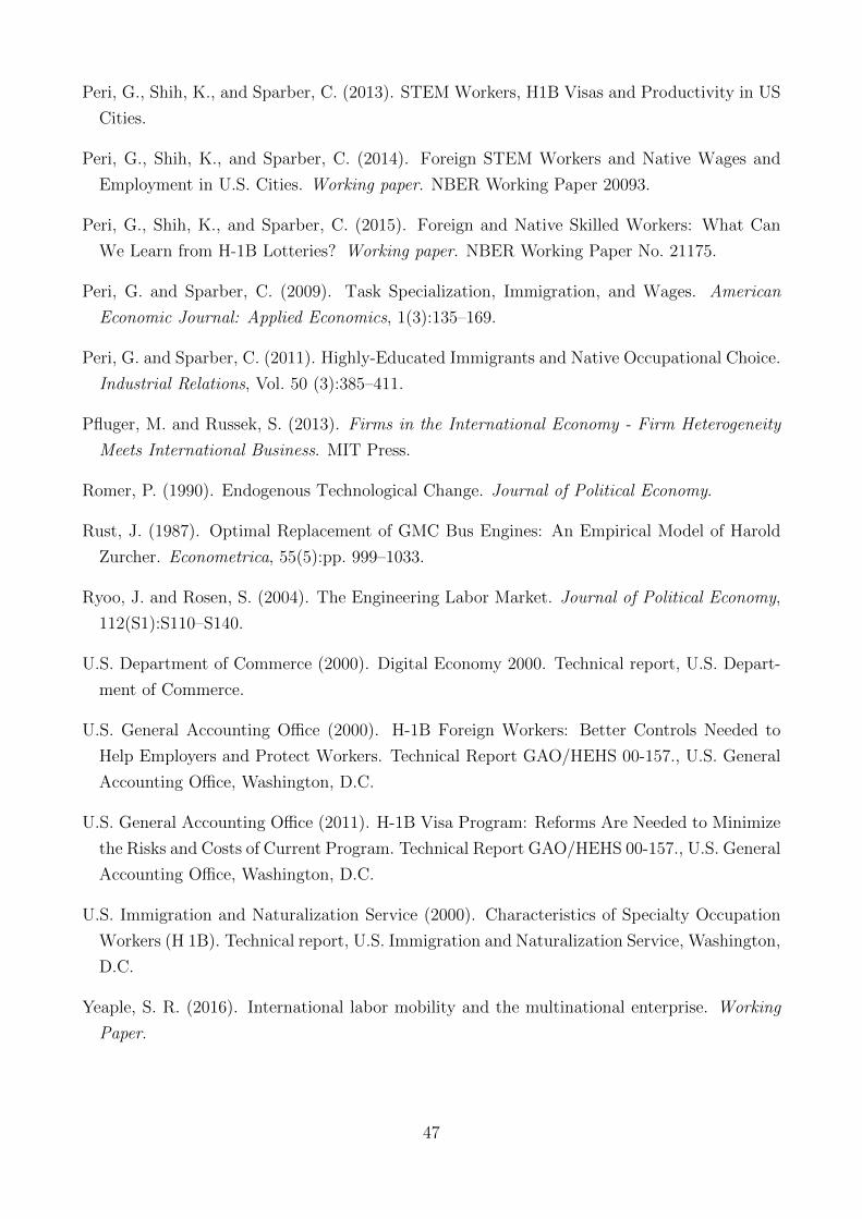
Peri, G., Shih, K., and Sparber, C. (2013). STEM Workers, H1B Visas and Productivity in US

Cities.

Peri, G., Shih, K., and Sparber, C. (2014). Foreign STEM Workers and Native Wages and

Employment in U.S. Cities. Working paper. NBER Working Paper 20093.

Peri, G., Shih, K., and Sparber, C. (2015). Foreign and Native Skilled Workers: What Can

We Learn from H-1B Lotteries? Working paper. NBER Working Paper No. 21175.

Peri, G. and Sparber, C. (2009). Task Specialization, Immigration, and Wages. American

Economic Journal: Applied Economics, 1(3):135–169.

Peri, G. and Sparber, C. (2011). Highly-Educated Immigrants and Native Occupational Choice.

Industrial Relations, Vol. 50 (3):385–411.

Pfluger, M. and Russek, S. (2013). Firms in the International Economy - Firm Heterogeneity

Meets International Business. MIT Press.

Romer, P. (1990). Endogenous Technological Change. Journal of Political Economy.

Rust, J. (1987). Optimal Replacement of GMC Bus Engines: An Empirical Model of Harold

Zurcher. Econometrica, 55(5):pp. 999–1033.

Ryoo, J. and Rosen, S. (2004). The Engineering Labor Market. Journal of Political Economy,

112(S1):S110–S140.

U.S. Department of Commerce (2000). Digital Economy 2000. Technical report, U.S. Depart-

ment of Commerce.

U.S. General Accounting Office (2000). H-1B Foreign Workers: Better Controls Needed to

Help Employers and Protect Workers. Technical Report GAO/HEHS 00-157., U.S. General

Accounting Office, Washington, D.C.

U.S. General Accounting Office (2011). H-1B Visa Program: Reforms Are Needed to Minimize

the Risks and Costs of Current Program. Technical Report GAO/HEHS 00-157., U.S. General

Accounting Office, Washington, D.C.

U.S. Immigration and Naturalization Service (2000). Characteristics of Specialty Occupation

Workers (H 1B). Technical report, U.S. Immigration and Naturalization Service, Washington,

D.C.

Yeaple, S. R. (2016). International labor mobility and the multinational enterprise. Working

Paper.

47

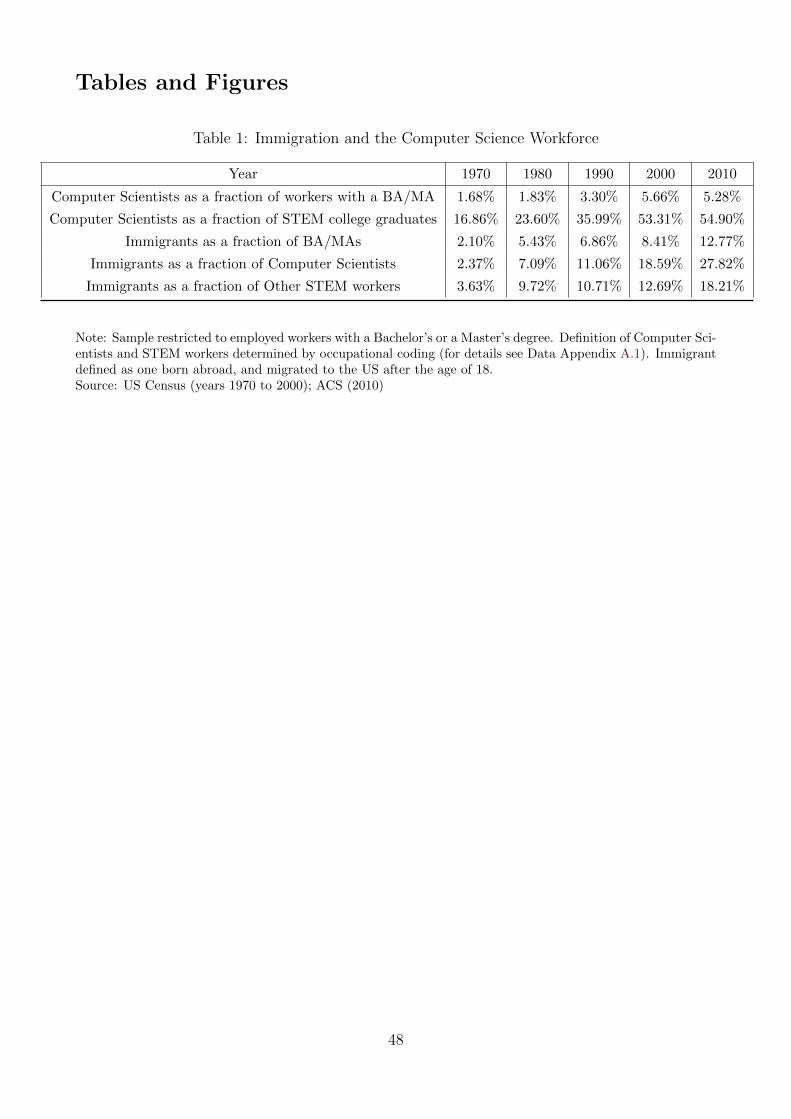
Tables and Figures

Table 1: Immigration and the Computer Science Workforce

Year 1970 1980 1990 2000 2010

Computer Scientists as a fraction of workers with a BA/MA 1.68% 1.83% 3.30% 5.66% 5.28%

Computer Scientists as a fraction of STEM college graduates 16.86% 23.60% 35.99% 53.31% 54.90%

Immigrants as a fraction of BA/MAs 2.10% 5.43% 6.86% 8.41% 12.77%

Immigrants as a fraction of Computer Scientists 2.37% 7.09% 11.06% 18.59% 27.82%

Immigrants as a fraction of Other STEM workers 3.63% 9.72% 10.71% 12.69% 18.21%

Note: Sample restricted to employed workers with a Bachelor’s or a Master’s degree. Definition of Computer Sci-entists and STEM workers determined by occupational coding (for details see Data Appendix A.1). Immigrantdefined as one born abroad, and migrated to the US after the age of 18.Source: US Census (years 1970 to 2000); ACS (2010)

48

Table 2: Calibrated Parameters from the Product Market

Time-Invariant Parameters

σ 1.00 k 2.62

ε 3.20 Ne 0.25

τ 1.70 f 1.07-1.24

β 0.23 φmin 1

Time-Varying Parameters

1994 1995 1996 1997 1998 1999 2000 2001

γ 0.042 0.046 0.050 0.052 0.054 0.055 0.055 0.054

γW 0.014 0.015 0.015 0.016 0.014 0.015 0.016 0.013

ψ1 0.522 0.524 0.525 0.524 0.523 0.521 0.517 0.513

ψ2 0.055 0.054 0.054 0.053 0.053 0.052 0.052 0.051

αc 0.438 0.432 0.427 0.419 0.410 0.401 0.395 0.390

αy 0.502 0.494 0.486 0.479 0.473 0.468 0.465 0.463

λ = 1 0.053 0.055 0.059 0.063 0.067 0.069 0.073 0.072

δ λ = 2 0.224 0.227 0.233 0.240 0.248 0.253 0.262 0.260

λ = 4 0.395 0.398 0.401 0.405 0.414 0.420 0.430 0.428

λ = 1 0.217 0.215 0.215 0.218 0.225 0.237 0.249 0.270

∆ λ = 2 0.174 0.168 0.153 0.147 0.146 0.157 0.158 0.175

λ = 4 0.073 0.066 0.048 0.039 0.036 0.046 0.042 0.057

σ: Elasticity of substitution between C and Y ; ε: elasticity of substitution

across IT varieties; τ : the elasticity of substitution between college and non

college graduates; β: the technological spillover of computer scientists in IT;

f : fixed cost of production; Ne: mass of potential producers; k and φmin:

distribution and scale parameters from the Pareto distribution.

γ: Distributional parameter of domestic CES utility; γW : Distributional pa-

rameter of foreign CES utility; ψ1, ψ2: Production function parameters for

Intermediate inputs in IT and the Other Sector respectively; αc, αy: Distribu-

tional parameter for non college grads in the IT and Other sector production

function; δ: Distributional parameter for computer scientists in both sectors;

∆: distributional parameter for computer scientists in IT. λ: Elasticity of

substitution between CS and non-CS college grads.

49

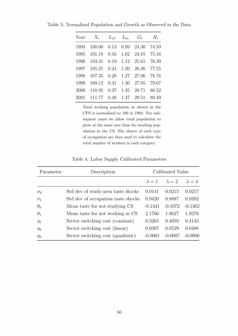
Table 3: Normalized Population and Growth as Observed in the Data

Year Xt LtF Ltn Gt Ht

1994 100.00 0.13 0.99 24.30 74.59

1995 101.18 0.16 1.02 24.85 75.16

1996 103.31 0.19 1.12 25.61 76.39

1997 105.25 0.24 1.20 26.26 77.55

1998 107.35 0.26 1.27 27.06 78.76

1999 109.12 0.31 1.30 27.85 79.67

2000 110.95 0.37 1.35 28.71 80.52

2001 111.77 0.40 1.37 29.51 80.49

Total working population as shown in the

CPS is normalized to 100 in 1994. For sub-

sequent years we allow total population to

grow at the same rate than the working pop-

ulation in the US. The shares of each type

of occupation are then used to calculate the

total number of workers in each category.

Table 4: Labor Supply Calibrated Parameters

Parameter Description Calibrated Value

λ = 1 λ = 2 λ = 4

σ0 Std dev of study-area taste shocks 0.0141 0.0215 0.0217

σ1 Std dev of occupation taste shocks 0.9420 0.8887 0.9282

θ0 Mean taste for not studying CS -0.1341 -0.1072 -0.1362

θ1 Mean taste for not working in CS 2.1766 1.8627 1.9278

η1 Sector switching cost (constant) 0.3265 0.4059 0.4145

η2 Sector switching cost (linear) 0.0307 0.0529 0.0488

η3 Sector switching cost (quadratic) -0.0001 -0.0007 -0.0006

50

Table 5: Percent Changes when Allowing Immigration - 2001

λ = 1 λ = 2 λ = 4

Relative Price -1.86% -1.85% -2.42%

Relative Quantity 1.89% 1.89% 2.48%

Number of Firms 0.50% 0.51% 0.56%

Wage Computer Scientists -5.13% -3.47% -2.57%

Wage College Graduates non CS 0.28% 0.10% 0.04%

Wage Non College Graduates 0.43% 0.44% 0.52%

Total Employment in CS 6.39% 8.00% 11.47%

US Computer Scientists -10.81% -9.32% -6.12%

College Graduates non CS 0.57% 0.48% 0.30%

Percent changes are calculated using the endogenous variables

from the closed and open economy. For each year we consider

the situation of going from a closed to an open economy (al-

lowing immigration), that is (XopenXclosed

− 1)× 100. Results shown

for different values of λ and only look at year 2001.

Table 6: Percent change in Utility when allowing for Immigration and Compensating Variation

Percent Change in UtilityCompensating Variation

(million USD)

λ = 1 λ = 2 λ = 4 λ = 1 λ = 2 λ = 4

All US workers 0.20% 0.21% 0.27% 8204 8290 10904

College Graduates - All -0.12% -0.16% -0.14% -1955 -2453 -2110

Computer Scientists that stay -5.13% -3.47% -2.57% -5951 -3752 -2631

Computer Scientists that switch -2.48% -1.71% -1.27% -348 -189 -85

College Graduates non CS that stay 0.28% 0.10% 0.04% 4344 1488 606

Non College Graduates 0.43% 0.44% 0.52% 10159 10743 13014

We compare utility changes when going from a closed to an open economy so percent changes are

calculated for each year and subgroup as: (VopenVclosed

− 1)× 100, where V is indirect utility for that

specific group. Compensating Variation figures are expressed in million USD.

51

Table 7: Percent change in Utility - perfect competition vs. monopolistic competition in theIT sector

Perfectly competitive Monopolistic competition

β = 0 β = 0.23 β = 0 β = 0.23

All US workers 0.02% 0.20% 0.03% 0.21%

College Graduates - All -0.34% -0.16% -0.34% -0.16%

Computer Scientists that stay -3.76% -3.58% -3.64% -3.47%

Computer Scientists that switch -1.90% -1.76% -1.85% -1.71%

College Graduates non CS that stay -0.08% 0.10% -0.08% 0.10%

Non College Graduates 0.25% 0.43% 0.26% 0.44%

We compare utility changes when going from a closed to an open economy so percent changes

are calculated for each year and subgroup as: (VopenVclosed

− 1)× 100, where V is indirect utility

for that specific group. In the perfectly competitive cases we assume that the IT sector is

no longer under monopolistic competition. The β = 0 refers to the case where there is no

spillover effect in the IT sector while the β = 0.23 refers to the spillover case. In all cases

λ = 2.

52

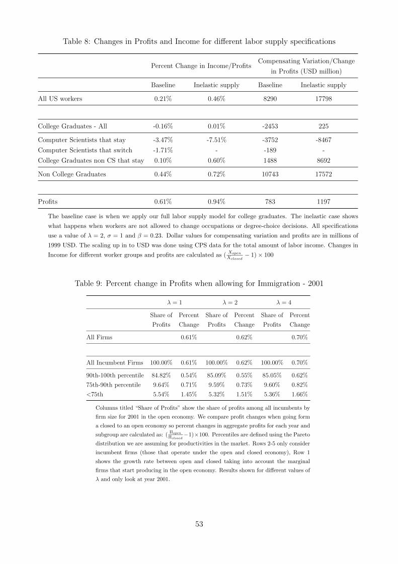
Table 8: Changes in Profits and Income for different labor supply specifications

Percent Change in Income/ProfitsCompensating Variation/Change

in Profits (USD million)

Baseline Inelastic supply Baseline Inelastic supply

All US workers 0.21% 0.46% 8290 17798

College Graduates - All -0.16% 0.01% -2453 225

Computer Scientists that stay -3.47% -7.51% -3752 -8467

Computer Scientists that switch -1.71% - -189 -

College Graduates non CS that stay 0.10% 0.60% 1488 8692

Non College Graduates 0.44% 0.72% 10743 17572

Profits 0.61% 0.94% 783 1197

The baseline case is when we apply our full labor supply model for college graduates. The inelastic case shows

what happens when workers are not allowed to change occupations or degree-choice decisions. All specifications

use a value of λ = 2, σ = 1 and β = 0.23. Dollar values for compensating variation and profits are in millions of

1999 USD. The scaling up in to USD was done using CPS data for the total amount of labor income. Changes in

Income for different worker groups and profits are calculated as (XopenXclosed

− 1)× 100

Table 9: Percent change in Profits when allowing for Immigration - 2001

λ = 1 λ = 2 λ = 4

Share of

Profits

Percent

Change

Share of

Profits

Percent

Change

Share of

Profits

Percent

Change

All Firms 0.61% 0.62% 0.70%

All Incumbent Firms 100.00% 0.61% 100.00% 0.62% 100.00% 0.70%

90th-100th percentile 84.82% 0.54% 85.09% 0.55% 85.05% 0.62%

75th-90th percentile 9.64% 0.71% 9.59% 0.73% 9.60% 0.82%

<75th 5.54% 1.45% 5.32% 1.51% 5.36% 1.66%

Columns titled “Share of Profits” show the share of profits among all incumbents by

firm size for 2001 in the open economy. We compare profit changes when going form

a closed to an open economy so percent changes in aggregate profits for each year and

subgroup are calculated as: (ΠopenΠclosed

−1)×100. Percentiles are defined using the Pareto

distribution we are assuming for productivities in the market. Rows 2-5 only consider

incumbent firms (those that operate under the open and closed economy), Row 1

shows the growth rate between open and closed taking into account the marginal

firms that start producing in the open economy. Results shown for different values of

λ and only look at year 2001.

53

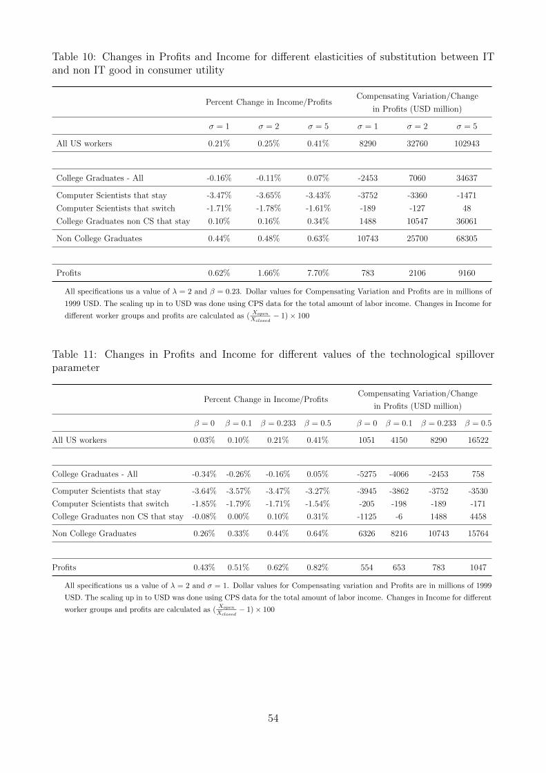
Table 10: Changes in Profits and Income for different elasticities of substitution between ITand non IT good in consumer utility

Percent Change in Income/ProfitsCompensating Variation/Change

in Profits (USD million)

σ = 1 σ = 2 σ = 5 σ = 1 σ = 2 σ = 5

All US workers 0.21% 0.25% 0.41% 8290 32760 102943

College Graduates - All -0.16% -0.11% 0.07% -2453 7060 34637

Computer Scientists that stay -3.47% -3.65% -3.43% -3752 -3360 -1471

Computer Scientists that switch -1.71% -1.78% -1.61% -189 -127 48

College Graduates non CS that stay 0.10% 0.16% 0.34% 1488 10547 36061

Non College Graduates 0.44% 0.48% 0.63% 10743 25700 68305

Profits 0.62% 1.66% 7.70% 783 2106 9160

All specifications us a value of λ = 2 and β = 0.23. Dollar values for Compensating Variation and Profits are in millions of

1999 USD. The scaling up in to USD was done using CPS data for the total amount of labor income. Changes in Income for

different worker groups and profits are calculated as (XopenXclosed

− 1)× 100

Table 11: Changes in Profits and Income for different values of the technological spilloverparameter

Percent Change in Income/ProfitsCompensating Variation/Change

in Profits (USD million)

β = 0 β = 0.1 β = 0.233 β = 0.5 β = 0 β = 0.1 β = 0.233 β = 0.5

All US workers 0.03% 0.10% 0.21% 0.41% 1051 4150 8290 16522

College Graduates - All -0.34% -0.26% -0.16% 0.05% -5275 -4066 -2453 758

Computer Scientists that stay -3.64% -3.57% -3.47% -3.27% -3945 -3862 -3752 -3530

Computer Scientists that switch -1.85% -1.79% -1.71% -1.54% -205 -198 -189 -171

College Graduates non CS that stay -0.08% 0.00% 0.10% 0.31% -1125 -6 1488 4458

Non College Graduates 0.26% 0.33% 0.44% 0.64% 6326 8216 10743 15764

Profits 0.43% 0.51% 0.62% 0.82% 554 653 783 1047

All specifications us a value of λ = 2 and σ = 1. Dollar values for Compensating variation and Profits are in millions of 1999

USD. The scaling up in to USD was done using CPS data for the total amount of labor income. Changes in Income for different

worker groups and profits are calculated as (XopenXclosed

− 1)× 100

54

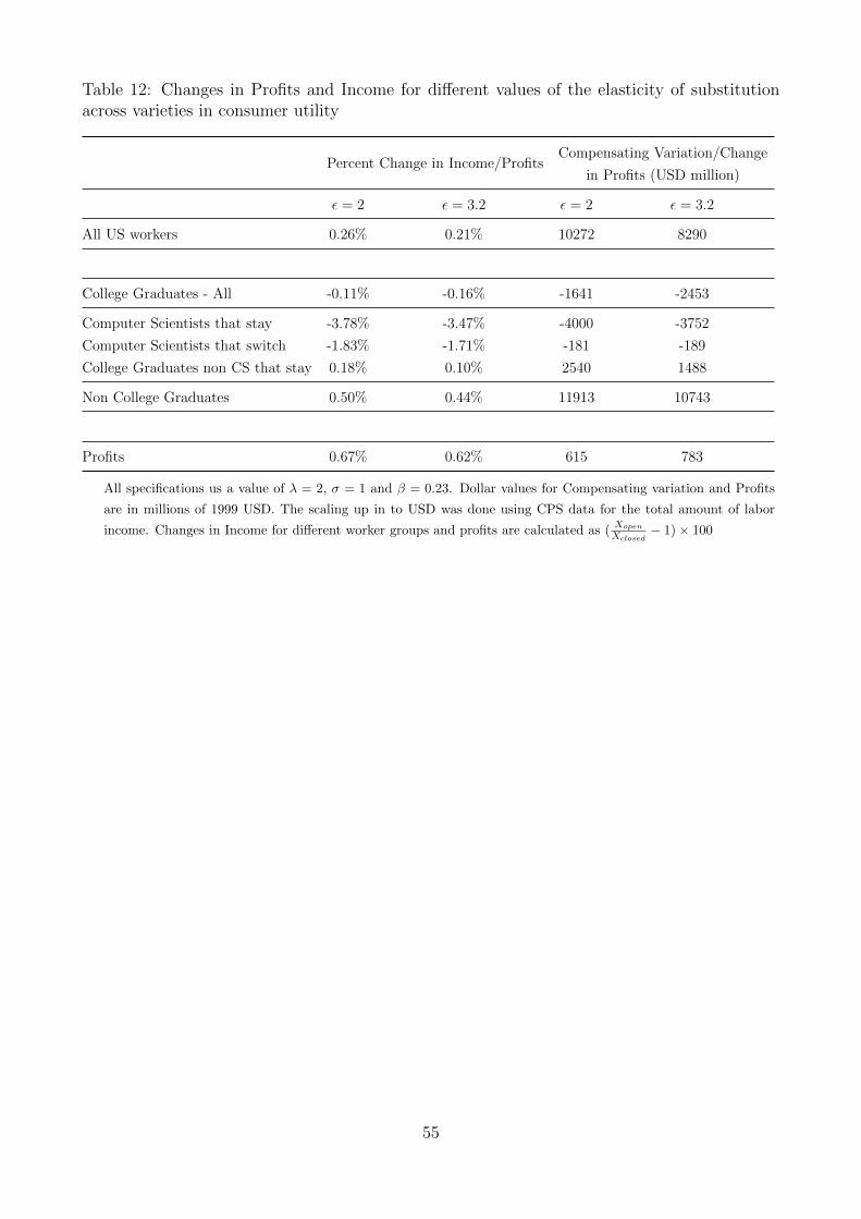
Table 12: Changes in Profits and Income for different values of the elasticity of substitutionacross varieties in consumer utility

Percent Change in Income/ProfitsCompensating Variation/Change

in Profits (USD million)

ε = 2 ε = 3.2 ε = 2 ε = 3.2

All US workers 0.26% 0.21% 10272 8290

College Graduates - All -0.11% -0.16% -1641 -2453

Computer Scientists that stay -3.78% -3.47% -4000 -3752

Computer Scientists that switch -1.83% -1.71% -181 -189

College Graduates non CS that stay 0.18% 0.10% 2540 1488

Non College Graduates 0.50% 0.44% 11913 10743

Profits 0.67% 0.62% 615 783

All specifications us a value of λ = 2, σ = 1 and β = 0.23. Dollar values for Compensating variation and Profits

are in millions of 1999 USD. The scaling up in to USD was done using CPS data for the total amount of labor

income. Changes in Income for different worker groups and profits are calculated as (XopenXclosed

− 1)× 100

55

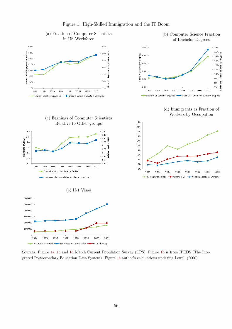
Figure 1: High-Skilled Immigration and the IT Boom

(a) Fraction of Computer Scientistsin US Workforce

(b) Computer Science Fractionof Bachelor Degrees

(c) Earnings of Computer ScientistsRelative to Other groups

(d) Immigrants as Fraction ofWorkers by Occupation

(e) H-1 Visas

Sources: Figure 1a, 1c and 1d March Current Population Survey (CPS). Figure 1b is from IPEDS (The Inte-

grated Postsecondary Education Data System). Figure 1e author’s calculations updating Lowell (2000).

56

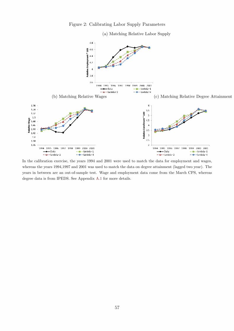
Figure 2: Calibrating Labor Supply Parameters

(a) Matching Relative Labor Supply

(b) Matching Relative Wages (c) Matching Relative Degree Attainment

In the calibration exercise, the years 1994 and 2001 were used to match the data for employment and wages,

whereas the years 1994,1997 and 2001 was used to match the data on degree attainment (lagged two year). The

years in between are an out-of-sample test. Wage and employment data come from the March CPS, whereas

degree data is from IPEDS. See Appendix A.1 for more details.

57

Figure 3: Endogenous Variables Over Time

(a) Ratio of Foreign to US Computer Scientistsand US CS to US College Graduates

(b) Computer Science Laborand Total Labor in IT

(c) Relative wages for CS workers(d) Relative Price and Quantity

of the IT Good

Model predictions for ratio of endogenous variables over time:

(a) Foreign CS workers to US CS workers(LForeignLUS

), and for US CS workers to all US College Graduate

workers(

LUSLUS+G

),

(b) Computer science labor to non-CS labor in the IT sector(

LcGc+Hc

)and the total labor in IT relative to

total labor in the other sector(Lc+Gc+HcLy+Gy+Hy

)(c) Computer science wage relative to non-CS college graduate wage

(ws

)and the computer science wage

relative to non-college graduate wage(wr

)(d) Relative prices for the IT good

(PcPy

)and relative consumption

(CY

).

58

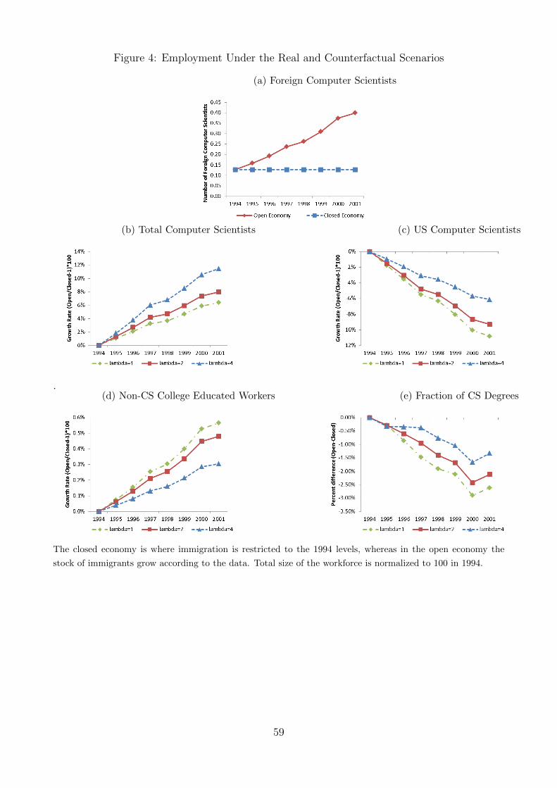
Figure 4: Employment Under the Real and Counterfactual Scenarios

(a) Foreign Computer Scientists

(b) Total Computer Scientists (c) US Computer Scientists

.(d) Non-CS College Educated Workers (e) Fraction of CS Degrees

The closed economy is where immigration is restricted to the 1994 levels, whereas in the open economy the

stock of immigrants grow according to the data. Total size of the workforce is normalized to 100 in 1994.

59

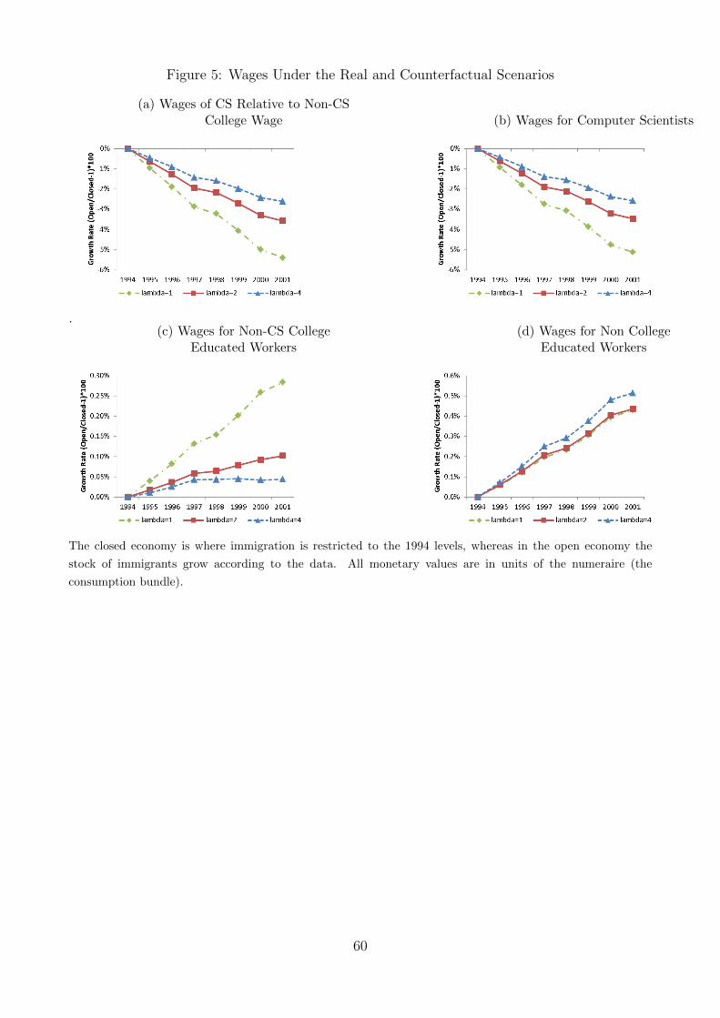
Figure 5: Wages Under the Real and Counterfactual Scenarios

(a) Wages of CS Relative to Non-CSCollege Wage (b) Wages for Computer Scientists

.(c) Wages for Non-CS College

Educated Workers(d) Wages for Non College

Educated Workers

The closed economy is where immigration is restricted to the 1994 levels, whereas in the open economy the

stock of immigrants grow according to the data. All monetary values are in units of the numeraire (the

consumption bundle).

60

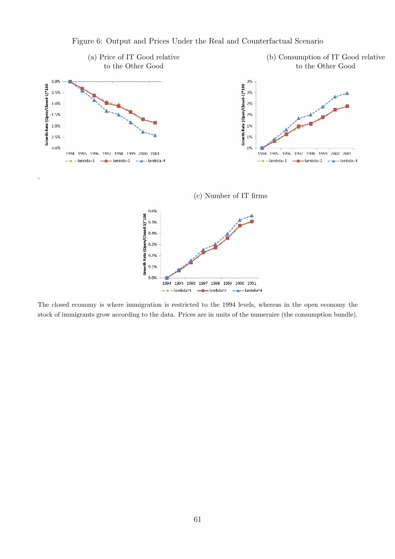
Figure 6: Output and Prices Under the Real and Counterfactual Scenario

(a) Price of IT Good relativeto the Other Good

(b) Consumption of IT Good relativeto the Other Good

.

(c) Number of IT firms

The closed economy is where immigration is restricted to the 1994 levels, whereas in the open economy the

stock of immigrants grow according to the data. Prices are in units of the numeraire (the consumption bundle).

61

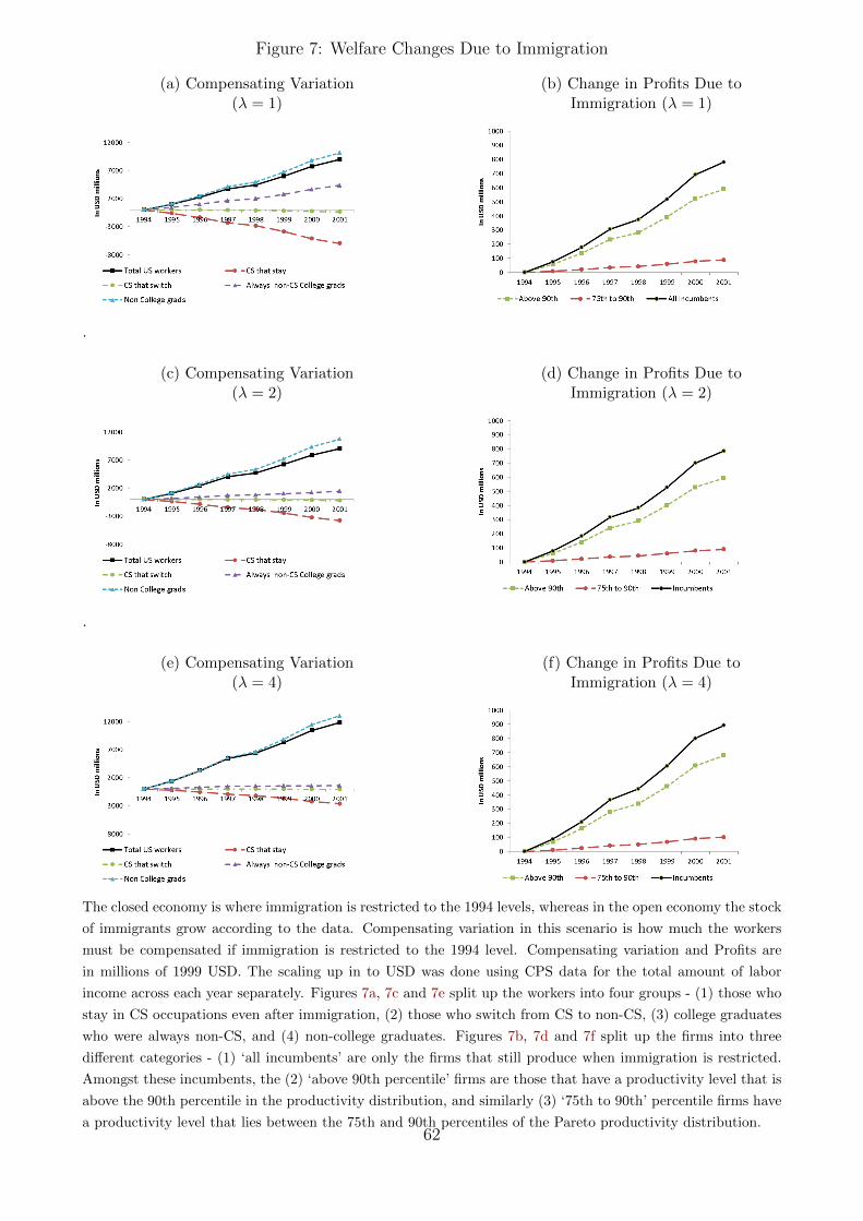
Figure 7: Welfare Changes Due to Immigration

(a) Compensating Variation(λ = 1)

(b) Change in Profits Due toImmigration (λ = 1)

.

(c) Compensating Variation(λ = 2)

(d) Change in Profits Due toImmigration (λ = 2)

.

(e) Compensating Variation(λ = 4)

(f) Change in Profits Due toImmigration (λ = 4)

The closed economy is where immigration is restricted to the 1994 levels, whereas in the open economy the stock

of immigrants grow according to the data. Compensating variation in this scenario is how much the workers

must be compensated if immigration is restricted to the 1994 level. Compensating variation and Profits are

in millions of 1999 USD. The scaling up in to USD was done using CPS data for the total amount of labor

income across each year separately. Figures 7a, 7c and 7e split up the workers into four groups - (1) those who

stay in CS occupations even after immigration, (2) those who switch from CS to non-CS, (3) college graduates

who were always non-CS, and (4) non-college graduates. Figures 7b, 7d and 7f split up the firms into three

different categories - (1) ‘all incumbents’ are only the firms that still produce when immigration is restricted.

Amongst these incumbents, the (2) ‘above 90th percentile’ firms are those that have a productivity level that is

above the 90th percentile in the productivity distribution, and similarly (3) ‘75th to 90th’ percentile firms have

a productivity level that lies between the 75th and 90th percentiles of the Pareto productivity distribution.62

A Appendix

A.1 Details of the Data Used

This study draws on a variety of datasets. Our descriptive statistics in Table 1 rely on the

IPUMS Census from 1970 to 2000. We restrict the sample to employed workers. We use the

IPUMS suggested occupation crosswalk and define computer scientists as computer systems

analysts, computer scientists and computer software developers with at least a BA degree. We

define foreigners as either naturalized citizens or non-citizens who immigrated after the age of

18. For early Census years the year of immigration is only available in ranges. In order to

construct a precise year of immigration value for workers in those samples we choose to select

a random value within the year range for each individual.

Data on earnings, domestic employment and foreign employment used in the calibration proce-

dure and in the descriptive figures come from the March CPS, obtained from the IPUMS and

NBER websites. The sample consists of employed persons with at least a BA degree. A person

is defined as foreign if he/she was born outside the United States and immigrated after the age

of 18. Earnings are deflated to 1999 dollars, and top-coded values are multiplied by 1.4.

In our analysis we drop imputed earnings. In order to identify these imputed values, we use a

methodology similar to (Bollinger and Hirsch (2007)). From the IPUMS database we use the

qinclongj and qincwage variables, and from the NBER database we use the FL665 flag to identify

imputations. The database also contains ten Census Bureau flags that identify a small fraction

(less than 1%) of earnings as allocated. Over the period under study around 26% of earnings

were allocated. This fraction of imputations varies over time - between 19.14% (in 1994) and

29.47% (in 2003). These numbers are consistent with (Bollinger and Hirsch (2007)) who find

that between 1998 and 2006, the non-response rate was about 20%. The small difference in our

numbers arises both from using a different sample (restricted to those with BA/MA degree)

and because non-response is not the only reason the CPS imputes earnings.

In order to define workers in Computer Science we use the occupational codes in the CPS

Outgoing Rotation Group (CPS-ORG) data set. The occupational coding in the CPS-ORG up

to 2002 uses the 1990 Census definition. We consider as Computer Scientists those under the

occupational titles of: “055 Electrical and electronic,” “064 Computer systems analysts and

scientists” and “229 Computer programmers”.

College degree attainment data is based on Integrated Post-secondary Education Data System

(IPEDS) Completions Survey. It consists of bachelor’s degrees awarded by the NSF popu-

lation of institutions. We consider enrollment in computer science and electrical engineer as

the number of degrees awarded in these fields lagged by 2 years. For 1994 and 1995, degree

attainment in electrical engineering was not available by native and foreign students but only

I

shown together with all engineering degrees. We input the data for these two years by looking

at the average growth in electrical engineering for 1996-2002.

In descriptive statistics, we compare the computer science workforce to STEM workers. STEM

occupations are defined as engineers, computer systems analysts and computer scientists, com-

puter software developers, operations and systems researchers and analysts, actuaries, statis-

ticians, mathematicians and mathematical scientists, physicists and astronomers, chemists,

atmospheric and space scientists, geologists, physical scientists n.e.c., agricultural and food sci-

entists, biological scientists, foresters and conservation scientists, and medical scientists.

We use data on the prices, quantities, costs and value added from the Bureau of Economic

Analysis (BEA) since this source allows us to look into data for specific industry groups. Data

on firm entry and exit comes from the Business Dynamic Statistics (BDS), and the 1992 Census’

Statistics of U.S. Businesses (SUSB). In these data sets we define the IT sector as the sub-sectors

of “Computer and electronic product manufacturing,” “Publishing industries, except Internet

(includes software),” “Data processing, Internet publishing, and other information services” and

“Computer systems design and related services” according to the NAICS 2002 classification.

The Non IT sector is defined as all other sectors in the economy.

A.2 Sensitivity Analysis

We check how sensitive our results are to variations in key parameters and specifications of the

model. So far we have presented all our results for three different values of λ. Despite slight

differences in the magnitudes of changes in income and profits, the results are qualitatively

similar across different values of this parameter. For simplicity we fix λ = 2 when doing our

sensitivity analysis on all the other parameters of the model.

First we look at how sensitive our results are to variations in the elasticity of substitution

between the IT good and the non IT good, represented by the parameter σ. As we see in Table

10, the more elastic the relative product demand curve, the larger the income increase for all

US workers is when we allow for immigration. This is consistent with economic intuition since

a higher value of σ implies that consumers are more willing to substitute consumption from

non-IT to IT goods. When we allow for immigration, the larger number of computer scientists

in the economy increases the size of the IT sector and consumers shift into consuming more

IT goods. Profits for IT firms rise and workers that are complements to CS workers are better

off for higher values of σ. Furthermore, since IT production drives technological change, as

and when more resources are devoted to IT for higher values of σ, the price of IT goods falls

increasing overall welfare. Overall our qualitative results are similar for different values of σ

with the only difference being that for high values of σ the population of all college graduates

is better off due to immigration.

II

We also vary the technological change parameter and check how sensitive our results are to

reasonable values of β. Our calibrated value of β is 0.233, and we re-do our results for values

of 0, 0.1 and 0.5. Table 11 shows how the compensating variation and profits change as we

vary β. Immigration is benefecial for higher values of β, for all types of US workers and firms

since a larger CS workforce increases the gains from technology. Firms directly benefit from

higher output, whereas consumers benefit from lower prices as the value of β rises. Overall,

however, our qualitative results are similar across the different β levels. The only qualitative

difference is that for the scenario where there is no technological progress (β = 0), the sub

population of college graduates non CS are worse off when there is immigration. This happens

because without the spillover of aggregate computer scientists, the positive effect they had for

being complements to CS gets smaller and is offset by the lower wages caused by CS switching

occupations.

Last, we vary the elasticity of substitution between varieties of the IT good ε across a reasonable

range. In Section 5.3 we discuss results for the baseline case where the goods are perfect

substitutes and all IT firms are similar. In Table 12 we see that as we lower the elasticity

of substitution ε to from a value of 3.2 to 2, the overall welfare gains from immigration are

enhanced. While close substitutes in the labor market are worse off for smaller values of ε,

complements are better off. The overall impacts, however, are similar both qualitatively and

quantitatively.

In other results, we test to see whether using a Melitz (2003) style model of entry significantly

affects our conclusions and found out that it does not. In our baseline model there is an

underlying fixed number of potential entrepreneurs that always know their level of productivity

φj, a set-up closer to Chaney (2008). An alternative set-up is one where firms do not initially

know their level of productivity φj, but must pay a fixed sunk cost fe to draw their level of

productivity from the known distribution. Firms wish to pay this cost as long as their expected

profits are positive. As more firms draw and produce, expected profits fall till they are zero.

Once a firm draws their productivity φj, they may choose to pay another fixed cost f and

produce if φj > φ∗. This setup is closer to the one described by Melitz (2003).38

We may expect these set-ups to have different implications for firm profits and overall welfare. In

our baseline model, an increase in immigration, tends to increase firm profits and the marginal

firms enter into producing goods. Since all firms already know their productivity level, the more

productive firms always produce. The new entrants are therefore firms that have a productivity

level in the immediate neighborhood of φ∗. The overall increase in productivity, therefore, is

small since the new entrants are firms that have relatively low productivity. Furthermore, the

increase in profits is almost entirely captured by the larger firms. In the alternative Melitz

(2003) framework, entry may happen at any part of the productivity distribution. When the

38To see a discussion about these two models in the context of immigration models, see di Giovanni et al.(2015).

III

expected profits rise because of immigration, new entrants may potentially draw very high

levels of productivity and enter at the extreme tails of the distribution. The overall increase

in productivity is higher which drives down the price of the IT good, and increases consumer

utility. Furthermore, the new entrants capture all the increase in profits whereas the profits

for the incumbents do not change. Compared to the baseline model, we find that the change

in welfare due to immigration is higher under the Melitz entry set-up both because of higher

aggregate profits and consumer utility. This is because the new firms that enter the industry

are not just the firms with marginal productivity, but could also be firms with very high

levels of productivity. These firms have higher profits, and drive down the output prices more.

Qualitatively, however, all our results stay the same across the two models.

IV