-f -

SEISMICITY, TECTONICS, AND SURFACE WAVE PROPAGATION

IN THE CENTRAL ANDES

by

GERARDO SUAREZ

Ingeniero Geofisico, Universidad Nacional Aut6noma de Mexico(1976)

SUBMITTED TO THE DEPARTMENT OFEARTH AND PLANETARY SCIENCES

IN PARTIAL FULFILLMENTOF THE REQUIREMENTSFOR THE DEGREE OF

DOCTOR OF PHILOSOPHY

at the

MASSACHUSETTS INSTITUTE OF TECHNOLOGY

December 1982

@ Massachusetts Institute of Technology 1982

Signature of Author

Certified by

/'4M~artme lt of Earth and Planetary SciencesDecember, 1982

Keiiti AkiThesis Supervisor

Peter MoT narThesis Supervisor

Accepted byTheodore R. Madden

S~jjdV1irman, Department Committee

Ulnd 8liC Ri1 4 1993 Llndgrer- I.A. A

,

SEISMICITY, TECTONICS, AND SURFACE WAVE PROPAGATIONIN THE CENTRAL ANDES

by

GERARDO SUAREZ

SUBMITTED TO THE DEPARTMENT OF EARTH AND PLANETARY SCIENCESON DECEMBER 1,1982 IN PARTIAL FULFILLMENT OF THE

REQUIREMENTS FOR THE DEGREE OFDOCTOR OF PHILOSOPHY

Abstract

The objectives of this thesis may be divided intotwo parts: In the first part a seimotectonic study isundertaken to try to determine the seismicity and the styleof tectonic deformation of the central Andes of Peru,Ecuador, and southern Colombia. The second part consists ofa study of surface wave propagation. A new technique ispresented to obtain the moment-tensor from the amplitudespectra of Rayleigh waves and we explore the possibility ofroutinely applying the linear-moment tensor inversion toseven earthquakes in the central Andes.

The intracontinental seismicity of the central Andes ofPeru, and those of Ecuador and southern Colombia, is con-centrated along the easternmost flank of the Cordillerabeneath the western margin of the sub-Andes. The focaldepths and fault-plane solutions of all the events withinthe Andes for which a fault-plane solution could beobtained were constrained by comparing the observedlong-period P waves with theoretical waveforms. In general,the fault-plane solutions show reverse faulting on steeplydipping planes striking northwest-southeast. Therefore,reflecting crustal shortening perpendicular to the range,probably in response to the horizontal stress applied tothe South American plate by the subduction of the Nazcaplate. Earthquakes in the sub-Andes occur at depths ofbetween 8 and 38 km indicating that much of the crustdeforms in a brittle manner. The style of deformationdepicted by these earthquakes does not resemble closely,either, a thin-skinned tectonic regime as that of theCanadian Rockies for example, or a broad zone of deforma-tion with faults extending through the crystallintebasement, as that in the Laramide province of Colorado andWyoming in the western United States. The deformation hereseem to reflect the antithetic underthrusting of the

created farther east, and the deformation in the Andesapparently becomes progressively younger towards the east.In contrast with the sub-Andes, the high Andes arecharacterized by normal faulting on planes parallel to theaxis of the range. Thus, there seems to be a delicatebalance between the compressive stress, which is applied tothe mountain belt in the direction of subduction causingthrust faulting in the sub-Andes, and the gravitationalbody force acting on the topographically higher parts andthe crustal root of the Andes, which may cause normalfaulting in the High Andes.

A microseismicity study conducted in the central Andesof Peru, east of the city of Lima also reveals the sametectonic fabric. Even though most of the stations formingour temporary seismographic network were located on thehigh plateaus, the vast majority of the microearthquakesrecorded occurred on a fault in the Eastern Cordillera orin the western margin of the sub-Andes. Thus, the westernpart of the sub-Andes appears to be the physiographicprovince subjected to the most intense brittle deformation.Focal depths for these crustal earthquakes are as deep as50 km, and the fault-plane solutions, as in the case of theteleseismic data, show thrust faulting on steep planesoriented roughly north-south. The Huaytapallana fault inthe Cordillera Oriental also shows relatively highseismicity along a northeast-southwest trend that agreeswith the fault scarp and the east-dipping nodal plane oftwo large earthquakes that occurred on this fault on July24 and October 1, 1969. Microearthquakes of intermediatedepth recorded during the experiment show a flat seismiczone about 25 km thick at a depth of 100 km. This agreeswith the contention of Hasegawa and Sacks (1981) whosuggest that beneath Peru the slab first dips at an angleof 30* to a depth of 100 km and then flattens. Fault-planesolutions of intermediate-depth microearthquakes havehorizontal T axes oriented east-west.

The first part of the surface wave analysis presents amethod to invert for the moment tensor using only theamplitude spectra of Rayleigh waves. The method isinspired from a similar approach suggested by Romanowicz(1982a) to invert for the moment tensor from the complexspectra and presents some distinct advantages to the methodoriginally proposed by Mendiguren (1977). It eliminatessome biases and errors in the data arising, for example,from inaccurate propagation corrections. In addition, itis substantially faster computationally and permits one tostudy separately the dependence of each of the momenttensor components as a function of depth, resulting inbetter focal depth resolution. The method is applied tothree earthquakes in New Brunswick, Canada, the Gibbstransform fault in the north Atlantic, and the Hindu-Kushin central Asia.

In order to test the feasibility of routinely usingthe linear moment-tensor inversion method, phase velocitiesfrom an earthquake in the central Andes to various WWSSNstations around the world were calibrated using the resultsof moment-tensor inversion on the amplitude spectrum ofthis reference event. Using these phase velocities theobserved source spectrum of another earthquake occurringcloseby was corrected for propagation effects and itsmoment tensor and focal depth determined using a linearmoment-tensor inversion. The source parameters for thisnew event were used to calculate a theoretical sourcespectrum and the phase velocities were upgraded and refinedusing a maximum-likelihood estimator (Pisarenko, 1970).This process was repeated anew for a third event and thefinal phase velocity measurements were used to correct theobserved spectra of other events away from the referencepoint in an effort to study how far away these correctionscould be used and still be able to successfully retrievethe focal parameters of other events in South America. Theresults in South America show that if the distances betweenthe reference point and the earthquake of interest is lessthan about 800 km, the moment-tensor inversion yieldssource mechanisms that agree to within 200 with the nodalplanes determined using first motion data and long-periodbody-wave modelling. The estimated focal depths appear tobe within 8 km to those obtained from body-wave studies,and the uncertainty increases with increasing depth. Oneevent studied that was located at a distance of about 1400km from the reference event shows a marginal residualreduction for inversions at different trial depths, and thedips of the nodal planes of the resulting mechanism differby over 30* with those determined from the first motiondata.

Prof. Keiiti Aki

Professor of Geophysics

Prof. Peter H. Molnar

Professor of Earth Sciences

ACKNOWLEDGEMENTS

I would like first to thank my advisors, Kei Aki

and Peter Molnar, for the amount of time and advice they so

freely contributed towards the completion of this thesis. I

would like to specially acknowledge Kei Aki who, with a

proverbial patience, allowed me the freedom to work on oth-

er research projects and summer field work during my tenure

as a graduate student. Peter Molnar suggested studying the

crustal seismic activity in the Central Andes and his broad

view and enthusiasm towards the earth sciences have been a

source of inspiration during my formative years at MIT.

Thanks are also due to Clark Burchfiel and John Sclater for

encouragement and criticism of my research while at MIT.

My fellow graduate students have provided me with a con-

tinuous and friendly sounding board. I would like to thank

specially my croonies in the 521 dungeon. Dan Davis read

the first draft of most of this thesis and suggested many

changes and improvements. I learned a great deal from Dan

through many late night (and late morning) discussions on

practically everything -from the mechanics of

fold-and-thrust belts to nuclear proliferation. Mark Willis

endured with me the painful task of deciphering esoteric

IBM documentation, and together with Rob Comer and Roger

Buck provided me with many helpful discussions and sug-

gestions at various stages of my research. I thank Jim

Muller for the seismograms of the Gibbs transform fault

earthquake and for encouragement during the long and final

weekends.

John Nabelek, one of the last of the dying breed of

observational earthquake seismologists at MIT, allowed me

to use his programs to synthesize body waves and has spent

countless hours discussing the results with me. I look for-

ward to continue studying other interesting earthquakes

together. Steve Roecker, my favorite Georgian, and Denis

"Le Chef des Chefs" Hatzfeld taught me the Zen of

seismograph maintenace. Howard Patton helped me during the

early stages of my work on surface waves and introduced me

to the method of moment tensor inversion. Among many others

whom I am unwillingly excluding, thanks are also due to

Mike Fehler, Paul Huang, Fico "El Loco" Pardo, Rob Stewart,

Steve Taylor, Brian Tucker and Cliff Thurber.

I thank Debby Roecker for her friendship and her assist-

ance in guiding me through the bureaucratic maze. Jean

Titillah, Jan Nattier-Barbaro, and Sharon Feldstein paid

the bills of my computer accounts and other expenses, and

provided occasional typing. Donna Hall ably drafted most

of the figures.

I would not have been able to do any of this without the

constant support, encouragement, and unfailing confidence

in my efforts provided by my parents and family.

Finally, but most importantly I want to thank my wife

Patricia who has graciously endured the thankless role of

being the wife of a graduate student. She has helped main-

tain my sanity and together with my son Gerardo has made it

all worthwhile.

This research was supported by grants from the National

Science Foundation number 7713632-EAR and 8115538-EAR, and

by NASA's Geodynamics Program under contract NAG5-19. I

thank the Organization of American States for financial

support during my first two years at MIT and CONACYT

(Consejo Nacional de Ciencia y Tecnologia, Mexico) for par-

tial support.

TABLE OF CONTENTS

ABSTRACT

ACKNOWLEDGEMENTS

CHAPTER 1. INTRODUCTION

INTRODUCTION

REVIEW OF GEOPHYSICAL DATA IN THE ANDES

SEISMICITYFAULT-PLANE SOLUTIONSCRUSTAL THICKNESS AND SEISMIC

DESCRIPTION OF THE WORK

WAVE ATTENUATION

CHAPTER 2. SEISMICITY AND TECTONICCENTRAL ANDES

DEFORMATION OF THE

INTRODUCTION

THE CENTRAL ANDES; AN OVERVIEW

THE COASTAL PLAINSTHE CORDILLERA OCCIDENTALALTIPLANO AND HIGH PLATEAUSCORDILLERA ORIENTALTHE SUB-ANDES

SHALLOW SEISMICITY IN SOUTH AMERICA

FAULT PLANE SOLUTIONS AND DEPTH OF FOCI

DATA AND METHOD OF ANALYSISCONSTRAINTS ON THE FAULT-PLANE SOLUTIONSERRORS IN DEPTH DETERMINATION

DISCUSSION OF RESULTS

EVENTS IN THE FOREARCTHE BRAZILIAN SHIELDTECTONICS OF THE SUB-ANDESEARTHQUAKES IN THE HIGH ANDES

IMPLICATIONS FOR ANDEAN EVOLUTION

SUMMARY

TABLES

FIGURE CAPTIONS

FIGURES

12

121213

CHAPTER 3. A MICROSEISMICITY STUDY IN THE CENTRAL

ANDES OF PERU

INTRODUCTION

METHODS OF ANALYSIS

STATION DISTRIBUTIONRECORDING PROCEDURELOCATION PROCEDURE

ACCURACY OF THE LOCATIONS

EFFECTS OF THE VELOCITY STRUCTURE USED

SELECTION CRITERIA

SEISMICITY OF THE HIGH ANDES

SEISMICITY IN THE ALTIPLANO

THE HUAYTAPALLANA FAULT

SEISMICITY OF THE SUB-ANDES

DESCRIPTION OF THE SEISMICITYFAULT PLANE SOLUTIONS AND TECTONIC INTERPRETATION

INTERMEDIATE DEPTH MICROEARTHQUAKES

SHAPE OF THE SUBDUCTION ZONE BENEATH THE

CENTRAL ANDESFAULT-PLANE SOLUTIONS AND THE CONTINUITY

OF THE SLAB

SUMMARY

TABLES

FIGURE CAPTIONS

FIGURES

CHAPTER 4. NON-LINEAR INVERSION OF THE MOMENT TENSOR

FROM THE AMPLITUDE SPECTRA OF RAYLEIGH WAVES

INTRODUCTION

THE METHOD

ADVANTAGES OF THE METHOD

EXAMPLES OF THE APPLICATION OF THE METHOD

THE 1982 NEW BRUNSWICK EARTHQUAKE

AN AFTERSHOCK OF THE 1974 GIBBS-TRANSFORM

FAULT EARTHQUAKEAN EARTHQUAKE IN THE TIEN SHAN

828384

88

8891

93

9394

98

98100

101

101

103

105

107

115

120

141

141

143

147

149

149

151153

SUMMARY

TABLES

FIGURE CAPTIONS

FIGURES

CHAPTER 5. LINEAR MOMENT TENSOR INVERSION AND SURFACEWAVE PROPAGATION OF EARTHQUAKES IN THECENTRAL ANDES

INTRODUCTION

METHOD

DATA ANALYSIS

EARTHQUAKES STUDIEDSIGNAL ANALYSISTHE EARTH MODEL

INITIALIZATION OF THE PROPAGATION CORRECTIONS

THE REFERENCE POINT METHODRESULTS OF THE AMPLITUDE INVERSIONADDING NEW EVENTS TO THE REFERENCE POINT

INVERSION OF EVENTS AWAY FROM THE REFERENCE POINT

EVENTS 4 AND 5EVENT 6EVENT 7

PHASE VELOCITY MEASUREMENTS

SUMMARY

TABLE

FIGURE CAPTIONS

FIGURES

REFERENCES

APPENDIX 1. FAULT-PLANE SOLUTIONS AND RESULTS OFBODY WAVE SYNTHESIS

APPENDIX 2. PLOTS AND TABLES OF PHASE VELOCITIESMEASURED FROM THE REFERENCE POINT

154

155

157

160

170

171

173

173174175

176

176178179

181

181182183

185

185

189

190

194

215

228

247

*1 n

Chapter 1 '

Introduction

It is generally accepted that the Andes were formed

as a result of the subduction of the oceanic Nazca plate

beneath the western margin of the South American plate.

Furthermore, the Andean Cordillera is frequently used as a

currently active example of the tectonic scenario that is

presumed to have existed in other mountain belts of the

world, e.g. along the western coast of North America and in

the Alpine-Himalayan belt prior to the collision of conti-

nental terranes. The evolution of the Andes, however, is

as yet poorly known. Details of the style and rate of

crustal deformation responsible for the formation of the

mountain belt are hampered by the fragmented and scanty

knowledge of the gelogical record and the lack of

geophysical data in many parts of the cordillera.

Review of Geophysical Data in the Andes

Seismicity

Studies of the spatial distribution of the best

located earthquakes in South America indicate that these

events may be explained by a segmented oceanic lithosphere

subducted beneath the South American plate (Barazangi and

Isacks, 1976; 1979; Hasegawa and Sacks, 1981). Two of these

segments, beneath central and southern Peru (20 to 150) and

beneath central Chile and Argentina (270 to 330), have a

very shallow dip. Hasegawa and Sacks suggest the slab lies

almost horizontally beneath central Peru. The other three

segments, beneath Ecuador, northern Chile, and

south-central Chile have a steeper and more "normal" sub-

duction dipping at about 300 A correlation exists between

the two regions in central Peru and central Chile and

Argentina, where shallow subduction occurs, and an absence

of Quaternary volcanism on the South American plate.

Fault-Plane Solutions

Fault-plane solutions of the larger earthquakes

under Chile and Peru (Stauder, 1973; 1975) can be grouped

into four categories: (1) Earthquakes along the coast

ranging in depth from 30 to 70 km marking the main thrust

contact between the Nazca and the South American plate.

(2) Intermediate-depth earthquakes showing normal faulting

in which the T axes are parallel to the dip of the plate.

They range in depth from 80 to 220 km. (3) Deep earth-

quakes that have focal depths of between 500 and 630 km.

The fault-plane solutions for these events show P axes par-

allel to the dip of the plate. (4) Shallow seismic

activity occurring within the South American plate. Most of

these earthquakes show P axes oriented in an east-west

direction and suggest deformation of the overlying conti-

nental plate due to the compressive stress produced by the

subduction of the Nazca plate.

Crustal Thickness and Seismic Wave Attenuation

Geophysical data in the central Andes provide us

with a general view of the structure of the cordillera. One

of the features that consistently emerges from these

studies is the fact that the crust is thick. Very large

Bouguer gravity anomalies in the order of about 400 mgals

are observed in the Andes (eg James, 1971; Ocola and Meyer,

1973) implying a deep crustal root beneath the mountain

belt. James (1971) studied the phase and group velocities

of Love and Rayleigh waves propagating in the central Andes

and shows that they are generally low. Based on these

observations, James (1971) suggests that crustal thickness

reaches a depth of 70 km beneath the high Andes and that

the shear-wave velocity of the upper mantle beneath the

Moho is very low, in the order of between 4.3 and 4.45

km/sec. Surface wave data alone cannot uniquely determine

the thickness of the crust. If the crust is thinned, the

data can be fit using a lower shear velocity for the upper

mantle. Likewise, using a higher mantle velocity would

produce a thicker crust. Thus, a thickness of about 70 km

appears to be an adequate lower bound for the thickness of

the crust because it is unlikely that shear velocities of

the upper mantle can be reduced further from the already

low values estimated by James (1971).

Although several refraction lines have been shot in the

central Andes (Ocola et al, 1971; Ocola and Meyer, 1973;

Tatel and Tuve, 1958), none of these experiments have

recorded Pn waves refracted at the Moho. This evidence for

high seismic wave attenuation at depth has been confirmed

by other studies of seismic wave propagation in the Andes

(Barazangi et al, 1975; Chinn et al, 1980). A high

topographic relief on the surface and the evidence of large

attenuation of seismic waves suggests a regime of high tem-

perature and possibly partial melting at depth. The only

published heat flow measurement in the central Andes that I

know of, however, show a mean value of 1.3 HFU (Sclater et

al, 1970), only slightly higher than that of the Eastern

United States.

Description of the Work

This thesis consists broadly of two sections. The

first part of the work deals primarly with the

seismotectonics of the Andes of Peru, Ecuador, and southern

Colombia. The second part uses the vertical-component

Rayleigh waves to invert for the moment tensor of some of

these events and studies the propagation of surface waves

from these sources to stations in Africa, North America,

Europe, and the western Pacific.

In the first two chapters of this thesis my objective

has been to understand the tectonic deformation currently

taking place in the central Andes through the study of the

seismicity, fault-plane solutions of earthquakes, and evi-

dence of recent faulting observed in the geologic record.

To understand how the deformation of the Andes occurs today

and how they might have evolved through time, one would

like to answer the following questions: Is most of the

topography we observe today the product of extensive

crustal shortening? Are the faults in the Andes

shallow-dipping faults tapering at depth suggesting a style

of deformation similar to the large decollements present in

the Canadian Rockies or are they steep faults similar to

those in the Colorado-Wyoming Rockies? Where in the

Cordillera does faulting occur today? To what depth do

these faults extend?

Chapter 2 attempts to answer some of these questions by

studying all of the large teleseismic events occurring

within the continental plate in Peru, Ecuador, and southern

Colombia. The focal depths and fault-plane solutions of

these large events were constrained by comparing the

observed long-period P waves to synthetic waveforms at

teleseismic distances. Based on the scalar seismic moment

obtained from the comparison of observed versus synthetic

waveforms, rates of crustal shortening during the- last 17

years were estimated for the central Andes. This chapter

also summarizes all available data (to our knowledge) of

recent faulting in the central Andes and attempts to inte-

grate the results of the seismic investigation with

observations of the geologic record in an effort to inter-

pret these data in light of plausible mechanisms of how the

Andes might have formed and evolved.

Chapter 3 presents the results of a microseismic exper-

iment conducted in the Andes of central Peru. A subset of

what are considered accurately located events are screened

and used to discuss the tectonic regime of the Altiplano,

the Eastern Cordillera, and the sub-Andes. A number of

intermediate-depth events recorded during the field exper-

iment are also used to determine the depth and the dip of

the subducted slab beneath central Peru.

In the second part of this work we investigate the use

of the technique of moment tensor inversion from

vertical-component Rayleigh waves (Gilbert, 1970; McCowan,

1976, Mendiguren, 1977). In Chapter 4 a new method is pro-

posed to invert for the seismic moment tensor using only

the amplitude spectra. The proposed method offers some

advantages over the one originally proposed by Mendiguren

(1977) and is shown to be an efficient method to determine

the focal depth and seismic moment tensor of earthquakes

when the phase velocities from the source to the stations

are not accurately known. The technique was applied to

three earthquakes in Central Asia', a transform fault in the

North Atlantic, and the 1982 New Brunswick earthquake with

positive results.

Chapter 5 investigates the source and propagation

effects of surface waves from earthquakes in the Central

Andes. The source mechanism and focal depth of one of the

large crustal earthquakes occurring in central Peru are

obtained using the moment tensor inversion from the ampli-

tude spectra of Rayleigh waves described in Chapter 4.

Phase velocities to stations around the globe are then cal-

culated using this earthquake as the reference event. Using

a reference point equalization scheme (Patton, 1978), the

source mechanism and focal depth of other earthquakes close

to our reference event are determined and the estimates of

phase velocity improved using a stacking technique.

Finally, the feasibility of using the phase velocities

estimated from these cluster of events to routinely apply

the linear moment tensor inversion on earthquakes located

at greater distances from the reference point (500 to 1300

km) is investigated.

18

Chapter 2

Introduction

The Andes are important as a contemporary example of a

mountain belt formed as a result of subduction of oceanic

lithosphere beneath a continental plate. They are fre-

quently used as the type example of a tectonic environment

in which many ancient orogenic belts formed (eg. Dewey and

Bird, 1970). "Andean margins" are characterized by a volu-

minous magmatic arc bounded on one side by a trench, and on

the other side by a fold and thrust belt. They are

inferred to have been present along some continental mar-

gins during the closing of oceanic terranes that ultimately

led to continental collisions.

Western North America is interpreted to have been an

"Andean margin" during the late Mesozoic and early

Tertiary, when the Farallon plate or other oceanic plates

were subducted beneath it (Burchfiel and Davis, 1972; 1975;

Hamilton, 1969), much as the Nazca plate presently plunges

beneath western South America. The variability of struc-

tural development along strike in both North and South

America, however, allows the generic term "Andean margin"

to embrace a broad spectrum of tectonic styles. Specif-

ically, differences between the tectonic development of

western Canada, with its classic thin-skinned fold and

thrust belt (Bally et al, 1966; Price and Mountjoy, 1970) ,

and the broad zone of late Cretaceous-early Tertiary

Laramide deformation with faults extending through the

crystalline crust of the western United States in Colorado

and Wyoming (eg. Burchfiel and Davis, 1972; 1975; Sales,

1968; Stearns, 1978), are as great as the differences, for

instance, in the tectonic style of the Alps, a collisional

orogen, and the High Atlas, an intracontinental zone of

deformation. Yet, the late Cretaceous and early Tertiary

structures in both Canada and the United States formed in a

setting typically classified as an "Andean margin". More-

over, the structure and history of the Andes shows similar

and equally large variations in tectonic style along

strike. Even though knowledge of Andean geology is still

limited, it is clear that the Pampean ranges in central

Argentina, represent a broad zone of deformation character-

ized by faults that extend into crystalline basement. They

are clearly different from the wide belt of folds and

thrust faults that appear to affect only the Paleozoic

sedimentary cover in Bolivia in what can be interpreted as

a thin-skinned tectonic style (Jordan et al, 1982).

Accordingly, before the concept of "Andean margin" can con-

tribute more to the understanding of older belts than

simply to suggest cartoon-like analogies, a more comprehen-

sive understanding of the tectonics of different parts of

the Andes is required.

The purpose of this paper is to contribute some new data

bearing on the active tectonics of the Central Andes (Peru,

Ecuador and southern Colombia), and to summarize these data

in light of plausible mechanisms of how the Andes might

have formed and evolved. We are concerned primarily with

evidence of recent faulting, particularly reflected by

intracontinental earthquakes and geologic evidence of

Quaternary faulting.

In the Central Andes, local seismic station coverage is

scanty and routine determination of hypocentral depths are

frequently-grossly in error (eg. James et al, 1969). Using

synthetic seismograms of long period body waves, we revise

published fault plane solutions (Pennington, 1981; Stauder,

1975; Wagner, 1972) and determine both focal depths and

fault plane solutions for others. At epicentral distances

of between 300 and 800, the shape of long period body waves

depends upon both the depth of the hypocenter and the ori-

entation of the nodal planes, and is not very sensitive to

changes in the local structure of the upper mantle. Thus,

focal depths and fault plane solutions can be constrained

by a visual comparison between observed long period P waves

and synthetic waveforms on a trial-and-error basis.

The Central Andes: an Overview

The main morphological units in the Central Andes are,

from the trench eastward: the coastal plains, the

Cordillera Occidental, the Altiplano, the Cordillera Ori-

ental, and the sub-Andes (Figure 1). A brief description

of the geology and tectonic evolution of each region is

taken from recent reviews of central Andean geology

(Audebaud et al, 1973; Dalmayrac et al, 1980; Gansser,

1973; Megard, 1978; Zeil, 1979).

The Coastal Plains

In northern Peru, the coastal plain is-a narrow and

arid strip of land not wider than 40 km. Limited on the

west by the coastline and to the east by the Cordilleran

batholith, it is formed mainly of gently folded volcanic

and sedimentary rocks of Mesozoic age. In southern Peru,

the coastal plains widen and strongly folded crystalline

basement rocks crop out. The Precambrian coastal massif in

southern Peru, generally called the Arequipa block, con-

tains rocks as old as.1.8 to 2.0 b.y. (Cobbing et al, 1977;

Dalmayrac et al, 1977) and was subjected to deformation in

Precambrian, Paleozoic and Mesozoic times (Shackleton et

al, 1979).

22

The Cordillera Occidental

The western Cordillera consists mainly of volcanic and

plutonic rocks of Mesozoic and Cenozoic age and shallow

water marine deposits of Mesozoic age. It forms a contin-

uous and impressive structural entity parallel to the coast

and is the locus of most of the late Cenozoic volcanism.

The main structural unit is the immense Coastal Batholith

extending from about 60 to 160 S parallel to the coast

(Figure 2). Plutons ranging in composition from gabbro to

syenogranite (Cobbing and Pitcher, 1972; Cobbing et al,

1977) were emplaced episodically from 100 to 30 m.y. ago

(Pitcher, 1975). The plutons become younger and show an

increase in silicic content eastward (Bussel et al, 1976;

Stewart et al, 1974). Cenozoic volcanic rocks are wide-

spread in the western Cordillera and massive ignimbrites of

Neogene age are present (Dalmayrac et al, 1980). Volcanic

activity began to wane about 11 m.y. ago and stopped rather

abruptly 5 m.y. ago (Noble and McKee, 1977). This cessation

of Quaternary volcanism has been interpreted as marking the

begining of shallow plate subduction under Peru (Barazangi

and Isacks, 1976;1979; Megard and Philip, 1976). East and

north of the Cordillera Blanca, structures developed in the

Mesozoic rocks are similar to those of a foreland fold and

thrust belt. The folds and thrusts in this region are gen-

erally of flexural-slip type with both broad-rounded hinges

and chevron geometry. The Mesozoic limestones were thrust

23

eastward on gentle west-dipping faults, while the underly-

ing Jurassic shales formed tight flexural-slip folds

(Dalmayrac, 1978; Dalmayrac et al, 1980; Wilson et al,

1967). The tectonic style implies detachment of the

Mesozoic cover from an older substratum and extensive

east-west shortening (Coney, 1971). In the western part of

the belt, volcanic rocks of Oligocene-Miocene age

unconformably overlie deformed Mesozoic rocks and limit the

age of deformation to late Cretaceous and early Cenozoic

time (Dalmayrac, 1978; Wilson et al; 1967). The folded

belt is truncated and limited on its western side by the

granitic plutons of the Cordillera Blanca emplaced 3 to 12

m.y. ago (Stewart et al, 1974).

In central Peru, the Mesozoic sedimentary rocks east of

the coastal batholith are tightly folded in chevron folds.

Fracture cleavage present in the late Cretaceous red beds

is absent in the overlying Tertiary volcanic rocks indicat-

ing a late Cretaceous to early Tertiary age of deformation

(Megard, 1978).

In southern Peru, the Mesozoic sedimentary rocks are

almost completely covered by Cenozoic volcanic rocks and

the amount and age of deformation of the Mesozoic rocks is

not well known. Recently, Vicente et al (1979) mapped a

sub-horizontal east-directed thrust fault with a minimum

displacement of 15 km, in the area near Arequipa (Figure

2). The thrust fault places rocks as old as Precambrian on

Mesozoic sedimentary rocks. Although this thrust fault is

now west of the active volcanoes, when thrusting occurred

during the late Cretaceous, it lay east of the volcanic arc

active then.

The Altiplano and Central High Plateau

The high plateau of central Peru and the Altiplano in

southern Peru are bounded to the west by the coastal

batholith,and to the east by the Cordillera Oriental. North

of about 100 S, the central high plateaus disappear and the

western and eastern Cordillera are adjacent. The width of

the high plateau in central Peru is 10 to 50 km wide and

increases considerably in the south to nearly 200 km near

Lake Titicaca in the Altiplano. The thick sequences of

Paleozoic and Mesozoic marine sedimentary rocks that are

present in the high plateau and the Altiplano apparently

were deposited in deep, northwest-trending basins (eg.

Harrington, 1962; Lohman, 1970; Wilson, 1963) and later

were capped by late Cretaceous to late Eocene red beds.

The tectonic style in the central high plateaus is vari-

able along strike. In the region around Huancayo in cen-

tral Peru (Figure 2), zones of tight folds and thrust

faults form narrow belts (10 to 30 km wide) that are sepa-

rated by zones of open folds and undeformed rocks of simi-

lar width (Lepry and Davis, 1982; Megard, 1978). These

belts of intense deformation anastomose along strike. The

geometry of folds and some faults suggests local detachment

from their substratum (Lepry and Davis, 1982). Where

exposed, Paleozoic or Precambrian rocks appear to be

involved in some of the structures.

Much of the Altiplano in southern Peru is covered by a

thick sequence of mildly deformed continental molasse

deposited during the Oligocene and Miocene (eg. Newell,

1949). Folding is less severe than in central and northern

Peru and the Tertiary sedimentary rocks are generally

deformed in broad concentric folds cut by reverse faults

(eg. Chanove et al, 1969). Northwest of Lake Titicaca, the

thrust faults suggest that the sedimentary cover was

detached from its underlying basement and deformed during

late Cretaceous and early Cenozoic time (Chanove et al,

1969; Laubacher, 1978).

Cordillera Oriental

The eastern Cordillera is a broad zone underlain

largely by pre-Mesozoic rocks located east of the central

high plateaus. Precambrian crystalline rock and Paleozoic

plutonic rocks crop out in large areas of the eastern

Cordillera, particularly in central Peru. The sedimentary

rocks are composed of a thick section of mainly Paleozoic

shallow marine and continental strata that are folded and

frequently cut by reverse faults.

Precambrian rocks are generally low-grade

meta-sedimentary rocks (phyllites or fine-grained schists)

that are weakly to strongly foliated (Dalmayrac et al,

1980; Megard, 1978). Only locally do the Precambrian crys-

talline rocks reach amphibolite to granulite grade. Lower

Paleozoic rocks range from Ordovician to Devonian in age,

and are generally unmetamorphosed to weakly metamorphosed.

The upper Precambrian and lower Paleozoic rocks are the

oldest rocks exposed in the eastern Andes, and they form a

very anisotropic and weak upper crust. Published material

(eg. Dalmayrac et al, 1980; Megard, 1978) attributes defor-

mation of these rocks to a middle to late Paleozoic

("Hercynian") event. The presence of this deformation and

the existence of Paleozoic batholiths suggests subduction

along the western margin of South America was active at

this time.

The sub-Andes

The sub-Andean zone consists of a belt of folded

sedimentary rocks parallel to the mountain chain between

the high Andes and the Brazilian shield. The limit between

the Cordillera Oriental and the sub-Andes is generally

shown to be formed by a zone of west-dipping thrust or

reverse faults (Ham and Herrera, 1963). The rocks consist

of shallow water and continental sedimentary rocks deposit-

ed intermittently from Paleozoic to Pliocene time. No

evidence of Andean magmatism has been found in the

sub-Andes. The thickness of the sedimentary cover is not

well known. In northern Peru, where exploration for oil has

been active, depths of up to 10 km have been reported in

some basins (Audebaud et al, 1973; Rodriguez and Chalco,

1975).

The upper-Tertiary sedimentary rocks are poorly dated

and the deformation of the sub-Andes is difficult to date

precisely (eg. Audebaud et al, 1973). In Peru, the

sub-Andes are formed by a series of folds and faults active

from at least the Pliocene to the present. Deformation is

usually interpreted as the result of crustal shortening

expressed by cylindrical folds cut by steep, west-dipping

reverse faults that pass from the sedimentery rocks into

the underlying basement (eg. Audebaud et al, 1973; Megard,

1978). The age and intensity of tectonic deformation is

typically shown to decrease steadily to the east (eg.

Dalmayrac et al, 1980). Published cross sections are most-

ly schematic because data from drill holes or seismic

profiles have not generally been available. Dense vege-

tation limits the exposure; the outcrops are small and

fault planes commonly are not exposed well enough to deter-

mine their dips. In northern Peru, oil exploration has

produced a more detailed three dimensional picture of the

structure of the sub-Andes (Rodriguez and Chalco, 1975;

28

Touzett, 1975). Here, the sub-Andes can be interpreted as

a thin-skinned fold-and-thrust belt.

Shallow Seismicity in South America

Epicenters of well located shallow earthquakes

(less than 50 km deep) occurring along the western margin

of South America in the last 20 years or so define two dis-

tinct loci of seismic activity (Barazangi and Isacks,

1976;1979) To the west, one belt lies parallel to the

coastline and marks the boundary where the Nazca plate sub-

ducts under South America (Stauder, 1975). The other belt

of seismic activity occurs within the overriding conti-

nental plate and follows a trend parallel to the mountain

chain. The majority of these crustal events take place in

the transition zone between the eastern Cordillera and the

western margin of the sub-Andes. The distribution of

epicenters of crustal events shows a remarkable quiescence

of -seismic activity in the high Andes and in the eastern

part of the sub-Andes (Figure 3). There is also a paucity

of seismic activity in the forearc region, a feature com-

monly observed in other areas of the world (eg. Yamashina

et al, 1978).

The spatial distribution of intracontinental seismicity

shows variations along strike as well (Jordan et al, 1982).

29

The most seismically active areas occur under Peru and

southern Ecuador, between 20 and 130 S, and under northern

Argentina, between 280 and 330 S (Figure 3). These regions

correspond roughly to the two areas where telesesmic data

suggest that subduction of the Nazca plate under South

America takes place at the unusually shallow dip of about

ten degrees (Barazangi and Isacks, 1976; 1979; Megard and

Philip, 1976). In the Central Andes most of the intracon-

tinental earthquakes occur in the eastern part of the

Cordillera, beneath the western sub-Andes (Figure 4).

Seismicity along the eastern margin of the Altiplano and

the Argentinian Puna, beneath which subduction of the Nazca

plate occurs at a steeper angle (~300), also shows the

existence of a seismic sub-Andean margin, though less

active than the two regions mentioned above (Figure 3). A

remarkable segment of quiesence is found along the eastern

margin of the Altiplano of southern Peru and northern

Bolivia, between 130 and 180 S (Figure 4).

Fault Plane Solutions and Depth of Foci

Data and Method of Anais

We studied all intracontinental events in the cen-

30

tral Andes sufficiently large that a fault plane solution

could be obtained with data from the World Wide

Seismographic Station Network (WWSSN) between 1962 and 1978

(Table 1). Constraints on the fault plane solutions and

the depths of foci were obtained synthesizing long period P

waves for a spectrum of solutions and focal depths, and

comparing them to the observed waveforms, as others have

done elsewhere (eg. Jackson and Fitch, 1981; Kanamori and

Stewart, 1976; Rial, 1978; Trehu et al., 1981).

In this study, a point source embedded in semi-infinite

half space was used to synthesize all available long period

P waves at WWSSN stations within an epicentral distance of

300 to 800. Body waves at these distance ranges have paths

that lie almost entirely within the lower mantle and are

not affected by the local structure of the upper mantle

(eg. Langston and Helmberger, 1975). At epicentral dis-

tances between 300 and 800, P waves do not experience

triplification or diffraction near the core-mantle boundary

that severely.complicate the observed waveforms.

Synthetic seismograms were computed in the time domain

by convolving the response of a shear dislocation in a

semi-infinite half space with a far field source time func-

tion, an attenuation operator, and the instrument response.

The far-field source time function was assumed to be a sym-

metric trapezoid for both direct and reflected phases and

was adjusted in an ad-hoc manner to fit the observed P

waves. Plots of the fault plane solutions and waveforms

used in the analysis are shown in Appendix 1. Synthesized

waveforms are also shown at several hypocentral depths for

a few selected stations spanning a range of azimuths. This

will permit the reader to judge the uncertainty in the

estimates of focal depth (Appendix 1).

Constraints on the Fault Plane Solution

The determination of fault plane solutions for earth-

quakes in the Andes suffers from a dearth of WWSSN stations

to the west. Only a few stations on islands in the Pacific,

with low magnifications, sometimes yield reliable first

motions. Thus, since most of the events in the area show

reverse faulting, the dip of nodal plane dipping west is

generally very poorly constrained (Appendix 1).

A clear example illustrating this problem is the earth-

quake of May 15,1976 (event 16). First motions for this

earthquake are scarce and allow two different families of

fault plane solutions (Figure 5). The solid line depicts an

almost pure dip-slip solution with reverse faulting, while

the dotted line indicates nearly pure strike-slip motion.

Only two stations, WES and OGD in the eastern United

States, produced long period P waves large enough to be

useful in the visual comparison with synthetic waveforms.

WES and OGD are stations in close proximity and rays to

them leave the source with similar take-off angles. Thus,

the orientation of the fault planes cannot be resolved

well. Synthetic waveforms, however, allow us to determine

which of the two alternative types of faulting is likely

(eg. Langston, 1979). The strike-slip solution does not

produce waveforms that resemble the observed P waves, but

synthetic P waves corresponding to the dip-slip mechanism

closely resemble the observed wavetrains (Figure 6). It

should be pointed out, however, that varying the strike or

dip of the nodal planes of the dip-slip solution by as much

as 15 degrees will not change appreciably the shape of the

synthetic waveforms observed at these two stations.

Errors in Depth Determination

A comparison of focal depths reported in the ISC cata-

log and those determined in this study using synthetic

waveforms shows large discrepancies in many cases (Tables 1

and 2). The problem stems in part from the sparse coverage

of the local networks and the poor azimuthal distribution

of the WWSSN stations. One of the primary objectives in

this paper is the accurate determination of the focal

depths of these events.

To illustrate the accuracy of focal depth estimates,

Figure 7 shows that for the earthquake of March 20, 1972

(event 13), focal depths shallower than 36 km are clearly

unacceptable, for the average crustal velocity used in the

calculation. Similarly, for depths larger than about 42

km, the interval between the direct and reflected phases is

too large, and the synthetic P waves are too broad (Figure

7). Thus, we consider the focal depth in this case to be

38±2 km, if the average crustal velocity were 6.0 km/sec

This would be equivalent to an error in focal depth of

about 5%. It is noteworthy that the focal depth reported

by ISC was 52 km. The inferred depth is proportional to

the assumed velocity of P waves in the crust. Using veloc-

ities of 5.5 or 6.5 km/sec, which span the range of

plausible crustal velocities, synthetic seismograms for a

given depth at these three stations are not significantly

different from one another (Figure 8). Thus, our ignorance

of the crustal velocity adds roughly another 5 to 10 %

uncertainty to the estimated focal depth.

Discussion of Results

Of the seventeen earthquakes studied, ten occurred

along the transition zone between the sub-Andes and the

Cordillera Oriental. The rest are distributed among the

high Andes (four), the forearc in Ecuador (two), and the

Brazilian shield in Colombia (one).

Events in the Forearc

As discussed above, the forearc in the Central Andes

is, in general, seismically quiet. Of the events studied

only two earthquakes beneath the coast of Ecuador occured

in the forearc. They are two of the largest earthquakes

studied. The focal depth of event 15 is about 22 km.

Therefore, this event probably occurred above the inclined

seismic zone, which lies at a depth of about 35 km in the

region just south of where event 16 occurred (Barazangi and

Isacks, 1979). The fault plane solution for this event

shows thrust faulting on a north or northeast trending

plane. This event reflects crustal shortening along the

western margin of the Andean cordillera and not simple

underthrusting of the Nazca plate beneath the arc, as most

events along the margin do. Thus, it might be part of a

process of tectonic erosion of the continental margin due

to subduction (eg. Plafker, 1972).

The solution for event 10 also shows thrust faulting on

a north trending plane that dips approximately 450 either

east or west. The focal depth of event 10 is 32 km, and it

is not clear if it lies within or above the inclined seis-

mic zone. The dip of 450 of the east-dipping nodal plane

appears to be too steep for this event to occur along the

shallow-dipping plate boundary (Figure 10). This zone

appears to be shallower beneath Ecuador than it is farther

south, but it is very poorly defined by teleseismic data

(see Figure 5 in Barazangi and Isacks (1979)). Thus, the

depth of event 10 (30 km) is sufficiently deep that it is

difficult to ascribe it to internal deformation of the

overriding plate or attribute it to slip on the main

inclined seismic zone.

The Brazilian Shield

The fault plane solution of event 14 in the

Brazilian shield indicates strike-slip motion with the P

axis oriented in an east-west direction. The orientation of

the P axis parallel to the direction of subduction suggests

that the Brazilian shield experiences compression in that

direction and in response to convergence. This is consist-

ent with the solutions of 5 shallow events in cratonic

South America showing P axes oriented approximately

east-west (Mendiguren and Richter, 1978).

Tectonics of the sub-Andes

Most of the earthquakes studied are concentrated along

the eastern flank of the Andes on the western edge of the

sub-Andes. They occur beneath regions of low topographic

elevation and consistently show thrust faulting approxi-

mately parallel to the mountain belt (Figure 9). In most

cases, the nodal planes dip at steep angles, between 300

and 600 (Figure 12), and we cannot determine which of the

two nodal planes was the fault plane. The events are too

small for the body waves to show azimuthal differences in

pulse shapes due to the finiteness of the source that could

36

be used to select the fault plane. Moreover, the lack of

local stations did not permit the recording and accurate

locating of aftershock sequences. Nevertheless, because

most of the thrust faults in the sub-Andes dip west

(Dalmayrac, .1978; Dalmayrac et al, 1980; Megard, 1978), we

presume that the west dipping nodal planes are the fault

planes (Figures 10 and 11). Although west dipping nodal

planes are usually the more shallow dipping of the two

nodal planes, the dips are still much steeper than those

associated either with decollement in a thin-skinned

tectonic environment as in the Canadian Rockies (Bally et

al, 1966; Price and Mountjoy, 1970), or with surface expo-

sures of large crystalline nappes, such as those in Norway

(Gee, 1975). At first glance, the steep dips appear to be

more reminiscent of faults active in the early Tertiary

(Laramide) in the Rocky Mountains of Colorado and Wyoming

(eg. Brewer et al, 1979; Smithson et al, 1979), or of

those deduced from fault plane solutions of earthquakes in

the Tien Shan (eg. Tapponnier and Molnar, 1979) or the

Zagros Mountains (Jackson and Fitch, 1981; McKenzie, 1972).

The earthquakes studied in the sub-Andes are relatively

deep, ranging in depth from 8 to 38 km, compared with those

in the Zagros Mountains with focal depths of 10 to 15 -km

(Jackson and Fitch, 1981). Thus, they indicate that most

of the crust and possibly the uppermost mantle are involved

in the deformation. The inferred depth of the deepest event

is between 36 and 40 km. Unfortunately, we are not aware

of any studies of crustal thickness in the sub-Andes that

resolves the question of whether these deeper events

occurred in the uppermost mantle or in the lower crust.

None of those studied here, however, occurred as deep as 80

km, as suggested by Stauder (1975). Regardless of the

depth of the Moho, it is clear that the earthquakes

occurred in the crystalline basement and not in the overly-

ing sedimentary cover. This fact is consistent with the

inference that the earthquakes do not result from slip

along a decollement between the crystalline basement and

overlying sedimentary strata.

Relating the earthquakes to specific faults identified

from geologic field work is difficult, both because of

inaccuracies in the locations of the earthquakes and

because of a lack of detailed geologic studies of the

sub-Andes. The best studied segment of the the sub-Andes

is in Central Peru (Audebaud et al, 1973; Dalmayrac, 1978;

Megard, 1978). Numerous west dipping thrust, or reverse,

faults can be inferred from the juxtaposition of rocks of

different ages. Typically, faults are drawn dipping at

steep angles (600 to 700). The descriptions of these

regions are not sufficiently detailed, however, for us to

know why steep instead of shallow dips have been inferred.

In the regions that we have seen, albeit only during a cur-

sory field reconnaissance, the fault planes generally were

not exposed and faults could be inferred only from the

juxtaposition of rocks of very different ages. The style of

internal deformation of the rocks near the faults suggested

that they are thrust faults. From the gentle west-dipping

cleavage present in Mesozoic and Cenozoic limestones and

red sandstones and from the shallow west dips of some minor

faults, we suspect that many of the thrusts dip at more

shallow angles (less than 200) than are shown in published

cross sections.

One of the basic questions to be addressed by this study

is to what extent does the deformation in the sub-Andes

resemble that of the Canadian Rockies during the late

Cretaceous in one extreme, or the Colorado-Wyoming Rockies

during the early Tertiary in the other. The steep-dipping

faults that cut the basement of the sub-Andes resembles the

type of faulting in the Colorado-Wyoming Rockies, where the

basement is clearly involved and some fault planes are

quite steep (>300) (Brewer et al, 1980; Smithson et al,

1979). Nevertheless, the similarity is far from perfect. In

particular, whereas the ranges in Colorado and Wyoming

apparently are bounded and uplifted by one or two faults,

the sub-Andes seem to be cut by numerous faults over a

broad zone that has experienced deformation in the late

Cenozoic. More importantly, the earthquakes in the

sub-Andes occur only in the western margin of the province,

while at the surface the most recently deformed rocks

39

NO&I

appear to be on the eastern side. Thus, while the basement

beneath the transition from the Cordillera Oriental and the

sub-Andes undergoes crustal shortening, the youngest defor-

mation of the cover occurs some 50 to 100 km to the east.

To reconcile these rwo observations, one can infer that

the cover is, in fact, detached, so that the relatively

steep thrusts in the basement flatten when they reach the

overlying sedimentary rocks. In this respect, the style of

deformation would resemble that of the Canadian Rockies.

In the Canadian Rockies, faults dipping steeply at the sur-

face flatten with depth and detach the sedimentary cover

from the underlying basement. The earthquakes in the cen-

tral Andes give no hint of a similar process; the nodal

planes are too steep and the events are too deep, clearly

having occurred within the basement. Moreover, there is no

obvious systematic change with depth of the dips of the

nodal planes as might be expected if fault surfaces curved

smoothly with depth. It is also possible that shortening

on steep faults in the basement is decoupled along a gently

dipping decollement from the shortening in the sedimentary

cover rocks; displacement in the decollement would then be

largely aseismic. Thus, the earthquakes and brittle defor-

mation of the basement in Peru may occur in a setting

different from the wide zone of detached sedimentary rocks

in the Canadian Rockies.

40

Perhaps, the earthquakes indicate deformation of the

basement below and west of a detached sub-Andean terrane,

and if there were a sequence of thick and competent

sedimentary rocks in the sub-Andes of central Peru, they

would show a style of deformation similar to that of the

Canadian Rockies. Thus, the shortening in the basement

would occur west of the surficial expression of shortening

in the sedimentary cover, and the two areas would be

related by a gently dipping aseismic(?) decollement. Con-

sidering the weak and foliated nature of the Precambrian

crystalline rocks that crop out in the Cordillera Oriental,

it is possible that part of this crystalline basement is

also detached from a deeper and more rigid substratum.

Alternatively, one can infer that some of the faults active

in the basement continue into the overlying cover so that

the eastward progression of deformation is then only

approximate. Regardless, despite some similarities to

both, the style of deformation in the Peruvian sub-Andes as

a whole seems to differ from that of both the

Colorado-Wyoming Rocky Mountains and the Canadian Rockies.

The present regime of steep basement-involved thrust

faults is similar to the style of basement deformation that

probably prevailed in the high Andes during their

formation. Throughout much of Peru, the sedimentary cover

is tightly folded, sometimes in localized zones of concen-

trated deformation and with occasional steep faults (eg.

Coney, 1971; Lepry and Davis, 1982; Megard, 1978). Except

for a portion in north-central Peru, neither a preferred

vergence nor large overthrusts can be recognized. There-

fore, it is appropriate to suggest that the active tectonic

regime that we observe today in the sub-Andes is similar to

the process that produced extensive crustal shortening and

is responsible for the formation of the Central Andes.

Rate and amount of crustal shortening. This interpretation

motivates a comparison of the rate of crustal shortening

obtained by adding the seismic moments of earthquakes with

that implied by the geologic history. The definition of

seismic moment is:

MO = P.S.u (1)

(Aki, 1966), where Mo is the scalar seismic moment, S is

the surface area of the fault, u is the average slip of the

fault, and p the shear modulus. Thus, the cumulative slip

on a single fault can be estimated by simply summing the

seismic moments of earthquakes causing slip on the fault

(eg. Brune, 1968; Davies and Brune, 1968). In the central

Andes, however, seismic energy release does not take occur

along a single major fault. Instead, earthquakes occur on

fault planes with different orientations distributed over a

large seimogenic volume. In this case, it is more appropri-

ate to follow Kostrov (1974) and use the seismic moment

tensors to calculate the strain resulting from the motion

of all the faults in the region (eg. Wesnousky et al, 1982;

Chen and Molnar, 1977).

The seismic moment tensor for an arbitrary shear dislo-

cation may be expressed as,

Mij = qA(ujjj + ujjj) (2)

where ji are the direction cosines of the vectors normal to

the fault plane, and ui is the average slip in vectorial

form. The principal values of the moment tensor, -Mo,0, and

+Mo, correspond to the P, B, and T axes of fault plane sol-

utions (Gilbert, 1970). Kostrov (1974) showed that the mean

rate of irrotational strain in a volume, V, over a period

of time, t, due to slip on N different faults within that

volume is,

1 N na, = ------- I Ms (3)

2PVt n=1

In the Central Andes, tha areal dimensions of the deformed

volume are about 2000 km in length and 250 km in width. We

assume a thickness of 35 km corresponding to the deepest

intracontinental earthquake studied.

Diagonalizing is yields the principal directions of the

average strain rate. Crustal shortening is computed by

multiplying the horizontal component of the maximum

compressive strain rate times the width of the deformed

body in the direction of maximum compressive strain. In

the Central Andes, the principal value of compressive

strain rate is 6x10-9 yr-I oriented about N850E. This ori-

entation is consistent with the direction of subduction of

the Nazca plate beneath South America. The average rate of

crustal shortening is between 1.0 and 1.7 mm/yr. The

smaller figure is obtained by not including event 10 in the

calculations. As discussed above, it is possible that

event 10 occurs in the main thrust contact between the

Nazca and South American plate and not be the result of

crustal deformation of the continental plate. These rates

of crustal shortening are lower bounds since they assume

that the deformation is being taken up only by brittle

fracture, and disregard the possibility of fault creep and

viscoelastic deformation. The rates also include only con-

tributions from earthquakes with magnitudes between 5.4 and

6.3. Combining the frequency-magnitude (logN=a-b.Ms) and

moment-magnitude (logM 0=1.5.Ms+16) (Hanks and Kanamori,

1979) relations, where N is the number of earthquakes, Ms

is the surface wave magnitude, and Mo the seismic moment,

the contribution due.to earthquakes smaller that magnitude

5.4 can be estimated (eg. Molnar 1979). Assuming a value

of b equal to 1, the contribution to the total moment by

events with Ms < 5.4 is only 37% of that of events with

magnitudes between 5.4 and 6.3. Thus, average crustal

shortening rates would be in the order of 1.4 to 2.1 mm/yr.

The total amount of crustal shortening can be estimated

assuming that crustal volume is conserved, and excess mate-

44

rial beneath the mountainous topography and in the root of

the Andes correspond to South American crust that subse-

quently has been substantially shortened. Assuming an

average elevation of 4 km and a crustal thickness of 60 km

(James, 1971), then for a crust originally 35 km thick, we

obtain 190 km of crustal shortening. This estimate neg-

lects the loss of crustal material through erosion or

addition by magmatic processes. Even if 10 km of material

had been eroded from the top of the Andes over a width of

250 km, these estimates of crustal shortening would

increase by only 35%. Thus, we do not consider ignoring

erosion to be important for the significance of the follow-

ing calculations. More problematic is the quantity of

mantle-derived plutonic rocks in the Andes. To our know-

ledge there are no reliable estimates of the amount of such

rocks in the Peruvian Andes, and we simply ignore them,

recognizing that the amount of crustal shortening esti-

mated here is an upper bound. For contrast, from the

structures and style of deformation in a geologic cross

section traversing the Central Andes, Megard (1978) sug-

gests crustal shortening to be of the order of 100 km.

Shortening of 190 km of Andean crust at a rate of 1.4 to

2.1 mm/yr would require 90 to 135 m.y. Although, subduction

probably occurred throughout most of the Mesozoic (eg.

Helwig, 1973), paleogeographic interpretations have indi-

cated the presence of a major transgression ending in the

45

late Cretaceous (eg. Audebaud et al, 1973; Zeil, 1979).

Therefore, much of the present Andes were at sea level

about 70 to 80 m.y. ago and the present topography and

thickened crust must have formed since then.

Because of the short record of seismicity, our ignorance

of recurrence rates, and the unavoidable approximate

assumptions made in estimating the rate and amount of

crustal shortening, the agreement between the average rates

of shortening inferred from the seismic moments of 17 years

of seimicity and from about 70 m.y. of geologic history is

not a strong argument that the present tectonics of the

sub-Andes are similar to those of the Andes as a whole

throughout the last 70 my or so. However, agreement within

order of magnitude suggests that if most of the topography,

and implicitly the associated crustal root as well, devel-

oped in latest Cenozoic time as often presumed (eg.

Audebaud et al,1973), then the Andes must have been built

by some process other than crustal shortening.

Earthquakes in the High Andes

Thrust faulting at high elevation. Only four large earth-

quakes occurred in the high Andes in the last twenty years:

event 17, in Ecuador, events 7 and 8 in the Cordillera Ori-

ental of southern Peru, and event 11 in the northern

Altiplano (Figure 9). These earthquakes are shallow; focal

depths are not deeper than 20 km. In fact, among all of the

earthquakes studied here only event 7 is known to have

produced a surface break in the Andes. Events 7 and 8

occurred near the Huaytapallana fault, which crops out at

an elevation of about 4600 m above sea level. The fault

scarp indicates reverse faulting with a component of

left-lateral strike-slip motion on a plane dipping about

60*NE and striking N50*W (Philip and Megard, 1976). In the

basins just west of this fault, Dollfus and Megard (1968)

reported folding of Quaternary glacial terraces. The strike

of the folds is in a direction N30*W and is consistent with

the strain pattern deduced from the fault.

Event 11 is the only large earthquake in the Altiplano

large enough to be studied. It has a focal depth of 8 km

and the fault plane solution indicates almost pure

strike-slip motion with north-south oriented T axes. In

Ecuador, event 17 occurs at a depth of 16 km. Event 17

shows a thrust mechanism with the P axes oriented approxi-

mately east-west.

Normal faulting in the high Andes. Although thrust fault-

ing is the prevalent style of deformation throughout much

of Andes, normal faulting has been documented in a number

of localities in the high Andes. Normal faults clearly off-

set Quaternary glacial moraines along the eastern margin of

the Cordillera Blanca of central Peru (Dalmayrac, 1974;

Yonekura et al, 1979). Yonekura et al (1979) recognize a

system of normal faults on the satellite imagery more than

100 km long (Figure 13). The strike of the faults is

roughly parallel to the Andes indicating a component of

extension perpendicular to the mountain range.

Furthermore, in the Altiplano of southern Peru and northern

Bolivia, normal faults offset Quaternary sediments (Lavenu,

1979; 1980; Mercier, 1981). During field work in the sum-

mer of 1980, we discovered another clear, recently active

normal fault near the northern edge of the Altiplano. The

fault scarp is not prominent on satellite imagery, but it

is clear on aerial photographs (Figure 14), and from the

ground (Figure 15).

The only large earthquake recorded in areas where normal

faulting has been reported is the 1946 Ancash earthquake

(Richter, 1958). The epicenter is located about 100 km east

of the Cordillera Blanca. Silgado (1951) described the

scarps produced by this event and concluded that normal

faulting occurred on a plane dipping west at about 45

degrees. Moreover, the fault plane solution (Figure 16)

(Hodgson and Bremner, 1953) shows normal faulting with one

of the nodal planes parallel to the strike of the fault

scarps observed by Silgado (1951). It has also been sug-

gested that normal faulting was also the cause of both the

1949 Ambato earthquake in the high Andes of Ecuador (B.

Foxall personal communication, 1982) and the 1958 Maipu

earthquake in Chile (Jordan et al, 1982).

Implications of Normal and Thrust Faulting in the High

Andes. The coexistance of normal faulting at high ele-

vation and thrust faulting at the eastern edge of the moun-

tain belt, within a few tens of kilometers of each other,

can be explained by variations in the stress field that

must balance the gravitational body force acting on the

regions of high elevation and their associated crustal

roots (Dalmayrac and Molnar, 1981). To balance the lateral

variations in the gravitational body force, there must be a

gradient in stress. This balance can be maintained if the

horizontal compressive stress exceeds the vertical stress

in regions of low elevation, where thrust faulting

prevails. Alternatively, the vertical compressive stress

can exceed the horizontal stress in regions of high alti-

tude (and thickened crust), where normal faulting occurs.

In portions of the central Andes both seem to occur concur-

rently. For topography in the form of a ridge on an

elastic half space, the horizontal compressive stress

induced by gravity acting on the ridge approaches a maximum

on the flanks of the ridge and is mimimum at the peak

(McTigue and Mei, 1981). For large characteristic slopes,

the horizontal stress can become purely tensile at the peak

of the ridge (Figure 17).

The two segments of the Central Andes where thrust

faulting and crustal shortening are observed in the high

Andes coincide with the regions where aseismic oceanic

ridges are being subducted: the Galapagos-Carnegie ridge in

Ecuador and the Nazca ridge in southern Peru. It is

qualitatively easy, to ascribe an excess horizontal

compressive stress to resistance to subduction of the buoy-

ant ridges beneath these portions of the Andes as has been

suggested before to explain other phenomena (eg. Kelleher

and McCann, 1976; Pilger, 1981; Vogt et al, 1976).

Implications For Andean Evolution

In some ways, the active tectonics and tectonic set-

ting are analogous to those present in the Himalaya and

Tibet (Molnar and Tapponnier,1975; 1978; Molnar et al,

1977). Thrust faulting on the margins of Tibet occurs con-

currently with normal faulting in the highest part of the

plateau. The stress needed to cause slip on a thrust fault

at low elevations apparently is less than that required to

uplift the topography beyond a certain elevation. Conse-

quently, the region of elevated topography seems to grow

laterally instead of increasing its elevation.

The near absence of thrust faulting, and in some cases

extension along much of the high Andes, suggest that no

significant amount of crustal shortening is taking place

there. Unless deformation occurs in a ductile fashion, the

active tectonic regime of the High Andes is mild compared

to that in the sub-Andes, and the rates of extension or

shortening are probably low. This tectonic style comprising

extension in some areas and shortening in others, suggests

a delicate balance between the compressive forces applied

to the flanks of the Andes by the converging Nazca plate

and Brazilian Shield and the gravitational force applied to

the elevated crust and its thickened root. It appears that

the Andes transmit the stresses applied by one side to the

other, much as Tibet seems to do between India and Eurasia

(Molnar and Tapponnier, 1978). Thus, the forces driving

the plates together apparently are not elevating the por-

tion of the Andes that is already at high altitudes,

increasing the large amount of gravitational potential

energy already stored there. Instead, they seem to do work

breaking the crust where it is thinner and underthrusting

the Brazilian shield beneath the eastern margin of the

mountain belt. This has the effect of thickening the crust

where it is thin and causing topographic relief to grow

progressively towards the east. In this manner, when the

elevation reaches a critical height, faults are progres-

sively created farther east and new material is constantly

appended to the central Andes along their eastern margin,

maintaining an average equilibrium topography (Figure 18).

51

This mode of tectonic evolution would reconcile two

important observations: 1) The eastward migration of defor-

mation inferred from the geologic record, and 2) the

alignement of the majority of the intracontinental earth-

quakes along a narrow zone of deformation beneath the west-

ern edge of the sub-Andes, in the transition zone to the

Cordillera Oriental. Crustal earthquakes in other

tectonically active areas of the world usually occur at

depths of less than 15 km (eg. Chen and Molnar, 1981;

Meissner and Strelhau, 1982) with the lower crust apparent-

ly deforming in a ductile manner. The presence of

earthquakes in the lower crust beneath the sub-Andes, at

depths of 20 to 38 km, indicates the presence of cold

crustal material subject to brittle deformation. The exist-

ence of cold and brittle material at these depths suggests

the presence of an abnormally low geothermal gradient in

the sub-Andes, which in turn, is probably due to the under-

thrusting of shallow and cold basement rocks from the

Brazilian shield under the eastern margin of the Andes.

Extension in the high Andes is probably due to body

forces produced by gravity and to buoyancy forces exerted

by the crustal root of the Andes (Dalmayrac and Molnar,

1981) . This delicate balance of thrust faulting along the

eastern piedmont and extension in the highest part of the

Cordillera helps maintain an average equilibrium

topography. In this scenario, one can imagine that the

52

cessation of subduction along the western margin of the

mountain belt may reduce the horizontal compressive stress

required to support the topography. The Andes might then

collapse by extensive normal faulting.

Summary

Comparing synthetic and observed long period P waves

we determined fault plane solutions and depths of foci of

all earthquakes occuring in the central Andes of Peru,

Ecuador, and southern Colombia, sufficiently large to be

studied with data form the WWSSN. In general, fault plane

solutions indicate thrust faulting along nodal planes

striking northwest-southeast in a direction parallel to the

mountain belt. Nodal planes dip at high angles of about 300

to 600 degrees. The fault plane solutions of these intra-

continental earthquakes seem to reflect deformation of the

South American plate that is probably due to the conver-

gence with the Nazca plate. Most of the earthquakes occur

on the western margin of the sub-Andes, in the transition

zone from the sub-Andes to the Cordillera Oriental, beneath

regions of low elevation (-1000 m). The focal depths of

earthquakes range from 10 to 38 km, suggesting the lower

crust and possibly the uppermost mantle are involved in the

deformation. The earthquakes in the sub-Andes are too deep,

and their nodal planes are too steep, to associate them

with decollement of the sedimentary rocks from the underly-

ing basement in a thin-skinned tectonic environment. A few

earthquakes occur in the Cordillera Oriental. Earthquakes

there are shallow with the focal depths of none of the four

events studied exceding about 16 km. Two events that

occurred in the Cordillera Oriental in southern Peru are

the only two earthquakes in the last 20 years associated

with surface fault breaks (Philip and Megard, 1976). With

only two large earthquakes in the coastal region of

Ecuador, the forearc in the central Andes appears to be

relatively aseismic. The thrust solutions for these indi-

cate that the crust is undergoing east-west shortening that

may be associated with tectonic erosion of the western mar-

gin of the South American plate.

While thrust faulting at high angles is prevalent on the

eastern side, normal faulting has been documented in a num-

ber of localities in the High Andes. The normal faults

trend in a direction parallel to the mountain belt, sug-

gesting some extension takes place in a direction normal to

the strike. They occur in areas of high topographic relief

and faulting associated with one earthquake (the 1946,

Ancash earthquake) reflects this extensional regime.

Excess crustal material in the topography and the root

of the Andes indicates that as much as 190 km of crustal

shortening may have taken place. A summation of the seis-

mic moment of earthquakes in the sub-Andes yields a rate of

shortening of 1.4 to 2.1 mm/yr. If these rates were compa-

rable to those in the geologic past, the formation of the

Andean topography and crustal root would have occurred in

the last 90 to 135 my. Unless the deformation is aseismic

and presumably ductile, no significant amount of crustal

shortening is taking place in the High Andes. Most of the

shortening, as reflected by the seismicity, takes place in

the western sub-Andes. We infer that underthrusting of the

Brazilian shield along the eastern side of the massif

thickens the crust and creates topographic relief. New

faults are successively created farther east when the

topography reaches a critical height, so that the mountain

belt grows eastward in areal extent.

55

TABLE 1

LIST OF EARTHQUAKES

DATA FROM THE I.S.C.

Event Date Latitude Longitude Origin Time Depth Magnitude

-2.20

-3.50

2.93

-5.55

-5.51

-10.54

-11.84

-11.75

-9.84

-3.97

-14.20

-6.79

-2.16

2.72

0.85

-11.62

-0.76

-77.60

-77.80

-74.83

-77.20

-77.30

-74.81

-75.10

-75.15

-75.55

-80.66

-73.45

-76.76

-78.33

-71.37

-79.63

-74.45

-78.75

STUDIED

CATALOG

May 10,

Nov 3,

Feb 9,

Jun 19,

Jun 20,

Dec 1,

Jul 24,

Oct 1,

Feb 14,

Dec 10,

Oct 5,

Mar 20,

Feb 23,

Sep 27,

Apr 9,

May 15,

Oct 6,

1963

1963

1967

1968

1968

1968

1969

1969

1970

1970

1971

1972

1973

1974

1976

1976

1976

22h 22'

3 h lot

1 5 h 24'

8 h 13'

2h 38'

1 3 h 14'

2 h 59'

5 h 5'

llh 17'

4 h 34'

10h 33'

7 h 33'

4 h 26'

4 h 9'

7 h 8'

2 1 h 55'

9h 12'

42.0"

12.7"

45.3"

35.6"

38.7"

55.0"

20.9"

50.0"

16.4"

38.0"

46.3"

48.7"

21.1"

1.6"

50.0"

55.0"

39.0"

6.7

6.7

6.3

6.1

5.8

5.4

5.9

5.8

5.8

6.3

5.7

6.1

5.7

5.5

6.0

5.9

5.7

56

TABLE 2

Source Parameters

Event P axis T axis Depth Seismic Moment Number of StationsNumber Date Trend Plunge Trend Plunge (km) M0 (dyne-cm) Used to Estimate M

1

2

3

4

5

6

7

8

9

10

11

12

13

14

0n

15

16

17

May 10,

Nov. 3,

Feb. 9,

June 19,

June 20,

Dec. 1,

July 24,

Oct. 1,

Feb. 14,

Dec. 10,

Oct. 15,

1963

1963

1967

1968

1968

1968

1969

1969

1970

1970

1971

March 20, 1972

Feb. 23, 1973

Sept. 27, 1974

April 9, 1976

May 15, 1976

Oct. 6, 1976

95.4

90.0

260.2

284.3

82.8

80.8

77.0

52.6

260.0

73.0

264.1

267.0

97.8

285.0

264.0

16.5

274.4

4.2

5.0

8.7

11.4

12.5

5.0

23.0

21.9

9.0

10.0

0.1

10.0

22.5

5.3

33.0

9.1

24.2

5.0

270.0

353.8

150.2

330.4

260.0

205.8

207.4

80.0

253.0

174.1

87.0

321.9

194.8

84.0

281.2

145.2

1.42

85.0

22.26

73.8

60.8

85.0

55.9

66.1

81.0

80.0

14.1

80.0

60.0

1.76

57.0

25.4

54.6

8.85

2.73

3.60

1.96

4.95

5.75

1.81

9.84

9.71

6.76

2.98

4.23

9.47

3.67

9.69

1.25

5.24

10 25

1025

1026

1026

1024

1024

102510 25

1024

1026

1024

1025

1024

1025

1025

1026

1024

Figure Captions

Figure 1. Physiographic provinces of the Andes of Peru and

northern Bolivia. (1) Coastal Plains, (2) Cordillera Occi-

dental, (3) Altiplano, (4) Cordillera Oriental, (5)

Sub-Andean zone. Dark areas indicate plutonic bodies and

hachured areas the volcanic rock cover (after Dalmayrac et

al, 1980).

Figure 2. Main structural features of the central Andes

(after Audebaud et al, 1973).

Figure 3. Shallow focus seismicity in western South Ameri-

ca from 1962 to 1979. Squares show the epicenters of

earthquakes shallower than 70 km and registered by more

than 40 stations reporting P waves to the International

Seismological Catalog. Shown also is the 3000 m elevation

contour.

Figure 4. Earthquakes shown in Figure 3 plotted on a

physiographic map of the Central Andes. Intracontinental

seismicity concentrates along the western margin of the

sub-Andes in central and northern Peru.

Fiqure 5. Lower hemisphere equal area projection of the

focal sphere for the May 15, 1976 earthquake (event 17).

Open circles indicate dilatational first motions and closed

circles indicate compressions. Two alternative pairs of

nodal planes satisfying the data are shown.

Figure 6. Observed and synthetic long period P waves at

stations WES and OGD for the two alternative fault plane

solutions shown in Figure 5. The observed P waves are

matched better by the dip-slip solution. Each of the

strike, dip, and rake of the nodal planes, however, may be

varied as much as 100 without changing appreciably the

shape of the synthetic pulses.

Figure 7. Comparison of the recorded P waveforms from the

event of March 20, 1972 with a suite of synthetic waveforms

for different focal depths using the fault plane solution

shown in Appendix 1. Synthetic P wavesforms for depths

shallower than 36 km or deeper than 40 km do not match the

observed waveforms as well as those for 38 km.

Figure 8. Comparison of synthetic P waveforms using mean

crustal velocities of 5.5, 6.0, and 6.5 km/sec with the

observed P waveforms from the earthquake of March 20, 1972

at the same stations shown in Figure 7.

Figure 9. Map of the central Andes summarizing fault plane

solutions and focal depths. Dark areas indicate quadrants

with compressional first motion in lower hemispheric

projections of focal spheres. Epicenters are plotted as

stars and the numbers beside them indicate estimated focal

depths in km. Numbers next to balloons correspond to those

in Table 1 and Appendix 1.

Figure 10. Cross section of seismicity accross Ecuador.

Black dots show position of earthquakes selected by

Barazangi and Isacks [1979] in cross section B-B1 These

events determine the dip of the slab. The east-dipping

nodal plane of event 10 in the forearc, is too steep to be

associated with slip on the main-inclined seismic zone. The

west-dipping nodal planes of earthquakes in the sub-Andes

are also projected on the cross section. The position of

the Moho beneath the Andes is drawn so as to maintain

approximate isostatic equilibrium but is not constrained by

other data.

Figure 11. Cross section of seismicity through central

Peru (symbols as in Figure 10). The dip of the slab is

determined by the earthquakes selected by Barazangi and

Isacks [1979] in cross section C-C1. West dipping nodal

planes of two of the earthquakes studied here from

sub-Andes are projected onto the cross section. The fault

plane of the earthquakes in the high Andes is known to dip

east, as observed in the field (Philip and Megard, 1976)

Fiqure 12. Histogram of the dips of the nodal planes of

the earthquakes studied.

Fiqure 13. LANDSAT image 2194-14345-7 of the area north of

the Cordillera Blanca (snow capped range). Steep escarpment

to the west of the range defines zone of normal faulting.

Figure 14. Aerial photograph of an active normal fault in

the Altiplano of southern Peru. Arrow points to the fault

scarp (scale 1:20,000).

Figure 15. Photographs of normal fault shown in figure 14

taken from the ground at a distance of two kilometers south

southwest of the fault. Arrow in Figure 15 shows position

of main river valley in left third of photo. The fault

scarp clearly offsets Quaternary sediments and moraines.

Figure 16. Fault- plane solution of the November 10, 1946

Ancash earthquake. Open circles indicate dilatational and

closed circle compressional first motions (from data col-

lected by Hodgson and Bremner [1953]).

Figure 17. Stress in and near an elastic, two-dimensional

ridge subjected to horizontal compression perpendicular to

it. The horizontal compressive stress reaches a maximum at

the edges of the ridge. At the center of the ridge the

value of the horizontal stress decreases, and for large

characteristic slopes it may become purely tensile (posi-

tive) (after McTigue and Mei, 1981).

Figure 18. Sequence of idealized cross sections across the

Central Andes through time. (a) Underthrusting of the

Brazilian shield east of the incipient mountain belt. (b)

and (c) The crust thickens and uplifts the topography to an

equilibrium height and a new fault breaks to the east. (d)

Present day topography and crustal thickness. Circles

indicate earthquakes plotted in Figure 10.

5'S

10'S

15'S

20'S

80'W 75'W 70'W 65'W

Figure 1

4*s

12'

16'

80'W 76' 68' 64'

Figure 2

0 -m --

0m em

m.m

00-10 ~

3000 m.0

0 Ua

em

20 - -A.,

CO m

MI

0 7630Um

U, M

M

Figure 3

4Q0

800 700 60 0

75 70 65

wFigure 4

S 0

'5

80

km.I 976

EVMay '5,

Dip Slip

Observed

Strike Slip

h=16 km.30 sec.

Figure 6

WES OGD

1-1

TOL NAT LPA

h=34km

36

-- 4-38

ObsP f 1 A440

A2

44

Figure 7

ALQ ATL

LPA

Observed

Mean CrustalVelocity 5.5

h=38km

Mean CrustalVelocity 6.0

h=38km

Mean CrustalVelocity 6.5

h=38km

TOLATL

1)

Figure 9

71

trench coast

Lithoshr

Asthenosphere

0 100 200kilometers

Figure 10

00

Lithosphere---

Aesthenosphere -** 0

0 100 200

KILOMETERS

Figure 11

UC

a-~1)

U-

10 30 50 70

Dip of Nodal Planes

Figure 12

90

0

0D

0 0

Co 0)

SI

-0 1

- D a

w

Ancash EarthquakeNovember 10,1946

o dilatation0 compression

Horizontal Stress tcxx> Near- a Ridge

Due to Tectonic Compression

X

Figure 17

y

0

0.5

axx

0.5

-1.0

*E- 2 mm/y

0 100 200

KILOMETERS

Brazilian Shield

ate

N

N

Present

Figure 18

Chapter 3

Introduction

The west coast of South America is the major active

margin where an oceanic plate is being subducted beneath a

continental plate. It represents a contemporary example of

the tectonic regime that is often presumed to have existed

along the western margin of North America before the sub-

duction of oceanic material ceased during the late Cenozoic

(e.g. Atwater, 1970; Hamilton, 1969). Thus, understanding

the style of deformation and evolution of the Andes, an

orogenic belt uncontaminated by a continental collision,

may play a crucial role in trying to decipher the complex

tectonic history of previously active margins that are now

dormant, or where an "Andean" margin has been followed by a

continental collision, as in the case of the

Alpine-Himalayan belt.

A useful tool to glean the style of deformation and

tectonic -regime of an active mountain belt is the study of

the seismicity ocurring in it. The spatial distribution of

seismic activity indicates where deformation is taking

place, while the type of faulting inferred from fault-plane

solutions allows inferences of the orientation of the

81.

stresses responsible for, at least, the brittle

deformation. In the Andes, crustal seismic activity is low

compared to that of the subduction zone, and the routine

hypocentral locations published by the International

Seismological Centre (ISC) and the United States Geological

Survey (USGS) are not accurate due both to the poor

geographic distribution of stations, and to the sparse cov-

erage of the local stations; this is specially true for

focal depth.

To examine the active deformation of the central Andes,

we installed a temporary network of portable seismographs

in the Altiplano and Eastern Cordillera of the central

Andes, east of the city of Lima (Figure 1).

Methods of Analysis

Station Distribution

From May 13 to June 12, 1980, we operated a network of

up to sixteen portable seismographs complementing the less

dense permanent seismic network operated by the Instituto

Geofisico del Peru (Figure 2 and Table 1). Our goal was to

monitor the seismic activity in the High Plateaus and the

Eastern Cordillera in the vicinity of the city of Huancayo

(Figures 1 and 2). Originally, our objective was to monitor

the seismic activity in the High Plateaus, the Eastern

Cordillera, and the western margin of the sub-Andes.

Unfortunately, the poor conditions of the roads after the

rainy season and the lack of topographic maps or navigated

aerial photographs required to determine the geographic

coordinates of the stations did not permit us to install

stations in the sub-Andes, and coverage there and along the

Pacific coast was provided by stations of the permanent

network. The geographic coordinates and elevation above

sea level of the portable stations were determined using

topographical maps published by the Instituto Geografico

Militar of Peru at a scale of 1:100,000 (Table 1). We esti-

mate the uncertainty of the positions of the stations to be

in the order of 250 meters.

Recording Procedure

We used Sprengnether MEQ-800 seismographs with Mark

Products L4-C vertical seismometers. The amplifiers were

generally set to 84 db, corresponding to a magnification of

about 5x10 5 at 10 Hz. Earthquakes were recorded by a fine

stylus on smoked paper at a speed of 60 mm/min. Records

were changed every 48 hours and the drift of the internal

clock of each instrument was checked at this same time

interval, by directly recording time pulses transmitted by

the WWV station in Colorado, USA. Clock drifts during

these 48 hour periods were always less than 0.1 sec.

The arrival times of the phases of interest were

digitized on a table-top digitizer. The accuracy of the

readings depended on the level of background noise and the

sharpness of the onsets. On the average we estimate an

accuracy of about 0.1 seconds for P arrival times. S waves

were also picked when they could be confidently identified,

and we estimate the error in S wave arrival times to be in

the order of 1 second.

Location Procedure

In this study, earthquakes were located using the

computer program HYPOINVERSE developed at the USGS by Klein

(1978). The problem of locating earthquakes is one of the

oldest inverse problems in geophysics and thorough reviews

of the problem have been given by various authors (e.g. Aki

and Richards, 1980; Buland, 1976; Lee and Stewart, 1981).

Here, we shall briefly describe the method of singular val-

ue decomposition used by the HYPOINVERSE program and point

out some of the distinct advantages of this method to esti-

mate the quality of hypocentral locations.

Through succesive iterations, we seek the solution in

the least-squares sense of the system of equations:

R = A - X (1)m mxn n

by minimizing:

(R - A - X)(2

where R is the vector of travel time residuals (i.e.

observed arrival time minus the theoretical arrival time

calculated for the hypocentral location and origin time of

the revious step), A is a matrix containing the partial

derivatives of the travel times with respect to variations

in the earthquake location and origin time, and X is the

vector of adjustments to the current hypocenter and origin

time that we solve for. Begining with an initial trial

solution, the hypocenter is determined by successively

solving for the adjustment vector X and improving the

hypocentral parameters obtained in the previous step until

a convergence criterion is reached.

Equation 2 is solved in terms of the generalized inverse

of A using the singular-value decomposition of A (Lanczos,

1961; Lawson and Hanson, 1974). In this method, the matrix

A is decomposed into:

A = U - S VT (3)

where U and V represent the eigenvector matrices, and S is

the diagonal matrix of the eigenvalues of the matrix ATA.

The generalized inverse of A can be defined as:

A-1 = V - S-1- UT (4)

(2)

and substituting in (2) the adjustment vector, X, is solved

as:

X = A-1 - R (5)

For the problem of hypocentral determination the general-

ized inverse is equivalent to the least-squares solution

since the system of equations is usually overdetermined.

The advantage of the singular value decomposition is that

the covariance, resolution, and data importance matrices

are readily obtained.

The covariance matrix C is obtained from elements of the

decomposition of the matrix A as:

C = 02 V . S- 2 VT (6)

where a2 is the variance of the arrival times. The

covariance matrix, C, gives estimates of the errors in the

hypocentral solution due to errors in the data but does not

include errors introduced by using an erroneous velocity

structure. The four diagonal elements of the covariance

matrix represent the variance of the origin time, latitude,

longitude, and depth of the final hypocentral solution,

respectively.

The data resolution or information density matrix

expressed by:

B = U - UT (7)

is a parameter that is not computed by most standard

location problems. It is a by-product of the singular-value

decomposition scheme and it represents the weight of each

of the observations to the final solution. The data impor-

tance is useful for examining the effect of the network

geometry for individual events and to identify which

arrival times contribute the most towards the hypocentral

location. This is specially useful to study events falling

outside of

hypocentral

Another

scheme is

sponding t

explicitly

S becomes

associated

(Equation

sponds to

correspondi

the network, where the resolution of the

parameters is low.

advantage of the singular-value decomposition

that the eigenvalues of the matrix ATA, corre-

o each one of the hypocentral parameters is

obtained. If one or more of the eigenvalues in

very small, the errors in the d

eigenvectors (parameters)

6). In general, the largest

origin time and is of order 5

ng to the spatial coordinates

where the eigenvalue associated with focal

the smallest (Klein, 1978). The explicit

eigenvalues and their associated eigen

another element with which to judge

hypocentral location. The application of

irection of their

will be large

eigenvalue corre-

. The eigenvalues

are of order 0.5;

depth is usually

decomposition of

vectors provides

the quality of a

this technique in

other parts of the world empirically shows that when any of

the eigenvalues of the matrix ATA becomes less than about

0.02, the hypocentral solution is unstable and very poorly

constrained (Klein, 1978).

For the first iteration, P arrival times were assigned a

weight of 1 and S arrival times a weight of 0.5. The small-

er weights of the S arrival times compensates the larger

uncertainty in arrival-time readings of S waves and their

inherently greater importance to the solution. The algo-

rithm assigns weights to the observed arrival times as a

function of the residual from the previous iteration. This

is useful for damping outliers, i.e. arrival times that

are grossly in error, as in the case of misidentified

phases.

Accuracy of the Locations

Effects of the Velocity Structure Used

The velocity structure in central Peru is poorly

known. The refraction studies undertaken to determine the

crustal structure of the central Andes have been carried

out in southern Peru and northern Bolivia (e.g. Ocola et

al, 1971; Ocola and Meyer, 1973; Tatel and Tuve, 1958).

Thus, since the velocity models available are based on data

from outside the study area, the sensitivity of the

88

hypocentral locations to the assumed velocity model was

investigated by testing three alternative velocity models

of the crustal structure of the Andes.

One velocity model used was determined by Ocola and

Meyer (1973) from a refraction survey across the Andes in

southern Peru. Their

to the Altiplano,

eastern Altiplano

is that of James

velocity structure

the dispersion of

paths. Finally, a

of a deep crustal

southern Colombia by

parison to crustal

study spans the region from the trench

and we have used their results for the

and Cordillera Oriental. A second model

(1971) who determined the thickness and

of the crust beneath the Andes studying

Rayleigh and Love waves along various

velocity structure based on the results

refraction experiment carried out in

Meissner et al (1977) serves as a com-

models proposed for southern Peru and

northern Bolivia. The crustal models used have thicknesses

of between 55 and 65 km and are listed in Table 2.

A ratio of Vp/V, of 1.75 corresponding to a Poisson

ratio of 0.25 was used in all cases and a station time cor-

rection (station delay) was applied to all arrival times at

a given station to compensate for differences in elevation.

Station elevation varied from a few tens of meters to 4600

meters above sea level (Table 1). The station corrections

were applied assuming a reference datum of 3500 meters (the

average elevation at the center of the array) and assuming

a mean P-wave velocity of 5.0 km/sec for the top crustal

89

layer. Other studies have shown that varying the ratio of

Vp/V, by about 0.03 produces changes in the hypocentral

locations usually not larger than 2 km (e.g. Prevot et al,

1980; Trehu, 1982).

A random selection of 29 earthquakes ocurring at various

depths were located using these' three seismic velocity

structures (Table 3). The epicentral coordinates and focal

depths of events located with the crustal model of Ocola

and Meyer (1973) were substracted from the hypocentral

coordinates obtained using the velocity structure proposed

by James (1971) and Meissner et al (1977) and are shown

independently in Figures 3 and 4 in histogram form. In

general, epicentral locations do not seem to depend strong-

ly on the choice of the velocity structure; changes in

epicentral coordinates are usually less than four to six

kilometers. Focal depths are more sensitive to changes in

the velocity structure and may change by as much as 8 to 14

km depending upon the location of the event relative to the

network, and the velocity model used. In both cases, how-

ever, those earthquakes that exhibited changes in

epicentral coordinates larger than about 10 km are events

that are poorly constrained because they lie outside or on

the periphery of the network (Table 3).

The velocity model obtained by Ocola and Meyer (1973)

generally produced the smallest root mean square (rms) val-

90

ues of travel time residuals (Table 3) and was adopted to

locate all the events recorded.

Selection Criteria

During the four weeks of recording a total of 344

earthquakes were located (Figure 5).'The located events

span an area of about 400 by 400 km. Most shallow activity

(pluses in Figure 5) occurred within the crust in the

sub-Andes, east of the Andean Cordillera. The high Andes

appear to be seismically relatively inactive with the

exception of the region near the Huaytapallana fault in the

Eastern Cordillera, (near 120S, 750N). This activity

defines a clear linear northwest-southeast trend (Figure

5). Intermediate-depth events (triangles in Figure 5) were

also located beneath the high Andes and the sub-Andes.

Very few events, however, were recorded along the main

thrust contact between the' Nazca and the South American

plate probably because this area is far from our network.

As can be observed in Figure 5, many of the events lie

outside the network and the maximum azimuthal gap is some-

times quite large. Using synthetic data, Lilwall and

Francis (1978) showed that this does not necesarily imply

poor resolution of the hypocentral coordinates if the dis-

tance from the epicenter to the nearest station is not

large. A useful rule of thumb for judging the accuracy of

hypocentral depth determination is that the distance from

91

the event to the closest station should be less than or

roughly equal to the focal depth. For most of the crustal

earthquakes in the sub-Andes this is clearly not the case;

focal depths for these crustal events appear to be less

than 40 km and the distance to the closest station is often

a few tens of kilometers. This lack of resolution in focal

depth is evident when one examines the eigenvalues for

these shallow events in the sub-Andes. For most of these

events, the eigenvalue associated with depth is usually

very small (less than 0.015), and the calculated error in

focal depth is accordingly very large (see equation 7).

Roecker (1981) concluded that the critical geometric factor

controlling the location of the earthquake is the spread of

ray take-off angles from the source to the stations. Clear-

ly, refracted rays deflected at the same layer leave the

source with the same ray take-off angle, and focal depth

and origin time cannot be resolved.

Therefore, many of the events located have large errors

in the epicentral coordinates (ERH) and the focal depth

(ERZ). and it is necessary to establish screening criteria

to separate well located earthquakes from poor and unreli-

able locations. We consider as reliable locations those

events for which at least five arrivals, including at least

one S phase were used, and the condition number of the

matrix (the ratio of the largest to the smallest

eigenvalue) was less than 200. This implies a cutoff value

for the smallest eigenvalues of about 0.02, which Klein

(1978) empirically determined to be the minimum value

required for a stable and well constrained solution. We

also required that the values of calculated errors in the

horizontal (ERH) and vertical (ERZ) directions be less than

10 km and the rms of the travel time residuals to be less

than 0.5 sec. Admittedly, an rms value of 0.5 for the trav-

el time residuals is large. However, large residuals may be

a function of local lateral variations of the assumed

velocity structure rather than indicative of poor

locations. The screened events are shown projected onto

cross section A-B (Figure 6) in Figure 7.

Seismicity of the High Andes

Seismicity in the Altiplano

It is clear that crustal seismicity in the

Altiplano is relatively low (Figures 5, 6, and 7).

Although the majority of our portable stations were

deployed in the western part of the Altiplano, only about

fifteen crustal earthquakes were located within the

network; the overwhelming majority of the crustal earth-

quakes occureed in the eastern margin of the Cordillera and

the sub-Andes (Figures 5 and 6). This pattern of

seismicity is consistent with studies of teleseismic events

showing that most large, shallow events occur in the west-

ern part of the sub-Andes (e.g. Stauder, 1975; Suarez et

al, 1983). Thus, insofar as both the microearthquakes

reported here and the historic seismicity reflect the

degree of active tectonics, the Altiplano appears to be

more stable and at present is not subjected to orogenic

deformation as intense as that affecting parts of the East-

ern Cordillera and the whole of the western sub-Andes,

unless the deformation is absorbed by creep or viscoelastic

behavior.

Those few events registered in the Altiplano are all

very small, and unfortunatley none of them yielded a well

constrained fault-plane solution. Thus,we could not address

one of our original objectives: whether or not normal

faulting occurs in the Altiplano of the central Andes, as

it does in the Cordillera Blanca of the high Andes in

northern Peru (Dalmayrac, 1974; Yonekura et al, 1979) and

in the Bolivian Altiplano (Lavenu, 1978, 1979; Mercier,

1981).

The Huaytapallana Fault

The Huaytapallana fault is located in the Eastern

Cordillera of central Peru, a few kilometers east of the

city of Huancayo (Figure 1). Two fault-plane solutions of

two large earthquakes that occurred on this fault in July

24, 1969 and October 1, 1969 show reverse faulting

(Stauder, 1975). This latter event caused great damage in

the nearby villages killing 130 people (ISC Bulletin). The

October 1, 1969 earthquake produced a steep fault scarp

dipping east, with a vertical displacement reaching 1.6

meters (Deza, 1971; Philip and Megard, 1977) (see Figure

8). Philip and Megard interpret the fault as one of a

group of reactivated parallel faults trending NNW-SSE. Two

of these faults mark the contact between three different

formations: from east to west the Precambrian gneiss of

the Huaytapallana Range, an intermediate block of Triassic

metamorphosed limestones, and a block of Late Paleozoic

sandstones and limestones (Paredes, 1972) (Figure 9).

The existence of a large number of small microearth-

quakes shows that the Huaytapallana fault (or system of

faults) is still active (Figures 6 and 9). Station HYT,

installed at the southeastern end of the mapped surface

rupture, registered an average of about 30 events per day

with S-P time differences of less than 4 seconds. The

epicenters of earthquakes located in the vicinity of the

Huaytapallana area follow a trend in a NNW-SSE direction,

parallel to the the mapped surface faults and to the strike

of the east-dipping nodal plane of the fault-plane sol-

utions of the two largest Huaytapallana earthquakes

(Stauder, 1975, Suarez et al, 1983) (Figure 9). It is not

clear, however, whether the seismicity is due to activity

along a single fault or a series of faults.

Both the fault-plane solution of one of the largest

events and a composite fault-plane solution for four events

show reverse faulting with some left-lateral strike-slip

motion ocurring on a fault plane dipping east with a strike

of about 300 east of north (Figures 11 and 13). This

agrees with the sense of motion observed at the fault

(Philip and Megard, 1977) and with the fault

plane-solutions of the two large 1969 earthquakes.

In the basins just west of the Huaytapallana fault,

Dollfus and Megard (1968) reported folding of Quaternary

glacial terraces. The strike of these folds, in a direction

N30*W, and the orientation of the P axes of the fault-plane

solutions of earthquakes in the Huaytapalllana fault (Fig-

ure 11) suggest this region is experiencing horizontal

crustal shortening oriented roughly east-west, in the

direction of relative Nazca-South American plate motion.

Based on a study of the fault scarp, Philip and Megard

(1977) suggest that the overall length of the fault is

approximately 3.5 km. The length of the fault that rup-

tured during the October 1, 1969 earthquake can be esti-

mated by considering the average displacement u on the

fault to be 1.6 m, the rigidity a equal to 3.3x10 1 1 , a

fault width of between 10 to 15 km, and a seismic moment of

1.0x10 26 dyne cm (Suarez et al, 1983). From the formula

96

Mo=upS (Aki, 1966), where S is the area of the fault, the

October 1 earthquake requires a fault about 12 to 20 km

long. Thus, it is likely that the 1969 earthquakes rup-

tured a fault that extends north of the surface break, to

where the microseismicity occurs today. The epicenters of

most of the earthquakes recorded in this area lie about 10

km east of the projected location of the fault (Figure 9).

A cross section across the fault shows that the earth-

quakes deepen towards the east (Figure 10), consistent with

an east-dipping fault plane (Figure 11). The deepest events

occur at a depth of about 18 km. The locations are not

accurate enough to determine, however, whether the earth-

quakes take place on a single fault plane or a on a series

of imbricate faults.

Although focal depths and epicentral locations are poor-

ly constrained, epicenters of a group of crustal earth-

quakes are aligned in the same general direction of the

Huaytapallana fault east of the station PAM, to the south-

east of Huaytapallana (see Figure 5). Only one of these

events passed our filtering criteria and appears to be well

constrained. The fault-plane solution for this event (Fig-

ure 12) is not well constrained and could be interpreted as

a pure strike-slip or a pure dip-slip event, or a combina-

tion of both. The first motions, however, suggest that the

P axes lie in a general east-west direction, as for the

events in the Huaytapallana. Another large historical

event occurred in this part of the Eastern Cordillera. On

November 1, 1947 an earthquake of magnitude 7.3 occured

about 50 kilometers northwest of the Huaytapallana fault.

The Huaytapallana fault is one of only two reverse

faults in the high Andes known to have broken by an earth-

quake that has been instrumentally recorded. The other is

associated with both the 1944 and the 1979 San Juan earth-

quakes in central Argentina. It is interesting that both

faults occur where an aseismic ridge is being subducted:

the Nazca Ridge in Peru and the Juan Fernandez Ridge in

central Argentina, and that normal faulting and crustal

extension occurs in much of the rest of the high Andes.

Suarez et al (1983) associate this apparently greater hori-

zontal compressive stress with the added resistance of

these high and buoyant ridges to subduction of the Nazca

plate.

Seismicity of the sub-Andes

Description of the Seismicity

The sub-Andes of central Peru are seismically more

active than the high Andes and appear to be the

physiographic province in the central Andes currently

undergoing the most intense brittle deformation. The vast

majority of earthquakes in the overiding continental plate

are concentrated in the western margin of the sub-Andean

region, over an area roughly 100 km wide. These events lie

east of the main Andean Cordillera and occur beneath areas

of low topographic elevation (Figures 5 and 6). Most of

these events occurred at large distances from the eastern

margin of the network, and therefore the focal depths of

these events are very poorly resolved. Station POC operated

by the Instituto Geofisico del Peru is the only station

located in the sub-Andes, but due to its low gain it could

not be used to locate most of the microearthquakes that

occurred in the area.

Despite the errors in foca.1 depths, there are enough

well located events to show that the seismicity in the

sub-Andes affects most of the crust at least to depths of

about 40 to 50 kilometers, in agreement with the depths of

two nearby larger events (Suarez et al, 1983). Although

most of the microearthquakes seem to occur at midcrustal

depths between 15 and 25 km, one event clearly takes place

at a depth of about 50 km. This earthquake occurred

beneath the network and was located by 15 stations; the

horizontal distance to the nearest station was about 30 km.

Although the rms travel-time residuals are relatively large

(about 0.4 sec), the estimated focal depth changes by less

than 5 km for the different velocity models used (Table 3),

and the values of ERZ are always less than five kilometers.

Below a depth of about 50 km no earthquakes occur within

the South American plate. An aseismic zone extends to a

depth of about 90 km where intermediate depth earthquakes

associated with the subducted slab occur (Figure 7).

Fault Plane Solutions and Tectonic Interpretation

A composite fault-plane solution from six events

located just east of the network at depths of between 15

and 26 km shows thrust faulting with a component of

strike-slip motion (Figure 14). This solution is very simi-

lar to that of a larger event that occurred about 25 km

east of this group of events at a depth of 20 km (Suarez et

al, 1983) (Figures 13 and 14). A fault-plane solution

obtained for a single event in the in the sub-Andes sug-

gests nearly pure reverse faulting (Figure 15). Both of

these fault mechanisms have P axes oriented

northwest-southeast, in the same general direction as the

subduction of the Nazca plate beneath South America, and

similar to those of the larger events (Suarez et al, 1983)

in the sub-Andes.

The existence of earthquakes in the sub-Andes at middle

and lower crustal depths of between 20 and 50 km is

unusual. Chen and Molnar (1981) and Meissner and Strelhau

(1982) compiled catalogs of earthquakes ocurring in intra-

continental areas of the world and show that, in general,

brittle behavior of the crust is confined to roughly the

100

top 15 km of the upper crust. This is inferred to be due

to the sharp decrease in strength of the typical crustal

minerals at that depth, under normal geothermal gradients

(e.g. Brace and Kohlstedt, 1980; Caristan, 1980). To

explain both the concentration of intense deformation along

the western margin of the sub-Andes and the unusually deep

brittle deformation up to 40 or 50 km, Suarez et al (1983)

suggested that the seismicity results from an underthrust-

ing of the cold Brazilian shield beneath the eastern margin

of the Cordillera Oriental. Crustal shortening thickens the

crust and uplifts the topography of the eastern Cordillera

causing the Andean mountain range to grow eastward, with

progressively younger deformation to the east (e.g. Megard,

1978; Dalmayrac et al, 1980).

Intermediate Depth Microearthquakes

Shape of the Subducion Zone Beneath the Central Andes

Based on the study of a carefully selected catalog

of teleseismically located events, Barazangi and Isacks

(1976, 1979) inferred that the seismic zone beneath Peru

dips at about 100. As James (1978) pointed out, most of

the events used by Barazangi and Isacks to infer this dip

are shallow events along the coast or from a cluster of

101

intermediate-depth earthquakes in northern Peru (section B

in Figure 16).

Using earthquakes recorded by a network of nine stations

in southern Peru, Hasegawa and Sacks (1981) inferred the

seismic zone beneath the northern part of their network

dips at about 300 down to a depth of 100 km and then flat-

tens. Because of the locations of their stations, Hasegawa

and Sacks (1981) could not confidently locate events more

than 150 km from the coast to determine how far the seismic

zone remains horizontal.

During our field investigation we recorded about twenty

well located intermediate-depth earthquakes ranging in

depth from 85 to 110. They too seem to define a flat seis-

mic zone about 25 km thick beneath the Andes (Figure 7).

Therefore our data supports Hasegawa and Sacks's contention

and suggest the seismic zone remains flat at a depth of

about 100 km for at least a distance of 450 km from the

trench (Figure 7) and does not seem to dip at a constant

slope of 150 as inferred by Barazangi and Isacks (1976,

1979)

Very few events were located on the main thrust contact

between the Nazca and South American plates and we were

unable to document the dip of the initial portion of the

subduction zone.

102

- W ____ - - -, -, ____ - .

Fault Plane Solutions and the Continuity of the Slab

The fault-plane solutions determined for four of

these intermediate-depth microearthquakes show normal

faulting with almost horizontal T axes and parallel to the

direction of relative plate motion (Figures 18 and 19). The

orientation of the T axes in the direction of of the dip of

the seismic zone at intermediate depths in other subduction

zones of the world has usually been interpreted as a result

of the gravitational body force acting on the downgoing

slab (Isacks and Molnar, 1969). If the intermediate part

of the slab lies flat, however, and it is decoupled from

its deepest segment as suggested by the absence of earth-

quakes at depths of between 200 and 550 km in Peru, it

becomes rather difficult to explain the nature of these

normal faults. Hasegawa and Sacks (1981) suggest that the

normal faults could be explained by a continous slab

descending to a depth of 600 km with an aseismic portion

between 200 and 550 km. Their results and our microearth-

quake study suggest the slab remains horizontal to a

distance of about 650 km from the trench, where it bends

again and continues to greater depth with a relatively

steep angle. This interpretation is supported by the pres-

ence of a cluster of intermediate-depth events ocurring at

depths of about 150 km beneath eastern Peru (see section B

in Figure 16). In this scenario, these earthquakes would

represent the kneecap of a second bend in the slab (Figure

103

20). One could speculate that a large number of earthquakes

occur here because of the stresses produced by the forces

bending the slab, in a situation analogous to that of a

plate bent at a trench.

It is unclear what causes these contortions of the

downgoing slab: a sudden unbending of the plate to under-

plate the Andes over a distance of about 300 km, and a sec-

ond sharp change in dip thereafter. A possible culprit for

this behavior may be the buoyant nature of the Nazca ridge

that resists subduction due to its lighter composition.

Based on reconstructions of past plate motions, Pilger and

Handshumacher (1981) suggest the Nazca and Tuamotu Ridges

represent mirror images of hot-spot traces formed at the

Pacific-Farallon plate boundary, the former resting now on

the Nazca plate, the latter on the Pacific plate. Being a

mirror image of the Tuamotu Islands, the subducted eastern

continuation of the Nazca Ridge bends to the northeast and

lies now beneath Peru (Pilger, 1981) (Figure 21). The

buoyancy added to the slab by the ridge would induce the

very shallow dip of the subduction zone in this area.

South of the Nazca Ridge, in southern Peru and northern

Chile, the subducted slab does not possess this positive

buoyancy and the subduction process reverts to a steeper

and more normal dip of about 30*. The steep-dipping slab

lying to the east of the flat seismic zone (Figure 20) may

be interpreted as a remnant of a normal episode of plate

104

subduction prior to the arrival of the easternmost exten-

sion of the Nazca Ridge to the trench.

Summary

During the summer of 1980 we operated a network of

portable seismographs to monitor the seismicity in the Cen-

tral Andes of Peru east of the city of Lima. Although most

of our stations were located in the High Plateau only about

15 earthquakes were located in the crust beneath the net-

work. The majority of the microearthquakes in the crust

occurred along the eastern margin of the Cordillera Ori-

ental in the sub-Andes. The western part of the sub-Andes

appears to be the physiographic province subjected to the

most intense brittle deformation. Focal depths for these

crustal earthquakes are as deep as 50 km. The

Huaytapallana fault in the Cordillera Oriental also shows

relatively high seismicity along a northeast-southwest

trend that agrees with the fault scarp and the east-dipping

nodal plane of two large earthquakes that occurred on this

fault on July 24 and October 1, 1969. The fault-plane sol-

utions of events in the sub-Andes and near the

Huaytapallana fault show P axes oriented east-west, in the

general direction of relative plate motion between the

Nazca and the South American plate. Microearthquakes of

105

intermediate depth recorded during the experiment show a

flat seismic zone about 25 km thick at a depth of 100 km.

This agrees with the contention of Hasegawa and Sacks

(1981) who suggest that beneath Peru the slab first dips at

an angle of 30* to a depth of 100 km and then flattens. The

fault-plane solutions of intermediate-depth microearth-

quakes have horizontal T axis oriented in an east-west

direction

106

TABLE 1

STATION COORDINATES

NAME LATDELAY

LONG (sec) LOCATION ELEV (m)

ACOPALCASACSACANCHAMARCAJASHAUNCUSHCOSMOSCULHUASLAIVEPACHACAYO IIHUAYTAPALLANAPAMPASPAGUAATOMPAMPAMOLINOSPARCO IICONCEPCIONCOMASYAULIPACHACAYO IPARCO IVISCAPATACHAMBARAGUADALUPECALACOCHAQUILMANASAN JUANNANALIMA2HUANCAYOV.EL SALVADORANCONAYACUCHOPTO OCOPA

ACOSACMARUNCCOSCULLAIPACHYTPAMPAGATOMOLPARCOCCOMYAUPA1PRIVISCHAGUACALQUISJUNNALM2HUAVESANCAYAPOC

-11.981-11.778-11.604-11.235-12.140-12.203-12.308-11.778-11.960-12.435-12.003-12.341-11.726-11.666-11.890-11.699-11.714-11.782-11.672-12.592-12.011-13.993-12.627-12.943-15.356-11.998-12.068-12.038-12.213-11.775-13.080-11.250

-75.095-75.191-75.653-75.374-75.562-75.211-75.359-75.727-75.039-74.870-74.917-75.087-75.409-75.085-75.305-75.082-75.469-75.721-75.083-74.961-75.374-75.789-75.978-76.437-75.189-76.843-77.033-75.323-76.937-77.150-74.250-74.600

0.080.160.11

-0.360.230.060.070.030.230.040.010.080.020.12

-0.01-0.12-0.02-0.03-0.120.120.00

-0.64-0.42-0.68-0.77-0.67-0.67-0.05-0.77-0.78-0.17-0.63

390042504050192546003800385037004600375036003900365030003500300034503700300041003350

6781655

51075

555127

331311056

2800750

107

TABLE 2

VELOCITY MODELS

Ocola and Meyer (1975)

Depth toVp (km/sec) layer (km)

5.0 0.05.6 10.06.0 22.07.9 65.08.0 100.0

Meissner et al (1977)

Depth toVp (km/sec) layer (km)

5.9 0.06.2 10.06.7 30.08.1 50.0

James (1970)

Depth toVp_(km/sec) layer (km)

5.0 0.06.0 8.06.6 25.07.9 60.08.0 100.0

108

TABLE 3

COMPARISON OF HYPOCENTRAL LOCATIONS USING DIFFERENTVELOCITY MODELS0

LAT LONNUMBER

H RMS ERX ERZ DIST PHASES

16:35:22.516:35:23 .316:35:23.0

7:57:7:57:7:57:

3.85.15.4

13 :23 :49.413 :23 :50 .613:23:51.4

1: 3:36.61: 3:37.81: 3:37.8

1:39:27.21: 39:27 71:39:28 .1

9:32 :30 .19: 32 :30.19:32 :30 .1

13:34:31.213: 34 :31 .313:34:31.2

800513800513800513

800515800515800515

800519800519800519

800520800520800520

800523800523800523

800523800523800523

800523800523800523

800529800529800529

800530800530800530

11.0511.0210.93

11.6811.6911.68

12.2212.2112.21

10.9810.9710.96

11.9711.9711.97

11.5311.5211.52

11.8711.8711.85

11.8811.8811.88

11.2011.3511.33

74.6774.6774.64

74.7774.7974.77

76.2276.2376.21

74.8674.8674.85

74.9074.9174.88

75.3175.3175.31

77.3377.3977.45

75.0675.0675.06

75.0275.0875.07

106.4107.6112.4

23.414.312.4

0.350.310.28

0.060.070.06

37.9 0.2324.4 0.2722.4 0.24

24.4 0.0524.1 0.1324.9 0.12

9.4 0.136.2 0.122.8 0.11

27.130.332.7

54.856.657.9

12.99.86.1

40.829.229.3

0.040.040.04

0.420.480.52

0.010.050.06

0.080.050.05

DATE TIME

45: 38 .745:39.145 :39.8

57:16.357:20.257:20.2

5.205.504.30

6.503.904.60

5.1049.60

5.30

9.5014.20

3.10

1.501.402.80

3.103.804.60

6.007.608.70

1.501.501.20

3.6013.4014.10

14

8

10

12

9

5

8

6

7

23.126.435.8

47.4044.9046.80

52.3053.4052.60

80.8081.5083.50

3.903.805.90

26.9027.3027.80

22.027.633.4

9.309.509.60

52.4035.8038.10

5.1011.102.10

14.0051.5021.30

93.6031.50

2.20

5.605.805.40

2.904.406.70

3.504.705.10

4.505.103.10

109

10:41:10:41:10:41:

:45::45::45:

800530800530800530

800530800530800530

800531800531800531

800531800531800531

800602800602800602

800602800602800602

800603800603800603

800603800603800603

800603800603800603

800604800604800604

800604800604800604

800604800604800604

800604800604800604

16: 3:16: 3:16: 3:

20:58:20 :58:20 :58:

3 :44:3:44:3 :44:

11:14:11:14:11:14:

16:31:116: 31:116: 31:1

57.5 12.7057.7 12.7759.6 12.73

16.2 11.1319.9 11.1820.1 11.17

21.1 11.9122.7 11.9122.7 11.94

6.8 12.118.4 12.108.9 12.10

18.8 11.1122.8 11.2221.7 11.12

44.4 12.2644.6 12.2944.0 12.34

59.4 11.0559.7 11.0359.6 10.99

55.4 11.8757.6 11.8858.5 11.87

3.1 11.243.4 11.183.6 11.12

5.8 11.786.3 11.787.0 11.78

4: 7:28.14: 7:28.64: 7:29.4

6:22: 7.36:22: 7.96:22: 7.9

12:37:30.212:37: 31.012:37:31.7

11.1211.0611.05

11.7311.7311.72

11.8611.8611.86

1:57:1:57:1:57:

76.4876.5376.49

73.8873.9973.95

75.8975.8976.02

75.6075.5975.60

74.7974.8674.81

75.3575.3375.32

74.7274.6874.65

76.2376.2276.23

74.5974.5274.45

75.1075.1075.10

75.1375.1175.10

74.7674.7574.71

75.0575.0675.06

46.353.138.9

11.98.1

16.4

104.398.492.0

110.3105.7108.0

50.717.433.7

9.89.3

14.1

21.317.916.6

108.997.296.6

88.888.284.7

13.510.2

6.2

54.553.645.3

25.623.220.5

15.78.74.4

0.470.370.31

0.200.200.19

0.120.120.09

0.130.100.11

0.380.380.45

0.100.090.07

0.140.130.17

0.090.110.07

0.140.150.19

0.080.110.12

0.420.340.40

0.100.100.12

0.100.150.12

2.802.101.40

21.6022.2017.90

5.106.403.80

6.404.305.10

3.302.40

13.30

2.002.001.20

7.702.602.40

2.401.902.10

2.202.603.00

1.401.501.10

2.802.503.30

2.502.202.50

0.500.600.50

6.601.201.20

57.604.705.80

5.7010.607.10

15.206.908.40

6.102.00

19.80

27.021.924.6

143.90131.40136.10

55.9055.8071.20

43.9042.6044.10

25.828.527.3

5.303.605.70

74.3078.9083.50

68.4068.9068.50

71.3081.7091.90

10.0010.4010.00

29.534.236.8

36.5036.8040.90

14

13

9

11

12

7

12

9

23

22.903.50

46.80

7.804.306.40

2.803.805.00

3.404.403.60

4.304.002.10

3.604.505.40

0.902.302.30

11.511.511.5

12

110

800605800605800605

800606800606800606

800606800606800606

800609800609800609

800610800610800610

800610800610800610

800611800611800611

20:42:25.720 :42 :25.020 :42 :24 .9

3:26: 0.73:26: 3.03:26: 3.9

6: 3:36.66: 3:37.06: 3:37.3

0: 5: 8.50: 5: 9.60: 5: 9.7

7 :42 :18.97:42:20. 67 :42 :21.8

23:17:34.023:17:34.423 :17 :35.2

14:25:41.014:25:44.914 :25 :45. 0

*Latitudes and longitudes in degrees, south and west, respectively;H is the focal depth in km; rms root mean square travel timeresidual; ERX and ERZ are the projections of the error ellipseonto the horizontal and vertical planes, respectively; DISTis the distance of the epicenter to the closest station.The three epicenters and origin times for each microearthquakecorrespond to locations using the velocity models of Ocola andMeyer (1973), James (1971), and Meissner et al (1977).

111

13.13 76.42 48.413.33 76.45 41.813.39 76.64 35.6

12.93 76.31 91.012.94 76.26 77.412.93 76.31 78.2

12.19 76.17 79.312.18 76.19 91.812.16 76.21 99.5

12.12 75.23 98.812.13 75.23 98.012.14 75.23 102.4

11.87 75.59 97.611.87 75.59 92.311.87 75.59 87.2

11.82 75.16 12.711.82 75.16 7.311.82 75.16 1.1

12.75 75.10 116.012.65 75.12 95.512.72 75.11 96.2

0.450.480.50

0.250.280.23

0.190.170.16

0.180.190.20

0.140.140.14

0.020.020.05

0.330.370.30

3.304.705.00

4.403.503.00

1.702.102.50

2.202.602.90

1.801.801.80

0.600.500.50

37.906.106.10

1.201.701.80

5.904.103.30

9.608.809.40

3.404.304.50

6.106.20

.6.10

2.400.50

25.60

44.207.206.70

20.8042.9054.30

13.518.613.8

76.5073.9071.60

9.608.606.60

17.917.918.0

18.518.618.6

45.3034.8042.30

15

9

10

15

12

5

10

TABLE 4

HYPOCENTRAL PARAMETERS OF SCREENED EVENTS0

NUMBERDATE TIME LAT LON H RMS ERX ERZ DIST PHASES

------------------- ---- ---- ---- ----- ------

800513 5:31:14.6 10.94 74.67 18.9 0.01 3.20 2.70 35.1 5800513 13:49:53.9 11.56 73.80 20.9 0.24 2.50 3.90 148.4 12800513 16:35:22.5 11.05 74.67 106.4 0.35 5.20 4.00 23.1 14800514 3:46:49.6 12.12 74.71 95.4 0.09 4.50 8.60 39.1 5800514 8:53:52.1 11.76 75.05 13.5 0.07 1.10 1.20 15.8 8800514 9: 0:30.0 11.77 75.05 12.6 0.09 1.40 1.60 15.4 10800515 3:52:32.7 12.36 74.75 17.0 0.11 2.40 1.50 15.3 7800515 7:57: 5.3 11.72 74.85 23.6 0.08 2.40 1.60 38.0 8800515 22:26:49.6 13.79 73.59 34.5 0.43 9.90 3.40 204.4 10800516 4: 1:53.8 11.45 77.51 30.5 0.29 3.60 1.70 95.1 8800517 3: 6:16.7 11.83 75.07 11.3 0.16 1.00 3.50 14.1 6800517 11:12:50.4 11.24 75.56 111.4 0.16 2.30 3.80 20.4 11800518 7: 3: 7.1 12.51 75.23 101.8 0.07 2.40 5.70 30.2 6800518 23: 2:49.2 11.82 75.08 17.1 0.19 1.00 2.40 13.6 8800519 6:21: 4.8 11.78 75.08 12.3 0.08 0.90 1.40 12.0 8800519 8:48:15.6 11.91 75.03 13.6 0.02 0.90 2.70 16.0 6800519 19:38:53.8 11.24 75.44 19.7 0.01 4.30 0.90 47.0 5800520 1: 3:37.6 10.97 74.86 24.2 0.17 2.70 1.80 80.8 12800520 2:48:48.1 11.91 74.74 18.3 0.08 9.80 7.50 21.9 5800520 22:18:44.7 11.91 75.05 12.8 0.26 1.10 2.90 9.3 7800521 4:25:47.0 11.25 77.71 15.9 0.14 2.80 2.30 234.1 6800521 6: 8:22.8 13.79 74.72 108.2 0.16 4.40 5.30 93.3 11800522 17:35:12.1 11.55 75.19 23.4 0.19 8.10 3.90 18.4 5800522 21:13:14.1 11.26 74.64 92.4 0.12 3.10 2.40 66.6 8800522 23:33:21.4 12.88 75.00 95.6 0.43 5.30 2.50 32.8 14800523 1:39:27.1 11.97 74.90 9.5 0.12 0.80 0.30 4.3 9800523 9:32:30.2 11.53 75.31 27.1 0.05 1.40 2.40 26.9 5800523 13:34:31.2 11.87 77.33 54.8 0.42 6.00 2.90 22.0 8800524 7:36:39.5 11.97 74.90 15.3 0.21 2.30 2.20 4.0 6800524 8:39:20.8 11.42 74.69 32.1 0.06 1.90 2.50 51.0 6800525 10:35: 7.4 11.75 75.20 92.6 0.06 2.90 8.10 15.9 5800525 23:20:31.0 11.82 75.07 18.3 0.07 0.80 1.90 14.4 5800526 10:25:59.0 12.23 77.04 52.6 0.07 1.40 0.60 10.9 7800527 1:16:18.4 11.10 74.95 35.2 0.05 6.70 4.60 48.7 6800528 12: 4:47.7 11.33 75.31 103.9 0.12 1.70 4.20 12.2 8800528 12:28:31.9 11.90 75.92 105.0 0.49 3.00 5.30 25.6 15800528 18:31:13.2 11.88 74.48 31.0 0.07 1.60 3.40 49.7 8800528 21: 5:34.9 11.84 75.07 9.3 0.02 0.50 0.60 15.1 5800529 0: 3: 9.5 11.06 74.96 38.5 0.13 5.20 3.40 49.4 11

112

800529 3:45:38.7 11.88 75.06 13.0 0.02 0.60 1.40 9.3 6800529 9:29:58.8 12.50 75.13 85.9 0.17 2.50 2.50 18.5 12800529 18:16:49.6 12.56 75.36 90.8 0.22 3.30 2.40 38.6 9800529 18:29:44.9 12.34 75.09 10.7 0.03 2.20 2.20 0.8 5800529 19: 6:16.8 11.42 74.71 25.9 0.11 1.90 3.20 49.5 12800530 4:57:18.4 11.32 75.07 38.0 0.05 2.60 2.10 39.5 7800530 7:25:51.7 11.27 75.47 19.2 0.13 1.10 0.80 11.3 12800530 10:41:57.5 12.70 76.48 46.3 0.47 2.80 6.60 27.0 14800530 13: 0:24.0 11.73 74.69 27.1 0.05 2.80 1.90 39.6 8800530 13:57:28.7 11.90 75.05 82.2 0.18 1.80 1.00 6.5 13800530 14:15:14.0 11.84 75.06 9.7 0.02 1.00 0.70 13.9 5800531 3: 3: 8.9 12.13 75.56 93.2 0.18 3.10 4.20 38.6 11800531 21:56:31.3 11.03 74.89 38.3 0.04 1.60 3.20 57.0 6800531 22:46:24.7 11.93 75.00 13.2 0.30 1.00 1.60 5.3 12800601 4:45:22.3 11.02 74.99 34.7 0.15 1.00 2.30 48.3 18800601 15:53: 8.1 12.29 74.66 80.7 0.13 3.00 1.30 27.3 8800601 17:32:41.3 11.20 75.28 21.2 0.24 2.40 1.00 11.5 11800602 6:52: 0.9 12.29 75.35 14.2 0.06 0.60 0.90 2.5 8800602 11:12:48.0 12.12 75.09 87.9 0.14 2.20 1.20 15.9 10800602 20:58:42.2 12.37 75.35 22.1 0.11 2.00 1.30 7.0 7800602 21:14:59.6 11.87 74.96 17.3 0.12 3.50 1.40 13.3 5800603 8: 8:41.6 11.08 74.74 20.6 0.15 1.40 1.90 71.0 15800603 10:10:27.8 11.13 74.78 20.9 0.13 2.50 1.10 65.4 11800603 10:43:29.8 11.31 75.22 28.9 0.27 1.20 1.80 18.8 19800603 11:14:55.4 11.87 76.23 108.7 0.09 1.20 3.80 68.5 9800604 0:55:56.4 11.19 74.86 21.6 0.11 5.10 1.10 56.3 7800604 2: 9:35.8 11.23 74.86 21.5 0.05 7.50 1.00 53.9 6800604 3: 8: 5.8 11.78 75.10 13.6 0.08 0.70 1.60 10.0 6800604 4: 7:28.1 11.12 75.13 54.5 0.42 2.80 4.30 29.5 15800604 6:22: 7.9 11.74 74.79 26.2 0.09 1.20 1.50 32.7 9800604 12:37:30.2 11.86 75.05 15.7 0.10 0.50 0.90 11.5 12800604 23:19:57.9 10.98 74.28 10.1 0.41 5.60 3.10 45.9 14800605 4:48: 4.6 11.14 74.75 19.8 0.13 2.90 1.40 68.5 6800605 5: 0:21.7 11.29 75.04 23.6 0.07 1.20 2.90 42.0 5800605 7: 9:27.9 10.67 74.88 19.5 0.48 5.80 3.60 82.9 16800605 10:13:33.7 11.21 74.85 33.1 0.22 1.40 2.80 27.7 16800605 15:42:59.4 10.97 74.60 18.9 0.16 2.50 2.80 89.8 8800605 23:11: 0.8 11.09 74.74 20.9 0.14 1.90 2.50 70.6 8800606 0:39:17.6 11.21 74.60 82.3 0.13 1.20 2.30 73.5 10800606 1:10: 3.6 11.66 74.62 21.5 0.06 1.00 0.50 50.3 11800606 3:26: 0.7 12.93 76.31 91.0 0.25 4.40 5.90 13.5 9800606 5:37: 8.2 12.45 76.66 50.3 0.18 1.40 3.50 53.7 10800606 14: 8: 5.8 12.31 74.26 18.1 0.24 3.30 1.60 89.3 7800607 5: 7:34.4 11.93 75.00 14.1 0.33 1.10 1.70 5.0 16800607 5:50:21.7 11.93 74.95 15.6 0.01 0.70 1.00 9.8 7800607 6:29:52.7 12.39 74.37 18.7 0.20 3.50 2.80 78.3 6800607 13:46:28.5 11.22 74.72 19.9 0.12 1.40 0.70 63.6 10800608 2:54:42.5 11.35 75.14 16.8 0.16 1.40 3.00 28.4 9800608 6:32:42.4 10.89 75.11 43.2 0.08 1.10 1.50 47.5 10800608 9:52:31.4 11.42 74.84 72.2 0.11 6.10 5.80 38.0 7800608 10:51:10.0 11.04 74.80 20.3 0.13 1.20 0.90 66.3 10800608 13: 9:45.2 11.83 75.06 9.8 0.02 0.70 4.90 14.1 5800608 15:23:32.8 11.83 75.03 9.9 0.08 3.80 4.20 14.8 6

113

800608 15:48:24.5 11.36 74.81 32.3 0.07 1.10 2.20 46.0 7800608 16:40:31.3 11.22 74.92 18.9 0.37 5.60 1.80 52.1 14800608 20:17: 2.6 11.26 74.66 20.4 0.12 1.10 0.90 64.6 9800609 0: 5: 9.2 12.11 75.25 92.3 0.15 1.20 2.20 11.1 15800609 6: 8:14.9 11.81 75.15 20.4 0.13 0.50 1.30 5.6 11800609 7:10:39.6 11.83 75.15 15.0 0.08 0.40 1.00 6.7 10800609 9:35:28.2 14.22 76.45 36.4 0.43 2.80 0.90 75.6 15800609 18:58:23.9 11.37 74.82 31.5 0.13 1.00 2.30 44.1 10800610 1:37:43.0 12.08 75.22 87.3 0.10 1.00 2.50 13.3 13800610 1:41: 0.0 11.38 74.93 84.2 0.10 3.00 3.60 35.4 7800610 7:42:18.9 11.87 75.59 97.6 0.14 1.80 6.10 17.9 12800610 7:55:26.9 11.10 74.85 28.7 0.12 2.00 7.60 67.8 6800610 8: 1:58.8 11.42 75.67 19.7 0.15 1.90 1.00 20.6 8800610 8:47:38.6 11.43 75.31 96.3 0.10 2.00 3.90 34.6 10800610 9: 4: 0.9 11.34 75.12 21.9 0.10 1.70 0.60 36.4 6800610 11:17:26.2 11.83 75.04 13.1 0.10 0.80 2.10 14.4 7800610 23:17:34.0 11.82 75.16 12.7 0.02 0.60 2.40 18.5 5800611 5: 5:11.9 11.84 75.05 11.0 0.02 0.60 1.60 13.5 5800611 6:53:26.3 11.81 75.09 14.0 0.20 1.20 3.40 15.6 8800611 8:55: 6.9 11.74 74.48 19.9 0.01 1.80 1.20 56.1 6800611 11:38:23.1 11.39 75.18 23.2 0.23 1.90 2.60 32.4 7800612 10:36:22.1 11.91 74.94 7.0 0.05 0.50 2.00 11.0 6

*See note on Table 3 for abbreviations.

114

Figure Captions

Figure 1. Main physiographic units of the central Andes of

Peru (after Megard, 1978). Dotted area is the coastal

batholith and hatchured area indicates location of Andean

volcanic rocks.

Figure 2. Location of the seismographic stations used in

the study. Open symbols show the portable stations; filled

symbols are the stations of the permanent Peruvian Network.

Figure 3. Histograms showing distances between calculated

epicenters and focal depths for 29 events using the veloci-

ty structures proposed by Ocola and Meyer (1973) and James

(1971) for the central Andes.

Figure 4. Histograms showing distances between calculated

epicenters and focal depths for 29 events using the veloci-

ty structures proposed by Ocola and Meyer (1973) for south-

ern Peru and by Meissner et al (1977) for southern

Colombia.

Fiqure 5. Epicenters of all 344 earthquakes recorded dur-

ing field experiment. Crosses indicate calculated depths

115

shallower than 50 km and the triangles events deeper than

50 km. Closed symbols show locations of stations used to

locate the earthquakes. Dashed lines show the 1000 and 3000

meter topographic contours of the central Andes.

Figure 6. Epicenters of screened catalog of well located

microearthquakes. Symbols as in Figure 5.

Figure 7. Hypocenters of screened microearthquakes shown

in Figure 6 projected on the cross section A-B. Vertical

lines show the projected positions of the stations.

Figure 8. Fault scarp of the Huaytapallana fault produced

by the October 1, 1969 earthquake (after Philip and Megard,

1977).

Figure 9. Epicenters of shallow events in the vicinity of

the Huaytapallana fault plotted on a gelogical sketch-map

of the Eastern Cordillera (after Philip and Megard, 1977).

Closed circles show epicenters and filled symbols the seis-

mic stations. Stars are the epicentral locations of the

July 24 and October 1, 1969 earthquakes given by the ISC.

Their uncertainties are at least 10 km and perhaps 20 km.

Figure 10. Hypocenters of the events shown in Figure 9

projected onto cross section A-B (Figure 9). Arrows indi-

116

cate position of the stations and dashed line is the

assumed dip of the Huaytapallana fault from the fault-plane

solution of the 1969 events (Stauder, 1975).

Figure 11. a) Composite fault-plane solution of four

earthquakes b) Solution for single event located near the

Huaytapallana fault, and c) Fault-plane solution for the

July 24, 1969 earthquake (Suarez et al, 1983).

Lower-hemisphere equal-area projection. Open symbols indi-

cate dilatation and closed symbols compression.

Figure 12. Two alternative fault-plane solutions for an

earthquake occuring in the high Andes at a depth of 17 km,

southeast of the Huaytapallana fault. Symbols as in Figure

11.

Figure 13. Map of the central Andes summarizing lower

hemispheric projections of fault-plane solutions of shallow

crustal events obtained in this study. Dark areas repre-

sent quadrants of compressional first motion. Also shown

are the fault-plane solutions of two large events (stars)

studied by Suarez et al (1982) in this area.

Figure 14. Comparison of the composite fault-plane sol-

ution for six events in the sub-Andes and the fault-plane

117

solution of the May 15, 1976 earthquake (Suarez et al,

1982) that was located about 20 km east of the events used

in the composite solution. Symbols as in Figure 11.

Figure 15. Fault-plane solution of an earthquake located

in the western sub-Andes. Symbols as in Figure 11.

Figure 16. Seismicity map of Peru showing the events

selected by Barazangi and Isacks (1979).

Figure 17. Vertical cross sections of earthquakes relo-

cated by Hase g awa and Sacks (1981) inside rectangles

shown in the inserted map. Solid line is the assumed shape

of the seismic zone inferred from the seismicity below a

depth of 50 km.

Figure 18. Fault-plane solutions for four

intermediate-depth events recorded in this study. Note T

axes are nearly horizontal and oriented roughly east-west

in all cases.

Figure 19. Map of central Peru summarizing lower hemi-

sphere projections of the fault plane-solutions of interme-

diate-depth earthquakes obtained in this study. Shown as

stars are the locations and fault-plane solutions of the

118

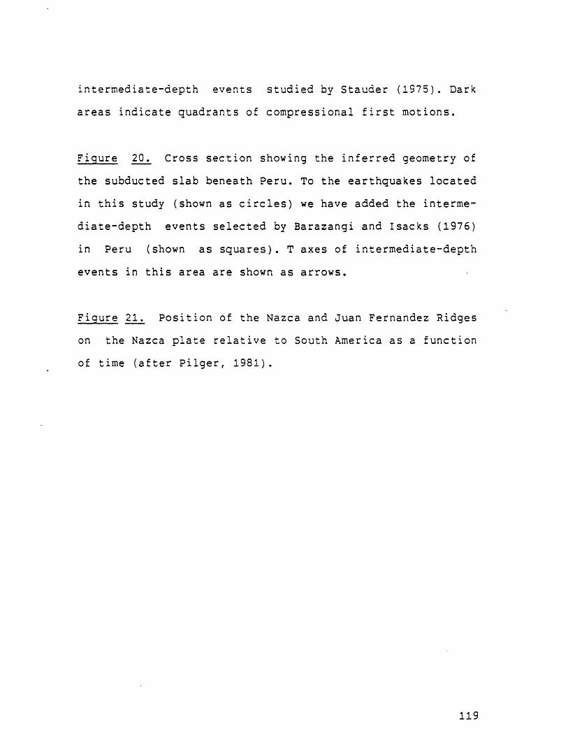
intermediate-depth events studied by Stauder (1975). Dark

areas indicate quadrants of compressional first motions.

Fiqure 20. Cross section showing the inferred geometry of

the subducted slab beneath Peru. To the earthquakes located

in this study (shown as circles) we have added the interme-

diate-depth events selected by Barazangi and Isacks (1976)

in Peru (shown as squares). T axes of intermediate-depth

events in this area are shown as arrows.

Fiqure 21. Position of the Nazca and Juan Fernandez Ridges

on the Nazca plate relative to South America as a function

of time (after Pilger, 1981).

119

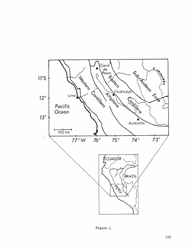
110S

120

130

Figure 1

120

P E R U

1 UNC , POC

MAR

PAC

PAG

PAM

'ATO

11*s

120

130

760 750 740

Figure 2

PacificOcean

770W

15

10

u-5

0

10

C

U-

I I14 16

I I I |18 20 22 24

Epicentral Location Change (km)

I I I I 8 1 1

02 4 6 8 10121 1

14 16I I 2 1

18 20 22 24Focal Depth Change (km)

Figure 3

122

Vp /Vs =1.75

I I I I 1 I2 4 6 8 10 12

Figure 4

123

HUANCATO EXPERIMENT.

77W 75WFigure 5

11s

12S

13S

115

12 S

13S

77W 75WFigure 6

300

Distance from Trench

Figure 7

5000,

0

6000

coastI I

501

I H liii! Ill

100

150

-200

00

00 % 0

o o o0 0 0~0) 00 00 0 0

0 0 00 0

1 o o o11

100 200 400 500 600

Figure 8

120S-Ad-

~.Huancayo*L.3

Figure 9

75* W

128

10 -Q000

15 - o 0 0-

20 -0 0

250 10 20 30 40 50 60

KM

Figure 10

129

I * June 4, 1980Aoy 20, 1980 12h-37'

HuOyIopaolao Co-1osite Acy 31. 1980 Huoylooiono EventFault-Pione Solution June 4, 1980June 9, 1980

(a)

Y130x

x

7-24-69

(C)

Figure 1

130

May 15,19803h:52'

Event in theHigh AndesNear StationPAM

Figure 12

11S

12S

13S

77W 75W

Figure 13

May 15, 1980May 20,1980May 24, 1980May 25, 1980June 4, 1980June 7 1980

Teleseismic Eventin the Sub-Andes

7h: 57'2 h:48'7h:36'

23h: 20'6 h: 22'5h:07'

Events in theSub-Andes

Figure

June 3, 198010h :43'

Event in theSub-Andes

Figure 15

-10'

0 000

00

ooD G 15'

o00

I 20*. 70,

Figure 16

135

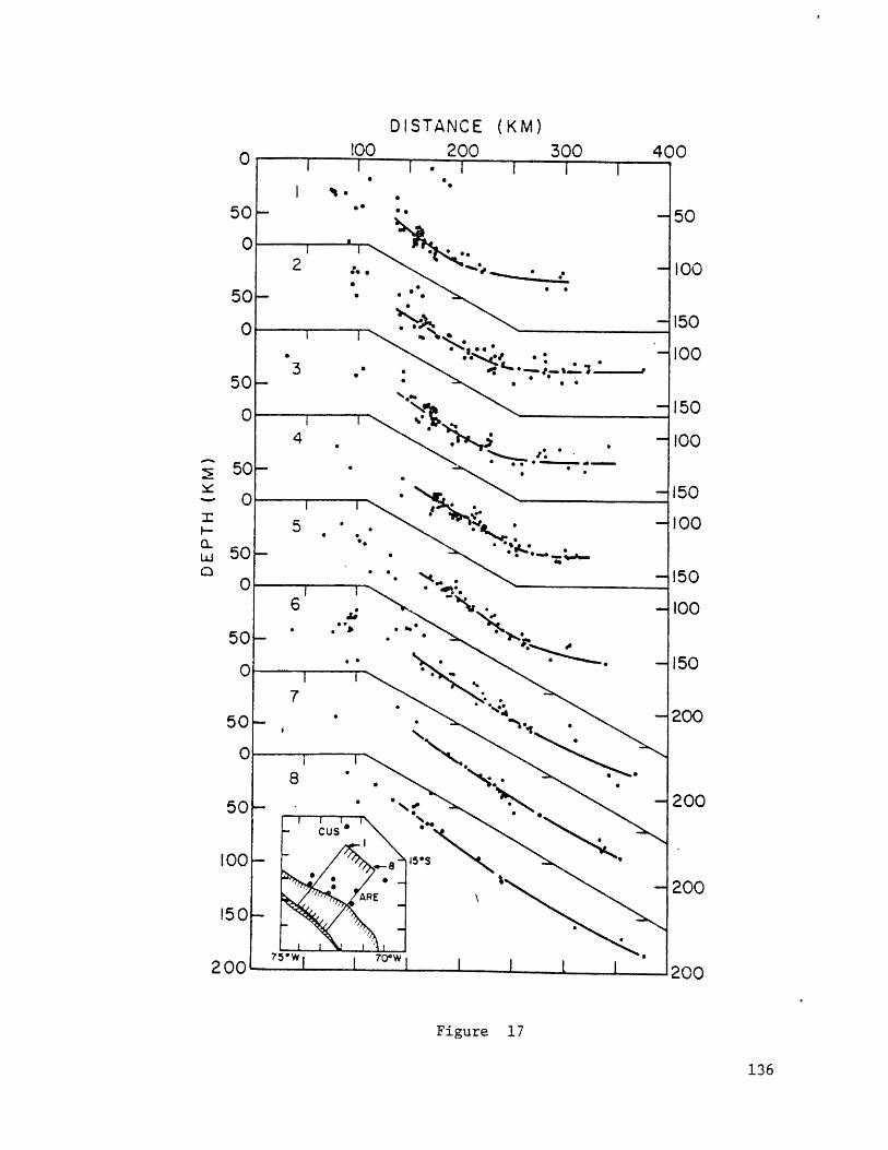
DISTANCE400

-50100

150

100

150

100

150

100

150

100

150

200

200

200

200

Figure 17

136

(K M)

0u June 10,1980 June 10. 1987h:42

l2h: 06'

00

0 O0O

May 22. 19802h:28'

June 10, 19808h:47'

Figure 18

"iS

125

13S

77W 75W

Figure 19

5000

0

6000

coast

0.100-

150

0 100 200 300 400 500 600

Distance from trench (km)

Figure 20

130 0 W 1200 110) 1000 904 800 70* 600

10*

20*

30*

400S

Figure 21

Chanter 4

Introduction

Long period surface waves have been used frequently

to determine the source mechanism and focal depth of earth-

quakes. Early studies, where the observations were compared

to theoretical results on a trial-and-error basis (eg. Tsai

and Aki, 1966; Weidner and Aki, 1973) have been replaced by

efficient inversion methods in the framework of the moment

tensor inversion formulation (Gilbert, 1970; Mendiguren,

1977; McCowan, 1976). Inversion of the moment tensor com-

ponents from Rayleigh waves has been applied succesfully to

a number of earthquakes in different parts of the world

(eg. Kanamori and Given, 1982; Patton, 1978; Romanowicz

1981; Trehu et al 1981). If the complex spectrum is avail-

able, the inversion is linear and yields a unique solution.

If only the amplitude spectra is available, the method

requires the solution of a system of non-linear equations

using an iterative least-squares scheme. Furthermore,

independent information on the source mechanism is

required, usually from body wave data, to constrain the

direction of slip on the nodal plane, which the amplitude

data alone cannot discriminate.

141

To form the complex spectrum, however, the observed

phase must be corrected for the propagation effects of

phase velocity. For periods between 20 and 100 seconds, the

period range most frequently used, phase velocities depend

largely on the crustal structure along the path and, there-

fore, vary greatly for different paths. To perform the

linear inversion, phase velocities must be known with an

accuracy of about 0.5% (Aki and Patton, 1978). Worldwide

regional values of phase velocities are not known yet well

enough to predict accurate phase velocities for any given

wave path on the surface of the earth. This lack of accu-

rate regional phase velocities has severely limited the

application of the moment tensor inversion on a routine

basis for cataloguing or scientific purposes.

The objective of this paper is to present a new method

to perform the moment tensor inversion using only the

amplitude spectrum. The method is an extension of the

scheme suggested for the linear inversion by Romanowicz

(1982a). While not completely eliminating the non-linearity

of the inversion, the proposed method offers some distinct

advantages over that proposed originally by Mendiguren

(1977). It is substantially faster than the traditional

approach (eg. Mendiguren, 1977; Kafka and Weidner, 1979)

and, as shown by Romanowicz (1982a), it eliminates some of

the errors and biases in the data.

142

Examples of earthquakes in the North Atlantic, Central

Asia, and North America show that encouraging results are

obtained using Rayleigh-wave amplitude data as a means of

source parameter and focal depth retrieval. It is impor-

tant to be able to retrieve this information for many

events in the magnitude range 5 to 5.5 that are not large

enough to produce adequate body waves at sufficiently

numerous teleseismic stations, whereas they yield fundamen-

tal mode Rayleigh waves that are well above the noise

level.

The Method

The observed spectrum, u(w,9,r), of vertical-component

Rayleigh waves on a flat layered medium due to a point

source and observed at a distance r, and azimuth 9, is

related to the source spectrum A(w)eio(w) by:

u(w,O,r) = S(w). I(w). e-ser/cteve- Ir- A((o)eiJO(*) (1)

where I(w) is the instrument response, and C(w) and I are,

respectively, the average phase velocity and attenuation

coefficient along the propagation path as a function of

frequency w. The complex function S(w) contains the geomet-

rical spreading factor and other constants.

143

Once corrected for propagation effects and instrument

response, the observed complex source spectrum can be

expressed as a linear combination of the moment tensor com-

ponents Mij (Mendiguren, 1977) as:

A(w)eie*( .6) = a + ij (2)

where,

a = Mzz(G 2-G1 ) - (Myy-Mxx)Glcos29 + 2MxyGsin2G(3)

t = MxzG 3cosO + MyzG 3 sino

The variables G1 are the excitation functions for a given

earth model and have a non-linear dependence on frequency

and depth. Equation (3) implies that IM,1 =0, i.e. the

earthquake is assumed to be a point source with no net vol-

ume change (Mendiguren, 1977; Patton, 1978).

In the scheme originally proposed by Mendiguren (1977),

the observed amplitude spectrum, A=(a 2+p2)11 2, is used to

invert for the moment tensor elements in a and f. This

non-linear system of N equations, where N is the number of

stations used times the numbers of frequencies sampled, is

solved at different trial depths h,. The residuals in the

least-square sense of these successive inversions are then

plotted as a function of depth; true focal depth is inter-

preted as that where the minimum in the residual curve

occurs.

144

An alternative approach to invert for the moment tensor

components can be obtained following the two-step procedure

suggested by Romanowicz (1982a) for the linear moment

tensor inversion. We recognize that equations (3) are of

the form:

a(Wk,6) = Ak + Bkcos 29 + Cksin29(4)

A(wk,6) = Dkcos9 + Eksin9

where the quantities Ak,Bk,...Ek are uniquely determined at

each frequency Wk by the uniqueness of the Fourier expan-

sion in the variable 6 (Romanowicz, 1982a) Note that

equations (4) are linear and completely decoupled from

depth-dependent terms, and are only a function of frequency

and azimuth. The relations between the parameters

Ak,Bk,...Ek and the moment tensor elements are then as fol-

lows:

Ak = Mzz(G 2 (wk,h)-G1(Wkh)

Bk = -(Myy-Mxx)G1(wkh)

Ck = 2MxyG1(wkh) (5)

Dk = MxzG 3 (wk,h)

Ek = MyzG 3 (wkh)

Expressing the observed amplitude spectrum A as:

A 2 (wk) = (Ak+Bkcos26+Cksin26) 2 + (DkcoSO+EksinO) 2 (6)

145

it is possible to proceed in two steps to determine the

moment tensor elements. First, the non-linear system of

equations (6) is solved at each frequency Wk to determine

the quantities Ak,Bk,...Ek. Once these parameters are

obtained for each of the frequencies selected in the inver-

sion (wk=01,W2,---Wn), the system of equations (5) can be

solved for the moment tensor components M1j at each desired

trial depth hi. The focal depth is interpreted as that

where the minimum residual occurs.

For example, to solve for the component Mzz, the system

of equations,

Ak = Mzz(G 2 (wk,hi)-G1(Wk,hi)) (7)

is solved for different values of depth, h,. The residuals

in the least square sense are then plotted as a function of

depth to determine the minimum. Thus, the sensitivity of

each of the moment tensor elements due to changes in depth

can be monitored separately.

As was pointed out by Mendiguren (1977), there is an

inherent limitation in using only the amplitude spectra of

Rayleigh waves to determine the source mechanism. Using

amplitude spectra alone, it is not possible to determine

the sense of direction of slip on the fault plane. Thus, it

is not possible to differentiate, for example, between a

pure thrust and a pure normal fault. Furthermore, since the

radiation pattern of Rayleigh waves has a two-fold

146

symmetry, the solution can be rotated by 1800 and still

satisfy the data. Additional information, usually in the

form of a few first motion data or geological information

is required to constrain the fault-plane solution.

Advantages of the method

While the non-linear character of the method is not

totally eliminated, the advantage over the classical

approach is threefold. First, similarly to the case of com-

plex spectra (Romanowicz, 1982a), this procedure eliminates

biases arising from innacurate propagation corrections

whose dependence on azimuth is orthogonal to the sub-space

spanned by the functions 1,sinO,cosG,...cos49. This can be

seen when the expression for A2 (equation 5) is expanded

into a linear combination of trigonometric functions. Since

the variations with azimuth of the errors in amplitude are

more erratic than those of the phase, errors are reduced

less significantly for the amplitude than for the phase,

where the highest order trigonometric function not elimi-

nated is in 26

Secondly, we can monitor the variance as a function of

depth for each of the five moment tensor components inde-

pendently. This is very useful to constrain focal depth

since some of the moment tensor components are more sensi-

147

tive to variations in depth than others (eg. Patton, 1980;

Romanowicz, 1981).

Finally, from a purely computational point of view, this

approach simplifies considerably the inversion process.

The advantage is that instead of performing a non-linear

inversion at each trial depth, an average of 10 to 12 inv-

ersions if we want a large and closely sampled depth inter-

val, the non-linear scheme is used in the first step only

once at each of the frequencies selected (usually, six to

eight frequencies distributed over a broad frequency range

suffice). Furthermore, the number of equations in the

non-linear procedure is substantially reduced. In the tra-

ditional approach, the number of equations to solve at each

trial depth is equal to the number of frequencies sampled

times the number of stations. In the proposed method, how-

ever, the number of non-linear equations to solve at each

frequency reduces to only the number of stations used. From

our experience, the inversion was 20 to 30 times faster

using the two-step method. The second step of the inver-

sion is a simple linear procedure that only increases

computational time marginally when the number of trial

depths is increased. This enables us to closely scan a

larger depth range without being penalized by long computa-

tion times.

148

Examples of the Application of the Method

In this section several examples of the application of

this moment tensor inversion method are presented. The

results of the moment tensor inversion are compared with

solutions obtained from body wave modelling data, when the

latter are available. The epicentral data of the events

studied are given in Table 1.

The 1982 New Brunswick Earthquake

On January 9, 1982, a moderate-size earthquake

(mb= 5 .7 ) occurred in the central part of the province of

New Brunswick, Canada. The geographic location of this

event provides an excellent opportunity to invert for the

source parameters from the amplitude spectra of Rayleigh

waves using high-quality digital seismograms (Figure 1). A

large fraction of the Seismic Research Observatiories

(SRO), Modified Seismic Research Observatories (ASRO), and

digital WWSSN stations are located in North America,

Europe, and South America. Complemented by stations from

the WWSSN and Canadian networks, digitized manually on a

table-top digitizer, they provide excellent station cover-

age in azimuth.

The moment tensor inversion was performed using nine

periods in the range of between 68 and 26 seconds. The res-

iduals of the inversion as a function of depth are shown in

149

Figure 2. A clear minimum centered at a depth of about 8 km

indicates that the focal depth is in the order of between 4

and 10 km. At a focal depth of 8 km, the solution is an

almost pure dip-slip mechanism oriented in a north-south

direction (Figure 3). This solution agrees closely with the

results obtained by Nabelek et al (1982) from the simul-

taneous inversion of short and long period body waves

(Figure 3). For this solution, the value of the moment

tensor elements Mxz and My. is negligible compared to the

other three independent components (Table 2). In light of

this fact, we can apply the constraints Mxz=Myz=0 in the

inversion. These constraints are equivalent to constraining

the fault mechanism to be a pure double couple and, either,

a pure strike-slip on a vertical fault plane, or a pure

dip-slip on a fault plane dipping at 450 (Kanamori and Giv-

en, 1982). Performing the inversion under these

constraints yields a sharper residual- versus-depth curve.

The resulting fault plane solution at a depth of 8 km shows

a pure dip-slip mechanism with nodal planes oriented

north-south.

As mentioned before, one of the advantages of the method

proposed here is the possibility of monitoring independent-

ly the variation of the residuals in the inversion for each

of the moment tensor elements. Figure 4 shows the residuals

for the moment tensor elements that form the real part of

the spectrum. As discussed by Patton (1978), the moment

150

tensor components that form the imaginary part of the spec-

trum are not very sensitive to changes in depth.

The residual-versus-depth curves of the individual

moment tensor elements show that Mzz is the most sensitive

to focal depth variations. It exhibits a sharp minimum at 8

km that rises suddenly for depths larger than 10 km. The

other two components are less sensitive to depth. Myy-Mx

shows a broad minimum centered at 10 km and MXY is virtual-

ly constant as a function of depth.

The sharp reduction in residuals constraining the depth

to be between 5 and 10 km, and the excellent agreement of

the focal depth and source mechanism gleaned from the

inversion with those obtained by Nabelek et al (1982) using

body wave data are the result of two important factors.

Firstly, most of the paths from source to station are short

and lie generally within a single tectonic province. Sec-

ondly, the results reflect the quality and high

signal-to-noise ratios of the digital seismographic

stations used. Clearly, the possibility of applying moment

tensor inversions on a routine basis will become feasible

when world-wide coverage of digital stations improves.

An Aftershock of the 1974 Gibbs Transform Fault Earthquake

This earthquake is an aftershock that occurred in the

Gibbs transform fault in the North Atlantic, a few days

after the large 1974 earthquake studied in detail by

151

Kanamori and Stewart (1978). The body wave magnitude

reported by the International Seismological Center for this

event is 4.9.

This event is a good example of an earthquake for which

a fault plane solution could not be obtained because it did

not produce large enough body waves to be observed at

enough WWSSN stations at teleseismic distances. However,

very clear Rayleigh waves were recorded at a number of

stations around the epicenter offering adequate azimuthal

coverage to perform a moment tensor inversion from them

(Figures 5 and 6). The results of the moment tensor inver-

sion applied using a period range of between 55 and 26 sec

shows excellent agreement to the solution obtained by

Kanamori and Stewart (1978) for the main shock (Figure 7).

The inversion converged to the same solution regardless of

the orientation of the nodal planes in the starting sol-

ution. Only when the initial guess on the value of the

scalar moment was wrong by about a factor of 5 did the sol-

ution fail to converge to the fault plane solution shown in

Figure 7. The residual versus depth curve shows that the

earthquake occurred at a depth of between 5 to 15 km

beneath the sea floor (Figure 8). Although the curve does

not show a sharp minimum, it resolves the depth consider-

ably better than using the method suggested by Mendiguren

(1977). (Figure 8).

152

Although we do not constrain the solution to be a

double-couple source, the solution obtained at a depth of 9

km is almost a pure double-couple; the value of the B axis

is about one and one-half orders of magnitude smaller than

that of the P and T axes.

An earthquake in the Tien Shan

This earthquake occurred in the Tien Shan mountains

in central Asia on June 24, 1972. The focal depth of this

event was studied by Romanowicz (1982b) using long-period

body wave modelling following a fault-plane solution by

Roecker et al (1980). Romanowicz (1982b) obtained a focal

depth of approximately 15 km based on the comparison of

theoretical and observed body waves. The depth reported by

ISC was 47 km.

The moment tensor inversion of Rayleigh wave amplitude

data yields a focal depth of 15 km (Figure 10) in agreement

with the result obtained using body-wave modelling. The

resulting fault plane solution shows a dip-slip mechanism

with some strike-slip motion. It agrees in general with the

result of Roecker et al (1980) although it violates a few

first motion data (Figure 9). As in the previous examples,

the solution is independent of the initial guess used in

the inversion and shows better depth resolution than the

traditional approach (Figure 10).

153

Summary

A new approach to invert for the moment tensor compo-

nents using only the amplitude spectra of vertical compo-

nent Rayleigh waves is discussed. The method consists of

two steps: First, the amplitude spectra are decoupled from

their depth dependent terms and fit with a smooth function

of azimuth at each frequency selected for the inversion.

This has the effect of eliminating some biases and errors

in the data. In the second part, each of the five independ-

ent moment tensor components is monitored separately at

various trial depths. True focal depth is then determined

as the minimum in the variance versus depth curve. Encour-

aging results are obtained applying the method to

earthquakes in Central Asia, North America, and the

Mid-Atlantic Ridge. The method is shown to be a useful

tool to determine the source parameters of a number of

local or intraplate earthquakes for which a poorly con-

strained solution is obtained from body wave data alone,

and when the absence of accurate regional phase velocities

precludes the use of a linear moment tensor inversion.

154

TABLE 1

HYPOCENTRAL DATA OF EARTHQUAKES STUDIED*

EVENT LOCATION

Gibbs TransformFault

Tien ShanMountains

New BrunswickEarthquake

DATE

11/16/74

06/24/72

01/09/82

LAT

52. 64N

LON

32.15W

36.30N 69.69E

46.98N 66.66W

DEPTH(ISC)

26

47

7

ESTIMATEDDEPTH mb

9 4.9

15 5.9

8 5.7

*All data from the ISC catalog except for the New Brunswickevent which is from the USGS Preliminary Epicentral Determinations.

155

Table 2

RESULTS OF MOMENT TENSOR INVERSION

New Brunswick Event Depth=8 km

Mzz = -1.04x10 2 4

Myy-Mxx = -1.24x10 2 4

Mxy = -1.19x10 2 3

Mxz = 2.80x10 18

Myz = -2.64x10 18

dynes/cmIf

I'

n,

n,

Gibbs Transform Fault Event Depth=9 km

M = 1.57x10 2 2

M -Mxx = 7.52x10 2 2

Mxy= -1.60x10 2 3

Mxz= -1.69x10 18

Myz= -7.09x10 1 8

Tien Shan Earthquake

Mzz= 8.99x10 24

Myy-Mxx = -7.37x10 2 4

My= 3.46x10 2 4

Mxz = -3.24x10 2 4

My Y= -1.81x10 2 4

dynes/cm

Depth=15 km

dyne s/cmn,

I,

nI

II

156

Figure Captions

Figure 1. Location of the January 9, 1982 New Brunswick

event. Squares indicate the seismographic stations used in

the inversion.

Figure 2. Residual versus depth curve for the moment

tensor inversion of the New Brunswick earthquake. Open cir-

cles for the unconstrained inversion, closed circles for

the constrained inversion (Mxz=Myz=O). Residuals are nor-

malized to the maximum value in each case.

Figure 3. a)Closed circles are compressional first motions

of P waves plotted on a lower-hemispheric projection. Solid

line is the fault plane solution obtained from the uncon-

strained moment tensor inversion, dashed line is the sol-

ution of the constrained inversion, and dotted line is the

solution determined by Nabelek et al (1982) inverting body

wave data. b) Rayleigh-wave amplitude radiation pattern at

a period of 50 seconds.

Figure 4. Normalized residuals versus depth for the three

moment tensor elements in the real part of the spectrum.

157

Figure 5. Location of the earthquake in the Gibbs trans-

form fault and the stations used in the moment tensor

inversion.

Figure 6. Examples of Rayleigh waves recorded at vaious

WWSSN stations from an earthquake in the Gibbs transform

fault (mb = 4.9).

Figure 7. a) Source mechanism of the aftershock in the

Gibbs transform fault obtained from the moment tensor

inversion (dashed line). Solid line is the fault plane sol-

ution determined by Kanamori and Stewart (1976) for the

main shock. b) Rayleigh-wave amplitude radiation pattern

at a period of 40 seconds.

Figure 8. Normalized residuals versus depth for the Gibbs

transform fault event. Closed circles using the method pro-

posed in this paper, squares using the traditional method.

Figure 9. a) Fault plane solution of the earthquakes in

the Tien Shan. Closed circles are compressional first

motions and open circles dilatational first motions. Solid

line is the fault plane solution (Roecker et al, 1980),

dashed line is the solution of the moment tensor inversion.

b) Amplitude radiation pattern of Rayleigh waves for a

period of 70 seconds.

158

Figure 10. Normalized residuals versus depth for the Tien

Shan earthquake. Closed circles using the method presented

in this paper, squares using the traditional approach.

159

Figure 1

160

1.0 -- - - - - - - - -

.8--

F-

D .6(

C/)

0

.2 -

5 10 15 20

Depth (kin)

0 Unconstrained* Constrained

25 30

Figure 2

(Mxz=myz=o)

UNCONSTRAINED MOMENT TENSOR INVERSION

CONSTRAINED MOMENT TENSOR INVERSION (MXy=MyzO)

E..........ODY WAVE INVERSION (NABELECK ET AL, 1982)

Figure 3os

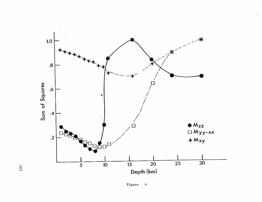
1.0

.8

+G4AI

g .6 -

cI!

E .4 -

O o Mzz(--/' /Y -X

.2+ MY

5 10 15 20 25 30

Depth (km)

Figure 4

-120

-60

Earthquake in the Gibbs Transform

Nov 1 6,1.974Figure 1

180

120

60

Fault

Mb 4.9

ujw9 ainVTAd

-AN V

~100

~1vWN

dOO

JXO0

jIIJ

Gibbs Earthquake

Rayleigh Waves

T - 40 sec.

% -

%-

-- p

I~

-I*~

4

(b)

P= I .14 B=0.07 T=I .04 x 10 24dynes cm.

(a)

Kanamori and Stewart (1976)

Amplitude Inversion

Figure 7

Earthquake in the Gibbs Transform Fault

10

*1"""urn,.

c-

U)

m----m---,nu~~ U

I/

/

i I Ii I

10 15

De pth

20 25

(k m)

Figure 8

167

I Ii.

30

,Rayleigh WavesT-50

(a) (b)

Figure 9

00

I I II I I I I10 20 30 40 50 60 70 80 90

Figure 10

169

Chapter 5

Introduction

Linear moment tensor inversion in the period range of

90 to 20 sec has been succesfully applied to retrieve the

source parameters a-nd focal depths of earthquakes in Cen-

tral Asia (Patton, 1978, 1980; Romanowicz, 1981), the north

Atlantic (Trehu et al, 1981), and the Java trench (Fitch et

al, 1981). Our objective in this paper is to implement

this technique for earthquakes in the Central Andes. One

of our original intentions in this study was to use the

linear moment-tensor inversion method to retrieve the focal

depth and source mechanism of a number of relatively small

events (between 4.8 and 5.5 mb) that occur in the northern

Altiplano, where normal faulting has been observed on

Quaternary sediments (e.g. Lavenu, 1979). This proved to

be difficult, however, because none of these events were

not recorded at a large enough number of stations around

the world due to the long epicentral distances.

For earthquakes in this area the azimuthal coverage of

WWSSN stations is good but the paths from the source to the

station are considerably longer than those used in the

studies mentioned before. We have studied seven earthquakes

170

occurring within the crust of the central Andes, for which

the focal depth and fault-plane solution have been con-

strained comparing the observed body-wave signals with

theoretical waveforms (Chapter 2). This will permit us to

judge the accuracy of the results of the moment tensor

inversion.

A reference-point method, as described by Patton (1980),

is implemented using a cluster of events to obtain accurate

phase velocities to stations around the world. We explore

the possibility of applying the inversion routinely, by

investigating how far one can select events away from this

reference point and still be able to invert succesfully for

the moment tensor and focal depth, using the same phase

velocity measurements. Here, we will judge the goodness of

fit of the moment tensor and depth estimates by their

agreement with the results of the body-wave analysis.

Method

The linear inversion of the moment tensor from the

complex spectra of vertical-component Rayleigh waves has

been discussed extensively in the literature (McCowan,

1976; Mendiguren, 1977; Aki and Patton, 1978, Patton,

1978). In this paper we use a modification of the linear

moment tensor inversion method proposed by Romanowicz

171

(1982a), which significantly improves the resolution of the

focal depth and the source mechanism. The algorithm is

essentially the same as the one used to invert the moment

tensor using only the amplitude spectra of Rayleigh waves

that was presented in Chapter 4.

As shown in Chapter 4, we proceed with the inversion in

two steps. First, the real and imaginary part of the

spectra corrected for inelastic attenuation and the

dispersion of surface waves, are considered a continous

function in azimuth and expressed only as a function of

azimuth, &th., and five constants Ak,Bk,Ck,Dk,Ek, at fre-

quency Wk (Equations 1 through 5 in Chapter 4). In the

case of the linear moment tensor inversion, however, since

we recover both the phase and amplitude spectra, the real

and imaginary parts of the spectrum can be separated.

Therefore, the constants Ak,Bk,...Ek are determined at

every frequency sampled by simply solving the two systems

of linear equations shown in Equation 4.4. Once these con-

stants are determined, Equations 4.5 are used to solve for

the moment tensor components at various trial depths. The

least square residuals obtained for these different trial

depths in Equations 4.5 are plotted as a function of depth

and the minimum in this curve is interpreted as the best

estimate of focal depth. The P, B, and T axes of the fault

plane solution correspond to the eigenvectors of the

diagonalized moment tensor (Mendiguren, 1977). As dis-

172

cussed by Mendiguren (1977) the success of this method

hinges on our ability to define a clear and significant

minimum in the residuals-versus-depth curve.

Romanowicz (1982b) has shown convincingly that this

method is more robust than inverting directly for the

moment tensor elements from Equation 4.3. Using this

two-step procedure, it is possible to eliminate most of the

errors and biases in the data that are not 1 periodic in

azimuth from the source. These errors and biases introduced

by using inexact propagation corrections, as well as by

errors in the location and origin time of the event, are

not coupled with the source parameters and depth in the

inversion, and tend to flatten the residual curve.

Data Analysis

Earthquakes Studied

We have selected seven crustal earthquakes with

body-wave magnitudes of between 5.7 and 6.1 that occurred

in the Andes within the South American plate (Figure 1).

The fault-plane solution and focal depth of the earthquakes

used in the study have been constrained using body-wave

modelling in Chapter 2. This will help provide an inde-

pendent test on the accuracy of the focal depth and source

173

mechanism obtained using the linear moment tensor

inversion. The seven events selected are those which showed

good quality long-period data on vertical component

seismograms on WWSSN stations distributed around the

epicenter (Figure 2). The epicentral data of these events

is shown in Table 1.

Signal Analysis

The main Rayleigh wave train was identified in the

seismogram and digitized on a table-top digitizer over a

time window corresponding to a group velocity of between

4.2 and 2.2 km/sec, at evenly spaced intervals of about one

second. The digitized time series were plotted and compared

with the original seismograms to detect any errors in the

digitization procedure. The time series were then detrended

and fourier transformed, and the instrument response

removed using the instrumental constants supplied by a par-

ticular station (Hagiwara, 1958). To eliminate background

noise present at the station and signal-generated noise

such as body-wave interference, multipathing, and scatter-

ing, the time series were filtered using a time-variable

filter (Landisman et al, 1969). This is a two-step proce-

dure that requires, first, the determination of group

velocity. Group velocities were obtained using a

moving-window analysis that yields the energy contained in

a windowed portion of the seismogram on a

174

velocity-versus-period plot. The group velocity of the

fundamental-mode Rayleigh wave is identified by contouring

the region where the maximum energy arrives. Figure 3 shows

energy plots and contoured group velocities for various

seismograms. The second step consists of applying a

band-pass time-variable filter to the time series that

passes only wave packets arriving at the group velocity of

the fundamental-mode Rayleigh waves. This filtering allows

us to eliminate noise of the same frequency band as the

seismic signal of interest, without distorting the original

time series (Figure 4). The time-variable filter has the

effect of smoothing both the amplitude and phase spectra,

without introducing phase delays or distortions (Figure 5)

(Weidner, 1972).

The Earth Model

The application of the moment tensor inversion

requires the prescription of an earth model in the source

region, to estimate the excitation functions. We have used

the crustal velocity structure suggested by Ocola and Meyer

(1973) for the Eastern Cordillera over a Gutenberg earth

model. The thickness of the crust has never been directly

measured in the sub-Andes. Based on phase-velocity meas-

urement of surface waves, James (1971) suggests a crustal

thickness of 70 km for the Altiplano. Since most of the

earthquakes selected occur in the sub-Andes and the crust

175

probably thins to the east, we have used a mean crustal

thickness of 50 km to calculate the excitation functions

(Saito, 1967).

Initialization of the Propagation Corrections

The Reference Point Method

As discussed above, to apply the linear moment tensor

inversion we need to know the propagation corrections very

accurately. Aki and Patton (1978) showed that phase veloci-

ties must be known to within 0.5% to succesfully invert for

the moment tensor and focal depth. Romanowicz (1982b) sug-

gests that using the modified scheme described above, the

accuracy with which we should know the phase velocity is

relaxed, and shows that an event with well-constrained

focal mechanism and depth can be succesfully used to obtain

an initial estimate of phase velocities.

To initially establish the propagation corrections from

a cluster of events in Central Asia, Patton (1978) used the

double-event parameter search developed by Weidner and Aki

(1973). This method, however, requires two events with dif-

ferent fault-plane solutions located close to one another,

and is cumbersome and time-consuming. Here, we initialize

the propagation corrections as follows: First, we use the

176

non-linear moment tensor scheme described in Chapter 4 to

obtain the source mechanism and focal depth of event 1.

This event was selected because it is very well recorded in

most of the stations of interest around the epicenter. Fur-

thermore, this event produced a surface rupture (Philip and

Megard, 1975; Chapters 2 and 3) which will help in judging

the results of the non-linear inversion method. If the

results of the non-linear inversion are compatible with the

body-wave study and the geological information, we can

safely assume that the surface wave data is of sufficient

quality to obtain a first estimate of the propagation

parameters. Then, following the reference-point technique

developed by Patton (1978, 1980), we refine the estimation

of phase velocity and attenuation by inverting for the

depth and moment tensor of other events that occur closeby.

Once the source parameters of these new events are

obtained, these earthquakes are added to the reference

point and the propagation correction is updated and

improved using the maximum-likelihood estimator developed

by Pisarenko (1970).

We can visualize this method by considering that the

earth acts as a linear operator, reiU, to the propagation

of surface waves. The input signal to this system is the

source spectrum and the seismogram represents the output.

The amplitude and phase response of the system, namely the

effect of attenuation and phase velocity along the path,

177

can be obtained by taking the spectral ratio of the output

spectrum to that of the input. Earthquakes located in a

tight cluster and registered at the same seismographic sta-

tion represent independent inputs to a common "earth opera-

tor" or transfer function (Figure 6). Assuming that the

noise at both the source and the station obeys Gaussian

distributions independent from each other, the method

developed by Pisarenko (1970) yields the maximum likelihood

estimation of the transfer function ,re'^, given n inde-

pendent observations. Here, we treat, earthquakes 1,2, and

3, occurring in a tight cluster in central Peru as the

events forming the reference point.

Results of the Amplitude Inversion

The moment-tensor inversion of the amplitude spectrum

of event 1 was performed sampling a set of eight periods

between 80 and 30 sec. The results of the non-linear

moment-tensor inversion for event 1 show good agreement

with the results of the body-wave modelling (Figure 7). The

normalized residuals shown in Figure 7 show a minimum cen-

tered at about 8 km, in good agreement with a focal depth

of 5 km obtained in Chapter 2 from body wave modelling.

The residuals increase rapidly away from the minimum and

after a depth of around 50 km, they decrease slowly forming

a broad minimum in a shape that is characteristic of shal-

low events (Patton, 1978; Romanowicz, 1980). The strike of

178

the resulting source mechanism agrees to within 150 with

the results of the body wave data. However, the orien-

tation of the east-dipping fault plane is not well

constrained and violates a few of the first motion data.

The resulting source mechanism agrees with the general ori-

entation and direction of slip determined from the

body-waves.

These results confirm that the Rayleigh-wave data col-

lected for this event may be used to make an initial esti-

mate of the propagation parameters. To estimate the phase

velocities we use a single-event technique (e.g. Aki and

Richards, 1980) taking the spectral ratios between the

observed spectra and the theoretical source spectra. In

this case, the theoretical source spectra was calculated

using the fault parameters determined from the body-wave

study.

Adding new events to the reference point

Event 2 This earthquake occurred a couple of months before

event 1. The fault-plane solutions of these two events are

virtually identical and body wave modelling suggests they

occur at practically the same depth. Not surprisingly, the

Rayleigh wave trains of these two earthquakes are very sim-

ilar. Using the phase velocities calculated from event 1

and a set of periods spanning the range between 70 and 26

179

seconds, we applied the linear inversion method to obtain

the moment tensor and focal depth. The results show a

sharp minimum centered at a depth of 8 km and the resulting

source mechanism agrees with the first motion data to with-

in 200 in strike. (Figure 8).

To refine the phase velocities measured from the refer-

ence point, the theoretical source spectrum for the mech-

anism obtained in the inversion of event 2 is combined with

that of event 1.

Event 3 This earthquake is located about 50 kilometers east

of events 1 and 2 (Figure 1). The phase velocities

obtained from the stacking of events 1 and 2 were used to

correct the observed spectra of event 3 for propagation.

The inversion was then applied using a period range of

between 80 and 30 seconds. Figure 9 shows the residual ver-

sus depth curve and the resulting source mechanisms

compared to first motion data. The minimum occurs at a

depth of 15 km which is somewhat shallower than the depth

of 18 km obtained in Chapter 2. This difference in focal

depth, however, certainly falls within the errors of both

methods. The resulting source mechanism shows thrust fault-

ing with a component of right-lateral strike-slip motion

also in agreement with the body wave data.

As in the case of event 2, the theoretical spectra for

the resulting source mechanism are calculated and stacked

180

with those of events 1 and 2 to improve the estimates of

phase velocity using the method proposed by Pisarenko

(1970).

In our experience, Pisarenko's formulation works well

down to periods of about 30 sec. As discussed by Patton

(1978), the method does not work as well at shorter

periods, probably because the statistical model used in

deriving Pisarenko's formulas assume an additive Gaussian

noise distribution. For short periods (less than about 30

or 40 sec) the prevalent noise in the signal is due to

scattering and interference which are signal generated and

cannot be modeled by a superposed ambient Gaussian noise.

In these cases, we use a simple phase averaging scheme to

obtain a mean phase delay. The phase velocities resulting

by stacking the data of events 1,2, and 3 are shown in

Appendix 2 grouped by the geographic location of the sta-

tion.

Inversion of Events Away from the Reference Point

Events 4 and 5

These two earthquakes occur within 300 km of the ref-

erence point. For event 4 the residual-versus-depth curve

shows a clear minimum centered at a depth of 6 km, and the

181

_--wo WIN N MIN 11011 " I IN I I - I

resulting source mechanism indicates pure-strike slip

motion consistent with the fault-plane solution (Figure

10). The residual curve for event 5 shows a broad minimum

from about 20 to 40 km centered at a depth of 32 km (Figure

11). The depth resolution for this deeper event is not as

good as for the shallower earthquakes. However, the source

mechanism obtained from the moment tensor inversion shows a

pure dip-slip mechanism that agrees to within 50 in strike

with the one obtained from the first motion data (Figure

11). This is probably due to the excellent azimuthal cov-

erage available for this earthquake. The radiation pattern

of event 5 clearly shows a two-lobed pattern with nodes to

the north and south (Figure 12).

Event 6

This earthquake is located about 700 km northwest of

the reference point. It is the deepest crustal earthquake

obtained in Chapter 2. The inversion shows a

residual-versus-depth curve with a broad minimum from 30 to

50 km. (Figure 13), and as in the case of event 5 the depth

resolution lies probably within ± 8 km. The mid-point of

that broad minimum, however, is centered around a focal

depth of 40 km that agrees with the focal depth determined

on the basis of body-wave modelling. The source mechanism

at a depth of 40 km (Figure 13) shows a thrust mechanism

with a component of strike-slip motion that violates some

182

of the first motion data. The type of faulting mechanism

and the general orientation of the P axes, however, are

consistent with the fault-plane solution.

Event 7

Event 7 occurred in central Ecuador on October 6, 1976

and is located about 1400 km nortwest of the reference

point. The moment tensor inversion was performed using a

period range of between 66 and 30 sec. In this case, the

residual curve does not show a clear and well defined mini-

mum. The depth inferred from the residual reduction is

about 12 km and roughly agrees with the focal depth of 16

km inferred from the body-wave modelling study (Figure 14).

The residual reduction, however, is marginal and probably

indicates that we are reaching the limit of applicability

of the phase velocities obtained from the reference point.

The source mechanism obtained is still compatible with the

first motion data inasmuch the type of thrusting mechanism

and crude orientation of the fault plane solution is

retrieved. The dip of the nodal planes, however, differs

by about 40* from those determined using first motion data.

Figure 15 shows a comparison between the phase velocity

from the reference point to station WES, in the eastern

United States, and the phase velocity computed using the

source parameters of event 7 determined from the body-wave

modelling study. The differences between these two curves

183

are as large as 2% even for the long periods, and this

innacurate propagation correction is reflected in a poor

residual reduction.

In summary, the maximum distance away from the vicinity

of a well established reference point from which the same

phase velocities can be used appears to be not more t.han

about 800 km in the Andes. For events at distances less

than about 800 km, the moment-tensor inversion yields

source mechanisms for which the nodal planes agree with

those obtained using body-wave modelling to within 200, and

focal depths to ± 8 km As shown by Romanowicz (1981) the

minimum in residual-versus-depth curves become less sharp

as one moves away from a well established reference point

and the phase velocity corrections become more and more

imprecise.

A prevalent feature in our results as well as those of

Romanowicz (1981) is the lack of resolution of the moment

tensor inversion method to constrain small strike-slip com-

ponents in dip-slip mechanisms. This is probably due to the

fact that the small lobes in the radiation pattern associ-

ated with them are either buried or exagerated by the

noise.

184

Phase Velocity Measurements

The phase velocities determined in this study show

relatively small variations for stations located in the

same geographical area.(Appendix 2). This is in contrast

with the results of Patton (1978), who shows that large

variations in phase velocity exist even for stations

located in the same general area. Figure 16 compares the

phase velocities determined from Patton's reference point

and those obtained in this study for stations located in

the Iberian Peninsula and the British Isles. Patton's phase

velocities show variations of up to 0.1 km/sec among them.

Even though the paths from the reference point developed in

this study are longer, differences among the measurements

for different stations in this area are comparable. This is

clearly due to the fact that the paths from South American

events travel through the Brazilian Shield and the North

Atlantic region which are much more homogeneous than the

Eurasian continent.

Most of the wave-paths to stations outside South America

and the Caribbean region have a substantial fraction of the

total path length in oceanic terranes. This may explain our

success in retrieving the source mechanism and focal depth

of earthquakes in South America by using the moment tensor

inversion, even though the average path length is about 35%

longer than those from Central Asian earthquakes (Patton,

185

1978; Romanowicz, 1981). In fact, in the period range of 40

to 100 seconds phase velocities measured from the reference

point to any station outside South America vary less than

3.0% among them (Figure 17).

These small changes in phase velocity for various paths

clearly reflect the well known lateral homogeneity of the

oceanic crust and upper mantle (Forsyth, 1975). More

interestingly, however, they also show that the cratonic

South American shield should also be very homogeneous since

the paths to eastern North America, Europe, and Africa have

long portions of the paths over different parts of the

shield (Figure 2). This lateral homogeneity of the

Brazilian shield is clearly shown by the only two pure-path

phase velocity measurements in the South American craton.

Up to a period of 60 sec, the phase velocities to station

NAT in northeastern Brazil, and to station TRN in Trinidad

are virtually identical (Figure 18). We were not able to

determine the phase velocity for periods longer than 70 sec

in the Brazilian shield. The phase velocity measurements

obtained for the Brazilian shield are very similar to those

of the Canadian (Brune and Dorman, 1963) and the Indian

shield (Patton, 1978), except at periods less than about 40

sec long, for which the velocity across the Brazilian

Shield is lower than that of the Indian and the Canadian

shields (Figure 19). The smaller phase velocity at shorter

periods in the Brazilian shield could be interpreted as a

186

result of a slightly thicker crust in the Brazilian shield

than in the Indian and Canadian shields. To our knowledge,

the measurements presented here are the only pure-path pub-

lished phase velocities in the Brazilian shield.

Due to the sparse coverage of WWSSN stations in the

Andes and to the contorted shape of the South American

coastline we were not able to obtain pure-path phase veloc-

ities with trajectories wholly within the Andes. The mixed

path to station LPA in Argentina (RFP-LPA in Figure 20)

crosses the Andes of central Peru, the Altiplano, and a

portion of the Argentinian lowlands. The phase velocity

measured along this path, however, is very similar to the

phase velocity determined by James (1971) for the eastern

part of the Altiplano from the path LPB-CUS (Figure 21).

Summary

In order to test the feasibility of applying routinely

the method of moment-tensor inversion in a particular area

of the world, we developed accurate phase velocity measure-

ments stacking data from a tight cluster of events in cen-

tral Peru using the maximum-likelihood estimator developed

by Pisarenko (1970). These phase velocities were then used

to invert for the moment tensor and focal depth of other

earthquakes in the central Andes, as far as about 1400 km

187

away from the reference point. The results in South America

show that if the distances between the reference point and

the earthquake of interest is less than about 800 km, the

moment-tensor inversion yields results that agree to within

200 with the nodal planes determined using first motion

data and long-period body-wave modelling. The estimated

focal depths appear to be within t 8 km to those obtained

from body-wave studies, and the uncertainty increases with

increasing depth. The one event studied that was located

at a distance of about 1400 km from the reference event

shows a marginal residual reduction for inversions at dif-

ferent trial depths, and the dip of the nodal planes of the

resulting mechanism differs by over 30* with those deter-

mined from the first motion data.

188

TABLE I

LIST OF EARTHQUAKES

Event Date Latitude Longitude Origin Time Depth Magnitude

-11.75

-11.84

-11.62

-14.20

-9.84

-6.79

-0.76

-75.15

-75.10

-74.45

-73.45

-75.55

-76.76

-78.75

STUDIED

Oct. 1,

Jul.24,

May 15,

Oct.15,

Feb.14,

Mar.20,

Oct. 6,

1969

1969

1976

1971

1970

1972

1976

5h 5'

2h 59'

21h 55'

10h 33'

11h 17'

7h 33'

9h 12'

50.0"

20.9"!

55.0"

46.3"

16.4"

48.7"

39.0"

5.8

5.9

5.9

5.7

5.8

6.1

5.7

189

Figure Captions

Figure 1. Map showing surface wave paths from the

epicenter to the WWSSN stations (closed circles) used in

the study.

Figure 2. Location of the earthquakes studied. The number

beside the epicentral locations (stars) indicates the depth

estimated from a body-wave modelling study. Dark areas

indicate compressional first motions on these lower

hemispheric projections of the fault-plane solutions

obtained from the body-wave analysis.

Figure 3. Examples of energy arrival on a period versus

velocity plot. Letters and numbers indicate the energy of a

particular period, Z being the maximum and decreasing 2 db

for every letter. Lines show contours of maximum-energy

arrivals that indicate the group velocity of the fundamen-

tal Rayleigh-wave mode.

Figure 4. Examples of raw and filtered seismograms.

Figure 5. Comparison between the phase and amplitude

spectra of a raw (solid line) and filtered (dashed line)

seismogram.

190

Figure 6. a) Schematic representation ofa linear operator

with n independent samples. b) Lowes' (1970) graphic repre-

sentation of Pisarenko's estimator.

Figure 7. a) Fault plane solution of event 1. Closed cir-

cles indicate compressional first motion and open circles

dilatational on a lower-hemispheric projection. Crosses

represent nodal readings. Dashed line is the solution

determined from a body-wave modelling study (Chapter 2),

and the solid line is the solution obtained using the

moment-tensor inversion. b) Residual-versus-depth curve

resulting from the moment-tensor inversion at different

trial depths. Arrow points to estimate of focal depth from

the body-wave modelling study

Figure 8. Results for event number 2. Symbols as in Figure

7.

Figure 9. Results for event number 3.. Symbols as in Figure

7.

Figure 10. Results for event number 4. Symbols as in Fig-

ure 7.

Figure 11. Results for event number 5. Symbols as in Fig-

ure 7.

191

Figure 12. Radiation pattern of the amplitude spectrum of

event number 5 at a period of 76 sec.

Figure 13. Results for event number 6. Symbols as in Fig-

ure 7.

Figure 14. Results for event number 7. Symbols as in Fig-

ure 7.

Fiqure 15. Comparison of phase velocities to station WES,

in the eastern United States. Open circles represent phase

velocity measured from the reference point. Closed circles

are the phase velocity measured from event 7 using the

one-station method. The theoretical source spectrum for

event 7 was calculated using the focal depth and

fault-plane solution determined comparing observed and syn-

thetic long-period body waves (Chapter 2).

Figure 16. Comparison of phase velocities measured to

stations in the Iberian peninsula and British Isles from a)

Patton's reference point (1980) and b) this study. Note

similarity in paths from South America and large scatter

for Eurasian paths.

Figure 17. Typical phase velocities measured from central

Peru to stations in various geographical areas.

192

Figure 18. Phase velocity measurements on pure-paths

accross the Brazilian shield to station NAT in Brazil, and

TRN in Trinidad.

Figure 19. Phase velocity measured for the Brazilian

shield compared to those of the Indian (Patton, 1978) and

Canadian Shield (Brune and Dorman, 1963).

Fiqure 20. Surface wave paths across the central Andes.

Line indicates the 3000 meter elevation contour.

Fiqure 21. Phase velocity measured from central Peru to

station LPA in Argentina compared with phase velocities for

other Andean paths (James, 1970) and a pure-path measure-

ment in Tibet (Romanowicz, 1982b).

193

Figure 1

194

Figure 195

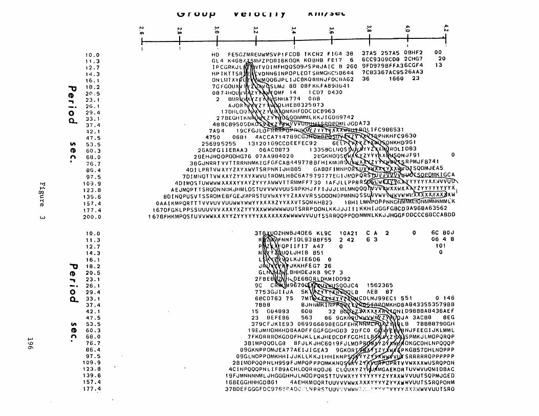
Group Velocity km/sec

10.010.0 HD FESGZMREI.WMSVP1FCQB IKCN2 F164 38 37A5 257A5 001*2 00

11.3 GLI K466" MPZPORI6KOOK KO3NB FE17 6 6CC9369CD8 2CHG7 2012.7 IPCRjL 4TV0INFHQQS09r)SPRJAIC 1 260 9FD979BFFA36CGF4 13

14.3 HP SR .VDNN61NPOPLE0TSRMGHC5B644 7C83367AC9526AA316.1 DNLMTY QQGJPLIJCBKQRIINJFDCF3A62 36 1660 23

18.2 7GIGOUX SLMJ 83 08FKFA69064120.5 0874HQU ZY QMF 14 iCD7 0430

-, 23.1 2 8R U NHA774 068,26.1 AJOR ZY LHE0325073

0 29.4 17DFLOQ zY, NI(HFDOCDCB963q 33.1 27BEGHIKN ZY QONMMLKI G0119742

37.4 48BC69505DK vv412.1 79 9FJOzYYLF963

47.5 4750 0681 4ACCA714789CG P1KHFC9630to 53.5 256995255 1312O169CCDEEFEC92 6EL Z NKHD961

0 60.3 26ADFG1IEBAA3 06AC3873 13358GLIJQS YYZ ROLID83% 68.0 2BEHJNOOPOOHG76 07AA984020 2eGINOQS ZYYY X QNJF91 0

76.7 3BGJNRRTVVTTRRNNMKIGFGFCAB449778BFHIK(JR X ZY RPMJFB741

86.4 401LPRTVWXYYZXYXWVTSRPNKIJHBB5 GABBFIMNPQR U Y SQQMJEA5

97.5 7OIMNQTTVWXXYZYYXYXWVUTROMLHBC6A7979777E(JIJMQPQR v AKIGCA

109.9 4DIMOSTUWWWWXXXXYYXYZYYYXWWVTTRMMFF730 IAFJL.LPPRR t W X YYYYYXX.

123.8 AEJMQPTTSRQONNI.KJHMLOTUVVWVVUUSRPKHJFFIJJJLMLMNQQQ VV WXXWXX ZYYYYYYYYX

139.6 8DINQPUSVTSSR0MEBFGEJMPRSTUVWXYYYZXXVVRSS500NOPMNNQSSU VWV wvWWW XXXXX XW

157.4 OAAIKMPQRTTTVVVUVVUUWWYWWYYXXXXZYYXXVTSQN1KH823 LK

177.4 I67DFGKLPPSSUUUVVVXXXYXZYYYXXWWWWWWUUTSRRPONLKK)JJII1KKHlJGGFGBCD9 A968A 6 3 56 2

200.0 1 67BFHKMPQSTUVVWWXXXYYZYYYYYYXXXXXXXWWWWVVUUTSSRRQOPPOONMNLKKJJHGGFDDCCCBBCCABDD

10.0 3T OZHNBJ4OE6 KL9C 1A21 C A 2 0 6C 80J

11.3 R FNNFIOL938BF55 2 42 6 3 06 4 8

12.7 P QPIIF7 A47 0 101

14.3 N UQLJHIB F51 0

16.1 L QLK3JIE676 0

6 318.2 j JKKHFEG7 26

0 20.5 GL BHHIDEJKB 9C7 304 23.1 2F8E8 --. DE6BORI KMIDD92

26.1 99FD979BFFA36CGF4213 7C83672956AA

o 29.4 7753GJIIJA SK 1 1A LB AEB 8710Q 33.1 6ECD763 75 7M CDLNJ99ECI 551 0 146

37.4 78Z8 Y MKHDBA8433553579

42.1 15 684893 608 32 B XX4 NID9B8BA0436AEF47.5 23 BEFE-6 563 86 9GK X JA 3ACM DEG

In 53.5 379CFJKE93 699689BEGGFEH LD3 7F01879DGH

D 60.3 19EJMONK2DEAADFFGGFGGHGD3 2HFCJNOPO 7 0 NJFEEG72LMMLA 68.0 7FKORRROKGDFHJKLLKJHEDCDFFGHIL Z SPKJLMOPQRQP

I76.7 3BIMPQQOLGL YFJLKJHC69FJLMOP OKGCHLNPQQQP

86.4 O9GKNPPOMJEA77AEIJIGEA3 9GKOR ZY W PKGB57DHLNOPPP97.5 O9GLNOPPOMiKHHIJJKLLKKJIHHIKNP YZ zW V SRRRRRQPPPPPP

109.9 2BIMiOPQQPNLH959FJMPQPPPOMRKKNQ Z( RTVVWXXXWUSRQPON123.8 4C~fIPQQQPNLIFO9ACHLOQfIIIQOJ6 CL UXYZY NGAEKORTUVWVUQNIjD8AC139.6 1 9FJMNNNNMLJHGGGHHJ LNOO PQRST TUVWXYY YYYYYYZYYXXWVVUUTSQPMJGED157.4 1 6BEGGHHHGDB61 4AEHKMOQRTUUVVWWXXXXYYYYZYYXWWVUUTSSRQPONM177.4 37B0EFGGGFOC976CSSA, AOCYNPRI'UVVW2 x Y

AFI Event 1

KIP Event 1

1minFigure 4

197

CORRECTED

STATION KIP* 21V

10-2(cm/sec)

0 20 40 60 80 100 120

Raw spectrum

Filtered

PHASE

(cycles)

0 20 40 60

PERIOD (sec.)

100 120

Figure 5

OBSERVED SPECTRUM

10~4

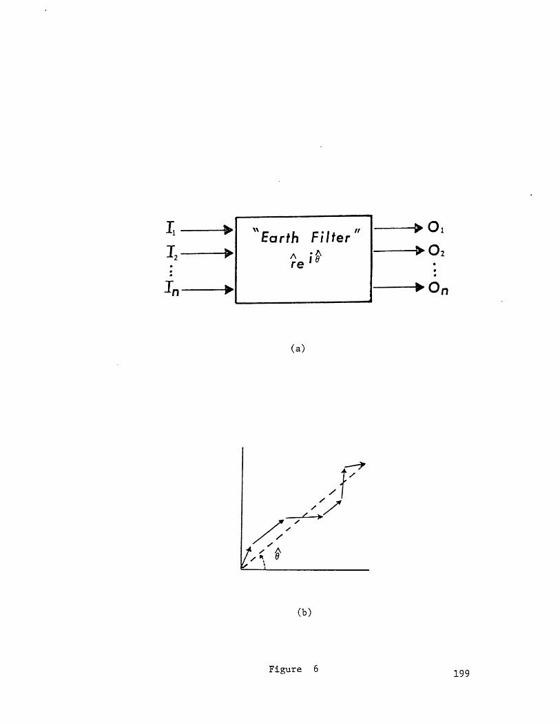
-2

In-

-- 01

0O2

(a)

ot1

(b)

Figure 6 199

Earth FilterAre

Event I

I I I I10 20 30 40 50 60

DEPTH (km)

Oct 1, 1969

(b)

Figure 7

I.0-

0.8.

0.6.

0.4-

0.2-.

(a)

N

1.0

.8-

6--

Event 2

10 20 30 40 50 60

DEPTH (km)

July 24, 1969

(a)(b)

Figure 8

10 20 30 40

DEPTH (km)

May 15, 1976

(a)

Figure 9C)

Event 3

50 60

(b)

Oct 15, 1971

(a)

Event 4

10 20 30 40 50 60DEPTH (kim)

(b)

Figure 10

1.0.

.8-

.6-

.4-4

Event 5

i i i i I

10 20 30 40 50 60

DEPTH (km)

Fe b 14, 1970

(b)

Figure 11

(a)

T= 76 sec

Figure 12

.2.Event 6

10 20 30 40 50 6(

DEPTH ( km)

March 20, 1972

(b)

Figure 13

(a)

1.0...

1.0

0.8

0.6-

0.4.

0.24-

Oct 6, 1976

(a)

Event 7

I I I I I I

20 30 40 50 60

DEPTH (km)

(b)

Figure 14

Station

0- 0

o e0.0

0.

0

WES

00 000 00000000

00* 0 0 0 *00*0.000000

I I I

60 80

T (sec)

Figure .

4.2-

4.0-

E

U

3.8-

3.4-

40

4.2-

4.0+

3 .8

Patton (1978)

0 A AA 0 0 BQ g

jA 0

0

.0

0*

t a

0

Reference Point

9*as0 .4448 .4144*.

. OLoMAAA PDA* VA L+ESK

ESIK

MAL

PTO

ST U

TO L

T R I

VA L

30 50 70 90PERIOD , SEC

(b)

Figure 16

4.2-

4.0-

3.8-

3.6 +

3.4-

T (sec )

(a)

I I I

4.2-

4.0 ... -o- *0 ** * * * *0000000 o0 --o ''o''ooot

/+

4.0

Elbe ric

3 British-- Easter

3 Africco Pacifil

+ Westej

40 60 80

T (sec)

4 .2 - -. 00

0 0 0

~ 4.0 < *) .. 0 00 0O

.000

E* 3.8-- e

.0e 0

3.6-oNA

eT R3.4.R

40 60 80

T (sec)

Figure 18

4.2

4.0---

E 3.8-'' e

3.6e Brazil

Indian

3.4~-- Canadi

40 60 80

T (sec)

Figure

1005

020

Figure

213

4.2

0.S0

0.04.0 000

0

3.8 ' +

E , +o ,' +

3. o -t'0 0

0 , ,'' o RFP- L PA0 0

34-* L P B - C U S (James,1971)- LPB-ARE

- t Tibet

40 60 80

t !

References

Aki, K., Generation and propagation of G waves from the Niigata earthquake of

June 16, 1964, 2, Estimation of earthquake moment, released energy, and

stress-strain drop from G wave spectrum, Bull. Earthquake Res. Inst.

Tokyo, 44, 73-88, 1966.

Aki, K., and H. Patton, Determination of seismic moment tensor using surface

waves, Tectonophys., 49, 213-222, 1978.

Aki, K., and P.G. Richards, Quantitative Seismology, Vol. 2, W.H. Freeman,

San Francisco, 932pp., 1980.

Atwater, T., Implications of plate tectonics for the Cenozoic tectonic

evolution of western North America, Geol. Soc. Amer. Bull, 81, 3513-3536,

1970.

Audebaud, E., R. Capdevilla, B. Dalmayrac, J. Debelmas, G. Laubacher, C.

Lefevre, R. Marocco, C. Martinez, M. Mattauer, F. Megard, J. Paredes, and

P. Tomasi, Les traits geologiques essentiels des Andes Centrales

(Perou-Bolivie), Revue de Geographie Physique et de Geologie Dynamique

(2), 15, 73-114, 1973.

Bally, A.W., P.L. Gordy, and G.A. Stewart, Structure, seismic data and

orogenic evolution of the southern Canadian Rocky Mountains, Bull. Can.

Petr. Geol., 14, 337-381, 1966.

Barazangi, M., and B.L. Isacks, Spatial distribution of earthquakes and

subduction of the Nazca plate beneath South America, Geology, 4, 686-692,

1976.

Barazangi, M., and B.L. Isacks, Subduction of the Nazca plate beneath Peru:

evidence from spatial distribution of earthquakes, Geophys. J.R. astr.

Soc., 57, 537-555, 1979.

215

Brace, W.F., and D.L. Kohlstedt, Limits on lithospheric stress imposed by

laboratory experiments, J. Geophys. Res., 85, 6248-6252, 1980.

Brewer, J.A., S.B. Smithson, J.E. Oliver, S. Kaufman, and L.D. Brown, The

Laramide orogeny: Evidence from COCORP deep crustal seismic profiles in

the Wind River mountains, Wyoming, Tectonophys., 62, 165-189, 1980.

Brune, J.N., Seismic -moment, seismicity, and rate of slip along major fault

zones, J. Geophys. Res., 73, 777-784, 1968.

Brune, J.N., and J. Dorman, Surface waves and earth structure of the Canadian

shield, Bull. Seism. Soc. Amer., 53, 167-210, 1963.

Buland, R., The mechanics of locating earthquakes, Bull. Seism. Soc. Am., 66,

173-187, 1976.

Burchfiel, B.C., and G.A. Davis, Structural framework and evolution of the

southern part of the Cordilleran orogen, western United States, Am. J.

Sci., 272, 97-118, 1972.

Burchfiel, B.C., and G.A. Davis, Nature and controls of Cordilleran

orogenesis, western United States: Extension of an earlier synthesis,

Am. J. Sci., 275-A, 363-396, 1975.

Bussell, M.A., W.S. Pitcher, and P.A. Wilson, Ring complexes of the Peruvian

coastal batholith: a long standing subvolcanic regime, Can. J. Earth

Sci., 13, 1020-1030, 1976.

Chanove, G., M. Mattauer, and F. Megard, Precisions sur la tectonique

tangentielle des terrains secondaries du massif de Pirin (NW du Lac

Titicaca, Perou), C.R. Acad. Sci. Paris, 268, ser D, 1698-1701, 1969.

Chen, W.P., and P. Molnar, Depth distribution of earthquake foci and its

possible implications for the rheological structure of the crust and

upper mantle, (abs.), EOS, 62, 397, 1981.

216

Chen, W.P., and P. Molnar, Seismic moments of major earthquakes and the

average rate of slip in central Asia, J. Geophys. Res., 82, 2945-2969,

1977.

Chinn, P.S., B.L. Isacks, and M. Barazangi, High-frequency seismic wave

propagation in western South America along the continental margin, in the

Nazca plate and across the Altiplano, Geophys. J. Roy. astr. Soc., 60,

204-244, 1980.

Cobbing, E.J., and W.S. Pitcher, The coastal batholith of central Peru, Q.J.

geol. Soc. Lond., 128, 421-460, 1972.

Cobbing, E.J., W.S. Pitcher, and W.P. Taylor, Segments and super-units in the

coastal batholith of Peru, J. Geol., 85, 625-631, 1977.

Coney, P.J., Structural evolution of the Cordillera Huayhuash, Andes of Peru,

Geol. Soc. Am. Bull., 82, 1863-1884, 1971.

Dalmayrac, B., Un example de tectonique vivante: les failles sub-actuelles du

pied de la Cordillera Blanche (Perou), Cah. ORSTOM, Ser. Geol., 6, 19-27,

1974.

Dalmayrac, B., Geologie de la Cordillere orientale de la region de Huanuco: sa

place dans une transversale des Andes du Perou central (9*S a 30*S),

Travaux et Documents de l'ORSTOM, 161 pp., Office de la Recherche

Scientifique et Technique Outre-Mer, Paris, France, 1978.

Dalmayrac, B., and P. Molnar, Parallel thrust and normal faulting in Peru and

constraints on the state of stress, Earth. Plan. Sci. Lett., 55, 473-481,

1981.

Dalmayrac, B., J.R. Lancelot, and A. Leyerloup, Two-billion-year granulites in

the late Precambrian metamorphic basement along the southern Peruvian

coast, Science, 198, 49-51, 1977.

217

Dalmayrac, B., G. Laubacher, and R. Marocco, Geologie des Andes Peruviennes,

Caracteres generaux de l'evolution geologique des Andes peruviennes,

Travaux et Documents de l'ORSTOM, Editions de l'Office de la Recherche

Scientifique et Technique Outre-Mer, Paris, France, 1980.

Davies, G.F., and J.N. Brune, Regional and global fault rates from seismicity,

Nat. Phys. Sci., 229, 101-107, 1971.

Dewey, J.F., and Bird, J.M., Mountain belts and the new global tectonics,

J. Geophys. Res., 75, 2625-2647, 1970.

Deza, E., The Pariahuanca earthquakes, Huancayo, Peru: July-October 1969,

in Recent Crustal Movement, R. Soc. N. Z. Bull., 9, 77-83, 1971.

Dollfus, 0., and F. Megard, Les formations Quaternaires du basin de Huanayo

et leur neotectonique (Andes centrales peruviennes), Rev. Geograph. Phys.

Geol. Dynamique (2), X, 5, 429-440, 1968.

Fitch, T.J., R.G. North, and M.W. Shields, Focal depths and moment tensor

representations of shallow earthquakes associated with the great Sumba

earthquake, J. Geophys. Res., 86, 9357-9374, 1981.

Forsyth, D.W., The early structural evolution and anisotropy of the oceanic

upper mantle, Geophys. J. R. astron. Soc., 43, 103-162, 1975.

Gansser, A., Facts and theories on the Andes, Q.J. geol. Soc. Lon., 129, 93-

131, 1973.

Gee, D.G., Nappe displacement in the Scandinavian Caledonides, Tectonphys.,

47, 393-419, 1978.

Gilbert, F., Excitation of the normal modes of the earth by earthquake

sources, Geophys. J. R. astr. Soc., 22, 223-226, 1970.

Hagiwara, T., A note on the theory of the electromagnetic seismograph,

Bull. Earthquake Res. Inst. Tokyo Univ., 36, 139-164, 1958.

218

Ham, C.K., and L.J. Herrera, Jr., Role of subandean fault system in tectonics

of eastern Peru and Ecuador, in Childs, O.E., and Beebe, R.N., eds.,

Backbone of the Americas, Am. Assoc. Petr. Geol. Mem., 2, 47-61, 1963.

Hamilton, W., The volcanic central Andes - a modern model for the Cretaceous

batholiths and tectonics of western North America, Oregon Dept. Geology

and Mineral Industries, Bull., 65, 175-184, 1969.

Hanks, T.C., and H. Kanamori, A moment magnitude scale, J. Geophys. Res., 84,

2348-2350, 1979.

Harrington, H.J., Paleogeographic development of South America, Bull. Am.

Assoc. Petr. Geol. Bull., 46, 1173-1814, 1962.

Hasegawa, A., and I.S. Sacks, Subduction of the Nazca plate beneath Peru as

determined from seismic observations, J. Geophys. Res., 4971-4980, 1981.

Helwig, J., Plate tectonic model for the evolution of the Central Andes:

Discussion, Geol. Soc. Am. Bull., 84, 1493-1496, 1973.

Hodgson, J.H., and P.C. Bremmer, Direction of faulting in the Ancash, Peru,

earthquake of November 10, 1946, from teleseismic evidence, Seism. Soc.

Am. Bull., 43, 121-125, 1953.

Isacks, B., and P. Molnar, Mantle earthquake mechanism and the sinking of the

lithosphere, Nature, 223, 1121-1124, 1969.

Jackson, J., and T. Fitch, Basement faulting and the focal depth of the larger

earthquakes in the Zagros Mountains (Iran), 64, 561-586, 1981.

James, D., Subduction of the Nazca plate beneath Central Peru, Geology, 7,

174-178, 1978.

James, D.E., Andean crustal and upper mantle structure, J. Geophys. Res., 76,

3246-3271, 1971.

James, D.E., I.S. Sacks, E. Lazo, and 0. Aparicio, On locating local earth-

quakes using small networks, Seis. Soc. Am. Bull., 59, 1201-1212, 1969.

219

Jordan, T.E., B.L. Isacks, R.W. Allmendinger, J.A. Brewer, V.A. Ramos, and

C.J. Ando, Andean tectonics related to geometry of subducted Nazca plate,

submitted to Geol. Soc. Am. Bull., 1982.

Kafka, A.L., and D.J. Weidner, The focal mechanisms and depths of small

earthquakes as determined from Rayleigh wave radiation patterns, Bull.

Seismol. Soc. Am., 69, 1379-1390, 1979.

Kanamori, H., and J.W. Given, Use of long-period surface waves for past

determination of earthquake source parameters, Phys. Earth Planet.

Inter., 27, 8-31, 1981.

Kanamori, H., and G.S. Stewart, Mode of strain release along the Gibbs

fracture zone, Mid-Atlantic ridge, Phys. Earth Planet. Int., 11, 312-332,

1976.

Kanamori, H., and G.S. Stewart, Seismological aspects of the Guatemala

earthquake of February 4, 1976, J. Geophys. Res., 83, 3427-3434, 1978.

Kelleher, J., and W. McCann, Buoyant zones, great earthquakes and unstable

boundaries of subduction, J. Geophys. Res., 81, 4885-4896, 1976.

Klein, F.W., Hypocenter location program HYPOINVERSE, Open-file report 78-694,

United States Geological Survey, Menlo Park, 113pp., 1978.

Kostrov, V.V., Seismic moment and energy of earthquakes, and seismic flow of

rock, Izv. Acad. Sci. USSR, Phys. Solid Earth, 1, 23-44, 1974.

Lanczos, C., Linear Differential Operators, Van-Nostrand Co. Ltd., London,

564pp., 1961.

Landisman, M., Z. Dzeiwonski, and Y. Sato, Recent Improvements in the analysis

of surface wave observations, Geophys. J. R. astron. Soc., 17, 369-403,

1969.

Langston, C.A., A single station fault plane solution, Geophys. Res. Lett., 6,

41-44, 1979.

220

Langston, C.A., and D. Helmberger, A procedure for modeling shallow

dislocation sources, Geophys. J. Roy. Astron. Soc., 42, 117-130, 1975.

Laubacher, G., Geologie de la Cordillera Oriental et de l'Altiplano au Nord

et Nord-ouest du Lac Titicaca, Geologie des Andes Peruviennes, Trauvaux

et Documents de l'ORSTOM, 95 pp., Office de la Recherche Scientifique et

Technique Outre-Mer, Paris, France, 1978.

Lawson, C.L., and R.J. Hanson, Solving Least Squares Problems, Prentice Hall,

Englewood Cliffs, 340pp., 1974.

Lavenu, A. Neotectonique des sediments plio-quaternaires du nord de

l'Altiplano bolivien (Region de La Paz-Ayo-Ayo-Umala), Cah. O.R.S.T.O.M.,

ser. Geol., X, No. 1, 115-126, 1978.

Lavenu, A., and 0. Ballivian, Estudios neotectonicos de las cuencas de las

regiones de Cochabamba, Sucre, Tarija - Cordillera Oriental boliviana,

Rev. Acad. Nac. Cien. Bolivia, 2, No. 3, 107-129, 1979.

Lee, W.H.K., and S.W. Stewart, Principles and Applications of Microearthquake

Networks, Advances in Geophysics, Supplement 2, Academic Press, New York,

1981.

Lepry, L.A., and G.H. Davis, Influence of 'soft' basement on ramp thrusting

in the Yauli dome foreland region, Cordillera Occidental, Peru, submitted

to Geol. Soc. Am. Bull., 1982.

Lilwall, R.C., and T.J.G. Francis, Hypocentral resolution of small ocean

bottom seismic networks, Geophys. J. R. astr. Soc., 54, 721-728, 1978.

Lohman, H.H., Outline of the tectonic history of Bolivian Andes, Am. Assoc.

Petr. Geol. Bull., 54, 735-757, 1970.

McCowan, D.W., Moment tensor representation of surface wave sources, Geophys.

J. R. astron. Soc., 44, 595-599, 1976.

McKenzie, D., Acti-ve tectonics of the Mediterranean region, Geophys. J.R.

astr. Soc., 30, 109-185, 1972.

221

McTigue, D.F., and C.C. Mei, Gravity-induced stresses near topography of small

slope, J. Geophys. Res., 86, 9268-9278, 1981.

Megard, F., Etude geologique des Andes du Perou central, Office de la

Recherche Scientifique et Tecnique Outre-Mer, Mem. 86, 310 pp., 1978.

Megard, F., and H. Philip, Plio-Quaternary Tectono-Magmatic zonation and

plate tectonics in the central Andes, Earth Plan. Sci. Lett., 33, 231-

239, 1976.

Meissner, R., and J. Strehlau, Limits of stresses in continental crusts and

their relation to depth-frequency distribution of shallow earthquakes,

Tectonics, 1, 73-89, 1982.

Mendiguren, J.A., and F.M. Richter, On the origin of compressional intraplate

stresses in South America, Phys. Earth Plan. Int., 16, 318-326, 1978.

Mercier, J.L., Extensional-compressional tectonics associated with the Aegean

Arc: comparison with the Andean Cordillera of south Peru-north Bolivia,

Phil. Trans. R. Soc. Lond., 300, 337-355, 1981.

Molnar, P., Earthquake recurrence intervals and plate tectonics, Bull. Seis.

Soc. Am., 69, 115-133, 1979.

Molnar, P., and P. Tapponnier, Cenozoic tectonics of Asia: effects of a

continental collision, Science, 189, 419-426, 1975.

Molnar, P., and P. Tapponnier, Active tectonics of Tibet, J. Geophys. Res.,

83, 5361-5375, 1978.

Molnar, P., W.P. Chen, T.J. Fitch, P. Tapponnier, W.E.K. Warsi, and F.T. Wu,

Structure and tectonics of the Himalaya; A brief summary of relevant

geophysical observation, in Himalaya: Sciences de la Terre, pp. 269-294,

Centre National de la Recherche Scientifique, Paris, 1977.

Nabelek, J., G. Suarez, and M.N. Toksoz, the 1982 New Brunswick Earthquake:

Inversion of Focal Depth and Source Mechanism from Body and Surface

Waves, in preparation, 1982.

222

Newell, N.D., Geology of the Lake Titicaca region, Peru and Bolivia, Geol.

Soc. Am. Mem., 36, 111 pp., 1949.

Noble, D.C., and E.J. McKee, Spatial distribution of earthquakes and

subduction of the Nazca plate beneath south: Comment, Geology, 5,

576-578, 1977.

Ocola, L.C., and R.P. Meyer, Crustal structure from the Pacific basin to the

Brazilian shield between 120 and 30* south latitude, Bull. Seism. Soc.

Amer., 84, 3387-3403, 1973.

Ocola, L.C., R.P. Meyer, and L.T. Aldrich, Gross crustal structure under Peru-

Bolivia Altiplano, Earthquake Notes, 42, 33-48, 1971.

Paredes, J., Etude geologique de la feuille de Jauja au 1:100,000 (Andes du

Perou Central), These 3eme Cycle, Univ. Sci. Tech. Languedoc,

Montpellier, 79pp., 1972.

Patton, H., Source and Propagation effects of Rayleigh waves from Central

Asian Earthquakes, Ph.D. thesis, 342pp., Mass. Inst. of Technol.,

Cambridge, 1978.

Patton, H., Reference point equalization method for determining the source and

path effects of surface waves, J. Geophys. Res., 85, 821-848, 1980.

Pennington, W.D., Subduction of the Eastern Panama Basin and seismotectonics

of Northwestern South America, 86, 10753-10770, 1981.

Philip, H., and F. Megard, Structural analysis of the superficial deformation

of the 1969 Pariahuanca earthquakes (central Peru), Tectonophys., 38,

259-278, 1977.

Pilger, R.H., Plate reconstructions of aseismic ridges, and low angle

subduction beneath the Andes, Geol. Soc. Am. Bull., 92, 448-456, 1981.

Pilger, R.H. and D.W. Handschumacher, The fixed-hotspot hypothesis and origin

of the Easter-Sala y Gomez-Nazca trace, Geol. Soc. Amer. Bull., 92,

437-446, 1981.

223

Pisarenko, V.F., Statistical estimates of amplitude and phase corrections,

Geophys. J. R. astron. Soc., 20, 89-98, 1970.

Pitcher, W., On the rate of emplacement of batholiths, Q.J. Geol. Soc. Lond.,

581-591, 1975.

Plafker, G., Alaskan earthquake of 1964 and Chilean earthquake of 1960:

implications for arc tectonics, J. Geophys. Res., 77, 901-925, 1972.

Prevot, R., D. Hatzfeld, S.W. Roecker and P. Molnar, Shallow Earthquakes and

Active Tectonics in Eastern Afghanistan, J. Geophys. Res., 85, 1347-1357,

1980.

Price, R.A.,. and E.W. Mountjoy, Geologic structure of the Canadian Rocky

Mountains between Bow and Athabaska Rivers - a progress report, Geol.

Assoc. Canada Spec. Paper, 6, 7-25, 1970.

Rial, J.A., The Caracas, Venezuela, earthquake of July 1967: A multiple-source

event, J. Geophys. Res, 83, 5405-5414, 1978.

Richter, C.F., Elementary Seismology, W.H. Freeman, San Francisco, 768 pp.,

1958.

Rodriguez, A., and A. Chalco, Cuenca Huallaga, Resena geologica y

posibilidades petroliferas, Bol. Soc. Geol. Peru, 49, 187-212, 1975.

Roecker, S.W., Seismicity and Tectonics of the Pamir-hindu Kush region of

Central Asia, Ph.D. thesis, M.I.T., 297 pp., 1981.

Roecker, S.W., 0.V. Soboleva, I.L. Nersesov, A.A. Lukk, D. Hatzfeld,

J.L. Chatelain, and P. Molnar, Seismicity and fault plane solutions

of intermediate depth earthquakes in the Pamir-Hindu Kush region,

J. Geophys. Res., 85, 1358-1364, 1980.

Romanowicz, B., Depth resolution of Earthquakes in Central Asia by Moment

Tensor Inversion of Long-Period Rayleigh Waves: Effects of Phase

Velocity Variations across Eurasia, J. Geophys. Res., 86, 5963-5984,

1981.

224

Romanowicz, B., Moment Tensor Inversion of Long-Period Rayleigh Waves: A New

Approach, J. Geophys. Res., 87, 5395-5407, 1982a.

Romanowicz, B., Constraints on the structure of the Tibet plateau from pure

path phase velocities of Love and Rayleigh waves, J. Geophys. Res., 87,

6865-6883, 1982b.

Saito, M., Excitation of free oscillations and surface waves by a point source

in a vertically heterogeneous earth, J. Geophys. Res., 72, 3689-3699,

1967.

Sales, J.K., Cordilleran foreland deformation, Am. Assoc. Petroleum Geol.

Bull., 52, 2016-2044, 1968.

Sclater, J.G., V. Vacquier, and J.H. Rohrhirsch, Terrestrial heat flow

measurements on Lake Titicaca, Peru, Earth Planet. Sci. Lett., 8, 45-54,

1970.

Shackleton, R.M., A.C. Ries, M.P. Coward, and P.R. Cobbold, Structure,

metamorphism, and geochronology of the Arequippa Massif of coastal Peru,

136, 2, 195-214, 1979.

Silgado, E., The Ancash, Peru, earthquake of November 10, 1946, Bull. Seism.

Soc. Am., 41, 83-100, 1951.

Smithson, S.B., J.A. Brewer, S. Kaufman, J.E. Oliver, and C.A. Hurich,

Structure of the Laramide Wind River uplift, Wyoming, from COCORP deep

reflection data and from gravity data, J. Geophys. Res., 84, 5955-5972,

1979.

Stauder, W., Mechanism and spatial distribution of Chilean earthquakes with

relation to subduction of the oceanic plate, J. Geophys. Res., 78, 5033-

5061, 1973.

Stauder, W., Subduction of the Nazca plate under Peru as evidenced by focal

mechanisms and by seismicity, J. Geophys. Res., 80, 1053-1064, 1975.

225

Stearns, D.W., Faulting and forced folding in the Rocky Mountain foreland,

in Matthews, V., III, ed., Laramide Folding Associated with Basement

Block Faulting in the Western United States, Geol. Soc. Am. Memoir,

151, 1-37, 1978.

Stewart, J.S.W., J.F. Evernden, and N.J. Snelling, Age determinations from

Andean Peru: a reconnaissance survey, Geol. Soc. Am. Bull., 85,

1107-1116, 1974.

Suarez, G., P. Molnar and B.C. Burchfiel, Seismicity, Fault Plane Solutions,

Depth of Faulting, and Active Tectonics of the Central Andes, J. Geophys.

Res., in press, 1983.

Tatel, H.E., and M.A. Tuve, Seismic studies in the Andes, Amer. Geophys.

Union Trans., 39, 580-582, 1958.

Tapponnier, P., and P. Molnar, Active faulting and tectonics in China, J.

Geophys. Res., 82, 1977.

Touzett, G., Evaluacion geologica del yacimiento petrolifero Agua Caliente,

Bol. Soc. Geol. Peru, 48, 9-24, 1975.

Trehu, A.M., Seismicity and Structure of the Orozco Transform Fault from Ocean

Bottom Seismic Observations, Ph.D. Thesis, Mass. Inst. of Technol./Woods

Hole Oceanographic Inst., 370pp., 1982.

Trehu, A.M., J.L. Nabelek, and S.C. Solomon, Source characterization of two

Reykjanes Ridge earthquakes: surface waves and moment tensors; P

waveforms and nonorthogonal nodal planes, J. Geophys. Res., 86,

1701-1724, 1981.

Tsai, Y.-B., and K. Aki, Precise focal depth determination from amplitude

spectra of surface waves, J. Geophys. Res., 75, 5729-5743, 1970.

Vicente, J.C., F. Sequeiros, M.A. Valdivia, and J. Zavala, El sobre-

escurrimiento de Cincha-Lluta: Elemento del accidente mayor andino al NW

de Arequipa, Bol. Soc. Geol. Peru, 61, 67-100, 1979.

226

Vogt, P.R., A. Lowrie, D.R. Bracey, and R.N. Hey, Subduction of aseismic

oceanic ridges: effects on shape, seismicity and other characteristics of

consuming plate boundaries, Geol. Soc. Am. Spec. Paper, 172, 59 pp.,

1976.

Wagner, D., Statistical decision theory applied to the focal mechanism of

Peruvian earthquakes, Ph.D. dissertation, 176 pp., St. Louis Univ., St.

Louis, Mo., 1972.

Weidner, D.L., Rayleigh waves from mid-ocean ridge earthquakes: source and

path effects, Ph.D. thesis, M.I.T., 253 pp., 1972.

Weidner, D.L., and K. Aki, Focal depth and mechanism of mid-ocean ridge

earthquakes, J. Geophys. Res., 86, 1818-18319 1973.

Wesnousky, S.G., C.H. Scholz, and K. Shimazaki, Deformation of an island arc:

Rates of moment-release and crustal shortening in intraplate Japan

determined from seismicity and Quaternary fault data, J. Geophys. Res.,

in press, 1982.

Wilson, J.J., Cretaceous stratigraphy of the central Andes of Peru, Amer.

Assoc. Petr. Geol. Bull., 47, 1-34, 1963.

Wilson, J.J., L. Reyes, and J. Garayar, Geologia de los Cuadrangulos de

Mollebamba, Tayabamba, Huaylas, Pomabamba, Carhuaz y Huari, Servicio de

Geologia y Mineria, Bol. 16, Lima, Peru, 95 pp., 1967.

Yamashina, K., K. Shimazaki, T. Kato, Aseismic belt along the frontal arc

and plate subduction in Japan, J. Phys. Earth, 26, 447-458, 1978.

Yonekura, N., T. Matsuda, M. Nogami, and S. Kaizuka, An active fault along

the western part of the Cordillera Blanca, Peru, J. Geography Tokyo,

88, 1-19, 1979.

Zeil, W., The Andes a geological review, 260 pp., Gebruder Borntraeger,

Berlin-Stuttgart, Germany, 1979.

227

Appendix 1

Fault plane solutions and synthetic waveforms for the

earthquakes listed in Tables 1 and 2. First motion data are

plotted on equal area lower hemispheric projections where

the solid circles indicate compressional first motions and

open circles dilatational first motions. Observed long

period P waves and synthetic waveforms for the fault plane

solutions shown are also presented for a few stations. Not

all the stations used in the analysis are shown since many

of them, specially those in North America and Europe, are

clustered at similar azimuth and epicentral distance from

the source and have very similar waveforms. Synthetic

waveforms computed at various focal dephts are also shown

versus the observed long period P waves at a few stations

spanning a range of azimuths and epicentral distances.

Arrow indicates preferred focal depth. + indicates ampli-

tude was reduced in half for plotting purposes.

228

GEO

Event 15-19-63h=16km

30 s

MAL

h=12km

14

-.. 16

Obs

18

GEO

229

Vrl-.,

Event 211-3-63

NOR

TUC

30s

STU

h=10km

14

16

-- 18

Obs 44K20

24

NOR

'NV

Mx-

'\ff

'yr

TOL L PA

AKU

h=24km

28

--- o-32

Obs

34

36

40

NORLPA RAR

AL-

Avt

AKU+

KIP

h=14km

18

Obs

-20

22

26

h=20km

KIP+ SDB*

SCP

BEC

SHA

BKS

Event 56-20-68

BKS

h=12 km

14

Obs

18

20

22

VAL,/4^%

PTO

NAT

ESK

h=16 km

30s

OGD NAT

233

BECSJG

Event 612-1-68

LPAh=18 km

30s

SJG

ANA

LPA NAT

h=14 km

-18

Obs

22

26

234

WESSHA

DUG

Event 77-24-69

h=6km

30s

h=2km

DUG PTO NAT

BEC

MAL

NAT

WES

A-6 v\

8

Obs

10

14

235

SCP AAM SCP PTO SBA

Event PTO h=lkm10-1-69 k

NAT

JCT 'P

h=5km LPA

12l(PVUa_

GEO SJG

SHA

AA-

MAL

SDB

LPAh=28 km

Event 9

30s 2-9-70

SJG

h=20km

MAL LPA GEO

26

Obs

-- 28 %

30

34

237

Event 1012-10-70 AKU +

h= 24 km

28

Obs

-- 32

36

38

AKU+

KIP +

RAR

ESK

VAL+

h=32km

SPA +

CVK

KIP + SPA+

~fLIlL

SJG

BEC

LUB

h = 4km

SJG

6

Obs

80

12

239

Event 123-20-72 SCP BEC TOL NAT L PA ALQ

DXF~I KGh34km

Ap ~MAL 3

Obs

r, SP L PA42

h=38km

4

30s

ATL

Event 132-23-73h=10km

30s

ALQ NAT OXF BKS

h=6 km

OXF

SCP 8

p10

-t Obs

12NAT

14

16

Event 14 NAT9-27-74

h=6km

30s

NAT

h=2 km

3

5

Obs

6

8 \A

242

SCP

Event154-9-76

MSO

TUC

COL

h=22 km

30 s

GDH

h= 14km

VAL

Obs

- 22

26

PTO GDH COL BLA

BKS+ DAL+ FVM WES TOL

FVM OGD Dh=2kh=12 km

TUC KTG 16

Obs

T01

131

Eve 20

h 4km

30s 24

OGD

h=1Okm

12

14

Obs

18

20

OGD

WES

Event 1710-6-76

h =16 km

30s

Appendix 2

Phase velocities measured from the reference point

to WWSSN stations around the world. Phase velocities are

plotted for different stations grouped by geographical

area.

246

ANDES4.2--

4.0-- " m4 .00 0

U 0

A U

3.8 . A * o GIE

A o LPAuA0

3.6 0 A ANT

SPA

3.4 o SBA

20 .I I |

20 40 60 80

T sec

Brazilian Shield

A *0

* TRN

NAT

-I I I I I I I

60T (sec)

4.2

LI4)

4.0-

3.8-

3.6

3.4

40 80

Scandinavia4.2

4.04li--

E 3.8

A COP

3.6 A KON

o AKUa KEV

34 v UMEe NUR

40 60 80

T sec

4.2

4.0-

3.8

I I I I

40 60

T sec

AFRICA

v*

A NAIo BUL= PREv CRM* WINo SDB

U

E

3.6

3.4-

80

Pacific Stations

VPMGo RAR

A WEL

* KIPo AFI

A TAU

* CTA

40 60

T (sec)

4.2-

4.0-

3.8-

V4)

E

U

3.6-

3.4

80

Eastern North America

4.24-

4.0-

3.8-

A0

00 0 0]

0

00

so

3.6P

3.4-

40

T (sec)

U

E

LI

o SCP

v BEC

e BLA

=GEOo OXF

A WES

60 80

- Western North

y 0

0

0p V

0

o ALQ

JCT

~ TUC

-'III|20 60 80

T sec

4.2

4.0

3.8

3.6

IA

4

E

3.4

I

America

E 3.8-

3.6-*O 3-6-- TOLoMALAPDA

3.4 sVAL+ESK

40 60 80

T (sec)

.I

Period (sec) ADE AFI AKU ALQ ATL BEC BLA

100 4.075 4.082 4.094

96 4.055 4.063 4.081

92 4.029 4.047 4.078

88 4.006 4.034 4.077

84 3.994 4.023 4.070

80 3.982 4.014 4.055

76 3.950 4.005 4.020 3.957

72 3.949 3.992 4.009 3.968 3.995

68 3.992 3.982 4.025 3.952 3.968 4.013

64 3.983 3.972 4.017 3.979 3.952 3.998 3.986

60 3.967 3.963 4.012 3.959 3.940 3.987 3.961

56 3.962 3.965 4.008 3.950 3.930 3.996 3.959

52 3.943 3.952 4.007 3.899 3.918 3.972 3.937

48 3.926 3.953 3.984 3.886 3.894 3.968 3.927

44 3.961 3.953 3.979 3.857 3.888 3.952 3.906

40 3.953 3.947 3.970 3.852 3.864 3.920 3.885

36 3.942 3.947 3.945 3.820 3.833 3.896 3.859

32 3.935 3.949 3.947 3.779 3.792 3.857 3.821

28 3.926 3.948 3.989 3.727 3.726 3.807 3.765

24 3.939 3.941 3.884 3.663 3.648 3.718 3.669

20 3.943 3.923 3.774 3.533 3.586 3.583 3.565

255

Period (sec)

100

96

92

88

84

80

76

72

68

64

60

56

52

48

44

40

36

32

28

24

20

BUL

4.122

4.120

4.129

4.108

4.088

4.077

4.079

4.065

4.059

4.055

4.042

4.038

4.027

4.018

4.005

3.982

3.959

3.930

3.879

3.775

COP

4.111

4.097

4.081

4.066

4.056

4.048

4.041

4.032

4.017

3.997

3.999

4.005

3.997

3.983

3.975

3.960

3.952

3.926

3.891

3.856

CTA

102

084

057

044

029

006

990

954

002

993

974

940

959

951

955

953

951

948

939

935

ESK

133

124

115

105

085

060

058

074

088

087

066

056

046

031

018

003

982

959

929

897

GEO

4.017

4.003

4.015

3.999

3.959

3.970

3.974

3.977

3.962

3.942

3.931

3.903

3.874

3.836

3.770

3.674

GRM

4.082

4.063

4.047

4.034

4.023

4.014

4.005

3.992

3.982

3.972

3.963

3.965

3.952

3.953

3.953

3.947

3.947

3.949

3.948

3.941

JCT

.995

.970

.958

.939

.926

.941

.882

.860

.832

.816

.773

.713

.636

3.668 3.785 3.928 3.794 3.559 3.923 3.565

256

Period (sec) KEV KIP KON MAL NAI NAT NU R

100 4.125 3.905 4.134 4.136

96 4.103 4.060 4.141 4.128

92 4.090 3.907 4.134 4.120

88 4.099 4.042 4.119 4.110

84 4.089 4.024 4.103 4.015 4.134

80 4.066 3.890 4.096 4.100 4.135

76 4.049 3.895 4.101 4.082 4.126

72 4.056 3.893 4.073 4.081 4.065 4.098

68 4.051 4.006 4.059 4.067 4.051 4.082

64 4.029 3.890 4.044 4.072 4.040 4.064

60 4.033 3.988 4.035 4.062 4.044 4.086 4.055

56 4.024 3.889 4.026 4.066 4.030 4.062 4.049

52 4.020 3.970 4.018 4.047 4.048 4.069 4.037

48 4.008 3.894 4.012 4.037 4.017 4.051 4.024

44 4.009 3.961 3.999 4.029 4.013 4.051 4.005

40 3.980 3.955 3.984 4.009 3.994 3.996 3.991

36 3.993 3.901 3.939 3.997 3.985 3.967 3.961

32 3.958 3.954 3.950 3.968 3.943 3.904 3.955

28 3.914 3.951 3.920 3.927 3.889 3.811 3.921

24 3.859 3.946 3.860 3.919 3.795 3.728 3.862

20 3.791 3.925 3.777 3.825 3.676 3.614 3.778

257

Period (sec) OXF PDA PMG PRE PTO RAB RAR

100 4.002 4.113 4.071 4.144 4.139 4.067 4.051

96 3.980 4.094 4.059 4.120 4.122 4.053 4.036

92 3.966 4.076 4.045 4.095 4.108 4.039 4.024

88 3.957 4.060 4.033 4.075 4.104 4.026 4.024

84 3.945 4.069 4.032 4.073 4.102 4.017 4.048

80 3.937 4.089 4.013 4.068 4.091 4.010 4.038

76 3.940 4.067 4.000 4.055 4.078 4.001 3.993

72 3.941 4.039 3.986 4.052 4.072 3.989 3.992

68 3.974 4.011 3.979 4.044 4.074 3.983 3.998

64 3.958 4.019 3.974 4.035 4.069 3.976 3.982

60 3.931 4.023 3.964 4.021 4.064 3.969 3.981

56 3.958 4.008 3.955 4.012 4.055 3.946 3.977

52 3.926 4.004 3.950 4.006 4.046 3.978 3.961

48 3.899 3.998 3.938 4.004 4.035 3.967 3.959

44 3.862 3.992 3.936 3.998 4.019 3.966 3.952

40 3.843 3.973 3.938 3.934 4.014 3.957 3.951

36 3.794 3.958 3.945 3.974 3.997 3.952 3.945

32 3.770 3.937 3.938 3.937 3.971 3.934 3.948

28 3.752 3.910 3.932 3.881 3.938 3.949 3.952

24 3.672 3.851 3.943 3.802 3.891 3.932 3.946

20 3.563 3.770 3.929 3.659 3.787 3.934 3.942

258

Period (sec) RIV SCP SDB SJG TAU TOL TRN

100 4.076 4.079 4.157

96 4.059 4.074 4.139

92 4.042 4.070 4.127

88 4.029 4.068 4.135

84 4.016 4.044 4.120

80 4.000 3.998 4.082 4.011 4.099

76 3.991 3.981 4.098 4.001 4.090

72 3.992 3.975 4.079 3.987 4.094

68 3.983 3.971 4.061 3.972 4.081

64 3.957 3.970 4.058 3.962 4.072

60 3.967 3.981 4.042 3.957 4.063

56 3.978 3.952 4.036 3.948 4.061 4.140

52 3.957 3.946 4.031 3.944 3.939 4.058 4.104

48 3.960 3.933 4.020 3.922 3.935 4.039 4.060

44 3.952 3.919 4.016 3.932 3.933 4.030 4.015

40 3.948 3.903 3.998 3.902 3.932 4.019 3.964

36 3.941 3.869 3.973 3.874 3.933 4.000 3.922

32 3.938 3.828 3.946 3.813 3.933 3.979 3.878

28 3.948 3.762 3.907 3.759 3.941 3.941 3.822

24 3.938 3.670 3.846 3.650 3.938 3.894 3.752

20 3.943 3.577 3.690 3.603 3.942 3.787 3.670

259

Period (sec) TUC UME VAL WEL WES WIN

100 4.226 4.106 4.071 4.113

96 4.154 4.092 4.052 4.094

92 4.134 4.078 4.044 4.073

88 4.109 4.060 4.042 4.054

84 4.089 4.039 4.027 4.047

80 3.995 4.087 4.021 4.017 4.055

76 3.960 4.105 4.016 4.005 4.040

72 3.942 4.089 4.018 3.966 4.022

68 3.929 4.056 4.008 3.998 4.042

64 3.910 4.029 3.999 3.978 3.986 4.022

60 3.879 4.029 3.984 3.964 3.972 4.011

56 3.860 4.037 3.979 3.964 3.987 4.009

52 3.984 4.062 4.027 3.964 3.991 4.011

48 3.866 4.037 4.010 3.959 3.968 3.993

44 3.832 4.024 4.000 3.954 3.945 3.983

40 3.812 4.008 3.989 3.953 3.926 3.968

36 3.785 3.985 3.964 3.951 3.896 3.946

32 3.754 3.962 3.938 3.946 3.862 3.920

28 3.714 3.962 3.899 3.944 3.797 3.870

24 3.664 3.884 3.851 3.936 3.708 3.765

20 3.584 3.790 3.759 3.944 3.585 3.640

260