Embed Size (px)
Citation preview
arX
iv:c
s/06
1006
8v2
[cs
.LO
] 2
2 Fe
b 20
07
Universite Paris XI
Orsay, France
Ph. D. Thesis
Type Theory and Rewriting
Frederic BLANQUI
28 september 2001
Committee:
Mr Thierry COQUAND, referee
Mr Gilles DOWEK, president of the jury
Mr Herman GEUVERS, referee
Mr Jean-Pierre JOUANNAUD, supervisor
Mme Christine PAULIN
Mr Miklos SANTHA

The 19th of March 1998 was an important date for at least two reasons. Thefirst one was personal. The second one was that Jean-Pierre Jouannaud agreed tosupervise my master thesis on “extending the Calculus of Constructions with a newversion of the General Schema” which he had roughed out with Mitsuhiro Okada.This did not mean much to me then. However, I was very happy with the idea ofstudying both λ-calculus and rewriting, and their interaction. This work results ofthis enthusiasm.
This is why I will begin by thanking Jean-Pierre Jouannaud, for the honor hemade to me, the trust, the help, the advice and the support that he gave me duringthese three years. He taught me a lot and I will be always grateful to him.
I also thank Mitsuhiro Okada for the discussions we had together and the supporthe gave me. It was a great honor to have the opportunity to work with him. I hopewe will have other numerous fruitful collaborations.
I also thank Maribel Fernandez who helped me at the beginning of my thesis bysupervising my work with Jean-Pierre Jouannaud.
I also thank Gilles Dowek who supported me in my work and helped me onseveral important occasions. His work was (and still is !) an important source ofreflexion and inspiration.
I also thank Daria Walukiewicz with whom I had many fruitful discussions. Ithank her very much for having read in detail an important part of this thesis andfor having helped me to correct errors and lack of precision.
I also thank every person in the DEMONS team from the LRI and the Coq team(newly baptized LogiCal) from INRIA Rocquencourt, in particular Christine Paulinand Claude Marche who helped me several times. These two teams are a privilegedresearch place and have a pleasant atmosphere.
I also thank the referees of this thesis, Thierry Coquand and Herman Geuvers,for their interest in my work and the remarks they made for improving it.
Finally, I thank the members of the jury and the president of the jury for thehonor they made to me by accepting to consider my work.


Contents
1 Introduction 7
1.1 Some history . . . . . . . . . . . . . . . . . . . . . . . . . . . . . . . 7
1.2 Motivations . . . . . . . . . . . . . . . . . . . . . . . . . . . . . . . . 17
1.3 Previous works . . . . . . . . . . . . . . . . . . . . . . . . . . . . . . 20
1.4 Contributions . . . . . . . . . . . . . . . . . . . . . . . . . . . . . . . 22
1.5 Outline of the thesis . . . . . . . . . . . . . . . . . . . . . . . . . . . 23
2 Preliminaries 25
3 Type Systems Modulo (TSM’s) 29
3.1 Definition . . . . . . . . . . . . . . . . . . . . . . . . . . . . . . . . . 30
3.2 Properties . . . . . . . . . . . . . . . . . . . . . . . . . . . . . . . . . 33
3.3 TSM’s stable by substitution . . . . . . . . . . . . . . . . . . . . . . 35
3.4 Logical TSM’s . . . . . . . . . . . . . . . . . . . . . . . . . . . . . . 37
4 Reduction Type Systems (RTS’s) 41
4.1 Definition . . . . . . . . . . . . . . . . . . . . . . . . . . . . . . . . . 41
4.2 Logical and functional RTS’s . . . . . . . . . . . . . . . . . . . . . . 43
4.3 Logical and injective RTS’s . . . . . . . . . . . . . . . . . . . . . . . 45
4.4 Confluent RTS’s . . . . . . . . . . . . . . . . . . . . . . . . . . . . . 48
5 Algebraic Type Systems (ATS’s) 51
6 Conditions of Strong Normalization 57
6.1 Term classes . . . . . . . . . . . . . . . . . . . . . . . . . . . . . . . . 57
6.2 Inductive types and constructors . . . . . . . . . . . . . . . . . . . . 58
6.3 General Schema . . . . . . . . . . . . . . . . . . . . . . . . . . . . . . 63
6.3.1 Higher-order rewriting . . . . . . . . . . . . . . . . . . . . . . 63
6.3.2 Definition of the schema . . . . . . . . . . . . . . . . . . . . . 65
6.4 Strong normalization conditions . . . . . . . . . . . . . . . . . . . . . 71
7 Examples of CAC’s 77
7.1 Calculus of Inductive Constructions (CIC) . . . . . . . . . . . . . . . 77
7.2 CIC + Rewriting . . . . . . . . . . . . . . . . . . . . . . . . . . . . . 87
7.3 Natural Deduction Modulo (NDM) . . . . . . . . . . . . . . . . . . . 88
5
6
8 Correctness of the conditions 918.1 Terms to be interpreted . . . . . . . . . . . . . . . . . . . . . . . . . 918.2 Reductibility candidates . . . . . . . . . . . . . . . . . . . . . . . . . 938.3 Interpretation schema . . . . . . . . . . . . . . . . . . . . . . . . . . 978.4 Interpretation of constant predicate symbols . . . . . . . . . . . . . . 1028.5 Reductibility ordering . . . . . . . . . . . . . . . . . . . . . . . . . . 1098.6 Interpretation of defined predicate symbols . . . . . . . . . . . . . . 111
8.6.1 Primitive systems . . . . . . . . . . . . . . . . . . . . . . . . 1128.6.2 Positive, small and simple systems . . . . . . . . . . . . . . . 1128.6.3 Recursive, small and simple systems . . . . . . . . . . . . . . 112
8.7 Correctness of the conditions . . . . . . . . . . . . . . . . . . . . . . 113
9 Future directions of research 121
Bibliography 123
Chapter 1
Introduction
What is good programming? Apart from writing programs which are understandableand reusable by other people, above all it is being able to write programs withouterrors. But how do you know whether a program has no error? By proving it. Inother words, to program well requires doing mathematics.
But how do you know whether a proof that a program has no error itself has noerror? By writing a proof which can be checked by a computer. In other words, toprogram well requires doing formal mathematics.
This is the subject of our thesis : defining a formal system in which one canprogram and prove that a program is correct.
However, it is not the case that work is duplicated : programming and proving.In fact, from a proof that a program specification is correct, one can extract an error-free program! This is due to the termination of “cut elimination” in intuitionist logicdiscovered by G. Gentzen in 1933 [57].
More precisely, we will consider a particular class of formal systems, the typesystems. We will study their properties when they are extended with definitions byrewriting. Rewriting is a simple and general computation paradigm based on ruleslike x + 0 → x, that is, if one has an expression of the form x + 0, then one cansimplify it to x.
But for such a system to serve in proving the correctness of programs, one mustmake sure that the system itself is correct, that is, that one cannot prove somethingwhich is false. This is why we will give conditions on the rewriting rules and provethat these conditions indeed ensure the correctness of the system.
First, let us see how type systems appeared, what results are already known andwhat our contributions are (they are summarized in Section 1.4).
1.1 Some history
This section is not intended to provide an absolutely rigorous historical summary.We only want to recall the basic concepts on which our work is based (type theory,
7

8 CHAPTER 1. INTRODUCTION
λ-calculus, etc.) and show how our work takes place in the continuation of previousworks aiming at introducing more programming into logic, or dually, more logic intoprogramming. We will therefore take some freedom with the formalisms used.
The reader familiar with these notions (in particular the Calculus of Construc-tions and the Calculus of Inductive Constructions) can directly go to Section 1.2where we present our motivations for adding rewriting in the Calculus of Construc-tions both at the object-level and at the predicate-level.
Set theory
One of the first formal system enabling one to describe all mathematics was the set
theory of E. Zermelo (1908) later extended by A. Fraenkel (1922). It was followed bythe type theory of A. Whitehead and B. Russell (1911) [120], also called higher-order
logic . These two formal systems were introduced to avoid the inconsistency of theset theory of G. Cantor (1878).
In first-order logic, in which the set theory of E. Zermelo and A. Fraenkel isgenerally expressed, the objects of the discourse are defined from constants andfunction symbols (0,+, . . .). Then, some predicate symbols (∈, . . . ), the logicalconnectors (∨,∧,⇒, . . .) and the universal and existential quantifiers (∀,∃) enableone to express propositions in these objects.
One of the axioms of G. Cantor’s set theory is the Comprehension Axiom whichsays that every proposition defines a set :
(∃x)(∀y) y ∈ x⇔ P (y)
From this axiom, one can express Russell’s paradox (1902). By taking P (x) =x /∈ x, one can define the set R of the x’s which do not belong to themselves. Then,R ∈ R ⇔ R /∈ R and one can deduce that any proposition is true. To avoid thisproblem, E. Zermelo proposed to restrict the Comprehension Axiom as follows :
(∀z)(∃x)(∀y) y ∈ x⇔ y ∈ z ∧ P (y)
that is, one can define by comprehension only subsets of previously well-defined sets.
Type theory
In type theory, instead of restricting the Comprehension Axiom, the idea is to forbidexpressions like x /∈ x or x ∈ x by restricting the application of a predicate to anobject. To this end, one associates to each function symbol and predicate symbol(except ∈) a type as follows :
– to a constant, one associate the type ι,
– to a function symbol taking one argument, one associates the type ι→ ι,
– to a function symbol taking two arguments, one associates the type ι→ ι→ ι,
– . . .
– to a proposition, one associates the type o,
1.1. SOME HISTORY 9
– to a predicate symbol taking one argument, one associates the type ι→ o,
– to a predicate symbol taking two arguments, one associates the type ι→ ι→ o,
– . . .
Then, one can apply a function f taking n arguments to n objects t1, . . . , tn ifthe type of f is ι → . . . → ι → ι and every ti is of type ι. And one can say that nobjects t1, . . . , tn satisfy a predicate symbol P taking n arguments if the type of Pis ι→ . . .→ ι→ o and every ti is of type ι.
Finally, one considers that a set is not an object anymore (that is, an expressionof type ι) but a predicate (an expression of type ι→ o). And, for representing x ∈ E,which means that x satisfies E, one writes Ex (application of E to x). Hence, onecan easily verify that it is not possible to express Russell’s paradox : one cannotwrite xx for representing x ∈ x since then x is both of the type ι → o and of thetype ι which is not allowed. In the following, we write t : τ for saying that t is oftype τ .
Now, to represent natural numbers, there are several possibilities. However it isalways necessary to state an axiom of infinity for ι and to be able to express the setof natural numbers as the smallest set containing zero and stable by incrementation.To this end, one must be able to quantify on sets, that is, on expressions of typeι→ o.
Now, one is not restricted to objects and predicate expressions as describedbefore, but can consider all the expressions that can be formed by applicationswhich respect types :
– The set of the simple types is the smallest set T containing ι, o and σ → τwhenever σ and τ belong to T .
– The set of terms of type τ is the smallest set containing the constants of type τand the applications tu whenever t is a term of type σ → τ and u a term of typeσ.
Finally, one introduces an explicit notation for functions and sets, the λ-abstrac-tion , and considers logical connectors and quantifiers as predicate symbols by givingthem the following respective types : ∨ : o→ o→ o, ∧ : o→ o→ o, ∀τ : (τ → o)→o, . . . For example, if ι denotes the set of natural numbers then one can represent thepredicate “is even” (of type ι→ o) by the expression pair = λx : ι.∃ι(λy : ι.x = 2×y)that we will abbreviate by λx : ι.∃y : ι.x = 2 × y. The language we obtain is calledthe simply-typed λ-calculus λ→.
But what can we say about (pair 2) and ∃y : ι.2 = 2× y ? The second expressioncan be obtained from the first one by substituting x by 2 in the body of pair. Thisoperation of substitution is called β-reduction . More generally, λx : τ. t applied tou β-reduces to t where x is substituted by u : λx :τ. t u→β t{x 7→ u}.
It is quite natural to consider theses two expressions as denoting the same propo-sition. This is why one adds the following Conversion Axiom :
P ⇔ Q if P →β Q
10 CHAPTER 1. INTRODUCTION
One then gets the type theory of A. Church (1940) [30].
In this theory, it is possible to quantify over all propositions : ∀P : o.P ⇒ P .In other words, a proposition can be defined by quantifying over all propositions,including itself. If one allows such quantifications, the theory is said to be impred-
icative , otherwise it said predicative .
Mathematics as a programming language
The β-reduction corresponds to the evaluation process of a function. When one hasa function f defined by an expression f(x) and wants its value on 5 for example,one substitutes x by 5 in f(x) and simplify the expression until one gets the valueof f(5).
One can wonder which functions are definable in Church’s type theory. In fact,very few. With Peano’s natural numbers (i.e. by taking 0 : ι for zero and s : ι→ ι forthe successor function), one can express only constant functions or functions addinga constant to one of its arguments. With Church’s numerals, where n is representedby λx : ι.λf : ι→ ι.f . . . fx with n occurrences of f , H. Schwichtenberg [105] provedthat one can express only extended polynomials (smallest set of functions closedunder composition and containing the null function, the successor function, theprojections, the addition, the multiplication and the test for zero).
Of course, it is possible to prove the existence of numerous functions, that is,to prove a proposition of the form (∀x)(∃y)Pxy where P represents the graph ofthe function. In the intuitionist type theory for example (i.e. without using theExcluded-middle Axiom P∨¬P ), it is possible to prove the existence of any primitiverecursive function. But there is no term f : ι→ ι enabling us to compute the powersof 2 for example, that is, such that fn→β . . .→β 2n.
Representation of proofs
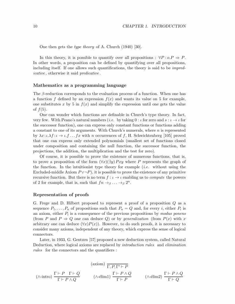
G. Frege and D. Hilbert proposed to represent a proof of a proposition Q as asequence P1, . . . , Pn of propositions such that Pn = Q and, for every i, either Pi isan axiom, either Pi is a consequence of the previous propositions by modus ponens
(from P and P ⇒ Q one can deduce Q) or by generalization (from P (x) with xarbitrary one can deduce (∀x)P (x)). However, to do such proofs, it is necessary toconsider many axioms, independent of any theory, which express the sense of logicalconnectors.
Later, in 1933, G. Gentzen [57] proposed a new deduction system, called NaturalDeduction, where logical axioms are replaced by introduction rules and elimination
rules for the connectors and the quantifiers :
(axiom)Γ, P,Γ′ ⊢ P
(∧-intro)Γ ⊢ P Γ ⊢ Q
Γ ⊢ P ∧Q(∧-elim1)
Γ ⊢ P ∧Q
Γ ⊢ P(∧-elim2)
Γ ⊢ P ∧Q
Γ ⊢ Q

1.1. SOME HISTORY 11
(⇒-intro)Γ, P ⊢ Q
Γ ⊢ P ⇒ Q(⇒-elim)
Γ ⊢ P ⇒ Q Γ ⊢ P
Γ ⊢ Q
(∃-intro)Γ ⊢ P (t)
Γ ⊢ (∃x)P (x)(∃-elim)1
Γ ⊢ (∃x)P Γ, P ⊢ Q
Γ ⊢ Q. . .
where Γ is a set of propositions (the hypothesis). A pair Γ ⊢ Q made of a set ofhypothesis Γ and a proposition Q is called a sequent . Then, a proof of a sequentΓ ⊢ Q is a tree whose root is Γ ⊢ Q, whose nodes are instances of the deductionrules and whose leaves are applications of the rule (axiom).
Cut elimination
G. Gentzen remarked that some proofs can be simplified. For example, this proofof Q :
Γ, P ⊢ Q(⇒-intro)
Γ ⊢ P ⇒ Q Γ ⊢ P(⇒-elim)
Γ ⊢ Q
does a detour which can be eliminated. It suffices to replace in the proof of Γ, P ⊢ Qall the leaves (axiom) giving Γ, P,Γ′ ⊢ P (Γ′ are additional hypothesis that maybe introduced for proving Q) by the proof of Γ ⊢ P where Γ is also replaced byΓ,Γ′. In fact, at every place where there is a cut , that is, an introduction rulefollowed by an elimination rule for the same connector, it is possible to simplifythe proof. G. Gentzen proved the following remarkable fact : the cut-eliminationprocess terminates.
Hence, any provable proposition has a cut-free proof. But, in intuitionist logic,any cut-free proof of a proposition (∃x)P (x) must terminate by an introduction rulewhose premise is of the form P (t). Therefore, the cut-elimination process gives us awitness t of an existential proposition. In other words, any function whose existenceis provable is computable.
If one can express the proofs themselves as objects of the theory, then it becomespossible to express many more functions than those allowed in the simply-typed λ-calculus.
The isomorphism of Curry-de Bruijn-Howard
In 1958, Curry [41] remarked that there is a correspondence between the types ofthe simply-typed λ-calculus and the propositions formed from the implication ⇒(one can identify → and ⇒), and also between the terms of type τ and the proofsof the proposition corresponding to τ . In other words, the simply-typed λ-calculusenables one to represent the proofs of the minimal propositional logic. To this end,one associates to each proposition P a variable xP of type P . Then, one defines theλ-term associated to a proof by induction on the size of the proof :
1If x does not occur neither in Γ nor in Q.
12 CHAPTER 1. INTRODUCTION
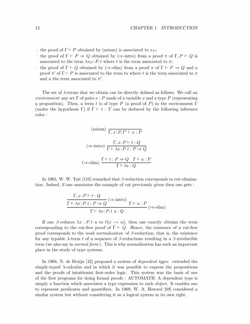
– the proof of Γ ⊢ P obtained by (axiom) is associated to xP ;
– the proof of Γ ⊢ P ⇒ Q obtained by (⇒-intro) from a proof π of Γ, P ⊢ Q isassociated to the term λxP :P. t where t is the term associated to π;
– the proof of Γ ⊢ Q obtained by (⇒-elim) from a proof π of Γ ⊢ P ⇒ Q and aproof π′ of Γ ⊢ P is associated to the term tu where t is the term associated to πand u the term associated to π′.
The set of λ-terms that we obtain can be directly defined as follows. We call anenvironment any set Γ of pairs x : P made of a variable x and a type P (representinga proposition). Then, a term t is of type P (a proof of P ) in the environment Γ(under the hypothesis Γ) if Γ ⊢ t : T can be deduced by the following inferencerules :
(axiom)Γ, x :P,Γ′ ⊢ x : P
(⇒-intro)Γ, x :P ⊢ t : Q
Γ ⊢ λx :P. t : P ⇒ Q
(⇒-elim)Γ ⊢ t : P ⇒ Q Γ ⊢ u : P
Γ ⊢ tu : Q
In 1965, W. W. Tait [110] remarked that β-reduction corresponds to cut-elimina-tion. Indeed, if one annotates the example of cut previously given then one gets :
Γ, x :P ⊢ t : Q(⇒-intro)
Γ ⊢ λx :P. t : P ⇒ Q Γ ⊢ u : P(⇒-elim)
Γ ⊢ λx :P. t u : Q
If one β-reduces λx : P. t u to t{x 7→ u}, then one exactly obtains the termcorresponding to the cut-free proof of Γ ⊢ Q. Hence, the existence of a cut-freeproof corresponds to the weak normalization of β-reduction, that is, the existencefor any typable λ-term t of a sequence of β-reductions resulting in a β-irreducibleterm (we also say in normal form ). This is why normalization has such an importantplace in the study of type systems.
In 1968, N. de Bruijn [42] proposed a system of dependent types extended thesimply-typed λ-calculus and in which it was possible to express the propositionsand the proofs of intuitionist first-order logic. This system was the basis of oneof the first programs for doing formal proofs : AUTOMATH. A dependent type issimply a function which associates a type expression to each object. It enables oneto represent predicates and quantifiers. In 1969, W. A. Howard [69] considered asimilar system but without considering it as a logical system in its own right.

1.1. SOME HISTORY 13
In a dependent type system, the well-formedness of types depends on the well-formedness of terms. It is then necessary to consider environments with type vari-ables and to add typing rules for types and environments (the order of variables nowmatters). Finally, it is necessary to add a conversion rule for identifying β-equivalentpropositions. One then gets a set of typing rules similar to the ones of Figure 1.1(this is a modern presentation which emerged at the end of the 80’s only).centering
Figure 1.1: Typing rules of λP
(ax)⊢ ⋆ : ✷
(var)Γ ⊢ T : s ∈ {⋆,✷}
Γ, x :T ⊢ x : T
(weak)Γ ⊢ t : T Γ ⊢ U : s ∈ {⋆,✷}
Γ, x :U ⊢ t : T
(prod-λ→)Γ ⊢ T : ⋆ Γ, x :T ⊢ U : ⋆
Γ ⊢ (x :T )U : ⋆
(prod-λP )Γ ⊢ T : ⋆ Γ, x :T ⊢ U : ✷
Γ ⊢ (x :T )U : ✷
(abs)Γ, x :T ⊢ u : U Γ ⊢ (x :T )U : s ∈ {⋆,✷}
Γ ⊢ λx :T. u : (x :T )U
(app)Γ ⊢ t : (x :U)V Γ ⊢ u : U
Γ ⊢ tu : V {x 7→ u}
(conv)Γ ⊢ t : T T ↔∗
β T′ Γ ⊢ T ′ : ⋆
Γ ⊢ t : T ′
In this system, ⋆ is the type of propositions and of the sets of the discourse(natural numbers, etc.), and ✷ is the type of predicate types (of which ⋆ is). Forexample, the set of natural numbers nat has the type ⋆, the predicate even hasthe type (n : nat)⋆ that we abbreviate by nat → ⋆ since n does not occur in ⋆(non-dependent product) and nat → ⋆ has the type ✷. Starting from the rule(ax), the rules (var) and (weak) enables one to build environments. The rule (prod-λ→) enables one to build propositions and the rule (prod-λP) enables one to buildpredicate types. In the case of a proposition, if the product is not dependent (x doesnot occur in U) then it is an implication, otherwise it is a universal quantification.In other words, without the rule (prod-λP), we get the simply-typed λ-calculus.The rule (abs) enables one to build a function (if s = ⋆) or a predicate (if s = ✷).Finally, the rule (app) enables the application of a function or a predicate to an
14 CHAPTER 1. INTRODUCTION
argument. In other words, the rules (abs) and (app) generalize the rules (⇒-intro)and (⇒-elim) of the simply-typed λ-calculus.
From the point of view of programming, dependent types enables one to havemore information about data and hence to reduce the risk of error. For example,one can define the type (list n) of lists of natural numbers of length n by declaringlist : nat → ⋆. Then, the empty list nil has the (list 0) and the function conswhich adds a natural number x at the head of a list ℓ of length n has the typenat→ (n :nat)(list n) → (list (s n)). One can then verify if a list does not exceedsome given length.
Inductive definitions
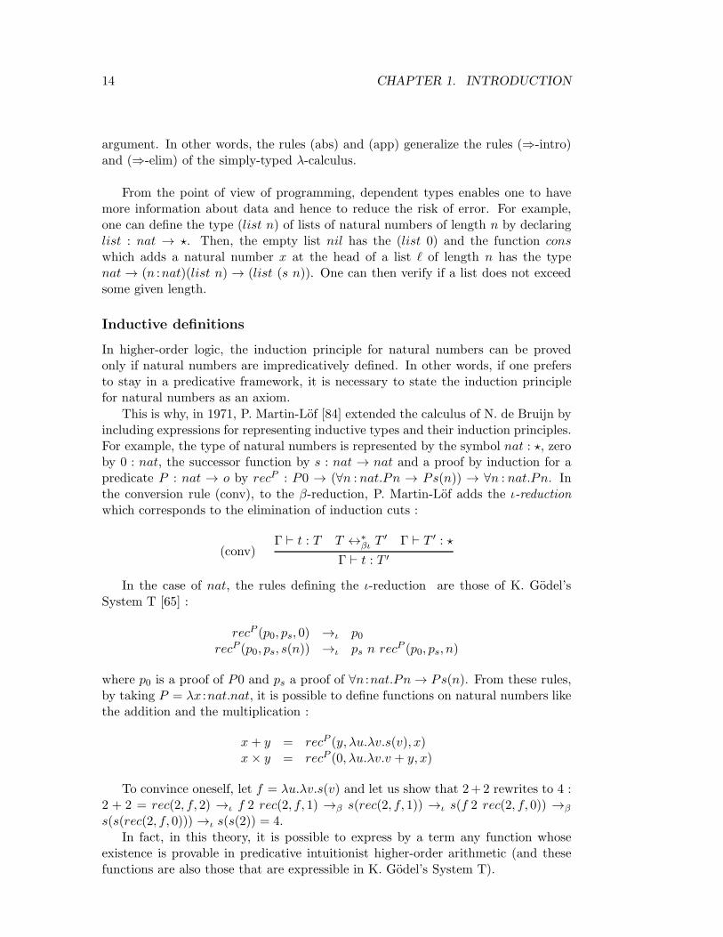
In higher-order logic, the induction principle for natural numbers can be provedonly if natural numbers are impredicatively defined. In other words, if one prefersto stay in a predicative framework, it is necessary to state the induction principlefor natural numbers as an axiom.
This is why, in 1971, P. Martin-Lof [84] extended the calculus of N. de Bruijn byincluding expressions for representing inductive types and their induction principles.For example, the type of natural numbers is represented by the symbol nat : ⋆, zeroby 0 : nat, the successor function by s : nat → nat and a proof by induction for apredicate P : nat → o by recP : P0 → (∀n : nat.Pn → Ps(n)) → ∀n : nat.Pn. Inthe conversion rule (conv), to the β-reduction, P. Martin-Lof adds the ι-reductionwhich corresponds to the elimination of induction cuts :
(conv)Γ ⊢ t : T T ↔∗
βι T′ Γ ⊢ T ′ : ⋆
Γ ⊢ t : T ′
In the case of nat, the rules defining the ι-reduction are those of K. Godel’sSystem T [65] :
recP (p0, ps, 0) →ι p0recP (p0, ps, s(n)) →ι ps n rec
P (p0, ps, n)
where p0 is a proof of P0 and ps a proof of ∀n :nat.Pn→ Ps(n). From these rules,by taking P = λx :nat.nat, it is possible to define functions on natural numbers likethe addition and the multiplication :
x+ y = recP (y, λu.λv.s(v), x)x× y = recP (0, λu.λv.v + y, x)
To convince oneself, let f = λu.λv.s(v) and let us show that 2+ 2 rewrites to 4 :2 + 2 = rec(2, f, 2) →ι f 2 rec(2, f, 1) →β s(rec(2, f, 1)) →ι s(f 2 rec(2, f, 0)) →β
s(s(rec(2, f, 0))) →ι s(s(2)) = 4.
In fact, in this theory, it is possible to express by a term any function whoseexistence is provable in predicative intuitionist higher-order arithmetic (and thesefunctions are also those that are expressible in K. Godel’s System T).
1.1. SOME HISTORY 15
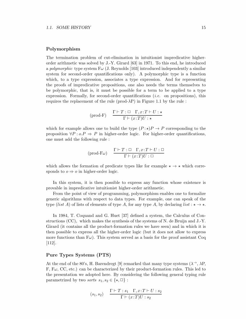
Polymorphism
The termination problem of cut-elimination in intuitionist impredicative higher-order arithmetic was solved by J.-Y. Girard [63] in 1971. To this end, he introduceda polymorphic type system Fω (J. Reynolds [103] introduced independently a similarsystem for second-order quantifications only). A polymorphic type is a functionwhich, to a type expression, associates a type expression. And for representingthe proofs of impredicative propositions, one also needs the terms themselves tobe polymorphic, that is, it must be possible for a term to be applied to a typeexpression. Formally, for second-order quantifications (i.e. on propositions), thisrequires the replacement of the rule (prod-λP) in Figure 1.1 by the rule :
(prod-F)Γ ⊢ T : ✷ Γ, x :T ⊢ U : ⋆
Γ ⊢ (x :T )U : ⋆
which for example allows one to build the type (P : ⋆)P → P corresponding to theproposition ∀P : o.P ⇒ P in higher-order logic. For higher-order quantifications,one must add the following rule :
(prod-Fω)Γ ⊢ T : ✷ Γ, x :T ⊢ U : ✷
Γ ⊢ (x :T )U : ✷
which allows the formation of predicate types like for example ⋆ → ⋆ which corre-sponds to o⇒ o in higher-order logic.
In this system, it is then possible to express any function whose existence isprovable in impredicative intuitionist higher-order arithmetic.
From the point of view of programming, polymorphism enables one to formalizegeneric algorithms with respect to data types. For example, one can speak of thetype (list A) of lists of elements of type A, for any type A, by declaring list : ⋆→ ⋆.
In 1984, T. Coquand and G. Huet [37] defined a system, the Calculus of Con-structions (CC), which makes the synthesis of the systems of N. de Bruijn and J.-Y.Girard (it contains all the product-formation rules we have seen) and in which it isthen possible to express all the higher-order logic (but it does not allow to expressmore functions than Fω). This system served as a basis for the proof assistant Coq[112].
Pure Types Systems (PTS)
At the end of the 80’s, H. Barendregt [9] remarked that many type systems (λ→, λP,F, Fω, CC, etc.) can be characterized by their product-formation rules. This led tothe presentation we adopted here. By considering the following general typing ruleparametrized by two sorts s1, s2 ∈ {⋆,✷} :
(s1, s2)Γ ⊢ T : s1 Γ, x :T ⊢ U : s2
Γ ⊢ (x :T )U : s2
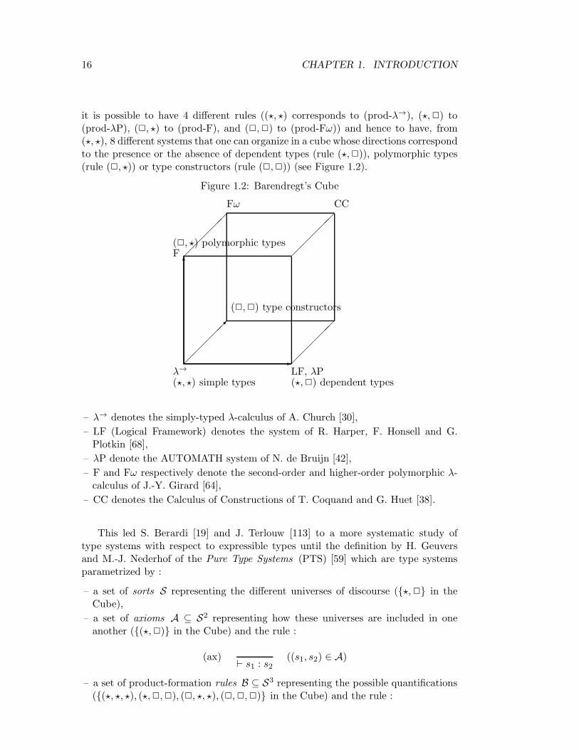
16 CHAPTER 1. INTRODUCTION
it is possible to have 4 different rules ((⋆, ⋆) corresponds to (prod-λ→), (⋆,✷) to(prod-λP), (✷, ⋆) to (prod-F), and (✷,✷) to (prod-Fω)) and hence to have, from(⋆, ⋆), 8 different systems that one can organize in a cube whose directions correspondto the presence or the absence of dependent types (rule (⋆,✷)), polymorphic types(rule (✷, ⋆)) or type constructors (rule (✷,✷)) (see Figure 1.2).
Figure 1.2: Barendregt’s Cube
�����
�����
�����
�����✒
✻
✲λ→
(⋆, ⋆) simple typesLF, λP(⋆,✷) dependent types
(✷,✷) type constructors
(✷, ⋆) polymorphic typesF
Fω CC
– λ→ denotes the simply-typed λ-calculus of A. Church [30],
– LF (Logical Framework) denotes the system of R. Harper, F. Honsell and G.Plotkin [68],
– λP denote the AUTOMATH system of N. de Bruijn [42],
– F and Fω respectively denote the second-order and higher-order polymorphic λ-calculus of J.-Y. Girard [64],
– CC denotes the Calculus of Constructions of T. Coquand and G. Huet [38].
This led S. Berardi [19] and J. Terlouw [113] to a more systematic study oftype systems with respect to expressible types until the definition by H. Geuversand M.-J. Nederhof of the Pure Type Systems (PTS) [59] which are type systemsparametrized by :
– a set of sorts S representing the different universes of discourse ({⋆,✷} in theCube),
– a set of axioms A ⊆ S2 representing how these universes are included in oneanother ({(⋆,✷)} in the Cube) and the rule :
(ax)⊢ s1 : s2
((s1, s2) ∈ A)
– a set of product-formation rules B ⊆ S3 representing the possible quantifications({(⋆, ⋆, ⋆), (⋆,✷,✷), (✷, ⋆, ⋆), (✷,✷,✷)} in the Cube) and the rule :
1.2. MOTIVATIONS 17
(prod)Γ ⊢ T : s1 Γ, x :T ⊢ U : s2
Γ ⊢ (x :T )U : s3((s1, s2, s3) ∈ B)
Calculus of Inductive Constructions (CIC)
We have seen that the Calculus of Constructions is a very powerful system in which itis possible to express many functions. However, these functions cannot be defined asone would like. For example, it does not seem possible to program the predecessorfunction on natural numbers such that its evaluation takes a constant time [64].This is not the case in P. Martin-Lof’s system where natural numbers and theirinduction principle are first-class objects while, in the Calculus of Constructions,natural numbers are impredicatively defined.
This is why, in 1988, T. Coquand and C. Paulin proposed the Calculus of In-ductive Constructions (CIC) [39] which makes the synthesis between the Calculusof Constructions and P. Martin-Lof’s type theory, and hence enable one to writemore efficient programs. In 1994, B. Werner [119] proved the termination of cut-elimination in this system. (In 1993, T. Altenkirch [2] proved also this property butfor a presentation of the calculus with equality judgments.)
But, even in this system, some algorithms may be inexpressible. L. Colson [32]proved for example that, if one uses a call-by-value evaluation strategy (reductionof the arguments first) then the minimum function of two natural numbers cannotbe implemented by a program whose evaluation time is relative to the minimum ofthe two arguments.
1.2 Motivations
We said at the beginning that rewriting is a simple and general computation para-digm based on rewrite rules . This notion is of course very old but it was seriouslystudied from the 70’s with the works of D. Knuth and D. Bendix [18]. They studiedrewriting for knowing whether, in a given equational theory, an equation is valid ornot. Then, rewriting was quickly used as a programming paradigm [96, 67, 55, 71, 31]since any computable function can be defined by rewrite rules (Turing-completeness).
Let us see the case of addition and multiplication on natural numbers definedfrom 0 for zero and s for the successor function :
0 + x → xs(x) + y → s(x+ y)
0× x → 0s(x)× y → (x× y) + y
These rules completely define these two arithmetic operations : starting fromtwo arbitrary natural numbers p and q (expressed with 0 and s), p + q and p × qrewrite in a finite number of steps to a term which cannot be further rewritten, thatis, to a number representing the value of p+ q and p× q respectively.

18 CHAPTER 1. INTRODUCTION
Higher-order rewriting
We can also imagine definitions using functional parameters or abstractions : thisis higher-order rewriting as opposed to first-order rewriting which does not allowfunctional parameters or abstractions. For example, the function map which to afunction f and a list of natural numbers (a1, . . . , an) associates the list (f(a1), . . .,f(an)), can be defined by the following rules :
map(f, nil) → nilmap(f, cons(x, ℓ)) → cons(fx,map(f, ℓ))
where nil stand for the empty list and cons for the function which adds an elementat the head of a list.
Hence, the rules defining the recursor of an inductive type (the ι-reduction) area particular case of higher-order rewriting.
Easier definitions
One can see that definitions by rewriting are more natural and easier to writethan the ones based on recursors like in P. Martin-Lof type theory or in the Calculusof Inductive Constructions. For example, the definition by recursion of the function≤ on natural numbers requires two levels of recursion :
λx.rec(x, λy.true, λnzy.rec(y, false, λn′z′.zn′, y))
while the definition by rewriting is :
0 ≤ y → trues(x) ≤ 0 → false
s(x) ≤ s(y) → x ≤ y
More efficient definitions
From a computing point of view, definitions by rewriting can be made moreefficient by adding rules. For example, with a definition by recursion on its firstargument, n+0 requires n+1 reduction steps. By simply adding the rule x+0→ x,this takes only one step.
However, it can become more difficult to ensure that, for any sequence of argu-ments, the definition always leads, in a finite number of steps (property calledstrongnormalization ), to a unique result (property called confluence ) that we call thenormal form of the starting expression.
Quotient types
Until now we have always spoken of natural numbers but never of integers.Yet they have an important place in mathematics. One way to represent integersis to add a predecessor function p beside 0 and s. Hence, p(p(0)) represents −2.Unfortunately, in this case, an integer can have several representations : p(s(0))or s(p(0)) represent both 0. In fact, integers are equivalent modulo the equationsp(s(x)) = x and s(p(x)) = x.

1.2. MOTIVATIONS 19
However, it is possible to orient these equations so as to have a confluent andstrongly normalizing rewrite system : p(s(x)) → x and s(p(x)) → x. Then, eachinteger has a unique normal form. Therefore, we see that rewriting enables us tomodels quotient types without using further extensions [14].
More typable termsThe introduction of rewriting in a dependent type system allows one to type
more terms and therefore to formalize more propositions. Let us consider, in theCalculus of Inductive Constructions, the type listn : nat → ⋆ of lists of naturalnumbers of length n with the constructors niln : listn(0) for the empty list andconsn : nat → (n : nat)listn(n) → listn(s(n)) for adding an element at the headof a list. Let appn : (n : nat)listn(n) → (n′ : nat)listn(n′) → listn(n + n′) be theconcatenation function. Like +, appn can be defined by using the recursor associatedto the type listn. Assume furthermore that + and appn are defined by inductionon their first argument. Then, the following propositions are not typable :
appn(n, ℓ, 0, ℓ′) = ℓappn(n+ n′, appn(n, ℓ, n′, ℓ′), n′′, ℓ′′) = appn(n, ℓ, n′ + n′′, appn(n′, ℓ′, n′′, ℓ′′))
In the first rule, the left hand-side is of type listn(n+0) and the right hand-sideis of type listn(n). We can prove that (n : nat)n + 0 = n by induction on n butn+0 is not βι-convertible to n since + is defined by induction on its first argument.Therefore, we cannot apply the (conv) rule for typing the equality.
In the second rule, the left hand-side is of type listn((n + n′) + n′′) and theright hand-side is of type listn(n + (n′ + n′′)). Again, although we can prove that(n+n′)+n′′ = n+(n′+n′′) (associativity of +), the two terms are not βι-convertible.Therefore, we cannot apply the (conv) rule for typing the equality.
This shows some limitation of the definitions by recursion. The use of rewriting,that is, the replacement in the (conv) rule of the ι-reduction by a reduction relation→R generated from a user-defined set R of arbitrary rewrite rules :
(conv)Γ ⊢ t : T T ↔∗
βR T ′ Γ ⊢ T ′ : ⋆
Γ ⊢ t : T ′,
allows us to type the previous propositions which are not typable in the Calculus ofInductive Constructions.
Automatic equational proofsAnother motivation for introducing rewriting in type systems is that it makes
equational proofs much easier, which is the reason why rewriting was studied initially.Indeed, in the case of a confluent and strongly normalizing rewrite system, to checkwhether two terms are equal, it suffices to check whether they have the same normalform.
Moreover, it is not necessary to keep a trace of the rewriting steps since thiscomputation can be done again (if the equality is decidable). This reduces the sizeof proof-terms and enable us to deal with bigger proofs, which is a critical problemnow in proof assistants.

20 CHAPTER 1. INTRODUCTION
Integration of decision proceduresOne can also imagine defining predicates by rewriting or having simplification
rules on propositions, hence generalizing the definitions by strong elimination ofthe Calculus of Inductive Constructions [99]. For example, one can consider the setof rules of Figure 1.3 [70] where xor (exclusive “or”) and ∧ are commutative andassociative symbols, ⊥ represents the proposition always false and ⊤ the propositionalways true (by taking a constant I of type ⊤).
Figure 1.3: Decision procedure for classical propositional tautologies
P xor⊥ → PP xorP → ⊥
P ∧⊤ → PP ∧⊥ → ⊥P ∧ P → P
P ∧ (Q xorR) → (P ∧Q) xor (P ∧R)
¬P → P xor⊤P ∨Q → (P ∧Q) xorP xorQP ⇒ Q → (P ∧Q) xorP xor⊤P ⇔ Q → (P xorQ) xor⊤
J. Hsiang [70] showed that this system is confluent and strongly normalizing andthat a proposition P is a tautology (i.e. is always true) if P reduces to ⊤. Thissystem is therefore a decision procedure for classical propositional tautologies.
Hence, type-level rewriting allows the integration of decision procedures. Indeed,thanks to the conversion rule (conv), if P is a tautology then I, the canonical proofof ⊤, is a proof of P . In other words, if the typing relation is decidable, to knowwhether a proposition P is a tautology, it is sufficient to propose I to the verificationprogram.
We can also imagine simplification rules for equality like the ones of Figure 1.4where + and × are associative and commutative, and = is commutative.
Figure 1.4: Simplification rules for equality
x+ 0 → xx+ s(y) → s(x+ y)x× 0 → 0
x× s(y) → (x× y) + xx× (y + z) → (x× y) + (x× z)
x = x → ⊤s(x) = s(y) → x = ys(x) = 0 → ⊥x+ y = 0 → x = 0 ∧ y = 0x× y = 0 → x = 0 ∨ y = 0
1.3 Previous works
The first works on the combination of typed λ-calculus and (first-order) rewritingwere due to V. Breazu-Tannen in 1988 [25]. They showed that the combinationof simply-typed λ-calculus and first-order rewriting is confluent if the rewriting isconfluent. In 1989, V. Breazu-Tannen and J. Gallier [26], and M. Okada [97] in-dependently, showed that the strong normalization is also preserved. These resultswere extended by D. Dougherty [47] to any “stable” set of pure λ-terms.
1.3. PREVIOUS WORKS 21
In 1991, J.-P. Jouannaud and M. Okada [74] extended the result of V. Breazu-Tannen and J. Gallier to higher-order rewrite systems satisfying the General Sche-
ma , a generalization of the primitive recursion schema. With higher-order rewriting,strong normalization becomes more difficult to prove since there is a strong inter-action between rewriting and β-reduction, which is not the case with first-orderrewriting.
In 1993, M. Fernandez [54] extended this method to the Calculus of Constructionswith object level rewriting and simply typed symbols. The methods used for first-order rewriting and non dependent systems [26, 47] cannot be applied to this casesince rewriting is not just a syntactic addition : since rewriting is included in thetype conversion rule (conv), it is a component of typing (in particular, it allows moreterms to be typed).
Other methods for proving strong normalization appeared. In 1996, J. van de Pol[116] extended to the simply-typed λ-calculus the use of monotone interpretations.In 1999, J.-P. Jouannaud and A. Rubio [76] extended to the simply-typed λ-calculusthe method RPO (Recursive Path Ordering) [100, 44]. This method (HORPO) ismore powerful than the General Schema since it is a recursively defined ordering.
In all these works, even the ones on the Calculus of Constructions, functionsymbols are always simply typed. It was T. Coquand [34] in 1992 who initiated thestudy of rewriting on dependent and polymorphic symbols. He studied the complete-ness of definitions on dependent types. For the strong normalization, he proposeda schema more general than the schema of J.-P. Jouannaud and M. Okada since itallows recursive definitions on strictly positive types [39] but it does not necessaryimply strong normalization. In 1996, E. Gimenez [62] defined a restriction of thisschema for which he proved strong normalization. In 1999, J.-P. Jouannaud, M.Okada and I [23, 22] extended the General Schema, keeping simply typed symbols,in order to deal with strictly positive types. Finally, in 2000, D. Walukiewicz [118]extended J.-P. Jouannaud and A. Rubio’s HORPO to the Calculus of Constructionswith dependent and polymorphic symbols.
But there still is a common point between all these works : rewriting is alwaysconfined to the object level.
In 1998, G. Dowek, T. Hardin and C. Kirchner [50] proposed a new approach todeduction for first-order logic : the Natural Deduction Modulo (NDM) a congruence≡ on propositions. This deduction system consists of replacing the rules of usualNatural Deduction by rules equivalent modulo ≡. For example, the elimination rulefor ⇒ (modus ponens )is replaced by :
(⇒-elim-modulo)Γ ⊢ R Γ ⊢ P
Γ ⊢ Qif R ≡ P ∧Q
They proved that the simple theory of types and the skolemized set theory canbe seen as first-order theory modulo some congruences using explicit substitutions .In [51], G. Dowek and B. Werner gave several conditions ensuring the strong nor-malization of cut elimination.

22 CHAPTER 1. INTRODUCTION
1.4 Contributions
Our main contribution was establishing very general conditions for ensuring thestrong normalization of the Calculus of Constructions extended with type levelrewriting [20]. We showed that our conditions are satisfied by a large subsystemof the Calculus of Inductive Constructions (CIC) and by Natural Deduction Modulo(NDM) a large class of equational theories.
Our work can be seen as an extension of both the Natural Deduction Modulo andthe Calculus of Constructions, where the congruence not only includes first-orderrewriting but also higher-order rewriting since, in the Calculus of Constructions,functions and predicates can be applied to functions and predicates.
It can therefore serve as the basis of a powerful extension of proof assistants likeCoq [112] and LEGO [82] which allow definitions by recursion only. Indeed, strongnormalization not only ensures the logical consistency (if the symbols are consistent)but also the decidability of type checking, that is, the verification that a term is theproof of a proposition.
For deciding particular classes of problems, it may be more efficient to use spe-cialized rewriting-based applications like CiME [33], ELAN [24] or Maude [31]. Fur-thermore, for program extraction [98], we can use rewriting-based languages andhence get more efficient extracted programs.
To consider type-level rewriting is not completely new : a particular case is the“strong elimination” of the Calculus of Inductive Constructions, that is, the abilityto define predicates by induction on some inductive data type. The main noveltyhere is to consider any set of user-defined rewrite rules.
The strong normalization proofs with strong elimination of B. Werner [119] andT. Altenkirch [2] use in an essential way the fact that the definitions are inductive.
Moreover, the methods used in case of first-order rewriting [26, 4, 47] cannotbe applied here. Firstly, we consider higher-order rewriting which has a stronginteraction with β-reduction. Secondly, rewriting is part of the type conversion rule,which implies that more terms are typable.
For establishing our conditions and proving their correctness, we have adaptedthe method of reductibility candidates of Tait and Girard [64] also used by F. Bar-banera, M. Fernandez and H. Geuvers [7, 6, 5] for object-level rewriting and by B.Werner and T. Altenkirch for strong elimination. As candidates, they all use setsof pure (untyped) λ-terms and, except T. Altenkirch, they all use intermediate lan-guages of type systems. By using a work by T. Coquand and J. Gallier [36], we usecandidates made of well-typed terms and do not use intermediate languages. Wetherefore get a simpler and shorter proof for a more general result.
We also mention other contributions.
For allowing quotient types (rules on constructors) and matching on functionsymbols, which is not possible in the Calculus of Inductive Constructions, we use anotion of “constructor” more general than the usual one (see Subsection 6.2).
For ensuring the subject reduction property, that is, the preservation of typing
1.5. OUTLINE OF THE THESIS 23
under reduction, we introduce new conditions more general than the ones previouslyused. In particular, these conditions allow us to get rid of many non-linearities dueto typing, which makes rewriting more efficient and confluence easier to prove.
1.5 Outline of the thesis
Chapter 3 : We study the basic properties of Pure Type Systems whose typeconversion relation is abstract. We call such a system a Type System Modulo (TSM).
Chapter 4 : We study the properties of a particular class of TSM’s, those whoseconversion relation is generated from a reduction relation. We call such a system aReduction Type System (RTS). An essential problem in these systems is to makesure that the reduction relation preserves typing (subject reduction property).
Chapter 5 : We give sufficient conditions for ensuring the subject reductionproperty in RTS’s whose reduction relation is generated from rewrite rules. We callsuch a system an Algebraic Type System (ATS).
Chapter 6 : In this chapter and the following ones, we consider a particularATS, the Calculus of Algebraic Constructions (CAC). We give sufficient conditionsfor ensuring its strong normalization.
Chapter 7 : We give important examples of type systems satisfying our strongnormalization conditions. Among these systems, we find a sub-system with strongelimination of the Calculus of Inductive Constructions (CIC) which is the basis ofthe proof assistant Coq [112]. We also find Natural Deduction Modulo (NDM) alarge class of equational theories.
Chapter 8 : We prove the correctness of our strong normalization conditionsand clearly indicate which conditions are used. An index enables one to find whereeach conditions is used.
Chapter 9 : We finish by enumerating several directions for future researchwhich could improve or extend our strong normalization conditions.

24 CHAPTER 1. INTRODUCTION

Chapter 2
Preliminaries
In this chapter, we define the syntax of the systems we will study and recall a fewelementary notions about λ-calculus, Pure Type Systems (PTS) (see [10] for moredetails) and relations. This syntax simply extends the syntax of PTS’s by addingsymbols (nat, 0, +, ≥, . . . ) which must be applied to as many arguments as arerequired by their specified arity (see Remark 10 for a discussion about this notion).
Definition 1 (Sorted λ-systems) A sorted λ-system is given by :
– a set of sorts S,
– a family F = (Fsn)
s∈Sn≥0 of sets of symbols ,
– a family X = (X s)s∈S of infinite denumerable sets of variables ,
such that all sets are disjoint. A symbol f ∈ Fsn is of arity αf = n and of sort s.
We will denote the set of symbols of sort s by Fs and the set of symbols of arity nby Fn.
Definition 2 (Terms) The set T of terms is the smallest set such that :
– sorts and variables are terms;
– if x is a variable and t and u are terms then the dependent product (x : t)u andthe abstraction [x :t]u are terms;
– if t and u are terms then the application tu is a term;
– if f is a symbol of arity n and t1, . . . , tn are terms then f(t1, . . . , tn) is a term(some binary symbols like +, ×, . . . will sometimes be written infix).
Free and bound variablesA variable x in the scope of an abstraction [x :T ] or a product (x :T ) is bound .
As usual, it may be replaced by another variable of the same sort. This is α-equivalence . A variable which is not bound is free . We denote by FV(t) the set offree variables of a term t and by FVs(t) the set of free variables of sort s. A termwithout free variables is closed . We often denote by U → V a product (x :U)V suchthat x /∈ FV(V ) (non dependent product).
25
26 CHAPTER 2. PRELIMINARIES
VectorsWe will often use vectors (~t, ~u, . . .) for sequences of terms (or anything else).
The size of a vector ~t is denoted by |~t|. For example, [~x : ~T ]u denotes the term[x1 :T1] . . . [xn :Tn]u where n = |~x|.
Definition 3 (Positions) To designate a subterm of a term, we use a system ofpositions . Formally, the set Pos(t) of the positions in a term t is the smallest set ofwords over the alphabet of positive integers such that :
– Pos(s) = Pos(x) = {ε},
– Pos((x :t)u) = Pos([x :t]u) = Pos(tu) = 1 · Pos(t) ∪ 2 · Pos(u),
– Pos(f(~t)) = {ε} ∪⋃
{i · Pos(ti) | 1 ≤ i ≤ αf},
where ε denotes the empty word and · the concatenation. We denote by t|p thesubterm of t at the position p and by t[u]p the term obtained by replacing t|p by uin t. The relation “is subterm of” is denoted by ✁.
Let t be a term and f be a symbol. We denote by Pos(f, t) the set of the positionsp in t where t|p is of the form f(~t). If x is a variable, we denote by Pos(x, t) the setof the positions p in t such that t|p is a free occurrence of x.
Definition 4 (Substitution) A substitution θ is an application from X to T whosedomain dom(θ) = {x∈X | xθ 6= x} is finite. Applying a substitution θ to a term tconsists of replacing all the free variables of t by their image in θ (to avoid variablecaptures, bound variables must be distinct from free variables). The result is denotedby tθ. We let doms(θ) = dom(θ)∩X s. We denote by {~x 7→ ~t} the substitution whichassociates ti to xi and by θ ∪ {x 7→ t} the substitution which associates t to x andyθ to y 6= x.
RelationsWe now recall a few elementary definitions on relations. Let → be a relation on
terms.
– ← is the inverse of →.
– →+ is the smallest transitive relation containing →.
– →∗ is the smallest reflexive and transitive relation containing →.
– ↔∗ is the smallest reflexive, transitive and symmetric relation containing →.
– ↓ is the relation →∗ ∗← (t ↓ u if there exists v such that t→∗ v and u→∗ v).
If t→ t′, we say that t rewrites to t′. If t→∗ t′, we say that t reduces to t′.The relation → is stable by context if u→ u′ implies t[u]p → t[u′]p for all term t
and position p ∈ Pos(t).The relation → is stable by substitution if t→ t′ implies tθ → t′θ for all substi-
tution θ.The β-reduction (resp. η-reduction ) relation is the smallest relation stable by
context and substitution containing [x : U ]t u →β t{x 7→ u} (resp. [x : U ]tx →η tif x /∈ FV(t)). A term of the form [x : U ]t u (resp. [x : U ]tx with x /∈ FV(t)) is aβ-redex (resp. η-redex ).
27
NormalizationThe relation→ is weakly normalizing if, for all term t, there exists an irreducible
term t′ to which t reduces. We say that t′ is a normal form of t. The relation →is strongly normalizing (well-founded, nœtherian) if, for all term t, any reductionsequence issued from t is finite.
ConfluenceThe relation → is locally confluent if, whenever a term t rewrites to two distinct
terms u and v, then u ↓ v. The relation→ is confluent if, whenever a term t reducesto two distinct terms u and v, then u ↓ v.
If → is locally confluent and strongly normalizing then → is confluent [94]. If→is confluent and weakly normalizing then every term t has a normal form denotedby t ↓.
Lexicographic and multiset orderingsLet >1, . . . , >n be orderings on E1, . . . , En respectively. We denote by (>1
, . . . , >n)lex the lexicographic ordering on E1× . . .×En from >1, . . . , >n. For exam-ple, for n = 2, (x, y)(>1, >2)lex(x
′, y′) if x >1 x′ or, x =1 x
′ and y >2 y′.
Let E be a set. A multiset M on E is a function from E to N (M(x) denotes thenumber of occurrences of x inM). We denote byM(E) the set of finite multisets onE. Let > be an ordering on E, the multiset extension of > is the ordering >mul onM(E) defined as follows : M >mul N if there exists P,Q ∈ M(E) such that P 6= ∅,P ⊆M , N = (M \ P ) ∪Q and, for all y ∈ Q, there exists x ∈ P such that x > y.
An important property of these extensions is that they preserve the well-founded-ness. For more details on these notions, one can consult [3].

28 CHAPTER 2. PRELIMINARIES
Chapter 3
Type Systems Modulo (TSM’s)
In this chapter, we consider an extension of PTS’s with function and predicate sym-bols and a conversion rule (conv) where ↔∗
β is replaced by an arbitrary conversionrelation C.
There has already been different extension of PTS’s, in particular :
– In 1989, Z. Luo [81] studied an extension of the Calculus of Constructions witha cumulative hierarchy of sorts (⋆ ≺ ✷ = ✷0 ≺ ✷1 ≺ . . .), the Extended Calculusof Constructions (ECC) : C is the smallest quasi-ordering including ↔∗
β, ≺ andwhich is compatible with the product structure (U ′ C U and V C V ′ implies(x :U)V C (x :U ′)V ′).
– In 1993, H. Geuvers [58] studied the PTS’s with η-reduction : C =↔∗βη.
– In 1993, M. Fernandez [54] studied an extension of the Calculus of Constructionswith higher-order rewriting a la Jouannaud-Okada [74], the λR-cube : C =→∗
βR
∪ ∗βR←.
– In 1994, E. Poll and P. Severi [101] studied the PTS’s with abbreviations (let x=
... in ...) : C =↔∗β ∪ ↔
∗δ where →δ is the replacement of an abbreviation
by its definition.
– In 1994, B. Werner [119] studied an extension of the Calculus of Constructionswith inductive types, the Calculus of Inductive Constructions (CIC), introducedby T. Coquand and C. Paulin in 1988 [39] : C =↔∗
βηι where →ι is the reductionrelation associated with the elimination schemas of inductive types.
– Between 1995 and 1998, G. Barthe and his co-authors [15, 16, 17, 13] considereddifferent extensions of the Calculus of Constructions or of the PTS’s with con-version relations more or less abstract, often based on rewriting a la Jouannaud-Okada [74], hence extending the work of M. Fernandez [54].
In all this work, basic properties well known in the case of PTS’s must be provedagain since new constructions or a new conversion rule C is introduced. This is whyit appears useful for us to study the properties of PTS’s equipped with an abstractconversion relation C.
Such a need is not new since it has already been undertaken in formal develop-
29
30 CHAPTER 3. TYPE SYSTEMS MODULO
ments :
– In 1994, R. Pollack [102] formally proved in LEGO [82], an implementation ofECC with inductive types, that type checking in ECC (without inductive types)is decidable (by assuming of course that the calculus is strongly normalizing).Type checking is saying if, in some environment Γ, a term t is of type T (i.e. isa proof of T ). To this end, he showed many properties of PTS’s in the case ofa conversion relation C =≤ reflexive, transitive and stable by substitution andcontext.
– In 1999, B. Barras [11] formally proved in Coq [12], another implementation ofECC with inductive types, that type checking of Coq (so, with inductive types) isdecidable (again of course by assuming that the calculus is strongly normalizing).To this end, he also showed some properties of PTS’s in the case of a conversionrelation C =≤ also reflexive, transitive and stable by substitution and context.In fact, he considered an extension of PTS’s with a schema of typing rules forintroducing new constructions in a generic way (abbreviations, inductive types,elimination schemas).
Hence, on the one hand, we make fewer assumptions on the conversion relationC than R. Pollack or B. Barras. This is justified by the fact that, in the work of M.Fernandez [54] for example, to prove that reduction preserves typing, they use thefact that the conversion relation is not transitive. On the other hand, our typingrule for function symbols is not as general as the one of B. Barras.
3.1 Definition
Definition 5 (Environment) An environment Γ is a list of pairs xi :Ti made ofa variable xi and a term Ti. We denote by ∅ the empty environment, by E theset of environments and by xiΓ the term Ti associated to xi in Γ. The set of freevariables of an environment Γ is FV(Γ) =
⋃
{FV(xΓ) | x ∈ dom(Γ)}. The domain
of an environment Γ is the set of variables to which Γ associates a term. Given twoenvironments Γ and Γ′, Γ is included in Γ′, written Γ ⊆ Γ′, if all the elements of Γoccur in Γ′ in the same ordering.
Definition 6 (Type assignment) A type assignment is a function τ from F toT which, to a symbol f of arity n, associates a closed term τf of the form (~x : ~T )U
where |~x| = n. We will denote by Γf the environment ~x : ~T .
Definition 7 (TSM) A Type System Modulo (TSM) is a sorted λ-system (S,F ,X )with :
– a set of axioms A ⊆ S2,
– a set of product formation rules B ⊆ S3,
– a type assignment τ ,
– a conversion relation C ⊆ T 2.
A βTSM (resp. ηTSM) is a TSM such that ↓β⊆ C (resp. ↓η⊆ C).
3.1. DEFINITION 31
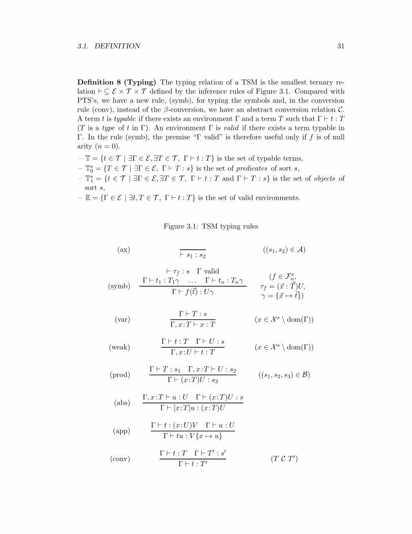
Definition 8 (Typing) The typing relation of a TSM is the smallest ternary re-lation ⊢⊆ E × T × T defined by the inference rules of Figure 3.1. Compared withPTS’s, we have a new rule, (symb), for typing the symbols and, in the conversionrule (conv), instead of the β-conversion, we have an abstract conversion relation C.A term t is typable if there exists an environment Γ and a term T such that Γ ⊢ t : T(T is a type of t in Γ). An environment Γ is valid if there exists a term typable inΓ. In the rule (symb), the premise “Γ valid” is therefore useful only if f is of nullarity (n = 0).
– T = {t ∈ T | ∃Γ ∈ E ,∃T ∈ T , Γ ⊢ t : T} is the set of typable terms,
– Ts0 = {T ∈ T | ∃Γ ∈ E , Γ ⊢ T : s} is the set of predicates of sort s,
– Ts1 = {t ∈ T | ∃Γ ∈ E ,∃T ∈ T , Γ ⊢ t : T and Γ ⊢ T : s} is the set of objects of
sort s,
– E = {Γ ∈ E | ∃t, T ∈ T , Γ ⊢ t : T} is the set of valid environments.
Figure 3.1: TSM typing rules
(ax)⊢ s1 : s2
((s1, s2) ∈ A)
(symb)
⊢ τf : s Γ validΓ ⊢ t1 : T1γ . . . Γ ⊢ tn : Tnγ
Γ ⊢ f(~t) : Uγ
(f ∈ Fsn,
τf = (~x : ~T )U,
γ = {~x 7→ ~t})
(var)Γ ⊢ T : s
Γ, x :T ⊢ x : T(x ∈ X s \ dom(Γ))
(weak)Γ ⊢ t : T Γ ⊢ U : s
Γ, x :U ⊢ t : T(x ∈ X s \ dom(Γ))
(prod)Γ ⊢ T : s1 Γ, x :T ⊢ U : s2
Γ ⊢ (x :T )U : s3((s1, s2, s3) ∈ B)
(abs)Γ, x :T ⊢ u : U Γ ⊢ (x :T )U : s
Γ ⊢ [x :T ]u : (x :T )U
(app)Γ ⊢ t : (x :U)V Γ ⊢ u : U
Γ ⊢ tu : V {x 7→ u}
(conv)Γ ⊢ t : T Γ ⊢ T ′ : s′
Γ ⊢ t : T ′(T C T ′)

32 CHAPTER 3. TYPE SYSTEMS MODULO
Remark 9 (Conversion)It might seem more natural to define (conv) in a symmetric way by adding the
premise Γ ⊢ T : s or the premise Γ ⊢ T : s′. We have chosen this definition for tworeasons. First, it is defined in this way in the reference papers on PTS’s [59, 10].Second, from a practical point of view, for type checking, this avoids an additionaltest. However, we will see in Lemma 37 that, for many TSM’s, we have Γ ⊢ T : s′.We will denote by ⊢s the typing relation defined by the same inference rules as for⊢ but with (conv) replaced by :
(conv’)Γ ⊢ t : T Γ ⊢ T : s Γ ⊢ T ′ : s
Γ ⊢ t : T ′(T C T ′)
We will show the equivalence between ⊢s and ⊢ in Lemma 43.In the same way, in full TSM’s (∀s1, s2 ∈ S,∃s3 ∈ S, (s1, s2, s3) ∈ B), the rule
(abs) can be replaced by :
(abs’)Γ, x :T ⊢ u : U
Γ ⊢ [x :T ]u : (x :T )U(U /∈ S or ∃s∈S, (U, s) ∈ A)
Finally, we will denote by ⊢w the typing relation defined by the same inferencerules as for ⊢ but with (weak) replaced by :
(weak’)Γ ⊢ t : T Γ ⊢ U : s
Γ, x :U ⊢ t : T(x ∈ X s \ dom(Γ), t ∈ X ∪ S)
that is, where weakening is restricted to variables and sorts (t ∈ X ∪ S). We willshow the equivalence between ⊢w and ⊢ in Lemma 19.
Remark 10 (Arity)On can wonder why symbols are equipped with a fixed arity since, in general,
in λ-calculus, one is used to consider higher-order constants. Of course, having anarity is not a restriction since, to a symbol f of arity n and type (~x : ~T )U , onecan always associate a curried version f c of null arity defined by the rewrite rulef c → [~x : ~T ]f(~x). Furthermore, in practice, the existence of arities can be masked bydoing η-expansions if f is not applied to sufficient arguments, or by doing additionalapplications if f is applied to too many arguments. However, without arities, wewould have a simpler presentation where the rule (symb) would be reduced to :
(symb’)⊢ τf : s
⊢ f : τf(f ∈ Fs)
To our knowledge, except the works of Jouannaud and Okada [75] and of G.Barthe and his co-authors [15, 16, 17, 13], most of the other works on the combinationof typed λ-calculi and rewriting [25, 26, 54] do not use arities for typing symbols.We have chosen to use arities for technical reasons. With the method we use forproving strong normalization, we need an application uv not to be a rewriting redex(see Chapter 5 for an explanation of these notions and Lemma 121, case T = (x :U)V , (b), (R3) for the use of this property). The introduction of arities enableus to syntactically distinguish between the application of the λ-calculus and theapplication of a symbol. But one may wonder whether this notion is really necessary.
3.2. PROPERTIES 33
Definition 11 (Well-typed substitution) Given two valid environments Γ and∆, a substitution θ is well typed between Γ and ∆ , θ : Γ→ ∆, if, for all x ∈ dom(Γ),∆ ⊢ xθ : xΓθ.
For example, in the rule (symb), we have γ : Γf → Γ where Γf = ~x : ~T .
3.2 Properties
In this section and the following one, we prove some properties of TSM’s that arewell known for PTS’s (except Lemma 22). Apart from the new case (symb) that wewill detail each time, proofs are identical to the ones for PTS’s. The fact that, in(conv), ↔∗
β is replaced by an arbitrary relation C is not important. For more details,the reader is invited to look at [59, 10, 58].
Lemma 12 (Free variables) Let Γ = ~x : ~T be an environment. If Γ ⊢ t : T then :
(a) the xi’s are distinct from one another,
(b) FV(t) ∪ FV(T ) ⊆ dom(Γ),
(c) for all i, FV(Ti) ⊆ {x1, . . . , xi−1}.
Proof. By induction on Γ ⊢ t : T . We only detail the new case (symb). (a) and(c) are true by induction hypothesis. Let us see (b) now. By induction hypothesis,FV(τf ) = ∅ and, for all i, FV(ti) ⊆ dom(Γ). Therefore, FV(f(~t)) ⊆ dom(Γ). Hence,FV(Uγ) ⊆ dom(Γ) since FV(U) ⊆ {~x} and γ = {~x 7→ ~t}. �
Lemma 13 (Subterms) If a term is typable then all its subterms are typable.
Proof. By induction on Γ ⊢ t : T . In the case of (symb), by induction hypoth-esis, for all i, all the subterms of ti are typable. Therefore, all the subterms of f(~t)are typable. �
Lemma 14 (Environment) Let Γ = ~x : ~T be a valid environment.
(a) If xi is of sort s then x1 :T1, . . . , xi−1 :Ti−1 ⊢ Ti : s.
(b) For all i, x1 :T1, . . . , xi :Ti ⊢ xi :Ti.
Proof. By (var), (b) is an immediate consequence of (a). We prove (a) byinduction on Γ ⊢ t : T . In the case (symb), as Γ is valid, there exists v and V suchthat Γ ⊢ v : V . Therefore, by induction hypothesis, (a) is true. �
The following lemma is a form of α-equivalence on the variables of an environ-ment.
Lemma 15 (Replacement) If Γ, y :W,Γ′ ⊢ t : T , y ∈ X s and z ∈ X s \ dom(Γ, y :W,Γ′) then Γ, z :W,Γ′{y 7→ z} ⊢ t{y 7→ z} : T{y 7→ z}.
Proof. By induction on Γ, y :W,Γ′ ⊢ t : T . Let θ = {y 7→ z}, ∆ = Γ, y :W,Γ′
and ∆′ = Γ, z :W,Γ′θ. In the case (symb), by induction hypothesis, we have ∆′ validand, for all i, ∆′ ⊢ tiθ : Tiγθ. Therefore, by (symb), ∆′ ⊢ f(~tθ) : Uγθ. �
34 CHAPTER 3. TYPE SYSTEMS MODULO
Lemma 16 (Weakening) If Γ ⊢ t : T and Γ ⊆ Γ′ ∈ E then Γ′ ⊢ t : T .
Proof. By induction on Γ ⊢ t : T . In the case (symb), by induction hypothesis,we have Γ′ valid and, for all i, Γ′ ⊢ ti : Tiγ. Therefore, by (symb), Γ′ ⊢ f(~t) : Uγ.�
Lemma 17 (Transitivity) Let Γ and ∆ be two valid environments. If Γ ⊢ t : Tand, for all x ∈ dom(Γ), ∆ ⊢ x : xΓ, that we will denote by ∆ ⊢ Γ, then ∆ ⊢ t : T .
Proof. By induction on Γ ⊢ t : T . In the case (symb), by induction hypothesis,we have ∆ valid and, for all i, ∆ ⊢ ti : Tiγ. Therefore, by (symb), ∆ ⊢ f(~t) : Uγ. �
Lemma 18 (Weak permutation) If Γ, y :A, z :B,Γ′ ⊢ t : T and Γ ⊢ B : s thenΓ, z :B, y :A,Γ′ ⊢ t : T .
Proof. Let ∆ = Γ, y : A, z : B,Γ′ and ∆′ = Γ, z : B, y : A,Γ′. By transitivity,it suffices to prove that ∆′ is valid and that ∆′ ⊢ ∆. And to this end, it sufficesto prove that ∆′ is valid. By the Environment Lemma, we have Γ ⊢ A : s′ and,by hypothesis, we have Γ ⊢ B : s. Therefore, by weakening, Γ, z : B, y : A isvalid. Assume that Γ′ = ~x : ~T and let ∆i = Γ, y : A, z : B,x1 : T1, . . . , xi : Ti and∆′
i = Γ, z :B, y :A, x1 :T1, . . . , xi :Ti. We prove by induction on i that ∆′i is valid. We
have already proved that ∆′0 is valid. Assume that ∆′
i is valid. By the EnvironmentLemma, ∆i ⊢ Ti+1 : si+1. As ∆
′i ⊢ ∆i, ∆
′i ⊢ Ti+1 : si+1 and ∆′
i+1 is valid. Therefore,∆′ is valid and ∆′ ⊢ t : T . �
Lemma 19 (Equivalence of ⊢w and ⊢) ⊢w =⊢.
Proof. First of all, it is clear that ⊢w ⊆⊢. We prove the reverse by induction onΓ ⊢ t : T . The only difficult case is of course (weak) : from Γ ⊢ t : T and Γ ⊢ U : s,we get Γ, x :U ⊢ t : T . By induction hypothesis, we have Γ ⊢w t : T and Γ ⊢w U : s.One has to modify the proof of Γ ⊢w t : T by adding x :U at the appropriate placesin order to obtain a proof of Γ, x :U ⊢w t : T . See Lemma 4.4.21 page 102 in [58] formore details. �
Now, let us see what we can do about the derivations of Γ ⊢ t : T and the formof T with respect to t. To this end, we introduce relations related to the rule (conv).
Definition 20 (Conversion relations)
– T CΓ T′ iff T C T ′ and there exists t, t′ and s′ such that Γ ⊢ t : T , Γ ⊢ t′ : T ′ and
Γ ⊢ T ′ : s′,
– T CΓ T′ iff T CΓ T
′ and there exists s such that Γ ⊢ T : s,
– Γ C Γ′ iff Γ = ~x : ~T , Γ′ = ~x : ~T ′ and, either |~x| = 0, or there exists j such thatTj Cx1:T1,...,xj−1:Tj−1
T ′j and, for all i 6= j, Ti = T ′
i .
We have CΓ ⊆ CΓ but, as opposed to CΓ, CΓ is not defined in a symmetric way.This comes from the asymmetry of the rule (conv) which requires Γ ⊢ T ′ : s′ butnot Γ ⊢ T : s. However, we will see in Lemma 37 that, for many TSM’s, these tworelations are equal.
Lemma 21 (Inversion) Assume that Γ ⊢ t : T .

3.3. TSM’S STABLE BY SUBSTITUTION 35
– If t = s then there exists s′ such that (s, s′) ∈ A and s′ C∗Γ T .
– If t = f(~t), f ∈ Fs, τf = (~x : ~T )U and γ = {~x 7→ ~t} then ⊢ τf : s, γ : (~x : ~T )→ Γand Uγ C∗Γ T .
– If t = x ∈ X s then Γ ⊢ xΓ : s and xΓ C∗Γ T .
– If t = (x :U)V then there exists (s1, s2, s3) ∈ P such that Γ ⊢ U : s1, Γ, x :U ⊢V : s2 and s3 C
∗Γ T .
– If t = [x :U ]v then there exists V such that Γ, x :U ⊢ v : V and (x :U)V C∗Γ T .
– If t = uv then there exists V and W such that Γ ⊢ u : (x :V )W , Γ ⊢ v : V andW{x 7→ v} C∗Γ T .
Proof. A typing derivation always finishes by a rule distinct from (weak) and(conv) followed by a possibly empty sequence of (weak)’s and (conv)’s. We henceget the term to which T is convertible. For typing judgments, it suffices to do aweakening to express them in Γ. �
Lemma 22 (Environment conversion) If Γ ⊢ t : T and Γ C Γ′ then Γ′ ⊢ t : T .
Proof. We have Γ = ~x : ~T , Γ′ = ~x : ~T ′ and there exists j such that Tj C∆ T ′j
with ∆ = x1 : T1, . . . , xj−1 : Tj−1 and, for all i 6= j, Ti = T ′i . By transitivity, it
suffices to prove that, for all i, Γ′ ⊢ xi : Ti. Let n = |~x|, Γ1 = x1 :T1, . . . , xj−1 :Tj−1
and Γ2 = xj+1 :Tj+1, . . . , xn :Tn. We proceed by induction on the size of Γ2.If Γ2 is empty then Γ = Γ1, xj : Tj and Γ′ = Γ1, xj : T
′j . Since Γ is valid, Γ1 is
valid and, for all i < j, Γ1 ⊢ xi : Ti. Since Tj CΓ1T ′j, there exists s and s′ such
that Γ1 ⊢ Tj : s and Γ1 ⊢ T′j : s
′. By (weak), we get, for all i < j, Γ′ ⊢ xi : Ti, andby (var), we get Γ′ ⊢ xj : T ′
j . From Γ1 ⊢ Tj : s, by (weak), we also get Γ′ ⊢ Tj : s.Therefore, by (conv), Γ′ ⊢ xj : Tj .
assume now that Γ2 = Γ3, xn :Tn. Let ∆ = Γ1, xj :Tj ,Γ3 and ∆′ = Γ1, xj :T′j ,Γ3.
By induction hypothesis, for all i < n, ∆′ ⊢ xi : Ti. Since Γ is valid, there exists ssuch that ∆ ⊢ Tn : s. By transitivity, we get ∆′ ⊢ Tn : s. Therefore, by (var), weget Γ′ ⊢ xn : Tn, and by (weak), Γ′ ⊢ xi : Ti. �
3.3 TSM’s stable by substitution
Definition 23 (TSM stable by substitution) A TSM is stable by substitutionif its conversion relation C is stable by substitution.
Lemma 24 (Substitution) If C is stable by substitution, Γ ⊢ t : T and θ : Γ→ ∆then ∆ ⊢ tθ : Tθ.
Proof. By induction on Γ ⊢ t : T . In the case (symb), by induction hypothesis,we have ∆ ⊢ tiθ : Tiγθ. Therefore, by (symb), ∆ ⊢ f(~tθ) : Uγθ. �
Corollary 25 If C is stable by substitution, Γ, x :U,Γ′ ⊢ t : T and Γ ⊢ u : U thenΓ,Γ′{x 7→ u} ⊢ t{x 7→ u} : T{x 7→ u}.
Proof. We have to prove that θ = {x 7→ u} is a well-typed substitution fromΓ, x :U,Γ′ to Γ,Γ′θ. We proceed by induction on the size of Γ′. If Γ′ is empty, this is

36 CHAPTER 3. TYPE SYSTEMS MODULO
immediate since Γ is valid and Γ ⊢ u : U . Assume now that Γ′ = Γ′′, y :V . Let ∆ =Γ, x :U,Γ′′ and ∆′ = Γ,Γ′′θ. By induction hypothesis, θ : ∆→ ∆′. Since ∆ ⊢ V : s,by substitution, we get ∆′ ⊢ V θ : s. Therefore, by (var), ∆′, y :V θ ⊢ y : V θ. Now,let z ∈ dom(∆). As ∆ ⊢ z : z∆, by substitution, ∆′ ⊢ z : z∆θ. Then, by (weak),∆′, y :V θ ⊢ z : z∆θ. �
Corollary 26 If C is stable by substitution, θ1 : Γ0 → Γ1 and θ2 : Γ1 → Γ2 thenθ1θ2 : Γ0 → Γ2.
Proof. Let x ∈ dom(Γ0). Since θ1 : Γ0 → Γ1, by substitution, we get Γ1 ⊢ xθ1 :xΓ0θ1, and since θ2 : Γ1 → Γ2, by substitution again, we get Γ2 ⊢ xθ1θ2 : xΓ0θ1θ2.�
Definition 27 (Maximal sort) A sort s is maximal if there does not exist anysort s′ such that (s, s′) ∈ A.
Lemma 28 (Correctness of types) If C is stable by substitution and Γ ⊢ t : Tthen, either T is a maximal sort, or there exists a sort s such that Γ ⊢ T : s. Inother words, T =
⋃
{Ts0 ∪ T
s1 | s ∈ S}.
Proof. By induction on Γ ⊢ t : T . In the case (symb), we have ⊢ τf : s. Byinversion, there exists s′ such that Γf ⊢ U : s′. As γ : Γf → Γ, by substitution,Γ ⊢ Uγ : s′. �
Lemma 29 (Inversion for TSM’s stable by substitution) Assume that Γ ⊢t : T .
– If t = s then there exists s′ such that (s, s′) ∈ A and s′ C∗Γ T .
– If t = f(~t), f ∈ Fs, τf = (~x : ~T )U and γ = {~x 7→ ~t} then ⊢ τf : s, γ : (~x : ~T )→ Γand Uγ C
∗Γ T .
– If t = x ∈ X s then Γ ⊢ xΓ : s and xΓ C∗Γ T .
– If t = (x :U)V then there exists (s1, s2, s3) ∈ P such that Γ ⊢ U : s1, Γ, x :U ⊢V : s2 and s3 C
∗Γ T .
– If t = [x :U ]v then there exists V such that Γ, x :U ⊢ v : V and (x :U)V C∗Γ T .
– If t = uv then there exists V and W such that Γ ⊢ u : (x :V )W , Γ ⊢ v : V andW{x 7→ v} C∗
Γ T .
Proof. Only the cases t = f(~t) and t = uv have been modified.
– t = f(~t). By inversion, ⊢ τf : s, γ : (~x : ~T )→ Γ and Uγ C∗Γ T . By inversion again,
there exists s′ such that ~x : ~T ⊢ U : s′. Therefore, by substitution, Γ ⊢ Uγ : s′
and Uγ C∗Γ T .
– t = uv. By inversion, there exists V and W such that Γ ⊢ u : (x : V )W ,Γ ⊢ v : V and W{x 7→ v} C∗Γ T . By correctness of types, there exists s suchthat Γ ⊢ (x : V )W : s. By inversion, there exists s′ such that Γ, x : V ⊢ W : s′.Therefore, by substitution, Γ ⊢W{x 7→ v} : s′ and W{x 7→ v} C∗
Γ T . �
3.4. LOGICAL TSM’S 37
3.4 Logical TSM’s
We now introduce an important class of TSM’s for which β-reduction preservestyping.
Definition 30 (Logical TSM) A TSM is logical if its conversion relation is prod-uct compatible :
(x :T )U C∗Γ (x′ :T ′)U ′ implies T C
∗Γ T
′ and U C∗Γ,x:T U ′{x′ 7→ x}.
T C∗Γ T
′ means that there exists a sequence of terms ~T such that T0 = T CΓ T1. . .Tn−1 CΓ Tn = T ′. So, there is no reason a priori to take U C
∗Γ,x:T U ′{x′ 7→ x}
instead of U C∗Γ,x:Ti
U ′{x′ 7→ x} with i 6= 0. However, as T C∗Γ T
′, by environmentconversion, this choice is not important.
Product compatibility is not a new condition and appears in all the previouslycited works but, to our knowledge, it has never received any special name.
All the TSM’s cited at the beginning of this chapter are logical. In the casewhere C =↔∗ with → a confluent reduction relation, it is clear that C is productcompatible. To prove this property without using confluence is more delicate. Thisis the case of PTS’s with η-reduction [58] or of the λR-cube [54], an extension of theCalculus of Constructions with higher-order rewriting a la Jouannaud-Okada at theobject-level.
Lemma 31 (Subject reduction for β) In a logical βTSM, if Γ ⊢ t : T and t→β
t′ then Γ ⊢ t′ : T .
Proof. We will say that an environment ~x : ~T β-rewrites to an environment~x′ : ~T ′, written ~x : ~T →β ~x
′ : ~T ′, if ~x = ~x′ and there exists j such that Tj →β T′j
and, for all i 6= j, Ti = T ′i . We simultaneously prove that :
(a) if t→β t′ then Γ ⊢ t′ : T ,
(b) if Γ→β Γ′ then Γ′ ⊢ t : T ,
by induction on Γ ⊢ t : T .
(ax) ⊢ s1 : s2 ((s1, s2) ∈ A)No β-reduction is possible in s1 or in Γ = ∅.
(symb)⊢ τf : s Γ valid Γ ⊢ t1 : T1γ . . .Γ ⊢ tn : Tnγ
Γ ⊢ f(~t) : Uγ
(f ∈ Fsn,
τf = (~x : ~T )U,
γ = {~x 7→ ~t})
(a) If f(~t)→β t′ then t′ = f(~t′) with j such that tj →β t
′j and, for all i 6= j, ti = t′i.
By induction hypothesis, we have, for all i, Γ ⊢ t′i : Tiγ. Let γ′ = {~x 7→ ~t′}.We have Uγ′∗← βUγ and, for all i, Tiγ →
∗β Tiγ
′. As ↓β⊆ C, Uγ′ C Uγ and
Tiγ C Tiγ′. If we prove that every Tiγ
′ is typable in Γ by a sort then, by(conv), we have Γ ⊢ t′i : Tiγ
′ and, by (symb), Γ ⊢ t′ : Uγ′. It then suffices toprove that Uγ is typable by a sort in Γ to apply again (conv) and concludethat Γ ⊢ t′ : Uγ.
38 CHAPTER 3. TYPE SYSTEMS MODULO
Let us begin by verifying that Uγ is typable by a sort. We have ⊢ τf : s.
By inversion, γ : (~x : ~T )→ Γ and there exists s′ such that ~x : ~T ⊢ U : s′. Bysubstitution, we therefore get Γ ⊢ Uγ : s′.
Now, we are going to prove that every Tiγ′ is typable by a sort. To this
end, it suffices to prove that γ′ : (~x : ~T ) → Γ. Indeed, since ⊢ τf : s, byinversion, every Ti is typable by a sort in Γi−1 = x1 :T1, . . . , xi−1 :Ti−1. Letus prove by induction on i that γ′ : Γi → Γ.
For i = 0, there is nothing to prove. Assume therefore that γ′ : Γi → Γ.Then γ′ : Γi+1 → Γ if Γ ⊢ t′i+1 : Ti+1γ
′. We know that Γ ⊢ t′i+1 : Ti+1γ,Ti+1γ →
∗β Ti+1γ
′ and that there exists s such that Γi ⊢ Ti+1 : s. Therefore,by substitution, Γ ⊢ Ti+1γ
′ : s and, by (conv), Γ ⊢ t′i+1 : Ti+1γ′.
(b) If Γ →β Γ′ then, by induction hypothesis, Γ′ is valid and Γ′ ⊢ ti : Tiγ.Therefore, by (symb), Γ′ ⊢ f(~t) : Uγ.
(var)Γ ⊢ T : s
Γ, x :T ⊢ x : T
(a) No β-reduction is possible in x.
(b) There is two cases, depending on where takes place the β-reduction :
– Γ →β Γ′. By induction hypothesis, Γ′ ⊢ T : s. Therefore, by (var), Γ′, x :T ⊢ x : T .
– T →β T ′. By induction hypothesis, Γ ⊢ T ′ : s. Therefore, by (var),Γ, x :T ′ ⊢ x : T ′. As ↓β⊆ C, T
′ C T . As Γ ⊢ T : s, by (conv), Γ, x :T ′ ⊢ x : T .
(weak)Γ ⊢ t : T Γ ⊢ U : s
Γ, x :U ⊢ t : T
(a) If t→β t′ then, by induction hypothesis, Γ ⊢ t′ : T . As Γ ⊢ U : s, by (weak),
Γ, x :U ⊢ t′ : T .
(b) There is two cases, depending on where takes place the β-reduction :
– Γ→β Γ′. By induction hypothesis, Γ′ ⊢ t : T and Γ′ ⊢ U : s. Therefore, by(weak), Γ′, x :U ⊢ t : T .
– U →β U ′. By induction hypothesis, Γ ⊢ U ′ : s. Therefore, by (weak),Γ, x :U ′ ⊢ t : T .
(prod)Γ ⊢ T : s1 Γ, x :T ⊢ U : s2
Γ ⊢ (x :T )U : s3((s1, s2, s3) ∈ B)
(a) There is two cases, depending on where takes place the β-reduction :
– T →β T ′. By induction hypothesis, Γ ⊢ T ′ : s1 and Γ, x : T ′ ⊢ U : s2.Therefore, by (prod), we get Γ ⊢ (x :T ′)U : s3.
– U →β U′. By induction hypothesis, Γ, x :T ⊢ U ′ : s2. Therefore, by (prod),
Γ ⊢ (x :T )U ′ : s3.
(b) If Γ →β Γ′ then, by induction hypothesis, Γ′ ⊢ T : s1 and Γ′, x :T ⊢ U : s2.Therefore, by (prod), Γ′ ⊢ (x :T )U : s3.
(abs)Γ, x :T ⊢ u : U Γ ⊢ (x :T )U : s
Γ ⊢ [x :T ]u : (x :T )U
(a) There is two cases, depending on where takes place the β-reduction :
3.4. LOGICAL TSM’S 39
– T →β T′. By induction hypothesis, Γ, x :T ′ ⊢ u : U and Γ ⊢ (x :T ′)U : s.
By (abs), Γ ⊢ [x : T ′]u : (x : T ′)U . As (x : T ′)U← β(x : T )U and ↓β⊆ C,(x :T ′)U C (x :T )U . As Γ ⊢ (x :T )U : s, by (conv), Γ ⊢ [x :T ′]u : (x :T )U .
– u →β u′. By induction hypothesis, Γ, x :T ⊢ u′ : U . As Γ ⊢ (x :T )U : s, by
(abs), Γ ⊢ [x :T ]u′ : (x :T )U .
(b) If Γ→β Γ′ then, by induction hypothesis, Γ′, x :T ⊢ u : U and Γ′ ⊢ (x :T )U : s.Therefore, by (abs), Γ′ ⊢ [x :T ]u : (x :T )U .
(app)Γ ⊢ t : (x :U)V Γ ⊢ u : U
Γ ⊢ tu : V {x 7→ u}
(a) There is three cases, depending on where takes place the β-reduction :
– t→β t′. By induction hypothesis, Γ ⊢ t′ : (x :U)V . As Γ ⊢ u : U , by (app),
Γ ⊢ t′u : V {x 7→ u}.
– u →β u′. By induction hypothesis, Γ ⊢ u′ : U . By (app), Γ ⊢ tu′ : V {x 7→
u′}. As V {x 7→ u′}∗← βV {x 7→ u} and ↓β⊆ C, V {x 7→ u′} C V {x 7→ u}. Byinversion, there exists s such that Γ ⊢ V {x 7→ u} : s. Therefore, by (conv),Γ ⊢ tu′ : V {x 7→ u}.
– t = [x :U ′]v and tu →β v{x 7→ u}. By inversion, there exists V ′ such thatΓ, x : U ′ ⊢ v : V ′ and (x : U ′)V ′
C∗Γ (x : U)V . By product compatibility,
U ′C∗Γ U and V ′
C∗Γ,x:U V . By environment conversion, Γ, x :U ⊢ v : V ′ and,
by (conv), Γ, x :U ⊢ v : V .
(b) If Γ →β Γ′ then, by induction hypothesis, Γ′ ⊢ t : (x : U)V Γ′ ⊢ u : U .Therefore, by (app), Γ′ ⊢ tu : V {x 7→ u}.
(conv)Γ ⊢ t : T T C T ′ Γ ⊢ T ′ : s′
Γ ⊢ t : T ′
(a) If t→β t′ then, by induction hypothesis, Γ ⊢ t′ : T . As T C T ′ and Γ ⊢ T ′ : s′,
by (conv), Γ ⊢ t′ : T ′.
(b) If Γ →β Γ′ then, by induction hypothesis, Γ′ ⊢ t : T and Γ′ ⊢ T ′ : s′.Therefore, by (conv), Γ′ ⊢ t : T ′. �

40 CHAPTER 3. TYPE SYSTEMS MODULO

Chapter 4
Reduction Type Systems(RTS’s)
Now, we are going to study the case of TSM’s whose conversion relation C is ofthe form ↓ with → a reduction relation. We shall call such systems ReductionType Systems (RTS). Except for ECC [81] which uses a notion of subtyping, allthe systems previously mentioned at the beginning of Chapter 3 are RTS’s, eitherbecause they are defined in this way [54, 15], or because they are defined with C =↔∗
and → confluent, which is equivalent [99, 58, 119, 101]. The general study of suchsystems is justified by the fact that, in [54], the proof that reduction preserves typinguses the fact that C is of the form ↓.
The proofs of the Lemmas 41, 47, 50 and 52 are widely inspired from the onesgiven by H. Geuvers and M.-J. Nederhof [59] or H. Geuvers [58].
4.1 Definition
Definition 32 (RTS) A pre-RTS is a TSM whose conversion relation C is of theform ↓ with → a relation stable by substitution and context. The relation → iscalled the reduction relation of the pre-RTS. A pre-RTS is confluent if its reductionrelation is confluent. An RTS is a pre-RTS which is admissible , that is, whosereduction relation preserves typing : Γ ⊢ t : T and t → t′ imply Γ ⊢ t′ : T , aproperty often called subject reduction .
Any pre-RTS satisfies the following elementary properties :
Lemma 33 The relation C =↓ is :
– symmetric : T C T ′ implies T ′ C T .
– stable by substitution : T C T ′ implies Tθ C T ′θ.
– stable by context : T C T ′ implies C[T ]p C C[T ′]p.
– preserves sorts : s C s′ implies s = s′.
In ECC, the conversion relation C is not symmetric and does not preserve sorts.It would be interesting to try to formulate some properties below in the more generalframework of Cumulative pure Type Systems (CTS) to which belongs ECC. To this
41
42 CHAPTER 4. REDUCTION TYPE SYSTEMS
end, the reader is refered to the works of Z. Luo [81], R. Pollack [102] and Barras[11].
Subject reduction can be extended to types, environments and substitutions :
Definition 34 A substitution θ rewrites to a substitution θ′, θ → θ′, if there existsx such that xθ → xθ′ and, for all y 6= x, yθ = yθ′. An environment Γ = ~x : ~Trewrites to an environment Γ′, Γ → Γ′, if Γ′ = ~x : ~T ′ and there exists i such thatTi → T ′
i and, for all j 6= i, Tj = T ′j .
Lemma 35 In an RTS :
(a) if Γ ⊢ t : T and T → T ′ then Γ ⊢ t : T ′,
(b) if θ : Γ→ ∆ and θ → θ′ then θ′ : Γ→ ∆,
(c) if Γ ⊢ t : T and Γ→ Γ′ then Γ′ ⊢ t : T .
Proof.
(a) By correctness of types, either T = s or Γ ⊢ T : s. The case T = s is notpossible since s is not reducible. Therefore, Γ ⊢ T : s and, by subject reduction,Γ ⊢ T ′ : s. Hence, by (conv), Γ ⊢ t : T ′.
(b) By induction on the size of Γ. If Γ is empty, this is immediate. Assume thenthat Γ = Γ′, x :T . Since θ : Γ′ → ∆, by induction hypothesis, θ′ : Γ′ → ∆. Thenit suffices to prove that ∆ ⊢ xθ′ : Tθ′. As θ : Γ→ ∆, we have ∆ ⊢ xθ : Tθ. Bysubject reduction, ∆ ⊢ xθ′ : Tθ. After the Environment Lemma, there exists ssuch that Γ ⊢ T : s. By substitution, ∆ ⊢ Tθ : s. Since Tθ →∗ Tθ′, Tθ C Tθ′
and, by subject reduction, ∆ ⊢ Tθ′ : s. Therefore, by (conv), ∆ ⊢ xθ′ : Tθ′.
(c) Assume that Γ = Γ1, x : T,Γ2 and Γ′ = Γ1, x : T ′,Γ2. By the EnvironmentLemma, Γ1 ⊢ T : s. By subject reduction, Γ1 ⊢ T
′ : s. Therefore, Γ C Γ′ and,by the Environment conversion Lemma, Γ′ ⊢ t : T . �
Lemma 36 (Inconvertibility of maximal sorts) In an RTS, if s C∗Γ T thens C
∗Γ T . Therefore, if s is maximal then T = s.
Proof. By case on the number of conversions between s and T . If s = T , thisis immediate. Assume then that s CΓ T
′ C∗Γ T . By definition of CΓ, there exists s′
such that Γ ⊢ T ′ : s′. As C =↓ and s is irreducible, T ′ →∗ s. By subject reduction,Γ ⊢ s : s′ and s C
∗Γ T . �
Hence we get the equivalence of the two relations CΓ and CΓ, and a refinementof the Inversion Lemma for RTS’s.
Lemma 37 (Equivalence of CΓ and CΓ) In an RTS, CΓ = CΓ.
Proof. First of all, we have CΓ ⊆ CΓ. We prove the reverse. Assume thatT CΓ T
′. As there exists t such that Γ ⊢ t : T , by correctness of types, either T isa maximal sort, or there exists s such that Γ ⊢ T : s. After the previous lemma, Tcannot be a maximal sort. Therefore, there exists s such that Γ ⊢ T : s and T CΓ T
′.�
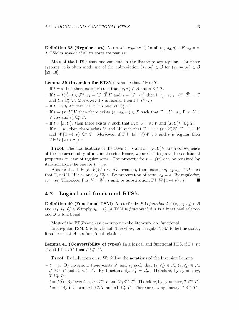
4.2. LOGICAL AND FUNCTIONAL RTS’S 43
Definition 38 (Regular sort) A sort s is regular if, for all (s1, s2, s) ∈ B, s2 = s.A TSM is regular if all its sorts are regular.
Most of the PTS’s that one can find in the literature are regular. For thesesystems, it is often made use of the abbreviation (s1, s2) ∈ B for (s1, s2, s2) ∈ B[59, 10].
Lemma 39 (Inversion for RTS’s) Assume that Γ ⊢ t : T .
– If t = s then there exists s′ such that (s, s′) ∈ A and s′ C∗Γ T .
– If t = f(~t), f ∈ Fs, τf = (~x : ~T )U and γ = {~x 7→ ~t} then ⊢ τf : s, γ : (~x : ~T )→ Γand Uγ C
∗Γ T . Moreover, if s is regular then Γ ⊢ Uγ : s.
– If t = x ∈ X s then Γ ⊢ xΓ : s and xΓ C∗Γ T .
– If t = (x :U)V then there exists (s1, s2, s3) ∈ P such that Γ ⊢ U : s1, Γ, x :U ⊢V : s2 and s3 C
∗Γ T .
– If t = [x :U ]v then there exists V such that Γ, x :U ⊢ v : V and (x :U)V C∗Γ T .
– If t = uv then there exists V and W such that Γ ⊢ u : (x : V )W , Γ ⊢ v : Vand W{x 7→ v} C
∗Γ T . Moreover, if Γ ⊢ (x : V )W : s and s is regular then
Γ ⊢W{x 7→ v} : s.
Proof. The modifications of the cases t = s and t = (x :U)V are a consequenceof the inconvertibility of maximal sorts. Hence, we are left to prove the additionalproperties in case of regular sorts. The property for t = f(~t) can be obtained byiteration from the one for t = uv.
Assume that Γ ⊢ (x : V )W : s. By inversion, there exists (s1, s2, s3) ∈ P suchthat Γ, x :V ⊢ W : s2 and s3 C
∗Γ s. By preservation of sorts, s3 = s. By regularity,
s2 = s3. Therefore, Γ, x :V ⊢W : s and, by substitution, Γ ⊢W{x 7→ v} : s. �
4.2 Logical and functional RTS’s
Definition 40 (Functional TSM) A set of rules B is functional if (s1, s2, s3) ∈ Band (s1, s2, s
′3) ∈ B imply s3 = s′3. A TSM is functional if A is a functional relation
and B is functional.
Most of the PTS’s one can encounter in the literature are functional.
In a regular TSM, B is functional. Therefore, for a regular TSM to be functional,it suffices that A is a functional relation.
Lemma 41 (Convertibility of types) In a logical and functional RTS, if Γ ⊢ t :T and Γ ⊢ t : T ′ then T C
∗Γ T
′.
Proof. By induction on t. We follow the notations of the Inversion Lemma.
– t = s. By inversion, there exists s′1 and s′2 such that (s, s′1) ∈ A, (s, s′2) ∈ A,
s′1 C∗Γ T and s′2 C
∗Γ T ′. By functionality, s′1 = s′2. Therefore, by symmetry,
T C∗Γ T
′.
– t = f(~t). By inversion, Uγ C∗Γ T and Uγ C
∗Γ T
′. Therefore, by symmetry, T C∗Γ T
′.
– t = x. By inversion, xΓ C∗Γ T and xΓ C
∗Γ T
′. Therefore, by symmetry, T C∗Γ T
′.

44 CHAPTER 4. REDUCTION TYPE SYSTEMS
– t = (x :U)V . By inversion, there exists (s1, s2, s3) ∈ P and (s′1, s′2, s
′3) ∈ P such
that Γ ⊢ U : s1, Γ ⊢ U : s′1, Γ, x : U ⊢ V : s2, Γ, x : U ⊢ V : s′2, s3 C∗Γ T and
s′3 C∗Γ T
′. By induction hypothesis, s1 C∗Γ s
′1 and s2 C
∗Γ,x:U s′2. By preservation of
sorts, s1 = s′1 and s2 = s′2. Therefore, by functionality, s3 = s′3 and, by symmetry,T C
∗Γ T
′.
– t = [x : U ]v. By inversion, there exists V and V ′ such that Γ, x : U ⊢ v : V ,Γ, x : U ⊢ v : V ′, (x : U)V C
∗Γ T and (x : U)V ′
C∗Γ T ′. By induction hypothesis,
V C∗Γ,x:U V ′. By stability by context, (x : U)V C
∗Γ (x : U)V ′. Therefore, by
symmetry, T C∗Γ T
′.
– t = uv. By inversion, there exists V , V ′, W and W ′ such that Γ ⊢ u : (x :V )W ,Γ ⊢ u : (x : V ′)W ′, W{x 7→ v} C
∗Γ T and W ′{x 7→ v} C
∗Γ T ′. By induction
hypothesis, (x :V )W C∗Γ (x :V ′)W ′. By product compatibility, W C
∗Γ,x:V W ′. By
substitution and stability by substitution, W{x 7→ v} C∗Γ W
′{x 7→ v}. Therefore,by symmetry, T C
∗Γ T
′. �
Lemma 42 (Conversion correctness) In a logical and functional RTS, if Γ ⊢ T :s and T CΓ T
′ then Γ ⊢ T ′ : s.
Proof. By definition of CΓ, there exists s′ such that Γ ⊢ T ′ : s′. As C = ↓, thereexists U such that T →∗ U and T ′ →∗ U . By subject reduction, Γ ⊢ U : s andΓ ⊢ U : s′. By convertibility of types and preservation of sorts, s = s′ and Γ ⊢ T ′ : s.
�
Lemma 43 (Equivalence of ⊢s and ⊢) In a logical and functional RTS, ⊢s =⊢.
Proof. First of all, it is immediate that ⊢s ⊆⊢. We show the inverse by inductionon Γ ⊢ t : T . The only difficult case is of course (conv). By induction hypothesis,we have Γ ⊢st : T and Γ ⊢sT
′ : s′. It is easy to verify that the Substitution Lemmaand the correctness of types are also valid for ⊢s. Hence, by correctness of types,either T is a maximal sort, or there exists s such that Γ ⊢sT : s. If T is a maximalsort s then T ′ →∗ s and s is typable, which is excluded. Therefore, Γ ⊢sT : s. Byconvertibility of types and preservation of sorts, s = s′ and, by (conv’), Γ ⊢st : T
′.�
Lemma 44 (α-equivalence) In a logical and functional RTS, if (x :T )U CΓ (x′ :T ′)U ′ then x and x′ are of the same sort and (x′ : T ′)U ′ is α-equivalent to (x :T ′)U ′{x′ 7→ x}.
Proof. Assume that x is of sort s and x′ is of sort s′. By definition of CΓ, wehave Γ ⊢ (x :T )U : s3 and Γ ⊢ (x′ :T ′)U ′ : s′3. By inversion, we have Γ, x :T ⊢ U : s1and Γ, x′ : T ′ ⊢ U ′ : s′1. By the Environment Lemma, we have Γ ⊢ T : s andΓ ⊢ T ′ : s′. By conversion correctness and preservation of sorts, s = s′. Therefore xand x′ are of the same sort and (x′ :T ′)U ′ is α-equivalent to (x :T ′)U ′{x′ 7→ x}. �
Lemma 45 (Maximal sort) In a logical and functional RTS, if s is a maximalsort and Γ ⊢ t : s then t is of the form (~x : ~t)s′. Moreover, if t C∗
Γ t′ then t′ is of the
form (~y : ~t′)s′ with |~y| = |~x|.
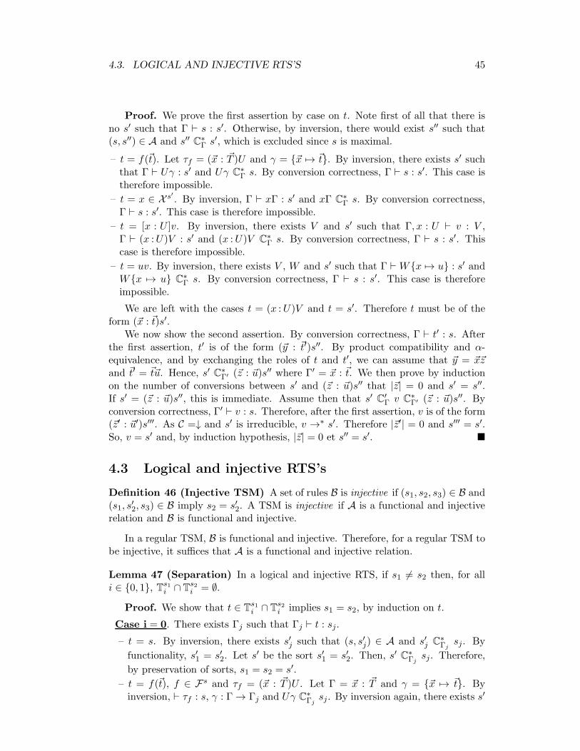
4.3. LOGICAL AND INJECTIVE RTS’S 45
Proof. We prove the first assertion by case on t. Note first of all that there isno s′ such that Γ ⊢ s : s′. Otherwise, by inversion, there would exist s′′ such that(s, s′′) ∈ A and s′′ C∗
Γ s′, which is excluded since s is maximal.
– t = f(~t). Let τf = (~x : ~T )U and γ = {~x 7→ ~t}. By inversion, there exists s′ suchthat Γ ⊢ Uγ : s′ and Uγ C
∗Γ s. By conversion correctness, Γ ⊢ s : s′. This case is
therefore impossible.
– t = x ∈ X s′ . By inversion, Γ ⊢ xΓ : s′ and xΓ C∗Γ s. By conversion correctness,
Γ ⊢ s : s′. This case is therefore impossible.
– t = [x : U ]v. By inversion, there exists V and s′ such that Γ, x : U ⊢ v : V ,Γ ⊢ (x :U)V : s′ and (x :U)V C
∗Γ s. By conversion correctness, Γ ⊢ s : s′. This
case is therefore impossible.
– t = uv. By inversion, there exists V , W and s′ such that Γ ⊢W{x 7→ u} : s′ andW{x 7→ u} C
∗Γ s. By conversion correctness, Γ ⊢ s : s′. This case is therefore
impossible.
We are left with the cases t = (x :U)V and t = s′. Therefore t must be of theform (~x : ~t)s′.
We now show the second assertion. By conversion correctness, Γ ⊢ t′ : s. Afterthe first assertion, t′ is of the form (~y : ~t′)s′′. By product compatibility and α-equivalence, and by exchanging the roles of t and t′, we can assume that ~y = ~x~zand ~t′ = ~t~u. Hence, s′ C∗
Γ′ (~z : ~u)s′′ where Γ′ = ~x : ~t. We then prove by inductionon the number of conversions between s′ and (~z : ~u)s′′ that |~z| = 0 and s′ = s′′.If s′ = (~z : ~u)s′′, this is immediate. Assume then that s′ C′
Γ v C∗Γ′ (~z : ~u)s′′. By
conversion correctness, Γ′ ⊢ v : s. Therefore, after the first assertion, v is of the form(~z′ : ~u′)s′′′. As C =↓ and s′ is irreducible, v →∗ s′. Therefore |~z′| = 0 and s′′′ = s′.So, v = s′ and, by induction hypothesis, |~z| = 0 et s′′ = s′. �
4.3 Logical and injective RTS’s
Definition 46 (Injective TSM) A set of rules B is injective if (s1, s2, s3) ∈ B and(s1, s
′2, s3) ∈ B imply s2 = s′2. A TSM is injective if A is a functional and injective
relation and B is functional and injective.
In a regular TSM, B is functional and injective. Therefore, for a regular TSM tobe injective, it suffices that A is a functional and injective relation.
Lemma 47 (Separation) In a logical and injective RTS, if s1 6= s2 then, for alli ∈ {0, 1}, Ts1
i ∩ Ts2i = ∅.
Proof. We show that t ∈ Ts1i ∩ T
s2i implies s1 = s2, by induction on t.
Case i = 0. There exists Γj such that Γj ⊢ t : sj.
– t = s. By inversion, there exists s′j such that (s, s′j) ∈ A and s′j C∗Γjsj. By
functionality, s′1 = s′2. Let s′ be the sort s′1 = s′2. Then, s′ C∗Γjsj. Therefore,
by preservation of sorts, s1 = s2 = s′.
– t = f(~t), f ∈ Fs and τf = (~x : ~T )U . Let Γ = ~x : ~T and γ = {~x 7→ ~t}. Byinversion, ⊢ τf : s, γ : Γ→ Γj and Uγ C
∗Γjsj. By inversion again, there exists s′
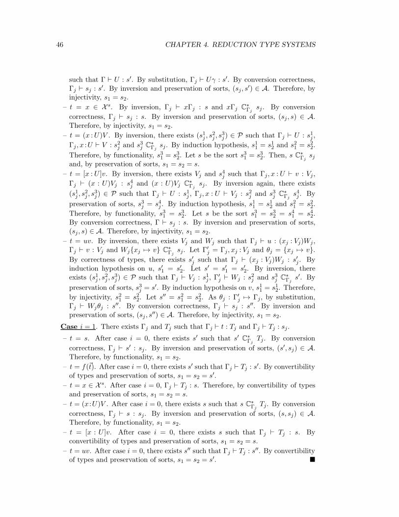
46 CHAPTER 4. REDUCTION TYPE SYSTEMS
such that Γ ⊢ U : s′. By substitution, Γj ⊢ Uγ : s′. By conversion correctness,Γj ⊢ sj : s
′. By inversion and preservation of sorts, (sj, s′) ∈ A. Therefore, by
injectivity, s1 = s2.
– t = x ∈ X s. By inversion, Γj ⊢ xΓj : s and xΓj C∗Γj
sj . By conversion
correctness, Γj ⊢ sj : s. By inversion and preservation of sorts, (sj, s) ∈ A.Therefore, by injectivity, s1 = s2.
– t = (x :U)V . By inversion, there exists (s1j , s2j , s
3j ) ∈ P such that Γj ⊢ U : s1j ,
Γj , x :U ⊢ V : s2j and s3j C∗Γjsj. By induction hypothesis, s11 = s12 and s21 = s22.
Therefore, by functionality, s31 = s32. Let s be the sort s31 = s32. Then, s C∗Γjsj
and, by preservation of sorts, s1 = s2 = s.
– t = [x : U ]v. By inversion, there exists Vj and s4j such that Γj, x : U ⊢ v : Vj ,
Γj ⊢ (x : U)Vj : s4j and (x : U)Vj C∗Γj
sj. By inversion again, there exists
(s1j , s2j , s
3j ) ∈ P such that Γj ⊢ U : s1j , Γj, x : U ⊢ Vj : s2j and s3j C
∗Γjs4j . By
preservation of sorts, s3j = s4j . By induction hypothesis, s11 = s12 and s21 = s22.
Therefore, by functionality, s31 = s32. Let s be the sort s31 = s32 = s41 = s42.By conversion correctness, Γ ⊢ sj : s. By inversion and preservation of sorts,(sj , s) ∈ A. Therefore, by injectivity, s1 = s2.
– t = uv. By inversion, there exists Vj and Wj such that Γj ⊢ u : (xj : Vj)Wj ,Γj ⊢ v : Vj and Wj{xj 7→ v} C
∗Γjsj. Let Γ′
j = Γj, xj : Vj and θj = {xj 7→ v}.
By correctness of types, there exists s′j such that Γj ⊢ (xj : Vj)Wj : s′j . Byinduction hypothesis on u, s′1 = s′2. Let s′ = s′1 = s′2. By inversion, thereexists (s1j , s
2j , s
3j) ∈ P such that Γj ⊢ Vj : s1j , Γ
′j ⊢ Wj : s2j and s3j C
∗Γjs′. By
preservation of sorts, s3j = s′. By induction hypothesis on v, s11 = s12. Therefore,
by injectivity, s21 = s22. Let s′′ = s21 = s22. As θj : Γ′j 7→ Γj, by substitution,
Γj ⊢ Wjθj : s′′. By conversion correctness, Γj ⊢ sj : s′′. By inversion andpreservation of sorts, (sj , s
′′) ∈ A. Therefore, by injectivity, s1 = s2.
Case i = 1. There exists Γj and Tj such that Γj ⊢ t : Tj and Γj ⊢ Tj : sj.
– t = s. After case i = 0, there exists s′ such that s′ C∗Γj
Tj . By conversion
correctness, Γj ⊢ s′ : sj. By inversion and preservation of sorts, (s′, sj) ∈ A.
Therefore, by functionality, s1 = s2.
– t = f(~t). After case i = 0, there exists s′ such that Γj ⊢ Tj : s′. By convertibility
of types and preservation of sorts, s1 = s2 = s′.
– t = x ∈ X s. After case i = 0, Γj ⊢ Tj : s. Therefore, by convertibility of typesand preservation of sorts, s1 = s2 = s.
– t = (x :U)V . After case i = 0, there exists s such that s C∗ΓjTj. By conversion
correctness, Γj ⊢ s : sj. By inversion and preservation of sorts, (s, sj) ∈ A.Therefore, by functionality, s1 = s2.
– t = [x : U ]v. After case i = 0, there exists s such that Γj ⊢ Tj : s. Byconvertibility of types and preservation of sorts, s1 = s2 = s.
– t = uv. After case i = 0, there exists s′′ such that Γj ⊢ Tj : s′′. By convertibility
of types and preservation of sorts, s1 = s2 = s′. �

4.3. LOGICAL AND INJECTIVE RTS’S 47
Lemma 48 (Classification) In a logical and injective RTS, either (s1, s2) ∈ Aand T
s10 ⊆ T
s21 , or (s1, s2) /∈ A and T
s10 ∩ T
s21 = ∅.
Proof. If (s1, s2) ∈ A, it is clear that Ts10 ⊆ T
s21 . We then prove that t ∈ T
s10 ∩T
s21
implies (s1, s2) ∈ A, by induction on t. Let Γ, Γ′ and T such that Γ ⊢ t : s1, Γ′ ⊢ t : T
and Γ′ ⊢ T : s2.
– t = s. By inversion, there exists s′1 and s′2 such that (s, s′1) ∈ A, s′1 C
∗Γ s1,
(s, s′2) ∈ A and s′2 C∗Γ′ T . By preservation of sorts, s′1 = s1. By functionality,
s′1 = s′2. By conversion correctness, Γ ⊢ s′2 : s2. Therefore, by inversion andpreservation of sorts, (s′2, s2) ∈ A and (s1, s2) ∈ A.
– t = f(~t). Let τf = (~x : ~T )U and γ = {~x 7→ ~t}. By inversion, there exists s′1and s′2 such that Γ ⊢ Uγ : s′1, Uγ C
∗Γ s1, Γ′ ⊢ Uγ : s′2 and Uγ C
∗Γ′ T . By
conversion correctness, Γ ⊢ s1 : s′1. Therefore, by inversion and preservation ofsorts, (s1, s
′1) ∈ A. By separation, s′1 = s′2. By conversion correctness, Γ′ ⊢ T : s′2.
Therefore, by separation, s′2 = s2 and (s1, s2) ∈ A.
– t = x ∈ X s. By inversion, Γ ⊢ xΓ : s, xΓ C∗Γ s1, Γ
′ ⊢ xΓ′ : s and xΓ′C∗Γ′ T .
By conversion correctness, Γ ⊢ s1 : s. By inversion and preservation of sorts,(s1, s) ∈ A. By conversion correctness, Γ′ ⊢ T : s. Therefore, by separation,s = s2 and (s1, s2) ∈ A.
– t = (x :U)V . By inversion, there exists (sa, sb, sc) and (s′a, s′b, s
′c) ∈ P such that
Γ ⊢ U : sa, Γ, x :U ⊢ V : sb, sc C∗Γ s1, Γ
′ ⊢ U : s′a, Γ′, x :U ⊢ V : s′b and s
′c C
∗Γ′ T .
By preservation of sorts, sc = s1. By conversion correctness, Γ′ ⊢ s′c : s2. Byinversion and preservation of sorts, (s′c, s2) ∈ A. By separation, sa = s′a andsb = s′b. Therefore, by functionality, sc = s′c and (s1, s2) ∈ A.
– t = [x :U ]v. By inversion, there exists V , s, V ′ and s′ such that Γ, x :U ⊢ v : V ,Γ ⊢ (x : U)V : s, (x : U)V C
∗Γ s1, Γ
′, x : U ⊢ v : V ′, Γ′ ⊢ (x : U)V ′ : s′ and(x : U)V ′
C∗Γ′ T . By conversion correctness, Γ ⊢ s1 : s and Γ′ ⊢ T : s′. By
inversion and preservation of sorts, (s1, s) ∈ A. By separation s′ = s2. Byinversion again, there exists (sa, sb, sc) and (s′a, s
′b, s
′c) ∈ P such that Γ ⊢ U : sa,
Γ, x : U ⊢ V : sb, sc C∗Γ s, Γ′ ⊢ U : s′a and Γ′, x : U ⊢ V ′ : s′b and s′c C
∗Γ′ s′. By
preservation of sorts, sc = s and s′c = s′. By separation, sa = s′a and sb = s′b.Therefore, by functionality, sc = s′c and (s1, s2) ∈ A.
– t = uv. By inversion, there exists V , W , s, V ′ and W ′ and s′ such that Γ ⊢u : (x : V )W , Γ ⊢ W{x 7→ v} : s, W{x 7→ v} C
∗Γ s1, Γ′ ⊢ u : (x : V ′)W ′,
Γ′ ⊢W ′{x 7→ v} : s′ and W ′{x 7→ v} C∗Γ′ T . By conversion correctness, Γ ⊢ s1 : s
and Γ′ ⊢ T : s′. By inversion and preservation of sorts, (s1, s) ∈ A. By separation,s = s′ and s′ = s2. Therefore, (s1, s2) ∈ A. �
Remark 49 (Typing classes)With the correctness of types, we have seen that a typable term is necessarily in
one of the sets Tsi where i ∈ {0, 1} and s ∈ S. With the Separation and Classification
Lemmas, we can describe the relations between these sets more precisely.In an injective TSM, the set of axioms A is necessarily an union of disjoint
maximal “chains”, that is, sets A′ such that :
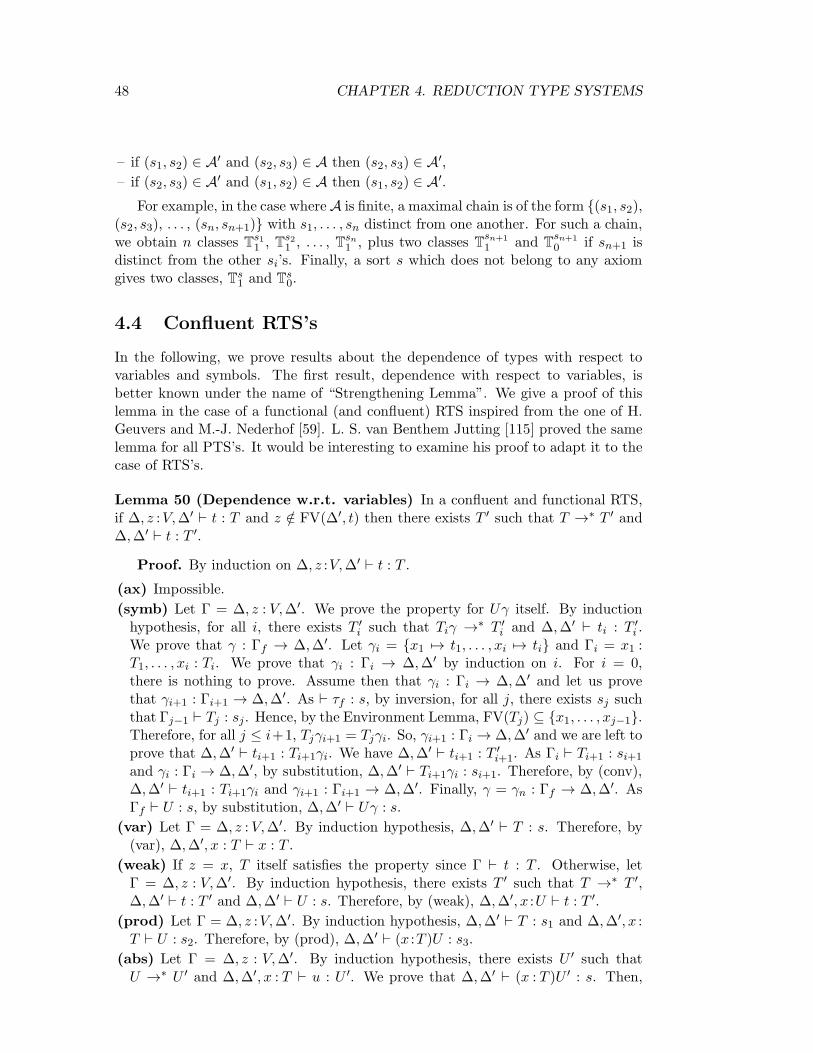
48 CHAPTER 4. REDUCTION TYPE SYSTEMS
– if (s1, s2) ∈ A′ and (s2, s3) ∈ A then (s2, s3) ∈ A
′,
– if (s2, s3) ∈ A′ and (s1, s2) ∈ A then (s1, s2) ∈ A
′.
For example, in the case whereA is finite, a maximal chain is of the form {(s1, s2),(s2, s3), . . . , (sn, sn+1)} with s1, . . . , sn distinct from one another. For such a chain,we obtain n classes T
s11 , Ts2
1 , . . . , Tsn1 , plus two classes T
sn+1
1 and Tsn+1
0 if sn+1 isdistinct from the other si’s. Finally, a sort s which does not belong to any axiomgives two classes, Ts
1 and Ts0.
4.4 Confluent RTS’s
In the following, we prove results about the dependence of types with respect tovariables and symbols. The first result, dependence with respect to variables, isbetter known under the name of “Strengthening Lemma”. We give a proof of thislemma in the case of a functional (and confluent) RTS inspired from the one of H.Geuvers and M.-J. Nederhof [59]. L. S. van Benthem Jutting [115] proved the samelemma for all PTS’s. It would be interesting to examine his proof to adapt it to thecase of RTS’s.
Lemma 50 (Dependence w.r.t. variables) In a confluent and functional RTS,if ∆, z :V,∆′ ⊢ t : T and z /∈ FV(∆′, t) then there exists T ′ such that T →∗ T ′ and∆,∆′ ⊢ t : T ′.
Proof. By induction on ∆, z :V,∆′ ⊢ t : T .
(ax) Impossible.
(symb) Let Γ = ∆, z : V,∆′. We prove the property for Uγ itself. By inductionhypothesis, for all i, there exists T ′
i such that Tiγ →∗ T ′
i and ∆,∆′ ⊢ ti : T ′i .
We prove that γ : Γf → ∆,∆′. Let γi = {x1 7→ t1, . . . , xi 7→ ti} and Γi = x1 :T1, . . . , xi : Ti. We prove that γi : Γi → ∆,∆′ by induction on i. For i = 0,there is nothing to prove. Assume then that γi : Γi → ∆,∆′ and let us provethat γi+1 : Γi+1 → ∆,∆′. As ⊢ τf : s, by inversion, for all j, there exists sj suchthat Γj−1 ⊢ Tj : sj. Hence, by the Environment Lemma, FV(Tj) ⊆ {x1, . . . , xj−1}.Therefore, for all j ≤ i+1, Tjγi+1 = Tjγi. So, γi+1 : Γi → ∆,∆′ and we are left toprove that ∆,∆′ ⊢ ti+1 : Ti+1γi. We have ∆,∆′ ⊢ ti+1 : T ′
i+1. As Γi ⊢ Ti+1 : si+1
and γi : Γi → ∆,∆′, by substitution, ∆,∆′ ⊢ Ti+1γi : si+1. Therefore, by (conv),∆,∆′ ⊢ ti+1 : Ti+1γi and γi+1 : Γi+1 → ∆,∆′. Finally, γ = γn : Γf → ∆,∆′. AsΓf ⊢ U : s, by substitution, ∆,∆′ ⊢ Uγ : s.
(var) Let Γ = ∆, z : V,∆′. By induction hypothesis, ∆,∆′ ⊢ T : s. Therefore, by(var), ∆,∆′, x : T ⊢ x : T .
(weak) If z = x, T itself satisfies the property since Γ ⊢ t : T . Otherwise, letΓ = ∆, z : V,∆′. By induction hypothesis, there exists T ′ such that T →∗ T ′,∆,∆′ ⊢ t : T ′ and ∆,∆′ ⊢ U : s. Therefore, by (weak), ∆,∆′, x :U ⊢ t : T ′.
(prod) Let Γ = ∆, z :V,∆′. By induction hypothesis, ∆,∆′ ⊢ T : s1 and ∆,∆′, x :T ⊢ U : s2. Therefore, by (prod), ∆,∆′ ⊢ (x :T )U : s3.
(abs) Let Γ = ∆, z : V,∆′. By induction hypothesis, there exists U ′ such thatU →∗ U ′ and ∆,∆′, x : T ⊢ u : U ′. We prove that ∆,∆′ ⊢ (x : T )U ′ : s. Then,
4.4. CONFLUENT RTS’S 49
by (abs), ∆,∆′ ⊢ [x : T ]u : (x : T )U ′. As Γ ⊢ (x : T )U : s, by inversion, thereexists (s1, s2, s) ∈ P such that Γ ⊢ T : s1 and Γ, x : T ⊢ U : s2. As z /∈ FV(T ),by induction hypothesis, ∆,∆′ ⊢ T : s1. As ∆,∆′, x :T ⊢ u : U ′, by correctnessof types, either U ′ = s′ or ∆,∆′, x : T ⊢ U ′ : s′. Assume that U ′ = s′. AsΓ, x : T ⊢ U : s2, by subject reduction, Γ, x : T ⊢ U ′ : s2. Therefore (s′, s2) ∈ Aand ∆,∆′, x : T ⊢ U ′ : s2. If now ∆,∆′, x : T ⊢ U ′ : s′ then, by convertibilityof types, s′ = s2. Hence, in all cases, Γ, x : T ⊢ U ′ : s2. Therefore, by (prod),∆,∆′ ⊢ (x :T )U ′ : s.
(app) Let Γ = ∆, z : V,∆′. By induction hypothesis, there exists U ′1, U
′2 and V
such that U →∗ U ′1, U →
∗ U ′2, V →
∗ V ′, ∆,∆′ ⊢ t : (x :U ′1)V
′ and ∆,∆′ ⊢ u : U ′2.
By confluence, there exists U ′′ such that U ′1 →
∗ U ′′ and U ′2 →
∗ U ′′. By subjectreduction, ∆,∆′ ⊢ t : (x : U ′′)V ′ and ∆,∆′ ⊢ u : U ′′. Therefore, by (app),∆,∆′ ⊢ tu : V ′{x 7→ u}.
(conv) By induction hypothesis, there exists T ′′ such that T →∗ T ′′ and ∆,∆′ ⊢t : T ′′. By confluence, there exists T ′′′ such that T ′′ →∗ T ′′′ and T ′ →∗ T ′′′. Bysubject reduction, ∆,∆′ ⊢ t : T ′′′. �
Corollary 51 In a confluent and functional RTS, if ∆, z : V,∆′ ⊢ t : T and z /∈FV(∆′, t, T ) then ∆,∆′ ⊢ t : T .
Proof. After the lemma, there exists T ′ such that T →∗ T ′ and ∆,∆′ ⊢ t : T ′.By correctness of types, either T is a maximal sort and T ′ = T , or ∆, z :V,∆′ ⊢ T : s.Then, after the lemma, ∆,∆′ ⊢ T : s. Therefore, by (conv), ∆,∆′ ⊢ t : T . �
Lemma 52 (Strong permutation) If Γ, y : A, z : B,Γ′ ⊢ t : T and y /∈ FV(B)then Γ, z :B, y :A,Γ′ ⊢ t : T .
Proof. Let ∆ = Γ, y :A, z :B,Γ′ and ∆′ = Γ, z :B, y :A,Γ′. By transitivity, itsuffices to prove that ∆′ is valid and that ∆′ ⊢ ∆. To this end, it suffices to provethat ∆′ is valid. By the Environment Lemma, we have Γ ⊢ A : s and Γ, y :A ⊢ B : s′.After the previous lemma, Γ ⊢ B : s′. Therefore, Γ, z :B is valid and, by weakening,Γ, z :B, y :A too. Assume that Γ′ = ~x : ~T and let ∆i = Γ, y :A, z :B,x1 :T1, . . . , xi :Tiand ∆′
i = Γ, z : B, y : A, x1 : T1, . . . , xi : Ti. We prove by induction on i that ∆′i is
valid. We have already proved that ∆′0 is valid. Assume that ∆′
i is valid. By theEnvironment Lemma, ∆i ⊢ Ti+1 : si+1. As ∆′
i ⊢ ∆i, ∆′i ⊢ Ti+1 : si+1 and ∆′
i+1 isvalid. Therefore, ∆′ is valid and ∆′ ⊢ t : T . �
Definition 53 (Compatibility w.r.t. a quasi-ordering) Let ≥ be a quasi-ordering on F . Given a symbol g, we will denote by ⊢g the typing relation of theRTS whose symbols are strictly smaller than g.
– → is compatible with ≥ if, for all symbol g and all term t, t′, if all the symbols int are strictly smaller than g and t→ t′ then the symbols in t′ are strictly smallerthan g.
– τ is compatible with ≥ if, for all symbol g, all the symbols in τg are smaller thang.
50 CHAPTER 4. REDUCTION TYPE SYSTEMS
Lemma 54 (Dependence w.r.t. symbols) Consider a confluent and functionalRTS and ≥ a quasi-ordering on F such that → and τ are compatible with ≥. IfΓ ⊢ t : T and the symbols in Γ and t are strictly smaller than g then there exists T ′
such that T →∗ T ′ and Γ ⊢g t : T′.
Proof. By induction on Γ ⊢ t : T .
(ax) Immediate.
(symb) We prove that Γ ⊢g f(~t) : Uγ. By induction hypothesis, for all i, thereexists T ′
i such that Tiγ →∗ T ′
i and Γ ⊢g ti : T′i . We prove that γ : Γf → Γ in
⊢g. Let γi = {x1 7→ t1, . . . , xi 7→ ti} and Γi = x1 : T1, . . . , xi : Ti. We prove thatγi : Γi → Γ by induction on i. For i = 0, there is nothing to prove. Assume thenthat γi : Γi → Γ and let us prove that γi+1 : Γi+1 → Γ. As τ is compatible with ≥,by induction hypothesis, ⊢g τf : s. By inversion, for all j, there exists sj such thatΓj−1 ⊢g Tj : sj. Hence, by the Free variables Lemma, FV(Tj) ⊆ {x1, . . . , xj−1}.Therefore, for all j ≤ i + 1, Tjγi+1 = Tjγi. So, γi+1 : Γi → Γ and we are left toprove that Γ ⊢g ti+1 : Ti+1γi. We have Γ ⊢g ti+1 : T ′
i+1. As Γi ⊢g Ti+1 : si+1
and γi : Γi → Γ, by substitution, Γ ⊢g Ti+1γi : si+1. Therefore, by (conv),Γ ⊢g ti+1 : Ti+1γi and γi+1 : Γi+1 → Γ. Finally, γ = γn : Γf → Γ. As Γf ⊢g U : s,by substitution, Γ ⊢g Uγ : s.
(var) By induction hypothesis, Γ ⊢g T : s. Therefore, by (var), Γ, x :T ⊢g x : T .
(weak) By induction hypothesis, there exists T ′ such that T →∗ T ′, Γ ⊢g t : T′
and Γ ⊢g U : s. Therefore, by (weak), Γ, x :U ⊢g t : T′.
(prod) By induction hypothesis, Γ ⊢g T : s1 and Γ, x :T ⊢g U : s2. Therefore, by(prod), Γ ⊢g (x :T )U : s3.
(abs) By induction hypothesis, there exists U ′ such that U →∗ U ′ and Γ, x :T ⊢g u :U ′. We prove that Γ ⊢g (x :T )U ′ : s. Then, by (abs), Γ ⊢g [x :T ]u : (x :T )U ′. AsΓ ⊢ (x :T )U : s, by inversion, there exists (s1, s2, s) ∈ P such that Γ ⊢ T : s1 andΓ, x :T ⊢ U : s2. By induction hypothesis, Γ ⊢g T : s1. As Γ, x :T ⊢g u : U ′, bycorrectness of types, either U ′ = s′ or Γ, x :T ⊢g U
′ : s′. Assume that U ′ = s′. AsΓ, x :T ⊢ U : s2, by subject reduction, Γ, x :T ⊢ U ′ : s2. Therefore (s
′, s2) ∈ A andΓ, x :T ⊢g U
′ : s2. If now Γ, x :T ⊢g U′ : s′ then, by convertibility of types, s′ = s2.
Hence, in all cases, Γ, x :T ⊢g U′ : s2. Therefore, by (prod), Γ ⊢g (x :T )U
′ : s.
(app) By induction hypothesis, there exists U ′1, U
′2 and V such that U →∗ U ′
1,U →∗ U ′
2, V →∗ V ′, Γ ⊢g t : (x :U
′1)V
′ and Γ ⊢g u : U ′2. By confluence, there exists
U ′′ such that U ′1 →
∗ U ′′ and U ′2 →
∗ U ′′. By subject reduction, Γ ⊢g t : (x :U′′)V ′
and Γ ⊢g u : U ′′. Therefore, by (app), Γ ⊢g tu : V ′{x 7→ u}.
(conv) By induction hypothesis, there exists T ′′ such that T →∗ T ′′ and Γ ⊢g t : T′′.
By confluence, there exists T ′′′ such that T ′′ →∗ T ′′′ and T ′ →∗ T ′′′. By subjectreduction, Γ ⊢g t : T
′′′. As→ is compatible with ≥, the symbols in T ′′′ are strictlysmaller than g. �

Chapter 5
Algebraic Type Systems (ATS’s)
Now, we are going to study the case of RTS’s whose reduction relation is made ofβ-reduction and rewrite rules. But, before, we must properly define what rewritingmeans in a strongly typed higher-order framework.
In first-order frameworks, that is, within a first-order term algebra, a rewriterule is generally defined as a pair l→ r of terms such that l is not a variable and thevariables occurring in r also occur in l (otherwise, rewriting does not terminate).Then, one says that a term t rewrites to a term t′ at position p if there exists asubstitution σ such that t|p = lσ (one says that t|p matches l) and t′ = t[rσ]p (thesubterm of t at position p, lσ, is replaced by rσ). The reader is invited to look at,for example, [46, 3] to get more details on first-order rewriting.
Here, we are going to consider a very similar rewriting mechanism by restrictingleft-hand sides of rules to belong to the first-order-like term algebra generated fromF and X . On the other hand, right-hand sides can be arbitrary. This is a particularthe case of Combinatory Reduction System (CRS) 1 of W. Klop [79] for which it isnot necessary to use higher-order pattern matching a la Klop or a la Miller [91, 95].
However, we proved in [21] that a weaker version of the termination criteria thatwe are going to present in next chapter can be adapted, in case of simply-typedλ-calculus, to rewriting with higher-order matching a la Klop or a la Miller. Itwould therefore be interesting to try to define a notion of rewriting with higher-order matching in case of polymorphic and dependent types, and to study if ourtermination criteria can also be adapted to this notion of rewriting.
Definition 55 (Algebraic terms) A term is algebraic if it is a variable or of theform f(~t) with all the ti’s themselves algebraic. We denote by T (F ,X ) the set ofalgebraic terms built from F and X , and by T(F ,X ) the set of typable algebraicterms.
Definition 56 (Rewriting) A rewrite rule is a pair of terms l → r such that lis an algebraic term distinct from a variable and FV(r) ⊆ FV(l). A rule l → r isleft-linear if no variable occurs more than once in l.
1To see this, it suffices to translate [x : T ]u by Λ(T, [x]u), (x : T )U by Π(T, [x]U) and uv by@(u, v), where Λ, Π and @ are symbols of arity 2 and [ ] is the abstraction operator of CRS’s.
51
52 CHAPTER 5. ALGEBRAIC TYPE SYSTEMS
Given a set of rewrite rulesR,R-reduction →R is the smallest relation containingR and stable by substitution and context. A term of the form lσ with l → r ∈ Rand σ a substitution is an R-redex .
Given a set of symbols G, we denote by RG the set of rules which define a symbolin G, that is, the set of rules such that the head symbol of the left-hand side is asymbol of G.
A symbol f is constant if R{f} = ∅, otherwise it is (partially) defined . Wedenote by CF the set of constant symbols and by DF the set of defined symbols.
Definition 57 (ATS) An ATS is a pre-RTS whose reduction relation → is of theform →R ∪ →β with R a set of rewrite rules.
Now that we have introduced our notion of rewriting, we can wonder under whichconditions it has the subject reduction property.
With first-order rewriting in sorted algebras, for rewriting to preserve the sortof terms, it suffices that, for all rules, both sides of the rule have the same sort.
Carried over to type systems, this condition gives : there exists an environmentΓ and a type T such that Γ ⊢ l : T and Γ ⊢ r : T . This condition is the one whichhas been taken in all previous work combining typed λ-calculus and rewriting.
However, this condition has an important drawback. With polymorphic or de-pendent types, it leads to strongly non-left-linear rules. This has two importantconsequences. First, rewriting is strongly slowed down because of the necessaryequality tests. Second, it is more difficult to prove confluence with non-left-linearrules.
Let us take the example of the concatenation of two polymorphic lists in the Cal-culus of Constructions (S = {⋆,✷}, A = {(⋆,✷)} and B = {(s1, s2, s3) ∈ S
3 | s2 =s3}) :
– list ∈ F✷
1 with τlist = ⋆→ ⋆ the type of polymorphic lists,
– nil ∈ F⋆1 with τnil = (A :⋆)list(A) the empty list,
– cons ∈ F⋆3 with τcons = (A : ⋆)A → list(A) → list(A) the function adding an
element at the head of a list,
– app ∈ F⋆3 with τapp = (A : ⋆)list(A) → list(A) → list(A) the concatenation
function.
A usual definition for app is :
– app(A,nil(A), ℓ′)→ ℓ′
– app(A, cons(A, x, ℓ), ℓ′)→ cons(A, x, app(A, ℓ, ℓ′))
This definition satisfies the usual condition; it suffices to take Γ = A :⋆, x :A, ℓ :list(A), ℓ′ : list(A) and T = list(A). But one may wonder whether it is really neces-sary to do an equality test between the first argument of app and the first argumentof cons when one wants to apply the second rule. Indeed, if app(A, cons(A′, x, ℓ), ℓ′)is well typed then, by inversion, cons(A′, x, ℓ) is of type list(A) and, by inversionagain, list(A′) is convertible to list(A). Hence, to allow the reduction even thoughA′ is different from A does not seem to be harmful since list(A′) is convertible tolist(A).

53
In fact, what is important is not that the left-hand side of a rule is typable, butthat, if an instance of the left-hand side of a rule is typable, then the correspondinginstance of the right-hand side has the same type. We express this by requiringthat there exists an environment Γ in which the right-hand side is typable, and asubstitution ρ which replaces the variables of the left-hand side not belonging to Γby terms typable typable in Γ. Hence, one can consider the following rules :
– app(A,nil(A′), ℓ′)→ ℓ′
– app(A, cons(A′, x, ℓ), ℓ′)→ cons(A, x, app(A, ℓ, ℓ′))
by taking Γ = A : ⋆, x : A, ℓ : list(A), ℓ′ : list(A) and ρ = {A′ 7→ A}. In [20],we give 5 conditions, (S1) to (S5), which must be satisfied by the rule l → r, Γand ρ. Assume that l = f(~l), τf = (~x : ~T )U and γ = {~x 7→ ~l}. Then, (S1)is dom(ρ) ⊆ FV(l) \ dom(Γ) and (S2) is Γ ⊢ lρ : Uγρ. Although these two firstconditions are often true, they are not necessary for proving the subject reductionproperty. This is why, in the following definition, they are not written. However,we will see that (S2) is necessary for proving the strong normalization property (seeDefinition 81).
Definition 58 (Well-typed rule) A rule l → r is well-typed if there exists anenvironment Γ and a substitution ρ such that, if l = f(~l), τf = (~x : ~T )U and
γ = {~x 7→ ~l} then :
(S3) Γ ⊢ r : Uγρ,
(S4) for all ∆, σ and T , if ∆ ⊢ lσ : T then σ : Γ→ ∆,
(S5) for all ∆, σ and T , if ∆ ⊢ lσ : T then, for all x, xσ ↓ xρσ.
In the following, we will write (l → r,Γ, ρ) ∈ R when the previous conditions aresatisfied.
An example using a dependent type is given by the concatenation of two listsof given length and the function map which, to a function f and a list a1 . . . an,associates the list f(a1) . . . f(an) :
– T ∈ F✷
0 with τT = ⋆ a type constant,
– nat ∈ F✷
0 with τnat = ⋆ the type of natural numbers,
– 0 ∈ F⋆0 with τ0 = nat zero,
– s ∈ F⋆1 with τs = nat→ nat the successor function,
– + ∈ F⋆2 with τ+ = nat→ nat→ nat the addition on nat,
– listn ∈ F✷
1 with τlistn = nat→ ⋆ the type of lists of given length,
– niln ∈ F⋆0 with τniln = listn(0) the empty list,
– consn ∈ F⋆3 with τconsn = T → (n : nat)listn(n) → listn(s(n)) the function
adding an element at the head of a list,
– appn ∈ F⋆4 with τappn = (n :nat)listn(n)→ (n′ :nat)listn(n′)→ listn(n+ n′) the
concatenation function,
– mapn ∈ F⋆3 with τmapn = (T → T ) → (n : nat)listn(n) → listn(n) the func-
tion which, to a function f : T → T and a list a1 . . . an, associates the listf(a1) . . . f(an),

54 CHAPTER 5. ALGEBRAIC TYPE SYSTEMS
where +, appn and mapn are defined by :
– +(0, n′)→ n′
– +(s(n), n′)→ s(n+ n′)
– appn(0, ℓ, n′, ℓ′)→ ℓ′
– appn(p, consn(x, n, ℓ), n′, ℓ′)→ consn(x, n+ n′, appn(n, ℓ, n′, ℓ′))
– mapn(f, 0, ℓ)→ ℓ
– mapn(f, p, consn(x, n, ℓ))→ consn(fx, n,mapn(f, n, ℓ))
– mapn(f, p, appn(n, ℓ, n′, ℓ′))→ appn(n,mapn(f, n, ℓ), n′,mapn(f, n′, ℓ′))
For the second rule of appn, we take Γ = x : T, n : nat, ℓ : listn(n), n′ : nat, ℓ′ :listn(n′) and ρ = {p 7→ s(n)}. This avoids checking that p is convertible to s(n).
For the third rule of mapn, we take Γ = f :T → T, n :nat, ℓ : listn(n), n′ :nat, ℓ′ :listn(n′) and ρ = {p 7→ n+n′}. This avoids checking that p is convertible to n+n′.
The reader will find other examples in Section 7.2.
Lemma 59 (Subject reduction for rewriting) If R is a set of well-typed rulesthen →R preserves typing.
Proof. We proceed as for the correctness of→β and only consider case (symb) :
(symb)⊢ τf : s Γ valid Γ ⊢ t1 : T1γ . . .Γ ⊢ tn : Tnγ
Γ ⊢ f(~t) : Uγ
(f ∈ Fsn,
τf = (~x : ~T )U,
γ = {~x 7→ ~t})
Let (l → r, Γ0, ρ) ∈ R with l = f(~l), τf = (~x : ~T )U and γ0 = {~x 7→ ~l}.Assume that t = lσ. We prove that Γ ⊢ rσ : Uγ. By (S4), σ : Γ0 → Γ. By(S3), Γ0 ⊢ r : Uγ0ρ. Therefore, by substitution, Γ ⊢ rσ : Uγ0ρσ. By (S5),for all x, xρσ and xσ have a common reduct that we will call tx. Therefore, bysuccessively reducing in Uγ0ρσ each xρσ to tx, and in Uγ0σ each xσ to tx, weobtain Uγ0ρσ ↓ Uγ0σ. But Uγ0σ = Uγ and, by inversion, there exists s′ suchthat Γ ⊢ Uγ : s′. Therefore, by (conv), Γ ⊢ rσ : Uγ0σ. �
Theorem 60 (Admissibility) A logical ATS whose rules are well-typed is an RTS,i.e. its reduction relation preserves typing.
Proof. It is true for →β since we assume that the ATS is logical. For →R, thiscomes from the correctness of rewriting. �
How to check the conditions (S3), (S4) and (S5) ? In all their generality, theyare certainly undecidable. On the one hand, we do not know whether ⊢ and ↓ aredecidable and, on the other hand, in (S4) and (S5), we arbitrarily quantify on ∆, σand T . It is therefore necessary to make additional hypothesis. In the following, wesuccessively consider the three conditions.
Let us look at (S3). In practice, the symbols and their defining rules are oftenadded one after another (or by groups but the following argument can be general-ized). Let (F ,R) be a system in which ⊢ is decidable (for example, a functional,confluent and strongly normalizing system), f /∈ F and Rf a set of rules defining f
55
and whose symbols belong to F ′ = F ∪ {f}. Then, in (F ′,R), ⊢ is still decidable.One can therefore try to check (S3) in this system. This does not seem an importantrestriction : it would be surprising if the typing of a rule required the use of the ruleitself !
We now consider (S4).
Definition 61 (Canonical and derived types) Let t be a term of the form lσwith l = f(~l) algebraic, τf = (~x : ~T )U and γ = {~x 7→ ~l}. The term Uγσ will becalled the canonical type of t.
Let p ∈ Pos(l) with p 6= ε. We define the type of t|p derived from t , τ(t, p), asfollows :
– if p = i then τ(t, p) = Tiγσ,
– if p = iq and q 6= ε then τ(t, p) = τ(ti, q).
In fact, the type of t|p derived from t only depends on the term just above t|p int.
The following lemma shows that the canonical type of t and the type of t|pderived from t are indeed types for t and t|p respectively.
Lemma 62 Let t be a term of the form lσ with l = f(~l) algebraic and Γ ⊢ t : T ,V the canonical type of t and p ∈ Pos(l) with p 6= ε. In any TSM, Γ ⊢ t : V andΓ ⊢ t|p : τ(t, p).
Proof. From Γ ⊢ t : T , by inversion, we immediately obtain Γ ⊢ t : V . Let usconsider Γ ⊢ t|p : τ(t, p) now. As p 6= ε, we have p = qi, t|q of the form g(~kσ) with
g(~k) algebraic and t|q typable in Γ. Assume that τg = (~x : ~T )U and γ = {~x 7→ ~k}.Then, τ(t, p) = Tiγσ and, by inversion, Γ ⊢ t|p : Tiγσ. �
Lemma 63 (S4) Let l → r be a rule and Γ be an environment. If, for all x ∈dom(Γ), there exists px ∈ Pos(x, l) such that τ(l, px) = xΓ, then (S4) is satisfied.
Proof. Assume that ∆ ⊢ lσ : T . As l is algebraic, by inversion, ∆ ⊢ xσ :τ(lσ, px) = τ(l, px)σ = xΓσ. �
On the other hand, for (S5), we have no general result. By inversion, (S5) canbe seen as a problem of unification modulo ↓∗. The confluence of → (which implies↓∗=↓) can therefore be very useful. Unfortunately, there are very few general resultson the confluence of→R ∪ →β (see the discussion after Definition 91). On the otherhand, one can easily prove that the local confluence is preserved.
Lemma 64 (Local confluence) If →R is locally confluent on T (F ,X ) then →=→R ∪ →β is locally confluent on T .
Proof. We write t →p t′ when there exists u such that t|p → u and t′ = t[u′]p(reduction at position p). Assume that t→p t1 and t→q t2. We prove by inductionon t that there exists t′ such that t1 →
∗ t′ and t2 →∗ t′. There is three cases :
56 CHAPTER 5. ALGEBRAIC TYPE SYSTEMS
• p and q have no common prefix. The reductions at p and q can be done in parallel :t1 →
q t′1, t2 →p t′2 and t′1 = t′2.
• p = ip′ and q = iq′. We can conclude by induction hypothesis on t|i.
• p = ε or q = ε. By exchanging the roles of p and q, we can assume that p = ε.Then, there is two cases :
– t = [x :V ]u v and t1 = u{x 7→ v}. One can distinguish three sub-cases :
◦ q = 11q′ and V →q′ V ′. Then t′ = t1 works.
◦ q = 12q′ and u→q′ u′. Then t′ = u′{x 7→ v} works.
◦ q = 2q′ and v →q′ v′. Then t′ = u{x 7→ v′} works.
– t = lσ, l → r ∈ R and t1 = rσ. There exists an algebraic term u of maximalsize and a substitution θ such that t = uθ and xθ = yθ implies x = y (u and θare unique up to the choice of variables and u has the same non-linearities thant). As the left-hand sides of rules are algebraic, u = lσ′ and σ = σ′θ. Now, onecan distinguish two sub-cases :
◦ q ∈ Pos(u). As the left-hand sides of rules are algebraic, we have u →R rσ′
and u→R v. By local confluence of→R on T (F ,X ), there exists u′ such thatrσ′ →∗ u′ and v →∗ u′. Hence, t1 = rσ′θ →∗ u′θ and t2 = vθ →∗ u′θ.
◦ q = q1q′ and u|q1 = x. Let q2, . . . , qn be the positions of the other occurrences
of x in u. If one reduces t2 at each position qiq′, one obtains a term of the
form lσ′θ′ where θ′ is the substitution equal to θ but for x where it is equal tothe reduct of xθ. Then , it suffices to take t′ = rσ′θ′. �
Chapter 6
Conditions of StrongNormalization
In this chapter, we are going to give strong normalization conditions for ATS’s basedon the Calculus of Constructions.
Definition 65 (CAC) A Calculus of Algebraic Constructions (CAC) is an ATS(S,F ,X ,A,B, τ,R) such that S = {⋆,✷}, A = {(⋆,✷)} and B = {(s1, s2, s3) ∈S3 | s2 = s3}.
A CAC is injective and regular.
6.1 Term classes
After the Separation and Classification Lemmas, typable terms can be divided intothree disjoint classes : T
✷
0 , T✷
1 and T⋆1. For denoting them, we introduce more
explicit notations.
Definition 66 (Typing classes)
– Let K = T✷
0 be the class of predicate types .
– Let P = T✷
1 be the class of predicates .
– Let O = T⋆1 be the class of objects .
That a well-typed term belongs to one of these classes can be easily decided byintroducing the following syntactic classes :
Definition 67 (Syntactic classes)
• The syntactic class K of predicate types :
– ⋆ ∈ K,
– if x ∈ X , T ∈ T and K ∈ K then (x :T )K ∈ K.
• The syntactic class P of predicates :
– X✷ ⊆ P,
– if x ∈ X , T ∈ T and P ∈ P then (x :T )P ∈ P and [x :T ]P ∈ P,
57

58 CHAPTER 6. CONDITIONS OF STRONG NORMALIZATION
– if P ∈ P and t ∈ T then Pt ∈ P,
– if F ∈ F✷
n and t1, . . . , tn ∈ T then F (~t) ∈ P.
• The syntactic class O of objects :
– X ⋆ ⊆ O,
– if x ∈ X , T ∈ T and u ∈ O then [x :T ]u ∈ O,
– if u ∈ O and t ∈ T then ut ∈ O,
– if f ∈ F⋆n and t1, . . . , tn ∈ T then f(~t) ∈ O.
Lemma 68 Syntactic classes are disjoint from one another and each typing class isincluded in its corresponding syntactic class : K ⊆ K, P ⊆ P and O ⊆ O.
Proof. That the syntactic classes are disjoint from one another comes fromtheir definition. We prove that if Γ ⊢ t : T then t belongs to the syntactic classcorresponding to its typing class by induction on Γ ⊢ t : T . We follow the notationsused in the typing rules.
(ax) As A = {(⋆,✷)}, we necessarily have s1 = ⋆ and s2 = ✷. But, ⋆ ∈ K ∩K.
(symb) By inversion and regularity, Γ ⊢ Uγ : s. Therefore, if f ∈ F⋆ then f(~t) ∈O ∩O, and if f ∈ F✷ then f(~t) ∈ P ∩ P.
(var) If x ∈ X ⋆ then x ∈ O ∩ O, and if x ∈ X✷ then x ∈ P ∩ P.
(weak) By induction hypothesis.
(prod) By regularity, U and (x :T )U have the same type. We can therefore con-clude by induction hypothesis on U .
(abs) By inversion and regularity, (x : T )U and U have the same type. We cantherefore conclude by induction hypothesis on u.
(app) By inversion and regularity, V {x 7→ u} and (x : U)V have the same type.We can therefore conclude by induction hypothesis on t.
(conv) By conversion correctness, T and T ′ have the same type. We can thereforeconclude by induction hypothesis. �
6.2 Inductive types and constructors
Until now we made few hypothesis on symbols and rewrite rules. However N. P.Mendler [90] showed that the extension of the simply-typed λ-calculus with recursionon inductive types is strongly normalizing if and only if the inductive types satisfysome positivity condition.
A base type T occurs positively in a type U if all the occurrences of T in U areon the left of a even number of →. A type T is positive if T occurs positively inthe type of the arguments of its constructors. Usual inductive types like naturalnumbers and lists of natural numbers are positive.
Now let us see an example of a non-positive type T . Let U be a base type.Assume that T has constructor c of type (T → U) → T . T is not positive becauseT occurs at a negative position in T → U . Consider now the function p of typeT → (T → U) defined by the rule p(c(x)) → x. Let ω = λx.p(x)x of type T → U .Then the term ωc(ω) of type U is not normalizable :

6.2. INDUCTIVE TYPES AND CONSTRUCTORS 59
ωc(ω) →β p(c(ω))c(ω) →R ωc(ω) →β . . .
In the case where U = ⋆, we can interpret this as Cantor’s Theorem : there isno surjection from a set T to the set of its subsets T → ⋆. In this interpretation,p is the natural injection between T and T → ⋆. Saying that p is surjective isequivalent to saying (with the Axiom of Choice) that there exists c such that p ◦ cis the identity, that is, such that p(c(x))→ x. In [49], G. Dowek shows that such anhypothesis is incoherent. Here, we show that this is related to the non-normalizationof non-positive inductive types.
N. P. Mendler also gives a condition, strong positivity, in the case of dependentand polymorphic types. A similar notion, but more restrictive, strict positivity, isused by T. Coquand and C. Paulin in the Calculus of Inductive Constructions [39].
Hereafter we introduce the more general notion of structure inductive admissible .In particular, we do not consider that a constructor must be constant : it will bepossible to have rewrite rules on constructors. This will allow us to formalize quotienttypes as the type int of integers :
– int ∈ F✷
0 with τint = ⋆ the type of integers,
– 0 ∈ F⋆0 with τ0 = int the constant zero,
– s ∈ F⋆1 with τs = int→ int the successor function,
– p ∈ F⋆1 with τp = int→ int the predecessor function,
where s and p are defined by :
– s(p(x))→ x
– p(s(x))→ x
Definition 69 (Constructors) Let C be a constant predicate symbol. A symbolf is a constructor of C if τf is of the form (~y : ~U)C(~v) with αf = |~y|.
Our notion of constructor not only includes the usual (constant) constructorsbut also any symbol producing terms of type C. For example :
– + ∈ F⋆2 with τ+ = int→ int→ int the addition on integers,
– × ∈ F⋆2 with τ× = int→ int→ int the multiplication on integers,
or with polymorphic lists :
– app ∈ F⋆3 with τapp = (A : ⋆)list(A) → list(A) → list(A) the concatenation
function.
A constant predicate symbol having some constructors cannot have any arity :
Definition 70 (Maximal arity) A predicate symbol F is ofmaximal arity if τF =(~x : ~T )⋆ and αF = |~x|.
Lemma 71 Let C be a constant predicate symbol and c a constructor of C. In alogical CAC, if ⊢ τC : ✷ and ⊢ τc : s then s = ⋆ and C is of maximal arity.
60 CHAPTER 6. CONDITIONS OF STRONG NORMALIZATION
Proof. Assume that τC = (~x : ~V )W and τc = (~y : ~U)C(~v). Let γ = {~x 7→ ~v}.As ✷ is a maximal sort and ⊢ τC : ✷, after the lemma on maximal sorts, W is ofthe form (~x′ : ~V ′)⋆. Now, from ⊢ τc : s, by inversion and regularity, on deduce thatΓc ⊢ C(~v) : s, Γc ⊢ C(~v) : Wγ and Wγ C
∗Γcs. As Γc ⊢ Wγ : ✷, by conversion
correctness, Γc ⊢ s : ✷ and, by inversion, s = ⋆. Therefore, after the lemma onmaximal sorts, |~x′| = 0 and W = ⋆. �
Definition 72 (Inductive structure) An inductive structure is given by :
• a quasi-ordering ≥C on CF✷ whose strict part >C is well-founded;
• for every constant predicate symbol C of type (~x : ~T )⋆, a set Ind(C) ⊆ {i ≤αC | xi ∈ X
✷} for the inductive positions of C;
• for every constructor c, a set Acc(c) ⊆ {1, . . . , αc} for the accessible positions ofc.
The accessible positions denote the arguments that one wants to use in theright hand-sides of rules. The inductive positions denote the parameters in whichconstructors must be monotone.
Definition 73 (Positive and negative positions) Let T ∈ T \ O. The set ofpositive positions in T , Pos+(T ), and the set of negative positions in T , Pos−(T ),are simultaneously defined by induction on the structure of T :
– Pos+(s) = Pos+(F (~t)) = Pos+(X) = ε,
– Pos−(s) = Pos−(F (~t)) = Pos−(X) = ∅,
– Posδ((x :V )W ) = 1.Pos−δ(V ) ∪ 2.Posδ(W ),
– Posδ([x :V ]W ) = 1.Pos(V ) ∪ 2.Posδ(W ),
– Posδ(V u) = 1.Posδ(V ) ∪ 2.Pos(u),
– Posδ(V U) = 1.Posδ(V ),
– Pos+(C(~t)) = {ε} ∪⋃
{i.Pos+(ti) | i ∈ Ind(C)},
– Pos−(C(~t)) =⋃
{i.Pos−(ti) | i ∈ Ind(C)},
where δ ∈ {−,+}, −+ = −, −− = + (usual rule of signs). The set of neutral
positions in T is Pos0(T ) = Pos+(T ) ∩ Pos−(T ). The set of non-neutral positionsin T is Pos 6=0(T ) = (Pos+(T ) ∪ Pos−(T )) \ Pos0(T ).
The positive and negative positions do not form two disjoint sets. Their inter-section forms the neutral positions. For example, all the positions of u in V u orall the positions of V in [x :V ]W are neutral. We will see in Section 8.3 that thesesubterms are not taken into account into the interpretation of a type.
In [20], we give 6 conditions, (I1) to (I6), for defining what is an admissibleinductive structure. But we found that (I1) can be eliminated if we modify (I2) alittle bit. That is why, in the following definition, there is no (I1) and (I2) is placedafter (I6).
Definition 74 (Admissible inductive structures) An inductive structure isadmissible if for all constant predicate symbol C, for all constructor c of type (~y : ~U)C(~v) and for all j ∈ Acc(c) :

6.2. INDUCTIVE TYPES AND CONSTRUCTORS 61
(I3) ∀D ∈ CF✷,D =C C ⇒ Pos(D,Uj) ⊆ Pos+(Uj) (symbols equivalent to C mustbe at positive positions),
(I4) ∀D ∈ CF✷,D >C C ⇒ Pos(D,Uj) ⊆ Pos0(Uj) (symbols greater than C mustbe at neutral positions),
(I5) ∀F ∈ DF✷,Pos(F,Uj) ⊆ Pos0(Uj) (defined symbols must be at neutral posi-tions),
(I6) ∀Y ∈ FV✷(Uj),∃ ιY ≤ αC , vιY = Y (every predicate variable in Uj must be aparameter of C),
(I2) ∀Y ∈ FV✷(Uj), ιY ∈ Ind(C) ⇒ Pos(Y,Uj) ⊆ Pos+(Uj) (every predicate vari-able in Uj which is an inductive parameter of C must be at a positive position).
For example, Ind(list) = {1}, Acc(nil) = {1} and Acc(cons) = {1, 2, 3} is anadmissible inductive structure. Assume we add :
– tree ∈ F✷
0 with τtree = ⋆ the type of finite branching trees,
– node ∈ F⋆1 with τnode = list(tree)→ tree its constructor.
Since 1 ∈ Ind(list), if Ind(tree) = ∅ and Acc(node) = {1} then we still have anadmissible structure.
To allow greater or defined symbols does not matter if these symbols are atneutral positions since neutral subterms are not taken into account into the inter-pretation of a type.
The condition (I6) means that the predicate arguments of a constructor must beparameters of their type. A similar condition appears in the works of M. Stefanova[108] (“safeness”) and D. Walukiewicz [118] (“⋆-dependency”). On the other hand,in the Calculus of Inductive Constructions (CIC) [99], there is no such restriction.However, because of the typing rules of the elimination scheme, no very interestingfunction seems to be definable on a type not satisfying this condition.
For example, let us take the type of heterogeneous non empty lists (in the CICsyntax) :
– listh = Ind(X : ⋆){C1|C2} where C1 = (A :⋆)(x :A)X and C2 = (A :⋆)(x :A)X →X,
– endh = Constr(1, listh),
– consh = Constr(2, listh).
The typing rule of the non dependent elimination scheme (Nodep⋆,⋆) is :
Γ ⊢ ℓ : listh Γ ⊢ Q : ⋆ Γ ⊢ f1 : C1{listh,Q} Γ ⊢ f2 : C2{listh,Q}
Γ ⊢ Elim(ℓ,Q){f1|f2} : Q
where C1{listh,Q} = (A : ⋆)(x :A)Q and C2{listh,Q} = (A : ⋆)(x :A)listh → Q →Q. So, Q, f1 and f2 must be typable in Γ. The result of f1 or f2 cannot depend onA or x. This means that, for example, it is possible to compute the length of sucha list but one cannot extract an element of such a list. We think that the length ofsuch a list is an information that can surely be obtained without using such a datatype.

62 CHAPTER 6. CONDITIONS OF STRONG NORMALIZATION
We can distinguish several kinds of inductive types.
Definition 75 (Primitive, basic and strictly positive predicates)
A constant predicate symbol C is :
– primitive if for all D =C C, for all constructor d of type (~y : ~U)D(~w) and for allj ∈ Acc(d), Uj is either of the form E(~t) with E <C D and E primitive, or of theform E(~t) with E =C D.
– basic if for all D =C C, for all constructor d of type (~y : ~U)D(~w) and for allj ∈ Acc(d), if E =C D occurs in Uj then Uj is of the form E(~t).
– strictly positive if for all D =C C, for all constructor d of type (~y : ~U)D(~w) andfor all j ∈ Acc(d), if E =C D occurs in Uj then Uj is of the form (~z : ~V )E(~t) andno D′ =C D occurs in the Vi’s.
It is easy to see that a primitive predicate if basic and that a basic predicate isstrictly positive. The type listn of lists of length n is primitive. The type list ofpolymorphic lists is basic and not primitive.
The strictly positive predicates are the predicates allowed in the Calculus ofInductive Constructions (CIC). For example, the type of well-founded trees orBrouwer’s ordinals :
– ord ∈ F✷
0 with τord = ⋆ the type of Brouwer’s ordinals,
– 0 ∈ F⋆0 with τ0 = ord the ordinal zero,
– s ∈ F⋆1 with τs = ord→ ord the successor ordinal,
– lim ∈ F⋆1 with τlim = (nat→ ord)→ ord the limit ordinal.1
Another example is given by the following process algebra which uses a choiceoperator Σ other some data type data [107] :
– data ∈ F✷
0 with τdata = ⋆ a data type,
– proc ∈ F✷
0 with τproc = ⋆ the type of processes,
– ◦ ∈ F⋆2 with τ◦ = proc→ proc→ proc the sequence,
– + ∈ F⋆2 with τ+ = proc→ proc→ proc the parallelization,
– δ ∈ F⋆0 with τδ = proc the deadlock,
– Σ ∈ F⋆1 with τΣ = (data→ proc)→ proc the choice operator.
A last example is given by the first-order predicate calculus :
– term ∈ F✷
0 with τterm = ⋆ the type of terms,
– form ∈ F✷
0 with τform = ⋆ the type of formulas,
– ∨ ∈ F⋆2 with τ∨ = form→ form→ form the “or”,
– ¬ ∈ F⋆1 with τ¬ = form→ form the “not”,
1A term of type ord does not necessary correspond to a true ordinal. However, if one carefullychooses the functions f for the limit ordinals then one can represent an initial enumerable segmentof the true ordinals.

6.3. GENERAL SCHEMA 63
– ∀ ∈ F⋆1 with τ∀ = (term→ form)→ form the universal quantification.
For the moment, we do not forbid non-strictly positive predicates but the con-ditions we will describe in the next section do not allow one to define functions byrecursion on such predicates.
Yet these predicates can be useful as shown by the following breadth-first labellisting function of binary trees defined with the use of continuations [88] :
– tree ∈ F✷
0 with τtree = ⋆ the type of binary labeled trees,
– L ∈ F⋆1 with τL = nat→ tree the leaf constructor,
– N ∈ F⋆3 with τN = nat→ tree→ tree→ tree the node constructor,
– cont ∈ F✷
0 with τcont = ⋆ the type of continuations,
– D ∈ F⋆0 with τD = cont,
– C ∈ F⋆1 with τC = ((cont→ list)→ list)→ cont its constructors,
– @ ∈ F⋆2 with τ@ = cont → (cont → list) → list the application on continuations
defined by :
– @(D, g)→ g D
– @(C(f), g)→ f g
– ex ∈ F⋆1 with τex = cont→ list the iterator on continuations defined by :
– ex(D)→ nil
– ex(C(f))→ f [k :cont]ex(k)
– br ∈ F⋆2 with τbr = tree→ cont→ cont,
– br fst ∈ F⋆1 with τbr fst = tree → list the breadth-first label listing function
defined by :
– br fst(t)→ ex(br(t,D))
– br(L(x), k)→ C([g :cont→ list]cons(x,@(k, g)))
– br(N(x, s, t), k)→ C([g :cont→ list]cons(x,@(k, [m :cont]g br(s, br(t,m))))
This function is strongly normalizable since it can be encoded into the polymor-phic λ-calculus [86, 87]. However, it is not clear how to define a syntactic condition,a schema, ensuring the strong normalization of such definitions. Indeed, in the righthand-side of the second rule defining ex, ex is explicitly applied to no argumentsmaller than f . However ex can only be applied to subterms of reducts of f . Butnot all the subterms of a computable term are a priori computable (see Subsec-tion 6.3.2).
6.3 General Schema
6.3.1 Higher-order rewriting
Which conditions on rewrite rules would ensure the strong normalization of→=→R
∪ →β ? Since the works of V. Breazu-Tannen and J. Gallier [26] and M. Okada[97] on the simply-typed λ-calculus or the polymorphic λ-calculus, and later the
64 CHAPTER 6. CONDITIONS OF STRONG NORMALIZATION
works of F. Barbanera [4] on the Calculus of Constructions and of D. Dougherty[47] on the untyped λ-calculus, it is well known that adding first-order rewritingto typed λ-calculi preserves strong normalization. This comes from the fact thatfirst-order rewriting cannot create new β-redexes. We will prove that this result canbe extended to predicate-level rewriting if some conditions are fulfilled.
However, there are also many useful functions whose definition do not enterthe first-order framework, either because some arguments are not primitive (theconcatenation function app on polymorphic lists), or because their definition useshigher-order features like the function map which, to a function f and a list a1 . . . anof elements, associates the list f(a1) . . . f(an) :
– map ∈ F⋆4 with τmap = (A :⋆)(B :⋆)(A → B)→ list(A)→ list(B)
– map(A,B, f, nil(A′))→ nil(B)
– map(A,B, f, cons(A′, x, ℓ))→ cons(B, fx,map(A,B, f, ℓ))
– map(A,B, f, app(A′, ℓ, ℓ′))→ app(B,map(A, f, ℓ),map(A, f, ℓ′))
This is also the case of recursors :
– natrec ∈ F⋆4 with τnatrec = (A :⋆)A → (nat → A → A) → nat → A the recursor
on natural numbers
– natrec(A, x, f, 0)→ x
– natrec(A, x, f, s(n))→ f n natrec(A, x, f, n)
– plus ∈ F⋆0 with τplus = nat→ nat→ nat the addition on natural numbers
– plus→ [p :nat][q :nat]natrec(nat, p, [q′ :nat][r :nat]s(r), q)
and of induction principles (recursors are just non-dependent versions of the corre-sponding induction principles) :
– natind ∈ F⋆4 with τnatind = (P : nat → ⋆)P0 → ((n : nat)Pn → Ps(n)) → (n :
nat)Pn
– natind(P, h0, hs, 0)→ h0– natrec(P, h0, hs, s(n))→ hs n natind(P, h0, hs, n)
The methods used by V. Breazu-Tannen and J. Gallier [26] or D. Dougherty[47] cannot be applied to our calculus since, on the one hand, in contrast withfirst-order rewriting, higher-order rewriting can create β-redexes and, on the otherhand, rewriting is included in the type conversion rule (conv), hence more terms aretypable. But there exists other methods, available in the simply-typed λ-calculusonly or in richer type systems, for proving the termination of this kind of definitions :
• The General Schema , initially introduced by J.-P. Jouannaud and M. Okada [74]for the polymorphic λ-calculus and extended to the Calculus of Constructionsby F. Barbanera, M. Fernandez and H. Geuvers [7], is basically an extension ofthe primitive recursion schema : in the right hand-side of a rule f(~l) → r, therecursive calls to f must be done on strict subterms of ~l. It can treat object-leveland simply-typed symbols defined on primitive types. It has been reformulated

6.3. GENERAL SCHEMA 65
and extended to strictly positive simple types by J.-P. Jouannaud, M. Okada andmyself for the simply-typed λ-calculus [23] and the Calculus of Constructions [22].
• The Higher-Order Recursive Path Ordering (HORPO) of J.-P. Jouannaud and A.Rubio [76] 2 is an extension of the RPO [100, 45] for first-order terms to the termsof the simply-typed λ-calculus. It has been recently extended by D. Walukiewicz[118] to the Calculus of Constructions with polymorphic and dependent symbolsat the object-level and with basic types. The General Schema can be seen as anon-recursive version of HORPO.
• It is also possible to look for an interpretation of the symbols such that the in-terpretation of a term strictly decreases when a rule is applied. This method,introduced by J. van de Pol for the simply-typed λ-calculus [116] extends to thehigher-order the method of the interpretations known for the first-order frame-work. This is a very powerful method but difficult to use in practice because theinterpretations are themselves of higher-order and also because it is not modular :adding new rules or new symbols may require finding new interpretations.
For dealing with higher-order rewriting at the predicate-level together with poly-morphic and dependent symbols and strictly positive predicates, we have chosen toextend the method of the General Schema. For first-order symbols, we will use otherconditions like in [74, 7].
6.3.2 Definition of the schema
This method is based on Tait and Girard’s method of reductibility candidates [111,64] for proving the strong normalization of the simply-typed and polymorphic λ-calculi. This method consists of defining a subset of the strongly normalizable terms,the computable terms, and in proving that each well-typed term is computable.Indeed, a direct proof of strong normalization by induction on the structure ofterms does not go through because of the application case : if u and v are stronglynormalizable then it is not clear how to prove that uv is also strongly normalizable.
The idea of the General Schema is then, from a left hand-side f(~l) of a rule,to define a set of terms, the computable closure , whose elements are computablewhenever the li’s are computable. Hence, to prove the termination of a definition, itsuffices to check that, for each rule, the right hand-side belongs to the computableclosure of the left hand-side.
To build the computable closure, we first define a subset of the subterms of theli’s that are computable whenever the li’s are computable : the accessible subtermsof the li’s (a priori not all the subterms of a computable term are computable).Then we build the computable closure by closing the set of the accessible variablesof the left hand-side with computability-preserving operations.
For most interesting functions, we must be able to accept recursive calls. Andto preserve strong normalization, recursive calls must decrease in a well-founded
2This generalizes the previous works of C. Loria-Saenz and J. Steinbach [80], O. Lysne and J.Piris [83] and J.-P. Jouannaud and A. Rubio [77].
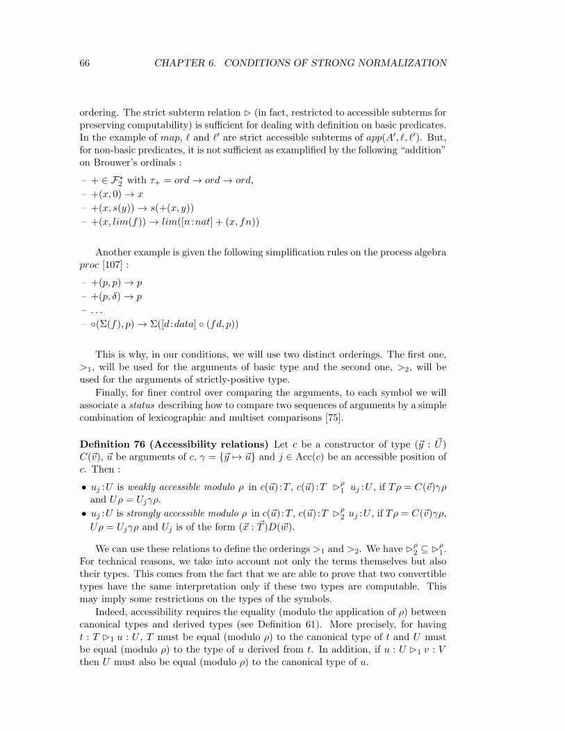
66 CHAPTER 6. CONDITIONS OF STRONG NORMALIZATION
ordering. The strict subterm relation ✄ (in fact, restricted to accessible subterms forpreserving computability) is sufficient for dealing with definition on basic predicates.In the example of map, ℓ and ℓ′ are strict accessible subterms of app(A′, ℓ, ℓ′). But,for non-basic predicates, it is not sufficient as examplified by the following “addition”on Brouwer’s ordinals :
– + ∈ F⋆2 with τ+ = ord→ ord→ ord,
– +(x, 0)→ x
– +(x, s(y))→ s(+(x, y))
– +(x, lim(f))→ lim([n :nat] + (x, fn))
Another example is given the following simplification rules on the process algebraproc [107] :
– +(p, p)→ p
– +(p, δ)→ p
– . . .
– ◦(Σ(f), p)→ Σ([d :data] ◦ (fd, p))
This is why, in our conditions, we will use two distinct orderings. The first one,>1, will be used for the arguments of basic type and the second one, >2, will beused for the arguments of strictly-positive type.
Finally, for finer control over comparing the arguments, to each symbol we willassociate a status describing how to compare two sequences of arguments by a simplecombination of lexicographic and multiset comparisons [75].
Definition 76 (Accessibility relations) Let c be a constructor of type (~y : ~U)C(~v), ~u be arguments of c, γ = {~y 7→ ~u} and j ∈ Acc(c) be an accessible position ofc. Then :
• uj :U is weakly accessible modulo ρ in c(~u) :T , c(~u) :T ✄ρ1 uj :U , if Tρ = C(~v)γρ
and Uρ = Ujγρ.
• uj :U is strongly accessible modulo ρ in c(~u) :T , c(~u) :T ✄ρ2 uj :U , if Tρ = C(~v)γρ,
Uρ = Ujγρ and Uj is of the form (~x : ~T )D(~w).
We can use these relations to define the orderings >1 and >2. We have ✄ρ2 ⊆ ✄
ρ1.
For technical reasons, we take into account not only the terms themselves but alsotheir types. This comes from the fact that we are able to prove that two convertibletypes have the same interpretation only if these two types are computable. Thismay imply some restrictions on the types of the symbols.
Indeed, accessibility requires the equality (modulo the application of ρ) betweencanonical types and derived types (see Definition 61). More precisely, for havingt : T ✄1 u : U , T must be equal (modulo ρ) to the canonical type of t and U mustbe equal (modulo ρ) to the type of u derived from t. In addition, if u : U ✄1 v : Vthen U must also be equal (modulo ρ) to the canonical type of u.
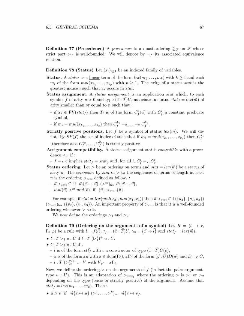
6.3. GENERAL SCHEMA 67
Definition 77 (Precedence) A precedence is a quasi-ordering ≥F on F whosestrict part >F is well-founded. We will denote by =F its associated equivalencerelation.
Definition 78 (Status) Let (xi)i≥1 be an indexed family of variables.
Status. A status is a linear term of the form lex(m1, . . . ,mk) with k ≥ 1 and eachmi of the form mul(xk1 , . . . , xkp) with p ≥ 1. The arity of a status stat is thegreatest indice i such that xi occurs in stat.
Status assignment. A status assignment is an application stat which, to eachsymbol f of arity n > 0 and type (~x : ~T )U , associates a status statf = lex(~m) ofarity smaller than or equal to n such that :
– if xi ∈ FV(statf ) then Ti is of the form Cif (~u) with Ci
f a constant predicatesymbol,
– if mi = mul(xk1 , . . . , xkp) then Ck1f =C . . . =C C
kpf .
Strictly positive positions. Let f be a symbol of status lex(~m). We will de-note by SP (f) the set of indices i such that if mi = mul(xk1 , . . . , xkp) then Ck1
f
(therefore also Ck2f , . . . , C
kpf ) is strictly positive.
Assignment compatibility. A status assignment stat is compatible with a prece-dence ≥F if :
– f =F g implies statf = statg and, for all i, Cif =F Ci
g.
Status ordering. Let > be an ordering on terms and stat = lex(~m) be a status ofarity n. The extension by stat of > to the sequences of terms of length at leastn is the ordering >stat defined as follows :
– ~u >stat ~v if ~m{~x 7→ ~u} (>m)lex ~m{~x 7→ ~v},
– mul(~u) >m mul(~v) if {~u} >mul {~v}.
For example, if stat = lex(mul(x2),mul(x1, x3)) then ~u >stat ~v if ({u2}, {u1, u3})(>mul)lex ({v2}, {v1, v3}). An important property of >stat is that it is a well-foundedordering whenever > so is.
We now define the orderings >1 and >2.
Definition 79 (Ordering on the arguments of a symbol) Let R = (l → r,Γ0, ρ) be a rule with l = f(~l), τf = (~x : ~T )U , γ0 = {~x 7→ ~l} and statf = lex(~m).
• t : T >1 u : U if t : T (✄ρ1)
+ u : U .
• t : T >2 u : U if :
– t is of the form c(~t) with c a constructor of type (~x : ~T )C(~v),
– u is of the form x~u with x ∈ dom(Γ0), xΓ0 of the form (~y : ~U)D(~w) and D =C C,
– t : T (✄ρ2)
+ x : V with V ρ = xΓ0.
Now, we define the ordering > on the arguments of f (in fact the pairs argument-type u : U). This is an adaptation of >statf where the ordering > is >1 or >2
depending on the type (basic or strictly positive) of the argument. Assume thatstatf = lex(m1, . . . ,mk). Then :
• ~u > ~v if ~m{~x 7→ ~u} (>1, . . . , >k)lex ~m{~x 7→ ~v},
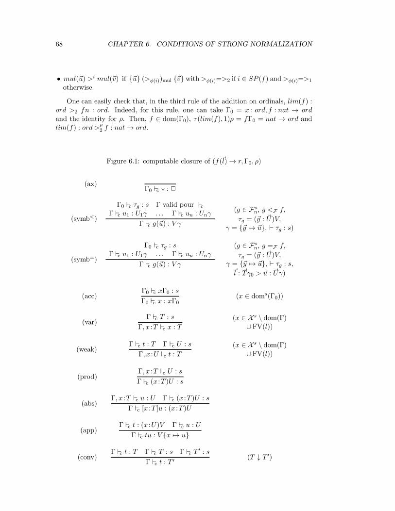
68 CHAPTER 6. CONDITIONS OF STRONG NORMALIZATION
• mul(~u) >i mul(~v) if {~u} (>φ(i))mul {~v} with>φ(i)=>2 if i ∈ SP (f) and>φ(i)=>1
otherwise.
One can easily check that, in the third rule of the addition on ordinals, lim(f) :ord >2 fn : ord. Indeed, for this rule, one can take Γ0 = x : ord, f : nat → ordand the identity for ρ. Then, f ∈ dom(Γ0), τ(lim(f), 1)ρ = fΓ0 = nat → ord andlim(f) : ord✄ρ
2 f : nat→ ord.
Figure 6.1: computable closure of (f(~l)→ r,Γ0, ρ)
(ax)Γ0 ⊢c ⋆ : ✷
(symb<)
Γ0 ⊢c τg : s Γ valid pour ⊢cΓ ⊢c u1 : U1γ . . . Γ ⊢c un : Unγ
Γ ⊢c g(~u) : V γ
(g ∈ Fsn, g <F f,
τg = (~y : ~U)V,γ = {~y 7→ ~u}, ⊢ τg : s)
(symb=)
Γ0 ⊢c τg : sΓ ⊢c u1 : U1γ . . . Γ ⊢c un : Unγ
Γ ⊢c g(~u) : V γ
(g ∈ Fsn, g =F f,
τg = (~y : ~U)V,γ = {~y 7→ ~u}, ⊢ τg : s,~l : ~Tγ0 > ~u : ~Uγ)
(acc)Γ0 ⊢c xΓ0 : s
Γ0 ⊢c x : xΓ0(x ∈ doms(Γ0))
(var)Γ ⊢c T : s
Γ, x :T ⊢c x : T
(x ∈ X s \ dom(Γ)∪FV(l))
(weak)Γ ⊢c t : T Γ ⊢c U : s
Γ, x :U ⊢c t : T
(x ∈ X s \ dom(Γ)∪FV(l))
(prod)Γ, x :T ⊢c U : s
Γ ⊢c (x :T )U : s
(abs)Γ, x :T ⊢c u : U Γ ⊢c (x :T )U : s
Γ ⊢c [x :T ]u : (x :T )U
(app)Γ ⊢c t : (x :U)V Γ ⊢c u : U
Γ ⊢c tu : V {x 7→ u}
(conv)Γ ⊢c t : T Γ ⊢c T : s Γ ⊢c T
′ : s
Γ ⊢c t : T ′(T ↓ T ′)

6.3. GENERAL SCHEMA 69
Definition 80 (Computable closure) Let R = (l → r,Γ0, ρ) be a rule with l =f(~l), τf = (~x : ~T )U and γ0 = {~x 7→ ~l}. The computable closure of R w.r.t. aprecedence ≥F and a status assignment stat compatible with ≥F is the smallestrelation ⊢c⊆ E × T × T defined by the inference rules of Figure 6.1. We will denoteby ⊢<c the restriction of ⊢c to the rules distinct from (symb=)
One can easily check that if Γ ⊢c t : T then Γ = Γ0,Γ′. And also that ⊢c⊆⊢s and
⊢<c ⊆⊢f .It is important to note that the computable closure can easily be extended by
adding new inference rules. For preserving the strong normalization, it suffices tocomplete the proof of Theorem 146 where we prove that the rules of the computableclosure indeed preserve the computability.
Definition 81 (Well-formed rule) Let R = (l→ r,Γ0, ρ) be a rule with l = f(~l),τf = (~x : ~T )U and γ0 = {~x 7→ ~l}. The rule R is well-formed if :
– Γ0 ⊢ lρ : Uγ0ρ,
– for all x ∈ dom(Γ0), there exists i such that li : Tiγ0 (✄ρ1)
∗ x : xΓ0,
– dom(ρ) ∩ dom(Γ0) = ∅.
For example, consider the rule :
appn(p, consn(x, n, ℓ), n′, ℓ′)→ consn(x, n+ n′, appn(n, ℓ, n′, ℓ′))
with Γ0 = x :T, n :nat, ℓ : listn(n), n′ :nat, ℓ′ : listn(n′) and ρ = {p 7→ s(n)}. We haveΓ0 ⊢ lρ : listn(p + n′)ρ. For x, we have consn(x, n, ℓ) : listn(p) ✄ρ
1 x : T . One caneasily check that the conditions are also satisfied for the other variables.
Definition 82 (Recursive system) Let R = (l→ r,Γ0, ρ) be a rule with l = f(~l),τf = (~x : ~T )U and γ0 = {~x 7→ ~l}. The rule R satisfies the General Schema w.r.t. aprecedence ≥F and a status assignment stat compatible with ≥F if R is well-formedand Γ0 ⊢c r : Uγ0ρ.
A set of rules R is recursive if there exists a precedence ≥F and a status as-signment stat compatible with ≥F for which every rule of R satisfies the GeneralSchema w.r.t. ≥F and stat.
Remark 83 (Decidability) A priori , because of the rule (conv) and of the condi-tion ⊢ τg : s for the rules (symb<) and (symb=), the relation ⊢c may be undecidable.On the other hand, if we assume ⊢ τg : s and restrict the rule (conv) to a confluentand strongly normalizing fragment of → then ⊢c becomes decidable (with an algo-rithm similar to the one for ⊢). In practice, the symbols and the rules are oftenadded one after the other (or by groups, but the argument can be generalized).
Let (F ,R) be a confluent and strongly normalizing system, f /∈ F and Rf a setof rules defining f and whose symbols belong to F ′ = F ∪{f}. Then (F ′,R) is alsoconfluent and strongly normalizing. Thus we can check that the rules of Rf satisfythe General Schema with the rule (conv) restricted to the case where T ↓βR T ′. Thisdoes not seem a big restriction : it would be surprising that the typing of a rulerequires the use of the rule itself!

70 CHAPTER 6. CONDITIONS OF STRONG NORMALIZATION
Before to give a detailed example, we are going to show several properties of ⊢c.Indeed, to show Γ0 ⊢c r : Uγ0ρ, knowing that by (S3) we have Γ0 ⊢ r : Uγ0ρ, onecan wonder whether it is possible to transform a derivation of Γ0 ⊢ r : Uγ0ρ into aderivation of Γ0 ⊢c r : Uγ0ρ. The best thing would be that it is sufficient that thesymbols in r are smaller than f and that the recursive calls are made on smallerarguments. We prove hereafter that it is sufficient when there is no recursive call.
Definition 84 A rule l→ r is compatible with ≥F if all the symbols in r are smallerthan or equivalent to l. A set of rule R is compatible with ≥F if every rule of R iscompatible with ≥F .
Lemma 85 Assume that R and τ are compatible with ≥F . Let Γ be an environ-ment with variables distinct from those of Γ0. If Γ ⊢f t : T then Γ0,Γ ⊢
<c t : T .
Proof. By induction on Γ ⊢f t : T . �
Lemma 86 (Substitution for ⊢c) If Γ0,Γ ⊢<c t : T and θ : Γ0,Γ → Γ0,Γ
′ in ⊢c(resp. in ⊢<c ) then Γ0,Γ
′ ⊢c tθ : Tθ (resp. Γ0,Γ′ ⊢<c tθ : Tθ).
Proof. By induction on Γ0,Γ ⊢<c t : T . �
Lemma 87 If R and τ are compatible with ≥F , → is confluent and the symbols ofΓ0 are strictly smaller than f then, for all x ∈ doms(Γ0), Γ0 ⊢
<c xΓ0 : s.
Proof. Assume that Γ0 = ~y : ~U and that yi is of sort si. We show by inductionon i that, for all j ≤ i, Γ0 ⊢
<c Uj : sj . If i = 0, this is immediate. So, assume that
i > 0. By induction hypothesis, for all j < i, Γ0 ⊢<c Uj : sj. So, we are left to show
that Γ0 ⊢<c Ui : si.
Let Γ = y1 : U1, . . . , yi−1 : Ui−1, ~z be i − 1 fresh variables, θ = {~y 7→ ~z},θ′ = {~z 7→ ~y} and Γ′ = ~z : ~Uθ. By (S3), Γ0 is valid. So, by the EnvironmentLemma, Γ ⊢ Ui : si. Since → is confluent and the symbols in Γ are strictly smallerthan f , by Lemma 54, Γ ⊢f Ui : si. By Replacement, Γ′ ⊢f Uiθ : si. Therefore, byLemma 85, Γ0,Γ
′ ⊢<c Uiθ : si.
Now we show that θ′ : Γ0,Γ′ → Γ0 in ⊢<c . For this, it is sufficient to show that,
for all j < i, Γ0 ⊢<c zjθ
′ : Ujθθ′, that is, Γ0 ⊢
<c yj : Uj . By induction hypothesis, for
all j < i, Γ0 ⊢<c Uj : sj . Thus, by (acc), Γ0 ⊢
<c yj : Uj . So, θ′ : Γ′ → Γ0 in ⊢<c and,
by Lemma 86, Γ0 ⊢<c Ui : si. �
Lemma 88 If R and τ are compatible with ≥F , → is confluent and Γ0,Γ ⊢f t : Tthen Γ0,Γ ⊢
<c t : T .
Proof. By induction on the size of Γ. Assume that Γ0,Γ = ~y : ~U . Let ~z be|~y| fresh variables, θ = {~y 7→ ~z}, θ′ = {~z 7→ ~y} and ∆ = ~z : ~Uθ. By Replacement,∆ ⊢f tθ : Tθ. By Lemma 85, Γ0,∆ ⊢<c tθ : Tθ. Now we show that θ′ : Γ0,∆→ Γ0,Γin ⊢<c in order to conclude with Lemma 86.
We must show that, for all x ∈ dom(Γ0,∆), Γ0,Γ ⊢<c xθ′ : x(Γ0,∆). If x ∈
dom(Γ0) then we have to show that Γ0,Γ ⊢<c x : xΓ0, and if x = zi ∈ dom(∆)
then we have to show that Γ0,Γ ⊢<c yi : Ui. So, it is sufficient to show that Γ0,Γ

6.4. STRONG NORMALIZATION CONDITIONS 71
is valid in ⊢<c . If Γ is empty, this is immediate since, by Lemma 87, Γ0 is valid in⊢<c . Assume now that Γ = Γ′, y : U . Then, ∆ = ∆′, z : Uθ. By the EnvironmentLemma, Γ0,Γ
′ ⊢f U : s. By induction hypothesis, Γ0,Γ′ ⊢<c U : s. Therefore, by
(var), Γ0,Γ ⊢<c y : U and Γ0,Γ is valid in ⊢<c . �
A particular but useful case is :
Corollary 89 If R and τ are compatible with ≥F and → is confluent then, for allg ≤F f , if ⊢ τg : s then Γ0 ⊢
<c τg : s.
Proof. Since τ is compatible with ≥F and → is confluent, by Lemma 54,⊢f τg : s. Thus, by Lemma 85, Γ0 ⊢
<c τg : s. �
Now, we can detail an example. Let us consider the rule :
appn(p, consn(x, n, ℓ), n′, ℓ′)→ consn(x, n+ n′, appn(n, ℓ, n′, ℓ′))
with Γ0 = x :T, n :nat, ℓ : listn(n), n′ :nat, ℓ′ : listn(n′) and ρ = {p 7→ s(n)}. We takestatappn = lex(mul(x2)); appn >F consn,+; consn >F T and + >F s, 0 >F nat.We have already seen that this rule is well formed. Let us show that Γ0 ⊢c r :listn(s(n)). We have R and τ compatible with ≥F .
For applying (symb<), we must show ⊢ τconsn : ⋆, Γ0 ⊢c τconsn : ⋆, Γ0 ⊢c x : T ,Γ0 ⊢c n + n′ : nat and Γ0 ⊢c appn(n, ℓ, n
′, ℓ′) : listn(n+ n′). It is easy to check that⊢ τconsn : ⋆. Then, by Lemma 89, we deduce that Γ0 ⊢c τconsn : ⋆. The assertionsΓ0 ⊢c x : T and Γ0 ⊢c n + n′ : nat come from Lemma 88. We are left to show thatΓ0 ⊢c appn(n, ℓ, n
′, ℓ′) : listn(n+ n′).
For applying (symb=), we must show that ⊢ τappn : ⋆, Γ0 ⊢c τappn : ⋆, Γ0 ⊢cn : nat, Γ0 ⊢c ℓ : listn(n), Γ0 ⊢c n
′ : nat, Γ0 ⊢c ℓ′ : listn(n′) and consn(x, n, ℓ) :
listn(s(n)) >1 ℓ : listn(n). It is easy to check that ⊢ τappn : ⋆. Then, by Lemma 89,we deduce that Γ0 ⊢c τappn : ⋆. The assertion consn(x, n, ℓ) : listn(p) >1 ℓ : listn(n)has already be shown for proving that the rule is well formed. The other assertionscome from Lemma 88.
6.4 Strong normalization conditions
Definition 90 (Rewrite systems) Let G be a set of symbols. The rewrite system
(G,RG) is :
• of first-order if :
– G is made of predicate symbols of maximal arity or of constructors of primitivepredicates,
– the rules of RG have an algebraic right hand-side;
• non-duplicating if, for all rule of RG , no variable has more occurrences in the righthand-side than in the left hand-side;
• primitive if all the rules of RG have a right hand-side of the form [~x : ~T ]g(~u)~vwith g a symbol of G or a primitive predicate;
• simple if there is no critical pairs between cRG and R :
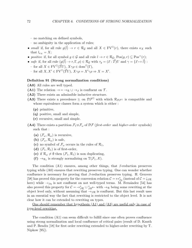
72 CHAPTER 6. CONDITIONS OF STRONG NORMALIZATION
– no matching on defined symbols,
– no ambiguity in the application of rules;
• small if, for all rule g(~l) → r ∈ RG and all X ∈ FV✷(r), there exists κX suchthat lκX
= X;
• positive if, for all symbol g ∈ G and all rule l → r ∈ RG , Pos(g, r) ⊆ Pos+(r);
• safe if, for all rule (g(~l)→ r,Γ, ρ) ∈ RG with τg = (~x : ~T )U and γ = {~x 7→ ~l} :
– for all X ∈ FV✷(~TU), Xγρ ∈ dom✷(Γ),
– for all X,X ′ ∈ FV✷(~TU), Xγρ = X ′γρ⇒ X = X ′.
Definition 91 (Strong normalization conditions)
(A0) All rules are well typed.
(A1) The relation →=→R ∪ →β is confluent on T .
(A2) There exists an admissible inductive structure.
(A3) There exists a precedence � on DF✷ with which RDF✷ is compatible andwhose equivalence classes form a system which is either :
(p) primitive,
(q) positive, small and simple,
(r) recursive, small and simple.
(A4) There exists a partition F1⊎Fω of DF (first-order and higher-order symbols)such that :
(a) (Fω,Rω) is recursive,
(b) (Fω,Rω) is safe,
(c) no symbol of Fω occurs in the rules of R1,
(d) (F1,R1) is of first-order,
(e) if Rω 6= ∅ then (F1,R1) is non duplicating,
(f) →R1is strongly normalizing on T(F1,X ).
The condition (A1) ensures, among other things, that β-reduction preservestyping while (A0) ensures that rewriting preserves typing. One can wonder whetherconfluence is necessary for proving that β-reduction preserves typing. H. Geuvers[58] has proved this property for the conversion relation C =↔∗
βη (instead of C = ↓βRhere) while →βη is not confluent on not well-typed terms. M. Fernandez [54] hasalso proved this property for C =→∗
βR ∪∗βR← with→R being some rewriting at the
object level only, without assuming that →βR is confluent. But this last result usesin an essential way the fact that rewriting is restricted to the object level. It is notclear how it can be extended to rewriting on types.
One should remember that hypothesis (A1) and (A3) are useful only in case oftype-level rewriting.
The condition (A1) can seem difficult to fulfill since one often proves confluenceusing strong normalization and local confluence of critical pairs (result of D. Knuthand P. Bendix [18] for first order rewriting extended to higher-order rewriting by T.Nipkow [95]).

6.4. STRONG NORMALIZATION CONDITIONS 73
We know that →β is confluent and that there is no critical pair between R andthe β-reduction since the left hand-sides of the rules of R are algebraic.
F. Muller [92] has shown that, in this case, if →R is confluent and all the rulesof R are left-linear, then →R ∪ →β is confluent. Thus, the possibility we haveintroduced, of linearizing some rules (substitution ρ) while keeping subject reduction,appears to be very useful.
In the case of left-linear rules, and assuming that →R1is strongly normalizing
as it is required in (f), how can we prove that → is confluent? In the case where→R1
is non duplicating if Rω 6= ∅, we show in Theorem 144 that →R1∪ →Rω is
strongly normalizing. Therefore, it suffices to check that the critical pairs of R areconfluent (without using any β-reduction).
In (A4), in the case where Rω 6= ∅, we require that the rules of R1 are non-duplicating. Indeed, with first-order rewriting already, strong normalization is nota modular property [114], even with confluent systems [53]. On the other hand, itis modular for disjoint and non duplicating systems [104]. Here, R1 and Rω arenot disjoint but hierarchically defined : by (c), no symbol of Fω occurs in the rulesof R1. In [43], N. Dershowitz gathers many results on the modularity of strongnormalization for first-order rewrite systems, especially for hierarchically definedsystems. It would be very interesting to study the modularity of strong normalizationin the case of higher-order rewriting and, in particular, other conditions than non-duplication which, for example, does not allow us to accept the following definition :
0/y → 0s(x)/y → s((x− y)/y)
0− y → 0s(x)− 0 → s(x)
s(x)− s(y) → x− y
This system is a duplicating first-order system not satisfying the General Schema:it can be put neither in R1 nor in Rω. E. Gimenez [61] can deal with this exampleby using the fact that the result of x− y is smaller than s(x).
In (A3), the smallness condition for recursive and positive systems is equivalentin the Calculus of Inductive Constructions to the restriction of strong elimination to“small” inductive types, that is, the types whose constructors have no other predicatearguments than the ones of their type. For example, the type list of polymorphiclist is small since, in (A :⋆)A→ list(A)→ list(A), the type of its constructor cons,A is an argument of list. On the other hand, a type T having a constructor c oftype ⋆→ T is not small. So, we cannot define a function f of type T → ⋆ with therule f(c(A)) → A. Such a rule is not small and does not form a primitive systemeither. In some sense, primitive systems can always be considered as small systemssince they contain no projection and primitive predicate symbols have no predicateargument.

74 CHAPTER 6. CONDITIONS OF STRONG NORMALIZATION
Finally, in (A4), the safeness condition for higher-order symbols means that onecannot do matching or equality tests on predicate arguments that are necessaryfor typing other arguments. In her extension of HORPO [76] to the Calculus ofConstructions, D. Walukiewicz [118] requires a similar condition. She gives several(pathological) examples of non termination because of non-safeness like J(A,A, a)→a with J : (A : ⋆)(B : ⋆)B → A or J(A,A, a, b) → b with J : (A : ⋆)(B : ⋆)A → B →A. On the other hand, the rule map(A,A, [x : A]x, ℓ) → ℓ, which does not seemproblematic, does not satisfy the safeness condition either (note that the left hand-side if not algebraic).
We can now state our main result :
THEOREM : If a CAC satisfies the conditions of Definition 91 then its reduc-tion relation →=→R ∪ →β preserves typing and is strongly normalizing.
The proof of this theorem is the subject of Chapter 8. This generalizes the resultsof M. Fernandez [54] and of J.-P. Jouannaud, M. Okada and myself [22]. In Chap-ter 7, we give several important examples of CAC’s satisfying these conditions : animportant subsystem with strong elimination of the Calculus of Inductive Construc-tions (CIC) and the Natural Deduction Modulo (NDM) a large class of equationaltheories.
On the other hand, these conditions do not capture the decision procedure forclassical propositional tautologies of Figure 1.3. Let us see why :
– We did not consider rewriting modulo associativity and commutativity.
– Since the system is not left-linear, we do not know how to prove the confluenceof its combination with β.
– The system is not primitive since there are projections (P xor⊥ → P ). It isrecursive (and positive also) and small. Unfortunately, it is not simple.
Rewriting modulo AC does not seem to be a difficult extension, except perhapsin the case of type-level rewriting. On the other hand, confluence and simplicityare problems which seem difficult but we expect to solve them in the future. InSection 9, we give other directions for future work but these three problems arecertainly the most important ones.
From strong normalization, we can deduce the decidability of the typing relation,which is the essential property on which proof assistants like Coq [112] and LEGO[82] are based.
Theorem 92 (Decidability of ⊢) Let Γ be a valid environment and T be ✷ ora term typable in Γ. In a CAC satisfying the conditions of Definition 91, checkingwhether a term t is of type T in Γ is decidable.
Proof. Since Γ is valid, it is possible to say whether t is typable and, if so, it ispossible to infer a type T ′ for t. Since types are convertible, it suffices to check that
6.4. STRONG NORMALIZATION CONDITIONS 75
T and T ′ have the same normal form. The reader is invited to look at [35, 11] formore details. �
Remark 93 (Logical consistency)In the pure Calculus of Constructions (CC), it is easy to check that, in the empty
environment, no normal proof of ⊥ = (P : ⋆)P can exist [10]. Therefore, for CC,strong normalization is sufficient for proving the logical consistency.
On the other hand, in a CAC, the situation is not so simple. From a logicalpoint of view, having symbols is equivalent to working in a non empty environment.Therefore, it is possible that symbols and rules allow one to build a normal proofof ⊥. In [106], J. Seldin shows the logical consistency of the “strongly consistent”environments 3 by syntactical means. However, for proving the consistency of morecomplex environments, it may be necessary to use semantic methods.
3An environment Γ is strongly consistent if, for all x ∈ dom(Γ), either xΓ is a predicate type, orxΓ is β-equivalent to a term of the form y~t.

76 CHAPTER 6. CONDITIONS OF STRONG NORMALIZATION
Chapter 7
Examples of CAC’s
7.1 Calculus of Inductive Constructions (CIC)
We are going to show that our conditions of strong normalization capture mostof the Calculus of Inductive Constructions (CIC) of B. Werner [119] which is thebasis of the proof assistant Coq [112]. But, since CIC is expressed in a formalismdifferent from ours, we need to translate CIC into our formalism in order to checkour conditions. It is a little bit long and painful but not very difficult.
In order to type the strong elimination schema in a polymorphic way, which isnot possible in the usual Calculus of Constructions, B. Werner uses a slightly moregeneral type system with the sorts S = {⋆,✷,△}, the axioms A = {(⋆,✷), (✷,△)}and the rules B = {(s1, s2, s3) ∈ S
3 | s1 ∈ {⋆,✷}, s2 = s3} (in fact, he denotes ⋆ bySet, ✷ by Type and △ by Extern).
Then he adds terms for representing inductive types, their constructors and thedefinitions by recursion on these types :
• inductive types : An inductive type is denoted by I = Ind(X :A){~C} where theCi’s are the types of the constructors of I. For example, Nat = Ind(X :⋆){X,X →X} represents the type of natural numbers (in fact, any type isomorphic to thetype of natural numbers). The term A must be of the form (~x : ~A)⋆ and the Ci’sof the form (~z : ~B)X~m with X /∈ FV(~m). Furthermore, the inductive types mustbe strictly positive. In CIC, this means that, if Ci = (~z : ~B)X~m then, for all j,either X does not appear in Bj , or Bj is of the form (~y : ~D)X~q and X does not
appear neither in ~D nor in ~q.
• constructors : The i-th constructor of an inductive type I is denoted byConstr(i, I). For example, Constr(1, Nat) represents zero and Constr(2, Nat)represents the successor function.
• definitions by recursion : A definition by recursion on an inductive type I isdenoted by Elim(I,Q,~a, c) where Q is the type of the result, ~a the arguments ofI and c a term of type I~a. The strong elimination (that is, in the case where Qis a predicate type) is restricted to “small” inductive types, that is, the typeswhose constructors do not have predicate arguments that their type do not have.More precisely, an inductive type I = Ind(X : A){~C} is small if all the types
77
78 CHAPTER 7. EXAMPLES OF CAC’S
of its constructors are small and a constructor type C = (~z : ~B)X~m is small
if {~z} ∩ X✷ = ∅ (this means that the predicate arguments must be part of theenvironment in which they are typed; they cannot be part of ~C).
For defining the reduction relation associated with Elim, called ι-reductionand denoted →ι, and the typing rules of Elim (see Figure 7.1), it is necessary tointroduce a few definitions.
Let C be a constructor type. We define ∆{I,X,C,Q, c} as follows :
– ∆{I,X,X ~m,Q, c} = Q~mc
– ∆{I,X, (z :B)D,Q, c} = (z :B)∆{I,X,D,Q, cz} if X /∈ FV(B)
– ∆{I,X, (z :B)D,Q, c} = (z :B{X 7→I})((~y : ~D)Q~q (z~y))→ ∆{I,X,D,Q, cz}if B = (~y : ~D)X~q
The ι-reduction is defined by the rule :
Elim(I,Q, ~x,Constr(i, I ′) ~z){~f} →ι ∆[I,X,Ci, fi, FunElim(I,Q, ~f )] ~z
where I = Ind(X :A){~C}, FunElim(I,Q, ~f) = [~x : ~A][y :I~x]Elim(I,Q, ~x, y){~f} and∆[I,X,C, f, F ] is defined as follows :
– ∆[I,X,X ~m, f, F ] = f
– ∆[I,X, (z :B)D, f, F ] = [z :B]∆[I,X,D, fz, F ] if X /∈ FV(B)
– ∆[I,X, (z :B)D, f, F ] = [z :B{X 7→I}]∆[I,X,D, fz [~y : ~D](F~q (z~y)), F ]if B = (~y : ~D)X~q
Finally, in the type conversion rule (conv), in addition to β-reduction and ι-reduction, B. Werner considers η-reduction : [x :T ]ux→η u if x /∈ FV(u). Since→βη
is not confluent on badly typed terms1, to consider η-reduction creates importantdifficulties [58]. Therefore, since our condition (A1) cannot be satisfied with η-reduction, we cannot consider η-reduction. To find a condition weaker than (A1)that would be satisfied even with η-reduction is a problem that we have temporallyleft open.
The ι-reduction as defined above introduces many β-redexes and the recursivecalls on Elim are made on bound variables which must be instanciated by strictsubterms (or terms of smaller order in case of a strictly positive inductive type).So, on one hand, from a practical point of view, this is not very efficient sincethese instanciations could be done immediately after the ι-reduction, and on theother hand, the General Schema cannot directly deal with recursive calls on boundvariables, even though these variables must be instanciated with smaller terms.
This is why we are not going to show the strong normalization of the relation→βι but of the relation →βι′ where one step of →ι′ corresponds to a ι-reductionfollowed by as many β-reductions as necessary for erasing the β-redexes introducedby the ι-reduction. Note that this is indeed this reduction relation which is actuallyimplemented in the Coq system [112].
Definition 94 (ι′-reduction) The ι′-reduction is the reduction relation defined bythe rule :
1Remark due to R. Nederpelt [93] : [x :A]x β← [x :A]([y :B]y x)→η [y :B]y.
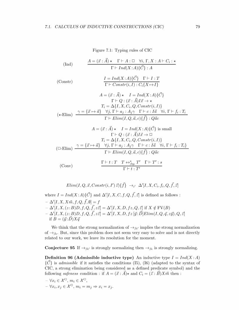
7.1. CALCULUS OF INDUCTIVE CONSTRUCTIONS (CIC) 79
Figure 7.1: Typing rules of CIC
(Ind)A = (~x : ~A) ⋆ Γ ⊢ A : ✷ ∀i, Γ,X : A ⊢ Ci : ⋆
Γ ⊢ Ind(X :A){~C} : A
(Constr)I = Ind(X :A){~C} Γ ⊢ I : T
Γ ⊢ Constr(i, I) : Ci{X 7→I}
(⋆-Elim)
A = (~x : ~A) ⋆ I = Ind(X :A){~C}
Γ ⊢ Q : (~x : ~A)I~x→ ⋆Ti = ∆{I,X,Ci, Q,Constr(i, I)}
γ = {~x 7→ ~a} ∀j, Γ ⊢ aj : Ajγ Γ ⊢ c : I~a ∀i, Γ ⊢ fi : Ti
Γ ⊢ Elim(I,Q,~a, c){~f} : Q~ac
(✷-Elim)
A = (~x : ~A) ⋆ I = Ind(X :A){~C} is small
Γ ⊢ Q : (~x : ~A)I~x→ ✷
Ti = ∆{I,X,Ci, Q,Constr(i, I)}γ = {~x 7→ ~a} ∀j, Γ ⊢ aj : Ajγ Γ ⊢ c : I~a ∀i, Γ ⊢ fi : Ti}
Γ ⊢ Elim(I,Q,~a, c){~f} : Q~ac
(Conv)Γ ⊢ t : T T ↔∗
βηι T′ Γ ⊢ T ′ : s
Γ ⊢ t : T ′
Elim(I,Q, ~x,Constr(i, I ′) ~z){~f} →ι′ ∆′[I,X,Ci, fi, Q, ~f , ~z]
where I = Ind(X :A){~C} and ∆′[I,X,C, f,Q, ~f , ~z] is defined as follows :
– ∆′[I,X,X ~m, f,Q, ~f , ∅] = f
– ∆′[I,X, (z :B)D, f,Q, ~f , z~z] = ∆′[I,X,D, fz,Q, ~z] if X /∈ FV(B)
– ∆′[I,X, (z :B)D, f,Q, ~f , z~z] = ∆′[I,X,D, fz [~y : ~D]Elim(I,Q, ~q, z~y), Q, ~z]if B = (~y : ~D)X~q
We think that the strong normalization of→βι′ implies the strong normalizationof →βι. But, since this problem does not seem very easy to solve and is not directlyrelated to our work, we leave its resolution for the moment.
Conjecture 95 If →βι′ is strongly normalizing then →βι is strongly normalizing.
Definition 96 (Admissible inductive type) An inductive type I = Ind(X :A){~C} is admissible if it satisfies the conditions (I5), (I6) (adapted to the syntax ofCIC, a strong elimination being considered as a defined predicate symbol) and thefollowing safeness condition : if A = (~x : ~A)⋆ and Ci = (~z : ~B)X~m then :
– ∀xi ∈ X✷, mi ∈ X
✷,
– ∀xi, xj ∈ X✷, mi = mj ⇒ xi = xj .
80 CHAPTER 7. EXAMPLES OF CAC’S
Definition 97 (CIC−) The sub-system of CIC that we are going to consider,CIC−, can be obtained by applying the following restrictions :
• We exclude any use of the sort△ in order to stay in the Calculus of Constructions.
• In the rule (Ind), instead of requiring I = Ind(X :A){~C} to be typable in any en-vironment Γ, we require I to be typable in the empty environment since, in CAC,the types of the symbols must be typable in the empty environment. Moreover,we require I to be admissible and in normal form.
The restriction to the empty environment is not a real restriction since anytype I = Ind(X :A){~C} typable in an environment Γ = ~y : ~U can be replacedby a type I ′ = Ind(X ′ :A′){~C ′} typable in the empty environment : it sufficesto take A′ = (~y : ~U)A, C ′
i = (~y : ~U)Ci{X 7→ X ′~y} and to replace I by I ′~y andConstr(i, I) by Constr(i, I ′)~y.
But we need to adapt the definition of small constructor type as follows : aconstructor type C of an inductive type I = Ind(X :A){~C} with A = (~x : ~A)⋆ issmall if it is of the form (~x : ~A)(~z : ~B)X~m with {~z} ∩ X✷ = ∅.
• In the rule (⋆-Elim), instead of requiring Q to be typable in any environment Γ,we require Q to be typable in the empty environment. Moreover, we explicitlyrequire I and Ti = ∆{I,X,Ci, Q,Constr(i, I)} to be typable.
• In the rule (✷-Elim), instead of requiring ⊢ Q : (~x : ~A)I~x→ ✷, which is not possi-ble in the Calculus of Constructions, we require Q to be of the form [~x : ~A][y :I~x]Kwith ~x : ~A, y :I~x ⊢ K : ✷ and fi to be of type Ti = ∆′{I,X,Ci, ~xy,K,Constr(i, I)}where ∆′{I,X,C, ~xy,K, c} is defined as follows :
– ∆′{I,X,X ~m, ~xy,K, c} = K{~x 7→ ~m, y 7→ c},
– if B = (~y : ~D)X~q then ∆′{I,X, (z : B)D,~xy,K, c} = (z : B{X 7→ I})((~y :~D)K{~x 7→~q, y 7→z~y})→ ∆′{I,X,D, ~xy,K, cz}.
Moreover, we require Q to be in normal form, Ti to be typable and theinductive types that occur in Q to be subterms of I. Finally, we take Γ ⊢Elim(I,Q,~a, c){~f} : K{~x 7→ ~a, y 7→ c} instead of Γ ⊢ Elim(I,Q,~a, c){~f} : Q~ac.
Requiring Q to be of the form [~x : ~A][y :I~x]K is not a real restriction since, asshown by B. Werner (Corollary 2.9 page 57 of [119]), if Γ ⊢ Q : ✷ then there existsQ′ of the form (~y : ~U)⋆ such that Q →∗
β Q′. Hence, if ⊢ Q : (~x : ~A)I~x → ✷ then
~x : ~A, y : I~x ⊢ Q~xy : ✷. Therefore, there exists Q′ of the form (~y : ~U)⋆ such thatQ~xy →∗
β Q′. Then, [~x : ~A][y : I~x]Q~xy →∗
β [~x : ~A][y : I~x]Q′ and [~x : ~A][y : I~x]Q~xy →∗η
Q. Therefore, by confluence, there exists Q′′ of the form [~x : ~A][y :I~x](~y : ~U ′)⋆ suchthat Q→∗
βη Q′′.
On the other hand, requiring the inductive types occurring in Q to be subtermsof I is a more important restriction. But it is only due to the fact that we restrictourself to the Calculus of Constructions in which it is not possible to type thestrong elimination schema in a polymorphic way (that is why B. Werner used aslightly more general PTS).
• In the rule (conv), instead of requiring T ↔∗βηι T
′, we require T ↔∗βι′ T
′ which isequivalent to T ↓βι′ T
′ since →βι′ is confluent (orthogonal CRS [79]).
We will denote by →βι′ the reduction relation of CIC−, by NF the set of CIC−
terms in normal form for →βι′ (unique by confluence), by t ↓ the normal form of t,

7.1. CALCULUS OF INDUCTIVE CONSTRUCTIONS (CIC) 81
and by ⊢ the typing relation of CIC− (see Figure 7.2).
Figure 7.2: Typing rules of CIC−
(Ind)
A = (~x : ~A)⋆ ⊢ A : ✷ ∀i, X : A ⊢ Ci : ⋆
I = Ind(X :A){~C} ∈ NF is admissible
⊢ I : A
(Constr)I = Ind(X :A){~C} Γ ⊢ I : T
Γ ⊢ Constr(i, I) : Ci{X 7→I}
(⋆-Elim)
A = (~x : ~A) ⋆ I = Ind(X :A){~C} Γ ⊢ I : T
⊢ Q : (~x : ~A)I~x→ ⋆Ti = ∆{I,X,Ci, Q,Constr(i, I)} ⊢ Ti : ⋆
γ = {~x 7→ ~a} ∀j, Γ ⊢ aj : Ajγ Γ ⊢ c : I~a ∀i, Γ ⊢ fi : Ti
Γ ⊢ Elim(I,Q,~a, c){~f} : Q~ac
(✷-Elim)
A = (~x : ~A) ⋆ I = Ind(X :A){~C}
Q = [~x : ~A][y :I~x]K ∈ NF ~x : ~A, y : I~x ⊢ K : ✷the inductive types of Q are subterms of I
Ti = ∆′{I,X,Ci, ~xy,K,Constr(i, I)} ⊢ Ti : ✷γ = {~x 7→ ~a} ∀j, Γ ⊢ aj : Ajγ Γ ⊢ c : I~a ∀i, Γ ⊢ fi : Ti
Γ ⊢ Elim(I,Q,~a, c){~f} : K{~x 7→ ~a, y 7→ c}
(Conv)Γ ⊢ t : T T ↔∗
βι′ T′ Γ ⊢ T ′ : s
Γ ⊢ t : T ′
Theorem 98 There exists a CAC Υ (with typing relation ⊢Υand reduction relation
→) satisfying the conditions of Definition 91 and a function 〈 〉 which, to a CIC−
term, associates a Υ term such that :
– if Γ ⊢ t : T then 〈Γ〉 ⊢Υ〈t〉 : 〈T 〉,
– moreover, if t→βι′ t′ then 〈t〉 →+ 〈t′〉.
Hence, →βι′ is strongly normalizing in CIC−.
Definition 99 (Translation) We define 〈t〉 on the well-typed terms, by inductionon Γ ⊢ t : T :
• Let I = Ind(X :A){~C} with A = (~x : ~A)⋆. We take 〈I〉 = [~x : 〈 ~A〉]IndI(~x) whereIndI is a symbol of type 〈A〉.
• By hypothesis, Ci = (~z : ~B)X~m. We take 〈Constr(i, I)〉 = [~z : 〈 ~B〉θ′]ConstrIi (~z)
where θ′ = {X 7→ 〈I〉}, ConstrIi is a symbol of type (~z : ~B′)IndI(〈~m〉), B′j = 〈Bj〉
if X does not occur in Bj, and B′j = (~y :〈 ~D〉)IndI(〈~q〉) if Bj = (~y : ~D)X~q.
• Let Q be a term not of the form [~x : ~A][y : I~x]K with K = (~y : ~U)⋆. Wetake 〈Elim(I,Q,~a, c){~f}〉 = WElimI(〈Q〉, 〈~a〉, 〈c〉, 〈~f〉) where WElimI is a sym-

82 CHAPTER 7. EXAMPLES OF CAC’S
bol of type (Q : (~x : 〈 ~A〉) 〈I〉~x → ⋆)(~x : 〈 ~A〉)(y : 〈I〉~x)(~f : 〈~T 〉)〈Q〉~xy and Ti =∆{I,X,Ci, Q,Constr(i, I)}.
• Let Q be a term of the form [~x : ~A][y : I~x]K with K = (~y : ~U)⋆. We take〈Elim(I,Q,~a, c){~f}〉 = SElimQ
I (〈~a〉, 〈c〉, 〈~f 〉) where SElimQ
I is a symbol of type
(~x :〈 ~A〉)(y :〈I〉~x)(~f :〈~T 〉)〈K〉, Ti = ∆′{I,X,Ci, ~xy,K,Constr(i, I)}.
• The other terms are defined recursively : 〈uv〉 = 〈u〉〈v〉, . . .
Let Υ be the CAC whose symbols are those just previously defined and whose rulesare :
WElimI(Q,~x,ConstrIi (~z),
~f) → ∆′W [I,X,Ci, fi, Q, ~f , ~z]
SElimQI (~x,Constr
Ii (~z),
~f) → ∆′S[I,X,Ci, fi, Q, ~f , ~z]
where ∆′W [I,X,C, f,Q, ~f , ~z] and ∆′
S[I,X,C, f,Q,~f , ~z] are defined as follows :
– ∆′W [I,X,X ~m, f,Q, ~f , ~z] = ∆′
S[I,X,X ~m, f,Q, ~f , ~z] = f ,
– ∆′S[I,X, (z :B)D, f,Q, ~f , z~z] = ∆′
S[I,X,D, f z,Q,~f , ~z]
and ∆′W [I,X, (z :B)D, f,Q, ~f , z~z] = ∆′
W [I,X,D, f z,Q, ~f , ~z] if X /∈ FV(B)
– ∆′S[I,X, (z : B)D, f,Q, ~f , z~z] = ∆′
S [I,X,D, f z [~y : ~D]SElimQI (~f, ~q, z~y), Q, ~f , ~z]
and ∆′W [I,X, (z :B)D, f,Q, ~f , z~z] =
∆′W [I,X,D, f z [~y : ~D]WElimI(Q, ~f, ~q, z~y), Q, ~f , ~z] if B = (~y : ~D)X~q
Since →βι′ is confluent, the β-reduction has the subject reduction property inΥ. This will be useful for proving that the translation preserves typing :
Lemma 100 If Γ ⊢ t : T then 〈Γ〉 ⊢Υ〈t〉 : 〈T 〉.
Proof. By induction on Γ ⊢ t : T .
(Ind) We have to prove that ⊢Υ〈I〉 : 〈A〉. We have 〈I〉 = [~x : 〈 ~A〉]IndI(~x) with
IndI of type 〈A〉 = (~x : 〈 ~A〉)⋆. Since ⊢ A : ✷, by induction hypothesis, we have⊢Υ〈A〉 : ✷, that is, ⊢
ΥτIndI : ✷. By inversion, we get ~x : 〈 ~A〉 ⊢
Υ⋆ : ✷. Therefore,
Γ = ~x : 〈 ~A〉 is valid and, by the Environment Lemma and (weak), for all i,Γ ⊢
Υxi : 〈Ai〉. Hence, by (symb), Γ ⊢
ΥIndI(~x) : ⋆ and, by (abs), Γ ⊢
Υ〈I〉 : 〈A〉.
(Constr) We have to prove that 〈Γ〉 ⊢Υ〈Constr(i, I)〉 : 〈Ciθ〉 where θ = {X 7→ I}.
We have Ci = (~z : ~B) X~m, 〈Constr(i, I)〉 = [~z : 〈 ~B〉θ′]ConstrIi (~z), θ′ = {X 7→
〈I〉}, ConstrIi of type (~z : ~B′)IndI(〈~m〉), B′j = 〈Bj〉 if X does not occur in Bj ,
B′j = (~y : 〈 ~D〉)IndI(〈~q〉) if Bj = (~y : ~D)X~q, 〈Ciθ〉 = 〈Ci〉θ
′ = (~z : 〈 ~B〉θ′)〈I〉〈~m〉 and
〈I〉 = (~x :〈 ~A〉)IndI(~x).Hence, 〈I〉〈~m〉 →∗
β IndI(〈~m〉). Moreover, if X does not occur in Bj then
B′j = 〈Bj〉 = 〈Bj〉θ
′. If Bj = (~y : ~D)X~q then B′j = (~y : 〈 ~D〉)IndI(〈~q〉) and
〈Bj〉θ′ = (~y :〈 ~D〉)〈I〉〈~q〉. Since, 〈I〉〈~q〉 →∗
β IndI(〈~q〉), for all j, 〈Bj〉θ′ →∗
β B′j .
Since Γ ⊢ I : T , by induction hypothesis, 〈Γ〉 ⊢Υ〈I〉 : 〈T 〉 and 〈Γ〉 is valid. By
inversion, ⊢ I : A and X : A ⊢ Ci : ⋆. By inversion again, X : A,~z : ~B ⊢ X~m : ⋆.By induction hypothesis, ⊢
Υ〈I〉 : 〈A〉 and X : 〈A〉, ~z : 〈 ~B〉 ⊢
ΥX〈~m〉 : ⋆. By
substitution, ~z : 〈 ~B〉θ′ ⊢Υ〈I〉〈~m〉 : ⋆. Therefore, ∆ = ~z : 〈 ~B〉θ′ is valid. Since
〈 ~B〉θ′ →∗β~B′, by subject reduction on the environments, ∆′ = ~z : ~B′ is also valid.
7.1. CALCULUS OF INDUCTIVE CONSTRUCTIONS (CIC) 83
Therefore, ~z : ~B′ ⊢Υ〈I〉〈~m〉 : ⋆ and, by (prod), ⊢
Υ(~z : ~B′)IndI(〈~m〉) : ⋆, that is,
⊢ΥτConstrIi
: ⋆.
By the Environment Lemma and (conv), for all j, ∆ ⊢Υzj : B′
j . Therefore,
by (symb), ∆ ⊢ΥConstrIi (~z) : IndI(〈~m〉) and, by (abs), ⊢
Υ〈Constr(i, I)〉 : (~z :
〈 ~B〉θ′)IndI(〈~m〉). Finally, by (conv) and (weak), 〈Γ〉 ⊢Υ〈Constr(i, I)〉 : 〈Ciθ〉.
(⋆-Elim) We have to prove that 〈Γ〉 ⊢Υ〈Elim(I,Q,~a, c){~f}〉 : 〈Q~ac〉. We have
〈Elim(I,Q,~a, c){~f}〉 = WElimI(〈Q〉, 〈~a〉, 〈c〉, 〈~f〉), WElimI of type (Q : 〈B〉)(~x :〈 ~A〉)(y : I~x)(~f : 〈~T 〉)〈Q〉~xy, B = (~x : ~A)I~x → ⋆, Ti = ∆{I,X,Ci, Q,Constr(i, I)}and 〈Q~ac〉 = 〈Q〉〈~a〉〈c〉. In order to apply (symb), we prove that (1) 〈Γ〉 ⊢
Υ〈Q〉 :
〈B〉, (2) 〈Γ〉 ⊢Υ〈~a〉 : 〈 ~A〉γ′, (3) 〈Γ〉 ⊢
Υ〈c〉 : 〈I〉~xγ′, (4) 〈Γ〉 ⊢
Υ〈~f〉 : 〈~T 〉γ′ and
(5) ⊢ΥτWElimI
: ⋆, where γ′ = {Q 7→ 〈Q〉, ~x 7→ 〈~a〉, y 7→ 〈c〉, ~f 7→ 〈~f〉}. First of all,note that, since Γ ⊢ c : I~a, by induction hypothesis, 〈Γ〉 ⊢
Υ〈c〉 : 〈I~a〉 and 〈Γ〉 is
valid.
(1) Since ⊢ Q : B, by induction hypothesis, ⊢Υ〈Q〉 : 〈B〉. Therefore, by weakening,
〈Γ〉 ⊢Υ〈Q〉 : 〈B〉.
(2) Since Γ ⊢ aj : Ajγ, by induction hypothesis, 〈Γ〉 ⊢Υ〈aj〉 : 〈Ajγ〉. But 〈Ajγ〉 =
〈Aj〉γ′ since FV(Aj) ⊆ {~x}.
(3) Since Γ ⊢ c : I~a, by induction hypothesis, 〈Γ〉 ⊢Υ〈c〉 : 〈I~a〉. But 〈I~a〉 =
〈I〉〈~a〉 = 〈I〉~xγ′.
(4) Since Γ ⊢ fi : Ti, by induction hypothesis, 〈Γ〉 ⊢Υ〈fi〉 : 〈Ti〉. But 〈Ti〉γ
′ = 〈Ti〉since Ti is closed (⊢ Ti : ⋆).
(5) Let ∆ = Q : 〈B〉, ~x : 〈 ~A〉, (y : 〈I〉~x) and ∆′ = ∆, ~f : 〈~T 〉. We prove that ∆′
is valid. Indeed, in this case, ∆′ ⊢Υ〈Q〉~xy : ⋆ and, by (prod), ⊢
ΥτWElimI
: ⋆.We have ⊢
Υ〈Q〉 : 〈B〉. Therefore, ⊢
Υ〈B〉 : ✷. By (var), Q : 〈B〉 ⊢
ΥQ : 〈B〉.
By inversion, Q : 〈B〉, ~x : 〈 ~A〉, y : 〈I〉~x ⊢Υ⋆ : ✷ and ∆ is valid. Let ∆i =
∆, f1 : 〈T1〉, . . . , fi : 〈Ti〉. We prove by induction on i that ∆i is valid. Ifi = 0, this is immediate. We now prove that if ∆i is valid then ∆i+1 is validtoo. Since ⊢
Υ〈Ti+1〉 : ⋆, by weakening, ∆i ⊢Υ〈Ti+1〉 : ⋆. Therefore, by (var),
∆i+1 ⊢Υfi+1 : Ti+1 and ∆i+1 is valid.
(✷-Elim) We have to prove that 〈Γ〉 ⊢Υ〈Elim(I,Q,~a, c){~f}〉 : 〈K〉. We have
〈Elim(I,Q,~a, c){~f}〉 = SElimQI (〈~a〉, 〈c〉, 〈
~f〉), SElimQI of type (~x : 〈 ~A〉)(y :I~x)(~f :
〈~T 〉)〈K〉 and Ti = ∆′{I,X,Ci, Q,Constr(i, I)}. In order to apply (symb), weprove that (1) 〈Γ〉 ⊢
Υ〈~a〉 : 〈 ~A〉γ′, (2) 〈Γ〉 ⊢
Υ〈c〉 : 〈I〉~xγ′, (3) 〈Γ〉 ⊢
Υ〈~f〉 : 〈~T 〉γ′ and
(4) ⊢ΥτSElimI
: ✷, where γ′ = {~x 7→ 〈~a〉, y 7→ 〈c〉, ~f 7→ 〈~f〉}. First of all, note that,since Γ ⊢ c : I~a, by induction hypothesis, 〈Γ〉 ⊢
Υ〈c〉 : 〈I~a〉 and 〈Γ〉 is valid.
(1) Since Γ ⊢ aj : Ajγ, by induction hypothesis, 〈Γ〉 ⊢Υ〈aj〉 : 〈Ajγ〉. But 〈Ajγ〉 =
〈Aj〉γ′ since FV(Aj) ⊆ {~x}.
(2) Since Γ ⊢ c : I~a, by induction hypothesis, 〈Γ〉 ⊢Υ〈c〉 : 〈I~a〉. But 〈I~a〉 =
〈I〉〈~a〉 = 〈I〉~xγ′.
(3) Since Γ ⊢ fi : Ti, by induction hypothesis, 〈Γ〉 ⊢Υ〈fi〉 : 〈Ti〉. But 〈Ti〉γ
′ = 〈Ti〉since Ti is closed (⊢ Ti : ✷).
(4) Let ∆ = ~x : 〈 ~A〉, y : 〈I〉~x and ∆′ = ∆, ~f : 〈~T 〉. We have ∆ ⊢Υ〈K〉 : ✷. We
prove that ∆′ is valid. Indeed, in this case, by weakening, ∆′ ⊢Υ〈K〉 : ✷ and,
84 CHAPTER 7. EXAMPLES OF CAC’S
by (prod), ⊢ΥτSElimI
: ⋆. Let ∆i = ∆, f1 : 〈T1〉, . . . , fi : 〈Ti〉. We prove byinduction on i that ∆i is valid. If i = 0, this is immediate. We now provethat if ∆i is valid then ∆i+1 is valid too. Since ⊢
Υ〈Ti+1〉 : ✷, by weakening,
∆i ⊢Υ〈Ti+1〉 : ✷. Therefore, by (var), ∆i+1 ⊢Υfi+1 : Ti+1 and ∆i+1 is valid.
The other cases can be treated without difficulties. �
Lemma 101 The rules of Υ are well typed.
Proof. We have to prove that the rules of Υ satisfy the conditions (S3) to (S5).We just see the case of WElimI(Q,~x,Constr
Ii (~z),
~f) → ∆′W [I,X,Ci, fi, Q, ~f , ~z].
The case of SElimQI (~x,Constr
Ii (~z),
~f)→ ∆′S[I,X,Ci, fi, Q, ~f , ~z] is similar. Let B =
(~x : ~A)I~x → ⋆. We have τWElimI= (Q : 〈B〉)(~x : 〈 ~A〉)(y : 〈I〉~x)(~f : 〈~T 〉)Q~xy,
Ti = ∆{I,X,Ci, Q,Constr(i, I)}, Ci = (~z : ~B)X~m, Bj = (~yj : ~Dj)X~qj if X ∈
FV(Bj), τConstrIi= (~z : ~B′)IndI(〈~m〉), B
′j = 〈Bj〉 if X /∈ FV(Bj), B
′j = (~yj :
〈 ~Dj〉)IndI(〈~qj〉) otherwise, and τIndI = (~x : 〈 ~A〉)⋆. Let l = WElimI(Q,~x, c, ~f ),
r = ∆′W [I,X,Ci, fi, Q, ~f , ~z], c = ConstrIi (~z) and γ = {y 7→ c}. We take Γ = Q :
〈B〉, ~z : ~B′, ~f :〈~T 〉 and ρ = {~x 7→ 〈~m〉}.
(S2) We have to prove that Γ ⊢Υr : Q〈~m〉c. We have r = ∆′
W [I,X,Ci, fi, Q, ~f , ~z]and Ti = ∆{I,X,Ci, Q, Constr(i, I)}. There is no difficulty.
(S3) We have to prove that if ∆ ⊢Υlσ : T then σ : Γ → ∆. We have ∆ ⊢
ΥWElimI(Qσ, ~xσ, Constr
Ii (~zσ),
~fσ) : T . Then, by inversion, we deduce that
∆ ⊢ΥQσ : 〈B〉σ, ∆ ⊢
Υ~zσ : ~B′σ and ∆ ⊢
Υ~fσ : 〈~T 〉σ, that is, σ : Γ→ ∆.
(S4) We have to prove that if ∆ ⊢Υlσ : T then, for all x, xρσ ↓ xσ. By inversion,
we have ∆ ⊢Υcσ : 〈I〉~xσ and IndI(〈~m〉σ) C
∗∆ 〈I〉~xσ. Now, 〈I〉~xσ →
∗β IndI(~xσ).
Therefore, IndI(〈~m〉σ) C∗ IndI(~xσ) and, by confluence, IndI(〈~m〉σ) ↓ IndI(~xσ).
Since IndI is constant and 〈~m〉σ = ~xρσ, we get ~xσ ↓ ~xρσ. �
Lemma 102 The rules of Υ are well formed.
Proof. Let us see the case ofWElimI(Q,~x,ConstrIi (~z),
~f)→ ∆′W [I,X,Ci, fi, Q,
~f, ~z]. The case of SElimQI (~x,Constr
Ii (~z),
~f)→ ∆′S[I,X,Ci, fi, Q, ~f , ~z] is dealt with
similarly. Let B = (~x : ~A)I~x → ⋆. We have Γ = Q : 〈B〉, ~z : ~B′, ~f : 〈~T 〉 andρ = {~x 7→ 〈~m〉}. We have to prove that each variable x ∈ dom(Γ) is weaklyaccessible in one of the arguments of WElimI , that xΓ is equal to Tρ where T isthe type of x derived from l and that Γ ⊢
Υlρ : (Q~xy)γρ.
The accessibility is immediate for Q and ~f . The zj’s are weakly accessible sinceall the positions of a constructor are accessible (see the definition of Acc(ConstrIi )).The type of zj derived from l ia B′
j which does not depend on ~x. Therefore, B′jρ =
B′j = zjΓ.
Let us see Γ ⊢Υlρ : (Q~xy)γρ now. We have lρ =WElimI(Q, 〈~m〉, Constr
Ii (~z),
~f)and (Q~xy)γρ = Q〈~m〉c. For applying (symb), we must prove (1) ⊢
ΥτWElimI
: ⋆,
(2) Γ ⊢ΥQ : 〈B〉, (3) Γ ⊢
Υ〈~m〉 : 〈 ~A〉ρ, (4) Γ ⊢
Υc : 〈I〉〈~m〉 and (5) Γ ⊢
Υ~f : 〈~T 〉.
Let us prove first of all that Γ is valid. Note that WElimI is defined only ifthere exists a well-typed term of the form Elim(I,Q′,~a, c′){~f}. And, in this case,we have ⊢ Q′ : B and ⊢ ~T : ⋆. Therefore, ⊢ B : ✷ and ⊢
Υ〈B〉 : ✷. Hence,
7.1. CALCULUS OF INDUCTIVE CONSTRUCTIONS (CIC) 85
Q : 〈B〉 is valid. Moreover, if WElimI is well defined then IndI is also well defined,and therefore ConstrIi too. But, we have proved in the previous lemma that, inthis case, ⊢
ΥτConstrIi
: ⋆. By weakening, Q : 〈B〉 ⊢ΥτConstrIi
: ⋆. By inversion,
Q :〈B〉, ~z : ~B′ ⊢ΥIndI(〈~m〉) : ⋆ and Q :〈B〉, ~z : ~B′ is valid. Finally, as ⊢ ~T : ⋆, ⊢
Υ〈~T 〉 : ⋆
and, by weakening, Q :〈B〉, ~z : ~B′ ⊢Υ〈~T 〉 : ⋆. Therefore Γ is valid.
(1) Already proved in the previous lemma.
(2) By the Environment Lemma.
(3) From ~z : ~B′ ⊢ΥIndI(〈~m〉) : ⋆, by inversion, we deduce that ~z : ~B′ ⊢
Υ〈~m〉 : 〈 ~A〉ρ.
Therefore, by weakening, Γ ⊢Υ〈~m〉 : 〈 ~A〉ρ.
(4) As Γ ⊢Υ~z : ~B′, by (symb), Γ ⊢
Υc : IndI(〈~m〉). Moreover, 〈I〉〈~m〉 →∗
β IndI(〈~m〉).
After (3), Γ ⊢Υ〈~m〉 : 〈 ~A〉ρ. Therefore, by (app), Γ ⊢
Υ〈I〉〈~m〉 : ⋆ and, by (conv),
Γ ⊢Υc : 〈I〉〈~m〉.
(5) By the Environment Lemma. �
Lemma 103 Υ satisfies the conditions of strong normalization of Definition 91.
Proof.
(A0) After the previous lemma.
(A1) We have already seen that → is confluent.
(A2) For the inductive structure, we take :
– IndI >C IndJ if J is a strict subterm of I is a well-founded quasi-ordering,
– Ind(IndI) = ∅,
– Acc(ConstrIi ) = {1, . . . , n} where n is the arity of ConstrIi .
We prove that this inductive structure is admissible. Let C be a constant pred-icate symbol. Then C = IndI with I = Ind(X :A){~C} and A = (~x : ~A)⋆, andC is of type (~x : 〈 ~A〉)⋆. Let c = ConstrIi be one of the constructors of C. By
hypothesis, Ci = (~z : ~B)X~m and Bj = (~yj : ~Dj)X~qj if X ∈ FV(Bj). Therefore
c is of type (~z : ~B′) with B′j = 〈Bj〉 if X /∈ FV(Bj), and B
′j = (~yj : 〈 ~Dj〉)C(〈~qj〉)
with X /∈ FV( ~Dj~qj) otherwise. Let ~v = ~m, j ∈ Acc(c) and Uj = B′j .
(I3) ∀D ∈ CF✷,D =C C ⇒ Pos(D,Uj) ⊆ Pos+(Uj). Necessary, D = C. Either
X /∈ FV(Bj) and Pos(C,Uj) = ∅, or Bj = (~y : ~D)X~q and X /∈ FV( ~D~q). Inevery case, Pos(C,Uj) ⊆ Pos+(Uj).
(I4) ∀D ∈ CF✷,D >C C ⇒ Pos(D,Uj) ⊆ Pos0(Uj). If D = IndJ >C C =IndI then I is a strict subterm of J . Therefore, J cannot occur in I andPos(D,Uj) = ∅.
(I5) ∀F ∈ DF✷,Pos(F,Uj) ⊆ Pos0(Uj). By hypothesis on the types of CIC−.
(I6) ∀Y ∈ FV✷(Uj),∃ ιY ≤ αC , vιY = Y . By hypothesis on the types of CIC−.
(I2) ∀Y ∈ FV✷(Uj), ιY ∈ Ind(C)⇒ Pos(Y,Uj) ⊆ Pos+(Uj). Since Ind(C) = ∅.
(A3) For �, we take the equality. We prove that the rules defining SElimQI form
a system which is :
– recursive : We prove this for all the symbols.
– small : We have SElimQI (~x,Constr
Ii (~z),
~f) → ∆′S [I,X,Ci, fi, Q, ~f , ~z]. We
will denote by ~l the arguments of SElimQI and by r the right hand-side of the
86 CHAPTER 7. EXAMPLES OF CAC’S
rule. We have to prove that, for all X ∈ FV✷(r), there exists a unique κX suchthat lκX
= X. We have FV✷(r) = {~f}∪ ({~z}∩X✷). For fj, this is immediate.For zj ∈ X
✷, this comes from the restriction of the strong elimination to smallinductive types : ~z = ~x~z′ with {~z′} ∩ X✷ = ∅.
– simple :
(B1) The symbols occurring in the arguments of WElimI or SElimQI are
constant.
(B2) At most one rule can be applied at the top of a term of the formWElimI(Q,~a, c, ~f) or SElim
QI (~a, c,
~f).
(A4) We have F1 = ∅. Therefore, we just have to check the conditions (a) and (b) :
(a) (F ,R) is recursive : Let us see the case of WElimI(Q,~x,ConstrIi (~z),
~f)→
∆′W [I,X,Ci, fi, Q, ~f , ~z]. We will denote by l and r the left hand-side and
the right hand-side of this rule. The case of SElimQI (~x,Constr
Ii (~z),
~f) →
∆′S[I,X,Ci, fi, Q, ~f , ~z] is similar.For the precedence ≥F , we take WElimI >F WElimJ , WElimI >F
SElimQJ , SElimI >F WElimJ and SElimI >F SElimQ
J if J is a strictsubterm of I, and all the defined symbols greater than the constant symbols.
For the status, we take statWElimI= lex(mul(xk)) where k is the posi-
tion of the argument of type 〈I〉~x. We do the same for SElimI . Such anassignment is clearly compatible with ≥F .
We have to check first that the rule is well formed. We have Γ = Q :〈B〉, ~z : ~B′, ~f : 〈~T 〉 and ρ = {~x 7→ 〈~m〉}. We have to prove that each x ∈dom(Γ) is weakly accessible in one of the arguments ofWElimI and that xΓis equal to Tρ where T is the type of x derived from l. This is immediatefor Q and ~f . The zj ’s are weakly accessible since all the positions of aconstructor are accessible (see the definition of Acc(ConstrIi )). The type ofzj derived from l is B′
j which does not depend on ~x. Therefore, B′jρ = B′
j =zjΓ.
We now show that r belongs to the computable closure of l, that is,Γ ⊢c r : Q〈~m〉c where c = ConstrIi (~z). First of all, note that R and τ arecompatible with ≥F . This is clear for R. For τ , this is due to our restrictionon SElimQ
I : the inductive types of Q are subterms of I. Hence, by theLemmas 89 and 87, we have Γ ⊢c xΓ : s for all x ∈ doms(Γ), and Γ ⊢c τg : sfor all g ≤F WElimI . Hence, we easily check that Γ ⊢c r : Q〈~m〉c.
(b) (F ,R) is safe : Let ~TU the sequence 〈Q〉, 〈 ~A〉, 〈I〉~x, 〈~T 〉, Q~xy. We have toprove :
– ∀X ∈ FV✷(~TU), Xγρ ∈ dom✷(Γ),
– ∀X,X ′ ∈ FV✷(~TU), Xγρ = X ′γρ⇒ X = X ′.
We have FV✷(~TU) = {Q} ∪ {~x} ∩ X✷, Qγρ = Q ∈ dom✷(Γ) and xiγρ =〈mi〉. Therefore the previous properties are satisfied thanks to the safetycondition on inductive types. �
We are now left to prove that the translation reflects the strong normalization :
7.2. CIC + REWRITING 87
Lemma 104 If Γ ⊢ t : T and t→βι′ t′ then 〈t〉 →+ 〈t′〉.
Proof. By induction on Γ ⊢ t : T .
(Ind) Since I ∈ NF , no reduction is possible.
(Constr) Since Γ ⊢ I : T , by inversion, I ∈ NF and no reduction is possible.
(⋆-Elim) We have 〈t〉 = WElimI(〈Q〉, 〈~a〉, 〈c〉, 〈~f〉). Since Γ ⊢ I : T , by inversion,I ∈ NF and no reduction is possible in I. If Q →βι′ Q
′ then, since ⊢ Q : (~x :~A)I~x → ⋆, by induction hypothesis, 〈Q〉 →+ 〈Q′〉 and 〈t〉 →+ 〈t′〉. If ~a →βι′ ~a
′
then, since Γ ⊢ ~a : ~Aγ, by induction hypothesis, 〈~a〉 →+ 〈~a′〉 and 〈t〉 →+ 〈t′〉.Finally, if c →βι′ c
′ then, since Γ ⊢ c : I~a, by induction hypothesis, 〈c〉 →+ 〈c′〉and 〈t〉 →+ 〈t′〉.
(✷-Elim) We have 〈t〉 = SElimQI (〈~a〉, 〈c〉, 〈
~f〉). Since Γ ⊢ I : T , by inversion,I ∈ NF and no reduction is possible in I. Since Q ∈ NF , no reduction ispossible in Q. If ~a →βι′ ~a
′ then, since Γ ⊢ ~a : ~Aγ, by induction hypothesis,〈~a〉 →+ 〈~a′〉 and 〈t〉 →+ 〈t′〉. Finally, if c →βι′ c
′ then, since Γ ⊢ c : I~a, byinduction hypothesis, 〈c〉 →+ 〈c′〉 and 〈t〉 →+ 〈t′〉.
The other cases can be treated without difficulties. �
7.2 CIC + Rewriting
We have just seen that most of the Calculus of Inductive Constructions is for-malizable as a CAC. We are going to see that we can add to this CAC rewrit-ing rules that are not formalizable in CIC. Take the symbols nat : ⋆, 0 : nat,s : nat → nat, +,× : nat → nat → nat, list : ⋆ → ⋆, nil : (A : ⋆)list(A),cons : (A : ⋆)A → list(A) → list(A), app : (A : ⋆)list(A)) → list(A) → list(A),len : (A : ⋆)list(A) → nat the length of a list, in : (A : ⋆)A → list(A) → ⋆ themembership predicate, incl : (A : ⋆)list(A) → list(A) → ⋆ the inclusion predicate,sub : (A : ⋆)list(A) → list(A) → ⋆ the sublist predicate, eq : (A : ⋆)A → A → ⋆ thepolymorphic Leibniz equality, ⊤ : ⋆ the proposition ever true, ⊥ : ⋆ the propositionever false, ¬ : ⋆→ ⋆, ∨,∧ : ⋆→ ⋆→ ⋆, and the following rules :
x+ 0 → x0 + x → x
x+ s(y) → s(x+ y)s(x) + y → s(x+ y)
(x+ y) + z → x+ (y + z)
x× 0 → 00× x → 0
x× s(y) → (x× y) + xs(0)× x → xx× s(0) → x
¬⊤ → ⊥¬⊥ → ⊤
P ∨ ⊤ → ⊤P ∨ ⊥ → P
P ∧ ⊤ → PP ∧ ⊥ → ⊥
88 CHAPTER 7. EXAMPLES OF CAC’S
eq(A, 0, 0) → ⊤eq(A, 0, s(x)) → ⊥eq(A, s(x), 0) → ⊥
eq(A, s(x), s(y)) → eq(nat, x, y)
app(A,nil(A′), ℓ) → ℓapp(A, cons(A′, x, ℓ), ℓ′) → cons(A, x, app(A, ℓ, ℓ′))app(A, app(A′, ℓ, ℓ′), ℓ′′) → app(A, ℓ, app(A, ℓ′, ℓ′′))
len(A,nil(A′)) → 0len(A, cons(A′, x, ℓ)) → s(len(A, ℓ))len(A, app(A′, ℓ, ℓ′)) → len(A, ℓ) + len(A, ℓ′)
in(A, x, nil(A′)) → ⊥in(A, x, cons(A′, y, l)) → eq(A, x, y) ∨ in(A, x, l)
sub(A,nil(A′), l) → ⊤sub(A, cons(A′, x, l), nil(A′′)) → ⊥
sub(A, cons(A′, x, l), cons(A′′, x′, l′)) → (eq(A, x, x′) ∧ sub(A, l, l′))∨sub(A, cons(A, x, l), l′)
incl(A,nil(A′), l) → ⊤incl(A, cons(A′, x, l), l′) → in(A, x, l′) ∧ incl(A, l, l′)
eq(L, nil(A), nil(A′)) → ⊤eq(L, nil(A), cons(A′, x, l)) → ⊥eq(L, cons(A′, x, l), nil(A)) → ⊥
eq(L, cons(A, x, l), cons(A′, x′, l′)) → eq(A, x, x′) ∧ eq(list(A), l, l′)
This rewriting system is recursive, simple, small, safe and confluent (this can beautomatically proved by CiME [33]). Since the rules are left-linear, the combinationwith →β is also confluent. Therefore, the conditions of strong normalization aresatisfied.
In particular, we will remark the last rule where Γ = A : ⋆, x : A, x′ : A, ℓ :list(A), ℓ′ : list(A) and ρ = {A′ 7→ A,L 7→ list(A)}. It is well formed : for example,cons(A′, x′, ℓ′) : L ✄
ρ1 x
′ : A′. And it satisfies the General Schema : {cons(A, x, ℓ) :L, cons(A′, x′, ℓ′) : L} (✄ρ
1)mul {x : A, x′ : A′}, {ℓ : list(A), ℓ′ : list(A)}.
However, the system lacks several important rules to get a complete decisionprocedure for classical propositional tautologies (Figure 1.3) or other simplificationrules on the equality (Figure 1.4). To accept these rules, we must deal with rewritingmodulo associativity and commutativity and get rid of the simplicity conditions.
7.3 Natural Deduction Modulo (NDM)
Natural Deduction Modulo (NDM) for first-order logic [50] can be presented as anextension of Natural Deduction with the following additional inference rule :
Γ ⊢ P
Γ ⊢ Qif P ≡ Q
7.3. NATURAL DEDUCTION MODULO (NDM) 89
where≡ is an equivalence relation on propositions stable by substitution and context.This is a very powerful extension of first order logic since higher-order logic andskolemized set theory can both be described as a theories modulo (by using explicitsubstitutions [1]).
In [51], G. Dowek and B. Werner study the strong normalization of cut elim-ination in the case where ≡ is generated from a first-order confluent and weaklynormalizing rewrite system. In particular, they prove the strong normalization intwo general cases : when the system is positive and when it has no quantifier. In[52], they give an example of a confluent and weakly normalizing system for whichcut elimination is not normalizing. The problem comes from the fact that the elim-ination rule for ∀ introduces a substitution :
Γ ⊢ ∀x.P (x)
Γ ⊢ P (t)
Hence, when a predicate symbol is defined by a rule whose right hand-side con-tains quantifiers, its combination with β-reduction may not be normalizing. A nor-malization criterion for higher-order rewriting like the one we give in this work istherefore necessary.
Now, since NDM is a CAC (logical connectors can be defined as constant predi-cate symbols), we can compare our conditions with the ones given in [51].
(A1) In [51], only →R is required to be confluent. We do not know whether thisalways implies the confluence of →R ∪ →β. This is true if R is left-linear sincethen we have a union of left-linear and confluent CRS’s with no critical pairbetween each other (general result due to V. van Oostrom [117] and proved inthe particular case of →β by F. Muller [92]). But we are not aware of workproving that, in presence of dependent types and rewriting at the type level,→R ∪ →β is confluent even though R is not left-linear (V. Breazu-Tannen andJ. Gallier have shown in [28] the preservation of confluence for the polymorphicλ-calculus with first-order rewriting at the object level).
(A2) The NDM types are primitive and form an admissible inductive structurewhen we take them as being all equivalent in =C .
(A3) In [51], the strong normalization of cut elimination is proved in two generalcases : when the rules of (DF✷,RDF✷) have no quantifier and when they arepositive. The systems without quantifiers are primitive. Therefore, in this case,(A3) is satisfied. On the other hand, in the positive case, we also require thearguments of the left hand-sides to be constant symbols and that at most onerule can be applied at the top of a term (NDM systems are small). But we alsoprovide a new case : (DF✷,RDF✷) can be recursive, small and simple.
(A4) Rules without quantifiers are of first-order and rules with quantifiers are ofhigher-order. In [51], these two kinds of rules are treated in the same way.But the counter-example given in [52] shows that they should not be. In ourconditions, we require symbols defined by rules with quantifiers to satisfy theGeneral Schema.

90 CHAPTER 7. EXAMPLES OF CAC’S
Theorem 105 A NDM proof system satisfying the conditions (A1), (A3) and (A4)is strongly normalizing.

Chapter 8
Correctness of the conditions
Our proof of strong normalization is based on the extension to the Calculus ofConstructions by T. Coquand and J. Gallier [36] of Tait and Girard’s method ofreductibility candidates [64]. The idea is to interpret each type T by a set [[T ]] ofstrongly normalizable terms and to prove that every term of type T belongs to [[T ]].The reader not familiar with these notions is invited to read the Chapter 3 of thePh.D. thesis of B. Werner [119] for an introduction to candidates, and the paper ofJ. Gallier for a more detailed presentation [56]. An important difference betweenthe candidates of T. Coquand and J. Gallier and the candidates of B. Werner forthe Calculus of Inductive Constructions is that the former are made of well-typedterms while the later are made of pure (untyped) λ-terms.
8.1 Terms to be interpreted
In order to have the environment in which a term is typable, we use closures , thatis, environment-term pairs.
Definition 106 (Closure) A closure is a pair Γ⊢ t made of an environment Γ ∈ Eand a term t ∈ T . A closure Γ⊢ t is typable if there exists a term T ∈ T such thatΓ ⊢ t : T . We will denote by T the set of typable closures.
The set of closures of type Γ⊢T is TΓ⊢T = {Γ′ ⊢ t ∈ T | Γ′ ⊇ Γ and Γ′ ⊢ t : T}.The set of closures of type Γ ⊢ T whose terms are strongly normalizable will bedenoted by SNΓ⊢T . The restriction of a set S ⊆ TΓ⊢T to an environment Γ′ ⊇ Γ isS|Γ′ = S ∩ TΓ′⊢T = {Γ′′⊢ t ∈ S | Γ′′ ⊇ Γ′}.
One can easily check the following basic properties :
Lemma 107
(a) If Γ′⊢ t ∈ TΓ⊢T and Γ′ ⊆ Γ′′ ∈ E then Γ′′⊢ t ∈ TΓ⊢T .
(b) If Γ ⊆ Γ′ ∈ E then TΓ′⊢T ⊆ TΓ⊢T and TΓ⊢T |Γ′ = TΓ′⊢T .
(c) If T CΓ T′ then TΓ⊢T = TΓ⊢T ′ .
We have to define an interpretation for all the terms that can be the type ofanother term, that is, to all the terms T such that there exists Γ and t such that
91
92 CHAPTER 8. CORRECTNESS OF THE CONDITIONS
Γ ⊢ t : T . In this case, by correctness of types, there exists s such that T = s orΓ ⊢ T : s. Thus, we have to define an interpretation for the terms of the followingsets :
– B = {Γ⊢T ∈ E × T | Γ ∈ E ∧ T = ✷},
– TY⋆= P
0= {Γ⊢T ∈ E × T | Γ ⊢ T : ⋆},
– TY✷
= K = {Γ⊢K ∈ E × T | Γ ⊢ K : ✷}.
A term T such that Γ⊢ T ∈ P0can be obtained by application of a term U to
a term v. By inversion, U must have a type of the form (x :V )W . By correctnessof types, there exists s such that Γ ⊢ (x :V )W : s. As T belongs to the same classas U , T ∈ P
0 ⊆ P = T✷
1 and U ∈ Ts1. By classification, we obtain s = ✷. Therefore,
after the Maximal sort Lemma, Γ ⊢ U cannot belong to P0. We therefore have to
give an interpretation to the terms of the following sets also :
– P⋆= {Γ⊢T ∈ E × T | ∃x,U,K, Γ ⊢ T : (x :U)K ∧ Γ ⊢ U : ⋆ ∧ Γ ⊢ K : ✷},
– P✷
= {Γ⊢T ∈ E × T | ∃X,K,L, Γ ⊢ T : (X :K)L ∧ Γ ⊢ K : ✷ ∧ Γ ⊢ L : ✷},
– P = P0∪ P
⋆∪ P
✷
,
– TY = B ∪K ∪ P.
In order to justify our definition of P and to ensure that all the terms that haveto be interpreted are indeed in TY, it suffices to see that, after the Maximal sortLemma, the projection of P on T , that is, the set {T ∈ T | ∃Γ ∈ E , Γ⊢T ∈ P}, isequal to P.
Lemma 108 The sets P0, P
⋆, P
✷
, K and B are disjoint from one another.
Proof. We have seen that P0is disjoint from P
⋆and P
✷
. Since ✷ is not typable,B is disjoint from all the other sets. P and K are disjoint since their projections P
and K are disjoint. We are therefore left to verify that P⋆and P
✷
are indeed disjoint.Assume that there exists Γ⊢T ∈ P
⋆∩ P
✷
. Then, there exists x, U , K, X, K ′ andL such that Γ ⊢ T : (x :U)K, Γ ⊢ U : ⋆, Γ ⊢ K : ✷, Γ ⊢ T : (X :K ′)L, Γ ⊢ K ′ : ✷and Γ ⊢ L : ✷. By convertibility of types, (x : U)K C
∗Γ (X : K ′)L. By product
compatibility, U C∗Γ K
′. By conversion correctness, ⋆ = ✷, which is not possible. �
We now introduce a measure on TY which will allow us to do recursive definitions.
Definition 109 µ(Γ⊢T ) =
{
0 if T = ✷ or Γ ⊢ T : ✷ν(K) if Γ ⊢ T : K and Γ ⊢ K : ✷
where ν is defined on predicate types as follows :
– ν(⋆) = 0
– ν((x :U)K) = 1 + ν(K)
– ν((X :K)L) = 1 + max(ν(K), ν(L))
We must make sure that this definition does not depend on K. As all the typesof T are convertible, it suffices to check that ν is invariant by conversion :
Lemma 110 If K C∗Γ K
′ then ν(K) = ν(K ′).

8.2. REDUCTIBILITY CANDIDATES 93
Proof. By induction on the size of K and K ′. After the Maximal sort Lemma,K is of the form (~x : ~T )⋆, K ′ is of the form (~x : ~T ′)⋆ and |~x| = |~x′|. Let n = |~x| = |~x′|.By product compatibility and α-equivalence, we can assume that ~x′ = ~x. If n = 0then K = K ′ and ν(K) = ν(K ′). Assume now that n > 0. Let L = (x2 :T2) . . . (xn :Tn)⋆ and L′ = (x2 : T ′
2) . . . (xn : T ′n)⋆. By product compatibility, T1 C
∗Γ T ′
1 andL C
∗Γ,x1:T1
L′. By Conversion correctness, T1 and T ′1 are typable by the same sort s.
By inversion and regularity, Γ, x1 :T1 ⊢ L : ✷ and Γ, x1 :T1 ⊢ L′ : ✷. So, by induction
hypothesis, ν(L) = ν(L′) and, if s = ✷, ν(T1) = ν(T ′1). Therefore, ν(K) = ν(K ′).�
Lemma 111 If Γ⊢ T ∈ TY and θ : Γ → ∆ then ∆ ⊢ Tθ ∈ TY and µ(∆ ⊢ Tθ) =µ(Γ⊢T ).
Proof. First of all, one can easily prove by induction on the structure of pred-icate types that, if K is a predicate type and θ is a substitution, then Kθ is apredicate type and ν(Kθ) = ν(K). We now show the lemma by case on T :
– T = ✷. ∆ ⊢ Tθ = ∆ ⊢ ✷ ∈ TY and µ(∆ ⊢ Tθ) = 0 = µ(Γ⊢T ).
– Γ ⊢ T : ✷. By substitution, ∆ ⊢ Tθ : ✷, ∆ ⊢ Tθ ∈ TY and µ(∆ ⊢ Tθ) = 0 =µ(Γ⊢T ).
– Γ ⊢ T : K and Γ ⊢ K : ✷. By substitution, ∆ ⊢ Tθ : Kθ and ∆ ⊢ Kθ : ✷.Thus ∆ ⊢ Tθ ∈ TY. Now, µ(∆ ⊢ Tθ) = ν(Kθ) and µ(Γ ⊢ T ) = ν(K). Butν(Kθ) = ν(K). �
8.2 Reductibility candidates
We will denote by :
– SN the set of strongly normalizable terms,
– WN the set of weakly normalizable terms,
– CR the set of terms t such that two reduction sequences issued from t are alwaysconfluent.
Definition 112 (Neutral term) A term is neutral if it is neither an abstractionnor constructor headed.
Definition 113 (Reductibility candidates) For each Γ⊢T ∈ TY, we are goingto define by induction on µ(Γ⊢T ) :
– the set RΓ⊢T of reductibility candidates of type Γ⊢T ,
– the restriction R|Γ′ of a candidate R ∈ RΓ⊢T w.r.t. an environment Γ′ ⊇ Γ,
– the relation ≤Γ⊢T on RΓ⊢T ,
– the element ⊤Γ⊢T of RΓ⊢T ,
– the function∧
Γ⊢T from the powerset of RΓ⊢T to RΓ⊢T .
• T = ✷.
– RΓ⊢✷ = {SNΓ⊢✷}.
– R|Γ′ = R ∩ TΓ′⊢✷.
– R1 ≤Γ⊢✷ R2 if R1 ⊆ R2.

94 CHAPTER 8. CORRECTNESS OF THE CONDITIONS
– ⊤Γ⊢✷ = SNΓ⊢✷.
–∧
Γ⊢✷(ℜ) = ⊤Γ⊢✷.
• Γ ⊢ T : s.
– RΓ⊢T is the set of all the subsets R of TΓ⊢T such that :
(R1) R ⊆ SN (strong normalization);
(R2) if Γ′⊢ t ∈ R and t→ t′ then Γ′⊢ t′ ∈ R (stability by reduction);
(R3) if Γ′ ⊢ t ∈ TΓ⊢T , t is neutral and, for all t′ such that t → t′, Γ′ ⊢ t′ ∈ R,then Γ′⊢ t ∈ R (stability by expansion for neutral terms);
(R4) if Γ′⊢ t ∈ R and Γ′ ⊆ Γ′′ ∈ E then Γ′′⊢ t ∈ R (stability by weakening).
– R|Γ′ = R ∩ TΓ′⊢T .
– R1 ≤Γ⊢T R2 if R1 ⊆ R2.
– ⊤Γ⊢T = SNΓ⊢T .
–∧
Γ⊢T (ℜ) =⋂
ℜ if ℜ 6= ∅, ⊤Γ⊢T otherwise.
• Γ ⊢ T : (x :U)K.
– RΓ⊢T is the set of all the functions R which, to Γ′ ⊢ u ∈ TΓ⊢U , associate anelement of RΓ′⊢Tu and satisfy :
(P1) if u→ u′ then R(Γ′⊢u) = R(Γ′⊢u′) (stability by reduction),
(P2) if Γ ⊆ Γ′ ∈ E then R(Γ⊢u)|Γ′ = R(Γ′⊢u) (compatibility with weakening).
– R|Γ′ = R|TΓ′⊢U
.
– R1 ≤Γ⊢T R2 if, for all Γ′⊢u ∈ TΓ⊢U , R1(Γ′⊢u) ≤Γ′⊢Tu R2(Γ
′⊢u).
– ⊤Γ⊢T (Γ′⊢u) = ⊤Γ′⊢Tu.
–∧
Γ⊢T (ℜ)(Γ′⊢u) =
∧
Γ′⊢Tu({R(Γ′⊢u) | R ∈ ℜ}).
• Γ ⊢ T : (X :K)L. Let ΣΓ⊢K be the set of pairs (Γ′⊢U,S) such that Γ′⊢U ∈ TΓ⊢K
and S ∈ RΓ′⊢U .
– RΓ⊢T is the set of all functions R which, to a pair (Γ′⊢U,S) ∈ ΣΓ⊢K , associatean element of RΓ′⊢TU and satisfy :
(P1) if U → U ′ then R(Γ′⊢U,S) = R(Γ′⊢U ′, S) (stability by reduction),
(P2) if Γ ⊆ Γ′ ∈ E then R(Γ ⊢ U,S)|Γ′ = R(Γ′ ⊢ U,S|Γ′) (compatibility withweakening).
– R|Γ′ = R|ΣΓ′⊢K.
– R1 ≤Γ⊢T R2 if, for all (Γ′⊢U,S) ∈ ΣΓ⊢K , R1(Γ′⊢U,S) ≤Γ′⊢TU R2(Γ
′⊢U,S).
– ⊤Γ⊢T (Γ′⊢U,S) = ⊤Γ′⊢TU .
–∧
Γ⊢T (ℜ)(Γ′⊢U,S) =
∧
Γ′⊢TU ({R(Γ′⊢U,S) | R ∈ ℜ}).
The following lemma ensures that all these objects are well defined.
Lemma 114 (Candidates properties)
(a) RΓ⊢T , ≤Γ⊢T , ⊤Γ⊢T and∧
Γ⊢T are well defined.
(b) If T → T ′ then RΓ⊢T = RΓ⊢T ′ .
(c) If R ∈ RΓ⊢T and Γ ⊆ Γ′ ∈ E then R|Γ′ ∈ RΓ′⊢T .
(d) ⊤Γ⊢T ∈ RΓ⊢T .
(e) If T → T ′ then ⊤Γ⊢T = ⊤Γ⊢T ′ .
(f) If Γ ⊆ Γ′ ∈ E then ⊤Γ⊢T |Γ′ = ⊤Γ′⊢T .

8.2. REDUCTIBILITY CANDIDATES 95
(g) If ℜ ⊆ RΓ⊢T then∧
Γ⊢T (ℜ) ∈ RΓ⊢T .
(h) If T → T ′ then∧
Γ⊢T =∧
Γ⊢T ′ .
(i) If Γ ⊆ Γ′ ∈ E then∧
Γ⊢T (ℜ)|Γ′ =∧
Γ′⊢T ({R|Γ′ | R ∈ ℜ}).
Proof. By induction on µ(Γ⊢T ).
• T = ✷.
(a) Immediate.
(b) ✷ is not reducible.
(c) We necessary have R = SNΓ⊢✷. So, R|Γ′ = SNΓ⊢✷∩TΓ′⊢✷ = SNΓ′⊢✷ ∈ RΓ′⊢✷.
(d) Immediate.
(e) ✷ is not reducible.
(f) ⊤Γ⊢✷|Γ′ = SNΓ⊢✷ ∩ TΓ′⊢✷ = SNΓ′⊢✷ = ⊤Γ′⊢✷.
(g)∧
Γ⊢✷(ℜ) = ⊤Γ⊢✷.
(h) ✷ is not reducible.
(i)∧
Γ⊢✷(ℜ)|Γ′ = ⊤Γ⊢✷|Γ′ = ⊤Γ′⊢✷ =∧
Γ′⊢✷({R|Γ′ | R ∈ ℜ}.
• Γ ⊢ T : s.
(a) Immediate.
(b) By subject reduction, TΓ⊢T = TΓ⊢T ′ .
(c) By weakening, R|Γ′ ⊆ TΓ′⊢T . Now we show that R|Γ′ satisfies (R1) to (R4).For (R1), (R2) and (R4), this is immediate. For (R3), let Γ′′⊢ t ∈ TΓ′⊢T suchthat t is neutral and, for all t′ such that t→ t′, Γ′′⊢ t′ ∈ R|Γ′ . Since R|Γ′ ⊆ R,Γ′′⊢ t ∈ R. But Γ′′⊢ t ∈ TΓ′⊢T . Therefore, Γ
′′⊢ t ∈ R|Γ′ .
(d) By definition, ⊤Γ⊢T ⊆ TΓ⊢T and it is easy to check that ⊤Γ⊢T satisfies (R1)to (R4).
(e) By subject reduction.
(f) Immediate.
(g) Since each element of ℜ is included in TΓ⊢T and satisfies (R1) to (R4), it iseasy to check that
⋂
ℜ is included in TΓ⊢T and satisfies (R1) to (R4).
(h) Immediate.
(i) (⋂
ℜ)|Γ′ = (⋂
ℜ) ∩ TΓ′⊢T =⋂
{R ∩ TΓ′⊢T | R ∈ ℜ} =⋂
{R|Γ′ | R ∈ ℜ}.
• Γ ⊢ T : (x :U)K.
(a) We have to check that µ(Γ′⊢Tu) < µ(Γ⊢T ) and that the definitions do notdepend on the choice of a type for T .
By weakening, Γ′ ⊢ T : (x : U)K and Γ′ ⊢ (x : U)K : ✷. By (app),Γ′ ⊢ Tu : K{x 7→ u}. By inversion and regularity, Γ′, x : U ⊢ K : ✷. Bysubstitution, Γ′ ⊢ K{x 7→ u} : ✷. Therefore Γ′ ⊢ Tu ∈ TY and µ(Γ′ ⊢Tu) = ν(K{x 7→ u}). By invariance by substitution, ν(K{x 7→ u}) = ν(K).Therefore µ(Γ⊢T ) = ν((x :U)K) = 1 + ν(K) > µ(Γ⊢Tu).
We now show that the definitions do not depend on the choice of a typefor T . Assume that Γ ⊢ T : (x′ :U ′)K ′. By Type convertibility and Productcompatibility, U C
∗Γ U
′. Therefore TΓ⊢U = TΓ⊢U ′ and RΓ⊢T , ≤Γ⊢T , ⊤Γ⊢T and∧
Γ⊢T are unchanged if we replace U by U ′.
(b) By induction hypothesis, RΓ′⊢Tu = RΓ′⊢T ′u.

96 CHAPTER 8. CORRECTNESS OF THE CONDITIONS
(c) Immediate.
(d) We check that ⊤Γ⊢T satisfies (P1) and (P2).
(P1) By induction hypothesis (e), ⊤Γ′⊢Tu = ⊤Γ′⊢Tu′ .
(P2) By induction hypothesis (f), ⊤Γ′⊢Tu|Γ′′ = ⊤Γ′′⊢Tu.
(e) By subject reduction, ⊤Γ⊢T and ⊤Γ⊢T ′ have the same domain. And they areequal since, by induction hypothesis, ⊤Γ′⊢Tu satisfies (e).
(f) ⊤Γ⊢T |Γ′ and ⊤Γ′⊢T have the same domain and are equal.
(g) Let ℜ′ = {R(Γ′ ⊢u) | R ∈ ℜ}. By definition, if R ∈ RΓ⊢T and Γ′ ⊢u ∈ TΓ⊢U
then R(Γ′ ⊢ u) ∈ RΓ′⊢Tu. By induction hypothesis,∧
Γ′⊢Tu satisfies (g).Therefore,
∧
Γ′⊢Tu(ℜ′) ∈ RΓ′⊢Tu. We now check that
∧
Γ⊢T satisfies (P1) and(P2).
(P1) Let ℜ′′ = {R(Γ′ ⊢ u′) | R ∈ ℜ}. Since each R ∈ ℜ satisfies (P1), R(Γ′ ⊢u′) = R(Γ′ ⊢ u). By induction hypothesis,
∧
Γ′⊢Tu satisfies (h). Therefore∧
Γ′⊢Tu(ℜ′) =
∧
Γ′⊢Tu′(ℜ′′).
(P2) Let ℜ1 = {R(Γ ⊢ u) | R ∈ ℜ} and ℜ2 = {R(Γ ⊢ u)|Γ′ | R ∈ ℜ}. Sinceeach R ∈ ℜ satisfies (P2), R(Γ⊢u)|Γ′ = R(Γ′⊢u). By induction hypothesis,∧
Γ⊢Tu satisfies (i). Therefore∧
Γ⊢Tu(ℜ1)|Γ′ =∧
Γ′⊢Tu(ℜ2).
(h) After (a), RΓ⊢T = RΓ⊢T ′ . Therefore,∧
Γ⊢T and∧
Γ⊢T ′ have the same domain.Let ℜ ⊆ RΓ⊢T . Then,
∧
Γ⊢T (ℜ) and∧
Γ⊢T ′(ℜ) have the same domain and areequal since, by induction hypothesis,
∧
Γ′⊢Tu satisfies (h).
(i)∧
Γ⊢T (ℜ)|Γ′ and∧
Γ′⊢T ({R|Γ′ | R ∈ ℜ}) have the same domain and are equalsince, if Γ′′⊢u ∈ TΓ′⊢U then R(Γ′′⊢u) = R|Γ′(Γ′′⊢u).
• Γ ⊢ T : (X :K)L. The proof is similar to the previous case. �
Lemma 115 Let XΓ⊢T = {Γ′ ⊢ t ∈ TΓ⊢T | t = x~t, x ∈ X , ~t ∈ SN}. If Γ ⊢ T : sthen XΓ⊢T 6= ∅ and, for all R ∈ RΓ⊢T , XΓ⊢T ⊆ R.
Proof. First of all, XΓ⊢T ⊆ TΓ⊢T . Since Xs is infinite and dom(Γ) is finite, there
exists x ∈ X s \ dom(Γ). Therefore, by (var), Γ, x :T ⊢ x : T . So, Γ, x :T ⊢x ∈ TΓ⊢T
and XΓ⊢T 6= ∅. Now, let R ∈ RΓ⊢T , Γ′ ∈ E , x ∈ X and ~t ∈ SN such thatΓ′⊢x~t ∈ TΓ⊢T . We show that Γ′⊢x~t ∈ R by induction on ~t with→lex as well-foundedordering. Since x~t is neutral, by (R3), it suffices to show that every immediatereduct of x~t belongs to R. But this is the induction hypothesis. �
Lemma 116 (Completeness of the candidates lattice) For all Γ ⊢ T ∈ TY,(RΓ⊢T ,≤Γ⊢T ) is a complete lattice. The lower bound of a part of RΓ⊢T is given by∧
Γ⊢T .
Proof. It suffices to prove that (RΓ⊢T ,≤Γ⊢T ) is a complete inf-semi-lattice andthat ⊤Γ⊢T is its greatest element. One can easily check by induction on µ(Γ ⊢ T )that ≤Γ⊢T is an ordering (i.e. is reflexive, transitive and anti-symmetric), ⊤Γ⊢T isthe greatest element of RΓ⊢T and the lower bound of a part of RΓ⊢T is given by∧
Γ⊢T . �

8.3. INTERPRETATION SCHEMA 97
8.3 Interpretation schema
We define the interpretation of a type Γ ⊢ T w.r.t. a substitution θ : Γ → ∆ byinduction on the structure of T . Hence, we have to give an interpretation to thepredicate variables and the predicate symbols that occur in T . That is why wefirst define an interpretation schema [[Γ ⊢ T ]]I∆,θ,ξ using a candidate assignment ξfor the predicate variables and an interpretation I for the predicate symbols. Inthe Section 8.4, we define the interpretation of constant predicate symbols and, inSection 8.6, we define the interpretation of defined predicate symbols.
Definition 117 (Candidate assignment) A candidate assignment is a functionξ from X✷ to
⋃
{R∆⊢T |∆⊢T ∈ TY}. Let θ : Γ→ ∆ be a substitution. We say thatξ is compatible with (θ,Γ,∆) if, for all X ∈ dom✷(Γ), Xξ ∈ R∆⊢Xθ. The restrictionof ξ to an environment Γ′ is the assignment ξ|Γ′ defined by X(ξ|Γ′) = (Xξ)|Γ′ .
To any substitution θ : Γ→ ∆, we associate its canonical candidate assignment
ξθ defined by Xξθ = ⊤∆⊢xθ. After Lemma 114 (d), ξθ is compatible with (θ,Γ,∆).
Lemma 118 Let θ : Γ → ∆ be a substitution and ξ be a candidate assignmentcompatible with (θ,Γ,∆).
(a) If θ → θ′ then θ′ : Γ→ ∆ and ξ is compatible with (θ′,Γ,∆).
(b) If ∆ ⊆ ∆′ ∈ E then θ : Γ→ ∆′ and ξ|∆′ is compatible with (θ,Γ,∆′).
Proof.
(a) After Lemma 35, we know that θ′ : Γ → ∆. Let X ∈ dom✷(Γ). Since ξ iscompatible with (θ,Γ,∆), Xξ ∈ R∆⊢Xθ. After Lemma 114 (b), R∆⊢Xθ′ =R∆⊢Xθ. Therefore Xξ ∈ R∆⊢Xθ′ .
(b) By weakening, θ : Γ → ∆′. Let X ∈ dom✷(Γ). By definition, X(ξ|∆′) =(Xξ)|∆′ . Since ξ is compatible with (θ,Γ,∆), Xξ ∈ R∆⊢Xθ. Therefore, afterLemma 114 (c), (Xξ)|∆′ ∈ R∆′⊢Xθ. �
Let F be a predicate symbol of type (~x : ~T )⋆. In the following, we will assumethat F , which is not a term if its arity is not null, represents its η-long form [~x :~T ]F (~x).
Definition 119 (Interpretation of a predicate symbol) An interpretation fora predicate symbol F is a function I which, to an environment ∆, associates anelement of R∆⊢F such that :
(P3) if ∆ ⊆ ∆′ ∈ E then I∆|∆′ = I∆′ (compatibility with weakening).
An interpretation for a set G of predicate symbols is a function which, to a symbolG ∈ G, associates an interpretation for G.
Definition 120 (Interpretation schema) The interpretation of Γ ⊢ T ∈ TY
w.r.t. an environment ∆ ∈ E, a substitution θ : Γ → ∆, a candidate assignment ξcompatible with (θ,Γ,∆) and an interpretation IF pour each F ∈ F✷, is an elementof R∆⊢Tθ defined by induction on T :
• [[Γ⊢s]]I∆,θ,ξ = SN∆⊢s,
98 CHAPTER 8. CORRECTNESS OF THE CONDITIONS
• [[Γ⊢F (~t)]]I∆,θ,ξ = I∆⊢F (~a) or, if τF = (~x : ~T )U :
– ai = ∆⊢ tiθ if xi ∈ X⋆,
– ai = (∆⊢ tiθ, [[Γ⊢ ti]]I∆,θ,ξ) if xi ∈ X
✷,
• [[Γ⊢X]]I∆,θ,ξ = Xξ,
• [[Γ⊢ (x :U)V ]]I∆,θ,ξ = {∆′ ⊢ t ∈ T∆⊢(x:Uθ)V θ | ∀∆′′ ⊢u ∈ [[Γ⊢U ]]I∆′,θ,ξ|∆′
, ∆′′ ⊢ tu ∈
[[Γ, x :U ⊢V ]]I∆′′,θ∪{x 7→u},ξ|∆′′},
• [[Γ ⊢ (X : K)V ]]I∆,θ,ξ = {∆′ ⊢ t ∈ T∆⊢(X:Kθ)V θ | ∀∆′′ ⊢ U ∈ [[Γ ⊢ K]]I∆′,θ,ξ|∆′
,
∆′′ ⊢ tU ∈⋂
{ [[Γ,X :K ⊢V ]]I∆′′,θ∪{X 7→U},ξ|∆′′∪{X 7→S} | S∈R∆′′⊢U}},
• [[Γ⊢ [x :U ]V ]]I∆,θ,ξ(∆′⊢u) = [[Γ, x :U ⊢V ]]I∆′,θ∪{x 7→u},ξ|∆′
,
• [[Γ⊢ [X :K]V ]]I∆,θ,ξ(∆′⊢U,S) = [[Γ,X :K ⊢V ]]I∆′,θ∪{X 7→U},ξ|∆′∪{X 7→S},
• [[Γ⊢V u]]I∆,θ,ξ = [[Γ⊢V ]]I∆,θ,ξ(∆⊢uθ),
• [[Γ⊢V U ]]I∆,θ,ξ = [[Γ⊢V ]]I∆,θ,ξ(∆⊢Uθ, [[Γ⊢U ]]I∆,θ,ξ).
In the case where Γ ⊢ T : s, the elements of [[Γ ⊢ T ]]I∆,θ,ξ are called computable .Finally, we will say that (θ,Γ,∆) is valid w.r.t. ξ if, for all x ∈ dom(Γ),∆ ⊢ xθ ∈[[Γ⊢xΓ]]I∆,θ,ξ.
After Lemma 115, the identity substitution is valid w.r.t. any candidate assign-ment compatible with it.
Lemma 121 (Correctness of the interpretation schema)
(a) [[Γ⊢T ]]I∆,θ,ξ is well defined.
(b) [[Γ⊢T ]]I∆,θ,ξ ∈ R∆⊢Tθ.
(c) If θ → θ′ then [[Γ⊢T ]]I∆,θ,ξ = [[Γ⊢T ]]I∆,θ′,ξ.
(d) If ∆ ⊆ ∆′ ∈ E then [[Γ⊢T ]]I∆,θ,ξ|∆′ = [[Γ⊢T ]]I∆′,θ,ξ|∆′.
Proof. Note first of all that, for (c), [[Γ⊢T ]]I∆,θ′,ξ exists since, after Lemma 118
(a), θ′ : Γ → ∆ and ξ is compatible with (θ′,Γ,∆). For (d), [[Γ ⊢ T ]]I∆,θ,ξ|∆′ ex-
ists since, after (b), [[Γ ⊢ T ]]I∆,θ,ξ ∈ R∆⊢Tθ, and [[Γ ⊢ T ]]I∆′,θ,ξ|∆′exists since, after
Lemma 118 (b), θ : Γ→ ∆′ and ξ|∆′ is compatible with (θ,Γ,∆′).
• T = s.
(a) Immediate.
(b) After Lemma 114 (d).
(c) Since [[Γ⊢s]]I∆,θ,ξ does not depend on θ.
(d) [[Γ⊢s]]I∆,θ,ξ|∆′ = SN∆⊢s ∩ T∆′⊢s = SN∆′⊢s = [[Γ⊢s]]I∆′,θ,ξ|∆′.
• T = F (~t).
(a) [[Γ⊢ T ]]I∆,θ,ξ = I∆⊢F (~a) where ai = ∆⊢ tiθ if xi ∈ X⋆ and ai = (∆⊢ tiθ, [[Γ⊢
ti]]I∆,θ,ξ) if xi ∈ X
✷. Par induction hypothesis (a) and (b), [[Γ⊢ ti]]I∆,θ,ξ is well
defined and belongs to R∆⊢tiθ. Therefore ~a is in the domain of I∆⊢F and[[Γ⊢T ]]I∆,θ,ξ is well defined.
(b) By definition of I∆⊢F .
(c) By (P1) .

8.3. INTERPRETATION SCHEMA 99
(d) By (P2) .
• T = X.
(a) Immediate.
(b) Since ξ is compatible with (θ,Γ,∆).
(c) Since [[Γ⊢X]]I∆,θ,ξ does not depend on θ.
(d) By definition of ξ|∆′ .
• T = (x :U)V . Let Γ′ = Γ, x :U .
(a) Assume that ∆ ⊆ ∆′ ∈ E. After Lemma 118 (b), θ : Γ → ∆′ and ξ|∆′
is compatible with (θ,Γ,∆′). So, by induction hypothesis (a) and (b), [[Γ ⊢U ]]I∆′,θ,ξ|∆′
is well defined and belongs to R∆′⊢Uθ.
By Type correctness, there exists s such that Γ ⊢ T : s. By inversion,Γ′ ⊢ V : s. After the Environment Lemma, Γ ⊢ U : ⋆. Therefore, bysubstitution, ∆′ ⊢ Uθ : ⋆ and [[Γ⊢U ]]I∆′,θ,ξ|∆′
⊆ T∆′⊢Uθ.
Now, let ∆′′ ⊢u ∈ [[Γ⊢U ]]I∆′,θ,ξ|∆′and σ = θ ∪ {x 7→ u}. Since θ : Γ→ ∆,
∆′′ ⊢ u : Uθ and x /∈ FV(Γ′), we have σ : Γ′ → ∆′′. After Lemma 118 (b),ξ|∆′′ is compatible with (θ,Γ,∆′′). Since dom✷(σ) = dom✷(θ) and σ and θare equal on this domain, ξ|∆′′ is compatible with (σ,Γ′,∆′′). Therefore, byinduction hypothesis (a) and (b), [[Γ′⊢V ]]I∆′′,σ,ξ|∆′′
is well defined and belongsto R∆′′⊢V σ.
Finally, by substitution, ∆′′ ⊢ V σ : s. Therefore, [[Γ′ ⊢ V ]]I∆′′,σ,ξ|∆′′⊆
T∆′′⊢V σ and [[Γ⊢T ]]I∆,θ,ξ is well defined.
(b) By substitution, ∆ ⊢ Tθ : s. Therefore, we have to prove that [[Γ ⊢ T ]]I∆,θ,ξ
is included in T∆⊢Tθ (immediate) and satisfies (R1) to (R4). We have seenin (a) that, if ∆ ⊆ ∆′ ∈ E, ∆′′ ⊢ u ∈ [[Γ ⊢U ]]I∆′,θ,ξ|∆′
and σ = θ ∪ {x 7→ u},
then [[Γ⊢U ]]I∆′,θ,ξ|∆′and [[Γ′⊢V ]]I∆′′,σ,ξ|∆′′
are included in T∆′⊢Uθ and T∆′′⊢V σ
respectively and satisfy (R1) to (R4).
(R1) After Lemma 115, there exists y ∈ X ⋆ \ dom(∆′) such that ∆′, y :Uθ⊢y ∈ [[Γ⊢U ]]I∆′,θ,ξ|∆′
. Let ∆′′ = ∆′, y :Uθ and σ = θ ∪ {x 7→ y}. Then, by
definition, ∆′′⊢ ty ∈ [[Γ′ ⊢V ]]I∆′′,σ,ξ|∆′′and, since [[Γ′⊢V ]]I∆′′,σ,ξ|∆′′
satisfies
(R1), ty ∈ SN and t ∈ SN .
(R2) Let ∆′′ ⊢ u ∈ [[Γ ⊢ U ]]I∆′,θ,ξ|∆′and σ = θ ∪ {x 7→ u}. By definition,
∆′′ ⊢ tu ∈ [[Γ′ ⊢ V ]]I∆′′,σ,ξ|∆′′and, since tu → t′u and [[Γ′ ⊢ V ]]I∆′′,σ,ξ|∆′′
satisfies (R2), t′u ∈ [[Γ′⊢V ]]I∆′′,σ,ξ|∆′′and t′ ∈ [[Γ⊢T ]]I∆,θ,ξ.
(R3) This is in this case that we use the notion of arity which establishesa syntactic distinction between the application of the λ-calculus and theapplication of a symbol (see Remark 10). Let ∆′′ ⊢ u ∈ [[Γ ⊢ U ]]I∆′,θ,ξ|∆′
and σ = θ∪{x 7→ u}. By definition, ∆′′ ⊢ tu ∈ T∆′′⊢V σ and tu is neutral.Since [[Γ⊢U ]]I∆′,θ,ξ|∆′
satisfies (R1), u ∈ SN .
We prove that any reduct v′ of tu belongs to [[Γ′⊢V ]]I∆′′,σ,ξ|∆′′, by induc-
tion on u with → as well-founded ordering. Since t is not an abstraction,v′ is either of the form t′u with t′ an immediate reduct of t, or of the formtu′ with u′ an immediate reduct of u. In the first case, ∆′′⊢ t′u ∈ T∆′′⊢V σ

100 CHAPTER 8. CORRECTNESS OF THE CONDITIONS
since, by hypothesis, ∆′′ ⊢ t′ ∈ [[Γ⊢T ]]I∆,θ,ξ and ∆′′ ⊢u ∈ [[Γ⊢U ]]I∆′,θ,ξ|∆′.
In the second case, ∆′′⊢ tu′ ∈ T∆′′⊢V σ by induction hypothesis.Therefore, since [[Γ′ ⊢ V ]]I∆′′,σ,ξ|∆′′
satisfies (R3), ∆′′ ⊢ tu ∈ [[Γ′ ⊢
V ]]I∆′′,σ,ξ|∆′′and ∆′′⊢ t ∈ [[Γ⊢T ]]I∆,θ,ξ.
(R4) Assume that ∆′ ⊆ ∆′′ ∈ E, ∆′′′ ⊢ u ∈ [[Γ ⊢ U ]]I∆′′,θ,ξ|∆′′and σ =
θ ∪ {x 7→ u}. By induction hypothesis (d), [[Γ ⊢ U ]]I∆′′,θ,ξ|∆′′= [[Γ ⊢
U ]]I∆′,θ,ξ|∆′|∆′′ = [[Γ ⊢U ]]I∆′,θ,ξ|∆′
∩ T∆′′⊢Uθ. So, ∆′′′ ⊢ u ∈ [[Γ ⊢U ]]I∆′,θ,ξ|∆′,
∆′′′⊢ tu ∈ [[Γ′⊢V ]]I∆′′′,σ,ξ|∆′′′and ∆′′⊢ t ∈ [[Γ⊢T ]]I∆,θ,ξ.
(c) We prove that [[Γ⊢T ]]I∆,θ,ξ ⊆ [[Γ⊢T ]]I∆,θ′,ξ. The other way around is similar.
Since ∆ ⊢ Tσ : s, by conversion, T∆⊢Tθ′ = T∆⊢Tθ and ∆′⊢ t ∈ T∆⊢Tθ′ . Now,let ∆′′ ⊢ u ∈ [[Γ ⊢ U ]]I∆′,θ′,ξ|∆′
, σ = θ ∪ {x 7→ u} and σ′ = σ ∪ {x 7→ u}. By
induction hypothesis (c), [[Γ⊢U ]]I∆′,θ′,ξ|∆′= [[Γ⊢U ]]I∆′,θ,ξ|∆′
. Therefore, since
[[Γ⊢U ]]I∆′,θ,ξ|∆′satisfies (R3), ∆′′ ⊢ tu ∈ [[Γ′ ⊢V ]]I∆,σ,ξ. And since σ → σ′, by
induction hypothesis (c), ∆′′⊢ tu ∈ [[Γ′⊢V ]]I∆,σ′,ξ and ∆′⊢ t ∈ [[Γ⊢T ]]I∆,θ′,ξ.
(d) We prove that [[Γ ⊢ T ]]I∆,θ,ξ|∆′ ⊆ [[Γ ⊢ T ]]I∆′,θ,ξ|∆′. The other way around is
similar. By definition, [[Γ ⊢ T ]]I∆,θ,ξ|∆′ = [[Γ ⊢ T ]]I∆,θ,ξ ∩ T∆′⊢Tθ. Let ∆′′ ⊢ t ∈
[[Γ⊢T ]]I∆,θ,ξ|∆′ , ∆′′′⊢u ∈ [[Γ⊢T ]]I∆′′,θ,ξ|∆′′and σ = θ ∪ {x 7→ u}. By definition
of [[Γ⊢T ]]I∆,θ,ξ, ∆′′′⊢ tu ∈ [[Γ′⊢V ]]I∆′′′,σ,ξ|∆′′′
. Therefore, since ∆′′⊢ t ∈ T∆′⊢Tθ,
∆′′⊢ t ∈ [[Γ⊢T ]]I∆′,θ,ξ|∆′.
• T = (X :K)V . Similar to the previous case.
• T = [x :U ]V . Let Γ′ = Γ, x :U .
(a) Let ∆′ ⊢ u ∈ T∆⊢Uθ and σ = θ ∪ {x 7→ u}. Since ∆ ⊆ ∆′ ∈ E, byLemma 118 (b), θ : Γ → ∆′ and ξ|∆′ is compatible with (θ,Γ,∆′). Since∆′ ⊢ u : Uθ and x /∈ FV(Γ), σ : Γ′ → ∆′. Moreover, ξ|∆′ is compatiblewith (σ,Γ′,∆′) since dom✷(σ) = dom✷(θ). So, by induction hypothesis (a),[[Γ′⊢V ]]I∆′,σ,ξ|∆′
is well defined and [[Γ⊢T ]]I∆,θ,ξ is well defined.
(b) R∆⊢Tθ is the set of functions which, to ∆′⊢u ∈ T∆⊢Uθ, associate an elementof R∆′⊢(Tθ u) and satisfy (P1) and (P2). By induction hypothesis (b), [[Γ′ ⊢
V ]]I∆′,σ,ξ|∆′∈ R∆′⊢V σ. Since (Tθ u) →β V σ, by Lemma 114 (b), R∆′⊢V σ =
R∆′⊢(Tθ u).
(P1) Assume that u → u′. [[Γ ⊢ T ]]I∆,θ,ξ(∆′ ⊢ u′) = [[Γ′ ⊢ V ]]I∆′,σ′,ξ|∆′
where
σ′ = θ ∪ {x 7→ u′}. Since σ → σ′, by induction hypothesis (c), [[Γ′ ⊢V ]]I∆′,σ′,ξ|∆′
= [[Γ′⊢V ]]I∆′,σ,ξ|∆′and [[Γ⊢T ]]I∆,θ,ξ ∈ R∆⊢Tθ.
(P2) Assume that ∆ ⊆ ∆′ ∈ E. [[Γ ⊢ T ]]I∆,θ,ξ(∆ ⊢ u)|∆′ = [[Γ′ ⊢ V ]]I∆,σ,ξ|∆′ .
By induction hypothesis (d), [[Γ′ ⊢ V ]]I∆,σ,ξ|∆′ = [[Γ′ ⊢ V ]]I∆′,σ,ξ′|∆′= [[Γ ⊢
T ]]I∆,θ,ξ(∆′⊢u).
(c) [[Γ ⊢ T ]]I∆,θ′,ξ(∆′ ⊢ u) = [[Γ′ ⊢ V ]]I∆′,σ′,ξ|∆′
or σ′ = σ ∪ {x 7→ u}. σ → σ′
therefore, by induction hypothesis (c), [[Γ′⊢V ]]I∆′,σ′,ξ|∆′= [[Γ′⊢V ]]I∆′,σ,ξ|∆′
and
[[Γ⊢T ]]I∆,θ′,ξ = [[Γ⊢T ]]I∆,θ,ξ.
8.3. INTERPRETATION SCHEMA 101
(d) [[Γ⊢T ]]I∆,θ,ξ|∆′ = [[Γ⊢T ]]I∆,θ,ξ|T∆′⊢Uθis the function which, to ∆′′⊢u ∈ T∆′⊢Uθ,
associates [[Γ′⊢V ]]I∆′′,σ,ξ|∆′′where σ = θ ∪ {x 7→ u}. This is [[Γ⊢T ]]I∆′,θ,ξ|∆′
.
• T = [X :K]V . Similar to the previous case.
• T = V u.
(a) By induction hypothesis (a), [[Γ⊢V ]]I∆,θ,ξ is well defined and belongs toR∆⊢V θ.
Since T ∈ TY and T 6= ✷, T is typable in Γ. By inversion, there existsU and K such that Γ ⊢ V : (x : U)K and Γ ⊢ u : U . By substitution,∆ ⊢ V θ : (x : Uθ)Kθ and ∆ ⊢ uθ : Uθ. Therefore, R∆⊢V θ is the set offunctions which, to ∆′ ⊢ u′ ∈ T∆⊢Uθ, associate an element of R∆′⊢V θu′ . So,∆⊢uθ ∈ T∆⊢Uθ and [[Γ⊢T ]]I∆,θ,ξ is well defined.
(b) [[Γ⊢T ]]I∆,θ,ξ ∈ R∆⊢(V θuθ) = R∆⊢Tθ.
(c) By induction hypothesis (c), [[Γ⊢V ]]I∆′,θ′,ξ|∆′= [[Γ⊢V ]]I∆,θ,ξ. Since uθ →∗ uσ
and [[Γ⊢V ]]I∆,θ,ξ satisfies (P1), [[Γ⊢T ]]I∆,θ,ξ = [[Γ⊢T ]]I∆,θ′,ξ.
(d) [[Γ⊢T ]]I∆,θ,ξ|∆′ = [[Γ⊢V ]]I∆,θ,ξ(∆⊢uθ)|∆′ . By (P2), [[Γ⊢V ]]I∆,θ,ξ(∆⊢uθ)|∆′ =
[[Γ⊢V ]]I∆,θ,ξ(∆′⊢uθ) = [[Γ⊢V ]]I∆,θ,ξ|∆′(∆′ ⊢uθ). By induction hypothesis (d),
[[Γ⊢V ]]I∆,θ,ξ|∆′(∆′⊢uθ) = [[Γ⊢V ]]I∆′,θ,ξ|∆′(∆′⊢uθ) = [[Γ⊢T ]]I∆′,θ,ξ|∆′
.
• T = (V U). Similar to the previous case. �
Lemma 122 Let I and I ′ be two interpretations equal on the predicate symbolsoccurring in T , and ξ and ξ′ be two candidate assignments equal on the predicatevariables free in T . Then, [[Γ⊢T ]]I
′
∆,θ,ξ′ = [[Γ⊢T ]]I∆,θ,ξ.
Proof. By induction on T . �
Lemma 123 (Candidate substitution) Let Γ0, Γ1 and Γ2 be three valid envi-ronments, Γ0 ⊢ T ∈ TY, θ1 : Γ0 → Γ1 and θ2 : Γ1 → Γ2 be two substitutions,and ξ2 be a candidate assignment compatible with (θ2,Γ1,Γ2). Then, the candidateassignment ξ12 defined by Xξ12 = [[Γ1⊢Xθ1]]
IΓ2,θ2,ξ2
is compatible with (θ1θ2,Γ0,Γ2)
and [[Γ1⊢Tθ1]]IΓ2,θ2,ξ2
= [[Γ0⊢T ]]IΓ2,θ1θ2,ξ12
.
Proof. After Lemma 121 (b), Xξ12 ∈ RΓ2⊢Xθ1θ2 . Therefore ξ12 is compatiblewith (θ1θ2,Γ0,Γ2). Let R = [[Γ0 ⊢T ]]
IΓ2,θ1θ2,ξ12
and R′ = [[Γ1⊢Tθ1]]IΓ2,θ2,ξ2
. We showthat R = R′ by induction on T . After Lemma 121 (b), R and R′ both belong toRΓ2⊢Tθ1θ2 .
• T = s. R′ = [[Γ1⊢s]]IΓ2,θ2,ξ2
= SNΓ2⊢s = R.
• T = F (~t). Assume that τF = (~x : ~T )⋆. Then, R = IΓ2⊢F (~a) where ai = Γ2⊢ tiθ1θ2if xi ∈ X
⋆, and ai = (Γ2 ⊢ tiθ1θ2, [[Γ0 ⊢ ti]]IΓ2,θ1θ2,ξ12
) if xi ∈ X✷. Similarly, R′ =
IΓ2⊢F (~a′) where a′i = Γ2⊢ tiθ1θ2 if xi ∈ X
⋆, and a′i = (Γ2⊢ tiθ1θ2, [[Γ1⊢ tiθ1]]IΓ2,θ2,ξ2
)
if xi ∈ X✷. By induction hypothesis, for all xi ∈ X
✷, [[Γ0 ⊢ ti]]IΓ2,θ1θ2,ξ12
= [[Γ1 ⊢
tiθ1]]IΓ2,θ2,ξ2
. Therefore, ~a = ~a′ and R = R′.
• T = X. R = Xξ12 = [[Γ1⊢Xθ1]]IΓ2,θ2,ξ2
= R′.
• T = (x : U)V . Let Γ′0 = Γ0, x : U , Γ′
1 = Γ1, x : Uθ1 and Γ′2 ⊢ t ∈ R. Since
R ∈ RΓ2⊢Tθ1θ2 , Γ′2 ⊢ t ∈ TΓ2⊢Tθ1θ2 . Let Γ′′
2 ⊢ u ∈ [[Γ1 ⊢ Uθ1]]IΓ′
2,θ2,ξ2|Γ′2
. After

102 CHAPTER 8. CORRECTNESS OF THE CONDITIONS
Lemma 121 (d), for all X ∈ dom✷(Γ0), Xξ12|Γ′
2= [[Γ1 ⊢ Xθ1]]
IΓ′
2,θ2,ξ2|Γ′2
. By
induction hypothesis, [[Γ1 ⊢ Uθ1]]IΓ′
2,θ2,ξ2|Γ′2
= [[Γ0 ⊢ U ]]IΓ′
2,θ1θ2,ξ12|Γ′2
. By definition
of RΓ2⊢Tθ1θ2 , Γ′′2 ⊢ tu ∈ [[Γ′
0 ⊢ V ]]IΓ′′
2,θ1θ2∪{x 7→u},ξ12|Γ′′
2
. Moreover, Xξ12|Γ′′
2= [[Γ1 ⊢
Xθ1]]IΓ′′
2 ,θ2,ξ2|Γ′′2
, θ1 : Γ′0 → Γ′
1, θ2∪{x 7→ u} : Γ′1 → Γ′′
2 and θ1θ2∪{x 7→ u} = θ1(θ2∪
{x 7→ u}). Therefore, by induction hypothesis, [[Γ′0 ⊢ V ]]IΓ′′
2 ,θ1θ2∪{x 7→u},ξ12|Γ′′2
=
[[Γ′1⊢V θ1]]
IΓ′′
2 ,θ2∪{x 7→u},ξ2|Γ′′2
and Γ′2⊢ t ∈ R
′. So, R ⊆ R′. The other way around is
similar.
• T = (X :K)V . Similar to the previous case.
• T = [x : U ]V . Let Γ′0 = Γ0, x : U , Γ′
1 = Γ1, x : Uθ1 and Γ′2 ⊢ u ∈ TΓ2⊢Uθ1θ2 .
By definition, R(Γ′2 ⊢ u) = [[Γ′
0 ⊢ V ]]IΓ′
2,θ1θ2∪{x 7→u},ξ12|Γ′2
. By induction hypothesis,
[[Γ′0 ⊢ V ]]IΓ′
2,θ1θ2∪{x 7→u},ξ12|Γ′
2
= [[Γ′1 ⊢ V θ1]]
IΓ′
2,θ2∪{x 7→u},ξ2|Γ′
2
. Therefore, R(Γ′2 ⊢ u) =
R′(Γ′2⊢u) and R = R′.
• T = [X :K]V . Similar to the previous case.
• T = V u. R = [[Γ0 ⊢ V ]]IΓ2,θ1θ2,ξ12(Γ2 ⊢ uθ1θ2). By induction hypothesis, [[Γ0 ⊢
V ]]IΓ2,θ1θ2,ξ12= [[Γ1⊢V θ1]]
IΓ2,θ2,ξ2
. Therefore, R = R′.
• T = V U . Similar to the previous case. �
8.4 Interpretation of constant predicate symbols
We define the interpretation I for constant predicate symbols by induction on >C .Let C be a constant predicate symbol and assume that we already have defined aninterpretation K for all the symbols smaller than C.
Like N. P. Mendler [90] or B. Werner [119], we define this interpretation asthe fixpoint of some monotone function on a complete lattice. The monotonicity isensured the positivity conditions of an admissible inductive structure (Definition 74).The main difference with these works is that we have a more general notion ofconstructor since it includes any function symbol whose output type is a constantpredicate symbol. This allows us to defined functions or predicates by matching notonly on constant constructors but also on defined symbols.
We will denote by :
– [C] the set of constant predicate symbols equivalent to C,
– I the set of the interpretations for [C],
– ≤ the relation on I defined by I ≤ I ′ if, for all D ∈ [C] and ∆ ∈ E, I∆⊢D ≤∆⊢D
I ′∆⊢D.
For simplifying the notations, we will denote [[Γ⊢T ]]K∪I∆,θ,ξ by [[Γ⊢T ]]I∆,θ,ξ.
Let D ∈ [C]. Assume that D is of arity n and type (~x : ~T )⋆. Let ∆ be anenvironment. By definition, R∆⊢D is the set of functions which, to a1 ∈ A1, . . . ,an ∈ An, associates an element of R∆n⊢D(~t) where :
8.4. INTERPRETATION OF CONSTANT PREDICATE SYMBOLS 103
– ai = ∆i⊢ ti and Ai = T∆i−1⊢Tiθ if xi ∈ X⋆,
– ai = (∆i⊢ ti, Si) and Ai = Σ∆i−1⊢Tiθ if xi ∈ X✷,
– ∆0 = ∆ and θ = {~x 7→ ~t}.
Definition 124 (Monotone interpretation) Let I ∈ I, xi ∈ X✷, ∆ ∈ E and
~a,~a′ two sequences of arguments for I such that ai = (∆i ⊢ ti, Si), a′i = (∆i ⊢ ti, S
′i)
and, for all j 6= i, aj = a′j . Then, I is monotone in its i-th argument if Si ≤ S′i
implies I∆⊢D(~a) ≤ I∆⊢D(~a′). We will denote by Im the set of the interpretations
that are monotone in all its inductive arguments i ∈ Ind(D).
Lemma 125 (Im,≤) is a complete lattice.
Proof. First of all, ≤ is an ordering since, for all D =C C and ∆ ∈ E, ≤∆⊢D isan ordering.
We show that the function I⊤ defined by I⊤∆⊢D = ⊤∆⊢D is the greatest elementof Im. The function I⊤D is an interpretation since, after Lemma 114 (d) and (f),I⊤∆⊢D ∈ R∆⊢D and if ∆ ⊆ ∆′ ∈ E then I⊤∆⊢D∆ = ⊤∆⊢D|∆′ = ⊤∆′⊢D = I⊤∆′⊢D.Moreover, I⊤ is the greatest element of I since ⊤∆⊢D is the greatest element ofR∆⊢D.
We now show that I⊤ is monotone in its inductive arguments. Let i ∈ Ind(D)and ~a,~a′ two sequences of arguments for I⊤∆⊢D such that ai = (∆i⊢ ti, Si), a
′i = (∆i⊢
ti, S′i), Si ≤ S
′i and, for all j 6= i, aj = a′j. Then, I
⊤∆⊢D(~a) = ⊤∆n⊢D(~t) = I⊤∆⊢D(~a
′).
We now show that every part of Im has an inf. Let ℑ ⊆ Im and I∧ be thefunction defined by I∧∆⊢D =
∧
∆⊢D(ℜ∆⊢D) where ℜ∆⊢D = {I∆⊢D | I ∈ ℑ}. Thefunction I∧ is an interpretation since, after Lemma 114 (g) and (i), I∧∆⊢D ∈ R∆⊢D
and if ∆ ⊆ ∆′ ∈ E then I∧∆⊢D|∆′ = I∧∆′⊢D.
We now show that I∧ is monotone in its inductive arguments. Let i ∈ Ind(D)and ~a,~a′ two sequences of arguments for I∧∆⊢D satisfying the conditions of the Defi-nition 124. Then, I∧∆⊢D(~a) =
⋂
{I∆⊢D(~a) | I ∈ ℑ} and I∧∆⊢D(~a
′) =⋂
{I∆⊢D(~a′) | I ∈
ℑ}. Since each I is monotone in its inductive arguments, I∆⊢D(~a) ≤ I∆⊢D(~a′).
Therefore, I∧∆⊢D(~a) ≤ I∧∆⊢D(~a
′).
We are left to show that I∧ is the inf of ℑ. For all I ∈ ℑ, I∧ ≤ I since I∧∆⊢D
is the inf of ℜ∆⊢D. Assume now that there exists I ′ ∈ Im such that, for all I ∈ ℑ,I ′ ≤ I. Then, since I∧∆⊢D is the inf of ℜ∆⊢D, I
′ ≤ I∧.
Definition 126 (Interpretation of constant predicate symbols) Let ϕ bethe function which, to I ∈ Im, associates the interpretation ϕI such that ϕI
∆⊢D(~a) isthe set of ∆′⊢u ∈ SN∆n⊢D(~t) such that if u reduces to a term of the form d(~u) with d a
constructor of type (~y : ~U)D(~v) then, for all j ∈ Acc(d), ∆′⊢uj ∈ [[~y : ~U ⊢Uj]]I∆′,θ,ξ|∆′
where θ = {~y 7→ ~u} and, for all Y ∈ FV✷(Uj), Y ξ = SιY . We show hereafter that ϕis monotone. Therefore we can take I∆⊢D = lfp(ϕ)∆⊢D where lfp(ϕ) is the least fixpoint of ϕ.
The aim of this definition is to ensure the correctness of the accessibility relations(Lemma 134) : if d(~u) is computable then each accessible uj (j ∈ Acc(d)) is com-putable. This will allow us to ensure the computability of the variables of the left

104 CHAPTER 8. CORRECTNESS OF THE CONDITIONS
hand-side of a rule if the arguments of the left hand-side are computable, and thusthe computability of the right hand-sides that belong to the computable closure.
Lemma 127 ϕI is a well defined interpretation.
Proof. We first prove that ϕI is well defined. The existence of ξ is the hypothesis(I6). Let Γd = ~y : ~U . We have to check that θ : Γd → ∆′ and ξ|∆′ is compatible with(θ,Γd,∆
′). By subject reduction, ∆′ ⊢ d(~u) : D(~t). By inversion, ∆′ ⊢ d(~u) : D(~vθ),D(~vθ) C
∗∆′ D(~t) and, for all j, ∆′ ⊢ uj : Ujθ. Therefore, θ : Γd → ∆′. Let
Y ∈ FV✷(Uj). We have Y ξ = SιY ∈ R∆ιY⊢tιY
. By Lemma 114 (c), Y ξ|∆′ ∈R∆′⊢tιY
. By (A1), since D is constant, for all i, viθ ↓ ti. So, by Lemma 114 (b),R∆′⊢tιY
= R∆′⊢vιY θ. By (I6), vιY = Y . Therefore Y ξ ∈ R∆′⊢Y θ.
Finally, we must make sure that the interpretations necessary for computing[[~y : ~U ⊢ Uj ]]
I∆′,θ,ξ|∆′
are all well defined. The interpretation of constant predicate
symbols smaller than D is K. The interpretation of constant predicate symbolsequivalent to D is I. By (I4) and (I5), constant predicate symbols greater than Dor defined predicate symbols can occur only at neutral positions, but it is easy tocheck that terms at neutral positions are not interpreted.
We now prove that ϕI∆⊢D ∈ R∆⊢D. To this end, we must prove that R = ϕI
∆⊢D(~a)is included in T∆n⊢D(~t) (immediate) and satisfies the properties (R1) to (R4) :
(R1) By definition.
(R2) Let ∆′ ⊢u ∈ R and u′ such that u → u′. By definition, ∆′ ⊢u ∈ SN∆n⊢D(~t).
Therefore, ∆′⊢u′ ∈ SN∆n⊢D(~t). Assume that u′ →∗ d(~u) with τd = (~y : ~U)D(~v).
Then, u →∗ d(~u). Therefore, for all j ∈ Acc(d), ∆′ ⊢ uj ∈ [[~y : ~U ⊢Uj ]]I∆′,θ,ξ|∆′
and ∆′⊢u′ ∈ R.
(R3) Let ∆′⊢u ∈ T∆n⊢D(~t) such that u is neutral and, for all u′ such that u→ u′,
∆′ ⊢ u′ ∈ R. Then, ∆′ ⊢ u ∈ SN∆n⊢D(~t). Assume now that u →∗ d(~u) with
τd = (~y : ~U)D(~v). Since u is neutral, there exists u′ such that u → u′ andu′ →∗ d(~u). Therefore, for all j ∈ Acc(d), ∆′ ⊢ uj ∈ [[~y : ~U ⊢ Uj]]
I∆′,θ,ξ|∆′
and
∆′⊢u ∈ R.
(R4) Let ∆′ ⊢ u ∈ R and assume that ∆′ ⊆ ∆′′ ∈ E. Then, ∆′′ ⊢ u ∈ SN∆n⊢D(~t).
Assume now that u →∗ d(~u) with τd = (~y : ~U)D(~v). Then, for all j ∈ Acc(d),∆′ ⊢ uj ∈ Rj where Rj = [[~y : ~U ⊢ Uj]]
I∆′,θ,ξ|∆′
. After Lemma 121 (b), Rj
belongs to R∆n⊢Ujθ and therefore satisfies (R4). Therefore ∆′′ ⊢ uj ∈ Rj and∆′′⊢u ∈ R.
Finally, we are left to show the properties (P1) to (P3). For (P1), the stabilityby reduction, this is immediate since, if ~t → ~t′ then SN∆n⊢D(~t) = SN∆n⊢D(~t′). For
(P2) and (P3), it is easy to see that the functions have the same domain and areequal.
Lemma 128 ϕI is monotone in its inductive arguments.
Proof. Let i ∈ Ind(D). We have to show that Si ≤ S′i implies ϕI
∆⊢D(~a) ⊆ϕI∆⊢D(~a
′). Let ∆′ ⊢ u ∈ ϕI∆⊢D(~a). We prove that ∆′ ⊢ u ∈ ϕI
∆⊢D(~a′). We have

8.4. INTERPRETATION OF CONSTANT PREDICATE SYMBOLS 105
∆′ ⊢ u ∈ SN∆n⊢D(~t). Assume now that u reduces to a term of the form d(~u) with
d a constructor of type (~y : ~U)D(~v). Let j ∈ Acc(d). We have to prove that∆′ ⊢ uj ∈ [[~y : ~U ⊢ Uj]]
I∆′,θ,ξ′|∆′
where θ = {~y 7→ ~u} and, for all Y ∈ FV✷(Uj),
Y ξ′ = S′ιY.
We have ∆′⊢uj ∈ [[~y : ~U ⊢Uj]]I∆′,θ,ξ|∆′
where, for all Y ∈ FV✷(Uj), Y ξ = SιY . If,
for all Y ∈ FV✷(Uj), ιY 6= i, then ξ = ξ′ and ∆′⊢uj ∈ [[~y : ~U ⊢Uj]]I∆′,θ,ξ′|∆′
. Assume
now that there exists Y ∈ FV✷(Uj) such that ιY = i. Then, Y ξ = Si ≤ Y ξ′ = S′i.
By (I2), Pos(Y,Uj) ⊆ Pos+(Uj). Finally, Uj satisfies (I3), (I4) and (I5).
We now prove by induction on T that, for all Γ⊢ T ∈ TY, ∆ ∈ E, θ : Γ → ∆,ξ, ξ′ compatible with (θ,Γ,∆) such that Y ξ ≤ Y ξ′ and, for all X 6= Y , Xξ = Xξ′ :
– if Pos(Y, T ) ⊆ Pos+(T ) and T satisfies (I3), (I4) and (I5) then [[Γ⊢T ]]I∆,θ,ξ ≤ [[Γ⊢
T ]]I∆,θ,ξ′,
– if Pos(Y, T ) ⊆ Pos−(T ) and T satisfies (I3−), (I4) and (I5) then [[Γ ⊢ T ]]I∆,θ,ξ ≥
[[Γ⊢T ]]I∆,θ,ξ′,
where (I3−) is the property ∀D∈CF✷,D =C C ⇒ Pos(D,T ) ⊆ Pos−(T ). We detailthe first case only; the second is similar.
• T = s. We have [[Γ⊢T ]]I∆,θ,ξ = SN∆⊢s = [[Γ⊢T ]]I∆,θ,ξ′.
• T = E(~t). We have [[Γ⊢T ]]I∆,θ,ξ = I∆⊢E(~a) and [[Γ⊢T ]]I∆,θ,ξ′ = I∆⊢E(~a′) with ai =
a′i = ∆⊢ tiθ if xi ∈ X⋆, and ai = (∆⊢ tiθ, Si), a
′i = (∆⊢ tiθ, S
′i), Si = [[Γ⊢ ti]]
I∆,θ,ξ
and S′i = [[Γ ⊢ ti]]
I∆,θ,ξ′ if xi ∈ X
✷. Since T satisfies (I3), (I4) and (I5), we haveE ∈ CF✷ and E ≤C D. Therefore, I∆⊢E is monotone in its inductive arguments.Let i ≤ αE . We show that ti satisfies (I3), (I4) and (I5) :
(I3) Let D′ =C D. We have to show that Pos(D′, ti) ⊆ Pos+(ti). If Pos(D′, ti) =
∅, this is immediate. If there exists p ∈ Pos(D′, ti) then i.p ∈ Pos(D′, T ). SincePos(D′, T ) ⊆ Pos+(T ) and Pos+(T ) = {ε} ∪
⋃
{i.Pos+(ti) | i ∈ Ind(E)}, wehave i ∈ Ind(E) and p ∈ Pos+(ti).
(I4) and (I5) Let D′ >C D or D′ ∈ DF✷. We have to show that Pos(D′, ti) ⊆Pos0(ti). If Pos(D′, ti) = ∅, this is immediate. If there exists p ∈ Pos(D′, ti)then i.p ∈ Pos(D′, T ). Since Pos(D′, T ) ⊆ Pos0(T ) and Pos0(T ) = {ε} ∪⋃
{i.Pos0(ti) | i ∈ Ind(E)}, we have i ∈ Ind(E) and p ∈ Pos0(ti).
Let us see now the relations between Si and S′i. If Pos(Y, ti) = ∅ then, by induction
hypothesis, Si = S′i. If there exists p ∈ Pos(Y, ti) then i.p ∈ Pos(Y, T ). Since
Pos(Y, T ) ⊆ Pos+(T ) and Pos+(T ) = {ε} ∪⋃
{i.Pos+(ti) | i ∈ Ind(E)}, wenecessary have i ∈ Ind(E) and p ∈ Pos+(ti). Therefore, by induction hypothesis,Si ≤ S′
i. Finally, since I∆⊢E is monotone in its inductive arguments, we canconclude that [[Γ⊢T ]]I∆,θ,ξ ≤ [[Γ⊢T ]]I∆,θ,ξ′.
• T = Y . We have [[Γ⊢T ]]I∆,θ,ξ = Y ξ ≤ Y ξ′ = [[Γ⊢T ]]I∆,θ,ξ′. But Pos(Y, Y ) = ε ⊆
Pos+(Y ).
• T = X 6= Y . We have [[Γ⊢T ]]I∆,θ,ξ = Xξ = Xξ′ = [[Γ⊢T ]]I∆,θ,ξ′.
• T = (x :U)V . Let Γ′ = Γ, x :U . We have [[Γ⊢T ]]I∆,θ,ξ = {∆′⊢ t ∈ T∆⊢(x:Uθ)V θ |
∀∆′′ ⊢ u ∈ [[Γ ⊢ U ]]I∆′,θ,ξ|∆′, ∆′′ ⊢ tu ∈ [[Γ′ ⊢ V ]]I∆′′,θ′,ξ|∆′′
} and [[Γ ⊢ T ]]I∆,θ,ξ′ =
106 CHAPTER 8. CORRECTNESS OF THE CONDITIONS
{∆′ ⊢ t ∈ T∆⊢(x:Uθ)V θ | ∀∆′′ ⊢ u ∈ [[Γ ⊢U ]]I∆′,θ,ξ′|∆′
, ∆′′ ⊢ tu ∈ [[Γ′ ⊢ V ]]I∆′′,θ′,ξ′|∆′′}
where θ′ = θ ∪ {x 7→ u}. We have to show that [[Γ ⊢ T ]]I∆,θ,ξ ⊆ [[Γ ⊢ T ]]I∆,θ,ξ′.
Let ∆′ ⊢ t ∈ T∆⊢(x:Uθ)V θ and ∆′′ ⊢ u ∈ [[Γ ⊢ U ]]I∆′,θ,ξ′|∆′. Since Pos(Y, T ) ⊆
Pos+(T ) and Pos+(T ) = 1.Pos−(U) ∪ 2.Pos+(V ), we have Pos(Y,U) ⊆ Pos−(U)and Pos(Y, V ) ⊆ Pos+(V ). We prove that U satisfies (I3−), (I4) and (I5) :
(I3−) Let D′ =C D. We have to show that Pos(D′, U) ⊆ Pos−(U). If Pos(D′, U)= ∅, this is immediate. If there exists p ∈ Pos(D′, U) then 1.p ∈ Pos(D′, T ).Since Pos(D′, T ) ⊆ Pos+(T ) and Pos+(T ) = 1.Pos−(U) ∪ 2.Pos+(V ), we havep ∈ Pos−(U).
(I4) and (I5) Let D′ =C D or D′ ∈ DF✷. We have to show that Pos(D′, U) ⊆Pos0(U). If Pos(D′, U) = ∅, this is immediate. If there exists p ∈ Pos(D′, U)then 1.p ∈ Pos(D′, T ). Since Pos(D′, T ) ⊆ Pos0(T ) and Pos0(T ) = 1.Pos0(U) ∪2.Pos0(V ), we have p ∈ Pos0(U).
Similarly, V satisfies (I3), (I4) and (I5). Therefore, by induction hypothesis,[[Γ ⊢ U ]]I∆′,θ,ξ′|∆′
⊆ [[Γ ⊢ U ]]I∆′,θ,ξ|∆′and [[Γ′ ⊢ V ]]I∆′′,θ′,ξ|∆′′
⊆ [[Γ′ ⊢ V ]]I∆′′,θ′,ξ′|∆′′.
Hence, ∆′′ ⊢ u ∈ [[Γ ⊢U ]]I∆′,θ,ξ|∆′, ∆′′ ⊢ tu ∈ [[Γ′ ⊢V ]]I∆′′,θ′,ξ|∆′′
and ∆′′ ⊢ tu ∈ [[Γ′ ⊢
V ]]I∆′′,θ′,ξ′|∆′′. Therefore, ∆′⊢ t ∈ [[Γ⊢T ]]I∆,θ,ξ′ and [[Γ⊢T ]]I∆,θ,ξ ⊆ [[Γ⊢T ]]I∆,θ,ξ′.
• T = (X :K)V . Similar to the previous case.
• T = [x : U ]V . [[Γ ⊢ T ]]I∆,θ,ξ is the function which, to ∆′ ⊢ u ∈ T∆⊢Uθ, associates
[[Γ′ ⊢ V ]]I∆′,θ′,ξ|∆′where Γ′ = Γ, x : U and θ′ = θ ∪ {x 7→ u}. [[Γ ⊢ T ]]I∆,θ,ξ′ is
the function which, to ∆′ ⊢ u ∈ T∆⊢Uθ, associates [[Γ′ ⊢ V ]]I∆′,θ′,ξ′|∆′where Γ′ =
Γ, x : U and θ′ = θ ∪ {x 7→ u}. We have to show that, for all ∆′ ⊢ u ∈ T∆⊢Uθ,[[Γ′ ⊢V ]]I∆′,θ′,ξ|∆′
≤ [[Γ′ ⊢V ]]I∆′,θ′,ξ′|∆′. Since Pos(Y, T ) ⊆ Pos+(T ) and Pos+(T ) =
1.Pos(U) ∪ 2.Pos+(V ), we have Pos(Y, V ) ⊆ Pos+(V ). We now prove that Vsatisfies (I3), (I4) and (I5).
(I3) Let D′ =C D. We have to show that Pos(D′, V ) ⊆ Pos+(V ). If Pos(D′, V ) =∅, this is immediate. If there exists p ∈ Pos(D′, V ) then 2.p ∈ Pos(D′, T ).Since Pos(D′, T ) ⊆ Pos+(T ) and Pos+(T ) = 1.Pos(U) ∪ 2.Pos+(V ), we havep ∈ Pos+(V ).
(I4) and (I5) Let D′ =C D or D′ ∈ DF✷. We have to show that Pos(D′, V ) ⊆Pos0(V ). If Pos(D′, V ) = ∅, this is immediate. If there exists p ∈ Pos(D′, V )then 2.p ∈ Pos(D′, T ). Since Pos(D′, T ) ⊆ Pos0(T ) and Pos0(T ) = 1.Pos(U) ∪2.Pos0(V ), we have p ∈ Pos0(V ).
Therefore, by induction hypothesis, [[Γ′ ⊢ V ]]I∆′,θ′,ξ|∆′≤ [[Γ′ ⊢ V ]]I∆′,θ′,ξ′|∆′
and
[[Γ⊢T ]]I∆,θ,ξ ≤ [[Γ⊢T ]]I∆,θ,ξ′.
• T = [X :K]V . Similar to the previous case.
• T = V u. We have [[Γ ⊢ T ]]I∆,θ,ξ = [[Γ ⊢ V ]]I∆,θ,ξ(Γ ⊢ u) and [[Γ ⊢ T ]]I∆,θ,ξ′ = [[Γ ⊢
V ]]I∆,θ,ξ′(Γ⊢u). Since Pos(Y, T ) ⊆ Pos+(T ) and Pos+(T ) = 1.Pos+(V )∪ 2.Pos(u),
we have Pos(Y, V ) ⊆ Pos+(V ). We now prove that V satisfies (I3), (I4) and (I5).
(I3) Let D′ =C D. We have to show that Pos(D′, V ) ⊆ Pos+(V ). If Pos(D′, V ) =∅, this is immediate. If there exists p ∈ Pos(D′, V ) then 1.p ∈ Pos(D′, T ).
8.4. INTERPRETATION OF CONSTANT PREDICATE SYMBOLS 107
Since Pos(D′, T ) ⊆ Pos+(T ) and Pos+(T ) = 1.Pos+(V ) ∪ 2.Pos(u), we havep ∈ Pos+(V ).
(I4) and (I5) Let D′ =C D or D′ ∈ DF✷. We have to prove that Pos(D′, V ) ⊆Pos0(V ). If Pos(D′, V ) = ∅, this is immediate. If there exists p ∈ Pos(D′, V )then 1.p ∈ Pos(D′, T ). Since Pos(D′, T ) ⊆ Pos0(T ) and Pos0(T ) = 1.Pos0(V ) ∪2.Pos(u), we have p ∈ Pos0(V ).
Therefore, by induction hypothesis, [[Γ⊢V ]]I∆,θ,ξ ≤ [[Γ⊢V ]]I∆,θ,ξ′ and [[Γ⊢T ]]I∆,θ,ξ ≤
[[Γ⊢T ]]I∆,θ,ξ′.
• T = V U . We have [[Γ ⊢ T ]]I∆,θ,ξ = [[Γ ⊢ V ]]I∆,θ,ξ(Γ ⊢ U, [[Γ ⊢ U ]]I∆,θ,ξ) and [[Γ ⊢
T ]]I∆,θ,ξ′ = [[Γ ⊢ V ]]I∆,θ,ξ′(Γ ⊢ U, [[Γ ⊢ U ]]I∆,θ,ξ′). Since Pos(Y, T ) ⊆ Pos+(T ) and
Pos+(T ) = 1.Pos+(V ), we have Pos(Y, V ) ⊆ Pos+(V ) and Pos(Y,U) = ∅. Wehave seen in the previous case that V satisfies (I3), (I4) and (I5). We now showthat U satisfies (I3), (I3−), (I4) and (I5).
(I3) and (I3−) Let D′ =C D. We have to prove that Pos(D′, U) ⊆ Pos+(U) ∪Pos−(U). If there exists p ∈ Pos(D′, U) then 2.p ∈ Pos(D′, T ). Since Pos(D′, T )⊆ Pos+(T ) and Pos+(T ) = 1.Pos+(V ), this is not possible. Therefore,Pos(D′, U) = ∅ ⊆ Pos+(U) ∪ Pos−(U).
(I4) and (I5) Let D′ =C D or D′ ∈ DF✷. We have to prove that Pos(D′, V ) ⊆Pos0(V ). If there exists p ∈ Pos(D′, U) then 2.p ∈ Pos(D′, T ). Since Pos(D′, T )⊆ Pos0(T ) and Pos0(T ) = 1.Pos0(V ), this is not possible. Therefore, Pos(D′, U)= ∅ ⊆ Pos0(U).
Therefore, by induction hypothesis, [[Γ ⊢ V ]]I∆,θ,ξ ≤ [[Γ ⊢ V ]]I∆,θ,ξ′, [[Γ ⊢ U ]]I∆,θ,ξ =
[[Γ⊢U ]]I∆,θ,ξ′ and [[Γ⊢T ]]I∆,θ,ξ ≤ [[Γ⊢T ]]I∆,θ,ξ′.
Lemma 129 ϕ is monotone.
Proof. Let I, I ′ ∈ Im such that I ≤ I ′. We have to prove that, for all D =F C,∆ ∈ E and ~a, ϕI
∆⊢D(~a) ≤ ϕI′
∆⊢D(~a). Let ∆′ ⊢ u ∈ ϕI∆⊢D(~a). We prove that ∆′ ⊢
u ∈ ϕI′
∆⊢D(~a). We have ∆′ ⊢u ∈ SN∆n⊢D(~t). Assume now that u reduces to a term
of the form d(~u) with d a constructor of type (~y : ~U)D(~v). Let j ∈ Acc(d). Wehave to prove that ∆′ ⊢ uj ∈ [[~y : ~U ⊢ Uj]]
I′
∆′,θ,ξ|∆′where θ = {~y 7→ ~u} and, for all
Y ∈ FV✷(Uj), Y ξ = SιY .
We have ∆′ ⊢ uj ∈ [[~y : ~U ⊢ Uj]]I∆′,θ,ξ|∆′
and Uj satisfies (I3), (I4) and (I5).
We then prove by induction on T that, for all Γ ⊢ T ∈ TY, ∆ ∈ E, θ : Γ → ∆, ξcompatible with (θ,Γ,∆) :
– if T satisfies (I3), (I4) and (I5) then [[Γ⊢T ]]I∆,θ,ξ ≤ [[Γ⊢T ]]I′
∆,θ,ξ,
– if T satisfies (I3−), (I4) and (I5) then [[Γ⊢T ]]I∆,θ,ξ ≥ [[Γ⊢T ]]I′
∆,θ,ξ,
where (I3−) is the property ∀D∈ CF✷,D =C C ⇒ Pos(D,T ) ⊆ Pos−(T ). We justdetail the first case; the second case is similar.
• T = s. We have [[Γ⊢T ]]I∆,θ,ξ = SN∆⊢s = [[Γ⊢T ]]I′
∆,θ,ξ.
• T = E(~t). We have [[Γ ⊢ T ]]I∆,θ,ξ = I∆⊢E(~a) and [[Γ ⊢ T ]]I′
∆,θ,ξ = I ′∆⊢E(~a′) with
ai = a′i = ∆ ⊢ tiθ if xi ∈ X⋆, and ai = (∆ ⊢ tiθ, Si), a
′i = (∆ ⊢ tiθ, S
′i), Si =
108 CHAPTER 8. CORRECTNESS OF THE CONDITIONS
[[Γ ⊢ ti]]I∆,θ,ξ and S′
i = [[Γ ⊢ ti]]I′
∆,θ,ξ if xi ∈ X✷. Since T satisfies (I3), (I4) and
(I5), we have E ∈ CF✷ and E ≤C D. Therefore, I∆⊢E and I ′∆⊢E are monotone intheir inductive arguments. We have seen in the previous lemma that ti satisfies(I3), (I4) and (I5). Therefore, by induction hypothesis, Si ≤ S′
i. Finally, sinceI∆⊢E is monotone in its inductive arguments and I ≤ I ′, we can conclude thatI∆⊢E(~a) ≤ I∆⊢E(~a
′) ≤ I ′∆⊢E(~a′) and therefore that [[Γ⊢T ]]I∆,θ,ξ ≤ [[Γ⊢T ]]I∆,θ,ξ′.
• T = X. We have [[Γ⊢T ]]I∆,θ,ξ = Y ξ = [[Γ⊢T ]]I′
∆,θ,ξ.
• T = (x :U)V . Let Γ′ = Γ, x :U . We have [[Γ⊢T ]]I∆,θ,ξ = {∆′⊢ t ∈ T∆⊢(x:Uθ)V θ |
∀∆′′ ⊢ u ∈ [[Γ ⊢U ]]I∆′,θ,ξ|∆′, ∆′′ ⊢ tu ∈ [[Γ′ ⊢ V ]]I∆′′,θ′,ξ|∆′′
} and [[Γ ⊢ T ]]I′
∆,θ,ξ = {∆′ ⊢
t ∈ T∆⊢(x:Uθ)V θ | ∀∆′′ ⊢ u ∈ [[Γ ⊢U ]]I
′
∆′,θ,ξ|∆′, ∆′′ ⊢ tu ∈ [[Γ′ ⊢ V ]]I
′
∆′′,θ′,ξ|∆′′} where
θ′ = θ ∪ {x 7→ u}. We have to prove that [[Γ ⊢ T ]]I∆,θ,ξ ⊆ [[Γ ⊢ T ]]I′
∆,θ,ξ. Let
∆′ ⊢ t ∈ T∆⊢(x:Uθ)V θ and ∆′′ ⊢u ∈ [[Γ⊢U ]]I∆′,θ,ξ′|∆′. We have seen in the previous
lemma that U satisfies (I3−), (I4) and (I5) and that V satisfies (I3), (I4) and(I5). Therefore, by induction hypothesis, [[Γ ⊢ U ]]I
′
∆′,θ,ξ|∆′⊆ [[Γ ⊢ U ]]I∆′,θ,ξ|∆′
and
[[Γ′ ⊢V ]]I∆′′,θ′,ξ|∆′′⊆ [[Γ′ ⊢V ]]I
′
∆′′,θ′,ξ|∆′′. Hence, ∆′′ ⊢u ∈ [[Γ⊢U ]]I∆′,θ,ξ|∆′
, ∆′′ ⊢ tu ∈
[[Γ′ ⊢V ]]I∆′′,θ′,ξ|∆′′and ∆′′ ⊢ tu ∈ [[Γ′ ⊢V ]]I
′
∆′′,θ′,ξ|∆′′. Therefore, ∆′ ⊢ t ∈ [[Γ⊢T ]]I
′
∆,θ,ξ
and [[Γ⊢T ]]I∆,θ,ξ ⊆ [[Γ⊢T ]]I′
∆,θ,ξ.
• T = (X :K)V . Similar to the previous case.
• T = [x : U ]V . [[Γ ⊢ T ]]I∆,θ,ξ is the function which, to ∆′ ⊢ u ∈ T∆⊢Uθ, associates
[[Γ′ ⊢ V ]]I∆′,θ′,ξ|∆′where Γ′ = Γ, x : U and θ′ = θ ∪ {x 7→ u}. [[Γ ⊢ T ]]I
′
∆,θ,ξ is
the function which, to ∆′ ⊢ u ∈ T∆⊢Uθ, associates [[Γ′ ⊢ V ]]I′
∆′,θ′,ξ|∆′where Γ′ =
Γ, x : U and θ′ = θ ∪ {x 7→ u}. We have to show that, for all ∆′ ⊢ u ∈ T∆⊢Uθ,[[Γ′ ⊢V ]]I∆′,θ′,ξ|∆′
≤ [[Γ′ ⊢V ]]I′
∆′,θ′,ξ|∆′. We have seen in the previous lemma that V
satisfies (I3), (I4) and (I5). Therefore, by induction hypothesis, [[Γ′⊢V ]]I∆′,θ′,ξ|∆′≤
[[Γ′⊢V ]]I′
∆′,θ′,ξ|∆′and [[Γ⊢T ]]I∆,θ,ξ ≤ [[Γ⊢T ]]I
′
∆,θ,ξ.
• T = [X :K]V . Similar to the previous case.
• T = V u. We have [[Γ ⊢ T ]]I∆,θ,ξ = [[Γ ⊢ V ]]I∆,θ,ξ(Γ ⊢ u) and [[Γ ⊢ T ]]I∆,θ,ξ′ = [[Γ ⊢
V ]]I∆,θ,ξ′(Γ ⊢ u). We have seen in the previous lemma that V satisfies (I3), (I4)
and (I5). Therefore, by induction hypothesis, [[Γ ⊢ V ]]I∆,θ,ξ ≤ [[Γ ⊢ V ]]I′
∆,θ,ξ and
[[Γ⊢T ]]I∆,θ,ξ ≤ [[Γ⊢T ]]I′
∆,θ,ξ.
• T = V U . We have [[Γ ⊢ T ]]I∆,θ,ξ = [[Γ ⊢ V ]]I∆,θ,ξ(Γ ⊢ U, [[Γ ⊢ U ]]I∆,θ,ξ) and [[Γ ⊢
T ]]I∆,θ,ξ′ = [[Γ⊢V ]]I∆,θ,ξ′(Γ⊢U, [[Γ⊢U ]]I∆,θ,ξ′). we have seen in the previous lemma
that U satisfies (I3), (I3−), (I4) and (I5), and V satisfies (I3), (I4) and (I5).Therefore, by induction hypothesis, [[Γ ⊢ V ]]I∆,θ,ξ ≤ [[Γ ⊢ V ]]i
′
∆,θ,ξ, [[Γ ⊢ U ]]I∆,θ,ξ =
[[Γ⊢U ]]I′
∆,θ,ξ and [[Γ⊢T ]]I∆,θ,ξ ≤ [[Γ⊢T ]]I′
∆,θ,ξ. �
Since (Im,≤) is a complete lattice, ϕ as a least fix point I which is an interpre-tation for all the constant predicate symbols equivalent to C. Hence, by inductionon >C , we obtain an interpretation I for the constant predicate symbols.
In the case of a primitive constant predicate symbol, the interpretation is simply
8.5. REDUCTIBILITY ORDERING 109
the set of strongly normalizable terms of this type :
Lemma 130 (Interpretation of primitive constant predicate symbols)If C is a primitive constant predicate symbol then I∆⊢C = ⊤∆⊢C .
Proof. Since I∆⊢C ≤ ⊤∆⊢C , it suffices to prove that, for all u ∈ SN , C primitiveof type (~x : ~T )⋆, ~a arguments of I∆⊢C with ai = ∆i ⊢ ti if xi ∈ X
⋆ and ai = (∆i ⊢ti, Si) if xi ∈ X
✷, and ∆′ ⊇ ∆n, if ∆′ ⊢ u : C(~t) then ∆′ ⊢ u ∈ I∆⊢C(~a), byinduction on u with → ∪✄ as well-founded ordering. Assume that u →∗ c(~u)with c a constructor of type (~y : ~U)C(~v). If u →+ c(~u), we can conclude byinduction hypothesis. So, assume that u = c(~u). In this case, we have to provethat, for all j ∈ Acc(c), ∆′ ⊢ uj ∈ [[~y : ~U ⊢ Uj ]]
I∆′,θ,ξ|∆′
where θ = {~y 7→ ~u} and,
for all Y ∈ FV✷(Uj), Y ξ = SιY . By definition of primitive constant predicatesymbols, for all j ∈ Acc(c), Uj is of the form D(~w) with D a primitive constant
predicate symbol. Assume that τD = (~z : ~V )⋆. Let a′i = ∆′ ⊢wiθ if zi ∈ X⋆, and
a′i = (∆′⊢wiθ, [[~y : ~U ⊢wi]]I∆′,θ,ξ′|∆′
) if zi ∈ X✷. Since uj ∈ SN and ∆′ ⊢ uj : D(~wθ),
by induction hypothesis, ∆′ ⊢ uj ∈ I∆⊢D(~a′). By (P3), I∆⊢D(~a
′) = I∆′⊢D(~a′) and
[[~y : ~U ⊢Uj ]]I∆′,θ,ξ|∆′
= I∆′⊢D(~a′). Therefore, ∆′⊢u ∈ I∆⊢C(~a). �
8.5 Reductibility ordering
In this subsection, we assume given an interpretation J for the defined predicatesymbols and we denote [[Γ⊢T ]]I∪J∆,θ,ξ by [[Γ⊢T ]]∆,θ,ξ.
The fix point of the function ϕ defined in the previous subsection can be reachedby transfinite iteration from the smallest element of Im. Let ϕa be the interpretationafter a iterations.
Definition 131 (Order of a computable term) The order of ∆′⊢ t ∈ I∆⊢C(~a),o(∆′⊢ t), is the smallest ordinal a such that ∆′⊢ t ∈ ϕa
∆⊢C(~a).
This notion of order will enable us to define a well-founded ordering in whichrecursive definitions on strictly positive predicates strictly decrease. Indeed, in thiscase, the subterm ordering is not sufficient. In the example of the addition onordinals, we have the rule :
+(x, lim(f)) → lim([n :nat] + (x, fn))
We have a recursive call with fn as argument, which is not a subterm of lim(f).However, thanks to the definition of the interpretation for constant predicate symbolsand products, we can say that, if lim(f) is computable then f is computable and,for all computable n, fn is computable. So, the order of lim(f) is greater than theone of fn : o(lim(f)) > o(fn).
Definition 132 (Reductibility ordering) We assume given a precedence ≥F onF and a status assignment stat compatible with ≥F . Let f be a symbol of non nullarity and status statf = lex(m1, . . . ,mk). Let Θf be the set of (g,∆, θ, ξ) such that,

110 CHAPTER 8. CORRECTNESS OF THE CONDITIONS
if τg = (~x : ~T )U and Γg = ~x : ~T then g =F f , ∆ ∈ E, θ : Γg → ∆, ξ is compatiblewith (θ,Γg,∆), (θ,Γg,∆) is valid w.r.t. ξ. We equip Θf with the ordering ⊐f definedby :
• (g,∆, θ, ξ) ⊐f (g′,∆′, θ′, ξ′) if ~mθ (⊐1f , . . . ,⊐
kf )lex ~mθ
′,
• mul(~u) ⊐if mul(~u
′) if {~u} (⊐i)mul {~u′} with :
– ⊐i=>> if i ∈ SP (f) where u >> u′ if o(∆⊢u) > o(∆′⊢u′),
– ⊐i=→ ∪✄ otherwise.
We equip Θ =⋃
{Θf | f ∈ F} with the reductibility ordering ⊐ defined by(g,∆, θ, ξ) ⊐ (g′,∆′, θ′, ξ′) if g >F g′ or, g =F g′ and (g,∆, θ, ξ) ⊐f (g′,∆′, θ′, ξ′).
Lemma 133 The reductibility ordering is well-founded and compatible with→ : ifθ → θ′ then (g,∆, θ, ξ) ⊒ (g,∆, θ′, ξ).
Proof. The reductibility ordering is well-founded since the ordinals are well-founded and the lexicographic and multiset extensions preserve the well-foundedness.It is compatible with → by definition of the interpretation for constant predicatesymbols. �
We check hereafter that the accessibility relation is correct : an accessible sub-term of a computable term is computable. Then we check that the ordering onarguments if also correct : if li >2 uj and li is computable then uj is computableand has an order smaller than the one of li.
Lemma 134 (Correctness of accessibility) If t : T ✄ρ1 u : U , Γ ⊢ tρ : Tρ,
σ : Γ→ ∆ and ∆⊢ tσ ∈ [[Γ⊢Tρ]]∆,σ,ξ then Γ ⊢ uρ : Uρ and ∆⊢uσ ∈ [[Γ⊢Uρ]]∆,σ,ξ.
Proof. By definition of ✄ρ1, we have t of the form c(~u) with c a constructor of
type (~y : ~U)C(~v), Tρ = C(~v)γρ where γ = {~y 7→ ~u}, u = uj with j ∈ Acc(c) and
Uρ = Ujγρ. Assume that τC = (~x : ~T )⋆. Then, [[Γ⊢C(~v)γρ]]∆,σ,ξ = I∆⊢C(~a) withai = ∆⊢viγρσ if xi ∈ X
⋆, and ai = (∆⊢viγρσ, Si) where Si = [[Γ⊢viγρ]]∆,σ,ξ if xi ∈X✷. By definition of I∆⊢C , ∆ ⊢ ujσ ∈ [[Γc ⊢Uj]]∆,γρσ,ξ′ with, for all Y ∈ FV✷(Uj),Y ξ′ = SιY = [[Γ ⊢ vιY γρ]]∆,σ,ξ. By (I6), vιY = Y and Y ξ′ = [[Γ ⊢ Y γρ]]∆,σ,ξ. FromΓ ⊢ tρ : Tρ, by inversion, we deduce that, for all i, Γ ⊢ uiρ : Uiγρ. Therefore,γρ : Γc → Γ. Hence, by candidates substitution, [[Γc ⊢Uj]]∆,γρσ,ξ′ = [[Γ⊢Ujγρ]]∆,σ,ξ
and ∆⊢uσ ∈ [[Γ⊢Uρ]]∆,σ,ξ. �
Lemma 135 (Correctness of the ordering on arguments) Assume that t : T>2 u : U , that is, that t is of the form c(~t) with c a constructor of type (~x : ~T )C(~v),u of the form x~u with x ∈ dom(Γ0), xΓ0 of the form (~y : ~U)D(~w), D =C C andt : T (✄ρ
2)+ x : V with V ρ = xΓ0.
Let θ = {~y 7→ ~u}. If Γ ⊢ tρ : Tρ, σ : Γ → ∆, ∆ ⊢ tσ ∈ [[Γ ⊢ Tρ]]∆,σ,ξ
and, for all i, ∆ ⊢ uiσ ∈ [[Γ ⊢ Uiθ]]∆,σ,ξ, then ∆ ⊢ xσ~uσ ∈ [[Γ ⊢ D(~w)θ]]∆,σ,ξ ando(∆⊢ tσ) > o(∆⊢xσ~uσ).
Proof. Let p be the path from t to x followed in t : T (✄ρ2)
+ x : V . Weshow that if p = j1 . . . jnjn+1 then c(~t) : C(~v)γ = c0(~t
0) : C0(~v0)γ0 ✄
ρ2 c1(~t
1) :
8.6. INTERPRETATION OF DEFINED PREDICATE SYMBOLS 111
C1(~v1)γ1 ✄
ρ2 . . . ✄
ρ2 cn(~t
n) : Cn(~vn)γn ✄
ρ2 x : V with, if τci = (~xi : ~T i)C(~vi) and
γi = {~xi 7→ ~ti} :
– for all i < n, ci+1(~ti+1) = tiji+1
, T iji+1
= Ci+1(~wi+1) and ~wi+1γiρ = ~vi+1γi+1ρ,
– T njn+1
= (~y : ~U)D(~w′) and ~w′γn = ~w.
We proceed by induction on n. If n = 0, this is immediate. So, assume thatc(~t) : C(~v)γ ✄
ρ2 tj1 : Tj1γ0 (✄ρ
2)+ x : V . Since tj1 : Tj1γ0 (✄ρ
2)+ x : V , tj1 = c1(~t
1)
with τc1 = (~x1 : ~T 1)C1(~v1) and Tj1γ0ρ = C1(~v
1)γ1ρ where γ1 = {~x1 7→ ~t1}. By
definition of ✄ρ2, Tj1 is of the form (~z : ~V )C ′
1(~w1). Therefore, |~z| = 0, C ′
1 = C1
and ~w1γ0ρ = ~v1γ1ρ. Hence, we can conclude by induction hypothesis on tj1 :Tj1γ (✄ρ
2)+ x : V .
Since we are in an admissible inductive structure (A2), we can say that C ≥F
C1 ≥F . . . ≥F Cn ≥ D. Since D =F C and >F is well-founded, we get C =F C1 =F
. . . =F D.
Let wn+1 = t|p~u, Wn+1 = D(~w)θ and, for all i ≤ n, wi = t|j1...ji and Wi =Ci(~v
i)γi. We show by induction on n that, for all i ≤ n+ 1, ∆⊢wiσ ∈ [[Γ⊢Wi]]∆,σ,ξ
and, for all i ≤ n, o(∆⊢wiσ) > o(∆⊢wi+1σ).
• Case n > 0. c(~t) : C(~v)γ ✄ρ2 tj1 : Tj1γ (✄ρ
2)+ x : V . By hypothesis, we have
Γ ⊢ c(~t)ρ : C(~v)γρ and ∆ ⊢ c(~t)σ ∈ [[Γ ⊢ C(~v)γρ]]∆,σ,ξ . By correctness of theaccessibility relation, Γ ⊢ tj1ρ : Tj1γρ and ∆ ⊢ tj1σ ∈ [[Γ ⊢ Tj1γρ]]∆,σ,ξ. SinceTj1γρ = C1(~v
1)γ1ρ and C1 =F C, o(∆ ⊢ tσ) > o(∆ ⊢ tj1σ). Hence, we canconclude by induction hypothesis on tj1 : Tj1γ.
• Case n = 0. c(~t) : C(~v)γ ✄ρ2 x : V . Like in the case n > 0, we have ∆ ⊢
xσ ∈ [[Γ ⊢ V ρ]]∆,σ,ξ. Moreover, we have V ρ = (~y : ~U)D(~w). Let m = |~u|and θk = {y1 7→ u1, . . . , yk 7→ uk}. We prove by induction on k ≤ m that∆⊢xσ u1σ . . . ukσ ∈ [[Γ⊢ (yk+1 :Uk+1θk) . . . (ym :Umθk)D(~w)θk]]∆,σ,ξ and thereforethat o(∆⊢ tσ) > o(∆⊢ t′σ).
If k = 0, this is immediate. So, assume that k > 0. By induction hypothesis,∆ ⊢ xσ u1σ . . . uk−1σ ∈ [[Γ ⊢ (yk :Ukθk−1) . . . (ym :Umθk−1)D(~w)θk−1]]∆,σ,ξ. Since∆⊢ukσ ∈ [[Γ⊢Ukθk−1]]∆,σ,ξ, we have ∆⊢xσ u1σ . . . ukσ ∈ [[Γ, yk :Ukθk−1 ⊢ (yk+1 :Uk+1θk−1) . . . (ym :Umθk−1)D(~w)θk−1]]∆,σ′,ξ′ where σ
′ = σ ∪ {yk 7→ ukσ}, ξ′ = ξ if
yk ∈ X⋆ and ξ′ = ξ ∪ {yk 7→ [[Γ⊢uk]]∆,σ,ξ} if yk ∈ X
✷. Hence, by candidates sub-stitution, [[Γ, yk : Ukθk−1 ⊢ (yk+1 : Uk+1θk−1) . . . (ym : Umθk−1)D(~w)θk−1]]∆,σ′,ξ′ =[[Γ⊢(yk+1 :Uk+1θk) . . . (ym :Umθk)D(~w)θk]]∆,σ,ξ. �
8.6 Interpretation of defined predicate symbols
We define the interpretation J for defined predicate symbols by induction on ≻ w.r.t.hypothesis (A3).
Let F be a defined predicate symbol and assume that we already have defined aninterpretation K for all the symbols smaller than F . Let [F ] be the set of symbolsequivalents to F . We defined the interpretation for [F ] depending on whether [F ] isprimitive, positive or recursive.
To make the notations simpler, we will denote [[Γ⊢T ]]I∪K∪J∆,θ,ξ by [[Γ⊢T ]]J∆,θ,ξ. And
for the arguments of the interpretation, we follow the notations used in the previous

112 CHAPTER 8. CORRECTNESS OF THE CONDITIONS
section.
8.6.1 Primitive systems
Definition 136 For every G ∈ [F ], we take J∆⊢G = ⊤∆⊢G.
8.6.2 Positive, small and simple systems
Let J be the set of the interpretations for [F ] and ≤ the relation on J defined byJ ≤ J ′ if, for all G ∈ [F ] and ∆ ∈ E, J∆⊢G ≤∆⊢G J ′
∆⊢G. Since (R∆⊢G,≤∆⊢G) is acomplete lattice, it is easy to see that (J ,≤) is also a complete lattice.
Definition 137 Let ψ be the function which, to J ∈ J , associates the interpreta-tion ψJ defined by :
ψJ∆⊢G(~a) =
{
[[Γ⊢r]]J∆n,σ,ξif ~t ∈ WN∩ CR, ~t↓= ~lσ and (G(~l)→ r,Γ, ρ) ∈ R
⊤∆n⊢G(~t) otherwise
where, for all X ∈ FV✷(r), Xξ = SκX|∆n . Hereafter, we show that ψ is monotone.
Therefore, we can take J∆⊢G = lfp(ψ)∆⊢G.
Lemma 138 ψJ is a well defined interpretation.
Proof. By simplicity, at most one rule can be applied at the top of G(~t↓). Theexistence of κX is the smallness hypothesis. By (S4), if ~t = ~lσ then σ : Γ → ∆n.Moreover, ξ is compatible with (σ,Γ,∆n) since, for all X ∈ FV✷(r), Xξ = SκX
|∆n ∈R∆n⊢Xσ since SκX
∈ R∆κX⊢tκX
and, by smallness, tκX= lκX
σ = Xσ.
We now show that ψJ is an interpretation for [F ]. After Lemma 121 (b), [[Γ ⊢r]]J∆n,σ,ξ
∈ R∆n⊢rσ = R∆n⊢F (~t). Moreover, ⊤∆n⊢F (~t) ∈ R∆n⊢F (~t). Thus we are left
with proving the properties (P1) to (P3).
(P1) Assume that ~t → ~t′. By (A1), → is confluent. Therefore, {~t} ⊆ WN iff{~t′} ⊆ WN , and if {~t} ⊆ WN then ~t↓= ~t′ ↓. So, ψJ
∆⊢G(~a) = ψJ∆⊢G(~a
′).
(P2) Assume that ∆n ⊆ ∆′ ∈ E. After Lemma 121 (d), [[Γ ⊢ r]]J∆n,σ,ξ|∆′ =
[[Γ ⊢ r]]I∆′,σ,ξ|∆′. Moreover, ⊤∆n⊢F (~t)|∆′ = ⊤∆′⊢F (~t). Therefore, ψJ
∆⊢G(~a)|∆′ =
ψJ∆′⊢G(~a). Now, assume that ∆k ⊆ ∆′
k ∈ E. Let a′k = ∆′k ⊢ tk if xk ∈ X
⋆,and a′k = (∆′
k ⊢ tk, Sk|∆′
k) if xk ∈ X
✷. Then, ψJ∆⊢G(a1, . . . , ak−1, ak)|∆′
kand
ψJ∆⊢G(a1, . . . , ak−1, a
′k) have the same domain and are equal.
(P3) ψ∆⊢G|∆′ and ψ∆′⊢G have the same domain and are equal. �
Lemma 139 ψ is monotone.
Proof. As in Lemma 129. �
8.6.3 Recursive, small and simple systems
Let G ∈ [F ] and ∆ ∈ E. To a sequence of arguments ~a for J∆⊢G, we associatethe substitution θ = {~x 7→ ~t} : ΓG → ∆n and the assignment ξ = {~x 7→ ~S|∆n}compatible with (θ,ΓG,∆n). Let D the set of sequences ~a such that (θ,ΓG,∆n) is

8.7. CORRECTNESS OF THE CONDITIONS 113
valid w.r.t. ξ. We equip D with the following well-founded ordering : ~a ⊐ ~a′ if(G,∆n, θ, ξ) ⊐ (G,∆′
n, θ′, ξ′).
Definition 140 We define J∆⊢G(~a) by induction on ⊐ :
J∆⊢G(~a) =
[[Γ⊢r]]J∆n,σ,ξif{~t} ⊆ WN∩ CR, ~t↓= ~lσ, ~a↓∈ D
and (G(~l)→ r,Γ, ρ) ∈ R⊤∆n⊢G(~t) otherwise
where, for all X ∈ FV✷(r), Xξ = SκX|∆n .
Lemma 141 J is a well defined interpretation.
Proof. By simplicity, at most one rule can be applied at the top of G(~t↓). Theexistence of κX is the smallness hypothesis. By (S4), if ~t = ~lσ then σ : Γ → ∆n.Moreover, ξ is compatible with (σ,Γ,∆n) since, for all X ∈ FV✷(r), Xξ = SκX
|∆n ∈R∆n⊢Xσ since SκX
∈ R∆κX⊢tκX
and, by smallness, tκX= lκX
σ = Xσ.
The well-foundedness of the definition comes from Lemma 147 and Theorem 146.In Lemma 147 for the reductibility of higher-order symbols, we show that, startingfrom a sequence ~a ∈ D, it is possible to apply Theorem 146 for the correctness of thecomputable closure. And in this theorem, we show that, in a recursive call G′(~a′)(case (symb=)), we have ~a ⊐ ~a′. Since ⊐ is compatible with →, ~a ⊐ ~a′ ↓.
Finally, to make sure that J is an interpretation, one can proceed as in the caseof a positive system. �
8.7 Correctness of the conditions
Definition 142 (Cap and aliens) Let ζ be an injection from the classes of termsmodulo ↔∗ to X . The cap of a term t w.r.t. a set G of symbols is the termcapG(t) = t[x1]p1 . . . [xn]pn such that, for all i :
– t|pi is not of the form f(~t) with f ∈ G,
– xi = ζ(t|pi).
The t|pi ’s are the aliens of t. We will denote by aliensG(t) the multiset of the aliensof t.
Lemma 143 (Pre-reductibility of first-order symbols) Let f ∈ F1 and ~t beterms such that f(~t) is typable. If the ti’s are strongly normalizable then f(~t) isstrongly normalizable.
Proof. We prove that every immediate reduct t′ of t = f(~t) is strongly normal-izable. Hereafter, by cap, we mean the cap w.r.t. F1.
Case Rω 6= ∅. By induction on (aliens(t), cap(t))lex with ((→ ∪✄)mul,→R1)lex
as well-founded ordering (the aliens are strongly normalizable and, by (f), →R1is
strongly normalizing on T(F1,X )).If the reduction takes place in cap(t) then this is a R1-reduction. By (c), no
symbol of Fω occurs in the rules of R1. Therefore, cap(t)→R1cap(t′). By (d), the
right hand-sides of the rules of R1 are algebraic and, by (e), the rules of R1 are non

114 CHAPTER 8. CORRECTNESS OF THE CONDITIONS
duplicating. Therefore, aliens(t) ✄mul aliens(t′) and we can conclude by induction
hypothesis.If the reduction takes place in an alien then aliens(t) (→ ∪✄)mul aliens(t
′) andwe can conclude by induction hypothesis.
Case Rω = ∅. Since the ti’s are strongly normalizable and no β-reduction cantake place at the top of t, t has a β-normal form. Let βcap(t) be the cap of its β-normal form. We prove that every immediate reduct t′ of t is strongly normalizable,by induction on (βcap(t), aliens(t))lex with (→R1
, (→ ∪✄)mul)lex as well-foundedordering (the aliens are strongly normalizable and, by (f), →R1
is strongly normal-izing on T(F1,X )).
If the reduction takes place in cap(t) then this is a R1-reduction. By (d), theright hand-sides of the rules of R1 are algebraic. Therefore, t′ has a β-normal formand βcap(t)→R1
βcap(t′). Hence, we can conclude by induction hypothesis.If the reduction is a β-reduction in an alien then βcap(t) = βcap(t′) and aliens(t)
(→ ∪✄)mul aliens(t′). Hence, we can conclude by induction hypothesis.We are left with the case where the reduction is a R1-reduction talking place
in an alien u. Then, aliens(t) →mul aliens(t′), βcap(t) →∗
R1βcap(t′) and we can
conclude by induction hypothesis. To see that βcap(t) →∗R1
βcap(t′), it suffices toremark the following : if we β-normalize u, all the residuals of the R1-redex are stillreductible since, by (c), no symbol of Fω occurs in the rules of R1. �
Theorem 144 (Strong normalization of →R) The relation →R1∪ →Rω is
strongly normalizing on typable terms.
Proof. By induction on the structure of terms. The only difficult case is f(~t).If f is first-order, we use the Lemma of pre-reductibility of first-order symbols. If fis higher-order, we have to show that if ~t ∈ SN and f(~t) ∈ T then t = f(~t) ∈ SNwhere SN means here the strong normalization w.r.t. →R=→R1
∪ →Rω .
We prove that every immediate reduct t′ of t is strongly normalizable by induc-tion on (f,(~t),~t,~t) with (>F , (>N)statf , (✄∪ →R)statf , (→R)lex)lex as well-foundedordering where (t) = 0 if t is not of the form g(~u) and (t) = 1 otherwise. Assumethat t′ = f(~t′) with ti →R t′i and, for all j 6= i, tj = t′j. Then, ~t (→R)lex ~t
′ and(ti) ≥ (t′i) since if ti is not of the form g(~u) then t′i is not of the form g(~u) either.
Assume now that there exists f(~l) → r ∈ Rω such that ~t = ~lσ and t′ = rσ.By (a), r belongs to the computable closure of l. It is then easy to prove thatrσ is strongly normalizable by induction on the structure of r. Again, the onlydifficult case is g(~u). But, either g is smaller than f , or g is equivalent to f andits arguments are smaller than ~l. If li >1 uj then li ✄ uj and FV(uj) ⊆ FV(li).Therefore liσ✄ujσ and (liσ) = 1 ≥ (ujσ). If now li >2 uj then uj is of the formx~v and (liσ) = 1 > (ujσ) = 0. �
Lemma 145 (Reductibility of first-order symbols) Let f ∈ F1, τf = (~x :~T )U , ∆ ∈ E, θ : Γf → ∆ and ξ compatible with (θ,Γf ,∆). If (θ,Γf ,∆) is validw.r.t. ξ then ∆⊢f(~xθ) ∈ [[Γf ⊢U ]]∆,θ,ξ.
Proof. Let ti = xiθ and t = f(~t). If f is not a constructor then t is neutral andit suffices to prove that, for every immediate reduct t′ of t, ∆⊢ t′ ∈ [[Γf ⊢U ]]∆,θ,ξ.
8.7. CORRECTNESS OF THE CONDITIONS 115
If f is a constructor then U = C(~v) and [[Γf ⊢ U ]]∆,θ,ξ = I∆⊢C(~a) where ai =∆ ⊢ viθ if xi ∈ X
⋆ and ai = (∆ ⊢ viθ, S′i) with S′
i = [[Γf ⊢ vi]]∆,θ,ξ if xi ∈ X✷. Let
j ∈ Acc(f). Since θ is valid w.r.t. ξ, ∆⊢ tj ∈ [[Γf ⊢Tj]]∆,θ,ξ. Therefore, in this casetoo, it suffices to prove that, for every immediate reduct t′ of t, ∆⊢ t′ ∈ [[Γf ⊢U ]]∆,θ,ξ.
For first-order symbols, U = ⋆ or U = C(~v) with C a primitive constant predicatesymbol. Therefore [[Γf ⊢U ]]∆,θ,ξ = SN∆⊢Uθ and it suffices to prove that every imme-diate reduct t′ of t is strongly normalizable. This is the Lemma of pre-reductibilityof first-order symbols. �
Theorem 146 (Correctness of the computable closure) Let f ∈ F , τf = (~x :~T )U , R = (f(~l)→ r, Γ0, ρ) ∈ R, γ0 = {~x 7→ ~l}, ∆ ∈ E, σ : Γ0 → ∆ and ξ compatiblewith (σ,Γ0,∆) such that :
• (σ,Γ0,∆) is valid w.r.t. ξ;
• for all i, ∆⊢ liσ ∈ [[Γ0⊢Tiγ0ρ]]∆,σ,ξ;
• for all g ≤F f , if τg = (~y : ~U)V , ∆′ ∈ E, θ′ : Γ → ∆, ξ′ is compatible with(θ′,Γg,∆
′) and (θ′,Γg,∆′) is valid w.r.t. ξ′, then ∆′ ⊢ g(~y)θ′ ∈ [[Γg ⊢ V ]]∆′,θ′,ξ|∆′
whenever (f,∆, γ0σ, ξ) ⊐ (g,∆′, θ′, ξ′).
If Γ0,Γ ⊢c t : T , ∆ ⊆ ∆′ ∈ E, σ′ : Γ → ∆′, ξ′ is compatible with (σ′,Γ,∆′) and(σ′,Γ,∆′) is valid w.r.t. ξ′, then ∆′⊢ tσσ′ ∈ [[Γ0,Γ⊢T ]]∆′,σσ′,ξ′′ where ξ
′′ = ξ|∆′ ∪ ξ′.
Proof. By induction on Γ′ ⊢c t : T (Γ′ = Γ0,Γ), we prove :
(a) ∆′⊢ tσσ′ ∈ [[Γ′⊢T ]]∆′,σσ′,ξ′′ ,
(b) if t /∈ O and t→ t′ then [[Γ′⊢ t]]∆′,σσ′,ξ′′ = [[Γ′⊢ t′]]∆′,σσ′,ξ′′ .
(ax) Γ0 ⊢c ⋆ : ✷
(a) ∆′⊢⋆ ∈ [[Γ0⊢✷]]∆′,σ,ξ|∆′= SN∆′⊢✷.
(b) ⋆ is not reductible.
(symb<)Γ0 ⊢c τg : s Γ′ ⊢c u1 : U1γ . . .Γ
′ ⊢c un : Unγ
Γ′ ⊢c g(~u) : V γ
(a) By induction hypothesis, ∆′ ⊢ uiσσ′ ∈ [[Γ′ ⊢ Uiγ]]∆′,σσ′,ξ′′ . By candidates
substitution, there exists ξ′′′ such that [[Γ′ ⊢ Uiγ]]∆,θ,ξ = [[Γg ⊢ Ui]]∆′,γσσ′,ξ′′′
and [[Γ′ ⊢ V γ]]∆,θ,ξ = [[Γg ⊢ V ]]∆′,γσσ′,ξ′′′ . Hence, (γσσ′,Γg,∆′) is valid w.r.t.
ξ′′′ and, by hypothesis on g, ∆′⊢g(~y)γσσ′ ∈ [[Γg⊢V ]]∆′,γσσ′,ξ′′′ .
(b) We have [[Γ′ ⊢ g(~u)]]∆′,σσ′,ξ′′ = I∆′⊢g(~a) with ai = ∆′ ⊢ uiσσ′ if yi ∈ X
⋆, etai = (∆′ ⊢ uiσσ
′, Si) where Si = [[Γ′ ⊢ ui]]∆′,σσ′,ξ′′ if yi ∈ X✷. There is two
cases :
– ui → u′i. We conclude by (P1).
– ~u = ~l′σ′′ and (g(~l′) → r′,Γ′′, ρ′) ∈ R. Let σ′′′ = σ′′σσ′. By (A3), there istwo sub-cases :
• g belongs to a primitive system. Then I∆′⊢g = ⊤∆′⊢g and [[Γ′ ⊢g(~u)]]∆′,σσ′,ξ′′ = ⊤∆⊢g(~l′σ′′′)
= ⊤∆⊢r′σ′′′ . By candidates substitution, there
exists ξ′′′ such that [[Γ′⊢ r′σ′′]]∆′,σσ′,ξ′′ = [[Γ′′⊢ r′]]∆′,σ′′′,ξ′′′ . Moreover, r′ is
of the form [~x : ~T ]g′(~u)~v with g′ ≃ g or g′ a primitive constant predicate

116 CHAPTER 8. CORRECTNESS OF THE CONDITIONS
symbol. If g′ ≃ g then I∆′⊢g′ = ⊤∆′⊢g′ . If g′ is a primitive constant pred-
icate symbol then, after Lemma 130, I∆′⊢g′ = ⊤∆′⊢g′ . Therefore, [[Γ′′ ⊢
r′]]∆′,σ′′′,ξ′′′ = ⊤∆′⊢r′σ′′′ and [[Γ′⊢g(~l′σ′′)]]∆′,σσ′,ξ′′ = [[Γ′⊢r′σ′′]]∆′,σσ′,ξ′′ .
• g belongs to a positive or recursive, small and simple system.Since ∆′⊢uiσσ
′ ∈ [[Γ′⊢Uiγ]]∆′,σσ′,ξ′′ ⊆ SN , by (A1), uiσσ′ has a normal
form. By simplicity the symbols in ~l′ are constant. Therefore uiσσ′ is
of the form ~l′σ′′′ with σ′′σσ′ →∗ σ′′′. By simplicity again, at most onerule can be applied at the top of a term. Therefore I∆′⊢g(~a) = [[Γ′′ ⊢r′]]∆′,σ′′′,ξ′′′ with, for all X ∈ FV✷(r′), Xξ′′′ = SκX
= [[Γ′⊢ lκXσ′′]]∆′,σσ′,ξ′′ .
By smallness, lκX= X. Therefore Xξ′′′ = [[Γ′ ⊢ Xσ′′]]∆′,σσ′,ξ′′ and, by
candidate substitution, [[Γ′′⊢r′]]∆′,σ′′′,ξ′′′ = [[Γ′⊢r′σ′′]]∆′,σσ′,ξ′′ .
(symb=)Γ0 ⊢c τg : s Γ′ ⊢c u1 : U1γ . . .Γ
′ ⊢c un : Unγ
Γ′ ⊢c g(~u) : V γ(~l : ~Tγ0 > ~u : ~Uγ)
(a) Like in the previous case, we have (γσσ′,Γg,∆′) valid w.r.t. ξ′′′. Let us prove
that (f,∆, γ0σ, ξ) ⊐f (g,∆′, γσσ′, ξ′′′). To this end, it suffices to prove that,if li : Tiγ0 >1 uj : Ujγ then liσ ✄ ujσσ
′, and if li : Tiγ0 >2 uj : Ujγ theno(∆⊢ liσ) > o(∆′⊢ujσσ
′).Assume that li : Tiγ0 >1 uj : Ujγ. Then, li ✄ uj and FV(uj) ⊆ FV(li).Therefore, liσσ
′ = liσ ✄ ujσσ′.
Assume now that li : Tiγ0 >2 uj : Ujγ. By definition of >2, we have uj = x~v,
x ∈ dom(Γ0), xΓ0 = (~z : ~V )W . Let θ = {~z 7→ ~v}. By correctness of theordering on the arguments, it suffices to check that :
(1) Γ′ ⊢ liρ : Tiγ0ρ,
(2) ∆′⊢ liσσ′ ∈ [[Γ′⊢Tiγ0ρ]]∆′,σσ′,ξ′′ ,
(3) for all k, ∆′⊢vkσσ′ ∈ [[Γ′⊢Vkθ]]∆′,σσ′,ξ′′ .
Indeed, from this, we can deduce that o(∆′ ⊢ liσσ′) > o(∆′ ⊢ ujσσ
′). Butliσ = liσσ
′ and o(∆⊢ liσ) ≥ o(∆′⊢ liσ).
(1) By definition of a well-formed rule, Γ0 ⊢ f(~l)ρ : Uγ0ρ. Therefore, byinversion, Γ0 ⊢ liρ : Tiγ0ρ. Since Γ0 ⊆ Γ′ ∈ E, by weakening, Γ′ ⊢ liρ : Tiγ0ρ.
(2) By hypothesis, ∆ ⊢ liσ ∈ [[Γ0 ⊢ Tiγ0ρ]]∆,σ,ξ. But liσσ′ = liσ and [[Γ0 ⊢
Tiγ0ρ]]∆′,σσ′,ξ′′ = [[Γ0⊢Tiγ0ρ]]∆′,σ,ξ|∆′= [[Γ0⊢Tiγ0ρ]]∆,σ,ξ|∆′ .
(3) By hypothesis, we have Γ′ ⊢c x~v : Ujγ. Let q = |~v|. By inversion, there
exists ~V ′ and ~W ′ such that Γ′ ⊢c xv1 . . . vq−1 : (xq : V ′q )W
′q, Γ′ ⊢c vq :
V ′q and W ′
q{xq 7→ vq} C∗Γ′ Ujγ and, for all k < q − 1, Γ′ ⊢c xv1 . . . vk :
(xk+1 : V′k+1)W
′k+1, Γ
′ ⊢c vk+1 : V ′k+1 and W ′
k+1{xk+1 7→ vk+1} C∗Γ′ (xk+2 :
V ′k+2)W
′k+2. Hence, by induction hypothesis, for all k, ∆′ ⊢ vkσσ
′ ∈ [[Γ′ ⊢V ′k]]∆′,σσ′,ξ′′ . We now show that V ′
k C∗Γ′ Vkθ. Let Wk = (zk+1 :Vk+1) . . . (zq :
Vq)W and θk = {z1 7→ v1, . . . , zk−1 7→ vk−1}. We prove by induction on kthat V ′
k C∗Γ′ Vkθk−1 and W ′
k{xk 7→ vk} C∗Γ′ Wkθk.
– Case k = 1. Since (~z : ~V )W C∗Γ′ (x1 : V
′1)W
′1, by product compatibility
and α-equivalence (we take x1 = z1), V′1 C
∗Γ′ V1 and W ′
1 C∗Γ′,z1:V ′
1W1.
Therefore, W ′1{x1 7→ v1} C
∗Γ′ W1θ1.
– Case k > 1. By induction hypothesis, we have W ′k−1{xk−1 7→ vk−1} C
∗Γ′

8.7. CORRECTNESS OF THE CONDITIONS 117
Wk−1θk−1. But W ′k−1{xk−1 7→ vk−1} C
∗Γ′ (xk : V
′k)W
′k and Wk−1θk−1 =
(zk :Vkθk−1)Wkθk−1. By product compatibility and α-equivalence (we takexk = zk), V
′k C
∗Γ′ Vkθk−1 and W ′
k C∗Γ′,zk:V
′
kWkθk−1. Therefore, W ′
k{xk 7→
vk} C∗Γ′ Wkθk.
In conclusion, ∆′⊢vkσσ′ ∈ [[Γ′⊢V ′
k]]∆′,σσ′,ξ′′ and V′k C
∗Γ′ Vkθk = Vkθ. By
(conv’), the types used in a conversion are typable. Therefore, we can applythe induction hypothesis (b). Hence, [[Γ′ ⊢V ′
k]]∆′,σσ′,ξ′′ = [[Γ′ ⊢ Vkθ]]∆′,σσ′,ξ′′
and ∆′⊢vkσσ′ ∈ [[Γ′⊢Vkθ]]∆′,σσ′,ξ′′ .
(b) Like for (symb<).
(acc)Γ0 ⊢c xΓ0 : s
Γ0 ⊢c x : xΓ0
(a) Since (σ,Γ0,∆′) is valid w.r.t. ξ|∆′ .
(b) x is irreductible.
(var)Γ′ ⊢c T : s
Γ′, x :T ⊢c x : T
(a) Car (σσ′,Γ′,∆′) is valid w.r.t. ξ′′.
(b) x is irreductible.
(weak)Γ′ ⊢c t : T Γ′ ⊢c U : s
Γ′, x :U ⊢c t : T
(a) By induction hypothesis, ∆′ ⊢ tσσ′ ∈ [[Γ′ ⊢ T ]]∆′,σσ′,ξ′′ = [[Γ0,Γ, x : U ⊢T ]]∆′,σσ′,ξ′′ .
(b) Since x /∈ FV(t), [[Γ′, x : U ⊢ t]]∆′,σσ′,ξ′′ = [[Γ′ ⊢ t]]∆′,σσ′,ξ′′ . But, by inductionhypothesis, [[Γ′⊢ t]]∆′,σσ′,ξ′′ = [[Γ′⊢ t′]]∆′,σσ′,ξ′′ .
(prod)Γ′, x :T ⊢c U : s
Γ′ ⊢c (x :T )U : s
(a) We have to prove that ∆′ ⊢ (x : Tσσ′)Uσσ′ ∈ [[Γ′ ⊢ s]]∆′,σσ′,ξ′′ = SN∆′⊢s. Byinversion, Γ′ ⊢ T : s′. By induction hypothesis, ∆′ ⊢Tσσ′ ∈ [[Γ′ ⊢ s′]]∆′,σσ′,ξ′′ .We now show that Uσσ′ ∈ SN . We can always assume that x /∈ dom(∆′).Then, σσ′ : Γ′, x : T → ∆′′ where ∆′′ = ∆, x : Tσσ′. Let ξ′′′ = ξ′′|∆′′ ifx ∈ X ⋆, and ξ′′′ = ξ′′|∆′′ ∪ {x 7→ ⊤∆′′⊢x} if x ∈ X
✷. Then, ξ′′′ is compatiblewith (σσ′,Γ′, x : T,∆′′) since, if x ∈ X✷ then xξ′′′ ∈ R∆′′⊢x = R∆′⊢xσσ′
and, for all X ∈ dom✷(Γ′), Xξ′′′ = Xξ′′ ∈ R∆′⊢Xσσ′ since ξ′′ is compatiblewith (σσ′,Γ′,∆′). Moreover, (σσ′,Γ′, x : T,∆′′) is valid w.r.t. ξ′′′ since, byLemma 115, ∆′′ ⊢ xσσ′ = ∆′′ ⊢ x ∈ [[Γ′, x : T ⊢ T ]]∆′′,σσ′,ξ′′′ . Therefore, byinduction hypothesis, ∆′′ ⊢ Uσσ′ ∈ [[Γ′, x :T ⊢s′]]∆′′,σσ′,ξ′′′ = SN∆′′⊢s′ .
(b) There is two cases :
– T → T ′. We prove that [[Γ′ ⊢ (x : T )U ]]∆′,σσ′,ξ′′ ⊆ [[Γ′ ⊢ (x : T ′)U ]]. Theother way around is similar. Let ∆′′ ⊢ u ∈ [[Γ′ ⊢ (x : T )U ]]∆′,σσ′,ξ′′ , ∆
′′′ ⊢t ∈ [[Γ′ ⊢T ′]]∆′′,σσ′,ξ′′|∆′′
and σ′′ = σσ′ ∪ {x 7→ t}. By induction hypothesis,[[Γ′ ⊢ T ]]∆′′,σσ′,ξ′′|∆′′
= [[Γ′ ⊢ T ′]]∆′′,σσ′,ξ′′|∆′′. Therefore, ∆′′′ ⊢ t ∈ [[Γ′ ⊢
T ]]∆′′,σσ′,ξ′′|∆′′, ∆′′′ ⊢ ut ∈ [[Γ′, x : T ⊢U ]]∆′′′,σ′′,ξ′′|∆′′′
and ∆′′ ⊢ u ∈ [[Γ′ ⊢ (x :T ′)U ]]∆′,σσ′,ξ′′ .

118 CHAPTER 8. CORRECTNESS OF THE CONDITIONS
– U → U ′. We prove that [[Γ′ ⊢ (x : T )U ]]∆′,σσ′,ξ′′ ⊆ [[Γ′ ⊢ (x : T )U ′]]. Theother way around is similar. Let ∆′′ ⊢u ∈ [[Γ′ ⊢ (x :T )U ]]∆′,σσ′,ξ′′ , ∆
′′′ ⊢ t ∈[[Γ′ ⊢ T ]]∆′′,σσ′,ξ′′|∆′′
and σ′′ = σσ′ ∪ {x 7→ t}. Then, ∆′′′ ⊢ ut ∈ [[Γ′, x : T ⊢U ]]∆′′′,σ′′,ξ′′|∆′′′
. By induction hypothesis, [[Γ′, x :T ⊢U ]]∆′′′,σ′′,ξ′′|∆′′′= [[Γ′, x :
T ⊢ U ′]]∆′′′,σ′′,ξ′′|∆′′′. Therefore, ∆′′ ⊢ ut ∈ [[Γ′, x : T ⊢ U ′]]∆′′′,σ′′,ξ′′|∆′′′
and∆′′⊢u ∈ [[Γ′⊢(x :T )U ′]]∆′,σσ′,ξ′′ .
(abs)Γ′, x :T ⊢c u : U Γ′ ⊢c (x :T )U : s
Γ′ ⊢c [x :T ]u : (x :T )U
(a) Let Γ′′ = Γ′, x : T . We have to prove that ∆′ ⊢ [x : Tσσ′]uσσ′ ∈ [[Γ′ ⊢ (x :T )U ]]∆′,σσ′,ξ′′ . Let ∆′′ ⊢ t ∈ [[Γ′ ⊢ T ]]∆′,σσ′,ξ′′ and S ∈ R∆′′⊢t if x ∈ X✷.Let σ′′ = σσ′ ∪ {x 7→ t}, ξ′′′ = ξ′′|∆′′ if x ∈ X ⋆ and ξ′′′ = ξ′′|∆′′ ∪ {x 7→S} if x ∈ X✷. We have σ′′ : Γ′′ → ∆′′, ξ′′′ compatible with (σ′′,Γ′′,∆′′)and (σ′′,Γ′′,∆′′) valid w.r.t. ξ′′. Therefore, by induction hypothesis, ∆′′ ⊢uσ′′ ∈ R = [[Γ′′ ⊢U ]]∆′′,σ′′,ξ′′′ . Then, for proving that v = [x : Tσσ′]uσσ′ t ∈R, it suffices to prove that Tσσ′, uσσ′ ∈ SN . Indeed, in this case, it iseasy to prove that every immediate reduct of the neutral term v belongsto R by induction on (Tσσ′, uσσ′, t) with →lex with well-founded ordering.By induction hypothesis, we have ∆′ ⊢ (x : Tσσ′)Uσσ′ ∈ [[Γ′ ⊢ s]]∆′,σσ′,ξ′′ .Therefore, Tσσ′ ∈ SN . Finally, if we take t = x, which is possible afterLemma 115, we have seen that, by induction hypothesis, uσ′′ = uσσ′ ∈ SN .
(b) There is two cases :
– T → T ′. Since T∆′⊢Tσσ′ = T∆′⊢T ′σσ′ , [[Γ′ ⊢ [x : T ]u]]∆′,σσ′,ξ′′ and [[Γ′ ⊢ [x :T ′]u]] have the same domain and are equal.
– u → u′. Let ∆′′ ⊢ t ∈ T∆′⊢Tσσ′ , S ∈ R∆′′⊢t if x ∈ X✷, σ′′ = σσ′ ∪ {x 7→ t},
ξ′′′ = ξ′′|∆′′ if x ∈ X ⋆ and ξ′′′ = ξ′′|∆′′ ∪ {x 7→ S} if x ∈ X✷. By inductionhypothesis, [[Γ′, x : T ⊢ u]]∆′′,σ′′,ξ′′′ = [[Γ′, x : T ⊢ u′]]∆′′,σ′′,ξ′′′ . Therefore,[[Γ′⊢ [x :T ]u]]∆′,σσ′,ξ′′ = [[Γ′⊢ [x :T ]u′]]∆′,σσ′,ξ′′ .
(app)Γ′ ⊢c t : (x :U)V Γ′ ⊢c u : U
Γ′ ⊢c tu : V {x 7→ u}
(a) By induction hypothesis, ∆′ ⊢ tσσ′ ∈ [[Γ′ ⊢ (x :U)V ]]∆′,σσ′,ξ′′ and ∆′ ⊢uσσ′ ∈[[Γ′ ⊢ U ]]∆′,σσ′,ξ′′ . Let S = [[Γ′ ⊢ u]]∆′,σσ′,ξ′′ if x ∈ X✷. Then, by definitionof [[Γ′ ⊢ (x : U)V ]]∆′,σσ′,ξ′′ , ∆
′ ⊢ tσσ′uσσ′ ∈ R = [[Γ′, x : U ⊢ V ]]∆′,σ′′,ξ′′′ whereσ′′ = σσ′∪{x 7→ uσσ′}, ξ′′′ = ξ′′ if x ∈ X ⋆, and ξ′′′ = ξ′′∪{x 7→ S} if x ∈ X✷.By candidates substitution, R = [[Γ′⊢V {x 7→ u}]]∆′,σσ′,ξ′′ .
(b) There is three cases :
– t → t′. By induction hypothesis, [[Γ′ ⊢ t]]∆′,σσ′,ξ′′ = [[Γ′ ⊢ t′]]∆′,σσ′,ξ′′ . There-fore, [[Γ′ ⊢ tu]]∆′,σσ′,ξ′′ = [[Γ′ ⊢ t]]∆′,σσ′,ξ′′(∆
′ ⊢ uσσ′, [[Γ′ ⊢ u]]∆′,σσ′,ξ′′) = [[Γ′ ⊢t′]](∆′⊢uσσ′, [[Γ′⊢u]]∆′,σσ′,ξ′′) = [[Γ′⊢ t′u]]∆′,σσ′,ξ′′ .
– u → u′. By induction hypothesis, [[Γ′ ⊢ u]]∆′,σσ′,ξ′′ = [[Γ′ ⊢ u′]]∆′,σσ′,ξ′′ .By (P1), [[Γ′ ⊢ t]](∆′ ⊢ uσσ′, [[Γ′ ⊢ u]]∆′,σσ′,ξ′′) = [[Γ′ ⊢ t]](∆′ ⊢ u′σσ′, [[Γ′ ⊢u′]]∆′,σσ′,ξ′′). Therefore, [[Γ
′⊢ tu]]∆′,σσ′,ξ′′ = [[Γ′⊢ tu′]]∆′,σσ′,ξ′′ .
– t = [x : U ′]v and t′ = v{x 7→ u}. Let σ′′ = {x 7→ u}σσ′ and ξ′′′ =ξ′′ ∪ {x 7→ [[Γ′ ⊢u]]∆′,σσ′,ξ′′}. By candidates substitution, [[Γ′ ⊢ t′]]∆′,σσ′,ξ′′ =[[Γ′, x : U ′ ⊢ v]]∆′,σ′′,ξ′′′ . On the other hand, [[Γ′ ⊢ tu]]∆′,σσ′,ξ′′ = [[Γ′ ⊢

8.7. CORRECTNESS OF THE CONDITIONS 119
t]]∆′,σσ′,ξ′′(∆′ ⊢ uσσ′, [[Γ′ ⊢ u]]∆′,σσ′,ξ′′) = [[Γ′, x : U ′ ⊢ v]]∆′,σσ′∪{x 7→uσσ′},ξ′′′ =
JΓ′, x :U ′v∆′,σ′′,ξ′′′ .
(conv)Γ′ ⊢c t : T Γ′ ⊢c T : s T ↓ T ′ Γ′ ⊢c T
′ : s
Γ′ ⊢c t : T ′
(a) Let U be the common reduct of T and T ′. By induction hypothesis, ∆′⊢ tσσ′ ∈[[Γ′ ⊢ T ]]∆′,σσ′,ξ′′ , [[Γ
′ ⊢ T ]]∆′,σσ′,ξ′′ = [[Γ′ ⊢ U ]]∆′,σσ′,ξ′′ and [[Γ′ ⊢ T ′]]∆′,σσ′,ξ′′ =[[Γ′ ⊢ U ]]∆′,σσ′,ξ′′ . Therefore, [[Γ′ ⊢ T ]]∆′,σσ′,ξ′′ = [[Γ′ ⊢ T ′]]∆′,σσ′,ξ′′ and ∆′ ⊢tσσ′ ∈ [[Γ′⊢T ′]]∆′,σσ′,ξ′′ .
(b) By induction hypothesis. �
Lemma 147 (Reductibility of higher-order symbols) Let f ∈ Fω, τf = (~x :~T )U , ∆ ∈ E, θ : Γf → ∆ and ξ compatible with (θ,Γf ,∆). If (θ,Γf ,∆) is validw.r.t. ξ then ∆⊢f(~x)θ ∈ [[Γf ⊢U ]]∆,θ,ξ.
Proof. By induction on ((f,∆, θ, ξ), ~xθ) with (⊐,→)lex as well-founded ordering.
Let ti = xiθ and t = f(~t). Like in the Lemma of reductibility of first-ordersymbols, it suffices to prove that, for every immediate reduct t′ of t, ∆⊢ t′ ∈ [[Γf ⊢U ]]∆,θ,ξ.
If the reduction takes place one ti then we can conclude by induction hypothesissince reductibility candidates are stable by reduction (R2) and ⊐ is compatible withthe reduction.
Assume now that there exists a rule (l → r,Γ0, ρ) and a substitution σ such thatt = lσ. Assume also that l = f(~l) and γ0 = {~x 7→ ~l}. Then, θ = γ0σ. By (S5), forall xi ∈ FV✷(~TU), xiγ0σ ↓ xiγ0ρσ.
We prove that [[Γf ⊢ U ]]∆,θ,ξ = [[Γf ⊢ U ]]∆,γ0ρσ,ξ and [[Γf ⊢ Ti]]∆,θ,ξ = [[Γf ⊢Ti]]∆,γ0ρσ,ξ . By (S4), σ : Γ0 → ∆. By definition of a well-formed rule, Γ0 ⊢ lρ :Uγ0ρ. Therefore, by inversion, γ0ρ : Γf → Γ0 and γ0ρσ : Γf → ∆. We now provethat ξ is compatible with (γ0ρσ,Γf ,∆). Then, after Lemma 121 (c), [[Γf ⊢U ]]∆,θ,ξ =
[[Γf ⊢ U ]]∆,γ0ρσ,ξ and [[Γf ⊢ Ti]]∆,θ,ξ = [[Γf ⊢ Ti]]∆,γ0ρσ,ξ . Let xi ∈ FV✷(~TU). Sinceξ is compatible with (γ0σ,Γf ,∆), xiξ ∈ R∆⊢xiγ0σ. Since xiγ0σ ↓ xiγ0ρσ, afterLemma 114 (b), xiξ ∈ R∆⊢xiγ0ρσ.
We now define ξ′ such that [[Γf ⊢ U ]]∆,γ0ρσ,ξ = [[Γ0 ⊢ Uγ0ρ]]∆,σ,ξ′ and [[Γf ⊢
Ti]]∆,γ0ρσ,ξ = [[Γ0 ⊢Tiγ0ρ]]∆,σ,ξ′ . Let Y ∈ dom✷(Γ0). By (b), for all X ∈ FV✷(~TU),
Xγ0ρ ∈ dom✷(Γ0) and, for all X,X ′ ∈ FV✷(~TU), Xγ0ρ = X ′γ0ρ implies X = X ′.Then, if there exists X (unique) such that Y = Xγ0ρ, we take Y ξ′ = Xξ. Oth-erwise, we take Y ξ′ = ⊤∆⊢Y σ. We check that ξ′ is compatible with (σ,Γ0,∆).Let Y ∈ dom✷(Γ0). If Y = Xγ0ρ then Y ξ′ = Xξ. Since ξ is compatible with(γ0ρσ,Γ0,∆), Xξ ∈ R∆⊢Xγ0ρσ. Since Xγ0ρ = Y , Y ξ′ ∈ R∆⊢Y σ. Finally, if Y 6=Xγ0ρ, Y ξ
′ = ⊤∆⊢Y σ ∈ R∆⊢Y σ. Therefore, ξ′ is compatible with (σ,Γ0,∆). By can-
didates substitution, there exists ξ′′ such that [[Γ0 ⊢Uγ0ρ]]∆,σ,ξ′ = [[Γf ⊢U ]]∆,γ0ρσ,ξ′′
and, for all X ∈ dom✷(Γf ), Xξ′′ = [[Γ0⊢Xγ0ρ]]∆,σ,ξ′ . If X ∈ FV✷(~TU) then, by (b),
Xγ0ρ = Y ∈ dom✷(Γ0) and Xξ′′ = Y ξ′ = Xξ. Since ξ′′ and ξ are equal on FV✷(U),
[[Γf ⊢ U ]]∆,γ0ρσ,ξ′′ = [[Γf ⊢ U ]]∆,γ0ρσ,ξ. Hence, [[Γf ⊢ U ]]∆,γ0ρσ,ξ = [[Γ0 ⊢ Uγ0ρ]]∆,σ,ξ′ .The proof that [[Γf ⊢Ti]]∆,γ0ρσ,ξ = [[Γ0⊢Tiγ0ρ]]∆,σ,ξ′ is similar.

120 CHAPTER 8. CORRECTNESS OF THE CONDITIONS
We now prove that (σ,Γ0,∆) is valid w.r.t. ξ′. By definition of the GeneralSchema, (l → r,Γ0, ρ) is well-formed : Γ0 ⊢ f(~l)ρ : Uγ0ρ, dom(ρ) ∩ dom(Γ0) = ∅and, for all x ∈ dom(Γ0), there exists i such that li : Tiγ0 (✄ρ
1)∗ x : xΓ0. By
inversion, Γ0 ⊢ liρ : Tiγ0ρ. Since ∆ ⊢ liσ ∈ [[Γ0 ⊢ Tiγ0ρ]]∆,σ,ξ′ , by correctness ofthe accessibility relation, ∆⊢xσ ∈ [[Γ0 ⊢xΓ0ρ]]∆,σ,ξ′ . Since dom(ρ) ∩ dom(Γ0) = ∅,xΓ0ρ = xΓ0 and ∆⊢xσ ∈ [[Γ0⊢xΓ0]]∆,σ,ξ′ .
Hence, by correctness of the computable closure, ∆ ⊢ rσ ∈ [[Γ0 ⊢Uγ0ρ]]∆,σ,ξ′ =[[Γf ⊢U ]]∆,θ,ξ. �
Lemma 148 (Reductibility of typable terms) For all Γ ⊢ t : T , ∆ ∈ E, θ :Γ → ∆, ξ compatible with (θ,Γ,∆), if (θ,Γ,∆) is valid w.r.t. ξ then ∆⊢ tθ ∈ [[Γ⊢T ]]∆,θ,ξ.
Proof. By induction on Γ ⊢ t : T . We proceed like in the Lemma of correctnessof the computable closure but in the case (symb) where we use the Lemmas ofreductibility of first-order and higher-order symbols. �
Theorem 149 (Strong normalization) Every typable term is strongly normal-izable.
Proof. Assume that Γ ⊢ t : T . Let θ be the identity substitution. This is awell-typed substitution from Γ to Γ. Let ξ be the candidate assignment defined byXξ = ⊤Γ⊢X . It is compatible with (θ,Γ,Γ) since, for all X ∈ dom✷(Γ), Xξ ∈ RΓ⊢X .Finally, (θ,Γ,Γ) is valid w.r.t. ξ since, for all x ∈ dom(Γ), Γ ⊢ x ∈ [[Γ ⊢ xΓ]]Γ,θ,ξ.Therefore, after the Lemma of reductibility of typable terms, Γ ⊢ t ∈ [[Γ ⊢ T ]]∆,θ,ξ
and, since [[Γ⊢T ]]∆,θ,ξ ⊆ SN , t is strongly normalizable. �
Chapter 9
Future directions of research
In this section, we enumerate, more or less by order of importance, some of our strongnormalization conditions that we should weaken or some extensions that we shouldstudy in order to get more general conditions. All these problems seem difficult.
• Rewriting modulo. In our work, we have not considered rewriting modulosome very useful equational theories like associativity and commutativity. It isimportant to be able to extend our results to this kind of rewriting. But, while thisdoes not seem to create important difficulties for rewriting at the object level andwe already have preliminary results in this direction, it is less clear for rewritingat the type level.
• Quotient types. We have seen that rewriting enables one to formalize quotienttypes by allowing rules on “constructors”. However, to prove properties by “in-duction” on such types requires knowing what the normal forms are [72] and mayalso require a particular reduction strategy [40] or conditional rewriting.
• Confluence. Among our strong normalization conditions, we not only requirerewriting to be confluent but also its combination with β-reduction. This is astrong condition since we cannot rely on strong normalization for proving conflu-ence [95, 21]. Except for first-order rewriting systems without dependent types[28] or left-linear higher-order rewrite systems [92, 117], few results are knownon modularity of confluence for the combination higher-order rewriting and β-reduction. It would therefore be interesting to study this very general question.
• Local confluence. We believe that, perhaps, local confluence is sufficient forestablishing our result. Indeed, local confluence and strong normalization implyconfluence. However, in this case, it seems necessary to prove many propertiessimultaneously like strong normalization and correctness of β-reduction (“subjectreduction” ), which seems difficult since many definitions rely on this last property.
• Simplicity. For non-primitive predicate symbols, we require that their definingrules have no critical pairs between them or with the other rules. These strong
121

122 CHAPTER 9. FUTURE DIRECTIONS OF RESEARCH
conditions allow us to define a valid interpretation in a simple way. It is importantto be able to weaken these conditions in order to capture more decision procedures.
• Logical consistency. In the Calculus of Algebraic Constructions, in contrastwith the pure Calculus of Constructions, it is possible that symbols and rulesenable one to write a normal proof of ⊥ = (P : ⋆)P . Strong normalization doesnot suffice to ensure logical consistency. We should look for syntactic conditionslike the “strongly consistent” environments of J. Seldin [106]) and, more generally,we should study the models of the Calculus of Algebraic Constructions.
• Conservativity.1 We have seen that, in the Calculus of Constructions, addingrewriting allows one to type more terms. It is then important to study whethera proposition provable by using rewrite rules l1 → r1, . . . can also be proved byusing hypothesis l1 = r1, . . .. This is another way to establish logical consistencyand better understand the impact of rewriting on typing and provability.
• Local definitions. In our work, we have considered only globally defined sym-bols, that is, symbols typable in the empty environment. However, in practice,during a formal proof in a system like Coq [112], it may be very useful to intro-duce symbols and rules using some hypothesis. We should study the problemsarising from local definitions and how our results can be used to solve them. Lo-cal abbreviations have already been studied by E. Poll and P. Severi [101]. Localdefinitions by rewriting is considered by J. Chrzaszcz [29].
• HORPO. For higher-order definitions, we have chosen to extend the GeneralSchema of J.-P. Jouannaud and M. Okada [75]. But the Higher-Order RecursivePath Ordering (HORPO) of J.-P. Jouannaud and A. Rubio [76], which is anextension N. Dershowitz’s RPO to the terms of the simply typed λ-calculus, isnaturally more powerful. D. Walukiewicz has recently extended this ordering tothe terms of the Calculus of Constructions with symbols at the object level [118].The combination of the two works should allow us to extend RPO to the termsof the Calculus of Constructions with symbols at the type level also.
• η-Reduction. Among our conditions, we require the confluence of →=→R
∪ →β. Hence, our results cannot be directly extended to η-reduction, whichis well known to create important difficulties [58] since →β ∪ →η is not confluenton badly typed terms.
• Non-strictly positive predicates. The ordering used in the General Schema forcomparing the arguments of the function symbols can capture recursive definitionson basic and strictly positive types but cannot capture recursive definitions onnon-strictly positive types [88]. However, N. P. Mendler [90] has shown that suchdefinitions are strongly normalizing. It would be interesting to extend our workto such definitions.
1We thank Henk Barendregt for having suggested us to study this question deeper.
Bibliography
[1] M. Abadi, L. Cardelli, P.-L. Curien, and J.-J. Levy. Explicit substitutions.Journal of Functional Programming, 1(4):375–416, 1991.
[2] T. Altenkirch. Constructions, Inductive Types and Strong Normalization. PhDthesis, Edinburgh University (UK), 1993.
[3] F. Baader and T. Nipkow. Term Rewriting and All That. Cambridge Univer-sity Press, 1998.
[4] F. Barbanera. Adding algebraic rewriting to the Calculus of Constructions :strong normalization preserved. In Proc. of the 2nd Int. Work. on Conditional
and Typed Rewriting Systems, LNCS 516, 1990.
[5] F. Barbanera and M. Fernandez. Combining first and higher order rewritesystems with type assignment systems. In Proc. of the 1st Int. Conf. on Typed
Lambda Calculi and Applications, LNCS 664, 1993.
[6] F. Barbanera and M. Fernandez. Modularity of termination and confluence incombinations of rewrite systems with λω. In Proc. of the 20th Int. Colloq. on
Automata, Languages and Programming, LNCS 700, 1993.
[7] F. Barbanera, M. Fernandez, and H. Geuvers. Modularity of strong normal-ization and confluence in the algebraic-λ-cube. In Proc. of the 9th IEEE Symp.
on Logic in Computer Science, 1994. Extended version in [8].
[8] F. Barbanera, M. Fernandez, and H. Geuvers. Modularity of strong normal-ization in the algebraic-λ-cube. Journal of Functional Programming, 7(6):613–660, 1997.
[9] H. Barendregt. Introduction to generalized type systems. Journal of Func-
tional Programming, 1(2):125–154, 1991.
[10] H. Barendregt. Lambda calculi with types. In S. Abramski, D. Gabbay, andT. Maibaum, editors, Handbook of logic in computer science, volume 2. OxfordUniversity Press, 1992.
[11] B. Barras. Auto-validation d’un systeme de preuves avec familles inductives.PhD thesis, Universite Paris VII (France), 1999.
123

124 BIBLIOGRAPHY
[12] B. Barras, S. Boutin, C. Cornes, J. Courant, Y. Coscoy, D. Delahaye,D. de Rauglaudre, J.C. Filliatre, E. Gimenez, H. Herbelin, G. Huet,H. Laulhere, P. Loiseleur, C. Mu noz, C. Murthy, C. Parent, C. Paulin,A. Saıbi, and B. Werner. The Coq Proof Assistant Reference Manual – Version
6.3. INRIA Rocquencourt (France), 1999. Available at http://coq.inria.-fr/.
[13] G. Barthe. The relevance of proof-irrelevance. In Proc. of the 25th Int. Colloq.
on Automata, Languages and Programming, LNCS 1443, 1998.
[14] G. Barthe and H. Geuvers. Congruence types. In Proc. of the 9th Int. Work.
on Computer Science Logic, LNCS 1092, 1995.
[15] G. Barthe and H. Geuvers. Modular properties of algebraic type systems.In Proc. of the 2nd Int. Work. on Higher-Order Algebra, Logic and Term
Rewriting, LNCS 1074, 1995.
[16] G. Barthe and P.-A. Mellies. On the subject reduction property for algebraictype systems. In Proc. of the 10th Int. Work. on Computer Science Logic,LNCS 1258, 1996.
[17] G. Barthe and F. van Raamsdonk. Termination of algebraic type systems :the syntactic approach. In Proc. of the 6th Int. Conf. on Algebraic and Logic
Programming, LNCS 1298, 1997.
[18] P. Bendix and D. Knuth. Computational problems in abstract algebra, chapterSimple word problems in universal algebra. Pergamon Press, 1970.
[19] S. Berardi. Towards a mathematical analysis of the Coquand-Huet Calculus ofConstructions and the other systems in Barendregt’s Cube. Technical report,Carnegie-Mellon University (USA) and Universita di Torino (Italy), 1988.
[20] F. Blanqui. Definitions by rewriting in the Calculus of Constructions. In Proc.
of the 16th IEEE Symp. on Logic in Computer Science, 2001.
[21] F. Blanqui. Termination and confluence of higher-order rewrite systems. InProc. of the 11th Int. Conf. on Rewriting Techniques and Applications, LNCS1833, 2000.
[22] F. Blanqui, J.-P. Jouannaud, and M. Okada. The Calculus of Algebraic Con-structions. In Proc. of the 10th Int. Conf. on Rewriting Techniques and Ap-
plications, LNCS 1631, 1999.
[23] F. Blanqui, J.-P. Jouannaud, and M. Okada. Inductive-data-type Systems.Theoretical Computer Science, 277, 2002. To appear. Submitted in 1999, re-vised in 2001. Available at http://www.lri.fr/~blanqui/.
[24] P. Borovansky, H. Cirstea, H. Dubois, C. Kirchner, H. Kirchner, P.-E. Moreau,C. Ringeissen, and M. Vittek. ELAN User Manual. INRIA Nancy (France),2000. Available at http://elan.loria.fr/.
BIBLIOGRAPHY 125
[25] V. Breazu-Tannen. Combining algebra and higher-order types. In Proc. of the
3rd IEEE Symp. on Logic in Computer Science, 1988.
[26] V. Breazu-Tannen and J. Gallier. Polymorphic rewriting conserves algebraicstrong normalization. In Proc. of the 16th Int. Colloq. on Automata, Languages
and Programming, LNCS 372, 1989. Extended version in [27].
[27] V. Breazu-Tannen and J. Gallier. Polymorphic rewriting conserves algebraicstrong normalization. Theoretical Computer Science, 83(1):3–28, 1991.
[28] V. Breazu-Tannen and J. Gallier. Polymorphic rewriting conserves algebraicconfluence. Information and Computation, 114(1):1–29, 1994.
[29] J. Chrzaszcz. Modular rewriting in the Calculus of Constructions, 2000. Pre-sented at the Int. Work. on Types for Proofs and Programs.
[30] A. Church. A simple theory of types. Journal of Symbolic Logic, 5:56–68,1940.
[31] M. Clavel, F. Duran, S. Eker, P. Lincoln, N. Martı-Oliet, J. Meseguer, andJ. Quesada. Maude: Specification and Programming in Rewriting Logic.SRI International’s Computer Science Laboratory (USA), 1999. Available athttp://maude.csl.sri.com/.
[32] L. Colson and D. Fredholm. System T, call-by-value and the minimum prob-lem. Theoretical Computer Science, 206:301–315, 1998.
[33] E. Contejean, C. Marche, B. Monate, and X. Urbain. CiME, 2000. Availableat http://www.lri.fr/~demons/cime.html.
[34] T. Coquand. Pattern matching with dependent types. In Proc. of the
1992 Int. Work. on Types for Proofs and Programs. See http://www.lfcs.-
informatics.ed.ac.uk/research/types-bra/proc/.
[35] T. Coquand. An algorithm for testing conversion in type theory. In G. Huetand G. Plotkin, editors, Logical Frameworks, pages 255–279. Cambridge Uni-versity Press, 1991.
[36] T. Coquand and J. Gallier. A proof of strong normalization for the The-ory of Constructions using a Kripke-like interpretation, 1990. Paper pre-sented at the 1st Int. Work. on Logical Frameworks but not publishedin the proceedings. Available at ftp://ftp.cis.upenn.edu/pub/papers/-
gallier/sntoc.dvi.Z.
[37] T. Coquand and G. Huet. A theory of constructions, 1984. Paper presentedat the Int. Symp. on Semantics of Data Types but not published in the pro-ceedings. Extended version in [38].
[38] T. Coquand and G. Huet. The Calculus of Constructions. Information and
Computation, 76(2–3):95–120, 1988.
126 BIBLIOGRAPHY
[39] T. Coquand and C. Paulin-Mohring. Inductively defined types. In Proc. of
the 1988 Int. Conf. on Computer Logic, LNCS 417.
[40] P. Courtieu. Normalized types. In Proc. of the 15th Int. Work. on Computer
Science Logic, LNCS 2142, 2001.
[41] H. B. Curry and R. Feys. Combinatory Logic. North-Holland, 1958.
[42] N. de Bruijn. The mathematical language AUTOMATH, its usage, and someof its extensions. In Proc. of the Symp. on Automatic Demonstration, LectureNotes in Mathematics. Springer, 1968. Reprinted in [60].
[43] N. Dershowitz. Hierarchical termination. In Proc. of the 4th Int. Work. on
Conditional and Typed Rewriting Systems, LNCS 968, 1994.
[44] N. Dershowitz. Orderings for term rewriting systems. In 20th IEEE Symposium
on Foundations of Computer Science, 1979. Extended version in [45].
[45] N. Dershowitz. Orderings for term rewriting systems. Theoretical Computer
Science, 17:279–301, 1982.
[46] N. Dershowitz and J.-P. Jouannaud. Rewrite systems. In J. van Leeuwen, ed-itor, Handbook of Theoretical Computer Science, volume B, chapter 6. North-Holland, 1990.
[47] D. Dougherty. Adding algebraic rewriting to the untyped lambda calculus. InProc. of the 4th Int. Conf. on Rewriting Techniques and Applications, LNCS488, 1991. Extended version in [48].
[48] D. Dougherty. Adding algebraic rewriting to the untyped lambda calculus.Information and Computation, 101(2):251–267, 1992.
[49] G. Dowek. La part du calcul, 1999. Memoire d’habilitation. Available athttp://logical.inria.fr/~dowek/.
[50] G. Dowek, T. Hardin, and C. Kirchner. Theorem proving modulo. TechnicalReport 3400, INRIA Rocquencourt (France), 1998.
[51] G. Dowek and B. Werner. Proof normalization modulo. In Proc. of the 1998
Int. Work. on Types for Proofs and Programs, LNCS 1657.
[52] G. Dowek and B. Werner. An inconsistent theory modulo defined by a con-fluent and terminating rewrite system, 2000. Available at http://logical.-inria.fr/~dowek/.
[53] K. Drosten. Termersetzungssysteme. PhD thesis, Passau University (Ger-many), 1989.
[54] M. Fernandez. Modeles de calculs multiparadigmes fondes sur la reecriture.PhD thesis, Universite Paris-Sud (France), 1993. See [8].
BIBLIOGRAPHY 127
[55] K. Futatsugi, J. Goguen, J.-P. Jouannaud, and J. Meseguer. Principles of OBJ-2. In Proc. of the 12th ACM Symp. on Principles of Programming Languages,
1985.
[56] J. Gallier. On Girard’s “Candidats de Reductibilite”. In P.-G. Odifreddi,editor, Logic and Computer Science. North-Holland, 1990.
[57] G. Gentzen. Investigations into logical deduction. PhD thesis, Gottingen,Germany, 1933. See [109].
[58] H. Geuvers. Logics and Type Systems. PhD thesis, Nijmegen University(Netherlands), 1993.
[59] H. Geuvers and M.-J. Nederhof. A modular proof of strong normalization forthe Calculus of Constructions. Journal of Functional Programming, 1(2):155–189, 1991.
[60] H. Geuvers, R. Nederpelt, and R. de Vrijer, editors. Selected Papers on Au-
tomath, volume 133 of Studies in Logic and the Foundations of Mathematics.North-Holland, 1994.
[61] E. Gimenez. Structural recursive definitions in type theory. In Proc. of the 25th
Int. Colloq. on Automata, Languages and Programming, LNCS 1443, 1998.
[62] E. Gimenez. Un Calcul de Constructions infinies et son application a la
verification de systemes communiquants. PhD thesis, ENS Lyon (France),1996.
[63] J.-Y. Girard. Une extension de l’interpretation de Godel a l’analyse et son ap-plication a l’elimination des coupures dans l’analyse et la theorie des types. InJ. Fenstad, editor, Proc. of the 2nd Scandinavian Logic Symposium, volume 63of Studies in Logic and the Foundations of Mathematics. North-Holland, 1971.See [64].
[64] J.-Y. Girard, Y. Lafont, and P. Taylor. Proofs and Types. Cambridge Univer-sity Press, 1988.
[65] K. Godel. Uber einer bisher noch nicht benutzte Erweiterung des finiten stand-punktes. Dialectica, 12, 1958. Reprinted in [66].
[66] K. Godel. Collected works – vol. 2 : publications 1938-1974. Oxford UniversityPress, 1990.
[67] J. A. Goguen and J. J. Tardo. An introduction to OBJ : a language for writingand testing formal algebraic specifications. In Proc. of the Specification and
Reliable Software Conference, 1979.
[68] R. Harper, F. Honsell, and G. Plotkin. A framework for defining logics. InProc. of the 2nd IEEE Symp. on Logic in Computer Science, 1987.

128 BIBLIOGRAPHY
[69] W. A. Howard. The formulae-as-types notion of construction (1969). In J. P.Seldin and J. R. Hindley, editors, To H. B. Curry : Essays on Combinatory
Logic, Lambda Calculus and Formalism. Academic Press, 1980.
[70] J. Hsiang. Topics in Automated Theorem Proving and Program Generation.PhD thesis, University of Illinois (USA), 1982.
[71] J.-P. Jouannaud, C. Kirchner, H. Kirchner, and A. Megreliss. Programmingwith equalities, subsorts, overloading and parametrization in OBJ. Journal ofLogic Programming, 12(1 and 2):257–279, 1992.
[72] J.-P. Jouannaud and E. Kounalis. Proof by induction in equational theorieswithout constructors. In Proc. of the 1st IEEE Symp. on Logic in Computer
Science, 1986. Extended version in [73].
[73] J.-P. Jouannaud and E. Kounalis. Automatic proofs by induction in theorieswithout constructors. Information and Computation, 82(1):1–33, 1989.
[74] J.-P. Jouannaud and M. Okada. Executable higher-order algebraic specifica-tion languages. In Proc. of the 6th IEEE Symp. on Logic in Computer Science,1991. Extended version in [75].
[75] J.-P. Jouannaud and M. Okada. Abstract Data Type Systems. Theoretical
Computer Science, 173(2):349–391, 1997.
[76] J.-P. Jouannaud and A. Rubio. The Higher-Order Recursive Path Ordering. InProc. of the 14th IEEE Symp. on Logic in Computer Science, 1999. Extendedversion in [78].
[77] J.-P. Jouannaud and A. Rubio. A recursive path ordering for higher-orderterms in eta-long beta-normal form. In Proc. of the 7th Int. Conf. on Rewriting
Techniques and Applications, LNCS 1103, 1996.
[78] J.-P. Jouannaud and A. Rubio. Higher-order recursive path orderings ”a
la carte”, 2001. Journal submission. Available at http://www.lri.fr/-
~jouannau/.
[79] J. W. Klop, V. van Oostrom, and F. van Raamsdonk. Combinatory reductionsystems : introduction and survey. Theoretical Computer Science, 121:279–308, 1993.
[80] C. Loria-Saenz and J. Steinbach. Termination of combined (rewrite and λ-calculus) systems. In Proc. of the 3rd Int. Work. on Conditional and Typed
Rewriting Systems, LNCS 656, 1992.
[81] Z. Luo. An Extended Calculus of Constructions. PhD thesis, Edinburgh Uni-versity (UK), 1990.
[82] Z. Luo and R. Pollack. LEGO Proof Development System : User’s manual.Edinburgh University (UK), 1992. Available at http://www.dcs.ed.ac.uk-/home/lego/.
BIBLIOGRAPHY 129
[83] O. Lysne and J. Piris. A termination ordering for higher order rewrite systems.In Proc. of the 6th Int. Conf. on Rewriting Techniques and Applications, LNCS914, 1995.
[84] P. Martin-Lof. Haupsatz for the intuitionnistic theory of iterated inductivedefinitions. In J. Fenstad, editor, Proc. of the 2nd Scandinavian Logic Sym-
posium, volume 63 of Studies in Logic and the Foundations of Mathematics.North-Holland, 1971. See [85].
[85] P. Martin-Lof. Intuitionistic type theory. Bibliopolis, Napoli, Italy, 1984.
[86] R. Matthes. Monotone fixed-point types and strong normalization. In Proc.
of the 12th Int. Work. on Computer Science Logic, LNCS 1584, 1998.
[87] R. Matthes. Extensions of System F by Iteration and Primitive Recursion on
Monotone Inductive Types. PhD thesis, Munchen University (Germany), 1998.
[88] R. Matthes. Lambda calculus: A case for inductive definitions. Available athttp://www.tcs.informatik.uni-muenchen.de/~matthes/, 2000.
[89] R. Mayr and T. Nipkow. Higher-order rewrite systems and their confluence.Theoretical Computer Science, 192(2):3–29, 1998.
[90] N. P. Mendler. Inductive Definition in Type Theory. PhD thesis, CornellUniversity (USA), 1987.
[91] D. Miller. A logic programming language with lambda-abstraction, functionvariables, and simple unification. In Proc. of the 1989 Int. Work. on Extensions
of Logic Programming, LNCS 475.
[92] F. Muller. Confluence of the lambda calculus with left-linear algebraic rewrit-ing. Information Processing Letters, 41(6):293–299, 1992.
[93] R. Nederpelt. Strong normalization in a typed lambda calculus with lambda
structured types. PhD thesis, Eindhoven University (Netherlands), 1973.
[94] M. Newman. On theories with a combinatorial definition of equivalence. An-
nals of Mathematics, 43(2):223–243, 1942.
[95] T. Nipkow. Higher-order critical pairs. In Proc. of the 6th IEEE Symp. on
Logic in Computer Science, 1991. Extended version in [89].
[96] M. J. O’Donnell. Computing in systems described by equations. In LNCS 58.Springer, 1977.
[97] M. Okada. Strong normalizability for the combined system of the typed lambdacalculus and an arbitrary convergent term rewrite system. In Proc. of the 1989
Int. Symp. on Symbolic and Algebraic Computation, ACM Press.
[98] C. Paulin-Mohring. Extracting Fω’s programs from proofs in the Calculus ofConstructions. In Proc. of the 16th ACM Symp. on Principles of Programming
Languages, 1989.
130 BIBLIOGRAPHY
[99] C. Paulin-Mohring. Inductive definitions in the system Coq - rules and proper-ties. In Proc. of the 1st Int. Conf. on Typed Lambda Calculi and Applications,LNCS 664, 1993.
[100] D. A. Plaisted. A recursively defined ordering for proving termination of termrewriting systems. Technical report, University of Illinois (USA), 1978.
[101] E. Poll and P. Severi. Pure Types Systems with definitions. In Proc. of the
3rd Int. Symp. on Logical Foundations of Computer Science, LNCS 813, 1994.
[102] R. Pollack. The theory of LEGO, a proof checker for the Extended Calculus
of Constructions. PhD thesis, Edinburgh University (UK), 1994.
[103] J. Reynolds. Towards a theory of type structure. In Programming Symposium,
LNCS 19, 1974.
[104] M. Rusinowitch. On termination of the direct sum of term-rewriting systems.Information Processing Letters, 1987.
[105] H. Schwichtenberg. Definierbare Funktionen im λ–Kalkul mit Typen. Archivefor Mathematical Logic, 17:113–114, 1976.
[106] J. Seldin. Excluded middle without definite descriptions in the theory of con-structions. In Proc. of the 1st Montreal Workshop on Programming Language
Theory, 1991.
[107] M. P. A. Sellink. Verifying process algebra proofs in type theory. In Proc. of the
Int. Work. on Semantics of Specification Languages, Workshops in Computing,1993.
[108] M. Stefanova. Properties of Typing Systems. PhD thesis, Nijmegen University(Netherlands), 1998.
[109] M. E. Szabo, editor. Collected papers of Gerhard Gentzen. Studies in Logicand the Foundations of Mathematics. North-Holland, 1969.
[110] W. W. Tait. Infinitely long terms of transfinite type. In J. Crossley andM. Dummet, editors, Formal Systems and Recursive Functions, Studies inLogic and the Foundations of Mathematics. North-Holland, 1965.
[111] W. W. Tait. Intensional interpretations of functionals of finite type I. Journalof Symbolic Logic, 32(2):198–212, 1967.
[112] The Coq Development Team. The Coq Proof Assistant Reference Manual –
Version 7.1. INRIA Rocquencourt (France), 2001. Available at http://coq.-inria.fr/.
[113] J. Terlouw. Een nadera bewijstheoretische analyse van GSTT’s. Technicalreport, Nijmegen University (Netherlands), 1989.
[114] Y. Toyama. Counterexamples to termination for the direct sum of term rewrit-ing systems. Information Processing Letters, 25(3):141–143, 1987.

BIBLIOGRAPHY 131
[115] L. S. van Benthem Jutting. Typing in pure type systems. Information and
Computation, 105(1):30–41, 1993.
[116] J. van de Pol. Termination of higher-order rewrite systems. PhD thesis,Utrecht University (Nederlands), 1996.
[117] V. van Oostrom. Confluence for Abstract and Higher-Order Rewriting. PhDthesis, Vrije University (Netherlands), 1994.
[118] D. Walukiewicz. Termination of rewriting in the Calculus of Constructions.In Proc. of the 2000 Workshop on Logical Frameworks and Meta-languages.
[119] B. Werner. Une Theorie des Constructions Inductives. PhD thesis, UniversiteParis VII (France), 1994.
[120] A. Whitehead and B. Russell. Principia Mathematica. Cambridge UniversityPress, 1911.

132 BIBLIOGRAPHY

![Quantum Cosmology: Effective Theory - arXiv · arXiv:1209.3403v1 [gr-qc] 15 Sep 2012 Quantum Cosmology: Effective Theory Martin Bojowald∗ Institute for Gravitation and the Cosmos,](https://img.dokumen.tips/doc/110x75/5b9ce3ba09d3f2321b8d85be/quantum-cosmology-eective-theory-arxiv-arxiv12093403v1-gr-qc-15-sep.jpg)