Two Factor ANOVA - University of Washington

Two Factor ANOVA

January 18, 2021

Contents

� Two Factor ANOVA� Example 1: peanut butter and jelly� Within-cell variance - the denominator of all three F-tests� Main effects for rows: Does peanut butter affect taste ratings?� Main effect for columns: does jelly affect taste ratings?� The interaction: does the effect of peanut butter on taste ratings depend on jelly?� The Summary Table� Example 2: peanut butter and ham� Example 3: A 2x3 ANOVA on study habits� Questions� Answers

Two Factor ANOVA

A two factor ANOVA (sometimes called ’two-way’ ANOVA) is a hypothesis test on meansfor which groups are placed in groups that vary along two factors instead of one.

For example, we might want to measure BMI for subjects with different diets AND fordifferent levels of exercise. Or, we might measure the duration of hospital stays for patientsundergoing different levels of medication AND different types of physical therapy. In thesecases, we’re interest in not only how the means vary across each factor (called the maineffects), but also how these two dimensions interact with each other (called interactions).

Here’s how to get to the 2-factor ANOVA with the flow chart:

1

Test for

= 0

Ch 17.2

Test for

1 =

2

Ch 17.4

2 test

frequency

Ch 19.5

2 test

independence

Ch 19.9

one sample

t-test

Ch 13.14

z-test

Ch 13.1

1-factor

ANOVA

Ch 20

2-factor

ANOVA

Ch 21

dependent measures

t-test

Ch 16.4

independent measures

t-test

Ch 15.6

number of

correlations

measurement

scale

number of

variables

Do you

know ?

number of

means

number of

factors

independent

samples?

START

HERE

1

2

correlation (r) frequency

2

1

Means

1Yes

No

More than 2 2

1

2

Yes No

For a two-factor ANOVA, each of the two factors (like ’diet’ and ’exercise’) are comprisedof different levels, (like different diets, or different levels of exercise). The complete designinvolves having subjects placed into all possible combinations of levels for the two factors.For example, if there are two diets and three levels of exercise, there will be 2x3 = 6 groups,or cells.

Each cell should have the same number of subjects, which called a balanced design. Thereare ways to deal with unequal sample sizes, but we will not go there.

Example 1: peanut butter and jelly

Let’s start with a simple example. Suppose you want to study the effects of adding peanutbutter and jelly to bread to study how they affect taste preferences. You take 36 studentsand break them down into 4 groups of 9 in what’s called a ’2x2’ design. One group will getjust bread, another will get bread with peanut butter, another will get bread with jelly, andone group will get bread with both peanut butter and jelly.

We’ll run our test with α = 0.05.

Each student tastes their food and rates their preference on a scale from 1 (gross) to 10(excellent). The raw data looks like this:

2

no jelly, nopeanut butter

no jelly, peanutbutter

jelly, no peanutbutter

jelly and peanutbutter

1 4 6 87 12 6 59 5 2 54 8 8 65 6 6 96 6 6 112 8 2 75 6 5 91 9 9 7

Here are the summary statistics from the experiment:

Meansno jelly jelly

no peanut butter 4.4444 5.5556peanut butter 7.1111 7.4444

SSwcno jelly jelly


Totalsgrand mean 6.1389SStotal 236.3056

We’ve organized statistics in a 2x2 matrix for which the factor ’peanut butter’ varies acrossthe rows and the factor ’jelly’ varies across the columnns. We therefore call ’peanut butter’the row factor and ’jelly’ the column factor.

The table titled SSwc contains the sums of squared deviation of each score from the meanof for the cell that it belongs to. For example, for the ’no peanut butter, no jelly’ category,the mean for that cell is 4.4444, so the SSwc for that cell is:

(1− 4.4444)2 + (7− 4.4444)2 + ....+ (9− 4.4444)2 = 60.2222

SStotal is the sums of squared deviation of each score from the grand mean.

Before we run any statistical analyses, it’s useful to plot the means with error bars repre-senting the standard errors of the mean. Remember, standard errors can be calculated byfirst calculating standard deviations from SSwc:

sx =√SSwcn−1

And then dividing by by the square root of the sample size to get the standard error of themean:

3

sx̄ = sx√n

For example, for the ’no peanut butter, no jelly’ category,

sx =√

60.22229−1 = 2.7437

So

sx̄ = 2.7437√9

= 0.9146

Check for yourself that the standard errors of the mean turn out to be:

Standard errorsno jelly jelly


Here’s the plot:

no jelly jelly3.5

4

4.5

5

5.5

6

6.5

7

7.5

8

8.5

Taste

rating

no peanut butter

peanut butter

Visually inspecting the graph, you can see that the green points are shifted above the redones. This means that adding peanut butter helps the taste for both the plain bread, andfor bread with jelly. This is called a main effect for rows, where the rows correspond thefactor ’peanut butter’.

Similarly, adding jelly increases the taste rating both for plain bread, and for bread withpeanut butter. This is a main effect for columns where columns refer to the factor ’jelly’.

4

Notice also that the lines are roughly parallel. This means that the increase in the tasterating by adding peanut butter is about the same with and without jelly. We therefore saythat there is no interaction between the factors of peanut butter and jelly.

The 2-factor ANOVA quantifies the statistical significance of these three observations: themain main effect for rows, the main effect for columns, and the interaction.

Within-cell variance - the denominator of all three F-tests

The statistical significance of the main effect for rows, the main effect for columns and theinteraction will all be done with F-tests. Just as with the 1-factor ANOVA, the F-test willbe a ratio of variances which are both estimates of the population variance under the nullhypothesis.

Also, like the 1-factor ANOVA, the denominator will be an estimate of variance based onthe variability within each group, and again we calculate it by summing up the sums ofsquared error between each score and its own cell’s mean:

SSwc =∑

(X − X̄cell)2

I’ve given you SSwc for each cell, so the total SSwc is just the sum of these four numbers:

SSwc = 60.2222 + 46.8889 + 44.2222 + 32.2222 = 183.5555

Just as with the 1-way ANOVA, the degrees of freedom for SSwc is the total number ofscores minus the total number of groups, so df = 9 + 9 + 9 + 9 - 4 = 32

The variance within cells is SSwc divided by its degrees of freedom:

MSwc = SSwcdfwc

= 183.555632 = 5.7361

Main effects for rows: Does peanut butter affect taste ratings?

To quantify the main effect for rows (peanut butter) we average the means across the twolevels for columns (jelly). We can show these two means in a third column in the matrix ofmeans:

Meansno jelly jelly Row Means

no peanut butter 4.4444 5.5556 5peanut butter 7.1111 7.4444 7.2778

The difference between these two row means indicates the effect of adding peanut butterafter averaging across the two levels of jelly. We’ll use these two means to calculate thenumerator of the F-test for the main effect for rows.

5

We first calculate SS for rows much like we would if this were a 1-factor ANOVA. Wecalculate the sum of squared difference of the row means from the grand mean, scaled bythe sample size for the number of scores for each mean. Since there are 2 groups for eachmean, the sample size for each row mean is (2)(9) = 18. So,

SSrow =∑

(nrow)(X̄row − ¯̄X)2 =

SSR = (2)(9)(5− 6.1389)2 + (2)(9)(7.2778− 6.1389)2 = 46.6945

The degrees of freedom for SS for rows is equal to the number of rows minus 1 (df = 2 - 1= 1). The variance for rows is SS for rows (SSrows) divided by its degrees of freedom:

MSrows = SSrowsdfrows

= 46.69451 = 46.6945

The F-statistic for the main effect for rows is the variance for rows divided by the variancewithin cells:

Frows = MSrowsMSwc

= 46.69455.7361 = 8.14

Under the null hypothesis, the variance for rows is another estimate of the populationvariance. So if the null hypothesis is true, this F statistic should be around 1, on average.A large value of F indicates that the row means vary more than expected under the nullhypothesis. If F is large enough, we conclude that this is too unusual for the null hypothesisto be true, so we reject it and conclude that the population means for the two rows are notthe same.

The critical value for this F can be found in table E, using the degrees of freedom 1 and 32.

dfw|dfb 1 231 4.16 3.3

7.53 5.3632 4.15 3.29

7.5 5.3433 4.14 3.28

7.47 5.31

The critical value is 4.15. You can use the F-calculator to find that the p-value is 0.0075.

For our example, since our observed value of F (8.14) is greater than the critical value ofF (4.15), we reject the null hypothesis. We can conclude using APA format: ”There is asignificant main effect of peanut butter on taste ratings, F(1,32) = 8.14, p = 0.0075”

Main effect for columns: does jelly affect taste ratings?

Conducting the F-test on the main effect for columns (jelly) is completely analogous to themain effect for rows. We first calculate the column means by calculating the mean for eachof the two colummns. We can show this as a third row in the matrix of means:

6

Meansno jelly jelly

no peanut butter 4.4444 5.5556peanut butter 7.1111 7.4444Column Means 5.7778 6.5

The difference between these two column means indicates the effect of adding jelly afteraveraging across the two levels of peanut butter.

As for rows, we’ll calculate SS for columns, which is the sum of squared difference of thecolumn means from the grand mean, scaled by the sample size for the number of scores foreach mean:

SScol =∑

(ncol)(X̄col −¯̄X)2 =

(18)(5.7778− 6.1389)2 + (18)(6.5− 6.1389)2 = 4.6945

The degrees of freedom for SS for columns is equal to the number of columns minus 1 (df= 2 - 1 = 1). The variance for the main effect for columns is SS for columns divided by itsdegrees of freedom:

MScol =SScoldfcol

= 4.69451 = 4.6945

The F-statistic for the main effect for columns is the variance for columns divided by thevariance within cells:

Fcol =MScolMSwc

= 4.69455.7361 = 0.82

The F-calculator shows that the p-value for the main effect for columns (the df’s are 1 and32) is 0.3719.

For our example, since our observed value of F (0.82) is not greater than the critical value ofF (4.15), we fail to reject the null hypothesis. We can conclude using APA format: ”Thereis not a significant main effect of jelly on taste ratings, F(1,32) = 0.82, p = 0.3719”

The interaction: does the effect of peanut butter on taste ratingsdepend on jelly?

This third F-test determines if there is a statistically significant interaction between ourtwo factors on our dependent variable. For our example, an interaction would occur if theeffect of adding peanut butter to the bread added a different amount to the taste ratingdepending upon whether or not there was jelly (and vice versa). Remember from the graphthat the two lines were roughly parallel, indicating that peanut butter had a similar increasein taste ratings with and without jelly. Parallel lines indicate no interaction betweenthe two variables.

To run this F-test, we need to calculate a third estimate of the population variance. The

7

formula for the sums of squares for the interaction between rows and columns (SSRxC ) ismessy and not very intuitive. Fortunately we don’t need it because we can infer it by usingthe fact that the sums of squared deviation from the grand mean can be broken down intothree components:

SStotal = SSrows + SScols + SSRxC + SSwc

I’ve given you SStotal and we just calculated SSrows, SScols and SSwc. So

SSRxC = SStotal−SSrows−SScols−SSwc = 236.3056− 46.6945− 4.6945− 183.5556 =1.361

The degrees of freedom for the row by column interaction is the number of rows minus 1times the number of columns minus 1: (2-1)(2-1) = 1.

The variance for the row by column interaction is the SS divided by df:

MSRxC =SSRxCdfRxC

= 1.3611 = 1.361

The F-statistic is:

FRxC =MSRxCMSwc

= 1.3615.7361 = 0.24

The F-calculator shows that the p-value for this value of F (the df’s are 1 and 32) is 0.6275.

Since our p-value (0.6275) is greater than alpha (0.05), we fail to reject the null hypothesis.We can conclude using APA format: ”There is not a significant interaction between theeffects of peanut butter and jelly on taste ratings, F(1,32) = 0.24, p = 0.6275”

The Summary Table

Like for 1-factor ANOVAs, the results from 2-factor ANOVAs are often reported in a sum-mary table like this:

SS df MS F Fcrit p-value

Rows 46.6945 1 46.6945 8.14 4.15 0.0075

Columns 4.6945 1 4.6945 0.82 4.15 0.3719

R X C 1.361 1 1.361 0.24 4.15 0.6275

wc 183.5556 32 5.7361

Total 236.3056 35

Example 2: peanut butter and ham

Now suppose you want to study the effects of adding peanut butter and ham to bread. The

8

(2x2) design is like the previous example; you take 36 students and break them down into4 groups.

Again, we’ll run our test with α = 0.05.

Here are the summary statistics from the experiment:

Meansno ham ham

no peanut butter 5.1111 6.3333peanut butter 6.1111 5

SSwcno ham ham

no peanut butter 2.8889 2peanut butter 2.8889 2


Here’s a plot the means with error bars representing the standard errors of the mean.

no ham ham4.8

5

5.2

5.4

5.6

5.8

6

6.2

6.4

6.6

Taste

rating

no peanut butter

peanut butter

The first thing you see is that the lines are not parallel. Looking at the red points (nopeanut butter), you can see that adding ham to bread improves its taste. But, if you startwith peanut butter on your bread, adding ham makes it taste worse (yuck). This is a classic’X’ shaped interaction, and we’ll see below that it’s statistically significant.

9

For a main effect for rows we’d need the overall rating to change when we add peanutbutter. But adding peanut butter increases the rating for bread with no ham but decreasesthe rating with ham. Overall, the greeen points aren’t higher or lower than the red points.It therefore looks like there is no main effect for peanut butter.

For a main main effect for columns (ham) we’d need the overall rating to change when weadd ham. But you can see that the mean of the data point on the left (no ham are no higheror lower than the mean of the data points on the right (with jelly. So we don’t expect amain effect for the column factor, ham.

Now we’ll work through the problem and fill in the summary table at the end:

First, the within-cell variance:

SSwc =∑

(X − X̄cell)2

SSwc = 2.8889 + 2.8889 + 2 + 2 = 9.7778

df = 9 + 9 + 9 + 9 - 4 = 32

MSwc = SSwcdfwc

= 9.777832 = 0.3056

For the main effects we can create a new table with both the row and column means:

Meansno ham ham Row Means

no peanut butter 5.1111 6.3333 5.7222peanut butter 6.1111 5 5.5556Column Means 5.6111 5.6667

Note that the two row means don’t differ by much, nor do the two column means. Thisshows a lack of main effects for both rows and columns.

We’ll now compute the SS, variance and F-statistic for the main effect for rows.

SSR = (2)(9)(5.7222− 5.6389)2 + (2)(9)(5.5556− 5.6389)2 = 0.25

With dfR = 2− 1 = 1


= 0.251 = 0.25

Frows = MSrowsMSwc

= 0.250.3056 = 0.82

The F-calculator shows that the p-value is 0.3719.

Since For our example, since our observed value of F (0.82) is not greater than the criticalvalue of F (4.15), we fail to reject the null hypothesis. We can conclude using APA format:”There is not a significant main effect of peanut butter on taste ratings, F(1,32) = 0.82, p= 0.3719”

10

Now for the main effect for columns:

SScol =∑


(18)(5.6111− 5.6389)2 + (18)(5.6667− 5.6389)2 = 0.0278

df = 2 - 1 = 1

MScol =SScoldfcol

= 0.02781 = 0.0278

Fcol =MScolMSwc

= 0.02780.3056 = 0.09


Because our p-value (0.7661) is greater than alpha (0.05), we conclude ”There is not asignificant main effect of ham on taste ratings, F(1,32) = 0.82, p = 0.3719”

Finally, for the interaction:

SSRxC = SStotal − SSrows − SScols − SSwc = 22.3056− 0.25− 0.0278− 9.7778 = 12.25

df = (2-1)(2-1) = 1.

MSRxC =SSRxCdfRxC

= 12.251 = 12.25

FRxC =MSRxCMSwc

= 12.250.3056 = 40.09

The F-calculator shows that the p-value for this value of F (the df’s are 1 and 32) is 0.

Since our p-value (0) is less than alpha (0.05) We conclude: ”There is a significant interactionbetween the effects of peanut butter and ham on test scores, F(1,32) = 40.09, p = 0”

The final summary table looks like this:


Rows 0.25 1 0.25 0.82 4.15 0.3719

Columns 0.0278 1 0.0278 0.09 4.15 0.7661

R X C 12.25 1 12.25 40.09 4.15 < 0.0001

wc 9.7778 32 0.3056

Total 22.3056 35

11

Example 3: A 2x3 ANOVA on study habits

This third example is an two-factor ANOVA on study habbits. You manipulate two factors,’music’ and ’study location’. for the factor ’music’, you have students either study in silence,or listen to the music of their choice. For the factor ’study location’, you have groups ofstudents study in one of 3 places: coffee shop, home and library. You find 25 students foreach of the 4 groups. You generate the following summary statistics:

Meanscoffee shop home library

no music 70.92 72.56 70.1168music 64.72 75.28 57.552

SSwccoffee shop home library

no music 14309.84 4192.16 8994.1127music 9979.04 5873.04 10561.2232


Here’s a plot the means with error bars representing the standard errors of the mean.

coffee shop home library

study location

50

55

60

65

70

75

80

Exa

m s

co

re

no music

music

You’ll probably first notice that the red points are higher than the green points. This is amain effecct for the row factor, music, for which listening to music leads to lower scores.

12

Next you’ll notice that the scores vary across the column factor, study location, with thebest scores for students studying at home. Since there are three locations of study, we’relooking for a difference across means - just like a 1-factor ANOVA with three levels. Here,we see that there does look like there is a main effect for study location. Now we’ll workthrough the problem and fill in the summary table at the end:

The within-cell variance is calculated as in the examples above by adding up SSwc acrossthe 6 cells:

SSwc =∑

(X − X̄cell)2

SSwc = 14309.84 + 9979.04 + 4192.16 + 5873.04 + 8994.1127 + 10561.2232 = 53909.4159

df = ntotal − k = 150− 6 = 144

MSwc = SSwcdfwc

= 53909.4159144 = 374.3709

For the main effects, again we’ll create a new table with both the row and column means:

Meanscoffee shop home library column means

no music 70.92 72.56 70.1168 71.1989music 64.72 75.28 57.552 65.8507row means 67.82 73.92 63.8344

Next we’ll compute the F-statistic for the main effect of rows (music) Note that since thereare three columns, there are three means contributing to each row mean, the sample sizefor each row mean is (25)(3) = 75.

SSrow =∑

(nrow)(X̄row − ¯̄X)2 =

(75)(71.1989− 68.5248)2 + (75)(65.8507− 68.5248)2 = 1072.6484

With df = 2 - 1 = 1.


= 1072.64841 = 1072.6484

Frows = MSrowsMSwc

= 1072.6484374.3709 = 2.87

The F-calculator shows that the critical value is 3.91 and the p-value is 0.0924.

Our observed value of F (2.87) is not greater than the critical value of F (3.91), we fail toreject the null hypothesis. We can conclude using APA format: ”There is not a significantmain effect of music on test scores, F(1,144) = 2.87, p = 0.0924”

Now for the main effect for columns (study location):

SScol =∑


13

(50)(67.82− 68.5248)2 + (50)(73.92− 68.5248)2 + (50)(63.8344− 68.5248)2 = 2580.239

df = 3 - 1 = 2

MScol =SScoldfcol

= 2580.2392 = 1290.1195

Fcol =MScolMSwc

= 1290.1195374.3709 = 3.45


Because our p-value (0.0344) is less than alpha (0.05), we conclude ”There is a significantmain effect of study location on taste ratings, F(1,144) = 2.87, p = 0.0924”

Finally, for the interaction:

SSRxC = SStotal − SSrows − SScols − SSwc = 59036.0623 − 1072.6484 − 2580.239 −53909.4159 = 1473.759

df = (3-1)(2-1) = 2.

MSRxC =SSRxCdfRxC

= 1473.7592 = 736.8795

FRxC =MSRxCMSwc

= 736.8795374.3709 = 1.97

The F-calculator shows that the p-value for this value of F (the df’s are 2 and 144) is 0.1432.

Since our p-value (0.1432) is greater than alpha (0.05) We conclude: ”There is not a signif-icant interaction between the effects of music and study location on taste ratings, F(2,144)= 1.97, p = 0.1432”

The final summary table looks like this:


Rows 1072.6484 1 1072.6484 2.87 3.91 0.0924

Columns 2580.239 2 1290.1195 3.45 3.06 0.0344

R X C 1473.759 2 736.8795 1.97 3.06 0.1432

wc 53909.4159 144 374.3709

Total 59036.0623 149

14

0 0.2 0.4 0.6 0.8 1

0

0.2

0.4

0.6

0.8

1

Questions

Your turn again. Here are 10 random practice questions followed by their answers.

1) You ask a friend to measure the effect of 2 kinds of underwear and 4 kinds of friendson the shopping of oranges. You find 23 oranges for each group and measure shopping foreach of the 2x4=8 groups.

You generate the following table of means:

Means

friends: 1 friends: 2 friends: 3 friends: 4

underwear: 1 63.4387 59.7226 61.6848 64.3609

underwear: 2 64.3135 64.6678 64.1152 65.8161

and the following table for SSwc:

SSwc

friends: 1 friends: 2 friends: 3 friends: 4

underwear: 1 272.7455 279.9746 250.851 373.228

underwear: 2 317.9483 307.9582 315.3024 381.9149

15

The grand mean is 63.5149 and SStotal is 3099.6498.Make a plot of the data with error bars representing standard errors of the mean.Using an alpha value of α=0.05, test for a main effect of underwear, a main effect of friendsand an interaction on the shopping of oranges.

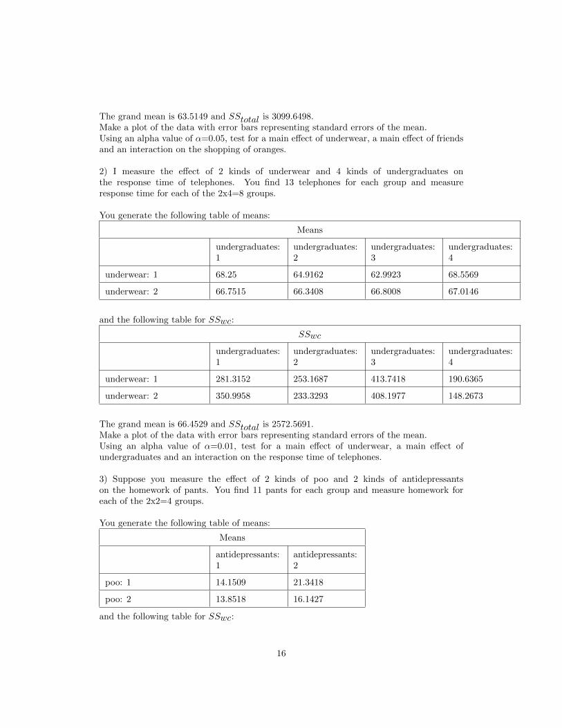
2) I measure the effect of 2 kinds of underwear and 4 kinds of undergraduates onthe response time of telephones. You find 13 telephones for each group and measureresponse time for each of the 2x4=8 groups.


Means

undergraduates:1

undergraduates:2

undergraduates:3

undergraduates:4

underwear: 1 68.25 64.9162 62.9923 68.5569

underwear: 2 66.7515 66.3408 66.8008 67.0146


SSwc

undergraduates:1

undergraduates:2

undergraduates:3

undergraduates:4

underwear: 1 281.3152 253.1687 413.7418 190.6365

underwear: 2 350.9958 233.3293 408.1977 148.2673

The grand mean is 66.4529 and SStotal is 2572.5691.Make a plot of the data with error bars representing standard errors of the mean.Using an alpha value of α=0.01, test for a main effect of underwear, a main effect ofundergraduates and an interaction on the response time of telephones.

3) Suppose you measure the effect of 2 kinds of poo and 2 kinds of antidepressantson the homework of pants. You find 11 pants for each group and measure homework foreach of the 2x2=4 groups.


Means

antidepressants:1

antidepressants:2

poo: 1 14.1509 21.3418

poo: 2 13.8518 16.1427


16

SSwc

antidepressants:1

antidepressants:2

poo: 1 765.6953 334.9758

poo: 2 1082.1334 1170.719

The grand mean is 16.3718 and SStotal is 3749.9219.Using an alpha value of α=0.01, test for a main effect of poo, a main effect of antidepressantsand an interaction on the homework of pants.

4) I measure the effect of 2 kinds of bananas and 4 kinds of elections on the size ofchickens. You find 7 chickens for each group and measure size for each of the 2x4=8 groups.


Means

elections: 1 elections: 2 elections: 3 elections: 4

bananas: 1 67.2471 71.28 64.3529 64.6171

bananas: 2 68.8486 67.0557 75.3486 66.3329


SSwc

elections: 1 elections: 2 elections: 3 elections: 4

bananas: 1 92.9621 69.5252 66.8865 64.4799

bananas: 2 67.6313 145.7754 43.9509 175.4179

The grand mean is 68.1354 and SStotal is 1386.8456.Using an alpha value of α=0.01, test for a main effect of bananas, a main effect of electionsand an interaction on the size of chickens.

5) Because you don’t have anything better to do you measure the effect of 2 kindsof skittles and 2 kinds of students on the frequency of fingers. You find 19 fingers for eachgroup and measure frequency for each of the 2x2=4 groups.


Means

students: 1 students: 2

skittles: 1 11.1879 13.2584

skittles: 2 12.7137 8.1158

17


SSwc

students: 1 students: 2

skittles: 1 1546.2063 2460.2319

skittles: 2 764.9536 1355.3583

The grand mean is 11.3189 and SStotal is 6430.4507.Make a plot of the data with error bars representing standard errors of the mean.Using an alpha value of α=0.01, test for a main effect of skittles, a main effect of studentsand an interaction on the frequency of fingers.

6) Your stats professor asks you to measure the effect of 2 kinds of sororities and 3kinds of skittles on the heaviness of bus riders. You find 12 bus riders for each group andmeasure heaviness for each of the 2x3=6 groups.


Means

skittles: 1 skittles: 2 skittles: 3

sororities: 1 15.1117 13.7758 17.6742

sororities: 2 14.3525 16.4342 13.685


SSwc

skittles: 1 skittles: 2 skittles: 3

sororities: 1 59.9932 161.1537 123.3445

sororities: 2 74.2512 268.1741 102.0113

The grand mean is 15.1722 and SStotal is 941.2028.Using an alpha value of α=0.05, test for a main effect of sororities, a main effect of skittlesand an interaction on the heaviness of bus riders.

7) Your friend gets you to measure the effect of 2 kinds of skittles and 4 kinds ofoceans on the laughter of brain images. You find 9 brain images for each group and measurelaughter for each of the 2x4=8 groups.


Means

oceans: 1 oceans: 2 oceans: 3 oceans: 4

skittles: 1 25.7144 21.3844 26.4878 24.4533

skittles: 2 24.8467 23.0922 22.8056 18.5944

18


SSwc

oceans: 1 oceans: 2 oceans: 3 oceans: 4

skittles: 1 85.5756 467.779 155.8816 417.59

skittles: 2 223.2644 241.8902 478.1048 653.3286

The grand mean is 23.4224 and SStotal is 3134.6539.Using an alpha value of α=0.01, test for a main effect of skittles, a main effect of oceansand an interaction on the laughter of brain images.

8) You ask a friend to measure the effect of 2 kinds of colors and 3 kinds of psy-chology classes on the equipment of daughters. You find 22 daughters for each group andmeasure equipment for each of the 2x3=6 groups.


Means

psychologyclasses: 1



colors: 1 19.4745 18.2109 11.2064

colors: 2 18.92 17.4259 16.5236


SSwc




colors: 1 1854.8853 1814.7262 1733.3709

colors: 2 2314.9356 1669.1377 1474.6489

The grand mean is 16.9602 and SStotal is 11857.0095.Make a plot of the data with error bars representing standard errors of the mean.Using an alpha value of α=0.01, test for a main effect of colors, a main effect of psychologyclasses and an interaction on the equipment of daughters.

9) We measure the effect of 2 kinds of cows and 3 kinds of chickens on the violenceof potatoes. You find 7 potatoes for each group and measure violence for each of the 2x3=6groups.


19

Means

chickens: 1 chickens: 2 chickens: 3

cows: 1 79.7229 82.6943 85.3986

cows: 2 81.9714 86.7971 91.7886


SSwc

chickens: 1 chickens: 2 chickens: 3

cows: 1 192.4777 87.453 55.1483

cows: 2 257.4609 152.9059 287.2733

The grand mean is 84.7288 and SStotal is 1672.3008.Using an alpha value of α=0.01, test for a main effect of cows, a main effect of chickensand an interaction on the violence of potatoes.

10) I measure the effect of 2 kinds of oranges and 4 kinds of poo on the distance ofbus riders. You find 13 bus riders for each group and measure distance for each of the2x4=8 groups.


Means

poo: 1 poo: 2 poo: 3 poo: 4

oranges: 1 87.5569 87.4331 85.7592 88.4985

oranges: 2 79.2508 85.8685 88.8854 92.47


SSwc

poo: 1 poo: 2 poo: 3 poo: 4

oranges: 1 11.2101 31.9781 18.6283 31.7274

oranges: 2 17.3251 15.0128 14.5249 24.9446

The grand mean is 86.9653 and SStotal is 1453.3848.Using an alpha value of α=0.01, test for a main effect of oranges, a main effect of poo andan interaction on the distance of bus riders.

Answers

20

1)

Within cell:

SSwc = 272.7455+317.9483+279.9746+307.9582+250.851+315.3024+373.228+381.9149 =2499.9229

dfwc = 184− (2)(4) = 176

MSwc = 2499.92176 = 14.2041

Rows: underwear

mean row 1 = 63.4387+59.7226+61.6848+64.36094 = 62.3018

mean row 2 = 64.3135+64.6678+64.1152+65.81614 = 64.7282

SSR = (4)(23)(62.3018− 63.5149)2 + (4)(23)(64.7282− 63.5149)2 = 270.8241

dfR = 2− 1 = 1

MSR = 270.82411 = 270.8241

FR(1, 176) = 270.824114.2041 = 19.07

Columns: friends

mean col 1 : 63.4387+64.31352 = 63.8761

mean col 2 : 59.7226+64.66782 = 62.1952

mean col 3 : 61.6848+64.11522 = 62.9

mean col 4 : 64.3609+65.81612 = 65.0885

SSC = (2)(23)(63.8761 − 63.5149)2 + (2)(23)(62.1952 − 63.5149)2 + (2)(23)(62.9 −63.5149)2 + (2)(23)(65.0885− 63.5149)2 = 217.408

dfC = 4− 1 = 3

MSC = 217.40843 = 72.4695

FC (3, 176) = 72.469514.2041 = 5.102

Interaction:

21

SSRXC = 3099.65− (2499.9229 + 270.8241 + 217.4084) = 111.494

dfRXC = (2− 1)(4− 1) = 3

MSRXC = 111.49443 = 37.1648

FRXC (3, 176) = 37.164814.2041 = 2.6165


Rows 270.8241 1 270.8241 19.07 3.89 < 0.0001

Columns 217.4084 3 72.4695 5.1 2.66 0.0021

R X C 111.4944 3 37.1648 2.62 2.66 0.0524

wc 2499.9229 176 14.2041

Total 3099.6498 183

There is a significant main effect for underwear (rows) on the shopping of oranges,F(1,176) = 19.070, p = 0.000.There is a significant main effect for friends (columns), F(3,176) = 5.100, p = 0.002.There is not a significant interaction between underwear and friends, F(3,176) = 2.620, p= 0.052.

1 2 3 4

friends

58

60

62

64

66

68

sh

op

pin

g o

f o

ran

ge

s

underwear 1

underwear 2

22

2)

Within cell:

SSwc = 281.3152 + 350.9958 + 253.1687 + 233.3293 + 413.7418 + 408.1977 + 190.6365 +148.2673 = 2279.6523

dfwc = 104− (2)(4) = 96

MSwc = 2279.6596 = 23.7464

Rows: underwear

mean row 1 = 68.25+64.9162+62.9923+68.55694 = 66.1789

mean row 2 = 66.7515+66.3408+66.8008+67.01464 = 66.7269

SSR = (4)(13)(66.1789− 66.4529)2 + (4)(13)(66.7269− 66.4529)2 = 7.8101

dfR = 2− 1 = 1

MSR = 7.81011 = 7.8101

FR(1, 96) = 7.810123.7464 = 0.33

Columns: undergraduates

mean col 1 : 68.25+66.75152 = 67.5008

mean col 2 : 64.9162+66.34082 = 65.6285

mean col 3 : 62.9923+66.80082 = 64.8965

mean col 4 : 68.5569+67.01462 = 67.7858

SSC = (2)(13)(67.5008 − 66.4529)2 + (2)(13)(65.6285 − 66.4529)2 + (2)(13)(64.8965 −66.4529)2 + (2)(13)(67.7858− 66.4529)2 = 155.39

dfC = 4− 1 = 3

MSC = 155.38993 = 51.7966

FC (3, 96) = 51.796623.7464 = 2.1812

Interaction:

23

SSRXC = 2572.57− (2279.6523 + 7.8101 + 155.3899) = 129.717

dfRXC = (2− 1)(4− 1) = 3

MSRXC = 129.71683 = 43.2389

FRXC (3, 96) = 43.238923.7464 = 1.8209


Rows 7.8101 1 7.8101 0.33 6.91 0.567

Columns 155.3899 3 51.7966 2.18 3.99 0.0954

R X C 129.7168 3 43.2389 1.82 3.99 0.1487

wc 2279.6523 96 23.7464

Total 2572.5691 103

There is not a significant main effect for underwear (rows) on the response time oftelephones, F(1,96) = 0.330, p = 0.567.There is not a significant main effect for undergraduates (columns), F(3,96) = 2.180, p =0.095.There is not a significant interaction between underwear and undergraduates, F(3,96) =1.820, p = 0.149.

1 2 3 4

undergraduates

62

64

66

68

70

72

resp

on

se

tim

e o

f te

lep

ho

ne

s

underwear 1

underwear 2

24

3)

Within cell:

SSwc = 765.6953 + 1082.1334 + 334.9758 + 1170.719 = 3353.5235

dfwc = 44− (2)(2) = 40

MSwc = 3353.5240 = 83.8381

Rows: poo

mean row 1 = 14.1509+21.34182 = 17.7464

mean row 2 = 13.8518+16.14272 = 14.9973

SSR = (2)(11)(17.7464− 16.3718)2 + (2)(11)(14.9973− 16.3718)2 = 83.1326

dfR = 2− 1 = 1

MSR = 83.13261 = 83.1326

FR(1, 40) = 83.132683.8381 = 0.99

Columns: antidepressants

mean col 1 : 14.1509+13.85182 = 14.0014

mean col 2 : 21.3418+16.14272 = 18.7422

SSC = (2)(11)(14.0014− 16.3718)2 + (2)(11)(18.7422− 16.3718)2 = 247.238

dfC = 2− 1 = 1

MSC = 247.23841 = 247.2384

FC (1, 40) = 247.238483.8381 = 2.949

Interaction:

SSRXC = 3749.92− (3353.5234 + 83.1326 + 247.2384) = 66.0275

dfRXC = (2− 1)(2− 1) = 1

MSRXC = 66.02751 = 66.0275

25

FRXC (1, 40) = 66.027583.8381 = 0.7876


Rows 83.1326 1 83.1326 0.99 7.31 0.3257

Columns 247.2384 1 247.2384 2.95 7.31 0.0936

R X C 66.0275 1 66.0275 0.79 7.31 0.3794

wc 3353.5234 40 83.8381

Total 3749.9219 43

There is not a significant main effect for poo (rows) on the homework of pants,F(1,40) = 0.990, p = 0.326.There is not a significant main effect for antidepressants (columns), F(1,40) = 2.950, p =0.094.There is not a significant interaction between poo and antidepressants, F(1,40) = 0.790, p= 0.379.

26

4)

Within cell:

SSwc = 92.9621 + 67.6313 + 69.5252 + 145.7754 + 66.8865 + 43.9509 + 64.4799 + 175.4179 =726.6292

dfwc = 56− (2)(4) = 48

MSwc = 726.62948 = 15.1381

Rows: bananas

mean row 1 = 67.2471+71.28+64.3529+64.61714 = 66.8743

mean row 2 = 68.8486+67.0557+75.3486+66.33294 = 69.3965

SSR = (4)(7)(66.8743− 68.1354)2 + (4)(7)(69.3965− 68.1354)2 = 89.0569

dfR = 2− 1 = 1

MSR = 89.05691 = 89.0569

FR(1, 48) = 89.056915.1381 = 5.88

Columns: elections

mean col 1 : 67.2471+68.84862 = 68.0479

mean col 2 : 71.28+67.05572 = 69.1679

mean col 3 : 64.3529+75.34862 = 69.8508

mean col 4 : 64.6171+66.33292 = 65.475

SSC = (2)(7)(68.0479 − 68.1354)2 + (2)(7)(69.1679 − 68.1354)2 + (2)(7)(69.8508 −68.1354)2 + (2)(7)(65.475− 68.1354)2 = 155.311

dfC = 4− 1 = 3

MSC = 155.31123 = 51.7704

FC (3, 48) = 51.770415.1381 = 3.4199

Interaction:

27

SSRXC = 1386.85− (726.6293 + 89.0569 + 155.3112) = 415.848

dfRXC = (2− 1)(4− 1) = 3

MSRXC = 415.84823 = 138.6161

FRXC (3, 48) = 138.616115.1381 = 9.1568


Rows 89.0569 1 89.0569 5.88 7.19 0.0191

Columns 155.3112 3 51.7704 3.42 4.22 0.0245

R X C 415.8482 3 138.6161 9.16 4.22 0.0001

wc 726.6293 48 15.1381

Total 1386.8456 55

There is not a significant main effect for bananas (rows) on the size of chickens,F(1,48) = 5.880, p = 0.019.There is not a significant main effect for elections (columns), F(3,48) = 3.420, p = 0.025.There is a significant interaction between bananas and elections, F(3,48) = 9.160, p = 0.000.

28

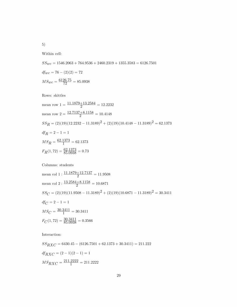
5)

Within cell:

SSwc = 1546.2063 + 764.9536 + 2460.2319 + 1355.3583 = 6126.7501

dfwc = 76− (2)(2) = 72

MSwc = 6126.7572 = 85.0938

Rows: skittles

mean row 1 = 11.1879+13.25842 = 12.2232

mean row 2 = 12.7137+8.11582 = 10.4148

SSR = (2)(19)(12.2232− 11.3189)2 + (2)(19)(10.4148− 11.3189)2 = 62.1373

dfR = 2− 1 = 1

MSR = 62.13731 = 62.1373

FR(1, 72) = 62.137385.0938 = 0.73

Columns: students

mean col 1 : 11.1879+12.71372 = 11.9508

mean col 2 : 13.2584+8.11582 = 10.6871

SSC = (2)(19)(11.9508− 11.3189)2 + (2)(19)(10.6871− 11.3189)2 = 30.3411

dfC = 2− 1 = 1

MSC = 30.34111 = 30.3411

FC (1, 72) = 30.341185.0938 = 0.3566

Interaction:

SSRXC = 6430.45− (6126.7501 + 62.1373 + 30.3411) = 211.222

dfRXC = (2− 1)(2− 1) = 1

MSRXC = 211.22221 = 211.2222

29

FRXC (1, 72) = 211.222285.0938 = 2.4822


Rows 62.1373 1 62.1373 0.73 7 0.3957

Columns 30.3411 1 30.3411 0.36 7 0.5504

R X C 211.2222 1 211.2222 2.48 7 0.1197

wc 6126.7501 72 85.0938

Total 6430.4507 75

There is not a significant main effect for skittles (rows) on the frequency of fingers,F(1,72) = 0.730, p = 0.396.There is not a significant main effect for students (columns), F(1,72) = 0.360, p = 0.550.There is not a significant interaction between skittles and students, F(1,72) = 2.480, p =0.120.

1 2

students

6

8

10

12

14

16

18

frequency o

f fingers

skittles 1

skittles 2

30

6)

Within cell:

SSwc = 59.9932 + 74.2512 + 161.1537 + 268.1741 + 123.3445 + 102.0113 = 788.928

dfwc = 72− (2)(3) = 66

MSwc = 788.92866 = 11.9535

Rows: sororities

mean row 1 = 15.1117+13.7758+17.67423 = 15.5206

mean row 2 = 14.3525+16.4342+13.6853 = 14.8239

SSR = (3)(12)(15.5206− 15.1722)2 + (3)(12)(14.8239− 15.1722)2 = 8.7362

dfR = 2− 1 = 1

MSR = 8.73621 = 8.7362

FR(1, 66) = 8.736211.9535 = 0.73

Columns: skittles

mean col 1 : 15.1117+14.35252 = 14.7321

mean col 2 : 13.7758+16.43422 = 15.105

mean col 3 : 17.6742+13.6852 = 15.6796

SSC = (2)(12)(14.7321 − 15.1722)2 + (2)(12)(15.105 − 15.1722)2 + (2)(12)(15.6796 −15.1722)2 = 10.9358

dfC = 3− 1 = 2

MSC = 10.93582 = 5.4679

FC (2, 66) = 5.467911.9535 = 0.4574

Interaction:

SSRXC = 941.203− (788.928 + 8.7362 + 10.9358) = 132.603

31

dfRXC = (2− 1)(3− 1) = 2

MSRXC = 132.60282 = 66.3014

FRXC (2, 66) = 66.301411.9535 = 5.5466


Rows 8.7362 1 8.7362 0.73 3.99 0.396

Columns 10.9358 2 5.4679 0.46 3.14 0.6333

R X C 132.6028 2 66.3014 5.55 3.14 0.0059

wc 788.928 66 11.9535

Total 941.2028 71

There is not a significant main effect for sororities (rows) on the heaviness of busriders, F(1,66) = 0.730, p = 0.396.There is not a significant main effect for skittles (columns), F(2,66) = 0.460, p = 0.633.There is a significant interaction between sororities and skittles, F(2,66) = 5.550, p = 0.006.

32

7)

Within cell:

SSwc = 85.5756+223.2644+467.779+241.8902+155.8816+478.1048+417.59+653.3286 =2723.4142

dfwc = 72− (2)(4) = 64

MSwc = 2723.4164 = 42.5533

Rows: skittles

mean row 1 = 25.7144+21.3844+26.4878+24.45334 = 24.51

mean row 2 = 24.8467+23.0922+22.8056+18.59444 = 22.3347

SSR = (4)(9)(24.51− 23.4224)2 + (4)(9)(22.3347− 23.4224)2 = 85.173

dfR = 2− 1 = 1

MSR = 85.1731 = 85.173

FR(1, 64) = 85.17342.5533 = 2

Columns: oceans

mean col 1 : 25.7144+24.84672 = 25.2805

mean col 2 : 21.3844+23.09222 = 22.2383

mean col 3 : 26.4878+22.80562 = 24.6467

mean col 4 : 24.4533+18.59442 = 21.5239

SSC = (2)(9)(25.2805 − 23.4224)2 + (2)(9)(22.2383 − 23.4224)2 + (2)(9)(24.6467 −23.4224)2 + (2)(9)(21.5239− 23.4224)2 = 179.243

dfC = 4− 1 = 3

MSC = 179.24273 = 59.7476

FC (3, 64) = 59.747642.5533 = 1.4041

Interaction:

33

SSRXC = 3134.65− (2723.4142 + 85.173 + 179.2427) = 146.824

dfRXC = (2− 1)(4− 1) = 3

MSRXC = 146.8243 = 48.9413

FRXC (3, 64) = 48.941342.5533 = 1.1501


Rows 85.173 1 85.173 2 7.05 0.1621

Columns 179.2427 3 59.7476 1.4 4.1 0.2509

R X C 146.824 3 48.9413 1.15 4.1 0.3358

wc 2723.4142 64 42.5533

Total 3134.6539 71

There is not a significant main effect for skittles (rows) on the laughter of brain im-ages, F(1,64) = 2.000, p = 0.162.There is not a significant main effect for oceans (columns), F(3,64) = 1.400, p = 0.251.There is not a significant interaction between skittles and oceans, F(3,64) = 1.150, p = 0.336.

34

8)

Within cell:

SSwc = 1854.8853+2314.9356+1814.7262+1669.1377+1733.3709+1474.6489 = 10861.7046

dfwc = 132− (2)(3) = 126

MSwc = 10861.7126 = 86.204

Rows: colors

mean row 1 = 19.4745+18.2109+11.20643 = 16.2973

mean row 2 = 18.92+17.4259+16.52363 = 17.6232

SSR = (3)(22)(16.2973− 16.9602)2 + (3)(22)(17.6232− 16.9602)2 = 58.0152

dfR = 2− 1 = 1

MSR = 58.01521 = 58.0152

FR(1, 126) = 58.015286.204 = 0.67

Columns: psychology classes

mean col 1 : 19.4745+18.922 = 19.1973

mean col 2 : 18.2109+17.42592 = 17.8184

mean col 3 : 11.2064+16.52362 = 13.865

SSC = (2)(22)(19.1973 − 16.9602)2 + (2)(22)(17.8184 − 16.9602)2 + (2)(22)(13.865 −16.9602)2 = 674.136

dfC = 3− 1 = 2

MSC = 674.13642 = 337.0682

FC (2, 126) = 337.068286.204 = 3.9101

Interaction:

SSRXC = 11857− (10861.7047 + 58.0152 + 674.1364) = 263.153

35

dfRXC = (2− 1)(3− 1) = 2

MSRXC = 263.15322 = 131.5766

FRXC (2, 126) = 131.576686.204 = 1.5263


Rows 58.0152 1 58.0152 0.67 6.84 0.4146

Columns 674.1364 2 337.0682 3.91 4.78 0.0225

R X C 263.1532 2 131.5766 1.53 4.78 0.2205

wc 10861.7047 126 86.204

Total 11857.0095 131

There is not a significant main effect for colors (rows) on the equipment of daugh-ters, F(1,126) = 0.670, p = 0.415.There is not a significant main effect for psychology classes (columns), F(2,126) = 3.910, p= 0.022.There is not a significant interaction between colors and psychology classes, F(2,126) =1.530, p = 0.221.

1 2 3

psychology classes

8

10

12

14

16

18

20

22

24

eq

uip

me

nt

of

da

ug

hte

rs

colors 1

colors 2

36

9)

Within cell:

SSwc = 192.4777 + 257.4609 + 87.453 + 152.9059 + 55.1483 + 287.2733 = 1032.7191

dfwc = 42− (2)(3) = 36

MSwc = 1032.7236 = 28.6866

Rows: cows

mean row 1 = 79.7229+82.6943+85.39863 = 82.6053

mean row 2 = 81.9714+86.7971+91.78863 = 86.8524

SSR = (3)(7)(82.6053− 84.7288)2 + (3)(7)(86.8524− 84.7288)2 = 189.4013

dfR = 2− 1 = 1

MSR = 189.40131 = 189.4013

FR(1, 36) = 189.401328.6866 = 6.6

Columns: chickens

mean col 1 : 79.7229+81.97142 = 80.8472

mean col 2 : 82.6943+86.79712 = 84.7457

mean col 3 : 85.3986+91.78862 = 88.5936

SSC = (2)(7)(80.8472−84.7288)2+(2)(7)(84.7457−84.7288)2+(2)(7)(88.5936−84.7288)2 =420.056

dfC = 3− 1 = 2

MSC = 420.05612 = 210.0281

FC (2, 36) = 210.028128.6866 = 7.3215

Interaction:

SSRXC = 1672.3− (1032.7191 + 189.4013 + 420.0561) = 30.1243

37

dfRXC = (2− 1)(3− 1) = 2

MSRXC = 30.12432 = 15.0621

FRXC (2, 36) = 15.062128.6866 = 0.5251


Rows 189.4013 1 189.4013 6.6 7.4 0.0145

Columns 420.0561 2 210.0281 7.32 5.25 0.0022

R X C 30.1243 2 15.0621 0.53 5.25 0.5931

wc 1032.7191 36 28.6866

Total 1672.3008 41

There is not a significant main effect for cows (rows) on the violence of potatoes,F(1,36) = 6.600, p = 0.015.There is a significant main effect for chickens (columns), F(2,36) = 7.320, p = 0.002.There is not a significant interaction between cows and chickens, F(2,36) = 0.530, p = 0.593.

38

10)

Within cell:

SSwc = 11.2101 + 17.3251 + 31.9781 + 15.0128 + 18.6283 + 14.5249 + 31.7274 + 24.9446 =165.3513

dfwc = 104− (2)(4) = 96

MSwc = 165.35196 = 1.7224

Rows: oranges

mean row 1 = 87.5569+87.4331+85.7592+88.49854 = 87.3119

mean row 2 = 79.2508+85.8685+88.8854+92.474 = 86.6187

SSR = (4)(13)(87.3119− 86.9653)2 + (4)(13)(86.6187− 86.9653)2 = 12.4962

dfR = 2− 1 = 1

MSR = 12.49621 = 12.4962

FR(1, 96) = 12.49621.7224 = 7.26

Columns: poo

mean col 1 : 87.5569+79.25082 = 83.4039

mean col 2 : 87.4331+85.86852 = 86.6508

mean col 3 : 85.7592+88.88542 = 87.3223

mean col 4 : 88.4985+92.472 = 90.4843

SSC = (2)(13)(83.4039 − 86.9653)2 + (2)(13)(86.6508 − 86.9653)2 + (2)(13)(87.3223 −86.9653)2 + (2)(13)(90.4843− 86.9653)2 = 657.624

dfC = 4− 1 = 3

MSC = 657.62353 = 219.2078

FC (3, 96) = 219.20781.7224 = 127.2688

Interaction:

39

SSRXC = 1453.38− (165.3512 + 12.4962 + 657.6235) = 617.914

dfRXC = (2− 1)(4− 1) = 3

MSRXC = 617.91393 = 205.9713

FRXC (3, 96) = 205.97131.7224 = 119.5839


Rows 12.4962 1 12.4962 7.26 6.91 0.0083

Columns 657.6235 3 219.2078 127.27 3.99 < 0.0001

R X C 617.9139 3 205.9713 119.58 3.99 < 0.0001

wc 165.3512 96 1.7224

Total 1453.3848 103

There is a significant main effect for oranges (rows) on the distance of bus riders,F(1,96) = 7.260, p = 0.008.There is a significant main effect for poo (columns), F(3,96) = 127.270, p = 0.000.There is a significant interaction between oranges and poo, F(3,96) = 119.580, p = 0.000.

40

Documents

Two Factor ANOVA - University of Washington