Tutorial Pattern Recognition in Pharmacokinetic Data Analysis

Tutorial

Pattern Recognition in Pharmacokinetic Data Analysis

Johan Gabrielsson,1,4 Bernd Meibohm,2 and Daniel Weiner3

Received 6 May 2015; accepted 13 August 2015; published online 3 September 2015

Abstract. Pattern recognition is a key element in pharmacokinetic data analyses when first selecting amodel to be regressed to data. We call this process going from data to insight and it is an important aspectof exploratory data analysis (EDA). But there are very few formal ways or strategies that scientiststypically use when the experiment has been done and data collected. This report deals with identifyingthe properties of a kinetic model by dissecting the pattern that concentration-time data reveal. Patternrecognition is a pivotal activity when modeling kinetic data, because a rigorous strategy is essential fordissecting the determinants behind concentration-time courses. First, we extend a commonly usedrelationship for calculation of the number of potential model parameters by simultaneously utilizing allconcentration-time courses. Then, a set of points to consider are proposed that specifically addressesexploratory data analyses, number of phases in the concentration-time course, baseline behavior, timedelays, peak shifts with increasing doses, flip-flop phenomena, saturation, and other potentialnonlinearities that an experienced eye catches in the data. Finally, we set up a series of equationsrelated to the patterns. In other words, we look at what causes the shapes that make up theconcentration-time course and propose a strategy to construct a model. By practicing pattern recognition,one can significantly improve the quality and timeliness of data analysis and model building. Aconsequence of this is a better understanding of the complete concentration-time profile.

KEY WORDS: absorption; area under the curve; bi-exponential; half-life; induction; intravenous andextravascular dosing; lag time; mono-exponential; multi-compartment; nonlinear elimination; plasmaconcentration-time courses; target-mediated drug disposition; transporters.

INTRODUCTION

Pattern recognition is a key element in pharmacokineticdata analyses when first selecting a model to be regressed todata. We call this process going from data to insight. Butthere are no formal best practices that scientists typically use.This report deals with identifying the properties of a kineticmodel by dissecting the pattern that concentration-time datareveal graphically. Pattern recognition is a pivotal activitywhen modeling pharmacokinetic data, because a rigorousstrategy is essential for dissecting the determinants behindconcentration-time courses. In the pharmacology field, patternrecognition has also been proposed for interpreting results ofdrug-drug interactions (1).

The format of the presentation order of the data sets areshown in Fig. 1. The route of administration is the top level.Under that, we split into intravenous (iv, disposition kinetics)dosing and extravascular (ev, po, absorption confounded

kinetics) of single- (mono-exponential decline) and multiple-compartment (multi-exponential decline) systems. The nextlevel discriminates between linear- and nonlinear systems.This order is, what we assume, that one immediately can seefrom a semi-logarithmic graph of concentration-time data. Aspecial case of extravascular administration where one has todiscriminate between first- and zero-order input is also given.

The 16 data schemes we are going to discuss are shownschematically in Fig. 2. These are representative of differentpatterns typically seen in in vivo pharmacokinetic practice.For each case study, we will provide the underlying modelincluding the differential equations that describe the system,the parameters and constants, and the number of functions(datasets) involved in the regression analysis.

The following strategy was adopted:

& In case studies 1 and 2, we explore intravenous ivbolus dosing of a one (two subjects with differentclearances and similar volumes) and two compart-ments (two populations, clamped and normal withdifferent clearances and effective half-lives).

& Then, we move on to extravascular dosing in casestudies 3 and 4, where a one-compartment first-orderinput/output systems with and without lag time, andiv and extravascular dosing for a two-compartmentsystem, respectively.

& In case study 5, we revisit extravascular (po) dosingalthough we observe rapid absorption, lag time, and

1Department of Biomedical Sciences and Veterinary Public Health,SLU, Division of Pharmacology and Toxicology, Box 7028, SE-750 07,Uppsala, Sweden.

2 College of Pharmacy, University of Tennessee Health ScienceCenter, 881 Madison Avenue, Rm. 444, Memphis, Tennessee38163, USA.

3 709 Cambridge Hall Loop, Apex, North Carolina 27539, USA.4 To whom correspondence should be addressed. (e-mail:[email protected])

The AAPS Journal, Vol. 18, No. 1, January 2016 (# 2015)DOI: 10.1208/s12248-015-9817-6

47 1550-7416/1 /0100-0047/0 # 2015 American Association of Pharmaceutical Scientists6

multi-exponential decline post-peak. This datasetdoes not contain iv data.

& Case study 6 returns to iv bolus dosing and mono-exponential decline in plasma but is extended alsowith urinary data so renal clearance or fractionexcreted into the urine can be estimated simulta-neously with total clearance.

& Case studies 7 and 8 are also iv dosing coveringmono- and bi-exponential decline for two systemsthat exhibit saturable (nonlinear) clearance terms.

& Two nonlinear systems are also presented after oraldosing in case studies 9 and 10. The former capturesnonlinear elimination and the latter saturable absorp-tion via transporters.

& We extend the analyses by looking at iv (case study 11)and subcutaneous (sc) (case study 12) of two systemswith endogenous levels of the test compound. Thisextends the model with one additional parameter, theturnover rate.

& The last four case studies (case studies 13–16) areextensions looking at target-mediated drug disposi-tion (case study 13), time-dependent induction ofclearance (case study 14), simultaneous fitting ofnonlinear multi-compartment kinetics of parent com-pound and metabolite after three different iv doses,and then finally fitting a first- and zero-order absorp-tion model to an oral dosing dataset.

We encourage the analyst to regress several sources ofdata simultaneously if possible. In case study 4, a full two-compartment system is revealed in iv data but not in ev data.This dataset is contrasted with case study 5 where only evdata are available. However, the latter still displays a multi-compartment behavior due to the rapid absorption. Both casestudies 4 and 5 are commonly encountered situation which isthe reason why they may be of interest to the reader. Several

Fig. 1. Decision-tree structure of the analyzed case studies.Numeralrefer to the case studies.

Fig. 2. Schematic illustration of the 16 data patterns discussed in this report. 1 Two individuals with mono-exponential disposition. 2 Bi-exponentialdecline after iv bolus dosing in two groups of animals. 3 Lag time or no lag time in the absorption process with absorption rate-limited elimination. 4Simultaneous analysis of bi-exponential decline after iv dosing and mono-exponential decline when dosing orally. 5Multi-exponential behavior afteroral dosing. 6 Plasma and cumulative urine data. 7 Single-compartment disposition coupled to nonlinear elimination. 8 Multi-compartmentdisposition coupled to nonlinear elimination. 9 Nonlinear elimination after oral dosing. 10 Saturable absorption by transporters. 11 Bi-exponentialdecline after bolus dosing with a baseline value. 12 Extravascular administration of an endogenous compound with a baseline value. 13 Target-mediated drug disposition. 14Multiple dosing coupled to a period of hetero-induction shown by the gray horizontal bar. 15 Nonlinear formation ofmetabolite (dashed lines) after iv dosing of parent compound (solid lines). 16 First- and zero-order absorption patterns. All plots are semi-logarithmicexcept 12, 14, and 16 where data are displayed on a linear scale due to a limited concentration range.

48 Gabrielsson et al.

sources of data are further elaborated on in case studies 6, 7,9, 10, 13, and 15. Further comparisons across two or morecase studies are done at the end of relevant cases.

A schematic diagram of each model proposed for thedata schemes in Fig. 2 is shown in Fig. 3.

A set of points to consider are proposed that specificallyaddresses exploratory data analyses, number of phases in theconcentration-time course, convex or concave curvature,baseline behavior, time delay, lag time, peak shifts withincreasing doses, flip-flop phenomena, saturation, and otherpotential nonlinearities that the eye catches in the data. Welook at what causes the shapes that make up theconcentration-time course. By practicing pattern recogni-tion, one can significantly improve the quality of dataanalysis and model building. A consequence of this is abetter understanding of the complete concentration-timeprofile. We have therefore collected a set of patternsextracted from literature data and then modified them sothe typical features emerge more clearly (2). We alsopropose alternative solutions to the patterns.

The number of parameters NP which can be calculatedfor a given model is dependent on the number of exponen-tials EX post-peak visible in the plasma concentration-timeprofile, the number of elimination or excretory pathways PE

suitably measured, the number of tissue spaces or bindingproteins TS analyzed, and the number of visible nonlinearfeatures NL in the data (Eq. 1, top). This expression wasproposed by Jusko and meant to be a guidance function(a set of numerical points to consider) when dissectingpharmacokinetic profiles (3). We have personally benefittedfrom this simple but elegant tool as a starting point in our ownanalyses. An extension (Eq. 1, bottom) of the original model ispresented here which also includes information about absorp-tion ABS, initial time delays TLG, baseline BL, and potentialmetabolite(s) MTB

Original model NP ¼ 2⋅EXþ PEþ 2⋅TSþNL

Extended model NP ¼ 2⋅EXþ PEþ 2⋅TSþNLþABSþ TLGþ BLþ 2⋅MTB

8<:

ð1Þ

Equation 1 is applicable if sufficient and accurate dataare obtained and can be extended. For example, if we havedata after an intravenous bolus dose that decline in a bi-exponential fashion (i.e., with an α and a β phase), then it ispossible to estimate 2 EX=4 parameters (i.e., A, α, B, and β).If we also have measured drug excretion in urine, we could

Fig. 3. Schematic diagram of each model used for the analysis of concentration-time data shown in Figs. 2, 4, 5, 6, and 7. All parameters andvariables are explained in their respective case study sections. Numerals above the figures refer to the respective case study.

49Pattern Recognition in Pharmacokinetic Data Analysis

estimate renal clearance or fraction of dose excreted via theurine PE. If, in addition to the bi-exponential decline inplasma 2 EX, we have a nonlinear feature NL and urinarydata PE, we might be able to estimate six parameters.

Equation 1 was suggested as a practical tool for theidentification of a possible number of estimable parametersbased on observable patterns of the drug moiety as such inplasma. We will also see how applicable the extended Eq. 1 isto the 16 datasets provided. Equation 1 should be used withcareful attention to the quality of data, the design of theexperiment, and when the number of data sources beyondparent compound in plasma and urine are available. Simul-taneous fitting of all available sources of data is alwaysrecommended.

This report focuses on the practical identifiability ofpharmacokinetic parameters based on visual inspection ofexperimental data. First, we extend a commonly usedrelationship for calculation of the number of potential modelparameters by simultaneously utilizing all concentration-timecourses. Then, a set of points to consider is proposed thatspecifically addresses exploratory data analyses, number ofphases in the concentration-time course, baseline behavior,time delays, peak shifts with increasing doses, flip-flopphenomena, saturation, and other potential nonlinearitiesthat an experienced eye catches in the data. Finally, we setup a series of equations related to the patterns and themes.Theoretical a priori identifiability of pharmacokinetic parametershas been discussed by others (4) and will not be addressed here.

Case study 1. A mono-exponential decline is observed inplasma after an intravenous bolus dose to two subjects (Fig. 4,case study 1 (2)). Both subjects received the same amount oftest compound. The goal is to identify typical signs ofpharmacokinetic similarities and differences between thesetwo concentration-time courses. In other words, what are themost obvious characteristics that one may pick out by visualinspection of data?

The mono-exponential decline shown in Fig. 4 (casestudy 1) on logarithmic concentration scale can be describedmathematically as a first-order differential equation.

dCdt

¼ −K⋅C ¼ −ClV

⋅C ð2Þ

dC/dt is the rate of change of the plasma concentration,C is the plasma concentration, and K is the first-order rateconstant associated with the elimination process. A newparameter, clearance Cl, is then introduced. Clearance isdefined as the volume of blood or plasma that is totallycleared of its content of drug per unit time (mL min−1 orL min−1). The other parameter of primary interest is thevolume of distribution V. This is the apparent space that testcompound distributes into.

The solid lines in Fig. 4 show the behavior of Eq. 2. Thisequation is actually a mathematical interpretation of manyfirst-order exponential processes in the body (loss of water,decline of hormones, food constituents). We also observethat the two subjects have approximately the same intercept,C(0), suggesting similar volumes. Dose and volume deter-mine the intercept after an iv bolus dose. The area under

the concentration-time curve AUC for subject 2 is less thanthe area under subject 1 in spite of equal doses. This is dueto the larger clearance for subject 2 than subject 1.Clearance and dose determine the area. Consequently, thehalf-life will be shorter for subject 2 (35 min) as comparedto subject 1 (65 min) (Eq. 3), which is also clearly observedin the plot.

t1=2 ¼ ln 2ð Þ⋅ VCl

ð3Þ

Should the two subjects have had the same clearance butdifferent volumes, the AUCs would have been the same andthe intercepts different. So, by inspecting the shapes (slopesand intercepts and areas), one can make conclusions aboutthe relative clearances and volumes.

The key features of this pattern are mono-exponentialdecline in plasma of two subjects with different clearancesand same volumes. Applying Eq. 1, the number of parametersNP that can be estimated from the data is two for each subject(=2 EX such as Cl and V or K and V).

Case study 2. A bi-exponential decline is observed inplasma after an intravenous bolus dose to two differentpopulations of rats (Fig. 4, case study 2 (2)). Both populationsreceived the same amount of test compound (20 mg). Testcompound is a large molecular weight chemical which isprimarily cleared via the kidney and a small fraction ismetabolized. One group of rats (denoted diseased animals) hadthe blood supply to and from the kidneys shut off by a clamp.

The bi-exponential decline observed in Fig. 4 (case study 2)displays two distinct phases, one initial with rapid decline and aterminal phase with slower decline as shown on the logarithmicconcentration scale. The relationship between the concentrationC and the rate of change dC/dt in plasma and tissue can beexpressed mathematically as a system of two differentialequations for a two-compartmentmodel with first-order kinetics,when drug is administered as a bolus dose into the gut as follows:

Vc⋅dCdt

¼ −Cl⋅C−Cld⋅C þ Cld⋅Ct

Vt⋅dCt

dt¼ Cld⋅C−Cld⋅Ct

8>><>>:

ð4Þ

dC/dt and dCt/dt are the rate of change of test compoundin plasma and tissue compartments, C is the plasma concen-tration, Ct the tissue concentration, Cl plasma clearance, Vc

central volume, Vt peripheral volume, and Cld the inter-compartmental distribution parameter. Cld has the units ofvolume per time (mL min−1 or L min−1) and is related totransport of test compound out into the tissues via the bloodflow, transporters, and diffusion/convection forces. The totalvolume of distribution Vss is the sum of Vc and Vt, which isthe apparent space that test compound distributes into in atwo-compartment system.

The solid lines in Fig. 4 (case study 2) show the behaviorof Eq. 4. This equation is a mathematical approximation ofmany first-order bi-exponential processes in the body (such asestradiol, hyaluronan). We also observe that the two groups


have approximately the same terminal slope, −β, and normalanimals have a slightly lower intercept of the concentrationaxis which suggests a slightly higher central volume Vc

compared to the clamped animals. This is a consequence ofclamping blood supply to and from the kidneys resulting in aremoval of a substantial blood volume. The AUC in normalanimals is much less than the area under clamped animals inspite of equal doses. This is due to the fact that normalanimals have a much larger (uncompromised) clearance than

clamped animals. Due to the large differences in clearance,the effective half-life t1/2(e) will be shorter in normal animals(10 min) as compared to clamped animals (90 min) (Eq. 5).

t1=2 eð Þ ¼ ln 2ð Þ⋅Vss

Clð5Þ

We typically observe and measure what is going on in thecentral compartment represented by plasma, but we need the

Fig. 4. Case study 1 Semi-logarithmic plot of concentration-time data in two subjects after a rapid intravenous injection of the same dose. Anapparent mono-exponential decline is shown in plasma corresponding to a one-compartment system. The back-extrapolated concentration attime zero is approximately 1000 μg L−1 in both subjects suggesting the same volume of distribution. Clearance Cl of test compound is larger insubject 2 which is manifested in a smaller area-under-the plasma concentration-time curve AUC and a shorter half-life (35 min) as compared tosubject 1 (65 min). Case study 2 Semi-logarithmic plot of concentration-time data in two groups of rats after a rapid intravenous injection of thesame dose of recombinant human superoxide dismutase (rh-SOD). An apparent bi-exponential decline is shown in plasma corresponding to atwo-compartment system (right). The back-extrapolated concentration at time zero is approximately 1000 μg mL−1 in both groups suggestingsimilar central volumes of distribution. Clearance Cl of the test compound is larger in normal rats which is manifested in a smaller AUC. Thesmall red arrows indicate the elimination phase in normal (initial phase) and clamped (diseased, terminal phase) rats. The effective half-life isabout 10 min (close to initial phase) in normal animals as compared to 90 min (terminal phase) in clamped animals. Cld, Vc, and Vt denoteinter-compartmental distribution parameter and central and peripheral volume terms, respectively. Vss is the sum of the two volume terms.Case study 3 Semi-logarithmic plot of concentration-time data in one subject after an oral dose. An apparent initial delay in the rise of plasmatest compound concentrations is followed by a rapid initial upswing with a Cmax at about 60 min and then a post-peak mono-exponentialdecline corresponding to a one-compartment input/output system (right). Superimposed on experimental data (filled symbols) are the lag timeand no lag time model fits. Note how the lack of a lag time misses the initial 10–20-min delay, the rise in experimental data, the peakconcentration, and over predicts the terminal time points. A tentative time course after intravenous administration is shown as a dotted red line.This implies that the terminal portion of oral data shows absorption rate-limited elimination—flip-flop pharmacokinetics. Cl, F, Ka, and tlagdenote clearance, bioavailability, absorption rate constant, and lag time, respectively. Case study 4 Semi-logarithmic plot of concentration-timedata in one subject after intravenous and oral dosing at two different occasions. Intravenous data (solid squares) display a bi-exponentialdecline which suggests a typical two-compartment disposition (see model inset). Oral data shows an apparent initial delay in the rise of plasmatest compound concentrations which is then followed by a rapid initial upswing with a Cmax at about 50 min and then a post-peak weak bi-exponential decline (solid circles). Data from both routes of administration were simultaneously fit by the two-compartment model with eitherbolus or first-order input. Cl, Vc, Vt, Cld, F, and Ka denote clearance, central volume, peripheral volume, inter-compartmental distribution,bioavailability, and absorption rate constant, respectively.


additional peripheral compartment to make up for the twophases observed in the plasma concentration-time course andthe input rate from the gastrointestinal region. In this casestudy, there is still a distinct difference between the initial andterminal phases. In other situations, one may want to reduceor increase the number of exponentials. Model discriminationthen has to be based on residual analysis, goodness-of-fitcriteria (objective function value,Akaike information criterion),parameter precision, and correlation (see Gabrielsson andWeiner, 2010, for a discussion (2)).

The key features of the studied patterns are bi-exponentialdecline in plasma of two groups of animals with differentclearances. In spite of similar terminal half-lives, their effectivehalf-lives differ almost tenfold. If we then apply Eq. 1, thenumber of estimable parameters is four (=2 EX=2×2=4 namelyCl, Cld, Vc, and Vt).

Case study 3. This case study deals with a typical patternobserved for an orally administered test compound thatdisplays a delay in the onset of absorption. Experimentaldata are shown together with two model-predicted timecourses in Fig. 4 (case study 3 (2)). The most obvioussignature in experimental data is a slight time delay of 10–20 min before plasma test compound concentrations start torise, followed by a rapid rise and a peak concentration atabout 60 min. Experimental data are then obtained up to 6 hafter dosing. By plotting the data on a semi-logarithmic scale,one observes a mono-exponential post-peak decline whichsuggests that a one-compartment model with first-order input(absorption)/output (elimination) may be a good start. Datareveal that when the terminal phase is compared to thedisposition of test compound after intravenous dosing ab-sorption rate-limited elimination prevails.

The relationship between the concentration C and therate of change dC/dt in concentration may be expressedmathematically as a one-compartment model with first-orderinput/output kinetics when drug is administered as a bolusdose as follows:

V ⋅dCdt

¼ F ⋅Ka⋅Dpo⋅ e−Ka⋅t −Cl ⋅C

V⋅dCdt

¼ F⋅Ka⋅Dpo⋅e−Ka⋅ t−tlagð Þ−Cl⋅C

8><>: ð6Þ

dC/dt is the rate of change of the plasma concentration,C is the plasma concentration, F is bioavailability, Ka

absorption rate constant, V volume, and Cl is clearance (orreparameterized with the elimination rate constant K=Cl/V)associated with the elimination process. Dpo and tlag denoteoral dose and lag time, respectively.

In this case study, there is a distinct difference betweenthe lag time (model of choice) and no lag time models(systematic deviations throughout the model-predicted concen-tration-time course), which is already shown in the functionplots. In other cases, this may not be so obvious and modeldiscrimination then has to be based on residual analysis,goodness-of-fit criteria (objective function value, Akaikeinformation criterion), parameter precision, and correlation(see Gabrielsson and Weiner, 2010, for a discussion (2)).

The key features of the studied patterns are a lag timebefore the onset of absorption, then a rapid initial rise to Cmax

and mono-exponential decline post-peak. The importance ofadding a lag time to the model is shown in the two fittedmodels superimposed on experimental data. If we then applythe extended Eq. 1 with necessary parameters for the presentdataset, we get

NP ¼ ABSþ TLGþ 2⋅EX ¼ 1þ 1þ 2⋅1 ¼ 4 ð7Þ

Four parameters that are estimable from the data (Ka, tlag,K, and V/F). For this case study, absorption rate-limitedelimination is shown in the terminal portion of the oraldata—also known as the flip-flop pharmacokinetics.

Case study 4. This dataset shows a bi-exponential declineafter intravenous dosing which is very much masked whentest compound is given via the oral route (Fig. 4, case study 4(2)). If the rate of absorption is relatively slow, oral datatypically display a mono-exponential decline post-peak.When iv data are added to the picture, a clearer picture ofthe two-compartment disposition emerges. Iv data are neededto correctly analyze the po data which shows a weak tendencyof bi-exponential decline after Cmax. We may also want to fit alag time model for the oral absorption process.

The bi-exponential decline observed in Fig. 4 (case study 4)displays two distinct phases after intravenous dosing, one initialwith rapid decline and a terminal phase with slower declinemore clearly displayed on a logarithmic concentration scale. Thetwo phases are separated by a concave bend in the curve atabout 40–60 min. The relationship between the concentration Cand the rate of change dC/dt in plasma and tissue afterintravenous and extravascular dosing can be expressed mathe-matically as a system of two differential equations for a two-compartment model with first-order kinetics, when drug isadministered as a bolus dose as follows:

Inputiv ¼ BolusInputpo ¼ F ⋅Dpo⋅Ka⋅e−Ka⋅t

Vc⋅dCdt

¼InputivorInputpo

0@

1A−Cl⋅C−Cld⋅C þ Cld⋅Ct

Vt⋅dCt


8>>>>>>>><>>>>>>>>:

ð8Þ

Inputpo, F, Dpo, and Ka are the input rate, bioavailability,oral dose, and absorption rate constant, respectively. The dC/dt and dCt/dt are the rate of change of test compound inplasma and tissue, C is the plasma concentration, Ct theperipheral concentration, Cl plasma clearance, Vc centralvolume, Vt peripheral volume, and Cld the inter-compartmentaldistribution parameter.

We typically observe and measure what is going on in thecentral compartment represented by plasma, but we need theadditional peripheral compartment to make up for the twophases observed in the plasma concentration-time course andthe input rate from the gastrointestinal region.

The higher the absorption rate constant, the greater isthe chance of observing a multi-exponential decline post-


peak. In Fig. 5, simulated data of intravenous and oral dosingare superimposed using three oral absorption rate constants(fast, intermediate, and slow). Note how the oral concentration-time profile having a high Ka and displaying a bi-exponentialdecline post-peak (multi-compartment characteristics) turnsinto a one-compartment input/output profile similar to a one-compartment model as shown in Fig. 4 when the absorption rateconstant is low.

The key features of the studied patterns are multi-exponential decline observed after intravenous dosing andbarely visible bi-phasic decline upon oral dosing. The latter isdue to slow absorption relative to disposition. Absorptionoccurs after a time lag; the concentration-time profile peaks atabout 50 min and then decline in a barely visible bi-phasicmanner. Again, applying the extendedEq. 9 to both intravenousand oral data gives

Extended model NP ¼ 2EXþ 2ABSþ TLG ¼ 2� 2þ 2� 1þ 1 ¼ 7

ð9Þ

The number of estimable parameters from data is thenseven, namely Cl, Cld, Vc, Vt, F, Ka, and tlag.

Case study 5. This case study demonstrates data obtain-ed from a calcium-channel blocker with a rate of absorptionthat exceeds the rate of disposition (distribution into tissuesand elimination) (Fig. 6, case study 5 (2)). We will thereforebe able to observe its bi-exponential decline beyond the peakconcentration Cmax. These kind of data are often seen in bothpreclinical and clinical studies and differentiate themselvesfrom data of case study 4 where also iv data are needed to

correctly analyze po data with the weak bi-exponentialdecline post-peak. Intravenous data are still needed in orderto discriminate between distribution and elimination, and forassessment of absolute bioavailability. We intentionally callthe three phases initial, intermediate, and terminal phase.

The relationship between the concentration C and therate of change dC/dt in plasma and tissue after extravasculardosing can be expressed mathematically as a system of twodifferential equations for a two-compartment model withfirst-order kinetics as follows:

Inputpo ¼ F⋅Dpo⋅Ka⋅e−Ka⋅t

Vc⋅dCdt

¼ Inputpo−Cl⋅C−Cld⋅C þ Cld⋅Ct

Vt⋅dCt


8>>>>><>>>>>:

ð10Þ

Inputpo, F, Dpo, and Ka are the input rate, bioavailability,oral dose, and absorption rate constant, respectively. ThedC/dt and dCt/dt are the rate of change of compound inplasma and tissue, C is the plasma concentration, Ct theperipheral concentration, Cl plasma clearance, Vc centralvolume, Vt peripheral volume, and Cld the inter-compartmentaldistribution parameter.

We first fitted a no lag time model to the data which thenfailed to acceptably fit the upswing, peak, and initial post-peak phase. By adding a lag time, the systematic deviationswere removed.

The key patterns of this dataset are rapid initial rise inexposure followed by a bi-exponential decline post-peak. A

Fig. 5. Semi-logarithmic plot of simulated concentration-time data after intravenous dosing (bi-exponential decline bending at 50 min) and oraldosing with three different absorption rate constants Ka. The oral profile displays bi-phasic decline post-peak when absorption rate is high andmono-exponential decline post-peak when the absorption rate is low which then masks disposition.


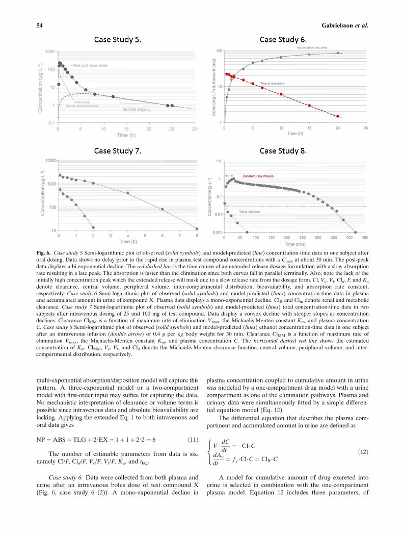
multi-exponential absorption/disposition model will capture thispattern. A three-exponential model or a two-compartmentmodel with first-order input may suffice for capturing the data.No mechanistic interpretation of clearance or volume terms ispossible since intravenous data and absolute bioavailability arelacking. Applying the extended Eq. 1 to both intravenous andoral data gives

NP ¼ ABSþ TLGþ 2⋅EX ¼ 1þ 1þ 2⋅2 ¼ 6 ð11Þ

The number of estimable parameters from data is six,namely Cl/F, Cld/F, Vc/F, Vt/F, Ka, and tlag.

Case study 6. Data were collected from both plasma andurine after an intravenous bolus dose of test compound X(Fig. 6, case study 6 (2)). A mono-exponential decline in

plasma concentration coupled to cumulative amount in urinewas modeled by a one-compartment drug model with a urinecompartment as one of the elimination pathways. Plasma andurinary data were simultaneously fitted by a simple differen-tial equation model (Eq. 12).

The differential equation that describes the plasma com-partment and accumulated amount in urine are defined as

V⋅dCdt

¼ −Cl⋅CdAu

dt¼ f e⋅Cl⋅C ¼ ClR⋅C

8><>: ð12Þ

A model for cumulative amount of drug excreted intourine is selected in combination with the one-compartmentplasma model. Equation 12 includes three parameters, of

Fig. 6. Case study 5 Semi-logarithmic plot of observed (solid symbols) and model-predicted (line) concentration-time data in one subject afteroral dosing. Data shows no delay prior to the rapid rise in plasma test compound concentrations with a Cmax at about 30 min. The post-peakdata displays a bi-exponential decline. The red dashed line is the time course of an extended release dosage formulation with a slow absorptionrate resulting in a late peak. The absorption is faster than the elimination since both curves fall in parallel terminally. Also, note the lack of theinitially high concentration peak which the extended release will mask due to a slow release rate from the dosage form. Cl, Vc, Vt, Cld, F, and Ka

denote clearance, central volume, peripheral volume, inter-compartmental distribution, bioavailability, and absorption rate constant,respectively. Case study 6 Semi-logarithmic plot of observed (solid symbols) and model-predicted (lines) concentration-time data in plasmaand accumulated amount in urine of compound X. Plasma data displays a mono-exponential decline. ClR and Clm denote renal and metabolicclearance. Case study 7 Semi-logarithmic plot of observed (solid symbols) and model-predicted (lines) total concentration-time data in twosubjects after intravenous dosing of 25 and 100 mg of test compound. Data display a convex decline with steeper slopes as concentrationdeclines. Clearance ClMM is a function of maximum rate of elimination Vmax, the Michaelis-Menten constant Km, and plasma concentrationC. Case study 8 Semi-logarithmic plot of observed (solid symbols) and model-predicted (lines) ethanol concentration-time data in one subjectafter an intravenous infusion (double arrow) of 0.4 g per kg body weight for 30 min. Clearance ClMM is a function of maximum rate ofelimination Vmax, the Michaelis-Menten constant Km, and plasma concentration C. The horizontal dashed red line shows the estimatedconcentration of Km. ClMM, Vc, Vt, and Cld denote the Michaelis-Menten clearance function, central volume, peripheral volume, and inter-compartmental distribution, respectively.


which Cl occurs in both the plasma and cumulative urineequations. Therefore, try whenever possible to utilize asmany sources of data (such as plasma concentrations andurine amounts) simultaneously when fitting a model to thedata to increase accuracy and precision of the parameterestimates. The model for cumulative amount in urine has avery robust model structure and generally allows accurateand precise estimation of fe or ClR in our experience.

The key features of this analysis are a combined plasmaconcentration and urinary excretion model that was simulta-neously fit to two sources of time series. Key patterns aremono-exponential decline in plasma and a smooth first-orderrise in cumulative amounts in urine. Volume and clearanceare related to both datasets. Applying the extended Eq. 1 toboth intravenous and urinary data gives

NP ¼ 2⋅EXþ PE ¼ 2⋅1þ 1 ¼ 3 ð13Þ

The number of estimable parameters from data is three,namely Cl, V, and ClR or fe.

Case study 7. A convex decline is observed in twoconcentration-time profiles after intravenous dosing of twodoses to two individuals (Fig. 6, case study 7 (2)). This patternshows a typical signature that cannot be modeled by addingmore exponential terms. Since the slope of decline gets shallowerin both subjects the higher the plasma concentration becomes, itsuggests some kind of nonlinearity in possibly the eliminationprocess. One typically would think of capacity-limited elimina-tion (often called dose or concentration-dependent elimination),but if total concentrations are displayed, this could also beexplained by saturable plasma protein binding. In this case study,we fit a model with capacity-limited (Michaelis-Menten) elimi-nation to the data. Note that the terminal portions of theconcentration-time courses have different slopes. Dose-normalized concentrations displayed the same initial concentra-tion but deviated from each other during the remainingconcentration-time courses. We suggest that volume V andmaximum rate of elimination Vmax are the same for the twosubjects but that their Km values differ since total concentration-time data are available for this highly plasma-bound testcompound. The underlying assumption is that Km is moreaffected by plasma protein binding differences across subjectsthan Vmax. We also tested using the same Km but different Vmax

parameters for the two subjects but that failed to produce anacceptable fit (see Gabrielsson and Weiner, 2010, for a detaileddescription of the analysis).

The plasma equation following intravenous administra-tion is written as

V⋅dCdt

¼ −ClMM⋅C

ClMM ¼ Vmax

Km þ C

8><>: ð14Þ

C and ClMM are the plasma concentrations and Michaelis-Menten type of capacity-limited clearance, respectively, andVmax

and Km are maximum rate of elimination and the Michaelis-Menten constant. It is theMichaelis-Menten expression in Eq. 14

that allows the model to capture the lack of superposition acrossdoses and the time-dependent half-life.

The key features of these patterns are analysis of twoconcentration-time profiles that both display a convex shapeof decline. Dose-normalized concentrations superimpose onlyat C(0) and deviate beyond that time point. A multi-phasicconcave pattern was observed which typically occurs innonlinear capacity-limited elimination. Both profiles declinedin a linear fashion at low plasma concentrations. A successfulattempt was made to simultaneously fit the two time courseswith a common value for both subjects for the Vmax andvolume V parameters but two different Km values. Applyingthe extended Eq. 1 to both intravenous time courses gives

NP ¼ 2⋅EXþNL1 þNL2 ¼ 2⋅1þ 1þ 1 ¼ 4 ð15Þ

NL1 and NL2 are the observed different nonlinearplacements in the two datasets that Eq. 14 was simultaneouslyfitted to. The number of estimable parameters from data isfour, namely Vmax, V, Km1, and Km2.

Case study 8. The kinetics of ethanol was characterizedfollowing a 30-min constant rate intravenous infusion (Fig. 6,case study 8 (5)). A number of volunteers were infusedintravenously with a dose of 0.4 g ethanol per kg body weight.Plasma samples were obtained for 7 h. Ethanol displayedcapacity-limited clearance and a volume of distributionequal to total body water. This problem highlights someof the complexities in modeling multi-compartment dispo-sition with nonlinear capacity-limited elimination. Fordetails about study design and a review of ethanol kinetics,see Norberg et al. (5,6).

The constant rate infusion of ethanol occurred over30 min. Post-infusion data display initially a small concaveshape followed by a slow extended convex decline withsteeper slopes as concentration declines. The rapid post-infusion concave bend suggests an additional compartmentbeyond plasma that ethanol distributes into. It is well knownthat ethanol distributes into total body water (a 40-L volumein a 70-kg person). The top portion of the second phase afterthe stop of infusion is shallow and starts to bend down with asteeper slope as concentrations decline. This convex bendsuggests some kind of nonlinearity that excludes bindingchanges. Saturation of the metabolizing enzymes are wellknown for ethanol above 30 μg L−1. Therefore, a Michaelis-Menten type of expression of clearance was included into themodel (Eq. 16).

Vc⋅dCdt

¼ In−Cl⋅C−Cld⋅C þ Cld⋅Ct

Vt⋅dCt

dt¼ Cld⋅C þ Cld⋅Ct

Cl ¼ Vmax

Km þ C

8>>>>>>><>>>>>>>:

ð16Þ

The model has five parameters (Vmax, Km, Cld, Vc, and Vt)and three constants (two doses, one duration of infusion). We fitthe data simultaneously.


The key features of this analysis are initially a bi-exponential concave decline after an intravenous constant rateinfusion, followed by nonlinear capacity-dependent eliminationthat transgresses into a convex downward bend. The terminalportion of the curve displays a linear mono-exponential decline.The bi-exponential behavior suggests a two-compartmentstructure and the nonlinearity a Michaelis-Menten type ofelimination. If we then apply the extended Eq. 1 with necessaryparameters for the present dataset, we get Eq. 17

NP ¼ 2⋅EXþNL ¼ 2⋅2þ 1 ¼ 5 ð17Þ

which gives five parameters that are estimable from data(Cld, Vc, Vt, Vmax, and Km).

Case study 9. Three oral doses of compound Y weregiven to the same subject at three different occasions. No lagtime was observed but there was a peak shift in the plasmaconcentrations as the dose increased (Fig. 7, case study 9, redvertical lines (2)). The post-peak events become more andmore shallow as dose increases. The three time courses fall off ina linear parallel fashion as concentrations approach less than5–10 μg L−1. The pharmacokinetics may be characterized bya one-compartment model with first-order absorption andsaturable elimination. The peak shift may be due to saturableabsorption or saturable elimination. Provided complete absorp-tion (100% bioavailability) or saturable absorption, the dose-normalized areas would superimpose. However, in this casestudy, the dose-normalized areas do not superimpose suggestingthat nonlinear elimination causes the peak shift.

The equations corresponding to the concentration inplasma are written as

Inputpo ¼ F⋅Ka⋅Dosei⋅e−Ka⋅t

V⋅dCdt

¼ Inputpo−ClMM⋅C

ClMM ¼ Vmax

Km þ C

8>>>>>><>>>>>>:

ð18Þ

The key features of this analysis are peak shifts withincreasing oral doses with tmax at 40, 50, and 100 min after thelow, intermediate, and high doses, respectively. The peakconcentration is followed by an apparent nonlinear andseemingly flatter portion of the curve at the highest dose.The terminal decline below 10 μg L−1 is mono-exponential.Dose-normalized areas do not superimpose which suggestseither nonlinear bioavailability or nonlinear elimination. If wethen apply the extended Eq. 1 with necessary parameters forthe present dataset, we get

NP ¼ ABSþ 2⋅EXþNL ¼ 1þ 2⋅1þ 1 ¼ 4 ð19Þ

four parameters that are estimable from data (Ka, V, Vmax,and Km).

Case study 10. Three oral solutions of a test compoundwith increasing doses to human subjects displayed a nonlinearpattern at the peak concentrations (Fig. 7, case study 10 (2)).The initial rise of the plasma concentration is very rapid with

a peak concentration occurring within 10 min after dosing at thefirst observation. Not only was a peak shift observed withincreasing doses but also a flat portion at the highest dose lastingfor about 100 min. Dose-normalized areas, obtained from non-compartmental analysis, superimposed, suggesting that theextent of absorption is complete but the rate is saturable. Thecompound utilizes a transporter system for endogenous com-pounds like amino acids, hormones, and other food ingredients.Data also displays a bi-exponential (concave) decline at concen-trations below 100 μg L−1. Figure 7 (case study 10) shows thehigh-resolution data from a single individual. The data pattern isinteresting as it displays a brief period with absorption rate-limited kinetics during the first 100 min, and then displaysdisposition rate-limited kinetics in the terminal phase.

The function of the concentration in the central com-partment is written as

In ¼ Vmax⋅Ag

Km þAg

Vc⋅dCdt

¼ In−Cl⋅C−Cld⋅C þ Cld⋅Ct

Vt⋅dCt

dt¼ Cld⋅C þ Cld⋅Ct

8>>>>>><>>>>>>:

ð20Þ

where Vmax, Ag, and Km represent the maximum transportrate (μg min−1), amount in the gut compartment (μg), and theMichaelis-Menten constant (μg) at which half-maximal inputrate operates. The model has five parameters (Vmax, Km,Cld, Vc, and Vt) and three constants (three doses). The threeconcentration-time courses are fit simultaneously. It is thenonlinear input function in Eq. 20 that allows us to capturethe nonlinear absorption pattern.

The key features of this analysis are an initial rapid rise inplasma concentrations with a peak within 10min after dosing forthe lowest dose followed by peak shifts inCmax and an extendedplateau at the highest dose. The time courses display bi-exponential decline at concentrations below 100 μg L−1. Dose-normalized areas-under-the plasma concentration curves super-impose suggesting complete absorption and linear elimination.If we then apply the extended Eq. 1 with necessary parametersfor the present dataset, we get

NP ¼ ABSþ 2⋅EXþNL ¼ 1þ 2⋅2þ 1 ¼ 6 ð21Þ

However, there are only five parameters that are estimablefrom data (Vmax and Km, Cld/F, Vc/F, Vt/F,). Since we apply anonlinear transport to the absorption process, both ABS andNL relate to the same process.

Case study 11. Estradiol was given as a rapid intravenousinjection to a post-menopausal woman. Estradiol concentra-tions in plasma were measured prior to dosing and during32 h post-dosing (Fig. 7, case study 11 (2)). A two-compartment model with endogenous turnover and clearancewas fit to the data. Initial parameters were obtained bygraphical methods.

The bi-exponential decline observed in Fig. 7 (case study 11)displays two distinct phases before the estradiol plasma concen-tration asymptotically approaches the baseline concentration.The two phases are separated by a concave bend in the curve.


The bi-exponential decline approaching a baseline can bedescribed by a system of differential equations (Eq. 22). Therelationship between the concentration C and the rate of changedC/dt in plasma and tissue can be expressed mathematically as asystem of two differential equations for a two-compartmentmodel with first-order kinetics, when drug is administered as abolus dose as follows:

Vc⋅dCdt

¼ Inputbolus þ Rin−Cl⋅C−Cld⋅C þ Cld⋅Ct

Vt⋅dCt


8><>: ð22Þ

dC/dt and dCt/dt are the rate of change of test compoundin plasma and tissue, C is the plasma concentration, Ct the

tissue concentration, Cl plasma clearance, Vc central volume,Vt peripheral volume, and Cld the inter-compartmentaldistribution parameter. Cld has the units of volume per time(mL min−1 or L min−1) and is related to transport via bloodflow, transporters, and diffusion/convection forces. Inputscand Rin denote the exogenous bolus dose and endogenoussecretion of estradiol, respectively. Rin is a model parameterthat will be estimated together with Cl, Cld, Vc, and Vt whenfitting the model to the data. Here, we assume the endoge-nous production of estradiol is constant during the observa-tional time period.

The key features of this analysis are bi-exponentialdecline in plasma, a baseline at 20 pmol L−1, and a shorteffective half-life. Baseline subtracted data would reveal anapparent bi-exponential decline. Extending the reasoning of

Fig. 7. Case study 9 Semi-logarithmic plot of observed (solid symbols) and model-predicted (lines) concentration-time data in one subject afterthree different doses of test compound Y. F, Ka, V, Vmax, and Km denote the bioavailability, absorption rate constant, volume of distribution,maximum metabolic rate, and Michaelis-Menten constant, respectively. Case study 10 Semi-logarithmic plot of observed (symbols) and model-predicted (lines) concentration-time data after oral dosing of a test compound that utilizes an endogenous transporter route. The oral profilesdisplay nonlinear absorption with a peak shift in Cmax with increasing doses. A typical bi-phasic decline is shown post-peak and below plasmaconcentrations of approximately 100 μg L−1. Note the flip-flop situation during the first 120 min at the highest dose where rate of elimination isconfounded by absorption. F, Vmax, Km, Vc, Vt, Cld, and Cl denote bioavailability, maximum transport rate, the Michaelis-Menten constantrelated to the saturable absorption process, central volume, peripheral volume, inter-compartmental distribution, and clearance, respectively.Case study 11 Semi-logarithmic plot of concentration-time data obtained from a post-menopausal woman who received a rapid injection of10 nmol of estradiol. An apparent bi-exponential decline approaches a baseline at approximately 20 pmol L−1. This behavior corresponds to atwo-compartment system (right) with parallel endogenous (turnover, synthesis) and exogenous (intravenous bolus) input of estradiol. There isabsolutely no need to subtract baseline values from experimental data in order to model the data. Cl, Vc, Vt, Cld, and turnover rate denoteclearance, central volume, peripheral volume, inter-compartmental distribution, bioavailability, and endogenous turnover rate, respectively.Case study 12 Observed (filled circles) and model-predicted (line) concentration-time data of growth hormone after a subcutaneous dose of40 μg kg−1. The shaded area shows the area corresponding to exogenous input of growth hormone. Turnover, Cl, V, F, and Ka denote theendogenous turnover rate, clearance, volume of distribution, bioavailability, and absorption rate constant, respectively. Data are displayed on alinear scale which more clearly highlights the key features.


Eq. 1, we would suggest that an additional parameter isneeded in the model and that is the baseline information BL.Applying Eq. 1 with the baseline information included givesEq. 23

NP ¼ 2⋅EXþ BL ¼ 2⋅2þ 1 ¼ 5 ð23Þ

which corresponds to five parameters (Rin, Cl, Cld, Vc, and Vt)to be estimated.

Case study 12. This case study of pattern recognitiondemonstrates the turnover concept including turnover rateand turnover time. A healthy volunteer received a 40 μg kg−1

dose D of growth hormone subcutaneously (sc). The plasmaconcentrations of growth hormone, which were measuredbefore and during 72 h post-dosing, are shown in Fig. 7 (casestudy 12 (2)) together with predicted concentrations. Thedata pattern includes a pre- and post-dose baseline concen-tration, a plasma concentration peak at about 2 h, and a rapidreturn back to baseline concentrations within 24 h.

The pre-dose concentration was 32 μg L−1. We willestimate the basic kinetic parameters such as clearance Cl/F(denoted Cl), volume of distribution V/F (denoted V), andabsorption rate constant Ka. The underlying differentialequation that takes endogenous turnover rate Rin andelimination Cl, together with the subcutaneous application,into account is

Insc ¼ Ka⋅FDsc⋅e−Ka⋅t

V⋅dCdt

¼ Rin þ Insc−Cl⋅C

8><>: ð24Þ

We assume that the baseline concentration (initialcondition) can be written as Rin/Cl (synthesis or turnover ratedivided by Cl), and that F is equal to unity.

The key features of this analysis are bi-exponential input/output, a baseline at 32 μg L−1, and a short effective half-life.Extending the reasoning of Eq. 1, we would suggest that anadditional parameter be added to the model and that isbaseline information BL. Applying Eq. 1 with the baselineinformation included gives Eq. 25

NP ¼ 2⋅EXþABSþ BL ¼ 2⋅1þ 1þ 1 ¼ 4 ð25Þ

which corresponds to four parameters (Rin, Cl/F, V/F, Ka) tobe estimated.

Case study 13. This case study covers the analysis oftarget-mediated disposition TMDD. Assuming high affinity ofligand to target, we provide a quantitative solution of ligand,soluble target, and ligand-target complex after a rapidintravenous injection dosing of the ligand. Data on the ligandconcentration-time courses after four rapid intravenousinjection doses are shown in Fig. 8 (case study 13 (2,7)).

The TMDD model is schematically depicted in Fig. 8(case study 13). The typical shapes of a plasma concentration-time course that TMDD displays start with a rapid declinewithin the minute to hour range due to the second-order

reaction between ligand and soluble target. This phase isextended in both the concentration and the time range withdiminishing doses. Remember that the rate process –kon L Ris dependent on both ligand and target concentrations andtheir relative sizes. The initial drop may easily be missed if thefirst plasma sample is 12–24 h post-dose. Then, the curvedisplays a concave bend towards a slower decline. One oftenhas first-order linear (dose-proportional) kinetics at higherexposure of ligand. The concentration-time course displaysbi-exponential decline at higher doses after intravenousdosing because the target, as a clearing route, is saturated.

The third typical phase is then a convex bend downwardwith a shorter apparent half-life as we approach lowerconcentrations. This phase is where TMDD starts to be ofimportance. The kinetics is now nonlinear. The appearance ofthe downward bend will occur at the same ligand concentra-tions independently of ligand dose. Throughout this phase,the target route of elimination is more or less saturable, butless saturable at low concentrations and therefore a moredominating clearing route in that concentration range.

Finally, the ligand enters a slower terminal phase, againafter a concave bend, with a longer apparent half-life. Thisphase is very much governed by the elimination rate constantke(RL) of complex RL and in some instances also byunspecific distribution (Cld, Vt) of ligand.

The disposition of the antibody (ligand, L) is describedby a two-compartment non-specific disposition model coupledto a zero-order production first-order loss target pool R.Ligand and target forms a complex RL via a second-orderprocess. The complex can either be degraded into ligand andtarget via the first-order koff process or be irreversibly lost viake(RL) (first-order internalization or sink parameter). Thecombination of the second-order formation and first-orderloss of complex makes the system nonlinear.

Vc⋅dCL

dt¼ InputL−ClL⋅CL−Cld⋅CL þ Cld⋅Ct

Vt⋅dCt

dt¼ Cld⋅CL−Cld⋅Ct

dRdt

¼ kin−kout⋅R−kon⋅CL⋅Rþ koff⋅CRL

dCRL

dt¼ kon⋅CL⋅R−koff⋅CRL−ke RLð Þ⋅CRL

8>>>>>>>><>>>>>>>>:

ð26Þ

CL, inputL, ClL, Cld, kon,R, koff,CRL,CT, andVt denote theligand concentration, input of ligand, first-order clearance ofligand, inter-compartmental distribution of ligand, second-orderrate constant for the ligand-target interaction, target level, first-order dissociation rate constant of the ligand-target complex,complex concentration, concentration of ligand in tissue due tonon-specific distribution, and the volume of distribution of non-specific distribution of ligand. The ke(RL) is the first-order rateconstant of irreversible removal of the complex.

It should also be remembered that the concentration-time courses similar to those following intermediate dosesmay in some instances also be observed for therapeuticproteins that do not undergo TMDD but exhibit theformation of clearing anti-drug antibodies (ADA) due to animmunological reaction (8). This usually takes some time todevelop and is sometimes seen after repeated dose adminis-tration of, for example, monoclonal antibodies.


The number of parameters NP which may be calculatedbased on the observed pattern in Fig. 8 depends on the numberof apparent exponentials EX (=3 apparent linear phases in thesemi-logarithmic diagram) visible in the plasma concentration-time profile, the number of tissue spaces or binding proteins TS(=1 target) analyzed, and the number of visible nonlinearfeatures NL (=1) in the data. This information results in

NP ¼ 2⋅EXþ 2⋅TSþNL ¼ 2⋅3þ 2⋅1þ 1 ¼ 9 ð27Þ

This gives nine parameters based on the very simplerelationship in Eq. 27. Still, additional concentration-timedata on target (=2 parameters) and complex (=3 parameters)

need to be included to improve the precision of certainparameters. See Peletier and Gabrielsson (7) for a thoroughdiscussion of this dataset.

Case study 14. This case study illustrates how the timecourse of a drug can change upon repeated dosing when theenzymes responsible for its metabolism are induced. A studywas conducted to see if the drug metabolizing enzymes ofnortriptyline NT are inducible by pentobarbital PB by ahetero-induction process. NT was therefore administeredorally as a 10-mg dose every 8 h for a period of 29 days(696 h). After 9 days (216 h), treatment with PB (inducer)was initiated and lasted for 12.5 days (300 h), i.e., until

Fig. 8. Case study 13 Semi-logarithmic plot of observed (symbols) and TMDD model-predicted concentrations (solid lines) at four differentdoses of 1.5, 5, 15, and 45 mg kg−1 after rapid intravenous injections of a monoclonal antibody. Note that the ligand displays a multi-compartment target-mediated disposition pattern that changes in shape with the change in ligand exposure (dose). The plot also shows theplasma target baseline concentration R0, the estimated Michaelis-Menten constant Km, and the dissociation constant Kd (7). Case study 14Observed (filled circles) and predicted (solid line) plasma concentrations of nortriptyline (10 mg tid) before (A, 0–216 h), during (B, 216–516 h),and after (C, 516–700 h) pentobarbital Pb treatment. The horizontal bar represents the induction period. Data are displayed on a Cartesianscale due to the limited concentration range which more clearly highlights the key features. Case study 15 Observed (filled symbols) and modelpredictions (lines) of parent compound (solid lines) and metabolite (dashed lines) plasma concentration-time data. Note the change in half-lifewith increasing concentrations. The intravenous bolus doses of drug were 10, 50, and 300 μmol kg−1. The red solid lines are included as a visualhelp with respect to how the slope changes across low and high exposure data. Note the separation between parent C and metabolite CM

concentrations with increasing doses of parent compound. C, Vc, Vt, Cld, ClM, Vmax, Km, VM, and kME denote the parent plasma concentration,central volume, peripheral volume, inter-compartmental distribution, metabolic clearance of parent compound, maximum metabolic capacity,the Michaelis-Menten constant, volume of distribution of metabolite, and elimination rate constant of metabolite, respectively. Case study 16Observed (filled symbols) and model-predicted (lines) concentration-time data following an oral dose of 20 mg of compound A. The zero-orderabsorption model predicts a discontinuous line at approximately 4 h. The gray horizontal line illustrates the length of constant rate drug inputTabs. The first-order model misses the peak concentration and displays systematic deviations between observed and model-predictedconcentrations. Note the delayed absorption with a maximum observed plasma concentration at 4 h. Ka, Tabs, V (actually V/F), and K denotethe absorption rate constant, duration of the zero-order absorption, volume of distribution, and elimination rate constant, respectively. Data aredisplayed on a Cartesian scale due to the limited concentration range which more clearly highlights the key features.


21.5 days (516 h) after the start of NT administration. Theobserved and predicted plasma concentration-time course ofNT before, during, and after treatment with inducer isdepicted in Fig. 8 (case study 14 (9)).

V ⋅dCdt

¼ Inputpo−C l tð Þ ⋅ CInputpo ¼ Dpo⋅ Ka⋅ e−Ka⋅t

Cl tð Þ ¼ Clinduced− Clinduced−Cluninducedð Þ⋅e−kout⋅t

8>><>>:

ð28Þ

where V, Cl(t), Inputpo, C, Dpo, Ka, Clinduced, Cluninduced, andkout denote volume of distribution, time-dependent clearanceof nortriptyline, nortriptyline plasma concentration, oralnortriptyline dose, absorption rate constant, induced clearance(from pentobarbital treatment), uninduced (pre-pentobarbitaltreatment) clearance, and fractional turnover rate of theinducible enzyme, respectively. Two hundred hours after thestart of the study pentobarbital treatment was initiated (Fig. 8,case study 14, A). During induction, the half-life is continuouslyshortened (10 h) resulting in a reduced time to the induced steadystate (Fig. 8, case study 14, B) in contrast to the return from theinduced state (Fig. 8, case study 14, C) when Cl/F constantlydiminishes and the corresponding half-life returns back to its pre-induction value. The exposure to nortriptyline is also more thanhalved during induction. Due to the constantly changing clear-ance (increasing) and half-life (decreasing), the time to steadystate during the induction period is extended in spite of the factthat half-life is getting shorter (10 h) than before induction (25 h).The principle of three to four half-lives until steady state is notapplicable for a system where half-life is constantly changing.

Case study 14 has demonstrated the consequences ofinduction of the responsible metabolizing enzymes by anothercompound (hetero-induction by pentobarbital on nortriptylinemetabolism). Induction or inhibition by the parent compounditself or a metabolite is also possible (e.g., carbamazepine (10)).This is manifested as a lower (induction, causing the half-life todecrease) or higher (inhibition, causing the half-life to increase)exposure to the test compound over time. Saturable tissuebinding can also lead to a lack of predictive power by single-dosedata. It is therefore suggested that chronic indications requirechronic dosing, and consequently pharmacokinetic assessmentmust be based on repeated dose information.

The key features of these patterns are steady-stateexposure data after oral administration of nortriptyline whichthen diminishes by means of the induction process (throughvalues and a complete time course peri-induction) and thenshows a post-induction return towards pre-induction steadystate. Applying Eq. 1 gives Eq. 29

NP ¼ 2⋅EXþABSþNL ¼ 2⋅1þ 1þ 1 ¼ 4 ð29Þ

which corresponds to four parameters (kout, Cl/F, V/F, Ka) tobe estimated.

Case study 15. The concentration of drug A and metabo-lite M were measured in plasma at different times afterintravenous bolus doses of 10, 50, and 300 μmol kg−1. Figure 8(case study 15 (2)) depicts the experimental concentration datafor drug (solid lines) and metabolite (dashed lines).

The parent compound data show a bi-exponentialdecline with a concave curvature at about 30 min. The half-life of parent compound increases with increasing concentra-tions (doses). Notice that the metabolite peak concentrationincreases in a less than proportional manner and occurs laterin time with increasing doses. The slope of the initial orintermediate portion of the plasma concentration-time pro-files increases with dose and the separation of the parent andmetabolite-time courses increases with higher doses. Theterminal portion obeys first-order kinetics and should there-fore be independent of dose (concentration). This patternsuggests a two-compartment system of differential equationsfor the parent compound (drug) with saturable elimination.The nonlinear elimination from parent becomes nonlinearformation input to a one-compartment metabolite (M) model.The three-compartment system is given by Eq. 30. In thismodel, an intravenously administered drug is fully convertedto metabolite through its metabolic clearance and thenexcreted as the metabolite.

The system of differential equations of this model is

Vc⋅dCdt

¼ In−ClM⋅C−Cld⋅C þ Cld⋅Ct

ClM ¼ Vmax

Km þ C

Vt⋅dCt


VM⋅dCM

dt¼ ClM⋅C−ClME⋅CM

8>>>>>>>>><>>>>>>>>>:

ð30Þ

The ClME parameter is the first-order clearance param-eter of the metabolite. Note that ClM is the metabolicclearance of the drug, which is the same as the formationclearance of the metabolite. ClM will be more and moresaturated, the higher the doses are of the parent compound.This results in formation-limited elimination of the metaboliteand is observed as a flatter concentration-time course (longerapparent half-life of metabolite) at higher exposure to theparent compound.

The key features of this analysis are three bi-exponentialtime courses after intravenous dosing of parent compound.Data also contains information about the rise and fall of ametabolite in plasma which occurs via a saturable process. Inthis case, we have two different data sources which allow us toestimate

NP ¼ 2⋅EXþNLþMTB ¼ 2⋅2þ 1þ 2⋅1 ¼ 7 ð31Þ

seven parameters (Vmax, Km, Cld, Vc, Vt, VME, and ClME).

Case study 16. A volunteer was given 20 mg orally of ahighly polar drug (Fig. 8, case study 16 (2)). Data show aninitial time delay followed by a late peak at about 4 h and apost-peak mono-exponential decline. The objectives of thisexercise are therefore to identify and fit the most suitable oftwo different types of absorption models to a dataset obtainedafter extravascular dosing with compound A. One is a first-order model including a lag time, the other is a zero-orderinput model.


The absorption process from the gastrointestinal tract iscomplex and involves several processes such as disintegrationof the tablet, dissolution of the drug into the gastric fluids,gastric emptying, diffusion across the gut wall to mention justa few. In general, absorption processes are assumed to occurby means of a first-order process, although there areexceptions. Under certain conditions, it has been found thatabsorption of compounds is better described by zero-orderkinetics. The first- and zero-order input models are shown inEq. 32.

V ⋅dCdt

¼ Input rate−ClF

⋅C

First‐order input rate ¼¼ 0 when t < tlagelse¼ Ka⋅Dpo⋅e−Ka⋅ t−tlagð Þ

8<:

Zero‐order input rate¼ Dpo

Tabswhen t < Tabs

else¼ 0

8><>:

8>>>>>>>>>>><>>>>>>>>>>>:

ð32Þ

where Tabs is the assumed duration of zero-order input.Equation 31 is equivalent to a one-compartment continuousinfusion model where the duration of the infusion Tabs isestimated as a parameter.

In this case study, there is a distinct difference betweenthe zero-order input (model of choice) and first-order inputmodels (systematic deviations throughout the model-predicted concentration-time course), which is already shownin the function plots. In other words, the latter model isnot an option and there is no need to extend the analysisto inspection of residuals or use other tools in thestatistical battery (parameter precision, correlation, F test)(see Gabrielsson and Weiner (2) for a discussion).

The key pattern of this dataset is a somewhat delayedonset of absorption, a concentration maximum at about 4 h,and a mono-exponential decline post-peak.

Applying Eq. 1 gives Eq. 33

NP ¼ 2⋅EXþABSþ TLG ¼ 2⋅1þ 1þ 1 ¼ 4 ð33Þ

which corresponds to four parameters (tlag or Tabs and Cl/F,V/F, Ka) to be estimated.

DISCUSSION

Pattern recognition is a pivotal aspect of exploratorydata analysis when modeling pharmacokinetic and pharma-codynamic data. Therefore, a rigorous strategy is essential fordissecting the patterns that concentration-time profiles reveal.As an alternative solution, one may utilize a set of points toconsider that specifically addresses number of phases, convexor concave bending, time lags, peak shifts, baseline behavior,effective half-lives, dose-normalized areas, concentrationplateaus, and similar phenomena. Pattern recognition hasalso been proposed for interpreting results of drug-druginteractions. BA quicker and better understanding about theprocesses, which dominate a DDI, has been achieved using

this approach by focusing on integration of all informationavailable and mechanistic interpretation^ (1).

The application of the extended Eq. 1 has beensuccessful for the presented case studies but should in generalbe used cautiously and only from an exploratory point ofview. One may decipher other characteristics of the data byfor example simultaneously fitting several time courses.

Considerations and Methodologies for Comparisonand Experimental Design

We advocate an iterative process for discriminationbetween rival models. This is done by starting with a simplermodel (say bi-exponential or no lag time model), fit thatmodel to the data, perform a thorough residual analysis (2),and look at other goodness-of-fit criteria (objective functionvalue,Akaike information criteria, etc.) together with parametercorrelation and precision. The next step is then to systematicallyextend the model (adding an exponential term or a lag time ifnecessary), refit the updated model to the data, and inspect theresiduals in combination with the statistical battery (goodness-of-fit, parameter precision, parameter correlation). In somecases, an F test analysis may be a final check of the model ofchoice, although the residual analysis (again visual inspection oftransformed data) is, in our experience, a powerful approach inmodel selection. The most parsimonious model is preferable inmost modeling situations.

We advocate an iterative approach to practical experi-mental design. Start by running a pilot study with a singledose, a few animals, and logarithmic spacing of data in time.Then fit a model to the data to get an acceptable fit aspossible without overdoing the analysis. Simulate the newdesign(s) with the model using the final parameter estimatesfrom the pilot study. Propose alternative doses, alternativesampling time points, and/or a repeated dose design ifnecessary. Run the study and collect data according to reviseddesign. Now fit all data from pilot and redesigned studysimultaneously. If the model mimics all data, it is probably arelatively robust model. We commonly use this iterativeapproach (running a dose-range finding limited animal/sample approach) prior to the more expensive repeated dose(e.g., 1-, 3-, or 12-month safety) studies. There are severalreal-life case studies in Gabrielsson and Weiner wheresimultaneous fitting of data from two or more (incomplete)experiments have proven to be useful (2). One may also wantto consider sparse sampling in combination with a mixed-effects modeling approach to save both animals and cost. Themixed-effects modeling approach has of course great poten-tial but is beyond the focus of this report.

Some General Points to Consider with Respect to VisualInspection of Data

Data collected from intravenous dosing are used forassessment of the disposition (binding, distribution, elimination)of a test compound in plasma and urine. Central themes of whatone observes in data patterns are the following:

(1) the number of exponential phases in a semi-logarithmic concentration-time plot corresponds tothe number of compartments in a linear mammillary


compartment system after a rapid bolus injection ora short constant intravenous infusion.

Number of compartments ¼ Number of phases in plasma

ð35Þ

(2) Nonlinearities such as capacity-, time-, binding-, andflow-dependent phenomena (Eq. 36) are revealedby convex bends in the concentration-time profile(see case studies 7–9, 13, and 15), which suggestthat one or more nonlinear terms are needed inthe model. Also, dose normalize the concentration-time curves and check whether they superimpose.A set of nonlinear expressions are collated below.

Nonlinearities ¼

Capacity Cl ¼ Vmax

Km þ C

Time Cl tð Þ ¼ Vmax tð ÞKm þ C

Binding f u ¼ Cu þKd

Cu þKd þ n⋅ PT½ �Flow Cl ¼ QH⋅ f u⋅Clint

QH þ f u⋅Clint

ClH ¼ QH;B⋅ f u⋅Cluint;H

QH;B þ f u⋅Cluint;H=CB

CP

� �

8>>>>>>>>>>>>>>>>><>>>>>>>>>>>>>>>>>:

ð36Þ

Vmax(t), Kd, n, [PT], QH, and Clint denote the time-dependent maximum metabolic capacity, affinityconstant between drug and protein, number ofbinding sites on the protein, protein concentration,hepatic blood flow, and intrinsic clearance, respec-tively. ClH,QH,B, fu, Clu int,H,CB, andCp are the hepaticblood clearance, hepatic blood flow, free fraction inplasma, unbound hepatic intrinsic clearance, totalblood concentration, and total plasma concentration,respectively (11).

(3) Extravascular data (oral data or data from alterna-tive extravascular dosing) reveal time delays (tlag),rate (Ka), and extent (F) of absorption, or evencapacity-limited (Vmax, Km) input that impacts theonset of absorption, absorption rate, the AUC, andpeak shifts in Cmax/tmax when two or more doses aregiven, respectively. Useful expressions related toabsorption profiles are shown in Eq. 37.

Absorption ¼Input rate F⋅Dosepo⋅e−Ka⋅ t−tlagð ÞExtent F ¼ f a⋅ fHCapacity input rate ¼ Vmax

Km þAg

8>><>>:

ð37Þ

Ag, fa, and fH denote the amount at the absorptionsite (e.g., in the gut), fraction absorbed into blood,and fraction that passes through the liver, respec-tively. All other parameters are explained above.One should remember, however, that data from onlythe oral route may confound the interpretation of

slopes, clearance, and volume terms. A potentialsolution to this is to utilize iv and oral datasimultaneously.

(4) Baseline concentrations of endogenous compoundsneed to be considered by adding some productionterm (turnover rate) simultaneously with the clear-ance parameter

Baseline ¼ Turnover rateCl

ð38Þ

When baseline values are observed for exogenouscompounds one does not have to consider anendogenous turnover rate but rather setting theinitial condition of the state variable(s) to themeasured pre-dose value.

(5) Measurements in other body tissues and fluids, forexample, urinary data, may contribute to the estima-tion of either renal clearance ClR or fraction excretedvia urine fe

dAu

dt¼ ClR⋅C ¼ f e⋅Cl⋅C ð39Þ

where dAu/dt and C are the rate of excretion of druginto urine and the plasma concentration.

The objective of this communication has been to focuson visual inspection of Bshapes^ of concentration-timeprofiles in the exploratory analysis of pharmacokinetic data.We have tried to decompose the shapes and to systematicallyinterpret what determines the rise, intensity, and decline ofexposure. This approach may serve as a road map to patternrecognition of concentration-time data.

Additional sources of data from two or more doses,urine, metabolite information, and repeated dose data should,whenever possible, be considered as part of a simultaneousfitting procedure.

REFERENCES

1. Duan JZ. Drug-drug interaction pattern recognition. Drugs R D.2010;10(1):9–24.

2. Gabrielsson J, Weiner D. Pharmacokinetic and pharmacody-namic data analysis: concepts and applications. 1, 2, 3, 4th ed.Stockholm: Swedish Pharmaceutical Press; 1994–2010.

3. Jusko WJ. Guidelines for collection and analysis of pharmaco-kinetic data. In: Burton ME, Shaw LM, Schentag JJ, Evans WE,editors. Applied pharmacokinetics: principles of therapeutic drugmonitoring. 4th ed. Philadelphia: Lippincott Williams andWilkins; 2006.

4. Cobelli C, DiStefano III JJ. Parameters and structuralidentifiability concepts and ambiguities: a critical review andanalysis. Am J Physiol. 1980;239:R7–24.

5. Norberg Å, Gabrielsson J, Jones AW, Hahn RG. Within-andbetween-subject variations in pharmacokinetic parameters ofethanol by analysis of breath, venous blood and urine. Br J ClinPharmacol. 2000;49:399–408.

6. Norberg Å, Jones AW, Hahn RG, Gabrielsson J. Role ofvariability in ethanol kinetics—review. Clin Pharmacokinet.2003;42:1–31.

7. Peletier LA, Gabrielsson J. Dynamics of target-mediated drugdisposition: characteristic profiles and parameter identification. JPharmacokinet Pharmacodyn. 2012;39:429–51.


8. Chirmule N, Jawa V, Meibohm B. Immunogenicity to therapeu-tic proteins: impact on PK/PD and efficacy. AAPS J.2012;14:296–302.

9. von Bahr C, Steiner E, Koike Y, Gabrielsson J. Time course ofenzyme induction in humans: effect of pentobarbital on nortrip-tyline metabolism. Clin Pharmacol Ther. 1998;64:18–26.

10. Lockard JS, Levy RH, Uhlir V, Farquhar JA. Pharmacokineticevaluation of anticonvulsants prior to efficacy testing exemplified bycarbamazepine in epileptic monkeymodel. Epilepsia. 1974;15(3):351–59.

11. Yang J, Jamei M, Yeo KR, Rostami-Hodjegan A, Tucker GT.Misuse of the wellstirred model of hepatic drug clearance. DrugMetab Dispos. 2007;35:501–2.


Documents

Tutorial Pattern Recognition in Pharmacokinetic Data Analysis