Tutorial: Music Signal Processing - EECSmarkp/2012/PlumbleyDixon12-ima... · Plumbley & Dixon (2012) Tutorial: Music Signal Processing Pitch and Melody Pitch: the perceived (fundamental)

Plumbley & Dixon (2012) Tutorial: Music Signal Processing

Tutorial: Music Signal Processing

Mark Plumbley and Simon Dixon{mark.plumbley, simon.dixon}@eecs.qmul.ac.uk

www.elec.qmul.ac.uk/digitalmusic

Centre for Digital MusicQueen Mary University of London

IMA Conference Mathematics in Signal Processing

17 December 2012

IMA Conference on Mathematics in Signal Processing 17 December 2012 — Slide 1


Overview

Introduction and Music fundamentalsPitch estimation and Music TranscriptionTemporal analysis: Onset Detection and Beat TrackingConclusions

Acknowledgements:This includes the work of many others, including Samer Abdallah,Juan Bello, Matthew Davies, Anssi Klapuri, Matthias Mauch, AndrewRobertson, ...

Plumbley is supported by an EPSRC Leadership Fellowship



Introduction: Music Fundamentals



Pitch and Melody

Pitch: the perceived (fundamental) frequency f0 of amusical note

related to the frequency spacing of a harmonic series in thefrequency-domain representation of the signalperceived logarithmicallyone octave corresponds to a doubling of frequencyoctaves are divided into 12 semitonessemitones are divided into 100 cents

Melody: a sequence of pitches, usually the "tune" of apiece of music

when notes are structured in succession so as to make aunified and coherent wholemelody is perceived without knowing the actual notesinvolved, using the intervals between successive notesmelody is translation (transposition) invariant (in logdomain)



Harmony

Harmony: refers to relationships between simultaneouspitches (chords) and sequences of chordsHarmony is also perceived relatively (i.e. as intervals)Chord: two or more notes played simultaneouslyCommon intervals in western music:

octave (12 semitones, f0 ratio of 2)perfect fifth (7 semitones, f0 ratio approximately 3

2 )major third (4 semitones, f0 ratio approximately 5

4 )minor third (3 semitones, f0 ratio approximately 6

5 )

Consonance: fundamental frequency ratio fAfB

= mn , where

m and n are small positive integers:Every nth partial of sound A overlaps every mth partial ofsound B



Timbre / Texture

Timbre: the properties distinguishing two notes of thesame pitch, duration and intensity (e.g. on differentinstruments)“Colour” or tonal quality of a soundDetermined by the following factors:

instrumentregister (pitch)dynamic levelarticulation / playing techniqueroom acoustics, recording conditions and postprocessing

In signal processing terms:distribution of amplitudes of the composing sinusoids, andtheir changes over timei.e. the time-varying spectral envelope (independent ofpitch)



Rhythm: Meter and Metrical Structure

A pulse is a regularly spaced sequence of accents (beats)Metrical structure: hierarchical set of pulsesEach pulse defines a metrical level

Time signature: indicates relationships between metricallevels

the number of beats per measuresometimes also an intermediate level (grouping of beats)

Performed music only fits this structure approximatelyBeat tracking is concerned with finding this metricalstructure



Expression

Music is performed expressively by employing smallvariations in one or more attributes of the music, relative toan expressed or implied basic form (e.g. the score)Rhythm: tempo changes, timing changes, articulation,embellishmentMelody: ornaments, embellishment, vibratoHarmony: chord extensions, substitutionsTimbre: special playing styles (e.g. sul ponto, pizzicato)Dynamics: crescendo, sforzando, tremoloAudio effects: distortion, delays, reverberationProduction: compression, equalisation... mostly beyond the scope of current automatic signalanalysis



High-level (Musical) Knowledge

Human perception of music is strongly influenced byknowledge and experience of the musical piece, style andinstruments, and of music in generalLikewise the complexity of a musical task is related to thelevel of knowledge and experience, e.g.:

Beat following: we can all tap to the beat ...Melody recognition: ... and recognise a tune ...Genre classification: ... or jazz, rock, or country ...Instrument recognition: ... or a trumpet, piano or violin ...Music transcription: for expert musicians — often cited asthe "holy grail" of music signal analysis

Signal processing systems also benefit from encodedmusical knowledge



Pitch Estimation andAutomatic Music Transcription



Music Transcription

Aim: describe music signals at the note level, e.g.Find what notes were played in terms of discrete pitch,onset time and duration (wav-to-midi)Cluster the notes into instrumental sources (streaming)Describe each note with precise parameters so that it canbe resynthesised (object coding)

The difficulty of music transcription depends mainly on thenumber of simultaneous notes

monophonic (one instrument playing one note at a time)polyphonic (one or several instruments playing multiplesimultaneous notes)

Here we limit transcription to multiple pitch detectionA full transcription system would also include:

recognition of instrumentsrhythmic parsingkey estimation and pitch spellinglayout of notation



Pitch and Harmonicity

Pitch is usually expressed on the semitone scale, wherethe range of a standard piano is from A0 (27.5 Hz, MIDInote 21) to C8 (4186 Hz, MIDI note 108)Non-percussive instruments usually produce notes withharmonic sinusoidal partials, i.e. with frequencies:

fk = kf0

where k ≥ 1 and f0 is the fundamental frequencyPartials produced by struck or plucked string instrumentsare slightly inharmonic:

fk = kf0√

1 + Bk2 with B =π3Ed4

64TL2

for a string with Young’s modulus E (inverse elasticity),diameter d , tension T and length L



Harmonicity

Magnitude spectra for 3 acoustic instruments playing thenote A4 (f0 = 440 Hz)

0 2 4

−80

−60

−40

−20

0

violin

f (Hz)

dB

0 2 4

−80

−60

−40

−20

0

piano

f (Hz)

dB

0 2 4

−80

−60

−40

−20

0

vibraphone

f (Hz)

dBNote: the frequency axis should be in kHz



Autocorrelation-Based PitchEstimation



Autocorrelation

The Auto-Correlation Function (ACF) of a signal frame x(t) is

r(τ) =1T

T−τ−1∑t=0

x(t)x(t + τ)

0 10 20 30 40−1

−0.5

0

0.5

1signal frame

time (ms)20 22 24 26

−1

−0.5

0

0.5

1signal (three periods)

time (ms)0 5 10

−100

0

100

200

autocorrelation

lag (ms)



Autocorrelation

Generally, for a monophonic signal, the highest peak of theACF for positive lags τ corresponds to the fundamentalperiod τ0 = 1

f0However other peaks always appear:

peaks of similar amplitude at integer multiples of thefundamental periodpeaks of lower amplitude at simple rational multiples of thefundamental period



YIN Pitch Estimator

The ACF decreases for large values of τ , leading toinverse octave errors when the target period τ0 is not muchsmaller than frame length TAn alternative approach called YIN is to consider thedifference function:

d(τ) =T−τ−1∑

t=0

(x(t)− x(t + τ))2

which measures the amount of energy in the signal whichcannot be explained by a periodic signal of period τ(de Cheveigné & Kawahara, JASA 2002)The normalised difference function is then derived as

d ′(τ) =d(τ)

1τ

∑τt=1 d(t)



YIN

The first minimum of d ′ below a fixed non-periodicitythreshold corresponds to τ0 = 1

f0τ0 is estimated precisely by parabolic interpolationThe value d ′(τ0) gives a measure of how periodic thesignal is: d ′(τ0) = 0 if the signal is periodic with period τ0

20 22 24 26−1

−0.5

0

0.5

1signal (three periods)

time (ms)0 5 10

0

250

500

750

difference function

lag (ms)0 5 10

0

1

2normalized diff.

lag (ms)



YIN: Example

0 1 2 3 4 5 6 7 8 9 1060

65

70

75

80

time (s)

pitc

h (M

IDI)

YIN performs well on monophonic signals and runs in

real-timePost-processing is needed to segment the output intodiscrete note events and remove erroneous pitches (mostlyat note transitions)



Polyphonic Pitch Estimation



Polyphonic Pitch Estimation: Problem



Nonnegative Matrix Factorisation (NMF)

NMF popularized by Lee & Seung (2001)NMF models the observed short-term power spectrum Xn,fas a sum of components with a fixed basis spectrum Uc,fand a time-varying gain Ac,n plus a residual or error termEn,f (Smaragdis 2003)

Xn,f =C∑

c=1

Ac,nUc,f + En,f ,

or in matrix notation X = UA + EThe only constraints on the basis spectra and gains are(respectively) statistical independence and positivityResidual assumed e.g. Gaussian (Euclidean distance)



NMF

The independence assumption tends to group parts of theinput spectrum showing similar amplitude variationsThe aim is to find the basis spectra and the associatedgains according to the Maximum A Posteriori (MAP)criterion

(U, A) = arg maxU,A

P(U,A|X )

The solution is found iteratively using the multiplicativeupdate rules

Ac,n := Ac,n(U t X)c,n(U t UA)c,n

Uc,f := Uc,f(XAt )c,f(UAAt )c,f

Update rules ensure convergence to a local, notnecessarily global, minimum



NMF

The basis spectra are not constrained to be harmonic, norto have a particular spectral envelopeThis approach is valid for any instruments, provided thenote frequencies are fixedHowever the components are not even constrained torepresent notes: some components may represent chordsor background noiseBasis spectra must be processed to infer pitch — one pitchmight be represented by a combination of several basisspectraVariants of NMF add more prior information, e.g. e.g.sparsity, temporal continuity, or initial harmonic spectra,alternative distortion measures, e.g. Itakura-Saito NMF(Fevotte et al, 2009)



NMF + Sparsity: Nonnegative Sparse Decomp

Abdallah & P. (2001). Original: Resynth:IMA Conference on Mathematics in Signal Processing 17 December 2012 — Slide 25


Groups instead of individual spectra

Modelling real instruments needs spectrum groups

0 5 10 15 20 25 30ef

f#g

aba

bbbc

c#d

ebef

f#g

aba

bbbc

c#d

ebef

f#g

aba

bbbc

c#d

ebef

f#g

aba

bbbc−

time/s

pitc

h

Total activity by pitch class



Probabilistic Latent Component Analysis (PLCA)

PLCA: probabilistic variant of NMF (Smaragdis et al, 2006)Using constant-Q (log-frequency) spectra, it is possible toshare templates across multiple pitches by a simple shift infrequencyPitch templates can be pre-learnt from recordings of singlenotese.g. (Benetos & Dixon, SMC 2011)

P(ω, t) = P(t)∑p,s

P(ω|s,p) ∗ω P(f |p, t)P(s|p, t)P(p|t)

P(ω, t) is the input log-frequency spectrogram,P(t) the signal energy,P(ω|s, p) spectral templates for instrument s and pitch p,P(f |p, t) the pitch impulse distribution,P(s|p, t) the instrument contribution for each pitch, andP(p|t) the piano-roll transcription.



Example: PLCA-based Transcription

Transcription of a Cretan lyra excerpt

Original: Transcription:

Time (frames)

Fre

quen

cy

200 400 600 800 1000 1200 1400 1600 1800 2000 2200100

200

300

400

500

600

700



Chord Transcription



A Probabilistic Model for Chord Transcription

Motivation: intelligent chord transcriptionModern popular music

Front end (low-level) processingApproximate transcription (Mauch & Dixon ISMIR 2010)

Dynamic Bayesian network (IEEE TSALP 2010)Integrates musical context (key, metrical position) intoestimation

Utilising musical structure (ISMIR 2009)Clues from repetition

Full details in Matthias Mauch’s PhD thesis (2010):Automatic Chord Transcription from Audio UsingComputational Models of Musical Context



The Problem: Chord Transcription

Different to polyphonic note transcriptionAbstractions

Notes are integrated across timeNon-harmony notes are disregardedPitch height is disregarded (except for bass notes)

Aim: output suitable for musicians

15 Friends Will Be Friends

!!!!

D/F"

!!!!Em

####C

$ !!!!G

%"&%"'

#######

Bm7G

#

#"!

!!!!B7

!!!!Em

((((G

()

!!!!

($####F$

!

!!!!G7

*#!!!C

! !!!!D

#!!!Am !!!

(*"&"'

11

!!!!

!!!!C

!!!!D

!G

!!!!

(*#!!!C

!!!!!Am

7

!!!!Em

!!!!G

!!! "

!!!!B

!D

!!" !!

!!!Em

""24

' "& "

""!!!!C"m

!!!!D

(!!!!Em

!!!!D"

!D

"""!!!!C"m

!!!!G

*#!!!!"

!!!!D"m

!!! !!!!

C6

""+"

!

!!!!

D/F"

$$###

!!!!G

###

F

##C

#####G6

("

36

' "

& !

!!!!Em

7

(###Bm

"!

!!!!B7

!!!!Em

!!!!D

!!!!G

!!!

!!!!Am

#!!!G

!C

(*

!!!!Am

#!!!!!

G

* ( !!

(!!!

((((* !!!!D

,!!!D

!!!"&

"'48

!!!!!Am

7

!!!!C

!!!!B

(((((Am

7

#!!!Em

"#G

!!

****###

"""!!!!C"m

""!!!!D"m

!!!!D

" !!!!D

(!!!!C

*#!!!

!!!G

""" !!

Em7

!"&"'

60

!!!!C"m

!!!!C

"""!!!!D"m

!!!!Em

!!!

!!!!D



Signal Processing Front End

Preprocessing stepsMap spectrum to log frequency scaleFind reference tuning pitchPerform noise reduction and normalisationBeat tracking for beat-synchronous features

Usual approach: chromagramFrequency bins of STFT mapped onto musical pitchclasses (A,B[,B,C,C], etc)One 12-dimensional feature per time frameAdvantage: data reductionDisadvantage: frequency 6= pitch

Approximate transcription using non-negative leastsquares

Consider spectrum X as a weighted sum of note profilesDictionary T : fixed spectral shape for all notesX ≈ TzSolve for note activation pattern z subject to constraintsNNLS: minimise ||X − Tz|| for z ≥ 0



Musical Context in a Dynamic Bayesian Network

Key, chord, metricalposition and bass note areestimated simultaneously

Chords are estimated incontextUseful details for leadsheets

Graphical model with twotemporal slices: initial andrecursive slice

Nodes representrandom variablesDirected edgesrepresent dependenciesObserved nodes areshaded

metric pos.

key

chord

bass

bass chroma

treble chroma

Mi!1

Ki!1

Ci!1

Bi!1

Xbsi!1

Xtri!1

Mi

Ki

Ci

Bi

Xbsi

Xtri

1



Evaluation Results

MIREX-style evaluation results

Model RCOPlain 65.5Add metric position 65.9Best MIREX’09 (pretrained) 71.0Add bass note 72.0Add key 73.0Best MIREX’09 (test-train) 74.2Add structure 75.2Use NNLS front end 80.7

ConclusionsModelling musical context and structure is beneficialFurther work: separation of high-level (note-given-chord)and low-level (features-given-notes) models



Onset Detection and Beat Tracking



Time Domain Onset Detection

The occurrence of an onset is usually accompanied by anamplitude increaseThus using a simple envelope follower (rectifying +smoothing) is an obvious choice:

E0(n) =1

N + 1

N/2∑m=−N/2

|x(n + m)| w(m)

where w(m) is a smoothing window and x(n) is the signalAlternatively we can square the signal rather than rectify itto obtain the local energy:

E(n) =1

N + 1

N/2∑m=−N/2

(x(n + m))2 w(m)



Time Domain Onset Detection

A further refinement is to use the time derivative of energy,so that sudden rises in energy appear as narrow peaks inthe derivativeResearch in psychoacoustics indicates that loudness isperceived logarithmically, and that the smallest detectablechange in loudness is approximately proportional to theoverall loudness of the signal, thus:

∂E/∂tE

=∂(log E)

∂t

Calculating the first time difference of log(E(n)) simulatesthe ear’s perception of changes in loudness, and thus is apsychoacoustically-motivated approach to onset detection



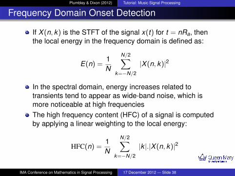
Frequency Domain Onset Detection

If X (n, k) is the STFT of the signal x(t) for t = nRa, thenthe local energy in the frequency domain is defined as:

E(n) =1N

N/2∑k=−N/2

|X (n, k)|2

In the spectral domain, energy increases related totransients tend to appear as wide-band noise, which ismore noticeable at high frequenciesThe high frequency content (HFC) of a signal is computedby applying a linear weighting to the local energy:

HFC(n) =1N

N/2∑k=−N/2

|k |.|X (n, k)|2



Frequency Domain Onset Detection

Changes in the spectrum are better indicators of onsetsthan instantaneous measures such as HFCFor example, the spectral flux (SF) onset detection functionis given by:

SF(n) =

N2−1∑

k=−N2

H(|X (n, k)| − |X (n − 1, k)|)

where H(x) is the half-wave rectifier:

H(x) =x + |x |

2

so that only the increases in energy are taken into accountAn alternative version squares the summands



Phase-Based Onset Detection

An alternative is to use phase informationIf X (n, k) = |X (n, k)| e jφ(n,k), then the phase deviationonset detection function PD is given by the mean absolutephase deviation:

PD(n) =1N

N2−1∑

k=−N2

|princarg(φ′′(n, k))|

PD(n) =1N

N2−1∑

k=−N2

|princarg(φ(n, k)−2φ(n−1, k)+φ(n−2, k))|

The PD function is sensitive to noise: frequency binscontaining low energy are weighted equally with binscontaining high energy, but bins containing low-level noisehave random phase



Phase-Based Onset Detection



Complex Domain Onset Detection

Another alternative approach is to consider the STFT binvalues as vectors in the complex domainIn the steady-state, the magnitude of bin k at time n isequal to its magnitude at time (n − 1)Also, the phase is the sum of the phase at (n − 1) and therate of phase change φ′ at (n − 1)Thus the target value is:

XT (n, k) = |X (n − 1, k)| e j(φ(n−1,k)+φ′(n−1,k))



Complex Domain Onset Detection

Sum of absolute deviations of observed values from thetarget values:

CD(n) =

N2−1∑

k=−N2

|X (n, k)− XT (n, k)|

To distinguish between onsets and offsets, the sum can berestricted to bins with increasing magnitude:

RCD(n) =

N2−1∑

k=−N2

|X (n, k)− XT (n, k)|,

if |X (n, k)| ≥ |X (n − 1, k)|0, otherwise

Onset Detection Tutorial:Bello et al (IEEE Trans SAP, 2005)



Tempo

Tempo is the rate of a pulse (e.g. the nominal beat level)Usually expressed in beats per minute (BPM)Problems with measuring tempo:

Variations in tempo: people do not play at a constant rate,so tempo must be expressed as an average over some timewindowNot all deviations from metrical timing are tempo changesChoice of metrical level: people tap to music at differentrates; the “beat level” is ambiguous (problem fordevelopment and evaluation)Strictly speaking, tempo is a perceptual value, so it shouldbe determined empirically



Timing

Not all deviations from metrical timing are tempo changes

A

B

C

D

Nominally on-the-beat notes don’t occur on the beatdifference between notation and perception“groove”, “on top of the beat”, “behind the beat”, etc.systematic deviations (e.g. swing)expressive timingsee (Dixon et al., Music Perception, 2006)



Tempo Induction and Beat Tracking

Tempo induction is finding the tempo of a musical excerptat some (usually unspecified) metrical level

Assumes tempo is constant over the excerptBeat tracking is finding the times of each beat at somemetrical level

Usually does not assume constant tempoMany approaches have been proposed

e.g. Goto 97, Scheirer 98, Dixon 01, Klapuri 03, Davies & P.05reviewed by Gouyon and Dixon (CMJ 2005)see also MIREX evaluations (Gouyon et al., IEEE TSAP2006; McKinney et al., JNMR 2007)



Tempo Induction

The basic idea is to find periodicities in the audio dataUsually this is reduced to finding periodicities in somefeature(s) derived from the audio dataFeatures can be calculated on events:

E.g. onset time, duration, amplitude, pitch, chords,percussive instrument classTo use all of these features would require reliable onsetdetection, offset detection, polyphonic transcription,instrument recognition, etcNot all information is necessary:

Original ⇒ OnsetsFeatures can be calculated on frames (5–20ms):

Lower abstraction level models perception betterE.g. energy, energy in various frequency bands, energyvariations, onset detection features, spectral features



Periodicity Functions

A periodicity function is a continuous function representingthe strength of each periodicity (or tempo)Calculated from feature list(s)Many methods exist, such as autocorrelation, combfilterbanks, IOI histograms, Fourier transform, periodicitytransform, tempogram, beat histogram, fluctuation patternsAssumes tempo is constantDiverse pre- and post-processing:

scaling with tempo preference distributionusing aspects of metrical hierarchy (e.g. favouringrationally-related periodicities)emphasising most recent samples (e.g. sliding window) foron-line analysis



Example 1: Autocorrelation

Most commonly usedMeasures feature list x(n) self-similarity vs time lag τ :

r(τ) =N−τ−1∑

n=0

x(n)x(n + τ) ∀τ ∈ {0 · · ·U}

where N is the number of samples, U the upper limit of lag,and N − τ is the integration time



Autocorrelation

ACF using normalised variation in low frequency energy asthe feature:

0 1 2 3 4 50

0.2

0.4

0.6

0.8

1

Autocorrelation Lag (seconds)

Tempo

Variants of the ACF:Narrowed ACF (Brown 1989)“Phase-Preserving” Narrowed ACF (Vercoe 1997)Sum or correlation over similarity matrix (Foote 2001)Autocorrelation Phase Matrix (Eck 2006)



Example 2: Comb Filterbank

Bank of resonators, each tuned to one tempoOutput of a comb filter with delay τ :

yτ (t) = ατyτ (t − τ) + (1− ατ )x(t)

where ατ is the gain, ατ = 0.5τ/t0 , and t0 is the half-timeStrength of periodicity is given by the instantaneous energyin each comb filter, normalised and integrated over time

0.5 1 1.5 2 2.5 30

0.1

0.2

0.3

0.4

0.5

0.6

0.7

0.8

0.9

1

Filter Delay (seconds)

Tempo



Beat Tracking

Complementary process to tempo inductionFit a grid to the events (respectively features)

basic assumption: co-occurence of events and beatse.g. by correlation with a pulse train

Constant tempo and metrical timing are not assumedthe “grid” must be flexibleshort term deviations from periodicitymoderate changes in tempo

Reconciliation of predictions and observationsBalance:

reactiveness (responsiveness to change)inertia (stability, importance attached to past context)



Beat Tracking Approaches

Top down and bottom up approachesOn-line and off-line approachesHigh-level (style-specific) knowledge vs generalityRule-based methodsOscillatorsMultiple hypotheses / agentsFilter-bankRepeated inductionDynamical systemsBayesian statisticsParticle filtering



Example: Comb Filterbank

Schierer 1998Causal analysisAudio is split into 6 octave-wide frequency bands, low-passfiltered, differentiated and half-wave rectifiedEach band is passed through a comb filterbank (150 filtersfrom 60–180 BPM)Filter outputs are summed across bandsFilter with maximum output corresponds to tempoFilter states are examined to determine phase (beat times)Tempo evolution determined by change of maximal filterProblem with continuity when tempo changes



Example: BeatRoot

Dixon, JNMR 2001, 2007Analysis of expression in musical performanceAutomate processing of large-scale data setsTempo and beat times are estimated automaticallyAnnotation of audio data with beat times at variousmetrical levelsInteractive correction of errors with graphical user interface



BeatRoot Architecture

Audio Input

Onset Detection

Tempo Induction Subsystem

IOI Clustering

Cluster Grouping

Beat Tracking Subsystem

Beat Tracking Agents

Agent Selection

Beat Track



Onset Detection

Fast time domain onset detection (2001)Surfboard method (Schloss ’85)Peaks in slope of amplitude envelope

0 0.5 1 1.5 2−0.04

−0.03

−0.02

−0.01

0

0.01

0.02

0.03

0.04

Time (s)

Am

plit

ud

e

Onset detection with spectral flux (2006)



Tempo Induction

Clustering of inter-onset intervalsReinforcement and competition between clusters

Time

Onsets

IOIs

A B C D E

C1 C1 C2 C1

C2

C3

C3

C4

C4

C5



Beat Tracking: Agent Architecture

Estimate beat times (phase) based ontempo (rate) hypothesesState: current beat rate and timeHistory: previous beat timesEvaluation: regularity, continuity & salience of on–beatevents

TimeOnsets

A B C D E F

Agent1

Agent2

Agent2a

Agent3



Results

Tested on pop, soul, country, jazz, ...

Only using onsets: ⇒Results: ranged from 77% to 100%

Tested on classical piano (Mozart sonatas, MIDI data)Agents guided by event salience calculated from duration,dynamics and pitchResults: 75% without salience; 91% with salience



Rhythm Transformation

Extend Beat Tracking to Bar level: Rhythm TrackingRhythm Tracking on model (top) and original (bottom)Time-scale segments of original to rhythm of model

Original: Model: Result:



Live Beat Tracking



Live Beat Tracking System: B-Keeper

Robertson & P. (2008, 2012)

[Video: http://www.youtube.com/watch?v=iyU61cG-j0Y]


http://www.youtube.com/watch?v=iyU61cG-j0Y


Conclusions



Conclusions

Introduction and Music fundamentalsPitch estimation and Music Transcription

Pitch Tracking: AutocorrelationNonnegative Matrix Factorization (NMF)Chord Analysis

Temporal analysisOnset DetectionBeat TrackingRhythm Analysis

Many other tasks & methods not covered here:Music audio coding, Phase vocoder, Sound synthesis, ...



Further Reading ...

Sound to Sense – Sense to Sound: A state of the art in Soundand Music Computing, ed. P Polotti, D Rocchesso (Logos, 2008)Available at http://smcnetwork.org/node/884 (PDF)

DAFX - Digital Audio Effects, ed. U Zölzer (Wiley, 2002)

The Computer Music Tutorial, C Roads (MIT Press, 1996)

The Csound Book: Perspectives in Software Synthesis, SoundDesign, Signal Processing and Programming, ed. R Boulanger

Signal Processing Methods for Music Transcription, ed. AKlapuri and M Davy (Springer 2006)

Musical Signal Processing, ed. C Roads, S Pope, A Piccialli andG de Poli (Swets and Zeitlinger 1997)

Elements of Computer Music, F R Moore (Prentice Hall 1990)

The Science of Musical Sounds, J Sundberg (Academic Press1991)


http://smcnetwork.org/node/884

Documents

Tutorial: Music Signal Processing - EECSmarkp/2012/PlumbleyDixon12-ima... · Plumbley & Dixon (2012) Tutorial: Music Signal Processing Pitch and Melody Pitch: the perceived (fundamental)