TUTORIAL IN BIOSTATISTICS: USING THE GENERAL LINEAR …

STATISTICS IN MEDICINE, VOL. 16, 2349—2380 (1997)

TUTORIAL IN BIOSTATISTICS

USING THE GENERAL LINEAR MIXED MODEL TOANALYSE UNBALANCED REPEATED MEASURES AND

LONGITUDINAL DATA

AVITAL CNAAN!*, NAN M. LAIRD" AND PETER SLASOR"

!Division of Biostatistics, Department of Pediatrics, University of Pennsylvania School of Medicine, Philadelphia,Pennsylvania, U.S.A.

"Department of Biostatistics, Harvard School of Public Health, Boston, Massachusetts, U.S.A.

SUMMARY

The general linear mixed model provides a useful approach for analysing a wide variety of data structureswhich practising statisticians often encounter. Two such data structures which can be problematic to analyseare unbalanced repeated measures data and longitudinal data. Owing to recent advances in methods andsoftware, the mixed model analysis is now readily available to data analysts. The model is similar in manyrespects to ordinary multiple regression, but because it allows correlation between the observations, itrequires additional work to specify models and to assess goodness-of-fit. The extra complexity involved iscompensated for by the additional flexibility it provides in model fitting. The purpose of this tutorial is toprovide readers with a sufficient introduction to the theory to understand the method and a more extensivediscussion of model fitting and checking in order to provide guidelines for its use. We provide two detailedcase studies, one a clinical trial with repeated measures and dropouts, and one an epidemiological surveywith longitudinal follow-up. ! 1997 by John Wiley & Sons, Ltd.

Statist. Med., 16, 2349—2380 (1997)No. of Figures: 6 No. of Tables: 8 No. of References: 34

1. INTRODUCTION

This tutorial deals with the use of the general linear mixed model for the regression analysis ofcorrelated data. The correlation arises because subjects may contribute multiple responses to thedata set. The model assumes a continuous outcome variable which is linearly related to a set ofexplanatory variables; it expands on the ordinary linear regression model by allowing one toincorporate lack of independence between observations and to model more than one error term.The types of data that can be analysed using the general linear mixed model include longitudinal

*Correspondence to: Avital Cnaan, Division of Biostatistics, Department of Pediatrics, University of PennsylvaniaSchool of Medicine, Philadelphia, Pennsylvania, U.S.A.

Contract grant sponsor: National Institutes of HealthContract grant number: GM 29745, RR00240-31

CCC 0277—6715/97/202349—32$17.50! 1997 by John Wiley & Sons, Ltd.

data, repeated measures data (including cross-over studies), growth and dose—response curvedata, clustered (or nested) data, multivariate data and correlated data. Despite this wide applica-bility, the results of such analyses are only now beginning to appear in the research literature; wewill describe briefly several recent applications. The model’s limited use is due in part to the factthat commercial software has been limited in the past, and in part to a lack of familiarity with themodel by the general statistical and medical community. The goal of this tutorial is to introducethe model and its analysis to applied statisticians, to provide some guidelines on model fitting,and to illustrate its use with two data sets. Two recent books which cover aspects of the modeland its analysis in more detail are those of Longford! and Diggle et al."

We use the term longitudinal data to imply that each subject is measured repeatedly on thesame outcome at several points in time. The main interest is usually in characterizing the way theoutcome changes over time, and the predictors of that change. A typical example of a longitudinalstudy is the Tucson Epidemiological Study of Airways Obstructive Disease, in which the effects ofsmoking onset and cessation on changes in pulmonary function were assessed.# This studyfollowed 288 subjects for 17 years. Using a random-effects model, the authors showed that thelargest beneficial effect related to quitting smoking was in younger subjects and the effectdecreased linearly with age at quitting. The advantage of this study over many studies in this areais that the modelling enabled the authors to account for both the age at onset of smoking and atquitting, in addition to other important covariates, and thus give a more comprehensive picturethan previous studies which approached only one aspect or another of the problem.

A widely used and general term is repeated measures data, which refers to data on subjectsmeasured repeatedly either under different conditions, or at different times, or both. An exampleis a study of stress and immune response in mothers of very low birth weight infants and mothersof normal weight infants.$ The two groups of mothers, comparable in sociodemographic vari-ables, were measured for stress and various immune function markers at delivery of the infant,one, two and four months post-delivery. The data for each outcome were analysed separatelyusing the balanced and complete repeated measures data approach with an unstructuredcovariance matrix for the four measurements. The mothers of the very low birth weight infantshad increased anxiety and decreased lymphocyte proliferation as well as decreased percentages ofsome immunologic cell subsets. Longitudinal models of these markers as either a linear ora quadratic function of time showed that resolution of the immunosuppression of pregnancy wassubstantially faster in mothers of very low birth weight infants than in mothers of normal weightinfants, although neither group reached normal levels by four months. The advantage of usinglongitudinal models in this study was that the time of actual measurement of the immune markerswas used, which often deviated for these mothers from the original preset schedule. This enabledthe authors to obtain a well-fitting function of time, and model the resolution of immune markers’levels.

In growth and dose—response curve data, the subjects are ordinarily measured repeatedly ata common set of ages or doses. In a study conducted in Pittsburg, the purpose was to identify theeffect of prenatal alcohol exposure on growth.% It has previously been established that prenatalalcohol exposure is associated with smaller birth size. However, it has not been clear whetherthere is subsequent catch-up growth, and cross-sectional studies have not been able to satisfactor-ily answer this question. This study followed the infants from birth to three years, and, usinga growth curve model, was able to ascertain that there was no long-term catch-up growth; thesmaller size observed at birth is maintained. The model used for analysis was a generalunbalanced repeated measures model with a fully parameterized covariance matrix.

2350 A. CNAAN, N. M. LAIRD AND P. SLASOR

Statist. Med., 16, 2349—2380 (1997) ! 1997 by John Wiley & Sons, Ltd.

Clustered data arise commonly in surveys and observational studies of populations which havea natural hierarchical structure, such as individuals clustered in households and patients clusteredin hospitals or other service delivery systems. Here interest may centre on which characteristics ofthe individual or of the cluster, or both, affect the outcome. An example of a data set wheremixed-effects models were used in a cluster setting involves a study for predicting microbialinteractions in the vaginal ecosystem.& The data for the study consisted of bacteria concentrationsfrom in vivo samples; samples could be obtained from a subject once or multiple times duringa study. The explanatory variables were concentrations of various specific bacteria, timing inmenstrual cycle, and flow stage. The general approach for inclusion of variables was a backwardelimination process. The mixed-effects modelling enabled the researchers to use all the dataavailable, account for repeats within subjects, and model total aerobic bacteria, total anaerobicbacteria and mean pH values, as three different mixed-effects models, with different fixed andrandom effects.

Multivariate data refers to the case where the same subject is measured on more than oneoutcome variable. In this setting, one is looking at the effects of covariates on several differentoutcomes simultaneously. Using the general linear mixed model analysis allows one moreflexibility than using traditional multivariate regression analysis because it permits one to specifydifferent sets of predictors for each response, it permits shared parameters for different outcomeswhen covariates are the same, and it allows subjects who are missing some outcomes to beincluded in the analysis. A study with multivariate outcomes looked at individual pain trends inchildren following bone marrow transplantation.' Children aged 6—16 years and their parentswere both asked to evaluate the child’s pain on a standardized analogue scale daily for 20 days.Empirical Bayes’ methodology was used to model pain as a quadratic function of number of dayspost-transplant. Separate models were used for describing children’s and parent’s pain ratingsand curves were compared informally. Using a single analysis with a multivariate response of thechildren and parents would have allowed a direct statistical comparison of the pain curves. Theanalysis did show that the empirical Bayes’ approach to the modelling gave a better fit thanordinary least squares (OLS) modelling separately for each child, which was possible in thisexample due to the large number of observations per child. In general, parents reported higherpain levels than the children, and there was some variability in reporting within the children byage group.

Correlated data is a generic term which includes all of the foregoing types of data as specialcases. The only restriction is that the correlation matrix of the entire data matrix must be blockdiagonal, thus the model does not accommodate time series data, in which a non-zero correlationis assumed at least between every two consecutive observations. In all of these cases theobservations are clustered, or grouped within subject. Thus we can structure the data by firstidentifying the subject or cluster, and then the repeated observation on the subject or the cluster.In describing this hierarchical structure, one might encounter in the literature the terms level oneand level two, stage one and stage two, observation level and subject level, or subject level andcluster level; the latter two are especially confusing since sometimes subject is level one andsometimes it is level two, depending upon the application. Rather than exclusively using a singleterminology in this paper, we will use the terminology most appropriate to the context andindicate in parenthesis what is meant, if necessary. In the absence of a particular context we willgenerally use subject and observation to denote the two levels of the hierarchy.

A wide variety of names are also used in the statistical literature to describe versions of thesame model, reflecting the diversity of its use in many fields. These names include: mixed linear

USING THE GENERAL LINEAR MIXED MODEL 2351

! 1997 by John Wiley & Sons, Ltd. Statist. Med., 16, 2349—2380 (1997)

model;( two-stage random effects model;) multilevel linear model;!* hierarchical linear model;!!empirical Bayes’ model,!" and random regression coefficients.!# The hierarchical structure for thedata leads naturally to the terms hierarchical linear model or multilevel linear model. Strictlyspeaking, both of these terms are used to describe models which may include more than twolevels. Examples of more than two levels are commonly encountered in the educational literaturewhere we have students grouped in classes and classes grouped in schools. Since many of thebiomedical applications deal with only two levels, we will not consider the higher level models inthis paper.

One can broadly characterize many versions of the models as methods for handling thebetween- and within-subject variability in the data. There are basically two ways which arecommonly used to model these two types of variability. The approach that seems most natural tomany investigators is to develop the model in two stages. At the first stage, we specify a separatelinear regression for the observations on each subject, as a function of covariates made on theobservations, for example, time of the observation. There will be as many of these regressions aswe have subjects; each regression must use the same set of predictor variables, so that eachregression has the same vector of coefficients, but the regression coefficients themselves areallowed to vary over subjects. At the second stage, the regression coefficients modelled at stageone are the random outcome variables, hence the terms random coefficient regressions andrandom effects models. The term mixed effects comes from combining the two regressions intoa single equation with two types of regression coefficients. The two-stage approach is attractive tomany investigators, since the subjects are explicitly treated as the unit of analysis at stage two, andone models directly the two types of regressions: the within at stage one and the between at stagetwo.

However, the approach can be limiting in the way models are developed for both the mean andthe variance-covariance structure. The mixed model approach is to simply write out a singleregression model for each observation. The model has the usual linear regression predictor for themean response, but has two types of random error terms: between-subject errors and within-subject errors. All of the observations on the same subject will have the same between-subjecterrors; their within-subject errors will differ, and can be correlated within a subject. Both within-and between-subject errors are assumed independent from subject to subject, thus observationson different subjects are independent.

In Section 2 we introduce two case studies. In Section 3 we will introduce notation, and showhow these two approaches to formulating the model are related. We then address estimation andtesting issues and offer suggestions about strategies for model specification and checking. InSection 4 we discuss statistical software and illustrate the techniques applied to the case studies inSection 5. Source code for the software programs is provided in the Appendix.

2. DESCRIPTION OF CASE STUDIES

2.1. Clinical trial in patients with Schizophrenia

As an example to motivate this tutorial, we consider a clinical trial of a medication for thetreatment of schizophrenia during an acute phase of illness.!$ This clinical trial was a double-blinded study with randomization among four treatments: three doses (low, medium and high) ofan experimental drug and a control drug with known antipsychotic effects as well as knownside-effects. Initial studies prior to this double-blinded study suggested that the experimental drug



Figure 1. Distribution of BPRS by centre for the schizophrenia trial. In this box and whisker plot the box gives theinterquartile range and the median. The whiskers are three halved the interquartile range rolled back to where there aredata. Values beyond these are plotted as outliers. The width of the box is proportional to the number of subjects observed

at baseline.

had equivalent antipsychotic activity, with lesser side-effects. The primary objectives of this studywas the determination of a dose—response relationship for efficacy, tolerability and safely, and thecomparison to the control drug. The study was conducted at 13 clinical centres, and a total of 245patients were enrolled. The primary efficacy parameter was the Brief Psychiatric Rating Scale(BPRS).!% This scale measures the extent of a total of 18 observed behaviours, reported beha-viours, moods and feelings, and rates each one on a seven-point scale, with a higher scorereflecting a worse evaluation. The total BPRS score is the sum of the scores on the 18 items. Studyentry criteria included, among others, a score of at least 20 on initial evaluation. The distributionof BPRS scores at baseline was different in the different centres, as is shown in Figure 1. The widthof the boxes is proportional to the number of patients contributing to the box, showing thedifferent sample sizes in the different centres. Analysis of variance on the baseline BPRS showsa significant difference between centres (p(0·0001). In fact, 36 per cent of the baseline variabilityin BPRS scores is explained by centre. There were no differences in baseline BPRS scores betweentreatment groups. Because of the differences at baseline between the centres and becausethe randomization was done by blocks within centre, all analyses will include centre in themodel.

Patients were evaluated at baseline and after one, two, three, four and six weeks of treatment.Patients were admitted to the hospital for the first four weeks of treatment, and discharged as theclinical condition permitted for the final two weeks. Since each patient had a different baselinevalue (range 20—69), the focus of this analysis is on the rate of change during the six weeks, ratherthan on a target desirable BPRS value. Of the patients, 134 (55%) completed the study, and 11additional patients had a week six evaluation, even though they were technically considerednon-completers. Figure 2 gives the box plots of BPRS values for each of the four treatments ateach of the observation points. The width of the box plots gives a feel for the dropout rate.

The primary reason for discontinuation was a perceived lack of effectiveness of the treatmentby the physician; there were also several withdrawals due to side-effects. Table I gives the number



Figure 2. Distribution of BPRS by treatment group at each measurement occasion for the schizophrenia trial

Table I. Schizophrenia case study: number of patients measured at each time point

Week Exp-low Exp-medium Exp-high Control Total

0 61 61 60 63 2451 55 57 57 60 2292 45 53 50 57 2053 38 46 46 51 1814 32 43 40 44 1596 29 42 36 38 145

of patients at each observation point on each treatment. Table II gives the reasons for discontinu-ation by treatment. Table I shows that the largest dropout occurred on the experimental low-dosetreatment, and Table II shows that the primary reason for this loss was perceived lack oftherapeutic effectiveness. However, the tables also show that there was substantial dropout due toside-effects in the control treatment. When a discontinuation or a dropout occurred, everyattempt was made to conduct a final observation at that time, often between two scheduled



Table II. Schizophrenia case study: reasons for discontinuation from clinical trial

Reason Exp-low Exp-medium Exp-high Control Total

Completed* 27 40 33 34 134Adverse experience 2 1 2 12 17Lack of effect 21 7 13 11 52Other reasons 11 13 12 6 42

* Several patients discontinued between weeks 4 and 6 and had a final observation, which was recorded as a week6 observation, with the appropriate non-completer coding

observation points. For purposes of this analysis, the final observation was assumed to be at thenext observation point, since the exact times were not available to us. Thus, for a patient whodiscontinued after the week 4 observation, their final observation was recorded at the week6 observation point. Therefore, there are more patients with week 6 data (Table I) than there arecompleters (Table II).

In order to further understand the dropout, Cox regression models were applied to time untildiscontinuation. In these models, discontinuation was considered a failure event, and subjectswho completed the study were considered censored at six weeks. High BPRS scores either atbaseline, or later, or large differences (increases) in BPRS scores, were all associated with a shortertime to discontinuation. However, discontinuation was not related to treatment directly (in thepresence of BPRS score), nor, in general, to centre. Results were similar either when the failureevent was defined as discontinuation of any kind or when it was defined only as discontinuationdue to lack of therapeutic response. The hazard ratio for all causes of discontinuation based ona difference of ten points on the BPRS scale was estimated as 2·4; for discontinuation due to lackof effect, the corresponding hazard ratio is 3·9.

2.2. Epidemiologic study of pulmonary function development in children

The Six Cities Study of Air Pollution and Health was designed to characterize pulmonaryfunction growth between the ages of six and eighteen and the factors that affect growth.!&A cohort of 13,379 children born in or after 1967 was enrolled in six communities: Watertown,MA; Kingston and Hariman, TN; a section of St. Louis, MO; Steubenville, OH; Portage, WI; andTopeka, KN. Most children were enrolled in the first or second grade and participants were seenannually until high school graduation or less to follow-up. At each examination, spirometry wasperformed and FEV

!, the volume of air exhaled by force in the first second, was measured. For the

purpose of the analyses demonstrated here, a subset of 300 girls from Topeka, KN, with a total of1994 measurements is presented. The data included their FEV

!, age and height. Baseline mean

age was 8.29 years (SD 1·38) and mean height was 1·29 metres (SD 0·095). The number ofmeasurements (observations) for each girl ranged from 1 to 12, and the total follow-up durationfor each girl ranged from zero to 11 years.

In our analysis, we will replicate the modelling approach suggested by Hopper et al.!' ina similar Australian study. In that study, the natural logarithm of the FEV

!was found to be well

predicted by both current height and age. despite the strong correlation between the two. He alsofound that an autocorrelation structure represented the correlation in the data better thana random effects structure.



3. THE DEVELOPMENT OF THE GENERAL LINEAR MIXED MODEL

3.1. Design considerations

We will let i"1,2, N index the subjects in the study and y!denote the vector of observations

made on the ith subject. Since subjects are allowed to have unequal numbers of observations, thevectors y

!may have different dimensions. In designed experiments, the number of observations is

usually fixed to be the same for all subjects, and inequalities arise as a result of missing data. In theschizophrenia trial (Section 2.1), the length of y

!varies from one to six depending upon if and

when the patient dropped out. In clustered data applications, where the second level might bea hospital, and observations are made on different patients within the hospital, the dimension ofy!can vary arbitrarily from hospital to hospital. We will denote the dimension of y

!by n

!, so that

the total number of observations that we have in the data set are !"!+!

n!.

Each subject also has a vector of covariates; in the schizophrenia trial (Section 2.1), the subjectlevel covariates are treatment group and centre. In addition, each observation typically has itsown covariates. The subject level covariates remain constant for all the repeated observations ona subject, whereas observation level covariates may vary as the repeated observations are made.In the schizophrenia trial, time and functions of time such as time squared etc., are the mainobservation level covariates. With clustered data where observations on different subjects are therepeated measures, the observation level covariates can be numerous, for example, age, sex,severity score, etc. In cross-over trials where one subject receives several treatments in differentperiods, both period and treatment are observation level covariates.

Many longitudinal studies where an individual is the subject typically have time as the onlyobservation level covariate. The FEV

!data example (Section 2.2) we present is an exception,

where two important predictors, age and height, are characteristics of the observation. Sometimesa variable can appear as a covariate at both levels. For example, Wechsler et al. used a two-stagecluster survey to study drinking behaviour in college students.!( First a random sample ofcolleges was drawn, then a random sample of students were surveyed in each college appearing inthe stage one sample. In the analysis, both the sex of the individual student (observation level) andthe per cent of students in the college who were a specific sex (cluster level) were used ascovariates. Another example arises in longitudinal studies where subjects are measured atdifferent initial ages, and both current age and initial age can appear as predictors in the model.!)In this case, the initial age is a subject level covariate and current age is a covariate at theobservation level.

This distinction between observational level and subject level covariates is important, since thistypically drives model formulation and selection, and determines to some extent the amount ofinformation available in the data to estimate the effects of different variables. The repeatedobservations on a subject are usually assumed to be positively correlated; this implies that theeffects of within-subject (or observation level) variables will typically be estimated with greaterprecision than the effects of between-subject variables. This is because the former are estimatedusing within-subject contrasts, and the variance of a contrast is reduced when the observationsare positively correlated. This is the basic principle of a split-plot design, where the whole plot (orbetween-subject) factor is estimated with less precision than the subplot (or within-subject) factorand the interaction of the two factors."* Likewise, the cross-over design has potential for greaterefficiency than the ‘parallel’ design because treatment contrasts are constructed using positivelycorrelated responses."! In the context of longitudinal studies, the implication is that time trends,and the effects of subject level variables on time trends, will be the effects best estimated.""



In classically designed experiments with balanced and complete data, covariates (or factors)typically vary either within subjects (observation level) or between subjects (subject level) but notboth. For example, if each schizophrenia patient (Section 2.1) were observed on all six occasions,time would vary within but not between patients, since each patient would have the same vectorof values for time. Treatment and centre vary between but not within subjects. This cleanseparation of between- and within-subject variables is a hallmark of designed experiments andhas the advantage of leading to orthogonal designs and a simplified repeated measures analysis.With observational studies, unbalanced designs and/or missing data, it is rarely possible toachieve this clear separation of between- and within-subject variables. For example, in the FEV

!data set (Section 2.2), it is not logistically possible to design the study so that each subject ismeasured at the same set of ages and heights. If a covariate varies both within and betweensubjects, it may be important to specify a model which reflects this, as in the examples previouslycited.!(,!)

3.2. Model development

We will begin in this section by formulating a two-stage or two-level model and then show itsrelationship to the general linear mixed model. Let Z

!denote the n

!!q matrix of observation level

covariates for subject i. Typically the first column is a vector of ones for the intercept, but the restof the columns must be variables that vary within the subject (observation level covariates). It isnot necessary that the values vary within every subject, that is, Z

!may be less than full rank for

some individuals, but by definition, Z!

contains the observation level covariates and shouldconsist of variables which model within-subject variation. For example, in the schizophrenia trial,we might posit that the response over time for each subject follows a quadratic curve. In this caseZ!would be n

!!3; the first column would be all ones, the second would be the time of the

observation, and the third would be time squared.Parenthetically, when modelling time trends, it is often desirable to use orthogonal poly-

nomials for numerical stability or interpretation. In doing so, it is important to use a single set oforthogonal polynomials for all subjects, even though different subjects may be observed atdifferent times. In the schizophrenia data set we could use the protocol design, that is observa-tions at weeks 0, 1, 2, 3, 4, 6 to calculate our orthogonal polynomials. Then Z

!would be

orthogonal only for the subjects observed at all six occasions, but the meaning of the coefficientsremains the same for each subject. The first-stage (or level one, observation level) regressionmodel is given by

y!#"z

!#!!#e

!#, i"1,2, N (1)

where !!represents the q!1 vector of regression coefficients for the ith subject, z

!#is the jth row of

Z!, and the e

!#are zero mean error terms. The !

!represent inherent characteristics of the subjects,

for example, parameters of a subject’s ‘true’ growth curve, and the e!#

can be thought of assampling error, or random perturbations. The e

!#are typically taken to be independently and

identically distributed with variance "". In cases where the observations have a clear ordering orstructure, some investigators alternatively assume that correlation among the e

!#is non-zero, and

varies in a systematic way. For example, with equally spaced points in time, one might assumesimple autoregressive structure (AR1) for var(e

!), where e-

!"(e

!!,2, e

!$!). When the e

!can be

thought of as measurement or sampling error the assumption of independence is natural. We letR!"var(e

!). In the second-stage regression (or level two, subject level), the !

!are regarded as



N independent q-dimensional random vectors, hence the term random regression coefficients.Their mean depends upon subject level characteristics. Let a

%!denote the vector of subject level

characteristics which affect the mean of the kth coefficient. To model the level two regression, weassume the !

!are independently distributed with

E (!!)"A

!" (2)

where

A!"

a-!!

0 2 0

0 a-"!

#0 . 2 a-

&!

"-"("-!,2 , "-

&).

and the "%’s are regression parameter vectors, of varying length depending upon the number of

subject level covariates (in a!%) which affect the mean of the kth coefficient. We further assume

var (!!)"D.

The diagonal elements of D (a q!q matrix) tell us how much the individual regression coefficients,the !

!, vary from subject to subject, after adjusting for the covariates in A

!. Thus the D matrix

models the between-subject variance, while the "" from level one models the within-subject(observation level) variance.

Because we have specified a linear model for the mean of !!, it is convenient to write !

!as

!!"A

!"#b

!

where A!" are as defined above, and the b

!are independent and identically distributed with zero

mean and variance D. Here each b!can be regarded as the ith subject’s random deviation from the

mean (A!"). Rewriting equation (1) in vector and matrix notation we have

y!"Z

!!!#e

!

which in turns implies

y!"Z

!A!"#Z

!b!#e

!. (3)

As a result

E(y!)"Z

!A

!"

and

var (y!)"Z

!DZ-

!#R

!.

Notice that when we combine the two regressions into a single model for the response as in (3), wehave two types of regression parameters, the ", and the b

!’s (since there are N subjects there are

N different b!’s). The " parameter is often termed the fixed effect, in contrast to the b

!’s, which are

called random effects or random coefficients. The b!’s can also be viewed as error terms sine they

are random variables with zero mean.



The form of the design matrix for the fixed effects in model (3) implies that any observation levelvariables must be specified as random effects if they are to be included in the model. This can bean unattractive modelling strategy in situations where there are several observation level vari-ables or they are all indicator variables, as in cross-over designs. One way to avoid thisrequirement is to force components of D to be zero. Alternatively, the model is made much moreflexible by replacing Z

!A!by an arbitrary design matrix X

!, and writing

y!"X

!"#Z

!b!#e

!. (4)

Equation (4) defines what we call the general linear mixed model. We use the term generallinear mixed model to emphasize that X

!, Z

!and R

!can be quite general; other versions of the

model place implicit constraints on one or all of these matrices. The model has two types of errorterms: the b

!are the random subject effects and the e

!are observation level error terms. In the

general linear mixed model we assume only that the b!and e

!are independently distributed with

zero mean and variances D and R!, respectively, implying that

E(y!)"X

!"

and

var (y!)"Z

!DZ-

!#R

!.

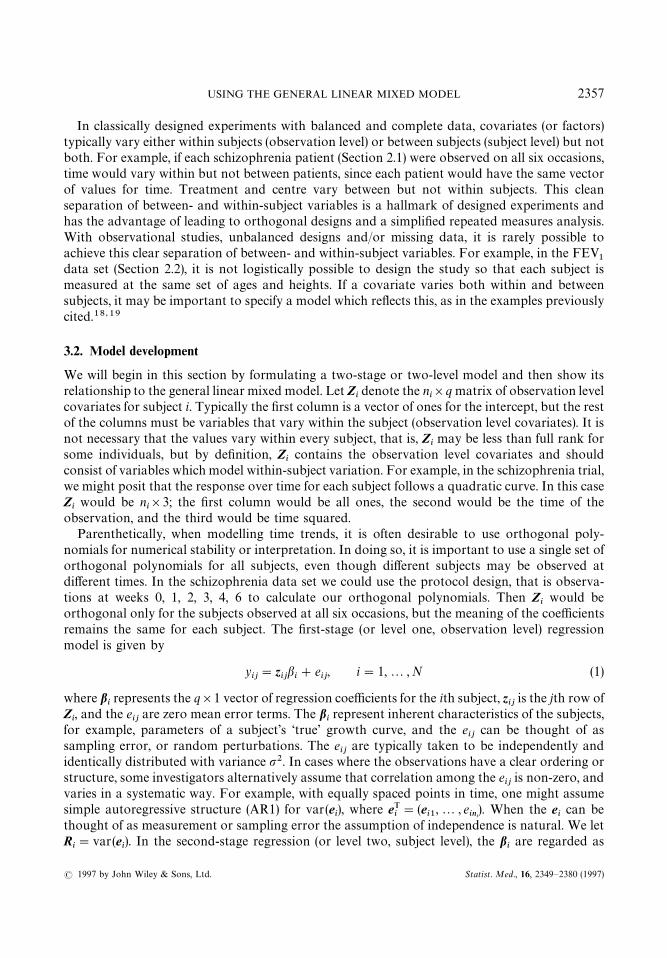
3.3. The general linear mixed model: estimation and testing

Under the assumption that the b!and e

!are independently distributed as multivariate normal,

estimation of the parameters by maximum likelihood (ML) is straightforward."# The variance-covariance parameters can also be estimated using Restricted Maximum Likelihood (REML). Asthe name implies, the REML estimates maximize the likelihood of the error contrasts, rather thanthe full data, and are often preferred over ML estimates since they yield well known method-of-moment estimators in balanced cases which have closed form solutions.

The maximum likelihood estimate of " is given by

"̂"(!X-!

VK .!!

X!)!X-

!VK .!!

y!

(5)

where

V!"var (y

!)"Z

!DZ-

!#R

!

and VK!is V

!with D and R

!replaced by their ML estimators. In practice, REML estimators are

often used to estimate V!. The estimator of " defined in equation (5) is also called the Generalized

Least Squares (GLS) estimator because it is inverse variance weighted least squares, where eachsubject’s estimated variance, V#

!, determines their weight in the estimation of ". The variance of "L is

usually estimate by

var ("̂)"(!X-!

VK .!!

X!).!. (6)

The GLS estimator (and hence the ML estimator) of " has good optimality properties that holdwithout the assumption of normality for the error terms (e

!and b

!). It is consistent, asymptotically

normal, and fully efficient if V!correctly specified the var(y

!). If we have misspecified the variance,

so that var (y!)OV

!, "̂ is still consistent and asymptotically normal, but not fully efficient, and



equation (6) is not a valid estimate of var ("̂). Liang and Zeger"$ suggest using an alternativeestimator of var("̂) which is valid when var (y

!)OV

!

var ("̂)"(! X-!

VK .!!

X!).! ! X-

!VK .!!

(y!!X

!"̂) (y

!!X

!"̂)- VK .!

!X!(! X-

!VK .!

!X!).!.

Because this estimate of var("̂) is not currently available via commercial software, we do notconsider it further. Tests for covariance structure are considered in Section 3.5.

Three approaches are used to test hypotheses of the form H*:C""0. Likelihood ratio tests can

be used with large samples, providing one uses ML, rather than REML, for model fitting.Standard Wald tests are widely available; these are also asymptotically $". Approximate F-testsfor class variables can be carried out by dividing the Wald test by the numerator degrees-of-freedom and approximating the denominator degrees-of-freedom. All of these tests are largesample, and more research on small sample adjustments is needed."% As with ordinary univariateregression, normality of the errors is not required for asymptotic normality of the estimate of ",but highly skewed error distributions can lead to invalid tests and confidence intervals, thus it iswise to consider transformations to promote normality, if appropriate.

Sometimes it is useful to have estimates of the individual random effects, the b!’s, or equiva-

lently, the !!’s. The random effects are estimated using ‘shrinkage’ or empirical Bayes estimators

which represent a compromise between estimates based only on an individual subject’s data, andestimates based only on the population mean. These estimates can be used to construct individualgrowth curves for each subject, as we illustrate with the FEV

!data (Section 2.2). For example,

Tsiatis et al."& used estimates of individual trajectories of CD4 counts to study the relationshipbetween fall in CD4 count and disease progression in AIDS. Subjects with substantial data willhave estimates close to their individual least squares curves, whereas subjects with sparse datawill have estimates close to the population mean. These shrinkage estimators are also known asbest linear unbiased predictors (BLUP)."'

3.4. Model selection

Selecting a model means specifying a design matrix for each subject, X!, the random effects (or Z

!),

and the variance-covariance structure for e!, R

!. In many cases, the mean parameters, or ", are

those of most interest and the random effects and correlation structure can be viewed as nuisancequantities. Even in this latter case it is important to model var (y

!) carefully, since it affects both

the efficiency of "̂, and the validity of the estimate of var("̂).Because E(y

!)"X

!", the mean parameters are determined entirely by the design matrix X

!; it

can include any arbitrary combination of subject level and observation level covariates that wedesire. The Z

!matrix specifies the design for the random effects. It must contain only observation

level covariates, apart from an intercept. In growth curve studies it typically contains the designon time or age. Whereas X

!determines our specification for the mean, the Z

!matrix, or

specification of random effects, only affects variance. To see this, note that it is possible to specifyno random effects so that Z

!"0. Here we still have E(y

!)"X

!" but now var (y

!)"R

!. Thus, in

many cases the use of random effects can be viewed simply as a device for modelling correlationstructure.

3.4.1. Modelling the mean

Although it is technically possible to specify X!and Z

!independently, in the case where we do

choose to include random effects, there are some guidelines one should use in choosing models. In



general, the columns of Z!should be a subset of the columns of X

!to avoid the problem of

specifying as ‘error terms’ effects which do not have zero mean. To return to our schizophreniaexample (Section 2.1), we could assume that a quadratic curve is needed to characterize the meanresponse for each subject, implying an initial large effect, followed by a levelling off of the effect.We would not want to include a quadratic effect in Z

!and omit it in the mean (X

!), since this model

would imply that each subject had a quadratic curve, but that the population curve was linear.Alternatively, omitting observation level effects from Z

!that are contained in X

!can lead to

serious underestimation of the standard errors of "̂. Consider the case where we fit linear timetrends for the mean, but assume that only the intercepts are random. In this case, Z

!is a column of

ones for each subject, and, if R!is taken to be ""I, then the variance of y

!has the compound

symmetry assumption. This assumption will cause the estimated standard errors of estimatedslopes to be too small if it fails to hold. Including the linear term as a random effect corrects thisproblem."( Assuming R

!has a richer structure is an alternative solution.

One advantage of the two-stage approach to modelling is that if X!"A

!Z!, where A

!contains

all the subject level covariates and Z!contains all of the observation level covariates, then the

Z!are necessarily a subset of X

!and any observation level variables modelled in X

!are also

contained in Z!. Recall that A

!contains the vectors of covariates, a

%!, for the regression of the kth

element of !!on subject level variables. Each of the components in !

!may have a different set of

predictor covariates. In most settings there will be considerable overlap in the covariate set, andwe may want to assume a

%!"a

!for all k.

To fix ideas, consider the schizophrenia study (Section 2.1) where we fit a quadratic responsefunction in time, so that each Z

!is n

!!3 with an intercept, a linear and a quadratic term. The

subject level characteristics are centre and treatment group. The regression model we choose forA!

will depend upon how we have parameterized time. Suppose we do not use orthogonalpolynomials so that the intercept estimates baseline (or prerandomization) means. We wouldcertainly want to include centre as a predictor of baseline means since we know that mean BPRSscores are different at baseline. This may be due to differences in centre populations or todifferences in interpreting the BPRS rating system. We could have centre as a predictor of theslope and quadratic terms as well to account for possible systematic differences in time trendsfrom centre to centre. However, if data are sparse at the centre level, we might fit a moreparsimonious model, omitting centre as a predictor of the quadratic or linear and quadraticterms. Since the study is randomized, treatment is formally not a predictor of intercept, althoughit is preferable to include it in the model, to avoid possible model misspecification. Thus we wouldinclude both centre and treatment in a

!!. If we want to test for treatment effects, we would omit

treatment as a predictor for both the linear and quadratic terms, and compare the results tomodels fit including treatment as a predictor of the linear or the linear and quadratic terms. If weuse orthogonal polynomials, then treatment effects would also have to be tested by looking at theeffect of treatment on the intercept, which now estimates a mean level over all times. Since thegroups were designed to be equivalent at baseline, testing for a treatment difference in a meanlevel which includes baseline is not very compelling. Notice that the ‘main’ effects are all specifiedby the regression of the intercept on a

!!and the remaining portions of A

!specify interactions of

subject level and observation level variables.When the observation level variables are class variables, as in cross-over and many other

repeated measures designs, using random effects beyond a random intercept is not natural, hencethe more general form of X

!is useful. In a cross-over study, one choice of X

!might be a column for

the intercept, ¹!1 columns for the ¹ treatments and P!1 columns for the P periods (or



occasions), all of which are observation level covariates. However, Z!

can still include onlya random intercept. In many longitudinal studies with a small number of observations per subjectit may also be attractive to use class variables to model the mean response over time. This allowsone to model the data without making any assumptions about time trend, rather than assuminga parametric model for how the mean response varies as a function of time. For example in theschizophrenia study, there are six possible observation times. One could use three columns ofX!for intercept, linear and quadratic terms. Alternatively, one could use five indicator variables to

uniquely define the observation times.Another issue that often arises, especially in the context of longitudinal clinical trials, is how to

handle the response made at baseline. It can be included as part of the response vector, or one canuse the baseline measurement as a subject level covariate in X

!, or one can subtract the baseline

response from each subsequent response and model the vector of changes. In the schizophreniastudy (Section 2.1), the first approach implies that each subject has six observations. The timetrend (linear or quadratic) is fit from baseline to week 6. The second approach implies that eachsubject has five observations and the intercept in the model is part of the treatment effect. Thecoefficient of the baseline covariate captures the changes in response from baseline to week 1,while the time trend coefficients capture changes from week 1 to week 6. In both approaches,because there are large differences in the response at baseline between centres, 12 indicatorvariables for the 13 centres are required in X

!for centre effects. However, in the first approach,

because the baseline is part of the response, one might need additional 12 or 24 variables forcentre by time linear or linear and quadratic interactions. In the second approach, because thebaseline in not part of the response, and the time trend coefficients model only the changes fromweek 1 to week 6, there is a potential for simpler models without centre by time interactions. Thethird approach of using changes from baseline rather than baseline as a covariate is appealing toclinicians, but is generally less statistically efficient.

3.4.2. Modelling the Variance

The variance of y!, V

!"Z

!DZ-

!#R

!, is determined by how we model R

!and the random effects.

One commonly used strategy is to set R!"""I, and use random effects to give additional

structure to V!. For example, in the schizophrenia study, setting R

!"""I implies independence

between observations within the subject. If Z!

is the n!!3 vector with intercept, linear and

quadratic time trends, then D is a 3!3 matrix which provides the additional structure to V!. This

generally works well when we are fitting parametric curves in longitudinal studies; it is especiallyuseful when subjects are observed at a large number of irregular times. A limiting feature is that ifeach subject is observed on only a few occasions, lack of identifiability and convergence problemscan occur even for only two or three random effects. This strategy is also limiting when we areusing indicator variables to model the time course, because it implies estimation of n!(n#1)/2parameters in the matrix, which may be a large number and result in poor estimation.

At the other extreme, we may assume no random effects (Z!"0), and put additional structure

on R!. If each subject has observations at the same set of ¹ occasions, and ¹ is modest relative to

N, we may choose to let R be an arbitrary ¹!¹ correlation matrix. Because R can be totallyarbitrary (positive definite) R can be called an ‘unstructured matrix’. If a subject is missing anobservation, R

!is R with the rows and columns corresponding to the missing observations

removed. In the schizophrenia study, since there are ¹"6 possible observation points andN"245, we use this approach. This strategy is also attractive for modelling multivariate data,



where each component of y!is a different variable, rather than a repeated measure on the same

variable. For example, if we wish to model height, weight and arm circumference as a function ofage and sex, the response variable has three components which are not repeats on the samevariable, and an arbitrary R may be the only logical choice for a variance structure.

Diggle") proposed a useful model which can be viewed as an extension of the general linearmixed model. He suggests using a single subject effect (b

!is scalar and Z

!a vector of ones), setting

var (e!)"""

'I, and introducing a third random error vector, say r

!, which has an autoregressive

error structure. Specifically, he assumed var (r!)"""

(, and that the correlation between r

!#and

r!%

depends only on the distance or time between the observations. He suggests several parametricforms for the correlations which model it as a decreasing function of increasing time. This modelhas the attractive feature that the variance and correlation are modelled with only a fewparameters, even when there are many different observation times, the correlation is highest formeasurements close together in time, but does not necessarily get to zero even for measurementsmade far apart. An advantage of the Diggle model is that it allows one to model correlation withvery irregularly spaced intervals using only one random effect. It does still assume constantvariance over time. In the longitudinal data setting, this assumption is often violated. Forexample, in modelling growth data, values at adolescence may show much more variability thanearly childhood data.

Specifying R!and the random effects involves a trade-off. If the number of repeated measures is

small, say less than 5, and N is substantial, say at least 100, the most attractive strategy may be toset Z

!"0 and let R

!be arbitrary. With larger numbers of repeat observations, some modelling

strategy which incorporates random effects is attractive. This is especially true for longitudinaldata which is highly unbalanced, for example, observations are made at arbitrary times leading toa highly unbalanced data set such as in data registries involving patient follow-up. In this case,setting R

!"""I and using random effects may be the only feasible strategy. The Diggle")

approach is one that has been used successfully to model FEV!

data (Section 2.2).!'It is not possible to include an arbitrary set of random effects and let R

!be completely general,

because this results in overparameterization. Consider the following simple case. If we specify thatR has compound symmetry structure and let Z

!be a vector of ones, then V

!is the sum of two

matrices with identical structure (constant variance on the diagonal and same correlation at allpositions off the diagonal) and they are not separately identifiable. With large numbers of repeatmeasures, it is possible to fit several random effects and specify some non-saturated structure forR!, such as autoregressive, but general rules for identifiability of model parameters are not

available. A simple approach that seems to work well in many situations is to either load up thevariance in the random effects and set R

!"""I, or set Z

!"0 and allow R

!to be arbitrary.

Practical experience suggests that the simple compound symmetry assumption, which involvessetting R

!"""I and using a single random subject effect (intercept), typically fails to adequately

model the variance structure. Often adding just a single additional random effect is adequate.

3.5. Model checking

Many issues of model sensitivity and checking goodness-of-fit are exactly the same as those whicharise in ordinary least squares regression. The standard residual diagnostics can be helpful; it canalso be useful to look at residuals stratified on time (in longitudinal studies) or by subject.Waternaux et al.#* suggest methods for outlier detection based on the empirical Bayes estimates of thesubject random effects. They can help identify outlying subjects, rather than outlying observations.



One issue that is different from ordinary univariate regression is that a model must be specifiedfor var(y

!). Likelihood ratio tests based on the REML likelihoods can be used informally for

comparing nested models for var (y!), but the asymptotic $" distribution fails to hold because the

null hypothesis corresponds to a boundary value. Some computer packages give goodness-of-fitmeasures based on Schwartz’s Bayesian Criterion and the Akaike’s Information Criterion. Bothof these are functions of the likelihood, with a penalty for the number of covariance parameters.For both criteria, larger values imply better fitting models, and can be used to compare non-nestedmodels. More informally, in the balanced setting, one can compare a fitted model with the empiricalcovariance matrix, which is obtained by fitting the unstructured variance model. This is preferableto using the ‘all available pairs’ estimate available from some software packages, since the latter maybe biased by missing data. Diggle") and Laird et al.!) illustrate the use of the empirical semi-variogram to check model adequacy of the correlation structure in more complex settings wheremodels are not nested; it is not currently available with software for the general linear mixed model.

3.6. Missing data

From a technical point of view, it is easy to handle missing responses in the outcome since there isno requirement that all n

!are equal, or that subjects are measured at the same set of occasions. All

that is required is that the design matrix and correlation structure can be specified for the vectorof responses that are observed. A bigger issue is the validity of the estimates in the presence ofmissing data. If the missingness is unrelated to outcome, then the ML estimates are valid and fullyefficient. This is probably the case with most missingness in the FEV

!data set (Section 2.2) since

data were collected in school, and missingness was related to school attendance, and likely not tochild FEV

!.

The probability of missingness may often be related to covariates; in principle this causes nodifficulty but in practice it implies one should take care in the process of model selection. Forexample, suppose children who smoke are likely to have poorer attendance records, or leave theschool early. If smoking affects FEV

!, then the probability of missingness is indirectly related to

outcome. In this case, smoking status should be used as a subject level covariate in the model forFEV

!in order to avoid bias due to missing data. The parameter estimates would then model

mean response conditional on smoking. If we want to estimate the marginal mean FEV!

at eachage, unconditional on smoking, we will need to take the appropriate weighted combination ofsmoker and non-smoker means.

If missingness is related to observed responses but not missing ones, termed Missing atRandom (MAR) by Little and Rubin,#! then the estimates will be valid and fully efficient providedthat the model assumed for the data distribution is correct. Dropouts in longitudinal studies aresometimes regarded as MAR if one can argue that the likelihood of dropping out only dependsupon (observed) past history, and not on future values. In the schizophrenia trial (Section 2.1),Cox regression analysis was used to show that the probability of discontinuing on protocol, andhence subsequent missingness, was strongly related to changes in BPRS. The validity of the MLanalysis that we present rests on the assumption that conditional on their observed BPRSoutcomes, treatment group and centre, the future BPRS values of a discontinued subject can bepredicted from the assumed multivariate normal distribution. The implication of this is that thedistribution of future values for a subject who drops out at time t is the same as the distribution offuture values for a subject who remains in at time t, if they have the same covariates, and the samepast history of outcome until and time t.



If dropout depends upon some other process which is related to outcome, then conditioning onpast outcomes may not capture all of the dependence of dropout on future (unobserved) outcome,and the dropout process is informative, or nonignorable. For example, in the schizophrenia trial,discontinuing on protocol might have reflected decisions based on physician assessment ofpatient condition only weakly related to BPRS. The Cox regression shows that BPRS is stronglypredictive of discontinuation, and is consistent with the assumption that the missingness is atrandom, but does not preclude a non-ignorable mechanism.

The general case of non-ignorable missingness occurs when the probability that a response ismissing is directly related to the missing outcome. For example, in trials of patients undergoingchemotherapy treatment for cancer, quality-of-life assessments may be required on a quarterlyschedule. Most quality-of-life forms are self-report and may require substantial effort on the partof the patient. Patients who are experiencing poor quality-of-life are likely to be far less able tocomplete the self-report required for response. Obtaining valid estimates of population para-meters in this setting is far more complicated, since we are in a situation of having to makeassumptions about the distribution of the missing outcomes which cannot be fully tested by thedata.

4. SOFTWARE FOR MAXIMUM LIKELIHOOD ANALYSIS OF GENERAL LINEARMIXED MODEL

Several statistical software packages are available for the analysis of correlated data. Theseinclude BMDP-5V, SAS, and ML3, among other. HLM and S-plus are other programs available,but these are restricted to analysis of random effects models, and are not discussed here.

Most of the software packages offer a choice between maximum likelihood and restrictedmaximum likelihood estimation. The optimization algorithm may be chosen as Newton—Raph-son, Fisher Scoring, or the EM algorithm. The user is required to specify an equation for meanresponse that is linear in the fixed effects, and to specify a covariance structure. The user mayselect a full parametrization of the covariance structure (unstructured) or choose from amongstructured covariances which are more parsimonious. The covariance structure is also deter-mined by inclusion of random effects and specification of their covariance structure.

Output generated includes a history of the optimization iterations, estimates of fixed effects,covariance parameters, and their standard errors. Estimates of user-specified contrasts and theirstandard errors are also printed. Graphics facilities for these software packages are currentlylimited. Parameter estimates, fitted values and residuals produced from a model run may be savedas data sets, and supplied to programs suited for graphics.

SAS PROC MIXED was designed for the analysis of mixed models. It provides a very largechoice of covariance structures. In addition to the unstructured, random effects and autoregres-sive, it can fit the Diggle model with R

!"""I#S

!, where S

!can have one of several autoregres-

sive structures. In addition, covariance can be specified to depend on a grouping variable.Separate analyses can be run on subgroups of the data through use of a single BY statement.PROC MIXED conveniently provides empirical Bayes estimates (random effects and predictedvalues). SAS constructs approximate F-tests for class variables by dividing the Wald test by thenumerator degrees-of-freedom and approximating the denominator degrees-of-freedom. Allcomponents of the SAS output, such as parameter estimates, residuals and contrast matrices, canbe saved as data sets, for purposes of graphics or manipulation by other SAS procedures. TheFEV

!data set (Section 2.2) was analysed using SAS.



BMDP-5V was designed for the analysis of unbalanced repeated measures data. It alsoprovides a large variety of options for the covariance structure, and for estimation. The dataset-up is different between SAS and BMDP. In SAS PROC MIXED, every observation withina subject constitutes a line, or a record. In BMDP5V, the line or record is the entire subject, withall its observations. This makes BMDP particularly useful and easy to manipulate when studiesare planned to be complete and balanced. It also allows one to very easily see the patterns ofmissingness. However, for epidemiological studies, which are inherently unbalanced, setting thedata up in BMDP may be awkward. The schizophrenia case study (Section 2.1) was analysedusing BMDP. BMDP provides a Wald test to examine overall effects of class variables, such asclinic, in the schizophrenia study. This is similar to the F-test provided by SAS.

Several models were run both in BMDP and SAS. Results were identical up to fourth decimalplace for the log-likelihood, regression coefficients estimates and their standard errors, andestimates of covariance parameters. Both SAS PROC MIXED and BMDP-5V, as parts of largerpackages, have the flavour of their parent packages. In both programs, in order to run a differentmodel on the same data set, one needs to enter the editor, change the model specifications andthen rerun the program. This is somewhat short of fully interactive.

ML3, which stands for Software for Three Level Analysis, was developed for applicationswithin the fields of education and human growth.#" Nutall et al.## used ML3 for modellingachievement scores in 96 schools in London, where the observations were on individual studentsand the clusters were schools. Input and manipulation of data are very similar to MINITAB,making it relatively easy to use for MINITAB users. The program is highly interactive. The usersets the model, and with a one word command sees the specifications. The user can run the model,and view, save, or print out what they want to see, and in the same session, simply change oneparameter, for example, add a fixed effect, and rerun the model. In that interactive environment,ML3 is somewhat more convenient to use than either BMDP or SAS, which require an actualseparate batch run, when the user wishes to change one thing in the model.

5. CASE STUDIES ANALYSIS

5.1. Schizophrenia clinical trial

5.1.1. Design considerations

The clinical trial in schizophrenia (Section 2.1) is a typical example of a study with a pre-plannedrepeated measures design, in which incomplete data resulted from study dropouts, necessitatingthe use of the mixed model, instead of the regular repeated measures approach. Because therewere only six different observation points, and 245 subjects, we used an unstructured covariancematrix in the analysis. In addition, we focused on the nature of the rate of change in BPRS acrosstime. The fact that there were only six different observation points enabled us to construct modelswith indicator variables for all observation points, reflecting no specific trend across time, andcompare any fitted function of time (such as a linear or quadratic time trend) with the model withindicator variables to examine goodness-of-fit.

In order to stabilize polynomial effects in the time trends, we chose a location transformationby subtracting three weeks from the week number, which makes the data for the linear andquadratic effects for subjects with complete data nearly orthogonal to each other. In a model witha linear or a linear and quadratic effect using the untransformed time scale, the estimate of the



intercept reflects an estimate of BPRS score at baseline. In a model using the suggestedtransformed time scale, the estimate of the intercept reflects the mean BPRS at three weeks. Ina linear model, the linear coefficient reflecting the linear rate of change of BPRS with time remainsthe same, regardless of transformation. In the quadratic model, however, the quadratic coefficientremains the same after the transformation, but the linear coefficient changes as a results of thetransformation.

5.1.2. Model selection and testing

Our first approach to the analysis was to use BPRS scores from all six observations as responsevariables y

!#, i indicating subject number and j indicating the observation number ( j"1,2 , 6).

We compared models with linear and quadratic time trends (observation level covariates) to themodel with indicator variables for each time point. We chose not to fit trends with time higherthan quadratic because those are difficult to interpret in this study. A combination of linear andquadratic effects can be interpreted as a decrease in BPRS scores linearly with time, and thedecrease is larger initially, and then levels off, hence the quadratic term. Plots of the data supportthis interpretation. We also added first-order interactions both between subject-level covariates(for example, treatment!centre) and between subject and observation level covariates (forexample, treatment!week). The model with a quadratic effect for time, as well as a quadraticeffect for the interaction between time and centre provided a substantially better log-likelihoodthan the model with indicators at each time point and without a time by centre interaction,although at a cost of estimating 21 more parameters. A direct log-likelihood comparison is notpossible, since these models are not nested.

There were several unattractive features in this quadratic model. The first is the time—centrequadratic-interaction. While it is not surprising that the centres had different baseline BPRSmeans (reflecting either somewhat different patient populations at the centre or somewhatdifferent interpretations of the BPRS scoring systems), it is unexpected to see a stronglysignificantly different change across time between the centres, given that all centres gave the sametreatments according to the same protocol. Moreover, a close examination of the within-subjectcorrelations from the estimated model shows stronger correlations between all observation pointsbeyond baseline than correlations with the baseline values, and a tendency of decreasingcorrelations with increasing time differences. Finally, a quadratic trend without the time—centrequadratic interaction did not provide a fit that was comparable to the model with no assumptionson the time trend. Observing also that 36 per cent of the baseline variability in BPRS is explainedby centre alone, we chose to fit subsequent models using the baseline BPRS score as a subjectlevel covariate, rather than a response.

Table III gives the BMDP results of models fitted to the data presented as five response values(weeks 1, 2, 3, 4, 6), with the baseline BPRS score as a subject level covariate. This reduced thenumber of subjects included in the model from 245 to 233, since 12 subjects had no observationsbeyond baseline, and thus no responses in these models. Adding the baseline BPRS score asa subject level covariate reduced substantially the variability to be fit by other terms in the model,suggesting that the approach to analysing the data as at most five responses rather than sixresponses was preferable. In models 1 and 2, time is entered as linear and quadratic observationlevel terms; model 2 also contains a subject level main effect of treatment. A comparison betweenmodels 1 and 2 shows that the addition of a treatment effect was not significant. The addition ofa different linear trend in time among the treatments (observation level) was also non-significant



Table III. Models for schizophrenia study. Baseline BPRS and centre are included as covariates in allmodels

Model Variables in model ML log- Number of Baseline Week Week" Test effect p-valuenumbers likelihood reg parms BPRS coefficient coefficient

coefficient

1 Week, week" !3266·33 16 0·65 !1·55 0·382 Trt., week, week" !3263·85 19 0·64 !1·56 0·38 Trt 0·213 Trt., week, week",

week!trt. !3261·90 22 0·65 !1·50 0·38 Week!trt. 0·264 Trt., week indicators!3256·29 21 0·63 — —5 Trt., week, week",

week!centre !3257·07 31 0·64 !1·72 0·38 Week!cent-re 0·25

6 Trt., week, week",status !3164·03 20 0·58 !2·35 0·48 status )0·0001

For all models, both the linear time trend coefficient (week) and the quadratic, as well as the overall centre effect, weresignificant at the 0·001 level by the Wald test. Overall treatment effect was not significant in any model

(week!treatment, model 3, compared to model 2). Since the purpose of the study was to showthat the experimental treatment was as efficacious as the active control, this result is notsurprising. The non-significance of the treatment effect does not, of course, imply equivalence.The four treatment effects need to be tested for equivalence, which is not the focus of this tutorial,and is not considered here. Model 4, which reflects no assumption on the time trend, has all thetime indicators significant. A comparison with model 2, gives a likelihood ratio test of 15·12 ontwo degrees of freedom, implying that a quadratic in time model does not adequately describe thetime trend.

5.1.3. Estimation and effect of missingness

Model 5 shows the addition of a centre by week interaction (observation level covariate). Theoverall log-likelihood is comparable to the unrestricted model 4, although with ten moreestimated parameters. The overall centre by linear week interaction was not a significant term bythe Wald test, nor was it a significant contribution beyond model 2 by a likelihood ratio test.From Table III we can see that results are very similar for models 1, 2 and 3 in terms of bothcoefficient values and log-likelihoods. The coefficient of baseline BPRS indicates a substantialdrop from baseline to week 1 in BPRS of approximately one-third, which on average meansa reduction of 12 points. Correcting for the linear and quadratic effect on that first week, addsapproximately five points, for a net effect of an estimated mean seven point drop during the firstweek of treatment. Subsequently, between weeks 1 and 6 there is a continued, slower drop whichgives a total estimated additional reduction of six points by study end. Comparing model 2 tomodel 4 shows that the quadratic model does not provide a completely adequate description ofthe time trend. Table IV gives the model fitted variance-covariance matrix for model 2. Standarddeviations are between 9.5 and 14 BPRS points.

Model 6 was examined in an effort to study the effect of dropout. The study protocol called fordiscontinuation of the study if there was a perceived lack of therapeutic effect of the study drug.The decision to discontinue a patient on those grounds was done without knowledge of treatment



Table IV. Covariance matrix for schizophrenia study. Model with baseline BPRS, treatment,centre, week, and week" (Correlations above the diagonal; covariances below)

Week 1 Week 2 Week 3 Week 4 Week 6

Week 1 92·20 0·63 0·52 0·34 0·35Week 2 66·04 120·30 0·76 0·64 0·60Week 3 64·07 106·26 161·80 0·77 0·72Week 4 43·67 91·75 127·41 169·22 0·85Week 5 46·79 93·07 128·92 155·08 196·37

Table V. Covariance matrix for schizophrenia study. Model with baseline BPRS, treatment,centre, week, week", and patient status (correlations above the diagonal; covariances below)

Week 1 Week 2 Week 3 Week 4 Week 6

Week 1 85·47 0·61 0·500·50 0·27 0·32Week 2 55·54 95·50 0·75 0·59 0·60Week 3 50·92 80·34 121·02 0·73 0·67Week 4 26·14 60·01 83·07 108·13 0·77Week 5 31·30 60·96 76·92 83·39 107·34

assignment and not based on BPRS scores. However, the final observation in the study for thosecases was performed after the decision to discontinue. Thus, we added an observation-levelindicator covariate of patient status. This variable was defined as 0 while the patient was on studyand as 1 at the last observation if the patient was discontinued due to lack of therapeutic effect, sothat the last observation reflected a status of being off-study. Model 6 provided the highestlikelihood with the fewest parameters of any of the previous models.

Table V gives the variance-covariance matrix of this model, and all variances are reduced ascompared to model 2 (SDs are 9—10.5 BPRS points in model 6), and this reduction becomes moresubstantial in later time points. Both Tables IV and V show an increase in variance with time; thisis a common phenomena in longitudinal studies. One reason is that entry to the study is restrictedto those patients with BPRS of 20 or greater, thus limiting the total range, as compared to latertime points. In model 6, both the baseline BPRS coefficient and the linear trend coefficientshowed an even greater mean reduction in BPRS than other models in Table III, which isadjusted by an increase in BPRS in those patients who were discontinued due to perceived lack oftherapeutic effect. The estimated treatment effects for this model, which includes status, can beinterpreted as effects of treatment, assuming that patients are maintained on therapy. In thatsense it might be viewed as an explanatory analysis.#$

To illustrate the relationship between the notation of the models in Section 3 and the modelspresented here, we define model 6 in the terminology of the general linear mixed model aspresented in equation (4). Recall that X

!is defined by a combination of subject level and

observation level covariates. The subject level covariates are: (i) a column of 1’s for the intercept;(ii) the subject’s baseline BPRS value; (iii) three columns of treatment indicators; (iv) 12 columns ofcentre indicators. The observation level covariates are: (a) a linear week effect (range !2 to #3;(b) a quadratic week effect (range 0 to 9); (c) a column for the status variable. The vector y

!has



Table VI. Regression coefficients and standard errors for three covariance models

Variable name Unstructures covariance Random effects Autoregressive

Estimate SE Estimate SE Estimate SE

Intercept 2·13 2·47 1·90 2·51 3·73 2·54Baseline BPRS 0·64 0·067 0·65 0·067 0·58 0·069Low dose treatment 1·93 1·04 2·04 1·06 2·69 1·10Medium dose treatment !1·86 1·02 !1·64 1·03 !1·75 1·06High dose treatment 0·10 1·03 !0·13 1·05 !0·36 1·07Week !1·56 0·25 !1·52 0·25 !1·91 0·23Week" 0·38 0·084 0·37 0·085 0·36 0·090

between one and five elements, depending on the number of observations beyond baseline.We assume, as defined earlier, that Z

!"0 and that var (y

!) is arbitrary. The BMDP code

associated with this model is given in Appendix I.If we wish to use a random effects approach. we would define Z

!to have three columns

including an intercept, slope and quadratic effect. The observation level covariate status, beingbinary, would not have an associated random effect. Examining the within-subjects model-basedcorrelations matrices in both models 2 and 6 showed similar correlations of 0·5—0·85 betweenBPRS scores at different observation points, except for between week 1 and weeks 4 and 6, whichwere approximately 0·3. In addition, there was uniformly a decreasing correlation betweenobservation points as the time gap was larger. This suggested exploring a random effects errorstructure with random intercept, linear trend and quadratic trend, that is, all observation-levelcovariates as recommended in Section 3, as well as exploring an autoregressive structure(AR1).

Table VI gives the estimated coefficients and SEs under all three covariance structures formodel 2. Investigating the coefficients shows that all three models estimate the coefficient of thebaseline value to be approximately two-thirds. The unstructured covariance matrix and therandom effects model had similar linear and quadratic time trends coefficients, indicatinga reduction of six points from week 1 to week 6 beyond the initial reduction in the first week. TheAR1 model predicted a reduction by eight points. Part of the reason may be due to themodel-estimated within-subject covariance matrices. In both the unstructured and the randomeffects models, the variances and covariances are not restricted, and, as Table IV shows for theunstructured covariance model, the variances increase with time. The AR1 model constrains thestructure to equal variances at all observation points, and covariances depend only on the timegap. Thus, this model assumes more precision than the other models for the late time points inthis study, and thus gives them relatively more weight. Because a substantial part of the dropoutis due to a perceived lack of therapeutic effect, at least theoretically, the mean of week 6 BPRSvalues may be biased down. Thus, an estimate which puts slightly more weight on week 6 willshow overall a slightly larger reduction in the BPRS score. It should be stressed that thisdifference between the AR1 model estimates and the two other models is primarily a resultof different estimated within-subject variances and not different estimated within-subjectcorrelations.

Figure 3 illustrates the fitted model 6 and the observed data for two subjects in the mediumdose treatment group.



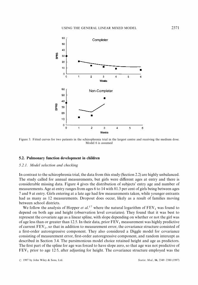
Figure 3. Fitted curves for two patients in the schizophrenia trial in the largest centre and receiving the medium dose.Model 6 is assumed

5.2. Pulmonary function development in children

5.2.1. Model selection and checking

In contrast to the schizophrenia trial, the data from this study (Section 2.2) are highly unbalanced.The study called for annual measurements, but girls were different ages at entry and there isconsiderable missing data. Figure 4 gives the distribution of subjects’ entry age and number ofmeasurements. Age at entry ranges from ages 6 to 14 with 81.3 per cent of girls being between ages7 and 9 at entry. Girls entering at a late age had few measurements taken, while younger entrantshad as many as 12 measurements. Dropout does occur, likely as a result of families movingbetween school districts.

We follow the analysis of Hopper et al.!' where the natural logarithm of FEV!

was found todepend on both age and height (observation level covariates). They found that it was best torepresent the covariate age as a linear spline, with slope depending on whether or not the girl wasof age less than or greater than 12.5. In their data, prior FEV

!measurement was highly predictive

of current FEV!, so that in addition to measurement error, the covariance structure consisted of

a first-order autoregressive component. They also considered a Diggle model for covarianceconsisting of measurement error, first-order autoregressive component, and random intercept asdescribed in Section 3.4. The parsimonious model choice retained height and age as predictors.The first part of the spline for age was forced to have slope zero, so that age was not predictive ofFEV

!prior to age 12·5, after adjusting for height. The covariance structure employed was the



Figure 4. The distribution of age at entry for the FEV!

data, showing also the number of measurements obtained on eachsubject

measurement error plus first order autoregressive. In this data set there were no subject levelcovariates except for intercept.

Previous analyses of our data suggested the use of log height rather than height as a predictorof FEV

!; we also had no reason to support the spline with knot at age 12·5 years. Thus our first

step was to fit models with both versions of height (linear and logarithmic) and varying the knotpoint for the spline from 11·5 to 17·0 in six month increments. We did not assume that the slopefor age prior to the knot was zero. We used the Diggle covariance structure, and then usedlikelihood values and residual plots to choose the best model. Residual plots revealed anobservation that was clearly outlying. This observation was of a subject who only had onemeasurement available. We dropped this observation, so that all subsequent analysis is based onthe data of 299 girls. The spline with knot at age 16 provided the highest likelihood, and thelikelihood ratio test comparing this model to the simpler model with linear age, was highlysignificant (p(0·0001). Table VII gives the likelihood values for these models.

Plots of residuals, ordered by age, are given in Figure 5. The three graphs on the left side giveresiduals for models obtained with knots at ages 15, 16 and 17, respectively. The three graphs onthe right are similar, except height has been transformed by taking the natural logarithm. It isdifficult to discern a pattern in the residuals. A lowess curve is run through the data points of eachplot. The best fitting model should have a lowess curve that is closest to a line with slope zero.Inspecting the graphs, one sees that the lowess curves are not very different. The model with knot



Table VII. Likelihood values for FEV!

data

Age at knot (2 log-likelihood)Covariate used

Height Log height

11·5 4743·68 4734·5912·0 4743·51 4730·2512·5 4741·64 4720·3213·0 4740·24 4711·0913·5 4742·97 4708·3714·0 4754·66 4719·1614·5 4772·73 4739·1415·0 4792·16 4760·6815·5 4803·19 4773·0816·0 4805·90 4775·9016·5 4795·08 4764·4617·0 4780·84 4749·42

at age 16 seems to have the flattest curve for later ages, giving further evidence that age 16 is thebest choice for the knot. The plots for the models using logarithm of height are not much differentfrom plots for models using height. We keep height (untransformed), and age as a spline with knotat age 16, in subsequent analyses.

Table VIII shows the SAS results of fitting several different models to the FEV!

data; all havethe same mean predictors (height and spline for age with knot at age 16), but the models havedifferent covariance structures. Appendix II gives the SAS code for using the Diggle model for thecovariance, and the results of this model are given in column 4 of Table VIII. The coefficient ofAGE1 gives the slope prior to age 16 and the coefficient of AGE2 gives the deviation of thepost-16 slope from the pre-16 slope. Age and height are significant predictors of FEV

!. Log FEV

!is predicted to increase by 0·034 per year prior to age, 16, and 0·014 per centimetre of growth. LogFEV

!changes with age beyond age 16 are predicted to be !0·006 per year. A model was fit

where the slope beyond age 16 was forced to be zero (not shown). The one degree-of-freedomlikelihood ratio test was not quite significant (P"0·083). This finding differs from the Hopperresult, where log FEV

!was found to have zero slope with respect to age less than 12·5, and

positive slope beyond age 12·5.The remaining columns of Table VIII show the results of fitting the same model for the mean,

but making different assumptions about the variance. Because of the highly unbalanced nature ofthe data, and the large number of potential observations of each subject, it is not possible to fit anunstructured covariance matrix. We fit the models used by Hopper, and also one which treats thetwo slopes on age as random effects. For this last model, the Z

!matrix contains an intercept,

AGE1 and AGE2. Apart from the OLS fit, the estimated regression parameters are all verysimilar, as are their estimated standard errors. The OLS fit gives quite different estimates andstandard errors, although in this case the inferences are similar. The Diggle model yields thehighest likelihood, again consistent with Hopper’s result.

Figure 6 gives empirical Bayes estimates for selected girls (broken curve), contrasted withordinary least squares estimate based on the subject’s data (solid curve). Notice that these curves



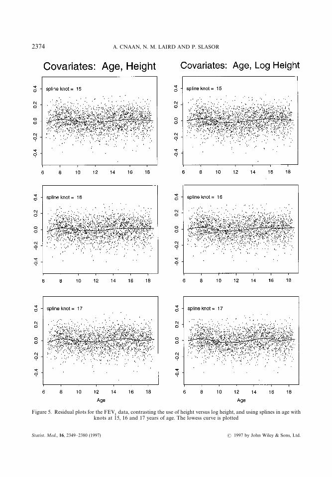
Figure 5. Residual plots for the FEV!

data, contrasting the use of height versus log height, and using splines in age withknots at 15, 16 and 17 years of age. The lowess curve is plotted



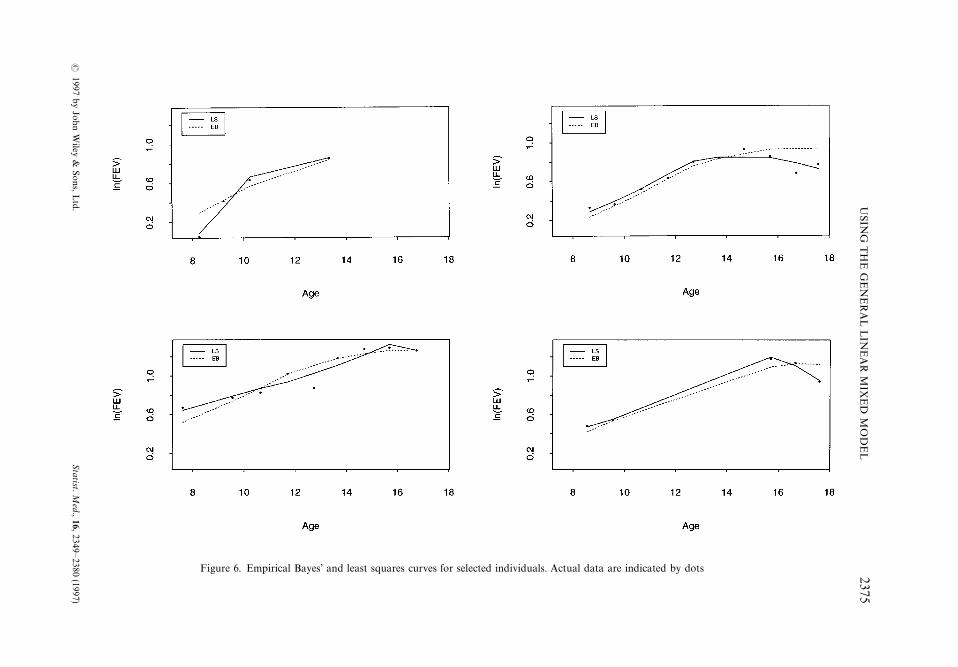
Figure 6. Empirical Bayes’ and least squares curves for selected individuals. Actual data are indicated by dots

USIN

GT

HE

GE

NE

RA

LL

INE

AR

MIX

ED

MO

DE

L2375

!1997

byJohn

Wiley

&Sons,L

td.Statist.M

ed.,16,2349—2380(1997)

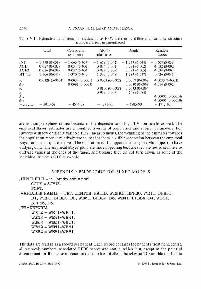
Table VIII. Estimated parameters for models fit to FEV!

data using different co-variance structure(standard errors in parentheses)

OLS Compound AR (1) Diggle Randomsymmetry plus error slopes

INT !1·778 (0·038) !1·663 (0·037) !1·679 (0·042) !1·679 (0·044) !1·708 (0·038)AGE1 0·027 (0·002) 0·034 (0·002) 0·034 (0·002) 0·034 (0·002) 0·032 (0·002)AGE2 !0·026 (0·006) !0·037 (0·004) !0·039 (0·005) !0·039 (0·005) !0·034 (0·004)HT (m) 1·506 (0·041) 1·380 (0·040) 1·390 (0·046) 1·389 (0·047) 1·426 (0·041)

""'

0·0129 (0·0004) 0·0039 (0·0001) 0·0023 (0·0002) 0·0017 (0·0003) 0·0033 (0·0001)d**

0·0092 (0·0008) 0·0080 (0·0009) 0·014 (0·002)""(

0·0106 (0·0008) 0·0033 (0·0004)% 0·953 (0·007) 0·665 (0·084)d!!

0·00007 (0·00014)d""

0·00007 (0·00018)!2log L !3010·58 !4644·38 !4791·71 !4805·90 !4742·03

are not simple splines in age because of the dependence of log FEV!

on height as well. Theempirical Bayes’ estimates are a weighted average of population and subject parameters. Forsubjects with few or highly variable FEV

!measurements, the weighing of the estimates towards

the population mean is relatively strong, so that there is visible separation between the empiricalBayes’ and least squares curves. The separation is also apparent in subjects who appear to haveoutlying data. The empirical Bayes’ plots are more appealing because they are not so sensitive tooutlying values at the ends of the range, and because they do not turn down, as some of theindividual subject’s OLS curves do.

APPENDIX I: BMDP CODE FOR MIXED MODELS

/INPUT FILE"‘c: &bmdp&schiz.por’.CODE"SCHIZ.PORT.

/VARIABLE NAMES"TRT, CENTER, PATID, WEEKO, BPRSO, WE11, BPRS1,D1, WE21, BPRS2, D2, WE31, BPRS3, D3, WE41, BPRS4, D4, WE61,BPRS6, D6.

/TRANSFORMWE12"WE11*WE11.WE22"WE21*WE21.WE32"WE31*WE31.WE42"WE41*WE41.WE62"WE61*WE61.

The data are read in as a record per patient. Each record contains the patient’s treatment, centre,all six week numbers, associated BPRS scores and status, which is 0, except at the point ofdiscontinuation. If the discontinuation is due to lack of effect, the relevant ‘D’ variable is 1. If data



are missing, for example, discontinuance after week 4, or week 2 skipped, the fields contain ‘ · ’ tosignify missing data.

/GROUP VARIABLE"TRT, CENTER.CODES (TRT)"1,2,3,4.NAMES (TRT)"‘Lo’, ‘Med’, ‘Hi’, ‘Cont’.

The categorial variables of treatment and centre are defined, so that BMDP can create theappropriate indicator variables in the model.

/DESIGN DPNAME"BPRS.DPVAR"BPRS1, BPRS2, BPRS3, BPRS4, BPRS6.REPEAT"WEEK.LEVEL"5.CVNAME"BPR0, WE1, WE2, STATUS.BPRO"BPRS0, BPRS0, BPRS0, BPRS0, BPRS0.WE1"WE11, WE21, WE31, WE41, WE61.WE2"WE12, WE22, WE32, WE42, WE62.STATUS"D1, D2, D3, D4, D6.

The definition of dependent and independent variables is made, including the complete structureof the design matrix. BPRS is identified as the dependent variable. This paragraph identifies thefact that there is a potential for five repeats within each record, and gives a name for each variable,dependent or covariate, that can have five repeats, as well as the associated data variables whichform these five repeats.

/STRUCTURE TYPE"UNSTRUC.

This command identifies the covariance structure as unstructured, thus in this case a five by fivematrix. Other options would have been: ‘TYPE"CS’ (compound symmetry), ‘TYPE"AR(1)’(first-order autoregressive), ‘TYPE"BANDED’ (banded, or general autoregressive).

Structures which would require additional input would be: ‘TYPE"RANDOM’ (randomeffects), ‘TYPE"ARANDOM (random effects with AR(1) residual correlation structure),‘TYPE"LINEAR’ (general linear structure), ‘TYPE"USER’ (defined by user in FORTRANsubroutine).

If we had chosen TYPE"RANDOM and wanted to specify a random intercept, slope andquadratic, we would have added: ZVAR"INT, INT, INT, INT, INT, WE11, WE21, WE31,WE41, WE61, WE12, WE22, WE32, WE42, WE62.

/MODEL BPRS"‘BPR0#TRT#CENTER#WE1#WE2#STATUS’.

Defines the linear regression model within the subject. BMDP has the option to adda /COMPUTE statement to specify number of iterations, convergence criterion, halving , and thealgorithm to be used for convergence. The default is Newton—Raphson, but the EM can be



specified. There are some limitations about allowable combinations between the /STRUCTUREstatement and the /COMPUTE statement.

/PRINT COVR.

There are a variety of print options, including the possibility to obtain predicted values andresiduals.

/END.

APPENDIX II: SAS CODE FOR MIXED MODELS

DATA STEP

data fev; set fev; rage"round (age); age1"age;

age2"max (0, age1—16);

Modelling logarithm of FEV!, using covariates height and age (linear spline with knot at age

16). Diggle covariance structure.In the data step above, the variables AGE1, and AGE2 are created as the pieces of a spline, with

knot at age 16. The variable RAGE is a class (categorical) variable. This variables will be an inputto the REPEATED statement of PROC MIXED. The REPEATED statement requires that oneprovide a class variable indicating the time point of an individual’s measurement. We will use theREPEATED statement to implement the autoregressive component of the Diggle covariancestructure.

PROC MIXED

proc mixed data"fev method"ml; class id rage;model lnfev"age1 age 2 ht /s p; random int / type"un subject"idg; repeated / local r subject"id type"sp (pow) (agel); make‘SolutionF’ out"fix1; make ‘Predicted’ out"pred1; title ‘Splinemodel (Diggle Covariance)’; *next line gives alternate REPEATEDstatement;*repeated rage / local r subject"id type"AR(1);

METHOD"ML indicates that maximum likelihood estimation is used.The CLASS statement declares classification variables so that SAS can create a set of dummy

variables that span the categories. To fit mixed models, SAS requires a class variable to specify thesubjects (see below). If repeated statement is used, an additional class variable may be necessary todefine the distinct occasions of measurement (see discussion under repeated).

MODEL LNFEV"AGE1 AGE2 HT is the specification of the equation for the mean. TheS option indicates that we would like estimates of the fixed effects and the P option indicates thatwe would like predicted values, as part of the SAS output. SAS computes predicted values basedon the estimates of the fixed and random effects, so that when random effects are specified, thepredicted values are empirical Bayes’ estimates.



RANDOM INT specifies the random intercept component. We have only specified onerandom effect. If we wished to run a random slope we would write RANDOM INT AGE1.TYPE"UN specifies that the covariance matrix for the random effects in unstructured. Since weonly have one random term, it does not matter which structure is specified. SUBJECT"IDprovides SAS with the class variable that identifies subject (for grouping of observations withinsubjects) in both the RANDOM and REPEATED statements. The G option indicates that wewould like an estimate of the random effects covariance printed.

REPEATED statement specifies that the covariance is modelled within subject (SUB-JECT"ID); TYPE"SP(POW) (AGE1) specifies a particular covariance structure which isa continuous time generalization of the discrete time AR(1) model, it allows for a continuousrepresentation of age. The alternative version, using REPEATED RAGE, fits a discrete timeAR(1) model; for purposes of estimating the covariance parameters with this specification, theages of measurement are first rounded to the nearest year. The LOCAL option indicates that wewould like to add an additional diagonal component to the AR(1) structure. The R optionrequests that SAS print an estimate of the covariance block for an individual.

The first MAKE statement tells SAS to save the estimates of the fixed effects in the SAS data setnamed FIX1. The second MAKE statement indicates that estimates of predicted values be savedin the data set PRED1. You must specify the appropriate option (S for fixed effects, P forpredicted values) in the MODEL statement, in order to have SAS save results to a data set. Mostcomponents of the computations and output of SAS can be saved to data sets. This is useful whenone wishes to perform further computations or graphics.

Specification of other covariance structures is straightforward. For example, dropping theREPEATED statement above gives a specification for a random intercepts (compound sym-metry) model. Dropping the RANDOM statement and the LOCAL option in the REPEATEDstatement, would give a first-order autoregressive structure. Dropping the RANDOM statementand specifying TYPE"UN in the REPEATED statement gives the most general unstructuredcovariance model.

REFERENCES

1. Longford, N. T. Random Coefficient Models, Clarendon Press, Oxford, 1993.2. Diggle, P. J., Liang, K.-Y. and Zeger, S. L. ¹he Analysis of ¸ongitudinal Data, Clarendon Press, Oxford,

1993.3. Sherrill, D. L., Holberg, C. J., Enright, P. L., Lebowitz, M. D. and Burrows, B. ‘Longitudinal analysis of

the effects of smoking onset and cessation on pulmonary function’, American Journal of Respiratory andCritical Care Medicine, 149, 591—597 (1994).

4. Gennaro, S., Fehder, W. P., Cnaan, A., York, R., Campbell, D. E., Gallaghar, P. and Douglas, S. D.‘Stress and immune response in mothers of term and preterm VLBW infants’, (submitted).

5. Geva, D., Goldschmidt, L., Stoffer, D. and Day, N. L. ‘A longitudinal analysis of effect of prenatalalcohol exposure on growth’, Alcoholism: Clinical and Experimental Research, 17, 1124—1129 (1993).

6. Ross, R. A., Lee, M.-L. T., Delaney, M. L. and Onderdonk, A. B. ‘Mixed-effects models for predictingmicrobial interactions in the vaginal ecosystem’s, Journal of Clinical Microbiology, 32, 871—875 (1994).

7. Donaldson, G. W. and Monipour, C. M. ‘Strengthened estimates of individual pain trends in childrenfollowing bone marrow transplantation’, Pain, 48, 147—155 (1992).

8. McLean, R. A., Sanders, W. L. and Stroup, W. W. ‘A unified approach to mixed linear models’, AmericanStatistician, 45, 54—63 (1991).

9. Laird, N. M. and Ware, J. H. ‘Random effects models for longitudinal data: an overview of recentresults’, Biometrics, 38, 963—974 (1982).

10. Goldstein, H. Multi level Models in Educational and Social Research, Griffin, London, 1987.



11. Bryk, A. S. and Raudenbush, S. W. Hierarchical ¸inear Models: Applications and Data Analysis Methods,Sage Publications, Newberry Park, California, 1992.

12. Louis, T. A. General methods for analyzing repeated measures, Statistics in Medicine, 7, 29—45 (1988).13. Crowder, M. J. and Hand, D. J. Analysis of Repeated Measures, Chapman & Hall, London, 1990.14. Lapierre, Y. D., Nai, N. V., Chauinard, G., Awad, A. G., Saxena, B., James, B., McClure, D. J., Bakish, D.,

Max, P., Manchanda, R., Beaudry, P., Bloom, D., Rotstein, E., Ancill, R., Sandor, P., Sladen-Dew, N.,Durand, C., Chandrasena, R., Horn, E., Elliot, D., Das, M., Ravindra, A. and Matsos, G. ‘A controlleddose-ranging study of remoxipride and haloperidol in schizophrenia—A Canadian multicentre trial’,Acta Psychiatric Scandinavica, 82, 72—76 (1990).

15. Overall, J. E. and Gorham, D. R. ‘The Brief Psychiatric Rating Scale (BPRS): recent developments inascertainment and scaling’, Psychopharmacology Bulletin, 22, 97—99 (1988).

16. Wang, X., Dockery, D. W., Wypij, D., Fay, M. E. and Ferris, B. G., Jr. ‘Pulmonary function between6 and 18 years of age’, Pediatric Pulmonology, 15, 75—88 (1993).

17. Hopper, J. L., Hibbert, M. E., Macaskill, G. T., Phelan, P. D. and Landau, L. I. ‘Longitudinal analysis oflung function growth in healthy children and adolescents’, Journal of Applied Physiology, 7, 770—777(1991).

18. Wechsler, H., Dowdall, G., Davenport, A., Moeykens, B. and Castillo, S. ‘Correlates of college studentbinge drinking’, American Journal of Public Health, 85, 921—926 (1995).

19. Laird, N. M., Donnelly, C. and Ware, J. H. ‘Longitudinal studies with continuous responses’, StatisticalMethods in Medical Research, 1, 3—25 (1992).

20. Cox, D. R. Planning of Experiments, Wiley, New York, 1958.21. Jones, B. and Kenward, M. G. Design and Analysis of Crossover ¹rials, Chapman Hall, London, 1989.22. Zeger, S. L. ‘Commentary’, Statistics in Medicine, 7, 161—168 (1988).23. Jennrich, R. I. and Schluchter, M. D. ‘Unbalanced repeated-measures models with structured covariance

matrices’, Biometrics, 42, 805—820 (1986).24. Liang, K. Y. and Zeger, S. ‘Longitudinal data analysis using generalized linear models’, Biometrika, 73,

13—22 (1986).25. Schluchter, M. D. and Elashoff, J. D. ‘Small sample adjustments to tests with unbalanced repeated

measures assuming general covariance structures’, Journal of Statistical Computation and Simulation, 37,69—87 (1990).

26. Tsiatis, A., De Gruttola, V. and Wulfsohn, M. ‘Modeling the relationship of survival to longitudinal datameasured with error; applications to patients in AIDS’, Journal of the American Statistical Association,90, 27—37 (1995).

27. Harville, D. A. ‘Confidence intervals and sets for linear combinations of fixed and random effects’,Biometrics, 32, 403—407 (1976).

28. Lange, N. and Laird, N. M. ‘Random effects and growth curve modeling for balanced and completelongitudinal data’, Journal of the American Statistical Association, 84, 241—247 (1989).

29. Diggle, P. J. ‘An approach to the analysis of repeated measures’, Biometrics, 44, 959—971 (1988).30. Waternaux, C., Laird, N. M. and Ware, J. H. ‘Methods for analysis of longitudinal data: Blood lead

concentrations and cognitive development’, Journal of the American Statistical Association, 84, 33—41(1989).

31. Little, J. A. and Rubin, D. B. Statistical Analysis with Missing Data, Wiley, New York, 1987.32. Prosser, R., Rasbash, J. and Goldstein, H. M¸3 Software for ¹hree-level Analysis, ºser’s Guide for ».2

Institute of Education, University of London, 1991.33. Nutall D., Goldstein, H., Prosser, R. and Rasbash, J. ‘Differential school effectiveness’, International

Journal of Educational Research, 13, 769—776 (1989).34. Heyting, A., Tolboom, J. T. B. M., and Essers, J. G. A. ‘Statistical handling of drop-outs in longitudinal

clinical trials’, Statistics in Medicine, 11, 2043—2061 (1992).



Documents

TUTORIAL IN BIOSTATISTICS: USING THE GENERAL LINEAR …