Embed Size (px)
Citation preview
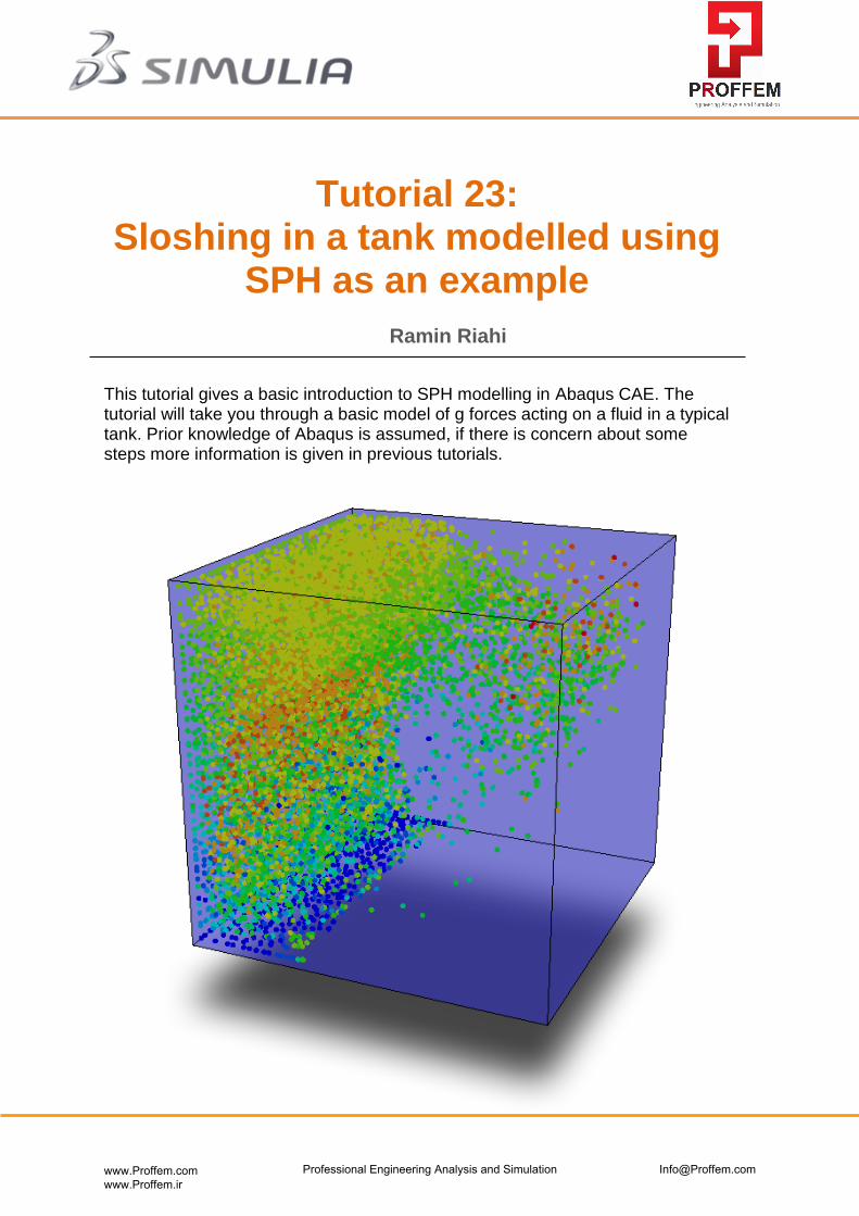
Tutorial 23:
Sloshing in a tank modelled using SPH as an example
Ramin Riahi
This tutorial gives a basic introduction to SPH modelling in Abaqus CAE. The tutorial will take you through a basic model of g forces acting on a fluid in a typical tank. Prior knowledge of Abaqus is assumed, if there is concern about some steps more information is given in previous tutorials.
www.Proffem.com www.Proffem.ir
Professional Engineering Analysis and Simulation [email protected]
2
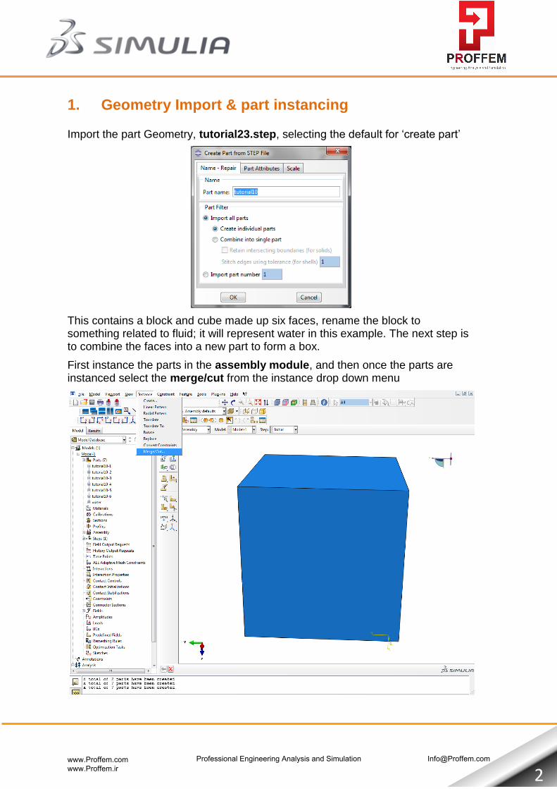
1. Geometry Import & part instancing
Import the part Geometry, tutorial23.step, selecting the default for ‘create part’
This contains a block and cube made up six faces, rename the block to something related to fluid; it will represent water in this example. The next step is to combine the faces into a new part to form a box.
First instance the parts in the assembly module, and then once the parts are instanced select the merge/cut from the instance drop down menu
www.Proffem.com www.Proffem.ir
Professional Engineering Analysis and Simulation [email protected]
3
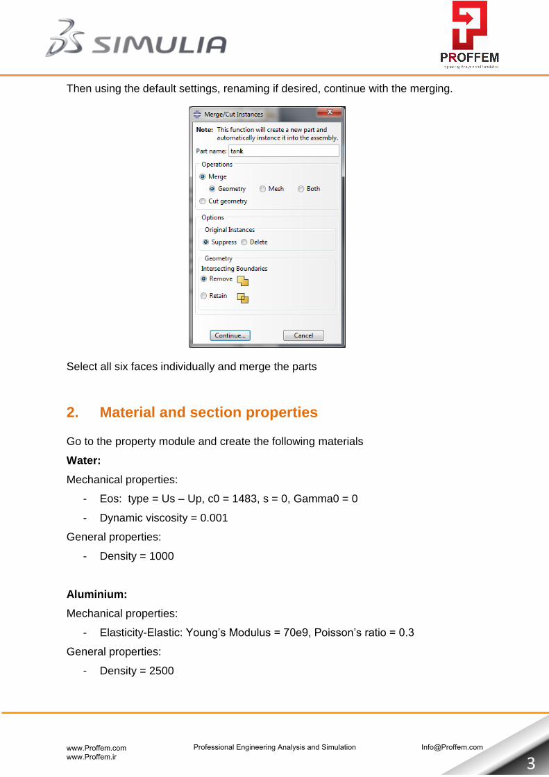
Then using the default settings, renaming if desired, continue with the merging.
Select all six faces individually and merge the parts
2. Material and section properties
Go to the property module and create the following materials
Water:
Mechanical properties:
- Eos: type = Us – Up, c0 = 1483, s = 0, Gamma0 = 0
- Dynamic viscosity = 0.001
General properties:
- Density = 1000
Aluminium:
Mechanical properties:
- Elasticity-Elastic: Young’s Modulus = 70e9, Poisson’s ratio = 0.3
General properties:
- Density = 2500
www.Proffem.com www.Proffem.ir
Professional Engineering Analysis and Simulation [email protected]

4
Then create a default solid homogeneous section for water and assign the section to the block. Then for the aluminium selection, select the ‘shell’ option with width of 0.002m and highlight the box
Note: When it comes to assigning sections ignore the 2D squares that merged into the box as they are no longer counted as part of the assembly.
3. Creating the steps
Go to the step module and create two new steps, for all steps in the model use the step option of ‘dynamic, explicit’
For the first step make the time period 0.5 seconds and 1 for the second step
www.Proffem.com www.Proffem.ir
Professional Engineering Analysis and Simulation [email protected]
5
4. Contacts
In the interaction module create a default all with self interaction and default global interaction property.
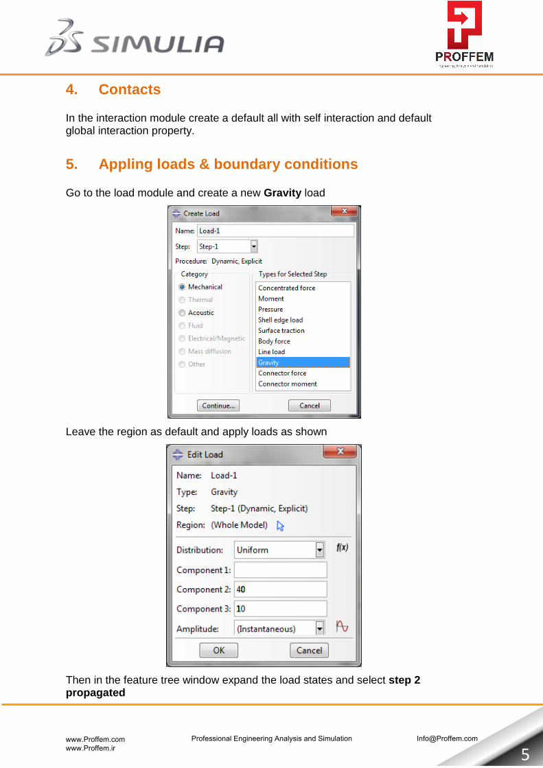
5. Appling loads & boundary conditions
Go to the load module and create a new Gravity load
Leave the region as default and apply loads as shown
Then in the feature tree window expand the load states and select step 2 propagated
www.Proffem.com www.Proffem.ir
Professional Engineering Analysis and Simulation [email protected]

6
And reduce the ‘component two’ load to zero
Lastly also apply an entcastre boundary conditions on the bottom four corners
6. Field output requests
Before meshing select the field output request and increase the interval to 500.
www.Proffem.com www.Proffem.ir
Professional Engineering Analysis and Simulation [email protected]

7
7. Meshing
In the meshing module mesh the aluminium tank and water block with spacings of about 0.05. Now assign an element type to the water
Change the element library to explicit and Conversion to particle to yes, with threshold = 0
www.Proffem.com www.Proffem.ir
Professional Engineering Analysis and Simulation [email protected]

8
8. Editing Keywords
Before testing the model the some lines must be added to the model keywords, select the edit keywords option on the feature tree window
www.Proffem.com www.Proffem.ir
Professional Engineering Analysis and Simulation [email protected]
9
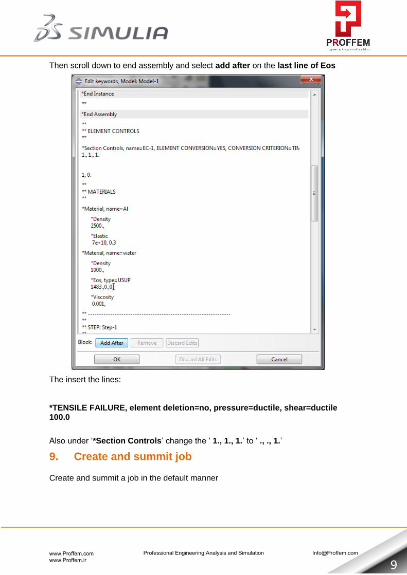
Then scroll down to end assembly and select add after on the last line of Eos
The insert the lines:
*TENSILE FAILURE, element deletion=no, pressure=ductile, shear=ductile 100.0
Also under ‘*Section Controls’ change the ‘ 1., 1., 1.’ to ‘ ., ., 1.’
9. Create and summit job
Create and summit a job in the default manner
www.Proffem.com www.Proffem.ir
Professional Engineering Analysis and Simulation [email protected]
10
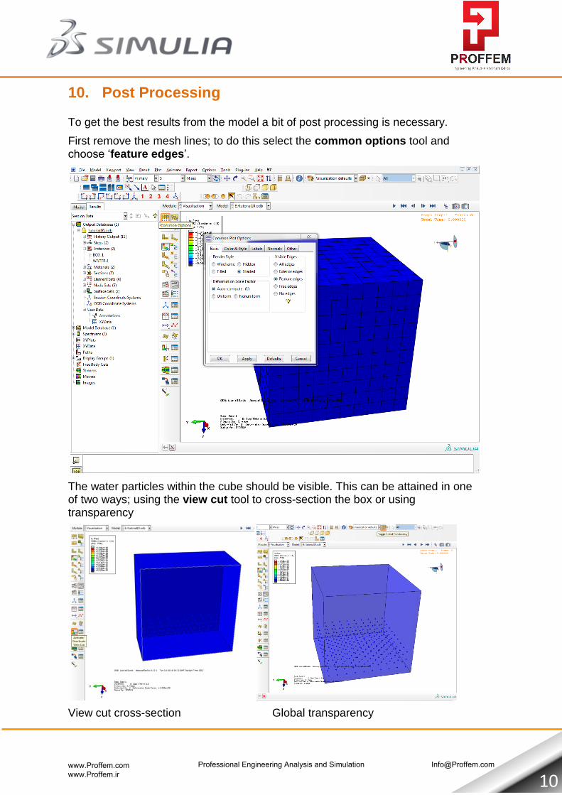
10. Post Processing
To get the best results from the model a bit of post processing is necessary.
First remove the mesh lines; to do this select the common options tool and choose ‘feature edges’.
The water particles within the cube should be visible. This can be attained in one of two ways; using the view cut tool to cross-section the box or using transparency
View cut cross-section Global transparency
www.Proffem.com www.Proffem.ir
Professional Engineering Analysis and Simulation [email protected]
11
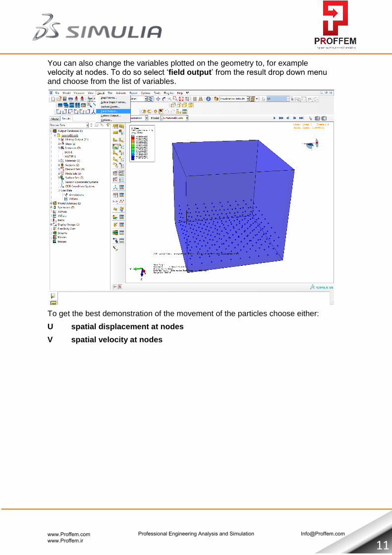
You can also change the variables plotted on the geometry to, for example velocity at nodes. To do so select ‘field output’ from the result drop down menu and choose from the list of variables.
To get the best demonstration of the movement of the particles choose either:
U spatial displacement at nodes
V spatial velocity at nodes
www.Proffem.com www.Proffem.ir
Professional Engineering Analysis and Simulation [email protected]