Turbulent boundary layers up to Re�=2500 studied through simulationand experiment

P. Schlatter,a� R. Örlü, Q. Li, G. Brethouwer, J. H. M. Fransson, A. V. Johansson,P. H. Alfredsson, and D. S. HenningsonLinné Flow Centre, KTH Mechanics, SE-100 44 Stockholm, Sweden

�Received 4 March 2009; accepted 24 April 2009; published online 20 May 2009�

Direct numerical simulations �DNSs� and experiments of a spatially developing zero-pressure-gradient turbulent boundary layer are presented up to Reynolds number Re�=2500, basedon momentum thickness � and free-stream velocity. For the first time direct comparisons of DNSand experiments of turbulent boundary layers at the same �computationally high and experimentallylow� Re� are given, showing excellent agreement in skin friction, mean velocity, and turbulentfluctuations. These results allow for a substantial reduction of the uncertainty of boundary-layerdata, and cross validate the numerical setup and experimental technique. The additional insight intothe flow provided by DNS clearly shows large-scale turbulent structures, which scale in outer unitsgrowing with Re�, spanning the whole boundary-layer height. © 2009 American Institute ofPhysics. �DOI: 10.1063/1.3139294�

The study and understanding of the turbulent flow closeto solid walls are a major topic in today’s research in fluiddynamics. Although in nature or technical applications thesurfaces are usually curved, possibly rough, and the meanflow is seldom exactly two dimensional, the spatially devel-oping, zero-pressure gradient turbulent boundary layer on asmooth, flat plate is an important canonical flow case fortheoretical, numerical, as well as experimental studies. Inrecent years, particularly careful experiments have been con-ducted. For instance, Österlund et al.1 performed extensivemeasurements of mean quantities in the minimum turbulencelevel �MTL� wind tunnel at KTH Stockholm using hot-wireanemometry and oil-film interferometry for Reynolds num-bers Re� �based on momentum thickness � and free-streamvelocity U�� ranging from 2530 to 27 300, with five mea-surement positions below Re�=6000. Recall that Re� pro-vides a measure of the streamwise position.

Direct numerical simulation �DNS� of turbulent flowsrelies on numerically resolving all relevant scales of motion.As the Reynolds number is getting larger the scale separationbetween the large and smallest scales is increasing consider-ably, limiting the Reynolds number attainable in DNS to lowvalues compared to experiments. As opposed to turbulentchannel2 and pipe flow,3 only few numerical results fromDNSs of turbulent boundary layers have been performed formedium or high �computational� Reynolds numbers. Themain reason is the extreme cost of spatial DNS due to thelong and consequently wide and high domains required, andthe loss of one homogeneous direction. Spalart’ssimulations4 using an innovative spatiotemporal approachprovided valuable data at Re�=300,670,1410, which havebecome a standard reference for numerical boundary-layerdata. Komminaho and Skote5 performed a spatial DNS up toRe�=700. The highest Reynolds number reached in DNS todate is the data reported by Ferrante and Elghobashi6 at

Re�=2900, however, obtained in a comparably short compu-tational domain in which the turbulence, in particular, thelarge-scale structures, may not be fully developed. Either thecomputational approaches were too different to the experi-ments or the Reynolds numbers were too low to make pos-sible a robust comparison.

For turbulent boundary layers, the Reynolds numberRe��2500 has to be considered at present high from a DNSpoint of view. On the other hand, a high-quality boundarylayer can be hard to establish and accurately measure at suchRe�, since low Reynolds number boundary-layer experi-ments need to be carried out at low velocities and for smalldistances from the leading edge. In the case of hot-wire mea-surements accurate calibration at low velocities is neededespecially for the near-wall measurements, whereas thechoice of tripping may affect the onset of transition to turbu-lence. The latter will affect the structure of the turbulencemainly in the outer part, leading to influences in the turbulentstatistics. Near the leading edge a pressure gradient is un-avoidable, but can be reduced to nearly zero by adjusting thegeometry of the setup. Turbulent boundary-layer data avail-able in literature have usually been taken in a range of Re�

by varying the free-stream velocity. The pressure gradienthas often been tuned for one specific case, since readjustmentof the pressure gradient is usually time consuming and there-fore not always realized. Thus some of the data available inthe literature are not taken in the optimal configuration forthe Re� in question.

Due to the difficulty of both DNS and experiments atReynolds numbers Re� on the order of a few thousand, thereis a comparably large spread of the existing data in literature,both for integral, mean, and fluctuating turbulent quantities,see, e.g., Ref. 7. There is thus a need for accurate and reliableDNS data of spatially developing turbulent boundary layerswith Re� to be compared to high-quality experimental re-sults. To this end, the inflow in the numerical simulationshould be positioned far enough upstream, i.e., comparableto where natural transition occurs, to ensure that the flowa�Electronic mail: pschlatt@mech.kth.se.

PHYSICS OF FLUIDS 21, 051702 �2009�

1070-6631/2009/21�5�/051702/4/$25.00 © 2009 American Institute of Physics21, 051702-1

Downloaded 19 Jan 2010 to 130.237.233.118. Redistribution subject to AIP license or copyright; see http://pof.aip.org/pof/copyright.jsp

reaches a fully developed, undisturbed equilibrium state fur-ther downstream.

The present letter reports a combined experimental andnumerical study of zero-pressure-gradient turbulent bound-ary layers, aiming to provide a well-validated data set per-taining to the dynamics of the mean and fluctuating turbulentquantities as a function of the downstream distance. Both theexperiments and simulations are performed with well estab-lished and reliable methods. In addition, by considering thesame generic flow case both experimentally and numerically,the sensitivity of the results to the respective method limita-tions, e.g., surface roughness, tripping technique, pressuregradients, and boundary conditions, etc., can be examined.

The simulations are performed using a fully spectralmethod to solve the time-dependent, incompressible Navier–Stokes equations.8 In the wall-parallel directions, Fourier se-ries with dealiasing are used whereas the wall-normal direc-tion is discretized with Chebyshev polynomials. Periodicboundary conditions in the streamwise direction are com-bined with a spatially developing boundary layer by adding a“fringe region” at the end of the domain. In this region, theoutflowing fluid is forced via a volume force to the laminarinflowing Blasius profile, located at Re�0

� =450 based on theinflow displacement thickness �0

�. A low-amplitude wall-normal trip force causes rapid laminar-turbulent transitionshortly downstream of the inlet. The chosen spectral methodprovides excellent accuracy and dispersion properties ascompared to low-order discretizations.

The computational domain is xL�yL�zL=3000�0�

�100�0��120�0

� with 3072�301�256 spectral collocationpoints in the streamwise, wall-normal, and spanwise direc-tions, respectively. The height and width of the computa-tional domain are chosen to be at least twice the largest 99%boundary-layer thickness, which reaches �99�45�0

� at Re�

=2500. The grid points are nonequidistantly distributed inthe wall-normal direction, with at least 15 collocation pointswithin the region y+�10. The grid resolution in viscousunits is then �x+��ymax

+ ��z+=17.9�8.6�9.6. Thestreamwise and spanwise resolutions are about a factor of 1.5lower than in the channel-flow study by Hoyas and Jiménez,2

however, to ensure adequacy of the chosen grid, we alsoperformed a resolution study based on the same box dimen-sions, but an increased number of grid points as 4096�385�480 showing only insignificant differences. Statis-tics are sampled over �t+�24 000 viscous time units, or 30in units of �99 /U� at Re�=2500. Owing to the high compu-tational cost of the simulations, the code is fully parallelizedrunning on O�1000� processors.

The turbulent boundary-layer measurements were per-formed in the MTL wind tunnel on a 7 m long flat plate atx=1.6 m from the leading edge, where the ceiling of thetunnel was adjusted for each measurement run to obtainzero-pressure-gradient conditions. The setup is similar to thatof Österlund.9 The free-stream velocity was 12.0 m/s and thestreamwise velocity component was measured by means ofhot-wire anemometry using a single wire probe. The sensorlength was 0.50 mm, corresponding to about 15 viscouslength units. This is sufficiently small in order not to observeeffects of spatial averaging on the measured fluctuation lev-

els in the near-wall region.10 A three-dimensional determin-istic surface roughness in combination with sandpaper wasused to trip the boundary layer in order to obtain a fixedtransition point. The skin friction was measured directly andindependent from the hot-wire measurements using oil-filminterferometry.11

The focus of the results presented here is on showingaveraged quantities and the fluctuations around that meanvalue. The considered case consists of a statistically two-dimensional boundary layer evolving in x and y, statisticallyhomogeneous in the spanwise direction z and stationary intime t. The Reynolds decomposition u= �u�+u�=U+u� isused, the brackets indicating the average in z and t. Based onthe mean velocity profile U�x ,y� the shear stress at the wallis obtained as �w�x�=��dU /dy� �y=0. Following the classicaltheory of turbulent boundary layers, the friction velocityU��w / provides the relevant velocity scale throughoutthe boundary layer, whereas the viscous length scale ��

/U� is the characteristic length at least close to the wall.The scaled quantities in wall scaling are thus written as, e.g.,U+=U /U� and y+=y /��.

In both the simulation and the experiment, the initiallylaminar boundary layer is tripped at approximately the samedistance from the leading edge in terms of Re�. Furtherdownstream of the tripping location, fully developed turbu-lence is established in which the boundary layer reaches anequilibrium state with the local production and dissipation ofturbulent kinetic energy balancing each other. In the simula-tions, the extent of the self-similar region downstream of thetripping can be estimated by considering the von Kármánintegral equation relating the local skin friction to the growthof the momentum thickness �. Based on this argument, theuseful region in the simulation may be defined as rangingfrom Re�=550 to 2500, corresponding to 75% of the totalcomputational domain. The peak skin friction Reynoldsnumber Re�=U��99 / is approximately 900 at Re�=2500.

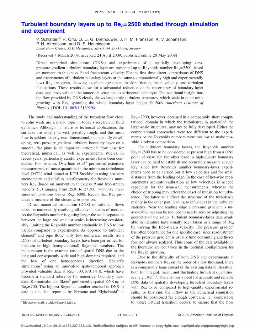
Characteristic mean quantities of the turbulent boundarylayer up to Re�=2500 are shown in Fig. 1. The skin frictionis shown as the friction velocity scaled by the free-streamvelocity, i.e., U� /U�=cf /2. Surprisingly, the simple corre-lation cf =0.024 Re�

�−1/4� �Ref. 12� provides an accurate fit tothe DNS data for the range of Reynolds numbers considered.The agreement with the new experimental measurement

(Uτ/U

∞)−

1

Reθ

500 1000 1500 2000 2500

14

16

18

20

22

24

H12

500 1000 1500 2000 2500

1.4

1.45

1.5

1.55

1.6

1.65

FIG. 1. Skin friction U� /U�=cf /2 and shape factor H12 as a function ofRe�. �—� Present DNS, ��� present experimental measurements. ��� DNSby Spalart �Ref. 4�. �¯� cf =0.024 Re�

�−1/4� �Ref. 12�, �– – –� correlation forH12 based on the composite profile suggested by Monkewitz et al. �Ref. 13�.

051702-2 Schlatter et al. Phys. Fluids 21, 051702 �2009�

Downloaded 19 Jan 2010 to 130.237.233.118. Redistribution subject to AIP license or copyright; see http://pof.aip.org/pof/copyright.jsp

point at Re�=2500 is very good. Recall that, experimentallythe skin friction is obtained using the oil-film technique11

independently of the velocity measurements. The shape fac-tor H12=�� /�, i.e., the ratio of displacement to momentumthickness, is also shown; this quantity provides a useful wayof characterizing the development state of the boundarylayer. It turns out that H12 is a sensitive indicator of thequality of the boundary-layer data at a given Re�. The agree-ment with both the new measurements and the shape factorbased on the composite velocity profile developed byMonkewitz et al.13 is again satisfactory. Note that the coef-ficients in the composite profile have been calibrated for ex-perimental boundary layers at higher Re� than the presentone. For comparison, the data points of the DNS by Spalart4

are also shown in Fig. 1. The skin friction is overpredictedby approximately 5% at the highest Re�=1410, whereas theshape factor is lower than the data obtained from both thecomposite profile and the present DNS. This might be a re-sidual effect of the spatiotemporal approach employed.

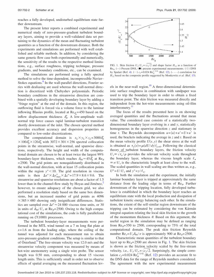
Profiles of the mean velocity scaled by viscous unitsU+�y+� obtained from both the present DNS and experimentsare shown in Fig. 2. The similarity at the highest Reynoldsnumber shown, Re�=2500, is excellent. However, there is adiscrepancy between the present simulation data and that ofSpalart at Re�=1410, probably due to a suspected lower ac-tual Re� in the latter simulation. In the wake region and thefree stream, Spalart’s results agree better with the presentdata at Re�=1000. In the near-wall region, all data collapsenicely on the linear relation U+=y+. The von Kármán coef-ficient � used to indicate the logarithmic region�1 /��log y++B is chosen as �=0.41 which seems to best fitthe data at this Re�. Inspection of the log-law indicator func-tion �=y+�dU+ /dy+� shows that the current DNS velocityprofile closely follows the composite profile proposed in Ref.13 up to y+=100. At Re�=2500, this wall-normal positioncan approximately be considered as the beginning of thewake region, in which the mean-flow gradient quickly risesto ��5.2 at y+�600. The minimum of � is at y+�70 witha value of 1 /��0.428 in good agreement with Ref. 13.

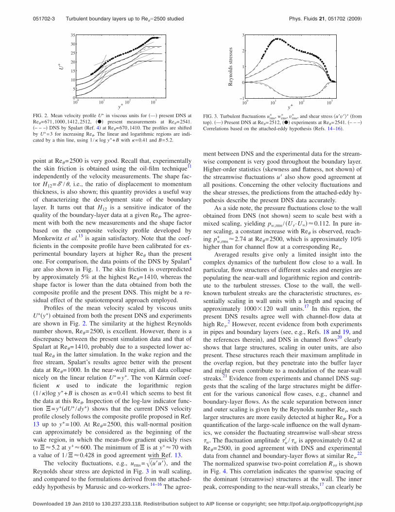
The velocity fluctuations, e.g., urms=�u�u��, and theReynolds shear stress are depicted in Fig. 3 in wall scaling,and compared to the formulations derived from the attached-eddy hypothesis by Marusic and co-workers.14–16 The agree-

ment between DNS and the experimental data for the stream-wise component is very good throughout the boundary layer.Higher-order statistics �skewness and flatness, not shown� ofthe streamwise fluctuations u� also show good agreement atall positions. Concerning the other velocity fluctuations andthe shear stresses, the predictions from the attached-eddy hy-pothesis describe the present DNS data accurately.

As a side note, the pressure fluctuations close to the wallobtained from DNS �not shown� seem to scale best with amixed scaling, yielding pw,rms / �U� ·U���0.112. In pure in-ner scaling, a constant increase with Re� is observed, reach-ing pw,rms

+ �2.74 at Re�=2500, which is approximately 10%higher than for channel flow at a corresponding Re�.

Averaged results give only a limited insight into thecomplex dynamics of the turbulent flow close to a wall. Inparticular, flow structures of different scales and energies arepopulating the near-wall and logarithmic region and contrib-ute to the turbulent stresses. Close to the wall, the well-known turbulent streaks are the characteristic structures, es-sentially scaling in wall units with a length and spacing ofapproximately 1000�120 wall units.17 In this region, thepresent DNS results agree well with channel-flow data athigh Re�.

2 However, recent evidence from both experimentsin pipes and boundary layers �see, e.g., Refs. 18 and 19, andthe references therein�, and DNS in channel flows20 clearlyshows that large structures, scaling in outer units, are alsopresent. These structures reach their maximum amplitude inthe overlap region, but they penetrate into the buffer layerand might even contribute to a modulation of the near-wallstreaks.21 Evidence from experiments and channel DNS sug-gests that the scaling of the large structures might be differ-ent for the various canonical flow cases, e.g., channel andboundary-layer flows. As the scale separation between innerand outer scaling is given by the Reynolds number Re�, suchlarger structures are more easily detected at higher Re�. For aquantification of the large-scale influence on the wall dynam-ics, we consider the fluctuating streamwise wall-shear stress�w. The fluctuation amplitude �w� /�w is approximately 0.42 atRe�=2500, in good agreement with DNS and experimentaldata from channel and boundary-layer flows at similar Re�.

22

The normalized spanwise two-point correlation R�� is shownin Fig. 4. This correlation indicates the spanwise spacing ofthe dominant �streamwise� structures at the wall. The innerpeak, corresponding to the near-wall streaks,17 can clearly be

y+

U+

100

101

102

103

0

5

10

15

20

25

30

35

FIG. 2. Mean velocity profile U+ in viscous units for �—� present DNS atRe�=671,1000,1412,2512, ��� present measurements at Re�=2541.�– – –� DNS by Spalart �Ref. 4� at Re�=670,1410. The profiles are shiftedby U+=3 for increasing Re�. The linear and logarithmic regions are indi-cated by a thin line, using 1 /� log y++B with �=0.41 and B=5.2.

y+

Rey

nold

sst

ress

es

100

101

102

103

−1

0

1

2

3

FIG. 3. Turbulent fluctuations urms+ , wrms

+ , vrms+ , and shear stress �u�v��+ �from

top�. �—� Present DNS at Re�=2512, ��� experiments at Re�=2541. �– – –�Correlations based on the attached-eddy hypothesis �Refs. 14–16�.

051702-3 Turbulent boundary layers up to Re� 2500 studied Phys. Fluids 21, 051702 �2009�

Downloaded 19 Jan 2010 to 130.237.233.118. Redistribution subject to AIP license or copyright; see http://pof.aip.org/pof/copyright.jsp

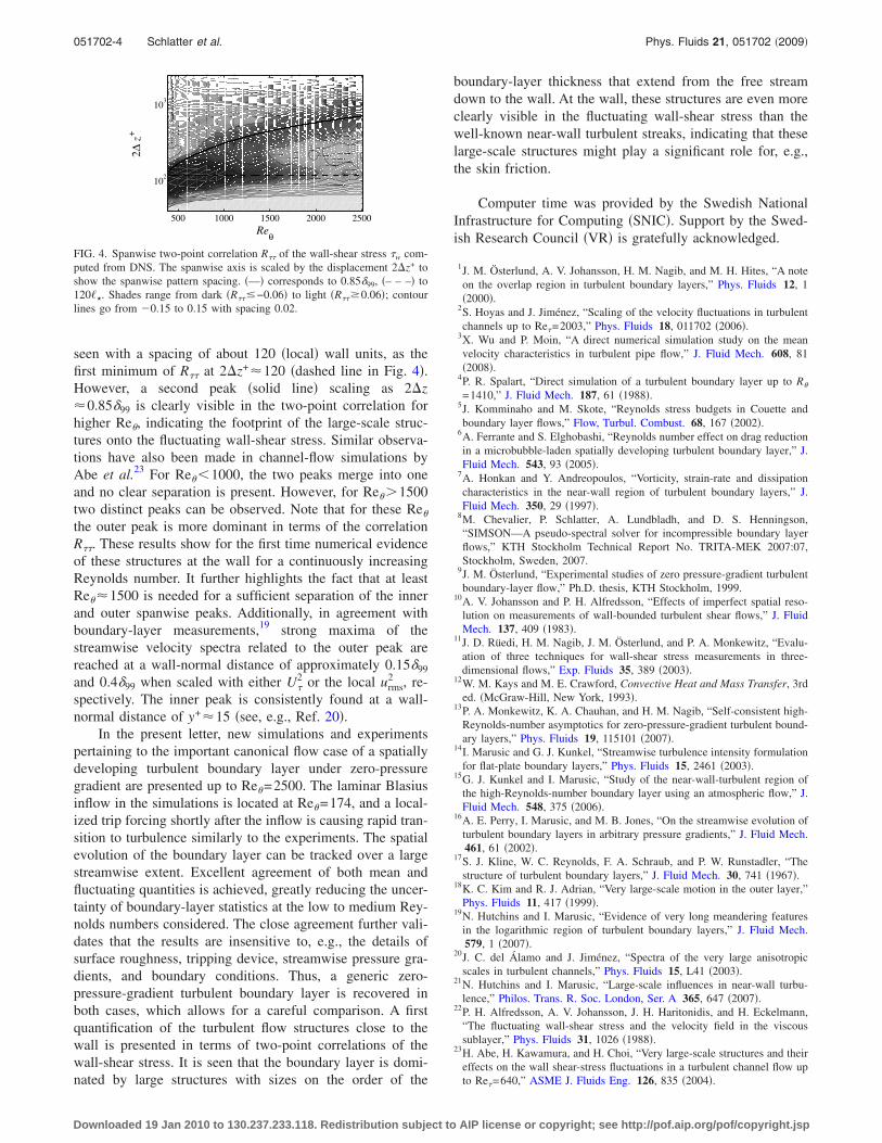
seen with a spacing of about 120 �local� wall units, as thefirst minimum of R�� at 2�z+�120 �dashed line in Fig. 4�.However, a second peak �solid line� scaling as 2�z�0.85�99 is clearly visible in the two-point correlation forhigher Re�, indicating the footprint of the large-scale struc-tures onto the fluctuating wall-shear stress. Similar observa-tions have also been made in channel-flow simulations byAbe et al.23 For Re��1000, the two peaks merge into oneand no clear separation is present. However, for Re��1500two distinct peaks can be observed. Note that for these Re�

the outer peak is more dominant in terms of the correlationR��. These results show for the first time numerical evidenceof these structures at the wall for a continuously increasingReynolds number. It further highlights the fact that at leastRe��1500 is needed for a sufficient separation of the innerand outer spanwise peaks. Additionally, in agreement withboundary-layer measurements,19 strong maxima of thestreamwise velocity spectra related to the outer peak arereached at a wall-normal distance of approximately 0.15�99

and 0.4�99 when scaled with either U�2 or the local urms

2 , re-spectively. The inner peak is consistently found at a wall-normal distance of y+�15 �see, e.g., Ref. 20�.

In the present letter, new simulations and experimentspertaining to the important canonical flow case of a spatiallydeveloping turbulent boundary layer under zero-pressuregradient are presented up to Re�=2500. The laminar Blasiusinflow in the simulations is located at Re�=174, and a local-ized trip forcing shortly after the inflow is causing rapid tran-sition to turbulence similarly to the experiments. The spatialevolution of the boundary layer can be tracked over a largestreamwise extent. Excellent agreement of both mean andfluctuating quantities is achieved, greatly reducing the uncer-tainty of boundary-layer statistics at the low to medium Rey-nolds numbers considered. The close agreement further vali-dates that the results are insensitive to, e.g., the details ofsurface roughness, tripping device, streamwise pressure gra-dients, and boundary conditions. Thus, a generic zero-pressure-gradient turbulent boundary layer is recovered inboth cases, which allows for a careful comparison. A firstquantification of the turbulent flow structures close to thewall is presented in terms of two-point correlations of thewall-shear stress. It is seen that the boundary layer is domi-nated by large structures with sizes on the order of the

boundary-layer thickness that extend from the free streamdown to the wall. At the wall, these structures are even moreclearly visible in the fluctuating wall-shear stress than thewell-known near-wall turbulent streaks, indicating that theselarge-scale structures might play a significant role for, e.g.,the skin friction.

Computer time was provided by the Swedish NationalInfrastructure for Computing �SNIC�. Support by the Swed-ish Research Council �VR� is gratefully acknowledged.

1J. M. Österlund, A. V. Johansson, H. M. Nagib, and M. H. Hites, “A noteon the overlap region in turbulent boundary layers,” Phys. Fluids 12, 1�2000�.

2S. Hoyas and J. Jiménez, “Scaling of the velocity fluctuations in turbulentchannels up to Re�=2003,” Phys. Fluids 18, 011702 �2006�.

3X. Wu and P. Moin, “A direct numerical simulation study on the meanvelocity characteristics in turbulent pipe flow,” J. Fluid Mech. 608, 81�2008�.

4P. R. Spalart, “Direct simulation of a turbulent boundary layer up to R�

=1410,” J. Fluid Mech. 187, 61 �1988�.5J. Komminaho and M. Skote, “Reynolds stress budgets in Couette andboundary layer flows,” Flow, Turbul. Combust. 68, 167 �2002�.

6A. Ferrante and S. Elghobashi, “Reynolds number effect on drag reductionin a microbubble-laden spatially developing turbulent boundary layer,” J.Fluid Mech. 543, 93 �2005�.

7A. Honkan and Y. Andreopoulos, “Vorticity, strain-rate and dissipationcharacteristics in the near-wall region of turbulent boundary layers,” J.Fluid Mech. 350, 29 �1997�.

8M. Chevalier, P. Schlatter, A. Lundbladh, and D. S. Henningson,“SIMSON—A pseudo-spectral solver for incompressible boundary layerflows,” KTH Stockholm Technical Report No. TRITA-MEK 2007:07,Stockholm, Sweden, 2007.

9J. M. Österlund, “Experimental studies of zero pressure-gradient turbulentboundary-layer flow,” Ph.D. thesis, KTH Stockholm, 1999.

10A. V. Johansson and P. H. Alfredsson, “Effects of imperfect spatial reso-lution on measurements of wall-bounded turbulent shear flows,” J. FluidMech. 137, 409 �1983�.

11J. D. Rüedi, H. M. Nagib, J. M. Österlund, and P. A. Monkewitz, “Evalu-ation of three techniques for wall-shear stress measurements in three-dimensional flows,” Exp. Fluids 35, 389 �2003�.

12W. M. Kays and M. E. Crawford, Convective Heat and Mass Transfer, 3rded. �McGraw-Hill, New York, 1993�.

13P. A. Monkewitz, K. A. Chauhan, and H. M. Nagib, “Self-consistent high-Reynolds-number asymptotics for zero-pressure-gradient turbulent bound-ary layers,” Phys. Fluids 19, 115101 �2007�.

14I. Marusic and G. J. Kunkel, “Streamwise turbulence intensity formulationfor flat-plate boundary layers,” Phys. Fluids 15, 2461 �2003�.

15G. J. Kunkel and I. Marusic, “Study of the near-wall-turbulent region ofthe high-Reynolds-number boundary layer using an atmospheric flow,” J.Fluid Mech. 548, 375 �2006�.

16A. E. Perry, I. Marusic, and M. B. Jones, “On the streamwise evolution ofturbulent boundary layers in arbitrary pressure gradients,” J. Fluid Mech.461, 61 �2002�.

17S. J. Kline, W. C. Reynolds, F. A. Schraub, and P. W. Runstadler, “Thestructure of turbulent boundary layers,” J. Fluid Mech. 30, 741 �1967�.

18K. C. Kim and R. J. Adrian, “Very large-scale motion in the outer layer,”Phys. Fluids 11, 417 �1999�.

19N. Hutchins and I. Marusic, “Evidence of very long meandering featuresin the logarithmic region of turbulent boundary layers,” J. Fluid Mech.579, 1 �2007�.

20J. C. del Álamo and J. Jiménez, “Spectra of the very large anisotropicscales in turbulent channels,” Phys. Fluids 15, L41 �2003�.

21N. Hutchins and I. Marusic, “Large-scale influences in near-wall turbu-lence,” Philos. Trans. R. Soc. London, Ser. A 365, 647 �2007�.

22P. H. Alfredsson, A. V. Johansson, J. H. Haritonidis, and H. Eckelmann,“The fluctuating wall-shear stress and the velocity field in the viscoussublayer,” Phys. Fluids 31, 1026 �1988�.

23H. Abe, H. Kawamura, and H. Choi, “Very large-scale structures and theireffects on the wall shear-stress fluctuations in a turbulent channel flow upto Re�=640,” ASME J. Fluids Eng. 126, 835 �2004�.

Reθ

2∆z+

500 1000 1500 2000 2500

102

103

FIG. 4. Spanwise two-point correlation R�� of the wall-shear stress �w com-puted from DNS. The spanwise axis is scaled by the displacement 2�z+ toshow the spanwise pattern spacing. �—� corresponds to 0.85�99, �– – –� to120��. Shades range from dark �R���−0.06� to light �R���0.06�; contourlines go from �0.15 to 0.15 with spacing 0.02.

051702-4 Schlatter et al. Phys. Fluids 21, 051702 �2009�

Downloaded 19 Jan 2010 to 130.237.233.118. Redistribution subject to AIP license or copyright; see http://pof.aip.org/pof/copyright.jsp