Drag reduction of turbulent boundary layers by means ofgrooved surfacesCitation for published version (APA):Pulles, C. J. A. (1988). Drag reduction of turbulent boundary layers by means of grooved surfaces. Eindhoven:Technische Universiteit Eindhoven. https://doi.org/10.6100/IR280307

DOI:10.6100/IR280307

Document status and date:Published: 01/01/1988

Document Version:Publisher’s PDF, also known as Version of Record (includes final page, issue and volume numbers)

Please check the document version of this publication:

• A submitted manuscript is the version of the article upon submission and before peer-review. There can beimportant differences between the submitted version and the official published version of record. Peopleinterested in the research are advised to contact the author for the final version of the publication, or visit theDOI to the publisher's website.• The final author version and the galley proof are versions of the publication after peer review.• The final published version features the final layout of the paper including the volume, issue and pagenumbers.Link to publication

General rightsCopyright and moral rights for the publications made accessible in the public portal are retained by the authors and/or other copyright ownersand it is a condition of accessing publications that users recognise and abide by the legal requirements associated with these rights.

• Users may download and print one copy of any publication from the public portal for the purpose of private study or research. • You may not further distribute the material or use it for any profit-making activity or commercial gain • You may freely distribute the URL identifying the publication in the public portal.

If the publication is distributed under the terms of Article 25fa of the Dutch Copyright Act, indicated by the “Taverne” license above, pleasefollow below link for the End User Agreement:

www.tue.nl/taverne

Take down policyIf you believe that this document breaches copyright please contact us at:

openaccess@tue.nl

providing details and we will investigate your claim.

Download date: 26. Jan. 2020

DRAG REDUCTION

OF

TURBULENT BOUNDARY LAYERS

BY MEANS OF GROOVED SURFACES

C:J.A.PULLES

DRAG REDUCTION

OF

TURBULENT BOUNDARY LAYERS

BY MEANS Oir GROOVED SURFACES

Proefschrift

ter verkrijging vim de graad van doctor aan de Technische Universiteit Eindhoven, op gezag

I

van de Rector Magnificus, prof. dr. F.N. Hooge, I

voor een commissie aangewezen door het College van Dekanen i ~ het openbaar te verdedigen op

vrijdag 4 maart 1988 te 16.00 uur

door

CORNELIS J~HANNES ADRIANUS PULLES

geboren te Eindhoven

I d k: Oissertatiedrukkerij Wibro. Helmond.

Dit proefschrift is goedgekeurd door de promotoren:

Dr. ir. G. Ooms

en Prof. dr. ir. G. Vossers

Co-promotor: Dr. K. Krishna Prasad

This research has been supported by the Nederlands Technology

Foundation (STW) as part of the program of the Foundation for Fundamental Research on Matter (FOM)

Drag reductlon of turbulent boundary layers

bv means of grooved surfaces.

Contents

List of symbols.

Chapter 1 Introduetion.

§ 1 . 1 Historie review.

§ 1.2 Short deseription of smooth wall

turbulent boundary layer.

§ 1.3 Strueture of this thesis.

Chapter 2 Summary of existing ideas. theories and

5

7

experiments. 9

§ 2.1 Survey of different means of obtaining

drag reduetion. 9

§ 2.2 Ideas and theories eoneerning

drag reduetion. 12

§ 2 . 3 Experimental results from literature

eoneerning drag reduetion by means

of mierogrooves. 23

Chapter 3 Experimental setup. 29

§ 3.1 Water ehannel. 29

§ 3.2 Measurement system. 34

§ 3.3 Deseription of the roughness types. 37

Chapter 4 Point measurements. 42

§ 4.1 Introduetion. 42

§ 4.2 Profiles. 43

§ 4.3 Detailed point measurements. 51

§ 4.4 Conelusions. 62

Chapter 5 Hydrogen bubble visualisation. 63

§ 5.1 Introduetion. 63

§ 5.2 Deseription of the experimental set-up. 65

§ 5.3 Some tests of the method. 70

§ 5.4 Results of the automated visualisation

experiment.

§ 5.5 Results of the visualisation with

LDA measurements.

§ 5.6 Conelusions.

Chapter 6 Drag measurements.

iii

75

77

89

93

§ 6.1 Survey of different methods of

measuring drag.

§ 6 . 1.1 Indirect methods.

§ 6 . 1.2 Direct methods.

§ 6.2 Drag balance Delft.

§ 6.3 Design considerations of the

drag balance.

§ 6 .4 Some additional design formula of

the balance.

§ 6.5 Sensor.

§ 6.6 Measurements and results.

Chapter 7 Discussion and suggestions for

further research.

Appendix A rhe method of Head applied to the

water channel flow.

Appendix B rhe accuracy of the spanwise

correlation function.

References.

Summary.

Samenva t Ung.

Dankwoord.

Curriculum vitae.

iv

93

93

97

99

99

104

110

110

115

119

121

126

131

132

133

133

List of symbols.

Roman symbols.

A

a

B

b

Cf

D

H

h

k

I!

P

P p

U

u

u

* u

U .. v

v

v

w x

y

* y

z

van Driest constant

ratio between Reynolds shear stress

and turbulent intensity

constant in Spaldings formuia

groove width

friction coefficient

pipe diameter

shape factor of boundary layer 9/ó*

groove height

trigger level in burst detection procedure

mixing length

pressure

pressure gradient parameter

velocity component in the direction of the

free stream direction.

fluctuating part of U. U-U rms of U

shear stress velocity ~ w

free stream flow velocity

velocity component at right angles with the

surface

fluctuating part of V. V-V rms of V

spanwise velocity component

distance from start of boundary layer

vertical distance from surface

viscous length v/u*

spanwise distance

Greek symbols.

ó boundary layer thickness

v

[m]

[m]

[m]

[mis]

[mis]

[mis]

[mis]

[mis]

[mis]

[mis]

[mis]

[mis]

Cm] Cm] Cm] Cm]

Cm]

6* displacement thickness Cm]

E- dissipation of turbulent energy [J/kg]

Tl dynamic viscosi ty . [kg/m s]

e momentum loss thickness Cm]

K. von Karman's konstant 0.41

À. low speed streak spacing Cm]

kinematic 2 v viscosity [m /s]

p density [kg/m3 ]

T total shear stress [N/m2]

Tl viscous shear stress [N/m2]

Tt turbulent shear stress [N/m2]

T wall shear stress [N/m2] w

Superscripts

(overbar) ave rage value . time or ensemble ave rage

+ quantity made dimensionless by wall variables TW' pand v

vi

Chapter Introduction.

§ 1.1 Historie review.

Time af ter time nature provides us withunexpected phenomena.

Although very common, turbulence should be reckoned among them. It is

surprising to observe how a smooth laminar flow through a pipe, sudden

ly becomes chaotic. Osborne Reynolds [lB9S] was the first to investi­

gate this phenomenon in some depth .

During the years most schol ars used the obvious random nature of

turbulence in order to f ind a sui table model. WeIl known is the

reasoning of Kolmogorov [1941] which provides an estimate of the

length and timescales involved. It rests heavily on the assumption of

scale invariance of turbulence.

During the last two decades it became clear that turbulence is

not as random as a first glance would suggest. Patterns are detected

in wall boundary layers, jetsand pipe flow [see eg Kunen 19B4]. And

literature is filled with descriptions of "bursts", "horse-shoe vorti­

ces", "low speed streaks" and other coherent structures, which were

detected by experimenters. Some of those structures are also observed

in other turbulent flows. like turbulent jets and free shear layers.

'Still more recent is the application of mathematical ideas of

strange at tractors and chaotic systems to turbulence [Eckmann 19B1 J. No unification with the former ideas is apparent yet.

i Also noted was the easy way turbulence was modified. for

instanee by suction or blowing and numerous other devices . Apparently

turbulence is a very complex phenomenon and therefore i t can be

influenced in many ways. T~ date no satisfactory theory describing

turbulence is available but most scholars believe that all the

necessary information is contained in the Navier-Stokes equations. Up

till now no evidence to the contrary is available. Moreover, the

direct simulation of very simple turbulent flows is just within reach

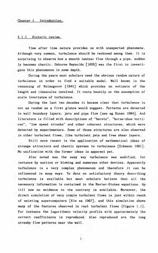
of existing supercomputers [Kim ea 19B7J. and this simulation shows

many of the features observed in real turbulent flows (figure 1.1).

For instanee the logarithmic velocity profile with approximately the

correct coefficients is reproduced. Also reproduced are the long

streaky flow patterns near the wall.

3.0.----------------, 2.S

w~..... .. ~: :::.;..~.~.~: .. --l.--~.~.-..-:=

~,: -" ,

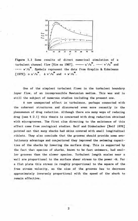
Figure 1.1 Some resul ts of direct numerical simulation of a

turbulent channel flow [Kim ea 1987] . ---u'/u*, ---- v'/u* and

•••• w'/u*. Symbols represent the data from Kreplin & Eckelmann * * * [1979] : 0 u'/u, A v'Ju and + w'/u .

One of the simplest turbulentflows is the turbulent boundary

layer flow. of an incompressible Newtonian medium. This was and is

still the subject of numerous studies including the present one.

A new unexpected effect in turbulence, perhaps connected wi th

the coherent structures and discovered even more recently is the

phenomenon of drag reduction. Although there are many ways of reducing

drag (see § 2.1) this thesis is concerned with drag reduction obtained

with microgrooves. The first clue directing to the existence of this

effect came from zoological studies. Reif and Dinkelacker [Reif 1976]

pointed out thàt many sharks had skins covered with small longitudinal

riblets. They also conclude that the grooves should provide sorne evo­

lutionary advantage and conjectured they improved the swimrning capaci­

ties of the sharks by lowering the surface drag. This is supported by

the fact that species of sharks, known to be fast swimmers, had smal­

ler grooves than the slower species. Turbulent length scales near a

wall are proportional to the surface shear stress tothe power~. For

a flat plate this stress is roughly proportional to the square of the

free stream veloei ty, so the size of the grooves has to decrease

approximately inversely proportional wi th the speed of the shark to

remain effective.

2

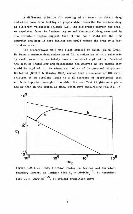
A different stimulus for seeking af ter means to obtain drag

reduction came from looking at graphs which describe the surface drag

at different velocities (figure 1.2). The difference between the drag,

extrapolated from the laminar regime and the actual drag measured in

the turbulent regime suggest that if one could stabilize the flow

somewhat and keep it more laminar one could reduce the drag by a fac­

tor 4 or more .

The microgrooved wall was first studied by Walsh [Walsh 1976J.

He found a maximum drag reduction of 7%. A reduction of this relativi­

ly small amount can certainly have a technica I application. Provided

the cost of installing and maintaining the grooves is low enough they

could be applied to the wings and bodies of large-sized airplanes.

Bertelrud [Savill & Rhyming 1987J argues that a decrease of 10% skin­

friction of an airplane leads to a 1% decrease of operational cost

which is important enough to consider its use. Test flights were plan­

ned by NASA in the course of 1986, which gave encouraging results. In

1Ö3r---------------------------------~

Flgure 1.2 Local skin friction factor in laminar and turbulent -'A

boundary layers. a: laminar flow Cf = .646.Rex ' b: turbulent

-1/5 . flow Cf = .0592-Re ,c: typical transition curve.

3

september 1987, the first "International Conference on turbulent drag

Reduction by passive Means" took pi ace in London. About half of the

presentations considered the use of microgrooves.

As fuel consumption is a major operational cost of supertankers

and surface drag is a large part of the total drag experienced by the

ship ploughing through the sea, microgrooved hulls could be of certain

importance. It remains to be established, however, whether it is possi

bIe to maintain the quality of the grooves for longer periods of time

under the adverse conditions at sea. And of course, in a world in

which the value of currency can change by 50% or more, 5% drag reduc­

tion will only be a major factor determining economie success or fail­

ure of an application in very special cases.

In the present study we will not pay further attent ion to sharks

and economie benefits of microgrooves. Instead we wil! approach the

problem from a different angle. Drag reduction by means of micro­

grooves is not only interesting because of possible technica I applica­

tions , but i t provides also an opportuni ty to refine and test the

theories of anormal smooth wall boundary layer as weIl. We will try

to illuminate the mechanism responsible for drag reduction. By doing

this we will have scrutinized simultaneously the mechanisms for

momentum transfer in a no rma I boundary layer. We will do this mainly

wi th experimental means as opposed to theoretical and mathematical

approaches. This has two reasons . Firstly, much experimental data

needed to conceive a coherent intui tive picture of the influence of

those grooves on the flow are still lacking and secondly a theoretical

approach seems less prom,l.sing, because no theory exists today which

can predict drag in a normal turbulent boundary layer with an accuracy

of a few per cent without the help of empirically determined

constants.

It is probably wise to regard this thesis as a reconnaissance

study in which the feasibility of studying micro grooved induced drag

reduction at 10w Reynolds numbers is demonstrated. During the last

four years the instrUments needed for the experiments (the water chan­

nel, the drag balance, the laser-doppler anemometer (LDA) and the

computerized visualisation) were developed and checked out. These are

no scientific resul ts on their own but i t was very necessary and i t

took its time to do it. Further resarch wil I prof it from these funda­

mental achievements.

...

§ 1.2 Short description of smoöth wall turbulent boundary layer.

From the existing I iterature about a turbulent boundary layer.

the theories and the experimental data the following description of a

turbulent boundary layer can be distilled [see e.g. Hinze 1975].

Generally a turbulent boundary layer can be separated into four

distinctly different parts. They can be characterized by the proper­

ties of the mean velocity profile or by the observed flow structures.

For the properties of the mean velocity profile some theoretical jus­

tification can be given but theories describing and predicting the

flow structure are very incomplete and the subject of much contempora­

ry resarch. The distinctive regions are:

I y + < 5 The viscous sublayer. Very close to the wall exists a

reg ion in which the viscous forces dominate the momentum transport.

The vertical velocity component is strongly damped and the flow is

near ly two dimensional. In this region the mean veloei ty is a

linear function of the distance from the surface.

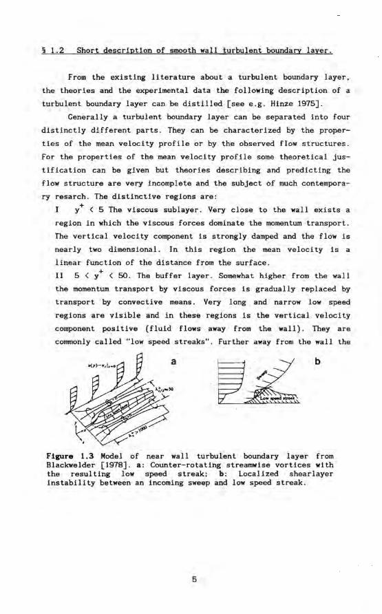
11 5 < y+ < 50. The buffer layer. Somewhat higher from the wall

the momentum transport by vlscous forces is gradually replaced by

transport by convective means. Very long and narrow low speed

reglons are visible and in these reglons is the vertical velocity

component positive (fluid flows away from the wall). They are

commonly called "low speed streaks". Further away from the wal! the

.b

Flgure 1.3 Model of near wall turbulent boundary layer from Blackwelder [1978]. a: Counter-rotating streamwise vortices wlth the resul ting low speed streak; b: Localized shearlayer instability between an incoming sweep and low speed streak.

5

shape of these regions becomes more irregular. On top of these low

speed streaks vortices are generated. The ends of the vortices are

heavily sheared and appear as longitudinal vortices along the

streaks. These structures are cal led horse-shoe vortices. The low

speed streak sometimes ends abruptly and fluid is then replaced by

faster moving fluid from higher up in the boundary layer. At y+ of

about 50 the turbulent momentum transport reaches a rather broad

maximum. In figure 1.3 a somewhat different view is pictured by

Blackwelder [1978]. + -

III y > 50. U < .8 Uro The logarithmic region. From that height to

the height where the mean flow veloei ty ij is about . B times the

free stream veloei ty the transport slowly decreases again. Flow

structures in this region are layers of vortices inclined at 45

degrees. This reg ion is characterized by a logarithmic dependenee

of the mean velocity on the height. and is therefore called the

logarithmic region. It is generally assumed that up to this height

the wall shear stress is the main parameter which controls the flow

and consequently all physical quantities can be made dimensionless

with the shear stress and the properties of the flow medium.

IV .8 U < ij. The outer layer. Above the logarithmic region the ro

outer layer is situated. Here the flow is determined by the

pressure gradient and the upstream hlstory of the boundary layer.

The flow is intermittently turbulent and laminar. Physical

quanti ties tend to scale on boundary layer thickness. I t can be

shown from dimensional analysis that the existence of the viscous

sublayer and the outer layer imply the existence of a reg ion where

the mean velocity follows a logarithmic curve. The precise shape of

the velocity profile depends on the pressure gradient. but the

velocity tends smoothly and asymptotically to the free stream

velocity.

The layers. however. do not exist independently. Extreme dP pressure gradients cen cause relaminarisation Cdx < 0) or separation

C: ) 0). thus affecting the boundary layer as a whole but under

normal conditions the individual layer only provides the boundary

conditions for its neighbours.

It is only fair to note that the description of the turbulent

6

boundary layer in tenns of coherent structures is subject to much

debate. As yet no complete consensus has been reached. Al though the

structures here described are detected by many observers, discussion

centers around their relevance to momentum transport or their

relevance as building blocks of turbulence. As long as no firm picture

of a smooth wall turbulent boundary layer emerges, backed by a more or

less solid mathematical theory the interpretation of changes in the

boundary layer above microgrooves can only be tentative.

§ 1.3 Structure of this thesis.

The basic idea used in this thesis about the mechanism behind

the microgrooved drag reduction is: the grooves influence in some way

the convers ion of viscous to turbulent momentum transport thus

hindering the momentum transfer as a whoie. This affects particularly

the viscous sublayer and the buffer layer. It is expected but yet to

be proven. tha t the logar i thrnic layer merely adjusts itself to the

lower momentum flux passed by the layer below. The outer layer should

remain entirely unaffected by the microgrooves and alternatively.

except under very extreme situations, the outer layer eannot affect

the drag reduction mechanism of the microgrooves.

The details of the dragreducing meehanisms are unclear but

microgroove drag reduction itself is confirmed by several experiments

[Saviii & Rhyrning 1987] . From the optimal size of the grooves. experi­

mental studies (particularly flow visualisation. for instance Offen

and Kline [1973]). and theoretical considerations we can conclude that

the behaviour of the total turbulent layer is detennined to a large

extent by the viseous sublayer and the bufferlayer. The theories could

be developed along several ideas. which are discussed in chapter 2.

In our experiments we will thus pay close attention to the flow

layer very close to the wall. In the present study we will show that

the turbulent boundary layer maintains largely its structure above a

drag reducing grooved wal!. For instance. the logari thrnic veloei ty

profile is still present and near the wall low speed streaks are still

diseernible. When looked at in more detail. however. some small

quantitative changes can be found. The aim of the present study is to

highlight the differenees and to compare them against the incomplete

7

ideas offered about the subject of mlcrogroove drag reduction. .

The general outline of the experimental equipment is discussed

in chapter 3. The measurementsthemselves can he roughly divided into

three categories:

I Point measurements (chapter 4), which give accurate information

on the physical quantities in the flow at a single point.

II Visualisation studies (chapter 5), which provide less accurate

information over a more extended area of the flow .

111 Direct drag measurements (chapter 6) which give the yardstick

for scaling the different boundary layers.

Ihis subdivision cannot be made too strict because sometimes it

is just the combination of the information provided by the different

methods which is particularly valuable. If this occurs we will try to

point out this explicitly.

Ihe implications of the experimental results will be discussed

in"chapter 7.

B

Chapter 2 Summary ofexisting ideas, theories and experiments.

§ 2.1 Survey of different means of obtaining dragreduction.

There are many ways in which turbulence can he influenced and

most modifications have in principle the potential to achieve drag

reduction . We can split these attempts in two categories: the use of

active or passive devices. Active devices are those which use a sensor

to detect a particular event (eg separation or a turbulent burst) and

trigger an actuator to act upon the flow. This feedback is absent in

passive devices.

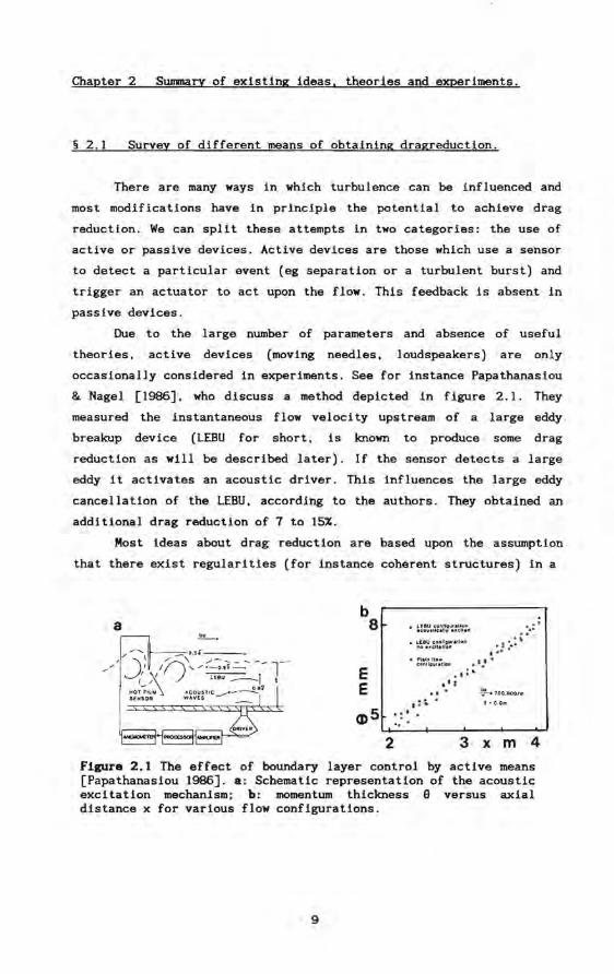
Due to the large number of parameters and absence of useful

theories, active devices (moving needles, loudspeakers) are only

occasionally considered in experiments. See for instance Papathanasiou

& Nagel [1986], who discuss a method depicted in figure 2.1. They

measured the instantaneous flow velocity upstream of a large eddy .

breakup device (LEBU for short, is known to produce some drag

reduction as will be described later). If the sensor detects a large

eddy it activates an acoustic driver. This influences the large eddy

cancellation of the LEBU, according to the authors. They obtained an

addi tional drag reduction of 7 to 15%.

Most ideas about drag reduction are based upon the assumption

that there exist regularities (for instance coherent structures) in a

a

"'/ - ....... , ,/ _\, .5.~ __ _ _ /' J ,' / n,/.-o .. ,- ·1 I ~' .J LEO" ------1 , -- o.e1' HOT FILM ACOU ST 1 C~ _ _

SENSOR WAVES _

b 8

E E

• LEBU conllll"r'1101I l<:oll.lIe.llr ,u;lI.d

• LEBU c:o"II"", •• lon no . ~ c:It.llon

• ~ 0 ~. 100,OOO/m

3 x' m4 Flgure 2.1 The effect of boundary layer control by active means [Papathanasiou 1986]. a: Schematic representation of the acoustic excitation mechanism; b: momentum thickness 9 versus axial distance x for various flow configurations.

9

, turbulent boundary layer which can be modified to advantage.

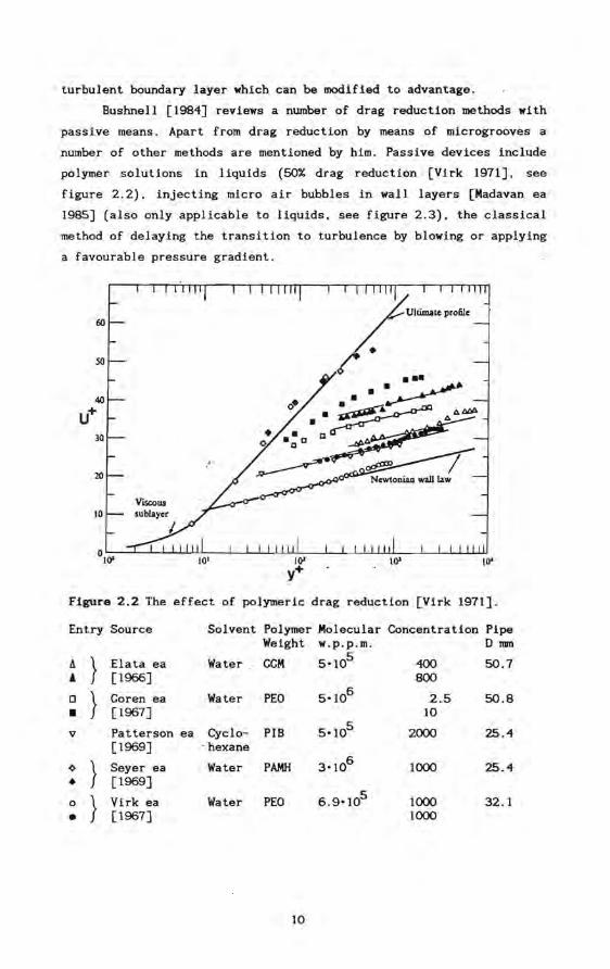
Bushnell [1984] reviews a number of drag reduction methods with

passive means. Apart from drag ' reduction by means of microgrooves a

number of other methods are mentioned by him. Passive devices include

polymer solutions in liquids (50% drag reduction [Virk 1971]. see

figure 2.2). injecting micro air bubbles in wall layers [Madavan ea

1985] (also only applicable to liquids. see figure 2.3). the classical

method of delaying the transition to turbulence by blowing or applying

a favourable pressure gradient.

60 '

50

20

Viscous 10 sublaycr

'-101 10' 10'

Flgure 2.2 The effect of polymeric drag reduction [Virk 1971].

Entry Sou ree Solvent Polymer Molecular Coneentration Pipe Weight w.p.p .m. Dnnn

A } Elata ea Water , GCM 5 0 105 400 50.7 , [l966J BOD

0 } Goren ea Water PEO 5 0 106 2.5 50.8

• [1967J 10

v Patterson ea Cyclo- PIB 5 0 105 2000 25.4 [1969] . hexane

~ } Seyer ea Water PAMH 3 0 106 1000 25.4

• [1969]

0 } Virk ea Water PEO 6.9 0 105 1000 32.1

• [1967J 1000

10

Ij 1.0

iS . 2 0.8

E

:1 0.6

~

<> ~l; ~ Ó ó ~

<> " • ~ "

o i9v~ ~~: <> v .. v ..

:a 0.4 • ] 0.2 •

0.1 0.2 0.3 0.4 O.S 0.6 0 .7

Volumetrie fraclion o( air. QJ(Q. + Q ... )

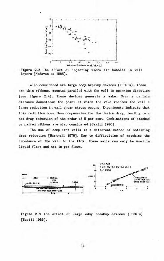
Flgure 2.3 The effect of injecting micro air bubbles in wall layers [Madavan ea 1985J.

Also considered are large eddy breakup devices (LEBU·s). These

are thin ribbons, mounted parallel with the wall in spanwise direction

(see figure 2.4). These devlces generate a wake. Over a certain

distance downstream the point at which the wake reaches the wall a

large reduction in wall shear stress occurs. Experiments indicate that

this reduction more than compensates for the device drag, leading to a

net drag reduction of the order of 5 per cent. Combinations of stacked

or paired ribbons are also considered [Saviii 1986J.

The use of compliant walls is a different method of obtaining

drag reduction [Bushnell 1978J. Due to difficul ties of matching the

impedance of the wall to the flow, these wall scan only be used in

liquld flows and not in gas flows.

t_ ,

O'IATPIATI

OLl"," .... O' • • l1 .. . ,u. "" •• u..0W!_

...

Figure 2.-4 The effect of large eddy breakup devlces (LEBU' s)

[Savl11 1986J .

11

. § 2.2 ldeas and theories concerning drag reduction.

We will now briefly sununarise the classical picture of walls

with surface roughness as provided, for instance, by Schlichting

[1979]. Walls are considered hydrodynamically smooth when the . +

roughness helght does not exceed the viscous sublayer thickness (h < 5). These walls have the smooth wall friction coefficient. A

dimensionless roughness height larger than 70 y+ leads to a completely

rough wall flow. as all of the roughness elements penetrate into the

logarithmic region.

coeff icient.

These walls have an increased friction

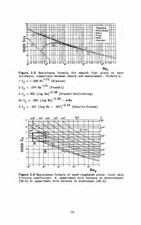
These considerations are derived from drag measurements as

performed by various experimenters. The results are neatly compiled in

figures 2.5 and 2.6 which show the local skin friction coefficient of

a smooth and rough flat surface [Schlichting 1979]. Figure 2.5 shows

the resul ts of drag measurements on a smooth plate compared wi th

several empirical formulas. The scat ter of the experimental data

exceeds 10%, which is an indication of the difficul ties one will

encounter if one wants to establish the 7% drag reduction, obtained by

means of microgrooves. The line 1 describes the friction coefficient

of a laminar boundary layer. Line 3a and the measurements of Kempf

show i ts behaviour during the trans i tion from laminar to turbulent

flow . The other lines and measurements describe tripped boundary

layers which are fully turbulent .

F igure 2.6 shows the local skin friction on a sand-roughened

plate. For a given roughness parameter ks' which is a length

describing the size of the roughness elements. the ratio xIk is s

constant, even if the free stream velocity is changed. So the lines

xlks = const in figure 2.6 describe the skin friction coefficient of a

roughened plate if one varies the free stream velocity above it. Below

a certain velocity the roughness does not lead to an increase in drag

and for high velócities the skin friction coefficient becomes

constant. Also lndicated are the areas (Reynolds numbers and roughness

heights) covered by the present study. The dimensionless roughness . +

heights discussed here are about 10·y in the drag reducing regime,

and fall therefore in the lower end of the transltlon reglon between

12

...

....: U

, , 7 .

i

SI-

~" 1 o

Ol.! o 1 ,..

15

~ . 4

K3 ~.

1 f"'" [\.

'"

1:-- f1eiJSUred 1Jy: • Wieselsberger • Gebers

2 • froude • Kempf .... • Schoenherr

I

14. "'II~

!1 tl ~ ~.

1 V.15 115J • Si 'f)'1S 115J ~ 56 if)1 IS 27SJ • S6 'ti' IS 1151. S6 '11 !5 1153 , S

Rel Flgure 2.5 Resistance formula for smooth flat plate at zero incidence: comparison between theory and measurement. Formula's:

-112 1 Cf 1.328 Re (Blasius)

2 Cf .074 Re-1/5 (Prandtl)

3 Cf 455 (log Re)-2.58 (Prandtl-Schlichting)

-2 58 3a Cf = .455 (log Re) . - AlRe

-264 4 Cf = .427 (log Re - .407) . (Schultz-Grunow)

15

10

_ 5

U o Ol o z.s ,..

lS

~/Xp..

~"z~,

~ ;><.

~

A f--- -

" "" '" Î"-.

"- "" "- "" "-

-.= . - --.. "'-., ~

---. ---. r-- - r--:<~ ~ :::-f- ---. -- ---.

r --B s.;;;;;~~

10' 1 5 10' 1

t;-CQMt

.......

-, -- ----, ----'::: ~

5 'KI' .1

Rex

1

1 rvJ

fw. f'OS 1 2)'/0'

Flgure 2.6 Resistance formula of sand-roughened plate; local skin friction coefficient. A: experiment with balance in waterchannel (§6.6) B: experiment with balance in windtunnel (§6.2).

13

· the smooth wall behaviour and the behaviour at high velocity .

Consequently complex behaviour can be expected. Even anormal sand

roughened plate shows a dip in the value of the skin friction

coeffient in this region. In the case of the microgrooved walls this

dip, apparently, is deep enough to cause some drag reduction.

It is for this reason that classical theories and empirical

relations can not be applied without some reservations. Apart from the

empirical fact that turbulence can be readily influenced no indication

of a potential drag reducing surface could be derived from them.

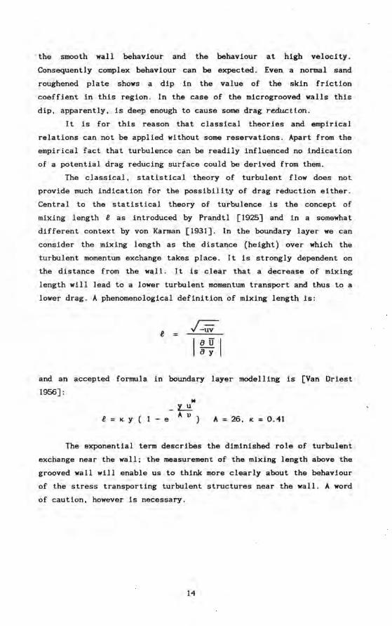
The classical, statistical theory of turbulent flow does not

provide much indication for the possibility of drag reduction either.

Central to the statistical theory of turbulence is the concept of

mixing length ~ as introduced by Prandtl [1925] and in a somewhat

different context by von Karman [1931]. In the boundary layer we can

consider the mixing length as the distance (height) over which the

turbulent momentum exchange takes place. It is strongly dependent on

the distance from the wall. It is clear that a decrease of mixing

length will lead to a lower turbulent momentum transport and thus to a

lower drag. A phenomenological definition of mixing length is:

~ ~

I ~ ~ I and an accepted fonnula in boundary layer modelling is [Van Driest

1956]:

* ~ ~ K Y ( 1 _ e A v ) A 26, K 0.41

rhe exponential term describes the diminished role of turbulent

exchange near the wall; the measurement of the mixing length above the

grooved wall will enable us to think more clearly about the behaviour

of the stress transporting turbulent structures near the wall. A word

of caution, however is necessary.

14

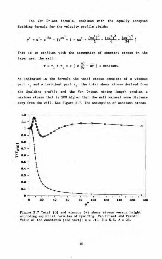
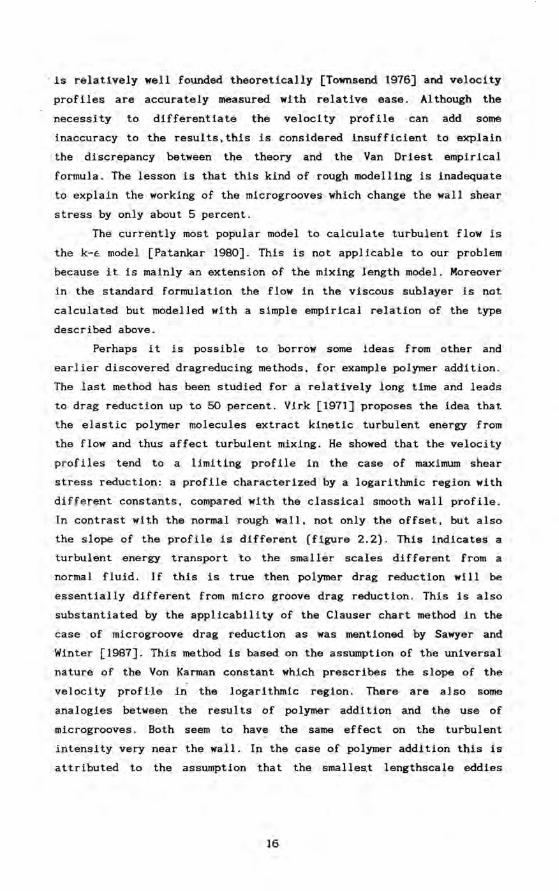
The Van Driest formu!a. combined 'with the equa!!y accepted

Spa!ding formula for the velocity profile yields:

+ 2 + 3 + 4 ~-~-~)

2 6 24

This is in conflict with the assumption of constant stress in the

layer near the wall:

au -p ( v 8y - uv ) constant.

As indicated in the formuia the total stress consists of a viscous

part Tl and a turbulent part Tt' The total shear stress derived from

the Spalding profile and the Van Driest mixing length predict a

maximum stress that is 20% higher than the wall valueat some distance

away from the wall. See figure 2.7. The assumption of constant stress

as ~ ..... ...

1.2

1.1

1

O.G

0.8

0.7

0.8

0.6

0 .•

0.3

0.2

0.1

0 0 20 60 80 100 120 180

y+

Flgure 2.7 Tota! (D) and viscous (+) shear stress versus height according empirica! formulas of Spalding. Van Driest and Prandtl. Va!ue of the constants (see text): K = .41. B = 5.5. A = 26.

15

180

· is relatively weIl founded theoretically [Townsend 1976] and velocity

profiles are accurately rneasured with relative ease. Although the

necessity to differentiate the velocity profile can add sorne

inaccuracy to the results,this is considered insufficient to explain

the discrepancy between the theory and the Van Driest empirical

formula. The lesson is that this kind of rough modelling is inadequate

to explain the working of the microgrooves which change the wall shear

stress by only about 5 percent.

The currently most popular model to calculate turbulent flow is

the k-é model [Patankar 1980]. This is not applicable to our problem

because it is mainly an extension of the mixing length model. Moreover

in the standard formulation the flow in the viscous sublayer is not

calculated but modelled with a simple empirical relation of the type

described above.

Perhaps i t is possible to borrow some ideas from other and

earl ier discovered dragreducing methods, for example polymer addition.

The last method has been studied for a relatively long time and leads

to drag reduction up to 50 percent. Virk [1971] proposes the idea that

the elastic polymer molecules extract kinetic turbulent energy from

the flow and thus affect turbulent mixing. He showed that the velocity

profiles tend to a l1miting profile in the case of maximum shear

stress reduction: a profile characterized by a logarithmic region with

different constants, compared with the classical smooth wall profile.

In contrast wi th the normalrough wal!, not only the offset, but also

the slope of the profile is different (figure 2.2). This indicates a

turbulent energy transport to the smaller scales different from a

normal fluid. If this is true then polymer drag reduction wil 1 be

essentially different from micro groove drag reduction. This is also

substantiated by the applicability of the Clauser chart method in the

case of microgroove drag reduction as was mentioned by Sawyer and

Winter [1987] . This rnethod is based on the assumption of the universa 1

nature of the Von Karman constant which prescribes the slope of the

velocity profi-le in the logarithmlc region. There are also some

analogies between the resul ts of polymer addl tion and the use of

microgrooves. Both seem to have the same effect on the turbulent

intenslty very near thewall. In the case of polymer addition thls Is

attributed to the assumption that the smalles,t lengthscale eddies

16

disappear near the wall thus effectively thickening the viscous

sublayer. This constitutes actually a second idea about the mechanism

of polymer drag reduction.

A test of this idea could he the measurement of accurate spectra

in the viscous sublayer: the higher frequencies should be attenuated.

A second, more indirect way of testing this hypothesis is measuring

the bursting rate near the wal I. A thicker, more stabie viscous

sublayer leads to a lower bursting rate. Ihe lat ter effect has indeed

been observed, both in the case of polymerie drag reduction and micro

groove induced drag reduction.

In this context the surface renewal model of a turbulent

boundary layer should be mentioned [Einstein & L1 1956]. Ihe basic

idea of this model is that the wall layer is periodically replaced by

fluid from the buffer region. This fluid will be slowed down by

viscous forces and forms a new wall layer. Ihis process is described

in the model by a simplified x-momentum equation:

Ut(x, t) ; u Uyy(x, t)

The boundary and initial conditions are:

U(O, t) = 0

U(y, 0) ; Uo ; constant

The solution of this equation is described using the errorfunction:

U( y, t); Uo erf [-y--] J;;;

Z

erf(Z) ~

J e-z2dz

-()Q

The mean wall shear stress and several other quanti ties ' can be

calculated by averaging over one period. One easily obtains the result

that the mean wall shear stress is proportional to the square root of

the time between two renewals (the so called "bursts"), so a 5%

decrease in drag is associated with a 10% decrease in burst frequency,

according to this model.

17

Bechert ea [1986] introduced the term protrusion height of the

riblets. rhey show that the protrusion height by given riblet spacing

is limited. rhe most effective riblets are those with the highest

protrusion helght, because they maximlze the lnfluence on the boundary

layer. rhe optimal spacing of the riblet is derived by the following

argument. lang ea [1984] calculated that the most persistent

perturbation mode in a turbulent boundary layer consists of

longi tudinal counterrotating vortices spaced 90 vlscous units

pairwise. rhe region where the flow has a vertical velocity component

coincides with the position of the observed low speed streaks .

Apparently obstacles interactlng wl th this mode must be spaeed much

less than 45 viscous units, because then every vortex is blocked by

one rib . Bechert also proposes a three dimensional fin instead of an

inf ini te groove ",hich has a much higher protrusion height and must

consequently give a larger .drag reduction.

The calculation of the penetration depth for a longi tudinal

grooveproceeds as follows. For a first approximation we will assurne

the flow independent of the streamwise coordinate x, incompressible,

stationary and with a constant pressure gradient ~. rhe Navier-Stokes

equations reduce to:

v + W 0 Y z

p VU +WU

x (U + Uzz) - -- + v

Y z P yy P

VV +WV - --1-+v (V + Vzz) Y z P yy

P VW +ww z v (W + W ) - --+

Y z P yy zz

Before we proceed, we will normalize the variables on the

* * v P U + u + u p+ = P

x andu + viscous units Y = -v- y, z = -- z, tG v x p * p u u

For convenience we drop the superscripts.

We will not allow secondary flow and so we assurne : V 0 and W

O. rhe equations reduce now to the very simple form :

18

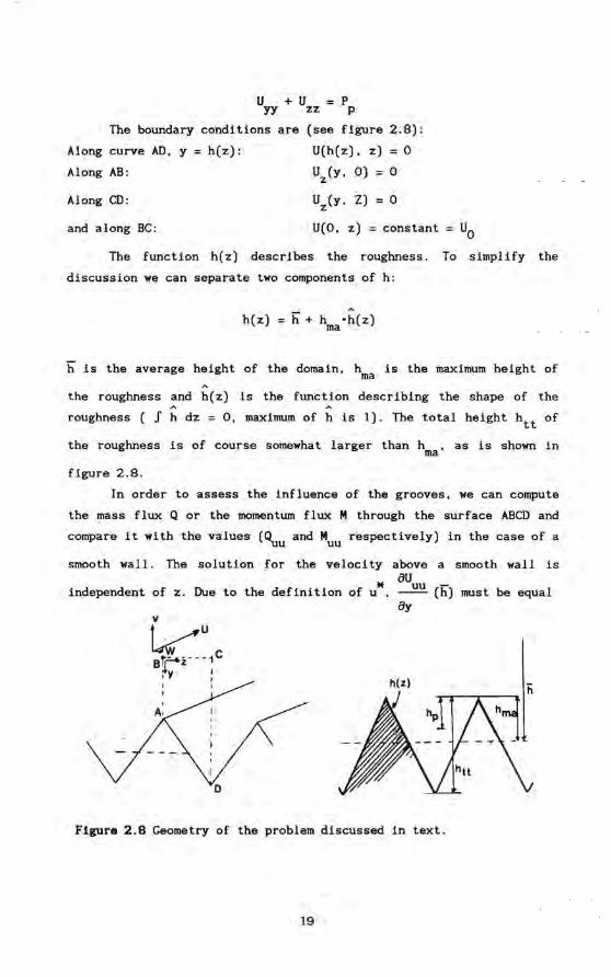
u + u P yy zz p

rhe boundary conditions are (see flgure 2.8):

Along curve AD, y = h(z): U(h(z), z) = 0

Along AB:

Along CD:

and along BC:

Uz(y, 0) = 0

Uz(y, ZJ = 0

U(O, z) = constant = Uo

rhe function h(z) describes the roughness. To simplify the

discussion we can separate two components of h:

A

h(z) = h + hmaoh(z)

h is the ave rage height of the domain, hma is the maximum height of A

the roughness and h(z) is the function describing the shape of the A

roughness ( f h dz = 0, maximum of h is 1). The total height htt of

the roughness is of course somewhat larger than hma , as is shown in

figure 2.8.

In order to assess the influence of the grooves, we can compute

the mass flux Q or the momentum flux M through the surface ABCD and

compare it with the va lues (~u and Muu respectively) in the case of a

smooth wal!. The solution for the velocity above a smooth wal! is au

independent of z. Due to the definition of u*, uu (h) must be equal ay

Figure 2.8 Geometry of the problem discussed in text.

19

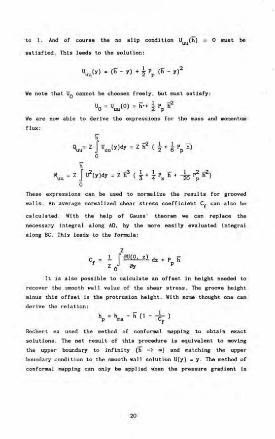
' to 1. And of course the no slip condition u (h) uu

satisfied. This leads to the solution:

u (y) = (h - y) + 1 P (h _ y)2 uu 2 p

We note that Uo cannot be choosen freely, but must satisfy:

- 1 -2 Ua = Uuu(O) = h'+ 2 Pp h

o must be

We are now able to derive the expressions for the mass and momentum

flux:

M uu

h o = z f U (y)dy uu uu

o h

Z h2 ( 1 + 1 P h) 2 6 p

f 2 -a 1 1 - 1 -?-2 = Z U (y)dy = Z h (3 + 4 Px h + 20 r; h )

o These expressions can be used to normal1ze the resul ts for grooved

wal Is. An ave rage normalized shear stress coefficient Cf can also be

calculated. With the help of Gauss' theorem we can replace the

necessary integral along AD, by the more easily evaluated integral

along Be. This leads to the formula:

Z f aU(O,

o ay z) dz + P h

p

It is also possible to calculate an offset in height needed to

recover the smooth wall value of the shear stress. The groove height

minus this offset is the protrusion height. With some thought one can

derive the relation:

h = h - iï (1 __ 1_ ) p ma Cf

Bechert ea used the method of conformal mapping to obtain exact

solutions. The net result of this procedure is equivalent to moving

the upper boundary to infinity (h -) co) and matching the upper

boundary condition to the smooth wall solution U(y) = y. The method of

conformal mapping can only be appl1ed when the pressure gradient is

20

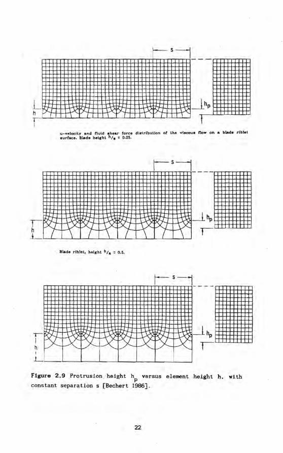
zero. Ooly with special groove geometries one can derive closed

formula for the solution of U and the protrusion height. But the

resul ts indicate that the protrusion height divided by the width of

the grooves tends to a limiting value even if the height of the

grooves is increased (see figure 2.9 for a typical result). Bechert's

resoning does not provide a direct estimate of the amount of drag

reductionwhich can be obtained.

Some other hypothetical mechanisms center around the influence

of the grooves on the observed coherent structures. A possible

mechanism is the resonance with low speed streaks. It is assumed that

coherent structures carry a major part of the momentum transport from

the wall to the flow. A kind of wall attached structure is the low

* * speed streak. Ihis is a long (1000 y ), narrow (lOy ) area where the

veloci ty component in the direction of the free stream is markedly

lower than its ave rage value. These streaks are spaced at 100 viscous

units. As a working hypothesis one could assume that grooves hinder

their formation or decrease their intens i ty if formed. Iwo problems

occur immediately:

I Ihe best dragreducing walls have grooves spaced 20 viscous

uni ts, which seems too narrow for direct interaction wi th those

streaks.

II Even if one sees some influence of the grooves on the streaks,

one still has to prove that the modified streak transports less

momentum.

Apart from performing a visualisation experiment which visualizes all

types of structures, a measurement of the mixing length would yield

some insight whether a turbulent structure whichs transports momentum

near the wall, is affected. A test of the influence of the grooves on

the turbulent structures would be the measurement of the spanwise

correlation of the velocity fluctuations. As normally all near wall

* lengthscales scale on viscous units (v/u ), drag reduction without

change in structures would lead to larger lengthscale and thus to a

broader correlation curve in absolute units. If, loosely speaking, the

grooves somehow cut the structures in pieces thls would lead to a

narrower correlation curve.

And lastly one could suggest that the grooves are able to

suppress the meandering of the low speed steaks.The streaks meander

21

L h r­I

r h L

...;:. r

-Sj -

:). 'I.. J< Y-:. :.x 'I.. J< hp

Î { \ { \ { \ t u-veloctly and nuid .hear force distribution of the vi.eaus flo. on a blad. rtblet. Burf.ce. Blad. hehrht h/B = 0.25.

rf~ Ff ~p;tP(rf~ Blade riblet, helght hl. = 0.5.

r-s~

Figure 2.9 Protrusion height h versus element height h. with . p

constant separation s [Bechert 1986].

22

slowly over the smooth plate. Suppression of this meandering could

reduce the drag (in this case the form drag of the low speed streak to

the rest of the flow). In the extreme case this could be observed as

an attachment of the streak to the grooves. But the two objections of

the former point are still applicable.

§ 2.3 Experimental results from literature concerning drag reduction

with microgrooves.

In the last few years several experiments have been performed

which give information about the nature of the drag reduction attained

with microgrooves.

Reif and Dinkelacker [1982] drew attention to the fact that

sharks and several other fish had smaillongitudinal riblets on their

skin (see figure 2.10).

Liu ea [1966] investigated the effects of small longitudinal

fins on turbulent bursts in the boundary layer. They found a clear

reduction of turbulent burst frequency (figure 2.11) even with a very

wide spacing between the fins (s+ = 100).

Walsh ea [1978] were the first to pay attent ion to microgrooves

in a direct application to drag reduction. They used a dragbalance to

measure the drag directly in a windtunnel at a Reynoldsnumber of about 6 10 . They tested a large number of different grooved walls (see figure

2.12. the best walis). They found a maximum of 7% reduction in drag.

on a grooved plate with a dimensionless groove height h+ of 13 and a

dimensionless width s+of 18. They also observed that the sharpness of

the groove peaks is of importance . Their data imply that the

dimensionless width of the grooves is the proper scaling parameter.

Nitschke [1984] studied the flow in pipes with grooved walis.

The drag was indicated by the pressure drop in a fully developed

turbulent pipe flow. The conclusions were only partly in line with

those of Walsh. She found a maximum drag reduction of about 4% with + + grooves of a height h of 12 and a width s = 10 (figure 2.13).

. + + Reduction occurred in the range of 6 < s < 20. A different groove (s

23

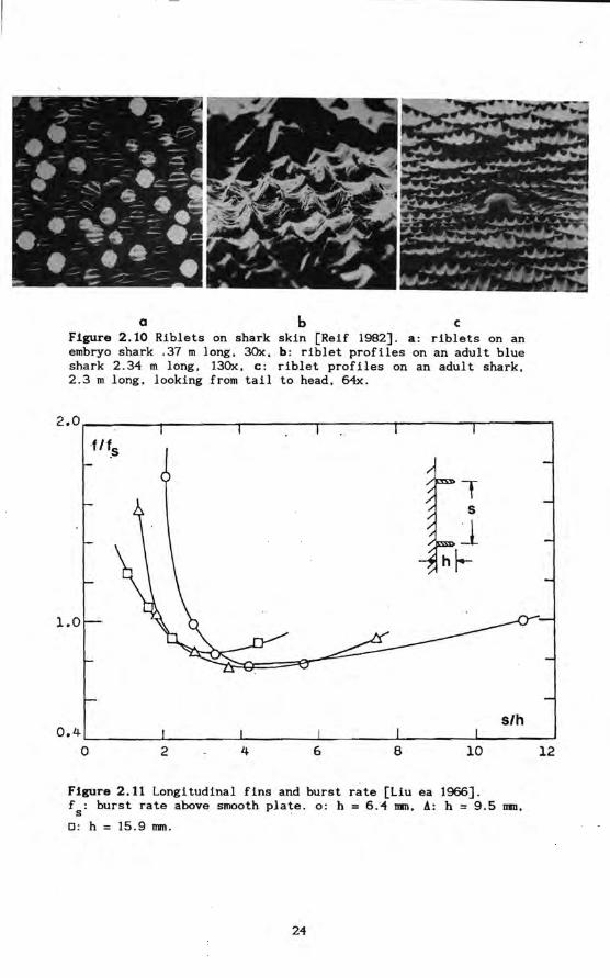
a b c Flgure 2.10 Riblets on shark skin [Reif 1982]. a: riblets on an embryo shark .37 m long. 3Ox. b: riblet profiles on an adult blue shark 2.34 m long, 13Ox, c: riblet profiles on an adult shark, 2.3 m long, looking from tail to head, 64x.

2.0~----~--~---T-------r------ïl------~-----;

1.0

s/h 0.4L-______ ~ ______ ~~ ______ ~ ______ _J ________ ~ ______ _J

o 2 4 6 6 10 12

Flgure 2.11 Longitudinal fins and burst rate [Liu ea 1966]. fs: burst rate above smooth plate. 0: h = 6."1 DIR, A: h = 9.5 DIR.

0: h = 15.9 mmo

2"1

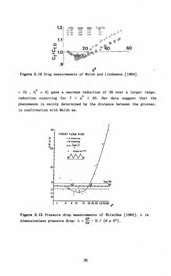
1.2 ~QQlJ. t!l.!!!!!!l. llmi!l!. 1!.~.lt1~:h o UR 0.41 O. dJ II 0 o 1).\\ Q29 0.47 9.l 0 o 7'<\ Q08 " IB 6.1 00

1.1 o 0

§l,j9 00 0

0 ...: 60 ~ 1.0 -0

.9 s+

Figure 2.12 Drag measurements of Walsh and Lindemann [1984].

+ = 15 , h = 4) gave a maximum reduction of 3% over a larger range,

reduction occurring for 1 < s + < 30. Her data suggest that the

phenomenon is mainly determined by the distance between the grooves,

in confirmation with Walsh ea.

30

riblet tube Rl05

~ • À· AnbohNng

.E • e-AnbohlU'lg

~ 6W.~ ~20 ~

.. Q30S.R.-ClZ.

-6

4 6 8 10 15 202530405060 s+

Figure 2.13 Pressure drop measurements of Nitschke [1984], À is

dimensionless pressure drop: À = ~ . D / (~ P U2 ).

25

1.15

1.10

81.05 (,) "-;..1.00 (,)

.95

c c c

c c our data C1:J 0\ ·T·_·--ClQ... ·~' - ,-

~ Walsh '

.'~~ .900!:------=2'="0----,.&'0,...-----='60 s+

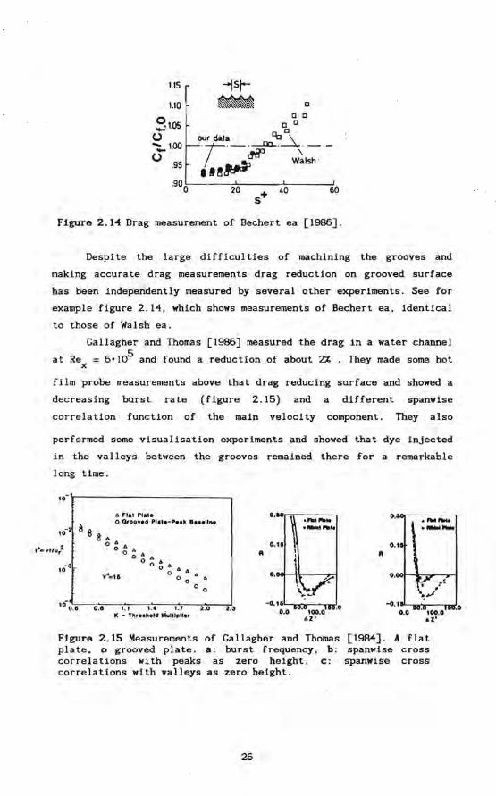
Flgure 2.1~ Drag measurement of Bechert ea [1986].

Despi te the large diff icul ties of machining the grooves and

making accurate drag measurements drag reduction on grooved surface

has been lndependently measured by several other experlments. See for

example figure 2.14, which shows measurements of Bechert ea, ldentical

to those of Walsh ea.

Gallagher and Thomas [1986] measured the drag in a water channel , 5

at Rex = 6'10 and found a reduction of about 2% . They made some hot

film probe measurements above that drag reducing surface and showed a

decreasing burst rate (figure 2 . 15) and a different spanwise

correlation function of the main velocity component. They also

performed some vlsuallsation experiments and showed that dye lnjected

in the valleys between the grooves remalned there for a remarkable

long time.

10-r----------------------------,

lÖO,5

6 Flat Plat. Q O,ooved Pla.a-P •• k a ••• IIIM

88 8 .. o g A 4

o .. o 0 ~ b-

o ~ .6. b. .6-

00 ..

00

0.. 1. 1 1.4 1.1 2.0 IC - Thr •• hold MulUpU.r

2.3

o.aor---.-:_--..... -1 ._-

0.'8 A A

Flgure 2.15 Measurements of Gallagher and Thomas [19B~]. A flat plate, 0 grooved plate. a: burst frequency, b: spanwlse cross correlations with peaks as zero helght, c: spanwise cross correlations with valleys as zero height .

26

Sawyer and Winter [1987] performed a set of careful windtunnel

measurements with a dragbalance and hot wire probe. They confirmed the

results of Walsh ea in details. The changes in thelogarithmic region

of the velocity profiles due to the different surfaces confirmed their

balance measurements.

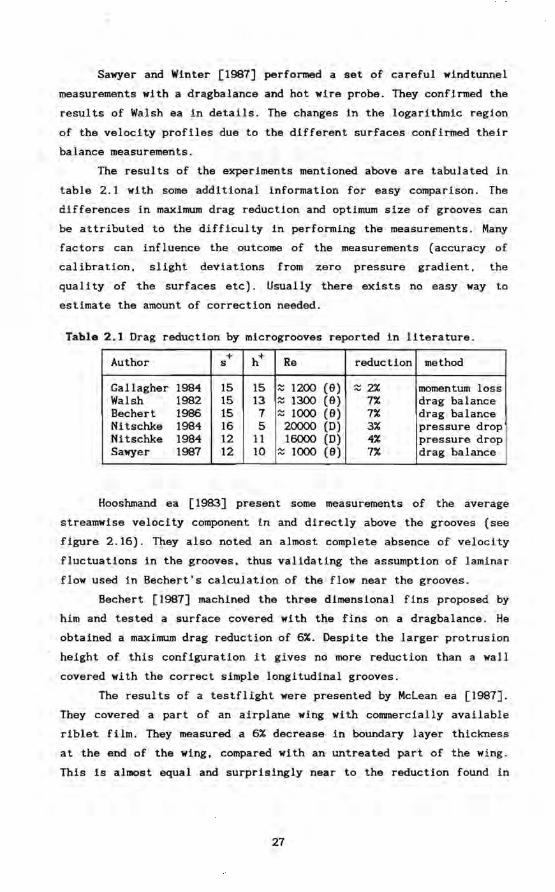
The results of the experiments mentioned above are tabulated in

table 2.1 with some addi tional information for easy comparison. The

differences in maximum drag reduction and optimum size of grooves can

be attributed to the difficul ty in performing the measurements. Many

factors can influence the outcome of the measurements (accuracy of

calibration, slight deviations from zero pressure gradient, the

qua 1 i ty of the surfaces etc). Usually there exists no easy way to

estimate the amount of correction needed.

Tabla 2.1 Drag reduction by microgrooves reported in literature.

Author + h+ Re reduction method s

Gallagher 1984 15 15 -1200 (9) :::: 2% momentum loss -Walsh 1982 15 13 :::: 1300 (9) 7% drag balance Bechert 1986 15 7 :::: 1000 (9) 7% drag balance Nitschke 1984 16 5 20000 (0) 3% pressure drop Nitschke 1984 12 11 16000 (0) 4% pressure drop Sawyer 1987 12 10 :::: 1000 (9) 7% drag balance

Hooshmand ea [1983] present some measurements of the ave rage

streamwise velocity component in and directly above the grooves (see

figure 2.16). They also noted an almost complete absence of velocity

fluctuations in the grooves, thus validating the assumption of laminar

flow used in Bechert's calculation of the flow near the grooves.

Bechert [1987] machined the three dimensional fins proposed by

him and tested a surface covered with the fins on a dragbalance. He

obtained a maximum drag reduction of 6% . Despite the larger protrusion

height of this configuration it gives no more reduction than a wall

covered with the correct simple longitudinal grooves.

The results of a testflight were presented by McLean ea [1987J.

They covered a part of an airplane wing with convnercially available

riblet film. They measured a 6% decrease in boundary layer thickness

at the end of the wing, compared with an untreated part of the wing.

This is almost equal and surprisingly near to the reduction found in

27

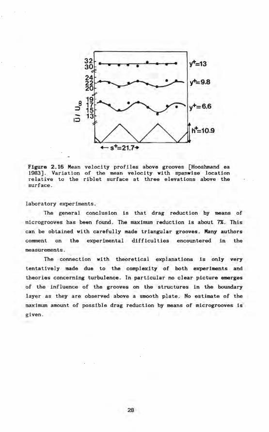
• • •• • • • • • y+=13

-I~

Figure 2.16 Mean veloei ty proflles above grooves [Hooshmand ea 1983]. Variation of the mean veloeity with spanwise loeation relative to the riblet surfaee at three elevations above the surfaee.

laboratory experiments.

The general eonelusion Is that drag reduetion by means of

microgrooves has been found. The maximum reduction is about 7%. This

can be obtained with carefully made triangular grooves. Many authors

comment on the experimental difficul ties encountered in the

measurements.

The eonnection with theoretical explanations is only very

tentatively made due to the complexity of both experiments and

theories concerning turbulence. In particular no clear picture emerges

of the influence of the grooves on the structures in the boundary

layer as they are observed· above a smooth plate. No estimate of the

maximum amount of possible drag reduction by means of microgrooves is

given.

28

Chapter 3 Experimental set-up.

§ 3.1 Waterchannel.

Most of the data presented in this thesis were obtained from

experiments in a water channel available in the Laboratory for Fluid

Dynamics and Heat Transfer at Eindhoven Universi ty of Techno 1 ogy .

Because of the relatively large turbulent lengthscales and low

frequencies in a low speed water channel, detailed studies of the

turbulent flow near the wall are possible by using laser doppler

anemometry and flow visualisation.

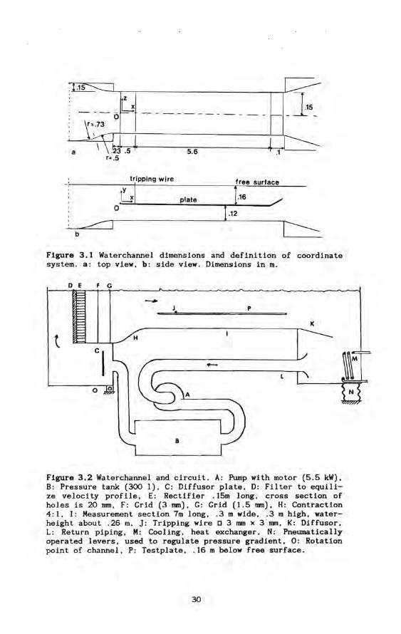
The main dimensions of the water channel are presented in figure

3.1. The measurement section is .3 m wi4e, .3 m high and 7 m long. A

simplified scheme of the water channel is presented in figure 3.2.

Considerable care was taken to have a lew turbulent mean flow and 'a

uniform velocity profile at the entrance. To obtain this the original

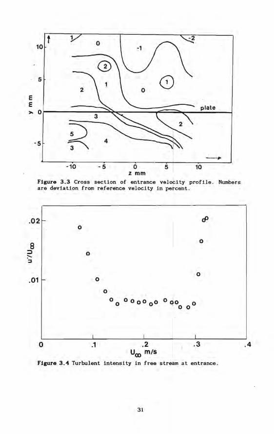
contraction was improved and rebuilt. The lateral cross section of the

velocity profile is shown in figure 3.3. Data on the turbulent

intensity in the free stream are presented in figure 3.4. It shows

that the turbulent intensity at the ent rance of the measurement

sectlon is .6%. The increase in turbulent intensity below .1 mis is

partly due to an instrumental error, the increase at veloeities higher

than .3 mis is caused by cavitation at same abrupt edges in the return

pipes. Presumably due to interaction between the boundary layers and

the free stream, the turbulent intensity increases downstream to a

value of 1.5% at the lower speed and to .8% at a speed of .3 mis.

The free stream speed can he adjusted from almost zero to .4

mis. The highest Reynolds numbers are obtained at the end of the 7 m

long measurement section: Rex = 2'106 and Ree ~ 3000

All measurements are performed on a flat plate mounted as a

false floor at ca 160 rmn below the water surface. The part of the

plate upstream of theroughness elements (described in §3.3) consists

of very smooth glass surfaces of 2 m long and .3 m wide. The leading

edge is . sharpened to provide a start of the· boundary layer without

separation effects. At .7 m downstream of the edge a tripping wire of

3 x 3 1IIIl2 square cross section is placed on the plate and the

29

5.6 .1

tripping wlre tree sLirtace

I~I plate 1.16 /' o==~----~~--~I~·12~---

1-------Flgure 3.1 Waterchannel dimensions and deflnition of coordinate system. a: top view. b: side view. Dimensions in m.

OEF G

- J p . K

t H

-L

o A

Flgure 3.2 Waterchannel and circuit. A: Pump with motor (5.5 kW). B: Pressure tank (300 1). C: Diffusor plate. D: Filter to equili­ze velocity profile. E: Rectifier .15m long. cross section of holes is 20 mmo F: Grid (3 mm). G: Grid (1.5 mm). H: Contraction 4:1. I: Measurement section 7m long .. 3 m wide •. 3 m high. water­height about .26 m. J: Tripping wire 0 3 mm x 3°mm. K: Diffusor. L: Return piping. M:Cool1ng. heat exchanger. N: Pneumatically operated levers. used to regulate pressure gradient. 0: Rotation point of channel. P: Testplate .. 16 m below free surface.

30

1 t -2 o 10 -1

5

E

~ 0~---=::~~~-2~==~~::~~~-J

-5

Flgure 3.3 Cross section of ent rance veloçity profile. Numbers are devlation from reference velocity in percent .

. 021-o

o

.01 I- o

o

I

o .1

o

o

00 0 00000 0 ~oo 00

I I

.2 Uw mIs

.3

Flgure3.4 Turbulent intensity in free stream at entrance.

31

.4

6

u-o 5 o o

4

1 2

---__ b ---------a

3 4 5

x .m

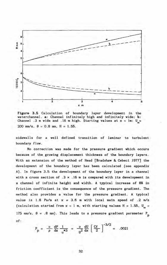
Flgure 3.5 Calculation of boundary layer development in the waterchannel. a: Channel infinitely high and infinitely wide; b: Channel .3 m wide and .16 m high . Starting values at x = 1m: Uoo= 200 mm/s. e = 0.8 mmo H = 1.55.

sidewalls for a weIl deflned transition of laminar to turbulent

boundary flow.

No correction was made for the pressure gradient which occurs

because of the .growing displacement thickness of the boundary layers ;

With an extension of the method of Head [Bradshaw & Cebeci 1977] the

development of the boundary layer has been calculated (see appendix

A). In figure 3.5 the development of the boundary layer in a channel

with a cross section of .3 x .16 m is compared with its development in

a channel of infinite height and width. A typlcal lncrease of 8% in

friction coefficlent is the consequence of the pressure gradient. The

method also provides a value for the pressure gradient. A typical

value is 1.8 Pa/m at x = 3.6 m with local maln speed of .2 m/s

(calculation started ' from x = 1 m. with starting values H = 1.55. Um

175 mm/s. e = .8 mm). This leads to a pressure gradient parameter P

of:

p . p

v dP 1 pdx lE3

u .0021

32

p

Measurements with the LDA at this Positibn indicated a pressure

gradient of 1.8 ± .2 Palm. Although not zero Ithls is still a low value

and as we are interested in near wall pheno~na whlch are relatively

insensitive to pressure gradient. correctivEi actions were considered

not necessary.

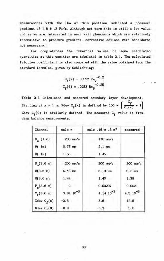
For completeness the numerical values of some calculated

quantities at this position are tabulated in table 3.1. The calculated

friction coefficient is also compared with the value obtained from the

standard formulas. given by Schlichting:

Tabla 3.1 Calculated and measured boundar\Y layer development.

Starting at x = 1 m. %dey Cf(x) is defined i:Jy 100 * [ Cf~~) - 1]

%dey Cf (9) is similarly defined. The measured Cf value is from

drag balance measurements .

Channel calc (I) calc . 16 1x .3 m2 measured

U (1 m) 200 nrnIs 176 nun/s (I)

9( 1m) 0.75 mm 2.1 mm

H( 1m) 1.55 1.45

U(I)(3.6 m) 200 nun/s 200 nun/s 200 nun/s

9(3.6 m) 6.45 mm 6 . 19 mm 6.2 mm I

H(3.6 m) 1.44 . I

1.10 1.39

P (3.6 m) 0 0.90207 0.0021 P

Cf C3.6m) 3.84 10-3 4' 14 10-3 4.5 10-3

%dey CfCx) -3.5 3.6 12.8

%dey Cf (9) -8 . 9 -3 . 2 5.6

33

§ 3.2 Measurement system.

The measurements in a water channel can take a long time. due to

the large timescales involved. Iypical values of v and u* are 10-6

m2 /s and .01 rn/s respectively. Ihis leads to a timescale of .01 sec.

In a windtunnel typical values of v and u* are 15.10-6 m2 /s and .5 rn/s

respectively. which leads to a t * of 60 JlS. Roughly two orders of

magnitude smaller! Measuring a velocity profile with reasonable

accuracy. for instance. takes at least 5 hours in the water channel

(10 minutes averaging time for every of the 30 points). while in the

windtunnel i t could be done in 2 minutes. Ihis difference in time

scales makes the use of automatic datalogging equipment almost

mandat~ry. In the present operational system only an occasional

inspection during the 5 hours is necessary for this kind of

measurement.

Ihe measurement system is built around a PDP 11-23 minicomputer.

with 256 Kbyte memory. two dual density S" diskdrives (type RX02). a

VTI25 graphics terminal and a 20 Mb Winches ter diskdrive. Ihe

operating system used is RIll-VS, the standard system in use for

PDP-11 computers.

Although a Fortran and a C compiler is available. most programs

are written in PEP, an Algol-like language. Because PEP is normally

used as an interpreter, program development is very fast. For faster

execution a compiler can he used and the fastest execution is obtained

by linking handwritten assembly subroutines with the interpreter. For

most applications the interpreter is fast enough, only the sampling

programs have been written in assembly language.

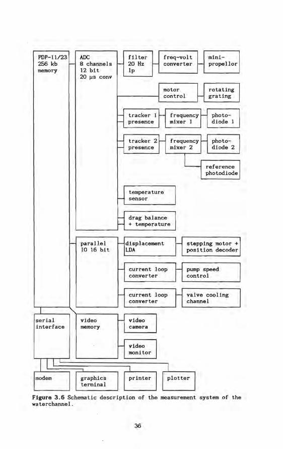
In figure 3.6 aschematic description of the complete

measurement system is given. We will nowmake a few cornments on the

different subsystems.

Ihe minipropellor is an instrument to measure waterveloei ty

developed by the Delft Hydraulics Laboratory. It is used mainly to

moni tor the free stream, downstream of the LDA and visualisation·

experiment. lts measurement area is about 4 cm2 •

rhe temperature meter measures the watertemperature of the

channel. Accuracy is .1 °c, and stabi.1ity better than .01 °C. lts

reading is used to regulate the valve of the cooling spiral.

34

The LDA system is decribed in more detail in Kern [1984]. We I

point out some important details. The rotatin~ grating (purchased from

TPD, Delft) is needed to provide a preshift lfreqUency of 810 kHz in

the laserbeams of the LDA. It consists of la radial and concentric

grating. These produce nine laserbeams of whith three are used for the

measurement of two velocity components in the channel in the reference

beam mode. Two other beams are used to measure the introduced

preshift. The mixing circuit is used to subtqact the frequency of the

signal from the reference diode from the freduency of the signal from

photodiodes 1 and 2. In a second set of mixers a crystal stabilized

frequency of 217 kHz is added to the signals. The frequencies are

converted to slowly varying oe signal by Disa type 55N21 frequency

trackers. Only the range 33-330 kHz is used. !Output filt.ers limit the

response time of the . trackers equivalent to ~ 60 Hz, first order, low

pass filter . Measured spectra show that the 'amount of high frequency

information lost is negligible up to the maximum flow speed used ( . 3

mis) .

The displacement system allows a vertical translation of the LOA

over a distance of 120 DUn,

makes possible the automatic

The centrifugal pump

elecironically stabilised ac

with a resolutif' n of a few microns. It

measurement of a velocity profile.

of the waterc~annel .Is driven by an

motor . The pump I spèed can be controlled

manually or with a 20mA current loop input driven by the computer.

The picture digitizer is a plug-in unit for the PDP-II computer.

I t consists of the circuitboards QRGB-256 a~d QFG-01, purchased from

Matrox. The camera is a Philips black white CCD camera. The

videorecorder and monitor are standard HVS colour video equipment.

The electronics of the drag balance were developed together with

the balance i tself (Chapter 6). The drag baiLance output is a single

analog low frequency signal, -IOVto +10V. !

The modem is used to transfer data to 0f her computers.

35

PDP-l1/23 ADC filter freq-volt mini-256 kb f- 8 channels r- 20 Hz r- converter "- propellor memory 12 bit lp

20 I-LS conv

motor rotating

L control grating

H tracker 1 frequency photo-presence mixer 1 diode 1

H tracker 2 frequency photo-presence mixer 2 diode 2

~ ,e'e,ence photodiode

H tempera ture sensor I

~ drag balance I + temperature

f- parallel HdisPlacement stepping motor +1 10 16 bit LDA posi tion decoder

M current loop pump speed

I converter control

H

current loop valve cooling converter channel

I ser ia 1 video H video

I interface memory camera

f- video I monitor

I I I I I modem graphics printer I I plotter I

terminal

Figure 3.6 Schematic description of the measurement system of the waterchannel.

36

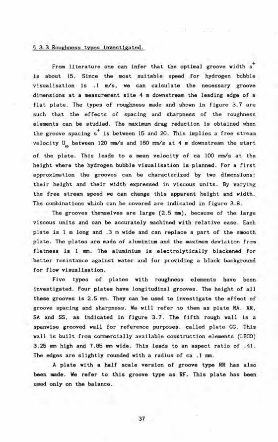
§ 3.3 Roughness types investigated .

From 11 terature one can infer that thei optima1 groove width s +

is about 15. Since the most suitable speed for hydrogen bubble

visualisation is .1 mis, we can calculatethe necessary groove

dimensions at a measurement site 4 m downstr~am the leading edge of a

flat plate. The types of roughness made and l shown in figure 3.7 are

such that the effects of spacing and sha):"pness of the roughness

elements can he studied. The maximum drag reduction is obtained when

the groove spacing s+ is between 15 and 20. Ihis implies a free stream

velocity Uro between 120 mm/s and 160 mm/s at 4 m downstream the start

of the plate. This leads to a mean velocity of ca 100 mm/s at the

height where the hydrogen bubble visualisatior. is planned. For a first

approximation the grooves can he characterlized by two dimensions: 1

their height and their width expressed in viscous units. By varying

the free stream speed we can change this apparent height and width.

The combinations which can he covered are ind~cated in figure 3.8.

The grooves themselves are large (2.5 ~), because of the large

viscous units and can be accurately machined with relative ease. Each

plate is 1 m long and .3 m wide and can replace a part of the smooth

plate. The plates are made of aluminium and the maximum deviation from

flatness is 1 mm . The aluminium is electrolytically blackened for

bet ter resistance against water and for pro, iding a black background

for flow visualisation.

Five types of plates

investigated. Four plates have

with roughnJ ss elements have been

longitudinal g~ooves. The height of all

these grooves is 2.5 mm. They can be used to investigate the effect of

groove spacing and sharpness. We will refer to them as plate RA, RR,

SA and SS, as indicated in figure 3.7. Tha fifth rough wall is a

spanwise grooved wall for reference purpose$, . called plate CG. This

wall is built from commercially available construction elements (LEGO)

3.25 mm high and 7.85 mm wide. This leads to an aspect ratio of .41.

The edges are slightly rounded with a radius of ca .1 mm.

A plate w!th a half scale version of I groove type RR

been made. We refer to this groove type as RF. This pla te

used only on the balance.

37

has also

has been

~l ~I 2.5 2.5

~I ~l 5.0 5.0

2.5

~ll GG • •

15.7

Flgure 3.7 Geometry and nomenclature of grooves.

50r---------------------------------------------,

reduct ion , '

20 40 60 80 s· '

Flgute 3.8 Groove geometries in relation to estimated area of dragreduction.

38

, I .

;:!!!illlllll!lllmrrmlllllllllllrll uu

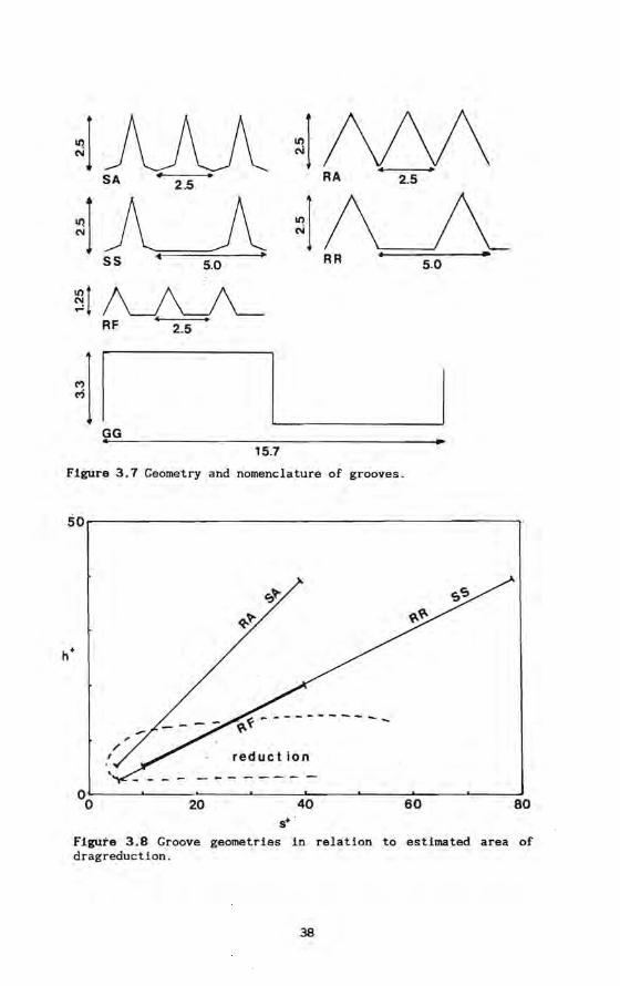
Fl~re 3.9 Iso-velocity contours abovedifferent grooves. Protrusion height h is indicated.

p

39

In order to get an idea about the behaviour of the plates we

applied the calculation of Bechert to these surfaces . Because the

analytical solutions obtained by Bechert are only sui ted to very

special shapes of roughness. we resorted to numerical methods.

Two different methods lead to a numerical approximation of his

equations. First we can write down a general solution to the eq~tion

v2 U = P on the domain ABCD as decribed in figure 2.9. satisfying the x

boundary conditions at the top and sides of the domain :

Q)

U( y. z) 1 2 \: [n 1T z]. [~] Uo + AoY + 2 P~ + L Ancos ---z--- Slnh Z

n=l

The constants An need to be determined by applying the remaining

boundary condition along AD (figure 2.9). An advantage of this method

is that AO is directly proportional to the friction coefficient. This

is. however. not the most accurate way to obtain a solution due to

problems with numerical stability.

It is more convenient to solve the differential equation

directly which leads to the second method and which we used in the

resul ts presented here. The solution can be obtained by standard

numerical methods like discretizing the equation on a fine grid and

solving the resulting linear matrix equation iteratively with a

Gauss-Seidel method. The solutions presented here were obtained on a

grid of 41 x 91 points. Convergence tests from coarser grids enables

us to estimate that the solution approximates the exact solution

within 1%.

A graphical view of the solutions is shown in figure 3.9. The

lines are iso-veloci ty contours . They give an indication to which

height the flow is influenced by the presence of the ' grooves.

In table 3.2 the results of these calculations are compiled. For

a description of the symbols we refer to figure 2.8. The vertical

dimension of the domains is chosen such that h = 20. The pressure

gradient parameter Pp was zero. Cf is the viscous drag normalized with

the smooth wall value.S is the relative surface area of the grooves.

As can be seen from figure 2.8 htt is tQe roughness height from top to

40

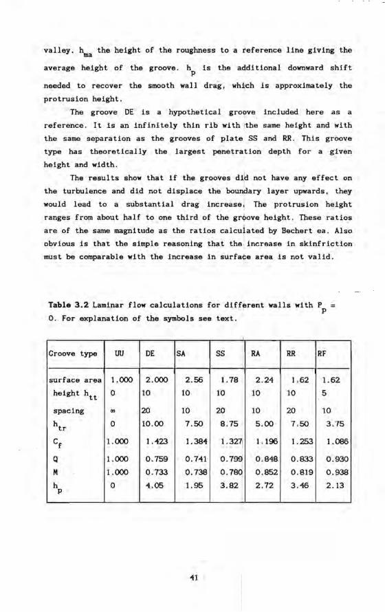
valley, hma the helght of the roughness to a teference llne glvlng the

ave rage helght of the groove. h is the addi tional downward shift p I

needed to recover the smooth walldrag, wh~ch is approximately the

protrusion height.

The groove DE is a hypothetical groQve included here as a

reference . It is an infinitely thin rib with Ithe same height and with I .

the same separation as the grooves of plate : SS and RR. This groove

type has theoretically the largest penetration depth for a given

height and width.

The results show that if the grooves di~ not have any effect on

the turbulence and did not dlsplace the bounbary layer upwards, they

would lead to a substantial drag increasel The protrusion height

ranges from about half to one third of the gr ove height. These ratios

are of the same magnitude as the ratlos calcu ated by Bechert ea. Also

obvious is that the simple reasoning that the 1increase in skinfriction

must be comparable with the increase in surfaf e area is not valid.

Tabla 3.2 Lamlnar flow calculatlons for dlff~rent walls wlth P = I p

O. For explanation of the symbols see text.

Groove type UU DE SA SS I

RA RR RF

surf ace area 1.000 2.000 2.56 1. 78 1

2.24 1.62 1.62

height htt 0 10 10 10 10 10 5

spacing 00 20 10 20 10 20 10

htr 0 10.00 7.50 8:75 5.00 7.50 3.75

Cf 1.000 1.423 1.384 1. 3271 1.196 1.253 1.086

Q 1.000 0.759 0.741 0.799 ·0.848. 0.833 0.930

M 1.000 0.733 0.738 0.780 0.852 0.819 0.938

h 0 4.05 L95 3.82 2.72 3.46 2.13 p

41

· Chapter 4 Single point measurements.

§ 4.1 Introduction.

Although several publications present single point measurements

above grooved surfaces (see §2.3) 'some worthwhile additions can be

made to them. Most measurements, wi th the exception of Wallace ea

[1983], were done at relatively large Reynolds numbers and wi th hot

wire or filmprobes whose dimensions are at least ten viscous units.

The measurement volume of the LDA at our disposal is less than one

viscous unit high and less than 5 units long, which adds to the

reliabi 11 ty of the resul ts. Another advantage is tha t with the LDA it

is possible to measure simul Ümeously two velocity components exactly

at the same position. It is for this reason that measurements of

higher order moments obtained with multiwire probes, especially cross

correlations between different velocity components are relatively

unreliable. Measurement of the vertical velocity component very close

to the wall are virtually impossible with hotwire probes.

Therefore .our attention has focused on the near wall measurement

of two velocity components wi th the LDA . From other publications it

appears that the influence of the grooves on the mean velocity profile

is only minor, and so the natural question is whether the higher order

moments are equally unaffected and if they are affected what its

significance is. For example: it is argued bysome [Gallagher 1984]

that a change in third order quantities likeskewness ( \? ) indicate

a change in turbulent burst frequency. Also in turbulent modelling it

is generally assumed that the intensity of turbulent fluctuations is

. proportional to the shear stress.

As has been noted in §3.2 water channelpoint measurements are

not especially suited to obtain accurate data due to the long

timescales involved. Still the measurements with a LDA have the merit

that they are obtained with a very stabie apparatus which does not

require extensive calibration and which has a small measurement volume

in relation to the viscous lengthscales.

To the best of the author's knowledge only Djenidi ea [1987]

have done similar detailed measurements above grooved surfaces. They

present only velocity profiles and second order quantities u' and v'.

42

I In order to compensate some of the disadvantages of LDA a few

measurements were also performed in a windtunnel of the Delft

University of Technology . Those data were obtained with hot wire

anemometry.

§ 4.2 Profiles.

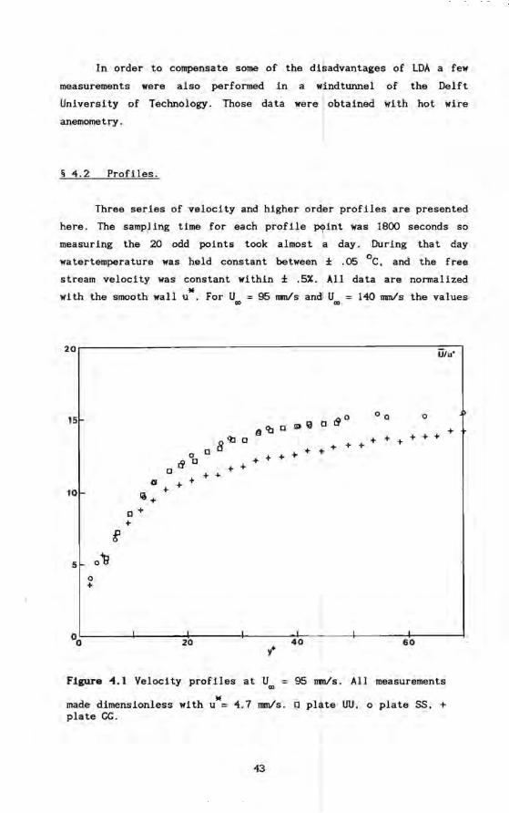
Three series of velocity and higher order profiles are presented

here . The sampling time for each profile 1 int was 1BOO seconds so

measuring the 20 odd points took almost a day. During that day

watertemperature was held constant between ± .05 oe. and the free

stream velocity was constant within ± .5%. I All data are normalized

with the smooth wall uw . For U = 95 mm/s andl U = 140 mm/s the va lues a> a>

2or---------------------------------------------------~~~ U/u'

lS

10

S

o +

o-te

8 <b c o 0

{j C + + C + ...

Cl + + +

Iè+

C + +

a <à C

+ + +

I {jo 00 0

IlJIEJ C +

+ + + + + + + + +

+ + +

°0L-------~-------2~0~------4--------4~0~-4----~------~6~O-------4 y+

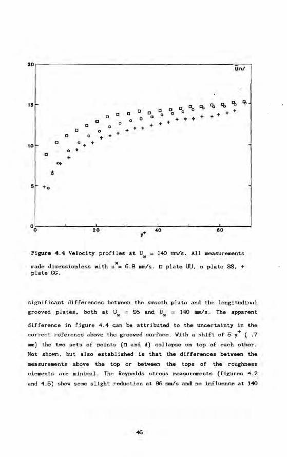
Figure ~.1 Velocity profiles at Ua> = 95 mmls . All measurements

made dimensionless with u*= 4.7 mm/s. D PIt te UU. 0 plate SS. + plate CG.

43

3

+ 2

0 0

+0

00

0

o I--'-----L + + + ++

.8

.6

.4

+ +

+

of------../

.8

.6

.4

+ .2 0 8

o a +

o

+ + + + + + + + + + + + + V'Af ++ + +

+

00 o o

+ + + + + + + + o

o o o

-UV/~

oL--~--~--~-~--~--~-~~-~ o 20 + 40 60

Y

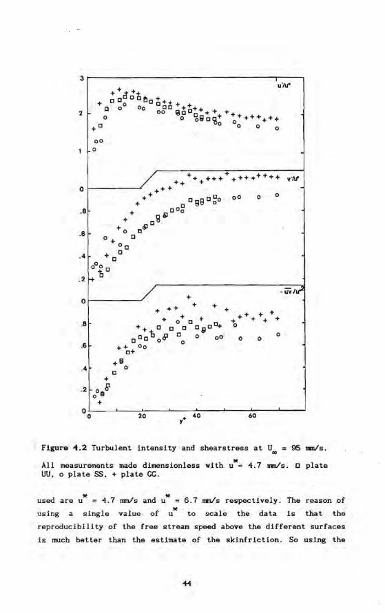
Figure ~.2 Turbulent intensity and shearstress at U~ = 95 mmls .

All measurements made dimensionless with u*= 4.7 mmls. 0 plate UU, 0 plate SS, + plate CG.

*. * used are u = 4.7 mmls and u 6.7 mm/s respectively. Tbe reason of

u* . to scale the data is that the using a single value of

reproducibility of the free stream speed above the different surfaces

is much better than the estlmate of the skinfrictlon. So using the

0.5

o

-,5 5

o

-.5 .5

o

-.5 .5

o

+0 0 I

- 0 :UJlIt"J .

0 0 +

+ 0 0 ++

[,.p°0 1, + .p 0+ t t/$ :t" ~ + + ~ + -bot: + + + + 0

00 -to O . 0 0 o . Cl o 0

00 uui/u'J

0000 + ~~ 8~.p~9 + -.of ~$ + ~~ + +~+ + ~

+.p 0;' + + .+ OV I + 00 I

~ ,

0

gl:S uVV/U',J 0

+ .IJ + 0

tlO

0

0 0

0 0 +

""

+

+

+

ct] 0~·~'b.p0 + . O+Jtr~~B \O+-tot++.+++

o 0 + 0

V3/U'"

o 0+ otl+++1;~+ +++ +~

D+ + ~ 00 0 n + ... -ti +,:!l []

o c +u Cl., e-r

+ o 0

20 ,.. 40 Y

60

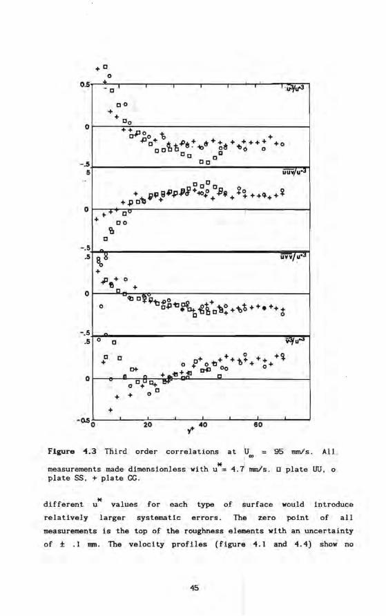
Flgure 4.3 Third order correlations at foo = 95 mm1s. All

. * ' measurements made dimensionless with u = 4.7 mm1s. 0 plate UU,o plate SS, + plate CG.

different * uvalues for each type of surface would introduce

relatively larger systematic errors. Tha zero point of all

measurements is the top of the roughness elements with an uncertainty

of ± .1 II'1II. The velocity proflles (figure 4.1 and 4.4) show no

45

I

2or-----------------------------------------------------~~_, Ü/u·

15 c c c

c c 0 c 0 0 C 0

C 0 + + 0 + + C 0 + C 0 + +

+ 10

c 0+ +

0 + C

+ 0+

~

5 +0

°0~------4-------~2~~------~--------4~0--~--~------~6~O~----~ y+

Flgure 4.4 Velocity profiles at U = 140 mm1s. All measurements '"

made dimensionless with u*= 6.B mm1s. 0 plate UU, 0 plate SS, + plate CG.

significant differences between the smooth plate and the longitudinal

grooved plates, both at U.,;, = 95 and U", = 140 mm/s. rhe apparent

difference in figure 4.4 can be attributed to the uncertainty in the

correct reference above the grooved surface. With a shift of 5 y+ ( .7

mm) the two sets of points (0 and A) collapse on top of each other.

Not shown, but also established is that the differences between the

measurements above the top or between the tops of the roughness

elements are minimal. rhe Reynolds stress measurements (figures 4.2

and 4.5) show some slight reduction at 96 mm/s and no influence at 140

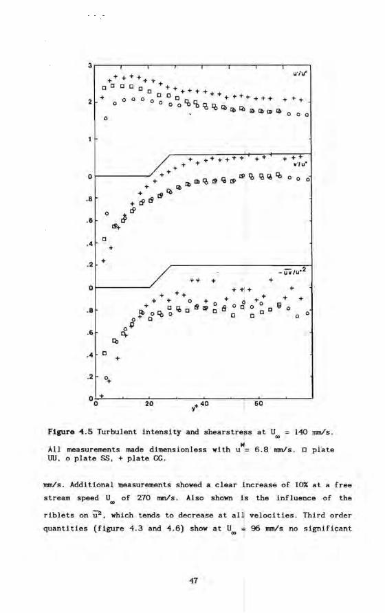
[J .4

+

.2 +

++ 0

+ ++ + + 0 +

Qj+ [J1è[J~1lP .8 + 0 ~ 0 o [J

.6 0+1 '+

Cb

.4 [J +

.2 0+

00 +

20 ot 40 Y .

+

+ 0 a [J

I + + + + +

v1u·

lölè~ooo

+ + +1 + , + o [Jo +0

o C [J [J [J

60

+ + +

lil 0

o 0

Flgure 4.5 Turbulent intenslty and shearstre~s at Um = 140 mm/s.

All measurements made dlmensionless with u1= 6.8 mm/s . D plate UU, 0 plate SS, + plateCC.

mm/s. Additional measurements showed a clear increase of 10% at a free

stream speed Um of 270 mm/s. Also shown 1s the influence of the

rib.1ets on \ï2, which tends to decrease at al~ velocities . Third order

quantities (figure 4.3 and 4.6) show at Um ~ 96 mm/s no significant

47

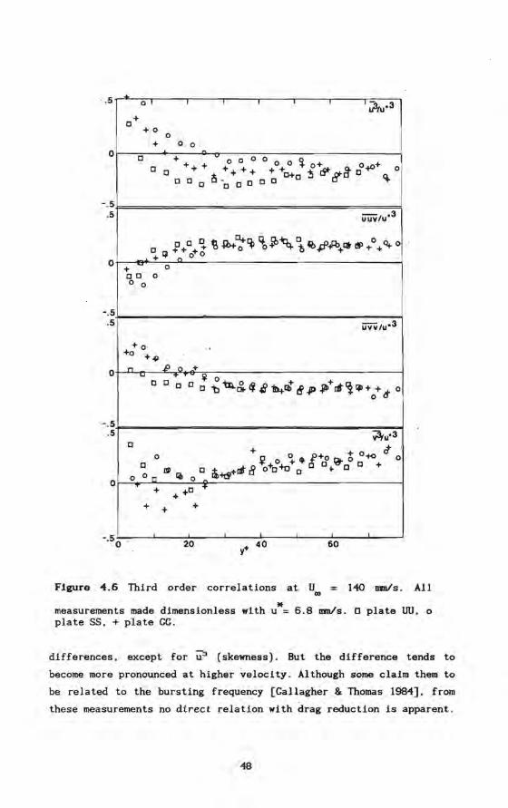
· .5

o

-.5 .5

o

-.5 .5

o

-.5 .5

o

0 J3tu· 3 + [J

+0 0

+ o 0

[J + + voo 0 0 0 0 ~ 0+ 0 + [J [J ++

+ + + + + +CJ+ :!i ó* rr8' a -tO 0 a a [J iS '[J [J [J [J [J a ~

üüV/u·3

[J ~+[J + ~ fO ~~~ %~~ t 4b#fb+~ lil +0 + ~ 0 + ~ 0 0 0 .

+ 0 [J[J 0 o 0

UvY/u·3

+0 +0 +-9

n .iJ 0 +

ua[J ~°"tJ4.0 + + [J a [J ti G ~ Ii ~Iai ti.JP ~ alt ~ ~ + 0+ d' 0

[J

0 [J ~ [J

0 o Cl Ii 0

+ +[J ... +

+ + +

20

;3,u·3

+ + 0 ct ' ~ 0 ~ .. [+0 ~ 0 +0 0

it-+ó>+!t 8 o+[J +c [J [J .. [J [J . +

+ 40 Y

60

Figure 4,6 Third order correlations at Um = 140 mmls. All

measurements made dimensionless with u*= 6.8I11111s. []plate UU, 0

plate SS, + plate CG.

differences, except for il3 (skewness). But the difference tends to

become more pronounced at higher velocity. Although some claim them to

be related to the bursting frequency [Gallagher & Thomas 1984], from

these measurements no direct relation wlth drag reduction is apparent.

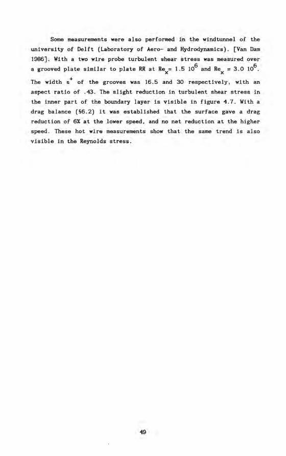
Some measurements were also performed i l the windtunnel of the

university of Delft (Laboratory of Aero- and Hydrodynamics). [Van Dam

1986]. With a two wire probe turbulent shear stress was measured over

a grooved plate similar to plate RR at Re = 1.~ 106 and .Re = 3.0 106 . x x

The width s+ of the grooves was 16.5 and 30 respectively, with an

aspect ratio of .43. The slight reduction in turbulent shear stress in

the inner part of the boundary layer is visibie in figute 4.7. With a

drag balance (§6.2) it was established that the surface gave a drag

reduction of 6% at the lower speed, and no net reduction at the higher

speed. These hot wire measurements show that I the same .trend is also

visible in the Reynolds stress.

49

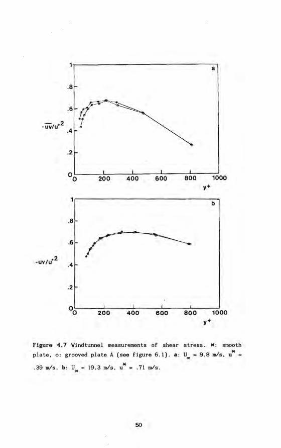
1 a

.8

~' .6

11 . -uv/u*2 1

.4

.2

00 200 400 800 1000 y+

1 b

.8

.6

*2 -uv/u .4

.2

00 200 400 600 800 1000 y+

Figure -4.7 Windtunnel measurements of shear stress. *: smooth

plate, 0: grooved plate A (see flgure 6.1) . U = 9.8 mis, * a: u = IlO

. 39 mis. b: U IlO

= * 19 .3 m/s, u = .71 mis .

50

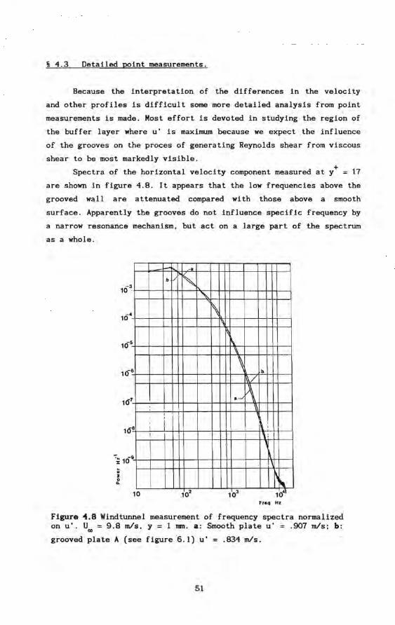
§ 4.3 Detailed point measurements.

Because the interpretation of the differences in the velocity

and other profiles is difficult some more detailed analysis from point

measurements is made. Most effort is devoted in studyin~ the reglon of

the buffer layer where u' is maximum because we expect the influence

of the grooves on the proces of generating Reynolds shear from viscous

shear to be most markedly visible.

Spectra of the horizontal velocity component measured at y+ = 17

are shown in figure 4.8. It appears that the low frequencies above the

grooved wall are attenuated compared with those above a smooth

surface. Apparently the grooves do not influence specific frequency by

a narrow resonance mechanism, but act on a large part of the spectrum

as a whoie.

:; J o ...

1Ö 5

6

7 1Ö

1Ö 8

9

10

- LOL

bV ~ ""-

, , i

! I

.10 2

r\ "I

\. '\ ,

b

~/

a--' P\ ~

,: \: ,

\

[1\ . 10

3 41 10

Freq Hz

Flgure 4.8 Windtunnel measurement of frequency spectra normalized on u'. U .. = 9.8 mis, y = 1 mmo a: Smooth plate u = .907 mis; b:

grooved plate A (see figure6.1) u' = .834 mis.

51

A different way of looking at the total velocity signal can be

obtained by calculating the velocity probabili ty function. As two

component measurements are available we can plot the joint probability

functions (Figure 4.9 to 4.11). From this joint probability density

p(u. v) the probability P that the velocity vector points in the

rectangle u ± Au/2. v ± Av/2 can be calculated with the formula:

u+Au/2 v+Av/2 N N

P J J p(u.v) du dv u-Au/2 v-Avl2

The lines shown in the figures are the iso-probability densi ty

contours of the probability distributions. As is weIl known. knowledge

of the shape of the distributions' enables one to calculate the

n th-order moments of the veloei ty distributions. In case of two

Gaussian distributed and correlated signals the contour lines would be

a set of nested ellipses with common center. The eccentricity of the

ellipses is a measure of the correlation between the two signais; in

our situation this correlation is related to the Reynolds shear

stress.

The measured contour lines are not ellipses and indicate thus a

deviation from normal gaussian signal which is to be expected. The

fact that the inner contour lines are less tilted than the outer can

indicate that the events which cause the velocityvector to point far

from its ave rage position (the center) contribute more to the Reynolds

shear as can be expected from their amplitude only . This effect is

most pronounced above the smooth plate.

The probability distributions presented in figure 4.10 are ft

obtained at 2.5 mm ( ~ 17 v/u) above the surface (reckoned from the

top of the roughness elements) at 140 mm1s free stream velocity. The

graphs show some subtle differences between measurements above the

longitudinal grooved plates SS and SA and the two other plates UU and

CG. Most apparent is the shift of the position of the maximum of the

distribution from the fourth quadrant to the centre. The difference is

visible throughout the buffer layer and also in the lower part of the

logarithmic region as figure 4.11 illustrates.

Although this indicates strongly a difference in turbulent

structure of the flow above longitudinal grooved wall the connection

with the drag reducing mecbanism is unclear. Figure 4.9 shows the

52

same type of measurements at a free stream speed of 95 mm/s. which is

about the speed at which drag reduction occurs and those measurements

do not show obvious differences betweenthe different plates.

A different way of analysis of the boundary layer is by

detecting events associated with structures. Most interesting are of

course those events which are connected with momentum transport.

Turbulent burst detection [Blackwelder & Kaplan 1970J is one of those

methods al though there has been much discussion on i ts relevance to

shear stress generatlon [Kunen 1985] .

In the method of Blackwelder & Kaplan burst detection is done as A

follows. One defines a VITA-average (variabie interval time average) U

of the horizontal velocity component U(t) as being :

A

U(t) 1 f

m

T 12 + t m

J U(~) dt

-T 12 + t m

A

And in a similar way one defines U2 • the VITA-mean of U2 (t). A burst

is said to have occurred if the ratio between the mean turbulent

energy and the local time averaged mean becomes too large:

The burst frequency thus determined is still a funetion of the

parameters Tm and k. The dependence on Tm is weak but the dependence

on the detection level k is exponential. Therefore the last dependence

is shown explicitely in the figures 4.12 and 4.13. According to

johansson ea [19B4] the dependence of the measured burst frequency on

the distance from the wall is relatively weak. Between y+ = 15 and y+

= 50 the deviation in ave rage burst frequency is less than 20% (figure

4.14) .

The measurements show no reduction in burst frequency at the

lower velocity for the wall SA. but a clear increase in burst

frequency above the plates SS and CC~ At higher velocity the sequence

between the different plates is changed. Because events in which the

vertical velocity component is large. be it positive or pegative. have

53

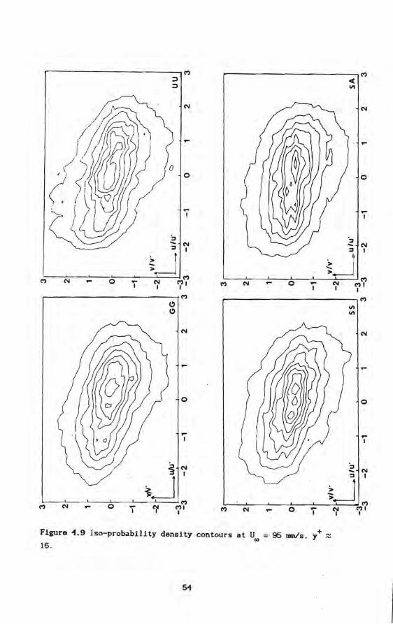
...-----------'----, M .------------,M

... ...

o o o

... ... I I

:, ":::I - N - N :::I I :::I I

~-1 ~~. M

0 N M M N ... 0 ... N 71 (') N ... ... MI I I I I I

M M C)

." C) ."

N N

...

o

... ... I I

i N ":::I N -I :::I I

~-1 ~-1 M M

M N ... 0 ... C)I MI M N ... 0 'j" C)I MI I I ..

Figure -1.9 Iso-probability density .contours at U = 95 IIIIlIs. y+ ::::: Q)

16.

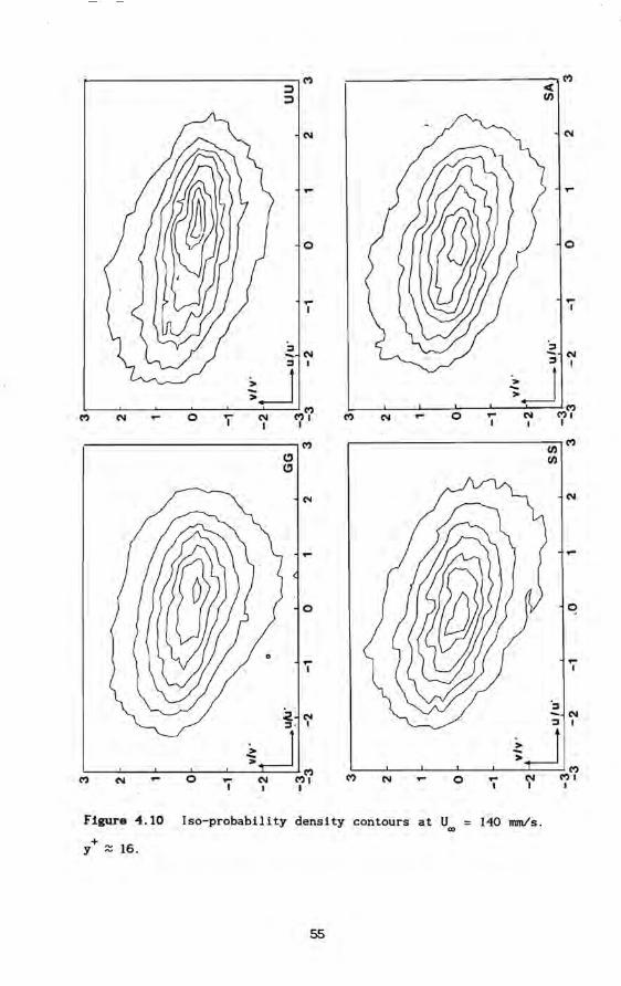
~-------------------------.M ________________________ ~M

cs: (/j

.-

o

.-I

~ (11 -:I I

~~ MM M (11 0 .- (11 M (11 .- 0

I I I I

M C) C)

C'I

.-

o

.-I

(11 .- o .-I

.- o

Figure 1.10 Iso-probability density contours at U~

y+ ~ 16.

55

.-

o

.-I

.:! (11 :I I

~~ .-I

.­I

(11

I

140 mm/s.

M MI I

(/j (/j

':1

M

(Ij

.-

.­I

(11 :I I

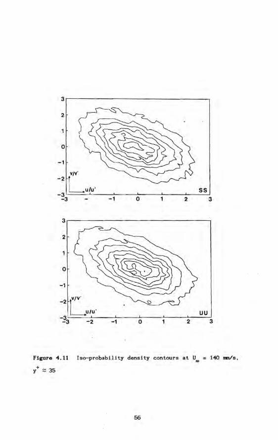
3

2

1

0

-1

-2 L u/u' SS

-3 -3 -1 0 1 2

3

2

1

0

-1

-2 LU/U--3

0 2 -3 -2 -1 1

Flgure ~.11 Iso-probability denslty contours at Um

y+ ~ 35

56

UU

3

3

HO JIIIIIs,

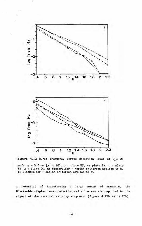
-1 N ~

0" Cl) ... --2 Cl)

o

a

-3+---~~--~--~~~~--~--~~ .4 .6 .8 1 1.2 k 1.4 1.6 1.8 2 2.2

o

N ~

0"-.5 Cl) ... -Cl) o

-1

.4.6 .8 1 1.2 1.4 1.6 1.8 2 2.2 k

Flgure 4.12 Burst frequency versus detection level at U = 95 '" + ~ mmls. y = 3.5 mm (y ~ 16). 0 : plate UU, +: plate SA, 0 : plate

SS, IJ. : plate .GG. a: Blackwelder - Kaplan criterion applied to u. b: Blackwelder - Kaplan criterion applied to v. .

a potentialof transferring a . large amount of momentum, the

Blackwelder-Kaplan burst detection criterion was also applied to the

signalof the vertical velocity component (Hgure 4.12b and 4.13b).

57

\

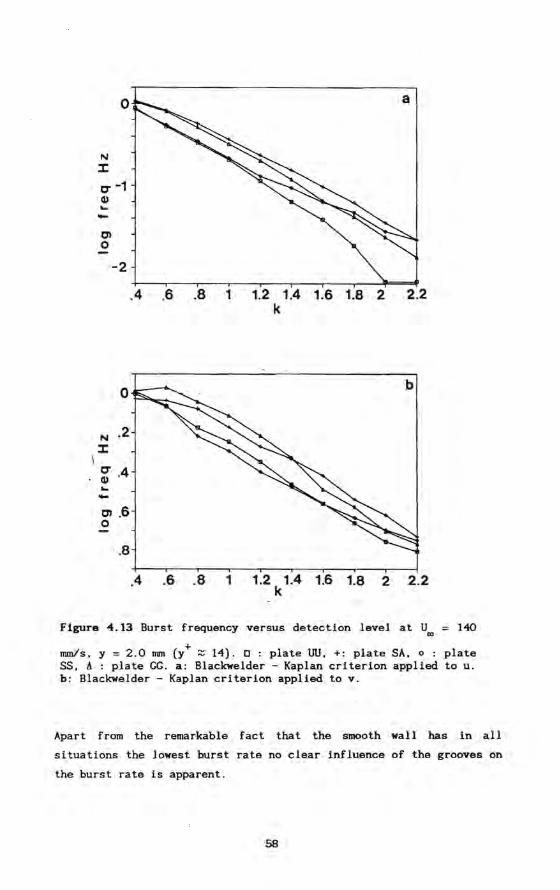
N l:

o

tr -1 Q) ... -en o

N l:

tr Q) ... -

-2

0

.2

.4

en .6 o

.8

.4 .6 .81

.4 .6 .8 1

1.2 1.4 1.6 1.8 2 k

1.2 1.4 1.6 1.8 2 2.2 k

Flgure 4.13 Burst frequency versus detection level at U = 140 '"

mmls. y = 2.0 mm (y+ ~ 14). D : plate UU. +: plate SA. 0 : plate SS. A : plate CG. a: Blackwelder - Kaplan criterion applied to u. b: Blackwelder - Kaplan criterion applied to v.

Apart from the remarkable fact that the smooth wall has in all

situations the lowest burst rate no clear influence of the grooves on

the burst rate is apparent.

SB

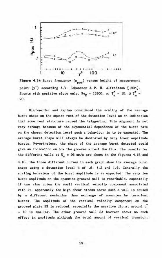
1/1 o 0-

e

1

.1

D_I!

1

0 __ 0 -°-0 0

o/' ~ 0- .=0.7 /' 0 _O-D-O_O

.-::::::..---- 0 -- c - 0

10 100

Flgure ~.1~ Burst frequency (npos) versus height of measurement

+ point (y ) according A. V. Johansson & P. H. Alfredsson [1984].

Events with positive slope only. ReD = 13800. 0: T+ = 10. 0 T+ m m

20.

Blackwelder and Kaplan considered the scaling of the ave rage

burst shape on the square root of the detection level as an indication

that some real structure caused the triggering. This argument is not

very strong; because of the exponential dependence of the burst rate

on the chosen detection level such a behaviour is to be expected. The

average burst shape will always be dominated by many lower amplitude

bursts. Nevertheless. the shape of the average burst detected could

give an indication on how the grooves affect the flow . The results for

the different walls at U~ = 96 mm/s are shown in the figures 4.15 and

4.16. The th ree different curves in each graph show the ave rage burst

shape using a detection level k of .8. 1.2 and 1.6. Generally the

scaling behaviour of the burst amplitude is as expected. The v·ery low

burst amplitude on the spanwise grooved wall is remarkable. especially

if one also notes the small vertical velocity component associated

with it. Apparently the high shear stress above such a wall is caused

by a different mechanism than exchange of momentum by turbulent

bursts. The amplitude of the vertical velocity component on the

grooved plate SS is reduced. especially the negative dip at around t+

= 10 is smaller. The other grooved wall SA however shows no such

effect in amplitude al though the total amount of vertical transport

59

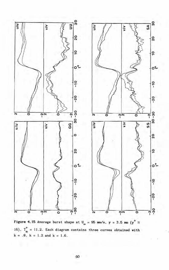
0 (ot) 0

c( M

(I)

0 N

0 N

0 ... 0 ...

0+- Ot...

0 0 ... ... I I

0 N

I

0 N ,

0 N M

J

0 NM I I

0 M ~ ~ '> ~ -..... .....

~ ~ ~ >

0 (I) M

(I)

0 0 N

0 0 N ...

O"t.. O~

0 0 ... ... I I

0 0 N N I I

0 N 0 NN 0 NM N

I I I

0 NM I I

Figure 4.15 Average burst shape at Um 95 mm/s. y = 3.5 IIID (y+ ~ +

16). Tm = 11.2. Each diagram contains th ree curves obtained with

k = .8. k = 1 . 2 and k = 1.6.

60

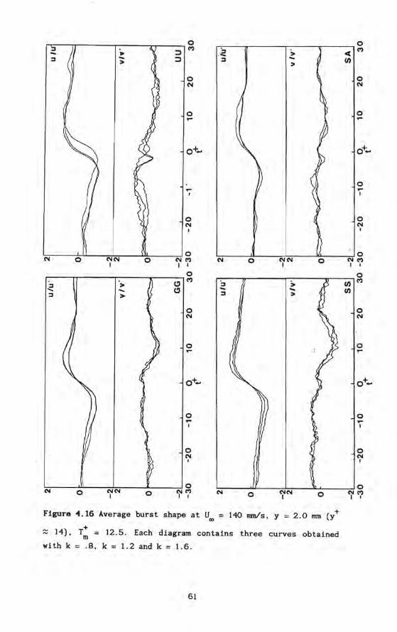
I> ... >

o N

o ...

.... I

o N

I

~N~----~U----:N~N~--~~----~N~g I I I

~--~~ ______ r-____ -r ____ ~O

" C")

" ::::J ..... ::::J

> >

o N

o

o ... I

o N

I

~--~r-------r-----,,--__ -,O ~ > ct C")

::::J -; IJ)

o N

o ...

o .... I

o N

I

L---------l.L..-----Nc'-N,..,....----""------='N g NOl I I

o ~~----w-------~->------~----IJ)-,. C")

'; "> IJ)

o N

o ...

o .... I

o N I

+ Flgure ~.16 Average burst shape at U~ = 140 mm/s, y = 2.0 mm (y

::: 14), T+ = 12.5. Each diagram contains three curves obtained m with k = .B, k = 1.2 and k = 1.6.

61

during the time the horizontal velocity component is less than

average. is smaller. This indicates a lower sh,ear stress transport

during an average burst.

§ 4.4 Conclusions .

The differences between the boundary layers over the different

plates. as can be measured wi th point measurements. are small. but

sometimes clearly significant. Much more difficult to establish is the

exact relation of these differences wi th momentum transport. Most

troublesome is the fact that many differences (in u'. and velocity

distribution and in the shape of the burst) become more pronounced at

higher veloeities outside the range of drag reduction.

The evidence points to the following general conclusion: above '

longi tudinal riblets the flow becomes more random (increasing burst

rate, more gaussian distribution of veloeities) and transports less

momentum (lower vertical transport per burst, less tilt of the outer

elliptic shaped iso-velocity contours). ,

The fact that the diffences become larger at higher veloeities

indicates that the original drag reducing mechanism still operates at

those veloeities but lts positive effect is eclipsed by the increased

devicedrag of the riblets penetrating into the logarithmic part of

the boundary layer.

A final piece of information from point measurements is derived

from the measured spectra. It appears that the spectra show no

resonance peaks and there seems to be no distinct frequency range

which is particularly affected by the presence of the grooves. This

indicates that if the drag reduction is caused by a kind of resonance

effect between the groove spacing and the turbulent structures (for

instance the relatively regular spaced low speed streaks), this

resonance must be very weak indeed.

62

Chapter 5 Hydrogen bubble visualisation.

§ 5.1 Introduction.

In recent years the study of turbulent boundary layer flow

phenomena has paid much attention to so-called "coherent structures".

Much effort has been devoted to conditional sampling with single point

measurements in order to detect and analyse the structures. But

visualisation studies show amore comprehensive view of the flow and

its regularities. They provided the stimulus in the application of the

eonditional single point measurements. Although visualisation gives a

good insight into the dynamics of the turbulent flow it has several

drawbacks. All visualisation techniques demand that markers are

introduced in the flow and the patterns they form tend to emphasize in

a stationary reference frame. the slow moving low speed streak. Short

high speed phenomena are not easily visualized. Moreover. it is

usually difficult and very timeconsuming to get quantitative results

from the visual pictures or films. Also the absolute aceuracy of the

measurements will be lower and noise in the measurements will be

higher in comparison wi th careful single point measurements. In an

attempt to partially remedy these disavantages we have used digital.

automated picture processing. This allows us to extract quickly

quantitative flow speed measurements from the pictures. As an

application of this method we eompare the flow of a turbulent boundary

layer over a smooth surface with the flow over grooved surfaces which

have drag reducing properties.

The total visualisation experiment eonsists of two types of

hydrogen bubble visualisation. Both experiments are done with a wire

at right angles with the free stream. parallel to the wall,

I Computer analysis of hydrogen bubble patterns. The video images

are obtained by photographing a single hydrogen bubble line a few

hunderd milliseconds af ter the voltage pulse. They are proeessed

wi th the computer and the output eontains the measured veloei ty

component in the mean flow direetion along a line. Simultaneously

LDA point measurements are made which are also recorded wi th the

hydrogen bubble information. A quantitative. statistical analysis

of the velocity profiles can be obtained. The method isespecially

63

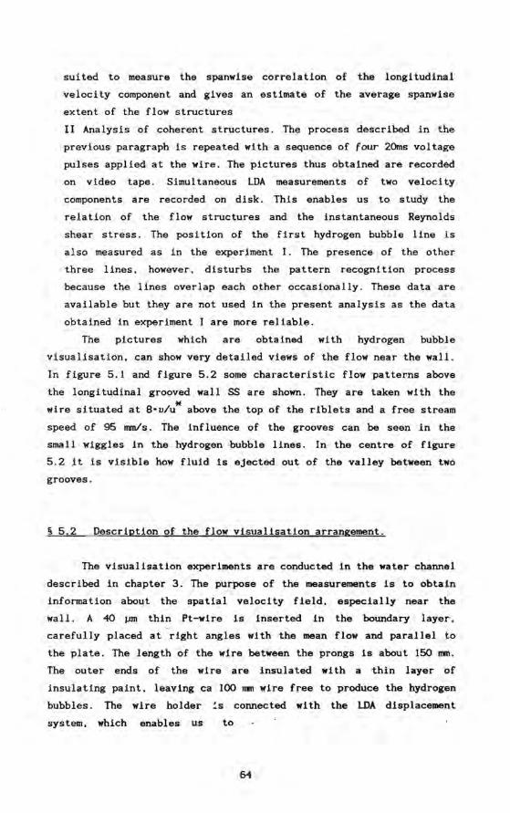
sui ted to measure the spanwise correlation of the long i tudinal

veloci ty component and gives an estimate of the ave rage spanwise

extent of the flow structures

II Analysis of coherent structures. The process described in the

previous paragraph is repeated with a sequence of four 20ms voltage

pulses applied at the wire. The plctures thus obtained are recorded

on video tape. Simultaneous LDA measurements of two velocity

components are recorded on disk . Thls enables us to study the

relation of the flow structures and the instantaneous Reynolds

shear stress. The position of the first hydrogen bubble line is

also measured as in the experiment I. The presence of the other

three lines. however. disturbs the pattern recognition process

because the lines overlap each other occasionally. These data are

available but they are not used in the present analysis as the data

obtained in experiment I are more reliable.

The pictures which are obtained with hydrogen bubble

visualisation, can show very detailed views of the flow near the wall.

In figure 5.1 and figure 5.2 some characteristic flow patterns above

the longitudinal grooved wall SS are shown. They are taken with the

wire situated at Sov/u* above the top of the riblets and a free stream

speed of 95 rrm/s. The influence of the grooves can he seen in the

small wiggles in the hydrogen bubble lines. In the centre of figure

5.2 it is vislble how fluid Is ejected out of the valley hetween two

grooves.

§ 5.2 Description of the flow visualisatlon arrangement.

The visualisation experiments are conducted in the water channel

described in chapter 3 . The purpose of the measurements is to obtain

information about the spatial velocity field. especially near the

wall. A 40 ~ thin Pt-wire is inserted in the boundary layer.

carefully placed at right angles with the mean flow and parallel to

the plate. The length of the wire hetween theprongs 15 about 150 mmo

The outer ends of the wire are insulated wi th a thin layer of

insulating paint, leaving ca 100 mm wire free to produce the hydrogen

bubbles. The wire holder !s connected with the LDA displacement

system, which enables us to

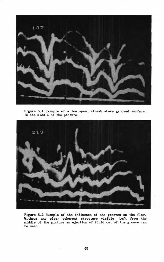
Flgure 5.1 Example of a low speed streak above grooved surface. In the middle of the picture.

Flgure 5.2 Example of theinfluence of the grooves on the flow. Without any clear coherent structure vlsible. Left from the middle of the picture an ejection of fluid out of the groove can he seen.

65

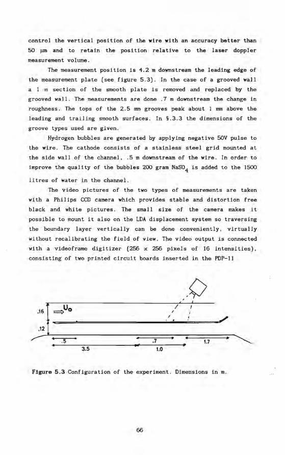
control the vertical position of the wire with an accuracy better than

50 ~ and to retain the position relative to the laser doppler

measurement volume.

The measurement position is 4.2 m downstream the leading edge of

the measurement plate (see figure 5.3). In the case of a grooved wall

alm section of the smooth plate is removed and replaced ' by the

grooved wall. The measurements are done .7 m downstream the change in

roughness. The tops of the 2.5 rnrn grooves peak about 1 rnrn above the

leading and trailing smooth surfaces. In §.3.3 the dimensions of the

groove types used are given.

Hydrogen bubbles are generated by applying negative 50V pulse to

the wire. The cathode consists of a stainless steel grid mounted at

the side wallof the channel •. 5 m downstream of the wire. In order to

improve the quality of the bubbles 200 gram NaS04 is added to the 1500

litres of water in the channel.

The video pictures of the two types of measurements are taken

with a Philips CCD camera which provides stable and distortion free

black and whi te pictures. The smal I size of the camera makes i t

possible to mount it also on the LDA displacement system so traversing

the boundary layer vertically can be done conveniently. virtually

without recalibrating the field of view. The video output is connected

with a videoframe digitizer (256 x 256 pixels of 16 intensities).

consisting of two printed circuit boards inserted in the PDP-11

/ .16 /

~====~================ __________ / ____ -c========-'~ .12

.5 • 7 • 1.7 3.5 1.0

Flgure 5.3 Configuration of the experiment. Dimensions in m.

66

minicomputer. In experiment 11 the reconstructed picture from the

digitizer data is recorded with a standard VHS video recorder .

LighUng is done wi th a 75W mercury lamp wi th a condenser and

lens system. so adjusted that parallel beam of light of 10 cm diameter

is directed to the hydrogen bubbles. In order to improve the contrast

between the lighted bubble pattern and the background the beam is

thrown through a slit of 5 mm width and 100 mm length. placed parallel

to the wall.

In order to clean the wire from largerbubbles and prevent the

accumulation of dirt particles which can destroy the uniformity of the

bubble production the wireholder can be electromechanically tapped.

This device operates very satisfactorily and makes prolonged

measurements without intervention possible. In the ,experiments the

Pt-wire was placed parallel to the wall. at right angles with the mean

flow. The laser beams of the LDA can be used to align the wire within

.3 mmo By applying a SOV pulse to the wire. a line of hydrogen bubbles

of ca 4~ diameter is generated.

In the experiments the pulsing of the wire. the tapping device.

the sampling of the LDA and the processing of the pictures is

controlled by the computer.

The measurements are obtained as follows. Af ter al1gning the

various components a thin plate of known dimensions is placed on the

plate in the water with its edge against (or very near) the wire. The

place of the four corners ABCD (figure 5.4) on the video frame is

registered. Af ter that the plate is removed and the waterspeed is

brought to its desired value. The computer now pulses the wire with a

vol tage pulse of 40 ms width. In experiment only one line is

generated; in experiment 11 Four lines are generated with a separation

of 140 ms at high speed and 260 ms at low speed. The command to

digitize is sent to the frame grabber af ter a delay of 140 ms and 260

ms at high and low free stream speed respectively. Within 20 ms the

digi tizing of a frame is started. Directly after digi tizing the, wire

holder is tapped to remove possible attached bubbles.

67

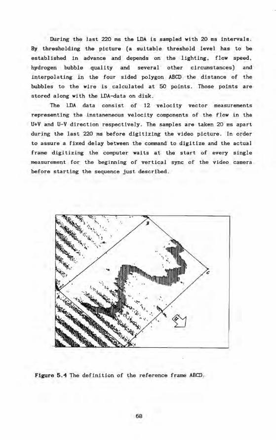
During the last 220 ms the LDA is sampled with 20 ms intervals.

By thresholding the picture Ca suitable threshold level has to be

established in advance and depends on the lighting. flow speed.

hydrogen bubble quality and several other circumstances) and

interpolating in the four sided polygon ABCD the distance of the

bubbles to the wire is calculated at 50 points. Those points are

stored along with the LDA-data on disk.

The LDA data consist of 12 velocity vector measurements

representing the instaneneous velocity components of the flow in the

U+V and U-V direction respectively . The samples are taken 20 ms apart

during the last 220 ms before digitizing the video picture . In order

to assure a fixed delay between the command to digitize and the actual

frame digi tizing the computer wai ts at the start of every single

measurement for the beginning of vertical sync of the video camera

before starting the sequence just described.

Flgure 5.4 The definition of the reference frame ABCD .

68

Now the sequence starts again and is repeated f ive hundred

times. The analysls of a picture takes about 1.5 seconds so the whole

measurement is done in 15 minutes. Afterwards the database of 500

veloei ty proflies and LDA measurements are avallable for further

analysis.

The experiments are performed at two different free stream 5 speeds, the lower being 96 mmls (Rex = 4·10 ) and the higher being 140

mmls (Rex 5.S.105 ). The surf aces studied are the smooth plate(plate

UU), the transverse grooved plate (plate CC) and two longitudinal

grooved plates, the plates SA and SS. Experiment 11 was not performed

on plate SA so no vide.o films of the flQw are available. Visual

observation of the generated bubble patterns indicated no obvious

difference compared with the flow observed over the other grooved

plate SS.

Measurements with the LDA and a drag balance (see §6.6) indlcate

a drag increase of the spanwise grooved wall CC of about 20%. The

longi tudinal grooved walls SA and SS show at U.., = 95 mmls a drag

reduction of 4 and 2% respectively,and at U.., = 140 mmls they show a

drag tncrease of about 2 and 11%.

The vertieal position at whieh the wire is plaeed varied, but

was always measured from the tops of the roughness elements. The LDA

measurement volume is placed as near to the wire as possible, without

having the bubbles interfere with the laser beams. lts position is

measured with a mieroscope and located .7 ± .1 mm below the wire and

* 1.0 ± .2 mm upstream. The typical va lues of viscous length (v/u) at

the measurement posi tion above the smooth plate are 210 J.IIIl at the

lower speed and 150 J.IIIl at the higher speed so the differenee in height

is 3.3 and 4.7 viseous units respectively. For near wall measurements

this is not negligible, nevertheless the eorrelation coeffieient

between the hydrogen bubble veloeity and the LDA measurement is always

between .85 and .95.

69

§ 5.3 Comparison with LDA and additional checks of the method.

Some doubt can be expressed about the accuracy of the method and

the possiblity of introducing systematic errors . Apart from the

int rins ic scientific value of simultaneous LDA and visual measurements

the availability of the LDA makes some checks on the performance of

the visualisation procedure possible. Several effects influence the

flow patterns and flow velocities as determined with the hydrogen

bubble technique (see Grass [1971J). We summarize these:

I Separation effect. The hydrogen is generated at specific sites

at the surface of the wire, forms a bubble because of the surface

tension and af ter some delay the bubble is separated from the wire

and is able to follow the flow. This separation effect is

complicated and is presumably not only dependent on local velocity

but also on local shear. A study of the recorded video output of

the frame digitizer indicated a delay of approximately 50 ms

between the leading edge of the voltage pulse and the first

appearance of the bubbles.

II Wake effect. The hydrogen bubble is detached from the wire and

moves initially in the flow field distorted by the wire and other

bubbles. This effect was studied by Grass . In our case the effect

i s reinforced because we do not measure the Instanteneous bubble

velocity but its trajectory lntegrated over a certain time,

starting from the wire . lts lmportancecan be checked by measuring

with different time delays.

III Buoyancy effect. Due to the lower density of the bubbles their

movement is lnfluenced by the buoyancy force. It can be shown that

in our case this force is small compared with the viscous forces.

IV Inertial effect. Due to the lower density of the bubble it

will not follow the flow exactly. It can be shown that in our case

this effect is negliglble.

V Integration effect (horizontal movement) . Because of the

integration time necessary to let the bubblè pattern develop,

certain flow patterns of short duration and short length will be

attenuated.

VI Vertical movement. The vertlcal velocity component makes the

calculated velocity also dependent on the local horizontal velocity

gradient. Certain flow patterns will he emphasized or attenuated by

70

this effect.

VII Spanwise movement. Because of the spanwise velocity component.

the calculated streamwise component is associated wi th the wrong

z-position at the wire.

Despite all these effects we still have a correlation

coefficient between .85 and .95 between the horizontal velocity

measured with the LDA and the horizontal velocity calculated from the

hydrogen bubble pictures. A part of the difference is also caused by

"the separation of several viscous units between the wire and the

measurement volume. We can now determine a regression curve to convert

the H2 bubble velocity to the real veloei ty as determined wi th the

LDA . It remains to be established whether the residual error is

correlated with one of the above mentioned error sources.

In figure 5.5 the measured velocity of the hydrogen bubbles in

the turbulent boundary is plotted against the LDA measurements. It is

very clear that the calculated bubble velocity is systematically lower

than the LDA measurements: but no clear systematic. nonlinear

deviation from the regression curve is apparent. Because the

regression curve almost intersects the origin i t indicates an error

source proportional to the local velocity. Part of the error can be

explained by the difference in height "between the wire and the LDA

measurement volume. This difference (25%) however is too large to

explain the total error. The first two sources of error are probably

responsible for the remaining difference.

The possibili ty that the errors in measured veloei ty of the

bubbles is correlated with the local turbulent intensity is

investigated with the help of figure 5.6. In this figure the residual

error (the difference between the velócity measured with the LDA and

the velocity of the hydrogen bubble corrected wi th the regression

curve) is plotted against the local turbulent intensity. This

turbulent intensity is calculated from the twelve LDA samples

according to the formula:

. J 12 -2 UI = = I (U.- U) i=1 1

71

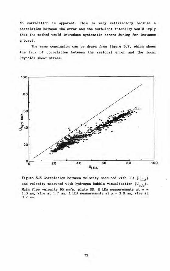
No correlation is apparent. This is very satisfactory because a

correlation between the error and the turbulent intenslty would imply

that the method would introduce systematic errors during for instanee

a burst.

The same conclusion can he drawn from figure 5.7, which shows

the lack of correlation between the residual error and the local

Reynolds shear stress.

100.-------------------------------------------~

.á ~ .a

80

60

-g, :f40

20

20 40 60 80

Flgure 5.5 Correlation between velocity measured with LDA (ULDA )

and velocity mèasured with hydrogen bubble visualisation (Ubub).

Main flow velocity 95 mm/s. plate SS. 0 LDA measurements at y = 1.0 mmo wire at 1 .7 mmo A LDA measurements at y = 3.0 mm, wire at 3.7 mmo

72

100

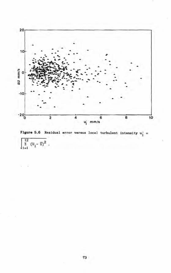
20~--------------------------------------------.

10

-10

....

a A

aa a A

·20L---------------+:-------~:__~---__::_----_:_! o 2 4 6 8 10 ui · mm/s

Flgure 5.6 Residual error versus local turbulent intensity ui

J 12 - 2 I (U i - U) . i=1

13

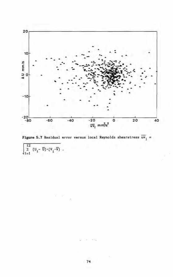
017 ï

H

1 1 1=1 r (~_oA)·(.!l -on) z~

lAn SSaJlSJ~aqs sPl0UÁaH l~ool SnSJ9A JOJJ9 l~nplsaH L"S 9~nall

~

•

OZ o

~

r.S~WW I~ OZ-

. .... .. ..... .. ... ...... ... ...

017-

... ......... ~..",... .., ... ....... ~;.;,. ........ .... ... .. ~- ...... ., ... ... ...... .. ..... -: :.It. .. ~..... ...

~ .-•• I·. ., -~~ • ....... ... ~" '-' .... ~ .... ... .. .,.--... ........ ..... .".

...... V ..... ·::~_· ..... ,,~...... .. .................... ... ........ ~... .... . ...

.. . --

09-

~

..

09-OZ-

O~-

t:-oe

3 3

I ...... lIJ

O~

~--------------------------------------------~----~IOZ

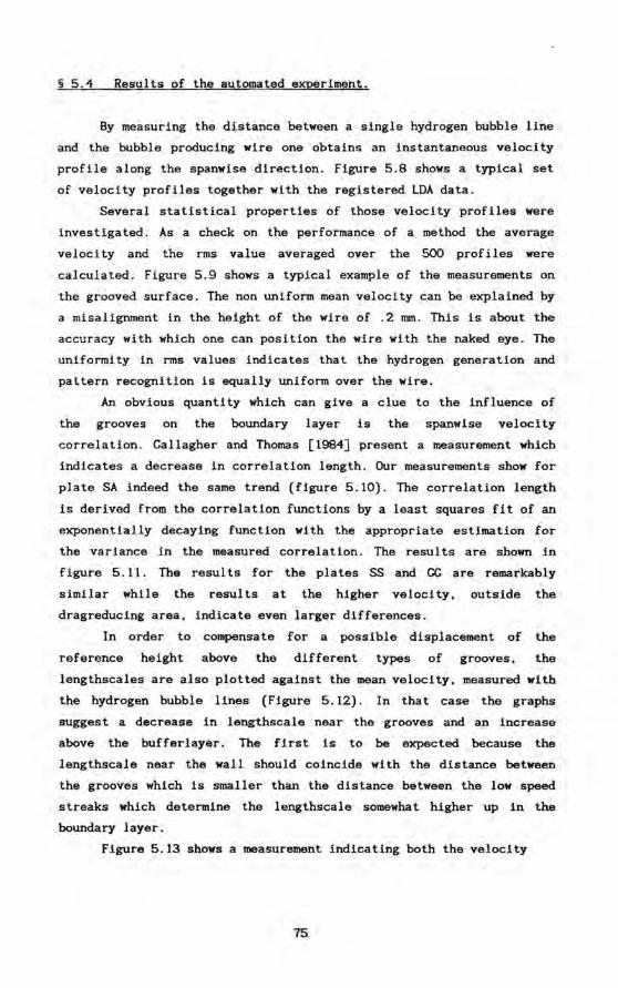
§5.4 Results of the automated experiment.

By measuring the distance between a single hydrogen bubble line

and the bubble producing wire one obtains an instantaneous velocity

profile along the spanwise direction. Figure 5.8 shows a typical set

of velocity profiles together with the registered LDA data.

Several statistical properties of those velocity .profiles were

investigated. As a check on the performance of a method the ave rage

velocity and the rms value averaged over the 500 profiles were

calculated. Figure 5.9 shows a typical example of the measurements on

the grooved surface. The non uniform mean velocity can be explained by

a misalignment in the height of the wire of .2 mmo This is about the

accuracy with which one can position the wire with the naked eye. The

uniformi ty in rms values indicates that the hydrogen generation and

pattern recognition is equally uniform over the wire.

An obvious quantity which can glve a clue to the influence . of

the grooves on the boundary layer is the spanwise velocity

correlation. Gallagher and Thomas [1984] present a measurement which

indicates a decrease in correlation length. Dur measurements show for

plate SA indeed the same trend (figure 5.10). The correlation length

is derivedfrom the correlatlon functions by a least squares fit of an

exponentially decaying funetion wi th the appropriate estimation for

the variance in the measured correlation. The resul ts are shown in

figure 5.11. The results for the plates SS and CG are remarkably

similar while the results at the higher velocity, outside the

dragreducing area, indicate even larger differences.

In order to compensate for a possible displacement of the

reference height above the different types of grooves, the

lengthscales are also plotted against the mean velocity, measured with

the hydrogen bubble lines (Figure 5.12). In that case the graphs

suggest a decrease in lengthscale near the grooves and an increase

above the bufferlayer. The first is to be expected because the

lengthscale near the wall should coincide with the distance between

the grooves which is smaller than the distance between the low speed

streaks which determlne the lengthscale somewhat higher up in the

boundary layer.

Figure 5.13 shows a measurement indicating both the velocity

75

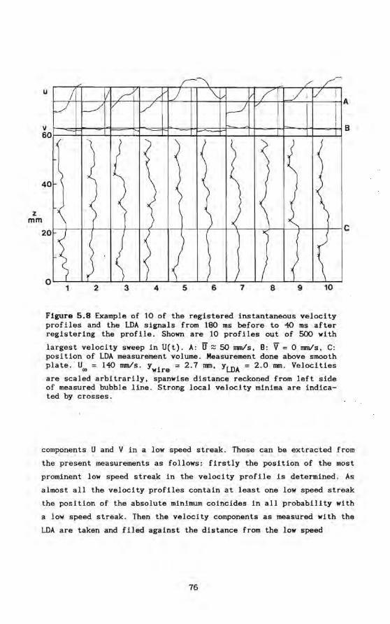
Flgure 5.8 Example of 10 of the registered instantaneous velocity profiles and the LDA signals from 180 ms before to 40 ms af ter registering the profile. Shown are 10 profiles out of 500 with

largest velocity sweep in U(t). A: IT~ 50 mmls, B: V = 0 mmls, C: position of LDA measurement volume. Measurement done above smooth plate. Uw = 140 mmls. YWire = 2.7 mm, YLDA = 2.0 mmo Veloeities

are scaled arbitrarily, spanwise distance reckoned from left side of measured bubble line. Strong local velocity minima are indica­ted by crosses.

components U and V in a low speed streak. These canbe extracted from

the present measurements as follows: firstly the position of the most

prominent low speed streak in the velocity profile is determined. As

almost all the velocity profiles contain at least one low speed streak

the position of thè absolute minimum coincides in all probabillty with

a low speed streak. Then the velocity components as measured with the

LDA are taken and filed against the distance from the low speed

76

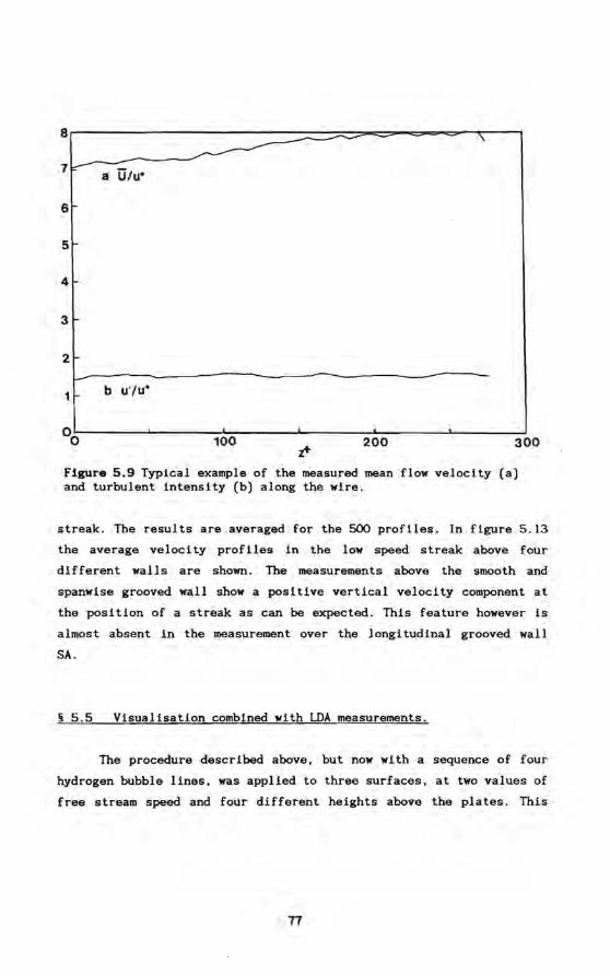
8 -7r::'" a U/u·

6

5

4

3

2

1 b U"/u·

00 100 200 300

Flgure 5.9 Typical example of the measured maan flow velocity (a) and turbulent intensity (b) along the wire.

streak. The results are averaged for the 500 profiles. In figure 5.13

the ave rage velocity proflles in the low speed streak above four

different walls are shown . The measurements above the smooth and

spanwise grooved wall show a positive vertical velocity component at

the position of a streak as can ba expected. This feature however is

almost absent in the maasurement over the longitudinal grooved wall

SA.

§ 5.5 Visualisation combined with LDA measurements.

The procedure described above, but now with a sequence of four

hydrogen bubble lines, was applied to three surfaces, at two va lues of

free stream speed and four different heights above the plates. This

17

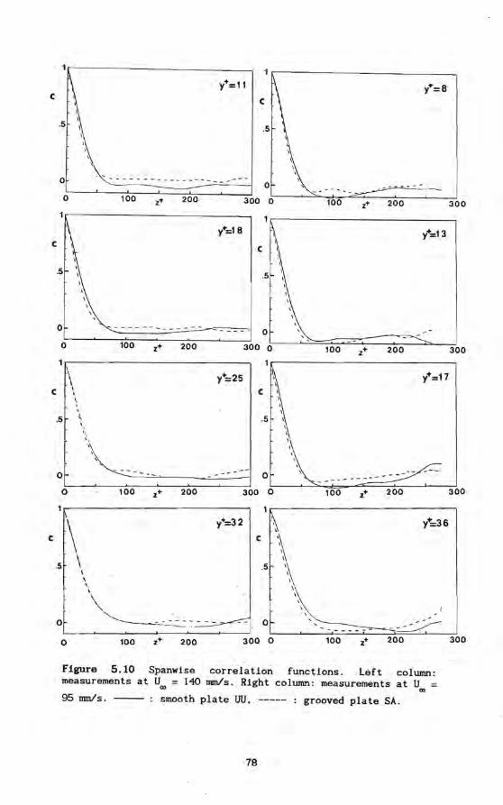
0 ... _----------------- -0

0 100 z+ 200 300 0 100 z+ 200 300

y+:18 t=13 c c

.5 .5

\

\

0 -------- - - - - :......:-- - - - - - 0

0 100 z+ 200 300 0 100 z+ 200 300 1

\ y+=25 y+=17

c \ C •

.5 ~ i

\ ..

0 \~-~---

0

0 100 z+ 200 300 0 100 z+ 200 300

1

\ /=32 y+=36

\

c c '\ .5 \ .5

\ , \ , \

\

\ \

\

0 ~-----,--.::::..: .~~ . 0 ---- ... -

0 100 z+ 200 300 0 100 z+ 200 300

Flgure 5.10 Spanwise correlation functions. Left column: measurements at U = 140 nun/s. Right column: measurements at U 00 (IJ

95 nun/s. --_ . smooth plate UU. ----- : grooved plate SA.

78

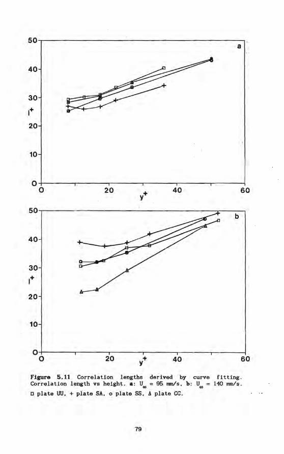
50.-----------------------------------------~ a

40

10

O+------,-------.------.------r------~----~ o 20 40 60

50~------------------------------~~--r_--~ b

40

20

10

O+------.-------.------.-----~------~----~ o 20 + y 40 60

Figure 5.11 Correlation lengths derived by curve fitting. Correlation length VB height . a: Um = 95 mrn/s, b: Um = 140 mrn/s .

o plate UU, + plate SA, 0 plate SS, A plate CG.

79

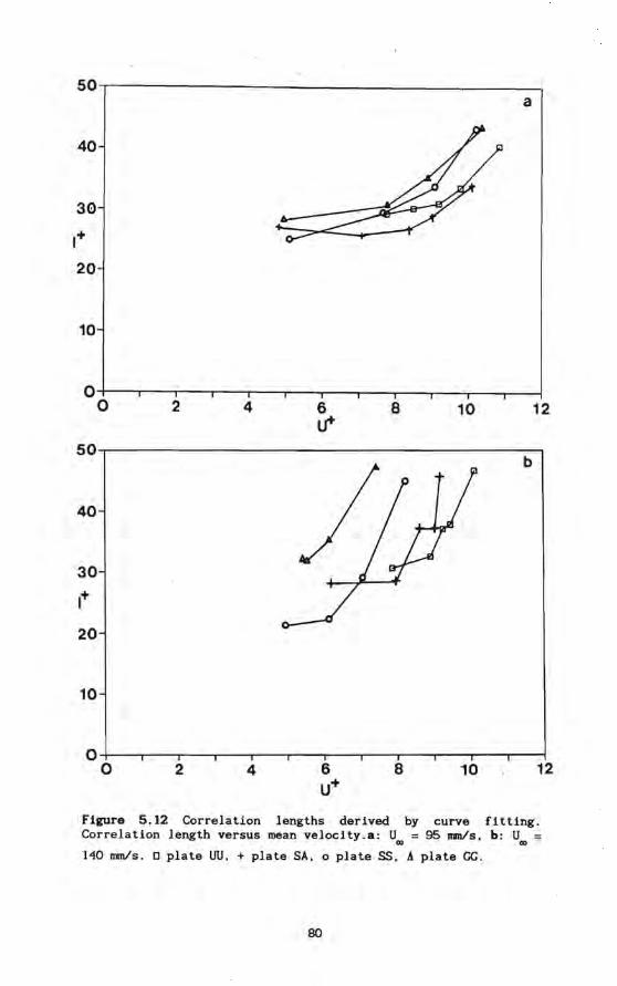
50,---------------------------______ ------. a

40

30

10

o~--.-~---.--~--~--~~--~--~--~~~~ o 2 4 8 10 12

50~--------------------------------------~ b

40

20

10

O+---~~--~--~~---.--._--.__.--_r--._~

o 2 4 8 10 12

F1gure 5.12 Correlation lengths derived by curve fitting. Correlation length versus mean velocity . a: Uw = 95 mm/s. b: Um =

140 mmls. D plate UU. + plate SA. 0 plate SS. A plate cc.

80

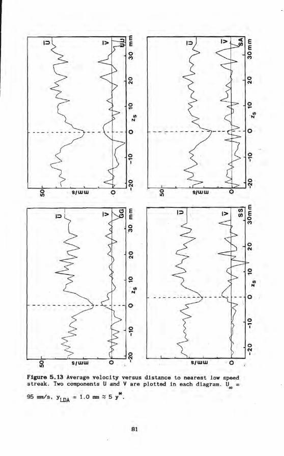
I::::)

o 11) S/WW

SI WW

Figure 5.13 Average velocity versus distance to nearest low speed streak. Two components U and Vare plotted in each diagram. Uoo

* 95 mm/s. YLDA = 1.0 UIII ~ 5 Y .

81

leads to 24 sets of 500 two second pieces of flow visualisation and so

about 7 hours of recordings are available for analysis.

A total analysis of the recordings was not made. Effort was

concentrated on the sequences taken at the lower velocity at 1 and 3

mm distance from the wall . The laser doppler data are used to select

the sequences. Wi th the data we can calculate the Reynolds stress

produced during the last 240 milliseconds of the recorded sequences.

The local Reynolds stress is calculated using the formula:

12

T = 1 (U - U) • (V - v) i i

i

U and Vare the velocity components averaged over all the 500

sequences.

The 500 sequences are thus ranked according to the value of the

Reynolds stress. Figure 5.14 shows the measured Reynolds stress of a

sequence plotted against its rank number in the sorted sequences. The

twenty sequences with the highest stress and the twenty sequences with

the lowest stress were studied in more detail. Both sets are indicated

in figure 5.14. Twenty random selected sequences we re also analysed.

It appears that indeed a large part (ca 30%) of the Reynolds stress.

be it positive or negative. is produced during the selected sequences.

So al though twenty (or in total 40) may seem limited. the selected

samples cover a large part of the stress production and are therefore

highly significant.

The peaked nature of the Reynolds stress distribution has been

known for a long time and .is sometimes considered an argument that

Reynolds stress is produced in highly localized regions. The key

question is whether those periods of high stress production are

associated with clearly recognizable flowpatterns.

The video sequences of the flow were categorized on the basis of

the observed patterns near the LDA measurement volume in order to make

our impressions morè objective. There are five ~in structures to be

distinguised:

I The longitudinal vortex.

82

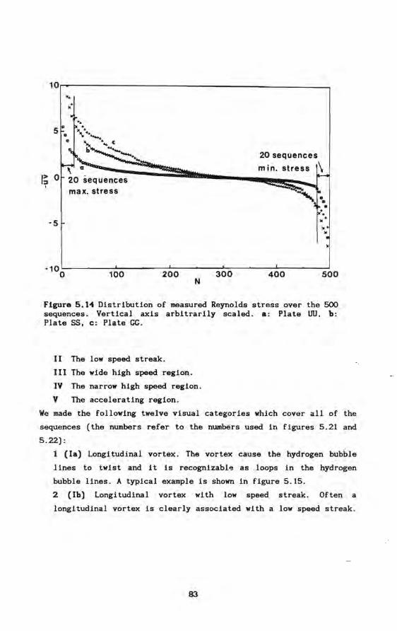
10 ,.. . •

. . . . . "" .. -. ... c ...... ....... 20 sequences

min. stress \ I~ 0 20 sequences

max. stress

-5

-10~--~--~----~--~----~--~--~----~--~--~ o 100 200 300 400 500

N

Flgure 5.1~ Distribution of measured Reynolds stress over the 500 sequences. Vertical axis arbitrarlly scaled. a: Plate UU. b: Plate SS. c: Plate CG.

II The low speed streak .

III The wide high speed region.

IV The narrow high speed reglon.

V The accelerating region.

We made the following twelve visual categories which cover all of the

sequences (the numbers refer tothe numbers used in figures 5.21 and

5 . 22):

1 (Ia) Longitudinal vortex. The vortex cause the hydrogen bubble

!ines to twist and it is recognlzabl'=! as .loops in the hydrogen

bubble lines. A typical example is shown in figure 5.15.

2 (Ib) Longitudinal vortex with low speed streak. Of ten a

longitudinal vortex is clearly associated with a low speed streak .

83

This is recogn1zed as a separate category although this comb1nation

could be a logical development of an intense low speed streak.

3 (1Ia) End of a low speed streak. If the four bubble lines showed

all a minimum at the same spanwise distance and the minimum was

clearly disappearing. this was catalogued as an end of a low speed

streak. A different ülterpretat!on could be that the top of the

streak temporarily went below tbe w1re height. Because no video

pictures directly after digitizing were avallable. an eventual

reappearance of the streak at the same placecould not be observed.

A typicalexample of this pattern is figure 5.16.

4 (IIb) Low speed streak. (figure 5.17). If all four hydrogen

bubble lines show a progressive V-shaped minimum this is taken as a

low speed streak. The difference hetween Ila and Ilb is clearer in

the moving video because one then also observes the folding of the

lines to a increasingly V-shaped minimum. This last aspect is

absent from category IIa.

5 (1Ic) Side of a low speed streak.

6 (lila) Side of a high speed region. The distinction between this

category and category IIc is a bit diffieult as low speed streaks

are of ten adjacent to high speed regions. The decision is made on

the basis of whether the local veloeity is higher than the average

between the maximum veloe1 ty in the high speed region and the

minimum velocity in the low speed streak. No distinction has been

made between the sides of the different high speed regions (111 and

IV) .

7 (IIlb) Narrow high speed region. This could also be ealled a high

speed streak although the maximum is not extremely peaked.

8 (IVa) Wide high speed region. This term is used for an area in

which the veloeity is higher than average and where the velocity is

more or less constant along the z-direction. No very distinguished

maximum can he located. Figure 5.18 shows a typièal example.

9 (IVb) End of high speed region. If a new minimum appeärs in a

wide high speed reg ion or a high speed area evolves into a less

pronounced feature this is ealled the end of the high speed region.

The ends of the different type of high speed regions are not

separated out beeause of the difficulty of recognizing the specifie

type at the end of its existence on video.

84

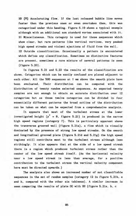
10 (V) Accelerating flow. Ir the last released bubble line moves

faster than the previous ones or even overtakes them. this was

categorized under this heading. Figure 5.19 shows a typical example

although with an additional non standard vortex associated with it.

11 Miscellaneous. This category is used for those sequences which

show clear. but rare patterns like verticalvortices . very peaked

high speed streaks and violent ejections of fluid from the wall.

12 Outside classification. Occaslonally a pattern is encountered

which defie's any classification. Sometimes no distinctive features

are present. sometimes a rare mixture of several patterns is seen

(figure 5.20).

In figures 5 . 21 and 5.22 the results of the classification are

shown. Categories which can be easily confused are placed adjacent to

each other. All the 500 sequences at 1 mm above the smooth plate have

been evaluated. Their distribution can be compared wi th the

distribution of twenty random selected sequences. As expected twenty

samples are not enough to oblain an accurate distribution over 12

categories but as those twelve categories can be divided infour

essentially different patterns the broad outline of the distribution

can be taken as what can he expected from a comprehensive analysis.

lt appears that most of the turbulent stress at the lower + investigated height (y = 8. figure 5 .21) is produced in the narrow

high speed regions (category 7). This is particulary apparent above

the transverse grooved wall (figure 5.21a). a flow which is visually

dominated by the presence of strong low speed streaks. On the smooth

and longitudinal grooved plate (figure 5.21d and 5.21g) the high speed

regions still contribute most to the turbulent stress al though less

strikingly . It also appears that at the side of a low speed streak

there is a region which produces turbulent stress rather than the

center of the low speed streak itself. (As the horizontal velocity

near a low speed streak is less than average. for a positive

contribution to the turbulent stress the vertlcal velocity component

here must be 'directed upwards.)

The analysis also shows an increased number of not classifiable

sequences in the set of random samples (category 12 in figure 5.21b. e

and h. compared with the other .six tableaus). A similar increase is

seen comparing the results of plate CG with UU (figure 5.21a. b. c

85

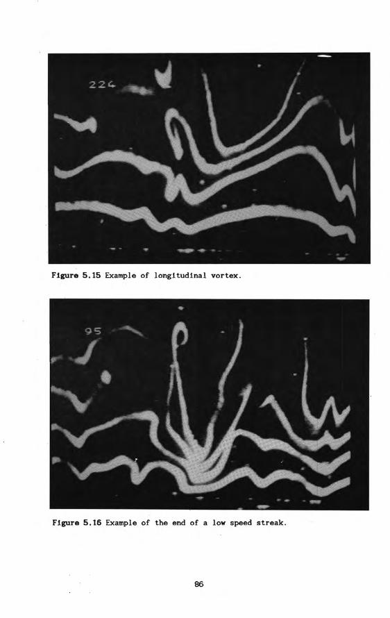
Flgure 5.15 Example of longltudinal vortex.

Flgure 5.16 Example of the end of a low speed streak .

86

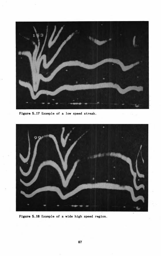
Flgure 5.17 Example of a low speed streak.

Flgure 5.18 Example of a wide high speed region.

87

~ .

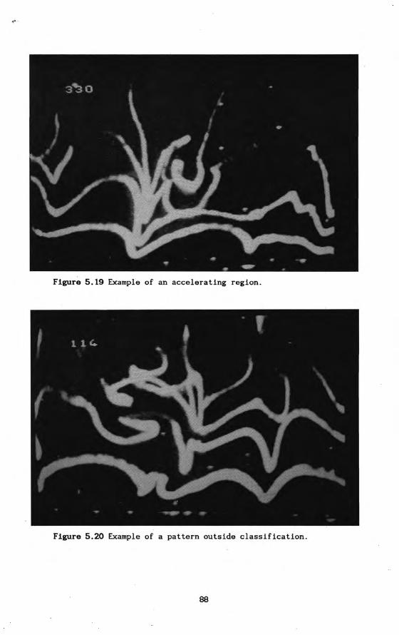
Flgure 5.19 Example of an accelerating region.

Flgure 5.20 Example of a pattern outside classification.

88

with 5.21d, e, f) or comparing UU with SS (figure 5.21d, e, f with

5.21g, h, i). This can be explained by the more chaotic behaviour of

the flow above the longitudinal grooves compared with the smooth and

spanwise grooved wall. + Higher up in the boundary layer (y = 17, figure 5.22) the

contribution of the high speed regions to the turbulent stress

distribution decreases compared to their contribution at y+= 8. If we

compare the number of their occurrences at a single height between the

different plates in the set of sequences of maximum stress we see a + relative decrease at y = 8 (comparing 5.21a with 5.21d and 5.2Ig) but

a relative increase at y+= 17 (comparing 5.22a with 5.22d and 5.22e).

This implies that the role of these structures in producing Reynolds

stress is different at different heights.

§ 5.6 Conclusions.

From the analysis of the combination of the visualisation

measurements with LDA measurements we can draw the folloWing

conclusion. Automatic visualisation and simultaneous LDA measurement

is quite possible. Correlation between bath methods is good;

Correlation coefficient is between .9 and .95 for the instantaneous

U-velocity component. No correlation between the velocity measured by

hydrogen bubble visuallsation and local shear stress, or turbulent

intensity is observed. This sustains the belief that the method gives

an accurate view of the relative veloeities (rather than . other

physical quantities as for instance shear stress) occuring in the

turbulent flow, despite the velocity defect induced by the wire.

The experimental resul ts show the following trends. Generally

the flow above longitudinal grooved surfaces is more chaotic than the

flow above a smooth wall. In the case of a spanwise grooved wall the

flow appears even more regular due to the presence of intense low

speed streaks. The measurement of spanwise correlatlon leads to

ambiguous results , caused by the difficulty of defining a suitable

reference height. Moreover both a more chaotic flow and a more intense

89

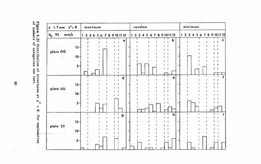
o ..., ...., ....

§~ y 1.7mm y+: 8 maximum random minimum

g"(11 Uo 95 mm/s 1 234 56 7 8 9101112 2 3 4 5 6 7 8 9 101112 23456 7 8 9 101112 ., . fII N a b c .... '1 I 0 I

""'0 I I ..... 15 C') fII I» t+ plate GG t+'1 (I) .... oqr::r o l:! 10 I I ., t+ ......... (I) 0 fII :::I 5 fII 0 (I) ...., (I)

fII t+ t+ d e I I (I)

~ >< I I t+ n

t+ 15 I l:! .,

plate UU I I (I) fII I I

I» 10 I

t+ I I

'<+ 5 11

ex>

'Tl 9 h 0 '1

(I) 15

~ plate SS ~

10 I» :::I ... ... I» t+ I I .... 0 5 :::I

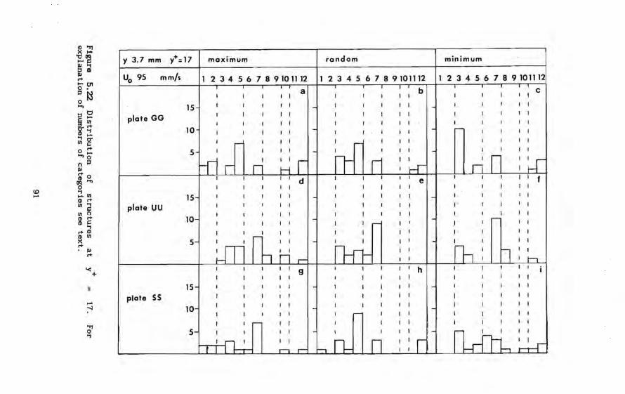
low speed streak patttern can apparrently lead to a decrease in

measured spanwise correlation length.

Although the visualisation plctures clearly show the presence of

the riblets. very little qualitative dlfference in structures

occurring on smooth plates and grooved plates could be detected .. only

some quantitative differences can be' observed. From comparison between

Reynolds stress measurements and flow visualisation. it appears that

no single structure can be identified which produces the bulk of the

Reynolds stress. The changes in wall shear stress of several per cent

are apparently not accompanied by major changes in flow

characteristics.

The conclusions of this chapter are in Hne wi th the main

conclusion of chapter 4 . Both single point measurements and

visualisation studies indicate that the flow above a longi tudinal

grooved wall is more chaotic than the flow above a smooth surface .

The visualisatlon does not show a clue why the turbulent

intens i ty above a longi tudinal grooved wall is 10% lower. compared

wi th a smooth wall. As no strikingly different structures are seen.

the dlfference must be due to some decrease in intens i ty of the

structures already present.

92

Chapter 6 Drag balance.

§6.1 Survey of different methods of measuring drag.

There exist several possibilities to measure the drag which is

exerted by a flow on the wall. Every method has its own advantages and

problems. Here we present a review of the available methods. We will

concentrate this discussion on the absolute accuracy of each method.

Prev ious measurements showed a maximum dràg reduction of about 5%

[Walsh 1979, Nitschke 1984]. So we will demand an accuracy of 2% or

better for our measurements.

§ 6.1.1 Indirect methods.

It is possible to measure the drag with indirect methods. We can

measure the Reynolds stresses or we can measure the velocity profile

and use lts shape to obtaln the wall shear stress.

The total shear stress in an equilibrium boundary layer can be

written as:

The theoretical relation

layer and the wal! shear

layer is [Townsend 1976]:

diT T ~ -p uv + v dy

between the shear stress

stress in the inner part

.T ~ + Y dP T

dx w

in the boundary

of the boundary

dP - -The ·measurement of dx' U(y) and uv(y) is needed to calculate the

drag. The first two quantlties are relatively easy to measure. The

Reynolds stress uv is much more difficult but it is the most important

quantity in the equation.

Except for the obvious difficul ty of measuring the U and V

components at the same position, two other problems beset the

measurement of uv. First one needs to calibrate the coordinate system

93

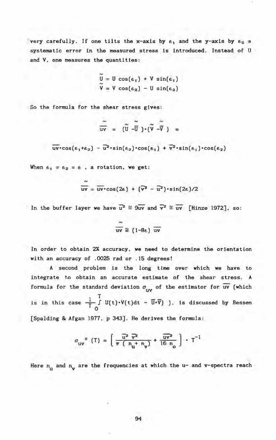
' very carefully. If one tiIts the x-axis by lö t and the y-axis by 1ö2 a

systematic error in the measured stress is introduced .. Instead of U

and V. one rneasures the quantities:

U U COS(löl) + V sin(löl)

V = V COS(1ö2) - U sin(1ö2)

So the formula for the shear stress gives:

uv (U -U )-(V -V

Iö a rotation . we get:

uv = uv-cos(21ö) + (y2 - U2)-sin(21ö)/2

In the buffer layer we have ~2 ~ 9uv and y2 ~ uv [Hinze 1972]. so:

uv ~ (1-81ö) uv

In order to obtain 2% accuracy. we need to determine the orientation

with an accuracy of .0025 rad or .15 degrees!

A second problem is the long time over which we have to

integrate t.o obtain an accurate estimate of the shear stress. A

formula for the standard deviation u of the estimator for uv (which uv 1 T

- f U(t)-V(t)dt- U-V) ) . T 0

is discussed by Bessem is in this case

[Spalding & Afgan 1977. p 343]. He derives the forrnula:

uuv 2 (T)

Here nu and nv are the frequencles at which the u- and v-spectra reach

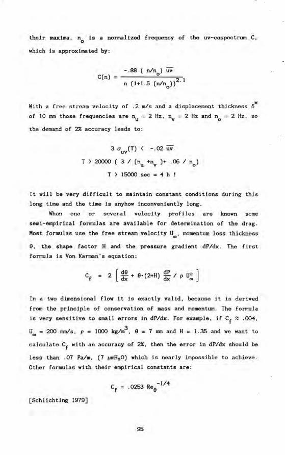
their maxima. n is a normalized frequency of the uv-cospectrum C, o

which is approximated by:

C(n) n (1+1.5 (nln ))2.1

o

With a free stream velocity of .2 mis and a displacement thickness ó*

of 10 mm those frequencies are nu 2 Hz , n = 2 Hz and n = 2 Hz, so v 0

the demand of 2% accuracy leads to:

3 0uv(T) < -.02 uv

T > 20000 ( 3 I (nu +nv )+ .06 I nol

T > 15000 sec = ~ h !

It will be very difficult to maintain constant conditions during this

long time and the time is anyhow inconveniently long.

When one or several veloei ty profiles are known some

semi-empirical formulas are available for determination of the drag.

Most formulas use the free stream velocity Ua>' momentum loss thickness

a, the shape factor Hand the pressure gradient dP/dx. The first

formula is Von Karman's equation:

Cf 2 [: + a· (2+H) : I p U! ]

In a two dimensional flow it is exactly valid, because it is derived

from the principle of conservation of mass and momentum. The formula

is very sensitive to small errors in dP/dx. For example, if Cf ~ .004,

U Q)

3 = 200 mm/s, p = 1000 kg/m , a 7 mm and H = 1.35 and we want to

calculate Cf with an accuracy of 2%, then the error in dP/dx should be

less than .07 Palm, (7 ~20) which is nearly impossible to achieve.

Other formulas with their empirical constants are:

[Schlichting 1979]

95

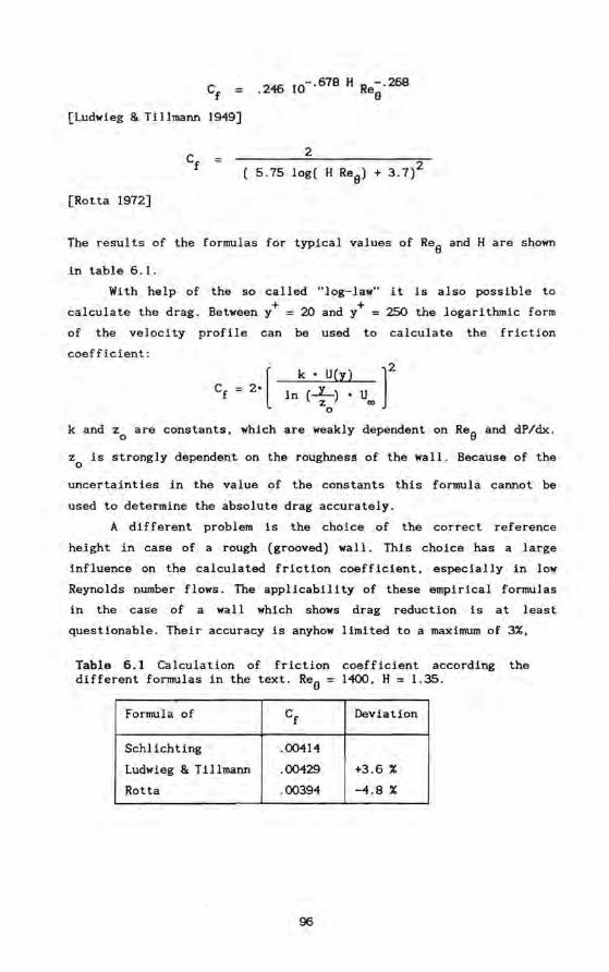
Cf .246 10-. 678 H Re~·268

[Ludwieg & Tillmann 1949]

[Rotta 1972]

2 2

5.75 loge H Rea) + 3.7)

The results of the formuias for typical values of Rea and Hare shown

in table 6.1.

With help of the so called "log-law" it is also possible to + + calculate the drag. Between y = 20 and y = 250 the logarithmic form

of the velocity profile can be used to calculate the friction

coefficient:

In (J.....) • U Z (11)

o

]2 k • U(y)

k and Zo are eonstants. which are weakly dependent on Rea and dP/dx.

Zo is strongly dependent on the roughness of the wall . Because of the

uncertainties in the value of the eonstants this formula cannot be

used to determine the absolute drag accurately.

A different problem is the choice of the correct reference

height in case of a rough (grooved) wall. This choiee has a large

influence on the calculated friction coefficient. especially in low

Reynolds number flows. Tbe applicability of these empirical formulas

in the case of a wall which shows drag reduction is at least

questionable. Their accuracy is anyhow limited to a maximum of 3%.

Tabla 6.1 Calculation of friction coeffieient aeeording the different formuias in the text. Rea = 1400. H = 1.35.

Formula of Cf Deviation

Schlichting .00414

Ludwieg & Tillmann .00429 +3.6 %

Rotta .00394 -4.8 %

96

because they contain constants derived from best fit procedures over a

wide range of experimental conditions. So it seems that drag

measurements based on point measurements or based on semi-empirical

formulas are not appropriate if we demand 2% accuracy.

A differerit indirect method is the use of hot film wall probes.

Here we use the theoretically founded idea that the amount of power

needed to maintain a piece of the wall at a certain temperature is

directly related to the local and instantaneous wall shear stress. But

even lf the problems of cal1brating such a device on a smooth wall

could be solved we would still face the problem of the different heat

transfer of a grooved wall. This would demand a separate calibration

for each of our grooved walls which makes this method useless in our

situation.

There are several other methods which depend on the existence of

a universa I velocity profile near the wall. for example Preston-tube

measurements. We wHI not discuss these methods as they are not

applicable to the flow above grooved walis.

§ 6.1.2 Direct methods.

A second group of methods can be called "Direct drag

measurements".We discern balance measurements and pressure drop

measurements. In the first method a part of the wall is disconnected

and suspended from a balance which measures the forces exerted on that

part of the wall. The forces are rather small in our si tuation:

because of the dlmenslons of our water channel the maximum area of

such a plate wHI be about .12 x .25 m2 and the drag force will be

about 2.5 mN. The resolution and accuracy we demand is 50 ~ (this is

equivalent to 5 mg). This force can be measured in several ways.

A second way of determining drag directly is the measurementof

pressure drop in a long straight pipe. The connection between the

pressure gradient and the wall shear stress in a pipe of diameter D

is:

The main conceptual difficulty is the definition of the pipe diameter

97

. wi th a rough wal 1. I f the roughness height is less than IX of the

diameter. the error associated with this problem is not significant so

we can calculate a minimum pipe-diameter for our measurements. Ihe

* optimal groove height is about 10 viscous units (y ) so:

* 10 y < .01 D

* An empirical formuia for y is [Schlichting 1979] :

* y -7/8

5 .03 D ReD

So ReD should be larger than 17000. A minimum height for accurately

machined grooves is .5 mm so the minimum D is 50 mmo Ihis implies a

pipe length of 10 m (100-D) which is needed to obtain a fully

developed turbulent flow. Ihe Reynolds number demands a flow velocity

of at least .34 mis in water (or 5 mis in air) which implies a minimum

volume of .7 lIs in water (or 10 lIs in air). The pressure gradient in

such a pipe will be:

dP dx=

2 16 -E2....- _ R 7/4

. 3 eD D

Over a length of 4 m we will measure a pressure difference:

AP 16 Pa in water (or 4.4 Pa in air)

For 2% accuracy we need a resolution of .32 Pa (32 J.UIlH20) in water

which is possible. We refralned from using a pipe circuit because data

were already available [Nitschke 1984]. Moreover. the difficulties of

performing visualisation studies in a pipe are much larger compared

with those of a flat plate. Also obtaining suitable pieces of piping

is more difficult than making grooved plates.

9B

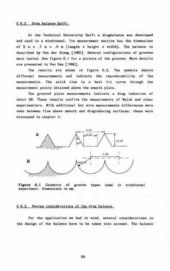
§ 6.2 Drag balance Delft.

At the Technical University Delft a dragbalance was developed

and used in a windtunnel. lts measurement section has the dimensions

of 5 m x .7 m x .9 m (length x height x width). The balance is

described by Van der Steeg [1985]. Several configurations of grooves

were tested. See figure 6.1 for a picture of the grooves. More details

are presented in Van Dam [1986].

The results are shown in figure 6.2. The symbols denote

different measurements and indicate the reproducability of the

measurements. The solid line is a best fit curve through the

measurement points obtained above the smooth plate.

The grooved plate measurements indicate a drag reduction of

about 6%. These results confirm the measurements of Walsh and other

experimenters. With additional hot wire measurements differences were

seen between flow above smooth and dragreducing surfaces; these were

discussed in chapter 4.

0 . 64

Flgure 6.1 Geometry of. groove types used in windtunnel experiment. Dimensions in mmo

§ 6.3 Design considerations of the drag balance.

For the application we had in mind. several considerations in

the design of the balance have to he taken into account. The balance

99

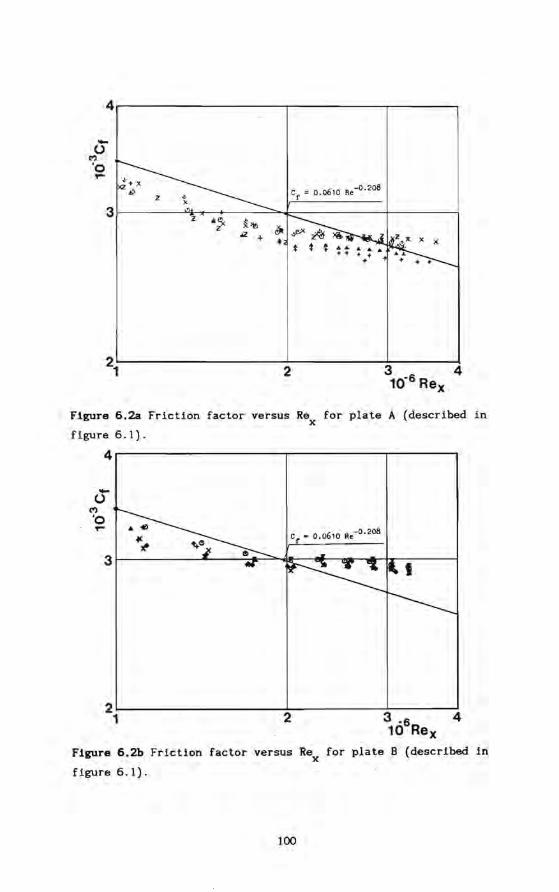
4r----------------,----------~----~

-u (')

'0 ,.. Cf = 0.0610 Re-0 . 208

3r-------~z~~----~~~--------~~------~ &~ ~'!>

.-z + ~ •

21~----------------2L---------~3------~4

10-6 Rex

Flgure 6.2a Friction factor versus Re for plate A (described in x

figure 6 . 1).

4r-----------------.----------.------~

-U (')

'0 ,.. C • 0.0610 Re -0.208

f

2~----------------~--------~------~ 1 2 3 -6 4

10 Rex

Flgure 6.2b Friction factor versus Rex for plate B (described in

figure 6.1).

100

has to opera te in water and if possible it must ba able to measure the

drag force in the range of speeds where the visualisation studies were

performed. Of course the balance has to fit in the channel wherethe

other experiments were performed. The following specifications.

therefore, must apply:

I Drag plate surface area ~ 120 x 250 nrn2 •

I I Sui table for measurements between .1 and .4 mis free stream

velocity.

111 Nominal dragforce (at .15 mis) 1.7 mN. IV Resolution and reproducibility ca 20 ~.

V Dragplate and its surroundings must be exchangeable.

VI The total apparatus should he as flat as possible. to minimize

its influence on the flow in the channel.

VII The apparatus must ba able to withstand water, if possible

slightly saline water.

Several possibil i ties exist for the construct ion of a sensor.

One can design a stiff balance with a sensor which measures the force

directly or one can measure the displacement of an elastically

suspended drag plate caused by the drag forces. But we must take into

account the dynamic range of 1:500 which we would like to have. The

detector must also operate without friction and without exerting force

on the plate.

Measuring with strain gauges falls in the first category, but

their sensitivity is just barely enough. Also there are problems of

slow aging and measuring small resistance changes under water. Also

considered were force transducers of piezoresisUve material which

would make for a very sUff suspension of the dragplate but their

mechanical stabili ty was insufficient. There is also the problem of

obtaining a low drift chárge amplifier, needed to re ad out the

devices.

To use the second method one must suspend the plate on small

springs and measure the displacement caused by drag. 8y choosing a

suitable stiffness. we can obtain the displacement desired.

Considering the relevant lengthscales a maximum displacement of .1 mm

seems acceptable, and the displacement sensor needs to have a

101

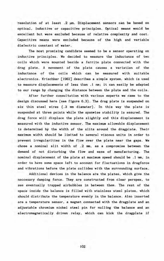
'resolution of at least .2 1JlII. Displacement sensors can he based on

optica!, inductïve or capaci tive principles . Optical means would be

excellent but were excluded hecause of relative complexity and cost.

Capacitive means were excluded because of the high and variabie

dielectric constant of water.

The most promising candidate seemed to be a sensor operating on

inductive principles. We decided to measure the inductance of two

coils which were mounted beside a ferri te plate connected wi th the

drag plate. A movement of the plate causes a variation of the

inductance of the coils which can be measured with suitable

electronics. Krischker [1982] describes a simple system, which is used

to measure displacements of less than .1 nm; it can easily he adapted

to our range by changing the distance hetween the plate and the coils.

Af ter further consul tation wi th various experts we came to the

design discussed here (see figure 6.3). The drag plate is suspended on

six thin steel wires (.3 mm diameter). In this way the plate is

suspended at th ree points while the spanwise stability is assured. The

drag force will displace the plate slightly and this displacement is

measured with the inductive sensor. The maximum allowabledisplacement

is determined by the width of the slits around the dragplate. Their

maximum width should he limited to several viscous units in order to

prevent irregularities in the flow over the plate near the gaps. We

chose a nominal slit width of .2 II'1II, as a compromise hetween the

demand of not , disturbing the flow and ease of manufacturing. The

nominal displacement of the plate at maximum speed should he .1 mm, in

order to have sorne space left to account for fluctuations in dragforce

and vibrations before the plate collides with the surrounding surface.

Additional devices in the balance are the plates, whlch give the

neccesary damping force. They are constructed from clear perspex, to

see eventually trapped airbubbles in between them. The rest of the

spac'e inside the balance is f!lled with stainless steel plates. which

should distribute the temperature evenly in the balance. Also inserted

are a temperature sensor, a magnet connected with the dragplate and an

adjustable chromium nickel steel pin for nulling the balance and an

electromagnetically driven relay, whlch can kick the dragplate if

102

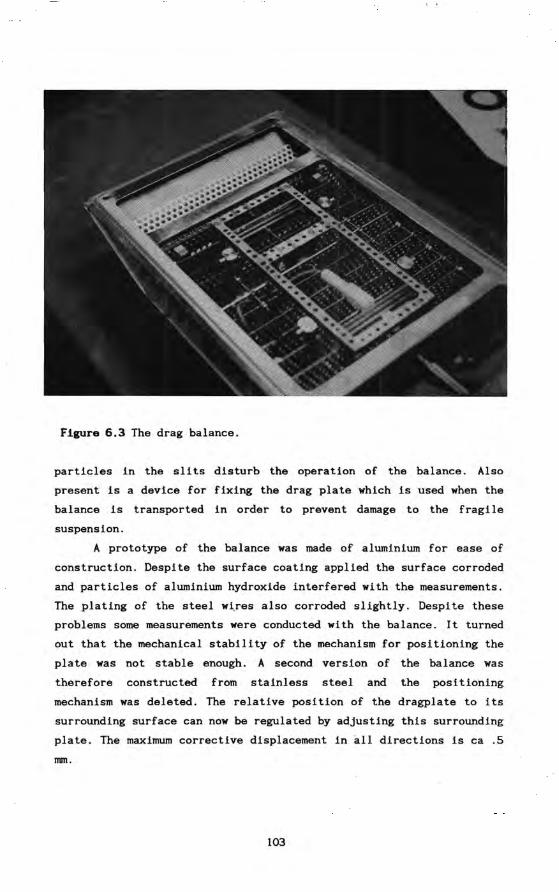
Flgure 6.3 The drag balance.

partic1es in the slits disturb the operation of the balance. Also

present is a device for fixing the drag plate whlch is used when the

balance is transported in order to prevent damage to the fragile

suspension .

A prototype of the balance was made of aluminium for ease of

construction. Despite the surface coating applied the surface corroded

and particles of aluminium hydroxide interfered with the measurements.

The plating of the steel wires also corroded slightly. Despite these

problems some measurements were conducted with the balance. It turned

out that the mechanical stability of the mechanism for positioning the

plate was not stabie enough. A second version of the balance was

therefore constructed from stainless steel and the positioning

mechanism was deleted. The relative position of the dragplate to its

surrounding surface can now be regulated by adjusting this surrounding

plate. The maximum corrective displacement in all directions is ca .5

mmo

103

In testing this second version several additional problems

surfaced. It appeared that leakage of the balance case could influence

the measurement drastically. Although this was known to be possible

from the very beginning, diagnosing it by excluding all other possible

defects and remedy it turned out to be very time consuming. Also some

small drift remained which was caused by water absorption in the

ferrite co re of the coils. Coating the coils in plastic and,

necessarily, mounting them differently solved the problem. The

influence of water absorption of the ferrite plate between the coils

can be minimized by keeping this plate constantly under water.

By now we can conclude that a lot of the problems which caused

the long development time of the balance originated from the use of

water as fluid in which the measurements were performed. Also

troublesome were the long timescales involved: it takes several

minutes to bring the channel to a new stable velocity and the

temperature time constant of the balance is about 15 minutes.

Refilling the channel causes a delay of at least one day because air

bubbles originate from the water preferentially in the sli ts of the

balance (at least there they are most apparent because of the problems

they cause).

§ 6.4 Some additional design formula of the balance.

The response of the position set) of the dragplate of the

balance to a force, can be thought as that of an ideal second order

system: 2

K ds - A s F(t) = M d s _

dt2 dt

Here F is the driving force, consisting of about five different

components.

I A fluctuating dragforce of ave rage value Tw-L-W (L-W is the

11

surface area), which we want to measure as accurately as

possible. dP

Unwanted pressure forces { dx L WH),

104

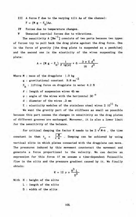
III A force F due to the vary1ng t1lt A~ of the channel:

F = (M g - Fh)Af.

IV Forces due to temperature changes.

V Unwanted inert1al forces due to vibrations.

The sensitiv1ty A [Nm-1] cons1sts of two parts because two types

of forces try to pull back the drag plate aga1nst the drag force. One

is the force of gravity (the drag plate is suspended as a pendulum)

and the second one is the elastici ty of the wires suspending the

plate:

Where M

g

mass of the dragplate

gravitat10nal constant

1.0 kg -2

9.S ms

Fh : lifting force on dragplate in water 4.2 N

e .p

d

E

length of suspension wires 45 mm

angle of the wires with the horizontal 30 0

diameter of the wires .3 mm

elasticity modules of the stainless steel wires 2 1011 Pa

We want the gravity part of the stiffness as small as possible

because this part causes the changes in sensitivity as the drag plates

of different grooves are exchanged . Moreover. it is also a lower limit

for the sensitivity of the balance.

For critical damping the factor K needs to be 2 ~ • the time

constant is then t = c J ~ . Damping can be achieved by using

vertical slits in which plates connected with the dragplate can move.

The pressures induced by this movement counteract the movement and

genera te a force proportional to the veloei ty. We can derive an

expression for this force if we assume a time-dependent Poiseuille

flow in the slits and the pressure gradient caused by it. We finally

obtain:

~L K = 12 p v --3-

D

With H

L

height of the slits

length of the 51its

D width of the slits

105

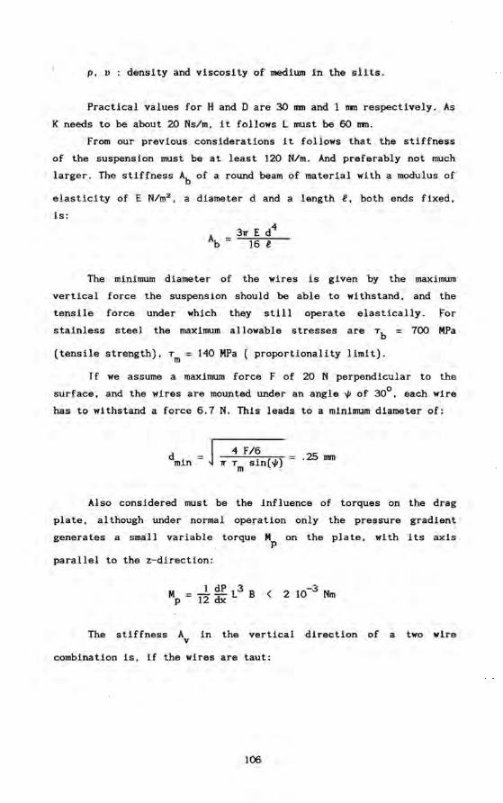
p, v density and viscosity of medium in the slits.

Practical values for H andD are 30 mm and 1 mm respectively. As

K needs to he about 20 Ns/m, it follows L must he 60 mmo

From our previous considerations it follows that the stiffness

of the suspension must be at least 120 N/m. And preferably not much

larger. Ihe stiffness Ab of a round beam of material with a modulus of

elasticity of E N/m2 , a diameter d and a length e, both ends fixed,

is :

3'1r E II 16 e

The minimum diameter of the wires is given by the maximum

vertical force the suspension should be able to wi thstand , and the

tensile force under which they still opera te elastically. For

stainless steel the maximum allowable stresses are Tb = 700 MPa

(tensile strength), T = 140 MPa ( proportionality limit). m

I f we assume a maximum force F of 20 N perpendicular to the

surface, and the wires are mounted under an angle ~ of 300 , each wire

bas to withstand a force 6.7 N. Ihis leads to a minimum diameter of:

J -4 F/6 'Ir T sin(~) m

.25 nin

Also considered must be the influence of torques on the drag

plate, al though under normal operation only the pressure gradient

generates a small variabie torque M on the plate, with its axis p

parallel to the z-direction:

M -L dP L3 B < 2 10-3 Nm p 12 dx

Ihe stiffness A in the vertical direction of a two wire v

combination is, if the wires are taut:

106

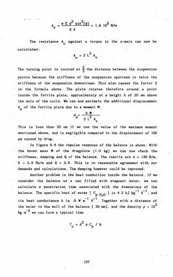
A v TE d2 sin2(+) = 1.6 105 N/m

2 I!

Tbe resistance Aw against a torque in the z-axis can now b~

calculated:

A 2 L2 A w v

2 The turning point is located at 3 the distance between the suspension

points because the stiffness of the suspension upstream is twice the

stiffness of the suspension downstream. This also causes the factor 2

in the formula above. Tbe plate rotates therefore around a point

inside tbe ferrite plate. approximately at a beigbt h of 20 mm above

tbe axis of tbe coils. We can now estimate tbe additional displacement

da of tbe ferrite plate due to a moment M:

d = ----=h.:.....::;M __ a 2 L2 A

v

This is less than 20 nm if we use tbe value of tbe maximum moment

mentioned above. and is negligible compared to tbe displacement of 100

~ caused by drag.

In figure 6.4 tbe impulse response of tbe balance is shown. Witb

the known mass M of the dragplate (1.0 kg) we can now check the

stiffness. damping and Q of tbe balance. Tbe results are A = 130 N/m.

K = 2.9 Ns/m and Q = 3.9 .. Tbis is in reasonable agreement witb our

demands and calculations. The damping however could he improved.

Another problem is the heat conduction inside the balance. If we

consider the balance as a can filled with stagnant water. we can

calculate a penetration time associated with the dimensions of tbe -1 -}

balance. Tbe specific heat of water ( Cp H2 0 ) is 4.2 kj kg K . and

its heat conductance k is .6 W m-1 K-1. Together with a distance of

the water to the wallof the balance ( 30 mm). and the density p = 103

kg m -3 can form a typical time we

T d2 p C / k c p

107

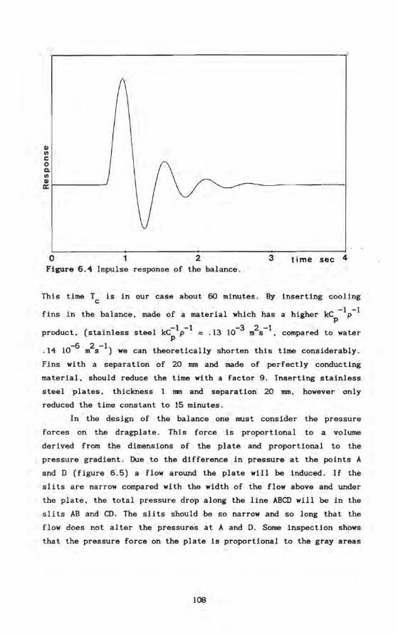
dl lil c: o Q. lil

~I-----~

o 1 2 Figure 6.4 Impulse response of the balance.

3 time sec 4

This time Tc is in our case about 60 minutes. By inserting cooling

-1 -1 fins in the balance, made of a material which has a higher kC p

p -1 -1 -3 2-1

product, (stainless steel kC p = .13 10 m s compared to water p

-6 2-1 .14 10 m s ) we can theoretically shorten this time considerably.

Fins wi th a separation of 20 mm and made of perfectly conducting

material, should reduce the time with a factor 9. Inserting stainless

steel plates, thickness 1 mm and separatiori 20 mm, however only

reduced the time constant to 15 minutes.

In the design of the balance one must consider the pressure

forces on the dragplate. Ihis force, is proportional to a volume

derived from the dimensions of the plate and proportional to the

pressure gradient. Due to the difference in pressure at the points A

and 0 (figure 6.5) a flow around the plate will he induced. If the

slits are narrow compared with the width of the flow above and under

the plate, the total pressure drop along the line ABCD will be in the

slits AB and CO. Ihe slits should be so narrow and so long that the

flow does not al ter the pressure"s at A and O. Some inspection shows

that the pressure force on the plate is proportional to the grayareas

108

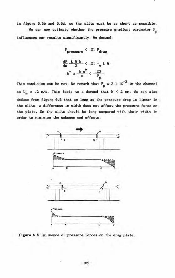
in figure 6.5b and 6.5d. 50 the slits MUst he as short as possible.

We can now estimate whether the pressure gradient parameter P p

influences our results significantly. We demand:

Fpressure < .01 Fdrag

dP L W h dx 2 < .01 T L W

w

* h+ = ~ < .02 v --P-p

Ihis condition can be met. We remark that P ~ 2.1 10-3 in the channel p

as U = .2 mis. Ihis leads to a demand that h < 2 mmo Wecan also Ol

deduce from figure 6.5 that as long as the pressure drop is linear in

the slits. a difference in width does not affect the pressure force on

the plate. So the slits should be long compared with their width in

order to minimize the unknown end effects .

A .. D :Cl J

1

z ~ ~

1 ,- - B

,

F ,~ A B C D

I Î~ EP'OUU_'O ---

- , ABC 0

Figure 6.5 Influence of pressure forces on the drag plate.

109

,§ 6.5 Sensor.

The sensor consists of two coils (diameter 22 mm) which are

separated by about 5 mmo In between is a ferrite plate, 4 mm thick,

extending at all sides at least 5 mm beyond the coils. This plate is

connected rigidly with the dragplate. The sensor is only sensitive to

the longitudinal component of the displacement of the dragplate. A

vertical or spanwise displacement due to the not absolute stiffness of

the suspension in those directions, will only have a marginal

influence on the sensor.

The electronic part of the sensor consists of a resonance bridge

in which the coils are included. The bridge is operated at its

resonance frequency of 45 kHz and the difference signal from the

brigde is measured with a lockin amplifier. The shielded leads from

the coils to the electronics were kept as short as possible (.5 m) to

avoid influence from parasitic capacities.

A main problem is the absorption of water in the coils, the

ferrite plate and the cabie, which causes a change of the electrical

resistance and stray capaci ty of the electronics . The problem was

solved by encapsulating the coils in araldite filled w!th quartz

powder and using tedious care in making and insulating the electrical

connections. By keeping the ferrite platelet always wet, its change of

magnetic permeability is brought to an acceptable low level. A plate

should be keptat least a week under water before it is stabie enough

to be used.

§ 6.6 Measurements and results.

Drag measurements were performed on six different surfaces with

at least two measurements on each surface. A measurement consisted

typically on measuring the ave rage drag as indicated by the balance

and the average free stream speed as indicated with the LDA during a

two minute period at a certain channel speed. A complete measurement

sequence consisted of about 25 measurement points, half of them during

the increase of free stream speed, the other half during the return to

zero speed. This enabled us to estimate the effects of drift due to

110

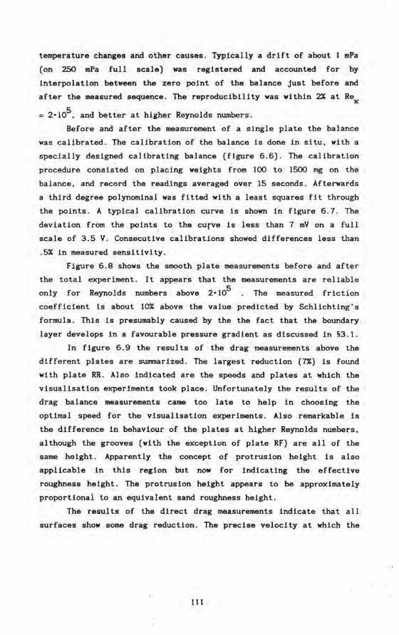
temperature changes and other causes. Typically a drift of about 1 mPa

(on 250 mPa full scale) was registered and accounted for by

interpolation between the zero point of the balance just before and

af ter the measured sequence. The reproducibility was within 2% at Rex

2.105 , and better at higher Reynolds numhers.

Before and af ter the measurement of a single plate the balance

was calibrated. The calibration of the balance is done in situ, with a

specially designed calibrating balance (figure 6.6). The calibration

procedure consisted on placing weights from 100 to 1500 mg on the

balance, and record the readings averaged over 15 seconds. Afterwards

a third degree polynominal was fitted with a least squares fit through

the points. A typical calibration curve is shown in figure 6.7. The

deviation from the points to the curve is less than 7 mV on a full

scale of 3.5 V. Consecutive calibrations showed differences less than

.5% in measured sensitivity.

Figure 6.8 shows the smooth plate measurements before and af ter

the total experiment. It appears that the measurements are rel1able

only for Reynolds numbers above 2.105 The measured friction

coefficient is about 10% above the value predicted by Schlichting's

formuia. This is presumably caused by the the fact that the boundary

layer develops in a favourable pressure gradient as discussed in §3.1.

In figure 6.9 the results of the drag measurements above the

different plates are summarized. The largest reduction (7%) is found

with plate RR. Also indicated are the speeds and plates at which the

visualisation experiments took place. Unfortunately the results of the

drag balance measurements came too late to help in choosing the

optima I speed for the visual1sation experiments. Also remarkable is

the difference in behaviour of the plates at higher Reynolds numbers,

although the grooves (with the exception of plate RF) are all of the

same height. Apparently the concept of protrusion height is also

applicable in this region but now for indicatlng the effectlve

roughness height. The protrusion height appears to he approximately

proportional to an equivalent sand roughness height.

The results of the direct drag measurements indicate that all

surfaces show some drag reduction. The precise velocity at which the

111

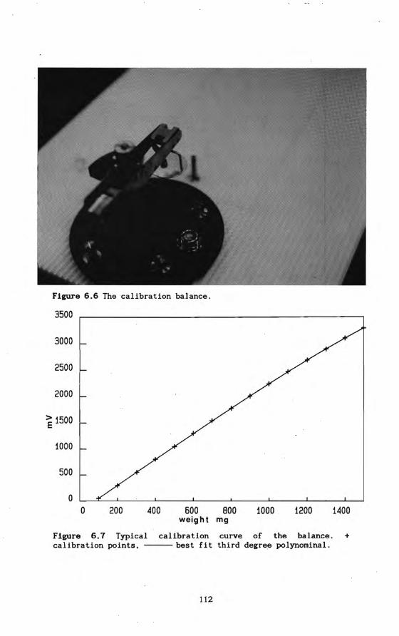
Flgure 6.6 The calibration balance.

3500

3000

2500

2000

~ 1500

1000

500

o o 200 400 600 800 1000 1200 1400

weight mg

Flgure 6.7 Typical calibration curve of the balance. + calibration points. -------best fit third degree polynominal.

112

+

7

+ ~

6 +

103C, + +

+ 1 5 + + t + + * +

-#" *. t 1: t * tt

t+) •• 4 1.2 1.5 2 3 4 5 6 8 10 l;-+t

·5 10 Rex

Flgure 6.8 Smooth plate drag measurements before and af ter all the grooved plate measurements.

maximum drag reductlon occurs is at a groove spacing s+ of Less than

15. somewhat contrary to the optimal spacing found by other authors.

There are several alternative explanations. Further research is needed

to decide which one applies:

I The sensitivity of the balance to pressure forces is

underestimated. rhe s11 ts along the grooved plates are somewhat

higher than those along the smooth plate so the grooved plates are

more and differently affected by the pressure forces.

11 Reynolds number effects. rhe measurements of the balance are

done at low Reynolds numbers near the transition to turbulence.

Ihis could affect the position of the optimum.

111 The drag reduced boundary layer is not completely adjusted to

the grooves. The beg inning of the drag plate is about 12 a downstream the change from smooth to grooved. the end is 37 a downstream the change. (These numbers are only approximate. the

exact values depend of course on the mean flow velocity) . It is

113

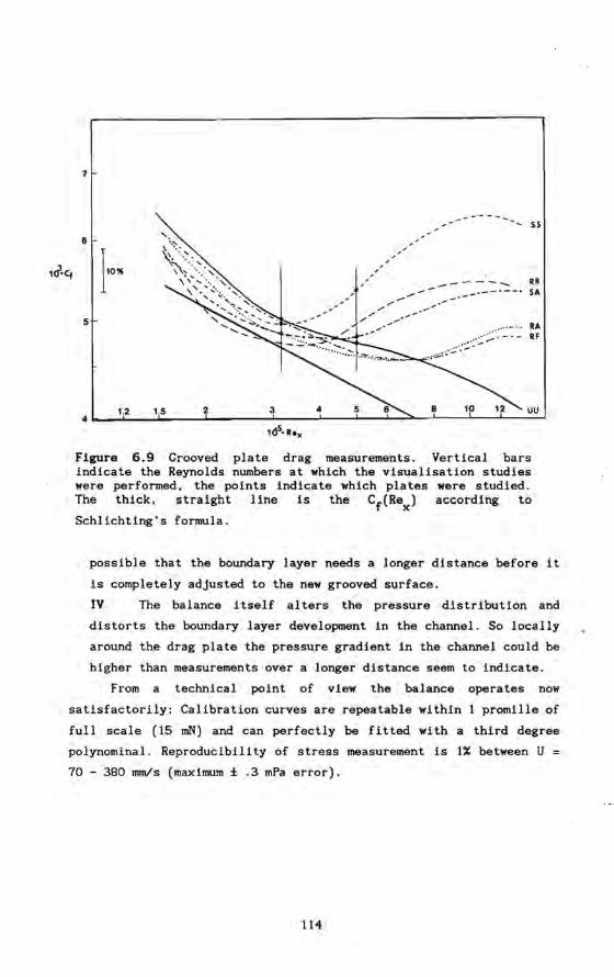
1 if· Cf

7

6

)'0% , , ,

5

"

------, SS

__ - - -........ RR • __ .--'--' SA

RA RF

4b-__ 1~,2~ __ 1~,5~ ____ ~2 _________ 3~ ____ ~4 ____ ~ __ ~ __ ~~~ __ ~ __ ~ ____ U_U~

Flgure 6.9 Grooved plate drag measurements. Vertical bars indicate the Reynolds numbers at which the visualisation studies were performed, the points indicate which plates were studied. The thick, straight !i ne is the Cf(Rex ) accordlng to

Schlichting's formula.

possible that the boundary layer needs a longer distance before it

is completely adjusted to the new grooved surface.

IV Ihe balance i tself alters the pressure distribution and

distorts the boundary layer development in the channel. So locally

around the drag plate the pressure gradient in the channel could be

higher than measurements'over a longer distance seem to indicate.

From a technica 1 point of view the balance operates now

satisfactorily: Calibration curves are repeatable within 1 promille of

ful! scale (15 mN) and can perfectly be fi tted with a third degree

polynominal. Reproduèibility of stress measurement is 1% between U = 70 - 380 mmls (maximum ± .3 mPa error).

114

Chapter 7 Discussion and suggestions for further research.

In the previous three chapters we presented the experimental

data collected so faro Now is the time to connect these data with the

theoretical ideas stated in chapter 2 and also with more speculative

ideas. Evaluating this we will try to point out .some areas of further

research.

Both the windtunnel measurements and the water channel point

'measurementsshow only marginal changes in the mean velocity profile.

A decrease in Reynolds shear stress (-uv) is observed at both

measurement sites and the amount is comparable with the reduction in

wall shear stress. The combination of both facts means that the

relation between velocity gradient and shear stress is affected (the

mixing length 2). which questions the very validity of the present

statistical turbulent models in this type of flow. Itis. however.

possible that the difference in veloei ty profiles imp lied by the

difference in shear stress profiles falls within the experimental

errors.

A decrease in u' is observed at all veloeities. the maximum of

u' is ca 10% lower. Significant changes in third order correlation ~

are observed. but the changes in the other quantities Vü2. uv2 and ~

are less pronounced and probably not statistically significant. The

first observation indicates a change in the ratio between shear stress

and turbulent kinetic energy a = -üV / (u' 2 + v· 2 ). This indicates

again a breakdown of the turbulent modelling. which of ten assumes that

a is constant. The measurements show also that on a spanwise grooved

wall the ratio a is largely unaffected. The fact that those changes

also occur at higher speed. outside the range of maximum drag

reduction. leads to the speculation that the observed effect on the

drag is the outcome of two opposing processes:

I The increased surface ·area of ribs penetrating the boundary

layer whichs tends to increase the drag.

11 The influence on the turbulent structures near the wall which

tends to inhibit the turbulent momentum exchange and thus lowers

the drag.

It also sustains

visualisation experiments

the assumption

which study

115

that the

particularly

outcome of the

the turbulent

structure near the wall (the second process), is not very sensitive to

the precise velocity of the flow.

The results of burst detection in the buffer layer are somewhat

ambiguous. Although some differences in burst frequency can be

detected it is questionable whether they are significant. Particularly

if one considers the potential influence of choosing a different

reference height or trigger level. The dependence on trigger level

which Is similar In all cases, leaves only two possible conclusions.

Either no changes occur in the boundary layer, or the method itself Is

not sensitlve to changes in turbulent structure. The last possibility

is reinforced by the observation that the shape of ave rage .vertical

velocity component during a burst over a spanwise grooved wall is

drastically changed without a very clear effect on the burst frequency

measured.

The study of the visual flow patterns did not indicate that

different turbulent structures exist above a longitudinal grooved

wall. In particular the low speed streaks are still visible. To the

naked eye some differences in the details of the turbulent structures

between smooth wall and longitudlnal grooved wall flow are also

visible but they are difficult to quantify. The following observations

apply :

I

11

The flow appears to be more chaotic.

Near the wall the bubble lines show small wiggles of the

spacing as the riblets, which are clearly caused by the

riblets.

III The apparent length of the low speed streaks is shorter.

same

IV It is observed that the low speed streaks are not attached to

the riblets, the minima clearly meander over the topsand

valleys.

When we try to summarize the visual differences between the

smooth wall flow and the transverse grooved wall flow, we note the

following points:

I The flow appears to be more regular.

11 The low speed streaks are more intense, the minima are lower.

The most obvious conclusions are:

I The longitudinal riblets hinder the formation of low speed

streaks, without completely inhibi ting U~em.

116

11 If there Is more wall shear stress low speed streaks bacome

more pronounced.

With LDA measurements, performed slmultaneously with

vlsuallsatlon we are able to investigate the relation between low

speed streaks and shear stress. rhe moments of large instantaneous

Reynolds shear stress cannot ba indentified wUh a single structure

visible in plan view, instead both in high speed regions and in low

speed streaks there can be a large amount of momentum transfer. No

simple clear connection appears between large toont and instantaneous

Reynolds shear stress as measured wi th LDA and the v isual ised low

speed streaks. This indicates that the momentum transport is

presumably a property of the complete set of structures and their

interactions in the lower part of the boundary layer and not of only a

single structure.

This is, however, not the complete story. Statistical analysis

shows some shift in distribution of structures seen at posi tions at

which Reynolds shear stress is extreme compared to the distribution at

random points. So in a statistical sense there is a connection but

this does not translate in a direct cause and effect relation. A more

direct clue is the observation that the vertical velocl ty in a low

speed streak on a grooved wall is nearly zero although this needs to

be confirmed by more elaborate measurements. This implies a lower

momentum transfer in such a streak.

As is noted in chapter 2 the current ideas are not adequate to

obtain a quantitative estimate of the amount of possible drag

reduction . The experiments indicate that only the flow in the buffer

layer and below is affected by the grooves. A model should concentrate

on phenomena which occur there: the change from momentum transfer by

viscous forces to turbulent ' exchange. The first stage of this process

is apparently the format ion of low speed streaks (and of course the

high speed regions in between) . An extension of the laminar flow

calculations (§2.2) with secondary flow could" give insight into the

flow but it will not predict drag reduction .

For practical purposes and perhaps also to provide more ideas

for the theor ies, an extension of the measurements to f lows wi th

different pressure gradients could ba helpful. Much could be learned

also by performing the experiments on a set of geometrically scaled

grooves over a range of Reynolds numbars as large as possible.

117

A different ideais the application of the theory of Perry ea

[1986]. They considered the turbulent boundary layer flow as composed

of wall attached structures. The size and frequency of these

structures follow certain sealing laws. Assuming the destruction of

those structures by the grooves the influence on the spectra and

velocity profiles can be estimated.

From the present thesis it is hopefully clear that the problem

of turbulent drag reduction is far from solved. This is not surprising

because turbulence itself is a subject which is barely understood. An

implication of this statement is that whichever experiment is

performed over a grooved wall. it should also be done on a smooth wall

as a reference. A second lesson. now that the simple ideas do not seem

to work properly. is that seriously more effort should be put in

developing a theory which has at least the potential to explain the

drag reduction.

118

Appendix A Tbe method of Head applied to the waterchannel flow.

Head's method to calculate the development of a turbulent

boundary layer is an integral method which uses three ordinary

differential equations to solve for the unknowns e (the momentum loss

thickness), H (the shape factor ö*/9) and Cf (the friction

coeff icient) .

The equations used are:

with empirically determined algebraic functions:

{ 0.8234

1.5501

(H - 1.1)-1.287 + 3.3 H ~ 1.6

(H - 0 . 6778)-3.064 + 3.3 H ~ 1.6

F = 0.0306 (H 1 - 3.0)-0.6169

which describe the entrainment of the boundary layer.

Von Karman's equation:

de 9 dU 1 dx + (2 + H) ij a;c<" = 2" Cf

co

and the Cf law given by Ludwieg and Tillmann [1949]:

Cf = 0 . 246 10-0 . 678 H R -0.268 • ee

In order to predict the pressure gradient too, we extend the

system by an equation which describes the conservation of mass flowing

through a channel with constant width wand height h :

~ [ Uco (w - 2 H 9) (h - H 9) ] = 0

119

The interaction between the side wall boundary layers and the

bottom boundary layer is not taken into account in this equation.

Nevertheless 1f a « wand e « h the accuracy of this equation is

acceptable.

Ihis set of equations can be used with any standard method to

solve a set of ordinary differential equations to obtain aprediction

of the boundary layer development.

120

Appendix B Accuracy of the spanwise velocity correlation.

In §5.4 is explained how 500 instanteneous spanwise velocity

profiles are used to estimate the correlatlon function. A previous

experiment using 2000 profiles and also physical intuition indicated

that 500 profiles is areasonabie amount to obtain an accurate

estimate of the correlation function and the other quantities of

interest.

Such an experlmental result, however, is always obscured by

unknown influences like a possible drift in velocity • a change in

lighting and various other circumstances. A mathematical and

statistical analysis to determine the minimum number of profiles

needed for our purpose yields very unwieldy formuias . Therefore an

additional numerical simulàtion was made.

We proceed in two steps. First a large number (2000) artificial

velocity profiles must be generated. These profiles must mimic the

statistical properties of the natural velocity profiles. Secondly we

derive the statistical quantities we are interested in, from different

sets of velocity profiles.

The creation of the artificial velocity profiles is done in

several steps: We generate a sequence xi (i = 1. .100000) of random

numbers between -0.5 and 0.5 and pass it through a digital filter,

giving a new sequence Yi . Inspecting the experimental results it was

determined that a satisfactorily approximation of the real correlation

function can be obtained using a damped, oscillating impulse response

h(z) for the filter. A general formuia for this Is:

h(z) -az e sin(boz)

The advantage of this formula is that it . has a simple z-transform

whlch can he used to calculate the digital filter constants needed.

The actual transformation is .done uslng the formula:

121

Yi = al x1- 1 - bI Yl-1 - b2 Yi - 2 -a

sin(b) al = e

bI = 2 e -a

cos(b)

b2 = e -2a

It is only fair to note that experiments lndicate that

correlations functions measured in turbulent flows have a slower than

exponential decay [see eg Hinze 1972]. This means that the numerical

experiment can give a somewhat more optimistic view than really

warranted. But a non-exponentially decaying function has no simple

z-transform and compllcates the mathematlcs.

The procedure described here leads to a sequence Yl with a zero

mean and a rms value cr of y

and a correlatlon function ~ (z) of yy

~ (z) yy

cr; e -az [ cos(bz) + !b sin(bz) ]

The actual values used for a and b are: a = 0.18 and b = 0 . 25. These

va lues are such that we obtain a correlation function of the correct

width (first zero point at 10) and with a first minimum of a depth of

.1. The generated sequence Yi (i= 1 .. 100000) has a rms value of 0.275.

the theoretical correct value is 0 .2760. The agreement is

satisfactorily. The numbers of the sequence Yi are multiplied by 25.

and incremented with 50. to put them in the range of the numbers from

the actual experiments. Next. the resul ting numbers are rounded and

stored on disk in 2000 groups of 50. just as the sequences from the

experiments are stored. The sequences generated in this way mimic the

behaviour of the proflles stored in the water channel experiments.

With the computer programsused in the actual experiment we can

now extract the statistical quantities. We present the results of this

exercise in Table B.la-d. Table B.la displays the numbers as they

122

theoretically should beo The columns show from left to right the

position along the wire (the z-coordinate). the ave rage velocity. the

rms value of the velocity. the correlation function and an estimate of

the variance of the correlation function. Table B.lc gives the numbers

derived from the 500 artificial profiles together with an estimate of

the variance of the correlation (5th column). The variance in the rms

value of the velocity is about 5%. The width and the depth of the

Brst minimum of the correlation function are reproduced wi th an

accuracy of 1% and 10% respectively. The deviations from the

theoretical curve are in line with the estimate of the variance which

is provided.

The numerical experiment also indicates that the averaging over

125 profiles (tabIe B.lb) can lead to an error of 30% in the dep th of

the first minimum. This would be unacceptably high for our purposes.

The averaging over 2000 profiles (tabie B.ld) leads of course to more

accurate results. The increase in accuracy is. however. only marginal.

The conclusion is that under ideal circumstances 500 velocity

profiles are enough to reconstruct the correlation function with an

accuracy suited to our demands.

123

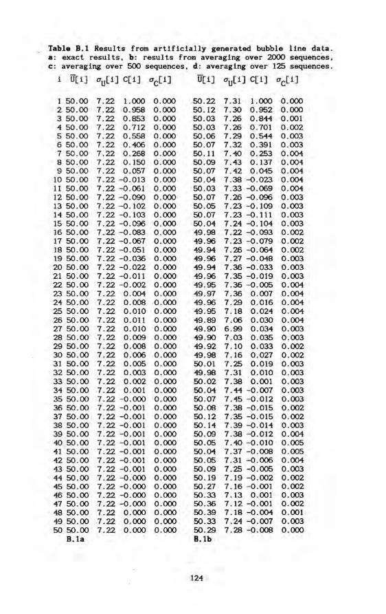
Tabla B.1 Results from artificially generated bubble line data. a: exact results. b: results from averaging over 2000 sequences. c: averaging over 500 sequences, d: averaging over 125 sequences.

1 50.00 7.22 1.000 0.000 2 50.00 7.22 0.958 0.000 3 50.00 7.22 0.853 0.000 4 50.00 7.22 0.712 0.000 5 50.00 7.22 0.558 0.000 6 50.00 7.22 0.406 0.000 7 50.00 7.22 0.268 0.000 850.00 7.22 0.150 0.000 9 50.00 7.22 0.057 0.000

10 50.00 7.22 -0.013 0.000 11 50.00 7.22 -0.061 0.000 12 50.00 7.22 -0.090 0.000 13 50.00 7.22 -0.102 0.000 1450.00 7.22 -0.103 0.000 15 50.00 7.22 -0.096 0.000 16 50.00 7.22 -0.083 0.000 17 50.00 7.22 -0.067 0.000 18 50.00 7.22 -0.051 0.000 19 50.00 7.22 -0.036 0.000 20 50.00 7.22 -0.022 0.000 21 50.00 7.22 -0.011 0.000 22 50.00 7.22 -0.002 0.000 23 50.00 7.22 0.004 0.000 24 50.00 7.22 0.008 0.000 25 50.00 7.22 0.010 0.000 26 50.00 7.22 0.011 0.000 27 50.00 7.22 0.010 0.000 28 50.00 7.22 0.009 0.000 29 50.00 7.22 0.008 0.000 30 50.00 7.22 0.006 0.000 31 50.00 7.22 0.005 0.000 32 50.00 7.22 0.003 0.000 33 50.00 7.22 0.002 0.000 34 50.00 7.22 0.001 0.000 35 50.00 7.22 -0.000 0.000 36 50.00 7.22 -0.001 0.000 37 50.00 7.22 -0.001 0.000 38 50.00 7.22 -0.001 0.000 39 50.00 7.22 -0.001 0.000 40 50.00 7.22 -0.001 0.000 41 50.00 7.22 -0.001 0.000 42 50.00 7.22 -0.001 0.000 43 50.00 7.22 -0.001 0.000 44 50.00 7.22 -0.000 0.000 45 50.00 7.22 -0.000 0.000 46 50.00 7.22 -0.000 0.000 47 50.00 7.22 -0.000 0.000 48 50.00 7.22 0.000 0.000 49 50.00 7.22 0.000 0.000 50 50.00 7.22 0.000 0.000

B.1a

50.22 7.31 1.000 0.000 50.12 7.30 0.952 0.000 50.03 7.26 0.844 0.001 50.03 7.26 0.701 0.002 50.06 7.29 0.544 0.003 50.07 7.32 0.391 0.003 50.11 7.40 0.253 0.004 50.09 7.43 0.137 0.004 50.07 7.42 0.045 0.004 50.04 7.38 -0.023 0.004 50.03 7.33 -0.069 0.004 50.07 7.26 -0.096 0.003 50.05 7.23 -0.109 0.003 50.07 7.23 -0.111 0.003 50.04 7.24 -0.104 0.003 49.98 7.22 -0.093 0.002 49.96 7.23 -0.079 0.002 49.94 7.26 -0.064 0.002 49.96 7.27 -0.048 0.003 49.94 7.36 -0.033 0.003 49.96 7.35 -0.019 0.003 49.95 7.36 -0.005 0.004 49.97 7.36 0.007 0.004 49.96 7.29 0.016 0.004 49.95 7.18 0.024 0.004 49.89 7.06 0.030 0.004 49.90 6.99 0.034 0.003 49.90 7.03 0.035 0.003 49.92 7.10 0.033 0.002 49.98 7.16 0.027 0.002 50.01 7.25 0.019 0.003 49.98 7.31 0.010 0.003 50.02 7.38 0.001 0.003 50.04 7.44 -0.007 0.003 50.07 7.45 -0.012 0.003 50.08 7.38 -0.015 0.002 50.12 7.35 -0.015 0.002 50.14 7.39 -0.014 0.003 50.09 7.38 -0.012 0.004 50.05 7.40 -0.010 0.005 50.04 7.37 -0.008 0.005 50.05 7.31 -0.006 0.004 50.09 7.25 -0.005 0.003 50.19 7.19 -0.002 0.002 50.27 7.16 -0.001 0.002 50.33 7.13 0.001 0.003 50.36 7.12 -0.001 0.002 50.39 7.18 -0.004 0.001 50.33 7.24 -0.007 0.003 50.29 7.28 -0;008 0.000 B.lb

124

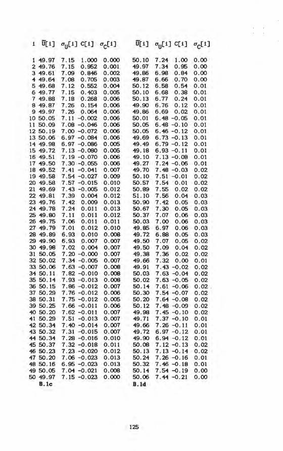
i rr[i] uu[1] Cri] uc[1] rr[i] uU[i] cri] uc[1]

1 49.97 7.15 1.000 0.000 50.10 7.24 1.00 0.00 2 49.76 7.15 0.952 0.001 49.97 7.34 0.95 0.00 3 49.61 7.09 0.846 0.002 49.86 6.98 0.84 0.00 4 49.64 7.08 0.705 0.003 49.87 6.66 0.70 0.00 5 49.68 7.12 0.552 0.004 50.12 6.58 0.54 0.01 6 49.77 7.15 0.403 0.005 50.10 6.68 0.38 0.01 7 49.88 7.18 0.268 0.006 50.13 6.77 0.24 0.01 8 49.87 7.26 0.154 0.006 49.90 6.76 0.12 0.01 9 49.97 7.26 0.064 0.006 49.86 6.69 0.02 0.01

10 50.05 7.11 -0.002 0.006 50.01 6.48 -0.05 0.01 11 50.09 7.08 -0.046 0.006 50.05 6.48 -0 . 10 0.01 12 50.19 7.00 -0.072 0.006 50.05 6.46 -0 . 12 0 .01 13 50.06 6.97 -0.084 0.006 49.69 6.73 -0.13 0.01 14 49.98 6.97 -0.086 0.005 49.49 6.79 -0.12 0.01 15 49.72 7.13 -0.080 0.005 49.18 6.93 -0.11 0.01 16 49.51 7.19 -0.070 0.006 49.10 7.13 -0.08 0.01 17 49.50 7.30 -0.055 0.006 49.27 7.24 -0.06 0 .01 18 49.52 7.41 -0.041 0.007 '19.70 7.48 -0.03 0.02 19 49.58 7.54 -0.027 0.009 50.10 7.51 -0.01 0.02 20 49.58 7.57 -0.015 0.010 50.57 7.54 0.01 0.02 21 49.69 7.-43 -0.005 0.012 50.89 7.55 0.02 0.02 22 49.81 7.39 0.004 0.012 51.10 7.56 0.04 0.03 23 49.76 7.42 0.009 0.013 50.90 7.42 0.05 0 .03 24 49.78 7.24 0.011 0.013 50.67 7.30 0.05 0.03 25 49.80 7.11 0.011 0.012 50.37 7.07 0.06 0.03 26 '19.75 7.06 0.011 0.011 50.03 7.00 0.06 0.03 27 49.79 7.01 0.012 0.010 '19.85 6.97 0.06 0.03 28 49.89 6.93 0.010 0.008 49.72 6.88 0.05 0.03 29 49.90 6.93 0.007 0.007 49.50 7.07 0.05 0.02 30 49.98 7.02 0.004 0.007 49.50 7.09 0.04 0 . 02 31 50.05 7.20 -0.000 0.007 '19.38 7.36 0.02 0.02 32 50.02 7.34 -0.005 0.007 49.66 7.32 0.00 0.01 3350.06 7.63 -0.007 0.008 49.91 7.43 -0.02 0.02 34 50.11 7.82 -0.010 0.008 50.03 7.63 -0.04 0.02 3550.14 7 .93 -0.013 0.008 50 .02 7.63 -0.05 0.02 36 50.15 7.86-0.012 0.007 50.14 7.61 -0.06 0.02 . 37 50.29 7.76 -0.012 0.006 50.30 7.54 -0.07 0 .02 38 50.31 7.75 -0.012 0.005 50.20 7.64 -0.08 0.02 39 50.25 7.66 -0.011 0.006 50.12 7.48 -0.09 0.02 40 50.20 7.62 -0.011 0.007 49.98 7 .45 -0.10 0 .02 41 50.29 7.51 -0.013 0.007 49.71 7.37 -0.10 0.01 42 50.34 7.40 -0.014 0.007 '19.66 7.26 -0.11 0.01 43 50.32 7.31 -0.015 0.007 49.72 6.97 -0.12 0.01 44 50.34 7.28 -0.016 0.010 49.90 6.94 -0.12 0.01 45 50.37 7.32 -0.018 0.011 50 .08 7 . 12 -0.13 0.02 4650.23 7.23 -0.020 0.012 50.13 7.13 -0.14 0.02 47 50.20 7.06 -0.023 0.013 50.24 7.26 -0.16 0.01 48 50.16 6.95 -0.023 0.013 50.32 7.46 -0.18 0.01 49 50.05 7.04 -0.021 0.008 50.14 7.54 -0.19 0.00 50 '19.97 7.15 -0.023 0.000 50.06 7.44 -0.21 0 .00

B.lc B.ld

125

References

M.S. ACARLAR & C.R. SMITH 1987 A study ·of hairpin vortices in a laminar boundary layer. Part 1. Hairpin vortices generated by a hemisphere protuberance . J. Fluid Mech. 175 pl .

M.S. ACARLAR & C.R. SMITH 1987 A study of hairpin vortices in a laminar boundary layer . Part 2. Hairpin vortices generated by fluid injection. J. Fluid Mech. 175 P43 .1

M. ACHARYA, J. BORNSTE IN, M. P. ESCUIj> I ER & V. VOKURKA 1985 Development of a floating element balan?e for the measurement of surface shear stress. AlAA Journal Vol. 123, 3 p410.

P.H. ALFREDSSON & A.V. JOHANSSON. 198~ Timescales in turbulent channel flow. Phys. Fluids 27 p1974. I

1

P. BANDYOPADHYAY & A.K.M . F. HUSSAIN. 19Ss The universal nature of zero-crossing time and veloei ty scales i!n turbulent shear f lows. AlAA Journal 23 p161.

D.W. BECHERT, G. HOPPE & W.E. REIF 1985 On the drag reduction of the shark skin. AlAA Shear flow Cont ol Conference, Boulder, Colorado.

D. W . BECHERT, M BARTENWERFER, G. HOPP & W. E. RE I F 1986 Drag reduction mechanisms derived from sh rk skin 15th Congress, International council of the aeronautic~l sciences, London.

B. VAN DEN BERG 1986 Drag reduction I potentialof turbulence manipulation in adverse pressure gradient flows. NLR MP B6060 U

R. F. BLACKWELDER & R.E. KAPLAN. 1976 l the wal! structure of turbulent boundary layer. J~ Fluid Mech.1 Vol 16, part 1, 1976 p89

R. BLOKLAND & K. KRISHNA PRASAD. 1986 Jome visualisation studies on turbulent boundary layers using oLl tiwire hydrogen bubble generation. AGARD-CPP-413, p28-1. I

D.C. BOGARD & W.G. TIEDERMAN 1986 Burst detectlon with single-point velocity measurements J.FIJid Mech. 162 p389

E.F. BRADLEY 1968 A shearing stress meter for micrometorologlcal studies. Quart. J. R. Met. Soc . 94 p3BO

D. M. BUSHNELL 1985 Turbulent drag reduction for external flows. ACARD Rep. 723, p55-1.

D. M. BUSHNELL, J.M. HEFNER & R.L. ASH 1977 Effects of compliant wall motion on turbulent boundary layers. Physics of Fluids vol 20,no 10, part I I. pS3!.

126

B.J. CANTWELL 1981 Organized motion in turbulent flow. Ann Rev Fluid Mech. p457-515 .

T. CEBECI & P. BRADSHAW 1977 Momentum transfer in boundary layers. McGraw-Hill 1977.

W. VAN DAM 1986 Weerstandsvennindering grenslaag als gevolg van microgroeven. University of Technology. afstudeerverslag.

in een turbulente (In dutch) Delft.

L. DJENIDI. F. ANSELMET & L. FULACHIER 1987 Influence of a riblet wall on boundary layers. Proceedings International Conference on Turbulent Drag Reduction. Ro. Aer. Soc. London. To be published.

J. DOUGLAS McLEAN. D. N. GEORGE-FALVY. P.P. SULLIVAN 1987 Flight-Test of Turbulent Skin-Friction Reduction by Riblets. Proceedings International Conference on Turbulent Drag Reduction. Ro. Aer. Soc. London. To be published.

E.R. VAN DRIEST 1956 On turbulent flow near a wall. Journalof Atmospherlc Sciences 23.

J. P. ECKMANN 1981 Roads to turbulence in dissipative dynamical systems. Rev. Mod. Phys. 53. p643.

H.A. EINSTEIN & H. LI 1956 The viscous sublayer along a smooth boundary. J. Eng. Mach. Div. Am. Soc. Civ. Engrs. vol 82 (EM2). p945.

R.E. FALCO 1983 New results. a review and synthesis of the mechanism of turbulence production in boundary layers and i ts modification. AIAA 21st Aerospace Sclences Meeting Reno. Nevada.

J.A. GALLAGHER & A.S.W. THOMAS 1984 Turbulent boundary layer characteristics over streamwise grooves. AIAA paper No. 84-2185.

A. J. GRASS. 1971 Structural features of turbulent flow over smooth and rough boundaries. J. Fluid Mech. 50 p233.

M.R. HEAO 1958 Entrainment in the turbulent boundary layer. Aer. Res. Council R&M 3152

J.N. HEFNER. J.B. ANDERS. "D.M. BUSHNELL 1983. Alteration of outer flow structures for turbulent drag reduction. AIAA 21st Aerospace Sciences Meeting. Reno. Nevada.

J.O. HINZE 1975 Turbulence. Mc Graw HilI.

D. HOOSHMAND. R. YOUNGS & J.M WALLACE 1983. An experimental study of changes in the structure of a turbulent boundary layer due to surface geometry changes AIAA 21th Aerospace Sciences Meeting. Reno. Nevada.

F. HOWARD.L. WEINSTEIN.D. BUSHNELL 1981 Longitudinal grooves for bluff body drag reductlon. AIAA Journal 19. p535.

127

P.S. JANG, D.J. BENNEY & R.L. GRAN 1986 On the origiIi of streamwise vortices in a turbulent boundary layer. J . Fluid Mech. 169 p109.

J. B. JOHANSEN & C.R. SMITH. 1986 The effects of cylindrical surfacemodifications on turbulent layers. AIAA Journal 24 p10B1

A.V . JOHANSSON, J . HER & J.H. HARITONIDIS 1987 On the generation of high-amplitude wall-pressure peaks in turbulent boundary layers and spots. J.Fluid Mech. 175 p119

Th. VON KARMAN 1931 Mechanische Ahnlichkeit und Turbulenz. NACA TM611.

J.H.A. KERN 1985 Meting van de turbulente schuifspanning met een laser doppier anemometer in de grens laag boven een vlakke en een ruwe wand. Afstudeerverslag TH Eindhoven R-710-A

J. KIM, P. MOIN & R. MOSER 1987 Turbulence statistics in fully developed channel flow at low Reynolds number. J. Fluid Mech. 177 p133.

S. J. KL! NE, W. C. REYNOLDS, F. A. SCHRAUB & P. W. RUNDST ADLER. 1967 The structure of turbulent boundary layers. J. Fluid Mech. 30 pH1.

A.N. KOLMOGOROV. 1941 The local structure of turbulence in incompressible flow for very large Reynolds number. Compt. rend. acad. sci. U. R. S. S., 30, p31.

P. KR ISCHKER & Th. GAST. 1982 Induktiver Differential

Querankergeber hoher Aufl~sung. Technisches Mess 49. Jahrgang Heft 2 p43 .

J .M.G. KUNEN 19B4 On the detection of coherent structures in turbulent flows. Doctoral thesis, Delft University of Technology.

J. LEMA y, D. PROVENCAL , R. GOURDEAU, V. D. NGUYEN & J. 0 I Cl< I NSON 1985 More detailed measurements behind turbulence manipulators including tandem devices using servo-controlled balances. AlAA Shear flow control conference Boulder, Colorado.

C.K . LIU, S.J. KLINE & J.P. JOHNSTON . 1966 An experimental study of turbulent boundary layers on rough wal Is. Report MD-15 Thermosciences Division, Department of Mechanical Engineering, Stanfort University. Stanfort, California.

L.J. LU & C.R. SMITH. 1985 Image processing of hydrogen bubble flow visualisation for determination of turbulent statistics and bursting characieristics . Exp. in Fluids 3 p 349.

T .S. LUCHIK & W.G. TlEDERMAN 1987 Timescale and structure of ejections and bursts in turbulent channel flows. J.Fluid Mech.114 p529.

128

H. LUDWIEC & W. TILLMANN 1949 Untersuchungen Wandschubspannung in turbulenten Reibungsschichten. vol 17, p288.

~ber die ing.-Arch. ,

N.K.MADAVAN, S. DUETCH & C.L. MERKLE 1985 Measurernents of local skin friction in a microbubble-modified turbulent boundary layer. j. Fluid Mech. 156, p237.

j.C. MUMFORD & A.M. SAVILL 1984 Parametric studies of flat plate, turbulence manipulators including direct drag results and laser flow visualisation. ASME Fluid Engineering Division Vol 11 p41.

H. NAKACAWA & I. NEZU. 1981 Structure of space-time correlations of bursting phenomena in an open-channel flow. j. Fluid Mech. 104 plo

P. N ITSCHKE 1984 tubulent flow in

Thesis smooth

Experimental investigation and longitudinal grooved

of the tubes.

Max-Planck-Institute f~r Str~mingsforschung, Coettingen (West Cermany). Fachinformationszentrum, Karlsruhe, West Cermany

G. R. OFFEN & S. j. KUNE 1973 Experiments on the velocity characteristics of bursts and on the interaction between the inner and outer regions of a turbulent boundary layer. Rep. no. MD-31 Stanford University, Stanford, California.

A.G. PAPATHANASIOU & R. T. NAGEL 1986 Boundary layer control by acoustic excitation. AlAA 10th Aeroacoutics Conference Seattle, Washington.

S .. V. PATANKAR 1980 Numerical Heat Transfer and Fluid Flow. Hemisphere Pub.

A.E. PERRY, S. HENBEST & M.S. CHONG. 1986 A theoretica I and experimental study of wall turbulence. j. Fluid Mech. 165 p163.

L. PRANDTL 1925 Bericht ~ber untersuchungen zur ausgebildeten Turbulenz, Z. angew.Math. und Mech., Vol 5, p136.

O. REYNOLDS 1895 On the dyriamical theory of · incompressible viscous fluid and the determination of the criterium. Philos. Trans. R. Soc. London, Ser. A, 186 p123.

W.-E. REIF & A. DINKELACKER 1982 Hydrodynamics of the squamation

in fast swiuming sharks. Neues jahrbuch f~r Palaeontologie. Abhandlungen Band 164, Schweizerbart'sche Verlagsbuchhandlung.

Geologie p184.

und E.

j. ROTTA 1972 Turbulent boundary layers in incompressible flow. Progress in Aer. Sc. Vol 2.

129

A.M. SAVILL 1986 Effects on turbulent boundary layer structure of I ongitudinaI riblets alone and in combination with outer Iayer devices . Proc. 4th. Int. Symp. on Flow Visuallsation. Paris. Hemisphere Pub. Corp .. Washington.

A.M SAVILL. T.V. TRUONG & I.L. RYHMING 1987 Turbulent drag reduction by passive means. IMHEF. Ecole Polytechnique Federale de Lausanne Report T-87-3

W. G. SAWYER & K. G. WINTER 1987 An Investigation of the Effect on Turbulent Skin Friction of Surfaces with Streamwise Grooves . Proceedings International Conference on Turbulent Drag Reduction. Ro. Aer. Soc. London. To be published.

H. SCHLICHTING 1979 Boundary layer theory. McGraw-Hill

C.R. SMITH & S.P. SCHWARTZ 1983 Observation of streamwlse rotation in the near-wall region of a turbulent boundary layer. Phys. Fluids. Vol 26. p3.

D. SPALDING & N. AFGAN 1977 Heat transfer and turbulent buoyant convection. Vol I. p 339. Hemisphere Publishing Corporation. Washington.

]. VAN DER STEEG 1983 De turbulente grenslaag op een flexibel oppervlak. Afstudeerverslag TH Delft MEAH 22.

A.A. TOWNSEND 1976 The structure of turbulent shear flow. Second ed. Cambridge Universlty Press.

T. UTAMI & T UENO 1987 Experimental study on the coherent structure of turbulent opeL channel flow using vlsualisation and picture processing. ].Fluid Mech. 174 p399

P. S. VIRK 1971 An elastic sublayer model for drag reduction by dilute solutions of linear macromolecules . ]. Fluid Mech. 45 p417.

P.S. VIRK 1971 Drag reduction in rough pipes. ] . Fluid Mech. 45 p220.

M.]. WALSH 1982 Riblets as a viscous drag reduction technique. American Insti tute of Aeronautics and Astronautics . Aerospace Sciences Meeting. 20th. Orlando. FL. Jan . 11-14. AlAA paper 82-0169.

M.]. WALSH & A.M. LINDEMANN. 1984 Optimization and application of riblets for turbulent drag reduction. AIAA paper 84-0347

130

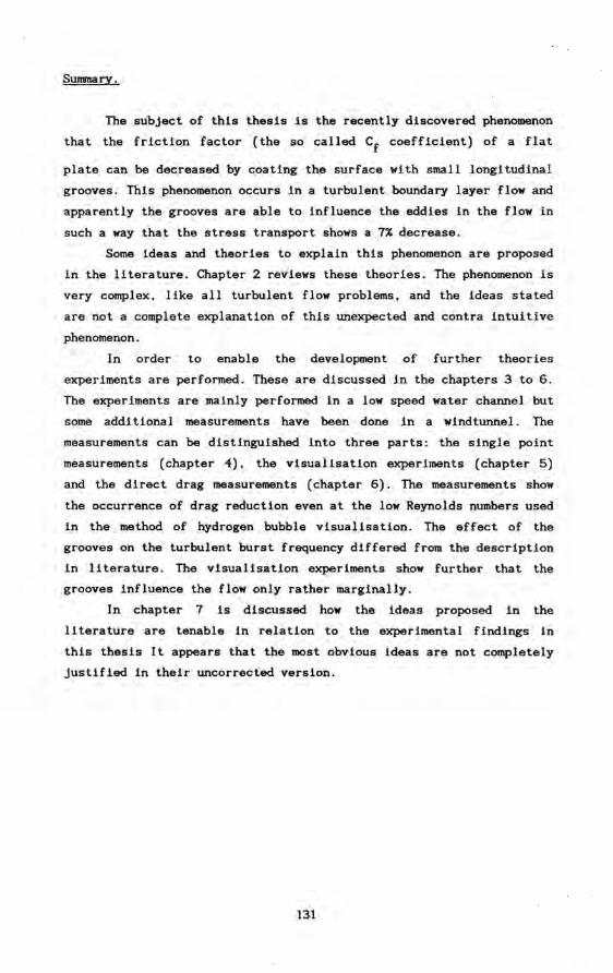
Sunmary.

The subject of this thesis is the recently discovered phenomenon

that the friction factor (the so called Cf coeffic1ent) of a flat

plate can be decreased by coating the surface with small longitudinaI

grooves. This phenomenon occurs in a turbulent boundary layer flow and

apparently the grooves are able to influence the eddies in the flow in

such a way that the stress transport shows a 7% decrease.

Some. ideas and theories to explain this phenomenon are proposed

in the literature. Chapter 2 reviews these theories. The phenomenon is

very complex, like all turbulent flow problems, and the ideas stated

are not a complete explanation of thls unexpected and contra intuitive

phenomenon.

In order to enable the development of further theories

experiments are performed. These are discussed in the chapters 3 to 6.

The experiments are mainly performed in a low speed water channel but

some addi tional measurements have been done in a windtunnel. The

measurements can be distinguished into th ree parts: the single point

measurements (chapter 4), the visua11sation experiments (chapter 5)

and the direct drag measurements (chapter 6). The measurements show

the occurrence of drag reduction even at the low Reynolds numbers used

in the method of hydrogen bubble visua11sation. The effect of the

grooves on the turbulent burst frequency differed from the description

in 11terature. The visua11sation experiments show further that the

grooves influence the flow only ,rather marginally.

In chapter 7 is discussed how the ideas proposed in the

11 terature are tenable in relation to the experimental findings in

this thesis It appears that the most obvious ideas are not completely

justified in their uncorrected version.

131

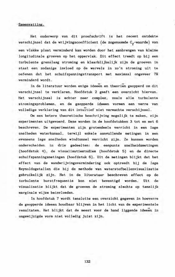
"Samenvatting.

Het onderwerp van dit proefschrift is het recent ontdekte

verschijnsel dat de wrijvingscoefficient (de zogenaamde Cf-waarde) van

een vlakke plaat verminderd kan worden door het aanbrengen van kleine

longitudinale groeven op het oppervlak. Dit effect treedt op bij een

turbulente grens laag stroming en klaarblijkelijk zijn de groeven in

staat een zodanige invloed op de wervels in zo'n stroming uit te

oefenen dat het schuifspanningstransport met maximaal ongeveer 7%

verminderd wordt.

In de literatuur worden enige idee~n en theori~n geopperd om dit

verschijnsel te verklaren. Hoofdstuk 2 geeft een overzicht hiervan.

Het verschijnsel is echter zeer complex, zoals alle turbulente

stromingsproblemen, en de geopperde idee en vormen een verre van

volledige verklaring van dit intuïtief niet verwachte verschijnsel.

Om een betere theoretische beschrijving mogelijk te maken, zijn

experimenten uitgevoerd. Deze worden in de hoofdstukken 3 tot en met 6

beschreven. De experimenten zijn grotendeels verricht in een lage

snelheden waterkanaal, terwijl enkele aanvullende metingen in een

eveneens lage snelheden windtunnel verricht zijn. Ze kunnen worden

onderscheiden in drie gedeelten : de eenpunts snelheidsmetingen

(hoofdstuk 4) , de visualisatiestudies (hoofdstuk 5) en de directe

schuifspanningsmetingen (hoofdstuk 6). Uit de metingen blijkt dat het

effect van de wandwrijvingsvermindering ook optreedt bij de lage

Reynoldsgetallen die bij de methode van waterstofbellenvisualisatie

gebruikelijk zijn. Het in de literatuur beschreven effect op de

turbulente burstfrequentie kon niet bevestigd worden. Uit de

visualisatie blijkt dat "de groeven de stroming slechts op tamelijk

marginale wijze beinvloeden.

In hoofdstuk 7 wordt tenslotte een overzicht gegeven in hoeverre

de geopperde ideeen houdbaar blijven in het licht van de experimentele

resultaten. Het blij~t dat de meest voor de hand liggende idee~n in

ongewijzigde vorm niet volledig juist zijn.

132

Dankwoord.

Dit proefschrift was nooit tot stand gekomen zonder de hulp van

velen.

Zonder de inzet van drs. A. Koppius. dr. K. Prasad en ing. C.

Nieuwveldt was het project Dragreductie van het STW nooit ontstaan.

Ook de inzet en het enthousiasme van prof. dr. ir. G.Ooms. en zijn

bereidheid dit werk tot het einde toe te blijven begeleiden stemmen

mij tot dankbaarheid.

Ook alle leden van de werkeenheid Turbulentie hebben veel bijge­

dragen. Met name de inzet van ]. Stouthart bij het ontwerp en gebruik

van de balans is onmisbaar geweest. Uiteraard zou deze zonder de hulp

en het meedenken van mensen op de diverse werkplaatsen van de TU niet

tot stand zijn gekomen.

De samenwerking met de TU Delft in de personen van prof. dr. F.

Nieuwstadt. ir. H. Leijdens. W. van Dam. F Verhey is altijd plezierig

verlopen en heeft zeker bijgedragen aan de opzet van dit proefschrift

te verbreden.

Verder ben ik erkentelijk voor de bijdragen en inspanningen van

de studenten van de TU Eindhoven (in chronologische volgorde) H. Smol­

ders. ]. Kern. T. Gielen. C. Lamers en C. Delhez.

Curriculum Vitae.

3 januari 1959 Geboren in Eindhoven.

17 juni 1977 Diploma Gymnasium ~.

23 maart 1983 TH Eindhoven; diploma Technische Natuurkunde.

20 april 1983 - Wetenschappelijk assistent bij Technische 14 juli 1983 Hogeschool Eindhoven.

15 juli 1983 -15 juli 1987

1 sept 1987

In dienst bij STW/FOM. voor project Drag reduction. Werkzaam aan TU Eindhoven bij de vakgroep Transportfysica

Werkzaam als wetenschappelijk medewerker bij het VEG-Gasinstituut te Apeldoorn.

1~

Stellingen.

Behorende bij het proefschrift van

C.J.A. Pulles

Eindhoven , 4 maart 1988.

1 Het aantonen van verschillen in turbulente grenslagen boven een

gladde en boven wrijvingsverminderende oppervlakken is slechts zinvol

als er een relatie met het schuifspanningstransport gelegd wordt .

Dit proefschri ft .

2 Het optreden van wrijvingsvermindering in turbulente grens lagen

maakt de beperkingen van de huidige, .op statist i sche sluitingsrelaties

gebaseerde turbulente modellen duidelijk .

Di t proefschrift .

3 Het meten van burstfrequenties als indicatie voor kleine verschillen

in schuifspanningstransport is alleen dan zinvol wanneer meer bekend

is over de. relatie tussen burstfrequenti e , schuifspanning, detekt i eni­

veau's en effectieve meethoogte boven een ruwe wand .

J .M.G. Kunen (1984) , On the detection of coherent structures i n turbu­

l.ent. fl.OlDS . Thesis . Del.ft University Press .

Dit proefschrift.

4 Het ontbreken van een fundamentele theorie over turbulentie vermin­

dert de waarde van indirecte methoden ter bepaling van de wandwrij­

ving, met gebruik van empirisch bepaalde grootheden ten zeerste.

Dit proefschrift.

5 Voor het meten van instantaan schuifspanningstransport in een turbu­

lente grenslaag beperkt men zich meestal tot de Reynoldse schuifspan­

ningscomponent. Maar met name dicht boven wrijvingsreducerende opper­

vlakken zijn de resterende visceuze krachten een belangrijke parameter

J.M.. Wallace, J. BaUnt B P. VuJwslauceuic 1987 On the mechanisllt of

uiscous drag Reduction using streamwise aligned riblets: a reuiew with

some new results. Proc. Int. Conf. on Turb. Drag Reduction by Passiue

Means ., Roy. Aer. Soc., London.

6 Om te kunnen beslissen welke metingen goed zijn en welke niet

gebruikt een onderzoeker vooroordelen over het verschijnsel dat hij

onderzoekt. Met andere woorden metingen worden gebruikt ter

bevestiging van eigen en andermans vooroordelen.

N. Cartwright 1983 How the lQlOS of physics Ue. CLarendon Press,

Oxford.

7 Het gebruik van een waterkanaal in plaats van een windtunnel bij

experimenten met turbulente grenslagen is alleen dan te overwegen als

er voldoende tijd is. De factor honderd verschil in noodzakelijke

meettijd maakt een stage met waterkanaal experimenten voor de huidige

twee fasen studenten niet aantrekkelijk.

8 Als de groeven op haaienhuiden inderdaad de functie hebben de wrij­

vingsweerstand te verminderen, dan verdient het overweging schilvers

van geschikte afmetingen te mengen in de verf waarmee schepen geschil­

derd worden. Door slijtage van de verflaag kunnen dan de

wrijvingsverminderende groeven ontstaan.

J.S. Letcher Jr., J.K. Marchall, J.C. Oltuer 111 & N. Saluesen (1987)

Stars & Strtpes, Sctenttftc Amertcan August '87.

9 Experimenteel gezien gaat door drie punten altijd een rechte lijn.

Euclides 300 u C, ELementen.