ttsai/publications/gustafson-nakanishi-tsai-cmp10.… · Digital Object Identiﬁer (DOI) 10.1007/s00220-010-1116-6 Commun. Math. Phys. 300, 205–242 (2010) Communications in Mathematical

Digital Object Identifier (DOI) 10.1007/s00220-010-1116-6Commun. Math. Phys. 300, 205–242 (2010) Communications in

MathematicalPhysics

Asymptotic Stability, Concentration, and Oscillationin Harmonic Map Heat-Flow, Landau-Lifshitz,and Schrödinger Maps on R

2

Stephen Gustafson1, Kenji Nakanishi2, Tai-Peng Tsai1

1 Department of Mathematics, University of British Columbia, Vancouver, BC V6T 1Z2, Canada.E-mail: [email protected]; [email protected]

2 Department of Mathematics, Kyoto University, Kyoto 606-8502, Japan. E-mail: [email protected]

Received: 5 October 2009 / Accepted: 24 May 2010Published online: 21 August 2010 – © Springer-Verlag 2010

Abstract: We consider the Landau-Lifshitz equations of ferromagnetism (including theharmonic map heat-flow and Schrödinger flow as special cases) for degree m equivariantmaps from R

2 to S2. If m ≥ 3, we prove that near-minimal energy solutions converge to

a harmonic map as t →∞ (asymptotic stability), extending previous work (Gustafsonet al., Duke Math J 145(3), 537–583, 2008) down to degree m = 3. Due to slow spatialdecay of the harmonic map components, a new approach is needed for m = 3, involving(among other tools) a “normal form” for the parameter dynamics, and the 2D radial dou-ble-endpoint Strichartz estimate for Schrödinger operators with sufficiently repulsivepotentials (which may be of some independent interest). When m = 2 this asymp-totic stability may fail: in the case of heat-flow with a further symmetry restriction, weshow that more exotic asymptotics are possible, including infinite-time concentration(blow-up), and even “eternal oscillation”.

Contents

1. Introduction and Results . . . . . . . . . . . . . . . . . . . . . . . . . . . . 2061.1 The main difficulty and the main idea . . . . . . . . . . . . . . . . . . 2101.2 Organization of the paper . . . . . . . . . . . . . . . . . . . . . . . . 2121.3 Some further notation . . . . . . . . . . . . . . . . . . . . . . . . . . 212

2. Generalized Hasimoto Transform . . . . . . . . . . . . . . . . . . . . . . . 2133. Decomposition and Orthogonality . . . . . . . . . . . . . . . . . . . . . . . 2154. Coordinate Change . . . . . . . . . . . . . . . . . . . . . . . . . . . . . . . 2175. Decay Estimates for the Remainder . . . . . . . . . . . . . . . . . . . . . . 221

5.1 Dissipative L2t estimate . . . . . . . . . . . . . . . . . . . . . . . . . 221

5.2 Dissipative decay . . . . . . . . . . . . . . . . . . . . . . . . . . . . . 2225.3 Dispersive L2

t estimate . . . . . . . . . . . . . . . . . . . . . . . . . . 2225.4 Dispersive decay . . . . . . . . . . . . . . . . . . . . . . . . . . . . . 223

6. Parameter Evolution . . . . . . . . . . . . . . . . . . . . . . . . . . . . . . 225

206 S. Gustafson, K. Nakanishi, T.-P. Tsai

7. Partial Integration for the Parameter Dynamics . . . . . . . . . . . . . . . . 2268. Special Estimates for m = 3 . . . . . . . . . . . . . . . . . . . . . . . . . . 2299. Special Estimates for m = 2, a > 0, v2 = 0 . . . . . . . . . . . . . . . . . . 23110. Proofs of the Key Linear Estimates . . . . . . . . . . . . . . . . . . . . . . 234

10.1 Uniform bound on the right inverse Rϕ . . . . . . . . . . . . . . . . . 23410.2 Double endpoint Strichartz estimate . . . . . . . . . . . . . . . . . . . 235

Acknowledgements. . . . . . . . . . . . . . . . . . . . . . . . . . . . . . . . . . 239Appendix A. Landau-Lifshitz Maps from S

2 . . . . . . . . . . . . . . . . . . . . 239References . . . . . . . . . . . . . . . . . . . . . . . . . . . . . . . . . . . . . . 242

1. Introduction and Results

The Landau-Lifshitz (sometimes Landau-Lifshitz-Gilbert) equation describing thedynamics of an 2D isotropic ferromagnet is (eg. [13])

�ut = a1(��u + |∇ �u|2�u) + a2�u ×��u, a1 ≥ 0, a2 ∈ R, (1.1)

where the magnetization vector �u = �u(t, x) = (u1, u2, u2) is a 3-vector with normalizedlength, so can be considered a map into the 2-sphere S

2:

�u : [0, T )× R2 → S

2 := {�u ∈ R3 | |�u| = 1}. (1.2)

The special case a2 = 0 of (1.1) is the very well-studied harmonic map heat-flow intoS

2, while the special case a1 = 0 is known as the Schrödinger flow (or Schrödinger map)equation, the geometric generalization of the linear Schrödinger equation for maps intothe Kähler manifold S

2.In order to exhibit the simple geometry of (1.1) more clearly, we introduce, for �u ∈ S

2,the tangent space

T�uS2 := �u⊥ = {�ξ ∈ R

3 | �u · �ξ = 0} (1.3)

to the sphere S2 at �u. For any vector �v ∈ R

3, we define two operations on vectors:

J �v := �v×, P �v := −J �v J �v. (1.4)

For �u ∈ S2, P �u projects vectors orthogonally onto T�uS

2, while J �u is a π/2 rotation(complex structure) on T�uS

2. Denoting

a = a1 + ia2 ∈ C, (1.5)

the Landau-Lifshitz equation (1.1) may be written

�ut = P �ua ��u, P �ua := a1 P �u + a2 J �u . (1.6)

The energy associated to (1.1) is simply the Dirichlet functional

E(�u) = 1

2

∫R2|∇ �u|2dx, (1.7)

and (1.6) formally yields the energy identity

E(�u(t)) + 2a1

∫ t

0

∫R2|P �u��u(s, x)|2dxds = E(�u(0)) (1.8)

implying, in particular, energy non-increase if a1 > 0, and energy conservation if a1 = 0(Schrödinger map).

Stability and Oscillation of Harmonic Maps 207

To a finite-energy map �u : R2 → S2 is associated the degree

deg(�u) := 1

4π

∫R2�ux1 · J �u �ux2 dx . (1.9)

If lim|x |→∞ �u(x) exists (which will be the case below), we may identify �u with a mapS

2 → S2, and if the map is smooth, deg(�u) is the usual Brouwer degree (in particular, an

integer). It follows immediately from expression (1.9) that the energy is bounded frombelow by the degree:

E(�u) = 1

2

∫R2|�ux1 − J �u �ux2 |2 + 4π deg(�u) ≥ 4π deg(�u), (1.10)

and equality here is achieved exactly at harmonic maps solving the first-order equations

�ux1 = J �u �ux2 (1.11)

which, in stereographic coordinates

S2 �u ←→ u1 + iu2

1− u3∈ C ∪ {∞} (1.12)

are the Cauchy-Riemann equations, and the solutions are rational functions. These har-monic maps are critical points of the energy E and, in particular, static solutions of theLandau-Lifshitz equation (1.1).

In this paper we specialize to the class of m-equivariant maps, for some m ∈ Z+:

�u(t, x) = emθR �v(t, r), �v : [0, T )× [0,∞)→ S2 (1.13)

with notations

R := J�k = �k×, �k = (0, 0, 1), (1.14)

and polar coordinates

x1 + i x2 = reiθ . (1.15)

In terms of the radial profile map �v = (v1, v2, v3), the energy is

E(�u) = π∫ ∞

0

(|�vr |2 +

m2

r2 (v21 + v2

2)

)rdr. (1.16)

Finite energy implies �v is continuous in r and limr→0 �v = ±�k, limr→∞ �v = ±�k (see [11]for details). We force non-trivial topology by working in the class of maps

�m := {�u = emθR �v(r) | E(�u) <∞, �v(0) = −�k, �v(∞) = �k}. (1.17)

It is easy to check that the degree of such maps is m:

deg ��M ≡ m. (1.18)


The harmonic maps saturating inequality (1.10) which also lie in �m are those cor-responding to βzm (β ∈ C

× = C\{0}) in stereographic coordinates (1.12). In therepresentation S

2 ⊂ R3, the harmonic map corresponding to zm is given by

emθR �h(r), �h = (h1, 0, h3), h1 = 2

rm + r−m, h3 = rm − r−m

rm + r−m. (1.19)

The full two-dimensional family of m-equivariant harmonic maps in �m is then gener-ated by rotation and scaling, so for s > 0 and α ∈ R, we denote

μ = m log s + iα, �h[μ] = eαR �hs, �hs = �h(r/s). (1.20)

The harmonic map emθRh[μ] corresponds under stereographic projection to e−μzm .We are concerned here with basic global properties of solutions of the Landau-Lif-

shitz equations (1.1), especially the possible formation of singularities, and the long-timeasymptotics.

For finite-energy solutions of (1.1) in 2 space dimensions, finite-time singularity for-mation is only known to occur in the case of the 1-equivariant harmonic map heat-flow(a2 = 0) – the first such result [5] was for the problem on a disk with Dirichlet boundaryconditions (this was extended to�1 on R

2 in [10]). Examples of finite-time blow-up fordifferent target manifolds (not the physical case S

2) are also known (eg. [22]).For the Schrödinger case (a1 = 0), it is known that small-energy solutions remain

regular (this was proved first in [6] for equivariant maps, and then in [2] without sym-metry restriction). In the present setting, the energy is not small – indeed by (1.10)and (1.18),

E ��m ≥ 4πm. (1.21)

A self-similar blow-up solution, which however carries infinite energy, is constructedin [7].

In the recent works [9,10,12], it was shown that when m ≥ 4, solutions of (1.1) in�m with near minimal energy (E(�u) ≈ 4πm) are globally regular, and converge asymp-totically to a member emθR �h[μ] of the harmonic map family. In particular, the harmonicmaps are asymptotically stable. The analysis there fails to extend to m ≤ 3, due to theslower spatial decay of d

dμ�h[μ] (a point which we hope to clarify below). With a new

approach, we can now handle the case m = 3 as well:

Theorem 1.1. Let m ≥ 3, a = a1 + ia2 ∈ C\{0}, and a1 ≥ 0. Then there exists δ > 0such that for any �u(0, x) ∈ �m with E(�u(0)) ≤ 4mπ + δ2, we have a unique globalsolution �u ∈ C([0,∞);�m) of (1.1), satisfying ∇�u ∈ L2

t,loc([0,∞); L∞x ). Moreover,for some μ ∈ C we have

‖�u(t)− emθR �h[μ]‖L∞x + a1E(�u(t)− emθR �h[μ])→ 0 as t →∞. (1.22)

In short, every solution with energy close to the minimum converges to one of theharmonic maps uniformly in x as t → ∞. Even for the higher degrees m ≥ 4, thisresult is stronger than the previous ones [12,10,9], where the convergence was givenonly in time average.1 Note that in the dissipative case (a1 > 0), solutions converge to

1 The statements in the previous papers do not follow directly from Theorem 1.1, but are implied by theproof in this paper.


a harmonic map also in the energy norm, while this is impossible for the conservativeSchrödinger flow (a1 = 0).

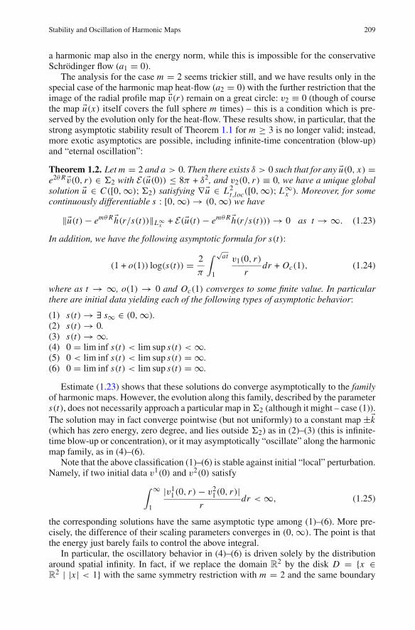
The analysis for the case m = 2 seems trickier still, and we have results only in thespecial case of the harmonic map heat-flow (a2 = 0) with the further restriction that theimage of the radial profile map �v(r) remain on a great circle: v2 ≡ 0 (though of coursethe map �u(x) itself covers the full sphere m times) – this is a condition which is pre-served by the evolution only for the heat-flow. These results show, in particular, that thestrong asymptotic stability result of Theorem 1.1 for m ≥ 3 is no longer valid; instead,more exotic asymptotics are possible, including infinite-time concentration (blow-up)and “eternal oscillation”:

Theorem 1.2. Let m = 2 and a > 0. Then there exists δ > 0 such that for any �u(0, x) =e2θR �v(0, r) ∈ �2 with E(�u(0)) ≤ 8π + δ2, and v2(0, r) ≡ 0, we have a unique globalsolution �u ∈ C([0,∞);�2) satisfying ∇�u ∈ L2

t,loc([0,∞); L∞x ). Moreover, for somecontinuously differentiable s : [0,∞)→ (0,∞) we have

‖�u(t)− emθR �h(r/s(t))‖L∞x + E(�u(t)− emθR �h(r/s(t)))→ 0 as t →∞. (1.23)

In addition, we have the following asymptotic formula for s(t):

(1 + o(1)) log(s(t)) = 2

π

∫ √at

1

v1(0, r)

rdr + Oc(1), (1.24)

where as t → ∞, o(1) → 0 and Oc(1) converges to some finite value. In particularthere are initial data yielding each of the following types of asymptotic behavior:

(1) s(t)→ ∃ s∞ ∈ (0,∞).(2) s(t)→ 0.(3) s(t)→∞.(4) 0 = lim inf s(t) < lim sup s(t) <∞.(5) 0 < lim inf s(t) < lim sup s(t) = ∞.(6) 0 = lim inf s(t) < lim sup s(t) = ∞.

Estimate (1.23) shows that these solutions do converge asymptotically to the familyof harmonic maps. However, the evolution along this family, described by the parameters(t), does not necessarily approach a particular map in�2 (although it might – case (1)).The solution may in fact converge pointwise (but not uniformly) to a constant map ±�k(which has zero energy, zero degree, and lies outside �2) as in (2)–(3) (this is infinite-time blow-up or concentration), or it may asymptotically “oscillate” along the harmonicmap family, as in (4)–(6).

Note that the above classification (1)–(6) is stable against initial “local” perturbation.Namely, if two initial data v1(0) and v2(0) satisfy

∫ ∞1

|v11(0, r)− v2

1(0, r)|r

dr <∞, (1.25)

the corresponding solutions have the same asymptotic type among (1)–(6). More pre-cisely, the difference of their scaling parameters converges in (0,∞). The point is thatthe energy just barely fails to control the above integral.

In particular, the oscillatory behavior in (4)–(6) is driven solely by the distributionaround spatial infinity. In fact, if we replace the domain R

2 by the disk D = {x ∈R

2 | |x | < 1} with the same symmetry restriction with m = 2 and the same boundary


conditions v(t, 0) = −�k and v(t, 1) = �k, then it is known [1] (see also [8]) that all thesolutions behave like (2), namely they concentrate at x = 0 as t → ∞, provided thatv3(0, r) has only one zero. The formula (1.24) suggests that we should always have (2)on D without the additional condition. Also, if we replace the domain R

2 by S2, then

we can rather easily show in the dissipative case a1 > 0 that the solution converges toone harmonic map for all m ∈ N, by the argument in this paper, or even those in theprevious papers. We state the result on S

2 in Appendix A with a sketch of the proof.We should mention that existence of eternal oscillation of the same type was first

shown in [18] for the semilinear heat equation of u(t, x) : [0,∞)× RN → R,

ut −�u = |u|pu, (1.26)

for very high dimensions and power2 (N ≥ 11 and p > 4/(N − 4 − 2√

N − 1)), byusing the comparison principle, but they did not obtain an asymptotic formula validfor all solutions, nor the asymptotic stability of the family of stationary solutions in asolution class containing the eternal oscillations.

There is another example in [21, Sect. 5] with less similarity to ours, but for theharmonic map heat flow, which shows existence of “eternal winding” around a compact1-parameter family of harmonic maps from S

2 to S2 × R

2 with some warped metric,where the analysis is reduced to an ODE on the target by the special choice of initial data.In this case, the weird behavior of the solutions is entirely due to the artificial choice ofthe metric on the target.

Compared with those results, we have the following advantages:

(1) The setting is very simple and physically natural.(2) The asymptotic formula is explicit in terms of the initial data, and valid for all

general solutions under the symmetry condition.

We want to emphasize also that our analysis works in the same way in the dissipative(a1 > 0) and the dispersive (a1 = 0) cases. We need a2 = 0 in Theorem 1.2 onlybecause the angular parameter α(t) gets beyond our control (hence we remove it by theconstraint), but the rest of our arguments could work in the general case.3

1.1. The main difficulty and the main idea. The standard approach for asymptotic sta-bility is to decompose the solution into a leading part with finite dimensional parametersvarying in time, and the rest decaying in time either by dissipation or by dispersion. Inour context, we want to decompose the solution in the form

�v(t) = �h[μ(t)] + v(t) (1.27)

such that the remainder v(t) decays, and the parameter μ(t) ∈ C converges as t →∞(at least for Theorem 1.1). In favorable cases (the higher m, in our context), we canchoose μ(t) such that all secular modes for v(t) are absorbed into the time evolution ofthe main part �h[μ(t)]. This means that the kernel of the linearized operator for v(t) isspanned by the parameter derivatives of �h[μ], and hence we can put that component of∂t �v(t) into ∂t �h[μ(t)]. This is good both for v(t) and μ(t), because

2 The power is bigger at least than the H5 scaling critical exponent.3 We will use the parameter convergence in the proof of Theorem 1.1 in the dispersive case a1 = 0 to

fix our linearized operator. However it is possible to treat the linearized operator even with non-convergentparameter and a1 = 0, if we assume one more regularity on the initial data. We do not pursue it here since thewild behavior of α(t) prevents us from using it.


(1) v(t)will be free from secular modes, and so we can expect it to decay by dissipationor dispersion, at least at the linearized level.

(2) The decomposition is preserved by the linearized equation. Hence μ(t) is affectedby v only superlinearly, i.e. at most in quadratic terms.

In particular, if we can get L2 decay of v in time, then μ(t) becomes integrable in time,and so converges as t →∞. This is indeed the case for m > 3.

However, the above naive argument does not take into account the space-time behav-ior of each component. The problem comes from the fact that the decomposition andthe decay estimate must be implemented in different function spaces, and they may beincompatible if the eigenfunctions decay too slowly at the spatial infinity.

In fact, the parameter derivative of �h[μ] is given by

d �h[μ] = hs1eαR[(hs

3, 0,−hs1)dμ1 + (0, 1, 0)dμ2], (1.28)

and hence the eigenfunctions are O(r−m) for r → ∞, i.e. slower for lower m. On theother hand, the spatial decay property in the function space for the time decay estimateis essentially determined by the invariance of our problem under the scaling

�v(t, x) �→ �v(λ2t, λx), (1.29)

which maps solutions into solutions, preserving the energy. If we want L2 decay in time(so that we can integrate quadratic terms in μ), then a function space with the rightscaling is given by

v/r ∈ L2t L∞x . (1.30)

To preserve such norms in x under the orthogonal projection, the eigenfunction mustbe in the dual space, for which m > 3 is necessary. Indeed, this is the essential reasonfor the restriction m ≥ 4 in the previous works [10–12]. We emphasize that the abovedifficulty is common for the dissipative and dispersive cases, since they share the samescaling property. That is, the dissipation does not help with this issue, even though itgives us more flexibility in the form of decay estimates.

The main novelty of the present approach is the non-orthogonal decomposition

L2x = (hs

1)⊕ (ϕs)⊥, (1.31)

where ϕs(r) is smooth and supported away from r = 0 and from r = ∞, so thatthe (non-orthogonal) projection may preserve the decay estimates. This is good for theremainder v, but not for the parameter μ —the decomposition is no longer preservedby the linearized evolution, since they have no particular relation. This implies that weget a new error term in μ(t) which is linear in v(t) (see Sect. 6). This contribution ishandled by including it in a sort of “normal form” for the dynamics of the parametersμ(t), explained in Sect. 7. In particular, it is this new term which drives the non-trivialdynamics for the m = 2 heat-flow given in Theorem 1.2.

For the purely dispersive (Schrödinger map) case, one tool we use should be ofsome independent interest: the 2D radial “double-endpoint Strichartz estimate” forSchrödinger operators with sufficiently “repulsive” potentials (in the absence of a poten-tial, the estimate is false). The proof is given in Sect. 10.2.


1.2. Organization of the paper. In Sect. 2, we use the “generalized Hasimoto transform”to derive the main equation used to obtain time-decay estimates of the remainder term.Section 3 gives the details of the solution decomposition described above, and addressesthe inversion of the Hasimoto transform. The estimates for going back and forth betweenthe different coordinate systems (the “Hasimoto” one of Sect. 2 and the decompositionof Sect. 3) are given in Sect. 4. Section 5 is devoted to establishing the time-decay (dis-persive if a1 = 0, diffusive if a1 > 0) of the remainder term, using energy-, Strichartz-,and scattering-type estimates. The dynamics of the parameters μ(t) are derived andestimated in Sect. 6. The leading term in the equation for μ is not integrable in time,and so Sect. 7 gives an integration by parts in time to identify (and estimate) a kind of“normal form” correction to μ(t), whose time derivative is integrable. At this stage, theproof of Theorem 1.1 for m > 3 is complete. A more subtle estimate of an error termfor m = 3 is done in Sect. 8, completing the proof in that case. Finally, in Sect. 9, thenormal form correction is analyzed in the case m = 2, a2 = 0, v2 = 0, in order to proveTheorem 1.2. Proofs of certain linear estimates (including the double-endpoint Stri-chartz) are relegated to Sect. 10. Appendix A states the analogous theorems for domainS

2 and sketches the proofs.At the end of each of the main sections, we will put a proposition summarizing the

main contents of that section.

1.3. Some further notation. We distinguish inner products in R3 and C by

�a · �b =3∑

k=1

akbk, a ◦ b = Re a Re b + Im a Im b. (1.32)

Both will be used for C3 vectors too. The L2

x inner-product is denoted

( f | g) =∫

R2f (x)g(x)dx, (1.33)

while ( f, g) just denotes a pair of functions. For any radial function f (r) and any param-eter s > 0, we denote rescaled functions by

f s(r) := f (r/s), f �s(r) := f (r/s)s−2. (1.34)

We denote the Fourier transform on R2 by F , and, for radial functions, the Fourier-Bessel

transform of order m by Fm :

(F f )(ξ) = 1

2π

∫R2

f (x)e−i x ·ξdx, (Fm) f (ρ) =∫ ∞

0Jm(rρ) f (r)rdr, (1.35)

where Jm is the Bessel function of order m. For m ∈ Z we have

Jm(r) = 1

2π

∫ π

−πeimθ−ir sin θdθ, F[ f (r)eimθ ] = im(Fm f )eimθ . (1.36)

We denote the Laplacian �x on the subspace spanned by d-dimensional spherical har-monics of order m by

�(m)d := ∂2

r + (d − 1)r−1∂r − m(m + d − 2)r−2. (1.37)

Finally, the space L pq is the dyadic version of L p(rdr) defined by the norm

‖ f ‖L pq=

∥∥∥‖ f (r){2 j < r < 2 j+1}‖L p(rdr)

∥∥∥�

qj (Z)

. (1.38)


2. Generalized Hasimoto Transform

In this section, we recall from the previous papers [9–11] the equation for the remainderpart, which is written in terms of a derivative vanishing exactly on the harmonic maps,and so independent of the decomposition. The equation was originally derived in [6] inthe case of small energy solutions (hence with no harmonic map component), and calledthere the generalized Hasimoto transform.

Under the m-equivariance assumption (1.13), the Landau-Lifshitz equation (1.6) isequivalent to the following reduced equation for �v(r, t):

�vt = P �va[∂2

r +∂r

r+

m2

r2 R2]�v. (2.1)

Define the operator ∂�v on vector-valued functions by

∂�v := ∂r − m

rJ �vR. (2.2)

Since for any vector �b, J �vR�b = �k(�v · �b) − (�k · �v)�b, we have J �vR = −v3 on the tan-gent space T�vS2 = �v⊥. For future use, we denote the corresponding operator on scalarfunctions by

L �v := ∂r +mv3

r. (2.3)

Then Eq. (2.1) can be factored as

�vt = −P �va D∗�v∂�v �v, (2.4)

where

D := P �v∂P �v (2.5)

will always denote a covariant derivative (which acts on T�vS2-valued functions), and ∗denotes the adjoint in L2(R2). Denote the right-most factor in (2.4) by

�w := ∂�v �v = �vr − m

rP �v �k. (2.6)

Then (2.4) becomes �vt = −P �va D∗�v �w, and applying D�v to both sides yields

Dt �w = −P �va D�vD∗�v �w. (2.7)

Now we rewrite the equation for �w by choosing an appropriate orthonormal frame fieldon T�vS2, realized in C

3. Let e = e(t, r) satisfy

Re e ∈ �v⊥, |Re e| = 1, Im e = J �v Re e. (2.8)

Let S, T be real scalar, and let q, ν be complex scalar, defined by

�w = q ◦ e, P �v �k = ν ◦ e, Dt e = −i Se, Dr e = −iT e. (2.9)

Then we have the general curvature relation

[Dr , Dt ]e = i(Tt − Sr )e = i det(�v �vr �vt

)e. (2.10)


Using Eq. (2.4) for �v, we get

Tt − Sr = ( �w +m

rP �v �k) · P �via D∗�v �w. (2.11)

Now we fix e by imposing

Dr e = 0, e(r = ∞) = (1, i, 0). (2.12)

(The unique existence of such e will be guaranteed by Lemma 4.1.) Then (2.11) yields

− Sr = (q +m

rν) ◦ (iaL∗�vq). (2.13)

A key observation is that in the Schrödinger (non-dissipative) case a = i , we can pullout the derivative on q: Sr = (∂r + 2

r )(12 |q|2 + m

r ν◦ q), and so

S = −Q +∫ ∞

r2Q

dr

r, Q := 1

2|q|2 +

m

rν ◦ q = 1

2| �w|2 +

mw3

r. (2.14)

The evolution equation (2.7) for w yields our equation for q:

(∂t + i S)q = −aL �vL∗�vq, S =∫ ∞

r(q +

m

rν) ◦ (iaL∗�vq)dr. (2.15)

This is the basic equation used to establish diffusive (a1 > 0) or dispersive (a1 = 0)decay estimates. The operator acting on q can be expanded as

L �vL∗�v = ∂∗r ∂r +(m − 1)2

r2 +2m(1− v3)

r2 +m

rw3. (2.16)

Following is a summary of this section:

Proposition 2.1. Let m ∈ N and �u(t, x) = emθR �v(t, r) be a (local) solution of theLandau-Lifshitz equation (1.1), and let e(t, r) be a complex orthonormal frame field onT�vS2 satisfying

Dr e = 0, e(r = ∞) = (1, i, 0), (2.17)

where D denotes the covariant derivative (2.5). Define �w, q and ν by

�w = �vr − m

rP �v �k, q = �w · e, ν = P �v �k · e. (2.18)

Then they solve equations

(∂t + i S)q = −aLvL∗vq, S =∫ ∞

r(q +

m

rν) ◦ (iaL∗vq)dr, (2.19)

where Lv = ∂r +mv3/r and L∗v is its adjoint. If a = i , the equation of S can be rewrittenas

S = −Q +∫ ∞

r2Q

dr

r, Q = 1

2|q|2 +

m

rν ◦ q. (2.20)

We will use the above equations to derive decay estimates on the remainder �v− �h[μ]via q. The following two sections are devoted to the correspondence between q andthe remainder (including the existence of e), and then in Sect. 5 we derive the decayestimates.


3. Decomposition and Orthogonality

In this section, we investigate the interplay between the decay estimates and the orthog-onality condition for the decomposition into the harmonic map and the remainder, illu-minating the difference between the higher and the lower degrees.

We introduce coordinates for the decomposition of the original map

�v = �h[μ] + v, (3.1)

or more precisely for the remainder v, and a localized orthogonality condition whichdetermines the decomposition. The choice of coordinates is the same as in the previousworks [9,10,12], while the decomposition itself is different.

For each harmonic map profile �h[μ], μ = m log s + iα, we introduce an orthonormalframe field

f = f[μ] := eαR(−�hs × �j + i �j) (3.2)

on the tangent space T�h[μ]S2, such that the parameter derivative of �h[μ] is given by

d �h[μ] = hs1dμ ◦ f . (3.3)

We express the difference from the harmonic map in this frame by

z := v · f . (3.4)

In other words P �h[μ] �v = z ◦ f , or v = z ◦ f + γ �h[μ], where we denote

γ :=√

1− |z|2 − 1 = −O(|z|2). (3.5)

As explained in the Introduction, the orthogonality condition in the previous works

(z | hs1) = 0 (3.6)

would not work for m ≤ 3 due to the slow decay of hs1 for r → ∞. Hence instead we

determine the parameter μ by imposing localized orthogonality

(z | ϕs) = 0, ϕs = ϕ(r/s), (3.7)

with some smooth localized function ϕ(r) ∈ C∞0 ((0,∞);R), satisfying (h1 | ϕ) = 1.The fact that emθR �h[μ] solves (1.11) means that

∂�h �h = 0, (3.8)

and so we have

�w = ∂�v �v = vr +m

r(hs

3v + v3�v) = Ls v +m

rv3�v. (3.9)

Hence

Ls z = Ls v · f + v · fr = �w · f − m

rv3z +

m

rhs

1γ. (3.10)


In order to estimate z by �w (or equivalently q), we introduce a right inverse of theoperator Ls = ∂r + m

r hs3, defined by

Rsϕg := 2πhs

1(r)∫ ∞

0

∫ r

r ′hs

1(r′′)−1g(r ′′)dr ′′ϕ �s(r ′)hs

1(r′)r ′dr ′. (3.11)

Then we have

Ls Rsϕg = g, Rs

ϕLs g = g − hs1(g | ϕ �s), (3.12)

hence Rsϕ = (Ls)−1 on (ϕs)⊥. Moreover we have the following uniform bounds

Lemma 3.1. For all p ∈ [1,∞] and |θ | < m, we have

‖Rsϕg‖rθ L∞p � ‖ϕ‖r−θ L1

p′‖g‖rθ+1 L1

p, (3.13)

where the L pq norm is defined in (1.38). Moreover, the condition on ϕ is optimal in

the following sense: if ϕ ≥ 0, then ϕ ∈ r−1L1p′ is necessary for Rs

ϕ to be bounded

r θ−1L∞p → D′(0,∞).We give a proof in Sect. 10. Note that the above bounds are scaling invariant: denoting

Ds f := f (r/s), we have

Rsϕ = s Ds R1

ϕD−1s , Ls = s−1 Ds L1 D−1

s . (3.14)

We can combine the estimates of the lemma with the embedding

r θ1 L p1q1 ⊂ r θ2 L p2

q2 ⇐⇒2

p1− θ1 = 2

p2− θ2, p1 ≥ p2, q1 ≤ q2. (3.15)

The above lemma is used as follows. First note that the orthogonality (ϕs | z) = 0implies that z = Rs

ϕLs z because of (3.12). For the energy norm, we choose θ = 0 andp = 2 in Lemma 3.1. Then

‖z/r‖L2x

� ‖z‖L∞2 � ‖ϕ‖L12‖Ls z‖r L1

2� ‖Ls z‖L2

x. (3.16)

Since |Ls − ∂r | � 1/r , we further obtain

Rsϕ : r θ L2 → r θ X, (|θ | < m), (3.17)

where the space X is defined by the norm

‖z‖X := ‖z/r‖L2x

+ ‖zr‖L2x. (3.18)

The Sobolev embedding X ⊂ L∞ is trivial by Schwarz:

‖z‖2L∞x ≤ ‖z/r‖L2x‖zr‖L2

x. (3.19)

Hence we get by using (3.10),

‖z‖X � ‖Ls z‖L2 � ‖q‖L2 + ‖z‖L∞‖z‖X . (3.20)


For L2t estimates of z, we use Lemma 3.1 with θ = 1 and p = ∞. Then we have

‖z/r‖L∞p � ‖ϕ‖r−1 L11‖Ls z‖r2 L1

p� ‖Ls z‖L∞p , (3.21)

for any p ∈ [1,∞], and so by using (3.10),

‖z/r‖L2t L∞p � ‖q‖L2

t L∞p + ‖z‖L∞t,x ‖z‖L2t L∞p . (3.22)

If we were to use h1 instead of ϕ, then we would need m > 3 for the Strichartz-typebound (3.22), and m > 2 for the energy bound (3.16), by the last statement of the lemma.

As a summary of this section, we have

Proposition 3.2. Let m ≥ 2, �v(r) ∈ �m and, for some μ = m log s + iα ∈ C,

�v = �h[μ] + v, z = v ◦ f, (3.23)

where f is the orthonormal frame on T�h[μ]S2 defined in (3.2). Suppose that

(z|ϕs) = 0, ϕs := ϕ(r/s) (3.24)

for a fixed ϕ ∈ C0(0,∞) satisfying (h1|ϕ) = 1. Then we have the estimates

‖z‖X := ‖z/r‖L2x

+ ‖zr‖L2x

� ‖q‖L2x

+ ‖z‖L∞x ‖z‖X ,

‖z/r‖L∞p � ‖q‖L∞x + ‖z‖L∞x ‖z‖L∞p (1 ≤ p ≤ ∞), (3.25)

‖z‖L∞x � ‖z‖X ,

where q = �w · e is the same as in Proposition 2.1.

In the next section, we see that such an orthogonal decomposition uniquely exists for�v ∈ �m with energy close to the ground one, with small norms for q and z, so that wecan dispose of the quadratic terms in the above estimates.

4. Coordinate Change

Before beginning the estimates for the evolution, we establish in this section the bi-Lips-chitz correspondence between the different coordinate systems: �v and (μ, q), includingunique existence of the decomposition. It is valid for any map in our class �m withenergy close to the ground states.

For that purpose, we need to translate between the different frames e and f . At eachpoint (t, r), we define M = f ⊗ e ∈ GLR(C), a real-linear map C→ C, by

Mz := f · (e ◦ z). (4.1)

Its transpose tM = e ⊗ f , defined by tMz = e · (f ◦ z), is the adjoint in the sense that(Mz) ◦w = z ◦ (tMw). For any b, c,d ∈ C

3 we have

b · (c ◦ d) = (Re b · c) ◦ d + (Im b · c) ◦ d. (4.2)

Since f(∞) = e−iαe(∞), and f ⊥ �h[μ], we have

M(∞) = e−iα, Mr = f ⊗ er + fr ⊗ e = −f ⊗ v(e · �vr )− m

rhs

1v ⊗ e. (4.3)


Then e can be recovered from M by

e = P�h[μ]e + (�h[μ] · e)�h[μ] = tMf − (1 + γ )−1(tMz)�h[μ], (4.4)

provided that |γ | < 1. We further introduce some spaces with (pseudo-)norms:

Em(�v) = E(emθR �v(r)), |μ|C = min(|Reμ|, 1) + dist (Imμ, 2πZ),

‖z‖X = ‖z/r‖L2x

+ ‖zr‖L2x, ‖M‖Y = ‖Mr‖L1(dr) + ‖M‖L∞r ,

�m(δ) = {�v(r) : [0,∞] → S2 | �v(0) = −�k, �v(∞) = �k, Em(�v) ≤ 4mπ + δ2},

L2(δ) = {q(r) : [0,∞)→ C | ‖q‖L2x≤ √2δ}, C = C/2π iZ.

(4.5)

The metric on C is defined such that

‖�h[μ1] − �h[μ2]‖X ∼ ‖�h[μ1] − �h[μ2]‖L∞ ∼ |μ1 − μ2|C . (4.6)

The following lemma is the goal of this section.

Lemma 4.1. Let m ∈ N and ϕ ∈ C10(0,∞) satisfy (ϕ | h1) = 1. Then there exists δ > 0

such that the system of equations

�v = �h[μ] + v, z = �v · f[μ], (z | ϕs) = 0, γ =√

1− |z|2 − 1,

q = e ◦ (�vr − m

rP �v �k), Dr e = 0, e(∞) = (1, i, 0),

(4.7)

defines a bijection from �v ∈ �m(δ) to (μ, q) ∈ C × L2(δ), which is unique under thecondition ‖z‖L∞x � δ. v, z and e are also uniquely determined. Moreover, if (�v j , . . . , e j )

with j = 1, 2 are such tuples given in this way, then we have

‖v1 − v2‖X + ‖z1 − z2‖X + ‖e1 − e2‖L∞ + ‖M1 −M2‖Y

� ‖�v1 − �v2‖X ∼ |μ1 − μ2|C + ‖q1 − q2‖L2 , (4.8)

where M j := f j ⊗ e j .

In particular, we have pointwise smallness,

‖v‖L∞x ∼ ‖z‖L∞x � δ � 1, (4.9)

so that we can neglect higher order terms in z or v.

Proof. We always assume (3.9), (3.4) and (3.5), which define the maps

�v �→ �w = q ◦ e, (�v, μ) �→ v ↔ z �→ γ, (v, μ) �→ �v, (4.10)

with the Lipschitz continuity

‖ �w1 − �w2‖L2 � ‖�v1 − �v2‖X , ‖γ 1 − γ 2‖X � ‖z1 − z2‖X ∼ ‖v1 − v2‖X ,∣∣∣‖�v1 − �v2‖X − ‖v1 − v2‖X

∣∣∣ � |μ1 − μ2|C . (4.11)


The energy can be written as

2Em(�v) = ‖�vr‖2L2x

+∥∥∥m

rR�v

∥∥∥2

L2x

= ‖�vr‖2L2x

+∥∥∥m

rP �v �k

∥∥∥2

L2x

= ‖ �w‖2L2x

+ 2m(�vr | P �v �k/r) = ‖ �w‖2L2x

+ 4π [v3(∞)− v3(0)]. (4.12)

Since ‖P �k �v‖X � Em(�v)1/2, X ⊂ L∞x and |�v| = 1, the boundary conditions v3(0) = −1and v3(∞) = 1 make sense in the energy norm.

Next we consider a point orthogonality. Let �v ∈ �m(δ). Since v3(0) < 0 < v3(∞)and v3(r) is continuous, we have �v(s0) = eiα0 R �h(1) for some μ0 = m log s0 + iα0, sothat �v = �h[μ0] + v is a decomposition satisfying (z | ϕs0) = 0 if ϕ(r) = δ(r − 1). Inthis case �v is recovered from ( �w,μ0) by solving the ODE:

Ls z = �w · f[μ0] − m

rv3z +

m

rhs0

1 γ, z(s0) = 0, (4.13)

or the equivalent integral equation

z = Rs0δ(r−1)

[�w · f[μ0] − m

rv3z +

m

rhs0

1 γ]. (4.14)

The uniform bound on Rsδ(r−1) can be localized onto any interval I s0, because z is the

solution of the above initial value problem. Hence we get, in the same way as in (3.16),

‖z‖r L2x∩L∞x (I ) � ‖q‖L2

x (I )+ ‖z‖L∞x (I )‖z‖r L2

x (I ). (4.15)

Since z(s0) = 0 and ‖q‖L2x≤ δ � 1, we get by continuity in r for I → (0,∞),‖z‖X∩L∞x � ‖q‖L2

x� δ. (4.16)

Thus every �v ∈ �m(δ) is close at least to some �h[μ0], and we have �v1 − �v2 ∈ X by(4.11). �m(δ) is a complete metric space with this distance.

Now we take any ϕ ∈ C10(0,∞) satisfying (ϕ | h1) = 1, and look for μ around μ0

solving the orthogonality

F(μ) := (�v · f[μ] | ϕ �s) = (v · f[μ] | ϕ �s) = (z | ϕ �s) = 0. (4.17)

Its derivative in μ is given by

d F = −(�v · hs1�h[μ] | ϕ �s)dμ− i(�v · hs

3f[μ] | ϕ �s)dα − (�v · f[μ] | (r∂r + 2)ϕ �s)ds

s= −dμ− (v · �h[μ] | hs

1ϕ�s)dμ− (v · f[μ] | (r∂r + 2)ϕ �sds/s + ihs

3ϕ�sdα)

= −dμ + O(δ|dμ|). (4.18)

In particular we have

|F(μ0)| � δ,∂F

∂μ(μ0) = −I + O(δ). (4.19)

In addition, both F(μ) and ∂μF are Lipschitz in �v. Therefore by the implicit mappingtheorem, if δ > 0 is small enough, there exists a unique μ ∈ C for each v such thatF(μ) = 0 and |μ− μ0| � δ, and �v �→ μ is Lipschitz. Then

‖z‖L∞x � ‖�v − �h[μ0]‖L∞x + |μ0 − μ| � δ � 1, (4.20)


and so by the same argument as for (4.16), we get ‖z‖X � δ, and in addition,

‖z1 − z2‖X � |μ1 − μ2|C + ‖ �w1 − �w2‖L2 . (4.21)

If we have two such μ = μ1, μ2 with ‖z j‖L∞ � δ, then

|μ1−μ2|C ∼ ‖�h[μ1]−�h[μ2]‖L∞x � ‖�v−�h[μ1]‖L∞x +‖�v − �h[μ2]‖L∞x � δ, (4.22)

and so the implicit mapping theorem implies that μ1 = μ2. Thus we get a bijection�v �→ (μ, �w) with the Lipschitz continuity

‖�v1 − �v2‖X ∼ |μ1 − μ2|C + ‖ �w1 − �w2‖L2x. (4.23)

For the frame field e, we consider the matrix M = f⊗e, together with the equivalentset of Eqs. (4.3) and (4.4). Integrating (4.3) from r = ∞, we get

‖M− eiα‖Y � ‖v/r‖L2x‖�vr‖L2

x+ ‖v/r‖L2

x‖hs

1/r‖L2x

� δ,

‖M1 −M2‖Y � |μ1 − μ2|C + δ‖�v1 − �v2‖X + δ‖e1 − e2‖L∞ + ‖v1 − v2‖X ,(4.24)

while (4.4) provides

‖e1 − e2‖L∞x � ‖M1 −M2‖L∞x + |μ1 − μ2|C + ‖z1 − z2‖L∞x . (4.25)

Hence for fixed �v ∈ �m(δ) (and μ), we can get (M, e) ∈ Y × L∞ by the contractionmapping principle for the system of (4.3) and (4.4). Moreover we get

‖M1 −M2‖Y + ‖e1 − e2‖L∞x � ‖�v1 − �v2‖X . (4.26)

If (μ, q) ∈ C × L2(δ) is given, we consider the system of Eqs. (4.3), (4.4) and

z = Rsϕ

[Mq − m

rv3z +

m

rhs

1γ], (4.27)

which is equivalent to the q equation in (4.7) under the orthogonality (z | ϕ �s) = 0. Thelast equation provides, through the uniform bound on Rs

ϕ ,

‖z1−z2‖X � |μ1 − μ2|C + ‖q1 − q2‖L2x+δ‖M1 −M2‖Y + δ‖z1 − z2‖X . (4.28)

Combining this with (4.24) and (4.25), we get (z,M, e) for any fixed (μ, q) by thecontraction mapping, and moreover they satisfy

‖z1 − z2‖X + ‖M1 −M2‖Y + ‖e1 − e2‖L∞ � |μ1 − μ2|C + ‖q1 − q2‖L2x. (4.29)

"#So far we have derived estimates at each fixed t , for the energy norms in the above

lemma, and for the dispersive norms in Proposition 3.2. Now we turn to the main partof this paper, the analysis of the global dynamics.


5. Decay Estimates for the Remainder

In this section, we derive dissipative or dispersive space-time estimates of the remainderv in terms of z, from Eq. (2.15) for q. First by the smallness of z, we obtain from (3.20)and (3.22),

‖z(t)‖X � ‖q(t)‖L2 � δ, ‖z/r‖L∞p � ‖q‖L∞p , (5.1)

for all p ∈ [1,∞]. Next we estimate the factor S, by using

‖r∫ ∞

rf gdr‖L∞1 �

∑j∈Z

∑k≥ j

2 j−k‖ f g‖L1(r∼2k ) ∼ ‖ f g‖L1 ≤ ‖ f ‖L2‖g‖L2 . (5.2)

Then from the expression in (2.15) for S, we have

‖S(t)‖L21

� ‖S(t)‖r−1 L∞1 � (‖q‖L2x

+ ‖z‖r L2x

+ 1)‖L∗�vq‖L2x

� ‖L∗�vq‖L2x. (5.3)

In the dispersive case a1 = 0, we avoid the derivative by using expression (2.14)

‖S(t)‖L21

� ‖S(t)‖r−1 L∞1 � (‖q‖L2x

+ ‖z‖r L2x

+ 1)‖q‖L∞2 � ‖q‖L∞2 (a1 = 0).

(5.4)

For the time decay estimates, we treat the dissipative and the dispersive cases separately.

5.1. Dissipative L2t estimate. Here we assume a1 > 0. By Eq. (2.15) of q, we have

∂t‖q‖2L2 = −2a1‖L∗�vq‖2L2 , (5.5)

hence

‖q‖L∞t L2x

+ ‖L∗�vq‖L2t L2

x� ‖q(0)‖L2

x∼ δ. (5.6)

Since Rs∗ϕ Ls∗ = I and Rs∗

ϕ : L2 → r L2 by Lemma 3.1 and duality, we have

‖q‖r L2x

� ‖Ls∗q‖L2x

� ‖L∗�vq‖L2x

+ ‖v‖L∞‖q‖r L2x. (5.7)

Since the last term can be absorbed by (4.9) smallness of v, we get

‖q‖X � ‖q/r‖L2x

+ ‖Ls∗q‖L2x

� ‖L∗�vq‖L2x. (5.8)

So by using the bound (3.17) on Rsϕ , we obtain

‖z‖r L2t X � ‖q‖L2

t X � ‖L∗�vq‖L2t,x

� ‖q(0)‖L2x∼ δ, (5.9)

and also from (5.3),

‖S‖L2t L2

x� δ. (5.10)


5.2. Dissipative decay. Next we show the convergence q → 0 as t →∞, by comparingit with the free evolution. For T > 0, let

qT := q − e(t−T )a�(m−1)2 q(T ). (5.11)

Then we have

qTt − a�(m−1)

2 qT = (i S − aV )q, qT (T ) = 0, (5.12)

where the potential V (t, x) is given by

V = 2m(1− v3)

r2 +m

rw3. (5.13)

Multiplying the equation with qT , we get the energy identity

1

2‖qT ‖2L2

x+

∫ t

Ta1(‖qT

r ‖2L2x

+ ‖m − 1

rqT ‖2L2

x)dt

= Re∫ t

T(−aV q + i Sq | qT )dt, (5.14)

and hence by Schwarz, and using estimate (5.3) to put S ∈ L2t L2

x ,

‖qT ‖L∞t>T L2x∩L2

t>T X � ‖q/r‖L2t>T L2

x+ ‖Sq‖L2

t>T L1x

+ ‖q‖2L4

t>T L4x

� ‖q/r‖L2t>T L2

x+ ‖q‖L∞t L2

x‖q‖L2

t>T X → 0 (T →∞). (5.15)

Hence ‖q(t)‖L2x

can not converge to a positive number, since e(t−T )a�(m−1)2 q(T ) → 0

as t →∞ for all T > 0. Thus we obtain

‖z(t)‖X � ‖q(t)‖L2x→ 0 (t →∞). (5.16)

5.3. Dispersive L2t estimate. Next we consider the case a1 = 0 (and a2 �= 0). We set

(with no loss of generality) a = i . Since the energy identity provides only L2x bound

on q, we have to work with the Strichartz estimate in a perturbative way. DenotingHs := Ls Ls∗, the equation of q is given by

qt + i Hs(0)q = N1 + N2, (5.17)

where

N1 := −2amhs(0)

3 − hs(t)3

r2 q, N2 := i Sq − 2amv3

r2 q − amw3

rq, (5.18)

and S is given by (2.14). We have

|N1| � |h3(s(t)/s(0))||q|/r2, (5.19)

and so

‖N1‖L2t L1

2� ‖h3(s(t)/s(0))‖L∞t ‖q‖L2

t L∞2. (5.20)


Using (5.4), we have

‖Sq‖L1t L2

x≤ ‖S‖L2

t L2x‖q‖L2

t L∞x � ‖q‖2L2

t L∞2. (5.21)

The other terms in N2 are bounded in L1t L2

x by

‖q‖2L2

t L∞2+ ‖z/r‖L2

t L∞2‖q‖L2

t L∞2� ‖q‖2

L2t L∞2

. (5.22)

Now we need the endpoint Strichartz estimate for Hs with fixed scaling s:

Lemma 5.1. Let Hs = Ls Ls∗ = −�(m−1)2 + 2mr−2(1− hs

3) and m > 1. Then we have

‖e−i Hs tϕ‖L∞t L2x∩L2

t L∞2� ‖ϕ‖L2

x

‖∫ t

−∞e−i Hs (t−t ′) f (t ′)dt ′‖L∞t L2

x∩L2t L∞2

� ‖ f ‖L1t L2

x +L2t L1

2,

(5.23)

uniformly for any fixed s > 0.

This lemma will be proved in Sect. 10.2. Hence if | log(s(t)/s(0))| � 1 for all t ,then we have

‖q‖L∞t L2x∩L2

t L∞2� ‖q(0)‖L2 ∼ δ, (5.24)

and also from (5.4)

‖S‖L2t L2

x� δ. (5.25)

5.4. Dispersive decay. Next we prove the following asymptotics of scattering type forq and z:

e−i t�(m−1)2 q(t)→ ∃q+ in L2

x , z → 0 in L∞x (t →∞). (5.26)

For the scattering of q, we further expand the equation

qt − i�(m−1)2 q = N0 + N2, (5.27)

where N2 is as in (5.18), and

N0 := −2am1− hs

3

r2 q. (5.28)

Then the global Strichartz bound implies that

‖N0‖L2t L1

2(T,∞)→ 0, ‖N2‖L1t L2

x (T,∞)→ 0 (5.29)

as T →∞. By Strichartz (for �(m−1)2 ) once again, we get the scattering of q.

For the vanishing of z, we use the inversion formula

z = Rsϕg, g =Mq + r−1m(hs

1γ − v3z). (5.30)


Since Rsϕ is bounded L2

x → L∞, the latter two terms contribute at most with ‖z‖L∞x ‖z/r‖L2

x� ‖z‖L∞x , hence we may drop them. Also we may replace q by its asymptotic free

solution q∞ := eit�(m−1)2 q+. Moreover we may approximate q+ by nicer functions.

Hence we assume that q := Fm−1q+ ∈ C∞0 (0,∞). Then we may further replace thefree solution with the stationary phase part:

q∞(t, r) = Cmt−1eir2/(4t)∫ ∞

0Jm−1(rρ/(2t))eiρ2/(4t)q+(ρ)ρdρ

= Cmt−1eir2/(4t)q(r/(2t)) + R, (5.31)

where the error is bounded by Plancherel

‖R‖L2x∼ ‖(1− eir2/(4t))q+‖L2

x� t−1‖r2q+‖L2

x→ 0. (5.32)

Now that spatially local vanishing is clear (eg. it follows from ‖RsϕMq(t)‖r L∞ �

‖q∞(t)‖L∞ → 0), we may extract the leading term of Rsϕ for large x . We assume

that s(t) ∈ L∞t and suppϕs ⊂ (0, b) for a fixed b ∈ (0,∞). Then for r > b we have

(Rsϕg)(r) = o(1) +

∫ r

b

hs1(r)

hs1(r′′)

g(r ′′)dr ′′

= o(1) +∫ r

b(r ′/r)m g(r ′)dr ′ as r →∞. (5.33)

Thus we are reduced to showing that

Gχ :=∫ r

b(ρ/r)mM(t, ρ)t−1eiρ2/(4t)χ(ρ/t)dρ → 0 in L∞r (5.34)

for any χ ∈ C∞0 (0,∞). By partial integration on (ρ/t)eiρ2/(4t), we have

rm Gχ = (i/2)[ρm−1M(ρ)eiρ2/(4t)χ(ρ/t)]rb−

∫ r

b

[(m − 1)M(ρ)χ(ρ/t)/ρ + M(ρ)χ ′(ρ/t)/t

+ Mr (ρ)χ(ρ/t)] ρm−1eiρ2/(4t)dρ. (5.35)

The right-hand side is bounded by rm/t , using |χ(ρ/t)| � ρ/t for the first, second andfourth terms, |χ ′(ρ/t)| � 1 for the third, and Mr ∈ L∞t L1(dr) for the fourth term.Thus we obtain ‖z(t)‖L∞x → 0.

Thus we have obtained the following a priori estimates in this section

Proposition 5.2. Let m ≥ 2 and �u(t, x) = emθRv(t, r) be a solution of (1.1) on 0 <t < T with �u(0) ∈ �m and E(�u(0)) ≤ 4mπ + δ2 for some small δ > 0. Let q, z, S be asin Proposition 2.1, and let μ(t) be given by Lemma 4.1.

(I) If a1 > 0, then we have

‖z‖L∞t (0,T ;X)∩L2t (0,T ;r X) � ‖q‖L∞t (0,T ;L2

x )∩L2t (0,T ;X) � ‖q(0)‖L2

x∼ δ. (5.36)

Moreover, if T = ∞ then

‖z(t)‖X � ‖q(t)‖L2x→ 0 (t →∞). (5.37)


(II) If a1 = 0 and s(t) = s(0) + O(δ), then we have

‖z‖L∞t (0,T ;X)∩L2t (0,T ;r L∞2 )

�‖q‖L∞t (0,T ;L2x )∩L2

t (0,T ;L∞2 )�‖q(0)‖L2x∼ δ.

(5.38)

Moreover, if T = ∞ and s(t) converges as t →∞, then

‖z(t)‖L∞x → 0, ‖q(t)− e−i t�(m−1)2 q+‖L2

x→ 0, (t →∞) (5.39)

for some radial q+ ∈ L2x .�(m−1)

2 is the (m− 1)-equivariant Laplacian, see (1.37).

Note that the decay of z is transferred to the remainder v by Lemma 4.1. By usingthe above arguments and Lemma 4.1, it is easy to see that the solution is global unlesss(t)→ 0 in finite time (for a detailed proof, see [11, Sect. 3]). The remaining sectionsare therefore devoted to the analysis of the parameter dynamics, which is the most novelpart of this paper.

6. Parameter Evolution

It remains to control the asymptotic behavior of the parameter μ(t) of the harmonicmap part of the solution. Its evolution is determined by differentiating the localizedorthogonality condition

0 = ∂t (z | ϕs) = (vt · f | ϕs) + (v · ft | ϕs) + (z | ∂tϕs), (6.1)

and each term on the right is expanded by using

vt = �vt − �h[μ]t = −(aL∗�vq) ◦ e − hs1μ ◦ f,

ft = −ihs3αf − hs

1μh[μ], ∂tϕs = − s

sr∂rϕ

s .(6.2)

Plugging this into the above and then dividing it by s2, we get

μ = −(MaL∗�vq | ϕ �s)− (hs1μγ | ϕ �s)− (z | (

μ1

mr∂r − iμ2hs

3)ϕ�s). (6.3)

The last two terms are bounded by

|μ|‖z‖L∞(‖ϕ‖L1 + ‖r∂rϕ‖L1), (6.4)

and so absorbed by the left-hand side since ‖z‖L∞ � δ � 1.Since |ν| = |Pv �k| � hs

1 + |v| and hence

|�vr | � |q| + |z|/r + hs1/r, (6.5)

we get from (4.3),

|Mr | � |qz| + |z|2/r + |zhs1|/r. (6.6)

The leading (first in the r.h.s) term in (6.3) can be estimated, using [Ma, L∗�v] =Mr a,as follows:

|(MaL∗�vq | ϕ �s)| � s−1(‖Mr‖L2x

+ ‖M‖L∞x )‖q‖r L2x

� s−1(‖q‖L2x

+ ‖z/r‖L2x

+ 1)‖q‖r L2x. (6.7)


Hence using that ‖z‖L∞x � ‖z‖X � ‖q‖L2 � δ � 1, we get

‖sμ‖L2t

� ‖q/r‖L2t,x

� ‖q‖L2t L∞2

. (6.8)

Then the last two terms of (6.3) are bounded in L1t by

‖sμ‖L2t‖z/r‖L2

t L∞x ‖(r |ϕ| + r2|ϕr |) �s‖L1x

� ‖q‖2L2

t L∞2, (6.9)

where we used (5.1). Thus we have obtained

Proposition 6.1. Let �v, q, μ, ϕ and M as in Proposition 5.2 and Lemma 4.1. Then μ(t)satisfies

μ = −(MaL∗�vq | ϕ �s) + error, (6.10)

where L∗�v = −∂r − 1/r + mv3/r , and

‖sμ‖L2t (0,T )

� ‖q‖L2t (0,T ;L∞2 ), ‖error‖L1

t (0,T )� ‖q‖2

L2t (0,T ;L∞2 )

. (6.11)

Thus our problem is reduced to the global behavior of the above term on the right,which is linear in q.

7. Partial Integration for the Parameter Dynamics

Now we want to integrate in t the right-hand side of (6.3), which is not bounded in L1t .

The key idea is to employ the q Eq. (2.15), by identifying a factor of L �vL∗�vq, through apartial integration in space.

For the spatial integration, we first freeze the phase factor M. Since �h[μ] = �v = −�kat r = 0, we have M(t, 0) = ei α , i.e. f(t, 0) = ei αe(t, 0) for some real α(t). ThenDt f(t, 0) = i α′(t)f(t, 0)− i S(t, 0)f(t, 0), and so

α′(t) = S(t, 0) + α′(t). (7.1)

We decompose

M = ei α + M, (7.2)

and rewrite the leading term of (6.3) as follows. Let c = ‖h1‖−2L2 . Since L �v = Ls +mv3/r

and Lshs1 = 0, we have

(MaL∗�vq | ϕ �s) = aei α(L∗�vq | ϕ �s) + (MaL∗�vq | ϕ �s)= aei α

[(L∗�vq | (ϕ − ch1)

�s) + (mq v3/r | ch1�s)

]

+ (Maq | L �vϕ �s) + (Mr aq | ϕ �s). (7.3)

The second term is bounded by ‖q vr−3‖L1x

� ‖q/r‖L2x‖z/r2‖L2

x, and the last two terms

are bounded by

‖q/r‖L2x(‖Mr/r‖L2

x+ ‖M/r‖L∞x ), (7.4)


where the last factor is further bounded by using that M = 0 at r = 0,

‖M/r‖L∞x � ‖Mr/r‖L2x

� ‖q/r‖L2x

+ ‖z/r2‖L2x

� ‖q‖L∞2 . (7.5)

We further rewrite the remaining (main) term. By the definition of c, we have

(ϕ − ch1 | h1) = 1− c‖h1‖2L2 = 0, (7.6)

and so we have

ϕs − chs1 = Ls∗Rs∗

ϕ (ϕs − chs

1), (7.7)

where the operator Rsϕ was defined in (3.11). Let

ψ := R∗ϕ(ϕ − ch1) = − c

m − 1r1−m + O(r1−3m) (r →∞), (7.8)

where the asymptotic form easily follows from the fact that

ψ(r) = −c(h1(r)r)−1

∫ ∞r

h1(r′)2r ′dr ′ (r $ 1). (7.9)

Then we have, by using Eq. (2.15) for q,

(−aL∗�vq|(ϕ − ch1)�s) = (−aLs L∗�vq | ψ s/s)

= (qt − i Sq | ψ s/s) + (amq | L �vv3r−1ψ s/s), (7.10)

and, using (3.9), the last term is bounded by

‖q(|q| + |v/r |)r−2‖L1x

� (‖q/r‖L2x

+ ‖z/r2‖L2x)2 � ‖q‖2L∞2 . (7.11)

For m ≥ 2, ψ ∈ L2∞, and so

‖(Sq | ψ s/s)‖L1t

� ‖S‖L2t L2

x‖q‖L2

t L∞2� δ‖q‖L2

t L∞2, (7.12)

either by (5.10) or (5.25). Thus we have obtained

‖μ− ei α(qt | ψ s/s)‖L1t

� δ‖q‖L2t L∞2

. (7.13)

Integrating by parts in t , the leading term is rewritten as

ei α(qt | ψ s/s) = ∂t (ei αq | ψ s/s)− i(sα + sS(t, 0))(ei αq | ψ �s)

+s(ei αq | (r∂r + 1)ψ �s). (7.14)

The last term can be bounded in L1t by using (6.8),

‖sμ‖L2t‖(q | (r∂r + 1)ψ �s)‖L2

t� ‖q‖L2

t L∞2‖(q | (r∂r + 1)ψ �s)‖L2

t. (7.15)

If m = 2 or m > 3, then (r∂r + 1)ψ ∈ L1, and so the above is further bounded by‖q‖2

L2t L∞2

. When m = 3, we need some extra effort to bound the last factor in L2t – this

is done in the next section.


If m > 2, we have for the leading term

|(ei αq | ψ s/s)| � ‖q‖L2x‖ψ‖L2

x� ‖q(0)‖L2

x, (7.16)

while for m = 2 this term can be infinite from the beginning. We will show in Sect. 9 thatthe time difference [(ei αq | ψ s/s)]t0 can be controlled for finite t , but still may becomeunbounded as t →∞ for some initial data.

This also means that the second to last term of (7.14) is beyond our control whenm = 2, and so in this case we force it to vanish by making the assumptions a2 = 0 andv2 = 0. For the other cases (m > 2), we should estimate S(t, 0), for which we use inthe Schrödinger case (a = i) that

S = −Q +∫ ∞

r

2Q

rdr, Q = 1

2|q|2 +

m

rw3 = O(|q|2 + |z/r |2 + qhs

1/r), (7.17)

since |w3| � |q||ν| and |ν| � hs1 + |z|. Thus we get at each t , using (5.1),

‖S‖L∞x � ‖q‖2L∞2 + s−1‖q‖L∞ . (7.18)

Then the second term in (7.14) is bounded in L1t ,

‖q‖2L2

t L∞2‖(q | ψ s/s)‖L∞t + (‖sα‖L2

t+ ‖q‖L2

t L∞x )‖(q | ψ �s)‖L2t

� ‖q‖L2t L∞2

(δ + ‖(q | ψ �s)‖L2t), (7.19)

where we used (6.8). If m > 3, then ψ ∈ L1 and hence the last factor ‖(q | ψ �s)‖L2t

isbounded by ‖q‖L2

t L∞2� δ. Its estimate for m = 3 is deferred to the next section.

In the dissipative case a1 > 0, we estimate simply by (2.15) at each t ,

‖S‖L∞x � (‖q/r‖L2x

+ ‖z/r2‖L2x

+ ‖hs1/r2‖L2

x)‖L∗�vq‖L2

x, (7.20)

and hence the second term in L1t is bounded by

‖q‖L2t L∞2‖q‖L2

t X + (‖sμ‖L2t

+ ‖q‖L2t X )‖(q | ψ �s)‖L2

t

� ‖q‖L2t L∞2

(δ + ‖(q | ψ �s)‖L2t), (7.21)

where we used (6.8) and (5.9).Thus we have obtained all the necessary estimates to prove Theorem 1.1 when m > 3.

In summary, we have

Proposition 7.1. Under the same assumptions as for Proposition 6.1, we have

μ = ∂t (ei αq|ψ s/s)− isα(ei αq|ψ �s) + s(ei αq|(r∂r + 1)ψ �s) + error, (7.22)

where ‖error‖L1t (0,T )

� δ‖q‖L2t (0,T ;L∞2 ). Moreover, if m = 2 or m > 3, then the second

to last term can be included in the error.

The proof of Theorem 1.1 for m = 3 will be complete once we show

‖(q | ψ �s)‖L2t

+ ‖(q | (r∂r + 1)ψ �s)‖L2t

� δ, (7.23)

which will be done in Sect. 8. This estimate together with the above proposition impliesthe convergence of μ(t) = μ(0) + O(δ), closing all the estimates and the assumptionsin the previous sections. For Theorem 1.2, it remains to derive the asymptotic formula(1.24) from the leading term (q | ψ s/s), and to show that all of the asymptotic behavior(1)–(6) can be realized by the choice of the initial data �u(0, x) – this is done in Sect. 9.


8. Special Estimates for m = 3

In this section we finish the proof of Theorem 1.1 by showing (7.23). It suffices toestimate the leading term for r →∞:

‖(r−2χ(r) | q)‖L2t

� δ, (8.1)

with χ ∈ C∞ satisfying χ(r) = 0 for r < 1 and χ(r) = 1 for r > 2, since the restdecays at slowest O(r−8) ∈ L1

x , for which we can simply use q ∈ L2t L∞x . Once the

above is proved, we can conclude that

‖μ‖L∞t � |μ(0)| + ‖q‖L∞t L2x∩L2

t L∞2. (8.2)

The boundedness of μ and the scattering of q imply that the “normal form” correction(ei αq | ψ s/s) converges to zero, and so μ(t) is convergent as t →∞.

To estimate (8.1), we use perturbation from the free evolution eat�(2)2 :

q − a�(2)2 q = N0 + N2, (8.3)

where N0 and N2 are as in (5.28) and (5.18), satisfying

N0 ∈ r−2〈r/s〉−4L2t L∞x , N2 ∈ L1

t L2x . (8.4)

For the contribution of N2 as well as the initial data, we use the following estimate.

Lemma 8.1. For any l > 0, any a ∈ C× with Re a ≥ 0, and any functions g(r), f (r),

and F(t, r), we have

‖(g | eat�(l)2 f )‖L2t (0,∞) � ‖r2g‖L∞x ‖ f ‖L2

x,

‖(g |∫ t

−∞ea(t−s)�(l)2 F(s)ds)‖L2

t (R)� ‖r2g‖L∞x ‖F‖L1

t L2x.

(8.5)

Proof. We start with the estimate for the free part. Let g = Fl g and f = Fl f . Theabove L2

t norm equals by Plancherel in space,

‖(g | e−atr2f )‖L2

t (0,∞) ∼ ‖∫ ∞

0e−atσG(σ )dσ‖L2

t (0,∞), (8.6)

where we put

G(σ ) := g(σ 2) f (σ 2). (8.7)

If a1 > 0, then (8.6) is bounded by Minkowski,

≤ ‖∫ ∞

0e−a1tσ |G(σ )|dσ‖L2

t (0,∞) ≤∫ ∞

0e−a1σ‖t−1G(σ/t)‖L2

t (0,∞)dσ

≤ ‖G‖L2σ (0,∞)

∫ ∞0

σ−1/2e−a1σdσ � ‖G‖L2σ (0,∞). (8.8)

If a1 = 0, then a2 �= 0 and (8.6) is bounded by Plancherel in t ,

≤ ‖∫ ∞

0e−ia2tσG(σ )ds‖L2

t (R)∼ ‖G‖L2

σ (0,∞). (8.9)


Thus in both cases we obtain

‖(g | eat�(l)2 f )‖L2t (0,∞) � ‖G(σ )‖L2

σ (R)� ‖g‖L∞‖ f ‖L2 ∼ ‖g‖L∞‖ f ‖L2

x. (8.10)

Then the first desired estimate follows from

|g(ρ)| ≤∫ ∞

0|Jl(rρ)||g(r)|rdr ≤ ‖r2g‖L∞x

∫ ∞0|Jl(r)|dr

r∼ ‖r2g‖L∞x , (8.11)

since |Jl(r)| � min(rl , r−1/2) for r > 0.By duality, the estimate on the Duhamel term is equivalent to

‖∫ ∞

0λ(s + t)eas�(l)2 g(x)ds‖L∞t L2

x� ‖r2g‖L∞x ‖λ‖L2

t, (8.12)

which is equivalent to

‖∫ ∞

0λ(t)eat�(l)2 g(x)dt‖L2

x� ‖r2g‖L∞x ‖λ‖L2

t, (8.13)

which is dual to the first estimate. "#For the potential part N0, we transfer the equation to R

6 by u = r−2q and consider

ut − a�(0)6 u = r−2 N0. (8.14)

Then thanks to the decay of the potential, we have

r−2 N0 ∈ L2t L10/7

x (R6) ⊂ L2t H−1/5

3/2 (R6), (8.15)

as long as s(t) is away from 0 and ∞. Then by the endpoint Strichartz or the energyestimate on R

6, the corresponding Duhamel term is bounded in L2t H−1/5

3 (R6), and since

|∇xr−4χ(r)| � r−5, we have r−4χ ∈ H15/4(R

6) ⊂ H1/53/2 (R

6). Thus to summarize, wehave

‖(r−2χ | q)‖L2t

� ‖q(0)‖L2x

+ ‖q‖L2t L∞2,x

. (8.16)

Completion of the proof of Theorem 1.1. Let initial data �u(0) be specified as in Theo-rem 1.1. The existence of a unique local-in-time solution �u(t) in the given spaces canbe deduced by working in the (μ, q) variables (using the bijection of Lemma 4.1) andusing estimates similar to those of Sects. 5 and 6. The details are carried out in theSchrödinger case (a = i) in [12], and carry over to the general case in a straightforwardway (in fact, there are well-established methods for energy-space local existence in thedissipative case, starting with the pioneering work [19] on the heat-flow). It follows fromthis local theory that the solution continues as long as μ(t) is bounded and q is boundedin L∞t L2

x ∩ L2t L∞2 .

For m > 3, the estimates of the previous four sections give the boundedness of qand μ which ensure the solution is global, as well as the convergence of μ(t). Theconvergence to a harmonic map then follows from the estimates of Sect. 5. "#


9. Special Estimates for m = 2, a > 0, v2 = 0

Let m = 2 and (with no further loss of generality) a = 1. By the bijective correspon-dence �v ↔ (μ, q), it is clear that v2 = 0 is equivalent to μ, q ∈ R. It remains to controlthe leading term for the parameter dynamics

(q | ψ s/s). (9.1)

In particular, we will show that this can diverge to ±∞, or oscillate between them forcertain initial data.

First by the asymptotics for r →∞, we have ψ + cr−11< ∈ L2

x , where we denote

r−1a< =

{r−1 (r > a)0 (r ≤ a)

r−1<b =

{r−1 (r < b)0 (r ≥ b)

r−1a<b =

{r−1 (a < r < b)0 (otherwise)

. (9.2)

Hence we may replace s−1ψ s by −cr−1s< modulo o(1)L∞t .

Next we want to replace q by the free solution q0 := et�(1)2 q(0). For that we use thefollowing pointwise estimate to bound q − q0:

Lemma 9.1. Let Re a > 0 and l ≥ 1. Then for any function g(r) satisfying |g(r)| ≤〈r〉−1, we have

|eat�(l)2 g(r)| � min(1, 1/r, r/t). (9.3)

Proof. Let a1 = Re a. By using the explicit kernel we have

e2at�(l)2 g(r) = C

t

∫ ∞0

∫ π

−πe−a r2−2rq cos θ+q2

t +ilθg(q)qdθdq, (9.4)

and the integral in θ can be rewritten by partial integration on eiθ as

∫ π

−πrq

iltsin θe−a r2−2rq cos θ+q2

t +ilθg(q)qdθdq. (9.5)

The double integral for |q − r | > r/2 is bounded by using the second form by

∫ ∞0

rq

t2 e−a1r2+q2

4t min(q, 1)dq � re−a1r24t min(t−1/2, t−1) � min(1, r/t, 1/r), (9.6)

and that for |q − r | < r/2 is bounded by using the first form by

t−1∫ ∞

0

∫ π

−πe−a1

(r−q)2

t e−a1r2θ2

8t dθ min(r, 1)dq � t−1t1/2(t/r2)1/2 min(r, 1)

� min(1, 1/r), (9.7)

and by the second form by � r2/t × 1/r = r/t . "#


The nonlinear part of q contributes as

(r−1s< | q − q0) = −

∫ t

0(e�

(m−1)2 (t−t ′)r−1

s(t)< | V (t ′)q(t ′))dt ′, (9.8)

where the potential term is given by

V = 2m(1− v3)

r2 +m

rw3 = 2m(1− hs

3)

r2 + O(v3/r2) + O(q/r). (9.9)

The contribution from the last two parts is estimated with the r−1 bound from the abovelemma, thus bounded by

(‖v3/r2‖L2t,x

+ ‖q/r‖L2t,x)‖q/r‖L2

t,x� ‖q(0)‖2L2

x. (9.10)

We need to be more careful to estimate the other term q(1−hs3)/r2. First by Schwarz

and the pointwise estimate, we have∣∣∣∣∫ t

0(ea�(m−1)

2 (t−t ′)r−1s(t)< | r−2q(1− hs

3))dt ′∣∣∣∣2

≤ ‖q/r‖2L2

t,x

∫ t

0

∫ ∞0

min(s(t)−1, r−1, r/(t − t ′))2〈r/s(t ′)〉−4m dr

rdt ′, (9.11)

where we also used that |1 − h3(r)| � 〈r〉−2m . It suffices to bound the last doubleintegral. Let τ = t − t ′. For 0 < τ < s(t)2, the r integral is bounded by

∫ τ/s(t)

0

r2

τ 2

dr

r+

∫ s(t)

τ/s(t)

1

s(t)2dr

r+

∫ ∞s(t)

1

r2

dr

r� s(t)−2(1 + log(s(t)2/τ)), (9.12)

hence its τ integral is bounded by

∫ s(t)2

0s(t)−2(1 + log(s(t)2/τ))dτ = 1 +

∫ 1

0| log θ |dθ <∞. (9.13)

For s(t)2 < τ , the r integral is bounded by∫ s(t ′)

0

r2

τ 2

dr

r+

∫ ∞s(t ′)

r2s(t ′)4m

τ 2r4m

dr

r� s(t ′)2

τ 2 , (9.14)

and its τ integral is bounded by the square of

‖s(t ′)/τ‖L2τ (s(t)

2,t) � ‖s(t)/τ‖L2τ (s(t)

2,t) + ‖(s(t)− s(t − τ))/τ‖L2τ (s(t)

2,t)

� 1 +∫ 1

0‖s(t − θτ)‖L2

τ (s(t)2,t)dθ

� 1 +∫ 1

0‖s‖L2θ−1/2dθ � 1. (9.15)

Thus we obtain

|(r−1s(t)< | q − q0)| � ‖q/r‖L2

t,x(‖v3/r2‖L2

t,x+ ‖s‖L2

t+ 1) � ‖q(0)‖L2 , (9.16)

namely we may replace q by the free solution q0 in the leading asymptotic term.


Furthermore, we can freeze the scaling parameter because

|(r−1s(t)< − r−1

s(0)< | q0)| � ‖r−1s(t)< − r−1

s(0)<‖L2‖q0(t)‖L2

� |[log s]t0|1/2o(1) � o(1)(|[log s]t0| + 1). (9.17)

Thus we obtain

(1 + o(1))[2 log s]t0 = −c[(r−1s(0)< | q0)]t0 + O(1), (t →∞), (9.18)

where O(1) is convergent.The leading term is further rewritten in the Fourier space by using that

F1[r−1s(0)<](ρ) = ρ−1

∫ ∞s(0)ρ

J1(r)dr

= ρ−1 J0(s(0)ρ) = ρ−1<1/s(0) + s(0)R(s(0)ρ), ∃R ∈ L2

x . (9.19)

Let q0 := F1q(0). By Plancherel we have ‖q(0)‖L2x= ‖q0‖L2

xand

[−(r−1s(0)< | q0)]t0 = ((1− e−tr2

)r−1<1/s(0) | q0) + O(1)

= (r−11/√

t<1/s(0)| q0) + O(1)

= (F1r−11/√

t<1/s(0)| q(0)) + O(1)

= 2π∫ √t

s(0)q(0, r)dr + O(1). (9.20)

Thus we obtain (using that c = ‖h1‖−2L2

x= π−2),

(1 + o(1))[log s]t0 =1

π

∫ √t

s(0)q(0, r)dr + O(1), (9.21)

and the error term O(1) converges to a finite value as t →∞.

Completion of the proof of Theorem 1.2. As in the proof of Theorem 1.1, we now haveall the estimates to conclude the solution is global (in particular, μ(t) remains finiteby the above formula and estimates), and the convergence to the harmonic map familyfollows from the estimates of Sect. 5. It remains to consider the asymptotics of s(t).

Since q(0) ∈ L2x does not require

∫∞1 |q(0, r)|dr < ∞, it is easy to make up

q(0) ∈ L2, for any given s(0) ∈ (0,∞), such that the first term on the right of (9.21)attains arbitrarily given lim sup ≥ lim inf ∈ [−∞,∞] as t → ∞. In particular, all ofthe asymptotic behaviors (1)-(6) in Theorem 1.2 can be realized by appropriate choicesof (q(0), s(0)), for which Lemma 4.1 ensures existence of corresponding initial data�u(0) ∈ �2.

Using that v2 = 0, we can further rewrite the leading term in terms of �v. Sincee = (v3, i,−v1), we have

q = �w · e = v1v3r − v3v1r +2v1

r= −βr +

2v1

r, (9.22)


where β is defined by �v = (cosβ, 0, sin β). Hence we have

(1 + o(1))[log s]t0 =2

π

∫ √t

s(0)

v1(0, r)

rdr + O(1), (9.23)

where O(1) converges as t →∞. "#

10. Proofs of the Key Linear Estimates

10.1. Uniform bound on the right inverse Rϕ .

Proof of Lemma 3.1. Let s = 1 and omit it. It suffices to prove

‖Rϕg‖rθ L∞ � ‖ϕ‖r−θ L1‖g‖rθ+1 L1∞ ,

‖R∗ϕ f ‖r−θ−1 L∞ � ‖ϕ‖r−θ L1∞‖ f ‖r−θ L1∞ .(10.1)

From this we get by duality,

‖Rϕg‖rθ L∞1 � ‖ϕ‖r−θ L1∞‖g‖rθ+1 L1 ,

‖R∗ϕ f ‖r−θ−1 L∞1 � ‖ϕ‖r−θ L1‖ f ‖r−θ L1 ,(10.2)

and the bilinear complex interpolation covers the intermediate cases.It remains to prove (10.1). We rewrite the kernel of Rϕ ,

Rϕg =∫∫

h1(r)

h1(r ′′)χ(r, r ′, r ′′)ϕ(r ′)h1(r

′)r ′g(r ′′)dr ′′dr ′, (10.3)

where χ(r) is defined by

χ(r, r ′, r ′′) =

⎧⎪⎨⎪⎩

1 (r ′ < r ′′ < r),−1 (r < r ′′ < r ′),0 (otherwise).

(10.4)

We decompose the double integral dyadically such that r ∼ 2 j , r ′′ ∼ 2k and r ′ ∼ 2l ,and let

A j = 2−θ j‖Rϕg‖L∞(r∼2 j ), B j = 2(θ+1) j‖R∗ϕ f ‖L∞(r∼2 j ),

ϕl = 2θl‖ϕ‖L1(r∼2l ), gk = 2(−θ−1)k‖g‖L1(r∼2k ), fk = 2θk‖ f ‖L1(r∼2k ).(10.5)

For Rϕ , we have

A j �∑

j−1≤k≤l+1l−1≤k≤ j+1

2−m| j |−θ j+m|k|+θk−m|l|−θlϕl gk . (10.6)

The sums over k are bounded for j−1 ≤ k ≤ l +1 and for l−1 ≤ k ≤ j +1 respectivelyby

2−m| j |−θ j−m|l|−θlϕl supk

gk ×{

max(2(−m+θ) j , 1)max(2(m+θ)l , 1),max(2(−m+θ)l , 1)max(2(m+θ) j , 1),

(10.7)


and since the exponential factors are bounded, after summation over l we get

‖Rϕg‖rθ L∞ �∑

l

supkϕl gk, (10.8)

as desired. For R∗ϕ in (10.1), we have

B j �∑

k−1≤ j≤l+1l−1≤ j≤k+1

2m| j |+θ j−m|k|−θk−m|l|−θlϕl fk . (10.9)

Then the sums over k and l are bounded in both cases by

2m| j |+θ j supk,lϕl fk min(2mj−θ j , 1)min(2−mj−θ j , 1), (10.10)

and hence ‖R∗ϕ f ‖r−θ−1 L∞ � supl,k ϕl gk , as desired.Next we show the optimality. Let b ∈ Z, and choose any g which is piecewise constant

on each dyadic interval (2 j , 2 j+1), supp g ⊂ [2b,∞), and g ≥ 0. Then for 0 < r ≤ 2b

we have

Rϕg(r) = h(r)∫ ∞

2b

∫ a

2bh(s)−1ϕ(a)h(a)ag(s)dsda

� h(r)∑j≥b

j−1∑k=b

2m|k|+θk gk2−m| j |−θ jϕ j � h(r)∑j≥b

g j−1ϕ j , (10.11)

where we denote gk = ‖g‖rθ−1 L∞(r∼2k ) and ϕ j = ‖ϕ‖r−θ L1(r∼2 j ). Choosing a testfunction ψ ∈ C∞0 (0,∞) satisfying ψ ≥ 0, suppψ ⊂ (0, 2b) and (h | ψ) = 1, we

see that ϕ j ∈ �p′j ( j > b) is necessary since we can choose arbitrary non-negative

gk ∈ �pk (k > b). Similarly by choosing supp g ⊂ (0, 2b] and suppψ ⊂ (2b,∞), we see

that ϕ j ∈ �p′j ( j < b) is also necessary. "#

10.2. Double endpoint Strichartz estimate. Lemma 5.1 holds for more general radialpotentials. We call

∥∥∥∥r−1∫ t

0ei(t−s)H f (s)ds

∥∥∥∥L2

t,x

� ‖r f ‖L2t,x

(10.12)

the Kato estimate for the operator H , and

‖u‖L2t (L∞2 )

� ‖u(0)‖L2x

+ ‖iut + Hu‖L2t (L

12)

(10.13)

the double endpoint Strichartz estimate for H . Lemma 5.1 is a consequence of thefollowing.

Theorem 10.1. For any m > 0, the double endpoint Strichartz (10.13) holds for radiallysymmetric u(t, x) = u(t, |x |) and H = �(m)2 = ∂2

r + r−1∂r − m2r−2.


Lemma 10.2. Suppose H0 and H = H0 + V are both self-adjoint on L2(R2) and|x |2V (x) ∈ L∞(R2). Assume that the Kato estimate (10.12) holds for H, and that thedouble endpoint Strichartz estimate (10.13) holds for H0. Then we have the double end-point Strichartz also for H. The same is true when we restrict all functions to radiallysymmetric ones, if V is also symmetric.

Corollary 10.3. Let V = V (|x |) ∈ C1(R2\{0}) be a radially-symmetric function with|x |2V ∈ L∞(R2), and suppose H = −� + V is self-adjoint on L2(R2). Let f (t, x) =f (t, |x |) be radial. Then

(1) the Kato estimate (10.12) holds for H if and only if the double-endpoint esti-mate (10.13) holds for H,

(2) both estimates hold provided

infr>0

r2V (r) > 0, infr>0−r2(r V (r))r > 0. (10.14)

Since our linearized operator Hs satisfies (10.14), the above implies Lemma 5.1.

Proof of Corollary 10.3. The first statement follows directly from Theorem 10.1 andLemma 10.2. For the second statement: the methods of [4], adapted to the 2-dimen-sional radial setting (detailed in [12]), imply that conditions (10.14) yield the resolventestimate (10.15), hence the Kato estimate, and the double endpoint estimate. "#Remark 1. While the double-endpoint estimate (10.13) always implies the Kato esti-mate (10.12), the reverse implication does not hold in general. For example, considerH = −� acting on 2D functions with zero angular average. The Kato estimate in thiscase can be verified, for example, by using the methods of [4] to establish the resolventestimate

supλ�=0‖(H − λ)−1ϕ‖L2,−1

x� ‖ϕ‖L2,1

x, (10.15)

from which the Kato estimate follows by Plancherel in t (see [12] for details). On theother hand, if the double-endpoint estimate were to hold for zero-angular-average func-tions, so would the endpoint homogeneous estimate. Since the latter is known to holdfor radial functions (see Tao [20]), it would therefore hold for all 2D functions, which isfalse (see Montgomery-Smith [16], also see [20]). Alternatively, a constructive counter-example is given by placing delta functions of the same mass but opposite sign at (1, 0)and (0, 1) in the plane.

Proof of Theorem 10.1. Following [15], we use the identity

∫∫s<t

F(s, t)dsdt = C∫ ∞

0

dr

r

∫R

da

r

∫ a−r

a−3rds

∫ a+3r

a+rdt F(s, t),

for the decomposition, where C > 0 is some explicit positive constant. Define thebilinear operators I j for j ∈ Z by

I j ( f, g) :=∫ 2 j+1

2 j

dr

r

∫R

da

r

∫ a−r

a−3rds

∫ a+3r

a+rdt

⟨ei(t−s)�(m)2 f (s)

∣∣g(t)⟩x ,where f and g are radial (i.e. f (s) = f (|x |, s), etc.).


The desired estimate follows from∑j∈Z|I j ( f, g)| � ‖ f ‖L2

t L1x‖g‖L2

t L1x.

Using the 1/t decay for ‖eit�(m)2 ‖L1→L∞ , we can easily bound the supremum of thesummand. To get summability, we need decay both faster and slower than 1/t . In factwe have, for ϕ = ϕ(|x |) radial,

‖eit�(m)2 ϕ‖L∞,μx� |t |−1+μ‖ϕ‖

L1,−μx

, −m ≤ μ ≤ 1/2. (10.16)

This follows easily from the explicit fundamental solution

(eit�(m)2 ϕ)(r) = cm

t

∫ ∞0

ei(r2+ρ2)/4t Jm

(rρ

2t

)φ(ρ)ρdρ

(cm a constant) in terms of the Bessel function Jm of the first kind, for which

sups>0

sμ Jm(s) <∞, −m ≤ μ ≤ 1/2.

Next, when the decay is slower than 1/t , namely if we choose μ > 0 in (10.16),then we get a non-endpoint Strichartz estimate using the Hardy-Littlewood-Sobolevinequality in time:

‖∫

R

e−is�(m)2 f (s)ds‖L2x

� ‖ f ‖L p′

t L1,−αx

, (10.17)

for 0 < α ≤ 1/2 and 1/p = 1/2− α/2.Now the rest of the proof follows along the lines of Keel-Tao [14]. We will prove that

|I j ( f, g)| � 2 j (α+β)/2‖ f ‖L2t L1,−α

x‖g‖

L2t L1,−β

x, (10.18)

for

− m ≤ α = β < 0 (10.19)

and for

0 < α, β ≤ 1/2. (10.20)

For the first exponents (10.19), we use the decay estimate (10.16) and the L∞,α− L1,−αduality at each (s, t). Then we get

|I j ( f, g)| �∫ 2 j+1

2 j

dr

r

∫R

da

r

∫ a−r

a−3rds

∫ a+3r

a+rdt‖ f (s)‖L1,−α

x‖g(t)‖L1,−α

x

|t − s|1−α

�∫ 2 j+1

2 j

dr

r

∫R

da

r2 jα‖ f ‖L2

t (a−3r,a−r;L1,−αx )‖g‖L2

t (a+r,a+3r;L1,−αx )

�∫ 2 j+1

2 j

dr

r2 jα 1

r‖ f ‖L2

a,t (−3r<t−a<−r;L1,−αx )‖g‖L2

a,t (r<t−a<3r;L1,−αx )

� 2 jα‖ f ‖L2t L1,−α

x‖g‖L2

t L1,−αx

,

where we used Hölder for s, t, a.


For the second exponents (10.20), we use the non-endpoint Strichartz (10.17) forboth integrals in s and t , after applying the Schwartz inequality in x . Then we get

|I j ( f, g)| �∫ 2 j+1

2 j

dr

r

∫R

da

r‖ f ‖

L p′t (a−3r,a−r;L1,−β

x )‖g‖

Lq′t (a+r,a+3r;L1,−α

x )

�∫ 2 j+1

2 j

dr

r

∫R

da

r2 j (α+β)/2‖ f ‖

L2t (a−3r,a−r;L1,−β

x )‖g‖L2

t (a+r,a+3r;L1,−αx )

,

and the rest is the same as above, where 1/p′ = 1/2 + α/2 and 1/q ′ = 1/2 + β/2. Thuswe get (10.18) both for (10.19) and (10.20). By bilinear complex interpolation (cf. [3]),we can extend the region (α, β) to the convex hull:

α >m

m + 12

(β − 1

2

), β >

m

m + 12

(α − 1

2

), α, β <

1

2. (10.21)

The only property we need is that this set includes a neighborhood of (0, 0), where weare looking for the summability.

Now we use bilinear interpolation (see [3, Exercise 3.13.5(b)] and [17])

T : Xi × X j → Yi+ j (i, j, i + j ∈ {0, 1})(⇒ T : Xθ1,r1 × Xθ2,r2 → Yθ1+θ2,r0 1/r0 = 1/r1 + 1/r2,

where Xθ,r := (X0, X1)θ,r denotes the real interpolation space.The above bound (10.18) can be written as

‖I ( f, g)‖�−(α+β)/2∞

� ‖ f ‖L2t L1,−α

x‖g‖

L2t L1,−β

x,

where �αp denotes the weighted space over Z:

‖a‖�αp := ‖2 jαa j‖�pj (Z)

.

Hence the bilinear interpolation implies that

‖I ( f, g)‖�−(α+β)/21

� ‖ f ‖L2t L1,−α

2‖g‖

L2t L1,−β

2, (10.22)

for all (α, β) in (10.21), where

‖ϕ‖qL p,s

q:=

∑k∈Z‖2ksϕ‖q

L p(|x |∼2k ),

and we used the interpolation property of weighted spaces (cf. [3]):

(�α∞, �β∞)θ,q = �(1−θ)α+θβ

q , α �= β,(L p,α, L p,β)θ,q = L p,(1−θ)α+θβ

q , α �= β.By choosing α = β = 0 in (10.22), we get the desired result. "#


Proof of Lemma 10.2. By time translation, we can replace the interval of integrationin (10.12) and (10.13) by (−∞, t). Then by taking the dual, we can also replace it by(t,∞). Adding those two, we can replace it by R. Then the standard T T ∗ argumentimplies that

‖ei Htϕ‖L2t (L2,−1) � ‖ϕ‖L2 , ‖ei H0tϕ‖L2

t (L∞2 )

� ‖ϕ‖L2 .

Now let

u =∫ t

−∞ei(t−s)H f (s)ds.

Then the Duhamel formula for the equation

iut + H0u = f − V u

implies that

u =∫ t

−∞ei(t−s)H0( f − V u)(s)ds.

Applying (10.12) for H and (10.13) for H0, and using L2,1 ⊂ L12, we get

‖u‖L2t (L∞2 )

� ‖ f − V u‖L2t (L

12)

� ‖ f ‖L2t (L

12)

+ ‖r2V ‖L∞x ‖u‖L2t (L2,−1) � ‖ f ‖L2

t (L2,1). (10.23)

Then by duality we also get

‖u‖L2t (L2,−1) � ‖ f ‖L2

t (L12).

Feeding this back into (10.23), we get

‖u‖L2t (L∞2 )

� ‖ f ‖L2t (L

12).

The estimate on ei Htϕ is simpler, or can be derived from the above by the T T ∗ argument."#

Acknowledgements. The authors thank Kyungkeun Kang for joining our discussion in the early stage forgetting Theorem 1.2. They also thank the referee for suggesting improvements of the presentation and thequestion in Remark 2. This work was conducted while the second author was visiting the University of BritishColumbia, by the support of the 21st century COE program, and also by the support of the Kyoto UniversityFoundation. The research of Gustafson and Tsai is partly supported by NSERC grants no. 251124-07 and261356-08. The research of Nakanishi was partly supported by the JSPS grant no. 15740086.

Appendix A. Landau-Lifshitz Maps from S2

The same stability problem on S2, instead of R

2, is much easier in the dissipative case,because the eigenfunctions get additional decay from the curved metric on S

2. Indeedwe have convergence for all m ≥ 1:


Theorem A.1. Let m ≥ 2, a ∈ C and Re a > 0. Then there exists δ > 0 such thatfor any �u(0, x) ∈ �m with E(�u(0)) ≤ 4mπ + δ2, we have a unique global solution�u ∈ C([0,∞);�m) satisfying ∇�u ∈ L2

t,loc([0,∞); L∞x ). Moreover, for some μ∞ ∈ C

we have

‖�u(t)− emθR �h[μ∞]‖L∞x + E(�u(t)− emθR �h[μ∞])→ 0 (t →∞). (A.1)

Our proof does not give a uniform bound on δ if m = 1, but we have

Theorem A.2. Let m = 1, a ∈ C, Re a > 0 and μ0 ∈ C. Then there exists δ > 0 suchthat for any �u(0, x) ∈ �1 with E(�u(0)− �h[μ0]) ≤ δ2, we have a unique global solution�u ∈ C([0,∞);�1) satisfying ∇�u ∈ L2

t,loc([0,∞); L∞x ). Moreover, for some μ∞ ∈ C

we have

‖�u(t)− emθR �h[μ∞]‖L∞x + E(�u(t)− emθR �h[μ∞])→ 0 (t →∞). (A.2)

The proof is essentially a small subset of that in the R2 case, so we just indicate

necessary modifications.

Outline of Proof. By the stereographic projection, we can translate the problem to R2

with the metric g(x)dx2, where g(x) = (1 + r2/4)−2. The harmonic maps are the same,while the evolution equation is changed to

qt = i Sq − aL �vg−1L∗�vq, S =∫ r

∞g−1(q +

m

rν) ◦ iaL∗�vqdr. (A.3)

In this setting we can use the “standard" orthogonality to decide μ:

0 = (z | ghs1), (A.4)

since gh1 ∈ 〈r〉−1L1. The energy identity

∂t‖q‖2L2x= −2a1(g

−1L∗�vq | L∗�vq) (A.5)

implies the a priori bound on q:

‖q‖L∞t L2x

+ ‖g−1/2L∗�vq‖L2t L2

x� ‖q(0)‖L2

x∼ δ. (A.6)

Since g−1/2 � r , we get (by using q = Rs∗ϕ Ls∗q as on R

2),

‖q‖L2x

� ‖r L∗�vq‖L2x

� ‖g−1/2L∗�vq‖L2x∈ L2

t . (A.7)

Then by the orthogonality (A.4) we have z = Rsφs

Ls z with

φs := s2g(rs)h1/(ghs1 | hs

1), (A.8)

and so

‖z/r‖L2x

� ‖Ls z‖L2x‖φs‖L1

2. (A.9)

Since∫ ∞

0g(rs)min(r, 1/r)−mrdr ∼

{min(1, s−2) (m > 2)min(s−1, s−2) (m = 1)

, (A.10)


we have

‖φs‖L12∼

{1 (m ≥ 2)max(s−1, 1) (m = 1)

. (A.11)

Anyway, if δ is small enough (depending on s), we get by the same argument as on R2,

‖z‖X � ‖q‖L2x∈ L2

t ∩ L∞t . (A.12)

Differentiating the orthogonality, we get

μ(hs1 | ghs

1) = −(MaL∗�vq | hs1)− (gz | ( μ1

mr∂r + iμ2hs

3)hs1)

= −((Mr +mv3

rM)aq | hs

1)

−(gz | { μ1

m(r∂r + m) + iμ2(h

s3 − 1)}hs

1), (A.13)

where on the second equality we used that Lshs1 = 0 and (gz | hs

1) = 0. Using that

|(r∂r + m)h1| + |(h3 − 1)h1| � min(rm−1, r−3m−1) � 〈r〉−4, (A.14)

we can bound the last term in (A.13) by

|μ|‖z‖L∞x min(s2, 1), (A.15)

which is much smaller than the term on the left. The second to last term in (A.13) isbounded at each t by

‖q‖2L2x‖hs

1‖L∞x � ‖q‖2L2x. (A.16)

If m > 1, we can improve this for s < 1 as follows. By the same argument as on R2, we

have

‖q‖L∞2,x � ‖L∗�vq‖L2x

� ‖g−1/2L∗�vq‖L2x, (A.17)

where we need m > 1 for the boundedness of Rsφs: r2L1

2 → r L∞2 and Rs∗ϕ : r L1

2 →L∞2 . Then we can replace the above estimate in the region r < 1 by

‖q‖L∞2 ∩L2x‖hs

1‖L1∞+L∞x � ‖q‖2L2x

min(s2, 1). (A.18)

Thus we obtain

‖μ‖L1t

�{δ2 (m ≥ 2)C(s)δ2 (m = 1)

, (A.19)

and hence if δ > 0 is small enough, we get the desired convergence as on R2. "#

Remark 2. It is a natural question whether one can prove a weaker asymptotic stabilityas in Theorem A.2 also on R

2. It is impossible in the energy space, at least in the heatflow case (a > 0), because of the presence of blow-up solutions arbitrarily close to theground state, together with the scaling invariance of the energy space. It is however quitelikely that the stability holds for sufficiently localized initial perturbation. This requiresweighted estimates on the linearized evolution, which will be pursued in a forthcomingpaper.


References

1. Angenent, S., Hulshof, J.: Singularities at t = ∞ in equivariant harmonic map flow. Contemp. Math.367, Geometric evolution equations, Providence, RI: Amer. Math. Soc., 2005, pp. 1–15

2. Bejenaru, I., Ionescu, A., Kenig, C., Tataru, D.: Global Schrödinger maps in dimensions d ≥ 2: smalldata in the critical Sobolev spaces. http://arxiv.org/abs/0807.0265v1 [math.AP], 2008

3. Bergh, J., Löfström, J.: Interpolation spaces. Berlin-Heidelberg-New York: Springer-Verlag, 19764. Burq, N., Planchon, F., Stalker, J., Tahvildar-Zadeh, S.: Strichartz estimates for the wave and Schrödinger

equations with potentials of critical decay. Ind. U. Math. J 53(6), 519–549 (2004)5. Chang, K.-C., Ding, W.Y., Ye, R.: Finite-time blow-up of the heat flow of harmonic maps from surfaces.

J. Diff. Geom. 36(2), 507–515 (1992)6. Chang, N.-H., Shatah, J., Uhlenbeck, K.: Schrödinger maps. Comm. Pure Appl. Math. 53(5), 590–602

(2000)7. Germain, P., Shatah, J., Zeng, C.: Self-similar solutions for the Schrödinger map equation. Math. Z.

264(3), 697–707 (2010)8. Grotowski, J.F., Shatah, J.: Geometric evolution equations in critical dimensions. Calc. Var. Part. Diff.

Eqs. 30(4), 499–512 (2007)9. Guan, M., Gustafson, S., Kang, K., Tsai, T.-P.: Global Questions for Map Evolution Equations. CRM

Proc. Lec. Notes 44, Providence, RI: Amer. Math. Soc., 2008, pp. 61–7310. Guan, M., Gustafson, S., Tsai, T.-P.: Global existence and blow-up for harmonic map heat flow. J. Diff.

Eq. 246, 1–20 (2009)11. Gustafson, S., Kang, K., Tsai, T.-P.: Schrödinger flow near harmonic maps. Comm. Pure Appl. Math.

60(4), 463–499 (2007)12. Gustafson, S., Kang, K., Tsai, T.-P.: Asymptotic stability of harmonic maps under the Schrödinger flow.

Duke Math. J. 145(3), 537–583 (2008)13. Kosevich, A., Ivanov, B., Kovalev, A.: Magnetic Solitons. Phys. Rep. 194, 117–238 (1990)14. Keel, M., Tao, T.: Endpoint Strichartz estimates. Amer. J. Math. 120, 955–980 (1998)15. Machihara, S., Nakanishi, K., Ozawa, T.: Nonrelativistic limit in the energy space for the nonlinear

Klein-Gordon equations. Math. Ann. 322(3), 603–621 (2002)16. Montgomery-Smith, S.J.: Time decay for the bounded mean oscillation of solutions of the Schrödinger

and wave equations. Duke Math. J. 91(2), 393–408 (1998)17. O’Neil, R.: Convolution operators and L(p, q) spaces. Duke Math. J. 30, 129–142 (1963)18. Polácik, P., Yanagida, E.: On bounded and unbounded global solutions of a supercritical semilinear heat

equation. Math. Ann. 327, 745–771 (2003)19. Struwe, M.: On the evolution of harmonic mappings of Riemannian surfaces. Comment. Math. Helv. 60,

558–581 (1985)20. Tao, T.: Spherically averaged endpoint Strichartz estimates for the two-dimensional Schrödinger equation.

Comm. PDE 25(7–8), 1471–1485 (2000)21. Topping, P.M.: Rigidity in the harmonic map heat flow. J. Diff. Geom. 45, 593–610 (1997)22. Topping, P.M.: Winding behaviour of finite-time singularities of the harmonic map heat flow. Math.

Z. 247, 279–302 (2004)

Communicated by P. Constantin

http://arxiv.org/abs/0807.0265v1

Documents

ttsai/publications/gustafson-nakanishi-tsai-cmp10.… · Digital Object Identiﬁer (DOI) 10.1007/s00220-010-1116-6 Commun. Math. Phys. 300, 205–242 (2010) Communications in Mathematical