Stability of Viscous Shocks in Isentropic Gas Dynamicsjeffh/publications/papers/BHRZ.pdfDigital Object Identiﬁer (DOI) 10.1007/s00220-008-0487-4 Commun. Math. Phys. Communications

Digital Object Identifier (DOI) 10.1007/s00220-008-0487-4Commun. Math. Phys. Communications in

MathematicalPhysics

Stability of Viscous Shocks in Isentropic Gas Dynamics�

Blake Barker1, Jeffrey Humpherys1, Keith Rudd2, Kevin Zumbrun3

1 Department of Mathematics, Brigham Young University, Provo, UT 84602, USA.E-mail: [email protected]; [email protected]

2 Department of Eng. Sci. and App. Math., Northwestern University, Evanston,IL 60208-3125, USA. E-mail: [email protected]

3 Department of Mathematics, Indiana University, Bloomington, IN 47402, USA.E-mail: [email protected]

Received: 25 March 2007 / Accepted: 21 December 2007© Springer-Verlag 2008

Abstract: In this paper, we examine the stability problem for viscous shock solutions ofthe isentropic compressible Navier–Stokes equations, or p-system with real viscosity. Wefirst revisit the work of Matsumura and Nishihara, extending the known parameter regimefor which small-amplitude viscous shocks are provably spectrally stable by an optimizedversion of their original argument. Next, using a novel spectral energy estimate, we showthat there are no purely real unstable eigenvalues for any shock strength.

By related estimates, we show that unstable eigenvalues are confined to a boundedregion independent of shock strength. Then through an extensive numerical Evans func-tion study, we show that there are no unstable spectra in the entire right-half plane,thus demonstrating numerically that large-amplitude shocks are spectrally stable up toMach number M ≈ 3000 for 1 ≤ γ ≤ 3. This strongly suggests that shocks are stableindependent of amplitude and the adiabatic constant γ . We complete our study by sho-wing that finite-difference simulations of perturbed large-amplitude shocks converge toa translate of the original shock wave, as expected.

1. Introduction

Consider the isentropic compressible Navier-Stokes equations in one spatial dimensionexpressed in Lagrangian coordinates, also known as the p-system with real viscosity:

vt − ux = 0,

ut + p(v)x =(ux

v

)x,

(1)

where, physically, v is the specific volume, u is the velocity, and p(v) is the pressurelaw. We assume that p(v) is adiabatic, that is, a γ -law gas satisfying p(v) = a0v

−γ for

� This work was supported in part by the National Science Foundation award numbers DMS-0607721and DMS-0300487.

B. Barker, J. Humpherys, K. Rudd, K. Zumbrun

some constants a0 > 0 and γ ≥ 1. In the thermodynamical rarified gas approximation,γ > 1 is the average over constituent particles of γ = (n + 2)/n, where n is thenumber of internal degrees of freedom of an individual particle [3]: n = 3 (γ = 5/3)for monatomic, n = 5 (γ = 1.4) for diatomic gas. More generally, γ is usually takenwithin 1 ≤ γ ≤ 3 in physical approximations of gas-dynamical flow [27].

This system is an important and widely studied gas-dynamical model (see for example[27] and references within), and yet little is presently known about the stability of itslarge-amplitude viscous shock wave solutions. Over two decades ago, Matsumura andNishihara [24] used a clever energy estimate to show that small-amplitude shocks arestable under zero-mass perturbations. The linear portion of their analysis is equiva-lent to proving spectral stability, which through the more recent work of Zumbrun andcollaborators [32,21,23,22,31,17], implies asymptotic orbital stability, hereafter callednonlinear stability. We remark that the results of [23,22,31] hold for shocks of arbitraryamplitude, and thus nonlinear stability is implied by spectral stability. Hence, for large-amplitude shocks, spectral stability is the missing piece of the stability puzzle and thesubject of our present focus.

In this paper, we first improve upon the work in [24] slightly by extending the knownparameter regime for which small-amplitude viscous shocks are provably spectrallystable, using an optimized version of the same method. We also show that this methodcannot be extended any further to larger amplitudes. Using a novel spectral energyestimate, however, we are able to show that there are no purely real unstable eigenvaluesfor any shock strength. We note that this result is stronger than that which could be givenby the Evans function stability index (sometimes called the orientation index), whichonly measures the parity of unstable real eigenvalues, see [4,14,15,31]. A consequenceof this result (which follows also by the Evans function computations used to determinethe stability index [31]) is that if an instability were to occur for large-amplitude viscousshocks, its onset, or indeed any change in the number of unstable eigenvalues, wouldbe associated with a Hopf-like bifurcation in which one or more conjugate pairs ofeigenvalues cross through the imaginary axis; see [28–30] for further discussion of thisscenario.

Continuing our investigations, we appeal to numerical Evans function computation toexplore the large-amplitude regime through the use of winding number calculations viathe argument principle. Before doing so, however, we rule out high-frequency instabilitythrough the combination of two spectral energy estimates, showing that unstable eigen-values are confined to a bounded region independent of shock amplitude. This reducesthe problem to investigation, feasible by numerics, of a compact set. Then by checkingthe low-frequency regime by repeating several Evans function computations, we deter-mine whether or not a particular viscous shock is spectrally stable. As a final verification,we use a finite-difference method to simulate perturbed large-amplitude viscous shocks,and check whether they converge, as expected, to a translate of the original profile.Conclusions and results of numerical investigations. We carry out our numerical expe-riments far into the hypersonic shock regime, exploring up through Mach numberM ≈ 3000 for 1 ≤ γ ≤ 3. Particular attention is given to the monatomic and diatomiccases, γ = 5/3 and γ = 7/5, respectively. In all cases, our results are consistent withspectral stability (hence also linear and nonlinear stability [22,23,31]). This stronglysuggests that viscous shock profiles in an isentropic are spectrally stable independentof both amplitude and γ . Our bounds on the size of unstable eigenvalues, which areindependent of shock strength, may be viewed as a first step in establishing such a resultanalytically.

Stability of Viscous Shocks in Isentropic Gas Dynamics

Extensions and open questions. The present study is not a numerical proof. However,as discussed in [6], it could be converted to numerical proof by the implementation ofinterval arithmetic and a posteriori error estimates for numerical solution of ODE. Thiswould be an interesting direction for future investigation. A crucial step in carrying outnumerical proof by interval arithmetic is by analytical estimates special to the problem athand to sufficiently reduce the computational domain to make the computations feasiblein realistic time. This we have carried out by the surprisingly strong estimates of Sect. 5and Appendices B–C.

A second very interesting direction would be to establish stability in the large-amplitude limit by a singular-perturbation analysis, an avenue we intend to follow infuture work. Together, these two projects would give a complete, rigorous proof ofstability for arbitrary-amplitude viscous shock solutions of (1) on the physical rangeγ ∈ [1, 3].

2. Background

By a viscous shock profile of (1), we mean a traveling wave solution

v(x, t) = v(x − st),

u(x, t) = u(x − st),

moving with speed s and having asymptotically constant end-states (v±, u±). As analternative, we can translate x → x − st , and consider instead stationary solutions of

vt − svx − ux = 0,

ut − sux + (a0v−γ )x =

(ux

v

)x.

(2)

Under the rescaling (x, t, v, u) → (−εsx, εs2t, v/ε,−u/(εs)), where ε is chosen sothat 0 < v+ < v− = 1, our system takes the form

vt + vx − ux = 0,

ut + ux + (av−γ )x =(ux

v

)x,

(3)

where a = a0ε−γ−1s−2. Thus, the shock profiles of (3) satisfy the ordinary differential

equation

v′ − u′ = 0,

u′ + (av−γ )′ =(

u′

v

)′,

subject to the boundary conditions (v(±∞), u(±∞)) = (v±, u±). This simplifies to

v′ + (av−γ )′ =(

v′

v

)′.

By integrating from −∞ to x , we get the profile equation

v′ = v(v − 1 + a(v−γ − 1)), (4)


where a is found by setting x = +∞, thus yielding the Rankine-Hugoniot condition

a = − v+ − 1

v−γ+ − 1

= vγ+

1 − v+

1 − vγ+

. (5)

Evidently, a → γ −1 in the weak shock limit v+ → 1, while a ∼ vγ+ in the strong shock

limit v+ → 0.

Remark 2.1. Since the profile equation (4) is first order scalar, it has a monotone solution.Since v+ < v−, we have that vx < 0 for all x ∈ R.

By linearizing (3) about the profile (v, u), we get the eigenvalue problem

λv + v′ − u′ = 0,

λu + u′ −(

h(v)

vγ +1 v

)′=

(u′

v

)′,

(6)

where

h(v) = −vγ +1 + a(γ − 1) + (a + 1)vγ . (7)

We say that a shock profile of (1) is spectrally stable if the linearized system (6) has nospectrum in the closed deleted right half-plane

P = {e(λ) ≥ 0} \ {0},

that is, there are no growth or oscillatory modes for (6). We remark that a traveling waveprofile always has a zero-eigenvalue associated with its translational invariance. Thisgenerally negates the possibility of good uniform bounds in energy estimates, and so weemploy the standard technique (see [16,32]) of transforming into integrated coordinates.This goes as follows:

Suppose that (v, u) is an eigenfunction of (6) with a non-zero eigenvalue λ. Then

u(x) =∫ x

−∞u(z)dz, v(x) =

∫ x

−∞v(z)dz,

and their derivatives decay exponentially as x → ∞. Thus, by substituting and thenintegrating, (u, v) satisfies (suppressing the tilde)

λv + v′ − u′ = 0, (8a)

λu + u′ − h(v)

vγ +1 v′ = u′′

v. (8b)

This new eigenvalue problem differs spectrally from (6) only at λ = 0, hence spectralstability of (6) is implied by spectral stability of (8). Moreover, since (8) has no eigenva-lue at λ = 0, one can expect to have a better chance of developing a successful spectralenergy method to prove stability. We demonstrate this in the following section.


3. Stability of Small-Amplitude Shocks

In this section we further the work in [24] by extending slightly the known parameterregime for which small-amplitude viscous shocks are provably spectrally stable. We alsoshow that this method cannot be extended any further for larger amplitudes.

Theorem 3.1. ([24]) Viscous shocks of (1) are spectrally stable whenever

(v

γ +1+

aγ

)2

+ 2(γ − 1)

(v

γ +1+

aγ

)− (γ − 1) ≥ 0. (9)

In particular, as v+ → 1 (hence aγ → 1), the left-hand side of (9) approaches γ

and so the inequality is satisfied. Therefore, small-amplitude viscous shocks of (1) arespectrally stable.

Proof. We note that h(v) > 0. By multiplying (8b) by both the conjugate u andvγ +1/h(v) and integrating along x from ∞ to −∞, we have

∫

R

λuuvγ +1

h(v)+

∫

R

u′uvγ +1

h(v)−

∫

R

v′u =∫

R

u′′uvγ

h(v).

Integrating the last three terms by parts and appropriately using (8a) to substitute for u′in the third term gives us

∫

R

λ|u|2vγ +1

h(v)+

∫

R

u′uvγ +1

h(v)+

∫

R

v(λv + v′) +∫

R

vγ |u′|2h(v)

= −∫

R

(vγ

h(v)

)′u′u.

We take the real part and appropriately integrate by parts to get

e(λ)

∫

R

[vγ +1

h(v)|u|2 + |v|2

]+

∫

R

g(v)|u|2 +∫

R

vγ

h(v)|u′|2 = 0,

where

g(v) = −1

2

[(vγ +1

h(v)

)′+

(vγ

h(v)

)′′].

Thus, to prove stability it suffices to show that g(v) ≥ 0 on [v+, 1].By straightforward computation, we obtain identities:

γ h(v) − vh′(v) = aγ (γ − 1) + vγ +1 and (10)

vγ−1vx = aγ − h(v). (11)


(a) (b)

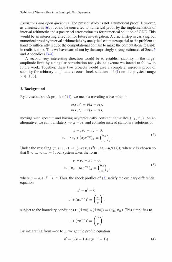
Fig. 1. In (a), we have a graph of g(v) against v for v+ = 1 × 10−4 and γ = 2.0. Note that g(v) dips downbelow zero on the left-hand size. Hence, the energy estimate will not generalize beyond the small-amplituderegime. In (b) we graph the stability boundaries (dark lines) given by (9) and (15), where γ and v+ are thehorizontal and vertical axes, respectively. We see that in our scaling (15) is only a modest improvement over(9). The dotted lines correspond from top to bottom as the parameter regimes for Mach numbers 2, 5, and 10(see the Appendix to see how to determine the Mach number). Hence, this energy estimate does not even holdfor shocks at Mach 2 and γ > 1.084

Using (10) and (11), we abbreviate a few intermediate steps below:

g(v) = − vx

2

[(γ + 1)vγ h(v) − vγ +1h′(v)

h(v)2 +d

d v

[γ vγ−1h(v) − vγ h′(v)

h(v)2 vx

]]

= − vx

2

[vγ

((γ + 1)h(v) − vh′(v)

)

h(v)2 +d

d v

[γ h(v) − vh′(v)

h(v)2 (aγ − h(v))

]]

= −avx vγ−1

2h(v)3 ×[γ 2(γ + 1)vγ +2 − 2(a + 1)γ (γ 2 − 1)vγ +1 + (a + 1)2γ 2(γ − 1)vγ

+ aγ (γ + 2)(γ 2 − 1)v − a(a + 1)γ 2(γ 2 − 1)]

= −avx vγ−1

2h(v)3 [(γ + 1)vγ +2 + vγ (γ − 1)((γ + 1)v − (a + 1)γ

)2 (12)

+aγ (γ 2 − 1)(γ + 2)v − a(a + 1)γ 2(γ 2 − 1)]

≥ −avx vγ−1

2h(v)3 [(γ + 1)vγ +2 + aγ (γ 2 − 1)(γ + 2)v − a(a + 1)γ 2(γ 2 − 1)]

≥ −γ 2a3vx (γ + 1)

2h(v)3v+

⎡⎣

(v

γ +1+

aγ

)2

+ 2(γ − 1)

(v

γ +1+

aγ

)− (γ − 1)

⎤⎦ . (13)

Thus from (9), we have spectral stability. �


We note that the hypothesis in (9) is not sharp. Indeed, one can show from (12), thata stronger condition could be given as

(γ + 1)vγ +2 + vγ (γ − 1)((γ + 1)v − (a + 1)γ

)2 (14)

+aγ (γ 2 − 1)(γ + 2)v − a(a + 1)γ 2(γ 2 − 1) ≥ 0,

which is sharp in the following sense: When this condition fails to be true, then g(v) isno longer nonnegative, and thus the energy method fails. In Fig. 1(a), we see that g(v)

dips on the left-hand side when this inequality is compromised. We remark further thatnear v+, the left-hand side of (14) is monotone increasing in v. Thus, (14) holds if andonly if

(γ + 1)vγ +2+ + v

γ+ (γ − 1) ((γ + 1)v+ − (a + 1)γ )2 (15)

+aγ (γ 2 − 1)(γ + 2)v+ − a(a + 1)γ 2(γ 2 − 1) ≥ 0.

We see from Fig. 1(b) that (15) is only a marginal improvement over (9). However,since (15) is sharp, we cannot hope to prove large-amplitude spectral stability usingthis approach. Instead, we proceed by a combined analytical and numerical approachas in [6–8], first showing that unstable eigenvalues can occur only in a bounded set,then searching for eigenvalues in this set by computing the Evans function numerically.Before doing so, however, we show in the following section that real unstable eigenvaluesdo not exist, even for large-amplitude viscous shocks.

4. No Real Unstable Eigenvalues

In this section we use a novel spectral energy estimate to show that there are no purelyreal unstable eigenvalues for any shock strength. We note that this result is stronger thanthat which could be given by the Evans function stability index (sometimes called theorientation index), which only measures the parity of unstable real eigenvalues, see [4,15,31]. The fact that this holds for all shock strengths is interesting because it is among thestrongest statements about large-amplitude spectral stability that has been proven to date.

Theorem 4.1. Viscous shocks of (1) have no unstable real spectra.

Proof. We multiply (8b) by the conjugate v and integrate along x from ∞ to −∞. Thisgives

∫

R

λuv +∫

R

u′v −∫

R

h(v)v′vvγ +1 =

∫

R

u′′vv

.

Notice that on the real line, λ = λ. Using (8a) to substitute for λv in the first term andfor u′′ in the last term, we get

∫

R

u(u′ − v′) +∫

R

u′v −∫

R

h(v)v′vvγ +1 =

∫

R

(λv′ + v′′)vv

.

Separating terms and simplifying gives∫

R

uu′ + 2∫

R

u′v −∫

R

h(v)v′vvγ +1 = λ

∫

R

v′vv

+∫

R

v′′vv

.


We further simplify by substituting for u′ in the second term and integrating the lastterms by parts to give

∫

R

uu′ + 2∫

R

(λv + v′)v −∫

R

h(v)v′vvγ +1 = λ

∫

R

v′vv

+∫

R

vx

v2 v′v −∫

R

|v′|2v

.

Combining the third and fifth terms using (11) and simplifying, we have∫

R

uu′ + 2λ

∫

R

|v|2 + 2∫

R

v′v − aγ

∫

R

v′vvγ +1 +

∫

R

|v′|2v

= λ

∫

R

v′vv

.

By taking the real part, we arrive at

λ

2

∫

R

(4 − vx

v2

)|v|2 − aγ (γ + 1)

2

∫

R

vx

vγ +2 |v|2 +∫

R

|v′|2v

= 0.

This is a contradiction when λ ≥ 0. �We remark that the absence of positive real eigenvalues limits the admissible onsetof instability to Hopf-like bifurcations where a pair of conjugate eigenvalues crossesthe imaginary axis. In the following section, we give an upper bound on the spectralfrequencies that are admissible. In other words, we show that if a pair of conjugateeigenvalues cross the imaginary axis, they must do so within these bounds.

5. High-Frequency Bounds

In this section, we prove high-frequency spectral bounds. This is an important stepbecause it gives a ceiling as to how far along both the imaginary and real axes that onemust explore for spectrum when doing Evans function computations. Indeed if we wantto check for roots of the Evans function in the unstable half-plane, say using the argumentprinciple, then we need only compute within these bounds. If no roots are found therein,then we have strong numerical evidence that the given shock is spectrally stable. (Indeed,at the expense of further effort, such a calculation may be used as the basis of numericalproof, as described in [6,7].) In this section we show that the high-frequency bounds arequite strong, only allowing unstable eigenvalues to persist in a relatively small triangleadjoining the origin. Moreover, these bounds are independent of the shock amplitude.

Lemma 5.1. The following holds for eλ ≥ 0:

(e(λ) + |�m(λ)|)∫

R

v|u|2 − 1

2

∫

R

vx |u|2 +∫

R

|u′|2

≤ √2

∫

R

h(v)

vγ|v′||u| +

∫

R

v|u′||u|. (16)

Proof. We multiply (8b) by vu and integrate along x . This yields

λ

∫

R

v|u|2 +∫

R

vu′u +∫

R

|u′|2 =∫

R

h(v)

vγv′u.

We get (16) by taking the real and imaginary parts and adding them together, and notingthat |e(z)| + |�m(z)| ≤ √

2|z|. �


Lemma 5.2. The following identity holds for eλ ≥ 0:∫

R

|u′|2 = 2e(λ)2∫

R

|v|2 + e(λ)

∫

R

|v′|2v

+1

2

∫

R

[h(v)

vγ +1 +aγ

vγ +1

]|v′|2, (17)

Proof. We multiply (8b) by v′ and integrate along x . This yields

λ

∫

R

uv′ +∫

R

u′v′ −∫

R

h(v)

vγ +1 |v′|2 =∫

R

1

vu′′v′ =

∫

R

1

v(λv′ + v′′)v′.

Using (8a) on the right-hand side, integrating by parts, and taking the real part gives

e

[λ

∫

R

uv′ +∫

R

u′v′]

=∫

R

[h(v)

vγ +1 +vx

2v2

]|v′|2 + e(λ)

∫

R

|v′|2v

.

The right hand side can be rewritten as

e

[λ

∫

R

uv′ +∫

R

u′v′]

= 1

2

∫

R

[h(v)

vγ +1 +aγ

vγ +1

]|v′|2 + e(λ)

∫

R

|v′|2v

. (18)

Now we manipulate the left-hand side. Note that

λ

∫

R

uv′ +∫

R

u′v′ = (λ + λ)

∫

R

uv′ −∫

R

u(λv′ + v′′)

= −2e(λ)

∫

R

u′v −∫

R

uu′′

= −2e(λ)

∫

R

(λv + v′)v +∫

R

|u′|2.

Hence, by taking the real part we get

e

[λ

∫

R

uv′ +∫

R

u′v′]

=∫

R

|u′|2 − 2e(λ)2∫

R

|v|2.

This combines with (18) to give (17). �Remark 5.3. Lemma 5.2 is a special case of the high-frequency bounds given in [22,31].We also note that (17) follows from a “Kawashima-type” estimate as described in [22,31].

Lemma 5.4. For h(v) as in (7), we have

supv∈[v+,1]

∣∣∣∣h(v)

vγ

∣∣∣∣ = γ1 − v+

1 − vγ+

≤ γ. (19)

Proof. Defining

H(v) := h(v)v−γ = −v + a(γ − 1)v−γ + (a + 1), (20)

we have H ′(v) = −1 − aγ (γ − 1)v−γ−1 < 0 for 0 < v+ ≤ v ≤ v− = 1, hence themaximum of H on v ∈ [v+, v−] is achieved at v = v+. Substituting (5) into (20) andsimplifying yields (19). �

We complete this section by proving our high-frequency bounds.


Theorem 5.5. Any eigenvalue λ of (8) with nonnegative real part satisfies

e(λ) + |�m(λ)| ≤ (√

γ +1

2)2. (21)

Proof. Using Young’s inequality twice on right-hand side of (16) together with (19),we get

(e(λ) + |�m(λ)|)∫

R

v|u|2 − 1

2

∫

R

vx |u|2 +∫

R

|u′|2

≤ √2

∫

R

h(v)

vγ|v′||u| +

∫

R

v|u′||u|

≤ θ

∫

R

h(v)

vγ +1 |v′|2 +(√

2)2

4θ

∫

R

h(v)

vγv|u|2 + ε

∫

R

v|u′|2 +1

4ε

∫

R

v|u|2

< θ

∫

R

h(v)

vγ +1 |v′|2 + ε

∫

R

|u′|2 +

[γ

2θ+

1

4ε

] ∫

R

v|u|2.

Assuming that 0 < ε < 1 and θ = (1 − ε)/2, this simplifies to

(e(λ) + |�m(λ)|)∫

R

v|u|2 + (1 − ε)

∫

R

|u′|2

<1 − ε

2

∫

R

h(v)

vγ +1 |v′|2 +

[γ

2θ+

1

4ε

] ∫

R

v|u|2.

Applying (17) yields

(e(λ) + |�m(λ)|)∫

R

v|u|2 <

[γ

1 − ε+

1

4ε

] ∫

R

v|u|2,

or equivalently,

(e(λ) + |�m(λ)|) <(4γ − 1)ε − 1

4ε(1 − ε).

Setting ε = 1/(2√

γ + 1) gives (21). �In the following section, we do an extensive Evans function study to explore nume-

rically the rest of the right-half plane in an effort to locate the presence of unstablecomplex eigenvalues.

6. Evans Function Computation

In this section, we numerically compute the Evans function to locate any unstable eigen-values, if they exist, in our system. The Evans function D(λ) is analytic to the rightof the essential spectrum and is defined as the Wronskian of decaying solutions of theeigenvalue equation for the linearized operator (8) (see [1,9–13]). In a spirit similar tothe characteristic polynomial, we have that D(λ) = 0 if and only if λ is in the point spec-trum of the linearized operator (8). While the Evans function is generally too complex tocompute explicitly, it can readily be computed numerically, even for large systems [19].


Since the Evans function is analytic in the region of interest, we can numericallycompute the winding number in the right-half plane. This allows us to systematicallylocate roots (and hence eigenvalues) within. As a result, spectral stability can be deter-mined, and in the case of instability, one can produce bifurcation diagrams to illustrateand observe its onset. This approach was first used by Evans and Feroe [13] and hasbeen advanced further in various directions (see for example [2,5–7,19,25,26]).

We begin by writing (8) as a first-order system W ′ = A(x, λ)W , where

A(x, λ) =⎛⎝

0 λ 10 0 1λv λv f (v) − λ

⎞⎠ , W =

⎛⎝

uv

v′

⎞⎠ , ′ = d

dx, (22)

and f (v) = v − v−γ h(v), with h as in (7). Note that eigenvalues of (8) correspondto nontrivial solutions of W (x) for which the boundary conditions W (±∞) = 0 aresatisfied. We remark that since v is asymptotically constant in x , then so is A(x, λ).Thus at each end-state, we have the constant-coefficient system

W ′ = A±(λ)W. (23)

Hence solutions that satisfy the needed boundary condition must emerge from theunstable manifold W −

1 (x) at x = −∞ and the stable manifold W +2 (x) ∧ W +

3 (x) atx = ∞. In other words, eigenvalues of (8) correspond to the values of λ for which thesetwo manifolds intersect, or more precisely, when D(λ) := det(W −

1 W +2 W +

3 )|x=0 is zero.As an alternative, we consider the adjoint formulation of the Evans function

[4,26], where instead of computing the 2-dimensional stable manifold, we find thesingle trajectory W +

1 (x) coming from the unstable manifold of

W ′ = −A(x, λ)∗W (24)

at x = ∞. Note that W +1 (x) is orthogonal to both W +

2 (x) and W +3 (x) since

(W (x)∗W (x))′ = 0 for all x and the initial data of W +1 is orthogonal to that of W +

2and W +

3 . Hence, the original manifolds intersect when W +1 and W −

1 are orthogonal, andtherefore, the adjoint Evans function takes the form D+(λ) := (W +

1 · W −1 )|x=0.

To further improve the numerical efficiency and accuracy of the shooting scheme,we rescale W and W to remove exponential growth/decay at infinity, and thus eliminatepotential problems with stiffness. Specifically, we let W (x) = eµ−x V (x), where µ− isthe growth rate of the unstable manifold at x = −∞, and we solve instead V ′(x) =(A(x, λ) − µ− I )V (x). We initialize V (x) at x = −∞ to be the eigenvector of A−(λ)

corresponding to µ−. Similarly, it is straightforward to rescale and initialize W (x) atx = ∞.

Numerically, we use a finite domain for x , replacing the end states x = ±∞ withx = ±L , for sufficiently large L . Some care needs to be taken, however, to make surethat we go out far enough to produce good results. In Appendices B and C, we explorethe decay rates of the profile v and A(x, λ) and combine our analysis with numericalconvergence experiments to conclude that our domain [−L , L] is sufficiently large. Ourexperiments, described below, were primarily conducted using L = 12, with relativeerror bounds ranging mostly between 10−3 and 10−4. Larger choices of L were neededon the high end of the Mach scale, going up to L = 18 in some cases, to get the relativeerrors down to 10−4. In Table 1, we provide a sample of relative errors in D(λ) forlarge-amplitude shocks.


Table 1. Relative errors in D(λ) are computed by taking the maximum relative error for 60 contour pointsevaluated along the semicircle in Fig. 2(a). Samples were taken for varying L and γ , leaving v+ fixed atv+ = 10−4 (Mach M ≈ 1669). We used L = 8, 10, 12, 14, 16 and γ = 1.2, 1.4, 1.666, 1.8. Relative errorswere computed using the next value of L as the baseline

L γ = 1.2 γ = 1.4 γ = 1.666 γ = 1.8

8 1.23(−1) 1.16(−1) 1.08(−1) 1.04(−1)

10 2.07(−2) 1.46(−2) 1.75(−2) 1.78(−2)

12 2.00(−3) 1.40(−3) 9.85(−4) 7.20(−4)

14 6.90(−4) 5.31(−4) 4.73(−4) 4.71(−4)

We remark also that in order to produce analytically varying Evans function output,the initial data V (−L) and V (L), must be chosen analytically. The method of Kato [20,p. 99], also described in [8], does this well by replacing the eigenvectors of (23) withanalytically defined spectral projectors (see also [5,18]).

Before we can compute the Evans function, we first need to compute the trave-ling wave profile. We use both Matlab’s ode45 routine, which is the adaptive fourth-order Runge-Kutta-Fehlberg method (RKF45), and Matlab’sbvp4c routine, which is anadaptive Lobatto quadrature scheme. Both methods work well and produce essentiallyequivalent profiles.

Our experiments were carried out on the range

(γ, M) ∈ [1, 3] × [1.6, 3000].Recall, for γ ∈ [1, 3], that shocks are known to be stable for M ∈ [1, 1.6], by (15),Sect. 3, hence this completes the study of the range

(γ, M) ∈ [1, 3] × [1, 3000]from minimum Mach number M = 1 far into the hypersonic shock regime, and encom-passing the entire physically relevant range of γ .

For each value of γ , the Mach number M was varied on logarithmic scale with regularmesh from M = 1.6 up to M = 3000. We used 50 mesh points for γ = 1.0 + 0.1k,where k = 1, 2, . . . , 20. For the special values γ = 1.4 and 1.666 (monatomic anddiatomic cases), we did a refined study with 400 mesh points.

For each value of (γ, M), we computed the Evans function along semi-circularcontours that contain the triangular region found in the previous section via ourhigh-frequency bounds; see Fig. 2(a). The ODE calculations for individual λ werecarried out using Matlab’s ode45 routine, which is the adaptive 4th-order Runge-Kutta-Fehlberg method (RKF45), and after scaling out the exponential decay rate of theconstant-coefficient solution at spatial infinity, as described in [5–8,19]. This method isknown to have excellent accuracy [5,19]; in addition, the adaptive refinement gives auto-matic error control. Typical runs involved roughly 300 mesh points, with error toleranceset to AbsTol = 1e-6 and RelTol = 1e-8. Values of λ were varied on a contourwith 60 points. As a check on winding number accuracy, it was tested a posteriori thatthe change in argument of D for each step was less than π/25. Recall, by Rouché’sTheorem, that accuracy is preserved so long as the argument varies by less than π alongeach mesh interval.

In all the cases that we examined, the winding number was zero. This indicatesthat the shocks we considered are spectrally stable, and in view of [21–23], nonlinearstability follows. Moreover, in light of the large Mach numbers considered, this is highlysuggestive of stability for all shock strengths.


(a) (b)

Fig. 2. The graph of the contour and its mapping via the Evans function. In (a), we have a contour, whichis a large semi-circle aligned on the imaginary axis on the right-half plane (horizontal axis real, vertical axisimaginary). In (b) we have the image of the contour mapped by the Evans function. Note that the windingnumber of this graph is zero. Hence, there are no unstable eigenvalues in the semi-circle. Together with thehigh-frequency bounds, this implies spectral stability. Our computation was carried out for γ = 5/3 andv+ = 1 × 10−4. This corresponds to a monatomic gas with Mach number M ≈ 1669 (see Appendix A)

7. Numerical Evolution of Strong Shocks

In this section, we use a standard finite-difference method to simulate perturbedlarge-amplitude viscous shocks, and show that they converge, as expected, to a translateof the original profile.

We do this with a nonlinear Crank-Nicholson scheme with a Newton solver to dealwith the nonlinearity. This method provides second-order accuracy and will allow forlarger time steps than a naive explicit scheme. By differentiating the viscosity term in(3), we have

vt + vx − ux = 0,

ut + ux − aγ v−γ−1vx = uxx

v− uxvx

v2 .

By implementing the Crank-Nicholson averaging, we obtain

vn+1j − vn

j

�t+

1

4�x(vn+1

j+1 − vn+1j−1 + vn

j+1 − vnj−1)

− 1

4�x(un+1

j+1 − un+1j−1 + un

j+1 − unj−1) = 0

and

un+1j − un

j

�t+

1

4�x(un+1

j+1 − un+1j−1 + un

j+1 − unj−1)

− a

4�xγ (vn

j )−γ−1(vn+1

j+1 − vn+1j−1 + vn

j+1 − vnj−1)

− 1

2(�x)2vnj(un+1

j+1 − 2un+1j + un+1

j−1 + unj+1 − 2un

j + unj−1)


Fig. 3. Snapshots of the evolution of a perturbed viscous shock wave solution generated by our extendedCrank-Nicholson scheme (top curve: v against x ; bottom curve: u against x , with time t fixed and increasingfrom figure to figure). The parameters used were γ = 1.4 and v+ = 9 × 10−6. This corresponds to a diatomicgas with Mach number M ≈ 2877 (see Appendix A). As expected, the wave converges to a translate of theoriginal shock

+1

16(�x)2(vnj )

2 (un+1j+1 − un+1

j−1 + unj+1 − un

j−1)

×(vn+1j+1 − vn+1

j−1 + vnj+1 − vn

j−1) = 0,

where n and j are, respectively, the discretized temporal and spacial indices.To cope with the nonlinearities, we use the Newton solver

(U n+1

V n+1

)

k+1=

(U n+1

V n+1

)

k−

(Du F Dv FDuG DvG

)−1

k,

(F(U n+1, V n+1)

G(U n+1, V n+1)

)

k,

where F(U n+1, V n+1) and G(U n+1, V n+1) are the above finite difference schemes, andDu F , Dv F , DuG, and DvG are their corresponding partial derivatives. Hence, we usethe previous time step as our initial guess in Newton’s method and then iterate untilconvergence.

In Fig. 3, we see the evolution of a perturbed viscous shock of extremely high Machnumber. We used a perturbation with a positive mass so that we could observe theconvergence to a translate of the original profile, thus numerically demonstrating non-linear stability. We remark that perturbed profiles as predicted by the nonlinear theory[22,23] exhibit also a “diffusion wave”, or approximate Gaussian signal, of constant


mass, leaving the shock wave on the right and convecting with outgoing characteristicspeed, which absorbs the portion of the mass not accounted for by shock shift. Thisis clearly visible for small- or intermediate-amplitude shocks, but for large-amplitudeshocks travels with characteristic speed ∼ v

−1/2+ → +∞, leaving the viewing frame

essentially instantaneously.

Appendix A. Mach Number for the p-System

The Mach number is defined as

M = u+ − σ

c+,

where u+ is the downwind velocity, σ is the shock speed, and c+ is the downwind soundspeed, all in Eulerian coordinates. By considering the conservation of mass equation,we have ρt + (ρu)x = 0. Hence, the jump condition is given by σ [ρ] = [ρu], whichimplies, in the original scaling for (1), that

σ = u+v− − u−v+

v− − v+.

Hence,

M = u+ − σ

c+= v+(u− − u+)

c+(v− − v+)= v+[u]

c+[v] = −sv+

c+

or

M2 =(

u+ − σ

c+

)2

= s2v2+

−p′(v+)= s2v2

+

γ a0v−γ−1+

= vγ +3+

γ

s2

a0.

To express this in our scaling, which is given in (3), we need to swap the pluses andminuses. Noting that 0 < v+ < v− = 1, we simplify to get

M2 = 1

γ vγ+

1 − vγ+

1 − v+= 1

γ a.

Recalling that a ∼ vγ+ as v+ → 0, we find that

v+ ∼ (γ M2)− 1

γ (25)

as M → ∞. In particular,

| log v+| ∼ γ −1(log γ + 2 log M). (26)


Appendix B. Profile Bounds

Denote profile equation (4) as v′ = H(v, v+) := v(v − 1 + a(v−γ − 1)).

Lemma B.1. For γ ≥ 1, 0 ≤ x < 1,

1 ≤ 1 − xγ

1 − x≤ γ. (27)

Proof. By convexity of f (x) = xγ , the difference quotient (27) is increasing in x ,bounded above by f ′(1) = γ , and below by its value at x = 0. �Proposition B.2. For γ ≥ 1 and v+ ≤ v ≤ 1

6 , v+ ≤ 112 ,

− γ (v − v+) ≤ H(v, v+) ≤ −3

4(v − v+). (28)

For γ ≥ 1, v+ ≤ 14γ

, and 34 ≤ v ≤ v− = 1,

1

2(v − v−) ≤ H(v, v+) ≤ (v − v−). (29)

Proof. By (5),

H(v, v+) = v((v − 1) − (v+ − 1)(v−γ − 1)

v−γ+ − 1

)

= v((v − v+) +

( 1 − v+

1 − vγ+

)((v+

v

)γ − 1))

= (v − v+)(v −

( 1 − v+

1 − vγ+

)(1 − (v+v

)γ

1 − (v+v

)))

.

Applying (27) with x = v+v

, we obtain (28) from

v − γ ≤ H(v, v+)

v − v+≤ v − (1 − v+).

Similarly, we may obtain (29) by the calculation

H(v, v+)

v − 1= v

(1 −

(v+

v

)γ ( 1 − v+

1 − vγ+

)(1 − vγ

1 − v

))≥ v − γ v+ ≥ 3

4− 1

4.

�Corollary B.3. For γ ≥ 1, 0 < v+ ≤ 1

12 , and v(0) := v+ + 112 , the solution v of (4)

satisfies

|v(x) − v+| ≤( 1

12

)e− 3x

4 x ≥ 0, (30a)

|v(x) − v−| ≤(1

4

)e

x+122 x ≤ 0. (30b)


Proof. Observing that (v − v+)(0) = 112 , we obtain (30a) by Proposition B.2 and the

comparison principle for first-order scalar ODE. Likewise, (30b) follows by (29) togetherwith the observation that, by convexity of H , |H | is bounded below by estimates obtainedat v = v+ + 1

12 and v = 34 of 1

16 and 18 , respectively, so that v traverses [v+ + 1

12 , 34 ] over

an x-interval of length ≤ 3/41/16 = 12. �

Remark B.4. From Proposition B.2 and Corollary B.3, we obtain the remarkable factthat, in the scaling we have chosen, v decays up to first derivative to endstates v± at auniform exponential rate independent of shock strength, despite the apparent singularityat v = v+.

Appendix C. Initialization Error

Lemma C.1. For A as in (22), | · | the Euclidean (�2) matrix operator norm,

|A(x, λ) − A+(λ)| ≤(2|λ| + 1 + γ 2(γ − 1)v−1

+

12

)e− 3x

4 , x ≥ 0, (31a)

|A(x, λ) − A−(λ)| ≤(2|λ| + 1 + 2γ 3(γ − 1)

4

)e

x+122 , x ≤ 0. (31b)

Proof. By (22), |A(x, λ)− A±(λ)| ≤ 2λ|v −v±|+ | f (v)− f (v±)|. As computed in theproof of Lemma 5.4, f ′(v) = −1 − aγ (γ − 1)v−γ−1. Applying (27) to the expressionfor a in (5), we obtain v

γ+ ≤ a ≤ γ v

γ+ , so that

| f ′(v)| ≤ 1 + γ 2(γ − 1)v−1 ≤ 1 + γ 2(γ − 1)v−1+ ,

yielding (31a) by the Mean Value Theorem and (30a). Bound (31b) follows similarly. �Theorem C.2. (Simplified Gap Lemma [6,7,15]) Let V + and µ+ be a left eigenvectorand associated eigenvalue of −A+(λ) and suppose that

|e(−A+−µ+)x | ≤ C1e−ηx x ≤ 0,

|(A − A+)(x)| ≤ C2e−ηx x ≥ 0,(32)

with 0 ≤ η < η. Then, there exists a solution W = eµ+x V (x, λ) of (24) with

|V (x, λ) − V +(λ)||V +(λ)| ≤ C1C2e−ηx

(η − η)(1 − ε)x ≥ L (33)

provided (η−η)−1C1C2e−ηL ≤ ε. Similar estimates hold for solutions of (22) on x ≤ 0.

Proof. Writing V ′ = V (−A+ − µ+) + V (−A + A+) and imposing the limiting behaviorV (+∞, λ) = V +, we obtain by Duhamel’s Principle,

V (x) = V + −∫ +∞

xV (y)e(−A+−µ+)(x−y)(A − A+)dy,

from which the result follows by a straightforward Contraction Mapping argument using(32). See [6,7,15] for details. �


Lemma C.3. For λ satisfying (21), γ ∈ [1, 3], and v+ ≤ 112 , (32)(a) holds with

η = 1/2γ , η = 1/4γ , and C1 = 104, and similarly for x ≤ 0.

Proof. Using the inverse Laplace transform representation

e(−A+−µ+)x = 1

2π i

∮

ezt (z + A+ + µ+)−1dz,

where is a contour enclosing the eigenvalues of (−A+ − µ+) and distance η away, andestimating the resolvent norm |(z + A+ + µ+)−1| by Kramer’s rule, we obtain the statedcrude bound, and similarly for x ≤ 0. �

For error tolerance θ := 10−k (| log θ | ∼ 2k), define

L−(θ) := 2(| log 10−4| + | log(2γ + 7 + 2γ 3(γ − 1))| + | log θ |

)+ 12,

L+(θ, v+) := 4

3

(| log 10−4| + | log(2γ + 7 + γ 2(γ − 1)v−1

+ )| + | log θ |).

Corollary C.4. For λ satisfying (21), we have relative error bounds

|W −1 (−L−, λ) − V −eµ−x |

|V −eµ−x | ,|W +

1 (L+, λ) − V +eµ+x ||V +eµ+x | ≤ θ. (34)

Proof. This follows by (33) with (31), Lemma C.3, and (21). �Remark C.5. Combining (34) with (26), we find that

L+ ∼ 4

3(2 log M + 4 + | log 10−4| + | log θ |)

suffices to obtain relative initialization error less than θ for γ ∈ [1, 3] and λ in thecomputational region (21). For θ = 10−3, we thus obtain θ tolerance up to M = 3, 000 ∼103 for L+ ∼ 40. This is conservative, as we have made little effort to optimize bounds,but still within the realm of our experiments. Our numerical convergence studies indicatethat L± = 18 in fact suffices for 10−3 accuracy.

References

1. Alexander, J., Gardner, R., Jonesm, C.: A topological invariant arising in the stability analysis of travellingwaves. J. Reine Angew. Math. 410, 167–212 (1990)

2. Alexander, JC, Sachs, R.: Linear instability of solitary waves of a Boussinesq-type equation: a computerassisted computation. Nonlinear World 2(4), 471–507 (1995)

3. Batchelor, G.K.: An introduction to fluid dynamics. Cambridge Mathematical Library. Cambridge:Cambridge University Press, paperback edition, 1999

4. Benzoni-Gavage, S., Serre, D., Zumbrun, K.: Alternate Evans functions and viscous shock waves. SIAMJ. Math. Anal. 32(5), 929–962 (electronic) (2001)

5. Bridges, T.J., Derks, G., Gottwald, G.: Stability and instability of solitary waves of the fifth-order KdVequation: a numerical framework. Phys. D 172(1–4), 190–216 (2002)

6. Brin, L.Q.: Numerical testing of the stability of viscous shock waves. PhD thesis, Indiana University,Bloomington, 1998

7. Brin, L.Q.: Numerical testing of the stability of viscous shock waves. Math. Comp. 70(235),1071–1088 (2001)


8. Brin, L.Q., Zumbrun, K.: Analytically varying eigenvectors and the stability of viscous shock waves.In: Seventh Workshop on Partial Differential Equations, Part I (Rio de Janeiro, 2001), P.L. Dias,D. Marchesin, A. Nelson, C. Tomei, eds. Mat. Contemp. 22, 19–32, (2002)

9. Evans, J.W.: Nerve axon equations. I. Linear approximations. Indiana Univ. Math. J. 21, 877–885 (1971)10. Evans, J.W.: Nerve axon equations. II. Stability at rest. Indiana Univ. Math. J. 22, 75–90 (1972)11. Evans, J.W.: Nerve axon equations. III. Stability of the Nerve Impulse. Indiana Univ. Math. J. 22,

577–593 (1972)12. Evans, J.W.: Nerve axon equations. IV. The stable and the unstable impulse. Indiana Univ. Math.

J. 24(12), 1169–1190 (1974)13. Evans, J.W., Feroe, J.A.: Traveling waves of infinitely many pulses in nerve equations. Math.

Biosci. 37, 23–50 (1977)14. Gardner, R., Jones, C.K.R.T.: A stability index for steady state solutions of boundary value problems for

parabolic systems. J. Differ. Eqs. 91(2), 181–203 (1991)15. Gardner, R.A., Zumbrun, K.: The gap lemma and geometric criteria for instability of viscous shock

profiles. Comm. Pure Appl. Math. 51(7), 797–855 (1998)16. Goodman, J.: Nonlinear asymptotic stability of viscous shock profiles for conservation laws. Arch. Rat.

Mech. Anal. 95(4), 325–344 (1986)17. Howard, P., Zumbrun, K.: Pointwise estimates and stability for dispersive-diffusive shock waves. Arch.

Rat. Mech. Anal. 155(2), 85–169 (2000)18. Humpherys, J., Sandstede, B., Zumbrun, K.: Efficient computation of analytic bases in Evans function

analysis of large systems. Numer. Math. 103(4), 631–642 (2006)19. Humpherys, J., Zumbrun, K.: An efficient shooting algorithm for evans function calculations in large

systems. Physica D 220(2), 116–126 (2006)20. Kato, T.: Perturbation theory for linear operators. Classics in Mathematics. Berlin: Springer-Verlag,

1995 (Reprint of the 1980 edition)21. Mascia, C., Zumbrun, K.: Pointwise Green function bounds for shock profiles of systems with real

viscosity. Arch. Rat. Mech. Anal. 169(3), 177–263 (2003)22. Mascia, C., Zumbrun, K.: Stability of large-amplitude viscous shock profiles of hyperbolic-parabolic

systems. Arch. Rat. Mech. Anal. 172(1), 93–131 (2004)23. Mascia, C., Zumbrun, K.: Stability of small-amplitude shock profiles of symmetric hyperbolic-parabolic

systems. Commun. Pure Appl. Math. 57(7), 841–876 (2004)24. Matsumura, A., Nishihara, K.: On the stability of travelling wave solutions of a one-dimensional model

system for compressible viscous gas. Japan J. Appl. Math. 2(1), 17–25 (1985)25. Pego, R.L., Smereka, P., Weinstein, M.I.: Oscillatory instability of traveling waves for a KdV-Burgers

equation. Phys. D 67(1–3), 45–65 (1993)26. Pego, R.L., Weinstein, M.I.: Eigenvalues, and instabilities of solitary waves. Philos. Trans. Roy. Soc.

London Ser. A 340(1656), 47–94 (1992)27. Smoller, J.: Shock waves and reaction-diffusion equations. New York: Springer-Verlag, Second edition,

199428. Texier, B., Zumbrun, K.: Relative Poincaré-Hopf bifurcation and galloping instability of traveling waves.

Methods Appl. Anal. 12(4), 349–380 (2005)29. Texier, B., Zumbrun, K.: Galloping instability of viscous shock waves. http://arxiv.org/list/math.Ap/

0609331, 200630. Texier, B., Zumbrun, K.: Hopf bifurcation of viscous shock waves in compressible gas- and magnetohy-

drodynamics. Toappear Arch. Rat. Mech. Anal., doi:10.1007/s00205-008-0012-x31. Zumbrun, K.: Multidimensional stability of planar viscous shock waves. Lecture notes, TMR summer

school, 199932. Zumbrun, K., Howard, P.: Pointwise semigroup methods and stability of viscous shock waves. Indiana

Univ. Math. J. 47(3), 741–871 (1998)

Communicated by P. Constantin

http://arxiv.org/list/math.Ap/0609331

http://arxiv.org/list/math.Ap/0609331

http://dx.doi.org/10.1007/s00205-008-0012-x

Documents

Stability of Viscous Shocks in Isentropic Gas Dynamicsjeffh/publications/papers/BHRZ.pdfDigital Object Identiﬁer (DOI) 10.1007/s00220-008-0487-4 Commun. Math. Phys. Communications