TTS From Zero

Building Synthetic Voices for New Languages

John Kominek

CMU-LTI-09-006

Language Technologies Institute

School of Computer Science

Carnegie Mellon University

Submitted in partial fulfillment of the requirements

of the degree of Doctor of Philosophy.

Thesis Committee:

Alan W Black (chair)

Tanja Schultz

Alexander I. Rudnicky

Richard W. Sproat (University of Illinois at Urbana-Champaign)

Copyright© John Kominek

Abstract

A developer wanting to create a speech synthesizer in a new voice for an under-resourced

language faces hard problems. These include difficult decisions in defining a phoneme set and a

laborious process of accumulating a pronunciation lexicon. Previously this has been handled

through involvement of a language technologies expert. By definition, experts are in short supply.

The goal of this thesis is to lower barriers facing a non-technical user in building “TTS from

Zero.” Our approach focuses on simplifying the lexicon building task by having the user listen to

and select from a list of pronunciation alternatives. The candidate pronunciations are predicted by

grapheme-to-phoneme (G2P) rules that are learned incrementally as the user works through the

vocabulary. Studies demonstrate success for Iraqi, Hindi, German, and Bulgarian, among others.

We compare various word selection strategies that the active learner uses to acquire maximally

predictive rules.

Incremental G2P learning enables iterative voice building. Beginning with 20 minutes of

recordings, a bootstrapped synthesizer provides pronunciation examples for lexical review, which

is fed into the next round of training with more recordings to create a larger, better voice... and so

on. Voice quality is measured through transcription on heldout sentences, AB listening tests, and

through mel cepstral distortion (MCD). We have discovered a log-linear law relating corpus size

to mel cepstral distortion, and measured the gain attributed to a better lexicon. Data also supports

a log-linear relation between MCD and AB listening tests, thereby grounding the most commonly

used objective measure to the easiest form of subjective evaluation.

Finally, we introduce a novel approach to inferring a lexicon directly from acoustic samples

recorded by the user. Our algorithm combines evidence provided by an all-phone decoder with

synthesizer output to discover accurate as-spoken surface pronunciations.

iii

iv

Acknowledgments

The road to a Doctorate is long and winding and bumpy, and would be impossible were it not for

the people met along the way. This is true of my advisor Alan W Black. Always cheerful and

enthusiastic, ever eager to show you his latest work and to encourage yours, Alan is unequaled in

his willingness to provide research opportunities and to offer his support – not the least of which

by writing ever more Festival code – so that his students can work at the forefront of the field. No

one knows text-to-speech like Alan does. I can only hope to have absorbed a fraction of that

knowledge by sheer din of exposure.

Tanja Schultz was hugely beneficial by initiating and directing the SPICE project. The

opportunity provided by this project constitutes the core of my dissertation, and I am forever

indebted to the students that took the “SPICE course” as the lab in Multilingual Speech-to-Speech

Translation came to be called. Working with Matt Hornyak and Sameer Badaskar to get it all

working was an unforgettable experience. Tanja also deserves thanks for attending my pre-

proposal talks, as well as reading through my proposal and dissertation to provide constructive

criticism. As do my other committee members, Alex Rudnicky and Richard Sproat. Thank you.

Through his steady guidance and decades of experience, Richard Stern helped this thesis along

more than he realizes. InterSpeech 2006 was the highlight of my time at CMU, and would never

have come together without his total commitment and orchestration of the steering committee.

Even more important perhaps was the supportive atmosphere present at our weekly SphinxLunch

meetings, an atmosphere directly reflective of Rich's personality. Many interesting discussions

occurred in these meetings, but the willingness of Ravi Mosur, Arthur Chan, and David Huggins-

Danes to explain the inner workings of Sphinx stands out. Dan Bohus and Antoine Raux engaged

in great dialogs about dialog systems. As a visiting researcher several years ago, Marelie Davel

was a frequent SphinxLunch participant and influenced the direction of my research more than I

ever anticipated.

I'd like to thank everyone who has ever recorded the Arctic prompt list, or will do so in the

future. Especially the original Arctic voices: awb, bdl, clb, rms, slt. I am more well known due to

their patience in the recording booth than to all other factors combined. Bano Banerjee allowed

me to record every one of his Bengali phonemes and gamely let me scrutinize his speech in

public. Due to him the conundrum of four-way stop consonant contrasts is a “solved mystery.”

v

Alan Black and Keiichi Tokuda initiated the Blizzard Challenge. The Challenge owes to me its

name and innumerable hours of lost sleep. It was an irreplaceable learning experience.

Ian Lane and Jamal Al-Shami were of great help in the Transtac project. In our local synthesis

group I often found recourse to chat with Arthur Toth, Brian Langner, and Kishore Prahallad – as

well as trade pleadings for listening tests. Tina Bennett organized the speech synthesis reading

group. Guest appearances by Kornel Laskowski made me wonder why he isn't in TTS. Stan Jou

should have been in TTS the way he was willing to have his face wired up with electrodes.

Before returning to Japan, Heiga Zen and Tomoki Toda inspired us with their breakthrough work.

I had the privilege of sharing office space with some great people, including Kevin Collins-

Thompson, Vasco Calias Pedro, Alicia Tribble, Joy (who has a real name but we never called him

by it, whatever it is), Yan Liu, Chad Langley, Ben Han, Ariadna Font Llitjos, Rashmi

Gangadharaiah, and Jonathan Elsas. In the course of our department's annual seating rotation,

Kathrin Probst always seemed to occupy the same desk one season ahead of me. I liked visiting

her and Guy Lebanon to find out where I'd end up next. Paul Ogilvie lived just one door (or one

floor) away and was always inviting.

It was a delight to replace the big water bottles in the LTI kitchen for June Sison. I woke up in

the morning looking forward to an “H2O alert” in my inbox.

On the topic of replenishing vital fluids, I thank the celebrated SCS coke machine. Whenever

my research was going poorly I never failed to find a sense of accomplishment in the simple act

of refilling bottles. Besides, when it was jammed, and I was thirsty, you can't beat having the key.

Jie Yang played the role of surrogate advisor during my early years. From him I learned how

research is done at CMU. Monika Woszczyna helped me debug PeopleTracker at 2 a.m. in the

morning by tossing Ratbert across the room and making the software believe that she is a chair.

Rick Kazman, having been through it all before and survived, provided an understanding ear

when it was needed most. Jorge Cham provided comic relief – plus an autograph to go with it.

My Mother has stuck through it all, urging me to “keep your stick on the ice.” She was more

nervous on the day of my defense than I was. And I was nervous. My nephew Jakob Koblinski,

who was born around the time I began the PhD program, has been my external measure of what

1st year through nth year status really means.

Most of all, I can barely express gratitude to my wonderful wife for all her support. fff

vi

in memory of

Rudy P. Kominek

1927-2000

vii

viii

Table of Contents

1 Introduction......................................................................................................................1

1.1 Motivation and context.........................................................................................................3

1.2 Application and assumptions................................................................................................5

1.2.1 Technical limitations.....................................................................................................7

1.3 Design objectives..................................................................................................................7

1.4 Thesis statement....................................................................................................................8

1.5 Organization of thesis.........................................................................................................10

2 Background....................................................................................................................13

2.1 The synthesis pipeline.........................................................................................................13

2.2 The role and challenge of phonemes..................................................................................16

2.2.1 Definition of terms .....................................................................................................16

2.2.2 The International Phonetic Alphabet (IPA).................................................................18

2.2.3 The GlobalPhone corpus and phone set .....................................................................19

2.2.4 Polyglot multiphone databases...................................................................................20

2.2.5 The paucity of defined phoneme sets.........................................................................21

2.2.6 The design freedom of phoneme sets.........................................................................23

2.3 Pronunciation modeling in speech synthesis......................................................................25

2.3.1 Phonemes as a mediating layer...................................................................................28

2.4 Possible solutions................................................................................................................29

2.4.1 Strengths and weaknesses of possible solutions.........................................................31

2.4.2 Applicability of approaches........................................................................................32

2.5 Related work.......................................................................................................................33

2.6 Connection to rest of thesis.................................................................................................35

3 G2P Rules......................................................................................................................37

3.1 Some approaches to G2P conversion..................................................................................38

3.1.1 High level rule chains – the handwritten Wasser dictionary......................................40

3.1.2 Low level rule chains – machine learned...................................................................42

3.1.3 CART tree rules..........................................................................................................44

3.1.4 Accuracy and prediction entropy................................................................................50

3.1.5 Rule system entropy versus prediction entropy..........................................................51

ix

3.1.6 Multiple pronunciation prediction..............................................................................53

3.1.6.1 Method 1 – leaf node emission probabilities......................................................53

3.1.6.2 Method 2 – complete rule chain traversal..........................................................54

3.1.7 Reweighting with phone transition probabilities .......................................................55

3.1.8 Rule learning architectures: pros and cons.................................................................57

3.2 G2P rule learning................................................................................................................58

3.2.1 Formal definition of G2P rules...................................................................................59

3.2.2 G2P symbol alignment................................................................................................62

3.2.3 Search strategy for rule learning.................................................................................65

3.2.4 Rule expansion algorithm...........................................................................................68

3.2.5 Learning algorithm speed...........................................................................................70

3.3 G2P performance across languages....................................................................................71

3.3.1 A test suite of eight languages....................................................................................71

3.3.2 Empirical measurements.............................................................................................72

3.4 Active learning and word ordering....................................................................................81

3.4.1 Word selection strategies............................................................................................82

3.4.2 Algorithm description.................................................................................................84

3.4.3 Active learner performance.........................................................................................85

3.4.3.1 Why active learning is inherently limited...........................................................87

3.4.4 Token weighted word selection..................................................................................87

3.5 Connection to rest of thesis.................................................................................................89

4 Field Studies...................................................................................................................91

4.1 Speech-to-Speech System Description...............................................................................93

4.2 Provided lexical resources..................................................................................................94

4.2.1 Reference lexicon.......................................................................................................95

4.2.2 Transtac Iraqi Names Collection database..................................................................96

4.2.3 Other data resources...................................................................................................97

4.3 Task descriptions.................................................................................................................98

4.4 Orthography, transliteration, phonetics, and vowelization of Iraqi Arabic.........................99

4.4.1 G2P complexity of Arabic in brief............................................................................100

4.4.2 Iraqi Arabic phoneme inventory and phonology......................................................101

4.4.3 Iraqi Arabic vowel system........................................................................................104

x

4.4.4 Acoustic correlates of emphatic versus non-emphatic /s/.........................................106

4.4.5 Modern Standard Arabic writing system..................................................................107

4.4.6 Grapheme to phoneme relationship..........................................................................113

4.4.6.1 G2P rules applied to vowelized words.............................................................115

4.4.6.2 P2P rules from Arabic to English.....................................................................116

4.4.6.3 Cross-word interaction affecting pronunciation...............................................117

4.5 Lexicon verification using native speakers.......................................................................117

4.5.1 Application user interface.........................................................................................117

4.5.2 Measurement protocol..............................................................................................121

4.5.3 Human efficiency measurements..............................................................................122

4.5.4 Typical usage patterns...............................................................................................125

4.5.5 Comparison to the literature.....................................................................................128

4.5.6 Improvement in ASR word error rate.......................................................................129

4.6 Summary...........................................................................................................................130

5 Voices From Little Data..............................................................................................131

5.1 Effect of CART tree training conditions on MCD............................................................134

5.1.1 Experimental data and testing protocol....................................................................135

5.1.1.1 Database selection............................................................................................135

5.1.1.2 Training / testing data split...............................................................................135

5.1.1.3 Resynthesis and measurement..........................................................................136

5.1.1.4 Variation of experimental conditions................................................................136

5.1.2 Feature importance in CART tree training...............................................................136

5.1.2.1 Feature importance by class / influence of stop value......................................139

5.1.3 Effect of context width.............................................................................................142

5.1.4 Position features and a minimal training set.............................................................144

5.1.5 Effect of Database size ............................................................................................146

5.2 MCD-based calibration using English..............................................................................147

5.2.1 Effect of not having a lexicon for English................................................................148

5.2.2 Evaluating languages other than English..................................................................149

5.3 Iterative voice development..............................................................................................152

5.3.1 Transcription tests.....................................................................................................154

5.3.2 MCD measurements.................................................................................................155

xi

5.4 Objective-subjective score correlation..............................................................................156

5.4.1 A-B preference tests..................................................................................................157

5.4.2 Ratings from A-B preference results........................................................................158

5.4.3 Relation between ratings and transcription accuracy...............................................159

5.4.4 Relation between ratings and MCD..........................................................................160

5.4.5 Relation between ratings and database size..............................................................161

5.4.6 Best use of effort – larger lexicon or more speech?.................................................162

5.5 Summary...........................................................................................................................163

6 Pronunciations From Acoustics...................................................................................165

6.1 Automatic lexicon inference – description.......................................................................166

6.1.1 Definition of Terms...................................................................................................167

6.1.1.1 Data Components.............................................................................................167

6.1.1.2 Model Component Initialization.......................................................................171

6.1.1.3 Initial Model Testing.........................................................................................172

6.2 Lexical inference from acoustics......................................................................................173

6.2.1.1 Minimum distortion hypothesis as best............................................................174

6.2.2 Inner Iterative Loop – Lexicon update.....................................................................175

6.2.2.1 Lexicon inference – discrete-only versus discrete+continuous........................178

6.2.2.2 Word extraction from phonetic decodings........................................................179

6.2.2.3 Iterative Model Update.....................................................................................180

6.3 Middle Iterative Loop – Phoneset Inference.....................................................................181

6.3.1 Split operations.........................................................................................................182

6.3.2 Assign operations......................................................................................................183

6.3.3 Merge operations......................................................................................................183

6.3.4 Split/assign/merge policy..........................................................................................183

6.3.4.1 Bottom-up agglomerative clustering................................................................184

6.3.5 Phoneme Inference Flowchart..................................................................................185

6.4 Lexicon Inference from Acoustics..................................................................................186

6.4.1 Phoneme decoder model tuning................................................................................186

6.4.2 Grapheme decoder parameter exploration................................................................192

6.4.3 Examples of inferred pronunciations in English......................................................194

7 Conclusions..................................................................................................................199

xii

7.1 Contributions....................................................................................................................199

7.1.1 G2P Rules.................................................................................................................199

7.1.2 User studies...............................................................................................................200

7.1.3 MCD Calibration......................................................................................................200

7.1.4 Iterative voice building.............................................................................................201

7.1.5 Correlating objective to subjective quality measures...............................................202

7.1.6 Lexicon inference from acoustics.............................................................................202

7.2 Future Work......................................................................................................................203

8 Appendix A – CART training features.........................................................................205

9 Appendix B – Bradly-Terry Models............................................................................209

9.1 Basics of rating systems....................................................................................................211

9.2 Relation to pythagorean sabermetrics...............................................................................215

9.3 Relation to Gaussian random processes............................................................................218

9.4 Direct maximum likelihood estimate................................................................................224

9.5 Unbiased two-player estimator.........................................................................................226

9.6 Bayesian prior of unbiased estimator................................................................................231

9.7 Bayesian prior with many players....................................................................................235

9.7.1 Applying player-specific priors................................................................................237

9.8 Minorization-Maximization and general EM update........................................................238

9.8.1 Small numerical example.........................................................................................240

10 Appendix C – Acoustically Inferred Pronunciations.................................................245

11 Appendix D – The Three Laws of Disserosophy.......................................................255

12 Bibliography..............................................................................................................257

xiii

Index of Tables

Table 1.1 Distribution of speaker population of the world's languages............................................4

Table 1.2 Design objectives for voice construction software...........................................................8

Table 2.1 Processing stages of Festival synthesizer........................................................................14

Table 2.2 Activities of each processing stage by level of user expertise........................................15

Table 2.3 The IPA consonant, vowel and diacritic charts...............................................................19

Table 2.4 Composition of polyglot diphone databases...................................................................21

Table 2.5 A selection of 28 most populous languages of India.......................................................22

Table 2.6 Difference in English vowel sets between different dictionaries....................................25

Table 2.7 Five levels of labeling typology......................................................................................26

Table 2.8 TIMIT-based allophone of Miller's post-lexical rules.....................................................28

Table 2.9 Options for bootstrapping a phoneme set and pronunciation dictionary........................30

Table 2.10 English ASR results of Singh and Raj experiments on phoneme splitting...................35

Table 2.11 Comparison of seven approaches for lexicon and synthesizer development................36

Table 3.1 Distribution of rules in Wasser G2P system....................................................................40

Table 3.2 Wasser rules for the letter p.............................................................................................41

Table 3.3 Predefined contexts in Wasser rule system.....................................................................41

Table 3.4 Performance of Wasser rules for letter p on eight example words..................................42

Table 3.5 Percentage of words with n prediction errors using Wasser rules...................................42

Table 3.6 Rule chain covering the productions of the letter p example..........................................43

Table 3.7 Performance of CART tree rule systems on letter p example.........................................51

Table 3.8 Performance of rule chains on letter p example..............................................................51

Table 3.9 System entropy versus production entropy for CART trees...........................................52

Table 3.10 System entropy versus production entropy for rule chains...........................................52

Table 3.11 Predicted probabilities of the word “philip”.................................................................54

Table 3.12 Weighted probabilities of the letter p in “stephen”.......................................................55

Table 3.13 Combination of phone prediction likelihoods and language model likelihoods...........56

Table 3.14 Small lexicon with annotations.....................................................................................59

Table 3.15 Cell visitation pattern of minimum-length mismatch ordering.....................................64

Table 3.16 Example words from the cell visitation pattern............................................................64

Table 3.17 Letter contexts of two example words..........................................................................65

xiv

Table 3.18 Some candidate contexts for explaining p → /f/...........................................................67

Table 3.19 Some more candidate contexts for explaining p → /f/..................................................68

Table 3.20 Number of G2P rules for five languages.......................................................................73

Table 3.21 Summary statistics for four langauges..........................................................................74

Table 3.22 Power law fit to the growth of G2P system size...........................................................76

Table 3.23 Comparison of rule system growth for Italian..............................................................77

Table 3.24 Perplexity measures for six languages..........................................................................78

Table 4.1 Counts of named entity words by category.....................................................................97

Table 4.2 Arabic consonant inventory...........................................................................................102

Table 4.3 Iraqi Arabic consonant phoneset used in CMU Transtac system..................................103

Table 4.4 Occurrence count of geminated consonants per phoneme............................................103

Table 4.5 Measurements contrasting formant positions of emphatic and non-emphatic /s/.........106

Table 4.6 Simplified verbal case system illustrating Arabic root and template construction.......108

Table 4.7 Related Arabic glyphs...................................................................................................110

Table 4.8 Iraqi Arabic consonant graphemes................................................................................111

Table 4.9 Iraqi vowels with diacritic modification.......................................................................112

Table 4.10 Iraqi Arabic consonant graphemes..............................................................................113

Table 4.11 Distribution of diacritic marks in LDC Iraqi Arabic dictionary..................................114

Table 4.12 Example illustrating root and template filling.............................................................115

Table 4.13 Second example illustrating root and template filling................................................116

Table 4.14 Hand-written rules to transform Iraqi to English phonesets.......................................116

Table 4.15 Timing statistics per word of lexicon reviewers, selection case.................................123

Table 4.16 Linear regression fit of reviewer timing statistics.......................................................123

Table 4.17 Timing statistics per word of lexicon reviewers, type-in case....................................125

Table 4.18 Most common patterns of wavefile play sequences....................................................127

Table 4.19 Play ratio and selection percentages of pronunciations by position...........................128

Table 4.20 Effect of updated lexicon on ASR word error rates....................................................129

Table 5.1 Four feature classes and number of features per class..................................................138

Table 5.2 Predictive ability and ranking of position feature classes.............................................145

Table 5.3 Change in MCD as size of database doubles................................................................147

Table 5.4 Word transcription accuracy for 24 German test sentences..........................................151

Table 5.5 Word transcription accuracy for 24 Hindi test sentences..............................................151

Table 5.6 Size and recording time of prompts for incremental voice...........................................152

xv

Table 5.7 Five iterations of lexicon expansion.............................................................................152

Table 5.8 Average time spent on lexicon per expansion stage......................................................152

Table 5.9 Distribution of lexicon selection choices per expansion stage......................................153

Table 5.10 Transcription error counts for incremental voice build...............................................154

Table 5.11 Improvement in MCD as extra utterances are recorded and lexicon expanded..........155

Table 5.12 Average time to perform AB-tie listening tests...........................................................157

Table 5.13 Winning probabilities between two players having a given rating difference............158

Table 5.14 Voice ratings based on subjective preference tests......................................................159

Table 5.15 Voice ratings based on subjective preference tests, all voices....................................161

Table 5.16 Improvement in MCD and voice rating per hour of work..........................................162

Table 6.1 Phoneme transition language models built from Arctic text corpus.............................172

Table 6.2 Word to phone level alignment.....................................................................................180

Table 6.3 Pronunciations from word to phone alignment.............................................................180

Table 6.4 Sphinx ASR models tested for allphone decoding........................................................188

Table 6.5 Matrix of phoneme error rates.......................................................................................188

Table 6.6 Example of one run exploring the lw/wip parameter space..........................................190

Table 6.7 Phone error rates for jmk models, tested on Arctic set A..............................................191

Table 6.8 Total number of Gaussians in acoustic models.............................................................191

Table 6.9 Phone error rates for jmk models, tested on TIMIT-sx.................................................192

Table 6.10 Phone error rates of grapheme-based models, tested on TIMIT-sx............................193

Table 6.11 Pronunciation hypotheses for the word “fond”..........................................................194

Table 6.12 MCD of resynthesized hypotheses for the word “fond”.............................................195

Table 6.13 Comparison of pronunciation choices for four instances of the word “forgotten”.....196

Table 6.14 MCD values for the utterance that results in the alternate pronunciation...................196

Table 6.15 Agreement between reference and acoustically inferred pronunciations....................197

Table 6.16 Decoding of “abundance” from discrete speech.........................................................197

Table 6.17 Decoding of “absurd” from discrete speech................................................................198

Table 6.18 Decoding of “air” from discrete speech......................................................................198

Table 6.19 Decoding of “also” from discrete speech....................................................................198

Table 9.1 Elo classes of chess players...........................................................................................213

Table 9.2 Probability of winning as a function of rating difference.............................................213

Table 9.3 Probability of win/loss/tie as a function of rating difference........................................221

Table 9.4 Example of rating estimate against opponents of known rating...................................223

xvi

Table 9.5 Comparison of pML and pME for n = 8.............................................................................229

Table 9.6 Comparison of ratings for perfect and imperfect transitive 3-player systems..............241

Table 9.7 Maximum likelihood solution to imperfect transitive 3-player system.......................241

xvii

xviii

Illustration Index

Figure 2.1 Hierarchy of symbolic pronunciation processing..........................................................27

Figure 2.2 Pronunciation modeling at frame level..........................................................................28

Figure 3.1 CART tree for letter p....................................................................................................45

Figure 3.2 Rule chain for letter p....................................................................................................46

Figure 3.3 CART tree for letter p, stop value = 2...........................................................................49

Figure 3.4 CART tree for letter p, stop value = 3...........................................................................49

Figure 3.5 CART tree for letter p, stop value = 6...........................................................................49

Figure 3.6 CART tree for letter p, stop value > 6...........................................................................49

Figure 3.7 Rule chain for letter p, stop value = 3...........................................................................49

Figure 3.8 Relation between G2P system entropy and production entropy....................................53

Figure 3.9 Example G2P rule system for letter p............................................................................61

Figure 3.10 Comparison of G2P learner run times.........................................................................70

Figure 3.11 Coverage of Spanish as a function of rule size............................................................72

Figure 3.12 Distribution of G2P rules by context width.................................................................73

Figure 3.13 Growth of n-grams and rules for Afrikaans.................................................................74

Figure 3.14 Rule system growth as corpus size is increased, many languages..............................75

Figure 3.15 Rule system growth as corpus size is increased, Italian..............................................75

Figure 3.16 Growth of average rule perplexity as corpus size is increased....................................77

Figure 3.17 Growth of average letter perplexity as corpus size is increased..................................78

Figure 3.18 Word accuracy versus rule system size, many languages............................................79

Figure 3.19 Word accuracy versus rule system size, Italian...........................................................79

Figure 3.20 Word accuracy versus lexicon size, many languages..................................................80

Figure 3.21 Random sampling of Italian 10k corpus......................................................................82

Figure 3.22 Comparison of three alphabetical word orderings on learning rate............................84

Figure 3.23 Comparison of active learner to random average and oracle curves...........................86

Figure 3.24 Coverage of prompt list tokens, three strategies.........................................................88

Figure 3.25 Coverage of corpus tokens, three strategies................................................................88

Figure 4.1 High level architecture of speech-to-speech system.....................................................93

Figure 4.2 Vowel system of Arabic...............................................................................................104

Figure 4.3 Spectrograms contrasting emphatic and non-emphatic /s/..........................................107

xix

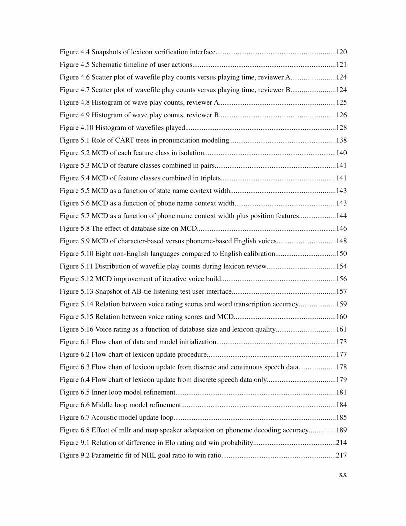
Figure 4.4 Snapshots of lexicon verification interface.................................................................120

Figure 4.5 Schematic timeline of user actions..............................................................................121

Figure 4.6 Scatter plot of wavefile play counts versus playing time, reviewer A........................124

Figure 4.7 Scatter plot of wavefile play counts versus playing time, reviewer B........................124

Figure 4.8 Histogram of wave play counts, reviewer A...............................................................125

Figure 4.9 Histogram of wave play counts, reviewer B...............................................................126

Figure 4.10 Histogram of wavefiles played..................................................................................128

Figure 5.1 Role of CART trees in pronunciation modeling..........................................................138

Figure 5.2 MCD of each feature class in isolation........................................................................140

Figure 5.3 MCD of feature classes combined in pairs..................................................................141

Figure 5.4 MCD of feature classes combined in triplets..............................................................141

Figure 5.5 MCD as a function of state name context width.........................................................143

Figure 5.6 MCD as a function of phone name context width.......................................................143

Figure 5.7 MCD as a function of phone name context width plus position features....................144

Figure 5.8 The effect of database size on MCD............................................................................146

Figure 5.9 MCD of character-based versus phoneme-based English voices................................148

Figure 5.10 Eight non-English languages compared to English calibration.................................150

Figure 5.11 Distribution of wavefile play counts during lexicon review.....................................154

Figure 5.12 MCD improvement of iterative voice build..............................................................156

Figure 5.13 Snapshot of AB-tie listening test user interface........................................................157

Figure 5.14 Relation between voice rating scores and word transcription accuracy....................159

Figure 5.15 Relation between voice rating scores and MCD.......................................................160

Figure 5.16 Voice rating as a function of database size and lexicon quality................................161

Figure 6.1 Flow chart of data and model initialization.................................................................173

Figure 6.2 Flow chart of lexicon update procedure......................................................................177

Figure 6.3 Flow chart of lexicon update from discrete and continuous speech data....................178

Figure 6.4 Flow chart of lexicon update from discrete speech data only.....................................179

Figure 6.5 Inner loop model refinement.......................................................................................181

Figure 6.6 Middle loop model refinement....................................................................................184

Figure 6.7 Acoustic model update loop........................................................................................185

Figure 6.8 Effect of mllr and map speaker adaptation on phoneme decoding accuracy..............189

Figure 9.1 Relation of difference in Elo rating and win probability.............................................214

Figure 9.2 Parametric fit of NHL goal ratio to win ratio..............................................................217

xx

Figure 9.3 Probability distribution function between two Gaussian players................................219

Figure 9.4 Ternary result adjudication between two Gaussian players.........................................220

Figure 9.5 Cumulative density functions of logistics and Gaussian models................................222

Figure 9.6 Difference between two cumulative models...............................................................222

Figure 9.7 Dependence of model log likelihood on number of sample points.............................226

Figure 9.8 Five density functions as a function of (k,n)...............................................................226

Figure 9.9 Maximum likelihood versus minimum error likelihood curves..................................226

Figure 9.10 Interpretation of unbiased estimator as a MAP estimation........................................230

Figure 9.11 Effect of weighting the data with various priors.......................................................231

Figure 9.12 Plot of two priors in rating domain............................................................................233

Figure 9.13 Modification of win probability logistics curve with three priors.............................234

Figure 9.14 Iteration of gammas from equal probability initialization.........................................241

Figure 9.15 Convergence of gammas from a variety of initialization points...............................242

xxi

xxii

1 Introduction

The thesis investigates with what can be done to dramatically reduce the effort required to build

text to speech voices for new languages. In this thesis a language is considered “new” if there are

no existing and acceptable synthetic voices in the target language. For a voice to be acceptable it

must be of sufficient quality and have the desired dialect. Dialect increases the demand for new

voices. While new languages often have small speaker populations, this is not necessarily true.

New languages also tend to be those for which there is a paucity of digital linguistic resources. A

lack of recorded speech, pronunciation lexicons, morphological parsers and so forth increases the

technological difficulty of building new voices because these resources need to be developed.

Such development has heretofore required the involvement of both language experts (linguists)

and speech technology experts. This thesis solves basic impediments, thereby reducing the level

of expertise required to bootstrap synthetic voices.

Specifically, we focus on removing two challenging barriers. First, that of having to explicitly

define a phoneme set during the voice building procedure. And second, that of creating a

pronunciation lexicon. We address the first by automatically inferring phoneme-like units from

two sources: speech collected from the user and a character-based transcript of the recording. The

inferred units are used as the basis for a pronunciation lexicon. Entries in the lexicon are inferred

from a combination of acoustic information and grapheme-to-phoneme rules, and are verified

through user feedback. Consequently, pronunciations can be defined without requiring a language

expert to manipulate phoneme sequences, word by word. Achieving these goals simplifies the

task of voice building sufficient to bring it within reach of people who are not speech technology

specialists. In other words, of making text-to-speech construction accessible to a much broader

audience.

1

The eventual, intended users of this technology are people who want to build a synthesizer in

their own voice, or in the voice of an acquaintance. The user might be a software developer, but

not necessarily. The assumption is that the voice developer is comfortable using desktop software,

either in a traditional GUI application in the form of a browser-based interface, and that they can

understand English at a functional level. A second assumption is that they are literate in the target

language – i.e. that when faced with a word they can speak it and say whether the synthesizer

pronounces it correctly or incorrectly. The user also must be comfortable listening to synthetic

voices. It is helpful if the user can transcribe synthesized test utterances for evaluation.

We call the process of building a synthetic voice in the absence of language-specific prior

knowledge and data “TTS from Zero.” A team of dedicated specialists working on a new

language are operating “from zero” as well. Effectively, the ambition of this thesis is to design

some of that human sophistication into software.

The idea of development from zero may be contrasted with two alternatives. First is voice

transformation. Voice transformation adapts an existing synthesizer of voice V1 in language L1 to

be similar to voice V2, also in L1. Typically it the spectral parameters of the voice are mapped

from V1 to V2 using a comparatively small amount of speech (e.g. 50 utterances, [138]), though

models of F0 and duration can also be transformed. Voice transformation isn't considered TTS

construction for a new language, since the method assumes an existing synthesizer in the same

language. However, the process can amortize the initial investment. Secondly, cross-lingual voice

transformation adapts an existing synthesizer of voice V1 in language L1 to voice V2 in a different

(though preferably similar) language L2. Same-language voice transformation has been heavily

investigated in the past ten years and has evolved into reasonably mature technology [108].

Cross-language voice transformation is a new area of research [166]. Both approaches leverage

off of an existing annotated speech corpus, which serves as a body of prior knowledge. A corpus

of speech supporting multi-lingual voice transformation can be designed as a core of several (i.e.

dozens) of large single-speaker databases, surrounded by many (i.e. thousands) of smaller

“satellite” databases. A voice for a satellite speaker is generated by transforming one of the core

voices. Viewed from this perspective, TTS from Zero substantially reduces the difficulty and

expense of assembling the core.

This chapter continues with a more detailed look at the context and motivation for this work,

noting the distribution of language with fewer than 10 million speakers. From there we define

more precisely the target audience, outlining our working assumptions (section 1.2 ). These lead

to a list of design goals (sections 1.3 ) and our thesis statement (section 1.4 ).

2

1.1 Motivation and context

The dominant economic trend of the past decades has been the expansion of international trade

and commerce to include countries considered a part of or emerging from the Third World. The

rate of growth has been especially rapid in China and India [60], with for example India reporting

an 8.9% growth in GDP for the second quarter of 2006 [76]. In the case of India, the origins of

that country's growth can be traced to specific domestic policy enacted in 1991 [45].

The normal pattern is for economic activity to grow first in large city cores, from there

extending to smaller cities, then finally to rural areas. The desire to hasten this progress,

particularly of information technologies, is exemplified by the Simputer project [80]; as stated in

their mission statement: “the key to bridging the digital divide is to have shared devices that

permit truly simple and natural user interfaces based on sight, touch and audio. It has a special

role in the third world because it ensures that illiteracy is no longer a barrier to handling a

computer.”

Recognizing the need and opportunity, research into speech-based information systems for

non-technical and/or illiterate users is being conducted by a collaboration between Carnegie

Mellon University and Aga Khan University (Karachi, Pakistan), as part of the HealthLine

project.

HealthLine investigates the use of spoken language interfaces for community health workers

across Pakistan. By utilizing state-of-the-art speech recognition, speech synthesis, language

understanding, natural language generation, and dialog management technology, HealthLine

aims to create and pilot a user-friendly, speech-based, telephone-accessible system that

enables the access of relevant health information by a wide spectrum of health workers. [81]

The spread of digital technologies to emerging markets brings with it the opportunity for speech

technology to extend to previously unreached parts of the globe. In areas with large populations

of non-literate people, the case for text-to-speech capability is especially compelling, more so due

to the dominance of the cell phone as the new computing platform of choice [159]. Text to speech

can help bridge the gap between these users and information-based services.

The ability to develop state-of-the-art speech technologies, however, depends to two crucial

ingredients: people that are expert in the various language technologies, and people fluent in the

target language. Locating and acquiring both is difficult; experts, naturally, are in short supply.

Solving this predicament is the motivation behind Carnegie Mellon's SPICE [151].

3

The project SPICE aims to bridge the gap between technology and language expertise by

developing tools that support naive users in building speech processing components in their

language without the need for understanding the underlying technology. Knowledge of the

language in question which is important for the development of speech processing

technologies, is solicited automatically from the user. [139] (p. 91)

SPICE – an acronym for Speech Processing Interactive Creation and Evaluation toolkit – aims

to capture in a software system much of the knowledge of speech technologies experts, while

making it accessible to non-expert users though a web-based interface. It is a toolkit that a) guides

the user in the system creation process while sparing them of the inherent complexities, and b)

solicits information about the target language that would normally be asked by the human

experts. The current focus is on rapid creation of automatic speech recognition and text-to-speech

synthesis components, including the supporting tasks of collecting text, collecting speech,

building n-gram language models, and assembling lexicons. The work of this thesis overlaps with

the SPICE project, concentrating on text-to-speech (TTS) and lexicon creation.

The SPICE toolkit aims to allow a native, literate speaker of any language to create automatic

speech recognition (ASR) for their language and TTS in their own voice. The target does not have

to be among the world's major languages, or have a writing system based on the Roman alphabet.

In a classroom setting, early users of the SPICE have successfully created systems for English,

German, Hindi, Thai, Bulgarian, and Konkani [140].

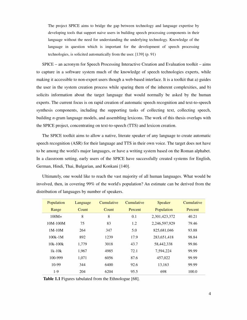
Ultimately, one would like to reach the vast majority of all human languages. What would be

involved, then, in covering 99% of the world's population? An estimate can be derived from the

distribution of languages by number of speakers.

Population

Range

Language

Count

Cumulative

Count

Cumulative

Percent

Speaker

Population

Cumulative

Percent

100M+ 8 8 0.1 2,301,423,372 40.21

10M-100M 75 83 1.2 2,246,597,929 79.46

1M-10M 264 347 5.0 825,681,046 93.88

100k-1M 892 1239 17.9 283,651,418 98.84

10k-100k 1,779 3018 43.7 58,442,338 99.86

1k-10k 1,967 4985 72.1 7,594,224 99.99

100-999 1,071 6056 87.6 457,022 99.99

10-99 344 6400 92.6 13,163 99.99

1-9 204 6204 95.5 698 100.0

Table 1.1 Figures tabulated from the Ethnologue [68].

4

One estimate has that about 1500 of the 6200 languages listed in the Ethnologue (i.e. those with

more than 50,000 speakers) combine to cover 99% of the world population. Relative to this, text-

to-speech is undefined for languages without a writing system. Some of these 1500 languages

will not have a well-accepted writing system and so lie outside the reach of SPICE, while a

number of languages with fewer than 50k speakers do have written systems. (Cornish, a Celtic

language with a writing system, is estimated to have around 3500 speakers.) The web resource

Omniglot [125] lists approximately 700 languages with writing systems and it is safe to

conjecture that this is an underestimate. One thousand, therefore, is a fair figure for the number of

potential languages, and, being a big round number, a nice motivational target.

1.2 Application and assumptions

The goal of this thesis is to enable non-experts to easily build speech synthesis systems for new

languages, in their own voice. Satisfying this goal includes the practical aspect of building

software to support this task, which in turn depends on solving multiple underlying problems of

science and engineering. The underlying problems are substantial, for it amounts to incorporating

into a body of software much of the skill and expertise of a human expert. Most of the sub-steps

required in building voices are well-documented, and are supported with software tools. Notably

this includes the widely distributed free synthesizer Festival [69] and the corresponding voice

construction toolkit Festvox [70]. Nevertheless, Black reminds us that building “very high-

quality speech synthesis is still very much an art, and a set of instructions alone is insufficient”

[139] (pp. 208-9).

Several factors make the process an “art” that demands the skills of an expert. These include:

fundamental decisions about the phoneme set of a language, pronunciation dictionary

development, language-specific text processing, speech corpus collection and labeling, the type

of voice to build (i.e. form of acoustic modeling) – plus understanding of the interaction among

all the components, constraints of speed and memory during training and runtime, and a sense of

where defects are likely to emerge. On top of this is the considerable effort required to evaluate

and fine-tune the synthetic voice, a task made substantially more difficult if it is for a new

language. Because of these difficulties, success in building high quality voices almost invariably

requires the attention of an expert [26][27][28][29].

It is often preferable for a single speech-technology expert to perform the entire voice building

procedure. Given that most people are fluent in only one, or just a handful of languages, the

developer of a text-to-speech voice faces a difficult barrier. Either the technology expert must

5

learn a substantial amount of the language in question, or work in tandem with a suitably

bilingual native speaker. Ideally, the native speaker would not only possess explicit knowledge of

their language, but also be familiar with the needs of speech technology. Usually, it is very

difficult to find such a person.

By “non-expert”1 we take that to mean someone with no advanced training in linguistics or

speech technology, and with limited experience in software development. To distinguish between

expert and non-expert we apply, as a litmus test, the following question. If the answer to “What is

the phoneme set of your language?” results in “Well, that's a complicated question – but here is a

useful starting point for one dialect” then we have found an expert. If the question elicits a

puzzled look then we are dealing with a non-expert.

What is expected of a non-expert and how do we compensate? Since the person is a native

speaker we assume that they are a) literate in their language, b) motivated to create a synthetic

voice, and c) possess sufficient fluency in English to use our software interface. This last

requirement is unfortunate, but presently unavoidable. For our purposes we assume that they can

provide feedback on the quality of speech synthesis. Feedback may involve answering questions

or providing information.

1. Question: is this synthesized word understandable and correct?

2. Question: of these pair of synthesized words, which sounds better?

3. Information: please pronounce this sentence (record user's speech).

4. Information: please transcribe this sentence (from synthesized speech).

In short, we expect that the user is fluent in the target language, and that they are moderately

literate to the point of knowing their character set and basic vocabulary. Notably missing are any

requirements that the user knows what a phoneme is and can define a phoneme set.

1.2.1 Technical limitations

To keep the work of this thesis tractable, certain limitations apply to the target language. First,

that a single writing system is consistently used for the language, or at least that the text collected

is from a consistent standard. Some languages without a long written tradition have competing

writings systems for the same mutually understandable spoken language, including differences in

the computer encoding of digital documents. These issues present real engineering problems, but

1 Sometimes called naïve users, though we avoid use of this term.

6

are outside our scope.

Second, we are not addressing complicated problems of front-end text processing, such as the

notoriously difficult handling of numbers or dates. The text transcripts are constrained to “normal

words.” Third, we assume that the language provides straightforward word segmentation through

whitespace separation. Languages without word demarcation, such as Burmese, present the

additional challenge of automatic word segmentation, an unsolved problem. In addition we

assume that standard ASCII punctuation can be removed without harm.2

We also shy away from tonal languages, since our learning algorithms rely purely on spectral

and duration information, not pitch. If tone is fully marked in the writing system this is less of a

problem, but if it is unmarked then that aspect cannot be properly learned. Agglutinative and

highly inflectional languages are not out of bounds, but a greater practical challenge due to the

combinational growth of word forms.

With these limitations in mind, it should be noted that we are nonetheless building general

purpose synthesizers. Limited domain synthesis can be achieved with relatively limited means,

since they are often phrase-based and employ word substitution, and thus detailed modeling at the

sub-word level is not necessary [20]. All voices in this work are made using the CLUSTERGEN

build tools [24], a framework for building statistical parametric synthesizers [25].

1.3 Design objectives

Adopting a system-guided approach with feedback is the crux of making the voice development

process, but we also want the software to be rewarding to use. We assert that the construction of a

synthetic voice is rewarding if the following conditions hold. That the user: receives early results

(it is gratifying), is able to continually improve the voice incrementally (it is motivating), has a

good chance of succeeding despite making mistakes (it is forgiving), and is in the end able to

achieve a high level of quality (it is satisfying). These positive experiences may be considered as

design objectives. Together, we put forth four major software design objectives. While primarily

intended for non-experts, we do not want to exclude the value that an expert can provide. An

expert will want access to all the software components and data models, and to be able to

diagnose and correct them. The third design goal (that of keeping phonemes hidden) is the critical

element in opening the process to non-experts.

2 Punctuation can change the style of delivery such as emphasis and prosody, but is generally non-

phonemic. A few exceptions can be argued for words such as “bus's” → /b uh s ih z/ in which the

appostrophe is mapped to the phoneme /ih/.

7

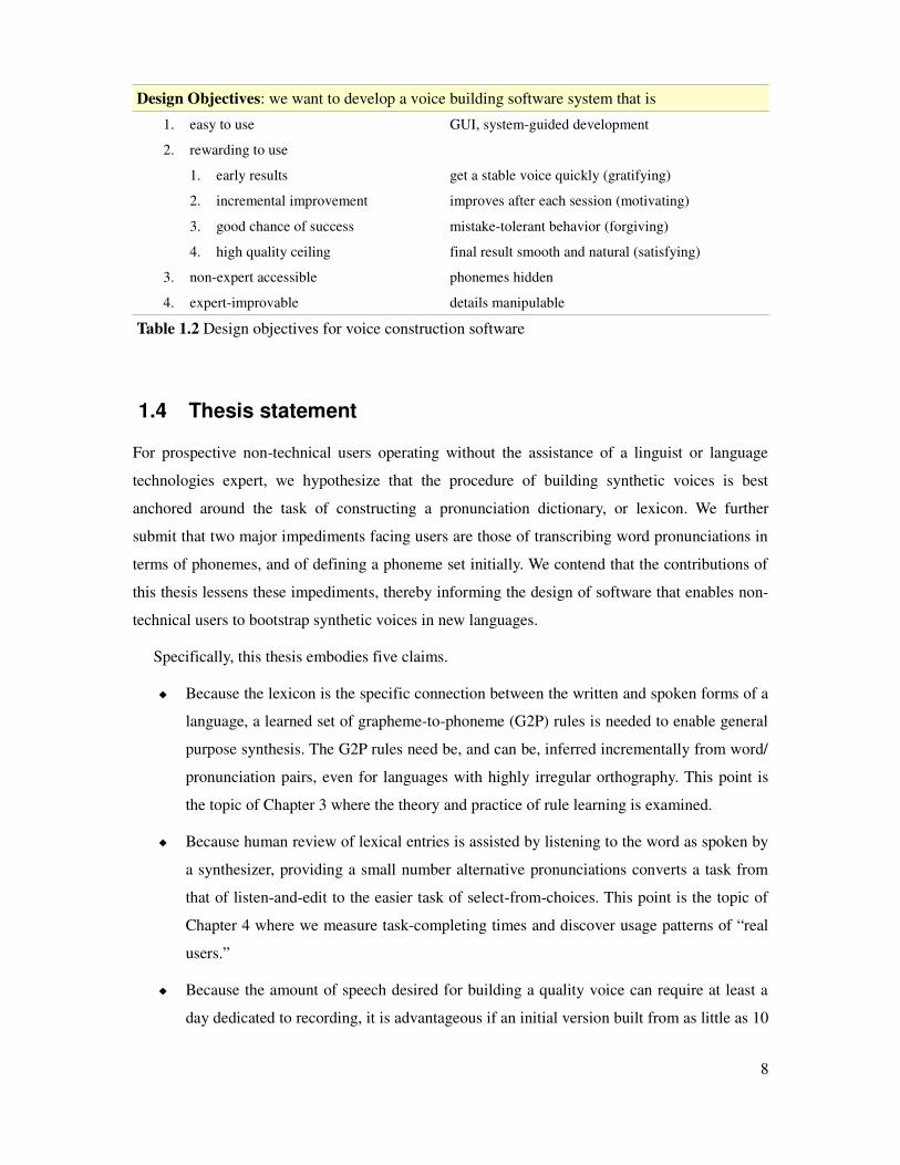
Design Objectives: we want to develop a voice building software system that is

1. easy to use GUI, system-guided development

2. rewarding to use

1. early results get a stable voice quickly (gratifying)

2. incremental improvement improves after each session (motivating)

3. good chance of success mistake-tolerant behavior (forgiving)

4. high quality ceiling final result smooth and natural (satisfying)

3. non-expert accessible phonemes hidden

4. expert-improvable details manipulable

Table 1.2 Design objectives for voice construction software

1.4 Thesis statement

For prospective non-technical users operating without the assistance of a linguist or language

technologies expert, we hypothesize that the procedure of building synthetic voices is best

anchored around the task of constructing a pronunciation dictionary, or lexicon. We further

submit that two major impediments facing users are those of transcribing word pronunciations in

terms of phonemes, and of defining a phoneme set initially. We contend that the contributions of

this thesis lessens these impediments, thereby informing the design of software that enables non-

technical users to bootstrap synthetic voices in new languages.

Specifically, this thesis embodies five claims.

Because the lexicon is the specific connection between the written and spoken forms of a

language, a learned set of grapheme-to-phoneme (G2P) rules is needed to enable general

purpose synthesis. The G2P rules need be, and can be, inferred incrementally from word/

pronunciation pairs, even for languages with highly irregular orthography. This point is

the topic of Chapter 3 where the theory and practice of rule learning is examined.

Because human review of lexical entries is assisted by listening to the word as spoken by

a synthesizer, providing a small number alternative pronunciations converts a task from

that of listen-and-edit to the easier task of select-from-choices. This point is the topic of

Chapter 4 where we measure task-completing times and discover usage patterns of “real

users.”

Because the amount of speech desired for building a quality voice can require at least a

day dedicated to recording, it is advantageous if an initial version built from as little as 10

8

minutes of speech can provide useful feedback and suffice as a starting point. Success is

possible because language-independent features (as used during the build procedure for

all languages) account for the majority of modeling accuracy. This point is the topic

Chapter 5 where users build several non-English voices from little data.

Because a voice can be bootstrapped from little data, it can be successfully improved by

the user through an iterative cycle of recording, lexicon construction, and synthesis

evaluation. Voice quality can be evaluated through sentence transcription, through paired-

comparison listening tests, and estimated by the objective measure of mel cepstral

distortion (MCD). To assess progress, the relationship between MCD and the amount of

speech collected is established, as is the relationship between MCD and paired-

comparison listening tests. This point is the topic of the second half of Chapter 5 where

consideration is made of the time spent on each part of the build cycle (recording, lexical

work, evaluation).

Because a phoneme set provides a potent mediating layer between orthography and

phonetics, and because phoneme sets are difficult for humans to define, an empirical

phoneset can be initialized from graphemes and refined through merge and split

operations. In relieving the user of this burden one transforms the software's role to that

of jointly learning the phoneset, lexicon, and G2P rules. This joint problem can be

constrained by having the user provide acoustic samples of the lexicon by recording

words in isolation. Through resynthesis of the samples we can determine each word's

pronunciation as spoken. This point is the topic of Chapter 6, where a speech recognition

decoder and speech synthesizer are used in tandem to infer pronunciations directly from

acoustic evidence.

Combined, these investigations provide the information necessary to engineer a software system

capable of achieving “TTS from Zero.”

1.5 Organization of thesis

Chapter 2 begins with a description of the synthesis pipeline – the series of steps (in a

prototypical system) for the conversion of textual input to speech output. This leads to the role of

phonemes as linguistic units and the foundational role that a phoneset plays in a speech

synthesizer. While the International Phonetic Association delineates a broad range of phonetic

elements and provides a handbook on the usage of the IPA alphabet [86][85], there is no

handbook where one may conveniently look up the phoneme inventory of any given language.

9

We illustrate this point with languages of the Indian subcontinent. The lack of such a universal

reference indicates the difficultly of the task, a point we take up when discussion the design

freedom of phoneme sets.

Following in Chapter 2, we discuss four approaches to defining a phone set and building

pronunciation dictionaries for uncovered languages. We discuss the strengths and weaknesses of

each and argue that two of these are both novel and feasible. One of these approaches uses

graphemes as seeds for the initial phoneset, while the other makes use of a multi-lingual ASR

decoder to suggest a seed set. The first is more applicable when the grapheme-to-phoneme

relationship is relatively straightforward, while the second is likely to be successful when the new

language is well covered by the database. Chapter 2 outlines the component solutions required in

a grapheme-based approach and reviews some of the more relevant literature.

Chapter 3 concentrates on the role of grapheme-to-phoneme rules in a speech synthesizer. A

G2P system encapsulates in an algorithmic framework the relation between the spelling and

pronunciation of words in a lexicon. A G2P rule set has the ability to provide predictions for

unseen words (those not in the lexicon) – a crucial capability needed by a synthesizer. It is also

useful for the training of acoustic models in both ASR and TTS. In certain formulations, G2P

rules can predict multiple pronunciations for a given word. This capability is instrumental in this

work. We present present some common formulations for rule systems, explaining our selection,

and developing the algorithm to suit our task of learning pronunciations with the assistance of a

human verifier. A theme that runs throughout this thesis is “how can an interactive system make

best use of the user's knowledge and time?”. An aspect of this question is the issue of word

selection strategies – of having the system present questions to the user in a manner that is

optimal. Some languages have a straightforward relation between graphemes and phonemes

(where this issue matters less), while in others it is complex. This range of complexity is

demonstrated by offline test on a small suite of popular languages for which large pronunciation

dictionaries are available.

Chapter 4 documents lexicon development conducted by native speakers in a realistic setting.

Specifically, for Iraqi Arabic in the context of an existing speech-to-speech translation system.

This includes the task of employing human reviewers to verify words in an existing dictionary,

and of adding new words. This effort uses the G2P tools developed in Chapter 3. The emphasis of

this chapter lies in measuring the usage pattern of native speaking non-technologist users, and in

particular of measuring the time required to perform careful verification. Careful verification is

assisted by providing synthesized versions of pronunciation variants, which the reviewers listen

10

to and judge.

Chapter 5 progresses from lexicon maintenance in and existing system to synthesizer

development in new languages. We begin by analyzing the degree to which synthesizer training

depends on language-dependent features that only a human expert can provide. Comprehensive

offline experiments in English suggest that the dependency is not strong, clearing the way for

non-experts to successfully build voices in new languages. In a series of small-scale projects in

eight non-English languages, users built synthesizers out of small amounts of data. At the outset,

users were asked to a phoneme set for their language, and to record a single speaker database of

at least 200 sentence-length prompts. The lexicon and G2P rules are developed incrementally

using the web-based interface of the SPICE tools. The synthesizer is built in a single batch

processing stage. After building a synthesizer the user evaluated the voice quality by means of

informal assessment and through transcription tests of heldout sentences.

A desirable goal is to permit users to incrementally build voices under the guidance of a voice

building system. Incremental construction means that the voice is built not merely once, at the

end of all data preparation, but multiple times during the learning process. The process is guided

if the system can suggest a course of action that will improve the synthesizer the most, for

example in recording more speech to improve coverage, or to fix pronunciation errors. To support

this goal a means of automatically measuring voice quality is required. Throughout this thesis we

adopt the objective distortion measure of mean mel cepstral distortion (MCD). To assess the

viability of MCD we perform systematic calibration experiments against English voices. Within

the framework, as established by the calibration experiments, we can estimate the quality of non-

English voices. However, using the objective measure of MCD can only provide an overall

estimate of voice quality. More precise feedback is provided through transcription and A-B

listening preference tests. We find that as a voice is incrementally improved, there is a strong

correlation between objective and subjective evaluations. With guided incremental voice building

a real prospect, we examine the time required of users to perform the three tasks of: recording

speech, constructing a pronunciation lexicon, and performing listening tests. Measurements of

where users spend their time provides valuable information for future improvements.

Chapter 6 attacks the problem of automatically inferring a phoneset and lexicon form acoustic

data. We develop an approach to phoneset and lexicon inference in which the role of an ASR

decoder is to suggest pronunciation hypotheses, and the role of the synthesizer is to evaluate them

in an integrated analysis-synthesis loop. Again, MCD is the metric employed to select among the

hypotheses. The essential idea is to build a lexicon in which the synthesizer selects entries that

11

minimize TTS distortion. The phoneset can seeded from graphemes – thereby creating the initial

ASR/TTS model pair – and expanded iterative through split/merge operations. Similar to Chapter

5, a human user can be in the loop verifying the lexicon and incrementally recording additional

speech to improve the synthetic voice.

The final chapter, 7, summarizes what has been accomplished and concludes with possible

extensions and future developments.

12

2 Background

Since we aim to make the development of voices for uncovered languages easier and more

automated, it is helpful to review the processing stages of speech synthesis and relate that to voice

building. Following this overview, this chapter focuses on the role played by phonemes and

phonesets in TTS. This is followed by a selection of related work.

2.1 The synthesis pipeline

Using the Festival system as an exemplar, Table 2.1 lists its twelve main processing stages. These

are the conversion of the input text to attribute-bearing tokens, the conversion of tokens to words,

of words to strings of phonemes, followed by the addition of prosodic information, and finally

conversion to a waveform.

In a high-quality voice, each of these stages requires the attention of an expert, either to create

the necessary supporting models, or to program by hand those components that cannot be easily

automated. Notably, the conversion into words of numbers and other non-standard tokens is so

complex and varied across languages that human specification is unavoidable [153]. In SPICE,

consequently, text normalization is confined to relatively simple operations of case conversion

and punctuation removal, though invoking heavier computational machinery is possible [154].

Also for the sake of simplicity, waveform generation is based on the CLUSTERGEN method that

is a standard part of Festival [24]. Despite exhibiting the “buzziness” of vocoded speech, for our

application it is the best choice because it known to be stable when built from small amounts of

speech, down to ten minutes or less [104]. The spectral and prosody models can be built

automatically provided that a lexicon and phoneme set is available.

13

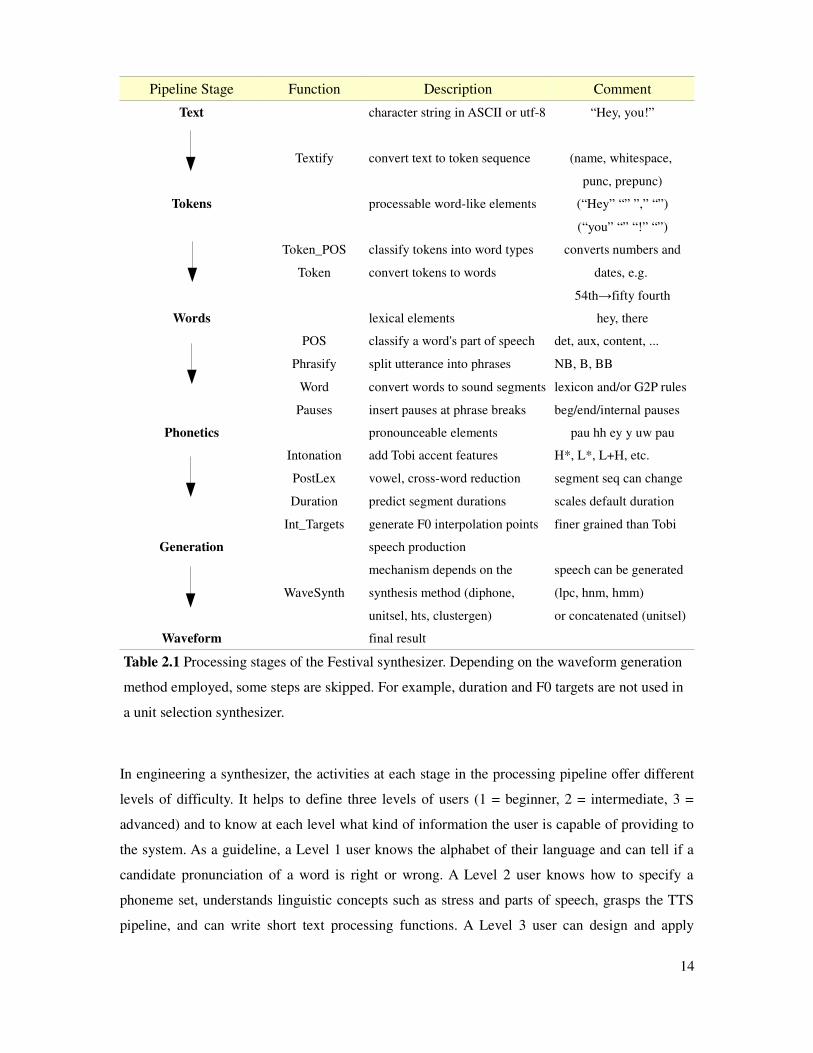
Pipeline Stage Function Description Comment

Text character string in ASCII or utf-8 “Hey, you!”

Textify convert text to token sequence (name, whitespace,

punc, prepunc)

Tokens processable word-like elements (“Hey” “” ”,” “”)

(“you” “” “!” “”)

Token_POS

Token

classify tokens into word types

convert tokens to words

converts numbers and

dates, e.g.

54th→fifty fourth

Words lexical elements hey, there

POS

Phrasify

Word

Pauses

classify a word's part of speech

split utterance into phrases

convert words to sound segments

insert pauses at phrase breaks

det, aux, content, ...

NB, B, BB

lexicon and/or G2P rules

beg/end/internal pauses

Phonetics pronounceable elements pau hh ey y uw pau

Intonation

PostLex

Duration

Int_Targets

add Tobi accent features

vowel, cross-word reduction

predict segment durations

generate F0 interpolation points

H*, L*, L+H, etc.

segment seq can change

scales default duration

finer grained than Tobi

Generation speech production

WaveSynth

mechanism depends on the

synthesis method (diphone,

unitsel, hts, clustergen)

speech can be generated

(lpc, hnm, hmm)

or concatenated (unitsel)

Waveform final result

Table 2.1 Processing stages of the Festival synthesizer. Depending on the waveform generation

method employed, some steps are skipped. For example, duration and F0 targets are not used in

a unit selection synthesizer.

In engineering a synthesizer, the activities at each stage in the processing pipeline offer different

levels of difficulty. It helps to define three levels of users (1 = beginner, 2 = intermediate, 3 =

advanced) and to know at each level what kind of information the user is capable of providing to

the system. As a guideline, a Level 1 user knows the alphabet of their language and can tell if a

candidate pronunciation of a word is right or wrong. A Level 2 user knows how to specify a

phoneme set, understands linguistic concepts such as stress and parts of speech, grasps the TTS

pipeline, and can write short text processing functions. A Level 3 user can design and apply

14

machine learning techniques to train phonetic models. An expert also grasps the consequences of

design choices – phoneset choice, unit clustering, labeling procedure, speech parameterization,

etc. – and can feed corrective information back into the build process.

Pipeline Stage Function Level 1 Level 2 Level 3

Text Textify defines the characterset includingwhitespace andpunctuation

specify foreignlanguage charactersthat may appear

converts text touniform encoding(Unicode)

Tokens Token_POS ––– regular expressions toidentify numbers, dates

construct a token_posCART tree

Token normalization ofcommon numbers

code to perform simpletext normalization

converter of English-level complexity

Words POS ––– limited homographPOS disambiguation

train POS CART onlarge tagged corpus

Phrasify ––– use punctuation forphrasing levels

train ngram phrasingmodel

Word select pronuns fromwavefile examples

define phoneme set,add lexical entries

train G2P CART treeon full lexicon

Pauses ––– map break type topause durations

train pause lengthsfrom phrase structure

Phonetics Intonation ––– ––– train intonation andaccent-target cart tree

PostLex ––– ––– write reduction andco-articulation rules

Duration ––– provide average phonedurations

train duration carttree from labeled data

Int_Targets ––– rules: add accent tostressed vowels intcontent words

train F0 prosodymodels on normalizepitch data

Generation WaveSynth ––– tune synthesis controlparameters

write synthesis DSPcode

Table 2.2 Activities of each stage by level of user sophistication. Highlighted is the area of

concentration of this thesis.

In summary, there are three critical areas where user input is necessary in addition to recording

speech. These are 1) providing sufficiently large examples of text in the target language, from

which the character set and word list my be extracted. 2) Defining the phoneme set of the

language's sound system. And 3) providing pronunciations for words in the lexicon. The large

amount of effort required to bootstrap a pronunciation dictionary from nothing is well known

[50]. More error prone and technically difficult, even, is the challenge of defining a phoneme set.

15

2.2 The role and challenge of phonemes

This section elaborates on the central role that phonemes play in a synthesizer, and the inherent

difficulty in defining a good phoneset, particularly as faced by a non-expert. The terms phone and

phoneme are often used interchangeably (as is common in the literature), yet they are distinct

concepts and we want to be precise in our terminology. In fact the concept of a phoneme – its

exact nature and even validity – is a matter of long-standing dispute within the linguistics

community. While we won't wade into the debate here, we will state our definitions and venture

our perspective that phonemes constitute the “atoms of speech.”

Because spoken language is both a tool of cognition and mechanism of communication, the

study of speech spans the disciplines of articulatory phonetics (production), acoustic phonetics

(transmission), auditory phonetics (perception), linguistics (comprehension) and neuro-linguistics

(encoding) – plus the application of information theory and learning theory. The phoneme is

central in all of these, and thus expresses different aspects depending on the scientific point of

view.

2.2.1 Definition of terms

Phonemes are the minimal meaning-contrastive units of a language's sound system. In this

definition meaning-contrastive establishes that it is a concept of perception and comprehension.

According to some schools of thought, phonemes are said to be “linguistic abstractions,” but in

itself this is an insufficient description, for it does not specify an abstraction of what. The qualifier

minimal clarifies that we are referring to the smallest coherent elements of speech that distinguish

meaning. By analogy, letters are the minimal meaning-contrastive units of a language's writing

system. Strictly speaking, phonemes are defined within, and confined to, a single language only.

Similar sounding units from different languages are not the same phoneme – because they are a

not a part of the same sound system; if two sounds systems are mutually incomprehensible – i.e.

they are from different languages – there can be no basis for meaning contrast.

The minimal pair test provides the essential scrutiny. A phoneme is identified when two

different words differ in only one minimal sound. The words “pat” and “bat” isolate the p/b

distinction for example. Conversely, “paternal” and “parenting” do not isolate a minimal unit.

This highlights an idea implicit in the definition of phoneme, but for the sake of economy is not

stated. When speaking of minimal units, it is understood that it is continuous segments of speech

that are being perceived; they do not interleave in time.

16

The phoneme set of a language is the full set of that language's inventory of phonemes. Words

are auditory, visual, or tactile symbols that represent concepts3. Spoken words are composed from

predominantly unique sequences of phonemes (with the qualifier “predominantly” permitting

confusable word pairs such as “there” and “their”) whose interpretation is unambiguous in

context.

Phones are clusters of similar sounding speech units that are usually but not necessarily

phoneme-like. Phones are a concept of acoustic phonetics and are looser in that they are not

restricted to being meaning-contrastive. For example, the stop and release components of plosives

may be treated as separate phones, as can the allophonic distinction between dark and light /l/. A

phoneset is a set of phones defined for some purpose, often ASR or TTS. A phoneset may be

multilingual.

Among many writers the term phone refers to a particular acoustic realization of a phoneme –

a “surface realization” – such that it may be recorded and played back (see for example [82] or

[93]). We avoid this usage for it imports the premise that phonemes are empty linguistic

abstractions devoid of particular content. In our usage a phone is a broad generalization covering

an unlimited number of instances, equally as much as the concept of phoneme does. Nevertheless,

it is still useful to refer to particular acoustic realizations and, when the context is clear, phone has

proved handy for this purpose. As is the convention, forward slashes indicate that the object of

discussion is a phoneme – /p/ – while square brackets denote a phone – [p].4

An allophone is a perceptually relevant variant of a phoneme, where the variation is often

predictable by surrounding context. Similarly, phones can be subdivided into perceptually

relevant variants. A triphone is phone variant where the context is exactly specified by the

preceding and following phone. In speech synthesis it is common to deal with phone subtypes,

where the specification is more general (and often automatically generated using a CART tree

learner). In the nomenclature of the SPHINX speech recognition system [148][149], the phone

subtypes are senones [150]. When phones are divided in time they are temporal sub-phones,

though due to the prominence of HMM-based acoustic modeling in speech technology it is typical

to simply refer instead to states, with the understanding of what is meant.

3 Visual is needed to include written and sign language (such as ASL), while tactile covers Braille. The

remaining human senses (smell and taste) are too diffuse to support a discrete alphabet that is necessary

for conceptual communication.

4 Confusing matters further, forward slashes are commonly used for broad phonetic transcription of

speech, while square brackets are reserved for narrow phonetic transcription, e.g. /p/ versus [ph].

17

Though not common terminology, one may speak of gestural phonemes and gestural phones.

This shifts the focus from acoustic phonetics to articulatory phonetics, i.e. to speech production.

From this perspective a phoneme is considered an articulatory target, or target trajectory that is

meaning-contrastive when perceived. Fortunately for human communication, small changes in

articulation results in distinct changes in sound. Critically, the relation between the two realms is

largely, if not entirely, one-to-one. This correspondence permits a classification scheme that is

universal across all spoken languages, and is the basis for the International Phonetic Alphabet.

2.2.2 The International Phonetic Alphabet (IPA)

The International Phonetic Alphabet (IPA) is a product of the International Phonetic Association

(also IPA) [86]. Its purpose is to catalog and organize the sounds of the world's languages on the

basis of articulatory phonetic principles, to collect and provide corresponding acoustic examples

from the world's languages, to provide a universal standard notation, and to offer guidelines on

the transcription of speech. In the words of John Wells, the contemporary caretaker of the

alphabet, “the symbols are basically intended to symbolize phonemes (sound classes)” – thereby

expressing the point of view of acoustic phonetics. However, in discussing the nature of broad

versus narrow transcription, he then adds that “in speaking of allophones, I am thinking of

articulatory allophones” [173]. Regardless of which way a phoneme is conceived, the units are

organized according to principles of articulatory, not acoustic, phonetics. This is apparent in the

main IPA charts, reproduced below in Table 2.3. Specifically: consonants are organized by

manner and place of articulation (vertical and horizontal axes), plus voicing. Vowels are

organized by height and backness, plus rounding.

By definition, a phoneme in the IPA organization is categorized by how it is produced, not

how it sounds or how it fits into the sound system of a language. This organizing principle is what

makes the IPA an articulatory phonetic alphabet, not an alphabet of phonemes – even though the

basic intention is to catalog phonemes. Since a phoneme is defined only within a language there

can be no such thing as an interlingual (international) phonemic alphabet. But this distinction is

almost splitting hairs. Because humans share the same vocal apparatus, this universality permits

similarity-based groupings across languages. Given this ambition, the great variety of human

languages forces the inclusion of a vast array of features; this is apparent in the diacritics chart.

To illustrate: a /t/ may be: labialized, palatalized, velarized, pharengalized, alveolar, dental,

apical, laminal, and linguolabial. A /t/ in most dialects of English is understood to be alveolar,

while that in Hindi is dental. Such details are typically not retained in a broad transcription,

18

though they can be attended to and annotated. Since differences of production exist on continuum

of greater and finer distinctions, the decision of when to group sounds together as essentially the

same, and when to keep them separate, is optional and can be adapted to the application at hand.

Table 2.3 The IPA consonant, vowel and diacritic charts (revised to 2005).

2.2.3 The GlobalPhone corpus and phone set

The GlobalPhone corpus is a multilingual set of read speech databases collected for research and

development in ASR, developed at Karlsruhe university in Germany [136]. It is suitable for large

vocabulary multilingual continuous speech recognition and has been used to construct language-

adaptive and (to a significant extent) language-independent systems. From the mid 90s to 2002 a

total of 15 languages were collected: Arabic, Chinese-Mandarin, Chinese-Shanghai, Croatian,

Czech, French, German, Japanese, Korean, Brazilian Portuguese, Russian, Spanish, Swedish,

Tamil, and Turkish.

19

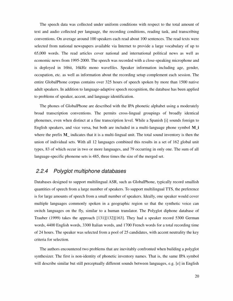
The speech data was collected under uniform conditions with respect to the total amount of

text and audio collected per language, the recording conditions, reading task, and transcribing

conventions. On average around 100 speakers each read about 100 sentences. The read texts were

selected from national newspapers available via Internet to provide a large vocabulary of up to

65,000 words. The read articles cover national and international political news as well as

economic news from 1995-2000. The speech was recorded with a close-speaking microphone and

is deployed in 16bit, 16kHz mono wavefiles. Speaker information including age, gender,

occupation, etc. as well as information about the recording setup complement each session. The

entire GlobalPhone corpus contains over 325 hours of speech spoken by more than 1500 native

adult speakers. In addition to language-adaptive speech recognition, the database has been applied

to problems of speaker, accent, and language identification.

The phones of GlobalPhone are described with the IPA phonetic alphabet using a moderately

broad transcription conventions. The permits cross-lingual groupings of broadly identical

phonemes, even when distinct at a fine transcription level. While a Spanish [i] sounds foreign to

English speakers, and vice versa, but both are included in a multi-language phone symbol M_i

where the prefix M_ indicates that it is a multi-lingual unit. The total sound inventory is then the

union of individual sets. With all 12 languages combined this results in a set of 162 global unit

types, 83 of which occur in two or more languages, and 79 occurring in only one. The sum of all

language-specific phoneme sets is 485, three times the size of the merged set.

2.2.4 Polyglot multiphone databases

Databases designed to support multilingual ASR, such as GlobalPhone, typically record smallish

quantities of speech from a large number of speakers. To support multilingual TTS, the preference

is for large amounts of speech from a small number of speakers. Ideally, one speaker would cover

multiple languages commonly spoken in a geographic region so that the synthetic voice can

switch languages on the fly, similar to a human translator. The Polyglot diphone database of

Trauber (1999) takes the approach [131][132][163]. They had a speaker record 5300 German

words, 4400 English words, 3300 Italian words, and 1700 French words for a total recording time

of 24 hours. The speaker was selected from a pool of 25 candidates, with accent neutrality the key

criteria for selection.

The authors encountered two problems that are inevitably confronted when building a polyglot

synthesizer. The first is non-identity of phonetic inventory names. That is, the same IPA symbol

will describe similar but still perceptually different sounds between languages, e.g. [e] in English

20

is perceptually different from [e] in German, and exchanging one for the other results in speech

that sounds “off” to a native listener. Using sound classes that are shared between languages (to

save effort) is acceptable in some cases, but not all. The second problem is that of transcription

consistency. Pronunciations dictionaries differ in their conventions in describing sounds. Some

are purely phonemic while others are phonetic, with still others a mixture of the two. Inconsistent

conventions poses difficulty in labeling diphones, and in expanding the pronunciation dictionary

(among other problems), and makes it harder to build a uniform sounding synthesizer.

language words diphones

German 5300 2500

English 4400 2200

Italian 3300 1400

French 1700 1600

Table 2.4 Composition of Polyglot diphone database.

2.2.5 The paucity of defined phoneme sets

The most straightforward answer to “what is a language's phoneme set?” is to look it up in an

encyclopedia of linguistics. This imposes an up-front burden – for someone has to hunt down

reference works, struggle with incomplete data as well as conflicting or archaic notation, make it

consistent, and enter it in useful format. While burdensome, this is a way to provide support of

major languages, as was done for GlobalPhone [136]. It is then possible to incorporate such

information into a software system and present it in a menu offering. When this groundwork is in

place, the user merely has to find their language name from the available list.

The weakness of this approach is one of coverage. Even if the language is found, there is a

substantial chance that it doesn't represent the speaker's own dialect. More severely, the majority

of languages that we are trying to reach will not be listed at all. An instructive case can be made

with regard to the languages of India, where even the number of languages spoken is unclear. The

SIL Ethnologue lists 415 living languages for India [68]. Wikipedia cites an “official figure of

'mother tongues' spoken in India of 1,683, of which an estimated 850 are in daily use [175]. The

government of India has declared 22 languages as officially recognized for government

communication at the federal level, in addition to English. These cover the largest fraction of the

population, and are listed in Table 2.5 below, with approximate population figures. Also included

are some other significant languages of India, bringing this compilation to a total of 32.

21

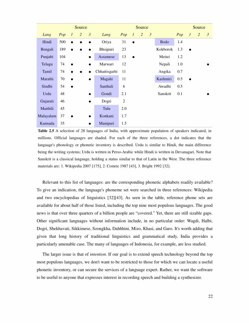
Source Source Source

Lang Pop 1 2 3 Lang Pop 1 2 3 Pop 1 2 3

Hindi 500 Oriya 31 Bodo 1.4

Bengali 189 Bhojpuri 23 Kokborok 1.3

Punjabi 104 Assamese 13 Meitei 1.2

Telugu 74 Marwari 12 Nepali 1.0

Tamil 74 Chhattisgarhi 11 Angika 0.7

Marathi 70 Magahi 11 Kashmiri 0.5

Sindhi 54 Santhali 6 Awadhi 0.5

Urdu 48 Gondi 2.1 Sanskrit 0.1

Gujarati 46 Dogri 2

Maithili 45 Tulu 2.0

Malayalam 37 Konkani 1.7

Kannada 35 Manipuri 1.5

Table 2.5 A selection of 28 languages of India, with approximate population of speakers indicated, in

millions. Official languages are shaded. For each of the three references, a dot indicates that the

language's phonology or phonetic inventory is described. Urdu is similar to Hindi, the main difference

being the writing systems; Urdu is written in Perso-Arabic while Hindi is written in Devanagari. Note that

Sanskrit is a classical language, holding a status similar to that of Latin in the West. The three reference

materials are: 1. Wikipedia 2007 [175], 2. Comrie 1987 [43], 3. Bright 1992 [32].

Relevant to this list of languages: are the corresponding phonetic alphabets readily available?

To give an indication, the language's phoneme set were searched in three references: Wikipedia

and two encyclopedias of linguistics [32][43]. As seen in the table, reference phone sets are

available for about half of those listed, including the top nine most populous languages. The good

news is that over three quarters of a billion people are “covered.” Yet, there are still sizable gaps.

Other significant languages without information include, in no particular order: Wagdi, Halbi,

Dogri, Shekhavati, Sikkimese, Szongkha, Dahhhini, Mizo, Khasi, and Garo. It's worth adding that

given that long history of traditional linguistics and grammatical study, India provides a

particularly amenable case. The many of languages of Indonesia, for example, are less studied.

The larger issue is that of intention. If our goal is to extend speech technology beyond the top

most populous languages, we don't want to be restricted to those for which we can locate a useful

phonetic inventory, or can secure the services of a language expert. Rather, we want the software

to be useful to anyone that expresses interest in recording speech and building a synthesizer.

22

2.2.6 The design freedom of phoneme sets

Thought it is possible in some cases to locate phoneme sets in reference books, this does not

imply that the task of defining a phoneme set is easy. It is not. Phoneticians are known to spend

years debating the phoneme set of a particular language before, if ever, reaching a consensus.

Fortunately for our purposes, a consensus is not required. When dealing with speech

technologies, engineering considerations take precedence. This provides considerable freedom of

design beyond the inherent difficulty of specifying a phoneme set.

To buttress this claim, consider the following observations.

There is no universally accepted phoneme set for English. This can be seen by comparing

the many English dictionaries, including traditional hardbound tomes such as Websters

and Colliers, and specialized pronunciation dictionaries such as Jones [92] and Wells

[174]. There is a core of overlap, but considerable variation at the edges.

Strictly, one needs to speak of the phoneme sets of dialects, rather than the language

itself. There are easily dozens of dialects of English across the world [91] that all bleed

into one another. The /x/ of Scottish English, as in the word “loch” for example, will

sometimes appear in a non-Scottish dialect.

Since the boundaries are not sharply delimited, it is not even clear how many dialects

there are of a language. In the authoritative survey of Labov [114], North America has

seven major dialects (West, South, Midland, North-Central, Mid-Atlantic, New York City,

and Canadian) but there are many minor dialects including Pennsylvania Dutch and

Canadian Maritimes.

Languages sometimes borrow phonemes from other languages in order to acquire loan

words. For example the English /w/ has been adopted by German speakers to say the

word “Windows”.

Dialects evolve over time and can drop phonemes as unfashionable. In the mid-20th

century American English lost the aspirated velar approximate /wh/ as used to be

pronounced in the words “whales” (compare “Wales”) and “where” (compare “wear”).

Sometimes allophones are promoted into the phoneme set, even if they are not strictly

speaking meaning-contrastive units. This is a result of continuous speech being spoken

differently from careful speech. In inter-vocalic settings in English the /t/ and /d/ are

frequently reduced to taps (a separate element of the IPA), and /k/ is often realized as a

23

glottal stop. This perspective places greater weight on the distinctiveness of sound and

articulation since there are no examples of minimal pairs.

Similarly, most practical phoneme sets include the short mid-vowel schwa, though it

originates as a reduced form of multiple target vowels. Subtle though uncommon schwa

contrasts such as between “Lennon/linen” argues for two central reduced phonemes.

In rhotic sound systems, the r-coloring of vowels can result in an increase in the phoneme

set. The inclusion of rhoticized vowels is not always uniform. In DARPABET-based

phonesets commonly used for American English ASR and TTS, “heard” is transcribed as

three phonemes – /h er d/ – while “hard” has four: /h aa r d/. The criteria for creating a

dedicated phone is fuzzy and is often done for technical reasons.

Moving from linguistic issues to those of speech technology, a phoneme may be

collapsed into a neighboring category if it is rarely occurring. The Janus recognition

system [72], for example, merges /zh/ with /sh/ or /jh/ on the grounds that there are not

enough examples to reliably train acoustic models for /zh/. The Sphinx recognition

system, in contrast, makes no special effort to prune out under-trained phonemes.

In the DARPABET/ARPABET set, syllabified /l/ /m/ and /n/ are given separate symbols

/el/ /em/ and /en/ to describe words such as the battle, bottom, and button [127] (p. 24).

The Carnegie Mellon University pronunciation dictionary adopted these in it's original

version, but are dropped in more recent editions [42].

In the case of the Sphinx speech recognition system, one can point to the historical

evolution of its phoneme set through three major iterations. Changes included the

elimination of deletable stops consonants, and the high schwa vowel /ix/ [128].

Finally, one can point to the history of English speech synthesizer as proof of design

freedom.

Table 2.6 provides a comparison between various dictionaries covering American English. It

presents the subset of vowels (plus the “dead” consonant /wh/) where there is a difference in

representation. Those not shown are included in all of the dictionaries – i.e. there is agreement on

all of the “core” vowels. Differences arise with respect to short central vowels (schwas),

palletized vowels (present in the Holmes synthesizer), the rare diphthong /oy/, and imported

foreign vowels (included in the traditional Columbia dictionary). Not shown are any variations

due to stress marking.

24

IPA CMU

DICT

Sphinx

ver1

Sphinx

ver2

Janus Timit Pron-

lex

Fest-

dict

Holmes AHD Klatt Examples

\ AX AX AX ax ax ax a \ about

\h axh

| AXR AXR axr butter

û IX IX ix ix debit

øj OY OY OY oy oy oy oi oi boy

u° ux ux dude

ju yu youth

e® air ââ care

i® eer pier

¨® oor fur

Å ¼ pot

Ø öö French bleu

y üü French tu

„ WH where

Table 2.6 Differences in English vowel sets between various dictionaries. CMUDICT and the

two Sphinx versions are from [42], Janus is from [137], Pronlex is from [99], the Festival and

Holmes phonesets are from [69], and AHD is from The American Heritage Dictionary [2], Klatt

is from [84].

2.3 Pronunciation modeling in speech synthesis

It is not an exaggeration to assert that everything a speech synthesizer does is pronunciation

modeling. Since the purpose of the software or hardware is to generate intelligible speech, the

pronunciation of a word in a sentence is, literally, the exact waveform produced. The synthesizer

must traverse the full path from orthography to physical realization, as per Figure 2.1.

Pronunciation modeling in speech technology is often conceived as a dictionary lookup

operation that converts a word to a sequence of phonemes. In the sense that this is where most of

the information lies, this perspective is valid. But full pronunciation modeling progresses through

multiple layers. A useful point of comparison is the five-level labeling typology of Barry and

Fourcin [14]. Their typology is intended to guild phoneticians in the creation of labeled speech

databases for linguistic study.

25

Level Characteristics

phonemic Use of functionally distinctive sounds units of a language as the principle

mediator between the lexicon and sound signal.

broad phonetic Only uses symbols that have phonemic status, but uses the symbol set

indicate a more acoustically accurate description of continuous speech. For

example a tapped /t/ may be transcribed as [d] if there is no /‰/ defined.

narrow phonetic Uses IPA symbol set to differentiate the realized sounds (allophones) with

respect to the base sound. Differentiation is in terms of nasality, rounding,

centrality, length, etc.

acoustic phonetic Uses full complement of IPA symbols to provide a high fidelity symbolic

representation of continuous speech. Includes descriptors such as stop

closure, release burst, and aspiration. The criteria for assigning a label to a

segment of speech is acoustic homogeneity.

physical The physical measurements of speech production. Most typically this is the

acoustic waveform, but may include other tracks such as electroglottalgraph,

electropalatograph, electromagnetic articulograph, nasal airflow, etc.

Table 2.7 Five levels of Barry and Fourcin's labeling typology.

To illustrate, consider a two-word utterance “forget it” that is pronounced casually, as might be

written “fergeddit.” The four symbolic levels could be transcribed like this.

phonemic: /f ao r g eh t ih t/ is the concatenation of careful forms listed in a

pronunciation dictionary.

broad phonetic: [f er g eh d ih t] transcribes the /t/ as a sound more typical of /d/ and

that the first vowel of “forget” is reduced to the more casual /er/.

narrow phonetic: [f er g eh d ih t¬] annotates that the final /t/ is unreleased.

acoustic phonetic: [f er gc g eh dc d ih t¬] splits the stop consonants into closure and

release parts and notes the movement of the word-final /t/ into the following syllable.

From a computational perspective, two or three phonetic levels may be grouped into post-lexical

processing. The transformations may be within-word or cross-word alterations of the phonemic

level. This short utterance is illustrated in Figure 2.1 with broad and narrow phonetic layers

merged. The tree includes syllable structure to show phoneme movement into the word “it.”

26

Figure 2.1 Hierarchy of symbolic pronunciation processing from text to numerics.

The bottom two layers of Figure 2.1 are the lowest levels of symbolic processing. The state level

divides each phone into three subphones, or states. This division is typically hard-coded into the

synthesizer and mimics the 3-state HMM architecture common to ASR. Associated with each

state is a function s that maps the state into a sequence of 5ms frames. The number of frames

per state is predicted by a duration model. The frames themselves are multidimensional vectors of

numbers used to encode spectral features, power, F0, and possibly voicing. Thus the function

s incorporates both spectral and prosodic modeling. At this low level, pronunciation

modeling is the problem of converting text to a low-distortion vector sequence. Figure 2.2 plots

an example of predicting the first cepstral dimension. Beneath the frame level (not shown) is the

waveform generated from the sequence of frames.

27

Γ(s)

G2P

[g][gc]

[f]

[d]

eh2

/t/

forget it

/r//ao//f/ /ih//t//eh//g/

[t]

[t][ih][d][eh][g][er]

forget it

[dc]

eh3

0 1 0 syllable stress

words

orthography

phonetic

post-lexical

phonemic

graphemes

frame

stateeh1

’f’ ’r’’o’ ’e’’g’ ’i’’t’

[er]

’t’

[f] [ih][eh]

Figure 2.2 Pronunciation modeling at the feature generation level. The curves plot 500 frames of

speech, comparing the original and synthesized trajectories for the first cepstral dimension.

2.3.1 Phonemes as a mediating layer

In practice it is not unusual for the lexicon to replace canonical (phonemic) pronunciations with

common variants from the broad phonetic level. For example the entry for “forget” may be in the

more casually (frequently) spoken form of /f er g eh t/. To the extent that this is done, much of the

phonetic processing is moved up into the lexicon and frozen into place. If the phoneset is

identical to the phoneme set then the lexicon is broadly phonetic. If finer distinctions are made

then the lexicon is more narrowly phonetic. For example the TIMIT labeling system defines

syllabic nasal, reduced alveolar stops, and voiced /h/ among others. When this enlarged suite of

symbols is used to compose the pronunciations, the lexicon is narrowly phonetic. Miller assessed

the ability of artificial neural networks to execute post-lexical rules in a speech synthesizer. Time-

delay neural networks converted from the phonemic layer to the narrow phonetic [118].

base allophone base allophone base allophone

/d/ d ‰ d dx /m/ m m§ m em /u/ u ∏ uw

/t/ t t¬ ‰ ? t dx /n/ n n§ n en /û/ û û≤ π ax ix

/h/ h Ó hh hv /l/ l l§ l el

Table 2.8 TIMIT-based allophones used by Miller's post-lexical rules.

28

Frame Number

0 100 200 300 400 500

c1 - first cepstral dim

ension

-1.0

0.0

1.0

2.0

3.0

MCD = original - synthesized

Legend

original

synthesized

The inherent limitation of a phonetic lexicon is that it cannot represent cross-word modifications

due to co-articulation and anticipatory effects. Another downside of a narrow phonetic lexicon is

the difficulty of covering the range of variation and doing so consistently. Given these

considerations the architecture of a speech synthesizer will often simplify the processing levels.

The lexicon will be phonemic or broadly phonetic, while post-lexical processing is pushed down

to the state→frame conversion function. To handle allophonic variation and co-articulation one

then relies on s for the training of x from the acoustic data. This choice reduces the control

available with explicit symbolic processing, but offers the advantages of machine learning – the

capacity to handle larger amounts of data with greater fidelity.

Observe that when machine learning of s is engaged, the phonemic and phonetic symbolic

layers can be discarded entirely. In a grapheme-based synthesizer the transformation passes

directly from graphemes to frames. For languages with uncomplicated grapheme-to-phoneme

sound systems this is a viable first approximation. More complicated languages benefit from

having a mediating symbolic layer. The mediation may be multi-layered employing broad and

narrow symbol sets and post-lexical transformation rules. Or the mediation may be single-layered

involving just phonemes and a lexicon so derived.

The working premise of just about all speech systems is that the architecture benefits from an

intermediate, mediating layer. In this thesis we adopt the view that one can potentially start with

an un-mediated grapheme-based system and progressively learn a mediating layer. The learning

proceeds from a combination of text, acoustic information, and feedback from the human

building the voice.

2.4 Possible solutions

In the following table we organize the range of options for bootstrapping a phoneset and

pronunciation dictionary for an uncovered language. There are four types of approaches to

consider. First, in what may be called the “user defined” or “established method” relies on a

native speaker or technology expert to define a phoneme set and build up a lexicon manually. On

the basis of this information a set of G2P rules are learned and used to extend pronunciation

coverage out-of-vocabulary words. Various non-traditional alternatives do not require the user to

define a phoneme set, and so must be derived through other, i.e. automatic, means.

29

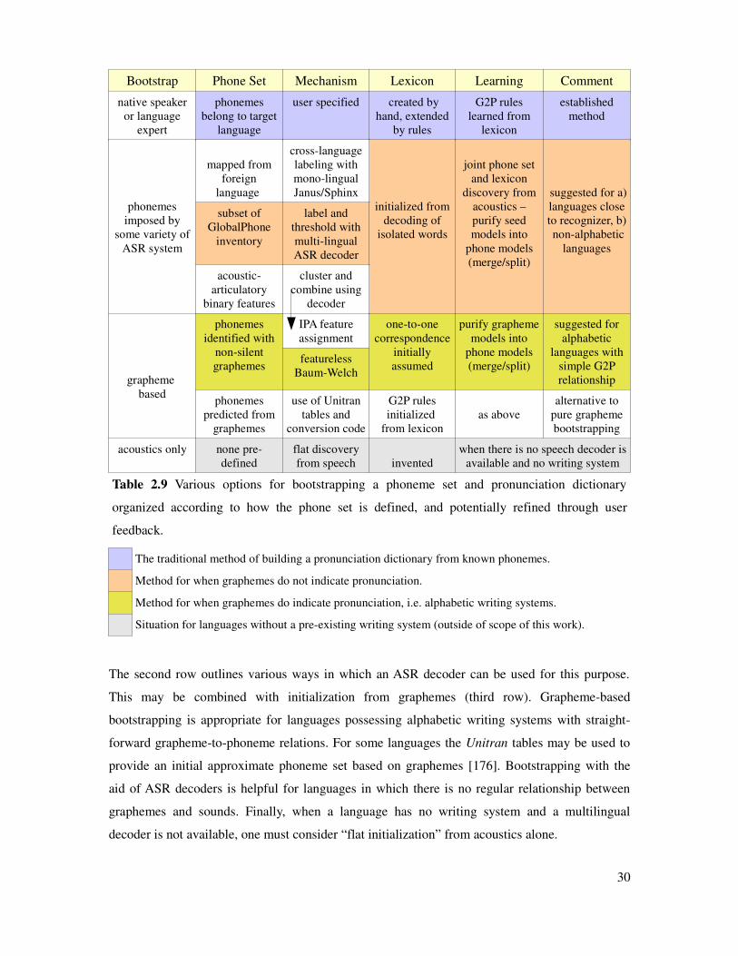
Bootstrap Phone Set Mechanism Lexicon Learning Comment

native speakeror language

expert

phonemesbelong to target

language

user specified created byhand, extended

by rules

G2P ruleslearned from

lexicon

establishedmethod

phonemesimposed by

some variety ofASR system

mapped from

foreignlanguage

cross-languagelabeling withmono-lingualJanus/Sphinx

subset ofGlobalPhone

inventory

label andthreshold withmulti-lingualASR decoder

acoustic-articulatory

binary features

cluster andcombine using

decoder

initialized fromdecoding of

isolated words

joint phone setand lexicon

discovery fromacoustics –purify seedmodels into

phone models(merge/split)

suggested for a)languages closeto recognizer, b) non-alphabetic

languages

grapheme based

phonemesidentified with

non-silentgraphemes

IPA featureassignment

featurelessBaum-Welch

one-to-onecorrespondence

initiallyassumed

purify graphememodels into

phone models(merge/split)

suggested foralphabetic

languages withsimple G2Prelationship

phonemespredicted from

graphemes

use of Unitrantables and

conversion code

G2P rulesinitialized

from lexiconas above

alternative topure graphemebootstrapping

acoustics only none pre-defined

flat discoveryfrom speech invented

when there is no speech decoder isavailable and no writing system

Table 2.9 Various options for bootstrapping a phoneme set and pronunciation dictionary

organized according to how the phone set is defined, and potentially refined through user

feedback.

The traditional method of building a pronunciation dictionary from known phonemes.

Method for when graphemes do not indicate pronunciation.

Method for when graphemes do indicate pronunciation, i.e. alphabetic writing systems.

Situation for languages without a pre-existing writing system (outside of scope of this work).

The second row outlines various ways in which an ASR decoder can be used for this purpose.

This may be combined with initialization from graphemes (third row). Grapheme-based

bootstrapping is appropriate for languages possessing alphabetic writing systems with straight-

forward grapheme-to-phoneme relations. For some languages the Unitran tables may be used to

provide an initial approximate phoneme set based on graphemes [176]. Bootstrapping with the

aid of ASR decoders is helpful for languages in which there is no regular relationship between

graphemes and sounds. Finally, when a language has no writing system and a multilingual

decoder is not available, one must consider “flat initialization” from acoustics alone.

30

2.4.1 Strengths and weaknesses of possible solutions

The above four solutions we refer to as: 1) User Defined (or, the “established method”), 2) ASR

Imposed, 3) Grapheme Based, and 4) Pure Acoustics. They are primarily distinguished according

to how the initial phone set is established, as this has deep consequences for the rest of the

system.

Each of these four approaches has strengths and weaknesses.

1. As discussed earlier, asking the user to define their phoneme set is a difficult task and is a

bottleneck in the entire procedure. However, if the user is an expert in linguistics and

speech technology, this is the most secure route to success.

2. Adopting ASR-imposed phonemes has the obvious precondition of requiring a speech

classification system. This renders the user dependent on the system's breadth of

coverage and accuracy of decoding. The advantage is that it incorporates prior knowledge

of many of the world's language in the form of multilingual acoustic models [155].

3. Grapheme-based initialization is attractive, but since no system of writing is in direct

one-to-one correspondence with pronunciation, this approach is challenged to a degree

that depends on the language. However, it offers the significant advantage of direct

bootstrapping from written transcripts, which are much less costly to acquire than

phonetic transcriptions.

4. In “discovery from pure acoustics,” the objective is to clustering speech into similar

sounding units on the basis of the speech alone, then affiliate these clusters with

phonemes. Little prior knowledge or seeding of the clusters is imposed. This is probably

an under-constrained task.

It is worth mentioning a hybrid approach that combines the first two. In particular, one begins

with the established method of defining a phone set and lexicon by hand, and from that build an

ASR decoder (collecting large amounts of speech in the process). With this in place one can

extend the lexicon by using the decoder to analyze out of vocabulary words. This procedure is

known as “baseform determination” [13]. It is used to either add new words the the lexicon (such

as for surnames), or to add alternate pronunciations to existing words. While potentially useful

once the system is developed, it doesn't solve our problem for it depends on a pre-existing

decoder in the language we are trying to bootstrap. Also, baseform-determination typically

requires many examples of the same word (ten or more) to produce reliable results [115].

31

2.4.2 Applicability of approaches

Because it is best understood and easiest to implement, the first deployment of the SPICE toolkit

adopted the “established method.” Our studies of [140] and [104] reported on the experiences of

technically proficient users. For this category of user, the established method is the surest path to

success. For non-expert users, the grapheme-based approach is ultimately our method of choice.

It is applicable when the writing system is alphabetic in nature. If the grapheme to sound

relationship is uncomplicated, it may be sufficient to adopt the non-silent graphemes as the

phoneme set [21]. In most cases, though, the grapheme to sound relationship is complex enough

to necessitate a stage of refinement, or “untangling of the sounds.”

Despite the simplicity that a grapheme-based approach to synthesis provides, it does introduce

a handicap: graphemes are mere symbols, without any indication of acoustic properties, i.e. the

IPA features of place, manner, voicing etc. This is a problem because the voice building

procedure works more successfully when it has acoustic features at its disposal. One way to

compensate is to inject the missing IPA features by employing a multilingual acoustic-articulatory

recognizer, e.g. of Stüker [156]. However, as demonstrated in Chapter 5, the handicap is not

large. Even when phonemes attribute-free, voices can successfully be built.

For languages in which there is little or no correspondence between graphemes and sounds (in

particular Chinese), extracting a phone set from the graphemes cannot be accomplished. One

option is to forgo the acquisition of a phone set entirely and resort to what is essentially a word-

based synthesizer. Or, one can attempt to discover a phone set through other means, i.e.

application of a multilingual speech recognizer [170] run in phoneme-decoding mode. This is

indicated in Table 2.9 as “label and threshold with multi-lingual ASR decoder”.

It's worth noting that applying the GlobalPhone recognizer for the purpose of automatically

extracting a phone set can be applied to all languages [155], and this can establish a valuable

point of comparison. From the perspective of acoustic modeling, the benefit is that it embeds

prior knowledge of approximately 15 diverse languages. The disadvantage is that it is unclear

how well it can extrapolate beyond its base of known languages. In this regard the drawbacks are

the same as that of single-language decoding, except that problems of under-coverage are not

encountered as often, or as severely. Investigation of these issues are outside of the scope of this

thesis, but are worth raising as potential future work.

Decoding from pure acoustics is the course of last resort, when there is no writing system or

written material available. Research in this direction includes [38] and [89].

32

2.5 Related work

Rapid development of language technologies in an ongoing area of research in both machine

translation [110] and speech recognition [66][138]. An organization with goals similar to that of

the SPICE project is the Local Language Speech Technology Initiative [113][165]. The LLSTI has

developed a handful of speech synthesizer for African languages and reported on the issues of

porting TTS to new languages [75][143][164]. Also involved in the development of synthesizers

for new languages is the Meraka Institute of South Africa [117]. In this thesis, our investigations

into G2P rule inference and bootstrapping of pronunciation dictionaries overlaps most closely

with the work of Davel and Barnard [46][47][48][49][50][51][52][53][54][55][56][57][58][59].

They have released a lexicon building software tool called DictionaryMaker based on their

Default & Refine algorithm [63]. To aid the lexicon development process, DictionaryMaker

synthesizes the predicted pronunciation by concatenating wavefiles of isolated phonemes of the

target language. Maskey does not prepare synthesized examples of pronunciations, but instead

developed a confidence measure that is applied to the symbolic prediction. Words with high a

confidence level are skipped over, thereby saving the user the effort of validating probably-

correct words [116]. His work with G2P rule learning builds on that of Pagel [18][19] and

Chotimongkol [40].

Font Llitjós investigated the possibility of bypassing the phoneme layer entirely in building

unit selection synthesizers for Catillian and Columbian dialects of Spanish [21]. Spanish has a

highly regular G2P relationship but is not one-to-one. The experiments established the voice

building procedure could separate the variant pronunciations of 'c' (/ch, k, s, th/) and of 'g' (/g, j/)

with an overall word pronunciation error rate between 6.4% and 9.2%.

The alternative to boostrapping a system in a new language is to perform cross-language

adaptation, or transfer, of existing models. Most commonly this is accomplished through a

phoneme-to-phoneme mapping. Efforts in cross-language adaptation for ASR include Kienappel

[98], Sooful [147], and Schultz [135]. Phoneme transformation has been used in unit selection

TTS [12][35] and statistical parametric TTS [22][23][108]. Tomokiyo addresses the problem of

foreign accent intrusion [161]. The phoneme mapping between languages is typically based on

the designer's experience and performed by hand. Regarding phoneme mapping, Le proposes

some particular automatic methods based on heuristic phonetic similarity [112].

Except for the grapheme-based voice of Llitjós, all of the systems mentioned rely on a pre-

existing or a human-constructed lexicon. Inferring lexical entries from the available acoustics is

33

commonly known as baseform determination. Baseform determination is usually performed with

the assistance of an existing ASR decoder [13][115]. The purpose of the discovered pronunciation

forms is to extend the lexicon of the ASR system to cover previously out-of-vocabulary words, or

to add alternate pronunciations that reduce overall word error rates. Observing that the baseform

suggestions of phonetic decoding can be erratic, Anumanchipalli used the decoder to evaluate a

list of provided pronunciation alternatives [4]. In his approach, G2P rules trained on a large

existing dictionary plays the role of suggesting pronunciations, and of providing probabilities for

each suggestion [section 3.1.6.1]. These probabilities are further weighted with phone transition

probabilities [section 3.1.7] and with likelihoods provided from Viterbi forced alignment. In the

typology of Table 2.7 these are broad phonetic additions to the lexicon. In contrast, Tajchman

used ASR decoding to generate narrow phonetic transcriptions for the purpose of learning

probabilistic phonological rules [158]. Closer to our purpose, Prahallad altered the architecture of

a speech decoder at the level of phone topology [126]. The topologies were either a) linear 5-state

sequential with no skip states, b) fully connected 5-state networks, or c) linear 5-state sequential

with fully connecting forward jumps. The states are all context-independent, single Gaussian

mixtures. For each topology, the pronunciation of a word is the transition through its respective

network. Experiments showed that model b) had the best average log likelihood on the training

data, followed by model c). This suggests that topologies with a higher degree of freedom can

better model detailed pronunciation, particularly in the case of conversational speech.

The combined problem of joint lexicon and phoneset determination was first addressed by

Bacchiani [7][8][9][10]. Through repeated split operations Bacchiani grew the phone inventory

from 124 context-independent states up to 1519 tied triphone states (senones). The final

dictionary entries are defined in terms of these 1519 senones – and is thus very fine-grained and

not a traditional lexicon. Singh and Raj have also developed techniques for join phoneset and

lexicon discovery [122][123][146]. In one experiment they initialized a context-independent ASR

system with a 50-item phoneset, performed six merge operations to reduce the phoneset to 44

phones, then expanded it back up to 50 [144]. (Experiments were based on the 50-phone version

CMUDICT that was commonly in use at the time.) The mergers contained the pairs /ae, eh/, /axr,

r/, /dd, td/, /m, n/ and the triple /ax, ix, ih/. In a second experiment they initialized ASR system

with the 26 letters of English, then performed two batches of eight phone splits, i.e. the phoneset

size jumped from 26 to 34 to 42 (but not, mysteriously, to 50) [145]. The Resource Management

task was used to compare the seven automatically derived systems to a reference benchmark.

Comparisons were made for both context-independent and context-dependent models.

34

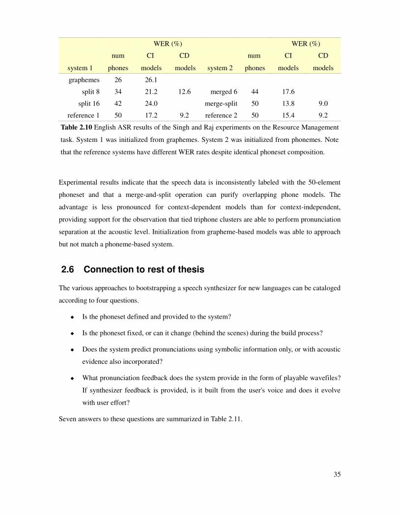
WER (%) WER (%)

system 1

num

phones

CI

models

CD

models system 2

num

phones

CI

models

CD

models

graphemes 26 26.1

split 8 34 21.2 12.6 merged 6 44 17.6

split 16 42 24.0 merge-split 50 13.8 9.0

reference 1 50 17.2 9.2 reference 2 50 15.4 9.2

Table 2.10 English ASR results of the Singh and Raj experiments on the Resource Management

task. System 1 was initialized from graphemes. System 2 was initialized from phonemes. Note

that the reference systems have different WER rates despite identical phoneset composition.

Experimental results indicate that the speech data is inconsistently labeled with the 50-element

phoneset and that a merge-and-split operation can purify overlapping phone models. The

advantage is less pronounced for context-dependent models than for context-independent,

providing support for the observation that tied triphone clusters are able to perform pronunciation

separation at the acoustic level. Initialization from grapheme-based models was able to approach

but not match a phoneme-based system.

2.6 Connection to rest of thesis

The various approaches to bootstrapping a speech synthesizer for new languages can be cataloged

according to four questions.

Is the phoneset defined and provided to the system?

Is the phoneset fixed, or can it change (behind the scenes) during the build process?

Does the system predict pronunciations using symbolic information only, or with acoustic

evidence also incorporated?

What pronunciation feedback does the system provide in the form of playable wavefiles?

If synthesizer feedback is provided, is it built from the user's voice and does it evolve

with user effort?

Seven answers to these questions are summarized in Table 2.11.

35

method

phoneset

provided

phoneset

fixed

system

predicts with

synthesizer

feedback investigated

traditional yes yes none none ––

Davel yes yes G2P rules phone concat. ––

method 1 yes yes G2P rules prebuilt synth. Chp 4

method 2 yes yes G2P rules IPA synth. Chp 5

method 3 yes yes G2P + acoustics built voice Chp 5

method 4 yes no G2P + acoustics built voice Chp 6

method 5 no no G2P + acoustics build voice Chp 6

Table 2.11 Comparison of seven approaches for lexicon and synthesizer development.

36

3 G2P Rules

The role of Grapheme-to-Phoneme rules is to convert text into a sequence of phonemes, or

phones, more generally. Typically text is consumed on a word-by-word basis, but even languages

written without word segmentation can be processed. In text to speech applications the original

value offered by G2P rules was the capability for reducing a large pronunciation dictionary into a

more compact form that can fit into small memory capacities. Even when memory size is not a

constraint, G2P rules serve the indispensable purpose of predicting the pronunciations of out of

vocabulary words. In languages with highly regular spelling, such as Portuguese and Spanish, the

rules may simply be hard coded into software. In more complex languages the rules may be

written by hand or discovered using a machine learning algorithm of some choosing. Languages

with complex phonology,5 such as English and German, have benefited greatly from

automatically learned rules because hand-written rules are difficult to develop and maintain, and

are prone to oversights. This is certainly true for English, as will be shown in section 3.1.1 where

we examine an example of a hand-written rule system.

Many different rule formalisms and prediction algorithms have been applied to the problem of

grapheme to phoneme conversion (otherwise known as letter-to-sound or LTS rules). The next

section covers some of the common approaches, including the two predominant methods of

CART trees and linear rewrite rule chains with expanding context triggers. Of these, the

formalism adopted for our research is that of rewrite rule chains.

While we speak of grapheme-to-phoneme rules, they are a more general tool than that. They

are symbol conversion rules – a function that maps from one discrete alphabet to another. For

example, the rules can be trained to operate in the reverse direction, to convert from phonemes to

5 Pronunciation variations due to gender agreement is treated upstream by the text normalization module.

In French, “1 fille” (1 girl) becomes “une fille” not “un fille” (compare 1 boy: “un garçon”) [64].

37

letters. The tool may also be applied to problems of phonology, i.e. of converting phonemes to

allophonic variants (e.g. the tap in “butter”) or accounting for co-articulation (e.g. the assimilated

word-final /k/ in “bank card”). Depending on the architecture there may be two layers in

converting text: first graphemes to phonemes, then phonemes to (allo)phones. The two layers of

transformation may be combined into one compound function. Alternatively, only conversion to

the first layer may be performed, without attempting to explicitly generate symbols at the detailed

phonetic level. The work of this thesis uses a single layer transformation, relying on the acoustic

model of Figure 2.1 to complete the conversion.

After a general discussion of G2P rules, section 3.2 describes our algorithm in more detail.

Section 3.3 presents offline experiments on numerous languages. Then section 3.4 investigates

the question of word ordering. Can the order in which words are presented to the system

accelerate the learning process? What is the shortest sequence of words that will result in the

same rules as that built from the entire set? This question is particularly relevant when the

“system” is a human user entering pronunciations online.

3.1 Some approaches to G2P conversion

The most common approach to G2P conversion is little more than a formalism of what children

learn in school: that a letter, say 'p', usually indicates a particular sound: /p/, except when the

following letter modifies the sound. For example if the following letter is an 'h', then you group it

as 'ph' and the sound is /f/. Except that won't work for words such as “uphill” so the 'ph' rule is

qualified to apply to word-initial p's. But the words “symphony” and “batphone” are fine, thus the

question becomes: is there a syllable break between the 'p' and 'h'? And so forth.

In the formalism promoted by Chomsky and Halle [39], G2P transformations are controlled by

symbolic rewrite rules conditioned on left and right context. For this small example the rule is:

1. 'p' → f / #_h generally /lc _ rc

2. 'p' → p / _

The rightmost part is the rule context, and is of the form lc_rc, where left context lc and right

context rc are regular expressions. The underscore separates them and serves as a placeholder for

the central letter 'p'. The hash mark indicates a word boundary. To convert the input grapheme the

first, more specific rule is checked first. If the left and right contexts both match, it is applied.

Otherwise the second rule is checked. A blank on either side of the underscore means that

38

anything matches, so if this rule is reached it is guaranteed to apply; it provides the default

pronunciation. Davel uses the terminology “Default and Refine” for rewrite rules arranged in this

fashion [49], and this is the formalism that we adopted for our work. Because the rules are

arranged in a linear chain, other acceptable terms are “rule chain” and “decision list.”

Most G2P approaches are some kind of rule network. A few others are substantially different.

Stem and affix rules. This decomposes words into morphological components. If one has

pronunciations of “up” and “hill” and “able” then one can pronounce “uphill” and

“uphillable” by concatenation (uphillable adj. capable of going uphill).

Rule chains with multi-character input and output. This is similar to above except that the

input can be sequences of letters, such as “ph” and “pp”. This is exemplified below with

respect to the hand-written Wasser rules for American English.

Finite state transducers. This used the mechanism of finite state automata for conversion.

Rule chains and decision trees have an equivalent DFA form and in practice are often

“compiled down” to automata [73][152].

CART or decision trees. This is another common choice for G2P representation. They

differ from rule chains primarily regarding architecture. Instead of rules being organized

into linear lists, they are arranged into binary branching tree structures. Rule chains are

the degenerate form of trees. Decision trees are discussed below in section 3.1.3 where

they are compared to rule chains [18][88].

Hidden Markov models. An HMM can be trained in which phonemes are the hidden

symbols and letters are the observations. Then, the decoding problem is the find the most

probable sequence of phone state given the observation sequence [160].

Statistical machine translation. The heavy machinery of statistical MT can be brought to

bear on translating from language L1 (graphemes) to language L2 (phonemes). This is

overkill, really, since the problem does not have issues of word rearrangement, phrase

restructuring, and divergent morphology. Yet one can train and apply, for example, the

IBM translation models “1” through “3” [33].

Latent semantic analogy (principal components analysis) [16][17]. Pronunciation by

latent semantic analogy begins by performing singular value decomposition on a corpus

of word strings, (subdivided into identical length subsets). This permits dimensional

reduction to a small number of principal components, i.e. n = 2. Each training word

39

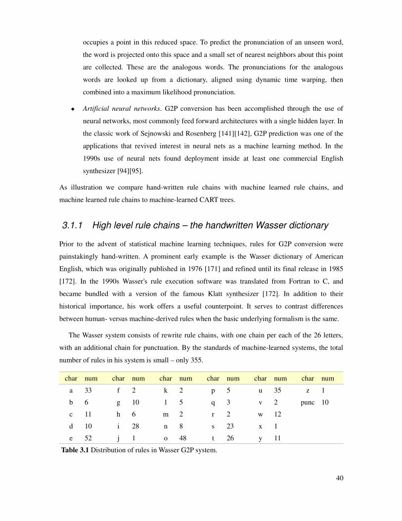
occupies a point in this reduced space. To predict the pronunciation of an unseen word,

the word is projected onto this space and a small set of nearest neighbors about this point

are collected. These are the analogous words. The pronunciations for the analogous

words are looked up from a dictionary, aligned using dynamic time warping, then

combined into a maximum likelihood pronunciation.

Artificial neural networks. G2P conversion has been accomplished through the use of

neural networks, most commonly feed forward architectures with a single hidden layer. In

the classic work of Sejnowski and Rosenberg [141][142], G2P prediction was one of the

applications that revived interest in neural nets as a machine learning method. In the

1990s use of neural nets found deployment inside at least one commercial English

synthesizer [94][95].

As illustration we compare hand-written rule chains with machine learned rule chains, and

machine learned rule chains to machine-learned CART trees.

3.1.1 High level rule chains – the handwritten Wasser dictionary

Prior to the advent of statistical machine learning techniques, rules for G2P conversion were

painstakingly hand-written. A prominent early example is the Wasser dictionary of American

English, which was originally published in 1976 [171] and refined until its final release in 1985

[172]. In the 1990s Wasser's rule execution software was translated from Fortran to C, and

became bundled with a version of the famous Klatt synthesizer [172]. In addition to their

historical importance, his work offers a useful counterpoint. It serves to contrast differences

between human- versus machine-derived rules when the basic underlying formalism is the same.

The Wasser system consists of rewrite rule chains, with one chain per each of the 26 letters,

with an additional chain for punctuation. By the standards of machine-learned systems, the total

number of rules in his system is small – only 355.

char num char num char num char num char num char num

a 33 f 2 k 2 p 5 u 35 z 1

b 6 g 10 l 5 q 3 v 2 punc 10

c 11 h 6 m 2 r 2 w 12

d 10 i 28 n 8 s 23 x 1

e 52 j 1 o 48 t 26 y 11

Table 3.1 Distribution of rules in Wasser G2P system.

40

The rule chain for 'p' is compact enough to serve as illustration. It has five rules.

id. match output left right

p1 ph → /f/ any any

p2 peop → /p iy p/ any any

p3 pow → /p aw/ any any

p4 put → /p uh t/ any #

p5 p → /p/ any any

Table 3.2 Wasser rules for the letter 'p'.

The first thing to notice is that the match part is not restricted to being a single character, but can

be an unlimited substring. As well, the output can be single or multiple symbols. The rule

application algorithm thus operates on matching substring prefixes. For example if the word is

“philip” and the cursor points to the word beginning, “ph” matches due to rule 1. After producing

the output symbols the cursor skips the 'h' and moves to the third character 'i'. The consequence is

that two letter collocations are treated as a unit. The rules for 'h' do not contain an entry that says

if the previous character is a 'p' then produce the epsilon symbol (i.e. zero-duration silence).

Notice also that the middle three rules include vowel output. Presumably, 'peop' → /p iy p/ was

included to specifically handle the word “people.”

The ability to represent substrings is one mechanism by which the rule set is kept compact.

Another is the use of predefined general-context symbols. The contexts are regular expressions.

ID predefined special context translation

C1 v+ one or more vowel letters

C2 c* zero or more consonants letters

C3 c one consonant letter

C4 [bd v g j l m n r w z] voiced consonant letters

C5 _[e er es ed ely ing] right context suffix

C6 [e i y] front vowel letters

Table 3.3 Predefined contexts in Wasser G2P system.

The special contexts consolidate what would require multiple rules if the match parts could be

defined only in single letters. For example, context C5 is the “suffix rule.” It allows the single

rule 'a' → /ey/ _C3C5 to cover the words bare, barer, bares, barely, baring (in contrast to“bar”).

To continue the illustrating example of the letter 'p' we introduce here a small corpus of eight

words: people, pepper, philip, phony, pseudo, pterodactyl, chapter, stephen.

41

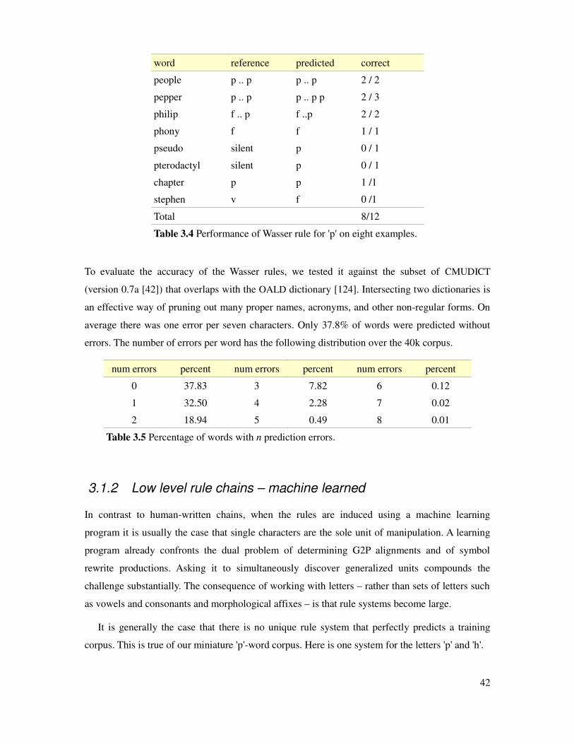
word reference predicted correct

people p .. p p .. p 2 / 2

pepper p .. p p .. p p 2 / 3

philip f .. p f ..p 2 / 2

phony f f 1 / 1

pseudo silent p 0 / 1

pterodactyl silent p 0 / 1

chapter p p 1 /1

stephen v f 0 /1

Total 8/12

Table 3.4 Performance of Wasser rule for 'p' on eight examples.

To evaluate the accuracy of the Wasser rules, we tested it against the subset of CMUDICT

(version 0.7a [42]) that overlaps with the OALD dictionary [124]. Intersecting two dictionaries is

an effective way of pruning out many proper names, acronyms, and other non-regular forms. On

average there was one error per seven characters. Only 37.8% of words were predicted without

errors. The number of errors per word has the following distribution over the 40k corpus.

num errors percent num errors percent num errors percent

0 37.83 3 7.82 6 0.12

1 32.50 4 2.28 7 0.02

2 18.94 5 0.49 8 0.01

Table 3.5 Percentage of words with n prediction errors.

3.1.2 Low level rule chains – machine learned

In contrast to human-written chains, when the rules are induced using a machine learning

program it is usually the case that single characters are the sole unit of manipulation. A learning

program already confronts the dual problem of determining G2P alignments and of symbol

rewrite productions. Asking it to simultaneously discover generalized units compounds the

challenge substantially. The consequence of working with letters – rather than sets of letters such

as vowels and consonants and morphological affixes – is that rule systems become large.

It is generally the case that there is no unique rule system that perfectly predicts a training

corpus. This is true of our miniature 'p'-word corpus. Here is one system for the letters 'p' and 'h'.

42

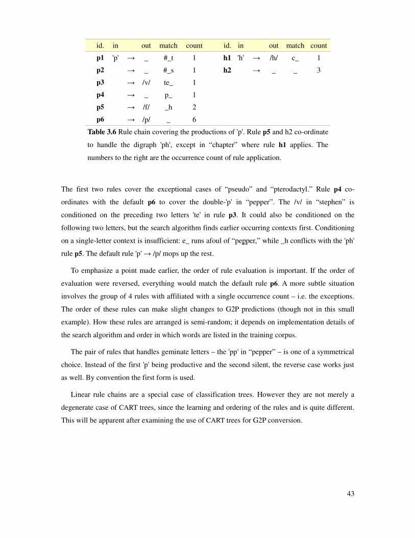
id. in out match count id. in out match count

p1 'p' → _ #_t 1 h1 'h' → /h/ c_ 1

p2 → _ #_s 1 h2 → _ _ 3

p3 → /v/ te_ 1

p4 → _ p_ 1

p5 → /f/ _h 2

p6 → /p/ _ 6

Table 3.6 Rule chain covering the productions of 'p'. Rule p5 and h2 co-ordinate

to handle the digraph 'ph', except in “chapter” where rule h1 applies. The

numbers to the right are the occurrence count of rule application.

The first two rules cover the exceptional cases of “pseudo” and “pterodactyl.” Rule p4 co-

ordinates with the default p6 to cover the double-'p' in “pepper”. The /v/ in “stephen” is

conditioned on the preceding two letters 'te' in rule p3. It could also be conditioned on the

following two letters, but the search algorithm finds earlier occurring contexts first. Conditioning

on a single-letter context is insufficient: e_ runs afoul of “pepper,” while _h conflicts with the 'ph'

rule p5. The default rule 'p' → /p/ mops up the rest.

To emphasize a point made earlier, the order of rule evaluation is important. If the order of

evaluation were reversed, everything would match the default rule p6. A more subtle situation

involves the group of 4 rules with affiliated with a single occurrence count – i.e. the exceptions.

The order of these rules can make slight changes to G2P predictions (though not in this small

example). How these rules are arranged is semi-random; it depends on implementation details of

the search algorithm and order in which words are listed in the training corpus.

The pair of rules that handles geminate letters – the 'pp' in “pepper” – is one of a symmetrical

choice. Instead of the first 'p' being productive and the second silent, the reverse case works just

as well. By convention the first form is used.

Linear rule chains are a special case of classification trees. However they are not merely a

degenerate case of CART trees, since the learning and ordering of the rules and is quite different.

This will be apparent after examining the use of CART trees for G2P conversion.

43

3.1.3 CART tree rules

Classification And Regression Tress are applicable to problems where the predicting features

of the domain are discrete and the predicted feature of the range is either discrete (classification)

or continuous (regression) [31]. CART trees are similar to rewrite rule chains but differ in three

respects. The first two points concern representative power and structure, while the third is tied to

implementation of the learning algorithm.

The decision rules are organized into a binary tree structure. Each interior node asks a

yes/no question of the domain features, and each leaf node is a prediction. Strictly, the

branching does not have to be binary – the questions can be 1-of-n choices – but the

binary constraint is a useful practical simplification (without loss of generality).

CART trees can easily make use of extra side information. Part-of-speech attributes is a

major category, in particular, such as is needed in English to make verb/noun distinctions

(e.g. the vowel alteration and stress shift of pro'ject/project'). As typically formulated,

linear rule chains use only the contextual information that is available in the grapheme

sequence.

The questions of CART trees can “jump around” the feature space in no particular order,

except that which the learning algorithm discovers to be most predictive. For example,

the “silent e” rule that applies to English word pairs “ban/bane,” and “bon/bone” can be

represented in a node that asks the question: “is the letter 2 places forward an 'e'?”.

The miniature corpus for the letter 'p' illustrates the contrast between CART trees rules and rule

chains. It's worth remembering that these structures are not unique. They depend on the

particulars of how the respective algorithms search the prediction space, on a stopping criteria,

the conventions for breaking ties – even the ordering of training samples and the ordering of the

features listed per example can have influence. Figure 3.1 is a CART tree that perfectly predicts

all twelve instances of the letter p. The words dangling off each leaf node indicates the rule

application.

44

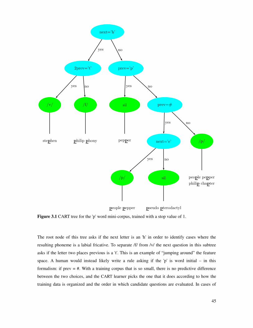
Figure 3.1 CART tree for the 'p' word mini-corpus, trained with a stop value of 1.

The root node of this tree asks if the next letter is an 'h' in order to identify cases where the

resulting phoneme is a labial fricative. To separate /f/ from /v/ the next question in this subtree

asks if the letter two places previous is a 't'. This is an example of “jumping around” the feature

space. A human would instead likely write a rule asking if the 'p' is word initial – in this

formalism: if prev = #. With a training corpus that is so small, there is no predictive difference

between the two choices, and the CART learner picks the one that it does according to how the

training data is organized and the order in which candidate questions are evaluated. In cases of

45

yes

no yes

no

yes no

yes no

yes no

prev=#sil/v/ /f/

/p/next=’e’stephen philip phony pepper

people pepper pseudo pterodactyl

prev=’p’2prev=’t’

next=’h’

people pepper

philip chapter

/p/ sil

ties there is not a learning bias that favors nearby letters. This is in contrast to our rule chain

learner, which does have a learning bias towards nearby contexts. Further explanation is

presented in the next section. The contrast can be illustrated with a tree representation of the rules

listed in Table 3.6. (For compactness, only the exception words are shown.)

Figure 3.2 Rule chain for the 'p'-word mini-corpus graphed as a CART tree. Interior (blue) nodes

show the context that is matched.

46

yesno

yesno

yesno

yesno

yesno

te

h

p /v/

sil stephen

/p/ /f/

pseudo

pterodactyl

pepper

sil

# s sil

# t

In both trees above there are five interior question nodes and six phone-producing leaf nodes.

But the organizational philosophies, in a manner of speaking, are diametrical. Rules chains

proceed from the most exception-specific questions to the more common cases. The first four

questions all apply to just one case in the training data, while the final question splits the pair of

/f/ p's from the six instances of /p/ (the default case). Let us call the number instances that a rule

encompasses with a yes node its “popularity.” In rule chains, the popularity of rule Ri+1 is always

less than or equal that of rule Ri, where R0 is the default rule. CART trees, in contrast, favors

questions that evenly split the data. Compare the question “is the next letter an 'h'?”. In Figure 3.2

the this is last non-default question asked; in Figure 3.1 it is the first question.

Always a concern with machine learning algorithms, including CART trees, is the prospect of

over-training. In the tree of Figure 3.1 greater regularity can be achieved by combining leaf

nodes, a process called merging. For example the /v/ and /f/ nodes on the left hand side can be

merged into one [53][73]. While it increases the error rate on the training set, the error rate is

often be reduced on test sets (thereby being less over-trained, by definition). An alternate way of

controlling over-training is during the initial tree-building process by defining a minimum node

size. When building the CART tree a policy is enforced that prohibits splitting a node if one of the

children would have fewer than the specified minimum size. The minimum node size is also

called the stop value. A stop value of 2 would prohibit the /v/-/f/ split, as well as the “pepper”

node from forming. This is seen in the Figure 3.3 below.

The figures that follow show increasingly reduced trees as achieved by setting the stop value

to 2, 3, 6, and 8. The last tree is the degenerate case: a single node that predicts the default /p/.

Inside the leaf nodes for these trees is a tuple, e.g. (6,2,1,3). This describes the number of cases of

/p, f, v, sil/ that is affiliated with the node after training. The predicted output symbol is the

maximum likelihood value – that is, the symbol with the largest count. When multiple symbols

share that same largest value, one is picked. The tie-breaking choice is dependent on the

implementation.

Linear rule chains can also be controlled during the build process with a stop value threshold,

or alternatively through post-pruning. The post-pruning operation simply removes nodes from the

tail (the most specific questions) one at a time. During building, a stop threshold of n prevent

nodes of fewer than n examples from forming. A stop value of 3 produces Figure 3.7. With three

nodes this is more compact than a CART tree of the same stop value, Figure 3.4, and is more

accurate on the data than the CART tree with the same number of nodes, i.e. Figure 3.5.

47

Figure 3.3 CART tree for the 'p'-word mini-corpus, trained with a stop value of 2.

Figure 3.4 CART tree for the 'p'-word mini-corpus, trained with a stop value of 3.

48

yes no

yes no

prev=#(0,2,1,0)

/f/

(4,0,0,1)

/p/

next=’h’

(2,0,0,2)

/sil/

yes no yes no

yes no

yes no

2prev=’e’next=’e’

(2,0,0,0)

/p/

(0,0,0,2)

sil

(3,0,0,0)

/p/

(1,0,0,1)

sil

prev=#(0,2,1,0)

/f/

next=’h’

Figure 3.5 CART tree for the 'p'-word mini-corpus, trained with a stop value of 6

Figure 3.6 Degenerate CART tree for the 'p'-word mini-corpus, trained with a stop value greater

than 6.

Figure 3.7 Rule chain with a single question, trained with a stop value of 3.

In the next section the error rates of these various rule systems is compared, in order to illustrate

the trade off between accuracy and rule set complexity.

49

yes no

(4,0,1,1)

/p/

(2,2,0,2)

sil

prev=’h’

(6,2,1,3)

/p/

no yes

(0,2,1,0)

/f/

(6,0,0,3)

/p/

h

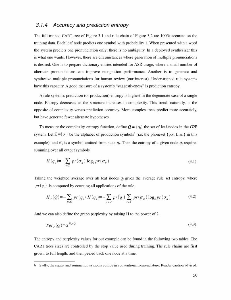
3.1.4 Accuracy and prediction entropy

The full trained CART tree of Figure 3.1 and rule chain of Figure 3.2 are 100% accurate on the

training data. Each leaf node predicts one symbol with probability 1. When presented with a word

the system predicts one pronunciation only; there is no ambiguity. In a deployed synthesizer this

is what one wants. However, there are circumstances where generation of multiple pronunciations

is desired. One is to prepare dictionary entries intended for ASR usage, where a small number of

alternate pronunciations can improve recognition performance. Another is to generate and

synthesize multiple pronunciations for human review (our interest). Under-trained rule systems

have this capacity. A good measure of a system's “suggestiveness” is prediction entropy.

A rule system's prediction (or production) entropy is highest in the degenerate case of a single

node. Entropy decreases as the structure increases in complexity. This trend, naturally, is the

opposite of complexity-versus-prediction accuracy. More complex trees predict more accurately,

but have generate fewer alternate hypotheses.

To measure the complexity-entropy function, define Q = qj the set of leaf nodes in the G2P

system. Let = i be the alphabet of production symbols6 (i.e. the phoneset p,v, f, sil in this

example), and ij is a symbol emitted from state qj. Then the entropy of a given node qj requires

summing over all output symbols.

H q j=−∑i∈

pr ij log2 pr ij (3.1)

Taking the weighted average over all leaf nodes qj gives the average rule set entropy, where

pr q j is computed by counting all applications of the rule.

H PQ=−∑j∈Q

pr q j H q j=−∑j∈Q

pr q j ∑i∈

pr ij log2 pr ij (3.2)

And we can also define the graph perplexity by raising H to the power of 2.

Per P Q=2H PQ (3.3)

The entropy and perplexity values for our example can be found in the following two tables. The

CART trees sizes are controlled by the stop value used during training. The rule chains are first

grown to full length, and then peeled back one node at a time.

6 Sadly, the sigma and summation symbols collide in conventional nomenclature. Reader caution advised.

50

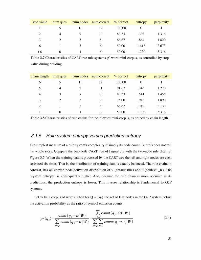
stop value num ques. num nodes num correct % correct entropy perplexity

1 5 11 12 100.00 0 1

2 4 9 10 83.33 .396 1.316

3 2 5 8 66.67 .864 1.820

6 1 3 6 50.00 1.418 2.673

>6 0 1 6 50.00 1.730 3.316

Table 3.7 Characteristics of CART tree rule systems 'p'-word mini-corpus, as controlled by stop

value during building.

chain length num ques. num nodes num correct % correct entropy perplexity

6 5 11 12 100.00 0 1

5 4 9 11 91.67 .345 1.270

4 3 7 10 83.33 .541 1.455

3 2 5 9 75.00 .918 1.890

2 1 3 8 66.67 1.080 2.133

1 0 1 6 50.00 1.730 3.316

Table 3.8 Characteristics of rule chains for the 'p'-word mini-corpus, as pruned by chain length.

3.1.5 Rule system entropy versus prediction entropy

The simplest measure of a rule system's complexity if simply its node count. But this does not tell

the whole story. Compare the two-node CART tree of Figure 3.5 with the two-node rule chain of

Figure 3.7. When the training data is processed by the CART tree the left and right nodes are each

activated six times. That is, the distribution of training data is exactly balanced. The rule chain, in

contrast, has an uneven node activation distribution of 9 (default rule) and 3 (context '_h'). The

“system entropy” is consequently higher. And, because the rule chain is more accurate in its

predictions, the production entropy is lower. This inverse relationship is fundamental to G2P

systems.

Let W be a corpus of words. Then for Q = qj the set of leaf nodes in the G2P system define

the activation probability as the ratio of symbol emission counts.

pr q j=count q j∣W

∑j∈Q

count q j∣W =

∑i∈

count q ji∣W

∑j∈Q

∑i∈

countq j i∣W (3.4)

51

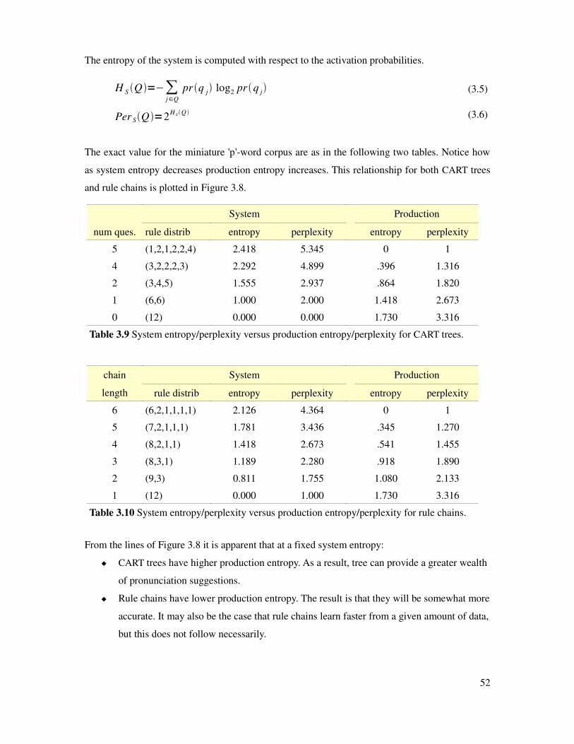
The entropy of the system is computed with respect to the activation probabilities.

H S Q=−∑j∈Q

pr q j log2 pr q j (3.5)

Per SQ=2H S Q (3.6)

The exact value for the miniature 'p'-word corpus are as in the following two tables. Notice how

as system entropy decreases production entropy increases. This relationship for both CART trees

and rule chains is plotted in Figure 3.8.

System Production

num ques. rule distrib entropy perplexity entropy perplexity

5 (1,2,1,2,2,4) 2.418 5.345 0 1

4 (3,2,2,2,3) 2.292 4.899 .396 1.316

2 (3,4,5) 1.555 2.937 .864 1.820

1 (6,6) 1.000 2.000 1.418 2.673

0 (12) 0.000 0.000 1.730 3.316

Table 3.9 System entropy/perplexity versus production entropy/perplexity for CART trees.

chain

length

System Production

rule distrib entropy perplexity entropy perplexity

6 (6,2,1,1,1,1) 2.126 4.364 0 1

5 (7,2,1,1,1) 1.781 3.436 .345 1.270

4 (8,2,1,1) 1.418 2.673 .541 1.455

3 (8,3,1) 1.189 2.280 .918 1.890

2 (9,3) 0.811 1.755 1.080 2.133

1 (12) 0.000 1.000 1.730 3.316

Table 3.10 System entropy/perplexity versus production entropy/perplexity for rule chains.

From the lines of Figure 3.8 it is apparent that at a fixed system entropy:

CART trees have higher production entropy. As a result, tree can provide a greater wealth

of pronunciation suggestions.

Rule chains have lower production entropy. The result is that they will be somewhat more

accurate. It may also be the case that rule chains learn faster from a given amount of data,

but this does not follow necessarily.

52

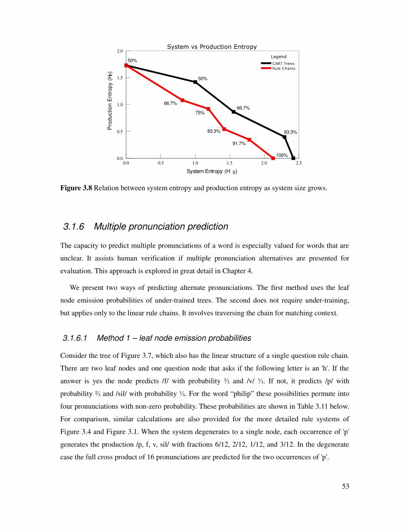
Figure 3.8 Relation between system entropy and production entropy as system size grows.

3.1.6 Multiple pronunciation prediction

The capacity to predict multiple pronunciations of a word is especially valued for words that are

unclear. It assists human verification if multiple pronunciation alternatives are presented for

evaluation. This approach is explored in great detail in Chapter 4.

We present two ways of predicting alternate pronunciations. The first method uses the leaf

node emission probabilities of under-trained trees. The second does not require under-training,

but applies only to the linear rule chains. It involves traversing the chain for matching context.

3.1.6.1 Method 1 – leaf node emission probabilities

Consider the tree of Figure 3.7, which also has the linear structure of a single question rule chain.

There are two leaf nodes and one question node that asks if the following letter is an 'h'. If the

answer is yes the node predicts /f/ with probability ⅔ and /v/ ⅓. If not, it predicts /p/ with

probability ⅔ and /sil/ with probability ⅓. For the word “philip” these possibilities permute into

four pronunciations with non-zero probability. These probabilities are shown in Table 3.11 below.

For comparison, similar calculations are also provided for the more detailed rule systems of

Figure 3.4 and Figure 3.1. When the system degenerates to a single node, each occurrence of 'p'

generates the production /p, f, v, sil/ with fractions 6/12, 2/12, 1/12, and 3/12. In the degenerate

case the full cross product of 16 pronunciations are predicted for the two occurrences of 'p'.

53

System Entropy (H S)

0.0 0.5 1.0 1.5 2.0 2.5

Pro

du

ctio

n E

ntr

op

y (

HP)

0.0

0.5

1.0

1.5

2.0System vs Production Entropy

Legend

CART Trees

Rule Chains

83.3%

66.7%

50%

83.3%

50%

66.7%

91.7%

100%

75%

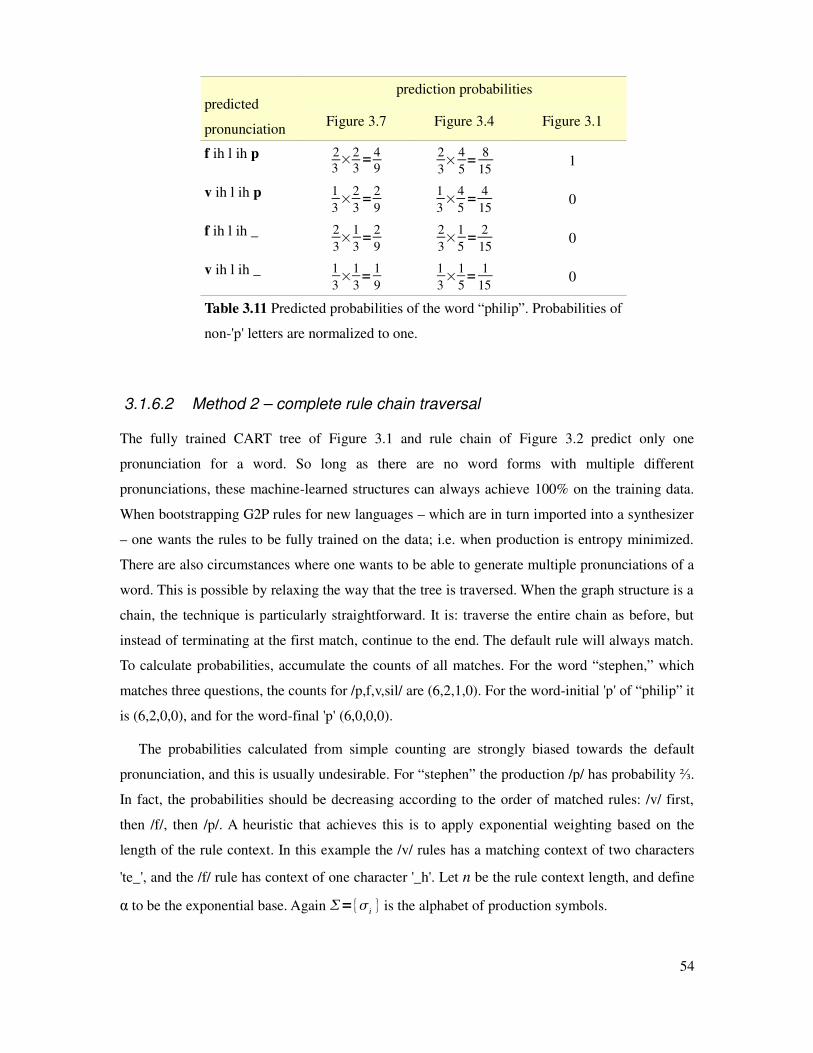
predicted

pronunciation

prediction probabilities

Figure 3.7 Figure 3.4 Figure 3.1

f ih l ih p 2

3×

2

3=

4

9

2

3×

4

5=

8

151

v ih l ih p 1

3×

2

3=

2

9

1

3×

4

5=

4

150

f ih l ih _ 2

3×

1

3=

2

9

2

3×

1

5=

2

150

v ih l ih _ 1

3×

1

3=

1

9

1

3×

1

5=

1

150

Table 3.11 Predicted probabilities of the word “philip”. Probabilities of

non-'p' letters are normalized to one.

3.1.6.2 Method 2 – complete rule chain traversal

The fully trained CART tree of Figure 3.1 and rule chain of Figure 3.2 predict only one

pronunciation for a word. So long as there are no word forms with multiple different

pronunciations, these machine-learned structures can always achieve 100% on the training data.

When bootstrapping G2P rules for new languages – which are in turn imported into a synthesizer

– one wants the rules to be fully trained on the data; i.e. when production is entropy minimized.

There are also circumstances where one wants to be able to generate multiple pronunciations of a

word. This is possible by relaxing the way that the tree is traversed. When the graph structure is a

chain, the technique is particularly straightforward. It is: traverse the entire chain as before, but

instead of terminating at the first match, continue to the end. The default rule will always match.

To calculate probabilities, accumulate the counts of all matches. For the word “stephen,” which

matches three questions, the counts for /p,f,v,sil/ are (6,2,1,0). For the word-initial 'p' of “philip” it

is (6,2,0,0), and for the word-final 'p' (6,0,0,0).

The probabilities calculated from simple counting are strongly biased towards the default

pronunciation, and this is usually undesirable. For “stephen” the production /p/ has probability ⅔.

In fact, the probabilities should be decreasing according to the order of matched rules: /v/ first,

then /f/, then /p/. A heuristic that achieves this is to apply exponential weighting based on the

length of the rule context. In this example the /v/ rules has a matching context of two characters

'te_', and the /f/ rule has context of one character '_h'. Let n be the rule context length, and define

α to be the exponential base. Again =i is the alphabet of production symbols.

54

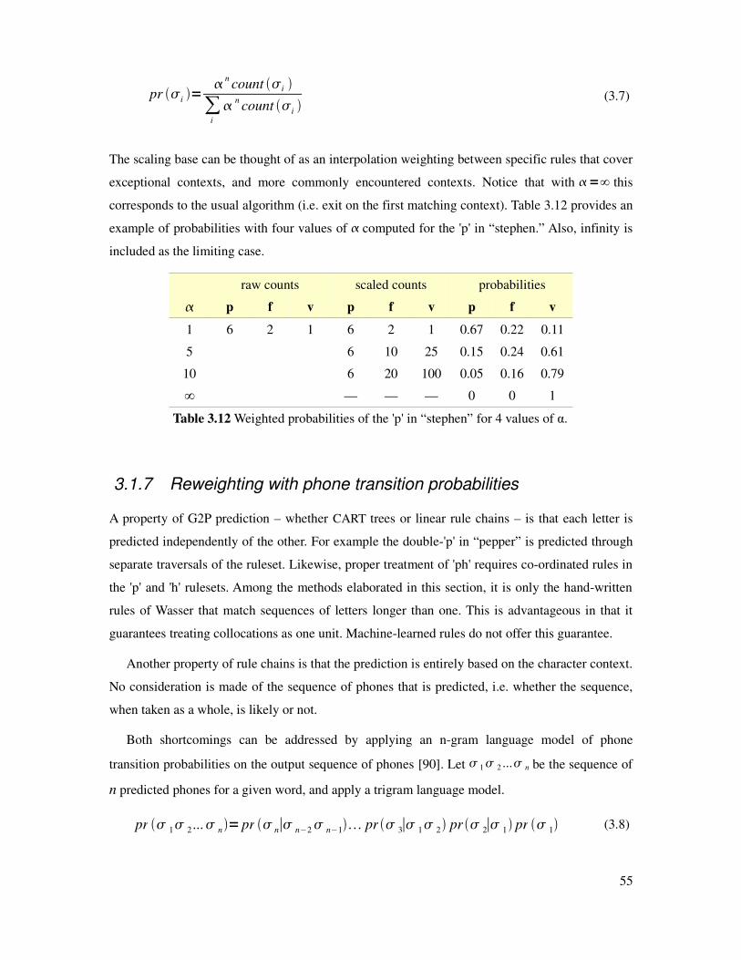
pr i = n

count i

∑i

ncount i

(3.7)

The scaling base can be thought of as an interpolation weighting between specific rules that cover

exceptional contexts, and more commonly encountered contexts. Notice that with =∞ this

corresponds to the usual algorithm (i.e. exit on the first matching context). Table 3.12 provides an

example of probabilities with four values of computed for the 'p' in “stephen.” Also, infinity is

included as the limiting case.

raw counts scaled counts probabilities

p f v p f v p f v

1 6 2 1 6 2 1 0.67 0.22 0.11

5 6 10 25 0.15 0.24 0.61

10 6 20 100 0.05 0.16 0.79

∞ — — — 0 0 1

Table 3.12 Weighted probabilities of the 'p' in “stephen” for 4 values of α.

3.1.7 Reweighting with phone transition probabilities

A property of G2P prediction – whether CART trees or linear rule chains – is that each letter is

predicted independently of the other. For example the double-'p' in “pepper” is predicted through

separate traversals of the ruleset. Likewise, proper treatment of 'ph' requires co-ordinated rules in

the 'p' and 'h' rulesets. Among the methods elaborated in this section, it is only the hand-written

rules of Wasser that match sequences of letters longer than one. This is advantageous in that it

guarantees treating collocations as one unit. Machine-learned rules do not offer this guarantee.

Another property of rule chains is that the prediction is entirely based on the character context.

No consideration is made of the sequence of phones that is predicted, i.e. whether the sequence,

when taken as a whole, is likely or not.

Both shortcomings can be addressed by applying an n-gram language model of phone

transition probabilities on the output sequence of phones [90]. Let 1 2 ... n be the sequence of

n predicted phones for a given word, and apply a trigram language model.

pr 1 2... n=pr n∣ n−2 n−1 pr 3∣ 1 2 pr 2∣ 1 pr 1 (3.8)

55

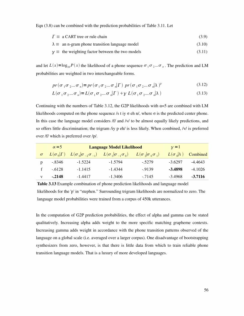
Eqn (3.8) can be combined with the prediction probabilities of Table 3.11. Let

≡ a CART tree or rule chain (3.9)

≡ an n-gram phone transition language model (3.10)

≡ the weighting factor between the two models (3.11)

and let L x =log10 P x the likelihood of a phone sequence 1 2 ... n . The prediction and LM

probabilities are weighted in two interchangeable forms.

pr 1 2... n=pr 1 2 ... n∣ pr 1 2 ... n∣ (3.12)

L 1 2 ... n=L 1 2 ... n∣ L 1 2 ... n∣ (3.13)

Continuing with the numbers of Table 3.12, the G2P likelihoods with α=5 are combined with LM

likelihoods computed on the phone sequence /s t iy σ eh n/, where σ is the predicted center phone.

In this case the language model considers /f/ and /v/ to be almost equally likely predictions, and

so offers little discrimination; the trigram /iy p eh/ is less likely. When combined, /v/ is preferred

over /f/ which is preferred over /p/.

=5 Language Model Likelihood =1

L 0∣ L 0∣ −2 −1 L 1∣ −1 0 L 2∣ 0 1 L 0∣ Combined

p -.8346 -1.5224 -1.5794 -.5279 -3.6297 -4.4643

f -.6128 -1.1415 -1.4344 -.9139 -3.4898 -4.1026

v -.2148 -1.4417 -1.3406 -.7145 -3.4968 -3.7116

Table 3.13 Example combination of phone prediction likelihoods and language model

likelihoods for the 'p' in “stephen.” Surrounding trigram likelihoods are normalized to zero. The

language model probabilities were trained from a corpus of 450k utterances.

In the computation of G2P prediction probabilities, the effect of alpha and gamma can be stated

qualitatively. Increasing alpha adds weight to the more specific matching grapheme contexts.

Increasing gamma adds weight in accordance with the phone transition patterns observed of the

language on a global scale (i.e. averaged over a larger corpus). One disadvantage of bootstrapping

synthesizers from zero, however, is that there is little data from which to train reliable phone

transition language models. That is a luxury of more developed languages.

56

3.1.8 Rule learning architectures: pros and cons

In this chapter we've examined three G2P rule architectures: rule chains that support a multi-

character left hand side in the rules plus special regular expressions as matching context string

(section 3.1.1), rule chains restricted to single character left hand sides (section 3.1.2), and CART

trees with single character questions (section 3.1.3). The first choice has the advantage of being

the most compact, since the rules can operation on items more general than string literals. The

downside is that this compounds the difficulty of automatically learning rewrite rules.

While we've adopted linear rule chains of the second, more concrete variety, CART trees have

undeniable advantages. They are more general in their learning capability. This is exhibited in

their capacity to jump letter positions, and in being able to use extra features such as parts of

speech tags. CART trees are faster to apply; for N total nodes the average depth is d ~log2 N

assuming a balanced branching structure. Also, when the trees are undertrained, it can be argued

that the leaf node probability distribution functions are better than those of rule chains.

On the other hand, multiple pronunciations can be generated from rule chains by the technique

of full traversal matching, i.e. without needing a second, smoother rule set. We have also found

that rule chains provide slightly superior prediction accuracy (cf. section 3.3.2 ). The precise

reason why is not easy to pin down, especially in systems containing thousands of nodes, but we

attribute it to a superior induction bias. On account of the learning algorithm's search policy

(explained in the next section), the induction bias is tilted towards local character contexts. This is

the flip side of CART tree's ability to “jump around.” On balance, searching for explanatory

contexts close to the center character results in rules that extrapolate better to unseen words. At

the practical level we have found that our CART learning implementation is somewhat sensitive

to the particulars of how the features are organized in the training data file. In the rule chain

learner these vagaries are accommodated in the algorithm's search policy.

A final, major practical advantage of rule chains over CART trees is the ability to support

incremental updates. This is the ability to incrementally revise the rules with the addition of each

word/pronunciation pair provided by the user. In an online learning system where immediate

feedback is expected, this is a highly desirable property. It becomes increasingly critical as the

lexicon grows in size and consequently the G2P learning time increases to minutes or more.

Davel and Barnard have shown there is little loss in prediction accuracy with incremental

updating, provided that every for 50-100 rule alterations the system periodically performs a

complete rebuild from scratch (a batch operation) [50]. To be fair, all this is unnecessary in the

57

presence of sufficiently fast computers – one could rebuild the G2P rules from scratch every time.

One could also invest intensive engineering effort into code optimization, including multi-

threading and parallelization on computing clusters. Currently, the method incremental updates

with periodic rebuilds is a cheaper, more practical solution.

With our survey of methods and general discussion complete, the setting is now prepared for a

more formal description how G2P rule chains are learned automatically from data.

3.2 G2P rule learning

G2P rule learning consists of two phases. First is the task of finding the most probable alignment

between the graphemes and phonemes of a set of words. Alignment determines the specific

grapheme to phoneme productions. To present a “phony” example:

p h o n y

↓ ↓ ↓ ↓ ↓

ph sil ow n iy

From these, the aligned training data determines G2P probability distribution functions of eqn

(3.4). Each grapheme's pdf is independent of neighboring context. The maximum likelihood

production for each grapheme is its default rule. This is equivalent to the highest-entropy, single-

node G2P rule system illustrated in Figure 3.6.

The second stage is to define the default system into rule chains or CART trees that

incorporate contextual predictions. As explained in section 3.1.5 the production entropy decreases

at the expense of increasing system complexity.

The techniques applied to these two problems are iterative Viterbi alignment and dynamic

expanding context (DEC) search. Iterative Viterbi is well suited to aligning two symbol streams

from a flat start [3]. Flat start initialization (where every grapheme is equally likely to produce

every phoneme) is prone to converging on a suboptimal local minima. To improve the prospect of

finding a good solution we introduce a novel way of ordering the training data. Following

alignment, we apply a modified version of the DEC search strategy advocated by [162]. Our

modification trades off some computational efficiency (by operating is a less constrained search

space) for slightly higher accuracy and learning efficiency.

To describe these procedures it helps to introduce formal notation.

58

3.2.1 Formal definition of G2P rules

We have already introduced Q = qj as the set of states in a G2P system, and sigma =i is

the alphabet of production symbols (phonemes), with j=

ij the symbols emitted at state j. A

lexicon L, is a 3-tuple of vocabulary, phonetization, and source: L = (V, P, S). The source field

provides annotation to disambiguate homographs. If the corpus contains the sentence “the wind

turned the bow shoreward” then the lexicon benefits from entries such as listed.

V P S Σn

bow b ow archer b,ow

bow(2) b aw canoe aw,b,ow

shoreward sh ao r w er d –– ao,aw,b,d,er,ow,r,sh,w

the th iy formal ao,aw,b,d,er,iy,ow,r,sh,th,w

the(2) th ax common ao,ax,aw,b,d,er,iy,ow,r,sh,th,w

turned t er n d –– ao,ax,aw,b,d,er,iy,n,ow,r,sh,t,th,w

wind w ih n d noun ao,ax,aw,b,d,er,ih,iy,n,ow,r,sh,t,th,w

wind(2) w ay n d verb ao,ax,aw,ay,b,d,er,ih,iy,n,ow,r,sh,t,th,w

Table 3.14 Small lexicon with annotations. The phoneset is updated one word at a time.

The algorithms for performing alignment and rule learning are iterative with respect to lexicon

growth. The lexicon can grow due to external factors such as the user supplying additional text to

the system. It also grows “internally” in the sense that the active vocabulary starts empty and

grows as words are fed in. We use superscript n – Ln ,V n , Pn , n=in – to indicate iterative

version of the active data. Correspondingly, let n=in be the character set at iteration n.

With this notation and previous examples serving as background, we define a G2P system as

an ordered 8-tuple

G2P=Q , , , A ,B , R , q0 ,F (3.14)

where q0 is a start state and F is a final accepting state, A is a transition matrix, B an emission

matrix, and R the ruleset.

Q≡set of states (3.15)

≡character set (3.16)

≡ phoneset (3.17)

59

A :a ijk :qi , q j , Bool [0,1], ∑j

a ijk=1 (3.18)

B :bij : q i , j [0,1], ∑j

bij=1 (3.19)

R :r i :...−2 ,−1 ,0 ,1 ,2 ... False , True

r i :lc , mc , rcBool , mc=0

(3.20)

q0≡initial state (3.21)

F≡set of final accepting states (3.22)

In eqn (3.20) lc, mc, rc are left context, matching context, and right context, respectively. In our

machine learned rules the matching context is a single grapheme.

It may help clarify to compare to the 5-tuple definitions of Deterministic Finite Automata and

Hidden Markov Models. A DFA has a transition matrix δ that corresponds to A in an HMM, and a

start state q0 which corresponds to an initial probability distribution π. DFAs in this formulation

do not emit symbols.

DFA=Q , , , q0 ,F (3.23)

HMM=Q , A , B , , F (3.24)

Similar to a discrete HMM, a G2P model has an emission matrix B. The interior (blue colored)

nodes in our diagrams are non-emitting. For mathematical consistency these emit an epsilon

symbol with probability 1 (which is considered distinct from the silence symbol sil).

The transition matrix A is different from the DFA and HMM versions in that the transition

from qi to qj depends on the boolean rule evaluated at state qi. The probability distributions are

indicator functions. For either of True or False evaluations, only one destination state qj has

probability 1. Graphically, each internal, rule-asking node branches into two other nodes.

The set of states Q are divided in practice into disjoint subtrees with one tree dedicated to each

grapheme. These are connected via a “central station” distribution node. The distribution node

reads a character from the input stream and transitions to the appropriate subgraph. Internally, the

distribution node is itself a subgraph that asks a chain of questions: “is the current letter an 'a'? ...

is it a 'b'? ... and so on. At a higher level it is correctly viewed as an n-way case switch.

The emitting leaf nodes transition to the start state, whereupon another character is consumed.

Continuing our running example, a simple network capable of processing the word “philip”

follows in Figure 3.9. The nodes colored yellow constitute the n-way subgraph switch.

60

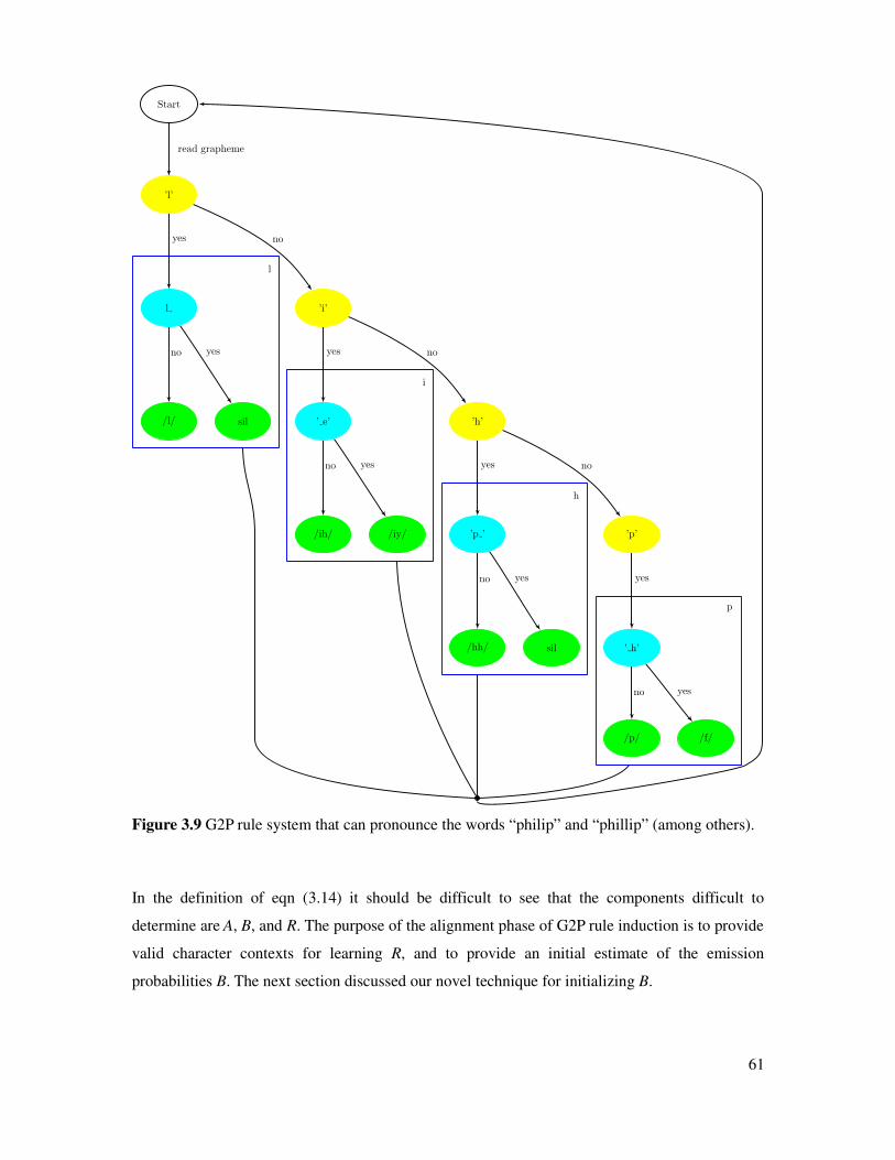
Figure 3.9 G2P rule system that can pronounce the words “philip” and “phillip” (among others).

In the definition of eqn (3.14) it should be difficult to see that the components difficult to

determine are A, B, and R. The purpose of the alignment phase of G2P rule induction is to provide

valid character contexts for learning R, and to provide an initial estimate of the emission

probabilities B. The next section discussed our novel technique for initializing B.

61

p

h

i

l

no

no yes

yes

noyes

yes no

read grapheme

yes

no

yes

yes yes

no

no

’l’

/hh/ sil

/iy//ih/

/l/ sil

/p/ /f/

’ h’

Start

l

’ e’

’p ’

’i’

’p’

’h’

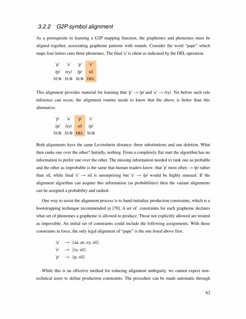
3.2.2 G2P symbol alignment

As a prerequisite to learning a G2P mapping function, the graphemes and phonemes must be

aligned together, associating grapheme patterns with sounds. Consider the word “pape” which

maps four letters onto three phonemes. The final 'e' is silent as indicated by the DEL operation.

'p' 'a' 'p' 'e'

/p/ /ey/ /p/ sil

SUB SUB SUB DEL

This alignment provides material for learning that 'p' → /p/ and 'a' → /ey/. Yet before such rule

inference can occur, the alignment routine needs to know that the above is better than this

alternative.

'p' 'a' 'p' 'e'

/p/ /ey/ sil /p/

SUB SUB DEL SUB

Both alignments have the same Levinshtein distance: three substitutions and one deletion. What

then ranks one over the other? Initially, nothing. From a completely flat start the algorithm has no

information to prefer one over the other. The missing information needed to rank one as probable

and the other as improbable is the same that human readers know: that 'p' most often → /p/ rather

than sil, while final 'e' → sil is unsurprising but 'e' → /p/ would be highly unusual. If the

alignment algorithm can acquire this information (as probabilities) then the variant alignments

can be assigned a probability and ranked.

One way to assist the alignment process is to hand-initialize production constraints, which is a

bootstrapping technique recommended in [70]. A set of constraints for each grapheme declares

what set of phonemes a grapheme is allowed to produce. Those not explicitly allowed are treated

as impossible. An initial set of constraints could include the following assignments. With these

constraints in force, the only legal alignment of “pape” is the one listed above first.

'a' → aa, ae, ey, sil

'e' → iy, sil

'p' → p, sil

While this is an effective method for reducing alignment ambiguity, we cannot expect non-

technical users to define production constraints. The procedure can be made automatic through

62

the incorporation of two techniques: 1) iterative Viterbi training, and 2) a sequencing pattern we

call “minimum-length-mismatch initialization heuristic.” Iterative Viterbi training is a well

known form of Expectation Maximization (EM) [61][120] and has been previously applied to

G2P alignment [3]. It works through a repeated two-stage procedure: aligning the data with the

current production probabilities B, then updating the probabilities with the current alignment

(which will usually be an improvement over the previous alignment). Our minimum-length-

mismatch initialization provides the first Viterbi stage with a good starting point.

The heuristic is based on the observation that equal length word/pronunciation pairs are the

most reliable source of alignment information. While “pape” is not such a word because four

letters map to three phonemes, the word “papa” is. It provides two examples each of 'p' → /p/ and

'a' → /aa/. This one-to-one mapping heuristic does not always hold – a counterexample is the

word “faxing” – but it holds predominantly, and that is sufficient for good initial probabilities.

Let a set of equal length word/pronunciation pairs be L, and g a mapping between them.

L=word k , pronunk =kl , kl (3.25)

g kl = kl (3.26)

The initial G2P system has one state per grapheme. Therefore the set of graphemes are in

correspondence with the set of states and each state's emission probabilities.

i ⇔qi⇔b i i=1∣∣ (3.27)

From the one-to-one correspondences of eqn (3.26) and eqn (3.27) we get initial production

probabilities through straightforward counting.

bij=∑k , l

count w k , l∣w k ,l=i , g w k ,l= i

∑k ,l

count w k ,l∣w k , l=i (3.28)

Through experimentation we have found that three-letter words provide a good initial vocabulary

V 0 . We partition the training data into a two dimensional grid of cells. Each word/pronunciation

training pair is assigned a two-tuple (len(word), len(pronunciation)). By this assignment, cell(3,3)

consists of all three-letter words that have three-phonemes, and cell(3,4) are three-letter words

with four-phonemes. Cell(4,*) contains all four letter words.

In our alignment algorithm, Viterbi alignment is applied multiple times on the lexicon,

63

incrementally accumulating data on a cell-by-cell basis. The order that the words in a cell are

visited and accumulated determines the visitation pattern.

V0 B

0Viterbi

V1B

1Viterbi

V2 B

2Viterbi

(3.29)

V0=w

3,3 (3.30)

V 1=V 0∪w3,2 (3.31)

V 2=V 1∪w3,4 (3.32)

V6=V

5∪w2,2 (3.33)

In our minimum-length-mismatch heuristic cells below the x=y line (fewer phonemes than

graphemes) are visited before cells above the x=y line. This should be clear in the table below.

All cells for words of a given length are accumulated before visiting longer or shorter words.

Table 3.16 provides representative examples of words for the first 15 visited cells.

7 20 25

nu

mb

er o

f p

ho

nem

es

6 19 23

5 5 17 21

4 10 3 15 22

3 14 8 1 16 24

2 13 6 2 18

1 11 7 4

0 12 9

1 2 3 4 5

length of word

Table 3.15 One cell visitation pattern of minimum-length-

mismatch ordering.

cell production cell production cell production

1. (3,3) bat → /b ae t/ 6. (2,2) at → /ae t/ 11. (1,1) a → /ey/

2. (3,2) ape → /ey p/ 7. (2,1) eh → /ey/ 12. (1,0) - → sil

3. (3,4) sox → /s aa k s/ 8. (2,3) ox → /aa k s/ 13. (1,2) b → /b iy/

4. (3,1) eye → /ay/ 9. (2,0) :) → sil 14. (4,4) cats → /k ae t s/

5. (3,5) abc → /ey b iy c iy/ 10. (2,4) cc → /s iy s iy/ 15. (4,3) pape → /p ey p/

Table 3.16 Examples of word from the cell visitation ordering of Table 3.15.

64

Experience has proven that this is a reliable heuristic for initializing and updating grapheme to

phoneme production probabilities (others work too). The visitation pattern can be viewed as an

answer to the question: what is the optimal ordering of of training samples to support reliable

joint discovery of word alignments G2P production probabilities? Or from the perspective of the

human user, what is the best ordering of word that minimized their effort? In section section 3.4

we engage the question of optimal word ordering to support G2P rule discovery.

3.2.3 Search strategy for rule learning

Once a default rule system is created from the alignment procedure, the next stage refines the

ruleset. The rules are refined in accordance with the most informative surrounding contexts. The

default rules have a context width of one (the grapheme itself), while each additional grapheme

increases the width of the context window. For example, if we are considering the first occurrence

of 's' in the word “basics,” the context windows are as listed in Table 3.17. Graphemes closer to

the word boundary have contexts that grow asymmetrically, as shown on the right side. When

learning lexical G2P rules, the training data does not contain contexts spanning across words.

Learning post-lexical rules due to cross-word influence requires spanning the contexts across

words, but this is not treated in the current discussion.

width context sets ordered by increasing width

1 _ _

2 a_ , _i #_ , _h

3 ba_ , a_i , _ic #_h, _hi

4 #ba_ , ba_i , a_ic , _ics #_hi, _hil

5 #ba_i , ba_ic , a_ics , _ics# #_hil, _hili

6 #ba_ic , ba_ics , a_ics# #_hili, _hilip

7 #ba_ics , ba_ics# #_hilip, _hilips

8 #ba_ics# #_hilips, _hilips#

9 #_hilips#

Table 3.17 Letter contexts for the first 's' in “basics” and first 'p' in “philips.”

The underscore character denotes the current position, while the hash marks

word boundary.

For the first 's' of “basics” there are 20 possible explanatory contexts, including the default. For

the first 'p' of “philips” there are nine explanatory context. Since the default rule is 'p' → p / _ but

the first 'p' in “philips” produces /f/ the rule learning algorithm notes the contradiction looks to

65

the remaining eight contexts for explanation. Considering this word alone each could just as well

explain the /f/ production, since each matches once. Given what we know of the relationship

between orthography and pronunciation, 'p' → f / _hilips# is not on equal standing with 'p' → f /

_h. (The overly specific choice violates Occam's razor.) The order in which contexts are visited

defines an algorithm's search strategy. The most popular search strategy for G2P learning is

“dynamically expanding context” or DEC. The DEC algorithm first searches contexts of length 1,

then those of length 2, then length 3, and so on, dynamically expanding from the current position.

DEC search strategies subdivide into variants depending on the exact order of context

visitation. Three possibilities are:

center-left-right ordering, shown below on the left side

center-right-left ordering, the reverse of the above

left-to-right sliding window, shown below on the right side

1 1

2 2

3

4 3

5

6

7 4

8

9

10

11 5

A search strategy is one half of a specification. An algorithm must also have a rule selection

policy. When combined with the search strategy, a policy for selecting one explanatory contexts

over other candidates is the algorithm's learning bias. Three possibilities include:

1. Select the first context found that explains the production.

2. Examine all contexts of a given width (e.g. ab_, a_b and _ab for width=3), and select the

best scoring context.

3. Examine all contexts at multiple widths, then select the best scoring context.

66

A policy of accepting the first matching context along with a center-left-right DEC search

strategy was the proposal of Torkkola (1993) [162]. Davel and Barnard improved on this using

policy 2 in combination with a left-center-right search strategy [47]. If all contexts of a given

width are examined before making a selection, then, as they point out, the detailed search order

does not matter. In our algorithm we employ the third policy: contexts of multiple widths are

examined as a group before making a selection. Through experimentation we found that if the

largest context window used in the rule chain for the currently grapheme is w, then contexts of

both w and w+1 should be searched. The advantage of this rule selection policy was also

discovered independently by Davel and Barnard [49]. Because grapheme contexts of unequal

width are examined as a group, rule chains do not obey a strict order of expanding windows,

though shorter contexts generally precede longer ones in the rule chains when starting from the

default. What remains to be specified is the means for determining the “best” context.

Consider the situation where a rule chain for 'p' contains only the default rule and we want to

extend it to cover more words. Table 3.18 shows eight possible explanatory grapheme contexts:

four of width 2, and four of width 3.

prod. context

new

right

new

wrong

no

diff

delta

score

total

score newly misclassified graphemes

'p'→ /f/ #_ 2 2 8 0 6 people, pepper

_h 2 0 10 +2 8 (stephen already wrong)

_s 0 1 11 -1 5 pseudo

_t 0 2 10 -2 4 pterodactyl, chapter

#_h 2 0 10 +2 8

_he 0 1 11 -1 5 stephen

_hi 1 0 11 +1 7

_ho 1 0 11 +1 7

Table 3.18 Some candidate contexts for explaining the production 'p'→ /f/.

Each candidate context is evaluated according to how it affects the overall classification accuracy

of the rule chain, were it hypothetically added to the system. Conditioning on “#_” (word start)

will classify “philip” and “phony” correctly when they were not so before, but undoes the

classification of “people” and “pepper.” The net gain is zero. Two contexts result in a maximal

net gain of 2: “_h” and “#_2”. The tie is broken by choosing the first option – it is shorter and

thus more general. If two contexts have the same width, then the context that is most central is

67

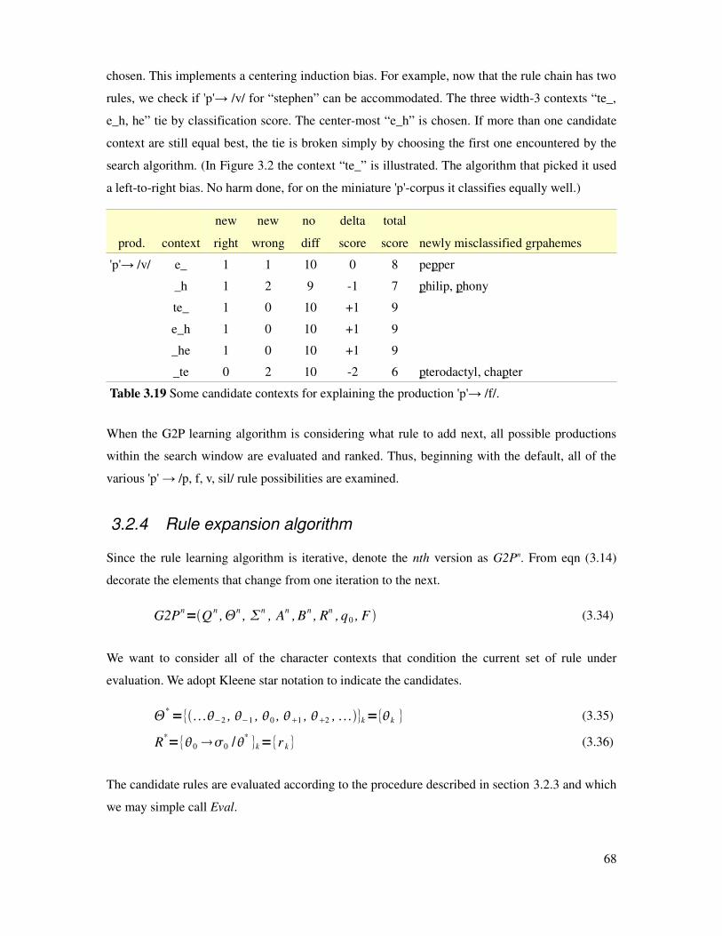
chosen. This implements a centering induction bias. For example, now that the rule chain has two

rules, we check if 'p'→ /v/ for “stephen” can be accommodated. The three width-3 contexts “te_,

e_h, he” tie by classification score. The center-most “e_h” is chosen. If more than one candidate

context are still equal best, the tie is broken simply by choosing the first one encountered by the

search algorithm. (In Figure 3.2 the context “te_” is illustrated. The algorithm that picked it used

a left-to-right bias. No harm done, for on the miniature 'p'-corpus it classifies equally well.)

prod. context

new

right

new

wrong

no

diff

delta

score

total

score newly misclassified grpahemes

'p'→ /v/ e_ 1 1 10 0 8 pepper

_h 1 2 9 -1 7 philip, phony

te_ 1 0 10 +1 9

e_h 1 0 10 +1 9

_he 1 0 10 +1 9

_te 0 2 10 -2 6 pterodactyl, chapter

Table 3.19 Some candidate contexts for explaining the production 'p'→ /f/.

When the G2P learning algorithm is considering what rule to add next, all possible productions

within the search window are evaluated and ranked. Thus, beginning with the default, all of the

various 'p' → /p, f, v, sil/ rule possibilities are examined.

3.2.4 Rule expansion algorithm

Since the rule learning algorithm is iterative, denote the nth version as G2Pn. From eqn (3.14)

decorate the elements that change from one iteration to the next.

G2Pn=Qn

,n, n

, An

, Bn, R

n, q0 , F (3.34)

We want to consider all of the character contexts that condition the current set of rule under

evaluation. We adopt Kleene star notation to indicate the candidates.

*=−2 , −1 , 0 , 1 , 2 , k=k (3.35)

R*=0 0 /

* k=r k (3.36)

The candidate rules are evaluated according to the procedure described in section 3.2.3 and which

we may simple call Eval.

68

r max=argmax Eval R* , r max=0 0 / lc _ rcmax (3.37)

When a maximal rule is identified, two new states (nodes) are created: qhead and qleaf. The context

of the new rule rmax is affiliated with the new head node, and the production is affiliated with the

leaf. If the rule introduce new graphemes or phonemes not previously seen, then the charset and

phoneset are expanded.

n1=n ∪0 charset expansion (3.38)

n1=n∪ 0 phoneset expansion (3.39)

Qn1=Q

nqhead , qtail , ∣Qn1∣=∣Qn∣2 state space expansion (3.40)

qhead lc _ rc head node assigned context (3.41)

q leaf 0 leaf node assigned phoneme (3.42)

The new nodes are connected to the rest of the network through the transition matrix A. Assume

an index function that returns the index number of a state. If the context assigned to the new head

node evaluates to True, the G2P transitions to the new leaf node. If False, it transition to the old

head node, which asks the next context question.

a i , j1 ,T =1, i=index qhead , j1=index q tail connect to new leaf (3.43)

a i , j ,T =0, j≠ j1

a i , j0 , F =1, i=index qhead , j0=index qoldhead connect to old head (3.44)

a i , j , F =0, j≠ j 0

An1=AN2, N2 , A

n=AN , N , A0=A1,1 matrix size expansion (3.45)

The emission probabilities are updated from the search process such that the maximum likelihood

phoneme is the symbol produced by the learned rule, i.e. 0 : rmax

=0 0 / lc _ rc .

Bn1bi :argmax jb ij= 0 , i=index q leaf update probabilities (3.46)

Combining the tasks of alignment and rule induction, the G2P algorithm has much to consider.

The algorithm's time complexity is polynomial in lexicon size, but is still fast enough for practical

application.

69

3.2.5 Learning algorithm speed

A theoretical analysis of the learning algorithm's computational complexity is not easily obtained.

An empirical measurement of training times, though, lends a favorable impression. Figure 3.10

compares the runtime of our G2P rule chain learner with wagon, the CART tree learner bundled

with the Edinburgh Speech Tools [67]. The program wagon operates in two modes which, for

current purposes, are fast (single pass) and slow (stepwise). A consideration to bear in mind is

that while wagon is a compiled C++ program, our G2P rule chain learner is implemented purely

in python, an interpreted language.

Figure 3.10 Comparison of G2P learner run times with that of wagon, a CART tree learner.

Measurements were performed on a 1.8 GHz Pentium 4.

Throughout this discussion of G2P rule learning, we have used for illustration a miniature corpus

of a mere eight words. Now we examine rule systems trained from data that contain thousands, or

even tens of thousands of rules. In the experiment of Figure 3.10 the largest run contained 320k

lexical entries.

70

1 week

Num Training Words

100 1000 10000 100000 1000000

Learning Tim

e (s)

0.1

1

10

100

1000

10000

100000

G2P Learning Time vs Corpus Size

1 min

1 day

1 hour

Italian

Wagon Stepwise, stop=3

Wagon Single pass, stop=3

Rule chain learner

3.3 G2P performance across languages

Languages differ in the complexity of the relation between orthography and phonology. English is

notorious for having a highly irregular spelling system. Conversely, Spanish and Portuguese are

admired for their simplicity. Most others lie somewhere in between. This section surveys a range

of languages with a view towards the following questions.

1. For a given language how large is its rule system?

2. How quickly are the G2P rules of a languages learned? How many words are required to

learn the system to 90 or 95% accuracy?

3. When does the size of a rule system plateau (reach an asymptote) as the training lexicon

increases in size?

4. What is the prediction accuracy of a rule system as it grows?

5. What is the distribution of context widths among the individual rules?

Perhaps surprisingly, experiments demonstrate that the size of a language's rule system does not

asymptote, but grows without bound, exhibiting a power law relationship. The rule system

complexity across languages is compared using the perplexity formula of eqn (3.6).

3.3.1 A test suite of eight languages

Our test suite consists of pronunciation dictionaries from seven languages, with English

considered under two manifestations.

English. Version 0.6d of CMU-DICT, considered without stress (39 phones) and with

two level stress marking (58 phones) [42].

German. The Celex dictionary of 321k entries (Burnage, 1990) [36].

Dutch. The Fonilex dictionary of 218k entries (Mertens and Vercammen, 1998) [74].

Fonilex defines an abstract phonological level from which specific dialects are specified.

We tested on the “standard” dialect.

Afrikaans. A 37k dictionary developed locally. Afrikaans is a language of South Africa

and is a recent derivative of Dutch [1].

Italian. A large 410k dictionary distributed as part of a free Festival-based Italian

synthesizer [44].

71

Spanish. Generated by applying a set of hand written rules to a 52k lexicon. The G2P

rules are a part of the standard Festival Spanish distribution [69]. In effect, our rule

learner is attempting to infer the original rules by way of production data.

Telugu. An 8k locally developed dictionary. In its native orthography, this language of

India possess a highly regular syllabic writing system. We've adopted a version of the

Itrans-3 transliteration scheme in which sequences of two to four English letters map onto

Telugu phonemes [109].

Iraqi Arabic. A 40k dictionary of “unvowelized” word forms. This dictionary is

extensively treated in Chapter 4.

3.3.2 Empirical measurements

While Spanish hardly requires machine-learned G2P rules, Spanish in Figure 3.11 illustrates a

characteristic pattern. The x-axis is the total number of rules as they are added one by one. The

y-axis is the percentage of correctly predicted letters and words, respectively, evaluated on the

training data. Because rule chains are extended by greedily selecting the candidate rule that

provides the largest improvement in character prediction, the character accuracy is a

monotonically increasing curve. The word accuracy is mostly increasing, but can momentarily

decrease before resuming upward.

Figure 3.11 Coverage of Spanish (52k corpus) as a function of rule size. For the lower curve W

indicates the maximum context window width. The middle curve tracks near-optimal

performance improvement with the introduction of new rules.

72

Legend

Chars Correct

Words Correct

Words Correct

Number of Rules

0 10 20 30 40 50 60

Percent Correct

0

20

40

60

80

100Spanish LTS Ruleset Performance

W=3W=2W=1

In the lower curve of Figure 3.11 the growth procedure is constrained such that all width-1 rules

are added before width-2 rules, which in turn must be exhausted before width-3 rules are

considered. This constraint leads to the curve's distinctive scalloped shape. The upper limit of the

W=1 region shows the performance of the default rules alone (68% words correct).

For more complex languages the majority of rules have a context width in the range of 3 to 6.

This is seen in Figure 3.12 for English, Dutch, Afrikaans, and Italian. However, a larger rule set

does not mean that the average context width is greater. In the next table compare Italian to Dutch

(4.78 vs. 4.35). See also the summary statistics of Table 3.21.

language number of rules average width

English 40k 19231 5.06

Dutch 40k 10071 4.35

Afrikaans 37k 5993 4.66

Italian 40k 3385 4.78

Spanish 52k 76 1.66

Table 3.20 Number of G2P rules for five language and their average

context width.

Figure 3.12 Distribution of G2P rules by context window width for four languages: English,

Dutch, Afrikaans, and Italian.

73

Window Width

2 4 6 8 10

Number of Rules

0

1000

2000

3000

4000

5000

6000LTS Rule Count vs Window Width

Legend

English 40k

Dutch 40k

Afrikaans 37k

Italian 40k

Figure 3.13 Example of growth of n-grams and rules for Afrikaans of Table 3.21 below.

Item Spanish Afrikaans Dutch English

# words 51476 36797 40000 40817

# graphemes 33 33 69 28

# bigrams 674 546 1082 661

# trigrams 5470 5275 8814 6206

# phonemes 25 34 45 39

# allowables 43 219 457 289

# trigger words 38 167 332 232

# G2P rules 74 5994 10071 19231

max window 3 20 14 16

Table 3.21 Summary statistics of four languages. Allowables are the unique

G2P productions (ignoring context). Trigger words are the minimal in-order set

covering all allowable productions.

Beyond a window width of 7, rule growth tapers off considerably. In this region most new rules

serve to identify particular words of irregular spelling, as it is uncommon for long rules to

generalize beyond a single instance. Thus when training a smoothed G2P rule system it is fair to

ignore contexts larger than 7, as is done in the Festvox synthesis building tool suite [70].

74

Num Words in Lexicon

100 1000 10000 100000

Occurance Count

1

10

100

1000

10000LTS System Properties vs Lexicon Size

Afrikaans

Legend

Num Trigrams

Num Bigrams

Num LTS Rules

Num Allowables

Ave LTS Perplexity

Figure 3.12 contrasts four languages with training data of around 40k words, but does not indicate

of how ruleset size grows as the corpus size increases. Figure 3.14 summarizes measurements

taken on eight encodings of seven languages (English twice, with and without stress marking),

tested from a range of 100 words to over 100,000. Words were subsampled from each

alphabetized lexicon at equal spacings. Figure 3.15 repeats the experiment for one language

(Italian) using an increasing sequence of thresholds controlling minimum node size.

Figure 3.14 Rule system growth as the corpus size is increased, for seven languages.

Figure 3.15 Rule system growth as the corpus size is increased, for Italian with minimum node

size thresholds of 1, 2, 4, 8,16.

75

Num Words in Lexicon

100 1000 10000 100000

Num LTS Rules

100

1000

10000

LTS Rules vs. Lexicon Size

Legend

English (w/stress)

English (no stress)

Dutch

German

Afrikaans

Italian

Telugu (itrans-3)

Spanish

Num Training Words

100 1000 10000 100000

Num LTS Rules

10

100

1000

10000

100000Rule Size vs Lexicon Size

Italian

threshold=1

threshold=2

threshold=4

threshold=8

threshold=16

Within this experimental range none of the languages reach an asymptotic limit, though some hint

at slowed growth near the upper end. A straight line on a log-log graph is characteristic of

geometric growth, to which a power law function y=axb+c is an appropriate parametric fit. The

multiplicative factor a determines the vertical offset. The power exponent b determines the slope

of the line – that is, the growth rate. For difficult languages the growth rates vary between 0.5 and

0.9, as summarized in Table 3.22. The language with the fastest growth is English, followed, not

by Dutch, but Italian. Italian is nonetheless the simpler of these two, as indicated by the smaller

multiplicative factor a. The curve for Italian lies below the one for Dutch.

language a b

American English (stressed) 2.97 0.88

American English (unstressed) 3.27 0.85

Dutch 12.6 0.64

German 39.86 0.49

Afrikaans 15.34 0.57

Italian 2.16 0.69

Table 3.22 Parameters a and b for the power law fit y=axb+c to the

growth of G2P system size.

It would be good if a tight ceiling could be estimated from partial data in order to know (and

report to the lexicon builder) that with n rules defined the system is m percent complete.

However, this trend of geometric growth suggests that asking “how many rules does a given

language have?” is an ill-posed question.

The geometric trend is not particular to our rule representation. Repeated the experiments with

the CART tree builder available in the Festvox speech synthesis toolkit demonstrates that

geometric growth is characteristic of that rule representation as well. Table 3.23 compares rules

chains to CART trees for the language of Italian.

Notice that the performance of rule chains is almost everywhere better than CART trees, albeit

only slightly. This is a pattern observed across languages. Thus the toy example accompanying

the discussion of sections 3.1 and 3.2 was not so construed without backing.

76

num words

in lexicon

num

G2P rules

num

G2P nodes

% words

correct

num CART

tree nodes

% words

correct

100 80 159 59.02 145 54.84

250 131 261 72.32 272 68.70

500 198 395 76.95 399 78.35

1000 283 565 81.75 601 81.75

2500 506 1001 86.49 1169 85.49

5000 821 1641 88.36 1888 87.66

10,000 1306 2611 90.97 2840 90.44

20,000 2109 4217 92.88 4642 91.48

40,000 3385 6769 94.63 7582 93.24

80,000 5524 11047 96.25 13206 94.87

Table 3.23 A comparison of rule system growth for Italian as the corpus size is

increased. The fitted parameters to the CART data are a=2.29 and b=0.765. This

compares to a=2.16 and b=0.69 for rule chains. The trees were trained with stop=1.

If geometric growth of rule size is not particular to rule chains, is this also true of system

complexity? One hypothesis is that a system close to saturation will still add new rules, but that

the average perplexity levels off. Instead, the data shows little sign of saturation (Figure 3.16). In

contrast, the average perplexity of the letter-to-phoneme distributions remains level (Figure 3.17).

Figure 3.16 Growth of average rule perplexity as a function of lexicon size. Only the curve for

Spanish is flat.

77

Num Words in Lexicon

100 1000 10000 100000

LTS Rule Perplexity

100

101

102

LTS Rule Perplexity vs Lexicon Size

Legend

English (w/stress)

English (no stress)

Dutch

German

Afrikaans

Italian

Telugu

Spanish

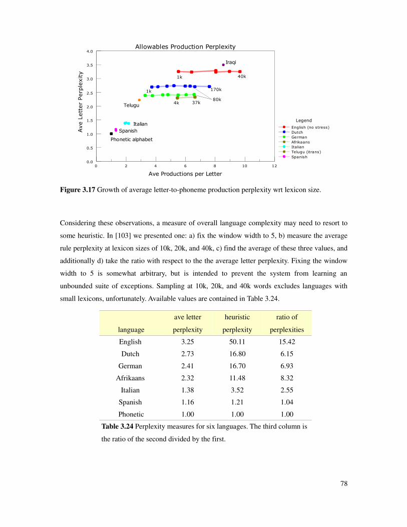
Figure 3.17 Growth of average letter-to-phoneme production perplexity wrt lexicon size.

Considering these observations, a measure of overall language complexity may need to resort to

some heuristic. In [103] we presented one: a) fix the window width to 5, b) measure the average

rule perplexity at lexicon sizes of 10k, 20k, and 40k, c) find the average of these three values, and

additionally d) take the ratio with respect to the the average letter perplexity. Fixing the window

width to 5 is somewhat arbitrary, but is intended to prevent the system from learning an

unbounded suite of exceptions. Sampling at 10k, 20k, and 40k words excludes languages with

small lexicons, unfortunately. Available values are contained in Table 3.24.

language

ave letter

perplexity

heuristic

perplexity

ratio of

perplexities

English 3.25 50.11 15.42

Dutch 2.73 16.80 6.15

German 2.41 16.70 6.93

Afrikaans 2.32 11.48 8.32

Italian 1.38 3.52 2.55

Spanish 1.16 1.21 1.04

Phonetic 1.00 1.00 1.00

Table 3.24 Perplexity measures for six languages. The third column is

the ratio of the second divided by the first.

78

Legend

English (no stress)

Dutch

German

Afrikaans

Italian

Telugu (itrans)

Spanish

37k4k

170k1k

Ave Productions per Letter

0 2 4 6 8 10 12

Ave Letter Perplexity

0.0

0.5

1.0

1.5

2.0

2.5

3.0

3.5

4.0Allowables Production Perplexity

Spanish

Iraqi

Phonetic alphabet

1k 40k

80k

Telugu

Italian

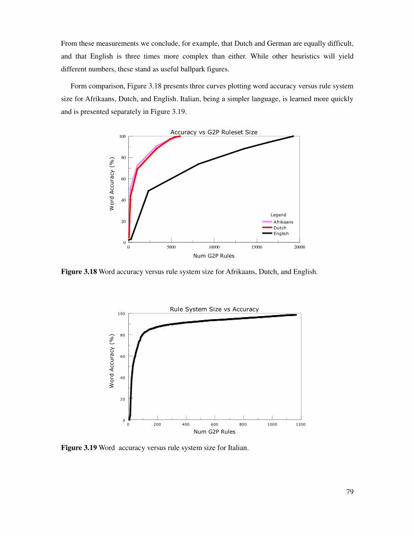
From these measurements we conclude, for example, that Dutch and German are equally difficult,

and that English is three times more complex than either. While other heuristics will yield

different numbers, these stand as useful ballpark figures.

Form comparison, Figure 3.18 presents three curves plotting word accuracy versus rule system

size for Afrikaans, Dutch, and English. Italian, being a simpler language, is learned more quickly

and is presented separately in Figure 3.19.

Figure 3.18 Word accuracy versus rule system size for Afrikaans, Dutch, and English.

Figure 3.19 Word accuracy versus rule system size for Italian.

79

Num G2P Rules

0 200 400 600 800 1000 1200

Word Accuracy (%)

0

20

40

60

80

100Rule System Size vs Accuracy

Num G2P Rules

0 5000 10000 15000 20000

Word Accuracy (%)

0

20

40

60

80

100Accuracy vs G2P Ruleset Size

Legend

Afrikaans

Dutch

English

Figure 3.20 Word accuracy versus lexicon size for Spanish, English, Italian, Afrikaans, German,

and Iraqi Arabic. The ten thousand dictionary words of English having the highest G2P regularity

lies between Spanish and Italian in complexity.

80

Lexicon size (words)

1 10 100 1000 10000 100000

Accuracy (%)

0

20

40

60

80

100Language G2P Accuracy

Legend

Spanish

English regular 10k

Italian

Afrikaans

German

English no stress

English with stress

Iraqi Arabic

3.4 Active learning and word ordering

The representation of linear rule chains has the benefit of easily fitting the needs of incremental

learning. Because rule chains ban be efficiently updated one word at a time, the learner can

operate in an interactive system with incrementally improving predictive ability. With the user

and system operating in a collaborative manner: can the system choose words an ordering of

words that optimizes performance? If the word list has thousands or tens of thousands of entries,

and the user can only invest a few hours of time, what is the most effective use of the user's time

and knowledge? This section investigates the effect of word ordering on rule learning.

Active learners [79][133] are the class of learning algorithms that not only infer a mapping

function from training data, but also controls the order in which it is exposed to training samples.

If the domain is a continuous space in ℝn the active learner can freely sample this space. In the

G2P application the domain is the discrete vocabulary provided to the system, where sampling is

a matter of picking words from the list. Words may be sampled with or without replacement. The

default behavior is that once a word is presented to the user for pronunciation information it is

considered done and put on the finished stack. However, human beings are fallible. It is possible

for an active learner to revisit a word if a) it has a measure for judging confidence, and b) it

considers the word's pronunciation to be questionable and in need of a double-check.

Optimization involves several aspects [129]. One is that not all requests for information are

equally easy for the human to provide. Long words are almost invariably more difficult than short

words. Another is that some words are more valuable than others, due to greater token occurrence

in the text corpus. A third issue is how quickly a certain sequence of words supports learning of

the G2P rules. To concoct a counterexample: suppose the sampling algorithm begins with the

word “a” and continues with “ab” “abba” “ba” “bab,” and then “bac” “ca” “cab” and so forth in

this alphabetical fashion. With respect to the final set of G2P rules, that is an unnecessarily

redundant sequence; 90% of the lexicon will pass by before anything is learned of 'y' and 'z'.

With an active learner in control and seeking to improve its knowledge, each additional word

sampled should maximize the marginal information gain. Two barriers stand in the way. First, the

final rule system is not known in advance. It only knows its history and current form. Second,

when the learning initiates the production probabilities are imprecise, resulting in poor alignment

between the graphemes and phoneme strings. Thus, while the next word might provide new rule

information, the learning may not be able to properly make use of it. An ideal active learner,

therefore, should possess an element of self-awareness.

81

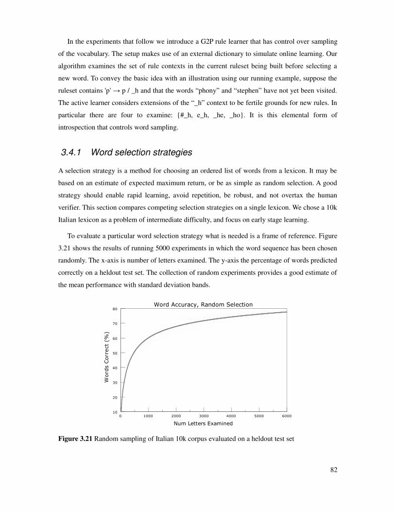
In the experiments that follow we introduce a G2P rule learner that has control over sampling

of the vocabulary. The setup makes use of an external dictionary to simulate online learning. Our

algorithm examines the set of rule contexts in the current ruleset being built before selecting a

new word. To convey the basic idea with an illustration using our running example, suppose the

ruleset contains 'p' → p / _h and that the words “phony” and “stephen” have not yet been visited.

The active learner considers extensions of the “_h” context to be fertile grounds for new rules. In

particular there are four to examine: #_h, e_h, _he, _ho. It is this elemental form of

introspection that controls word sampling.

3.4.1 Word selection strategies

A selection strategy is a method for choosing an ordered list of words from a lexicon. It may be

based on an estimate of expected maximum return, or be as simple as random selection. A good

strategy should enable rapid learning, avoid repetition, be robust, and not overtax the human

verifier. This section compares competing selection strategies on a single lexicon. We chose a 10k

Italian lexicon as a problem of intermediate difficulty, and focus on early stage learning.

To evaluate a particular word selection strategy what is needed is a frame of reference. Figure

3.21 shows the results of running 5000 experiments in which the word sequence has been chosen

randomly. The x-axis is number of letters examined. The y-axis the percentage of words predicted

correctly on a heldout test set. The collection of random experiments provides a good estimate of

the mean performance with standard deviation bands.

Figure 3.21 Random sampling of Italian 10k corpus evaluated on a heldout test set

82

Num Letters Examined

0 1000 2000 3000 4000 5000 6000

Words Correct (%

)

10

20

30

40

50

60

70

80Word Accuracy, Random Selection

Against this frame of reference we can compare four simple strategies.

alphabetical word ordering

reverse alphabetical word ordering

words ordered by increasing length, then alphabetically within the groups of equal length

words

greedy n-gram coverage

To explain word selection based on n-gram coverage, let g i ,n=c1 c2cn be an n-gram of n

characters. Let Gw ,n=g i ,n w be all the n-grams of length n in a word w. These sets of n-grams

are ordered by increasing length.

Gw=g i ,1, g i , 2 ,g i ,n,w ordered n-grams of w (3.47)

Let V be the vocabulary of words so far seen by the active learner and define Gw + to be the set

of unseen n-grams present in word w.

V =w1, w2, w3 visited words (3.48)

GV=g i ,1, g i , 2, g i , n , V visited n-grams (3.49)

Gw +=g i ,1w−g i , 1V , g i , 2w−g i , 2V ,

=g i ,1w + , g i , 2w + , unseen n-grams of w (3.50)

Score w=∑i

countg i ,1w + , score of word w (3.51)

wbest=argmaxw Score w w∈Lexicon−V best word (3.52)

The score for a word is an ordered tuple of the number of unseen unigrams, unseen bigrams,

unseen trigrams, and so on. Each n-gram is weighted by the total number of occurrences of the n-

gram in the corpus. Words are ranked first by the unigram score, then by the bigram score in the

case of a tie, etc. A greedy n-gram search therefore seeks complete unigram coverage, before

covering bigrams and trigrams and longer units if it comes to that.

In Figure 3.22 the performance of these four selection strategies is compared to average

random performance. Of the first three, reverse alphabetical performs best because it introduces a

greater variety of n-grams more quickly than the others. Yet, all of these three are substantially

worse than random. Notice that grouping words from short to long degrades performance. Since

it is easier for humans to assess shorter words than longer, this suggests that strategies tuned to

the needs of human users will incur a machine learning penalty.

83

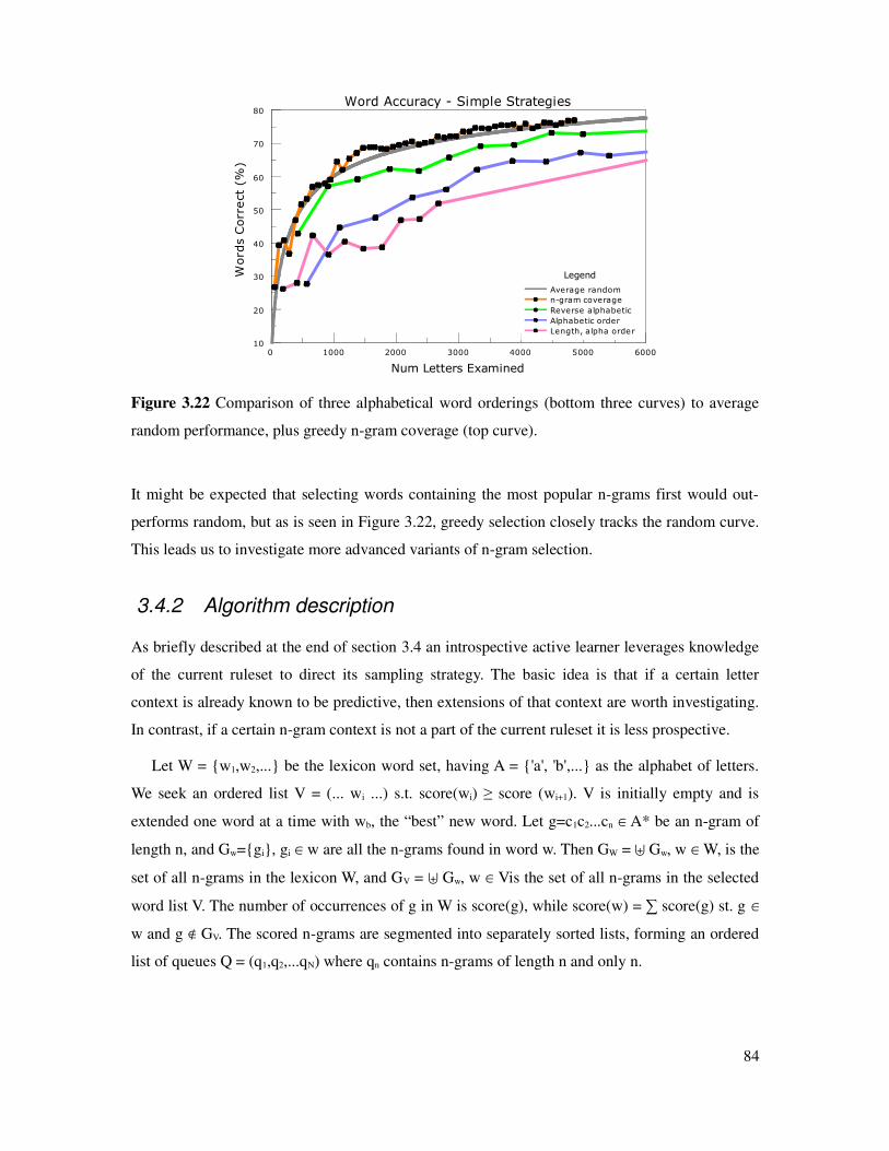
Figure 3.22 Comparison of three alphabetical word orderings (bottom three curves) to average

random performance, plus greedy n-gram coverage (top curve).

It might be expected that selecting words containing the most popular n-grams first would out-

performs random, but as is seen in Figure 3.22, greedy selection closely tracks the random curve.

This leads us to investigate more advanced variants of n-gram selection.

3.4.2 Algorithm description

As briefly described at the end of section 3.4 an introspective active learner leverages knowledge

of the current ruleset to direct its sampling strategy. The basic idea is that if a certain letter

context is already known to be predictive, then extensions of that context are worth investigating.

In contrast, if a certain n-gram context is not a part of the current ruleset it is less prospective.

Let W = w1,w2,... be the lexicon word set, having A = 'a', 'b',... as the alphabet of letters.

We seek an ordered list V = (... wi ...) s.t. score(wi) ≥ score (wi+1). V is initially empty and is

extended one word at a time with wb, the “best” new word. Let g=c1c2...cn A* be an n-gram of

length n, and Gw=gi, gi w are all the n-grams found in word w. Then GW = 5 Gw, w W, is the

set of all n-grams in the lexicon W, and GV = 5 Gw, w Vis the set of all n-grams in the selected

word list V. The number of occurrences of g in W is score(g), while score(w) = ∑ score(g) st. g

w and g v GV. The scored n-grams are segmented into separately sorted lists, forming an ordered

list of queues Q = (q1,q2,...qN) where qn contains n-grams of length n and only n.

84

Num Letters Examined

0 1000 2000 3000 4000 5000 6000

Words Correct (%

)

10

20

30

40

50

60

70

80Word Accuracy - Simple Strategies

Legend

Average random

n-gram coverage

Reverse alphabetic

Alphabetic order

Length, alpha order

Algorithm

for q in Q

g = pop(q)

for L = 1 to |longest word in W|

Wg,L = wi s.t. |wi| = L, g wi and wi∉V

wb = argmax score(Wg,L)

if score (wb) > 0 then

V = V + wb

GV = GV U Gwb

return wb

In this search the outer loop orders n-grams by length, while the inner loop orders words by

length. For selection based on n-gram coverage, the queue Q is computed only once for the given

lexicon W. In our active learner, Q is re-evaluated after each word is selected, based on the n-

grams present in the current G2P rule contexts. Let GG2P = gi s.t. gi some letter context in the

G2P rules. Initially GG2P,0 = . Then, at any iteration k, GG2P,k are the n-grams present in the rules,

and G'G2P,k+1 is an expanded set of candidate n-grams that constitute the elements of Q. G' is

formed by prepending each letter c of A to each g in G, plus appending each c to g. That is,

G'G2P,k+1 = A%GG2P,k 4 GG2P,k%A where % is the Cartesian product. Executing the algorithm returns

wb and yields GG2P,k+1 the set of n-grams covered by the expanded rule set. In this way knowledge

of the current G2P rules guides the search for maximally informative new words.

3.4.3 Active learner performance

Figure 3.23 displays the performance of our active learner on the Italian 10k corpus. For the first

50 characters encountered it under-performs average random. For the range of 50-500 characters

the active learner's performance is almost everywhere better than average random, typically one

half to one standard deviation above this reference level. Beyond 500 characters the curve tightly

tracks average random. The sobering conclusion, that cannot be avoided, is that random word

selection is hard to beat.

85

Figure 3.23 From top to bottom: a perfect Oracle, a word selection Oracle, our active learner, and

average random performance. The perfect Oracle demarcates an impossibly high optimal

performance, while Oracle word selection suggests near-optimality. Standard deviation error bars

are added to the random curve.

Two other references are shown. Immediately above the active learner curve is “Oracle” word

selection. The Oracle has access to the final G2P system and selects words that maximally

increases coverage of the known rules. The topmost curve is for a “Perfect Oracle.” This

represents an even more unrealistic situation in which each letter of each word carries with it

information about the corresponding production rule. For example, that 'g' → f / _h 10% of the

time (as in “laugh”) while 'h' → sil / g_ (“northgate”). Carrying complete information with each

letter allows the G2P system to be constructed directly and without mistake. In contrast, the non-

perfect oracle makes mistakes sequencing rules in each letter's rule chain. This decreases

performance.

In the 50-500 character range, the active learning algorithm straddles the zone in between

average random (the baseline) and Oracle word selection (near-optimality). Less favorable is the

non-monotonicity of the performance curve; for example, when the number of letters examined is

135, and 210. Analysis shows that these drops occur when a new G2P production is encountered

but more than one context offers an equally likely explanation. Faced with a tie, the G2P learner

sometimes chooses incorrectly. Not being aware of this mistake it does not seek out correcting

words. Flat plateaus occur when additional words (containing the next most popular n-grams) do

not contain previously unseen letter-to-sound productions.

86

Legend

Perfect Oracle

Oracle word selection

Active learner

Averge random

Num Letters Examined

0 100 200 300 400 500

Words Correct (%

)

0

20

40

60

80

100Word Accuracy - Active Learner

3.4.3.1 Why active learning is inherently limited

The word selection experiments of this section indicate that as a method, random selection is hard

to outperform. The same behavior has been reported with regards to optimal prompt selection for

training ASR [79] and building general purpose TTS voices [107]. What can explain this?

Observe that words are chosen based on the desire for information about a particular n-gram

that is presumed to be highly informative. But the n-gram sought is carried in a word that, of

course, contains many more n-grams. On average, the “extra cargo” will approach the same

n-gram distribution as the larger population in whole. Thus the word selection strategies with a

targeted goal will, on balance, present just small perturbations away form random. As the number

of words selected increases, the two curves converge.

Separating out the influence of extra-cargo n-grams requires a more fine grained experimental

setup. Rather than words, individual n-grams would need to be he atomic elements of learning.

Only when n-gram/phoneme pairs are sampled independently and incrementally, can the

advantage of optional selection be expected to outperform the alternative. However, in a realistic

evaluation it is expected that the learner determine the G2P alignment without external assistance.

Therefore, while a fine-grained experiment that demonstrates a clear advantage for active

learning may be of theoretical interest, it is unlikely to translate into practical consequence.

3.4.4 Token weighted word selection

The motivation behind active learning is to find a word sequence that optimized the rate at which

G2P rules are learned. The idea is that if this happens quickly then the effort required of the

person developing the lexicon is lessened. Yet, this criteria is only indirectly related to the

efficiency of creating a speech synthesizer. Instead words can be selected based on how common

they are. This is a more application-centric optimization.

A selection strategy based on word frequency requires a corpus of text from which to estimate

probabilities. We assume that this is available in two forms. First, as a large corpus of text in the

target language (with words whitespace separated). And second, as a smaller prompt list of

recorded utterances. Both cannot be optimized simultaneously. The argument for selecting words

in corpus-based frequency is that this provides the fastest way of covering the application's

intended usage. The argument for selecting words in prompt-based frequency is that since the

synthesizer is constructed from the prompt wavefiles themselves, these transcripts should be as

accurate as possible.

87

The following two figures illustrates the growth rate in token coverage of a small English

application. The coverage is measured for a) the prompt list (Figure 3.24), and b) the larger text

corpus (Figure 3.25). Three selection strategies are compared.

1. cover the prompts first by word frequency, then the corpus

2. cover the corpus first by word frequency, then the prompts.

3. interleave words from the above two strategies.

In the applications described later in Chapter 5, the first strategy was employed.

Figure 3.24 Coverage of prompt list tokens under three selection strategies.

Figure 3.25 Coverage of corpus tokens under three selection strategies.

88

Word Num

0 500 1000 1500 2000

Percent coverage

25

50

75

100Corpus Token Coverage

Legend

prompts then corpus

alternating selection

corpus then prompts

Word Count

0 500 1000 1500 2000

Percent coverage

25

50

75

100

Prompt Token Coverage

Legend

prompts then corpus

alternating selection

corpus then prompts

3.5 Connection to rest of thesis

In this chapter we have developed a grapheme-to-phoneme rule learner that will take advantage

of, but can operate without the need for human-seeded constraints. We have contrasted machine-

learned rules with rules hand-written by human experts. We have presented a formal description

of G2P rules, shown the connection to CART tree learning, and contrasted the two. Also

addressed is the issue of multiple pronunciation prediction and the assignment of probabilities.

Further, we have investigated word ordering from three perspectives. One is the issue of

ordering words to optimally support the G2P alignment problem. We presented a cell visitation

strategy based on a minimal-length-mismatch heuristic. The second perspective is the question of

ordering words to optimize the rule learning rate. We compared random selection to a range of

deterministic algorithms including an active learner that leverages knowledge of the current rules

structure. Our experiments demonstrated that random selection establishes a difficult-to-

outperform baseline, and we offered a plausible explanations for this. And third, we briefly

discussed word ordering from the perspective of prompt and corpus token coverage.

With this knowledge at our disposal, it is enlightening to take the tools out of the lab and

examine how real users engage the process of lexicon creation and review. Fields studies will

provide information on what realistic applications embody, what problems users encounter,

typical patterns of behavior, and how much time is devoted to the task. This is the subject of the

next chapter.

89

90

4 Field Studies

This chapter describes lexicon development in an existing bilingual, bidirectional speech-to-

speech translation system. Lexicon development includes the two tasks of verifying existing

entries and in adding new entries. The speech-to-speech system is the Carnegie Mellon

implementation of the TransTac Project portable translation device [11]. The device is a hand-

held or laptop that provides interactive machine translation between English and colloquially

spoken Iraqi Arabic. Targeted domains include checkpoint control, disaster relief with basic

medical services, and city infrastructure evaluation (e.g. sewer repair and refuse collection). In a

disaster relief situation, doctors, paramedics, and relief workers need to ask questions such as

“When did you last eat?” and “Where does it hurt?”. At a military checkpoint the device is

expected to translate into Iraqi Arabic questions such as “Is this your truck?” or “What is your

destination?”, and to translate back the subject's response. The lexicon must support and be tuned

towards the commonly used language of the intended particular domain.

The TransTac project has undergone several formal evaluations, typically held according to a

semi-annual schedule. The work described in this chapter was performed in preparation for the

June 2008 and November 2008 evaluations. For the June 2008 evaluation the organizers

established the specific goal of evaluating “named entity” capability (in addition to the basic

components and overall system performance). Named entities are Iraqi proper nouns: person

names, tribe names, city and street names, etc. Support for named entities is necessary so that the

Iraqi ASR component can recognize the subject's answers to questions such as “Where are you

coming from?” and then synthesize the answer to the English-speaking interlocutor. Prior to the

June 2008 evaluation the TransTac organizers provided a specific list of over 8000 named entities

to be accommodated, with a portion heldout for testing. This list of words was accompanied with

suggested pronunciations, but these were not human-verified. (The Named Entity word list is

91

described in greater detail in section 4.2.2.) We provided a tool for native speakers to verify and

correct the pronunciations.

If the G2P rule system of Arabic were straightforward and predictable, the injection of new

vocabulary would present little problem. As revealed last chapter, Arabic has an extremely

complex G2P system. Figure 3.20 of Chapter 3 shows Iraqi Arabic to be the most difficult

language of our suite of test languages; notably, it is the only language more irregular than

English. This degree of irregularity makes it highly desirable to have native speakers verify

predicted pronunciations for a) the new Named Entity word list, and b) the existing general

purpose dictionary. To assist with the CMU effort, two native speakers of Iraqi Arabic provided

lexicon review using our tool. Each is a native speaker of Iraqi Arabic (southern dialect), are well

educated, fluent in English, versed in Modern Standard Arabic, but are not linguists. Not being

linguists, they were not familiar with the formal concept of phonemes or the IPA alphabet.

Naturally they possess a speaker's understanding of pronunciation, and of the relationship

between spelling and pronunciation as taught in school and accumulated with experience.

The purpose of this chapter is to illustrate the practical nature of lexicon development within

an existing system, and to show how the techniques developed in chapter 3 are applied to a

language that is especially challenging. The TransTac system is targeted towards serious real-

world field use and is evaluated by reviewers closely affiliated with the target users, i.e. deployed

military personnel. Sections 4.2 and 4.3 describe the available lexical resources and the tasks

undertaken. To better explain the difficulties addressed, section 4.4 elaborates on Arabic writing

and phonology.

Of interest to project managers is the level of productivity can be expected from non-linguist

natives speakers; in particular, the number of words reviewed per hour. Section 4.5 quantifies the

human usage of our lexicon verification application. In addition to measuring human efficiencies,

one can also examine patterns of application usage. An unexpected finding was that one of the

users operated according to two distinct modes of operation, depending – we hypothesize – on the

level of confidence the user had in the primary pronunciation. Details and discussion are found in

section 4.5.4 .

In the time available for the June 2008 evaluation, the native speakers reviewed 1000 words of

the Named Entity list for use by the English TTS component. The span of time to the November

2008 evaluation allowed for more extensive human verification.

Finally, we draw some observations about how to increase the efficiency of lexical work, and

92

how it may be incorporated into the topic integrated voice bootstrapping discussed in the next

chapter.

4.1 Speech-to-Speech System Description

Figure 4.1 Generic high-level architecture of a speech-to-speech system. In the CMU system

Iraqi text is handled in standard, or unvowelized form.

The high-level architecture of a speech-to-speech system is commonly depicted as in the figure

above. The arrows indicate a single dialog turn originating from the English speaker.

Communication between a pair of humans is mediated by a dialog system exploiting two

corresponding recognizers, two synthesizers, and two text-to-text translation components. Each of

the ASR and TTS components necessarily relies on a phoneme set and lexicon. While it would be

a natural engineering choice for the components of a given language to use identical phonesets

and lexicons, this is not mandatory. For the sake of optimizing component (and overall system)

accuracy, it may not even be desirable. Since they serve different purposes, the English ASR and

TTS components are free to use differing phoneme sets. In stressed-timed languages such English

and German, for example, it is typical for the synthesizer to use a phoneset with 2-level stress

markings on the vowels, while the recognition component usually will make no such distinction.

In addition, the component lexicons may differ based on the needs of typical usage. In

TransTac, the English speaker in checkpoint situations asks questions such as “where are you

traveling?” and relatively few of the form “are you traveling to location?”. In contrast, Iraqi

speakers will more frequently say “I am going to location,” with a larger number of concrete

names substituted. Thus the English ASR and Iraqi TTS lexicons can manage without having

many named entities defined, while the Iraqi ASR and English synthesizer requires many.

Another difference is common. It is usual for the ASR lexicon to contain multiple

pronunciations of a given word, while the TTS lexicon contains only one pronunciation. While

93

English ASR Eng→Iraqi Iraqi TTS

Iraqi ASREng←IraqiEnglish TTS

MT

the TTS pronunciation usually matches the primary (i.e. most frequently occurring) ASR

pronunciation, this is not mandatory. For sake of understandability, or perhaps to emulate an

esteemed dialect, the TTS lexicon may adopt less colloquial forms. In our verification work, a

single best pronunciation was elicited according to what the native speaker consider “right” for

the local populace.

In the CMU Transtac system, the phonesets and lexicons for matching ASR/TTS components

are slightly different. Most differences are superficial, i.e. the file formats differ and the symbols

used to represent a particular phoneme are not the same. The mapping between phonesets is

almost but not completely one-to-one. Part of the reason is historical; the English ASR and TTS

components were independently developed by separate entities, before the project initiated. There

are also technological reasons. The speech recognizers are initialized during training by adapting

a GlobalPhone acoustic models to the target language [134]. This initialization procedures places

constraints on the ASR phoneset, which the TTS component need not adhere to.

Managing a set of lexicons that are defined using different phonesets presents extra

complications. It poses the question of which should be used for lexical work. We adopted the

synthesizer's phoneset as the “source representation” and the ASR phoneset as “derived.” Since

the synthesizers are employed to aid human verification, maintenance is easier to accomplish if

the pronunciation variants are written in the phoneset used to synthesize the speech samples. (see

section 4.5.1 for screenshots of the interface.) The minor differences between the two are

explained in the discussion of the Iraqi Arabic phonetic inventory, of section 4.4.2.

4.2 Provided lexical resources

We employ two provided lexical resources. The first is a general dictionary of Iraqi Arabic words

that has been annotated by native speakers. This is our reference dictionary. The second is the

Transtac Iraqi Names Collection database, or the “Named Entity” list for short. It contains proper

nouns such as place names, street names, person names, etc. This list is provided with

pronunciation hints, but as provided was not reviewed by human annotators. The reference

dictionary contains over 42 thousand word forms; the Named Entity list contains 8689 unique

words [77].

The reference lexicon is not, strictly speaking, a pronunciation dictionary. This is because it

does not define a phoneme set and does not provide phonetic transcriptions. Instead the words are

fully spelled out in “citation form”. The citation form of a word in modern standard Arabic is a

sequence of graphemes with detailed diacritical marks sufficient to provide nearly unambiguous

94

pronunciation. This extra level of detail is seldom provided in the normal written form. because

the extra information primarily pertains to vowels, this process is also called vowelization. A

detailed description of the diacritics used for citation (vowelization) is saved for section 4.4.5.

Conversion from the citation word form (or its transliteration) into phoneme strings is left to

individual project teams.

4.2.1 Reference lexicon

The reference pronunciation dictionary provided to members of the TransTac project has been

collected and distributed by the Linguistic Data Consortium (LDC, [111]). The edition used in

this work is ver5.2. It contains 42,735 word forms, and so is referred to as the “42k dictionary.”

The dictionary is derived from the transcription of 20 hours of speech data – a corpus containing

approximately 1,493,793 word tokens and 61,937 distinct word forms [77]. Roughly 17k word

forms did not make it into the version 5.2 edition.

The 42k dictionary is distributed as a tab-delimited utf-8 Unicode text format file. In parallel

with the Arabic word forms represented in utf-8, a transliteration scheme known as Buckwalter

provides a one-to-one mapping from the Unicode codepoints values into the printable ASCII

range [34]. Buckwalter has ASCII symbols for all consonants and vowels and diacritic marks. In

the text file each line consists of five fields. We illustrate with the entry “atkallam”.

أ أ >tklm >atkal~am IV1S

1. The original word in orthographic form, as found in the transcripts, in utf-8.

2. Reference vowelized form in utf-8, created by morphological annotation.

3. An unvowelized Buckwalter form (segmented into morphemes).

4. An vowelized Buckwalter form (segmented into morphemes).

5. Segmented parts of speech tags.

Vowelization of forms was performed (by the LDC) by having two native Iraqi speakers mark up

the words with diacritics. They used by using their linguistic knowledge for this task. This is in

contrast to earlier versions of the dictionary in which non-native speakers annotated with the aid

of the acoustic transcripts [77]. The vowelized Buckwalter form (fourth field) is a direct

transliteration of the diacriticalized utf-8 form (second field). Deleting the Buckwalter letters

corresponding to diacritics produces the third field. Details of Buckwalter transliteration are

presented below in Table 4.8 and Table 4.9. The parts of speech tags (fifth field) are the product

95

of morphological analysis performed by the native speakers, but is not relevant to lexical work.

It is important to bear in mind that writing fully diacriticalized or “citation form” Arabic is an

uncommon activity even for native speakers. There will be a degree of randomness to

vowelization. In lexicon's documentation there is no mention of inter-labeler agreement [77],

presumably because the two annotators worked on mutually exclusive sets. However a

comparison could be made to a smaller, independently produced lexicon known as the APPEN

dictionary [6]. This dictionary has 18,327 word forms, and of these 14,641 overlap with the LDC

dictionary. The overlap set contains 59.8k “decision points” – i.e. consonants. The consensus

between the two dictionaries is 77.3% (46.2k consonants) and 29.4% at the word level (4.3k /

14.6k). The single largest source of discrepancy involved one dictionary adding a diacritic while

the other left the consonant unmarked. At this rate, the LDC dictionary may have about 25%

vowel annotations susceptible to minor discrepancy.

4.2.2 Transtac Iraqi Names Collection database

The second provided lexical resource is the Transtac Iraqi Names Collection speech database. The

speech component of this data set consists of 250 native speakers of one recording session each.

A session had the speaker reading supplied scripts of names, and then devising a sentence of their

own making containing the name. To generate additional entries not anticipated by the data

collectors, speakers were also asked to spontaneously create both the names and the sentences.

Within each session speakers were asked to say names from a set of ten categories, listed in the

following table. These are Iraqi male first names, Iraqi female names, Iraqi surnames, Iraqi tribe

names, non-Iraqi male first names, non-Iraqi tribe names, place names, street names, entity names

(such as businesses, hospitals, schools, governments, etc.), and titles (such as Mr., Mrs., Dr. etc.).

The Named Entity is a distributed as a 7-column tab-separated file. Words may have multiple

entries when alternate transliterations are provided. The first five fields are relevant.

1. The name written in undiacriticized Arabic.

2. A vowelized transliteration of the name in Buckwalter form.

3. A transliteration of the name into English-like spelling.

4. A ranking of the word when multiple transliterations are provided.

5. A translation of the name when available.

96

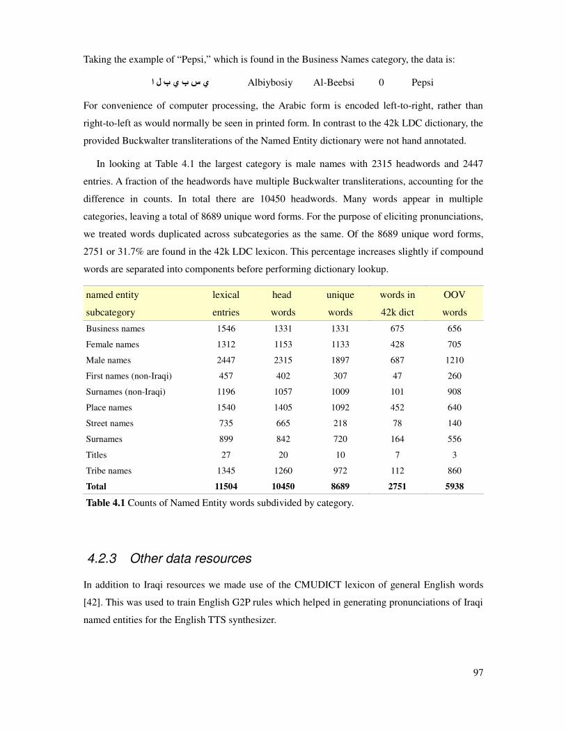
Taking the example of “Pepsi,” which is found in the Business Names category, the data is:

ي س ب ي ب ل ا Albiybosiy Al-Beebsi 0 Pepsi

For convenience of computer processing, the Arabic form is encoded left-to-right, rather than

right-to-left as would normally be seen in printed form. In contrast to the 42k LDC dictionary, the

provided Buckwalter transliterations of the Named Entity dictionary were not hand annotated.

In looking at Table 4.1 the largest category is male names with 2315 headwords and 2447

entries. A fraction of the headwords have multiple Buckwalter transliterations, accounting for the

difference in counts. In total there are 10450 headwords. Many words appear in multiple

categories, leaving a total of 8689 unique word forms. For the purpose of eliciting pronunciations,

we treated words duplicated across subcategories as the same. Of the 8689 unique word forms,

2751 or 31.7% are found in the 42k LDC lexicon. This percentage increases slightly if compound

words are separated into components before performing dictionary lookup.

named entity

subcategory

lexical

entries

head

words

unique

words

words in

42k dict

OOV

words

Business names 1546 1331 1331 675 656

Female names 1312 1153 1133 428 705

Male names 2447 2315 1897 687 1210

First names (non-Iraqi) 457 402 307 47 260

Surnames (non-Iraqi) 1196 1057 1009 101 908

Place names 1540 1405 1092 452 640

Street names 735 665 218 78 140

Surnames 899 842 720 164 556

Titles 27 20 10 7 3

Tribe names 1345 1260 972 112 860

Total 11504 10450 8689 2751 5938

Table 4.1 Counts of Named Entity words subdivided by category.

4.2.3 Other data resources

In addition to Iraqi resources we made use of the CMUDICT lexicon of general English words

[42]. This was used to train English G2P rules which helped in generating pronunciations of Iraqi

named entities for the English TTS synthesizer.

97

4.3 Task descriptions

In the CMU Transtac system, lexicon maintenance involves four distinct phonesets and lexicons.

However, as mentioned earlier, the usage of named entity words is asymmetrical. Adding these

words to the system impact only the Iraqi Arabic ASR and the English TTS components. The

English ASR lexicon is considered stable. The large general-purpose Iraqi lexicon (prior to the

addition of named entities) is considered adequate, but open to improvement.

Five specific lexicon maintenance tasks are defined, listed in approximate order of priority.

1. English TTS NE. Enhance the English TTS lexicon with English-accented versions

of Iraqi named entity words. The English synthesizer is used to assist the human verifier.

The goal is a synthesizer that speaks Iraqi proper nouns as correctly as possible.

2. Iraqi ASR NE. Enhance the Iraqi Arabic ASR lexicon with the Iraqi named entity

words. The Iraqi synthesizer is used to assist the human verifier. The goal is a larger

recognition vocabulary with reduced word error rates.

3. Iraqi-English G2P Rules. Using the results of tasks 1 and 2, train an Iraqi-to-English

G2P rule system. The benefit is the ability for the English synthesizer to pronounce Iraqi

words passed through in Arabic script. This happens when the Iraqi-English MT

subsystem encounters an out-of-vocabulary word from the Iraqi recognizer (as can

occasional happen), and passes it through unchanged.

4. Iraqi-English P2P Rules. Using the results of the above two tasks, train a phoneme-

to-phoneme mapping between the two language. The goal is to replace a hand-created

cross-lingual phoneset mapping with an improvement based on native speaker

information.

5. Iraqi ASR/TTS general lexicon. Verify and/or improve the existing general Iraqi

lexicon, i.e. the common non-named entity words. This larger goal is outside the context

of the current work.

An advantage of the TransTac project is that the English and Iraqi unit-selection synthesizer were

developed by a commercial entity specifically for this project, and are consequently of high

quality [37]. In a pre-test with our native speaker, we played examples of isolated words produced

by these synthesizers, inquiring if variations in pronunciation were understandable and

distinguishable. The answer was affirmative. With this hurdle crossed, our fundamental strategy is

to present multiple pronunciation variants using the available resources (including G2P rule

98

prediction), to synthesize them with the existing synthesizer, and to have the native speaker

review the candidates.

The central tool used for the verification task is a customized version of our “LexLearner”

software. It has the distinguishing feature of presenting multiple pronunciation hypotheses, each

with an affiliated wavefile. The user interface of this tool is shown in Figure 4.4 of section 4.5.1.

The user is asked to select the pronunciation that is best, or “none of the above” if that is the case.

The user can type in a comment if desired. Our hypothesis is that for non-technical users, a

recognition task (selecting among variant pronunciations) is easier and faster than a correction

task (editing phoneme strings). Note also that the results of our verification procedure produce

both positive and negative data points. In selecting a presented pronunciation, the user is also

declaring that the remaining pronunciations are incorrect (or at least less than best).

4.4 Orthography, transliteration, phonetics, and vowelization

of Iraqi Arabic

Perhaps the most important fact regarding Iraqi Arabic is that it is a spoken-only language.

Technically, it is a vulgar, a colloquial variation spoken by the regional populace but without a

written tradition of its own. In contrast, Standard Arabic (also called Literary Arabic) is the

language used for literary works. Scholars distinguish two related registers: the Classical Arabic

of the Koran and early Islamic literate, and the derived Modern Standard Arabic (MSA) in use

today. MSA is the literary standard across the Middle East and North Africa, and is one of the

official six languages of the United nations [121]. Most printed matter – including most books,

newspapers, magazines, official documents, even graffiti – is written in Modern Standard Arabic.

For the TransTac project, Modern Standard Arabic script was adopted to transcribe speech data

into written form, and when requested to apply MSA diacritic marks to clarify pronunciation. The

result is that the native Iraqi speakers who produced the LDC lexicon had to be trained to use

Literary Arabic (MSA) for transcribing a language not normally written. In section 4.4 we

elaborate on the relation between the phoneme inventory and the writing system of Modern

Standard Arabic that is used to transcribe Iraqi Arabic. This is important for understanding why

the text form as normally written is ambiguous with respect to pronunciation.

99

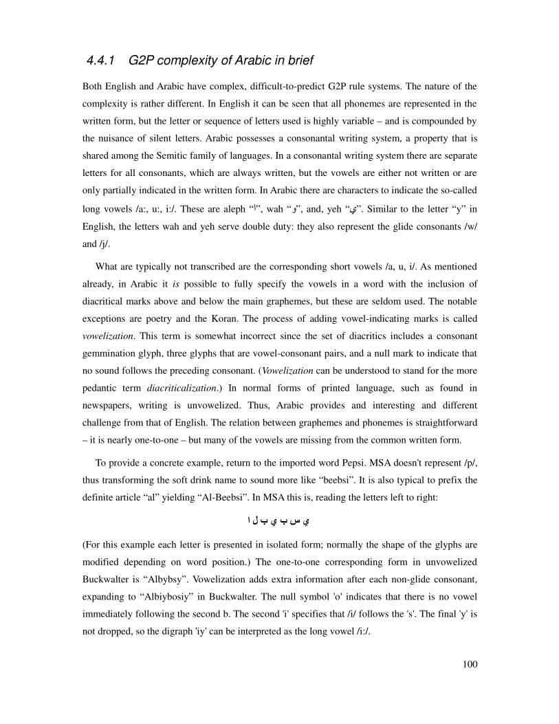
4.4.1 G2P complexity of Arabic in brief

Both English and Arabic have complex, difficult-to-predict G2P rule systems. The nature of the

complexity is rather different. In English it can be seen that all phonemes are represented in the

written form, but the letter or sequence of letters used is highly variable – and is compounded by

the nuisance of silent letters. Arabic possesses a consonantal writing system, a property that is

shared among the Semitic family of languages. In a consonantal writing system there are separate

letters for all consonants, which are always written, but the vowels are either not written or are

only partially indicated in the written form. In Arabic there are characters to indicate the so-called

long vowels /a:, u:, i:/. These are aleph “ا”, wah “و”, and, yeh “ي”. Similar to the letter “y” in

English, the letters wah and yeh serve double duty: they also represent the glide consonants /w/

and /j/.

What are typically not transcribed are the corresponding short vowels /a, u, i/. As mentioned

already, in Arabic it is possible to fully specify the vowels in a word with the inclusion of

diacritical marks above and below the main graphemes, but these are seldom used. The notable

exceptions are poetry and the Koran. The process of adding vowel-indicating marks is called

vowelization. This term is somewhat incorrect since the set of diacritics includes a consonant

gemmination glyph, three glyphs that are vowel-consonant pairs, and a null mark to indicate that

no sound follows the preceding consonant. (Vowelization can be understood to stand for the more

pedantic term diacriticalization.) In normal forms of printed language, such as found in

newspapers, writing is unvowelized. Thus, Arabic provides and interesting and different

challenge from that of English. The relation between graphemes and phonemes is straightforward

– it is nearly one-to-one – but many of the vowels are missing from the common written form.

To provide a concrete example, return to the imported word Pepsi. MSA doesn't represent /p/,

thus transforming the soft drink name to sound more like “beebsi”. It is also typical to prefix the

definite article “al” yielding “Al-Beebsi”. In MSA this is, reading the letters left to right:

ي س ب ي ب ل ا

(For this example each letter is presented in isolated form; normally the shape of the glyphs are

modified depending on word position.) The one-to-one corresponding form in unvowelized

Buckwalter is “Albybsy”. Vowelization adds extra information after each non-glide consonant,

expanding to “Albiybosiy” in Buckwalter. The null symbol 'o' indicates that there is no vowel

immediately following the second b. The second 'i' specifies that /i/ follows the 's'. The final 'y' is

not dropped, so the digraph 'iy' can be interpreted as the long vowel /i:/.

100

4.4.2 Iraqi Arabic phoneme inventory and phonology

In an encyclopedic entry such as Comrie [43], a total of 28 consonantal segments are cited for

Arabic as being “fairly typical of educated speakers.” These are presented in Table 4.2 using the

IPA consonantal chart for organization. The approximants /l, j, w/ will be familiar to English

speakers, as will the labial, dental, and plain alveolar consonants (though the trill /r/ is peculiar to

Scottish English). The remainder, except for /k/ and /h/, are not present in American English, and

provide Arabic with its distinctively “harsh” quality. Four of the alveolar consonants /t, d, s, z/

exist in contrast to their so-called “emphatic” partner. This contrast is usually described as the

effect of pronouncing the consonants as velarized or pharyngealized. Despite the term emphatic,

it is not a matter of speaking the phoneme with increased power or stress. In IPA nomenclature,

Arabic emphasis is indicated by placing the voiced pharyngeal fricative symbol ¿ in superscript

following one of /t, d, s, z/. However, it may be prudent to accept this explanation guardedly. As

Kaye writes:

The 'emphatic' consonants [are] often misleadingly called velarised-pharyngealised. ...

Perhaps nowhere else in Arabic linguistic literature is there more controversy and more

debate than in this area of the emphatics and how they are to be described and how they

function. The vowels around an emphatic consonant tend to become lower, retracted or

more centralised than around corresponding non-emphatics. [96]

In section 4.4.4 we will present spectral evidence that Kaye is correct regarding the effect on

neighboring vowels, while still suggesting that “velarised-pharyngealised” is appropriate

terminology.

In the consonant inventory below, three boxes in Table 4.2 are shaded. These identify the

locations of the labial /p/, the velar /g/, and the voiceless palatal affricative /tß/, which are three

extra elements included in the TTS phoneset. The extra three are incorporated from Persian, and

are present to support loan words into Iraqi Arabic.

101

labial dental

alveolar

palatal velar uvular pharyn glottalplain emph

nasal m n

stop voiceless t t¿ k q ÷

voiced b d d¿

fricative voiceless f ü s s¿ ß x ˛ h

voiced ∂ z ∂¿ © ¿

affricative voiceless

voiced dΩ

trill r

approximants l j w

Table 4.2 Arabic consonant inventory. The shaded boxes indicate locations of additional

phonemes present in the synthesizer's phoneset.

Table Table 4.10 on page 103 presents the ASCII representation used by the TTS and ASR

phonesets. In each location the TTS symbol is on the left and the ASR symbol is on the right.

Except for the three extra phones defined for the synthesizer, the mapping between the two

components is one-to-one. It's worth recalling that the ASR phoneme names are not arbitrary –

due to the way the recognizer initializes acoustic models, the symbols must denote a member

within the multilingual GlobalPhone inventory [136]. The symbols used by the synthesizer have

no external reference and can be any convenient ASCII string.

102

labial dental

alveolar

palatal velar uvular pharyn glottalplain emph

nasal m m n n

stop voiceless p t t tq v k k qq Q q q

voiced b b d d dq D g

fricative voiceless f f th T s s sq p sh S x x hq H h h

voiced dh C z z zq Z gq g xq X

affricative voiceless ch

voiced jh J

trill r r

approximants l l j j w

Table 4.3 Iraqi Arabic consonant phoneset used in the CMU Transtac system. In each box the

left character is the symbol used by the TTS subsystem, while the right symbol is used by the

ASR subsystem. As in Table Table 4.2 the shaded boxes indicate phonemes that are included in

the TTS phoneset, used to support loan words.

labial dental

alveolar

palatal velar uvular pharyn glottalplain emph

nasal 504 271

stop voiceless 0 305 238 227 311 0

voiced 512 658 89 0

fricative voiceless 243 57 186 199 138 127 73 82

voiced 100 166 80 72 28

affricative voiceless 1

voiced 233

trill 641

approximants 1067 2236 658

Table 4.4 Occurrence counts of geminated consonants per phoneme, taken from the LDC 42k

lexicon of reference pronunciations.

While the standard consonant inventory has 28 element, it may be considered to have as many as

56. This is because Arabic has the property of gemination. A geminated consonant is lengthened

compared to the non-geminated form, and is phomemic (meaning-contrastive) in Arabic. All

consonants in Arabic may be geminated, except for one, the glottal stop /÷/. The increase in

duration is a simple effect to achieve for sustainable consonants. (It is what children do when

103

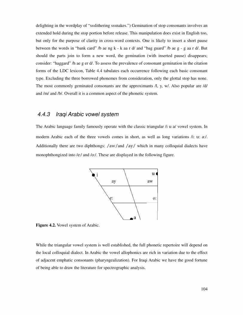
delighting in the wordplay of “ssslithering sssnakes.”) Gemination of stop consonants involves an

extended hold during the stop portion before release. This manipulation does exist in English too,

but only for the purpose of clarity in cross-word contexts. One is likely to insert a short pause

between the words in “bank card” /b ae ng k - k aa r d/ and “bag guard” /b ae g - g aa r d/. But

should the parts join to form a new word, the gemination (with inserted pause) disappears;

consider: “haggard” /h ae g er d/. To assess the prevalence of consonant gemination in the citation

forms of the LDC lexicon, Table 4.4 tabulates each occurrence following each basic consonant

type. Excluding the three borrowed phonemes from consideration, only the glottal stop has none.

The most commonly geminated consonants are the approximants /l, y, w/. Also popular are /d/

and /m/ and /b/. Overall it is a common aspect of the phonetic system.

4.4.3 Iraqi Arabic vowel system

The Arabic language family famously operate with the classic triangular /i u a/ vowel system. In

modern Arabic each of the three vowels comes in short, as well as long variations /i… u… a…/.

Additionally there are two diphthongs: /aw/and /ay/ which in many colloquial dialects have

monophthongized into /e…/ and /o…/. These are displayed in the following figure.

Figure 4.2. Vowel system of Arabic.

While the triangular vowel system is well established, the full phonetic repertoire will depend on

the local colloquial dialect. In Arabic the vowel allophonics are rich in variation due to the effect

of adjacent emphatic consonants (pharyngealization). For Iraqi Arabic we have the good fortune

of being able to draw the literature for spectrographic analysis.

104

away

e: o:

From Kaye [43]:

“the vowel allophonics have been accurately described on the basis of detailed

spectrographic analysis for the modern standard Arabic as used in Iraq. The rules may be

stated as follows:”

(1) /i…/ → [π…] / _ [+emphatic] _

→ [ˆ…] / _ ¿, © _

→ [i…] / _

(2) /i/ → [π] / _ [+emphatic] _

→ [ˆ] / _ ¿, © _

→ [i] / _

(3) /u…/ → [¨…] / _ [+emphatic] _

→ [u…]

(4) /uuuu/ → [¨] / _ [+emphatic] _

→ [u] / _

(5) /a…/ → [a…] / _ [+emphatic, q, r] _

→ [√…] / _ ¿, © _

→ [æ…] / _

(6) /aaaa/ → [\] / _# (except next to q, r, ¿, ©)

→ [a] / [+emphatic, q, r]

→ [√] / _ ¿, © _

→ [æ] / _

To summarize this list of rules, emphatic consonants act to centralize the high vowels and

preserve the lowness of /a/. Non-emphatic consonants push the vowel higher. Extra rules handle

the pairs q, r and ¿, ©. There are no allophonic rules that transform long vowels to short, or

vice versa.

This information is presented for completeness, but also to point out a limitation involved in

using a pre-build synthesizer that is not open to modification. The creators of the Iraqi Arabic

synthesizer used a six-point vowel system of /i, u, a/ in their short and long variants. The two

diphthongs were not incorporated, nor the purported allophonic variations [æ, √, ˆ, π, ¨].

105

Employing a simpler phoneset is understandable when developing a new synthesizer, particularly

when the vowel information of word is missing or ambiguous. However, it does mean that during

lexicon verification, the synthesizer may not be able to generate distinctions in sufficient

resolution to satisfy a native speaker. The tool and users must operate within these constraints.

4.4.4 Acoustic correlates of emphatic versus non-emphatic /s/

It is outside the scope of this thesis to resolve the true nature of Arabic emphatics. But since it is

such an unusual feature to a native English speaker, and since it is reportedly a matter of

longstanding dispute amongst linguists, we take a brief detour to examine utterance-initial /s/

versus /s¿/. The comparison is between two words spoken in isolation, transliterated as “safar”

(non-emphatic) and “Safar”(emphatic). Contrasting the unvoiced alveolar fricative /s/ is an

attractive choice since this phoneme can easily vary in length and intensity. The notion of

emphasis easily conjures the idea that one of these attributes (length or duration) is responsible

for the phonemic contrast. In fact, it is neither. In Figure 4.3. we see that there is no appreciable

difference in duration or intensity of the first consonant. If anything, the non-emphatic /s/ is a

slightly longer in this instance. What changes is not the qualities of the emphatic consonant itself,

per se, but the effect it has on the following vowel. Table 4.5 contains the measured values.

word phoneme

pair

following vowel

arabic translit. F1 F2

رfسس safar s a 600 1600

رfصص Safar s¿ a 700 1200

رر sAra s a… 700 1300

رر SAra s¿ a… 800 1100

Table 4.5 Measurements contrasting the formant positions of word-

initial emphatic and non-emphatics.

106

Figure 4.3. Spectrograms contrasting the effect of word-initial emphatic and non-emphatic /s/.

Images courtesy of Aaron Phillips.

Our (non-exhaustive) examination does not rule out the possibility of some contrasting feature

within the /s/ itself, but the effect is most evident on the co-articulated vowel. This can be

understood as modified articulation of the tongue dorsum. During production of the /s/, the apical

region of the tongue makes nearly the same point of contact with the palette, producing

comparable spectra. Simultaneous with this setup, the tongue dorsal reshapes backwards during

emphatic production. If this suggested mechanism is in operation, the adjustment of articulation

may legitimately be called pharyngealization. For the plain /s/ the change in vocal tract shape

results in an increase in F2, i.e. a fronting of the vowel towards [æ]. This explanation is

consistent with Kaye's rule number (5) (see above, page 105).

4.4.5 Modern Standard Arabic writing system

Modern Standard Arabic is a written language. It is a language of literature, not of the regional

spoken usage. Consequently, the majority of words present in the corpus of Iraqi Arabic

recordings simply are not part of an modern standard Arabic lexicon. This means that the

transcribers had to be trained to convert spoken words into a written form that is novel.

To appreciate the challenge of this task it is necessary to understand the ingenious nature of

morphology that exists in the Semitic family of languages, include Arabic, Aramaic and Hebrew.

Deutscher, in his popular book [62], illuminates the verbal system well.

107

safar Safar

The architecture of the Semitic verb is one of the most imposing edifices to be seen

anywhere in the world's languages, but it is founded on a concept of the sparest design: a

root which consists of only consonants. The verbal root in Semitic is not a pronounceable

chunk like English 'eat' or Latin 'ed-', but a group of just three consonants, like the Arabic

l-b-s, which means 'wear', or s-l-m, which means 'be at peace'. [62] ( pp. 36-37)

A verbal root is not a word, but exists in the service of a group of conceptually related verbs. This

is why it need not be a pronounceable sequence of phonemes. To form a word that may be used in

spoken language, the consonantal root is filled out with vowels. If we interleave the vowel pattern

a-i-a into the root s-l-m we have the second person past from ('he was at peace') s-a-l-i-m-a. In

Arabic, vowels are separated by consonants. This pattern becomes a template ,

with squares preserving slots for root consonants and circles preserving slots for vowels.

Example: s-l-m “he was at peace”

General pattern

↓ ↓ ↓

Root s l m

↓ ↓ ↓

Word template s l m

↓ ↓ ↓ ↓

Word s a l i m a

Taking the 'at peace' template and inserting another filler-pattern yields a different variant of the

root concept. Even the absence of a vowel can make a meaningful distinction. Deutscher

illustrates the possibilities by employing the imaginary root s-n-g, which, for the sake of

argument, means “to snog.”

case present past one who... the action of

simple ya s n a g u

he snogs

s a n i g a

he snogged

s a: n i g

one who snogs

s a n a: g

the action of

snogging

causative yu s n i g u

he causes to snog

a s n a g a

he caused to snog

mu s n i g

one who causes to

snog

i s n a: g

the action of causing

to snog

Table 4.6 A simplified verbal case system using the root s-n-g expanded with vowel fillers.

108

When one follows this theme with the real root s-l-m we find forms such as:

simple past salima – he was at peace

simple, action of salam – being at peace

causative, one who muslim – he was at peace

causative, action of islam – submitting to the will of God

Table 4.6 does not begin to exhaust the combinatorial possibilities, which is large. With four

vowel slots and nine values per slot (3 basic vowels in short and long, form, two diphthongs, plus

the non-productive 'vowel' epsilon) there are 94=6561 possibilities. Of course not all are used.

While Semitic morphology is impressive in its fertility, so far it presents no extraordinary

problems for letter-to-sound rules. Alas, in the interests of economy, early Semitic authors found

it sufficient to write down only the consonants, leaving it to the reader to supply the correct

missing vowels. Three graphemes do exist to transcribe the long vowels /i, u, a/, but the

graphemes are ambiguous in that they may also stand for consonants. The short vowels are not

marked. While the short vowels (and the unsounded epsilon 'vowel') do have diacritic graphemes

to indicate their presence, these are used rarely. The notable exceptions are poetry, and the Koran,

in which the religious incantations operate only if spoken exactly to the letter. The speech-to-

speech Transtac translation system is trained on transcribed texts that do not have the extra

markers disambiguating words.

Arabic is a cursive writing system. As a result the physical realization of a letter changes

depending on whether it is initial, medial, final or isolated. When represented in electronic form,

the different surface realizations receive the same underlying Unicode codepoint number. This is

unlike Latin character sets in which upper and lowercase letters stake claim to distinct codepoints.

To reduce confusion, Arabic glyphs will be displayed in their isolated form.

Arabic writing consists of baseform glyphs that are annotated with “dots and squiggles” and

which can be seen to form families. In school instruction these groups have names to aid learning.

Baseform glyphs include ح ع ر the chair group ب and the imaginatively named “duck” family ى.

Some of these related groups are collect in Table 4.7. Note that these groups of glyphs are related

in appearance only. To a native speaker they represent completely different letter sounds

109

some related character forms of Arabic

ب ن ت ث پ س ش

ح خ ج چ ص ض

ى ي ئ ط ظ

د ذ ع غ

ر ز ف ڤ

و ؤ . ة

Table 4.7 Related Arabic glyphs in no particular order. Some of these groups have

instructional names. With a bit of imagination, ى leads the “duck” group.

The Arabic characters can be divided into four sections:

1. alphabet: the base alphabet of consonants

2. vowels: the small set of written vowel

3. hamza: a set of glottal-stop/vowel pairs

4. harakat: the set of annotation diacritics.

Table 4.8 presents the base alphabet section, including the glyph in isolated form, the name of

the character, the Unicode codepoint, a transliteration into ASCII (Buckwalter), and the dominant

associated phoneme. The standalone vowels, hamza group, and harakat group are collected in

Table 4.9. The harakat group includes fatha/fathatan, damma/dammatan, and kasra/kasratan used

to insert the short vowels /a, u, i/ according to the root and filler system described in above. The

sukun symbol clarifies that no vowel follows the preceeding consonsant. Also important is the

shadda symbol, which indicates that the previous character is geminated. Diacritics such as the

hamza can convert a consonant into a vowel. For example, the wah symbol normally indicates the

high back consonant /w/, with a hamza above it marks the high back vowel /u:/ (usually word

initially, thus /÷ u:/).

110

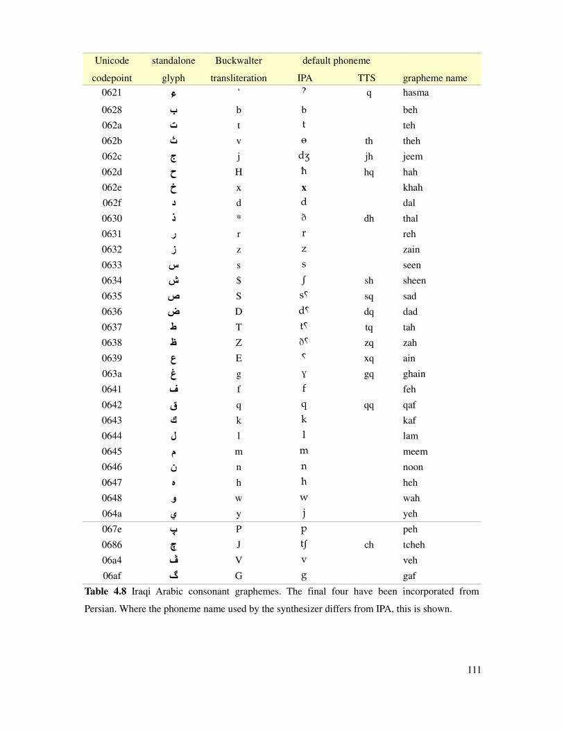
Unicode

codepoint

standalone

glyph

Buckwalter

transliteration

default phoneme

IPA TTS grapheme name

0621 ء ' ÷ q hasma

0628 ب b b beh

062a ت t t teh

062b ث v ü th theh

062c ج j dΩ jh jeem

062d ح H ˛ hq hah

062e خ x x khah

062f د d d dal

0630 ذ * ∂ dh thal

0631 ر r r reh

0632 ز z z zain

0633 س s s seen

0634 ش $ ß sh sheen

0635 ص S s¿ sq sad

0636 ض D d¿ dq dad

0637 ط T t¿ tq tah

0638 ظ Z ∂¿ zq zah

0639 ع E ¿ xq ain

063a غ g © gq ghain

0641 ف f f feh

0642 ق q q qq qaf

0643 ك k k kaf

0644 ل l l lam

0645 م m m meem

0646 ن n n noon

0647 ' h h heh

0648 و w w wah

064a ي y j yeh

067e پ P p peh

0686 چ J tß ch tcheh

06a4 ڤ V v veh

06af گ G g gaf

Table 4.8 Iraqi Arabic consonant graphemes. The final four have been incorporated from

Persian. Where the phoneme name used by the synthesizer differs from IPA, this is shown.

111

Unicode

codepoint

standalone

glyph

Buckwalter

transliteration

default

phoneme grapheme name

0627 ا A a: aleph

0648 و w u: wah (when used as a vowel)

064a ي y i: yeh (when used as a vowel)

0649 ى Y a: alef maksura

0629 ة p a teh marbuta

0671 ٱ ÷ alef wasla

0670 ` ÷ a: superscript alef

0622 1 | ÷ a: alef, madda above

0623 أ > ÷ a alef, hamza above

0624 ؤ & ÷ u: waw, hamza above

0626 ئ ÷ i: yeh, hamza above

0625 إ < ÷ i alef, hamza below

064e a a fatha

064f u u damma

0650 i i kasra

064b F a n fathatan (word final only)

064c N u n dammatan (word final only)

064d K i n kasratan (word final only)

0651 ~ geminate shadda

0652 o epsilon sukun

Table 4.9 Top section: characters that represent standalone vowels. Middle section: the

hamza/madda/wasla group that form glottal-stop/vowel pairs. Bottom section: the harakat group,

a set of diacritics used to mark consonant characters.

Despite the ambiguity introduced into the written form by the incomplete representation of

vowels, the G2P relationship for words written in citation form is nearly one-to-one. This allows

us to prepare Table 4.10 – an IPA consonantal chart with Arabic grapheme inserted. Each

character from Table 4.8 is represented.

112

labial dental

alveolar

palatal velar uvular pharyn glottalplain emph

nasal م نstop voiceless پ ت ط ك ق ء

voiced ب د ض گfricative voiceless ف ث س ص ش خ ح '

voiced ڤ ذ ز ظ غ ع affricative voiceless چ

voiced جtrill رapproximants ل ي و

Table 4.10 Iraqi Arabic consonant graphemes as they map essentially one-to-one onto the

corresponding IPA symbols. The glyphs representing palatal and velar approximants also serve

duty as vowels. Shaded squares indicate the four characters imported from Persian.

4.4.6 Grapheme to phoneme relationship

As Table 4.10 above is arranged as an IPA consonantal chart, the relationship between consonants

and phonemes is depicted as one-to-one. This much of Arabic phonology is straightforward. The

ambiguity arises with respect to the vowels. As previously explained, the writing system normally

only records the consonants in a word. Diacritic marks are critical for disambiguating

pronunciations, but are normally not written.

We may classify the action of diacritic marks as phoneme insertion, gemination, and vowel

modification. The insertion diacritics are: fatha, damma, kasra, which insert the “missing” short

vowels /a, u, i/; the parallel fathatan, dammatan, kasratan, which insert the phoneme pairs /a n,

u n, i n/. We may also include sukun (transliteration o), which indicates that no vowel sound

follows the preceding consonant – i.e. it inserts an epsilon symbol. The gemination character

shadda (transliteration ~) instructs the speaker to repeat the previous consonant or to lengthen it.

For the full set see above to Table 4.9.

113

The modification diacritics include the hamza, wasla, and madda glyphs. They modify the

vowel point /a, u, i/ and whether it is long or short. At the beginning of a word the vowel is

initiated with a glottal stop. Word-internally, this stop is elided.

Because of the template-and-fill pattern of Arabic phonology, the missing vowelization marks

are not strongly constrained by the surrounding context of written characters. There is an

irreducible amount of uncertainty. Table 4.11 illustrates this property for a selection of characters,

one character per row. The column header lists the eight possible diacritic marks, with the default

phoneme production immediately beneath. Then, in each cell is the number of occurrences of the

diacritic following the character on the left, as counted in the LDC 42k dictionary. For example, ؤ

(wah with hamza above) has a default pronunciation of /q u:/. The vowel is overridden to /a/, /i/,

and /u/ 115, 2, and 47 times respectively. From these numbers the bigram perplexity is 1.94. The

four consoants selected ('b', 'd', 'l', 'n') have a high perplexity of between 3 and 4.

Following diacritic

a i u o F K N ~

character glyph phone a i u nil an in un gem. perplex

ا a: 84 86 11 15 211 3.37

1 q a: 10 1.0

أ q a 3702 165 233 2 1.47

ؤ q u: 115 2 47 1.94

إ q i 37 1930 1.10

ئ q I 76 485 3 2 1.57

ب b 1821 1332 741 1 512 3.59

د d 2181 1294 487 2 658 3.42

ل l 1667 2407 710 1 1067 3.64

ن n 1495 2067 354 11 1 1 271 3.07

Table 4.11 Distribution of diacritic markers (columns) that follow a selection of particular

characters (rows). In the column header the items are, top-down, the Buckwalter transliteration,

the Arabic glyph, and the production of the diacritic mark. The values in the rightmost column is

bigram perplexity.

114

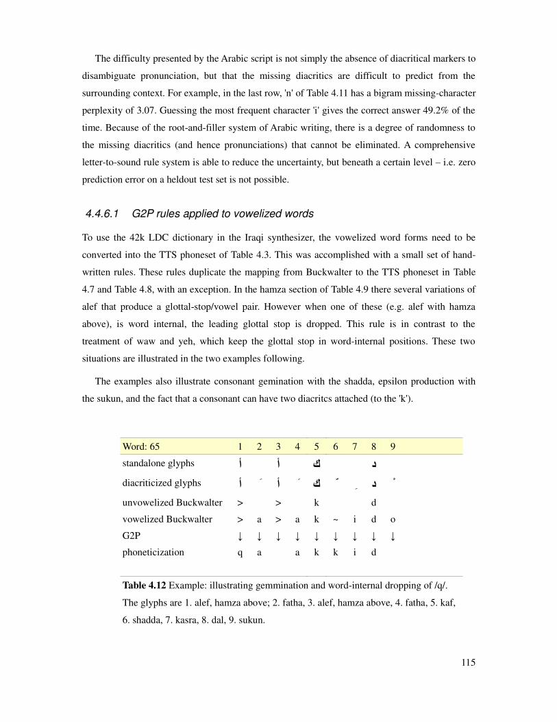
The difficulty presented by the Arabic script is not simply the absence of diacritical markers to

disambiguate pronunciation, but that the missing diacritics are difficult to predict from the

surrounding context. For example, in the last row, 'n' of Table 4.11 has a bigram missing-character

perplexity of 3.07. Guessing the most frequent character 'i' gives the correct answer 49.2% of the

time. Because of the root-and-filler system of Arabic writing, there is a degree of randomness to

the missing diacritics (and hence pronunciations) that cannot be eliminated. A comprehensive

letter-to-sound rule system is able to reduce the uncertainty, but beneath a certain level – i.e. zero

prediction error on a heldout test set is not possible.

4.4.6.1 G2P rules applied to vowelized words

To use the 42k LDC dictionary in the Iraqi synthesizer, the vowelized word forms need to be

converted into the TTS phoneset of Table 4.3. This was accomplished with a small set of hand-

written rules. These rules duplicate the mapping from Buckwalter to the TTS phoneset in Table

4.7 and Table 4.8, with an exception. In the hamza section of Table 4.9 there several variations of

alef that produce a glottal-stop/vowel pair. However when one of these (e.g. alef with hamza

above), is word internal, the leading glottal stop is dropped. This rule is in contrast to the

treatment of waw and yeh, which keep the glottal stop in word-internal positions. These two

situations are illustrated in the two examples following.

The examples also illustrate consonant gemination with the shadda, epsilon production with

the sukun, and the fact that a consonant can have two diacritcs attached (to the 'k').

Word: 65 1 2 3 4 5 6 7 8 9

standalone glyphs أ أ ك دdiacriticized glyphs أ أ ك د unvowelized Buckwalter > > k d

vowelized Buckwalter > a > a k ~ i d o

G2P ↓ ↓ ↓ ↓ ↓ ↓ ↓ ↓ ↓

phoneticization q a a k k i d

Table 4.12 Example: illustrating gemmination and word-internal dropping of /q/.

The glyphs are 1. alef, hamza above; 2. fatha, 3. alef, hamza above, 4. fatha, 5. kaf,

6. shadda, 7. kasra, 8. dal, 9. sukun.

115

Word: 66 1 2 3 4 5 6 7 8

standalone glyphs أ ؤ ج رdiacriticized glyphs أ ؤ ج ر unvowelized Buckwalter > & j r

vowelized Buckwalter > u & a j ~ r o

G2P ↓ ↓ ↓ ↓ ↓ ↓ ↓ ↓

phoneticization q u q u a jh jh r

Table 4.13 Example: illustrating gemmination and word-internal production to a

/q u/ pair. The glyphs are 1. alef, hamza above; 2. damma, 3. waw, hamza above, 4.

fatha, 5. jeem, 6. shadda, 7. reh, 8. sukun.

4.4.6.2 P2P rules from Arabic to English

In preparation for review of the English version of the Iraqi lexicon, it is necessary to convert

phonesets across languages so that the LDC 42k dictionary and Named Entity dictionary can be

spoken by the English synthesizer. The first issue is deciding what to do with phonemes not

present in the target language. These rules are summarized in Table 4.14 below.

Iraqi phoneme rule1 rule2

dq d

gq g

kq k

qq k

sq s

tq t

x k h

xq epsilon

q epsilon

hq h / _ V, [k,kq,qq] _ epsilon / _

h h / _ V, [k,kq,qq] _ epsilon / _

l l l l l

C C C ax C

Table 4.14 Rules to transfrom from Iraqi to English

phoneset. C is a consonant, V a vowel, and 'l l l' a triple /l/.

116

4.4.6.3 Cross-word interaction affecting pronunciation

One other major factor affects the relationship between written and spoken Arabic, and needs to

be mentioned, even though it is not addressed in this work. This is the fact that in Arabic, every

word is written (vowelized or not) as if it were spoken in isolation. However, according to the

rules of Arabic grammar, agreement of casing between subject and object result in the

corresponding words to alter their pronunciation. This long-range alteration occurs even though

there is no change to the written form. There are implications for both ASR and TTS. Preventing

the synthesizer from mispronouncing words therefore requires a part-of-speech tagger and a

lexicon annotated with parts of speech variants. Our current work does not attempt to make such

advanced distinctions.

4.5 Lexicon verification using native speakers

The task of verifying and correcting pronunciations for the named entity list serves two purposes.

First is to have the English synthesizer pronounce the Arabic words as accurately as possible,

given the constraint that many of the Iraqi phonemes can only be approximated. Second is to

enhance the Iraqi ASR lexicon with more accurate pronunciations so that the word error rate on

named entities decreases. The basic idea is to have the native speakers listen to synthesized

versions of each word (pronounced in isolation), and to select the best variant. This is obviously

appropriate for the first purpose. For the purpose of ASR it is not evident that better sounding

pronunciations will transfer directly to better recognition, but is a reasonable working hypothesis.

This section concentrates on measurements of human performance, including the average amount

of time spent examining each word.

4.5.1 Application user interface

A pair of screen snapshots on the page 120 exhibits the lexicon verification interface. The current

word is displayed at the top in Arabic script along with an English translation. Beneath are up to

six alternate pronunciations for the word. We chose to display a phoneticized version of the

pronunciation for each alternative, rather than presenting each option blind. The user clicks the

neighboring Play button to hear the synthesized version. If none of the suggestions are adequate

the user selects “none of the above” and may optionally add a comment in the type-in box at the

bottom. In this situation the policy is as follows: if the best predicted pronunciation is not quite

117

correct but does not alter the word's meaning, the reviewer is encouraged to select that version. If

the mispronunciation alters the word meaning, then “none of the above” is required. When a new

word is presented the default is “none of the above” in order to encourage the user to make an

active selection.

The interface is designed to be as simple as possible. Each of our two native speakers was

provided a training session. In the training session the user was given brief instructions on how to

operate the program, and then handed over to try themselves. During the subsequent hour the user

would work through the first 50 words or so, and be invited to ask questions at any point. The

interactive training session is useful for catching systematic problems. For example, in preparing

the English pronunciations the Arabic phoneset was hand-mapped onto the English phoneset.

Originally the mapping contained the entries /¿/ _ /k/ and /q/ _ /nil/. It was discovered

during the familiarization session, in what came to be called “the k problem,” that these mapping

needed to be swapped. This correction is reflected in Table 4.14.

Feedback during the training day helped refine the program. This included the location of the

buttons, the size of the fonts (bigger), and the loudness of the wavefiles (louder). So that they

may work remotely, each user was provided a laptop with the verification software loaded and

configured. After every few days the user came into the lab to offload data and to discuss issues,

such as whether the built-in speaker is adequate or if headsets are preferred. A couple practical

experiences are worth sharing. One is to remind users that there exist “little speaker buttons” on

the laptop keyboard, that mute should be turned off, and the speaker volume set high. Another is

to ensure that the user's selection from previous sessions can be reviewed, lest they think that

their efforts have been lost. For sake of simplicity, the program of Figure 4.4 (see page 120) had

no File|Save or File|Load options – it would automatically start up at the first un-reviewed word.

A design oversight was in not automatically loading all past stored results, even though this slows

program initialization. Before beginning to work on a new batch of words in earnest, users like to

go backwards and remind themselves of where the left off. This deficiency was corrected before

the majority of work commenced.

An obvious weakness of the program is that if the correct pronunciation is not listed, the user

can only provide corrective information by writing a comment. Though neither reviewer is

trained in linguistics, both grasped the idea of sounded-out spellings and asked for a chart

showing how the Arabic characters were converted into this representation. They also liked the

idea of typing their own phoneticization and having it synthesized. This more advanced feature

was added later in version 2, and can be seen in the bottom image of Figure 4.4.

118

After several sessions, it became apparent the reviews had a serious complaint. Because the

Arabic words were presented without diacritic markings, many of the words were ambiguous.

One possible vowelization for “badir” might mean “moon”, while for another “in lieu of”. One

reviewer estimated the occurrence of ambiguous words at 10%. This problem was reduced

somewhat by the fact that words are nouns (making moon the right guess). One reviewer added

that because the system targeted the southern dialect of Iraqi Arabic, he could use that knowledge

to help infer which word was intended. Still, the strong preference was expressed that the word

should be accompanied by the intended meaning, or clarified by the surrounding context in which

it occurs. Since the named entity word lists came without such information, this request could not

easily be met.

As another approach to refining pronunciations, one reviewer suggested that the program

allow him to annotate the Arabic word by adding the missing diacritics. This idea, while

attractive, also presented a challenge: even specialized Arabic keyboards have no keys assigned to

the diacritic characters7. This direct-editing approach has pros and cons. The advantage is that the

reviewers are working with the written script, which is more familiar than using an phonetic

alphabet. However, adding diacritics is not a normal procedure when writing Arabic – speakers

have little practice at this, and tend to transcribe what they think the markup should be, rather

than on actual pronunciation. Also, this approach would not be appropriate should the native

speakers not be literate. We had the good fortune of working with two users holding advanced

degrees.

7 After a certain amount of exposure, though, one of the users became wise to the synthesizer and

requested the “internal code” that converts graphemes to sounds.

119

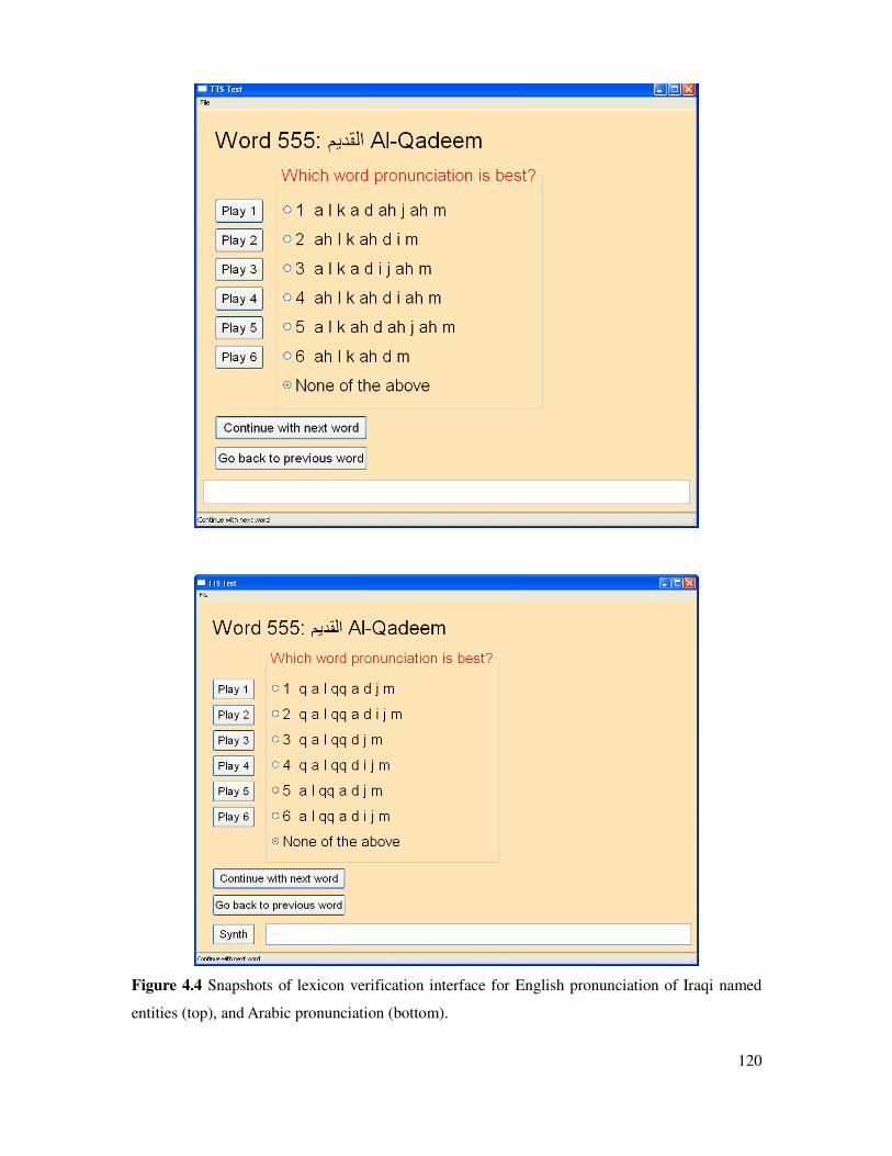
Figure 4.4 Snapshots of lexicon verification interface for English pronunciation of Iraqi named

entities (top), and Arabic pronunciation (bottom).

120

4.5.2 Measurement protocol

A person managing an effort such as the TransTac project want to know much it costs to have the

lexicon corrected by human review, and whether it is worth the cost. Ultimately, one wants to

know how many dollars it costs to reduce the ASR word error rate by 1%, or to reduce the TTS

mispronunciation rate by 1%. For the moment we may address the easier to answer question of

“how may words can be reviewed in one hour?”.

To help answer this question the lexicon review program wrote detailed log files of user

actions. The actions include when and how many times a wavefile was played, the selections

made, and the time spent moving between words. Figure 4.5 illustrates a typical timeline with the

relevant actions indicated. The user loads a new word by clicking “continue with next word” or

“go back to previous word”. There is a span of time in which the user plays and listens to the

wavefiles. He clicks one of the of radio buttons to make a selection. The selection often occurs

after all the wavefiles are played. But it is not unusual for the reviewer to play several, make a

selection, and then play several more to double-check. Finally, the decision is confirmed by

moving on to the next word.

Figure 4.5 Timeline of user actions. Indicated points are: loading a new word, playing wavefiles,

selecting a choice, and deciding to move on to the next word.

Given this usage pattern, we measure the average time of the following actions.

1. Preparing. The time from when a new word is loaded to when the first wavefile is played.

2. Playing. The time from initiating the play of the first wavefile, to the end of the last.

3. Deciding. The time from when the last wavefile finished playing to when decision is

confirmed by moving onto the next word.

121

playingpreparing

deciding

total time on word 2total time on word 1

4. Short breaks. These are pauses in the logfile that suggest the user has taken a short break,

such as to fetch a cup of coffee or to dispose of its processed form. As in a normal office

environment, short breaks are considered a part of being on the job.

5. Long breaks. These are pauses in the logfile that suggest the user has moved onto some

other activity, such as having dinner.

Breaks could not be explicitly measured since the lexicon review program offered no mechanism

for logging on and logging off. Even if it did, one can't rely on the user being diligent in that

regard. So some means of detecting breaks is needed in any event. The threshold of a short break

was set to two minutes, and a long break to 30 minutes. There is a degree of arbitrariness to these

thresholds and changing them adjusts the following numerical results slightly. A long break was

defined as 30 minutes since, in order to get paid, the reviewers maintained a time sheet with half

hour resolution. (Participants were assured that the log files would not be used to compute their

weekly pay.) When computing average times of preparing, playing, and deciding, the breaks are

filtered out. Long breaks are discarded entirely.

4.5.3 Human efficiency measurements

The lexicon review application writes a logfile of all user actions including the playing of

wavefiles, making selections, typing in comments, and navigating the word list. In mining

information from the logfiles a picture emerges of where the human effort goes. Multi-choice

word selection experiments do not exist in the literature, making this information novel.

It is worth repeating that reviewer A worked exclusively on the Iraqi named entity

pronunciations, while reviewer B worked exclusively on the English pronunciations. The

ordering of words in each list were exactly parallel; however, the suggested pronunciations for a

given word do not correspond across tasks. Also, the synthesizers used to generate pronunciation

wavefiles were built from different speakers, from unequal amounts of speech. Despite the non-

identical working conditions, we will boldly place the two users under comparison. User A was

able to devote more time to this task than B, and so completed a larger portion of the word list.

Users A and B show similar words-per-minute performance levels, as well as some interesting

differences in usage patterns (see section 4.5.4 ). On average, each reviewer spent the same

amount of time per word – about 37-39 seconds, or 30-32 seconds discounting short breaks. Two

words per minute is what a person using this application can accomplish undistracted. When

including all forms of overhead, a manager should plan according to one word per minute.

122

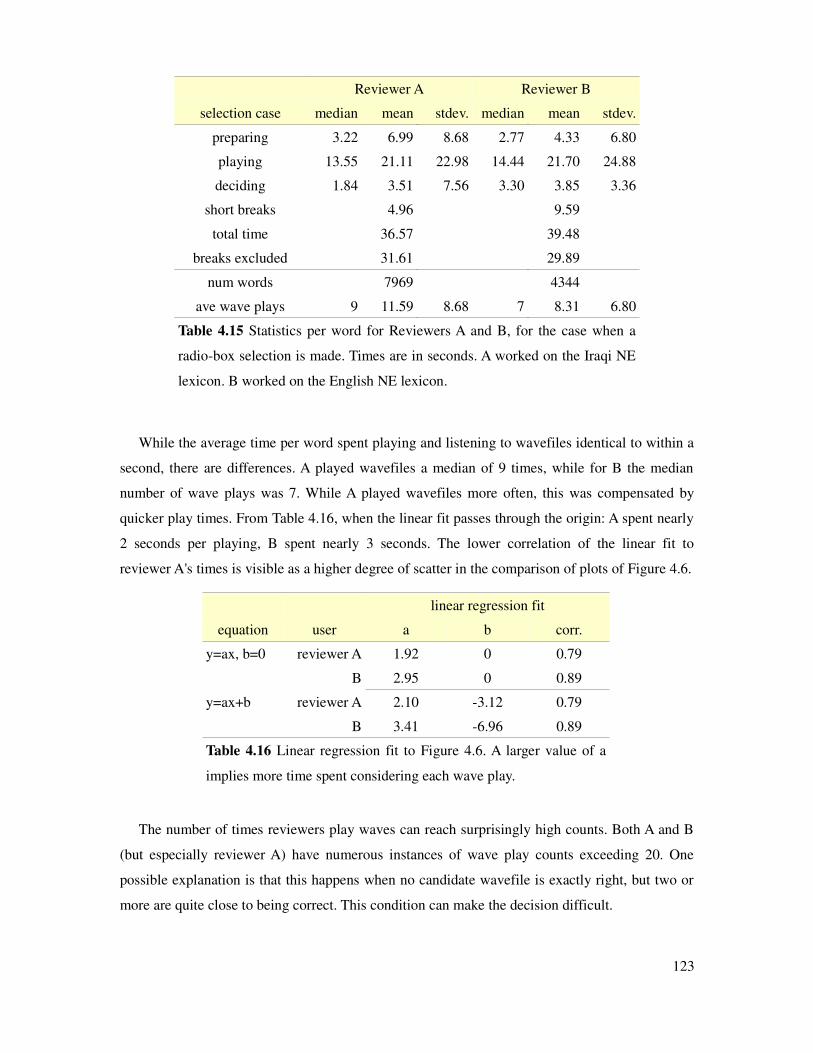
Reviewer A Reviewer B

selection case median mean stdev. median mean stdev.

preparing 3.22 6.99 8.68 2.77 4.33 6.80

playing 13.55 21.11 22.98 14.44 21.70 24.88

deciding 1.84 3.51 7.56 3.30 3.85 3.36

short breaks 4.96 9.59

total time 36.57 39.48

breaks excluded 31.61 29.89

num words 7969 4344

ave wave plays 9 11.59 8.68 7 8.31 6.80

Table 4.15 Statistics per word for Reviewers A and B, for the case when a

radio-box selection is made. Times are in seconds. A worked on the Iraqi NE

lexicon. B worked on the English NE lexicon.

While the average time per word spent playing and listening to wavefiles identical to within a

second, there are differences. A played wavefiles a median of 9 times, while for B the median

number of wave plays was 7. While A played wavefiles more often, this was compensated by

quicker play times. From Table 4.16, when the linear fit passes through the origin: A spent nearly

2 seconds per playing, B spent nearly 3 seconds. The lower correlation of the linear fit to

reviewer A's times is visible as a higher degree of scatter in the comparison of plots of Figure 4.6.

linear regression fit

equation user a b corr.

y=ax, b=0 reviewer A 1.92 0 0.79

B 2.95 0 0.89

y=ax+b reviewer A 2.10 -3.12 0.79

B 3.41 -6.96 0.89

Table 4.16 Linear regression fit to Figure 4.6. A larger value of a

implies more time spent considering each wave play.

The number of times reviewers play waves can reach surprisingly high counts. Both A and B

(but especially reviewer A) have numerous instances of wave play counts exceeding 20. One

possible explanation is that this happens when no candidate wavefile is exactly right, but two or

more are quite close to being correct. This condition can make the decision difficult.

123

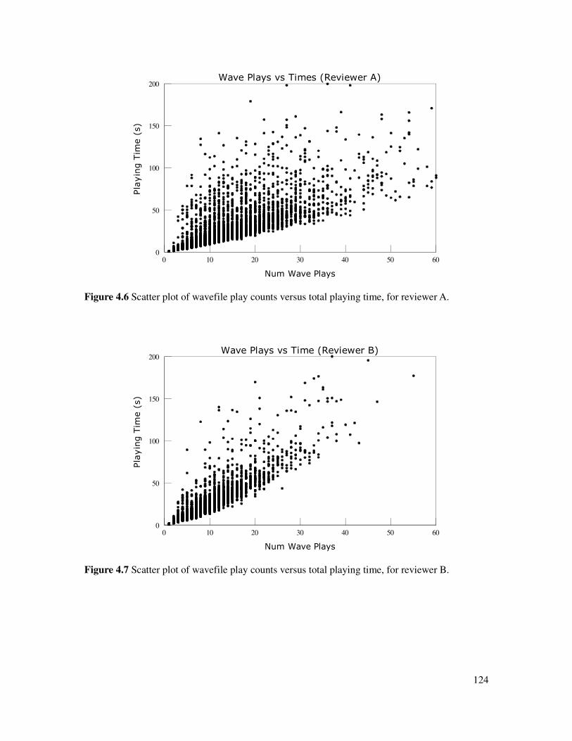
124

Figure 4.6 Scatter plot of wavefile play counts versus total playing time, for reviewer A.

Figure 4.7 Scatter plot of wavefile play counts versus total playing time, for reviewer B.

Num Wave Plays

0 10 20 30 40 50 60

Playing Tim

e (s)

0

50

100

150

200Wave Plays vs Times (Reviewer A)

Num Wave Plays

0 10 20 30 40 50 60

Playing Tim

e (s)

0

50

100

150

200Wave Plays vs Time (Reviewer B)

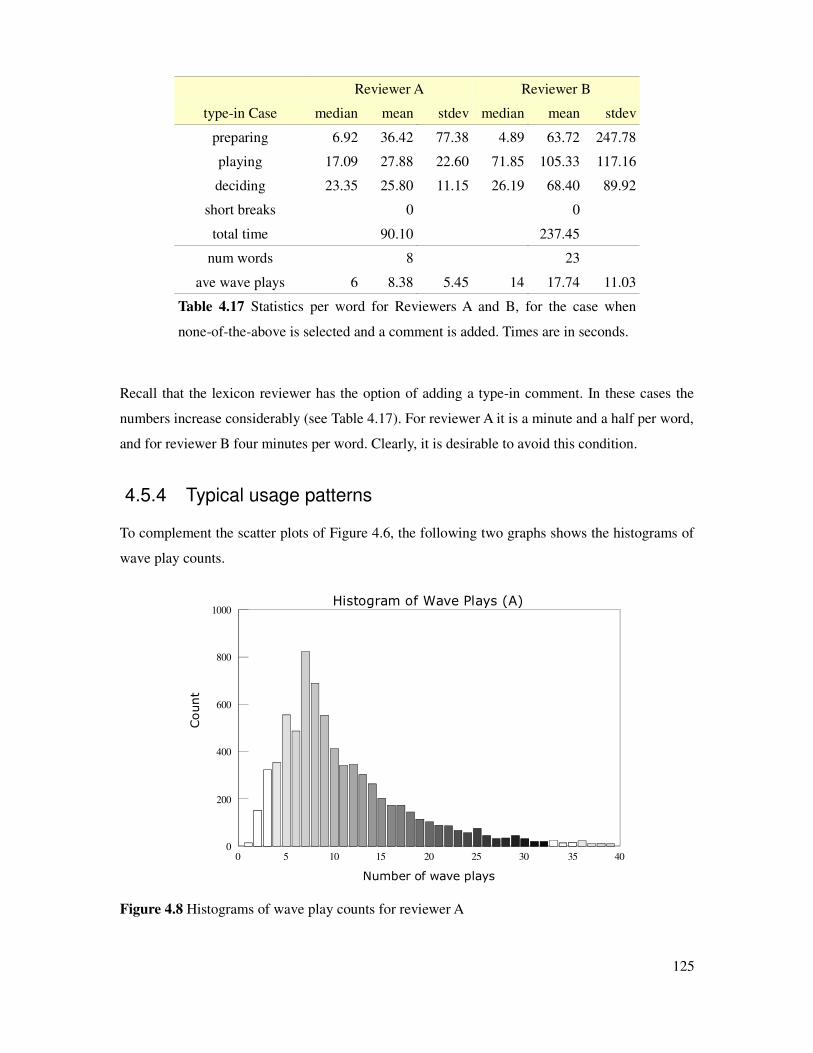
Reviewer A Reviewer B

type-in Case median mean stdev median mean stdev

preparing 6.92 36.42 77.38 4.89 63.72 247.78

playing 17.09 27.88 22.60 71.85 105.33 117.16

deciding 23.35 25.80 11.15 26.19 68.40 89.92

short breaks 0 0

total time 90.10 237.45

num words 8 23

ave wave plays 6 8.38 5.45 14 17.74 11.03

Table 4.17 Statistics per word for Reviewers A and B, for the case when

none-of-the-above is selected and a comment is added. Times are in seconds.

Recall that the lexicon reviewer has the option of adding a type-in comment. In these cases the

numbers increase considerably (see Table 4.17). For reviewer A it is a minute and a half per word,

and for reviewer B four minutes per word. Clearly, it is desirable to avoid this condition.

4.5.4 Typical usage patterns

To complement the scatter plots of Figure 4.6, the following two graphs shows the histograms of

wave play counts.

Figure 4.8 Histograms of wave play counts for reviewer A

125

Number of wave plays

0 5 10 15 20 25 30 35 40

Count

0

200

400

600

800

1000Histogram of Wave Plays (A)

Figure 4.9 Histograms of wave play counts for reviewer B. Added for comparison is the curve of

a Poisson process with lambda = 7.5. The Poisson process defines a pdf of P k ; = e−

k ! and

corresponds to a random variable which has an average event frequency per unit of time.

Of these two histograms, Figure 4.9 in particular exhibits a curious bimodal distribution. There is

a strong peak at n=2 and a second strong peak at n=7. Based on in-person observation and review

of the log files, this is likely due to there being two distinct modes of evaluation. Call these Mode

I and Mode II. In Mode I the dominant action is as follows: the reviewers plays the first wavefile,

likes it, checks the second, then selects the first. This accounts for the peak at n=2. In Mode II, the

reviewer plays all six wavefiles, plays the one he likes most a second time (for confirmation),

then selects it. This accounts for the peak at n=7. There will be random variation about each peak

– the user may play the favored wavefile three times, for example, or only once.8 Playing each

presented wavefile at least once can be the defining line between modes. Informally, Mode II is

“comprehensive checking” while Mode I is akin to “you know it when you hear it.”

This notion of “modes of evaluation” can be investigated by examining the most common

patterns of play. Let each wavefile have a number 1..n, with 0 assigned to “none of the above”. In

the notation of the following list, a pattern of 121 means that 3 wavefiles were played: the first

followed by the second followed by the first again (then a decision was made). Similarly,

1234561 means that all six were played in sequence, followed by the first once more.

8 In a fraction of cases there are fewer than six candidates available, which acts to blur the distribution.

126

Number of Wave Plays

0 5 10 15 20 25 30 35 40

Count

0

200

400

600

Histogram of Wave Plays (Reviewer B)

Reviewer A Reviewer B

rank count pattern mode count pattern mode

1 199 121 I 636 12 I

2 134 1234561 II 208 1 I

3 122 11 I 198 123 I

4 121 12341 I 151 1234561 II

5 103 1211 I 127 1234 I

6 92 1234565 II 104 123456 II

7 76 1234564 II 53 12345 I

8 76 111 I 44 1234564 II

9 73 12343 I 40 1231 I

10 66 1234562 II 40 112 I

11 66 12121 I 39 1234565 II

12 66 1212 I 37 1234563 II

13 61 1234563 II 35 122 I

14 55 122 I 29 1234562 II

15 51 12342 I 28 123451 I or II

429 123456x II 413 123456x II

Table 4.18 Most common patterns of wavefile play sequences. The pattern

123456x combines those instances in which all six wavefiles are played in

sequence, optionally followed by a repeat of one of the six.

In examining the patterns for reviewer B we attribute to mode I short patterns such as 12, 1, 123,

1234, 1231, 112. Not all wavefiles are played every time. The mode II patterns include

123456x, 123456, 123451, 12345621. It is possible that displaying the phonetic string beside

each wavefile accounts for the mode I pattern. Reviewer A also has some mode I patterns in

which repetition among a pair of wavefiles figures prominently, as seen in the set 1211, 111,

1212, 12121, 122. Naturally, in cases where the number of plays is large, it is fair to conclude

that the word is difficult to decide.

For reviewer B, the first three wavefiles are played more than once, on average, while the last

three are played less than once. This tendency was taken into consideration when the program

was designed; the predictions are intentionally ranked according to estimated probability of being

correct. Play frequency is plotted in Figure 4.10.

127

Reviewer A Reviewer B

select play ratio selection percent play ratio selection percent

0 – 121 4.86 – 107 2.43

1 3.060 895 35.94 1.917 1397 31.66

2 2.686 710 28.51 1.678 1302 29.51

3 2.559 385 15.46 1.283 578 13.10

4 2.346 203 8.15 1.212 501 11.36

5 2.283 123 4.94 1.024 305 6.91

6 1.778 53 2.13 0.933 222 5.03

Table 4.19 Play ratio is the average number of times wavefile n is played. The

selection percentage indicates how often wavefile n was selected.

Figure 4.10 Histogram of wave files played, by wave number, normalized to 1.0

4.5.5 Comparison to the literature

We find that user A and user B spend the same amount of time per word, on average 35s, even

though their patterns of usage show distinct differences. An average of 35s per Iraqi word is

substantially higher than the time of 10.3s reported in the literature by Davel and Barnard for

Afrikaans [48] In a later publication the authors report an average of 3.9s per word when

extending the Afrikaans dictionary from a size of 7782 to 20,204 words [56]. In analyzing the

128

Wavefile Number

1 2 3 4 5 6

Play Frequency

0.2

0.6

1.0

1.4

Normalized Wave Play Histogram

distribution of reviewer times – using a histogram bin size of 1 second – the authors find the most

frequent review time to be 1 second (3700 of 12,422), with the second most frequent time 2

seconds (3500 cases). The DictionaryMaker software they used for lexicon review plays a

wavefile of the predicted pronunciation when the user moves to the next word [63]. The wavefile

is a concatenated sequence of phonemes recorded in isolation. In our examination of the software,

using the bundled Afrikaans project, we noted detectable gaps between each phone in the

synthesized wavefile, and that the combined time most often is 2-4 seconds. This implies that the

user review times reported in [56] excludes wave play times. Also, the authors consider a break to

be 30s, while we use a threshold of 2 minutes.

In our Iraqi lexicon building experience, the preparation and decision times introduce a fairly

fixed overhead of 8.2 to 10.5 seconds (Table 4.15). Total playing time is the largest variable

factor, and depends on the number of times the candidate wavefiles are played and considered.

The average time per play was 2.1 and 3.4s for reviewer A and B respectively (Table 4.16).

Average time per word can be reduced by restricting the number of plays permitted. However,

quality of the results will suffer. Permitting unlimited time per word supports the reviewer in

being maximally confident about their choice.

4.5.6 Improvement in ASR word error rate

In an experiment to evaluate the impact Iraqi decoder performance, several improvements were

tested on the May 2008 Names task. This is a designated test set in which one named entity

appears in each utterance. 4.20 summarized the effect of the new lexicon and of a new language

model, as compared to the 2007 system. The new (class-based trigram) language model provided

a 7.7% relative improvement. The new lexicon provided an addition 1.9% relative improvement

(0.7% absolute).

Iraqi

lexicon

language

model

word

error rate

relative

improvement

old old 40.2

old new 37.1 7.7

new new 36.4 1.9

4.20 Effect of new Named Entity lexicon on WER for the

Transtac May 2008 Names task. Values are percentages.

129

4.6 Summary

In this chapter we deployed lexicon building tools out “in the field” for the very difficult language

of Arabic. Two bilingual native speakers were employed in this task. Each reviewed words from

the Transtac Named Entity list. One worked with the Iraqi Arabic synthesizer, completing nearly

8000 words. The second worked with the English synthesizer, completing nearly 4400 words.

Breaks excluded, the task completion time averaged 30-32 seconds per word. The number of

wavefile plays per word varied considerably. For some words the reviewers listened to the

suggested wavefiles over 50 times. Other, presumably easier, words required only one or two

listens. With six wavefiles presented per word, the median number of plays was seven. The most

common usage patterns show that reviewers listen to each wavefile once, perform a double-check

on one, then make a selection. Typing in a correction is to be avoided. When the reviewers found

this necessary the average task times increased from to 1.5 minutes (reviewer A) and 4 minutes

(reviewer B).

The next chapter investigates lexicon building in the context of building synthesizers from the

ground up, using very little data.

130

5 Voices From Little Data

This chapter has three purposes. The first is to collect data on the process of building synthetic

voices from little data, for English and non-English languages (Kominek et al. 2006, Schultz et

al. 2007) [104][140]. The second is to provide a framework for evaluating the quality of synthetic

voices in relation to the effort put into the voice development process (Kominek et al. 2007)

[105]. The third is to demonstrate methods for iteratively improving a synthesizer that has been

built from little data (Kominek et al. 2008) [106]. In pursuit of these goals we introduce a novel

way of establishing the relationship between objective and subjective quality measures. This

information allows a voice-building system to evaluate and guide the user's progress.

We want to know when a voice is good, when a measured improvement is significant, and

what level of quality can be expected for a given amount of effort. Effort is measured as the

amount of time taken to complete a task. Quality may be a measured using an objective,

subjective, or semi-subjective measure. Objective measures do not involve a listener. Subjective

tests ask a listener to make preference decisions. In what may be termed semi-subjective, such

tests ask a listener to perform an objective task – most commonly word transcription. Each

category has several possibilities, including the following.

objective

1. mean mel cepstral distortion (MCD) measure the spectral distance between an

original and resynthesized waveform.

2. pitch distortion measures the difference between the original and predicted F0

curve.

3. duration model error measures the root mean square error between predicted and

actual phoneme lengths.

131

subjective

1. 5-point MOS scale asks users to rate a voice on a scale of 1 to 5, where 1 is taken

to mean “poor” and 5 “excellent”. The scores are usually assigned on a sentence-by-

sentence basis, and are typically averaged to yield an overall score.

2. AB tests asks users to compare two versions of the same utterance and to choose

the one that they prefer.

3. AB-tie tests are similar to AB except that the user has the option of declaring the

competition between wavefiles a tie.

4. ABX tests again provide two candidates (A and B) plus a reference wavefile X. The

user is asked which of A and B is most similar to X.

semi-subjective

1. In-domain sentence transcription asks a user to transcribe the words in an

utterance. The utterance may be played once or multiple times, depending on the

experimental protocol. The test is said to be in-domain if the test and training

sentences are drawn from prompt lists having similar vocabulary, syntax, etc.

2. Out-of-domain sentence transcription is similar, except that the test sentences are

“different” in some proscribed way from the training data.

3. Isolated word transcription presents single isolated words, and similarly may be

in-domain or out-of-vocabulary words.

4. Carrier sentence transcription places a target word within a fixed sentence, and

asks the user to identify the word; e.g. “Now we will say X again”. Popular are the

Diagnostic Rhyme Test (DRT) and the Modified Diagnostic Rhyme Test (MRT)

5. In Semantically Unpredictable Sentence (SUS) transcription the user is presented

with “nonsense” sentences that minimizes the user's expectations due to language

familiarity. This is the most challenging test and can only be successfully performed

by native speakers.

6. Memory load tests ask the user to listen to a largish chunk of information about,

e.g. bus stop information, and to answer questions afterwards.

7. Task-oriented tests ask the user to obey instructions or perform some functional

activity, such as “open the release valve on the cooling pipe.”

132

In this work we adopt three primary testing tools, that of mean mel cepstral distortion (MCD),

AB-tie preference tests, and in-domain sentence transcription. This provides three angles on voice

quality, and yields data for correlating objective, subjective, and semi-subjective measurements.

While measuring voice quality through various means is well and good, we want to apply

what we know to new languages. That is, when a user is working on their own (minority)

language, it would be of great value to be able to say, in effect, “based on experience with other

languages, your synthesizer has a quality rating of fair.” Even more valuable would be to then

recommend a course of action, such as: “to make your synthesizer good, record these 500 extra

utterances and provide pronunciations for this list of 900 words.” We contend that the ability to

make such an assessment requires a calibrated frame of reference.

To provide a calibrated frame of reference, in this chapter we present a large set of empirical

experiments conducted on English to measure how a voice improves with time and effort. The

basic premise is that a pair of complementary English voices – one “good” and one “bad” – can

serve as landmark points for voices built in non-English languages. We take the term good to

mean a voice with a large amount of speech and an accurate pronunciation dictionary, and bad to

mean a small voice with a minimal or poor dictionary. To compensate for the effect of database

size, pairs of good/bad calibration-voices are built from identical amounts of speech, ranging

from a couple minutes to several hours. The resulting frame of reference is a set of connected

points of (MCD, database size) pairs. This is taken up in detail next, in section 5.1 .

Section Error: Reference source not found provides results on AB-tie preference tests, in

which the user chooses from voices build from different amounts of speech, and/or a lexicon of

different coverage. Section 5.3.1 provides results of transcription tests. Again, two dimensions

are varied: the amount of speech used to build the voice, and the quality of the lexicon. Section

Error: Reference source not found investigates the correlation between the objective and

subjective measurements. Our experiments offer insights into this little-understood relation. We

observe, for example, where MCD breaks down as an objective measure of voice quality.

The issue of effort allocation is taken up in Section Error: Reference source not found. The

question we seek to answer is: is it more effective to concentrate on the lexicon, or to simply

record more speech? Or if both are important, is there a preferred ordering of tasks? Naturally the

answer is both language-dependent and user-dependent. The complexity of a languages G2P rules

matters, as does the speed at which the user can perform the voice building tasks of recording and

pronunciation definition. Nonetheless, experiments with English suggests that lexical work

contributes substantially only once a sufficient base of speech (of about 15 minutes) has been

133

collected and distilled.

Finally, section 5.2.2 examines eight small-scale Non-English voices built from limited data.

The experimental results of Section 5.2 allow us to evaluate the MCD values for the following:

French, German, Bulgarian, Hindi, Tamil, Konkani, Mandarin, and Vietnamese. In addition,

preliminary transcription tests were performed for German, Bulgarian and Hindi.

5.1 Effect of CART tree training conditions on MCD

Because the training of CART trees is a crucial component in the creation of Festival voices used

in this work, it is important to understand how they respond under different training conditions.

The training conditions include these four variables: the particular set of prediction features, the

amount of speech in the training set, the labeling of the speech, and the stop value employed

during training. To develop a thorough, empirical understanding, we pose the following

questions.

How important are the language-dependent features in CART tree training?

What are the most important features in the CART tree training?

What context size window (neighborhood) is sufficient for context-dependent features?

What stop value – as it affects the minimal leaf node size – is optimal?

How does MCD respond to the conditions of under-fitting (large stop value) and over-

fitting (small stop value)?

At what rate does a voice improve as more speech is collected?

Is there a threshold beyond which collecting additional speech offers little added benefit?

To what extent is the distortion curve speaker-dependent?

The question of language dependency is placed first in this list for its application-specific

relevance. If building quality voices is highly dependent on language-dependent features (as will

be defined shortly) then this places greater demand on users – because they will be expected to

provide this information. Conversely, if such features are not highly important, then the burden on

users is lessened, and the ability to apply these tools in a multilingual setting is enhanced.

134

5.1.1 Experimental data and testing protocol

To answer the questions posed in the previous section we undertook systematic experiments

involving two databases. This section briefly describes the data and experimental protocol.

5.1.1.1 Database selection

Two English databases are used for the purpose of calibration. The first is arctic_slt from the

Arctic database suite [100][101]. This consists of nearly one hour of carefully read speech,

recorded in a single day under low noise conditions (in a sound isolated room) with quality audio

equipment set at a sampling rate of 32 kHz. The utterances are sentences extracted from novels

available from the Gutenberg Project [78]. A representative sentence is “They will search for us

between their camp and Churchill.” The speaker possesses a West GA (general American) dialect

[114].

The second is a multi-hour database recorded by this author over multiple days in a quiet room

using a laptop, with a sampling rate of 16 kHz. This corpus is intended to mimic optimistic

conditions of SPICE users. That is, the recordings are less carefully monitored, contain noticeable

additive white background noise from fans and electronics, but no transient noise such as

background music, surrounding talkers, barking dogs, etc. The utterances are sentences and

phrases selected from cooking recipe instructions. Two representative examples are “sprinkle the

cavity with salt and pepper” and “in a small bowl, mix flour, beer, and sauce.” The speaker

possesses an Inland North Canadian accent [114].

For contrast, the two English databases have speakers of opposite gender (though similar age),

and cover different domains. Both are read speech, as that is appropriate for our task.

5.1.1.2 Training / testing data split

For the following experiments the data has been split 90/10% into training and test sets, with 10-

fold cross validation applied. In order to mitigate systematic changes over time, the test

utterances are uniformly selected from the full database at every 10th position. Let n be the zero-

based index number of each utterance, and p the partition number from [0..9]. Then the test set Sp

= n s.t. n mod 10 = p. When p=9 the test set contains the 10th, 20th, 30th utterance from the

database, and so on. Each experimental condition thus has 10 data points, from which the mean

and standard deviation is calculated.

135

5.1.1.3 Resynthesis and measurement

We adopt mean mel cepstral distortion as our objective measure. It's worth mentioning here that

the speech being evaluated is not generated from the text, but is copy-synthesized. This means

that the output exactly mimics the phoneme sequence, duration pattern, and pitch contour of the

original – all that is predicted is the sequence of cepstral coefficient vectors (one per frame). This

protocol also ensures exact alignment between the original and generated waveform, maximizing

the prediction error.

5.1.1.4 Variation of experimental conditions

The training of synthesizers involves numerous control parameters that may be varied, plus

dependencies on the size and quality of the speech data. The interaction among all the factors is

complex and not thoroughly investigates. The following sections attempt to systematically vary

training conditions, to isolate one factor (or set of similar factors) at a time, and to evaluate their

impact. We begin with the prediction features employed in CART tree learning.

5.1.2 Feature importance in CART tree training

In speech synthesis, the range of predictive features can range from a few dozen to over a

hundred. Examining the effect of each one in isolation would be an enormous task. To make the

problem tractable, we divide features into four classes.

name symbolics – language-independent name features

frame-position related features

IPA symbolics – language-dependent name features

linguistic features

Name symbolics include the name of the current phoneme and that of the immediate

neighborhood, plus the names of HMM states within a phoneme, and their neighbors. The

number of neighbors referenced on either side of the current unit determines the window size,

which typically ranges from 2-4.

Positional features are defined at the frame level, where each frame is typically 5 ms is length.

Features include the location of a frame within a state, e.g. how far it is from the starting time,

plus derivative values such as percentages. Feature may be integers, floating point values, or even

symbolic values if the range falls within a finite set. A possible question includes “is this frame at

136

the boundary between phones?” (yes or no).

IPA symbolics are a subset of International Phonetic Association-defined features. These

include manner and place of articulation for consonants, as well as height, frontness, and

roundness for vowels. The set of IPA features depends on and are derived from the phoneme set

of a given language. Consequently these are considered language-dependent – their values

depends on knowing the phonemes of a given language.

Linguistic features correspond to the output of high-level functions, such as parts-of-speech

taggers, routines that analyze words into syllables and assign stress. The exact identity of all

features is provided in Appendix A.

This classification into four groups is not arbitrary, but relates to the difficulty of acquiring the

respective information. Name symbolics requires only that each basic speech unit has a unique

name. Names may equate with the classical concept of phonemes, or may be graphemes, or some

other symbol set. Position values also share the property of being language-independent, but are

different in that they refer to the finest time resolution of frames (and are usually real-valued

numbers). IPA symbolic features, in contrast, are language-dependent and assume that a) the

names are phonemes, and b) the phoneme set is appropriate. This issue is highly relevant because

the ultimate target users of SPICE are people without deep background in phonetics. Finally, the

demands presented by linguistic features is even higher: namely, a computational linguist that can

program functions in Lisp.

Table 5.1 summarizes the feature categories. In our experiments we used a context window of

4 items. This explains, for example, why name symbolics has 16=2x8 features. The current

phoneme exists in a context of 4 to the left and 4 to the right. Likewise for the sub-phonetic

states. Note that while IPA symbolics has the most features at 72, the features take on only a small

numbers of values. For example vowel height has 4 values (high, mid, low, undefined), and vowel

roundness has 3 values (rounded, unrounded, undefined). In contrast, phones will assume 40-50

values, depending on the language, and state names three times that. On this basis alone one may

suspect that the set of IPA symbolics offers less predictive ability than name symbolics. As the

following sections show, this turns out to be the case.

137

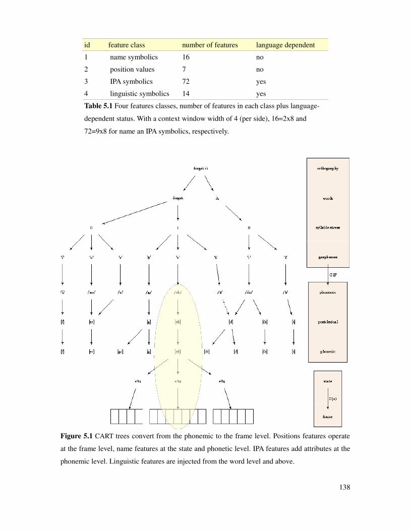
id feature class number of features language dependent

1 name symbolics 16 no

2 position values 7 no

3 IPA symbolics 72 yes

4 linguistic symbolics 14 yes

Table 5.1 Four features classes, number of features in each class plus language-

dependent status. With a context window width of 4 (per side), 16=2x8 and

72=9x8 for name an IPA symbolics, respectively.

Figure 5.1 CART trees convert from the phonemic to the frame level. Positions features operate

at the frame level, name features at the state and phonetic level. IPA features add attributes at the

phonemic level. Linguistic features are injected from the word level and above.

138

5.1.2.1 Feature importance by class / influence of stop value

If we give the shorthand names 1,2,3,4 to the four feature classes of Table 5.1, simple

combinatorics leads to 16 possibilities.

1 – default case of no CART trees

4 – features in isolation: 1, 2, 3, 4

6 – features in pairs: 12, 13, 14, 23, 24, 34

4 – features in triples: 123, 124, 134, 234

1 – all features combined: 1234

One less exhaustive strategy is a “stepwise” approach. First train the trees with the features

classes in isolation. The best performing class is identified and paired with the remaining 3. The

best pair is identified and the remaining features are added (two cases). Finally all features are

included.

Figure 5.2 plots the mean mel cepstral distortion curves for the four feature classes trained in

isolation, and the arctic_slt database. A set of voices were built with only name features, only

position features, only IPA symbolics, and only linguistic symbolics. Each curve has been

sampled at 20 stop values ranging from 2 to 8000. Recall that since lower MCD numbers are

better, the minimum point in these curves correspond to that curve's best voice.

As can be seen, linguistic information alone is the poorest predictor. It is also evident is that

the minimum points of the other three curves are all about equal. More precisely, they fall within

the standard deviation of the curves, which were measured to be in the range 0.04 to 0.06. Each

point plotted is the mean of a 10-fold cross-validation experiment. Despite the similar best values,

there are other differences. Notice that position features result in a broader basin. For small stop

values (below 50), IPA and name features shoot up more steeply – which indicates that they are

considerably more prone to over-fitting. Thus, position features provide the most robust

information.

139

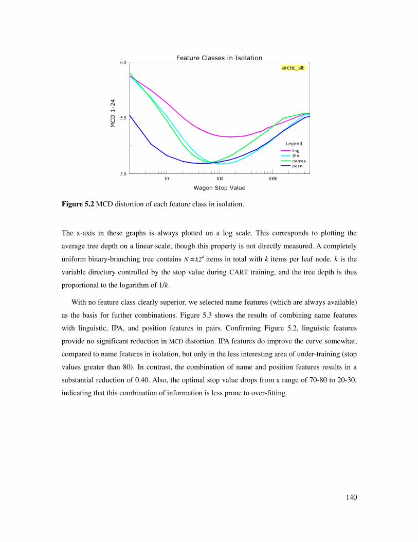
Figure 5.2 MCD distortion of each feature class in isolation.

The x-axis in these graphs is always plotted on a log scale. This corresponds to plotting the

average tree depth on a linear scale, though this property is not directly measured. A completely

uniform binary-branching tree contains N=k2d items in total with k items per leaf node. k is the

variable directory controlled by the stop value during CART training, and the tree depth is thus

proportional to the logarithm of 1/k.

With no feature class clearly superior, we selected name features (which are always available)

as the basis for further combinations. Figure 5.3 shows the results of combining name features

with linguistic, IPA, and position features in pairs. Confirming Figure 5.2, linguistic features

provide no significant reduction in MCD distortion. IPA features do improve the curve somewhat,

compared to name features in isolation, but only in the less interesting area of under-training (stop

values greater than 80). In contrast, the combination of name and position features results in a

substantial reduction of 0.40. Also, the optimal stop value drops from a range of 70-80 to 20-30,

indicating that this combination of information is less prone to over-fitting.

140

Legend

ling

IPA

names

posn

arctic_slt

Wagon Stop Value

10 100 1000

MCD 1-24

5.0

5.5

6.0Feature Classes in Isolation

Figure 5.3 MCD distortion of feature classes combined in pairs. The uppermost (names) curve is

included for reference.

To the “names + posn” pair, the addition of extra feature classes offers little improvement. Figure

5.4 shows the MCD curves for feature classes combined into triples, as well as all of them

together. The lack of predictive ability of the higher level “linguistic features” is in fact

encouraging. It implies that users do not need the expertise required to write the kind of high

level functions tested in these experiments.

Figure 5.4 MCD distortion of feature classes combined in triples, as well as the full set.

141

Wagon Stop Value

10 100 1000

MCD 1-24

4.6

4.8

5.0

5.2

5.4

5.63-4 Feature Classes

Legend

names + posn + ipa

names + posn + ling

names + posn + ipa + ling

arctic_slt

Wagon Stop Value

10 100 1000

MCD 1-24

4.5

5.0

5.5

6.0Feature Classes in Pairs

Legend

names

names + ling

names + IPA

names + posn

From these experiments we conclude that the language-neutral name and position features when

used in combination are sufficiently strong predictors for our needs. The IPA features contribute

only a modest amount, while linguistic features are not required. This is not to say that there is no

linguistic-class feature that may prove informative, or that there is no language in which IPA

features provide important information. It may be that in having tone variants explicitly marked

in tonal languages is essential, for example. But it does mean that even in the absence of

language-dependent training features, we remain on solid ground.

5.1.3 Effect of context width

In the experiments of the previous section the context width was set to 4. This applied both to

phone names and to phone-state names. With 3 HMM states per phone used during segmentation,

a context width of 4 equals one and one third phones. An argument can be made that in both cases

the context should reach equally to the left and right (4 phones = 12 states). But before drawing

that conclusion it is worth examining the actual effect of context width on prediction error.

In Figure 5.5 the CART trees have been trained using only state name features, with a context

ranging from 1 to 4 (the default). The results are not exactly what one might expect ahead of time.

Firstly, when increasing context width from 2 to 3 the reduction in MCD is slight. From 3 to 4 it

is non-existent. Secondly, large context width make the system more prone to over-fitting; when

the stop value is smaller than 25, the w=4 curve trends upward faster than the w=3 and w=2

curves. For larger stop values, the w=2, 3, and 4 curves overlap. The poor performance when w=1

is unsurprising. Consider that middle states (which are the most populous kind), the neighboring

features or a given phone will be the same, and therefore provides no predictive information.

While the pattern of Figure 5.5 contained some unexpected elements, Figure 5.6 came as a

complete surprise. The context width makes no difference at all for large stop value. For smaller

stop values (less than 60), w=1 is better than w=2, which is better than w=3, which in turn is

better than w=4. Evidently, adding extra phone context is lends to over-fitting.

When state context is combined with position feature, there is a strong additive effect, as

shown in Figure 5.7. As can be seen, the curves for w=2, 3, and 4 overlap almost exactly when

position features are included. Adding phone-based context (not shown) doesn't lower the curves.

The surprising conclusion is that phone context can be discarded from training, and that only a

width of 2 is really needed for state context. With out set of sufficient training features becoming

so lightweight, the natural follow-up question is: which of the position features are truly

necessary – is there redundancy that can be removed?

142

Figure 5.5 MCD distortion as a function of state name context width. These are the only features

used during training.

Figure 5.6 MCD distortion as a function of phone name context width. These are the only

features used during training.

143

Wagon Stop Value

10 100 1000

MCD 1-24

4.5

5.0

5.5

6.0Effect of Context Width - state names

width=4

width=1

Legend

state1

state2

state3

state4

Wagon Stop Value

10 100 1000

MCD 1-24

4.5

5.0

5.5

6.0Effect of Context Width - phone names

Legend

phone4

phone3

phone2

phone1

width=1

width=4

Figure 5.7 MCD distortion as a function of state name context width, combined with position

features.

5.1.4 Position features and a minimal training set

The Festival distribution for building CLUSTERGEN voices contains a feature description file

that defines seven position features, which has been adopted the experiments of this chapter. A

feature is “positional” if it describes the position of a (5 ms) frame within some speech unit.

There are three phone-related features, and four that are state-related.

The first, state_pos is a discrete feature with 3 values b,m,e. It asks if the current frame

the first (b), last (e), or in-between frame (m) within a state.

state_index counts the number of frames from the beginning.

state_rindex counts frames from the end.

state_place computes the ratio in from the beginning. For example, consider the 4th

frame of the 1st state of a phoneme.

state_pos=m,

state_index=3 (counting is zero-based),

state_rindex=7,

state_place=0.3.

144

Legend

state1

state2

state3

state4

state1 + posn

state2 + posn

state3 + posn

state4 + posn

Wagon Stop Value

10 100 1000

MCD 1-24

4.5

5.0

5.5

6.0Effect of Context Width - state names

width=4

width=1

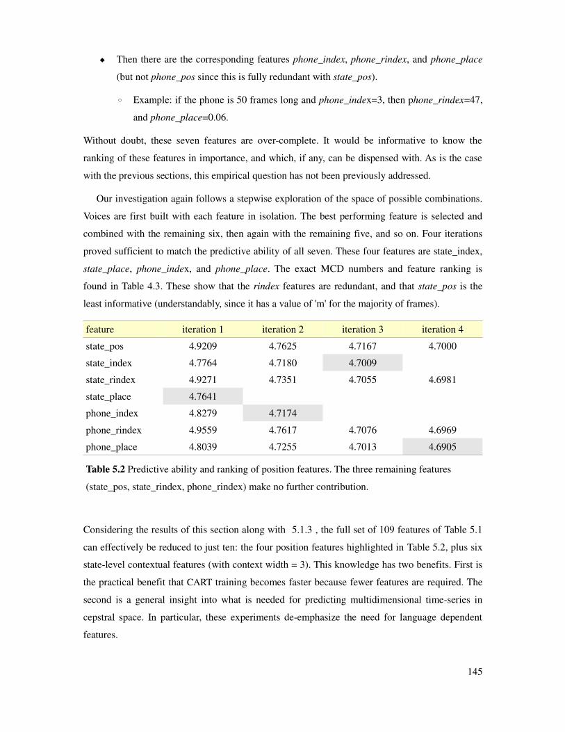
Then there are the corresponding features phone_index, phone_rindex, and phone_place

(but not phone_pos since this is fully redundant with state_pos).

Example: if the phone is 50 frames long and phone_index=3, then phone_rindex=47,

and phone_place=0.06.

Without doubt, these seven features are over-complete. It would be informative to know the

ranking of these features in importance, and which, if any, can be dispensed with. As is the case

with the previous sections, this empirical question has not been previously addressed.

Our investigation again follows a stepwise exploration of the space of possible combinations.

Voices are first built with each feature in isolation. The best performing feature is selected and

combined with the remaining six, then again with the remaining five, and so on. Four iterations

proved sufficient to match the predictive ability of all seven. These four features are state_index,

state_place, phone_index, and phone_place. The exact MCD numbers and feature ranking is

found in Table 4.3. These show that the rindex features are redundant, and that state_pos is the

least informative (understandably, since it has a value of 'm' for the majority of frames).

feature iteration 1 iteration 2 iteration 3 iteration 4

state_pos 4.9209 4.7625 4.7167 4.7000

state_index 4.7764 4.7180 4.7009

state_rindex 4.9271 4.7351 4.7055 4.6981

state_place 4.7641

phone_index 4.8279 4.7174

phone_rindex 4.9559 4.7617 4.7076 4.6969

phone_place 4.8039 4.7255 4.7013 4.6905

Table 5.2 Predictive ability and ranking of position features. The three remaining features

(state_pos, state_rindex, phone_rindex) make no further contribution.

Considering the results of this section along with 5.1.3 , the full set of 109 features of Table 5.1

can effectively be reduced to just ten: the four position features highlighted in Table 5.2, plus six

state-level contextual features (with context width = 3). This knowledge has two benefits. First is

the practical benefit that CART training becomes faster because fewer features are required. The

second is a general insight into what is needed for predicting multidimensional time-series in

cepstral space. In particular, these experiments de-emphasize the need for language dependent

features.

145

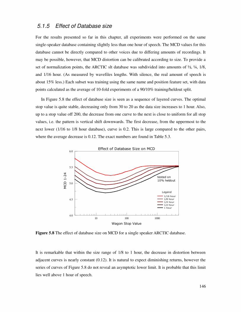
5.1.5 Effect of Database size

For the results presented so far in this chapter, all experiments were performed on the same

single-speaker database containing slightly less than one hour of speech. The MCD values for this

database cannot be directly compared to other voices due to differing amounts of recordings. It

may be possible, however, that MCD distortion can be calibrated according to size. To provide a

set of normalization points, the ARCTIC slt database was subdivided into amounts of ½, ¼, 1/8,

and 1/16 hour. (As measured by wavefiles lengths. With silence, the real amount of speech is

about 15% less.) Each subset was training using the same name and position feature set, with data

points calculated as the average of 10-fold experiments of a 90/10% training/heldout split.

In Figure 5.8 the effect of database size is seen as a sequence of layered curves. The optimal

stop value is quite stable, decreasing only from 30 to 20 as the data size increases to 1 hour. Also,

up to a stop value off 200, the decrease from one curve to the next is close to uniform for all stop

values, i.e. the pattern is vertical shift downwards. The first decrease, from the uppermost to the

next lower (1/16 to 1/8 hour database), curve is 0.2. This is large compared to the other pairs,

where the average decrease is 0.12. The exact numbers are found in Table 5.3.

Figure 5.8 The effect of database size on MCD for a single speaker ARCTIC database.

It is remarkable that within the size range of 1/8 to 1 hour, the decrease in distortion between

adjacent curves is nearly constant (0.12). It is natural to expect diminishing returns, however the

series of curves of Figure 5.8 do not reveal an asymptotic lower limit. It is probable that this limit

lies well above 1 hour of speech.

146

tested on

10% heldout

Wagon Stop Value

10 100 1000

MCD 1-24

4.0

4.5

5.0

5.5

6.0Effect of Database Size on MCD

Legend

1/16 hour

1/8 hour

1/4 hour

1/2 hour

1 hour

number of

utterances

wavefile

size (h)

amount of

speech (h)

stopval = 20

MCD ∆ MCD

77 1/16 0.0546 5.2577 ––

154 1/8 0.1098 5.0565 0.2012

311 1/4 0.2173 4.9518 0.1047

607 1/2 0.4333 4.8199 0.1319

1132 1 0.8116 4.7023 0.1176

Table 5.3 Change in MCD as the size of the database doubles. In computing the

amount of speech present (third column), all silence and pauses are excluded

form the summation. The MCD numbers pertain to a stop value of 20, which is

near-optimal for the conditions trained.

5.2 MCD-based calibration using English

In general, the purpose of calibrating an instrument (such as a weight scale or a voltmeter) is to

adjust the output function to match a known external standard. For speech synthesis, we are

lacking an external standard to begin with. While MCD can be measured, when changing

speakers or crossing languages, the comparison of numbers becomes unclear. Given a measured

distortion of say, 5.15, does this number reflect a good quality voice, or a poor voice? A set of

calibration marks can potentially allow one to make such an assessment. Thus we may ask the

following two questions.

Can an objective measure of MCD be converted into a judgment about whether a voice is

“good” or “bad”?

Can this information be used to advise the user? That is, to suggest a course of action that

will most rapidly improve the voice, e.g. record more speech or verify lexical entries.

Being able to guide or offer advice to the user is the ultimate payoff. We know from section 4.1 at

what rate (one particular) voice improves as the amount of speech is increased. We also need to

know how the voice responds when work is spent on that other major component – the lexicon.

At what rate does a voice improve as the pronunciation lexicon is expanded?

How does this rate compare to collecting more speech?

Is is more important to work on the lexicon or to collect more speech?

147

We can make progress in answering these questions by isolating the effect that the lexicon plays

in voice quality. The basic expectation is that the distortion of a voice will decrease as the

coverage and accuracy of its lexicon improves.

5.2.1 Effect of not having a lexicon for English

The information of Figure 5.8 provides data how how a voice improves with increasing amounts

of speech. The voices in those experiments were constructed with CMUDICT [42] providing full

coverage of the vocabulary. To assess the extent of influence of the lexicon, we replace it with a

crude approximation: using a character-based voice. In a pure grapheme-based voice the

“pronunciation dictionary” is the lexicographic transcription itself. In the following experiments

we consider the voice character-based on account of removing punctuation and reducing letters to

a single case. Thus the phoneset consists of the 26 letters a-z.

The motive of using a character-based voice for calibration is two-fold. First is that it mimics

the voice creation experience of a person using the SPICE tools, who begins with a possibly

faulty phoneme set, records some speech, and builds up the lexicon one word at a time. The

second is that the voice should be substantially inferior, due to the highly irregular spelling

system of English. Such a voice is trained on a large percentage of mis-pronunciations. Hence,

the MCD curve for a character-based voice can be considered a generous upper bound on MCD

distortion.

Figure 5.9 Curves of character-bases versus phoneme-based English voices, built from 1 hour of

speech. The difference in MCD at a stop value of 20 is 0.268.

148

Wagon Stop Value

10 100 1000

MCD 1-24

4.5

5.0

5.5

6.0Grapheme versus Phoneme-based Voices

arctic_slt

Legend

grapheme based

phoneme based

Figure 5.9 compares the MCD curve of the character-based voice (top line) with a phoneme-

based voice (lower curve of Figure 5.8). It came as a surprise that the separate between the curves

is nearly constant. At a stop value of 10 the difference is 0.261, at 20 it is 0.268, at 100 it is 0.262,

and at 800 it is 0.281. Overall, correcting the phoneme set and lexicon decreases MCD by 0.27. It

is reasonable to believe that the average vertical gap is a language-dependent attribute. A

language with a regular writing system, such as Spanish, will exhibit a narrower gap.

The utility of these two curves is that represent a “good” voice and a “bad” voice. They

provide a pair of calibration references against which non-English languages may be compared.

This is taken up in the following section. The question of effort allocation – the relative

effectiveness of recording more speech versus refining the lexicon – is treated in section 4.6.

5.2.2 Evaluating languages other than English

The best form of evaluation is via large-scale listening tests such as is conducted during the

Blizzard Challenge events [29]. While it is crucial to have SPICE users listen to their voice

during development (e.g. transcription of unseen sentences), it is also valuable to apply an

automated means of evaluation. To examine this idea we selected a suite of eight test languages:

French, German, Tamil, Hindi, Bulgarian, Mandarin, Vietnamese and Konkani. Data for these

languages was provided by students working with the SPICE tools, though the voices were rebuilt

for this study. Each is trained from 90% of the available data and tested on the residual 10%.

The results are presented by placing them in the context of the English calibration lines.

Figure 5.10 plots the MCD distortion of each, along with the curves for the character-based and

grapheme-based English voices. In this plot the x-axis is database size (on a log scale), with the

amount of speech with silence frames removed.

149

Figure 5.10 Eight languages placed in context of the bounds of a grapheme-based (upper line)

and a phoneme-based English voice (lower line).

In informal review with the developers, the voices for Vietnamese, Konkani, and Mandarin were

deemed to be poor. French, German, and Tamil were deemed good. Hindi and Bulgarian behaving

acceptably within-domain but not so well out of domain. These assessments are generally

consistent with the above picture. That Hindi and Tamil measured below 5.0 is somewhat

surprising. While the grapheme-to-phoneme relation of these languages is comparatively

straightforward, the low distortion is likely due to their limited domain of application. The 10%

heldout sentences contained phrases present in the training data, and so do not thoroughly

exercise the voice.

To establish a more quantitative assessment of intelligibility, we chose two of the better

synthesizers for listening tests: those of German and Hindi. Twenty sentences were randomly

selected from within the application domain and synthesized, with an additional four extracted

from out of domain. These were presented to testers who were asked to transcribe the words.

They were allowed to listen to the synthesized sentences more than once, and to note which

words became more clear after multiple listening. Transcripts were double-check for typographic

errors. The German listener was the German voice developer and was familiar with the domain.

The Hindi listener was not the developer and thus was not familiar with the domain.

For the German in-domain sentences, 76% of the words were transcribed correctly, versus

55% for the out-of-domain. For Hindi the corresponding rates are nearly identical: 76% and 59%.

This is probably a coincidence. The scores of each utterances are tabulated in the tables below.

150

Database Size (h)

0.1 1

MCD 1-24

4.5

5.0

5.5

6.0Effect of Database Size on MCD - Multi-Lingual

Konkani

Mandarin

Bulgarian

HindiTamil

German

French

VietnameseLegend

character-based

phoneme-based

words correct (German)

1-4 5-8 9-12 13-16 17-20 21-24

3/5 7/8 8/8 4/5 8/8 9/11

1/6 6/8 3/6 3/6 6/7 5/9

4/6 2/8 5/6 3/5 8/9 5/11

8/8 4/6 7/7 9/9 6/7 3/9

overall 105 / 138 22 / 40

Table 5.4 Word transcription accuracy for 24 German test

sentences. Sentences 1-20 are in-domain, while 21-24 are out-

of-domain sentences.

words correct (Hindi)

7/7 6/6 4/8 6/6 4/4 4/6

4/6 5/12 3/5 9/11 5/6 0/6

10/10 3/7 5/8 4/6 6/7 4/5

10/11 7/7 5/8 5/7 2/3 5/5

overall 110 / 145 13 / 22

Table 5.5 Transcription accuracy for 24 Hindi test sentences.

Sentences 1-20 are in-domain; 21-24 are out-of-domain.

A 25% word error rate is respectable for voices built from less than 15 minutes of speech, but is

insufficient for practical usage. This observation raises a critical question. How can an existing

voice be most efficiently improved? The calibration lines of Figure 5.10 provide an easy,

approximate answer. Examining the suite of eight test languages, the French voice is already in

good shape. The German voice could use an improved lexicon. Hindi and Tamil could benefit

from additional speech data. Mandarin, Konkani, and Bulgarian need more data and better

lexicons. Finally, Vietnamese, the outlier, needs to be examined to be checked that there is not a

configuration problem with the software.

Having such calibration lines provides a second – perhaps even more important – benefit: that

of motivation. If a user wishes to devote the energy required for a quality result, they will be

spending multiple days on voice development. At the end of each session there will be a snapshot

that captures the current state. The corresponding MCD can be measured and plotted in a graph

similar to Figure 4.7, and presented to the user as a summary of progress. After each session the

point should move to the right and down, as the voice improves.

151

5.3 Iterative voice development

The English recipe synthesizer was built incrementally in five stages, with recording and lexicon

construction as interleaved tasks. The effort required 2 hours to record one thousand short

utterances plus 2.5 hours to build up the lexicon (tallying only on-task time). The voice from the

previous stage is used to assist creation of the next voice. This is unique to our approach and is

achieved by providing alternate synthesized pronunciations of the word list.

number of time (mm:ss)

utts words tokens recorded wavefiles speech

200 475 1363 25: 11:16 7:45

400 685 2740 47: 21:44 14:48

600 849 4085 70: 32:17 21:50

800 958 5424 95: 42:56 28:59

1000 1057 6776 120: 53:43 36:13

Table 5.6 Size and recording time of prompts.

lexicon words time (mm:ss) coverage

stage total stage total prompts corpus

104 104 20:40 20:40 71.44 46.07

140 244 28:55 49:35 83.74 54.2

193 437 31:10 80:45 91.41 60.97

217 654 26:01 106:46 95.56 67.96

310 964 41:23 148:09 100 73.86

Table 5.7 Five iteration of lexicon expansion on the English test.

The seed lexicon of 394 words is not included.

all words selected type-in corrected

count seconds count seconds count seconds

104 11.8 70 9.8 34 15.9

140 12.4 91 10.1 49 16.7

193 9.7 124 7.2 68 14.4

217 7.2 161 4.7 56 14.4

310 8.0 208 5.9 102 12.3

Table 5.8 For each lexicon building stage, the average time spent

selecting or typing in a pronunciation.

152

The system orders lexical entries to be worked on from the most frequently occurring to the least.

One may take the frequency counts from either the prompt list or from the larger corpus.

Covering all the words in the prompt list first optimizes model building (because the transcript

will be better). Ordering words from the corpus optimizes coverage of the language domain, at

the expense of poorer acoustic models.

Figures Figure 3.24 and Figure 3.25 of Chapter 3 compare three word selection strategies.

They are:

1. prompts before corpus,

2. corpus before prompts, and

3. one from each alternately.

In this experiment we adopted strategy number 1. That is, we first seek a pronunciation for each

word in the prompt list.

When working on the lexicon, each word is accompanied by up to four alternate

pronunciations displayed as a phoneme string. The interface is very similar to that of Figure 4.4

(page 103) used for the development of an Iraqi Arabic lexicon. Each is synthesized using the

voice from the previous stage. We recorded the time required for a native speaker to verify each

word, and how often the wavefiles were played. In Table 5.8 above the average time spent on a

word ranges from 17s to 5s. In difficult cases wavefiles are played eight times or more (Figure

5.11), but most often only once is required. The average number of plays ranged from 3.7 (stages

1 and 2) to 1.8 (stage 4). Table 5.9 shows how often each alternate was chosen when no

corrections had to be made. By design the most probable pronunciation is listed first.

distribution of pronunciation selections

stage 1st 2nd 3rd 4th % 1st

1 54 9 5 2 77.1

2 61 17 12 1 67.0

3 93 27 2 2 75.0

4 132 18 4 7 82.0

5 155 26 22 5 74.5

Table 5.9 For each lexicon building stage, distribution of selection

choices when the pronunciation is taken from the prediction list.

153

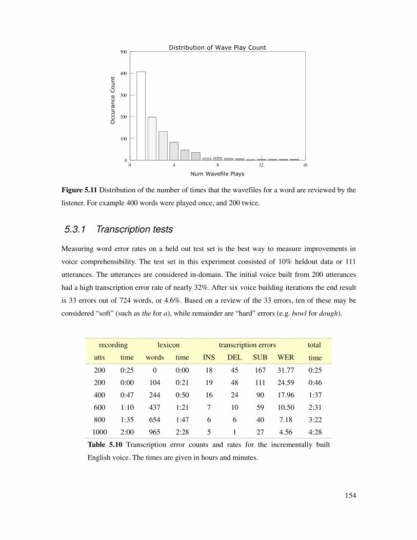
Figure 5.11 Distribution of the number of times that the wavefiles for a word are reviewed by the

listener. For example 400 words were played once, and 200 twice.

5.3.1 Transcription tests

Measuring word error rates on a held out test set is the best way to measure improvements in

voice comprehensibility. The test set in this experiment consisted of 10% heldout data or 111

utterances. The utterances are considered in-domain. The initial voice built from 200 utterances

had a high transcription error rate of nearly 32%. After six voice building iterations the end result

is 33 errors out of 724 words, or 4.6%. Based on a review of the 33 errors, ten of these may be

considered “soft” (such as the for a), while remainder are “hard” errors (e.g. bowl for dough).

recording lexicon transcription errors total

timeutts time words time INS DEL SUB WER

200 0:25 0 0:00 18 45 167 31.77 0:25

200 0:00 104 0:21 19 48 111 24.59 0:46

400 0:47 244 0:50 16 24 90 17.96 1:37

600 1:10 437 1:21 7 10 59 10.50 2:31

800 1:35 654 1:47 6 6 40 7.18 3:22

1000 2:00 965 2:28 5 1 27 4.56 4:28

Table 5.10 Transcription error counts and rates for the incrementally built

English voice. The times are given in hours and minutes.

154

Num Wavefile Plays

0 4 8 12 16

Occurance Count

0

100

200

300

400

500Distribution of Wave Play Count

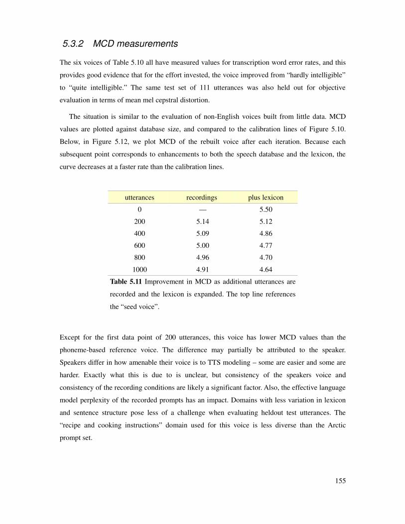
5.3.2 MCD measurements

The six voices of Table 5.10 all have measured values for transcription word error rates, and this

provides good evidence that for the effort invested, the voice improved from “hardly intelligible”

to “quite intelligible.” The same test set of 111 utterances was also held out for objective

evaluation in terms of mean mel cepstral distortion.

The situation is similar to the evaluation of non-English voices built from little data. MCD

values are plotted against database size, and compared to the calibration lines of Figure 5.10.

Below, in Figure 5.12, we plot MCD of the rebuilt voice after each iteration. Because each

subsequent point corresponds to enhancements to both the speech database and the lexicon, the

curve decreases at a faster rate than the calibration lines.

utterances recordings plus lexicon

0 –– 5.50

200 5.14 5.12

400 5.09 4.86

600 5.00 4.77

800 4.96 4.70

1000 4.91 4.64

Table 5.11 Improvement in MCD as additional utterances are

recorded and the lexicon is expanded. The top line references

the “seed voice”.

Except for the first data point of 200 utterances, this voice has lower MCD values than the

phoneme-based reference voice. The difference may partially be attributed to the speaker.

Speakers differ in how amenable their voice is to TTS modeling – some are easier and some are

harder. Exactly what this is due to is unclear, but consistency of the speakers voice and

consistency of the recording conditions are likely a significant factor. Also, the effective language

model perplexity of the recorded prompts has an impact. Domains with less variation in lexicon

and sentence structure pose less of a challenge when evaluating heldout test utterances. The

“recipe and cooking instructions” domain used for this voice is less diverse than the Arctic

prompt set.

155

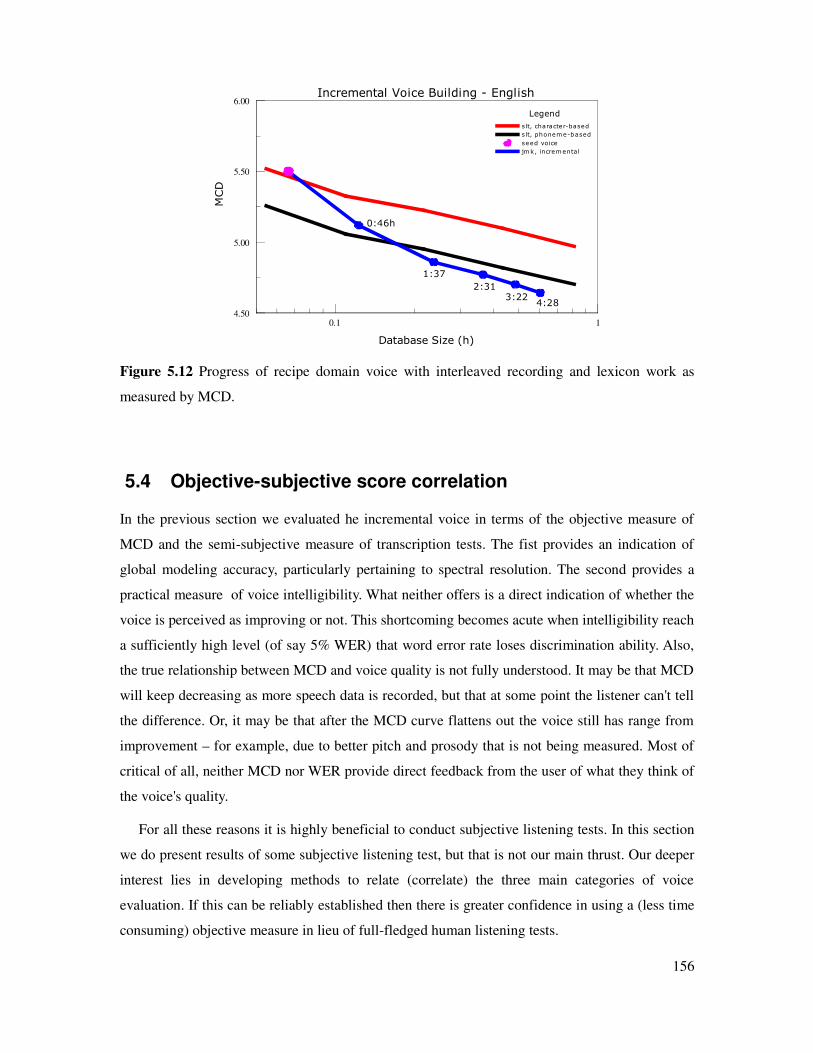
Figure 5.12 Progress of recipe domain voice with interleaved recording and lexicon work as

measured by MCD.

5.4 Objective-subjective score correlation

In the previous section we evaluated he incremental voice in terms of the objective measure of

MCD and the semi-subjective measure of transcription tests. The fist provides an indication of

global modeling accuracy, particularly pertaining to spectral resolution. The second provides a

practical measure of voice intelligibility. What neither offers is a direct indication of whether the

voice is perceived as improving or not. This shortcoming becomes acute when intelligibility reach

a sufficiently high level (of say 5% WER) that word error rate loses discrimination ability. Also,

the true relationship between MCD and voice quality is not fully understood. It may be that MCD

will keep decreasing as more speech data is recorded, but that at some point the listener can't tell

the difference. Or, it may be that after the MCD curve flattens out the voice still has range from

improvement – for example, due to better pitch and prosody that is not being measured. Most of

critical of all, neither MCD nor WER provide direct feedback from the user of what they think of

the voice's quality.

For all these reasons it is highly beneficial to conduct subjective listening tests. In this section

we do present results of some subjective listening test, but that is not our main thrust. Our deeper

interest lies in developing methods to relate (correlate) the three main categories of voice

evaluation. If this can be reliably established then there is greater confidence in using a (less time

consuming) objective measure in lieu of full-fledged human listening tests.

156

Database Size (h)

0.1 1

MCD

4.50

5.00

5.50

6.00Incremental Voice Building - English

4:283:22

2:31

1:37

0:46h

Legend

s lt, character-based

slt, phoneme-based

seed voice

jmk, incremental

5.4.1 A-B preference tests

As discussed in the opening of this chapter, the two predominant choices for subjective listening

tests are absolute-scale estimation and paired-comparison decisions – otherwise known as MOS

tests and AB tests. In this effort we adopt AB tests, for a number of reasons. Primary is that the

listener is asked a simple question of preference. The person making the evaluation does not have

to contend with placing a wavefile heard in isolation onto a 5-point Lickert scale, as is the case

with MOS tests. It is commonly believed that choosing among two alternatives is an easier task

for humans to perform, and thus more accurate. Another advantage of AB tests is that the results

are not bounded to a small closed range, which can suffer from compression effects. There can be

an unbounded chain of “A is better than B is better than C is better than D... and so on” without

concern of running out of headroom.

Figure 5.13 is our user interface for conducting AB tests. (More precisely AB-tie since ties are

permitted.) When using this program listeners process about four utterance pairs per minute. This

is generally faster than placing items on an 5-point scale in a MOS test.

listener pairs per minute

subject 1 3.22

subject 2 4.62

subject 3 3.91

subject 4 4.61

subject 5 3.99

average 4.07

Table 5.12 Average time take to perform

AB-tie listening tests, with the number of

pairs evaluated by each listener not less

than 100.

Figure 5.13 User interface of AB-tie listening tests.

157

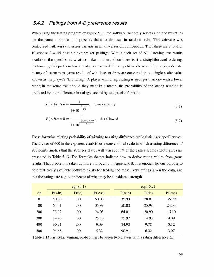
5.4.2 Ratings from A-B preference results

When using the testing program of Figure 5.13, the software randomly selects a pair of wavefiles

for the same utterance, and presents them to the user in random order. The software was

configured with ten synthesizer variants in an all-versus-all competition. Thus there are a total of

10 choose 2 = 45 possible synthesizer pairings. With a such set of AB listening test results

available, the question is what to make of them, since there isn't a straightforward ordering.

Fortunately, this problem has already been solved. In competitive chess and Go, a player's total

history of tournament game results of win, lose, or draw are converted into a single scalar value

known as the player's “Elo rating.” A player with a high rating is stronger than one with a lower

rating in the sense that should they meet in a match, the probability of the strong winning is

predicted by their difference in ratings, according to a precise formula.

P A beats B=1

110−r a−rb

400

, win/lose only(5.1)

P A beats B=1

110−r a−rb100

400

, ties allowed(5.2)

These formulas relating probability of winning to rating difference are logistic “s-shaped” curves.

The divisor of 400 in the exponent establishes a conventional scale in which a rating difference of

200 points implies that the stronger player will win about ¾ of the games. Some exact figures are

presented in Table 5.13. The formulas do not indicate how to derive rating values from game

results. That problem is taken up more thoroughly in Appendix B. It is enough for our purpose to

note that freely available software exists for finding the most likely ratings given the data, and

that the ratings are a good indicator of what may be considered strength.

eqn (5.1) eqn (5.2)

∆r P(win) P(tie) P(lose) P(win) P(tie) P(lose)

0 50.00 .00 50.00 35.99 28.01 35.99

100 64.01 .00 35.99 50.00 25.98 24.03

200 75.97 .00 24.03 64.01 20.90 15.10

300 84.90 .00 25.10 75.97 14.93 9.09

400 90.91 .00 9.09 84.90 9.78 5.32

500 94.68 .00 5.32 90.91 6.02 3.07

Table 5.13 Particular winning probabilities between two players with a rating difference ∆r.

158

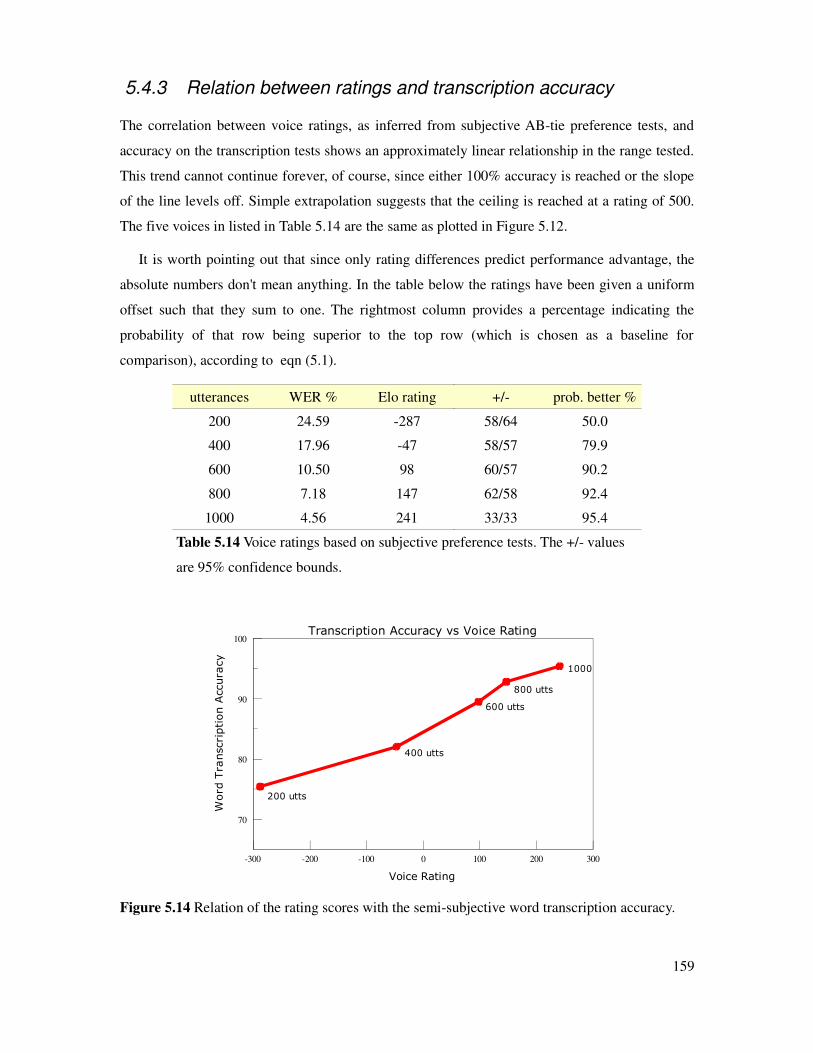
5.4.3 Relation between ratings and transcription accuracy

The correlation between voice ratings, as inferred from subjective AB-tie preference tests, and

accuracy on the transcription tests shows an approximately linear relationship in the range tested.

This trend cannot continue forever, of course, since either 100% accuracy is reached or the slope

of the line levels off. Simple extrapolation suggests that the ceiling is reached at a rating of 500.

The five voices in listed in Table 5.14 are the same as plotted in Figure 5.12.

It is worth pointing out that since only rating differences predict performance advantage, the

absolute numbers don't mean anything. In the table below the ratings have been given a uniform

offset such that they sum to one. The rightmost column provides a percentage indicating the

probability of that row being superior to the top row (which is chosen as a baseline for

comparison), according to eqn (5.1).

utterances WER % Elo rating +/- prob. better %

200 24.59 -287 58/64 50.0

400 17.96 -47 58/57 79.9

600 10.50 98 60/57 90.2

800 7.18 147 62/58 92.4

1000 4.56 241 33/33 95.4

Table 5.14 Voice ratings based on subjective preference tests. The +/- values

are 95% confidence bounds.

Figure 5.14 Relation of the rating scores with the semi-subjective word transcription accuracy.

159

Voice Rating

-300 -200 -100 0 100 200 300

Word Transcription Accuracy

70

80

90

100Transcription Accuracy vs Voice Rating

200 utts

400 utts

600 utts

800 utts

1000

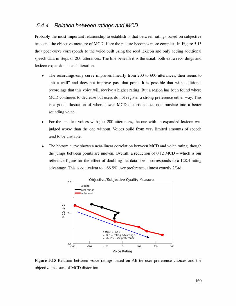
5.4.4 Relation between ratings and MCD

Probably the most important relationship to establish is that between ratings based on subjective

tests and the objective measure of MCD. Here the picture becomes more complex. In Figure 5.15

the upper curve corresponds to the voice built using the seed lexicon and only adding additional

speech data in steps of 200 utterances. The line beneath it is the usual: both extra recordings and

lexicon expansion at each iteration.

The recordings-only curve improves linearly from 200 to 600 utterances, then seems to

“hit a wall” and does not improve past that point. It is possible that with additional

recordings that this voice will receive a higher rating. But a region has been found where

MCD continues to decrease but users do not register a strong preference either way. This

is a good illustration of where lower MCD distortion does not translate into a better

sounding voice.

For the smallest voices with just 200 utterances, the one with an expanded lexicon was

judged worse than the one without. Voices build from very limited amounts of speech

tend to be unstable.

The bottom curve shows a near-linear correlation between MCD and voice rating, though

the jumps between points are uneven. Overall, a reduction of 0.12 MCD – which is our

reference figure for the effect of doubling the data size – corresponds to a 128.4 rating

advantage. This is equivalent to a 66.5% user preference, almost exactly 2/3rd.

Figure 5.15 Relation between voice ratings based on AB-tie user preference choices and the

objective measure of MCD distortion.

160

Voice Rating

-300 -200 -100 0 100 200 300

MCD 1-24

4.5

5.0

5.5Objective/Subjective Quality Measures

Legend

recordings

+ lexicon

∆ MCD = 0.12

= 128.4 rating advantage= 66.5% user preference

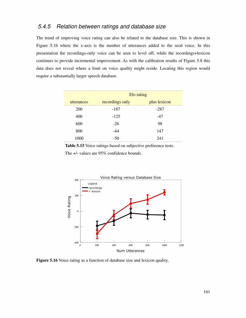
5.4.5 Relation between ratings and database size

The trend of improving voice rating can also be related to the database size. This is shown in

Figure 5.16 where the x-axis is the number of utterances added to the seed voice. In this

presentation the recordings-only voice can be seen to level off, while the recordings+lexicon

continues to provide incremental improvement. As with the calibration results of Figure 5.8 this

data does not reveal where a limit on voice quality might reside. Locating this region would

require a substantially larger speech database.

Elo rating

utterances recordings only plus lexicon

200 -187 -287

400 -125 -47

600 -26 98

800 -44 147

1000 -50 241

Table 5.15 Voice ratings based on subjective preference tests.

The +/- values are 95% confidence bounds.

Figure 5.16 Voice rating as a function of database size and lexicon quality.

161

Num Utterances

0 200 400 600 800 1000 1200

Voice Rating

-400

-200

0

200

400Voice Rating versus Database Size

Legend

recordings

+ lexicon

5.4.6 Best use of effort – larger lexicon or more speech?

In light of the points made in the previous section, one can identify in Figure 5.16 three distinct

domains, or stages of what might be called “recommended user activity.” They are:

1. Initial recording: gathering addition speech without working the lexicon. In particular,

the region from 200 to 600 utterances.

2. Initial lexicon development: fixing the speech database at 600 utterances while expanding

the lexicon. That is, moving vertically along the y-axis to the point above.

3. Interleaved development: recording a batch of 200 utterances, then 200 words to the

lexicon. This is the right side branch of the upper curve.

Based upon the measurement of this experiment, rate of improvement of the voice can be

calculated for each of the above three stages of development.

stage ∆t (min) ∆ MCD ∆ MCD / hour ∆ rating ∆ rating / hour

1 45 .137 .183 161 214.7

2 81 .230 .170 124 91.9

3 117 .128 .066 143 73.3

Table 5.16 Improvement in MCD and voice rating per hour, for the three distinct stages

of recommended development: i) initial recording, ii) initial lexicon expansion, iii)

interleaved voice building.

It is an unfortunate fact that the rate of improvement decreases as the voice becomes more

mature. This is not unexpected, given that the previously found reduction in MCD of 0.12 per

doubling of the database size implies a logarithmic dependence on recording time. From the

perspective of the end user, though, what is encouraging is that the voice improves most rapidly

when it is small. Moreover, we can stipulate a recommended program of action. In simple terms it

is: record first, expand the lexicon second, then do both in turns. The exact transition points will

vary depending on the language being developed and the size of the lexicon required. A useful

guideline is 500-600 initial sentence-length utterances, followed by 500-600 lexical entries.

162

5.5 Summary

In this chapter we have exhaustively analyzed the efficacy and stability of the CART tree training

features employed in voice building. This has allowed us to identify a minimally sufficient feature

set, and to place useful bounds on aspects such as context width. This investigation also

established the promising result that so-called language-independent features achieve 95% of the

modeling potential.

This was followed by extensive experiments on a carefully recorded reference English voice

(Arctic slt). These experiments allow us to calibrate the objective measure of mean mel cepstral

distortion, or MCD. A consistent trends was discovered indicating a log-linear relationship

between MCD and the speech database size. If we call the speech recordings S, then

MCD= 0.12 log2

∣S 2∣

∣S1∣(5.3)

The calibration of MCD using Arctic slt then permitted an evaluation of eight non-English

voices built from small amounts of data. Two of the better voices (German and Hindi) were

further evaluated with transcription tests on held out sentences.

The desire to continue to improve a voice built form limited data led to experiments in

iterative voice building, where the tasks of recording, lexical development, and voice testing are

interleaved in manageable sized chunks of about 20 minutes each. This provided ten voices to

evaluate with respect to subjective, semi-subjective, and objective measures.

Next we introducing the methodology of Elo Rating systems to convert AB paired comparison

choices into scalar rating numbers. This provided the connection sufficient to tie together MCD

and transcription error rates to the subjective evaluation of AB preference choices. According to

our measurements we are able to suggest a new quantitative relation

MCD= 0.12 ⇒ r=128 ⇒ ProbA preferred to B=66% (5.4)

These measures of improvement in quality then allow one to calculate how much a voice

improves per hour of invested time. We also identified some potential pitfalls, such as working on

the lexicon when the voice is too small. Together, these measurements and observations lead to a

recommended procedure for developing speech synthesizers in new languages from zero.

163

164

6 Pronunciations From Acoustics

Having addressed many of the impediments to bootstrapping TTS for new languages, the largest

remaining obstacle is the phoneme set. The objective is to dissolve the user of responsibility of

knowing the phoneme set for their language. The work of this chapter explains how to iteratively

evolve a phoneset appropriate for TTS, to adjust it accordingly as the phoneset evolves, and to

learn a lexicon on the basis of acoustic evidence. The user steers the learning process by

providing pronunciation feedback, but is relieved of explicitly defining a phoneset and building a

lexicon.

Bootstrapping TTS from Zero requires a recognizer and synthesizer as supporting functional

components. They are initialized either from a provided (if approximate) phoneset if one exists,

or lacking that, from the grapheme set. During the lexicon inference stage, the recognizer is used

to suggest hypothesis pronunciations by performing phoneme decoding on the speech corpus. The

suggested pronunciations are synthesized using the current iteration of the synthesizer. The

synthesized wavefiles are measured the original. For a given word or sentence, hypothesis that

generates the minimum distortion wavefile is deemed to provide the best pronunciation. This

synthesizer-centric approach to pronunciation is novel to this thesis, and makes perfect sense

when the ultimate objective is a speech synthesizer. We are not attempting to infer pronunciations

that maximizes the likelihood of the data given the HMM acoustic models, or that lower the word

error rates of a decoder. An ASR-centric approach is fine when it is the component being

optimized. In this thesis, ASR plays a vital yet supporting role.

Section 6.1 presents the inference algorithms, beginning with a definition of terms. Then in 6.2

we address the problem of inferring pronunciations of words from their acoustics, without human

intervention. Section 6.3 describes the way in which an initial phoneset is progressively split and

merged to create an improved base of support for synthesizer training. This is a procedure of

165

“phoneset purification.” Ina simplified implementation of phoneset purification is illustrated in

the purely symbolic realm of graphemes and phonemes. Section 6.4 uses the English Arctic

databases to exemplify the process of lexicon inference for a mature. That is, where the phoneme

set is well established and there is an existing lexicon, but one wants to verify the lexicon using

spoken samples. Also, the amount of speech available is large (over two hours), which allows us

to perform experiments and draw conclusions without concerns of lack a data.

6.1 Automatic lexicon inference – description

Building TTS from zero involves an iterative procedure. It is iterative in two regards. One, with a

human in the loop it is advantageous to incrementally add speech and provide corrective feedback

– as presented in Chapter 5. Two, if the starting point is an approximate phoneme set, or if the

phoneme set is initialized with graphemes, then the initial models will be sub-optimal.

Optimizing the phoneset, lexicon, and speech models is most easily accomplished through

incremental improvements. The purpose of this section is to decompose the procedure into a

series of smaller steps.

Iteration occurs at multiple levels, or layers. The work of Chapter 5 belongs to the outermost

layer: where the user records speech in manageable batches, interleaved with lexical corrections

and transcription tests. At this layer, the working phoneset is fixed. Changes to the phoneset occur

at the next layer down, where either two similar phones are merged together, or an impure phone

is split apart. Below this level the lexicon is automatically refined on the basis of acoustic

evidence. When the lexicon is changed the speech models are retrained accordingly.

1. Outer layer – incremental addition of speech and user feedback.

2. Middle layer – automatic refinement of phoneset.

3. Inner layer – automatic refinement of lexicon.

4. Model layer – retraining of ASR acoustic model and TTS voice model.

At the model layer, the retraining of ASR and TTS components is performed through existing

techniques, such as Baum-Welch acoustic model training. Our attention is directed towards the

layers above.

166

6.1.1 Definition of Terms

The full system may be decomposed into five main components. First, there is input Data, Din .

This includes a corpus of speech data and corresponding transcript, the lexicon implicit in the

transcript, and so forth. The data may be collected incrementally, with the user recording chunks

of speech in a sequence of sessions. A collection of Trainers converts the data into Models.

Specifically these are Acoustic Models and Language Models for ASR, Voice Models for TTS,

and G2P models to convert text into phonetic transcription. Each model has a corresponding

training component. The models themselves do not alone comprise the recognizer or synthesizer.

These are grouped under the term Generators. Generators are the converse of Trainers – they use

the models to generate data, Dout , i.e. text from a recognizer and wavefiles from a synthesizer.

Finally, Scorers are functions that operate on the output of Generators. Their purpose is to

evaluate the goodness of the output data. One scorer used to evaluate synthesizer quality is MCD

(mean mel cepstral distortion), as discussed previously in Chapter 5. Scorers can also be humans

– that is, users who participate in listening tests. This information can then be incorporated into an

updated build of the total system.

By convention, models individual are represented by lambda λ, and a group of models by

capital lambda Λ. The scorers are given by phi, Φ.

System = (D, T, Λ, G, Φ) = (Data, Trainers, Models, Generators, Scorers) (6.1)

T : Din (6.2)

G : Dout (6.3)

: DoutDin (6.4)

6.1.1.1 Data Components

This subsection specifies the data components in greater detail so they they may be referred to

with precision in the algorithm descriptions that follow. The corpus of speech data that the user

records and provides to the system is input data. Synthesizer generated speech is an example of

output data. Other data components such as the transcript are input to the model trainers, but are

also the product of processing on the output side (to generate an updated or refined transcript),

which is then fed back to the input side. Additional data, in particular speech recordings, can be

injected periodically into the process by the user. Periodic injection of data is in contrast to using

a fixed (and large) corpus of text to train an ASR language model. In our experiments the

167

language model created once and held fixed.

As is the convention, O stands for the set of acoustic observations, i.e. the waveform files pre-

processed to cepstral feature files. W is a sequence of words that corresponds to O. To support the

training of our system the speech corpus is divided into two sets. These are a set of continuously

spoken speech, i.e. phrases, sentences, paragraphs. The second is a set of discretely spoken

speech, i.e. single words said in isolation, or a sequence of words with substantial pauses between

the words. The purpose of the discrete speech is to provide isolated the pronunciation of words as

spoken in careful form.

O=O c ,Od , O c∩Od=∅ , where (6.5)

Oc≡continuous speech ,i.e. sentences (6.6)

Od≡discrete speech , i.e. isolated words (6.7)

Each of these partitions of the speech data is comprised of individual wavefiles. Let the number

of wavefiles in the continuous and discrete partitions are n, and m. These values can change if the

user records utterances in batches. The number of utterances in the discrete set, m, is independent

of n. However if all words in the prompts are recorded in isolation, then m is the size of the

vocabulary V.

Oc=oc ,1 , oc ,2 ,...oc ,n (6.8)

Od=od ,1 , od , 2 , ...od ,m (6.9)

The continuous speech data is split into training and testing partitions. Typically, the utterances

are separated according to a 90/10 percent split, with the test utterances uniformly sampled from

the time-ordered recording list. A subscript i is used to indicate the iteration number.

Oc , i=O c ,train , i∪O c ,test ,i , O c ,train , i∩Oc , test , i=∅ (6.10)

Each of the recordings in O has a corresponding transcript W.

W i=W c ,i , W d , i=W c , W d i , where (6.11)

Wc ,i=w

c ,1 , wc ,2 , ... w

c ,ni (6.12)

Wd ,i=w

d ,1 ,wd ,2 , ... w

d ,mi (6.13)

Even when the entire speech corpus is processed in one batch (no incremental recording), the

iteration index is needed in equation 6.11. This is due to changing pronunciation variants, which

168

will be reflected in the evolving transcript. To illustrate by way of example, suppose that the first

sentence in the corpus is taken from the Arctic database:

(6.14)

Every word will have a pronunciation listed in the lexicon. What is pertinent is that the lexicon

can list alternate pronunciations for each word, and that the pronunciation assigned to a particular

word in the transcript can change as the data is processed. Thus, the word “the” may have the

three entries /dh iy/, /dh ah/, and /dh ih/. Initially, the default pronunciation /dh iy/ is assigned.

But, suppose after a stage of processing the acoustic evidence suggests the reduced from /dh ah/.

This choice is marked in the transcript text as “the'01”.

(6.15)

The active vocabulary is the union of all the words in the transcript. (Pronunciation variants of the

same orthographic form are treated as one word.)

Vc , i=

w∈W c

VocabWc , i i=iteration number (6.16)

Vd ,i=

w∈W d

VocabWd ,i (6.17)

Vi=

w∈W

Vocab Wi=V

c , i∪V

d ,i (6.18)

∣V i∣≤∣V i1∣ (6.19)

The operator Vocab extracts headwords from the transcript. As an example, if eqn (6.15) were the

entire corpus, Vc,1 = author, danger, etc, of, philips, steels, the, trail. As a matter of practicality,

punctuation and word variant markers are stripped off of headwords. If the speech data being

recorded in multiple sessions the vocabulary will be non-decreasing in size. Similarly, a Charset

operator extracts the characters from the current transcript to define U (“U” for Unicode).

Ui=

w∈W

Charset Wi=U

c , i∪U

d ,i (6.20)

∣U i∣≤∣U i1∣ (6.21)

While not a requirement, it is preferable for the learning algorithm that any vocabulary items in

the discrete data set are also present in the continuous set. That is, the words that the user is asked

to record in isolation are extracted from the continuous speech corpus.

169

wc ,1,1=Author of the'01 danger trail, philip steels, etc.

wc ,1,0=Author of the danger trail, philip steels, etc.

V d⊆V c , U d⊆U c in general (6.22)

V d=V c , U d=U c with full coverage of vocabulary by W d (6.23)

A phoneset is introduced into the model and is denoted by R. There are a number of ways the

phoneset can be introduced. It can be defined by the user, as would is the normal situation in

building speech system. Alternatively, it can be initialed from the character set U. The most

straightforward initialization is to define a one-to-one mapping from every character to a

corresponding phone symbols. Naively, a one-to-one mapping creates a phone symbol for every

punctuation mark in V, as well as all whitespace, but this would violate common sense. More

reasonably, the initialization function maps whitespace and the standard ASCII punctuation marks

to the null, or silence phone SIL. The SIL phone is a pre-defined symbol, along with utterance

start and end markers <s> and </s>. Also, for Western languages, casing in the character set may

be folded together as a practical simplification. The transcript item of eqn (6.14) was stripped of

punctuation and converted to lowercase. By conversion, the corresponding character-initialized

phoneme transcript is uppercase.

(6.24)

The second line of the becomes the first element of Pc, the phonetic transcript corresponding to

Wc. The corresponding Lexicon L0, has a one-to-one form.

author A U T H O R

etc E T C

of O F

...

If the initial phoneset is not character-based (i.e. phonetically defined from an external source),

then the initial lexicon is more traditional.

author AO TH ER

etc EH T S EH T ER AH

of AH V

...

Summarizing, the Data Model D has nine components.

D = (Text corpus, Speech, Word transcript of speech, Character set, Vocabulary,

Phoneset, Phonetic transcript of speech, Phonetic transcript of text, Lexicon)

170

wc ,1,0=author of the danger trail philip steels etc

pc , 1,0=A U T H O R O F T H E D A N G E R T R A I L P H I L I P S T E E L S E T C

D=T ,O ,W ,U , V , R , PO

, PT , L (6.25)

How the model Λ is initialed from D is discussed in the next section, followed by description of

the inference and update algorithms.

6.1.1.2 Model Component Initialization

The system contains four major model components. These are a trigram phone-to-phone

transition probability language model (LM), an HMM-based acoustic model for ASR (AM), a

CART-tree based voice model for TTS (VM), and a grapheme-to-phoneme rule system (G2P).

The language model provides conditional probabilities on a phoneme sequence P pi∣pi−1 , pi−2

and is used by the ASR component to perform phoneme decoding. A word-based language model

is not a part of our system, as bootstrapping TTS does not require a word decoder.

Λ = (Language Model, Acoustic Model, Voice Model, G2P Rules) (6.26)

Λ=LM , AM ,VM ,G2P (6.27)

For model initialization begin with an initial set of recordings O0 selected from the text corpus T,

and corresponding transcript W0 from which the character set and vocabulary is derived.

Charset :T U 0 character set from text (6.28)

Select :T W 0 word transcript from text (6.29)

Record :W 0O0 recorded speech (6.30)

Tokenizer :W 0V 0 vocabulary from transcript (6.31)

Then, as described in the previous section, the initial G2P model is defined – either using an

externally defined phoneset R0, or one that is essentially in a one-to-one correspondence with the

pronounceable characters. The G2P rules are used to map the character set to phones, the

vocabulary to the lexicon, the word transcript to a phonetic transcript, plus the text transcript to a

(distinct) phonetic transcript.

G2P :U 0 R0 phoneset from character set (6.32)

G2P :V 0 L0 lexicon from vocabulary (6.33)

G2P :W 0 P0W phonetization of words (6.34)

171

G2P :T 0P0T phonetization of text (6.35)

From this last transcript a phone-transition language model is learned.

Ngram Learn: P0T LM 0

phone transition language model (6.36)

Below, statistics for two language models trained from the Arctic corpus of 445k sentences are

provided as an example.

tokens types

unigrams sentences unigram bigram trigram

char-based 35,331,847 44791 31 759 13964

phone-based 30,838,426 44796 43 1519 13964

Table 6.1 Language Models built from Arctic text corpus.

Next, in what are well-established training procedures, we build acoustic models for ASR and

voice models for TTS. These models are trained from Oc,train, the continuous speech training

subset of the the initial recordings O0 (as opposed to the discrete words of Od).

ASR Learn :O c ,train , 0 , P0W AM 0

build decoder model (6.37)

TTS Learn :O c ,train , 0 , P0W VM 0

build voice model (6.38)

This completes the construction of the initial models Λ0.

6.1.1.3 Initial Model Testing

With an initial synthesizer built, it undergoes its first evaluation. The 10% heldout test sentences

are resynthesized using the current voice model and lexicon, as per eqn (6.39). Comparison to the

original wavefiles yields an MCD distortion measure, eqn (6.40). If the synthesized sentences are

presented to the user, or to a test subject, human transcriptions can be collected and evaluated to

give a transcription word error rate of eqn (6.41). In the discussion of iterative voice building

(section 5.3) this constituted the first testing stage.

TTS :Oc , test ,0 ,W c ,0, test , L0O c ,syn ,0 synthesize sentences (6.39)

MCD :O c ,test ,0 ,O c , syn ,0MCD0 measure MCD distortion (6.40)

Subj :O c ,syn ,0W syn , 0WER0 measure word error rate (6.41)

172

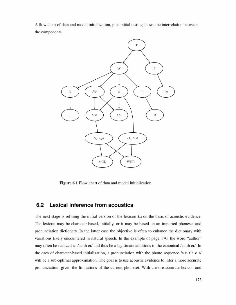
A flow chart of data and model initialization, plus initial testing shows the interrelation between

the components.

6.2 Lexical inference from acoustics

The next stage is refining the initial version of the lexicon L0 on the basis of acoustic evidence.

The lexicon may be character-based, initially, or it may be based on an imported phoneset and

pronunciation dictionary. In the latter case the objective is often to enhance the dictionary with

variations likely encountered in natural speech. In the example of page 170, the word “author”

may often be realized as /aa th er/ and thus be a legitimate additions to the canonical /au th er/. In

the caes of character-based initialization, a pronunciation with the phone sequence /a u t h o r/

will be a sub-optimal approximation. The goal is to use acoustic evidence to infer a more accurate

pronunciation, given the limitations of the current phoneset. With a more accurate lexicon and

173

Figure 6.1 Flow chart of data and model initialization.

MCD

PW

PT

LM

AML

O

VM

WER

R

U

T

W

V

Oc, testOc, syn

transcript, one can then rebuild better acoustic models for decoding and synthesis. With this

motivation the objective is to achieve it with minimal input from the user – i.e. without a large

amount of effort and without great technical expertise.

Inferring pronunciations from acoustics is not a simple matter of running a decoder to

compute the standard formulation argmaxw

P W∣O =P O∣W P W . The main reason is

practical: output from a HMM-based phonetic decoder is highly variable. The variability is

readily established by observing the sensitivity of the output to the relative weighting assigned to

the acoustic model and language model. Part of this variability is due to a mismatch between the

target speaker and the group of speakers used for training (plus differences in acoustic

environment). But even if the training and testing data matched exactly, the decoder is inclined to

de-emphasize the information in the region of phone transitions in favor of the middle of HMM

states. This subtle recognition bias tends to overlook some of the discriminating cues that humans

attend to.

6.2.1.1 Minimum distortion hypothesis as best

In answer to these concerns, our approach reverses the decision process. In almost all previous

work, evaluation of the posterior probability P W∣O is used to determine pronunciations from

acoustics. In contrast, we use the decoder in the role of a hypothesis generator, with the

synthesizer testing the various hypotheses. The synthesizer determines the best one – that is, we

compute the maximum likelihood wavefile P O∣W by means of Festival's maximum likelihood

parameter generation (MLPG) module. Then, instead of invoking Bayes law, the MCD distortion

between the synthesized wavefile and the original is measured. The hypothesis that produces the

minimal distortion wavefile is deemed the best pronunciation.

Should one be unhappy placing total trust in a mathematical measure, MCD can be used to

filter and rank the hypotheses into a short list, which are then presented to the user for review,

similar to the approach of Chapter 4.

Methods for automatic inference of pronunciations can be contrasted with with the assistance

of three questions.

1. How are the hypotheses generated? We use two sources: predictions from G2P rules,

and hypotheses generated from phonetic decoding. These are in addition to any entries of

a given word already present in the lexicon.

2. Spoken context – are the words to be spoken in isolation, or within continuous

174

speech? If the latter, is it read speech or conversational speech? This is a design choice.

Inference from words spoken in isolation reduces effects of coarticulation and reduction

(and so are more careful), but is less likely to reflect typical continuous speech.

3. How are the hypotheses evaluated? This depends on the intended application. If the

application is ASR then it is reasonable to make decisions that directly reduce the word

error rate (discriminative training), or indirectly reduce word error rate by maximizing

the likelihood of the models (EM training). With our emphasis on TTS, minimizing

synthesized distortion is the more appropriate choice.

6.2.2 Inner Iterative Loop – Lexicon update

In brief, our method for updating the lexicon consists of the steps of a) generating hypotheses, b)

synthesizing each of the hypotheses, c) updating the lexicon with the minimal distortion

hypothesis. The three sources for lexical hypotheses are

1. predictions from word orthography using the current G2P rules

2. Viterbi decoding of the speech against the current multi-entry lexicon

3. speech recognition results from a decoder run in phonetic-decoding mode.

The second and third sources use acoustic evidence in different ways. Force alignment finds

the highest likelihood word transcription against a lexicon containing a (typically small) number

of alternate pronunciations. Allphone decoding is constrained, not at the word level, but at the

phonetic level by a phone-transition language model. It offers a “free form” interpretation of the

speech. To extract word pronunciations, the phonetic decoding is DTW aligned to the results of

forced alignment. This procedure is explained in the following section.

The data sets required are the current word transcript, lexicon, language model, and speech. As

mentioned, the G2P rules and AM are used to generated hypothesis. The TTS VM is used to

synthesize the candidates which are compared to the recorded speech. This update algorithm can

be applied to either the discrete speech data Od, or the continuous speech data Oc, or both. In the

following notation only the discrete case (of dictionary words spoken in isolation) is indicated.

G2P :W d , 0 , L0W d , g2p , 1 pronunciation predictions (6.42)

ASR :Od ,0 ,W d , 0 , L0W d ,lex , 1 force aligned transcript (6.43)

ASR :Od ,0 , LM 0Pd ,nbest ,1W decoded nbest transcripts (6.44)

175

DTW :W d ,lex , 1 , Pd , nbest , 1W d , nbest ,1 align word/phone transcripts (6.45)

The transcript from each source are joined, and then filtered to create a final hypothesis list. A

filtering procedure to accept only the top N hypotheses is used to eliminated unlikely candidates.

Filtering can also be a null operation, i.e. allowing every candidate through for testing.

Join :W d , g2p , 1 , W d , lex , W d , nbest , 1W d , comb,1 combine transcripts (6.46)

Filter :W d ,comb ,1W d ,hyp ,1 filter transcripts (6.47)

Extract : L0, W d , hyp ,1 Lhyp ,1 extract lexicon (6.48)

To make the explanation specific, suppose the language is English and the word under

examination is “etc.” – the short form of “etcetera”. For sake of discussion, a modified version of

CMUDICT provides the initial reference pronunciations. The first CMUDICT entry for “etc” is

/eh t s eh t er ah/. The spelled out form of the acronym “E.T.C.” is also valid (/iy t iy s iy/), as is

the fully spoken form “Entertainment Technology Center.” In contrast, the G2P rule system

attempts to pronounce “etc.” as an ordinary word, and comes up with the two predictions /eh t k/

and /ih t k/. These are wrong, but quite reasonable if the string were extracted from a normal word

such as “metcalf” (but not “etch”). Added to these are the output of the phoneme decoder, which

matches none of the above but includes reduced forms such as /ih k s eh t r ah/.

G2P EH T K

IH T K

Dictionary EH T S EH T ER AH

IY T IY S IY

EH N T ER T EY N M AH N T T EH K N AA L AH JH IY S EH N T ER

Decoded IH K S EH T R AH

IH K S AE T R AH

K S EH T R AH

IH K S EH T R AE

...

All of the three dictionary entries are force aligned to the utterance containing the word – wd,0,i for

the discrete recordings and wc,0,i for the continuous recordings. Assuming that the word is spoken

as “etcetera,” during the forced-alignment procedure the first form /eh t s eh t er ah/ is selected

from the set of dictionary-based choices. This selection is taken as the acoustically-derived

dictionary-based reference. This is not necessarily the final, minimum distortion hypothesis.

176

TTS :W d , hyp ,1 , Ld , hyp , 1Od ,hyp ,syn ,1 synthesis of hypotheses (6.49)

MCD :Od , 0 , Od , hyp , syn , 1W d , best , 1 select minimal distortion hyp (6.50)

Extract :W d ,best ,1 L1 extract lexicon (6.51)

Supposing that the first of the decoded pronunciations results in minimal-distortion synthesis, the

lexicon is updated to include this entry. Pre-existing dictionary entries are not removed. Thus the

lexicon now contains four entries for this word.

Dictionary EH T S EH T ER AH

IY T IY S IY

EH N T ER T EY N M AH N T T EH K N AA L AH JH IY S EH N T ER

IH K S EH T R AH

A flowchart of the lexicon update procedure shows the path from L0 to L1.

Figure 6.2 Flow chart of lexicon update procedure.

177

filter

MCD

G2Pdecodefalign

TTS

extract

DTW

Wd, best, 1

Ld, 1

G2P0

Od, hyp, syn, 1

L0

Wd, g2p, 1

Wd, nbest, 1

Wd, lex, 1Pd, nbest, 1

LM0

Wd, hyp, 1

Lhyp, 1

Wd, comb, 1

Lcomb, 1

Wd, 0O0

6.2.2.1 Lexicon inference – discrete-only versus discrete+continuous

With a speech corpus divided into discrete and continuous components there are two main

options for lexicon inference. One may infer word pronunciations from the discrete set only. Or

one may use both sets for inferring word pronunciations. The first option is more constrained in

that pronunciations are learned only from words spoken in isolation, which can be expected to be

carefully spoken speech. When pronunciations are allowed to be learned from the continuously

speech corpus, they can be expected to be more diverse – showing greater variation and deviation

from an initial reference dictionary – but also closer to pronunciation as actually spoken in natural

speech. Learning from both sources exhibits a symmetric structure in the corresponding

flowchart.

Figure 6.3 Flow chart of lexicon update from discrete and continuous data.

In the asymmetrical case of Figure Figure 6.4, decoding the continuous speech corpus

provides ranking information for the pronunciation alternates. The simplest ranking is to count

the number of occurrences of each pronunciation variant found in the entire set of recordings

available at this stage. Ranking by occurrence count is useful for determining the most common

form of frequently spoken words. Though for words where there is only one instance in the

corpus, ranking by occurrence count makes no difference. Results of an experiment illustrating

count-based ranking is provided later in the chapter.

The second purpose of generating an updated word transcript Wc is to provide a more accurate

training transcript for rebuilding acoustic models.

178

Od,0

Wd,1

Ld,1

Wd,0Oc,0

Wc,1

Lc,1

Wc,0 L0

L1

Figure 6.4 Flow chart of lexicon update from discrete speech data only.

6.2.2.2 Word extraction from phonetic decodings

In eqn (6.45) Dynamic Time Warping is applied to find the best alignment between a) the

phonetic decoding of prompts, and b) the corresponding word transcription. This is necessary

because the output of phonetic decoding is a sequence of phones without any indication of word

ownership. However, both the phonetic decoding and the forced alignment to the dictionary-

based transcript provide the time of each respective unit in terms of the segment's ending frame

number. For our purposes, the objective of dynamic time warping is to find the alignment

between words and phones that minimizes the difference in frame numbers.

We illustrate the procedure with an actual example: the short sentence “Will we ever forget

it?” from the beginning of the ARCTIC corpus. In Table 6.2 the word level frames of eqn (6.43)

are aligned to the phone level frames of eqn (6.44), resulting in the pronunciations of Table 6.3.

The word “it” is assigned a new, alternate pronunciation /ae t/. All other word pronunciations

exist in the reference dictionary and are not novel. Note that he sentence termination symbol </s>

picks up the decoding artifact phone /s/, and is discarded (because </s> is not a lexical entry). It is

not unusual for spurious decoded phones appearing at the endpoints to be discarded as part of the

silence section. They can also be (mistakenly) incorporated into the word's pronunciation,

depending on the details of frame alignment.

179

L0

Oc,0

Wd,0

Wd,1

Ld,1

Od,0

Wc,1

Wc,0

L1

“Will we ever forget it?”

word trans. <sil> will we ever forget it </s>

word frames 19 37 61 79 122 147 151

phone frames 16 25 29 35 44 58 64 71 79 92 99 108 117 122 132 138 151

phone decode SIL W IH L W IY EH V ER F ER G EH T AE T S

alignment cost 3 5 8 8 8 17 17

Table 6.2 Word to phone level alignment for extracting pronunciations. Each frame is 10 ms

long, with the utterance 1.51s in length. The symbol <sil> is an inserted silence.

word pronunciation comment

<sil> SIL discarded

will W IH L standard pronunciation

we W IY standard pronunciation

ever EH V ER standard pronunciation

forget F ER G EH T standard pronunciation

it AE T alternate pronunciation

</s> S discarded

Table 6.3 Aligned pronunciations of Table 6.2.

6.2.2.3 Iterative Model Update

With a procedure in place for revising the lexicon and phonetic transcript on the basis of acoustic

evidence, the ASR and TTS models can be retrained. The procedure is iterative, with alternating

passes of lexicon updating and model retraining. The models are considered converged when the

lexicon has stabilized with no changes between iterations, subject to a limit on the iteration count.

In equations 6.52 and 6.53 AM0,i and VM0,i refer to acoustic models trained from the initial (O0)

collection of speech data, after the ith iteration of lexicon updating. Once converged these result

in AM1 and VM1.

ASR Learn :O c ,train , 0 , P0, iW AM 0, i AM 1

converge decoder model (6.52)

TTS Learn :O c ,train , 0 , P0, iW VM 0, iVM 1

converge voice model (6.53)

In the list of page 166, this iterative update procedure is called Inner Loop model refinement.

180

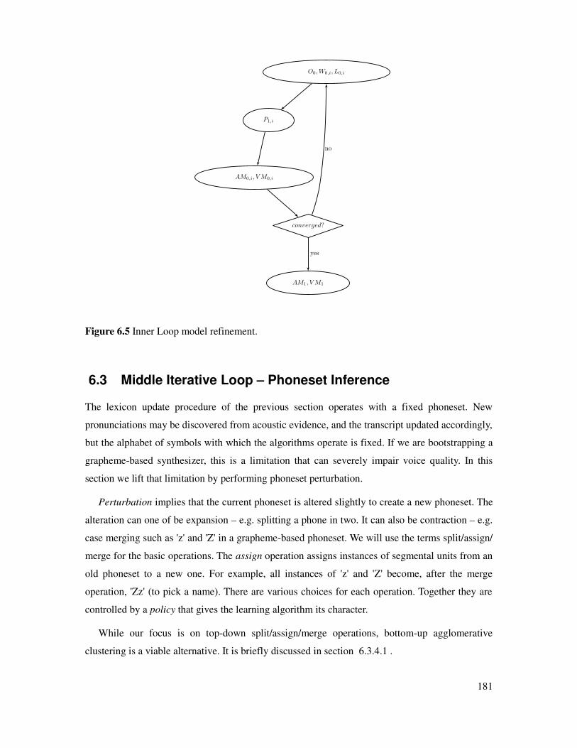
Figure 6.5 Inner Loop model refinement.

6.3 Middle Iterative Loop – Phoneset Inference

The lexicon update procedure of the previous section operates with a fixed phoneset. New

pronunciations may be discovered from acoustic evidence, and the transcript updated accordingly,

but the alphabet of symbols with which the algorithms operate is fixed. If we are bootstrapping a

grapheme-based synthesizer, this is a limitation that can severely impair voice quality. In this

section we lift that limitation by performing phoneset perturbation.

Perturbation implies that the current phoneset is altered slightly to create a new phoneset. The

alteration can one of be expansion – e.g. splitting a phone in two. It can also be contraction – e.g.

case merging such as 'z' and 'Z' in a grapheme-based phoneset. We will use the terms split/assign/

merge for the basic operations. The assign operation assigns instances of segmental units from an

old phoneset to a new one. For example, all instances of 'z' and 'Z' become, after the merge

operation, 'Zz' (to pick a name). There are various choices for each operation. Together they are

controlled by a policy that gives the learning algorithm its character.

While our focus is on top-down split/assign/merge operations, bottom-up agglomerative

clustering is a viable alternative. It is briefly discussed in section 6.3.4.1 .

181

no

yes

P1,i

AM0,i, V M0,i

O0, W0,i, L0,i

converged?

AM1, V M1

6.3.1 Split operations

Given the current phoneset R0, a split operation selects a particular phoneme and divides its

members into two parts. Theoretically the unit could be split into multiple parts, but two is the

minimal perturbation.

Split : R0R1, ∣R1∣=∣R0∣1 split phoneme (6.54)

example : R0 R1=R0−ae ae0, ae1 /ae/ is split

The are numerous ways of choosing a phoneme to split. Here are four possibilities.

1. Split the most commonly occurring phone. This is simplest and a reasonably safe choice.

The downsides are that some popular and uniform sounding phones such as /s/ may split

several times before the difference in sound quality is enough to effect a change in

pronunciation (i.e. be phonemic). Also, there is the threat that a phone split merely on

occurrence count will merge together again during a subsequent merge operation.

2. Split the phone with the largest acoustical variance, according to the AM. This is

mathematically more solid, since the objective is to purify phones exhibiting high

variance in acoustic space. Variance is easiest to compute for HMMs with a single

Gaussian mixture component.

3. Split the highest entropy phoneme according to the confusability matrix. The

confusability matrix counts the number of times phone phi is decoded as phone phj

during the previous lexicon update procedure. This is perhaps the most theoretically

sound choice, since counts of phone substations is a direct measure of pronunciation

irregularity, and hence impurity of the phone class. It is beneficial to weight the entropy

of phone ph with it's probability: Impurity ph = p phH ph . Otherwise, low

frequency phones with few samples may not have enough examples for a reliable

estimate of entropy.

4. If computation efficiency is not a concern, each phone can be split one at a time, then

some measure of the results taken before reverting to the original R0. The highest scoring

candidate is selected for splitting. For example, the CART trees constructed during voice

building are an example of this kind of test-and-decide clustering. In particular the

clusters are predicted from defined features, and the cluster splits are determined by the

greatest reduction in variance. The CART tree learner tests all possible splits, measures

the results, and chooses the most effective split.

182

6.3.2 Assign operations

Once a phoneme has been split, the assignment operation classifies each instance of ph into one

of the two clusters ph0 and ph1.

1. A straightforward approach is to apply k-means clustering on the frames within a phone

segment. This is computationally efficient but does not consider the time-trajectory of a

unit.

2. Gaussian splitting can be applied, as is for example implemented in SphinxTrain. This has

the advantage of evaluating the time-evolution of a segment.

6.3.3 Merge operations

Merge operations may be “hard” or “soft” [102].

1. A hard merge operation joins two phonemes together. All instances of each class are

combined. The two closest phones, according to some measure of inter-class distance, are

merged.

2. An annealing operation, or soft merge, keeps all of the phone classes, but reassigns units

in the continuous corpus as per the lexicon update procedure discussed above. Only when

the count of units in a phone class falls to zero is the class retired from active use.

6.3.4 Split/assign/merge policy

The split/assign/merge policy controls the sequencing of operations. Some examples are:

1. split-split-merge. This grows the phoneset by one unit per cycle. It is appropriate, for

example, to expand an initial grapheme-based phoneset of 26 lowercase ASCII letters to

the 40-50 phonemes of English. The exact number of cycles depends on the dialect and

stopping criteria.

2. merge-merge-split. This shrinks the phoneset by one unit per cycle. It is appropriate for

when the initial phoneset is based on all graphemes, e.g. with case not folded and digits

and punctuation retrained.

3. merge 8 – split 8. This is the policy of [145] and was chosen to compare existing large

and small phonesets used in English ASR systems. The large changes in phoneset size

result in relatively drastic changes to the speech models.

183

4. split-anneal. This is the favored policy. A split is followed by a soft merge operation. This

has the advantage of not making strong assumptions about the relative size of the

grapheme and phoneme sets of a language. In a grapheme-seeded system it is satisfactory

in either an initial under-population or over-population of phone units.

6.3.4.1 Bottom-up agglomerative clustering

The idea regarding phoneset inference has been that the initial phoneset is close in size to what a

linguist would define. When grapheme-based it is generally somewhat smaller. Thus the inference

policy enacts a top-down divisive clustering algorithm. A viable alternative is bottom-up

agglomerative clustering from tri-graphemes [5]. In this approach the initial phoneset consists of

hundreds of tri-graphemes. A tri-grapheme is a letter conditioned by its left and right context. To

derive a normal sized phoneset the acoustic models of each tri-grapheme are progressively

merged until some size threshold is reached. There are no split or assign operations. The benefit

of this approach is that the algorithm begins with small, purer models. Also, conditioning on

context exactly matches the typical design ASR systems.

Figure 6.6 Middle Loop model refinement of

phoneset. The AM model update procedure of

Figure 6.7 is embedded in the shaded rectangle.

184

j+1

phoneset

update

no

yes

phoneset

converged?

AM

Ri+1

G2Pi+1

Rij

6.3.5 Phoneme Inference Flowchart

For reference, the phoneme inference procedure is diagrammed in Figure 6.6 above and with

more detail in Figure 6.7 below.

Figure 6.7 Acoustic model update loop.

185

yes

noL2, W2

O1

converged?

AM2

R1 AM1,0

AM1,1

P2

P1

6.4 Lexicon Inference from Acoustics

This section presents results of an experiment in inferring a lexicon from acoustic evidence. As

described earlier in this chapter, the inference algorithm makes use of two complementary

databases. The first is Oc , a corpus of continuous speech, i.e. of sentence length utterances. For

these experiments this is the Arctic jmk1 and jmk2 databases (separate recordings of the Arctic

prompt list). Second is Od , a corpus of discrete speech, i.e. of isolated words. For this we

recorded a new database ArcticWords jmk. This database contains 2910 prompts, which covers

the Arctic vocabulary. In each prompt a particular word is spoken twice. For example, prompt

number 01244 is the utterance “human ... human.” Recording each word twice is obviously less

time-efficient than recording each word once, and so may not be preferred in a bootstrapping

scenario, but it provides opportunity to study pronunciation variability.

Lexical inference relies on two core software components: the Sphinx3 decoder [148] has the

role of providing pronunciation hypothesis, while the Festival CLUSTERGEN synthesizer [24]

has the role of regenerating the hypotheses. The regenerated hypotheses are compared to the

original recordings, with the lowest mean cepstral distortion pronunciation being deemed best.

This procedure can be performed separately for the continuous recordings and for the discrete

words. The pronunciation results partially agree, but are different overall, as would be expected.

The pronunciations are also compared to the reference values found in CMUDICT.

The ASR acoustic model and the TTS voice model are build from the Arctic jmk recording –

that is, Oc but not Od . These speaker-specific models are built from nearly two hours of clean

speech. Consequently, problems encountered when using models built from very limited amounts

of speech are largely mitigated. It still is the case, however, that the models need to be tuned to

the amount of speech available. Tuning of the TTS models was covered extensively in Chapter 5.

Before presenting results of pronunciations derived from acoustics, the following two sections

explore parameter tuning of the ASR component.

6.4.1 Phoneme decoder model tuning

Inferring lexical items from speech makes use of the Sphinx3 recognition program s3_decode. It

is run in allphone decoding mode to produce an nbest list of the top n hypotheses. However, the

performance of the decoder, and hence the hypotheses it produces, is highly dependence on the

training parameters and runtime configuration. Key parameters of the Sphinx3 decoder include:

186

Training

• number of tied context-dependent triphone states (“senones”)

• number of Gaussians per senone mixture

Runtime

• primary search beam width

• language model weight

• word insertion penalty

The proper balance of these elements depends, among other things, on the amount of speech used

for training and the language model provided for decoding. If the balance poor, the consequence

is a decoder that generates a large proportion of spurious symbols. It is not necessarily safe to use

the default parameter values set in the program, since these were empirically tuned for word

decoding. It is therefore worth exploring the parameter space of the decoder in order to locate the

zone of minimal error rate phoneme decoding.

The test data used in these experiments is the single speaker “Arctic jmk” database, plus the

first 100 utterances of the TIMIT sx prompt list. The speaker recorded the Arctic prompt list

twice, producing two editions: jmk1 and jmk2. Each recording of the prompt list results in about

one hour of speech, and is split into two nearly equal parts: set A and set B. Set A is used as the

test set, while set B is used for model adaptation (when desired). This data was tested against four

suites of acoustic models.

jmk – trained from all of the jmk1 and jmk2 data.

rms – trained from all of the Arctic rms database, and adapted to jmk.

timit – acoustic models trained from the official TIMIT training data.

wsj – publicly available models trained from the Wall Street Journal speech database.

Note that the jmk models contain all of the speech, including the test set (set A). This mimics the

behavior of our lexicon inference algorithm in that the models decode the same utterances from

which they were trained. Such a situation leaves on susceptible to over-training. To estimate the

boundary between under-training and over-training, we compare the decoder error rate to a) those

models rms, timit, wsj which do not contain the Arctic jmk data, and b) the 100 TIMIT

utterances not apart of any of the acoustic models.

187

A total of 28 new speaker-dependent acoustic model variants were built for this exploration.

The number of Gaussian mixtures per tied state varied in powers of two from 1 to 64.

Independently, the number tied states varied in the range of 0, 250, 500, and 1000. When there are

zero tied states the phone models are context independent.

The rms, timit, and wsj models each have their own parameter setting for number of tied states

and Gaussians per mixture. These are listed in Table 6.4. The rms and timit models have

approximately the same number of parameters, while the wsj models are four times larger. Each

model can be adapted to the speaker using adaptation data. There are three configurations.

“none” – model used as is, without speaker adaptation

“mllr” – models are speaker adapted with maximum likelihood linear regression.

“map” – models are speaker adapted with maximum a posteriori algorithm.

acoustic

model

num cd

tied states

gaussians

per mixture

speech data

training size

adaptation

data

jmk 0,250,500,1000 1,2,4,8,16,32,64 2 h none

rms 500 15 1 h none / jmk set B

timit 1000 8 5 h none / jmk set B

wsj 2000 16 20 h none / jmk set B

Table 6.4 ASR acoustic models tested for allphone decoding.

The effect of map speaker adaption is dramatic, as seen in Figure 6.8. The phoneme error rate

(PER) is cut in half. Selecting some numbers from Table 6.5 we calculate the relative reduction.

rms decoding of jmk1 set A: 42.95 → 23.69 (44.8% relative reduction).

timit decoding of jmk2 set A: 43.09 → 22.32 (48.2 % relative reduction).

wsj decoding of jmk2 set A: 41.5 → 20.38 (50.9% relative reduction).

PER arctic jmk1 set A arctic jmk2 set A arctic jmk1 set B

adaptation rms timit wsj rms timit wsj rms timit wsj

none 42.95 38.19 34.38 51.18 43.09 41.50 43.51 39.97 35.66

mllr 34.49 34.65 30.56 34.71 33.71 30.94 34.31 36.05 31.59

map 23.69 22.14 20.53 24.19 22.32 20.38 17.73 11.21 5.94

Table 6.5 Matrix of phoneme error rates of Arctic jmk databases for model adaptation.

Adaptation was performed using the set B data and thus has the lowest PER numbers.

188

Figure 6.8 Effect of mllr and map speaker adaptation on allphone decoding accuracy.

Of these three models, the largest (wsj) performs the best with a PER slightly above 20%. TIMIT

models average 22%, and the smallest (rms) 24%. These numbers are almost certainly

overestimates. This is because the reference transcript used for computing PER is produced by

Viterbi force-aligning the word transcripts against CMUDICT. The dictionary contains multiple

alternate pronunciations for many words, but not all, and not words contain the variant as actually

spoken. The the reference transcript itself contains errors. When decoding against the adaptation

data of set B, the numbers decrease further. This is as expected, as the acoustic model is tuned to

this data. Table 6.5 shows that the decrease is greater for models with more parameters: wsj drops

to 5.9%, timit to 11.2% and rms to 17.7%. From this data it is fair to suggest that the wsj models

are over-tuned to the adaptation data, while the rms models are under-tuned. A reasonable

estimate is that a perfect phoneme decoding would likely disagree with the reference somewhere

in the range of 10-15%.

Each of the 27 numbers in Table 6.5 is the minimal value of large number of separate runs,

where the runtime parameters of language weight (-lw) and word insertion penalty (-wip) are

systematically varied. Typically 200-300 samples are needed to locate the “sweet spot” of the

decoder. As an example, Table 6.6 shows the results of decoding jmk2 set A with the map-adapted

TIMIT models. In this configuration the minimal error is achieved with -lw = 3 and -wip = 10-5. It

turns out that as the language weight is increased, so too must the word insertion penalty.

189

Sphinx3 Acoustic Model

single speaker TIMIT WSJ

Phoneme Error Rate (%)

0

10

20

30

40

50Allphone Decoding Accuracy

Speaker Adaptation

unadapted

mllr adapted

map adapted

language weight

wip 1 2 3 4 5 6 7 8 9 10

-7.0 23.86 22.87 22.71 22.70 23.13 23.67 24.08 25.03 28.20 35.18

-6.0 24.06 22.84 22.54 22.61 22.97 23.48 23.85 24.68 26.75 34.13

-5.0 24.06 22.78 22.32 22.49 22.73 23.05 23.40 24.08 26.27 33.16

-4.0 24.54 23.10 22.52 22.43 22.60 23.05 23.30 23.83 25.51 31.73

-3.0 24.75 23.11 22.62 22.41 22.64 22.93 23.25 23.70 25.36 31.19

-2.0 25.26 23.37 22.69 22.47 22.71 22.93 23.17 23.65 24.99 30.30

-1.0 26.08 23.93 22.97 22.85 22.92 22.97 23.13 23.66 24.63 28.88

-0.7 27.36 24.78 23.54 23.18 23.12 23.15 23.23 23.59 24.40 27.60

0.0 27.75 25.02 23.71 23.26 23.23 23.29 23.36 23.72 24.47 27.27

0.3 28.41 25.46 24.09 23.47 23.39 23.36 23.46 23.76 24.42 26.66

1.0 29.01 25.84 24.42 23.73 23.52 23.54 23.58 23.90 24.43 26.63

1.7 29.54 26.28 24.66 23.96 23.77 23.59 23.67 23.98 24.49 26.58

2.0 30.27 26.75 25.13 24.14 23.99 23.80 23.84 24.03 24.61 26.39

3.0 30.90 27.16 25.47 24.32 24.21 23.90 23.92 24.11 24.61 26.17

3.7 33.52 28.73 26.73 25.41 24.92 24.71 24.35 24.57 24.72 26.10

4.0 37.46 31.30 28.41 26.78 26.03 25.48 25.00 25.02 25.13 26.14

5.0 40.46 33.39 29.97 28.12 26.88 26.30 25.72 25.36 25.54 26.25

Table 6.6 Example of one run exploring the lw/wip parameter space. The test set being

evaluated is jmk2, set A, using map-adapted TIMIT models. The lowest phoneme error rate in

each column is indicated by shading, with the best overall boldfaced. The wip value listed is the

exponent, base 10, of the word insertion parameter.

In these parameter-tuning experiments the language model is a phone-transition trigram

model. The Festival English text front end was used to predict phone sequences from a corpus of

444,796 utterances. The corpus contains 30.8M tokens and results in a language model with 43

phoneme unigrams, 1519 bigrams, and 32760 trigrams. In the grapheme-based decoding

experiments later in Section 6.4.2 , a corresponding letter-based language model was made from

the same text corpus. Because all characters were case folded it is more compact: 31 unigrams,

759 bigrams, and 13964 trigrams.

The numbers of Table 6.5 provide a context to asses speaker-dependent decoding. When set A

is decoded with the various jmk models, the phone error rate decreases as the number of

Gaussians in the acoustic model increases. This is as expected in a self-test, i.e. when testing on

training data. The number of Gaussians on the AM ranges from 120 for context independent,

190

single Gaussian per state models to 71680 at the high end. Crossing beneath the 20% PER

threshold requires around 2000 Gaussians per model. Models will more tied states are more

efficient in their modeling, i.e. 18.04% at (1000,2) compares favorably to 19.0% at (500,4).

# gaussians

per mixture

ci model cd model

120 250 500 1000

1 40.29 30.57 25.91 21.04

2 32.77 27.08 22.21 18.04

4 28.21 23.07 19.00 14.87

8 24.35 19.61 15.52 11.77

16 21.00 16.26 12.50 8.32

32 17.66 13.17 8.80 5.80

64 14.37 9.47 6.15 4.66

Table 6.7 Phone error rate for jmk models tested on jmk1 set A. Shaded

is the below-20% boundary.

# gaussians

per mixture

ci model cd model

120 250 500 1000

1 120 370 620 1120

2 240 740 1240 2240

4 480 1480 2480 4480

8 960 2960 4960 8960

16 1920 5920 9920 17920

32 3840 11840 19840 35840

64 7680 23680 39680 71680

Table 6.8 Total number of Gaussians in the acoustic model. In Sphinx3

the context-dependent models also include the context-independent ones.

The self-test indicates the degree to which the decoded output will diverge from the reference

transcript. This has consequences for lexicon inference. Too little prevents lexicon corrections.

Too much, and the hypotheses become spurious. Decoding on a heldout set can help determine

what model settings to use. Table 6.10 summarizes the PER values when decoding timit_jmk. As

before, a large number of language model weights are explored at runtime in order to find the

minimal phone error rate. The best value occurs with 4 Gaussians per senone, 1000 context-

dependent senones, -lw of 5, and -wip of 10-3. This model contains 4480 Gaussians (see above).

191

# gaussians

per mixture

ci model cd model

120 250 500 1000

1 46.19 34.39 31.21 28.17

2 40.31 31.56 27.34 24.67

4 35.54 29.65 25.57 22.53

8 31.42 27.75 23.46 22.60

16 28.03 25.16 23.04 23.63

32 27.02 24.26 23.32 24.01

64 25.57 23.67 24.01 25.78

Table 6.9 Phone error rate for jmk models tested on first 100 of timit-sx.

The minimal value of 22.53% in Table 6.9 occupies an edge cell, and this is never preferred. Thus

it is possible that 2000 senones with 2 mixtures per senone will perform slightly better, but this

hasn't been tested. From Table 6.7 the (1000,4) configuration has a self-test phone error rate of

14.87%. Either it or the (500,16) model is a good choice for serving in the role of hypothesis

generation. The (1000,4) model is used below in the experiments of 6.4.3 .

6.4.2 Grapheme decoder parameter exploration

For comparison, we repeat the parenteral tuning experiments but with grapheme-based acoustic

models. There are four corresponding changes.

the phoneset is the set of uppercase letters A-Z plus the apostrophe mark: '

a dictionary entry simply expands the character sequence, i.e

EXPANDS E X P A N D S

equivalently, the G2P rules are a one-to-one mapping, with no exceptions

there are no alternate pronunciations in the dictionary, therefore no iterative force-

alignment stage during training from which the best pronunciation option is chosen

the LM is converted to a grapheme-transition trigram model.

The operation of collapsing the phoneset down to 27 non-silent graphemes reduces the sharpness

of the acoustic models and will result in a higher error rate. In Table 6.10 we see an increase of

12.4% absolute when decoding the heldout test set, or 54.9% relative from 22.53 → 34.87%.

When using graphemes as substitute phones, the best model is a (1000,16) configuration.

192

# gaussians

per mixture

ci model cd model

120 250 500 1000

1 57.82 48.80 45.96 41.98

2 53.57 45.02 41.92 38.88

4 50.29 42.21 39.26 37.30

8 46.60 40.37 38.03 36.18

16 44.58 37.79 36.30 34.87

32 43.12 36.80 35.33 35.74

64 41.33 36.30 35.92 38.20

Table 6.10 Phone error rate for grapheme-based jmk models, as tested

on first 100 utterances of timit-sx.

To provide an idea of the decoding behavior with grapheme-based acoustic models, consider

timit-sx_0006 “why yell or worry over silly items.” First is the phonetic decoding, with the

reference above and the hypotheses below.

why yell or worry over silly items

w ay y eh l ao r w er iy ow v er s ih l iy ay t ah m z

w ay y eh l w er w er iy ow v er s ih l iy hh ay t ah m z

Next the grapheme decoding.

why yell or worry over silly

w h y y e l l o r w o r r y o v e r s i l l y

w i y a l l o r w o r y o v e r s i l y

items

i t e m s

g i d e n s

The phoneme decoding for this example utterance has a phone error rate of 3/22 (13.6%), while

the grapheme decoding PER is 8/28 (28.6%). Deletions include dropping the second letter of “rr”

and “ll”, and dropping the 'h' in “why”. There is the vowel substitution 'i' for 'y', which is a proper

reinterpretation. There are also two consonant substitutions for the confusable pairs /t/d/ and

/m/n/. Such substitutions are understandable but not necessarily desirable. Finally, 'g' is inserted

before “items” suggesting that there is a slight glottal stop leading into the word's realization.

193

6.4.3 Examples of inferred pronunciations in English

The pronunciations learned directly from acoustic evidence makes for fascinating examination. In

many cases the inferred pronunciation matches the dictionary entry. In cases where there is

disagreement, the chosen pronunciation is often the result of common phonological processes, for

example, of short vowel substitution. Others undergo voicing flips such as /t/ for /d/ or /s/ for /z/

or /v/ for /f/ that are “wrong”– but are understandably convincing to the ASR/TTS processing

sequence. Many words exhibit more than one phonological alteration. A few are hard to fathom.

To illustrate how fond we are of verification-by-resynthesis, we present first the word “fond.”

On the left side of Table 6.11 are the top hypotheses (decodings) from the word read twice in

isolation. The first pronunciation listed is the reference dictionary pronunciation. The count

column is the number of times that the corresponding decoding appears in the nbest list. The most

popular decoding also happens to be the maximum likelihood estimate. The right hand side lists

the decodings from the continuous utterance “He was fond of quoting a fragment from a certain

poem.” From this data the favored pronunciation is /f aa n/ with the final stop consonant dropped.

This is due not so much to the final /d/ not actually being spoken, but rather, to it not being picked

up by the recognizer every time. In contrast, a final stop is always present in the discrete

decodings. It is most commonly seen as a /d/, sometimes as a /t/, and in a few cases as the phone

pair /dh ah/, which mimics the two parts of a stop-release sequence.

discrete speech continuous speech

num count pronunciation count pronunciation

ref 6 F AA N D 14 F AA N D

1 11 F AO N D 71 F AA N

2 4 TH AA N T 12 F AO N

3 4 TH AA N DH AH 1 F OW N

4 4 TH AA N D 1 F L AA N

5 3 F AO R N D 1 F AO N D

6 3 F AO N T

7 1 V AA N T

8 1 V AA N DH AH

9 1 V AA N D

10 1 F AA N T

Table 6.11 Pronunciation hypotheses for the word “fond” given by phoneme

decoding of a) discrete speech (isolated words) and b) continuous speech

(sentence length utterances). The dictionary pronunciation is listed at the top.

194

In spite of the tendency of the final /d/ to drop from the continuous decodings, keeping the /d/

is preferred when the resynthesis distortion is measured.

continuous speech decoding

rank MCD pronunciation

1 5.176 F AA N D

3 5.193 F AA N

4 5.208 F AO N

6 5.265 F OW N

5 5.239 F L AA N

2 5.191 F AO N D

Table 6.12 MCD of resynthesized hypotheses for the

word “fond” (continuous speech case).

In Table 6.12 the minimal distortion pronunciation is in fact the canonical /f aa n d/. This is

followed by /f ao n d/ with the somewhat higher, more rounded, and typically longer vowel /ao/.

This pronunciation also happens to be the most common decoding from the discrete recording.

Thus it is entirely reasonable to add the alternate pronunciation /f ao n d/ to the dictionary, at least

for the speaker under examination. The truncated pronunciation /f aa n/ may also be argued for,

particularly if the dictionary is tuned towards the needs of conversational speech. Weather an

algorithm can make these kind of decisions automatically and reliably is an open question. Also,

it is unclear whether a synthesizer can reliably predict the right pronunciation variant at runtime,

and whether context-appropriate pronunciation improves the synthesizer.

The use of a synthesizer and measuring MCD to filter pronunciation hypotheses supports the

possibility of extracting pronunciations as they are spoken in continuous (though carefully read)

speech. This is point can be made with the word “forgotten,” which has two pronunciations listed

in CMUDICT – the careful /f oa r g aa t ah n/ and the looser /f er g aa t ah n/. This word occurs

four times in the continuous speech data, so this provides four separate inferences of its

pronunciation. The top decodings are listed below in Table 6.13. The column “ASR choices”

indicates that the second reference pronunciation was the dominant ASR decoding for only one of

the recordings. The other three instances produced somewhat unusual pronunciations, i.e.

including an /h/ for /g/ substitution.

195

continuous speech decoding

hyp

num

ASR

choices

TTS

choices

decoded

pronunciation

ref 1 F OA R G AA T AH N

ref 2 1 3 F ER G AA T AH N

hyp 1 2 F ER H AA T N

hyp 2 1 F ER H AA T IH N

hyp 3 1 F ER G AA T AE N

hyp 4 F R G AA T N

hyp 5 F ER G AO T N

hyp 6 F ER G AO T IH N

Table 6.13 Comparison of pronunciation choices for four

instances of the word “forgotten” before (ASR) and after

(TTS) resynthesis and MCD measurement.

The column “TTS choices” indicates the inferred pronunciations after passing through TTS

resynthesis and minimal distortion selection. The casual reference pronunciation is chosen for

three of the four instances, with the fourth being a vowel-substitution alternate /f er g aa t ae n/.

An examination of the MCD values for this utterances (arctic_a0460 “I had forgotten their

existence.”) show that it just barely comes out ahead of /f er g aa t ah n/. The ASR-preferred

pronunciation /f er h aa t n/ is ranked worse the considerable MCD differential of 0.357. The

favored pronunciation from the discrete recordings was the more careful /f oa r g aa t ah n/.

continuous speech decoding

hyp

num MCD

TTS

choices

decoded

pronunciation

ref 1 –– –– F OA R G AA T AH N

ref 2 5.428 2 F ER G AA T AH N

hyp 1 5.777 5 F ER H AA T N

hyp 2 5.484 3 F ER H AA T IH N

hyp 3 5.420 1 F ER G AA T AE N

hyp 4 5.987 7 F R G AA T N

hyp 5 5.804 6 F ER G AO T N

hyp 6 5.505 4 F ER F AO T IH N

Table 6.14 MCD values for the utterance that results in the

alternate pronunciation /f er g aa t ae n/.

196

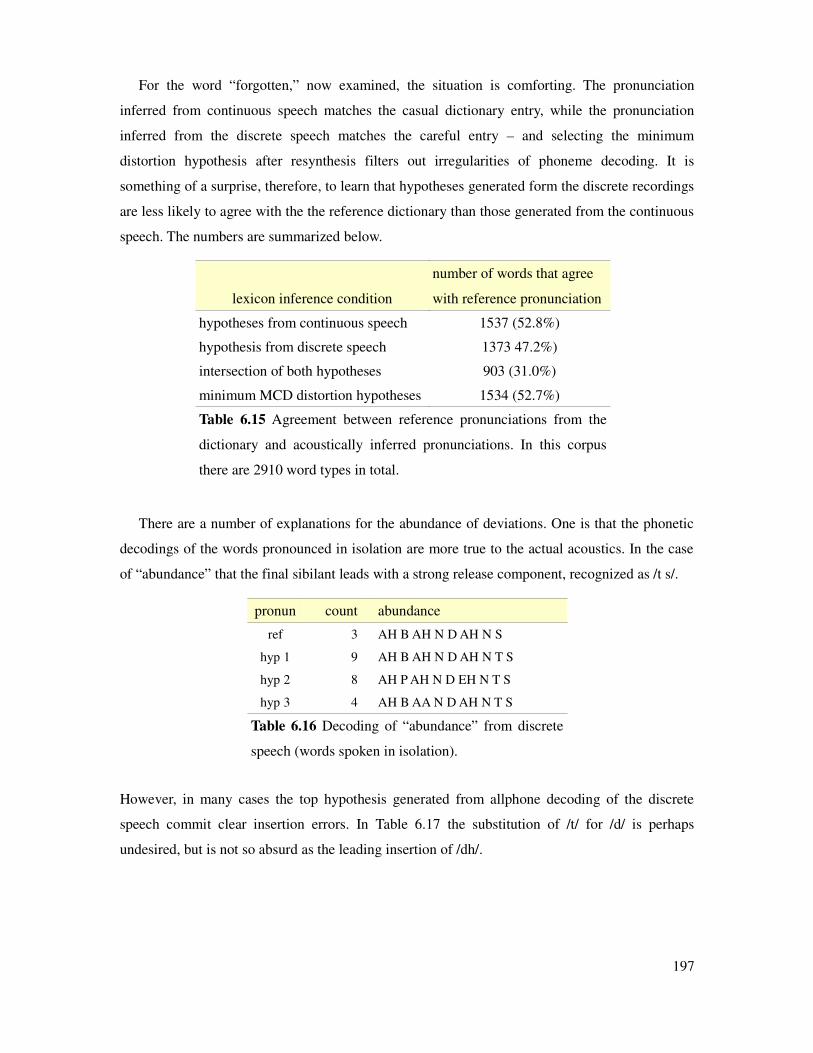
For the word “forgotten,” now examined, the situation is comforting. The pronunciation

inferred from continuous speech matches the casual dictionary entry, while the pronunciation

inferred from the discrete speech matches the careful entry – and selecting the minimum

distortion hypothesis after resynthesis filters out irregularities of phoneme decoding. It is

something of a surprise, therefore, to learn that hypotheses generated form the discrete recordings

are less likely to agree with the the reference dictionary than those generated from the continuous

speech. The numbers are summarized below.

lexicon inference condition

number of words that agree

with reference pronunciation

hypotheses from continuous speech 1537 (52.8%)

hypothesis from discrete speech 1373 47.2%)

intersection of both hypotheses 903 (31.0%)

minimum MCD distortion hypotheses 1534 (52.7%)

Table 6.15 Agreement between reference pronunciations from the

dictionary and acoustically inferred pronunciations. In this corpus

there are 2910 word types in total.

There are a number of explanations for the abundance of deviations. One is that the phonetic

decodings of the words pronounced in isolation are more true to the actual acoustics. In the case

of “abundance” that the final sibilant leads with a strong release component, recognized as /t s/.

pronun count abundance

ref 3 AH B AH N D AH N S

hyp 1 9 AH B AH N D AH N T S

hyp 2 8 AH P AH N D EH N T S

hyp 3 4 AH B AA N D AH N T S

Table 6.16 Decoding of “abundance” from discrete

speech (words spoken in isolation).

However, in many cases the top hypothesis generated from allphone decoding of the discrete

speech commit clear insertion errors. In Table 6.17 the substitution of /t/ for /d/ is perhaps

undesired, but is not so absurd as the leading insertion of /dh/.

197

pronun count absurd

ref 2 AH B S ER D

hyp 1 12 DH AE T S ER D

hyp 2 10 AE T S ER D

hyp 3 2 AH T S ER D

Table 6.17 Decoding of “absurd” from discrete speech.

What appears to be happening is that for vowel-onset words there is weak but audible speech

at the beginning that is decoded to its own phone, rather than being discarded as silence. Another

word in which this happens is the word “air.”

pronun count air

ref 2 EH R

hyp 1 14 DH EY ER

hyp 2 10 B EY ER

hyp 3 4 D EY ER

Table 6.18 Decoding of “air” from discrete speech.

The attempt by the decoder to interpret the diphthong as /ey er/ quite acceptable, but the

propensity to insert a leading stop consonant is less so. Consonant insertion is seen in some

situations word-finally, also.

pronun count also

ref 5 AO L S OW

hyp 1 14 AO L S OW L

hyp 2 5 DH AH AO L S OW L

hyp 3 4 AO L S OW N

Table 6.19 Decoding of “also” from discrete speech.

There are likely many other phonological decoding effects that we haven't presented here and

are worth describing. The intent is not to be exhaustive, but to highlight some frequent patterns

that illuminate the results of lexicon inference from acoustic evidence. What emerges clearly

from the experiments is the benefit of filtering hypotheses through minimal distortion resynthesis.

While this method is not immune to idiosyncrasies, it applies a strong constraint on acoustically-

derived pronunciations so that they are sensible linguistically, and tuned to the requirements of

text-to-speech.

198

7 Conclusions

7.1 Contributions

A non-technical user faces fundamental challenges when attempting to build speech synthesizers

for languages having very limited resources. This thesis has examined many of the challenges in

depth. Our contributions make significant progress in solving “TTS from Zero.” We recap these

contributions and then conclude with potential future work.

7.1.1 G2P Rules

In the pivotal area of grapheme-to-phoneme conversion, we have developed a G2P rule learning

system based on expanding context linear rule chains. Experiments on multiple languages with

large dictionaries demonstrate excellent prediction accuracy. The high accuracy is observed both

when the lexicon is large (over 50k words) and when it is small (under 500 words). Multiple

pronunciations can be predicted for a given word through a mechanism of multi-rule triggering,

described in section 3.1.6 . In addition, the system is capable of incremental updating of the rule

chains. This enables the software to respond quickly enough that it may be used in an interactive

setting (using computers considered current).

Our “lexlearner” software is deployed in a web-based server environment. It has been used for

bootstrapping lexicons in new languages, including the suite of non-English languages analyzed

in section 5.2.2 . The order in which words are presented to the user can negatively impact the

rate of rule learning, for it is obvious that a sequence redundant words (that possess no new G2P

phenomena) will slow down the process. Section 3.4 investigated several active learning

algorithms that consider n-gram coverage and make use of the current set of rule to exercise

control over data sampling. Experiments performed on Italian indicate some gains, but that

random sampling is an acceptable word selection strategy.

199

The complexity of a language's sound system affects how quickly the corresponding G2P rules

can achieve a certain level of accuracy on unseen words. The experiments of section 3.3 broad

spectrum from highly regular Spanish to highly irregular systems of English and Arabic. as a way

to estimate the difficulty posed by language's orthographic/phonetic relation, an entropy-based

measure of rule complexity was developed in section 3.1.5 and applied in 3.3.2 .

7.1.2 User studies

Another valuable contribution are our user studies of lexicon construction. This involved the

deployment of lexicon verification software into the real-world situation of constructing an Iraqi

Arabic dictionary of named entities. So that the native speakers are not required to have facility

with phonemic representation, our software presents a list of six candidate pronunciations with

associated synthesized wavefiles, amongst which the users selects the best candidate. This

approach is novel. Detailed measurements of task completion times recorded at the mouse-click

level are also new. This allows calculation of the overall rate of processing words, as well as the

average time spent playing the wavefiles followed by making a decision.

A particularly interesting result was the discovery of two distinct modes of operation. The first

is a fast mode of checking just two wavefiles then selecting one. The second is a slow mode that

is signified by listening to all the presented wavefiles once, then double-checking the preferred

pronunciation before making proceeding with the next word. There are a couple other minor

mode. When the decision is a difficult one, the log files reveal dozens of wavefile plays before a

decision is reached. Occasionally no pronunciation is acceptable an the human reviewer resorts to

a type-in correction. The time required under this situation can exceed two minutes per word, and

so is to be avoided whenever possible.

7.1.3 MCD Calibration

Mean mel cepstral distortion (MCD) is an objective measure of voice quality that is convenient to

apply. Because differences may readily be compared between different builds of the same voice,

we conducted extensive experiments to discover trends that may informative across speakers and

even languages. The investigation, beginning in section 5.1.2 , determined of which symbolic

and numeric training features are most predictive at the acoustic level of cepstral frames, and to

what extent the size surrounding context helps. This led to an identification of a minimal set of

ten features that predicts 95% as well as the full set. In an important discovery we found that

language-dependent features are substantially less critical than language-independent features.

200

This contribution removes the concern that sophisticated linguistic knowledge is necessary for

new voice development.

Another major contribution is the discovery of a log-linear relationship between MCD and

corpus size – that a doubling of data reduces MCD by 0.12. This relation holds over at least five

doublings in the size of English speech data. Continuing our efforts to calibrate MCD with

English, we measured the quantitative effect that having a mature lexicon provides. This was

accomplished by comparing phoneme-based versus rudimentary grapheme-based voices. The

combination of these two results provides calibration lines for evaluating new voices in other

language. In Figure 5.10 the calibration marks provides a context for estimating the quality of

eight non-English languages built from small amounts of data.

7.1.4 Iterative voice building

Once a user has succeeds in building an initial voice from limited data, they face the question of

what to do next. Iterative voice building provides a technique for interleaving the three major

tasks of recording, lexicon development, and quality assessment. By conducting a pilot

experiment we found that 20-25 minutes spent per task is a workable commitment of time, i.e.

before user fatigue sets in. Including task transition time, this translates to about an hour and a

half per iteration. What was not known prior to running this experiment was the relative

efficiency of the three tasks: in particular, a comparison of the time spent recording new speech

versus that devoted to lexical work. Also not know was the comparative improvement made to

the voice by each task. Once several voices were developed through five stage of iteration, the

relative reduction in MCD was measured after each step. From this information one can compute

change in MCD per hour of work, for both recording and lexicon development, as the voice

grows in size. This information is new. As discussed in section 5.4.6 , one can identify a

transition point: from where recording more speech is most effective (when the voice is small), to

where working on the lexicon offers more efficient gains in voice quality.

In addition to measuring MCD, we also measured voice quality through transcription of held

out test sentences, and through comparative AB listening tests. Transcription tests provide a direct

measure of voice intelligibility, and thus an indication of when it is good enough to be

deployable. What is “good enough” depends on the complexity of the domain. For the domain

investigated (cooking recipes: a constrained but open ended language domain), the user will want

to invest at least five hours of development time to achieve a successful voice.

201

7.1.5 Correlating objective to subjective quality measures

During the iterative voice building experiment, voice quality was measured using three separate

kinds of tests: objective (MCD), semi-subjective (sentence transcription), and subjective (AB

preference comparisons). The raw data from the first is a floating point number. From the second

it is a set of minimum edit distance alignments, which are distilled down to transcription word

error rate. From the third are a set of trinary decisions (when ties are allowed), which for each

pair of systems one can compute a preference percentage. Finding a relationship between these

three measures would be of great benefit. In section 5.4 we brought the technique of statistical

rating systems know as Bradley-Terry models to bear on the problem. The technique, as it is

commonly used to rate professional chess and go players, converts a set of AB comparisons

between n players into a set of scalar values, with one value assigned to each player (their rating).

Once this conversion is performance, the rating of a voice derived from AB listening tests is

readily compared to MCD values and transcription error rates.

Initial results, as plotted in Figure 5.15, indicate a linear relation – over the range examined –

between MCD and AB preference rating. Specifically, that a doubling of size of speech

corresponds to a reducing in MCD of 0.12, which corresponds to an AB preference of 66%. This

particular relation, and the method for establishing it, are a novel contribution of this thesis.

7.1.6 Lexicon inference from acoustics

After an outline of the overall approach, we developed a novel algorithm for automatic inference

of word pronunciations from acoustic evidence. The key idea has three components: 1) use of

automatic speech recognition run in phoneme decoding mode to generate pronunciation

hypotheses, 2) use of a speech synthesizer to resynthesize each hypothesis, and 3) a comparison

of the various synthesized utterances with the original wavefile to select the minimum mean

cepstral distortion pronunciation. (The ASR and TTS components may be built from the same

single-speaker data. Alternatively, an existing set of acoustic models may be adapted to the

speaker.) Section 6.4.3 documents the considerable advantage of running ASR-generated

hypotheses through the filter of TTS.

One aspect of this work is the ability to compare pronunciations automatically extracted from

isolated words (discrete speech), and from words spoken in the context of continuous speech.

This supports the discovery of post-lexical phonological rules, and the development of lexicons

with multi-tiered representation. It also allows a speech technologist to position a lexicon along

202

the spectrum of carefully dictated to casually spoken speech.

In our specific experiment, each of the 2910 words present in the Arctic vocabulary was

spoken twice in isolation. Having a set of dual recordings is useful. Two examples supports

greater confidence in word's inferred pronunciation. It also provides for an estimate of

pronunciation variability, and examples of alternations present in words that are nominally

identical. Even though the isolated word corpus follows the original Arctic recordings by several

years [100], it nevertheless provides an interesting adjunct. This data is freely available for

download from the same source [41].

7.2 Future Work

The investigations of this thesis suggest several continuing directions for further research.

In Chapter 6 we outlined a minimum distortion, analysis-by-synthesis framework for inferring

word pronunciations from acoustic evidence. The same synthesizer-oriented decision framework

(of adopting the minimum MCD choice) may potentially be used to select the best merge/split

operation during phoneset refinement. This possibility is open to investigation. Also, it is worth

pointing out that the ASR acoustic models and TTS voice models are not only separately trained,

but different in representation. The development of unified acoustic models is a topic of active

research [167] that warrants investigation.

Section 5.4 established a means of relating objective, subjective, and semi-subjective qualities

measures, and applied it to the incremental voice building experiments. These methods are worth

applying to other databases to refine the quantitative relationships discovered. It would also be

valuable to push the calibration experiments of section 5.1 beyond a single hour of speech.

Section 5.3 explored incremental voice building for English. We measured the time required

to perform component tasks, and the corresponding improvement in voice quality. A natural

extension is to apply this work to other languages. For example, in continuing voice development

of the eight small-scale non-English languages studied in section 5.2.2 . When engaged in

incremental voice building there is always the underlying question of when it is okay to stop

doing more work and deploy the synthesizer. This answer is surely language-specific, domain-

specific, and task-specific. Held out transcription tests are good for measuring intelligibility, and

one could posit, say, a 2% transcription error rate as the decision threshold. However, the true test

is to use the synthesizer in a realistic application setting, such as that of chapter 4 . One solution

is to approach from the opposite direction: to take a high-quality synthesizer and progressively

203

degrade it while measuring task-specific comprehensibility. This can be then compared to the

build-it-from-zero approach to locate a place of intersection.

The flip side of “when can I stop?” is the problem of motivating the users to continue working

until this point is reached. This is largely a matter of human-computer interaction. As a general

answer – the results of incremental builds offers perceptible improvements, and that a system that

is clearly improving encourages continuing effort. In our experiments each task had a granularity

of about 20 minutes, with a full iteration requiring an hour and a half of effort. It is possible that

the granularity of feedback can be tightened by an order of magnitude. It is also possible that our

calibration experiments can be used to offer “percent complete” information that is continuously

updated and displayed.

Finally, reducing the effort required of users is always a valuable pursuit. We found that the

time required of native speakers reviewing the lexicon remains the largest bottleneck, particularly

for languages having a complex grapheme-to-phoneme sound system. If our process of

automatically deriving pronunciations from acoustics can be made to work when bootstrapping

from small amounts of data, then the savings in human effort promises to be substantial.

204

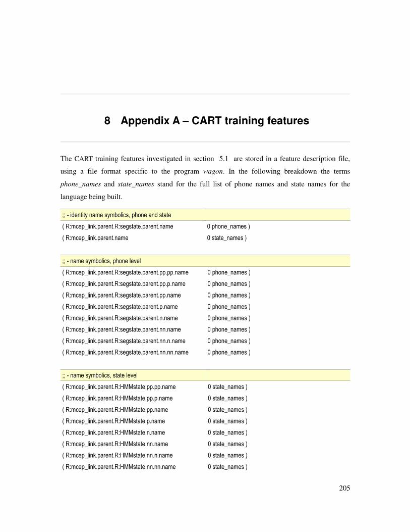
8 Appendix A – CART training features

The CART training features investigated in section 5.1 are stored in a feature description file,

using a file format specific to the program wagon. In the following breakdown the terms

phone_names and state_names stand for the full list of phone names and state names for the

language being built.

;; - identity name symbolics, phone and state

( R:mcep_link.parent.R:segstate.parent.name 0 phone_names )

( R:mcep_link.parent.name 0 state_names )

;; - name symbolics, phone level

( R:mcep_link.parent.R:segstate.parent.pp.pp.name 0 phone_names )

( R:mcep_link.parent.R:segstate.parent.pp.p.name 0 phone_names )

( R:mcep_link.parent.R:segstate.parent.pp.name 0 phone_names )

( R:mcep_link.parent.R:segstate.parent.p.name 0 phone_names )

( R:mcep_link.parent.R:segstate.parent.n.name 0 phone_names )

( R:mcep_link.parent.R:segstate.parent.nn.name 0 phone_names )

( R:mcep_link.parent.R:segstate.parent.nn.n.name 0 phone_names )

( R:mcep_link.parent.R:segstate.parent.nn.nn.name 0 phone_names )

;; - name symbolics, state level

( R:mcep_link.parent.R:HMMstate.pp.pp.name 0 state_names )

( R:mcep_link.parent.R:HMMstate.pp.p.name 0 state_names )

( R:mcep_link.parent.R:HMMstate.pp.name 0 state_names )

( R:mcep_link.parent.R:HMMstate.p.name 0 state_names )

( R:mcep_link.parent.R:HMMstate.n.name 0 state_names )

( R:mcep_link.parent.R:HMMstate.nn.name 0 state_names )

( R:mcep_link.parent.R:HMMstate.nn.n.name 0 state_names )

( R:mcep_link.parent.R:HMMstate.nn.nn.name 0 state_names )

205

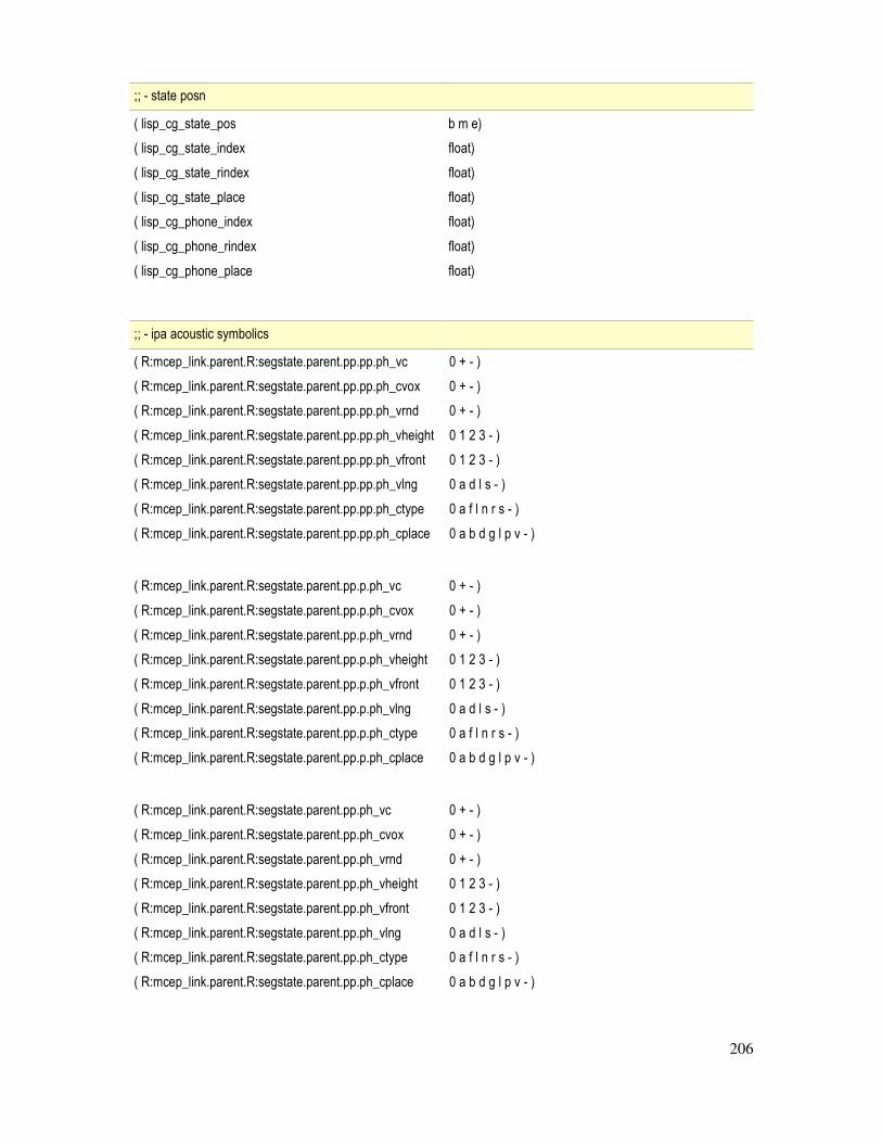
;; - state posn

( lisp_cg_state_pos b m e)

( lisp_cg_state_index float)

( lisp_cg_state_rindex float)

( lisp_cg_state_place float)

( lisp_cg_phone_index float)

( lisp_cg_phone_rindex float)

( lisp_cg_phone_place float)

;; - ipa acoustic symbolics

( R:mcep_link.parent.R:segstate.parent.pp.pp.ph_vc 0 + - )

( R:mcep_link.parent.R:segstate.parent.pp.pp.ph_cvox 0 + - )

( R:mcep_link.parent.R:segstate.parent.pp.pp.ph_vrnd 0 + - )

( R:mcep_link.parent.R:segstate.parent.pp.pp.ph_vheight 0 1 2 3 - )

( R:mcep_link.parent.R:segstate.parent.pp.pp.ph_vfront 0 1 2 3 - )

( R:mcep_link.parent.R:segstate.parent.pp.pp.ph_vlng 0 a d l s - )

( R:mcep_link.parent.R:segstate.parent.pp.pp.ph_ctype 0 a f l n r s - )

( R:mcep_link.parent.R:segstate.parent.pp.pp.ph_cplace 0 a b d g l p v - )

( R:mcep_link.parent.R:segstate.parent.pp.p.ph_vc 0 + - )

( R:mcep_link.parent.R:segstate.parent.pp.p.ph_cvox 0 + - )

( R:mcep_link.parent.R:segstate.parent.pp.p.ph_vrnd 0 + - )

( R:mcep_link.parent.R:segstate.parent.pp.p.ph_vheight 0 1 2 3 - )

( R:mcep_link.parent.R:segstate.parent.pp.p.ph_vfront 0 1 2 3 - )

( R:mcep_link.parent.R:segstate.parent.pp.p.ph_vlng 0 a d l s - )

( R:mcep_link.parent.R:segstate.parent.pp.p.ph_ctype 0 a f l n r s - )

( R:mcep_link.parent.R:segstate.parent.pp.p.ph_cplace 0 a b d g l p v - )

( R:mcep_link.parent.R:segstate.parent.pp.ph_vc 0 + - )

( R:mcep_link.parent.R:segstate.parent.pp.ph_cvox 0 + - )

( R:mcep_link.parent.R:segstate.parent.pp.ph_vrnd 0 + - )

( R:mcep_link.parent.R:segstate.parent.pp.ph_vheight 0 1 2 3 - )

( R:mcep_link.parent.R:segstate.parent.pp.ph_vfront 0 1 2 3 - )

( R:mcep_link.parent.R:segstate.parent.pp.ph_vlng 0 a d l s - )

( R:mcep_link.parent.R:segstate.parent.pp.ph_ctype 0 a f l n r s - )

( R:mcep_link.parent.R:segstate.parent.pp.ph_cplace 0 a b d g l p v - )

206

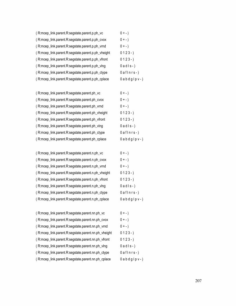
( R:mcep_link.parent.R:segstate.parent.p.ph_vc 0 + - )

( R:mcep_link.parent.R:segstate.parent.p.ph_cvox 0 + - )

( R:mcep_link.parent.R:segstate.parent.p.ph_vrnd 0 + - )

( R:mcep_link.parent.R:segstate.parent.p.ph_vheight 0 1 2 3 - )

( R:mcep_link.parent.R:segstate.parent.p.ph_vfront 0 1 2 3 - )

( R:mcep_link.parent.R:segstate.parent.p.ph_vlng 0 a d l s - )

( R:mcep_link.parent.R:segstate.parent.p.ph_ctype 0 a f l n r s - )

( R:mcep_link.parent.R:segstate.parent.p.ph_cplace 0 a b d g l p v - )

( R:mcep_link.parent.R:segstate.parent.ph_vc 0 + - )

( R:mcep_link.parent.R:segstate.parent.ph_cvox 0 + - )

( R:mcep_link.parent.R:segstate.parent.ph_vrnd 0 + - )

( R:mcep_link.parent.R:segstate.parent.ph_vheight 0 1 2 3 - )

( R:mcep_link.parent.R:segstate.parent.ph_vfront 0 1 2 3 - )

( R:mcep_link.parent.R:segstate.parent.ph_vlng 0 a d l s - )

( R:mcep_link.parent.R:segstate.parent.ph_ctype 0 a f l n r s - )

( R:mcep_link.parent.R:segstate.parent.ph_cplace 0 a b d g l p v - )

( R:mcep_link.parent.R:segstate.parent.n.ph_vc 0 + - )

( R:mcep_link.parent.R:segstate.parent.n.ph_cvox 0 + - )

( R:mcep_link.parent.R:segstate.parent.n.ph_vrnd 0 + - )

( R:mcep_link.parent.R:segstate.parent.n.ph_vheight 0 1 2 3 - )

( R:mcep_link.parent.R:segstate.parent.n.ph_vfront 0 1 2 3 - )

( R:mcep_link.parent.R:segstate.parent.n.ph_vlng 0 a d l s - )

( R:mcep_link.parent.R:segstate.parent.n.ph_ctype 0 a f l n r s - )

( R:mcep_link.parent.R:segstate.parent.n.ph_cplace 0 a b d g l p v - )

( R:mcep_link.parent.R:segstate.parent.nn.ph_vc 0 + - )

( R:mcep_link.parent.R:segstate.parent.nn.ph_cvox 0 + - )

( R:mcep_link.parent.R:segstate.parent.nn.ph_vrnd 0 + - )

( R:mcep_link.parent.R:segstate.parent.nn.ph_vheight 0 1 2 3 - )

( R:mcep_link.parent.R:segstate.parent.nn.ph_vfront 0 1 2 3 - )

( R:mcep_link.parent.R:segstate.parent.nn.ph_vlng 0 a d l s - )

( R:mcep_link.parent.R:segstate.parent.nn.ph_ctype 0 a f l n r s - )

( R:mcep_link.parent.R:segstate.parent.nn.ph_cplace 0 a b d g l p v - )

207

( R:mcep_link.parent.R:segstate.parent.nn.n.ph_vc 0 + - )

( R:mcep_link.parent.R:segstate.parent.nn.n.ph_cvox 0 + - )

( R:mcep_link.parent.R:segstate.parent.nn.n.ph_vrnd 0 + - )

( R:mcep_link.parent.R:segstate.parent.nn.n.ph_vheight 0 1 2 3 - )

( R:mcep_link.parent.R:segstate.parent.nn.n.ph_vfront 0 1 2 3 - )

( R:mcep_link.parent.R:segstate.parent.nn.n.ph_vlng 0 a d l s - )

( R:mcep_link.parent.R:segstate.parent.nn.n.ph_ctype 0 a f l n r s - )

( R:mcep_link.parent.R:segstate.parent.nn.n.ph_cplace 0 a b d g l p v - )

( R:mcep_link.parent.R:segstate.parent.nn.nn.ph_vc 0 + - )

( R:mcep_link.parent.R:segstate.parent.nn.nn.ph_cvox 0 + - )

( R:mcep_link.parent.R:segstate.parent.nn.nn.ph_vrnd 0 + - )

( R:mcep_link.parent.R:segstate.parent.nn.nn.ph_vheight 0 1 2 3 - )

( R:mcep_link.parent.R:segstate.parent.nn.nn.ph_vfront 0 1 2 3 - )

( R:mcep_link.parent.R:segstate.parent.nn.nn.ph_vlng 0 a d l s - )

( R:mcep_link.parent.R:segstate.parent.nn.nn.ph_ctype 0 a f l n r s - )

( R:mcep_link.parent.R:segstate.parent.nn.nn.ph_cplace 0 a b d g l p v - )

;; - linguistic

( R:mcep_link.parent.R:segstate.parent.R:SylStructure.parent.stress 0 1 )

( R:mcep_link.parent.R:segstate.parent.R:SylStructure.parent.accented 0 1 )

( R:mcep_link.parent.R:segstate.parent.syl_initial 0 1 )

( R:mcep_link.parent.R:segstate.parent.syl_final 0 1 )

( R:mcep_link.parent.R:segstate.parent.pos_in_syl 0 1 2 3 4 5 6 7 )

( R:mcep_link.parent.R:segstate.parent.seg_onsetcoda 0 coda onset )

( R:mcep_link.parent.R:segstate.parent.n.seg_onsetcoda 0 coda onset )

( R:mcep_link.parent.R:segstate.parent.p.seg_onsetcoda 0 coda onset )

( R:mcep_link.parent.R:segstate.parent.R:SylStructure.parent.syl_break 0 1 2 3 4 )

( R:mcep_link.parent.R:segstate.parent.R:SylStructure.parent.R:Syllable.p.syl_break 0 1 2 3 4 )

( R:mcep_link.parent.R:segstate.parent.R:SylStructure.parent.position_type 0 initial single final mid )

( R:mcep_link.parent.R:segstate.parent.R:SylStructure.parent.parent.gpos 0 aux cc content det in md

pps to wp punc )

( R:mcep_link.parent.R:segstate.parent.R:SylStructure.parent.parent.R:Word.p.gpos 0 aux cc content det in md

pps to wp punc )

( R:mcep_link.parent.R:segstate.parent.R:SylStructure.parent.parent.R:Word.n.gpos 0 aux cc content det in md

pps to wp punc )

208

9 Appendix B – Bradly-Terry Models

One of the contributions of this thesis is our attempt to relate the objective measure of MCD (mel

cepstral distortion) to the subjective measure of AB listening tests. AB tests are an example of

paired-comparison evaluation. Pair-comparison evaluation is an established way of determining

who is stronger – A or B? – when absolute strength is not open to direct measurement. Some

commonplace examples are two-team sports (hockey, soccer, baseball, basketball, etc.), two-

player sports (boxing, fencing), and two-player games (chess, checkers, go). An early use of

paired-comparison in science is found in auditory psychophysics, in which subjects were asked

when two similar tones become just noticeably different as they are separated (e.g. in loudness or

frequency).9 Paired-comparison tests contrast with tasks of absolute value estimation: for example

of listening to a tone played in isolation and ascribing to it a pitch value. In speech synthesis

evaluation, 5-point MOS (mean opinion score) tests are absolute value estimation tasks.

The recognized advantage of AB tests is that they offer more precise and reliable information

regarding relative strength. A commonly claimed disadvantage is the issue of effort. If k is the

number of systems being compared, the number of unique MOS-style measurements is simply k,

while the number of possible paired comparisons is1

2 k k−1 . This problem isn't as severe as it

might at first seem. Valid rankings of the k systems can be established from O(k) rather and O(k2)

comparisons. The technique for effort reduction is to randomly sample pairs, with the majority of

pairings between systems of nearly equal strength. This is similar in spirit to the Swiss Pairing

System employed at chess tournaments [157]; as rounds progress and players are sorted by their

performance, strong players end up playing strong players, and weak players weak, so that each

game contests opponents who are roughly balanced. As it bears on speech synthesis, a rule of

thumb is that you want 5 listening subjects to each provide 20 AB measurements per system. If

9 This approach is used to establish Weber's Law of perception.

209

there are, for instance, 10 systems being compared, the experimenter seeks10

2⋅20⋅5=500 data

points. A full all-versus-all test requires 10 choose 2⋅20⋅5=4500 comparisons. In contrast to 20

AB tests, with 500 data points one can collect 10 MOS scores per system from each user.

Estimating the relative strength of two players A and B from the results of paired-comparisons

(or of games contested) is a well studied branch of statistical inference. The most common

framework employed are so-called Bradley-Terry models [30]. These assign a scalar value called

a rating to each player on the basis of game results. Determining the set of ratings from games is

the Bradley-Terry inference problem. A general solution to this problem is provided by the

Minorization-Maximization algorithm [83]. This algorithm is a generalization of Expectation

Maximization (EM) [61]. The number of games played by each competitor does not have to be

the same, and all do not have to play each other, and the average strength of opposition does not

have to be nearly identical. This is a major advantage over assigning two points per win and 1

point per tie and summing, as is done in sports tables – such results are not reliable comparisons

unless the number of games and strength of schedule is nearly the same for all competitors. Note

that to determine the relative strength of A and B it is necessary they belong to the same network,

i.e. that a path of “A played X who played Y who played B” must exist. Ratings are purely

relative to the network in which a player participates.

The inverse of the inference problem is the prediction problem. When given two players and

their ratings, a Bradley-Terry model predicts the probability that A will beat B. When applied to

speech synthesis, the “players” A and B are two synthesizers (for the same language). The

“games” are then synthesized wavefiles that the user is asked to compare and make a preference

choice. The same utterance is synthesized by A and B. In the AB-tie variant the user may declare

A and B tied if they are very similar, rather than being forced to make a choice. This is similar to

sports such as hockey and soccer in which ties are permitted (but not baseball and basketball). It

is also similar to psychophysics experiments in which the subject makes a 3-way choice; e.g. A is

louder than B, A is quieter than B, or A and B have the same loudness. Our listening results are

based on AB-tie experiments.

The tool we use for inferring ratings from experiments is the free software program BayesElo

[15]. BayesElo is used, for example, to rate computer chess programs in the long running WBEC

Ribberkerk tournament [130]. One attractive capability of this program is its ability to provide

confidence bounds on rating estimates. A historical note: in chess, ratings are otherwise known as

“Elo points.” The name derives from the Hungarian-American physicist (and strong amateur

player) Arpad Elo, who introduced Bradley-Terry models to the United States Chess Federation in

210

1959 and established the modern rating system that is still used (with enhancements) today [168].

The Elo rating system was subsequently adopted by the International Chess Federation (FIDE) in

1969 [71]. The original Elo system is a maximum likelihood estimator, and as consequence is

unreliable when a player has won or lost all of their games. It also made simplifying assumptions

to ease calculations at a time when this was performed by pencil and paper. The BayesElo

software overcomes these weakness.

With these general remarks made, we now present some of the mathematics involved in

deriving Elo ratings from paired comparison tests. One topic not discussed is that of dynamic

rating systems in which the ratings of players incrementally updated over time as new games are

played.

9.1 Basics of rating systems

Let a paired comparison, competition, or game have a distinct number of possible game results,

which we denote ℚ. Typically ∣ℚ∣ = 2 or 3. That is, ℚ2 =win, lose or ℚ3 =win, tie, lose. Let

v∈ℝ be the value of a game result. In many sports it is traditional for v ℚ3 = (2,1,0), though to

discourage conservative play some leagues are trying v ℚ3 = (3,1,0). In Elo Rating systems a

win is normalized to one, a loss is still zero, and a tie splits the point: v ℚ3 = (1, 0.5, 0). A player

k who has competed in N games has a game record Q=qk ,1 ,qk ,2 ,qk , N . The empirical

expectation value, E , is the average of all game results.

E Q =1

N∑n=1

N

v qn (9.1)

It is convenient to collect the game results into counts of total wins, ties, and losses.

G k= gwin , g tie , g losek ,∑ g q=N . Then

E Q = E G =∑q∈Q

v g q

∑q∈Q

g q

=g

win0.5 g

tie

g wing tieglose

=g

win0.5 g

tie

N(9.2)

In eqn (9.2) the games of Gk are against any number of opponents. To predict the performance of

a player k of against a particular schedule of opponents, we first need the probability that player i

beats another player j. The suppositions of Bradley-Terry models are that a) the strength of each

player is represented by a single scalar parameter, denoted by gamma, b) the parameters are scale

invariant, and c) the equation relating player strength is monotonically increasing as a function of

211

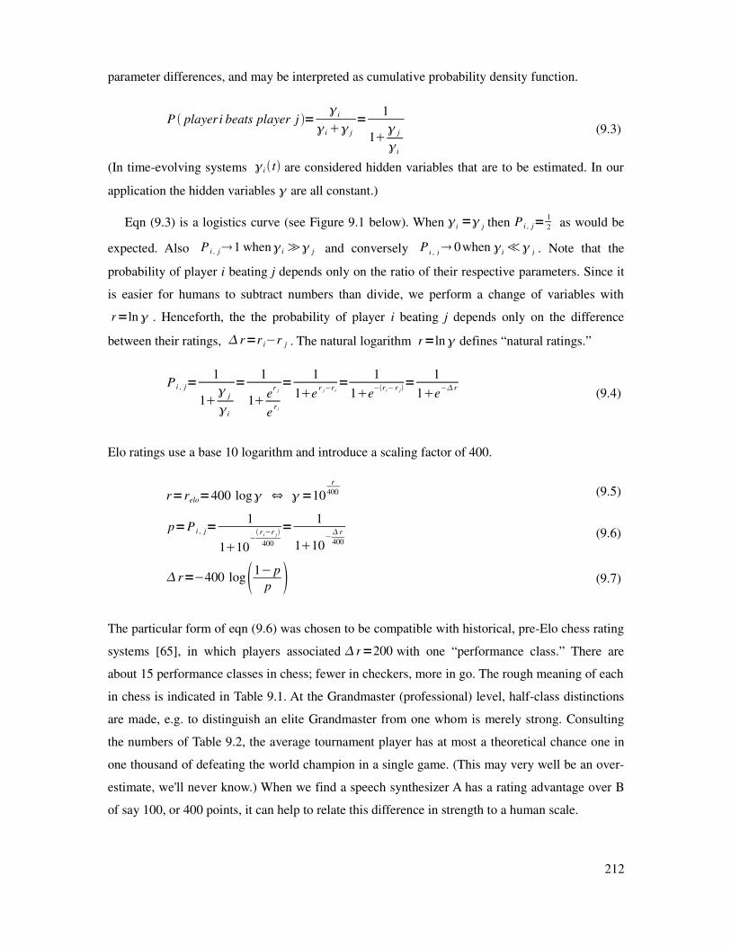
parameter differences, and may be interpreted as cumulative probability density function.

P player i beats player j =

i

i j

=1

1 j

i

(9.3)

(In time-evolving systems i t are considered hidden variables that are to be estimated. In our

application the hidden variables are all constant.)

Eqn (9.3) is a logistics curve (see Figure 9.1 below). When i=

j then P i , j=1

2 as would be

expected. Also P i , j1 wheni ≫ j and conversely Pi , j 0when

i≪

j . Note that the

probability of player i beating j depends only on the ratio of their respective parameters. Since it

is easier for humans to subtract numbers than divide, we perform a change of variables with

r=ln . Henceforth, the the probability of player i beating j depends only on the difference

between their ratings, r=r i−r j . The natural logarithm r=ln defines “natural ratings.”

P i , j=1

1

j

i

=1

1e

r j

er i

=1

1er j−r i

=1

1e−r i−r j

=1

1e− r

(9.4)

Elo ratings use a base 10 logarithm and introduce a scaling factor of 400.

r=relo=400 log ⇔ =10r

400 (9.5)

p=P i , j=1

110− r i−r j

400

=1

110− r

400(9.6)

r=−400 log1− p

p (9.7)

The particular form of eqn (9.6) was chosen to be compatible with historical, pre-Elo chess rating

systems [65], in which players associated r=200 with one “performance class.” There are

about 15 performance classes in chess; fewer in checkers, more in go. The rough meaning of each

in chess is indicated in Table 9.1. At the Grandmaster (professional) level, half-class distinctions

are made, e.g. to distinguish an elite Grandmaster from one whom is merely strong. Consulting

the numbers of Table 9.2, the average tournament player has at most a theoretical chance one in

one thousand of defeating the world champion in a single game. (This may very well be an over-

estimate, we'll never know.) When we find a speech synthesizer A has a rating advantage over B

of say 100, or 400 points, it can help to relate this difference in strength to a human scale.

212

Elo range players approx. interpretation Elo range approx. interpretation

over 2800 1 world champion strength 1800-2000 class A – top untitled player

2700-2800 32 elite grandmaster 1600-1800 class B – strong tournament player

2600-2700 143 strong grandmaster 1400-1600 class C – average tournament player

2500-2600 812 grandmaster 1200-1400 class D – strong social player

2400-2500 2864 international master 1000-1200 class E – casual social player

2300-2400 5333 national master 800-1000 class F – novice player

2200-2300 12791 master 600-800 class G – beginner 2

2100-2200 19202 candidate master 400-600 class H – beginner 1

2000-2100 21382 expert 200-400 class I – early beginner

0-200 class J – minimum rating class

Table 9.1 Elo classes in chess. Player count is taken from the official October 2008 FIDE rating

list. Interpretations are an amalgamation of FIDE and USCF descriptions. Note that Master,

International Master, and Grandmaster are official FIDE titles achieved from tournament play,

and are not awarded solely based on ratings.

∆r P(win) P(lose) ∆r P(win) P(lose)

0 .5000 .5000 600 .9693 .0307

50 .5715 .4285 700 .9825 .0175

100 .6401 .3599 800 .9901 .0099

200 .7597 .2403 900 .9944 .0056

300 .8490 .1510 1000 .9968 .0032

400 .9091 .0909 1100 .9982 .0018

500 .9468 .0532 1200 .9990 .0010

Table 9.2 Probability of winning as a function of rating difference.

While winning probability depends only on rating difference, probabilities do not multiply across

differences. That is, if r1< r2 < r3 then P r3−r 1≠P r 3−r 2P r 2−r1 . For example if r1=0,

r2=400, and r3=800, then P r3−r 1=1

101≠ 1

121 while P r3−r2 =P r2−r1 =1

11 . The discrepancy is

due to the linear 2⋅10−x term in the following denominator.

P2 r=

1

110− x

1

110−x

=1

12⋅10−x10

−2x , x= r

400(9.8)

213

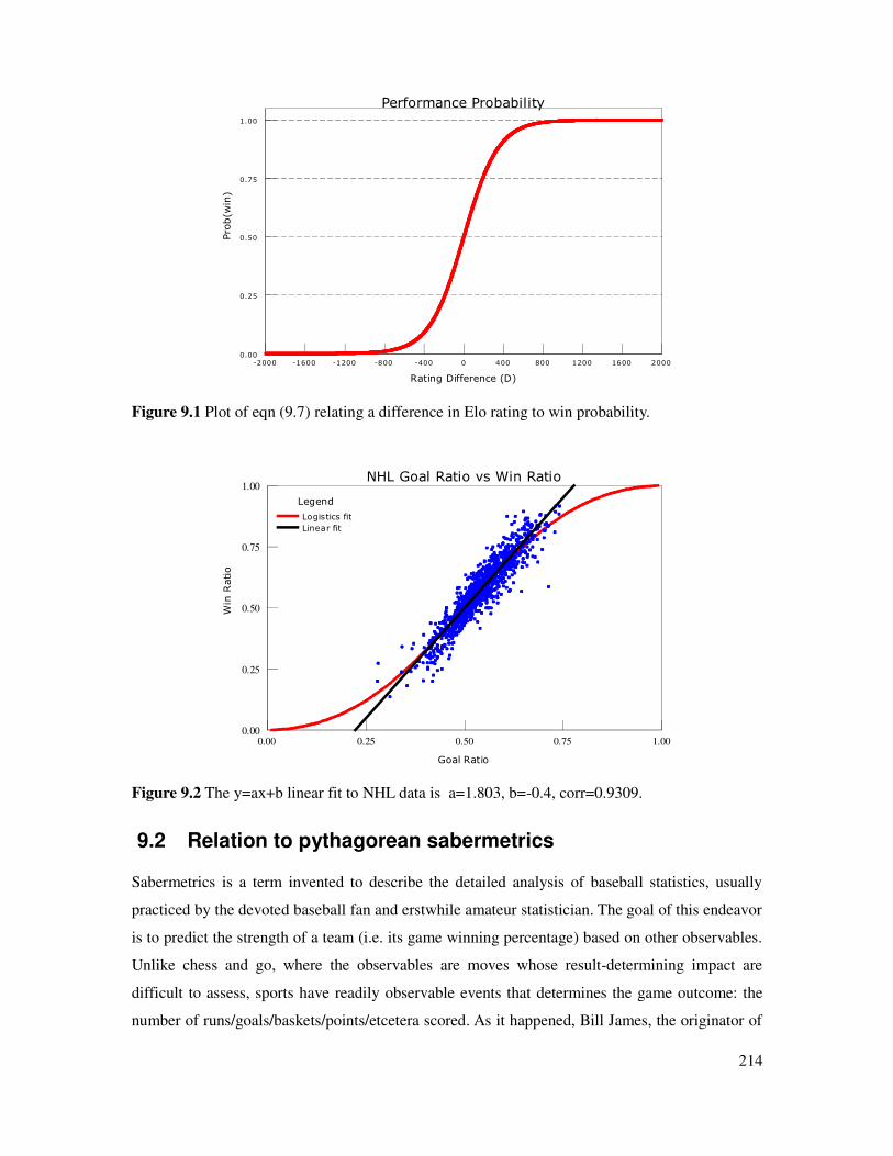
Figure 9.1 Plot of eqn (9.7) relating a difference in Elo rating to win probability.

Figure 9.2 The y=ax+b linear fit to NHL data is a=1.803, b=-0.4, corr=0.9309.

9.2 Relation to pythagorean sabermetrics

Sabermetrics is a term invented to describe the detailed analysis of baseball statistics, usually

practiced by the devoted baseball fan and erstwhile amateur statistician. The goal of this endeavor

is to predict the strength of a team (i.e. its game winning percentage) based on other observables.

Unlike chess and go, where the observables are moves whose result-determining impact are

difficult to assess, sports have readily observable events that determines the game outcome: the

number of runs/goals/baskets/points/etcetera scored. As it happened, Bill James, the originator of

214

Rating Difference (D)

-2000 -1600 -1200 -800 -400 0 400 800 1200 1600 2000

Prob(w

in)

0.00

0.25

0.50

0.75

1.00

Performance Probability

Goal Ratio

0.00 0.25 0.50 0.75 1.00

Win Ratio

0.00

0.25

0.50

0.75

1.00NHL Goal Ratio vs Win Ratio

Legend

Logistics fit

Linear fit

Sabermetrics, accidentally discovered that the Pythagorean theorem of elementary trigonometry

is a good predictor of baseball outcomes [87], and this has deep ties to the Elo rating system. In

2006 Miller proved that if the run-generating random process adheres a Weibull distribution then

the “Pythagorean formula” of James is equivalent to a Bradley-Terry model [119]. The proof is

not repeated here, but the connection between run ratios, winning expectation, and Elo ratings is

illuminating.

If c is the hypotenuse of a right angled triangle, with sides a and b, then in Euclidean geometry

c2=a

2b2 . With c=acos the identity can be written in the Bradley-Terry form of eqn (9.3).

cos2=

a2

c2=

a2

a2b

2=

1

1 b

a 2=

1

1b

2

a2

=1

1 b

a

,

b=b

2

a=a

2(9.9)

This becomes less abstract when meaning is associated with the Pythagorean variables: a is

assigned to the average number of runs team A scores, b is the average number of runs of the

opponent B. A generalization of eqn (9.9) is claimed to provide the probability that A beats B,

P A beats B=a

ab

=1

1b

a

(9.10)

where the exponent is a free parameter fitted to game data. The best exponent depends on the

type of sport played. In particular, on the average number points scored per game. In Major

League baseball the empirical exponent is 1.81 (it predicts better than the strictly Pythagorean 2)

while in higher-scoring basketball it lies in the range of 8-9 [169]. When fitted to the entire

history of NHL hockey games, the value is similar to baseball: 1.80, plotted in Figure 9.2 above.

The exponent is estimated by performing a least-squares linear fit to the data, after a performing

change of variables. Let x be the ratio of average runs scored by team A.

x=a

ab, 1−x=

b

ab, x∈[0,1] (9.11)

Then the expected win ratio is expressed in terms of run ratios by substituting (9.11) into (9.10).

P=a

ab

1

ab

1

ab

= a

ab

a

ab

b

ab =

x

x1−x

=1

1 1

x−1

(9.12)

215

When =1 eqn (9.12) is a straight line from (0,0) to (1,1). The first derivative equals when

evaluated at x= 1

2 , found by applying the Quotient Rule of elementary calculus.

dP

dx=

x2 1

x−1

−1

[1 1

x−1

]2

,dP x=0.5

dx= (9.13)

Elo ratings can be related to the empirically measured and to scoring productivity.

rA=400 log a , a=average number of runs/goals scored by team A (9.14)

r=400 loga

b=400 log a−log b (9.15)

Eqn (9.15) suggests a hidden relation between scored-games common in sports and with strategic

board games such as chess and go. In these games each move “scores” minor advantages (or

disadvantages), until the total accumulation reaches a decisive victory. Or, until play fails to reach

a decisive position, in which case the game is drawn. Something similar can be claimed for

subjective listening tests used in speech synthesis, except that all the little “scores” are demerit

points. When listening to a wavefile it seems, from reflection, that subjects make note of defects

in naturalness and try to assess the severity. And when comparing two wavefiles A and B, the sum

total of defects of one are weighed against the other to reach a preference decision, according to

some complicated mental formula that cannot really be fathomed.

Thus a certain perspective may be taken: a game between contestants consists of a sequence of

plays in which each side produces (or counters) points of varying strength, with the final sums

compared and adjudicated to determine a game result. Because the Central Limit theorem

establishes that the sum of any i.i.d. process tends in the limit to a Gaussian distribution, one may

take this as a fair approximation and treat contestants as Gaussian random variables. Thus, the

mean of the random variable represents absolute strength. In sports the absolute scale is directly

measured though points scored. In psychophysics experiments subjects may be asked to estimate

absolute positioning. Insofar as TTS listening tests are psychophysics experiments, MOS scale

evaluations are estimates on an absolute scale. In games such as chess, absolute strength is

difficult to determine, and so ratings rely solely on the results of AB comparisons. But the

perspective that the underlying process consists of Gaussian random variables was the theoretical

foundation upon which Arpad Elo developed his rating system. That is to say, he didn't begin with

Bradley-Terry models, but started elsewhere and ended up there as an approximation.

216

9.3 Relation to Gaussian random processes

It's a fact of competition that sometime a player or team has a good night and at other times a

poor night. One day a team's goalie has sluggish reflexes whereas the night before they were

“sharp as a cat's.” Or the star defender suffered a pulled muscle three games back and is still

feeling restricted. Whatever the various causes, the overall strength of a team varies from night to

night – it is, in mathematical terminology, a random variable. The same is true of chess strength

exhibited at the board. Noting the Central Limit Theorem, Arpad Elo put forth the assumption

that each player can be represented by a Gaussian random variable of differing means, but of

identical variance. The assumption of equal variance is an obvious approximation. A low variance

player exhibits consistent strength game after game, whereas with a high variance player you

never know whether to expect brilliancies or blunders at the table – and there are certainly some

players of this type. Nevertheless, it is a useful simplifying assumption, since it allows the

expected outcome of a match can be predicted solely form rating differences.

Let X and Y be normal random variables of identical variance 2 .

X=X x ~N 1 ,=1

2 e−x− 1

2

22

, Y =Y y ~N 2 , (9.16)

The output of each variable is some abstract measure of strength. The idea is that when each

player sits down to compete, they effectively draw a strength value from their respective

distributions. One value is subtracted from the other, z=x− y . If the difference is positive and

large the first player wins, if it is negative and large the second player wins, and within some

band of zero the game is drawn. Subtracting one random variable from another is the same as

adding its negation.

Z=X −Y =X −Y (9.17)

The range of event Zz=X Y z in the x-y plane lies to the left of the line z=x y .

Integrating this section provides the cumulative distribution function of Z.

F Z z =P X Y z=∫−∞

∞

[∫−∞

z−x

f XY x , y dy]dx (9.18)

f Z z=d

dzF Z z =∫

−∞

∞

[ d

dz∫−∞

z−x

f XY x , y dy]dx=∫−∞

∞

[ f XY x , z−x ]dx (9.19)

217

If X and Y are independent variables the function is separable.

f Z z=∫−∞

∞

f X x f Y z−x dx=∫−∞

∞

f Y y f X z− y dy , convolution (9.20)

Eqn (9.20) is immediately recognized as convolution. This allows us to proceed. By the time-shift

property of convolution, if x t ∗y t =z t then x t− 1∗y t− 2=z t− 1 2 . From

this it follows that the sum of two random variables with means X= 1 ans Y = 2 will result in a

new random variable with means added Z= 1 2 . The variance of the new distribution is

broadened compared to the component functions by Z

2= 12 2

2 , which we now show.

Recall a fundamental theorem of Fourier theory – that convolution in the time domain

corresponds to multiplication in the frequency domain f t ∗g t ⇔F G . Also, it is

fortuitous that the Fourier transform of a Gaussian is also a Gaussian.

f x =e−

x2

2 2

=2 e− 2 2

2 (9.21)

N =0, =e− 2 2

2 (9.22)

Substituting normal functions into the convolution expression.

∫−∞

∞

f Y y f X z− y dy = fX∗ f

Y (9.23)

=N 0, 1∗N 0,2 (9.24)

⇔e− 1

2 2

2e−2

2 2

2 (9.25)

=e− 1

222 2

2 (9.26)

=e−1

222

2

2

2 (9.27)

⇔e

−x

2

2 1

22

22 (9.28)

=e−

x2

2 2

, = 1

2 2

2 (9.29)

=N 0, 1

2 2

2 (9.30)

=N 0,2 , =1=

2 (9.31)

When the random variables have non-zero means, fXx =N 1 , 1 , f

Yx =N 2 , 2 we

apply the time-shift property of convolution.

218

fZ z =N 1 2 , 1

2 2

2 (9.32)

=N 1 2 ,2 , = 1= 2 (9.33)

Not forgetting that our objective is to subtract, not add, random variables, we negate y so that

Z=X −Y and f Y y f Y −y =N −2 , 2 .

fZ z =N 1 , 2∗N − 2 , 2 (9.34)

=N 1− 2 , 1

2 2

2 (9.35)

=N 1− 2 ,2 , = 1= 2(9.36)

Recall from Table 9.1 that one rating class is 200 Elo points. This is formalized by setting

=200 . Then in a game between two players fZz =N 1− 2 , 200 2 on this conventional

rating scale. The comparison is illustrated below with both players centered about R=0.

Figure 9.3 The pdf of a game between two Gaussian players is the convolution of the individual

player's density functions. With equal variances assumed, the distribution broadens by 2 .

Let r=r X−rY= 1− 2 then the probability mass above zero is the winning percentage.

Recall that the integration of a Gaussian function is not an analytic function, but is important

enough to be given permanent standing, a name z , and related to the error function erf.

z =∫−∞

z

N 0,1=1

2∫−∞

z

e−

t2

2 dt=1

2

1

2erf z

2 (9.37)

−z=1− z (9.38)

219

Rating (R)

-2000 -1500 -1000 -500 0 500 1000 1500 2000

Prob(R

)

0.0000

0.0005

0.0010

0.0015

0.0020

Gaussian Player Model

N(0,σ=200)

N(0,σ=282.2)

Legend

Player

Game

Then in a game with two results, ℚ2 =win, lose,

P lose=P X losses to Y=Z z0=∫−∞

0

N 1− 2 , 2002 (9.39)

P win=P X beats to Y=Z z0=∫0

∞

N 1− 2 ,200 2=1−P lose (9.40)

In games with three results, ℚ3 =win, tie, lose, one defines a drawing threshold T .

P lose=Z z−T=∫

−∞

−T

N 1− 2 ,200 2 (9.41)

P tie=Z −T zT =∫−T

T

N 1− 2 ,2002 =1−P win−P lose (9.42)

P win=Z zT=∫

T

∞

N 1− 2 ,200 2 (9.43)

P lose= T − 1− 2

2002 = 1

2

1

2erf

T

400 by eqn (9.37) (9.44)

The value of the drawing threshold depends on the game being contested. It is zero in games that

prohibit ties, small in high scoring games that permit ties, and large in low scoring games (such as

soccer). Figure 9.4 illustrates with T =150 and r=200 .

Figure 9.4 In a game event, players X and Y with r=200 sample once from their distributions

to produce a “strength” number. The two numbers are subtracted to decide a win/tie/loss result.

220

Rating Diff (R)

-800 -400 0 400 800 1200

Prob(R

)

0.0000

0.0005

0.0010

0.0015Result Adjudication of Gaussian Players

wintielose

Correspondingly, the cumulative density function of the Bradley-Terry model can be extended to

incorporate tied results. This is done by introducing a constant bias T in the exponent of eqn

(9.6). This has the effect decreasing the probabilities of a win or loss, with the balance going to

P(tie). In Table 9.3 a comparison is made between the two probability distributions in the case

where T =100 .

P lose=1

110

−r y−rxT

400(9.45)

P tie=1−P win−P lose (9.46)

P win=1

110

− rx−r yT

400(9.47)

P win~1

110−x P win~ x

∆r P(win) P(tie) P(lose) P(win) P(tie) P(lose)

0 .3599 .2801 .3599 .3618 .2763 .3180

100 .5000 .2598 .2403 .5000 .2602 .2398

200 .6401 .2090 .1510 .6382 .2174 .1444

300 .7598 .1493 .0909 .7602 .1611 .0786

400 .8490 .0977 .0532 .8556 .1059 .0385

500 .9091 .0603 .0307 .9214 .0167 .0169

600 .9468 .0358 .0175 .9615 .0319 .0067

700 .9694 .0208 .0099 .9831 .0146 .0023

800 .9825 .0119 .0056 .9933 .0069 .0007

Table 9.3 Example probabilities of win/tie/lose at a given ∆r, compared for T =100 . The left

side has values of the logistics model, i.e. eqns (9.45)-(9.47). The right side has value of the

Gaussian model, eqns (9.41)-(9.43).

In general, the Gaussian model assigns a slightly higher winning probabilities than does the

logistics model. This is because a Gaussian function is slightly more centrally concentrated than

the first derivative of eqn (9.6). For simplicity, adopt the natural base and let x= r /400 .

d

dxP x =

d

dx

1

1e−x

=−−e

−x

[1e−x ]

2=e−x

12e−xe

−2x=1

e−x2e

x (9.48)

221

The slight differences are illustrated in the following two plots. The discrepancy of P(r) reaches a

maximum of 1.5% around ±500 Elo points.

Figure 9.5 Cumulative density functions of logistics and Gaussian models.

Figure 9.6 Difference between curves of Figure 9.5, i.e. PG r −P Lr .

Thus if the underlying process truly is Gaussian, as Elo supposed it was for Chess players, one

can use the easier-to-manage Bradley-Terry models and be assured that the approximation error

lies with a known small bound.

222

Rating Difference (R)

-2000 -1500 -1000 -500 0 500 1000 1500 2000

Prob(R

)

0.00

0.25

0.50

0.75

1.00

Comparison of two cdf models

Legend

Logisitcs model

Gaussian model

Rating Difference (R)

-2000 -1500 -1000 -500 0 500 1000 1500 2000

∆ Prob(R

)

-0.015

-0.010

-0.005

0.000

0.005

0.010

0.015Difference in two cdf models

9.4 Direct maximum likelihood estimate

If an unrated player faces off against players with established ratings, the rating of the new player

is estimated from the average of individual performances. As an example, imagine that a

competitor play four games each against four opponents with ratings of 2000, 2100, 2200, 2300.

win tie lose ratio Ropp ∆R estimate Rest

3 0 1 .750 2000 +190.9 2190.9

2 1 1 .625 2100 +88.7 2188.7

2 0 2 .500 2200 0 2200.0

1 1 2 .375 2300 -88.7 2211.3

average 2197.7

Table 9.4 Example of rating estimate against opponents of know rating.

r=−400 log1− p / p is used to convert winning ratio to Rest.

This situation applies to speech synthesis when one has several thoroughly tested synthesizers on

hand, and one want to quickly compare these to a new version. If one assumes that the process is

Gaussian (refer to the previous section for a discussion of this), then it can be easily shown that

the average rating is the maximum likelihood estimate. One can also prove the important result

that the confidence bounds on the estimate decreases proportional to the square root of the

number of measurements.

Let X= x1 , x2 , xn be a sequence of rating estimates of an i.i.d. Gaussian player with

winning probability p x ; = p x ; , =N , .

p X ; =∏k=1

n

p x k ,=∏k=1

n1

2e− x k− 2

22

=2 2−

n

2 ∏k=1

n

e− xk− 2

22

(9.49)

Define L X ; =ln p X ; so that probabilities are cast into likelihoods.

ln p X ; =ln [2 2−

n

2 ∏k=1

n

e− xk− 2

22 ] (9.50)

=−n

2ln 2 2 ln[∏

k=1

n

e− xk− 2

22 ] (9.51)

=−n

2ln 2

2 − 1

22∑

k=1

n

xk− 2

(9.52)

223

For Gaussian processes the likelihood function is quadratic in x. Taking the derivative with

respect to the the parameter and setting equal to zero provides the maximum likelihood

estimate .

∂∂ ln p x ; =

1

2∑

k=1

n

x k− =0 (9.53)

⇒∑k=1

n

xk− =0 (9.54)

=1

n∑k=1

n

xk=x (9.55)

Figure 9.7 Two estimates of rating likelihood. The lower curve is derived from all four data

points of Table 9.4 while the upper curve is from only the contest against the R=2200 opponent.

In Figure 9.7 the width of the curves at a constant depth provides a confidence measure of the

estimate . A ∣l∣=4 vertical line is indicated. This corresponds to r=200 Elo points for

the lower curve, and r=400 points for the upper. The lower curve is derived from four times

the number data points as the upper, and thus width is halved. This can be shown by letting

r= 1− and a=−n ln 2 .

l =[a−1

22∑

k=1

n

xk− 2]−[a− 1

22∑

k=1

n

xk−1 2] (9.56)

224

Estimated Rating (R)

1800 1900 2000 2100 2200 2300 2400 2500 2600

Likelihood of

µ=R

-8

-6

-4

-2

0

Model Likelihood

∆l

∆r

1 data point

4 data points

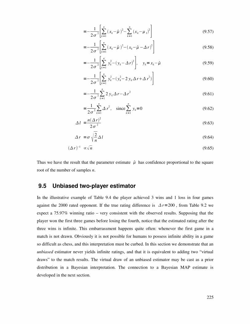
=−1

22 [∑

k=1

n

xk− 2−∑

k=1

n

x k− 12] (9.57)

=−1

22 [∑

k=1

n

xk− 2− xk− − r

2] (9.58)

=−1

22 [∑

k=1

n

yk

2− yk− r

2] , yk= xk− (9.59)

=−1

22 [∑

k=1

n

yk

2− yk

2−2 yk r r

2] (9.60)

=−1

22∑

k=1

n

2 y k r− r2

(9.61)

=1

22 ∑

k=1

n

r2, since∑

k=1

n

yk=0 (9.62)

l =n r2

2 2(9.63)

r = 2

n l (9.64)

r −1 ∝ n (9.65)

Thus we have the result that the parameter estimate has confidence proportional to the square

root of the number of samples n.

9.5 Unbiased two-player estimator

In the illustrative example of Table 9.4 the player achieved 3 wins and 1 loss in four games

against the 2000 rated opponent. If the true rating difference is r=200 , from Table 9.2 we

expect a 75.97% winning ratio – very consistent with the observed results. Supposing that the

player won the first three games before losing the fourth, notice that the estimated rating after the

three wins is infinite. This embarrassment happens quite often: whenever the first game in a

match is not drawn. Obviously it is not possible for humans to possess infinite ability in a game

so difficult as chess, and this interpretation must be curbed. In this section we demonstrate that an

unbiased estimator never yields infinite ratings, and that it is equivalent to adding two “virtual

draws” to the match results. The virtual draw of an unbiased estimator may be cast as a prior

distribution in a Bayesian interpretation. The connection to a Bayesian MAP estimate is

developed in the next section.

225

Figure 9.8 Five density functions of P p∣D = pk 1− p n−k with (k,n) = (3,3), (3,4), (6,8),

(12,16), and (24,32). D is the game results data.

Assume we have the data sequence D=q1 , q2 , q3 , q4=win ,win , win ,loss and that a game has

two results, ℚ2 =win, loss. After the first three wins are observed, the probability that the

player has a win ratio of p is shown in Figure 9.8 – as the rightmost curve having the maximal

value at p=1. Once the fourth game is included the probability density becomes the lowermost

curved centered about p=0.75. The curves immediately above show the result of collecting more

data (8, 16, 32 games) while keeping the winning ratio the same. As expected, the maximum

likelihood point is k /n . This is found in the usual way, by locating where the first derivative is

zero (and second derivate negative).

P D∣p = pk 1− p n−k (9.66)

log P D∣p =k log pn−k log 1− p (9.67)

d

dplog P D∣p =

k

p−n−k 1− p

, p∈0,1 (9.68)

k

p=

n−k

1− p, after setting

d

dplog P=0 (9.69)

1− p

p=

n−k

k(9.70)

1

p−1 =

n

k−1 (9.71)

pML =k

n(9.72)

226

p

0.00 0.25 0.50 0.75 1.00

Prob (p|D

)

0.00

0.01

0.02

0.03

0.04

0.05

0.06Probability of pararmeter p given data

Legend

n=32

n=16

n=8

n=4,k=3

n=3,k=3

And confirming the second condition.

d2

dplog P D∣p =−

k

p2−

n−k

1− p2(9.73)

=−kn

2

k2−n−k

n2

n−k 2 (9.74)

=−n

2

k−

n2

n−k=−n

2 n−k −n2k

k n−k =

−n3

k n−k 0 (9.75)

However, this maximum likelihood estimate pML is biased away from the midpoint p= 1

2 . This

is most easily seen for the (k,n) = (3,3) curve of Figure 9.8. While p = 1 is most likely, all the

other points except p = 0 are also possible, to a lesser degree. This means that on average, an

estimate closer to the center will be more accurate. The formula for pME an unbiased – or

minimum error – estimator involves computing the normalized first moment.

pME

=E p =∫0

1

p P D∣pdp

∫0

1

P D∣pdp

, p∈[0,1 ] (9.76)

The denominator integral normalizes the ratio in case the area under the curve is not 1. The

multiplier p in the numerator integral computes the center of mass of P p∣D . A fully Bayesian

calculation permits the introduction of any prior P p on the domain.

pMAP

=E p =∫0

1

p P p P D∣p dp

∫0

1

P D∣pdp

, p∈[0,1] (9.77)

Thus the formula for an unbiased estimator is equivalent to applying a uniform prior P p=1 . A

uniform prior is not terribly realistic (two evenly matched players is much more likely than one

being vastly stronger than the other), but we will find that eqn (9.76) leads to E p= pMAP=k1

n2 .

The integrals are solved by invoking properties of the Beta function B x , y .

B x , y =∫0

1

tx−1

1−ty−1

dt= x y x y

(9.78)

227

Where the gamma function is the generalization of factorial to the continuous domain.

x =∫0

∞

tx−1

e−t

dt , x∈ℝ definition (9.79)

x1 =x x recursion relation (9.80)

n =n−1! , 0 =1, n∈ℕ relation to factorial (9.81)

Substituting (9.66) into (9.77).

E p; k , n =∫0

1

p P p P D∣p dp

∫0

1

P D∣pdp

=∫0

1

pk1

1− pn−k

dp

∫0

1

pk 1− pn−k

dp

(9.82)

Perform the following change of variables to replace the integrals with gamma functions.

x−1=k1 x=k2

y−1=n−k y=n−k1for numerator (9.83)

x−1=k x=k1

y−1=n−k y=n−k1for denominator (9.84)

Then reduce to the final form.

∫0

1

pk1

1− pn− k

dp=Bk2, n−k1= k2 n−k1

n3(9.85)

∫0

1

pk1− p

n−kdp=B k1,n−k1=

k1 n−k1 n2

(9.86)

E p; k , n= k2 n3

n2 k1

=k1 n2

k1 n2

n2 k1

=k1n2

×1 (9.87)

pME=k1

n2(9.88)

In other words, to get the minimum error, pretend that the players have previously contested two

games, and each won one of them (or that both were drawn). In the BayesElo program one can

add a specified number of “virtual draws” to a tournament.

The minimum error and maximum likelihood estimates are equal at p= 1

2 and the difference

is linear in k.

228

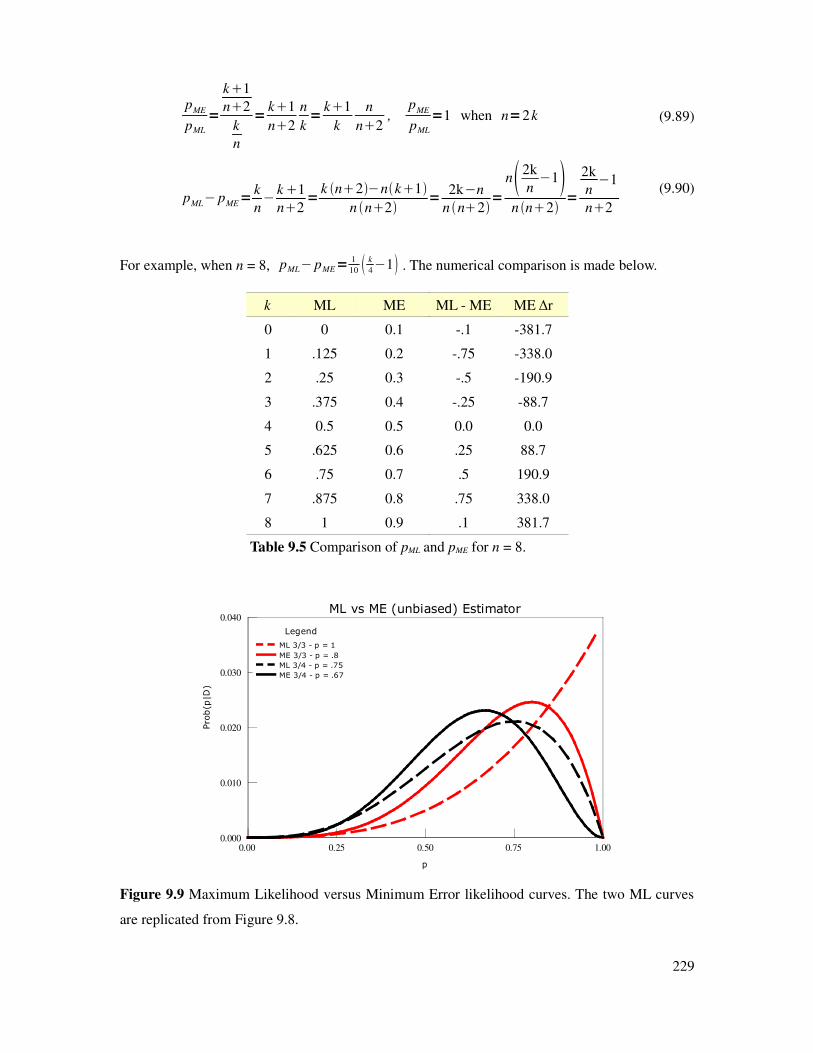
pME

pML

=

k1

n2

k

n

=k1

n2

n

k=

k1

k

n

n2,

pME

pML

=1 when n=2k (9.89)

pML− p

ME=

k

n−

k1

n2=

k n2−nk1n n2

=2k−n

n n2=

n 2k

n−1

n n2=

2k

n−1

n2

(9.90)

For example, when n = 8, pML− pME=1

10 k

4−1 . The numerical comparison is made below.

k ML ME ML - ME ME ∆r

0 0 0.1 -.1 -381.7

1 .125 0.2 -.75 -338.0

2 .25 0.3 -.5 -190.9

3 .375 0.4 -.25 -88.7

4 0.5 0.5 0.0 0.0

5 .625 0.6 .25 88.7

6 .75 0.7 .5 190.9

7 .875 0.8 .75 338.0

8 1 0.9 .1 381.7

Table 9.5 Comparison of pML and pME for n = 8.

Figure 9.9 Maximum Likelihood versus Minimum Error likelihood curves. The two ML curves

are replicated from Figure 9.8.

229

p

0.00 0.25 0.50 0.75 1.00

Prob(p|D

)

0.000

0.010

0.020

0.030

0.040ML vs ME (unbiased) Estimator

Legend

ML 3/3 - p = 1

ME 3/3 - p = .8

ML 3/4 - p = .75

ME 3/4 - p = .67

9.6 Bayesian prior of unbiased estimator

Having derived that pME=k1

n2 , let k '=k1and n '=n2 . We can separate out a Bayesian prior

of one virtual win and one virtual loss.

PME

p∣D = pk ' 1− p

n'−k '(9.91)

= pk1 1− p

n2− k1(9.92)

= pk1 1− p

n−k1(9.93)

= p 1− p pk 1− p

n−k(9.94)

= p 1− p PML

p∣D (9.95)

PMAP

p∣D =Pprior

p PML p∣D , P

prior= p 1− p (9.96)

When no actual games are played (i.e. before a match begins), the beginning probability of each

player is formally pi=1

2 and their rating difference is zero. Therefore it takes the evidence of

data to demonstrate a difference in relative strength. In general, any number of virtual win/loss

pairs can be used to define a prior with centralizing tendency. In eqn (9.97) the effect of

increasing m is to require more games to “believe” the maximum likelihood estimate.

Pprior

m p= pm1− p m (9.97)

In Figure 9.10 the MAP estimate is identical to the ME unbiased estimate of Figure 9.9.

Figure 9.10 Interpretation of the ME (unbiased) estimator as a MAP estimation – i.e. a Bayesian

prior multiplied by the ML estimate.

230

p

0.00 0.25 0.50 0.75 1.00

Prob(p)

0.00

0.01

0.02

0.03

0.04Unbiased MAP Estimator

Legend

ML 3/3 - p = 1

MAP 3/3 - p = .8

Prior 1/1 - p = .5

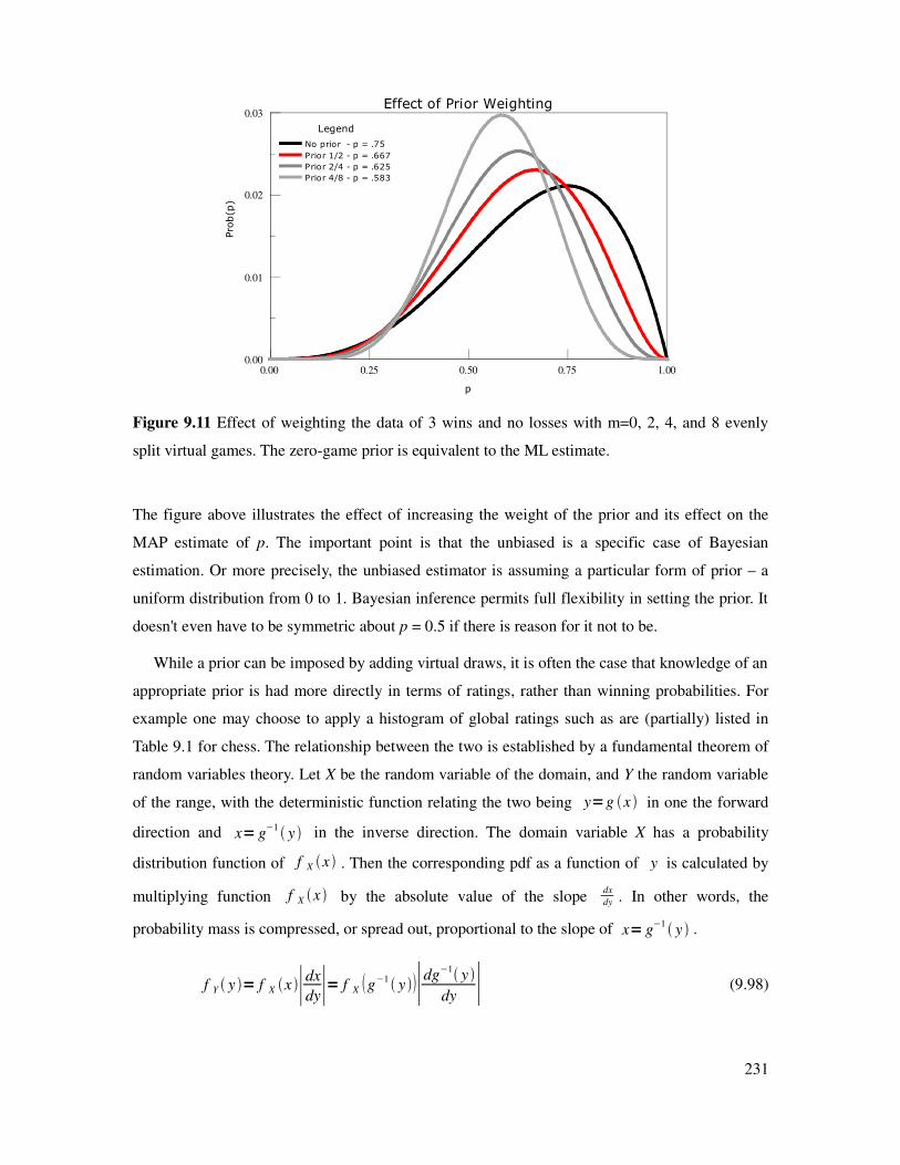
Figure 9.11 Effect of weighting the data of 3 wins and no losses with m=0, 2, 4, and 8 evenly

split virtual games. The zero-game prior is equivalent to the ML estimate.

The figure above illustrates the effect of increasing the weight of the prior and its effect on the

MAP estimate of p. The important point is that the unbiased is a specific case of Bayesian

estimation. Or more precisely, the unbiased estimator is assuming a particular form of prior – a

uniform distribution from 0 to 1. Bayesian inference permits full flexibility in setting the prior. It

doesn't even have to be symmetric about p = 0.5 if there is reason for it not to be.

While a prior can be imposed by adding virtual draws, it is often the case that knowledge of an

appropriate prior is had more directly in terms of ratings, rather than winning probabilities. For

example one may choose to apply a histogram of global ratings such as are (partially) listed in

Table 9.1 for chess. The relationship between the two is established by a fundamental theorem of

random variables theory. Let X be the random variable of the domain, and Y the random variable

of the range, with the deterministic function relating the two being y=g x in one the forward

direction and x= g−1 y in the inverse direction. The domain variable X has a probability

distribution function of f X x . Then the corresponding pdf as a function of y is calculated by

multiplying function f X x by the absolute value of the slope dx

dy . In other words, the

probability mass is compressed, or spread out, proportional to the slope of x= g−1 y .

f Y y = f X x ∣dx

dy∣= f X g−1 y ∣dg−1 y dy ∣ (9.98)

231

p

0.00 0.25 0.50 0.75 1.00

Prob(p)

0.00

0.01

0.02

0.03Effect of Prior Weighting

Legend

No prior - p = .75

Prior 1/2 - p = .667

Prior 2/4 - p = .625

Prior 4/8 - p = .583

Replacing these generic variable names with X≡P and Y ≡R ,

x≡ p=g−1r=

1

110−

r

400(9.99)

y≡r=g p=−400 log1− p

p (9.100)

Easiest is the case of a uniform distribution over the domain: fP p=1, p∈[0,1] .

f R r f R r=∣dg−1rdr ∣, r∈−∞ ,∞ (9.101)

=ln10

400

10−

r

400

110−

r

400 2 (9.102)

=ln10

400

1

10−

1

2

r

40010

1

2

r

4002 (9.103)

If the distribution over is the unbiased, minimum error estimate, then fP p= p 1− p .

f R r = f P p∣dg−1r dr ∣ (9.104)

= p 1− p∣dg−1 r dr ∣ (9.105)

=ln10

400 1

110−

r

400 1− 1

110−

r

400 10−

r

400

110−

r

400 2 (9.106)

=ln10

400 1

110−

r

400 10−

r

400

110−

r

400 10−

r

400

110−

r

400 2 (9.107)

=ln10

400 [ 10−

r

400

110−

r

400 2 ]

2

(9.108)

As expected, a prior that is more centrally concentrated in the p domain is also more centrally

concentrated in the rating domain. This can be seen in the next figure.

232

Figure 9.12 Plot of two priors in the rating domain. The bottom curve corresponds to the ME

prior of P p=1 , i.e. eqn (9.103). The top curve corresponds to P p= p 1− p , i.e. eqn

(9.108). These are similar to those of Figure 9.3 but are different in formula and interpretation.

The effect of establishing a prior on p can also be interpreted as an adjustment to the function

relating p and r. In the general case where m virtual win/loss pairs are incorporated,

pMAP=km

n2m=

npm

n2m, k =np (9.109)

then

r=−400 log 1

pMAP

−1=−400 logn2m

npm−1 (9.110)

For example if m = 2 and k = n = 18, then p = 1 and r = 400, because the term inside the

logarithm evaluates to 1

10 . Rearranging eqn (9.110) we have a revised function p=P r ; m , n .

n2m

npm−1=10

−r

400 (9.111)

npm

n2m=

1

110−

r

400(9.112)

p=−m

n

n2 m

n 1

110−

r

400 (9.113)

233

Rating Diff (R)

-2000 -1500 -1000 -500 0 500 1000 1500 2000

Prob(R

)

0.000

0.005

0.010

0.015

0.020

0.025Bayesian Prior in Rating Domain

Legend

prior = p(1-p)

prior = 1

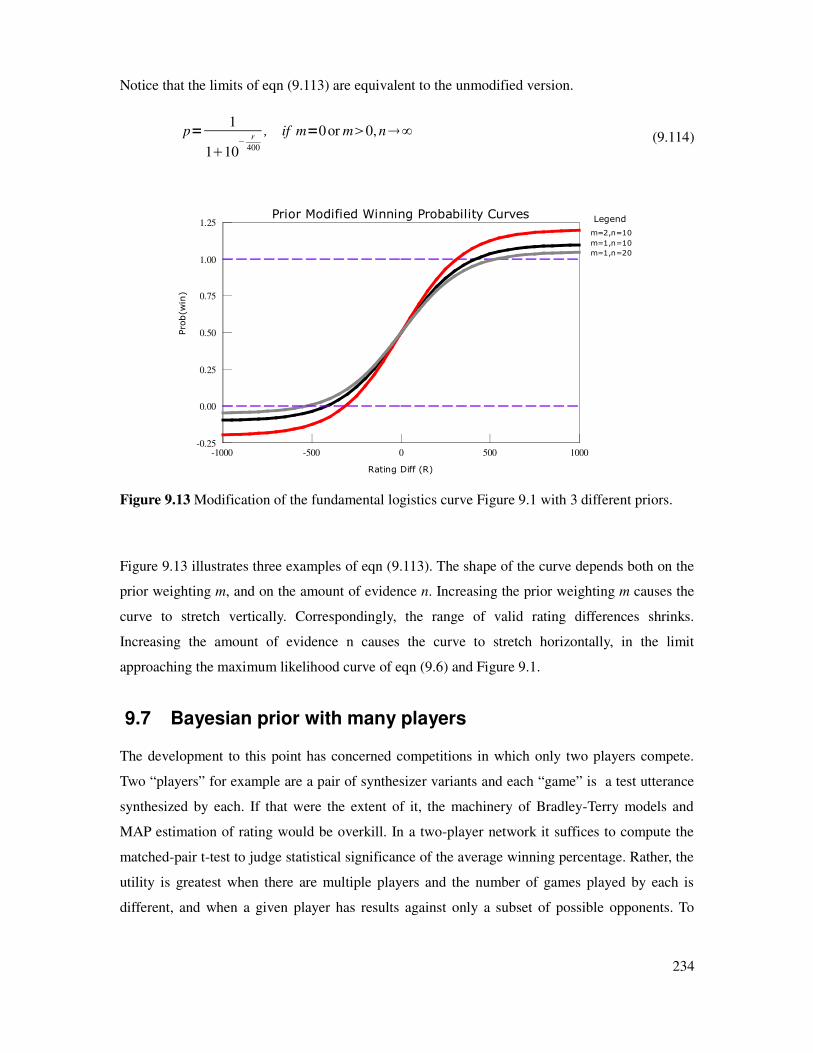
Notice that the limits of eqn (9.113) are equivalent to the unmodified version.

p=1

110−

r

400

, if m=0or m0, n∞ (9.114)

Figure 9.13 Modification of the fundamental logistics curve Figure 9.1 with 3 different priors.

Figure 9.13 illustrates three examples of eqn (9.113). The shape of the curve depends both on the

prior weighting m, and on the amount of evidence n. Increasing the prior weighting m causes the

curve to stretch vertically. Correspondingly, the range of valid rating differences shrinks.

Increasing the amount of evidence n causes the curve to stretch horizontally, in the limit

approaching the maximum likelihood curve of eqn (9.6) and Figure 9.1.

9.7 Bayesian prior with many players

The development to this point has concerned competitions in which only two players compete.

Two “players” for example are a pair of synthesizer variants and each “game” is a test utterance

synthesized by each. If that were the extent of it, the machinery of Bradley-Terry models and

MAP estimation of rating would be overkill. In a two-player network it suffices to compute the

matched-pair t-test to judge statistical significance of the average winning percentage. Rather, the

utility is greatest when there are multiple players and the number of games played by each is

different, and when a given player has results against only a subset of possible opponents. To

234

Rating Diff (R)

-1000 -500 0 500 1000

Prob(w

in)

-0.25

0.00

0.25

0.50

0.75

1.00

1.25Prior Modified Winning Probability Curves Legend

m=2,n=10

m=1,n=10

m=1,n=20

support this more common and realistic situation, we need a way to assign the Bayesian prior in a

network with an unbalance topology. This is accomplished by assigning each player a single

virtual draw and balancing the probability mass amongst all paired comparisons.

Suppose there are m1 players who play a total of N1 games. Let n ij=n ji be the number

of games contested by players i and j. Also ni=∑

i

m nij is the number of games of player i. Then

each link in the network is assigned a weighting ij .

ij = ji=1

2 [n

ij

∑j

m

nij

n

ij

∑i

m

nij ]= 1

2 [ nij

ni

n

ij

n j] (9.115)

ij=

ji=0, if n

ij=0 (9.116)

Then let d 0, d ∈ℝ be the number of virtual draws assigned to each player. This value is

multiplied by ij to determine the prior applied to each linkage.

priorij= prior

ji=d

ij (9.117)

The role of eqn (9.115) is to compute the fraction of games that i plays j, balanced from each

player's side. To provide a small example, suppose there are four players and five games: A vs. B,

A vs. C, A vs. D twice, and B vs. C.

nij=[0 1 1 21 0 1 0

1 1 0 02 0 0 0

] , ni=[42

22] N=

1

2∑i=1

m

ni=5, m=4 (9.118)

nij

ni

=[0 .25 .25 .5.5 0 .5 0

.5 .5 0 01 0 0 0

] (9.119)

ij =[0 .375 .375 .75

.375 0 .5 0

.375 .5 0 0.75 0 0 0

] (9.120)

It can seen that A plays D twice as often as B or C, and the assigned number of virtual draws is

correspondingly doubled. The prior has been redistributed according to the network topology, but

still sums to m when d = 1.

235

∑i

∑j

ij =1

2[∑i

m

∑j

m nij

ni

∑j

m

∑i

m nij

n j]= 1

2 [∑i

m ni

ni

∑j

m nj

n j]= 1

2[mm ]=m (9.121)

In situation of a round-robin, where all players play all, a times each, ij is uniformly distributed.

n ij=a , i≠ j , nij=0, i= j

ij =1

2[n

ij

∑j

m

nij

n

ij

∑i

m

nij ]= 1

2 [ a

a m−1

a

a m−1]= 1

m−1 (9.122)

When m = 2, prior ij=d ij =d , i.e. the degenerate case of adding d virtual draws to each player

in a tournament of two.

9.7.1 Applying player-specific priors

So far, while weighting of the prior is controlled through the parameter d, in a full Bayesian

approach, the prior of each player can be set separately. This is useful if a given player is more

less known than others, and you want to ascribe to this player a greater degree of uncertainty.

This is accomplished by introducing a weighting parameter w. (Determining an appropriate

player-specific weighting on the prior is an important issue, and is perhaps more art than science.)

Continuing the example, one virtual draw is assigned to C and D, two to B, and four to A:

wi

T=[4 211 ] .

nij=[0 1 1 21 0 1 0

1 1 0 02 0 0 0

] , ni=[42

22] , wi=[

42

11] (9.123)

nij

wi

ni

=[0 .25 .25 .5.5 0 .5 0

.5 .5 0 01 0 0 0

][4 2 1 14 2 1 1

4 2 1 14 2 1 1

]=[0 1 1 21 0 1 0

.5 .5 0 01 0 0 0

] (9.124)

ij =[0 1 .75 1.51 0 .75 0

.75 .75 0 01.5 0 0 0

] (9.125)

The effect is that the rating of players with a low w i will be more responsive to actual game

results.

236

9.8 Minorization-Maximization and general EM update

In the analysis of two-player competitions of n games, in which player A beats B k times, we have

P D∣p= pk 1− p n−k under an i.i.d. independence assumption. We want to generalize this

result to m players. The least parsimonious approach is to permit a distinct parameters p ij for

each pairing of players. Let p= pij .

P D∣p =∏i=1

m

∏j=i1

m

pij

k ij1− p ijn ij−kij=∏

i=1

m

∏j= i1

m

pij

k ij p ji

n ij−k ij , p ji =1− pij (9.126)

pij=i

i j

=wij

wijw ji

= pij ,w

ij=wins by i over j

pij=empirical probability(9.127)

This is easy, but doesn't do much good since each pair of players gets their own separate rating

scale. It becomes impossible then to predict the performance of players that have not previously

had an encounter. Instead, each player is assigned a single rating, and the goal is to find the

optimal =i ,2 ,m given the constraints of the game data. In the two-player case:

P D∣ = i

i j

n

j

i j

n−k

(9.128)

= i

i j

w12

j

i j

w 21

, wij=[ 0 k

n−k 0] (9.129)

And in general, for m players, a full product is taken over the win matrix w ij .

P D∣ =∏i=1

m

∏j=1

m

i

i j

w ij

(9.130)

As always log likelihoods provide more fruitful territory.

L D∣ =∑i=1

m

∑j=1

m

wij [ ln i −ln i j ] (9.131)

Unlike eqn (9.66) which could be solved analytically to provide the two-player result pML=k

n ,

the more general case of m players requires an iterative solution. Starting from an initial (random)

setting of =0 an iterative solution generates 0 , 1 k such that the likelihood

increases at each step L k1 L k . To find a parameter update formula for eqn (9.136) it

helps to linearize the nettlesome ln i j term. To make progress, let x=i

j and

237

y=i

k j

k . The term y is a sum based the current estimates of for players i and j, and x is

an updated value that increases the likelihood L . Next we invoke a well known identity of

the logarithm. Due to it being everywhere concave,

ln y−ln x1−x

y, with equality only when x= y (9.132)

−ln x1−x

y− ln y=−

x

y− ln y1 (9.133)

Applying inequality (9.133) to eqn (9.131) with the defined values of x and y creates a proxy

optimization function Qk .

L D∣ =∑i=1

m

∑j=1

m

w ij [ lni −ln x ] , x= i j (9.134)

∑i=1

m

∑j=1

m

w ij[ lni −x

y−ln y1] , y=i

k j

k (9.135)

=∑i=1

m

∑j=1

m

w ij[ lni −

i

j

i

k j

k −ln i

k j

k 1] (9.136)

Qk =∑

i=1

m

∑j=1

m

w ij[ lni −

i

j

i

k j

k −ln i

k j

k 1] (9.137)

Qi

k =∑j=1

m

wij[ lni −

i

j

i

k j

k −ln i

k j

k 1] (9.138)

This proxy optimization function Qk is valuable for two reasons. First is that two functions

are equal at the current estimation point k . The function Qk is said to minorize L at

this point.

L D∣ =Q k D∣ = k minorization point condition (9.139)

L D∣ Q k D∣ , elsewhere (9.140)

Therefore an update function M Q k k1 such that Q k1 ≥Q k implies that

the likelihood function (which is the target objective) will also increase: L k1 ≥L k .

In summary, constructing Qk of (9.137) such that (9.139)-(9.140) hold is the

minorzation step. This is a generalization of the E-step in expectation maximization (EM). Then

updating the parameters k of L through the intermediary function Qk is the

maximization step. This is the same as the M-step in EM.

238

Q k1 ≥Qk maximization step (9.141)

A second advantage of Qk is that it separates the components of the parameter vector .

Thus maximizing eqn (9.137) is equivalent to maximizing eqn (9.138), i.e. of each parameter

component i separately.

A strategy for proving convergence of the set of Bradley-Terry MM algorithms is discussed by

Hunter in [83]. This includes the specific maximization-step of Zermelo [177], formulated in

terms of the fixed-point of the parameter space . Recalling that w ij is the number of wins

player i has over player j, and n ij is the number of games between the two,

i

k1

i

k j

k

i

k

i

k j

k ≃ p ij=w

ij

nij

, as k∞ , for all j≠i (9.142)

the update of k is expressed in terms of the empirical win ratios, in which w i is the total

number of wins by player i.

i

k1=∑

j=1j≠i

m wij

nij

i

k j

k , i

0=

1

m Bradley-Terry maximization step (9.143)

Because each component is optimized separately, the partial results can be used in the current

iteration. Thus eqn (9.143) has a “cyclic” version that is prone to faster convergence.

i

k1=∑

ji

m wij

nij

i

k j

k1 ∑ji

m wij

nij

i

k j

k (9.144)

9.8.1 Small numerical example

In a two-player system application of eqn (9.143) converges after one iteration. Let p be the

winning ratio of player 1, and 10=2

0= 1

2 due to initializing all players to equal ratings.

1

1= p 1

02

0= p 0.50.5 = p

2

1=1− p 1

02

0 =1− p 0.50.5=1− p(9.145)

1

2= p p1− p= p=1

1

2

2=1− p p1− p =1− p=2

1 (9.146)

239

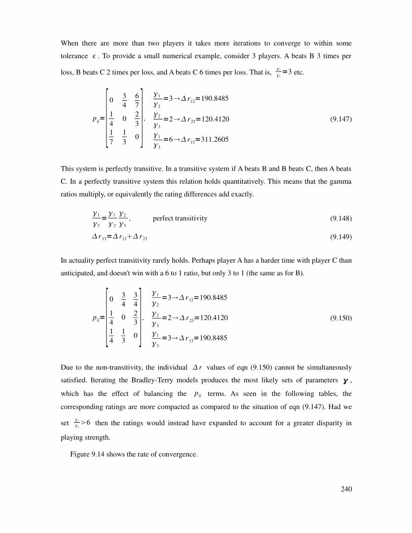
When there are more than two players it takes more iterations to converge to within some

tolerance . To provide a small numerical example, consider 3 players. A beats B 3 times per

loss, B beats C 2 times per loss, and A beats C 6 times per loss. That is, 1

2

=3 etc.

pij=[

03

4

6

7

1

40

2

31

7

1

30 ] ,

1

2

=3 r12=190.8485

2

3

=2 r 23=120.4120

1

3

=6 r13=311.2605

(9.147)

This system is perfectly transitive. In a transitive system if A beats B and B beats C, then A beats

C. In a perfectly transitive system this relation holds quantitatively. This means that the gamma

ratios multiply, or equivalently the rating differences add exactly.

1

3

=1

2

2

3

, perfect transitivity (9.148)

r 13= r12 r23 (9.149)

In actuality perfect transitivity rarely holds. Perhaps player A has a harder time with player C than

anticipated, and doesn't win with a 6 to 1 ratio, but only 3 to 1 (the same as for B).

pij=[0

3

4

3

4

1

40

2

3

1

4

1

30 ] ,

1

2

=3 r 12=190.8485

2

3

=2 r 23=120.4120

1

3

=3 r 13=190.8485

(9.150)

Due to the non-transitivity, the individual r values of eqn (9.150) cannot be simultaneously

satisfied. Iterating the Bradley-Terry models produces the most likely sets of parameters ,

which has the effect of balancing the p ij terms. As seen in the following tables, the

corresponding ratings are more compacted as compared to the situation of eqn (9.147). Had we

set 1

36 then the ratings would instead have expanded to account for a greater disparity in

playing strength.

Figure 9.14 shows the rate of convergence.

240

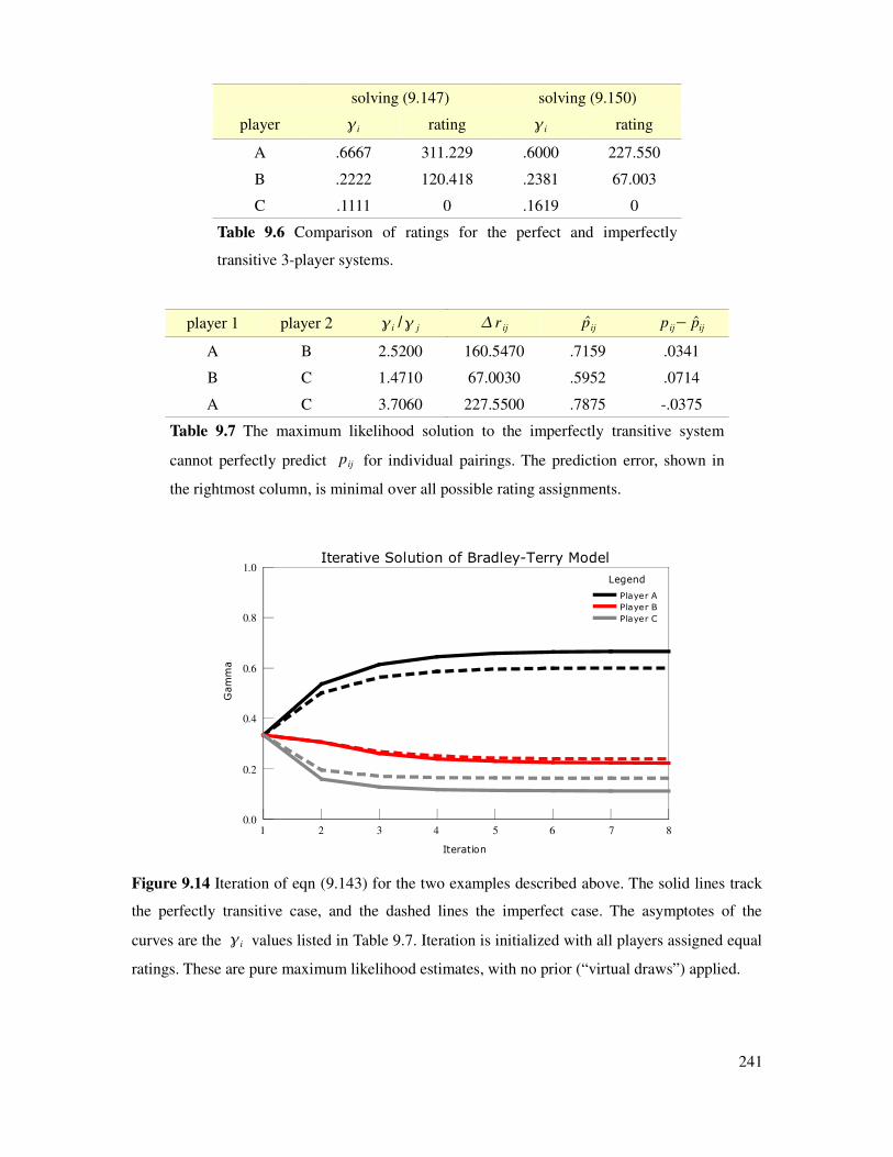
solving (9.147) solving (9.150)

player i rating i rating

A .6667 311.229 .6000 227.550

B .2222 120.418 .2381 67.003

C .1111 0 .1619 0

Table 9.6 Comparison of ratings for the perfect and imperfectly

transitive 3-player systems.

player 1 player 2 i / j r ij pij p ij− pij

A B 2.5200 160.5470 .7159 .0341

B C 1.4710 67.0030 .5952 .0714

A C 3.7060 227.5500 .7875 -.0375

Table 9.7 The maximum likelihood solution to the imperfectly transitive system

cannot perfectly predict pij for individual pairings. The prediction error, shown in

the rightmost column, is minimal over all possible rating assignments.

Figure 9.14 Iteration of eqn (9.143) for the two examples described above. The solid lines track

the perfectly transitive case, and the dashed lines the imperfect case. The asymptotes of the

curves are the i values listed in Table 9.7. Iteration is initialized with all players assigned equal

ratings. These are pure maximum likelihood estimates, with no prior (“virtual draws”) applied.

241

Iteration

1 2 3 4 5 6 7 8

Gamma

0.0

0.2

0.4

0.6

0.8

1.0Iterative Solution of Bradley-Terry Model

Legend

Player A

Player B

Player C

Initializing the iteration with i

0= 1

m is a reasonable first estimate with which to begin. Other

starting points can reduce the number of iterations, but the choice of starting point is not critical.

Because the optimization is convex, convergence is guaranteed and any initial set of gammas will

tend towards the limit point [83]. This can be illustrated the a 3-player of eqn (9.150) because

with three probabilities there are two free parameters ( ∑ii =1 ). The following graph shows the

first couple iterations when the initial values lie on the edge of the parameters space.

Experimentally, in this small system about 12-15 iterations are required for ∑i∣

i

k1−i

k ∣

where the stopping tolerance is =10−6 .

Figure 9.15 Convergence of 1 and 2 when the initial estimate in these dimensions lies on the

edge of the parameter space. The convergence point is (0.6, 0.2381, 0.1619).

242

γ1

0.0 0.2 0.4 0.6 0.8 1.0

γ 2

0.0

0.2

0.4

0.6

0.8

1.0Gamma Convergence

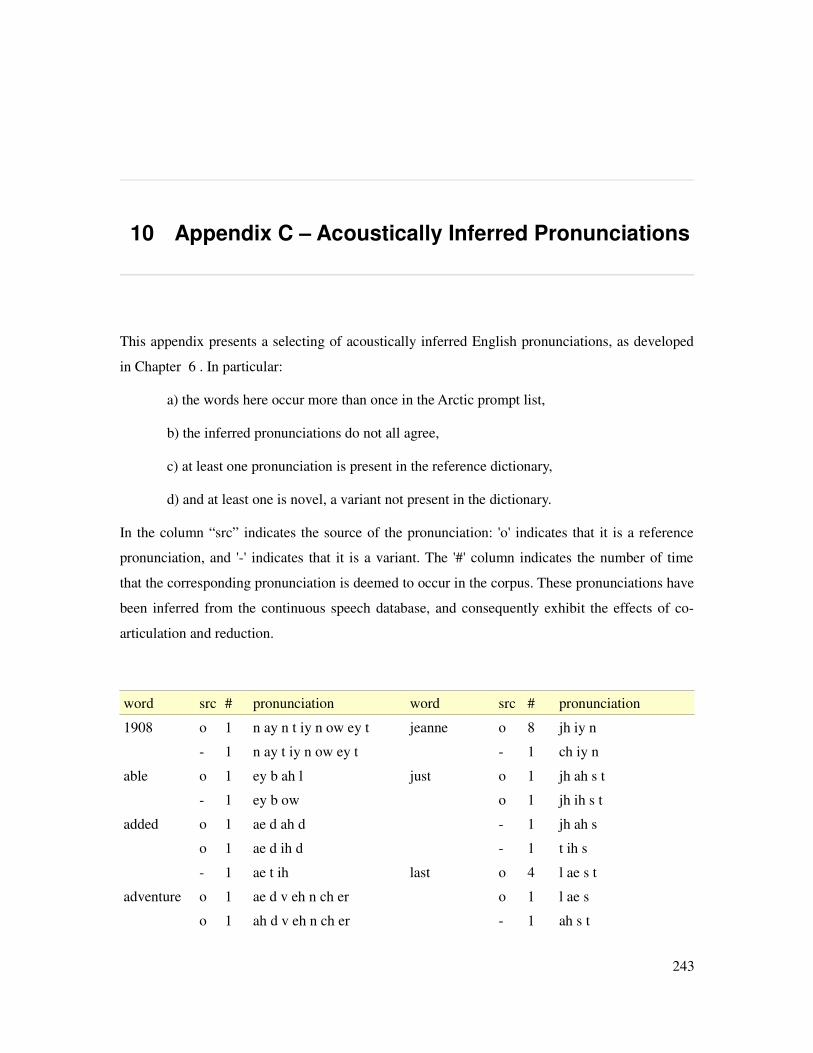
10 Appendix C – Acoustically Inferred Pronunciations

This appendix presents a selecting of acoustically inferred English pronunciations, as developed

in Chapter 6 . In particular:

a) the words here occur more than once in the Arctic prompt list,

b) the inferred pronunciations do not all agree,

c) at least one pronunciation is present in the reference dictionary,

d) and at least one is novel, a variant not present in the dictionary.

In the column “src” indicates the source of the pronunciation: 'o' indicates that it is a reference

pronunciation, and '-' indicates that it is a variant. The '#' column indicates the number of time

that the corresponding pronunciation is deemed to occur in the corpus. These pronunciations have

been inferred from the continuous speech database, and consequently exhibit the effects of co-

articulation and reduction.

word src # pronunciation word src # pronunciation

1908 o 1 n ay n t iy n ow ey t jeanne o 8 jh iy n

- 1 n ay t iy n ow ey t - 1 ch iy n

able o 1 ey b ah l just o 1 jh ah s t

- 1 ey b ow o 1 jh ih s t

added o 1 ae d ah d - 1 jh ah s

o 1 ae d ih d - 1 t ih s

- 1 ae t ih last o 4 l ae s t

adventure o 1 ae d v eh n ch er o 1 l ae s

o 1 ah d v eh n ch er - 1 ah s t

243

- 1 ih d f eh n ch er left o 2 l eh f t

again o 3 ah g eh n - 1 ae f t

- 1 ey g eh n letter o 2 l eh t er

- 1 ih g eh n - 1 m eh d er

against o 2 ah g eh n s t life o 8 l ay f

- 1 ih k ae n s t - 1 ay f

ago o 3 ah g ow like o 12 l ay k

- 1 ih k ow - 2 ay k

almost o 4 ao l m ow s t - 2 l ay

- 1 ao l m ow s - 1 l ay t

along o 1 ah l ao ng - 1 w ay k

- 1 ng l ao ng - 1 d ay k

- 1 l ao ng - 1 v ay k

already o 7 ao l r eh d iy lived o 2 l ih v d

- 1 ao l r eh d ey - 1 ah v d

- 1 l r eh d iy - 1 ih v

an o 10 ae n living o 1 l ih v ih ng

o 6 ah n - 1 ih v ih ng

- 1 w ah n looking o 1 l uh k ih ng

- 1 ih n - 1 l uh k ih n

- 1 eh n lop o 1 l aa p

and o 60 ae n d - 1 l aa b

- 29 ae n lost o 2 l ao s t

o 26 ah n d - 1 l aa s

- 6 ih n macdougall o 1 m ah k d uw g ah l

- 3 eh n d - 1 m ih k d uw g aa l

- 3 ah n - 1 t uw g ow

- 2 eh n made o 9 m ey d

- 1 ae n y uw - 1 m ey

- 1 ih ng make o 2 m ey k

- 1 ae m - 1 m ey d

- 1 ah m minute o 1 m ih n ah t

- 1 ae t - 1 m eh n ae t

anything o 4 eh n iy th ih ng moment o 5 m ow m ah n t

- 1 ae n iy th ih ng - 1 m ow m eh n t

244

appearance o 1 ah p ih r ah n s - 1 m ow m ah d

- 1 p ih r n s much o 6 m ah ch

aroused - 1 er ae l s t - 1 m aa ch

o 1 er aw z d my o 31 m ay

- 1 r aw s t - 1 b ay

articulate o 1 aa r t ih k y ah l ah t night o 3 n ay t

- 1 er t ih k ey l ay t - 1 n ay

as o 20 ae z nodded o 1 n aa d ah d

- 2 ih s - 1 n aa t eh d

- 1 ah z not o 26 n aa t

- 1 ah s - 1 n aa t k

aside o 1 ah s ay d - 1 aa t

- 1 eh s ay d now o 19 n aw

asked o 1 ae s t - 1 n ow

- 1 ae s k o'brien - 2 ow b r ay n

asleep o 1 ah s l iy p o 1 ow b r ay ih n

- 1 s l iy p - 1 w b r ay n

at o 23 ae t occurred o 3 ah k er d

- 1 ih t - 1 ih k er

- 1 eh t of o 116 ah v

- 1 ah p - 1 ih v

- 1 ah d - 1 ao v

- 1 ay t on o 14 aa n

ate o 2 ey t o 2 ao n

- 1 ey d - 2 ah n

attempt o 1 ah t eh m p t one o 11 w ah n

- 1 ah t eh m t o 1 hh w ah n

attempted o 1 ah t eh m p t ah d - 1 w aa n

- 1 n t eh m p t ih d - 1 w ah

away o 2 ah w ey - 1 ah n

- 1 ow w ey or o 6 ao r

- 1 iy w ey - 1 ih n

- 1 w ey our - 3 er

back o 7 b ae k o 2 aw er

- 1 d ae k o 2 aa r

245

be o 16 b iy - 1 w er

- 1 p iy ourselves - 3 er s eh l v z

began o 5 b ih g ae n o 2 aw er s eh l v z

- 1 b ih k ae n o 1 aa r s eh l v z

believe o 2 b ih l iy v - 1 eh r s eh l v z

- 1 b ih l iy f - 1 ao r s eh l v z

beyond o 2 b ih aa n d outrageous o 1 aw t r ey jh ah s

- 2 b iy aa n - 1 aw t r ey jh ih s

- 1 p iy aa n dh over o 6 ow v er

- 1 b iy aa n dh - 1 v er

big o 6 b ih g passed o 2 p ae s t

- 1 p ih g - 1 b ae s t

- 1 p ey g - 1 p ae s

black o 1 b l ae k people o 1 p iy p ah l

- 1 b ay k - 1 p iy p ow l

both o 3 b ow th - 1 p iy p ao l

- 1 b oy dh per o 2 p er

burned o 1 b er n d - 1 p r

- 1 b er n perrault o 1 p er ao l t

but o 20 b ah t - 1 p r ow

- 3 b ah phil o 1 f ih l

by o 17 b ay - 1 f eh l

- 1 p ay pierre's - 1 p iy eh r ih z

cabin o 2 k ae b ah n o 1 p iy eh r z

- 1 k ae b ih n place o 1 p l ey s

- 1 k ae b n - 1 p l ey z

came o 4 k ey m pointing o 1 p oy n t ih ng

- 1 k iy m - 1 p oy n t iy n

can o 3 k ae n pounds o 1 p aw n z

- 1 k ih n d - 1 p aw n s

- 1 k ih n read o 1 r eh d

can't - 2 k ae n - 1 r iy

o 1 k ae n t resemblance o 2 r ih z eh m b l ah n s

captain o 1 k ae p t ah n - 1 r ah z eh m b l ah n s

- 1 k ae p t ih n room o 1 r uw m

246

children o 2 ch ih l d r ah n - 1 r eh m

- 1 ch ih l b ah n rush o 2 r ah sh

closed o 2 k l ow z d - 1 r eh sh

- 1 k l ow z saw o 11 s ao

come o 4 k ah m - 4 s aa

- 1 k aa m scrap o 1 s k r ae p

- 1 k iy w - 1 k r ae p

- 1 k aa seemed o 4 s iy m d

coming o 2 k ah m ih ng - 1 s iy m

- 1 k ah m ey n singing o 1 s ih ng ih ng

continue o 1 k ah n t ih n y uw - 1 s ih ng ng

- 1 k ih n t ih n y uw slightest o 1 s l ay t ah s t

continued o 2 k ah n t ih n y uw d - 1 s l ih t ih s

- 1 k ih n t ey n y uw d some o 2 s ah m

- 1 k ih n t eh n y uw - 1 z aa n

- 1 t t iy sound o 3 s aw n d

destroy o 1 d ih s t r oy - 1 aw n d

- 1 iy s t r oy started o 1 s t aa r t ah d

did o 10 d ih d - 1 s t aa r d ih t

- 1 d eh d stepped o 1 s t eh p t

die o 2 d ay - 1 s t ah p

- 1 g ay strange o 4 s t r ey n jh

do o 7 d uw - 1 t r ey n jh

- 1 t uw sure o 3 sh uh r

- 1 t iy - 1 ch er

down o 6 d aw n test o 1 t eh s t

- 1 t aw n - 1 eh s t

dreams o 2 d r iy m z than o 6 dh ae n

- 1 t r iy m z o 2 dh ah n

each o 4 iy ch - 2 dh eh n

- 1 hh iy ch - 1 th n

eileen o 2 ay l iy n that o 36 dh ae t

- 1 ey l iy n o 2 dh ah t

even - 1 hh iy v ih n - 2 d ae t

o 1 iy v ih n - 2 ae t

247

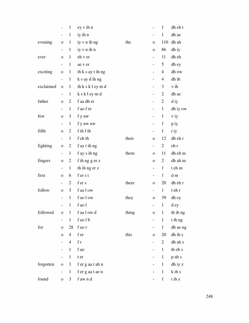
- 1 ey v ih n - 1 dh eh t

- 1 iy ih n - 1 dh ae

evening o 1 iy v n ih ng the o 110 dh ah

- 1 iy v n ih n o 86 dh iy

ever o 1 eh v er - 11 dh eh

- 1 ae v er - 5 dh ey

exciting o 1 ih k s ay t ih ng - 4 dh ow

- 1 k s ay d ih ng - 4 dh ih

exclaimed o 1 ih k s k l ey m d - 3 v ih

- 1 k s k l ey m d - 2 dh ae

father o 2 f aa dh er - 2 d iy

- 1 f ao f er - 1 dh iy ow

few o 3 f y uw - 1 v iy

- 1 f y uw uw - 1 p iy

fifth o 2 f ih f th - 1 t iy

- 1 f eh th their o 12 dh eh r

fighting o 2 f ay t ih ng - 2 eh r

- 1 f ay s ih ng them o 11 dh eh m

fingers o 2 f ih ng g er z o 2 dh ah m

- 1 th ih ng er z - 1 t eh m

first o 6 f er s t - 1 d m

- 2 f er s there o 20 dh eh r

follow o 3 f aa l ow - 1 t eh r

- 1 f ao l ow they o 39 dh ey

- 1 f ao l - 1 d ey

followed o 1 f aa l ow d thing o 1 th ih ng

- 1 f ao l b - 1 t ih ng

for o 28 f ao r - 1 dh ae ng

o 4 f er this o 20 dh ih s

- 4 f r - 2 dh ah s

- 1 f ao - 1 th eh s

- 1 t er - 1 p ah s

forgotten o 3 f er g aa t ah n - 1 dh iy z

- 1 f er g aa t ae n - 1 k ih s

found o 3 f aw n d - 1 t ih z

248

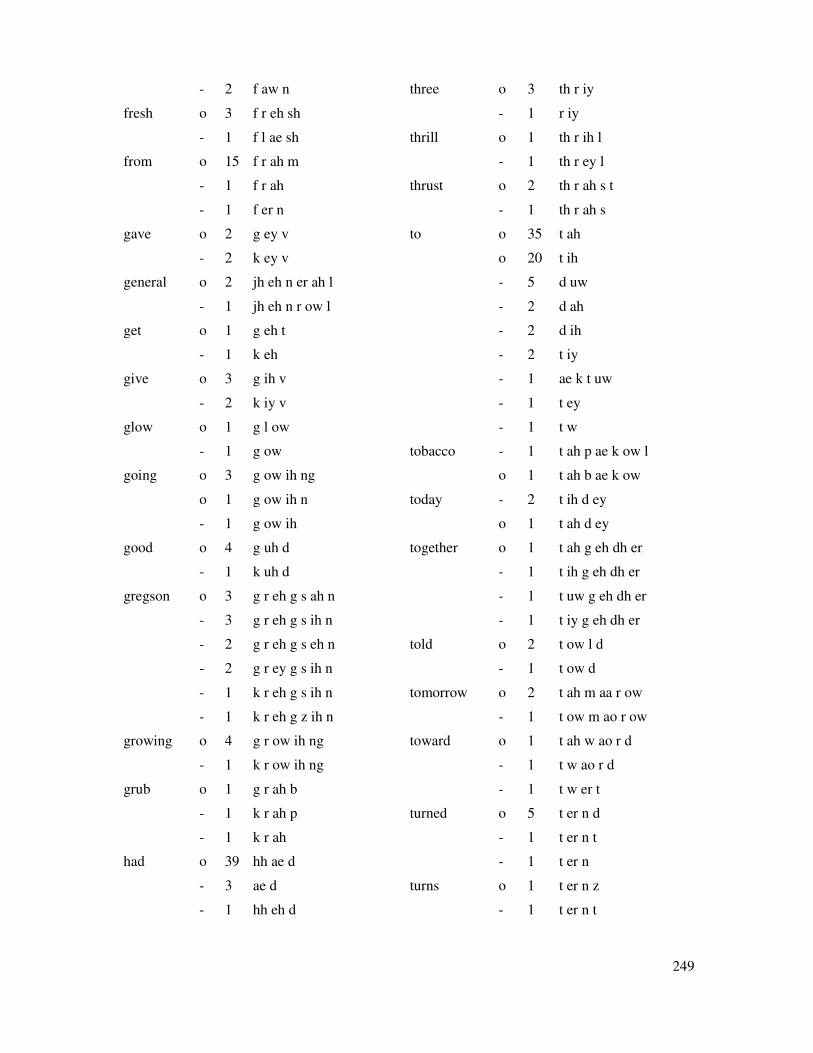
- 2 f aw n three o 3 th r iy

fresh o 3 f r eh sh - 1 r iy

- 1 f l ae sh thrill o 1 th r ih l

from o 15 f r ah m - 1 th r ey l

- 1 f r ah thrust o 2 th r ah s t

- 1 f er n - 1 th r ah s

gave o 2 g ey v to o 35 t ah

- 2 k ey v o 20 t ih

general o 2 jh eh n er ah l - 5 d uw

- 1 jh eh n r ow l - 2 d ah

get o 1 g eh t - 2 d ih

- 1 k eh - 2 t iy

give o 3 g ih v - 1 ae k t uw

- 2 k iy v - 1 t ey

glow o 1 g l ow - 1 t w

- 1 g ow tobacco - 1 t ah p ae k ow l

going o 3 g ow ih ng o 1 t ah b ae k ow

o 1 g ow ih n today - 2 t ih d ey

- 1 g ow ih o 1 t ah d ey

good o 4 g uh d together o 1 t ah g eh dh er

- 1 k uh d - 1 t ih g eh dh er

gregson o 3 g r eh g s ah n - 1 t uw g eh dh er

- 3 g r eh g s ih n - 1 t iy g eh dh er

- 2 g r eh g s eh n told o 2 t ow l d

- 2 g r ey g s ih n - 1 t ow d

- 1 k r eh g s ih n tomorrow o 2 t ah m aa r ow

- 1 k r eh g z ih n - 1 t ow m ao r ow

growing o 4 g r ow ih ng toward o 1 t ah w ao r d

- 1 k r ow ih ng - 1 t w ao r d

grub o 1 g r ah b - 1 t w er t

- 1 k r ah p turned o 5 t er n d

- 1 k r ah - 1 t er n t

had o 39 hh ae d - 1 t er n

- 3 ae d turns o 1 t er n z

- 1 hh eh d - 1 t er n t

249

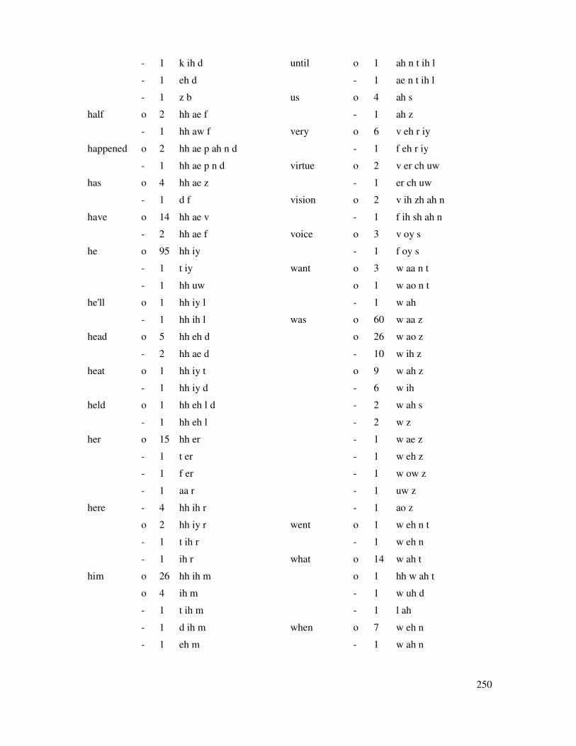
- 1 k ih d until o 1 ah n t ih l

- 1 eh d - 1 ae n t ih l

- 1 z b us o 4 ah s

half o 2 hh ae f - 1 ah z

- 1 hh aw f very o 6 v eh r iy

happened o 2 hh ae p ah n d - 1 f eh r iy

- 1 hh ae p n d virtue o 2 v er ch uw

has o 4 hh ae z - 1 er ch uw

- 1 d f vision o 2 v ih zh ah n

have o 14 hh ae v - 1 f ih sh ah n

- 2 hh ae f voice o 3 v oy s

he o 95 hh iy - 1 f oy s

- 1 t iy want o 3 w aa n t

- 1 hh uw o 1 w ao n t

he'll o 1 hh iy l - 1 w ah

- 1 hh ih l was o 60 w aa z

head o 5 hh eh d o 26 w ao z

- 2 hh ae d - 10 w ih z

heat o 1 hh iy t o 9 w ah z

- 1 hh iy d - 6 w ih

held o 1 hh eh l d - 2 w ah s

- 1 hh eh l - 2 w z

her o 15 hh er - 1 w ae z

- 1 t er - 1 w eh z

- 1 f er - 1 w ow z

- 1 aa r - 1 uw z

here - 4 hh ih r - 1 ao z

o 2 hh iy r went o 1 w eh n t

- 1 t ih r - 1 w eh n

- 1 ih r what o 14 w ah t

him o 26 hh ih m o 1 hh w ah t

o 4 ih m - 1 w uh d

- 1 t ih m - 1 l ah

- 1 d ih m when o 7 w eh n

- 1 eh m - 1 w ah n

250

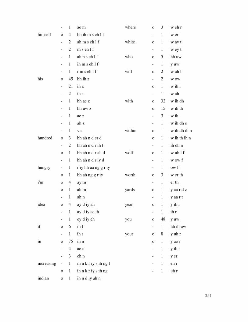
- 1 ae m where o 3 w eh r

himself o 4 hh ih m s eh l f - 1 w er

- 2 ah m s eh l f white o 1 w ay t

- 2 m s eh l f - 1 w ey t

- 1 ah n s eh l f who o 5 hh uw

- 1 ih m s eh l f - 1 y uw

- 1 r m s eh l f will o 2 w ah l

his o 45 hh ih z - 2 w ow

- 21 ih z o 1 w ih l

- 2 ih s - 1 w ah

- 1 hh ae z with o 32 w ih dh

- 1 hh uw z o 15 w ih th

- 1 ae z - 3 w ih

- 1 ah z - 1 w ih dh s

- 1 v s within o 1 w ih dh ih n

hundred o 3 hh ah n d er d o 1 w ih th ih n

- 2 hh ah n d r ih t - 1 ih dh n

o 1 hh ah n d r ah d wolf o 1 w uh l f

- 1 hh ah n d r iy d - 1 w ow f

hungry - 1 r iy hh aa ng g r iy - 1 ow f

o 1 hh ah ng g r iy worth o 3 w er th

i'm o 4 ay m - 1 er th

o 1 ah m yards o 1 y aa r d z

- 1 ah n - 1 y aa r t

idea o 4 ay d iy ah year o 1 y ih r

- 1 ay d iy ae th - 1 ih r

- 1 ey d iy eh you o 48 y uw

if o 6 ih f - 1 hh ih uw

- 1 ih t your o 8 y uh r

in o 75 ih n o 1 y ao r

- 4 ae n - 1 y ih r

- 3 eh n - 1 y er

increasing - 1 ih n k r iy s ih ng l - 1 eh r

o 1 ih n k r iy s ih ng - 1 uh r

indian o 1 ih n d iy ah n

251

- 1 n d iy ah n

into o 11 ih n t uw

- 1 n t uw

is o 29 ih z

- 1 w aa z

it o 55 ih t

- 5 ae t

- 2 eh t

- 1 ah t

- 1 ah d

- 1 ah p

- 1 d s

its o 8 ih t s

- 1 t s

252

11 Appendix D – The Three Laws of Disserosophy

As conveyed by (Collins-Thompson, 2008) [97].

1. A good dissertation is a finished dissertation.

2. No dissertation is ever finished... merely abandoned.

3. Anyway, only ten people in the world will ever read it.

253

254

12 Bibliography

[1] Afrikaans 37k lexicon. CMU internal datafile, 2005.

[2] American Heritage Dictionary of the English Language. Houghton Mifflin Company,

2006.

[3] Andersen, Ove, Kuhn, Roland, Lazarides, Ariane, Dalsgaard, Paul, Haas, Jurgen & Noth,

Elmar. Comparison of Two Tree-Structured Approaches for Grapheme-to-Phoneme

Conversion. In The 4th International Conference on Spoken Language Processing

(ICSLP, Philadelpha, PA, USA), 1996.

[4] Anumanchipalli, Gopala Krishna. Modeling Pronunciation Variation for Speech

Recognition. Masters Thesis, Language Technologies Research Center, International

Institute of Information Technology, Hyderabad, India. 2008.

[5] Anumanchipalli, Gopala Krishna, Prahallad, Kishore & Black, Alan W. Significance of

Early Tagged Contextual Graphemes in Grapheme Based Speech Synthesis and Speech

Recognition Systems. In Proceedings of IEEE International Conference on Acoustics,

Speech and Signal Processing (ICASSP, Las Vegas, USA), 2008.

[6] Appen Iraqi Pronunciation Dictionary (product code ARB_LEX004),

http://www.appen.com.au, 2008.

[7] Bacchiani, Michiel & Ostendorf, Mari. Design of a speech recognition system based on

non-uniform segmental units. In Proceedings of the International Conference on

Acoustics, Speech and Signal Processing (ICASSP, Atlanta, GA, USA), 1996.

[8] Bacchiani, Michiel, Ostendorf, Mari, Sagisaka, Y & Paliwal, K. Using Automatically-

Derived Acoustic Subword Units in Large Vocabulary Speech Recognition. In The 5th

International Conference on Spoken Language Processing (ICSLP, Sydney, Australia),

1998.

[9] Bacchiani, Michiel. Speech Recognition System Design Based on Automatically Derived

255

Units. PhD dissertation, Boston University College of Engineering, 1999.

[10] Bacchiani, Michiel. Joint Lexicon Acoustic Unit Inventory and Model Design, Speech

Communication, Elsevier, vol.29, no.2-4, 1999.

[11] Bach, N, Eck, M, Charoenpornsawat, P, Koehler, T, Strueker, S & Nygen, T. The CMU

TransTac 2007 Eyes-free and Hands-free two-way Speech-to-Speech Translation System.

In 4th International Workshop on Spoken Language Translation (IWSLT, Trento, Italy),

2007.

[12] Badino, Leonardo, Barolo, Claudia & Quazza, Silvia. Language Independent Phoneme

Mapping for Foreign TTS. In 5th ISCA Speech Synthesis Workshop (Pittsburgh, PA,

USA), 2005.

[13] Bahl, L R, Das, S, deSouza, P V, Epstein, M, Mercer, R L, Merialdo, B, Nahamoo, D,

Picheny, M & Powell, J. Automatic Phonetic Baseform Determination. In Proceedings of

the Workshop on Speech and Natural Language, 1990.

[14] Barry, W J & Fourcin, AJ. Levels of Labeling. Computer Speech and Language (1992)

vol 6, pp. 1-14.

[15] BayesElo. http://remi.coulom.free.fr/Bayesian-Elo/.

[16] Bellegarda, Jerome R. Unsupervised, Language-Independent Grapheme-to-Phoneme

Conversion by Latent Analogy. Speech Communication (2005), vol. 46, no. 2, pp. 140-

152.

[17] Bellegarde, Jerome R. Latent Semantic Mapping. IEEE Signal Processing Magazine

(2005), vol. 22, no. 5, pp. 70-80.

[18] Black, Alan W, Lenzo, Kevin & Pagel, Vincent. Letter to Sound Rules for Accented

Lexicon Compression. In The 5th International Conference on Spoken Language

Processing (ICSLP98, Syndey, Australia), 1998.

[19] Black, Alan W, Lenzo, Kevin & Pagel, Vincent. Issues in Building General Letter to

Sound Rules. In 3rd ESCA Workshop on Speech Synthesis (Jenolan Caves, Australia),

1998.

[20] Black, Alan W & Lenzo, Kevin. Limited Domain Synthesis. In Proceedings of the

International Conference on Acoustics, Speech and Signal Processing (ICSLP, Bejing,

China), 2000.

[21] Black, Alan W & Font Llitjos, Ariadna. Unit Selection Without a Phoneme Set. In IEEE

TTS Workshop 2002 (Santa Monica, CA), 2002.

[22] Black, Alan W & Lenzo, Kevin. Multilingual Text-to-Speech Synthesis. In Proceedings

of the International Conference on Acoustics, Speech and Signal Processing (ICASSP,

256

Montreal, Canada), 2004.

[23] Black, Alan W & Schultz, Tanja. Speaker Clustering for Multilingual Synthesis. In

Proceedings of the ISCA Tutorial and Research Workshop on Multilingual Speech and

Language Processing (Stellenbosch, South Africa), 2006.

[24] Black, Alan W. CLUSTERGEN: A Statistical Parametric Synthesizer using Trajectory

Modeling. In Interspeech 2006 (ICSLP, Pittsburgh, PA, USA), 2006.

[25] Black, Alan, Zen, Heiga & Tokuda, Keiichi. Statistical Parametric Synthesis. In

Proceedings of the International Conference on Acoustics, Speech and Signal Processing

(ICAASP, Honolulu, Hawai'i), 2007.

[26] Black, Alan W & Tokuda, Keiichi. The Blizzard Challenge – 2005: Evaluating Corpus-

Based Speech Synthesis on Common Datasets. In Interspeech Special Session - Blizzard

Challenge (EuroSpeech, Lisbon, Portugal), 2005.

[27] Black, Alan W, Tokuda, Keiichi, King, Simon, Hirai, T, Picheny, M & Nakamura, S.

Blizzard Challenge – 2006. In Interspeech 2006 Satellite Workshop (ICSLP, Pittsburgh,

PA, USA), 2006.

[28] Fraser, Mark & King, Simon. The Blizzard Challenge 2007. In Workshop in Conjunction

with 6th ISCA Workshop on Speech Synthesis (Bonn, Germany), 2007.

[29] Karaiskos, Vasilis, King, Simon, Clark, Robert & Mayo, Catherine. In The Blizzard

Challenge 2008 workshop in Conjunction with Interspeech 2008 (Brisbane, Australia),

2008.

[30] Bradley, R A & Terry, ME. Rank Analysis of Incomplete Block Designs. I. The method of

paired comparisons. Biometrica (1952), vol. 39, pp. 324-345.

[31] Breiman, Leo, Freidman, Jerome, Stone, Charles J & Olshen, RA. Classification and

Regression Trees. Chapman & Hall, 1984.

[32] Bright, W, et al. International Encyclopedia of Linguistics. Bright W. (Ed.). Oxford

University Press, 1992.

[33] Brown, Peter, Pietra, Stephen A, Pietra, Vincent J & Mercer, Robert L. Statistical

Machine Translation: The IBM Translation Models 1-3. (2006).

[34] Buckwalter Arabic Transliteration. http://www.qamus.org/transliteration.htm/.

[35] Campbell, Nick. Talking Foreign – Concatenative Speech Synthesis and Language

Barrier. In 7th European Conference on Speech Communication and Technology

(EuroSpeech, Aalborg, Denmark), 2001.

[36] CELEX . Baayen, R H, Piepenbrock, R & Gulikers, L. The CELEX Lexical Database

(Release 2) [CD-ROM]. Philadelphia, PA: Linguistic Data Consortium, University of

257

Pennsylvania [Distributor], 1995.

[37] Cepstral Inc. www.cepstral.com.

[38] Černocký, Jan, Baudoin, Geneviève & Chollet, Gérard. Speech Processing Using

Automatically Derived Segmental Units: towards an ALISP-based Recognizer. In

Technical Annex Cost 249 meeting (Praha, Czech Republic), 1999.

[39] Chomsky, Noam & Halle, Morris. The Sound Patterns of English. MIT Press, 1968.

[40] Chotimongkol, Ananlada & Black, Alan W. Statistically Trained Orthographic to Sound

Models for Thai. In Proceedings of the 6th International Conference on Spoken

Language Processing (ICSLP, Beijing, China), 2000.

[41] CMU ARCTIC Single Speaker Speech Databases. www.festvox.org/cmu_arctic.

[42] Carnegie Mellon Pronouncing Dictionary. http://www.speech.cs.cmu.edu/cgi-

bin/cmudict/.

[43] Comrie, B, et al. The World's Major Languages. Comrie B (ed.). Oxford University

Press, 1990.

[44] Cosi, P, Gretter, R & Tesser, F. Festival Parla Italiano. In Proceedings of GFS2000, xi

giornate del gruppo di fonetica sperimentale (Padova, Italy), 2000.

[45] Das, Gurchan. India Unbound: The Social and Economic Revolution from Independence

to the Global Information Age. Anchor, 2002.

[46] Davel, Marelie & Barnard, Etienne. Bootstrapping in Language Resource Generation. In

Proceedings of the 14th Pattern Recognition Association of South Africa (Langebaan,

South Africa), 2003.

[47] Davel, Marelie & Barnard, Etienne. The Efficient Generation of Pronunciation

Dictionaries: Machine Learning Factors during Bootstrapping. In Interspeech 2004 (Jeju

Island, Korea), 2004.

[48] Davel, Marelie & Barnard, Etienne. The Efficient Generation of Pronunciation

Dictionaries: Human Factors during Bootstrapping. In Interspeech 2004 (Jeju Island,

Korea), 2004.

[49] Davel, Marelie & Barnard, Etienne. A default-and-refinement approach to pronunciation

prediction. In 15th symposium of the Pattern Recognition Association of South Africa

(Grabouw, South Africa), 2004.

[50] Davel, Marelie & Barnard, Etienne. Bootstrapping Pronunciation Dictionaries: Practical

Issues. In Interspeech 2004 (EuroSpeech, Lisbon, Portugal), 2004.

[51] Davel, Marelie Hattingh. Pronunciation Modelling and Bootstrapping. PhD dissertation,

University of Pretoria, 2005.

258

[52] Davel, Marelie & Barnard, Etienne. Bootstrapping for the efficient development of

pronunciation dictionaries, In Transactions of the SAIEE: Special Issue on Pattern

Recognition: Theory and Applications, 2005.

[53] Davel, Marelie & Barnard, Etienne. Obtaining a Minimal Set of Rewrite Rules. In

Proceedings of the 16th Annual Symposium of the Pattern Recognition Association of

South Africa (Langebaan, South Africa), 2005.

[54] Davel, Marelie & Barnard, Etienne. Extracting Pronunciation Rules for Phonemic

Variants. In ISCA Tutorial and Research Workshop (Stellenbosch, South Africa), 2006.

[55] Davel, Marelie & Barnard, Etienne. Developing consistent pronunciation variants. In

Interspeech 2006 (ICSLP, Pittsburgh, PA, USA), 2006.

[56] Davel, Marelie & Barnard, Etienne. Effort and Accuracy during Language Resource

Generation: a Pronunciation Prediction Case Study. In Proceedings of the 17th Annual

Symposium of the Pattern Recognition Association of South Africa (Parys, South Africa),

2006.

[57] Davel, Marelie & Barnard, Etienne. Bootstrapping Pronunciation Dictionaries, South

African Journal of Science, 2006.

[58] Davel, Marelie & Barnard, Etienne. Effort and Accuracy during Language Resource

Generation: A Pronunciation Prediction Case Study, SAIEE Africa Research Journal,

vol.98, no.4, 2007.

[59] Davel, Marelie & Barnard, Etienne. Pronunciation predication with Default & Refine,

Computer Speech and Language, vol.22, 2008.

[60] DeCloet, Derek. Now it's India Rising. Toronto Globe & Mail, Feb. 17 2007.

[61] Dempster, A P, Laird, N M & Rubin, D B. Maximum Likelihood from Incomplete Data

via the EM algorithm. In J. Royal Statistical Society Series B, 1977.

[62] Deutscher, Guy. The Unfolding of Language: An Evolutionary Tour of Mankind's

Greatest Invention. Metropolitan Books, 2005.

[63] DictionaryMaker. http://sourceforge.net/projects/dictionarymaker/.

[64] Divay, Michel & Vitale, Anthony J. Algorithms for Grapheme-Phoneme Translation for

English and French: Applications for Database Searches and Speech Synthesis.

Computational Linguistics (1997), vol 23, no. 4, pp. 495-523.

[65] The Edinburgh Speech Tools Library. http://www.cstr.ed.ac.uk/projects/speech_tools/.

[66] Elo, Arpad. The Rating of Chess Players Past and Present. Arco, New York, 1978.

[67] Engelbrecht, Herman & Schultz, Tanja. Rapid Development of an Afrikaans-English

Speech-to-Speech Translator. In Proceedings of International Workshop on Spoken

259

Language Translation (IWSLT, Pittsburgh, PA), 2005.

[68] Ethnologue: Languages of the World. Gordon, Raymond G., Jr. (ed.). SIL International,

2005.

[69] Festival. Black, Alan W, Caley, Richard, Taylor, Paul.

http://www.cstr.ed.ac.uk/projects/festival/.

[70] Festvox. Black, Alan W, Lenzo, Kevin. http://www.festvox.org/.

[71] FIDE. http://ratings.fide.com/calculators.phtml.

[72] Finke, M, Geutner, P, Hild, H, Kemp, T, Ries, K & Westphal, M. The Karlsruhe

Verbmobil Spech Recognition Engine. In Proceedings of the International Conference on

Acoustics, Speech and Signal Processing (ICASSP, Munich, Germany), 1997.

[73] Flite. Black, Alan W. http://www.speech.cs.cmu.edu/flite/.

[74] Fonilex. Mertens, Piet & Vercammen, Filip. Fonilex: a Pronunciation Database of Dutch

in Flanders. 1998.

[75] Gakuru, Mucemi, Iraki, Frederick K, Tucker, Roger, Shalonova, Ksenia & Ngugi,

Kamanda. Development of a Kiswahili Text To Speech System. In Interspeech 2005

(EuroSpeech, Lisbon, Portugal), 2005.

[76] Giridharadas, Anand. India Economy Grows at Torrid Pace. New York Times, Sept. 29

2006.

[77] Graff, David, Maamouri, Mohamed, Zaghouani, Wajdi, Ateyah, Luma & Ismael.

Expanding the Iraqi Arabic Grammatical Lexicon (IAGL). In Transtac PI Meeting (Nov

14), 2007.

[78] Project Gutenberg. http://www.gutenberg.org/wiki/Main_Page/.

[79] Hakkani-tür, Dilek & Gorin, Allen. Active Learning for Automatic Speech Recognition.

In Proceedings of the International Conference on Acoustics, Speech and Signal

Processing (ICASSP, Orlando, FL, USA), 2002.

[80] Harvey, Fiona. Computers for the Third World: the Simputer is a handheld device

designed for rural villagers. Scientific American, September, 2002.

[81] HealthLine. http://www.cs.cmu.edu/~healthline/.

[82] Huang, Xuedong, Acero, Alex & Hon, Hsiao-Wuen. Spoken Language Understanding: a

Guide to Theory, Algorithm, and System Development. Prentice Hall, 2001.

[83] Hunter, David R. MM Algorithms for Generalized Bradley-Terry Models. The Annals of

Statistics (2004), vol. 32, no. 1, pp. 384-406.

[84] IPA. Handbook of the International Phonetic Association: A Guide to the Use of the

International Phonetic Alphabet. Cambridge University Press, 1999.

260

[85] International Phonetic Association. http://www.arts.gla.ac.uk/IPA/ipa.html/.

[86] Iles, Jon & Ing-Simmons, Nick. Klatt Cascade-Parallel Formant Synthesizer v 3.03.,

1994.

[87] James, Bill. The Bill James Baseball Abstract. Ballantine Books, 1982.

[88] Jansche, Martin. Re-Engineering Letter-to-Sound Rules. In The Second Meeting of the

North American Chapter of the Association for Computational Linguistics (NAACL,

Pittsburgh, PA, USA), 2001.

[89] Jelasity, Márk. A Framework for Modeling Non-Supervised Learning of Phonemes from

Acoustic. Masters Thesis, University of Szeged, Hungary. 2001.

[90] Jiang, Li, Hon, Hsiao-Wuen & Huang, Xuedong. Improvements on a Trainable Letter-to-

Sound Converter. In 5th European Conference on Speech Communication and

Technology (EuroSpeech, Rhodes, Greece), 1997.

[91] Jones, Daniel C. Accents of English 1: Introduction. Cambridge University Press, 1982.

[92] Jones, Daniel C. English Pronouncing Dictionary. Cambridge University Press, 2003.

[93] Jurafsky, Daniel & Martin, James. Speech and Language Processing: an Introduction to

Speech Recognition, Computational Linguistics and Natural Language Processing.

Prentice Hall, 2008.

[94] Karaali, Orhan, Corrigan, Gerald, Gerson, Ira & Massey, Noel. Text-to-Speech

Conversion with Neural Networks: A Recurrent TDNN Approach. In 5th European

Conference on Speech Communication and Technology (EuroSpeech, Rhodes, Greece),

1997.

[95] Karaali, Orhan, Corrigan, Gerald, Massey, Noel, Miller, Corey, Schnurr, Otto & Mackie,

Andrew. A High Quality Text-to-Speech System Composed of Multiple Neural Networks.

In Proceedings of the International Conference on Acoustics, Speech and Signal

Processing (ICASSP, Seattle, WA, USA), 1998.

[96] Kaye, Alan S. Arabic. In The World's Major Languages. Comrie B (ed.). 1987, pp. 664-

685.

[97] Collins-Thompson, Kevin. private communication. October, 2008.

[98] Keinappel, A K, Geller, D & Bippus, R. Cross-Language Transfer of Multilingual

Phoneme Models. In ASR2000 – Automatic Speech Recognition: Challenges for the New

Millenium (Paris France), 2000.

[99] Kingsbury, Paul, Strassel, Stephanie, McLemore, Cynthia & MacIntyre, Robert.

CALLHOME American English Lexicon (PRONLEX). Linguistic Data Consortium,

Philadelphia, 1997.

261

[100] Kominek, John & Black, Alan W. CMU ARCTIC Databases for Speech Synthesis, Tech.

Report CMU-LTI-03-177, 2003.

[101] Kominek, John & Black, Alan W. The CMU Arctic Speech Databases. In 5th ISCA

Speech Synthesis Workshop (Pittsburgh, PA, USA), 2004.

[102] Kominek, John & Black, Alan W. Measuring Unsupervised and Acoustic Clustering

through Phoneme Pair Merge-and-Split Tests. In Interspeech 2005 (EuroSpeech, Lisbon,

Portugal), 2005.

[103] Kominek, John & Black, Alan W. Learning Pronunciation Dictionaries: Language

Complexity and Word Selection Strategies. In Proceedings of the Human Language

Technology Conference of the NAACL (HLT, New York, USA), 2006.

[104] Kominek, John, Schultz, Tanja & Black, Alan W. Voice Building from Insufficient Data:

classroom experiences with web-based development tools. In 6th ISCA Speech Synthesis

Workshop (SSW6, Bonn, Germany), 2007.

[105] Kominek, John, Schultz, Tanja & Black, Alan W. Synthesizer Voice Quality on New

Languages Calibrated with Mel-Cepstral Distortion. In International Workshop on

Spoken Languages Technologies for Under-Resourced Languages (SLTU, Hanoi,

Vietnam), 2007.

[106] Kominek, John, Badaskar, Sameer, Schultz, Tanja & Black, Alan W. Improving Speech

Systems Built from Very Little Data. In Interspeech 2008 (Brisbane, Australia), 2008.

[107] Lambert, Tanya, Braunschweiler, Norbert & Buchholz, Sabine. How (not) to Select Your

Voice Corpus: Random Selection vs. Phonologically Balanced. In 6th ISCA Speech

Synthesis Workshop (SSW6, Bonn, Germany), 2007.

[108] Latorre, Javier, Iwano, Koji & Furui, Sadaoki. Polyglot Synthesis Using a Mixture of

Monolingual Corpora. In Proceedings of the International Conference on Acoustics,

Speech and Signal Processing (ICASSP, Philadelphia, PA, USA), 2005.

[109] Lavanya, Prahallad, Kishore, Prahallad & Madhavi, Ganapathi Raju. Simple Approach

for Building Transliteration Editors for Indian Languages, Journal of Zhejiang University

Science, vol.6A, no.11, 2005.

[110] Lavie, A, Probst, K, Peterson, K, Vogel, S, Levin, L, Font-Llitjos, A & Carbonel, J. A

Trainable Transfer-based Machine Translation Approach for Languages with Limited

Resources. In Proceedings of Workshop of the European Association for Machine

Translation (EAMT-2004, Valletta, Malta), 2004.

[111] LCD. Linguistics Data Consortium. http://www.ldc.upenn.edu/.

[112] Le, Viet-Bac, Besacier, Laurent & Schultz, Tanja. Acoustic-Phonetic Unit Similarities for

262

Context Dependent Acoustic Model Portability. In Proceedings of the International

Conference on Acoustics, Speech and Signal Processing (ICASSP, Toulouse, France),

2006.

[113] LLSTI. Local Language Speech Technology Initiative. http://www.llsti.org/.

[114] Lobov, William, Ash, Sharon & Boberg, Charles. Atlas of North American English. .

Mouton de Gruyter, 2006.

[115] Maisson, Benoit. Automatic Baseform Generation from Acoustic Data. In Interspeech

2003 - 8th European Conference on Speech Communication and Technology

(EuroSpeech, Geneva, Switzerland), 2003.

[116] Maskey, Sameer, Black, Alan W & Tomokiyo, Laura. Bootstrapping Phonetic Lexicons

for New Languages. In Interspeech 2004 (ICSLP, Jeju, Korea), 2004.

[117] Meraka Institute. http://www.meraka.org.za/humanLanguage.htm/.

[118] Miller, Cory Andrew. Pronunciation Modeling in Speech Synthesis. PhD dissertation,

University of Pennsylvania, 1998.

[119] Miller, Steven J. A Derivation of the Pythagorean Won-Loss Formula in Baseball,

Chance Magazine, vol. 20, no. 1, 2007, pp. 40-48.

[120] Moon, Todd K. The Expectation-Maximization Algorithm. IEEE Signal Processing

Magazine (1996), vol. 13, no. 6, pp. 47-60.

[121] Modern Standard Arabic. http://en.wikipedia.org/wiki/Modern_Standard_Arabic/.

[122] Nedel, Jon, Singh, Rita & Stern, Richard M. Automatic Subword Unit Refinement for

Spontaneous Recognition Via Phone Splitting. In Sixth International Conference on

Spoken Language Processing (ICSLP, Beijing, China), 2000.

[123] Nedel, Jon, Singh, Rita & Stern, Richard M. Phone Transition Acoustic Modeling:

Application to Speaker Independent and Spontaneous Speech Systems. In Sixth

International Conference on Spoken Language Processing (ICSLP, Beijing, China),

2000.

[124] OALD. Oxford Advanced Learner's Dictionary.

http://www.oup.com/elt/catalogue/teachersites/oald7/?cc=global/.

[125] Omniglot. Ager, Simon. http://www.omniglot.com/.

[126] Prahallad, Kishore, Black, Alan W & Mosur, Ravishankhar. Sub-Phonetic Modeling for

Capturing Pronunciation Variations for Conversational Speech Synthesis. In Proceedings

of the International Conference on Acoustics, Speech and Signal Processing (ICASSP,

Toulouse, France.), 2006.

[127] Rabiner, Lawrence & Juang, Biing-Hwang. Fundamentals of Speech Recognition. .

263

Prentice-Hall, 1993.

[128] Ravishankar, Mosur, Singh, Rita, Raj, Bhiksha & Stern, Richard M. The 1999 CMU 10x

Real Time Broadcast News Transcription System. In Darpa Workshop on Automatic

Transcription of Broadcast News, 2000.

[129] Riccardi, G & Hakkani-Tur, D. Active Learning: Theory and Applications to Automatic

Speech Recognition. IEEE Transactions on Speech and Audio (2005), vol. 13, no. 4, pp.

504-511.

[130] Bayesian Elo Ratinglist WBEC Ridderkerk.

http://wbecridderkerk.nl/html/BayesianElo_ed15.htm.

[131] Romsdorfer, Harald & Pfiste, Beat. Multi-Context Rules for Phonological Processing in

Polyglot TTS Synthesis. In Interspeech (ICSLP, Jeju Island, Korea), 2004.

[132] Romsdorfer, Harald, Pfiste, Beat & Beutler, Rene. A Mixed-Lingual Phonologial

Component which Drives the Statistical Prosody Control of a Polyglot TTS Synthesis

System. In Workshop on Multimodal Interaction and Related Machine Learning

Algorithms (MLMI, Martigny, Switzerland), 2004.

[133] Roy, N & McCallum, Andrew. Toward Optimal Active Learning through Sampling

Estimation of Error Reduction. In The Eighteenth International Conference on Machine

Learning (ICML, Williamstown, MA, USA), 2001.

[134] Schultz, Tanja & Waibel, Alex. Polyphone Decision Tree Specialization for Language

Adaptation. In Proceedings of the IEEE International Conference on Acoustics, Speech,

and Signal Processing (ICASSP), 2000.

[135] Schultz, Tanja & Waibel, Alex. Language Independent and Language Adaptive Acoustic

Modeling for Speech Recognition, Speech Communications, Elsevier, vol.35, no.1-2,

2001.

[136] Schultz, Tanja. Globalphone: a Multilingual Speech and Text Database Developed at

Karlsruhe. In Proceedings of the International Conference on Acoustics, Speech and

Signal Processing (ICAASP, Orlando, FL, USA), 2002.

[137] Schultz, Tanja. The Janus Phoneme Set, internal documentation.

[138] Schultz, Tanja & Black, Alan. Challenges with Rapid Adaptation of Speech Translation

Systems to New Language Pairs. In Proceedings of the International Conference on

Acoustics, Speech and Signal Processing (ICASSP, Toulouse, France), 2006.

[139] Schultz, Tanja. Multilingual Speech Processing. Schultz Tanja & Kirchhoff Katrin (eds.).

Elsevier, 2006.

[140] Schutz, Tanja, Black, Alan W, Badaskar, Sameer, Hornyak, Matt & Kominek, John.

264

SPICE: Web-based Tools for Rapid Language Adaptation in Speech Processing Systems.

In Interspeech 2007 (EuroSpeech, Antwerp, Belgium), 2007.

[141] Sejnowski, Terry & Rosenberg, C. NETalk:a Parallel Network that Learns to Read Aloud.

(1986).

[142] Sejnowski, Terry & Rosenberg, C. Parallel Networks that Learn to Pronounce English

Text. In Complex Systems, vol. 1, 145-168, 1987.

[143] Shalonova, Ksenia & Tucker, Roger. Issues in Porting TTS to Minority Languages. In 4th

International Conference on Language Resources and Evaluation (LREC, Lisbon,

Portugal), 2004.

[144] Singh, Rita, Raj, Bhiksha & Stern, Richard M. Automatic Generation of Phone Sets and

Lexical Transcriptions. In Proceedings of the International Conference on Acoustics,

Speech and Signal Processing (ICASSP, Istanbul, Turkey), 2000.

[145] Singh, Rita, Raj, Bhiksha & Stern, Richard M. Structured Redefinition of Sound Units by

Merging and Splitting. In Proceedings of the International Conference on Acoustics,

Speech and Signal Processing (ICASSP, Istanbul, Turkey), 2000.

[146] Automatic Generation of Sub-Word Units for Speech Recognition Systems, IEEE

Transactions on Speech and Audio Processing, , vol.10, no.2, 2002.

[147] Sooful, Jayren Jugpal. Automated Phoneme Mapping for Cross-Language Speech

Recognition. Masters Thesis, University of Pretoria. 2004.

[148] Sphinx3. http://cmusphinx.org/.

[149] Sphinx4. http://cmusphinx.sourceforge.net/sphinx4/.

[150] SphinxTrain: Instruction Set for Training Sphinx3.

http:www.speech.cs.cmu.edu/sphinxman/.

[151] SPICE: Speech Processing Interactive Creation and Evaluation. http://cmuspice.org/.

[152] Multilingual Text-to-Speech Synthesis: The Bell Labs Approach. Sproat R (ed.). Kluwer

Academic, 1997.

[153] Sproat, Richard. Normalization of Non-Standard Words: WS'99 Final Report, 1999.

[154] Sproat, Richard. A Computational Theory of Writing Systems. ACL Studies in Natural

Language Processing Series (ed.). Cambridge University Press, 2000.

[155] Strüker, Sebastian. Automatic Generation of Pronunciation Dictionaries. Masters Thesis,

Karlsruhe University, Karlsruhe, Germany. 2002.

[156] Strüker, Sebastian, Metze, Florian, Schultz, Tanja & Waibel, Alex. Integrating

Multilingual Articulatory Features into Speech Recognition. In Interspeech 2003 - 8th

European Conference on Speech Communication and Technology (EuroSpeech, Geneva,

265

Switzerland), 2003.

[157] Swiss System Tournaments. http://en.wikipedia.org/wiki/Swiss_system_tournament.

[158] Tajchman, Gary, Jurafsky, Daniel & Fosler, Eric. Learning Phonological Rule

Probabilities from Speech Corpora with Exploratory Computational Phonology. In

Proceedings of the ACL-95 (Cambridge, MA, USA), 1995.

[159] Talbot, David. Upwardly Mobile. MIT Technology Review, vol. 111, no. 6, 2008, pp. 48-

54.

[160] Taylor, Paul. Grapheme-to-Phoneme Conversion using Hidden Markov Models. In

Interspeech 2005 (EuroSpeech, Lisbon, Portugal), 2005.

[161] Tomokiyo, Laura, Black, Alan W & Lenzo, Kevin. Foreign Accents in Synthesis:

Development and Evaluation. In Interspeech 2005 ( Lisbon, Portugal), 2005.

[162] Torkkola, K. An Efficient Way to Learn English Grapheme-to-Phoneme Rule

Automatically. In Proceedings of the International Conference on Acoustics, Speech and

Signal Processing (ICASSP, Minneapolis, MN, USA), 1993.

[163] Traber, Christof, Huber, Karl, Nedire, Karim, Pfister, Beat, Keller, Eric & Zellner,

Brigitte. From Multilingual to Polyglot Speech Synthesis. In Sixth European Conference

on Speech Communication and Technology (EuroSpeech, Budapest, Hungary), 1999.

[164] Tucker, Roger & Shalonova, Ksenia. Supporting the Creation of TTS for Local Language

Voice Information Systems. In Interspeech 2003 - 8th European Conference on Speech

Communication and Technology (EuroSpeech, Geneva, Switzerland), 2003.

[165] Tucker, Roger & Shalonova, Ksenia. The Local Language Speech Technology Initiative –

Localisation of TTS for Voice Access to Information. In Scalla 2004 Working Conference

– Crossing the Digital Divide Shaping Technologies to Meet Human Needs (Nepal),

2004.

[166] Turk, Oytun. Cross-Lingual Voice Conversion. PhD dissertation, Boğaziçi University,

2007.

[167] United States Chess Federation. The USCF Rating System, 2008.

[168] UMSRS'09. Birmingham, University of. 2nd One Day Meeting on Unified Models for

Speech Recognition and Synthesis, 2009.

[169] Vollmayr-Lee, Ben. http://www.eg.bucknell.edu/~bvollmay/baseball/pythagoras.html.

[170] Wang, Zhirong, Topkara, Umut, Schultz, Tanja & Waibel, Alex. Towards Universal

Speech Recognition. In ICMI'02 International Conference on Multimodal Interfaces

(Pittsburgh, PA), 2002.

[171] Wasser, John A. Automatic Translation of English Text to Phonetics by Means of Letter-

266

to-Sound Rules, NRL Report 7948, 1976.

[172] Wasser, John A. Final Version of English to Phoneme Translation, 4/15/85,

http://web.mit.edu/AFS/sipb/user/mosquito/sun/.

[173] Wells, John C. Computer-Coding the IPA: a Proposed Extension of SAMPA.

[174] Wells, John C. Longman Pronunciation Dictionary. Longman, 1990.

[175] Wikipedia. Languages of India. http://en.wikipedia.org/wiki/Languages_of_India/.

[176] Yoon, Su-Youn, Kim, Kyoung-Young & Sproat, Richard. Multilingual Transliteration

Using Feature based Phonetic Method. In Proceedings of the 45th Annual Meeting of the

Association of Computation Linguistics (ACL, Prague, Czech Republic), 2007.

[177] Zermelo, Ernst. Die berechnung der turnier-ergebnisse als ein maximumproblem der

wahrscheinlichkeitsrechnung. Mathematische Zeitschrift, vol. 29, 1929, pp. 436-460.

267