Embed Size (px)
Citation preview

An Analysis of the Pricing of Traits in the U.S. Corn Seed Market
by
Guanming Shi
Jean-Paul Chavas
and
Kyle Stiegert1
The 8th INRA-IDEI Conference on Industrial Organization and the Food Processing
Industry, Toulouse, France, June 10-11, 2010
Abstract: We investigate the pricing of traits in the U.S. corn seed market under imperfect
competition. In a multiproduct context, we examine how substitution/complementarity
relationships among products can affect pricing. This is used to motivate generalizations of
the Herfindahl-Hirschman index capturing cross-market effects of imperfect competition
on pricing. The model is applied to pricing of U.S. conventional and biotech seeds from
2000 to 2007. We reject the standard component pricing in biotech traits in favor of
subadditive bundle pricing. The econometric estimates show how changes in market
structure (as measured by both own- and cross-Herfindahl indexes) affect U.S. corn seed
prices.
Key Words: Component pricing, imperfect competition, seed, biotechnology
JEL Code: L13, L4, L65
1 Respectively Assistant Professor, Professor and Associate Professor, Department of Agricultural and Applied Economies, University of Wisconsin, Madison, WI. This research was funded in part by USDA-NRI grant #144-QS50 and a USDA CSREES Hatch grant #WIS01345.

In the past 15 years, biotechnology has had a major impact on U.S. agriculture. Most
notable has been the commercial development of genetically modified (GM) seeds for
corn, cotton, and soybeans. GM seeds have contributed to agricultural productivity
growth and exhibited rapid adoption among U.S. farmers (Fernandez-Cornejo 2004). GM
traits involve patented technologies that offer specific on-board services to the plant such
as insect resistance and herbicide tolerance. The research and development of seeds
combining germplasms with GM traits has spawned increased product differentiation.
GM seeds may carry either a single trait or combinations of several traits (often called
stacked seed), sometimes patented by different biotech firms. GM seeds marketed to
farmers are typically priced higher than conventional seeds, are often associated with
modifications in farm production practices and carry legal restrictions related to the use
or resale of patented seeds to others.
The structure of the seed markets involving GM traits has changed significantly
over the last two decades (Fernandez-Cornejo 2004). While over 300 seed firms remain
in the corn hybrid market, the four firm concentration ratio (CR4) in this market has risen
above 70% since 2005.1 GM corn accounted for about 80 percent of the total U.S. corn
acreage in 2007. Of the GM corn acres planted in 2007, 56% involved seeds with two or
more stacked traits.2 Similar trends are present in cotton and soybeans. After a flurry of
horizontal and vertical mergers in the 1990s, the corn seed industry is now dominated by
six large biotech firms (Fernandez-Cornejo 2004),3 four of which own subsidiary corn
seed companies. According to Graff, Rausser and Small (2003), these mergers have been
motivated in part by the complementarities of assets within and between the agricultural
1

biotechnology and seed industries. Such asset complementarities indicate that trait
bundling may be associated with cost reductions obtained from capturing economies of
scope in the production of genetic traits. But bundling can also be part of a product
differentiation strategy and price discrimination scheme intended to extract rent from
farmers. If so, increased market concentration can raise concerns about adverse effects of
imperfectly competitive pricing and the strategic use of bundling (Fulton and Giannakas
2001; Fernandez-Cornejo 2004). These issues suggest a need to investigate empirically
the economics of pricing of hybrid corn seeds.
The objective of the present paper is to evaluate the pricing of conventional and
GM hybrid corn seeds under imperfect competition and product differentiation. We begin
by developing a pricing model of differentiated products under a quantity-setting game.
In a multiproduct context, we examine the linkages between pricing and
substitution/complementarity relationships among products with different bundled
characteristics. A multi-product generalization of the Herfindahl-Hirschman index
(hereafter GHHI) is then motivated, which captures cross-market effects of imperfect
competition on bundle pricing. The GHHIs are then included in an econometric analysis
of bundle pricing in the U.S. hybrid corn seed industry. To our knowledge, the present
analysis is the first econometric investigation using GHHI to estimate the linkages
between imperfect competition and multiproduct pricing. The model also allows for a test
of standard component pricing for seeds with stacked GM traits. Applied to farm survey
data, the econometric estimates provide useful information on the role of trait bundling
and market structure in the pricing of U.S. hybrid corn seeds.
2

The paper is organized as follows. The model section presents a conceptual
framework of multiproduct pricing under imperfect competition. We then provide an
overview of the U.S. corn seed market, followed by an econometric model of seed
pricing, where the GHHIs reflect the exercise of market power. The estimation method
and econometric results are then presented. Finally, we discuss the empirical findings and
their implications.
The Model
Consider a market involving a set {1,..., }N=N of N firms producing a set of T
products. Denote by
{1,..., }T=T
1( ,..., ,..., )n n n nm Ty y y T
+≡y ∈ℜ
)
the vector of output quantities produced by
the n-th firm, being the m-th output quantity produced by the n-th firm, m ∈ T, n ∈ N.
The price-dependent demand for the m-th product is
nmy
( nm n
p∈∑ N
y . The profit of the n-th
firm is: πn = [ ( ) ] ( ),n n nm m nm n
p y C∈ ∈
−∑ ∑T Ny y where ( )n
nC y denotes the n-th firm’s cost of
producing ny . Assuming a Cournot game and under differentiability, the n-th firm’s
profit maximizing decision ny must satisfy πn ≥ 0 and the Kuhn-Tucker conditions:
(1a) 0,k nn nm m
p Cnm kk y y
p y∂ ∂
∈ ∂ ∂+ −∑ T
≤
(1b) 0,nmy ≥
(1c) ( ) 0.k nn nm m
p Cn nm k mk y y
p y y∂ ∂
∈ ∂ ∂+ −∑ T
=
Equation (1c) is the complementary slackness condition. It applies whether the m-th
product is produced by the n-th firm ( > 0) or not ( = 0). Equation (1c) is important nmy n
my
3

for our analysis: it remains valid irrespective of the firm entry/exit decision in the
industry. And (1c) holds no matter how many of the T products the firm chooses to sell.
Below, we consider the case of linear demands, ( )nk k km mm n
p yα α∈ ∈
= +∑ ∑T N, with
knm
pkmy
α∂
∂= and 0mmα < , k, m ∈ T. We also assume that the cost function takes the form
( )nnC y = , where ∑ ∈
+T
Sm
nmm
nn ycF )( { :n n
jj y 0}= ∈ >S T is the set of products produced
at positive levels by the n-th firm. Here, ≥ 0 denotes fixed cost that satisfies ( )nnF S ( )nF ∅
= 0. Such fixed cost may include R&D expenditure, distribution channel costs, federal
registration fees and other relevant marketing costs. And the term denotes constant
marginal cost of producing the m-th output. Note that the presence of fixed cost (where
> 0 for ) implies increasing returns to scale. With positive fixed cost,
marginal cost pricing would imply negative profit (πn < 0) for any
mc
( )nnF S n ≠ ∅S
ny ≠ 0, corresponding
to prices not high enough to cover the fixed cost > 0. Therefore, any sustainable
equilibrium must be associated with departures from marginal cost pricing. Fixed cost
can also reflect the presence of economies of scope, which would occur when
for some , ⊂ T, i.e. when the joint production of
outputs in reduces fixed cost (Baumol et al., 1982, p. 75). A relevant example is
R&D investment as a fixed cost contributing to the joint production of outputs in
. Indeed, because of synergies in R&D across biotech traits, a biotech firm could
reduce its aggregate fixed R&D investment by working on the joint development of
several traits (compared to a situation where the traits are produced by specialized firms).
( )nnF S
( ) ( ) ( )n n nn a n b n a bF F F+ > ∪S S S nS
)
)
naS n
bS
( n na b∪S S
( n na b∪S S
4

In the case of joint development of traits, scope economies could come from cost savings
obtained from sharing knowledge and laboratory equipment, and reducing management
cost of the research team. Alternatively, diseconomies of scope could develop in
situations where managing multi-output processes increase fixed cost. Examples include
increased setup costs and excessive administrative burdens.
Our analysis exploits the information presented in equation (1c).4 Let
denote the aggregate output of the m-th product. Define 0nm mn
Y y∈
=∑ N> [0,1]
nm
m
ynm Ys = ∈ as
the market share of the n-th firm for the m-th product. Similarly, let nk
k
ynk Ys = [0,1]∈ be the
market share of the n-th firm for the k-th product, with 0nk kn
Y y∈
= >∑ N denoting the
aggregate output of the k-th product. Dividing equation (1c) by and summing across
all n ∈ N yield
mY
(2) , ( )n nm m km k m kk n
p c s s Yα∈ ∈
= −∑ ∑T N
where cm is the marginal cost of the m-th output, and knm
pkm y
α ∂
∂= is the slope of the demand
curve measuring the marginal impact of the m-th quantity demanded on the k-th price.
Note that equation (2) applies for any arbitrary number of products in the product space
T. It includes own-market effects when k = m, and it captures pair-wise cross-market
effects when m ≠ k.
Equation (2) can be alternatively written as
(3) , m m km kmkp c H Yα
∈= −∑ T k
swhere . n nkm k mn
H s∈
≡∑ N
5

Equation (3) is a price-dependent supply function for the m-th product. It is a
structural equation in the sense that both price mp and the market shares in the ’s are
endogenous (as they are both influenced by firms’ strategies). Thus, equation (3) provides
useful linkages between price and market structure. With cm being marginal cost,
equation (3) shows that any departure from marginal cost pricing can be measured as
kmH
(4) m kmk km kM H Yα∈
= −∑ T.
The Lerner index is defined as m m
m
p cm pL −= . It measures the proportion by which the
m-th output price exceeds marginal cost. It is zero under marginal cost pricing, but
positive when price exceeds marginal cost.5 The Lerner index provides a simple
characterization of the strength of imperfect competition (where the firm has market
power and its decisions affect market prices). From equations (3) and (4), the Lerner
index can be written as m m
m m
M Mm p c ML += =
m. Thus Mm in (4) gives a measurement of price
enhancement beyond marginal cost. Equation (4) also provides useful information on the
structural determinants of Mm. Indeed, while ∈ [0, 1], note that → 0 under
perfect competition (where the number of active firms is large) and = 1 under
monopoly (where there is single active firm operating across all markets). In other words,
the term Mm in (4) captures the effects of imperfect competition and the exercise of
market power on prices.
kmH kmH
kmH
When k = m, note that is the traditional Herfindahl-Hirschman index (HHI)
providing a measure of own market concentration. The HHI is commonly used in the
analysis of the exercise of market power (e.g., Whinston 2006). Given
mmH
0,mmα < equation
6

(3) indicates that an increase in the HHI (simulating an increase in market power) is
associated with an increase in the Lerner index
mmH
mL and in price mp . As a rule of thumb,
regulatory agencies have considered that corresponds to concentrated markets
where the exercise of market power can potentially raise competitive concerns (e.g.,
Whinston 2006).
0.1mmH >
6
Equation (3) extends the HHI to a multiproduct context. It defines as a
generalized Herfindahl-Hirschman index (GHHI). When k ≠ m, it shows that a rise in the
“cross-market” GHHI would be associated with an increase (a decrease) in the
Lerner index
kmH
kmH
mL and in the price mp if 0 ( 0).kmα < > This shows how the signs and
magnitudes of cross demand effects knm
pkm y
α ∂
∂= affect the nature and magnitude of
departure from marginal cost pricing. Following Hicks (1939), note that knm
pkm y
α ∂
∂= < 0 (>
0) when products k and m are substitutes (complements) on the demand side,
corresponding to situations where increasing tends to decrease (increase) the
marginal value of . It follows that the terms { : k ≠ m} in equations (3)-(4) capture
the role of substitution or complementarity among products (through the terms
nmy
nky kmH
kmα ) and
the effects of cross-market concentration on the Lerner index and prices. Indeed, a rise in
would be associated with an increase (a decrease) in the Lerner index kmH mL and in the
price mp when and are substitutes (complements). ky my
Previous research has pointed out the complex linkages between bundling
strategies and the exercise of market power in bundling (e.g., Adams and Yellen 1976;
7

McAfee, McMillan and Whinston 1989; Venkatesh and Kamakura 2003; Fang and
Norman 2006). Equation (3) captures the essence of bundle pricing under imperfect
competition in a multiproduct framework. On the supply side, to be sustainable, prices
given in equation (3) must generate non-negative profit for each firm, πn ≥ 0. As noted
above, fixed cost may imply economies of scope when ( ) ( )n nn a n bF F+ >S S . It
means that a firm can lower its (fixed) cost by selling multiple products, which may allow
it to charge lower prices without making losses. In this case, economies of scope may
contribute to discount bundle pricing. On the demand side, equation (3) shows how the
HHI and GHHI’s capture the effects of market power on bundle pricing. In particular, for
m ≠ k, the GHHI’s capture the effects of complementarity or substitutability across
products. Equation (3) will be used below in our empirical investigation of pricing in the
U.S. hybrid corn seed market.
( )n nn a bF ∪S S
The U.S. Corn Seed Market
Our analysis relies on a large dataset providing detailed information on the U.S. corn seed
market. The data were collected by dmrkynetec [hereafter dmrk]7 using computer
assisted telephone interviews. The dmrk data come from a stratified sample of U.S. corn
farmers surveyed annually from 2000 to 2007.8 The surveys provide farm-level
information on corn seed purchases, corn acreage, seed types and seed prices. About 40-
50% of the farms surveyed each year remain in the sample for the next year. The dmrk
data contain 168,862 transactions from 279 USDA crop reporting districts (CRD). A total
of 38,617 farms were surveyed during 2000-2007, with each farm purchasing on average
four to five different corn seed types each year. Our analysis only considers transactions
8

in CRDs in the Midwest with more than ten farms sampled each year. In total, our data
contain 139,410 observations from 80 CRDs in 12 states.9
There are two major groups of genes/traits in GM corn seeds: insecticide
resistance and herbicide tolerance. The insect resistance traits focus on controlling
damages caused by the European corn borer (ECB), and rootworms (RW).10 The
herbicide tolerance technology provides farmers with on-board early plant protection
from applying formula-specific (i.e. branded) herbicides. Insect resistance reduces yield
damages caused by insects and reduces or eliminates pesticide applications. Herbicide
tolerance helps reduce yield reductions from competing plants (weeds) and allows for
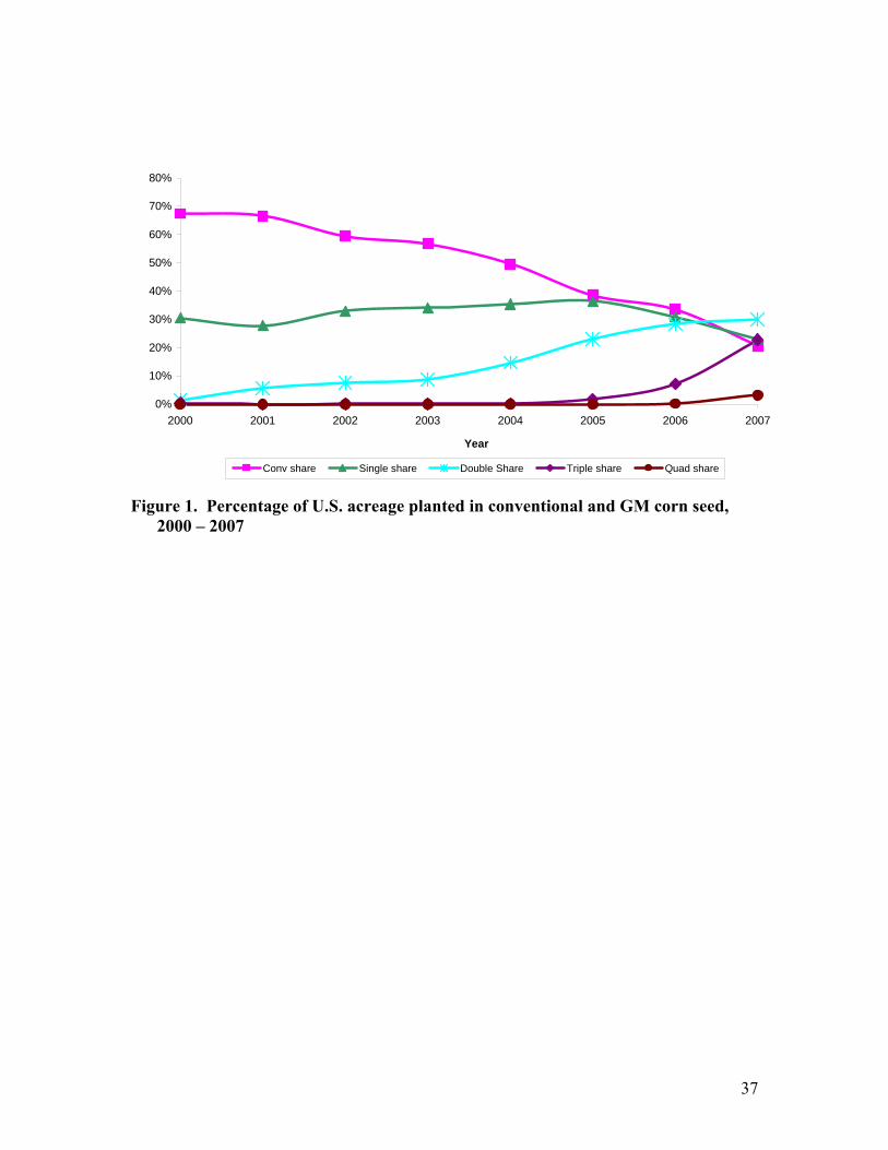
greater flexibility in making spring planting decisions. Figure 1 shows the evolution of
corn acreage shares reflecting adoption rates of conventional and GM hybrid corn seed in
the US from 2000 to 2007 using the dmrk data. The acreage share of conventional seeds
decreased rapidly: from 67.5% in 2000 to 20.6% in 2007. Table 1 presents the average
price of different hybrid corn seeds ($ per bag) in our sample. The presence of a biotech
trait tends to add value to the conventional germplasm and multiple trait-stacking or
bundling is typically worth more than single-trait seeds. Note that, being at the national
level, the information presented in figure 1 and table 1 masks important spatial market
differences. For example, in spite of a rapid adoption of biotech seeds, the dmrk data
show that conventional seeds still dominate in some local markets. This indicates the
presence of spatial heterogeneity in the U.S. corn seed market. As discussed below, such
heterogeneity also applies to seed prices.
9

Econometric Specification
Our analysis of corn seed prices builds on equation (3). As derived, equation (3) is a
structural equation reflecting the determinants of pricing in a multi-product quantity-
setting game.11 As discussed in the model section, cost can affect bundle pricing. Also,
the effects of imperfect competition on price were shown to depend on the nature of
substitution/complementarity across traits. Below, we specify a modified version of
equation (3) that reflects the effects of both bundling and market structure on corn seed
prices.
Consider the case of seeds exhibiting different genetic characteristics. Partition
the set of seeds into mutually exclusive types. Let iK ∈ {0, 1} be a dummy variable for a
seed of the i-th characteristics, i = 1, …, J. In our analysis, we consider J = 5.
Conventional seeds are denoted by 1K = 1, while { 2K , …, 5K } correspond to the GM
traits in corn seeds. The GM seeds include two insect resistance traits: resistance to
European corn borer ECB and to root worm RW 2(K =1) 1)3(K = and two herbicide
tolerance traits HT1 and HT2 4(K =1) 1)5(K = .12 Single-trait GM seeds include only one
GM trait. But bundled/stacked GM seeds include more than one GM trait. We let 1iK = if
a GM seed includes the i-th GM trait (either individually or stacked), and
otherwise. In the absence of bundling/stacking, the K’s satisfy
0iK =
11.J
iiK
==∑ However, in
the presence of stacking, biotech seeds include the genetic traits of more than one type,
implying that Therefore, evaluating the effects of the genetic characteristics
on seed prices requires a flexible specification that can capture bundling/stacking effects.
11.J
iiK
=≥∑
10

We start with a standard model in which each purchase observation is at the farm-
level and the price of a seed varies with its characteristics (e.g., following Rosen 1974).
The price p represents the net seed price paid by farmers (in $ per bag).13 Consider the
hedonic equation representing the determinants of the price p for a seed of characteristics
1 2 5{ , ,..., }:K K K
(5a) 5 5 5 5 5 5 5 5 5 5
1 1 2 1 1 2 1 1 1 2,i i ij ij ijz ijz ijzr ijzr
i j i i z j j i i r z z j j i ip K K K Kβ δ δ δ δ
= = + = = + = + = = + = + = + =
= + + + + + +∑ ∑ ∑ ∑ ∑∑ ∑ ∑ ∑∑ φX ε
where X is a vector of other relevant covariates, and ε is an error term with mean zero
and constant variance. In equation (5a), is a dummy variable for double-stacking the
i-th and j-th GM traits. Similarly, and are dummy variables representing
respectively triple-stacking and quadruple-stacking.
ijK
ijzK ijzrK
14
For conventional seeds and single-trait seeds, the dummy variables and
are all zero. This implies that the coefficients
,ijK ijzK
ijzrK ,ijδ ,ijzδ and ijzrδ in (5a) capture the
supply-side effects of bundling on seed price. The dmrk data reveal that trait bundling is
common, which allows us to test for its price impact. One important special case occurs
when 0ij ijz ijzrδ δ δ= = = , which corresponds to standard component pricing. Here, the
price of seed is just the sum of the value of its genetic components (as captured
by∑ , withi ii Kδ iδ measuring the unit value of the i-th genetic material). When the
parameters ,ijδ ,ijzδ and ijzrδ are not all zero, equation (5a) allows for non-linear pricing
associated with bundled goods under stacking.
11

The parameters ,ijδ ,ijzδ and ijzrδ can be either negative or positive. When
negative, these parameters would reflect sub-additive bundle pricing. The price of the
bundle would then be “discounted” compared to component pricing. This could be
associated with economies of scope on the production side, if the joint production of
bundled goods leads to a cost reduction that gets translated into lower bundle price.
Alternatively, positive parameters would correspond to super-additive bundle pricing.
Next, we introduce market structure effects in (5a) by specifying
(5b) 0 ,i i ii iid d Hδ = +
where, for each CRD, is the traditional HHI in which n nii i in
H∈
≡∑ Ns s n
is represents the
market share of the n-th firm in the market for the i-th characteristics. We construct the
market share using trait acreage. Thus in the GM trait market, only a few biotech firms
owning the patent of each trait are involved. The market share of each company’s trait is
constructed as the firm-specific trait acreage divided by the total trait acreage in the local
market. In the conventional seed market, many more seed companies are involved, and
the market share is constructed as the firm specific conventional seed acreage divided by
total conventional seed acreage in the local market.
We further specify
(5c) , 5 5 5 5
01 1 1 1
ij ij i ji ji jj i i j i i
H K H Kβ β β β= + = = + =
= + +∑ ∑ ∑∑
where n nij ji i j
nH H s
∈
≡ ≡ ∑N
s is the cross-market GHHI that measures concentration for firms
operating in the market for both i-th and j-th characteristics. With this specification, the
coefficients on the GHHI terms capture the net effects associated with efficiency gains,
12

market power, and other possible strategic considerations across different product types.
Since the HHI and the GHHI’s are zero under competitive conditions, it follows from
equations (4) and (5a)-(5c) that the market power component of the price of seed with the
i-th characteristics is given by
(6) 5 5
1 1i ii ii i ij ij i
j i i
M d H K H Kβ= + =
= + ∑ ∑ .
In a way similar to equation (4), equation (6) provides a representation of the
linkages between market structure, imperfect competition, and pricing. As noted in the
model section, the term Mi in (6) measures the difference between price and marginal
cost. It can be used to obtain the associated Lerner index i
i
Mi pL = .
Our model specification allows us to estimate the pricing of each seed type along
with stacking effects. To illustrate, from (5a)-(5c), for a double-stacked seed with ECB
and HT1 , the price equation is 2 4 24( 1, 1, and K K K= = =1)
(7) 5 3
24 0 02 04 24 22 22 44 44 21 21 2 2 4 4 45 453 1
j j i ij i
p d H d H H H H Hβ δ δ δ β β β β= =
= + + + + + + + + + + +∑ ∑ φX ε .
Equation (7) shows how traits, stacking and market concentration are associated
with pricing. Specifically, the 02δ and 04δ terms measure the component value of each
respective trait, 24δ measures the marginal impact of stacking ECB and HT1 in a single
GM seed. The terms capture own-market concentration effects (measured by HHI),
and the β’s capture cross-market concentration effects (measured by the GHHI’s).
iid
The relevant covariates in X include a time trend, each farm’s total corn acreage,
binary terms that control for the source of each transaction, and a set of location
13

variables. The time trend is included to capture advances in hybrid and genetic
technology and other time related factors such as structural changes taking place during
the study years. Farm acreage captures possible price impacts associated with farm size
(including productivity differences and/or volume discounts that could vary with farm
size). Although the surveys defined 16 possible purchasing sources, over 80% of the
transactions were classified into three categories: “Farmer who is a dealer or agent”
(33.1%); “Direct from seed company or their representatives” (29%); and “Myself, I am a
dealer for that company” (16.1%). The source of purchase can capture possible price
differences linked to alternative marketing strategies.
Spatial effects enter our model via state dummy variables along with linear and
quadratic terms for the longitude and latitude of the county. Since the inception of the
hybrid corn seed technology in the 1930s, new hybrids have been developed and
marketed to farms on a regional basis (Griliches 1960). The advent of GM seeds has not
changed the need for seeds to perform well under specific growing conditions that can
vary across regions. Our location variables are designed to control for possible pricing
differences associated with spatial heterogeneity in farming systems (e.g., differing crop
rotations) and agro-climatic conditions (soil quality, length of the growing season,
rainfall patterns, etc.).
The market share of biotech seeds has increased significantly during the years of
our study (see figure 1). In many cases, we found “entry” and “exit” of traited seeds in
some local markets. In order to investigate whether entry/exit may affect seed prices
beyond the H effects, we also introduce entry/exit variables in the specification (5a). In
14

our data, we observe local exits in the conventional seed ( 1K ) markets. We also observe
local entry in the HT1 trait ( 4K ) markets, the ECB trait ( 2K ) markets and the RW trait
( 3K ) markets. To capture entry-exit effects on seed price, the following binary terms are
included: Post-exit1 = 1 for the 1K market; Pre-entry2 = 1 for the 2K market; Pre-entry3
= 1 for the 3K market; and Pre-entry4 = 1 for the 4K market.15
Estimation
Table 2 reports summary statistics of key variables used in the analysis. Each CRD is
presumed to represent the relevant market area for each transaction; thus, all H terms are
calculated at that level. We report the sample mean of the Hii and Hij, across all CRDs for
each seed type. While the average of HHI shows that the conventional seed markets
appear concentrated (with = 0.242, which is above the Department of Justice’s
threshold of 0.18 for identifying "significant market power"), they are not as concentrated
as the biotech trait markets. The average HHI for the three biotech trait markets is over
0.80.
11H
One econometric issue in the specification (5a)-(5c) is the endogeneity of the H’s.
Market concentrations (as measured by the H’s) and seed pricing are expected to be
jointly determined as they both depend on firm strategies. For example, if a major seed
firm uses a strategy focusing on increasing farmers’ adoption, it may price the seed
lower. The low price may increase the firm’s market share and result in higher H’s (for
both HHI and GHHIs). To the extent that parts of the determinants of these strategies are
unobserved by the econometrician, this would imply that the H’s are correlated with the
error term in equation (5a). In such situations, least-squares estimation of (5a)-(5c) would
15

yield biased and inconsistent parameter estimates (due to endogeneity bias). To address
this issue, we first test for possible endogeneity of the H’s using a C statistic calculated as
the difference of two Sargan statistics (Hayashi 2000, p. 232). The test is robust to
violations of the conditional homoscedasticity assumption (Hayashi 2000, p. 232).16 In
our case, the C statistic is 200.16, showing strong statistical evidence against the null
hypothesis of exogeneity of the H’s.
To correct for endogeneity bias, equations (5a)-(5c) are estimated by an
instrumental variable (IV) estimator. We used as instruments the lagged values of each H
and the lagged market size for each seed type. These lagged variables are good
candidates for instruments: given the time lag required to produce seeds, they are part of
the information available to firm managers at the time seed quantity decisions are made.
We investigated the statistical validity of these instruments. The Hansen over-
identification test is not statistically significant, indicating that our instruments appear to
satisfy the required orthogonality conditions. On that basis, equation (5a)-(5c) was
estimated by two-stage-least-square (2SLS).
A second test was used to evaluate the presence of unobserved heterogeneity
across farms. A Pagan-Hall test17 found strong evidence against homoscedasticity of the
error term in (5a). As reported earlier, each farm purchases on average four to five
different seeds. Some large farms actually purchase up to 30 different hybrid seeds in a
single year. Unobserved farm-specific factors affecting seed prices are expected to be
similar within a farm (although they may differ across farms). This suggests that the
variance of the error term in (5a) exhibits heteroscedasticity. On that basis, we relied on
16
heteroscedastic-robust standard errors with clustering at the farm level in estimating
equation (5a)-(5c).
Additional tests of the validity of the instruments were conducted. In the presence
of heteroscedastic errors, we used the Bound et al. (1995) measures and the Shea (1997)
partial 2R statistic to examine the possible presence of weak instruments. The F-statistics
testing for weak instruments were large (i.e., much above 10). Following Staiger and
Stock (1997), this means that there is no statistical evidence that our instruments are
weak. Finally, we conducted the Kleibergen-Paap weak instrument test (Kleibergen and
Paap, 2006).18 The test statistic is 5.81. Using the critical values presented in Stock and
Yogo (2005), this indicated that our analysis does not suffer from weak instruments.
Empirical Results
Equation 5(a)-(5c) is estimated using 2SLS, with heteroscedastic-robust standard errors
under clustering at the farm level. We first tested whether the cross-market GHHI impact
is symmetric: H0: βij = βji, where the β’s are the coefficients of the corresponding
GHHI’s. Using a Wald test, we fail to reject the null hypothesis for . On that basis, we
imposed the symmetry restriction for in the analysis presented below.
13H
13H
Table 3 reports the results. For comparison purpose, the ordinary least square
(OLS) estimation results are also reported. The OLS estimates of the market
concentration parameters differ substantially from the 2SLS results. This reflects the
endogeneity of our market concentration measures (and the associated bias of the OLS
estimation). Our discussion below focuses on the 2SLS estimates. We first discuss the
price impacts associated with introducing single biotech traits. This builds toward a
17

broader assessment of the impacts of bundling/stacking of traits and of the role that
market power. These effects are further investigated below.
Characteristics effects: The coefficients of the terms 2K (ECB), 3K (RW) and 5K
(HT2) show statistically significant price premiums of $25.64, $46.06, and $9.63 per bag,
respectively, over the price of conventional seed. The coefficient of 4K (HT1) is negative
but insignificant.
The coefficients of the terms and provide useful information on the
effects of trait bundling/stacking on seed price. All of the stacking coefficients except for
,ijK ,ijzK ijzrK
35K are negative and statistically significant. The coefficient for 35K is positive but not
statistically significant. As discussed in the econometric specification section, component
pricing is associated with the null hypothesis that all stacking coefficients are zero. Using
a Wald test, the null hypothesis that the stacking coefficients are all zero is strongly
rejected. This provides convincing evidence against component pricing of biotech traits
in the corn seed market. The negative and significant stacking effects also indicate the
potential prevalence of subadditive pricing of corn seed in their individual components.
However, an overall evaluation of the bundling effects also requires including the market
concentration effects. Such an evaluation is presented below.
Market concentration effects: The price effects of changes in the traditional
Herfindahl indexes for each seed type are presented in the first four rows of the “Market
concentration effects” in table 3.19 Our estimates indicate that an increase in market
concentration for conventional seeds (as measured by ) has a positive and statistically
significant association with the price of conventional seeds. More specifically, a one-
11H
18

point increase in is associated with a $14.81 per bag increase in the price of
conventional seeds. The partial effect of concentration in the RW trait market ( ) and
the HT1 trait market ( ), were also positive and statistically significant: A one-point
increase in ( ) is associated with a $32 ($14.92) per bag increase in the price of
RW (HT1) seeds. Finally, the concentration effect in the ECB trait market ( ) is
negative but not statistically significant.
11H
33H
44H
33H 44H
22H
We have argued in the model section that the effects of cross-market
concentration , i ≠ j, depend on the substitutability/complementarity relationship
between traits i and j. We expect that an increase in the cross-market concentration
will be associated with a rise (decrease) in the price if the two components are
substitutes (complements).
ijH
ijH
Of the five GHHI’s that involve conventional seeds ( , , , , ), only
the coefficients on (conventional market share crossed with ECB market share) and
(conventional market share crossed with HT1 market share) are statistically
significant. The positive effect of both coefficients suggests that the ECB trait is viewed
as a substitute for the conventional seed from the perspective of non-GM farmers; and
that conventional seed is viewed as a substitute for the HT1 trait for the HT1 traited seed
adopters. This is plausibly explained by the presence of a “yield drag” associated with
adding a trait into a seed (Avise 2004, p. 41), which would induce some substitution in
demand between GM trait and conventional seed.
12H 21H 13H 14H 41H
12H
41H
19

All the cross-market concentration effects involving biotech traits are statistically
significant. This is a major finding that stresses the importance of the general market
structure in a multi-product setting. The ECB and RW cross-market effects ( and )
are both negative suggesting that insect resistance traits are complements to each other. A
plausible explanation may be that crop damages caused by one insect infestation are
larger in the presence of damages from other insects. The ECB and HT1 effects ( and
) are both positive suggesting that the ECB and HT1 traits are substitutes. The RW
and HT1 effects ( and ) are statistically significant but with opposite sign,
suggesting that the RW trait and HT1 trait may have asymmetric effects on each other:
HT1 trait is viewed as complement to RW trait by RW traited seed adopters; and RW trait
is viewed as substitute for HT1 trait by HT1 traited seed adopters. This suggests that the
effects of insect infestation on corn yield differ significantly from those for weed
infestation.
23H 32H
24H
42H
34H 43H
Location effects: Corn seed prices are found to vary significantly across states.
Compared to Illinois, the price difference is statistically significant for Iowa ($1.53),
Indiana (-$1.13), Ohio (-$2.16), Wisconsin (-$2.34), and Kentucky (-$3.22). It appears
that seed companies are able to price discriminate across regions, reflecting spatial
differences in farmers’ willingness-to-pay, and their demand elasticities. The longitude
variables are not statistically significant. But the latitude variables have significant effects
on corn seed price: the linear term is positive while the quadratic term is negative. Seed
price rises from south to north, reaches a peak near the center of the Corn Belt20 and then
20

declines when moving further north. This confirms significant differences in seed prices
between the center of the Corn Belt and fringe regions.
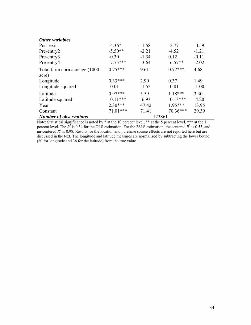
Other variables: Except for Pre-entry4, which represents the entry of HT1 in
specific markets, all other exit and entry dummies are statistically insignificant. The
negative sign on the Pre-entry4 variable indicates that the introduction of HT1 traited
biotech seed may raise the price for all seeds, including the conventional ones. This result
is consistent with the finding in Shi (2009), who argues that the introduction of biotech
seed can raise the conventional seed price. The farm size effect is statistically significant:
large farms within each state pay more for corn seed.21The time trend effect is positive
and statistically significant, possibly capturing the effect of inflation.
Finally, we found statistically significant differences in pricing across seed
purchase sources. Compared to purchasing from “Farmer dealer or agent”, “buying
directly from a seed company” costs about $4.57 less, while purchasing from “myself
dealer” costs about $4.40 less. These results may reflect the effect of farmer’s bargaining
position, but also possibly the presence of price discrimination across different modes of
purchase.
Implications
In this section, our empirical estimates are used to generate additional insights on bundle
pricing, and the interactive role of market structure within and across markets on seed
pricing. Our analysis focuses on Illinois, which is one of the largest corn-producing states
in the US. It has the largest number of farms in our sample. The year 2004 is chosen as it
21

is in the middle of our sample period and it avoids entry/exit events for traits. In each of
our exercises, bootstrapped standard errors are obtained to support hypothesis testing.
Bundling: For the first simulation, we evaluated the effects of bundling/stacking
on seed prices. The bundling literature has identified situations where component pricing
may not apply (e.g., when the demands for different components are correlated, or when
consumers are heterogeneous in at least a subset of the component markets). As discussed
above, an overall evaluation of the bundling effects needs to combine both supply side
and demand side effects. Our econometric results strongly reject component pricing on
the supply side, while finding some statistical evidence that suggests both
complementarity and substitutability in demand (implying the possibility of observing
either sub-additive or super-additive pricing). The simulation results (available upon
request) suggest that, in general, traited seeds generated statistically significant premiums
over conventional seeds, with strong statistical evidence of sub-additive pricing in
bundling two, three, and four traits. Subadditive pricing may be driven by price
discrimination associated with imperfect competition and complementarity in demand, or
the presence of scope economies in the production of bundled/stacked seeds, or both. As
discussed above, scope economies would be consistent with synergies in R&D
investment (treated as fixed cost) across stacked seeds. The subadditivity of prices
encourages more rapid farm adoption of stacked seeds.
Estimated Lerner indexes: Second, we simulate the Lerner indexes applied to the
pricing of different seed types. The Lerner index provides a simple characterization of the
strength of imperfect competition: it is zero under marginal cost pricing, but positive
22

when price exceeds marginal cost. The market power component Mi in equation (6) gives
a measure of price enhancement beyond marginal cost. And the associated Lerner index,
expressed in percentage term, is 100 i
i
Mp× . Evaluated at sample means for Illinois in 2004,
the Lerner indexes are reported in table 4 for selected seed types.
The Lerner indexes are statistically significant at the 5 percent level in four of
eight cases.22 The significant Lerner indexes are positive in three cases: (conventional
seed (5.92%), HT1 traited seed (20.87%), and double stacked seed of ECB and HT1
(15.9%)), and negative in the case of double stacked seed of ECB and RW (-10.11%). The
results provide empirical evidence that market structure affects seed prices. The effect of
market power on price is found to be smallest in the conventional seed market, but large
in the HT1 seed market and the ECB/HT1 bundled seed market. While the Lerner indexes
are not statistically different from zero for single trait ECB and RW seed markets, they
exhibit a negative and statistically significant price effect in the stacked market ECB/RW.
Thus, our analysis shows empirical evidence of complementarities interacting with
market structure: an increased market concentration in these two sub-markets is
associated with a price reduction in the relevant stacked seed market.
Market structure: In our conceptual framework, we develop the GHHI’s
( for sub-markets i and j) as a way to link market structure with pricing in
a multi-product framework. When market shares of different products change, several
GHHIs also change. Thus, the assessment of changing market structures is complex in
the presence of bundling. To evaluate such issues, we simulated the effects of changing
market structures associated with alternative merger scenarios. Several simulations are
n nij i jn
H s∈
≡∑ Ns
23

presented to evaluate the potential effects of increased market concentrations on seed
prices. Each simulation considers a hypothetical merger leading to a monopoly for a
given GM trait market. While these are rather extreme scenarios, the simulated effects
can be interpreted as upper bound estimates of the potential impact of market power.
Three sets of (hypothetical) mergers are simulated: a/ mergers between biotech
companies within each GM trait market (biotech/biotech within trait); b/ mergers
between biotech companies producing different GM traits (biotech/biotech across traits);
and c/ mergers between biotech companies and traditional independent seed companies
(biotech/seed merger). Each merger scenario is counterfactual and used to illustrate how
our analysis can be used to evaluate the price implications of changing market structures.
The price effects of three sets of merger scenarios are reported in table 5. The first
set (scenarios 1-3) considers mergers of biotech firms within the ECB market (scenario
1), within the RW market (scenario 2), and within the HT1 market (scenario 3). As shown
in table 5, the effect of such mergers on seed price would not be statistically significant
for ECB and RW, but would be for HT1. Our simulation results show that mergers of
biotech firms in the HT1 markets could induce a price increase of up to $19.08/bag of
HT1 seed.
The second set (scenarios 4-6) considers mergers between biotech companies
producing different genetic traits. This covers mergers of biotech firms involved in ECB
and RW markets (scenario 4), in ECB and HT1 markets (scenario 5), in RW and HT1
markets (scenario 6). In each case, the simulations assume that the merger leads to a
monopoly in the corresponding market. The cases within scenario 4 allow the evaluation
24

of possible efficiency gains that might emerge from mergers. Mergers across ECB and
RW markets are associated with a price reduction of $5.99/bag for ECB seeds (scenario
4a), $25.10/bag for RW seeds (scenario 4b) and $31.09/bag for ECB/RW stacked seeds
(scenario 4c). Merging ECB and HT1 is shown to have no impact on the ECB trait market
(scenario 5a), but would induce a price increase of up to $22.22/bag for HT1 seed
(scenario 5b) and $22.55/bag for ECB/HT1 stacked seeds (scenario 5c). Merging RW and
HT1 could be associated with a price reduction of up to $21.34/bag for RW seed (scenario
6a) and a price increase of up to $19.91/bag for HT1 seed (scenario 6b). However, the
price effects on RW/HT1 stacked seeds (scenario 6c) are not statistically significant.
Finally, the third set (scenarios 7-9) considers mergers involving biotech
companies and traditional independent seed companies. Again, the simulations assume
that the mergers lead to the monopolization in the corresponding biotech trait market.
However, since the monopolization of seed companies is unlikely (given many seed
companies), the mergers in scenarios 7-9 are assumed to increase market concentrations
for conventional seed only to the maximum observed in our sample. The results show
that the merger involving ECB biotech firms lead to statistically significant price
increases of up to $32.37/bag (scenario 7). The mergers involving RW biotech firms
(scenario 8) or HT1 firms (scenario 9) do not generate statistically significant price
changes. Importantly, these simulation results capture cross-market effects that play a
significant role in the evaluation of the exercise of market power.
The simulations in table 5 illustrate the potential usefulness of the model in
studying the effects of changing market concentrations. For example, in a pre-merger
25
analysis, this would involve evaluating the HHIs and GHHIs in all relevant markets
before and after a proposed merger with a quantitative assessment of the price effects.
Alternatively, the model could be used to estimate the spin-off effects by evaluating the
anticipated effects on HHIs and GHHIs and by simulating the associated price changes.
Concluding Remarks
This paper has presented an analysis of bundle pricing under imperfect competition. A
multiproduct Cournot model identifies the role of substitution/complementarity in bundle
pricing. It explains how oligopoly pricing manifests itself, and motivates generalized HHI
measures of market concentration. The model is applied to the U.S. corn seed market and
is estimated using transaction-level data for the period 2000-2007. The U.S. corn seed
industry is highly concentrated and involves conventionally bred hybrid seeds and other
seeds with various combinations of patented GM traits that add value and service to the
plant. GM seeds compete alongside conventional seeds in a spatially diverse farm sector.
There is considerable variation in the spatial concentration of conventional seeds and
seeds with various patented genetic traits. Through the years analyzed in this study, GM
seeds were adopted quickly among U.S. farmers and are part of a broader wave of
technological progress impacting the agriculture sector.
The econometric investigation documents the determinants of seed prices,
including the effects of bundling and the pricing component associated with imperfect
competition. The research findings yield several major conclusions. . First, we find
extensive evidence of spatial price discrimination. We observe that, ceteris paribus, seed
prices vary by state and in a south to north pricing pattern that peaks in the central part of
26

the Corn Belt. This would be consistent with a type of price discrimination pattern that
reflects the varying productivity of land in the Corn Belt. Second, we find strong
evidence of subadditive bundle pricing, thus rejecting standard component pricing. This
is consistent with the presence of economies of scope in seed production and/or demand
complementarities. Third, we investigated the interactive role of market concentrations
with complementarity/substitution effects in the pricing of seeds. Using generalized
HHI’s, this helps to document how traditional and cross-market effects of imperfect
competition can contribute to higher (or lower) seed prices. For example, our results
indicate that Lerner indices are positive and statistically significant for three seed types.
Fourth, our simulation of hypothetical mergers produced numerous interesting results. It
documented how complementarity effects can contribute to lower prices. It also found
that mergers between a biotech firm and conventional seed firm can contribute to
increasing conventional seed price. Such a price increase may be of concern to
policymakers if it contributed to raising the price of the entire corn seed complex.
Our analysis could be extended in several directions. First, it would be useful to
explore the implications of bundle pricing and imperfect competition in vertical markets.
Second, there is a need for empirical investigations of bundle pricing analyzed jointly
with bundling decisions. Third, it would be useful to investigate farmers’ adoption
behavior with a focus on dynamics and social learning in the presence of bundling and
imperfect competition. Finally, there is a need to explore empirically the economics of
bundling applied to other sectors. These appear to be good topics for further research.
27
References
Adams, W., and J. Yellen. 1976. “Commodity Bundling and the Burden of Monopoly.”
Quarterly Journal of Economics 90:475-498.
Avise, J.C. 2004. The Hope, Hype & Reality of Genetic Engineering: Remarkable Stories
from Agriculture, Industry, Medicine, and the Environment. US: Oxford
University Press.
Baumol, W.J., J.C. Panzar, and R.D. Willig. 1982. Contestable Markets and the Theory
of Industry Structure. New York: Harcourt Brace Jovanovich.
Bound, J., D.A. Jaeger, and R. Baker. 1995. “Problems with Instrumental Variables
Estimation When the Correlation between the Instruments and the Endogenous
Explanatory Variable is Weak.” Journal of the American Statistical Association
55(292):650-659.
Fang, H., and P. Norman. 2006. “To Bundle or Not to Bundle.” Rand Journal of
Economics 37:946-963.
Fernandez-Cornejo, J. 2004. The Seed Industry in U.S. Agriculture: An Exploration of
Data and Information on Crop Seed Markets, Regulation, Industry Structure, and
Research and Development. Washington DC: U.S. Department of Agriculture,
AIB No. 786.
Fulton, M., and K. Giannakas. 2001. “Agricultural Biotechnology and Industry
Structure.” AgBioForum 4(2):137-151.
28

Graff, G., G. Rausser, and A. Small. 2003. “Agricultural Biotechnology’s
Complementary Intellectual Assets.” Review of Economics and Statistics 85:349-
363.
Griliches, Z. 1960. “Hybrid Corn and the Economics of Innovation.” Science 132:275-
280.
Hayashi, F. 2000. Econometrics. Princeton: Princeton University Press.
Hicks, J.R. 1939. Value and Capital: An Inquiry into Some Fundamental Principles of
Economic Theory. Oxford: Clarendon Press.
Hyde, J., M.A. Martin, P. Preckel, and C.R. Edwards. 1999. "The Economics of
Bt Corn: Valuing the Protection from the European Corn Borer." Review
of Agricultural Economics 21:442-454.
Kleibergen, F., and R. Paap. 2006. “Generalized Reduced Rank Tests Using the
Singular Value Decomposition.” Journal of Econometrics 133:97-126.
Kreps, D.M, and J.A. Scheinkman. 1983. “Quantity Precommitment and Bertrand
Competition Yield Cournot Outcomes.” The Bell Journal of Economics
14(2):326-337.
McAfee, R. P., J. McMillan, and M. Whinston. 1989. “Multiproduct Monopoly,
Commodity Bundling, and Correlation of Values.” Quarterly Journal of
Economics 103:371-383.
Pagan, A.R., and D. Hall. 1983. “Diagnostic Tests as Residual Analysis.” Econometric
Reviews 2(2):159-218.
29

Payne, J., J. Fernandez-Cornejo, and S. Daberkow. 2003. "Factors Affecting the
Likelihood of Corn Rootworm Bt Seed Adoption." AgBioForum 6: 79-86.
Rosen, S. 1974. “Hedonic Prices and Implicit Markets: Product Differentiation in Pure
Competition.” Journal of Political Economy 82:34-55.
Shea, J. 1997. “Instrument Relevance in Multivariate Linear Models: A Simple
Measure.” Review of Economics & Statistics 79(2):348-352.
Shi, G. 2009. “Bundling and Licensing of Genes in Agricultural Biotechnology.”
American Journal of Agricultural Economics 91(1):264-274.
Staiger, D., and J.H. Stock. 1997. “Instrumental Variables Regression with Weak
Instruments.” Econometrica 65(3):557-586.
Stock, J.H., and M. Yogo. 2005. “Testing for Weak Instruments in Linear IV
Regression.” In D.W.K. Andrews and J.H. Stock, eds. Identification and
Inference for Econometric Models: Essays in Honor of Thomas Rothenberg. UK:
Cambridge University Press, pp. 80-108.
Venkatesh, R., and W. Kamakura. 2003. “Optimal Bundling and Pricing under a
Monopoly: Contrasting Complements and Substitutes from Independently Valued
Products.” Journal of Business 76(2):211-231.
Whinston, M.D. 2006. Lectures in Antitrust Economics. Cambridge: MIT Press.
30

Table 1. Average Nominal Price for Different Seeds ($ per bag), 2000 - 2007
Year Conv. ECB Single RW Single HT Single Double Triple Quadruple
2000 79.37 100.24 n/a 87.34 95.21 100.95 n/a
2001 80.73 103.77 n/a 89.85 100.43 105.29 n/a
2002 81.81 103.91 n/a 89.08 103.19 94.64 n/a
2003 83.79 104.93 114.88 94.73 108.78 82.10 n/a
2004 86.42 108.61 120.49 98.88 113.68 112.21 n/a
2005 86.96 104.46 114.52 101.50 114.49 123.78 n/a
2006 91.36 109.69 116.67 109.93 123.03 139.21 131.29
2007 93.53 111.36 121.07 114.67 124.71 133.02 140.03
Total 84.29 105.37 117.33 101.51 118.25 133.47 139.60
31

Table 2. Summary Statistics
Variable Number of
observations
Mean Standard
Deviation
Minimum Maximum
Price ($) 139410 99.61 23.61 3 230
Farm size (acre) 30273 489.48 587.87 5 15500
Longitude 30273 91.59 4.783 80.75 103.76
Latitude 30273 41.71 2.010 36.71 46.98
11H 639 0.242 0.152 0.067 1
22H 639 0.769 0.188 0.337 1
33H 313 0.907 0.150 0.430 1
44H 639 0.772 0.175 0.434 1
12H 601 0.085 0.070 0.99E-04 0.518
13H 291 0.108 0.088 1.10E-03 0.632
14H 580 0.075 0.079 9.58E-05 0.526
23H 312 0.761 0.169 0.172 1
24H 617 0.577 0.261 0.010 1
Note: The data contain 139410 observations from CRDs spanning 8 years (2000-2007). Each farm purchases multiple seeds, therefore the number of observations for farm size is the total count of farms per year. The longitude and latitude information is based on the county level measurement for each farm. For the market concentration measurements H’s, we only report the summary statistics of those non zeros at the CRD level, therefore the number of observations is at most 80× 8 = 640.
34H 311 0.785 0.198 0.056 1
32

Table 3. OLS and 2SLS Regression with Robust Standard Errors
OLS 2SLS
Dependant Var: Price ($/bag) Coefficient t-statistics Coefficient Robust z statistics
Characteristic effects, benchmark is K1: Conventional seed 2K (ECB) 24.31*** 46.93 25.64*** 12.65 3K (RW) 31.89*** 23.82 46.06*** 5.09 4K (HT1) 1.93*** 2.97 -3.78 -1.16
5K (HT2) 6.92*** 18.68 9.63*** 10.28 23K -9.49*** -11.20 -11.20*** -7.06 24K -10.06*** -30.10 -13.83*** -13.75 25K -3.44*** -7.96 -5.82*** -6.00 34K -11.03*** -12.74 -14.35*** -10.13 35K 0.39 0.33 -1.27 -0.67 45K -19.70** -2.25 -21.95*** -2.92 234K -24.52*** -28.17 -30.62*** -11.82 235K -13.63*** -12.26 -18.71*** -6.47 245K -16.51*** -24.34 -22.92*** -11.84 345K -12.26*** -6.17 -17.36** -5.98 2345K -28.85*** -24.78 -37.88*** -10.05
Market concentration effects 11H (conventional seed) 11.71*** 15.83 14.81*** 6.47 22H (ECB) 1.45** 2.41 -0.57 -0.27 33H (RW) 4.82** 2.04 32.00*** 2.93 44H (HT1) 11.25*** 12.70 14.92*** 2.91 12H on conventional seed 28.06*** 11.72 36.07*** 3.10
21H on ECB trait -7.22*** -4.73 -7.29 -0.95 13H on conventional seed/RW
trait -1.74 -1.00 2.78 0.21
14H on conventional seed -24.19*** -9.93 -14.58 -1.04
41H on HT1 trait 9.22*** 6.49 22.42* 1.78 23H on ECB trait -2.10*** -6.14 -3.42** -2.38
32H on RW trait 1.79 0.74 -28.87*** -3.45 24H on ECB trait -2.58*** -5.10 3.00* 1.66
42H on HT1 trait 6.53*** 9.59 10.07*** 4.17 34H on RW trait -8.41*** -4.54 -24.98*** -2.98
43H on HT1 trait 3.99*** 9.35 7.77*** 4.15
33
Other variables Post-exit1 -4.36* -1.58 -2.77 -0.59 Pre-entry2 -5.50** -2.21 -4.52 -1.21 Pre-entry3 -0.30 -1.34 0.12 -0.11 Pre-entry4 -7.75*** -3.64 -6.57** -2.02 Total farm corn acreage (1000 acre)
0.75*** 9.61 0.72*** 4.68
Longitude 0.33*** 2.90 0.37 1.49 Longitude squared -0.01 -1.52 -0.01 -1.00 Latitude 0.97*** 5.59 1.18*** 3.30 Latitude squared -0.11*** -6.93 -0.13*** -4.20 Year 2.30*** 47.42 1.95*** 13.95 Constant 71.01*** 71.41 70.36*** 29.39 Number of observations 123861
Note: Statistical significance is noted by * at the 10 percent level, ** at the 5 percent level, *** at the 1 percent level. The R2 is 0.54 for the OLS estimation. For the 2SLS estimation, the centered R2 is 0.53, and un-centered R2 is 0.98. Results for the location and purchase source effects are not reported here but are discussed in the text. The longitude and latitude measures are normalized by subtracting the lower bound (80 for longitude and 36 for the latitude) from the true value.
34

Table 4. Simulated Lerner Indexes
Lerner Index (100 × L) Standard Error t-ratio
Conventional 5.92*** 1.51 3.91
ECB single -2.44 2.05 -1.19
RW single -8.99 6.31 -1.43
HT1 single 20.87*** 2.79 7.47
ECB/RW double -10.11** 5.02 -2.01
ECB/HT1 double 15.90*** 2.89 5.50
RW/HT1 double 8.47 6.72 1.26
ECB/RW/HT1 triple 6.00 5.64 1.06
Note: Lerner indexes are calculated from prices at the mean GHHI levels compared to the case of competition (GHHI=0). Statistical significance is noted by * at the 10 percent level, ** at the 5 percent level, and *** at the 1 percent level.
35
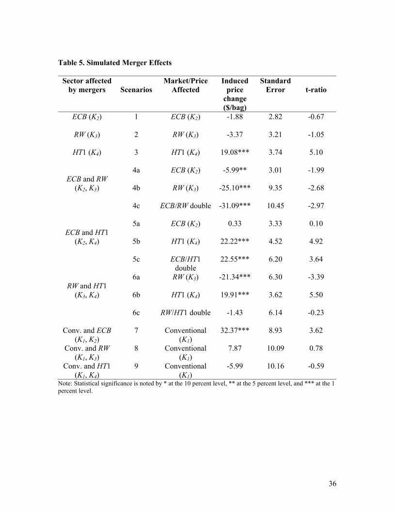
Table 5. Simulated Merger Effects
Sector affected by mergers
Scenarios
Market/Price Affected
Induced price
change ($/bag)
Standard Error
t-ratio
ECB (K2) 1 ECB (K2) -1.88 2.82 -0.67
RW (K3) 2 RW (K3) -3.37 3.21 -1.05
HT1 (K4) 3 HT1 (K4) 19.08*** 3.74 5.10
4a ECB (K2) -5.99** 3.01 -1.99
4b RW (K3) -25.10*** 9.35 -2.68
ECB and RW
(K2, K3)
4c ECB/RW double -31.09*** 10.45 -2.97
5a ECB (K2) 0.33 3.33 0.10
5b HT1 (K4) 22.22*** 4.52 4.92
ECB and HT1
(K2, K4)
5c ECB/HT1 double
22.55*** 6.20 3.64
6a RW (K3) -21.34*** 6.30 -3.39
6b HT1 (K4) 19.91*** 3.62 5.50
RW and HT1
(K3, K4)
6c RW/HT1 double -1.43 6.14 -0.23
Conv. and ECB (K1, K2)
7 Conventional (K1)
32.37*** 8.93 3.62
Conv. and RW (K1, K3)
8 Conventional (K1)
7.87 10.09 0.78
Conv. and HT1 (K1, K4)
9 Conventional (K1)
-5.99 10.16 -0.59
Note: Statistical significance is noted by * at the 10 percent level, ** at the 5 percent level, and *** at the 1 percent level.
36
0%
10%
20%
30%
40%
50%
60%
70%
80%
2000 2001 2002 2003 2004 2005 2006 2007
Year
Conv share Single share Double Share Triple share Quad share
Figure 1. Percentage of U.S. acreage planted in conventional and GM corn seed, 2000 – 2007
37

Footnotes
( )nnF S
mm
1 The CR4 indexes (and the acreage statistics) are calculated from the survey data discussed
below.
2 Single-trait GM corn seeds were first commercialized in 1996. Two years later the double-
stacked corn seed (i.e., the bundling of two traits) was introduced, followed by the introduction
of the triple-stacked system, and then the quadruple-stacked system in 2006.
3 They are: Monsanto, Syngenta, Dow AgroSciences, DuPont, Bayer CropScience, and BASF.
4 Note that, under Cournot behavior, equation (1c) is a necessary but not sufficient condition for
profit maximization by the n-th firm. For example, equation (1c) does not include the role of
fixed cost which affects the non-negative profit condition πn ≥ 0. To the extent that
fixed cost can generate economies of scope (as discussed above), it means that equation (1c)
cannot reveal direct information on economies of scope. However, indirect information about
economies of scope can still be obtained as scope benefits would affect the observed prices and
market share of each firm (through the profit condition πn ≥ 0).
5 As pointed out by an anonymous reviewer, the Lerner index captures information only about the
difference between price and marginal cost. As such, it neglects information about fixed cost
and its effect on firm profit.
6 The markets shares are often expressed in percentage term in the calculation of the Herfindahl-
Hirschman index. Then, the rule becomes H > 1000 (Whinston 2006).
7 The firm dmrkynetec changed its name to GfK Kynetec in May 2009, web address:
www.gfk.com. The seed data set is one of their products, called TraitTrak.
8 The survey is stratified to over-sample large corn producers. The sampling weights are
constructed using farm census data.
38

2 3 1i ij ijz ijzrK K K K
9 They are: IL, IN, IA, KS, KY, MI, MN, MO, NE, OH, SD, and WI.
10 Yield loss due to ECB or RW has been estimated for each to average about 5% with wide
variability over time and space (Hyde et al, 1999; Payne, Fernandez-Cornejo and Daberkow,
2003).
11The use of a quantity setting assumption is motivated in two ways. First, due to time lags in the
production of seeds, the quantity of each seed type is determined in the previous growing year:
seed firms contract with farmers to produce conventional and GM hybrids. Second, price
games under a capacity constraint map to quantity setting outcomes (Kreps and Scheinkman
1983).
12 In our data, we observe that farmers purchase seeds inserted with both herbicide tolerance
traits, implying that farmers see HT1 and HT2 as being differentiated.
13 We also estimated a log specification of the price equation. The econometric results were
qualitatively similar to the ones reported below.
14 Note that the K’s in (5a) satisfy − − − =∑ ∑∑ ∑∑∑ ∑∑∑∑
5 ,
, because
the trait dummy variable K’s are double-counted once in the double stacking dummies, twice in
the triple stacking dummies, and three times in the quadruple stacking dummies. This equality
implies that these dummy variables are perfectly collinear with the intercept. To deal with this
issue below, we set δ1 = 0 in (5a), meaning that the intercept reflects the price of conventional
seeds and that the other δ parameters measure price differences relative to conventional seeds.
15 Note that we do not construct an event dummy for K as we do not observe any pattern of
entry or exit for this trait.
39

15
16 Under conditional homoskedasticity, the C statistic is numerically equivalent to a Hausman test
statistic.
17 Compared to the Breusch-Pagan test, the Pagan-Hall test is a more general test for
heteroscedasticity in an IV regression, which remains valid in the presence of heteroscedasticity
(Pagan and Hall 1983).
18 Note that the Kleibergen-Paap test is a better choice compared to the Cragg-Donald test for
weak instruments: the former remains valid under heteroscedasticity (while the latter one does
not).
19 We do not observe non-zero H because no firm that operates in HT2 market sells a
conventional seed. Similar situations arise for 25 ,H 35H and 45H . Finally, note that 55H = 1
because only one firm operates in this trait market.
20 For the latitude, the peak is reached at 40.54. Note the mean latitude of our study region is
41.71.
21 This suggests that larger farms may be relatively more productive (compared to smaller farms)
and thus may have a higher willingness to pay for seeds. Note that this result is conditional on a
particular purchase source. Note that, as pointed by the Editor, larger farms are also more likely
to be dealers (who tend to face lower prices, as discussed below).
22 Cases involving the HT2 trait are dropped due to lack of variation in the HT2 market
concentration.
40