Embed Size (px)
Citation preview
NPS ARCHIVE1997., 03TSAMILIS, S.
NAVAL POSTGRADUATE SCHOOLMonterey, California
THESIS
ThesisT8227963
NONLINEAR ANALYSIS OF COUPLEDROLL/SWAY/YAW STABILITY
CHARACTERISTICS OF SUBMERSIBLEVEHICLES
by
Sotirios E. Tsamilis
March, 1997
Thesis Advisor: Fotis A. Papoulias
Approved for public release; distribution is unlimited.

OUDLEYKNO/ .tBRARYWVAl ^OSTGftADlJATESCHOOiVIONTERE> :> '3943-5101
DUDLEY KNOX LIBRARY^^^NAVAL POSTGRADUATE
SCHOOL
MONTEREY. CA 93943-5101
REPORT DOCUMENTATION PAGE Form Approved OMB No. 0704-0188
Public reporting burden for this collection of information is estimated to average 1 hour per response, including the time for reviewing instruction, searching existing
data sources, gathering and maintaining the data needed, and completing and reviewing the collection of information. Send comments regarding this burden estimate
or any other aspect of this collection of information, including suggestions for reducing this burden, to Washington Headquarters Services, Directorate for
Information Operations and Reports, 1215 Jefferson Davis Highway, Suite 1204, Arlington, VA 22202-4302, and to the Office of Management and Budget,
Paperwork Reduction Project (0704-0188) Washington DC 20503.
1 . AGENCY USE ONLY (Leave blank) 2. REPORT DATEMarch 1997
3. REPORT TYPE AND DATES COVEREDMaster's Thesis
4 TITLE AND SUBTITLE NONLINEAR ANALYSIS OF COUPLEDROLL/SWAY/YAW STABILITY CHARACTERISTICS OFSUBMERSIBLE VEHICLES
6. AUTHOR(S) Sotirios E. Tsamilis
5. FUNDING NUMBERS
7. PERFORMING ORGANIZATION NAME(S) AND ADDRESS(ES)
Naval Postgraduate School
Monterey CA 93943-5000
PERFORMINGORGANIZATIONREPORT NUMBER
9. SPONSORING/MONITORING AGENCY NAME(S) AND ADDRESS(ES) 10. SPONSORING/MONITORINGAGENCY REPORT NUMBER
11. SUPPLEMENTARY NOTES The views expressed in this thesis are those of the author and do not reflect the
official policy or position of the Department of Defense or the U.S. Government.
12a. DISTRIBUTION/AVAILABILITY STATEMENT
Approved for public release; distribution is unlimited.
12b. DISTRIBUTION CODE
13. ABSTRACT (maximum 200 words)
The problem of coupled roll, sway, and yaw stability analysis of submersible vehicles is analyzed, with
particular emphasis on nonlinear studies. Previous results had indicated that a primary loss of stability is through
the development of limit cycles. This loss of stability is due to the coupling of roll into sway and yaw and cannot
be predicted by considering the uncoupled dynamics. In this study, it is shown that the mechanism of loss of
stability is through bifurcations to periodic solutions. These are characterized as either subcritical or supercritical,
depending on the sign of a certain nonlinear coefficient. Implications of these results to vehicle performance and
operations are discussed.
14. SUBJECT TERMS SHIP STEERING BIFURCATIONS LIMIT CYCLES 15. NUMBER OFPAGES 84
16. PRICE CODE
17. SECURITY CLASSIFI-
CATION OF REPORT
Unclassified
SECURITY CLASSIFI-
CATION OF THIS PAGE
Unclassified
19. SECURITY CLASSIFI-
CATION OF ABSTRACTUnclassified
20. LIMITATION OFABSTRACTUL
NSN 7540-01-280-5500 Standard Form 298 (Rev. 2-89)
Prescribed by ANSI Std. 239-18 298-102

11
Approved for public release; distribution is unlimited.
NONLINEAR ANALYSIS OF COUPLED ROLL/SWAY/YAWSTABILITY CHARACTERISTICS OF SUBMERSIBLE VEHICLES
Sotirios E. fsamilis
Lieutenant, Hellenic Navy
B.S., Hellenic Naval Academy, 1989
Submitted in partial fulfillment
of the requirements for the degree of
MASTER OF SCIENCE IN MECHANICAL ENGINEERING
from the
NAVAL POSTGRADUATE SCHOOLMarch 1997

Iso

MONTEREY, CA 93943-5101 CNTEREV Q* ^3943-5707
ABSTRACT
The problem of coupled roll, sway, and yaw stability analysis of submersible
vehicles is analyzed, with particular emphasis on nonlinear studies. Previous
results had indicated that a primary loss of stability is through the devel-
opment of limit cycles. This loss of stability is due to the coupling of roll
into sway and yaw and cannot be predicted by considering the uncoupled dy-
namics. In this study, it is shown that the mechanism of loss of stability is
through bifurcations to periodic solutions. These are characterized as either
subcritical or supercritical, depending on the sign of a certain nonlinear coeffi-
cient. Implications of these results to vehicle performance and operations are
discussed.

VI
TABLE OF CONTENTS
I. INTRODUCTION 1
A. PROBLEM STATEMENT 1
B. OBJECTIVES AND OUTLINE 2
II. EQUATIONS OF MOTION 5
A. COORDINATE SYSTEM 5
B. GENERAL FORM OF THE EQUATIONS OF MOTION 5
C. SIMPLIFICATIONS 7
D. SIMPLIFIED EQUATIONS OF MOTION 8
III. LINEAR ANALYSIS 9
A. LINEARIZATION 9
B. LOSS OF STABILITY 10
IV. NONLINEAR ANALYSIS 21
A. INTRODUCTION 21
B. THIRD ORDER EXPANSIONS 22
C. COORDINATE TRANSFORMATIONS 29
D. CENTER MANIFOLD EXPANSIONS 30
vii
E. AVERAGING 37
F. LIMIT CYCLE ANALYSIS 45
G. RESULTS AND DISCUSSION 46
V. CONCLUSIONS AND RECOMMENDATIONS 51
APPENDIX 53
LIST OF REFERENCES 73
INITIAL DISTRIBUTION LIST 75
Vlll

I. INTRODUCTION
A. PROBLEM STATEMENT
The dynamic response of a submersible vehicle operating at the extremes
of its operational envelope is becoming increasingly important in order to en-
hance vehicle operations. Traditionally, dynamic stability of motion is studied
using eigenvalue analysis where the equations of motion are linearized around
nominal straight line level flight paths [Arentzen & Mandel (I960)], [Clayton
&; Bishop (1982)], [Feldman (1987)]. Directional stability in the horizontal
plane is normally studied assuming that coupling between sway/yaw and roll
does not exist. Relaxing this approximation can lead to an oscillatory loss of
directional stability [Cunningham (1993)] which cannot be predicted by un-
coupled sway/yaw motions only. This oscillatory loss of stability can generate
limit cycles in the system, as was confirmed numerically in previous studies
[Cunningham (1993)]. In order to gain a better understanding of the mecha-
nism of this type of loss of stability and the stability properties of the resulting
limit cycles, it is necessary to perform a systematic nonlinear analysis which
is precisely the scope of this work.

B. OBJECTIVES AND OUTLINE
In this work we examine the problem of stability of motion with controls
fixed in the horizontal plane, with particular emphasis on the mechanism of
loss of stability of straight line motion. Coupling between sway/yaw and roll
is taken into consideration. This has its origins in both inertial and hydro-
dynamic coupling. We concentrate on an oscillatory loss of stability case,
where one pair of complex conjugate of eigenvalues of the linearized system
matrix crosses the imaginary axis. This loss of stability occurs in the form
of generic bifurcations to periodic solutions [Guckenheimer & Holmes (1983)].
Taylor expansions and center manifold approximations are employed in or-
der to isolate the main nonlinear terms that influence system response after
the initial loss of stability [Hassard Sz Wan (1978)]. Integral averaging is
performed in order to combine the nonlinear terms into a design stability co-
efficient [Chow & Mallet-Paret (1977)]. Special attention is paid to the study
of the quadratic drag terms as they constitute some of the main nonlinear
terms of the equations of motion. The difficulty associated with the nons-
moothness of the absolute value nonlinearities is dealt with by employing the
concept of generalized gradient [Clarke (1983)], a technique which was utilized
in [Papadimitriou (1994)]. This has the advantage of keeping the linear terms
constant, unlike the linear/cubic approximation typically used in ship roll mo-
tion studies [Dalzell (1978)], where the linear damping coefficient is a function
of the assumed amplitude of motion.
Vehicle modeling in this work follows standard notation [Gertler & Hagen
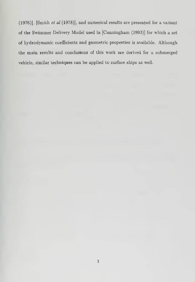
(1976)], [Smith et al (1978)], and numerical results are presented for a variant
of the Swimmer Delivery Model used in [Cunningham (1993)] for which a set
of hydrodynamic coefficients and geometric properties is available. Although
the main results and conclusions of this work are derived for a submerged
vehicle, similar techniques can be applied to surface ships as well.

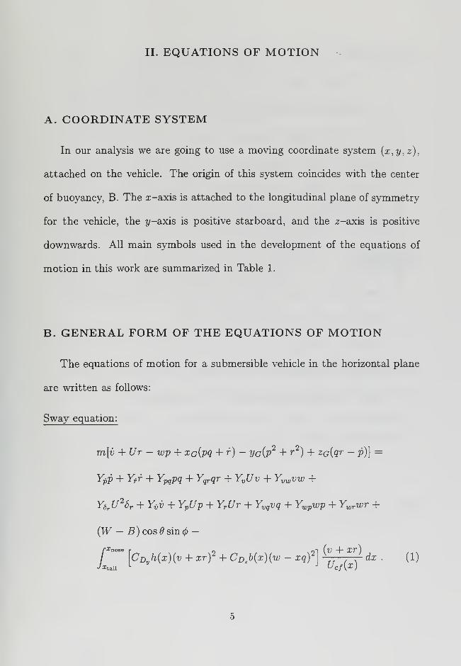
II. EQUATIONS OF MOTION
A. COORDINATE SYSTEM
In our analysis we are going to use a moving coordinate system (x,y,z),
attached on the vehicle. The origin of this system coincides with the center
of buoyancy, B. The rr-axis is attached to the longitudinal plane of symmetry
for the vehicle, the y-axis is positive starboard, and the z-axis is positive
downwards. All main symbols used in the development of the equations of
motion in this work are summarized in Table 1.
B. GENERAL FORM OF THE EQUATIONS OF MOTION
The equations of motion for a submersible vehicle in the horizontal plane
are written as follows:
Sway equation:
m[v + Ur — wp + xc(pq +r) — Vg{p2 + r
2) + zc{qr — p)] =
Ypp + Yri + Ypqpq + Yqrqr + YvUv + Yvwvw +
YsrU26r + YyV + YpUp + YrUr + Yvqvq + Ywpwp + Ywrwr +
(W - B) cos 6 sin 4>-
/\cDy h(x)(v + xr)
2 + CDz b{x){™ ~ xq? -JTTT dx WJxua L J Ucf{x)
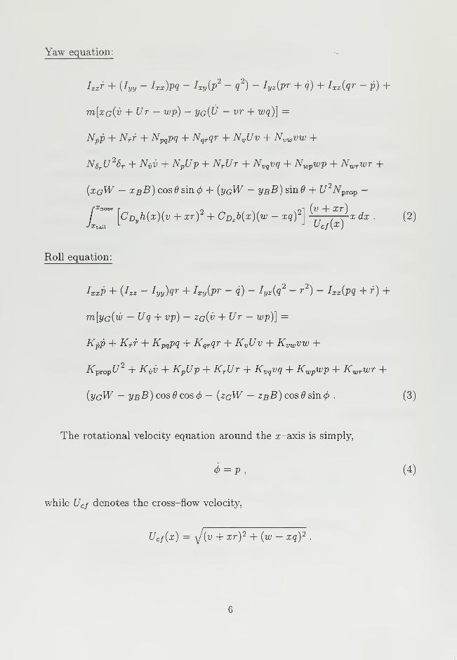
Yaw equation:
IzzT + {Iyy ~ Ixx)PQ ~ Ixy{p2 ~ Q
2)~ Iyz(pr + <j) + IXz(qr ~ p) +
m[xc{v + Ur — wp) - vg{U — vr + wq)} =
Npp + N+r + Npqpq + Nqrqr + NvUv + Nvwvw +
N6rU26r + NyV + NpUp + NrUr + Nvqvq + Nwpwp + Nwrwr +
{xGW - xBB) cos 6 sin <j) + {yGW - yBB) sin0 + U 2NpTOp -
,21 (v + xr
)
/CDy h{x){y + xr)
2 + CDz b{x){w - xq)2
Ucf(x)x dx .
Roll equation:
(2)
IxxP + {hz - Iyy)qr + Ixy (pr - q) - Iyz (q2 - r
2)- Ixz (pq + r) +
m[yo{w — Uq + vp) — zq(v + Ur — wp)] =
Kpp + Kff + Kpgpq + Kqrqr + KvUv + Kvwvw +
-^prop^ + Ki,v + KpUp + KrUr + Kvqvq + Kwpwp + Kwrwr +
{yGW — yBB) cos cos <\> — {zqW — zBB) cos 9 sin<fr
. (3)
The rotational velocity equation around the x-axis is simply,
<t> =P ,
while Ucf denotes the cross-flow velocity,
Ucf(x) = yj{v + xr) 2 + (w - xq) 2.
(4)
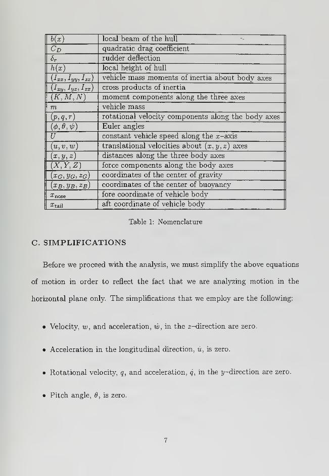
b(x) local beam of the hull
CD quadratic drag coefficient
Sr rudder deflection
h(x) local height of hull
{Lxxi *-yyi * zz) vehicle mass moments of inertia about body axes
\l-xyi *yzi Izx) cross products of inertia
(K,M,N) moment components along the three axes
m vehicle mass
(p,q,r) rotational velocity components along the body axes
(4>,o,1>) Euler angles
u constant vehicle speed along the x-axis
(u,v,w) translational velocities about (x,y, z) axes
{x,y,z) distances along the three body axes
(X,Y,Z) force components along the body axes
{xG,VG,Zg) coordinates of the center of gravity
{xb,Vb,zb) coordinates of the center of buoyancy
•E nose fore coordinate of vehicle body
X tail aft coordinate of vehicle body
Table 1: Nomenclature
C. SIMPLIFICATIONS
Before we proceed with the analysis, we must simplify the above equations
of motion in order to reflect the fact that we are analyzing motion in the
horizontal plane only The simplifications that we employ are the following:
• Velocity, w, and acceleration, w, in the 2-direction are zero.
• Acceleration in the longitudinal direction, it, is zero.
• Rotational velocity, q, and acceleration, q, in the y-direction are zero.
• Pitch angle, 9, is zero.
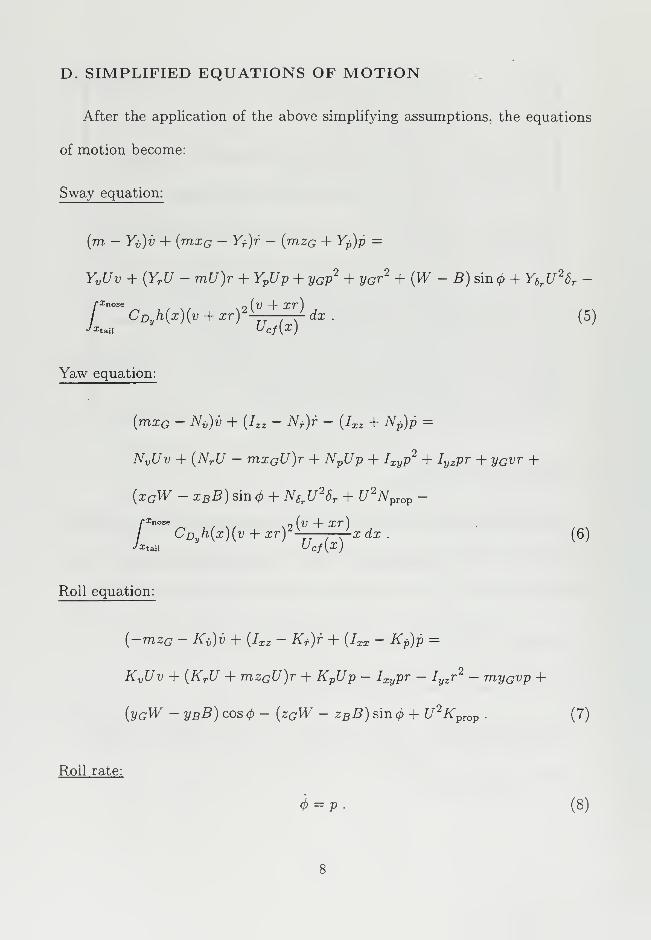
D. SIMPLIFIED EQUATIONS OF MOTION
After the application of the above simplifying assumptions, the equations
of motion become:
Sway equation:
(m - Yy)v + {mxG - Yr)r - (mzG + Yp )p —
2i „._„2 ,
/ T t, D \ • j. , v tt2,YvUv + (YrU - mU)r + YpUp + yGpz + yGr
l + (W - B) sm<j> + Y6rUl6r -
/ CDy h(x)(v + xr)2(—L-J-dx.
(5)
Yaw equation:
{mxG - Nv )v + {Izz - Nr)r - (Ixz + Np )p=
NvUv + (NrU - mxGU)r + NpUp + Ixyp2 + Iyzpr + yGvr +
{xGW - xBB) sin cp + N8rU26T + U 2Nprop
-
/ CDy h(x){v + xr)2
\>x dx . (6)
-/Xtai. Ucf{X)
Roll equation:
{-mzG - Ky)v + {Ixz ~ Kr)-r + (Ixx - Kp)p =
KvUv + (KrU + mzGU)r + KpUp — Ixypr — Iyzr2 — myGvp +
(yGW - yBB)cos4> - {zGW - zBB)sm4> + U 2Kpiop . (7)
Roll rate:
<t>= P- (8)

III. LINEAR ANALYSIS
A. LINEARIZATION
The simplified equations of motion can be written in matrix form as follows:
Ax = Bx + g(x),
where the state vector x is defined as,
x =
V
r
V
and the state matrices are,
A =
m — Yy
mxQ — Nv
-mzQ - Kv
mxG — Yr
hz - N,
J-xz *» r
—vazQ — Yp
-hz - Np
* XX *» p v
1
and
B =
YpUYVU YrU - mUNVU -mxGU + NrU NpUKVU mzGU + KrU KPU10
The term g(x) contains all the nonlinear terms,
9\
92
93
VGP2 + Vgt
2 + (W - B) sin 4> + Y6rU28r -
/"^nose
Coyh(x)(v + xr)\v + xr\ dx
,
IXyP2 + IyzPr + ycvr + (xGW - xBB) sin^ + N6rU
26r
Cd /h(x)(v + xr)\v + xr\x dx
,
(9)
(10)
(11)xtail
O 9= -IxyVT - lyzT ~ myGVp + U ifprop +

{vgW — ijbB) cos 4> — (zGW — zbB) sin
94
(12)
(13)
We want to linearize the nonlinear terms about a nominal point
xo = [vo,r ,po,4>o}T = .
After applying Taylor series expansion of the non-linear terms about the nom-
inal point xo and keeping only the linear components, the linearized equations
of motion are written in matrix form as:
where
and
B' =
Ax = B'x
A' = A,
YVU YrU -mU YPU W - BNVU -mxGU + NrU NPU xGW - xBBKVU mzGU + KrU KPU -zGW + zBB10
(14)
Equation (14) is our linearized system. Eigenvalue analysis for this system is
performed in the next section in order to assess the dynamic stability of the
vehicle.
B. LOSS OF STABILITY
Stability of the linearized system depends on the location of the four eigen-
values of the system, in other words the roots of the characteristic equation:
det{B' - XA') =, (15)
10
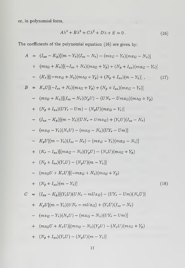
or, in polynomial form,
AX4 + BX 3 + CX 2 + DX + E =.
The coefficients of the polynomial equation (16) are given by:
(16)
A =
+
Ixx - Kp)[{m - YV )(IZZ - Nf ) - (mxG - Yr)(mxG - Nv )}
mzG + Kv )[(-Izz + Nr){mzG + Yp) + (Np + Ixz)(mxG - Yf)]
Kf)[(-mxG + Nv)(mzG + Yp) + (Np + Ixz)(m - Y„)],
B = KvU[(-Izz + Nr){mzG + Yp) + (Np + Ixz)(mxG -Y,)}
mzG + KV )[(IZZ - Nf)(YpU) - (UNr - UmxG){mzG + Yp)
(Np + Ixz)(UYr - Urn) - (NpU)(mxG - Yf)]
Ixx - Kp)[(m - Yv)(UNr - UmxG ) + {YVU){IZZ - N,)
mxG - Yf){NvU) - {mxG - Nv){UYr - Urn)]
- KpU[(m - Yb)(I„ - N,) - (mxG - Y,){mxG - N,)]
+ (K, - Ixz)[(mxG - Ni,)(YpU) - (NvU){mzG + Yp)
[Np + ixz)(yvu) - {Npu)(m - yy]
mzGU + KrU)[(-mxG + Ny)(mzG + Yp )
{Np + Ixz)(m-Yy)}
{Ixx - Kp)[{YvU){UNr - mUxG )- (UYr - Um){NvU)}
+ KpU[{m - Yv){UNr - mUxG ) + {YVU){IZZ - Nf)
mxG - Yf)(NvU) - {mxG - Nv)(UYr - Urn))
(mzGU + KrU)[(mxG - Nv)(YpU) - {NvU){mzG + Yp)
(Np + IXZ){YVU) - (NpU)(m - Yv )}
(17)
(18)
11

+
+
+
+
D =
+
- K
- K
E =
+
(zGW - zBB)[(m - YV ){IZZ - Nr )- {mxG - Yr)(mxG - Nv )]
{mzG 4- Ky)\{xBB - xGW)(mxG - Y,) - (U
N
r - UmxG){YpU)
(UYr - Um)(NpU)}
KV U[(IZZ - Nr){YpU) - {UNr - UmxG){mzG + Yp )
(Np + Ixz){UYr - Um) - (NpU){mxG - Yr )}
(K, - Ixz )[(xBB - xGW){m - Yi)
(NVU)(YPU) + (NPU)(YVU)) , (19)
(mzGU + KrU)[(xBB - xGW)(m - Yy)
(NvU){YpU) + {NpU){Yv U)}
{K,-Ixz )(xBB-xGW)(YvU)
(mzG + Kv ){xBB - xGW){UYr - Um)
vU[(xBB - xGW)(mxG -Yr)
(UNr - mUxG)(YpU) + {UYr - Um)(NpU)}
pU[{YvU){UNr - mUxG )- (UYr - Um)(NvU)}
(zGW - zBB)[(m - Yv)(UNr - mUxG ) + (YVU)(IZZ - Nr )
(mxG - Yr){NvU) - {mxG - Nv){UYr - Um)], (20)
(zGW - zBB)[{YvU){UNr - mUxG )- (UYr - Um)(NvU)}
(KvU){xBB - xGW){UYr - Um)
{mzGU + KrU){xBB - xGW){YvU) (21)
We can examine the stability of the system by utilizing Routh's criterion.
Application of this criterion to the characteristic equation (16), reveals that
12

the following two conditions must be satisfied in order to ensure that all roots
of (16) have negative real parts:
BCD - AD 2 - EB 2 > , (22)
E > . (23)
If E is less than zero, one real root of (16) becomes positive and the sytem will
become unstable in a divergent manner (Guckenheimer and Holmes, 1983).
This is the case of a directionally unstable ship which is well known in the
literature (Clayton and Bishop, 1982). If, however, condition (22) is violated,
the system will exhibit an oscillatory motion due to the presence of complex
conjugate roots with positive real parts. This form of instability is caused by
the coupling of roll into sway and yaw and is further analyzed in this work.
In order to compute the limiting case of loss of stability, we consider equa-
tion (24),
BCD - AD 2 - EB 2 = . (24)
The result of this equation will produce the limiting value of zq as a function
of xq for loss of stability A curve of this functional form,
zg = f(xG ) ,
will be our locus of loss of stability. After some algebra, we can express the
coefficients of equation (24) in the following form:
A = Aiz% + A 2 zG + A 3 , (25)
13
where
A x= -m 2
{Izz -N,)
A 2 = -mYp {Izz - Nf) - mKv (Izz - Nf) + m(Np + Ixz)(mxG - Yf)
+ m(Kr - Ixz){'rnxG - Ny)
A 3 = (Ixx -Kp)(m -YV ){IZZ - N+) - {Ixx - Kp){mxG - Yf){mxG - Nv )
- KVYP {IZZ - Nf) + Kv{Np + Ixz)(mxG - Y+)
+ Yp{Kr - Ixz)(mxG - Ny) - {Kf - IXZ)(NP + Ixz ){m - Yv )
B = B x z2G + B2 zG + B3 , (26)
where
B1= m 2(UNr - UmxG ) + m 2U{mxG - Nv )
B2 = -m(KvU){Izz -Nr)-m{Izz -Nr){YpU)
+ mYp(UNr - UmxG ) + mKv(UNr - UmxG )
- m(Np + Ixz)(UYr - Um) + m(NpU){mxG - Y+)
- m{Kr - IXZ){NVU) + mUYp{mxG - Nv )
- mU(Np + Ixz){m - Yv ) +mUKr(mxG - Nv )
B3 = -Yp(KvU)(Izz -Nr) + {KvU)(Np + Ixz)(mxG -Y,)
- Kv {Izz -N,)(YpU) + KvYp(UNr -UmxG )
- Kv{Np + Ixz){UYr - Um) + Kv {NpU){mxG - Yf )
- {Ixx ~ Kp){m - Yv){UNr - UmxG )- (Ixx - Kp){YvU){Izz - Nf)
+ (Ixx ~ Kp){mxG - Yf)(NvU) + {Ixx - Kp){mxG - Nv)(UYr - Um)
14

- (KpU)(m - Y,){IZZ - Nf) + (KpU)(mxG - Y+)(mx - JV6 )
+ {K, - Ixz)(mxG - Ni,){YpU) - Yp(K, - IXZ )(NVU)
+ (Np + Ixz)(YvU)(Kr - I„) - (K, - Ixz)(NpU)(m - Y,)
+ UKrYp(mxG - N„)
C = Ci4 + C2zG + C3 , (27)
where
d = -m 2U(NvU)
C2 = mU(mxG - Ny)(YpU) - mUYp(NvU) - mUKr(NvU)
+ mUiNp + I^iY^-mUiNpU^m-Yy)
+ W(m- Yt)(I„ - NT )- W{mxG - Yr){mxG - N*)
- m{XBB - xGW)(mxG - Y+) + m{UNr - UmxG){YpU)
- m(UYr - Um){NpU) + m{KvU)(UNr - UmxG )
C3 = (Ixx -Kp){YvU)(UNr -UmxG)-(Ixx -Kp)(UYr -Um){NvU)
+ (KpU)(m - Yi){UNr - UmxG ) + (KPU){YVU){IZZ - N+)
+ (KpU)(mxG - Yr)(NvU) - (KpU)(mxG - Ni)(UYr - Um)
+ UKrimxG-N^YpUj-UKrYpiNvU)
+ UKr(Np + IXZ){YVU) - UKr(NpU)(m - y«)
- Ky(XBB - xGW){mxG - Yr ) + Ky(UNr - UmxG){YpU)
- Ky{UYr - Um){NpU) - {KVU){IZZ - Nr){YpU)
+ Yp(KvU){UNr- UmxG )
- {KVU){NP + Ixz)(UYr - Um)
+ (KvU){NpU){mxG - Yr) + (K* - Ixz){XBB - xGW){m - Y*)
15
- (Kr - IXZ)(NVU)(YPU) + {Kf - IXZ)(NPU)(YVU)
D = D x zG + D 2 , (28)
where
£>i = mU(xBB -xcW^m-Y^-mUiNy^iYpU)
+ mU{NpU){YvU) + m(xBB .- xGW){UYr - Urn)
- W(m - Yy){UNr - UmxG )- W(YVU)(IZ2 - N+)
+ W(mxG -Yr){NvU) + W(mxG - Ny)(UYr - Um)
D 2= UKr (xBB-xGW){m-Yi}
)-UKr(NvU){YpU)
+ UKr(NpU){YvU) - {Kr - Ixz){xBB - xGW){YvU)
+ Ky{xBB - xGW){UYr - Um) - (KvU)(xBB - xGW){mxG - Yr)
+ {KvU)(UNr - UmxG){YpU) - (KvU){UYr - Um){NpU)
- (KpU)(YvU)(UNr - UmxG ) + [KpU)(UKr - Um)(NvU)
and
E = E x zG + E2 , (29)
where
Ei = W{YvU){UNr -UmxG)-W{UYr -Um)(NvU)
- mU{xBB -xGW)(YvU)
E2 = {KvU){xBB -xGW){UYr -Um)-UKr (xBB -xGW)(YvU)
If we apply the stability criterion (24) utilizing expressions (25) through
(29), we get a fifth order polynomial equation in the metacentric height zG of
16
0.065
0.06 -
0.055 -
0.05 -
0.045
' 0.04
0.035
0.03-
0.025 -
0.02 -
0.0150.2 0.4 0.6 0.8 1 1.2 1.4 1.6 1.8
XG (ft)
Figure 1: Critical value of zq versus xq for U — 5 ft/sec
0.07
0.06
0.05
0.04 -
C3M0.03
0.02 -
0.01 -
1 1 1 1 1 1 1
-\ \ .^J^^—-
:23.5
—-+-5
6.5
8
1 1 1I
1 . 1 |
0.2 0.4 0.6 0.8 1
XG1.2 1.4 1.6 1.8
Figure 2: Critical value of zq versus xq for different values of U (ft/sec)
L7

the following form,
F5zG + F4 zG + F3z3
G + F2z% + Fx zG + F =, (30)
where,
»2
Fo = B3C3D 2 — A 3D 2— E2B3 ,
Fi = BzCzD l + (BZC2 + B2C3)D2 - 2E2B2B3 - EXB\
2D2D lA 3 - D\A2 ,
F2 = -E2{Bl + 2B lBz)-2E lB2Bz + {BzC2 + B2Cz)D 1 +
(B3C1 + B2C2 + B lCz)D 2 - D\A 3 - 2D2D 1A 2 - D^ ,
F3 = -D 2
1A 2 -2D2D 1A l -2E2B lB2 -E1 (B% + 2B 1B3 ) +
D^Bzd + B2C2 + B1C3) + D 2 {B2d + BiC2) ,
FA = D 1 {B2Cl + B lC2 ) + B 1ClD 2 -D 21A l -E2B*-2ElB lB2 ,
F5 = -EXB\ + B lClD l .
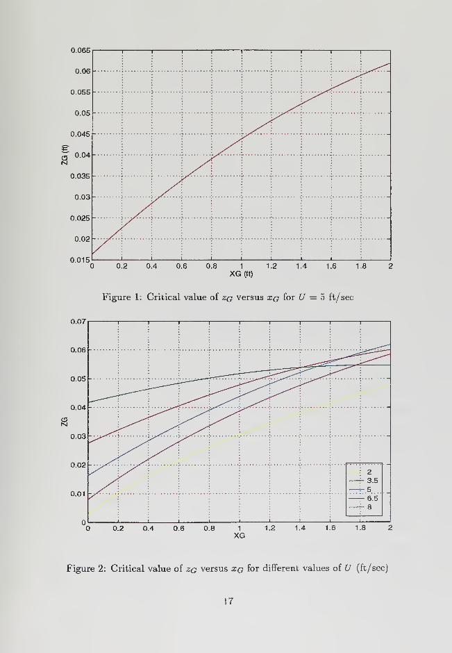
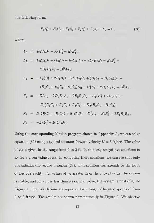
Using the corresponding Matlab program shown in Appendix A, we can solve
equation (30) using a typical constant forward velocity U — 5 ft/sec. The value
of xG is given in the range from to 2 ft. In this way we get five solutions in
zq for a given value of xG . Investigating these solutions, we can see that only
one satisfies the second criterion (23). This solution corresponds to the locus
of loss of stability. For values of zG greater than the critical value, the system
is stable, and for values less than its critical value, the system is unstable, see
Figure 1. The calculations are repeated for a range of forward speeds U from
2 to 8 ft/sec. The results are shown parametrically in Figure 2. We observe
18


an upwards movement of the curves as the speed is increased. This means
that the system experiences a tendency to become less stable at higher speeds
which, in turn, calls for higher metacentric heights to ensure stability.
19

20

IV. NONLINEAR ANALYSIS
A. INTRODUCTION
From the linearized analysis on the loss of stability that was done in the
previous chapter, we can see that as a specific parameter of the system, such as
(xg, zq), is varied, it is possible to pass from a region of stability to a region of
instability. This case of loss of stability is associated with one pair of complex
conjugate eigenvalues of the system crossing the imaginary axis. This loss of
stability is usually accompanied by self sustained oscillations, and it is called
Hopf Bifurcation.
There are two cases of Hopf Bifurcations, supercritical and subcritical. In
the supercritical case, limit cycles are created just after the loss of stability.
A limit cycle is a constant amplitude oscillatory motion of our system. This
amplitude is usually larger as we move away from the bifurcation point. When
the limit cycles have small amplitudes the situation is not very critical for our
vehicle and is not much different from stable conditions. In the subcritical
case we may have convergence to limit cycles, even before our system looses
its stability. Furthermore, the limit cycle amplitudes are considerably higher.
The analysis that will follow will be performed in order to verify the exis-
tence of the limit cycles and to find out which case of Hopf Bifurcations we
have in our model. We will also examine the stability of the resulting limit
cycles. This analysis is necessary because we can predict the behavior of a
21

vehicle when some of its parameters change and we have operation in the
proximity of a bifurcation point. The results of the non linear analysis will
be verified by a numerical simulation of the system's motion, both above and
below the bifurcation point.
B. THIRD ORDER EXPANSIONS
From the linearization procedure we see that our system is written in the
form of matrix equation (14), where we have ignored the non linear terms.
If we take into account the non linear terms up to third order, equation (14)
becomes:
A'x = B'x + g(x), (31)
where,
g(x)
9i{x)
92{x)
9z{x)
94{x)_
Keeping terms up to third order the vector of non linear terms can be written:
g(x)=gW(x)+gW(x) + c(x), (32)
where g^2\x) contains the second order non linear terms, g^\x) contains the
third order non linear terms, and c(x) contains the constant terms. The cross
flow integrals can be written as follows:
Iv =
Ir =xtail
r^nose
Cdv I h(x)(v + xr)\v + xr\ dx"^tail
Panose
Coy / h(x)(v + xr)\v + xr\x dx
22
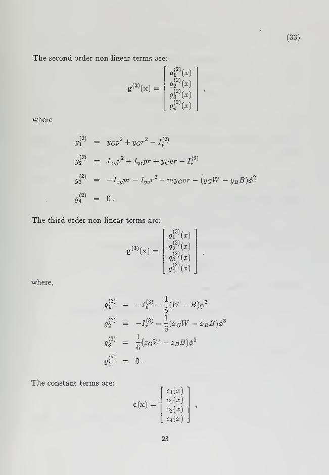
The second order non linear terms are:
r(2)
where
gw (x) =
9?\x)
(33)
(2) _9i
92
93
a{2)
9a
vgp2 + ycr
1 - 42)
= IxyP + IyzPr + VGVT - I.(2)
-Ixypr - Iyzr2 - myGvr - (yGW - yB B)<j)
2
0.
The third order non linear terms are:
(3)f^ -
where,
9i(3)
(3)
92
9?
9?
g,J'(x) =
gi%)9?\*)
= -1^ -\(W - B)4?
= -/<3) - -(xaW - xBB)4?
-{zGW - zB B)<t?
= 0.
The constant terms are:
c(x) =
ci(x)
C2{x)
c4 (x)
23

where,
Cl (x) = YSrU28
2i,r
C2 {X) = N6rU2tr + U 2
Npr0p
c3 (x) = U 2Kpr0p + yGW - yBB
Ci(x) = .
In order to get the second and third order non linear terms of the cross flow-
integrals, we must expand in Taylor series a function of the form:
' no = m\ (34)
about a nominal point £o :
eKI = Col^ol + 2]£o|« - £o) + sign(£ )(£ - Co)2 + /
(3)(£) • (35)
The sign function in equation (33) can be approximated by:
sign(£ ) = limtanh(— ) , (36)y—+0 'V
where the approximation gets better as 7 gets smaller.
If we choose £0 = as our nominal point, equation (35) becomes:
m =^3(37)
07
In our case £ is (v + xr) so we have:
(v + xr)\v + xr\ = — (v + xr) (38)67
or
(v + xr)\v + xr\ = —(v 3 + x3r3 + 3z;
3xr + 3x 2r2t;) (39)
67
24

Using equation (39) the cross flow integrals become:
Iv = -^(E v3 + 3E lv
2r + 3E2vr
2 + E3r3)
67
h =CDy
67(E^ 3 + 3E2v
2r + 3E3vr
2 + EAr3)
where,
xih{x)dx ,i = 0,1,2,3,4
(40)
(41)
(42)^tail
By using this approximation we see that the expansion of the cross flow inte-
grals give only third order terms, so we have:
/,?) = /<*> = (43)
Now we want to write our matrix equation in state space form, so we have to
find the inverse of the system matrix:
(A')/\-l
£11 £12. £12. f)
D D D V
£21 £22. a23 f)
D D D U£21 £22. a33D D D v
1
where,
an
a 13
Q-21
«22
^23
^31
(Izz - N,){IXX - Kp) - (Ixz - K,){-Ixz - Np )
(Yf - mxG )(Ixx ~ Kp) + (Ixz - Kf){-mzG - Yp)
(mxG - Yf){-Ixz - Np) - {Izz - Nr)(-mzG - Yp)
-K - NV )(IXX - Kp) + {-mzG - Ky){-Ixz - Np)
(m - YV )(IXX - Kp) - (-mzG - Kv)(-mzG - Yp)
-(m - Yv)(-Ixz - Np) + (mxG - Nv){-mzG - Yp)
(mxG - NV ){IXZ - Kr) - (-mzG - KV )(IZZ - N+)
25
and
az2 = -(m-Yi,)(Ixz - Kr) + (-mzG- Ki,)(mxG-Yr)
^33 = (m -Yy)(Izz - Nf) - {mxG - Ny)(mxG -Yr)
D = (m-Yv )(Izz -N,)(Ixx -Kp)
- (m - Yi)(Ixz - Kf)(-IXz - Np)
- (mxG - Ny)(mxG - Yr){Ixx - Kp )
+ (mxG - Ny)(Ixz - Kf){-mzG - Yp )
+ (-mzG - Kv)(mxG - Yr){-Ixz - Np)
- (-mzG - Ky)(Izz - Nr)(-mzG -Yp )
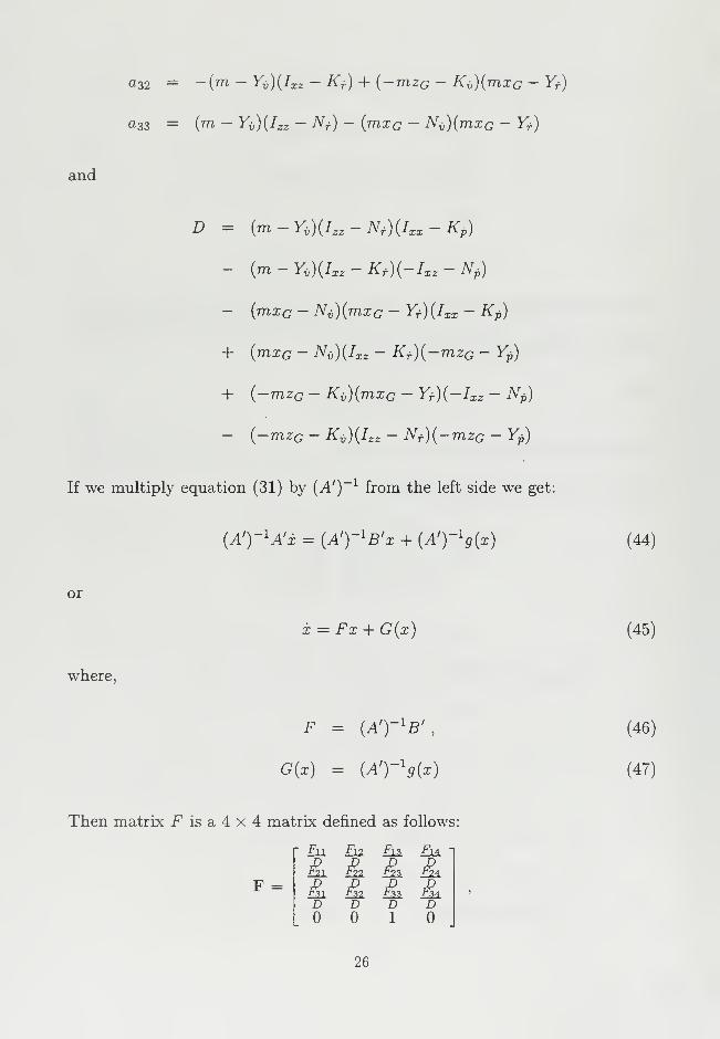
If we multiply equation (31) by (A') from the left side we get
'\-l id' \i\-i{A')-
lA'x = {A'Y'B'x + (A')-l9(x) (44)
or
where,
x = Fx + G(x)
F = {A')-lB'
,
G(x) = {A')-lg{x)
Then matrix F is a 4 x 4 matrix defined as follows:
F =
- F±l Fj2_ Fjji Ft 4
T2I F22 -P23 -T24
Fd F32 .F33 F34D D D D10
(45)
(46)
(47)
26
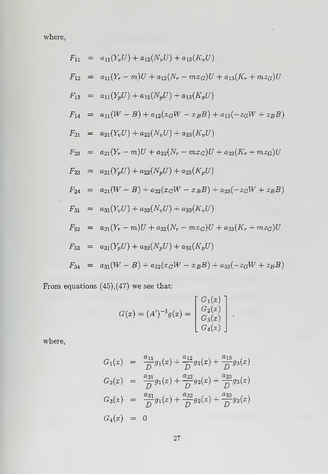
where,
Fu = an (YvU) + a 12{NvU) + a 13(KvU)
F\2 = a>n{Yr - Tn)U + ai2(Nr - mxc)U + ai3(Kr + mza)U
F13= au (YpU) + a l2{NpU) + a 13(KpU)
Fu = au {W -B)+au (xGW - xBB) + a l3 {-zGW + zBB)
F21 = a2l {YvU) + a22(NvU) + a23(KvU)
F22 = a2i(Yr - m)U + a22(Nr - mxG)U + a23(Kr + mzG)U
F23 = a2l {YpU) + a22(NpU) + a23(KpU)
F24 = a2l (W - B) + a22 (xGW - xBB) + a 23 {-zGW + zBB)
F31 = a3l {YvU) + a32(NvU) + a33(KvU)
F32 = a3i(Yr - m)U + a32(Nr - mxG)U + a33(Kr + mzG)U
F33 = a3l (YpU) + a32 {NpU) + a33(KpU)
F34 = a3l (W - B) + a32 (xGW - xBB) + a33(-zGW + zBB)
From equations (45), (47) we see that:
G{x) = (A')-l9(x) =
C?i(«)
G2 (x)
G3 (x)
G4(x) J
where,
n t \fll1
( \ ,
ai2/ \ ,
fll3< \Gi(x) = —9i{x) +—g2 {x) + —g3 {x)
^ t \fl21 < \ ,
a22 / n,
a23 / v
G2 {x) = —gi{x) + —g2 (x) + —g3 {x)
n t \a31 / \ ,
a32 / x,
a33 , s
G3 {x) = —gi{x) + —g2 {x) + —g3 (x)
G4 {x) =
27

Equation (45) can also be written in the following way:
x = Fx + G {2\x) + G (3) (x) + k (48)
where,
and
G^(x) =
G™(x) =
G<2)
(or)
G<2 >(x)
a? (x)
G<2 >
(x)
G<3>(x)
G<3> (x)
G<3> (x)
G<3 >
(x)
fcl
Each element of the above non linear terms vectors can be written as follows:
G?\x)
Gf(x)
fpF>(«) + ^42)M +^2)M
=
and
GfM
G<3,(x)
«31 (3)/ v,
a 32 (3)/ v .
a33 (3)/ v
-fi-9i(*) +—92
J(x) + —9z }
{x)
28

Finally, the constant terms are:
h = TC1 +~D
C2 +~D
C3
a2\ a22 ,
a23k2 =
-dCi +
-dC2 +
-dCz
, &31, ^32
,^33
fc4 = 0.
C. COORDINATE TRANSFORMATIONS
From equations (45) and (48) it is obvious that the stability of our system
depends on the eigenvalues of matrix F. Since we want to investigate the
behavior of our system oround the Hopf Bifurcation point, it is useful to bring
our system in its normal coordinate form. This can be done by applying a
transformation of the coordinate system, using as transformation matrix T,
the modal matrix of eigenvectors of F, evaluated at a critical point. This
critical point will be a pair of zq and xq values, that belong to the critical line
of loss of stability. The applied transformation will be as follows:
x = Tz (49)
or,
z = T~ lx (50)
Then equation (48) can be written as follows:
Tz = FTz + G {2) {Tz) + G {3\Tz) + k (51)
29
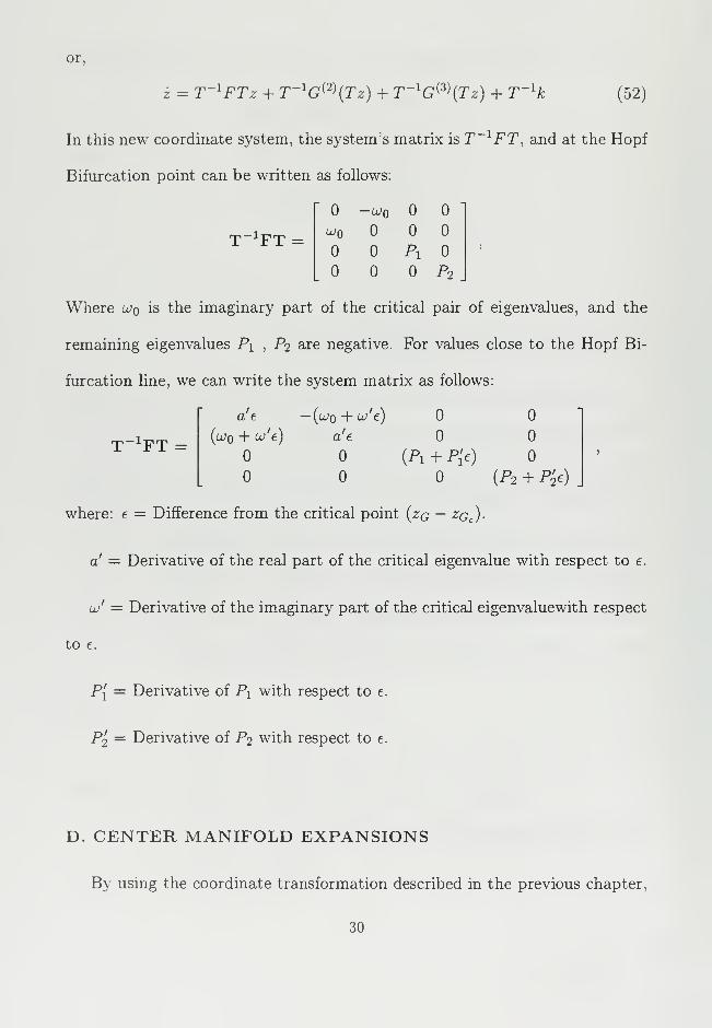
or,
i = T~ lFTz + T- lG {2) {Tz) + T- lG {z){Tz) + T~ l
k (52)
In this new coordinate system, the system's matrix is T 1FT, and at the Hopf
Bifurcation point can be written as follows:
T _iFT =
-wtoo
Pi
P2
Where ujq is the imaginary part of the critical pair of eigenvalues, and the
remaining eigenvalues Pi , P2 are negative. For values close to the Hopf Bi-
furcation line, we can write the system matrix as follows:
T -iFT _
a'e -{uQ + u'e)
(u + w'e) a'e
(Pi + P{e)
{P2 + P&
where: e = Difference from the critical point [zq — zqc )-
a' — Derivative of the real part of the critical eigenvalue with respect to e.
u' = Derivative of the imaginary part of the critical eigenvaluewith respect
tO €.
P[ = Derivative of Pi with respect to e.
P'2 = Derivative of P2 with respect to e.
D. CENTER MANIFOLD EXPANSIONS
By using the coordinate transformation described in the previous chapter,
30
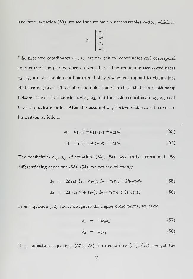
z —
and from equation (50), we see that we have a new variables vector, which is:
z\
Z2
zz
24
The first two coordinates z\ , 22, are the critical coordinates and correspond
to a pair of complex conjugate eigenvalues. The remaining two coordinates
23, 24, are the stable coordinates and they always correspond to eigenvalues
that are negative. The center manifold theory predicts that the relationship
between the critical coordinates z\, 22, and the stable coordinates 23, 24, is at
least of quadratic order. After this assumption, the two stable coordinates can
be written as follows:
23 = hU zj + hyiZ\Z2 + h,22z\ (53)
24 = SU zj + S 122i22 + S 22^| (54)
The coefficients hij, Sy, of equations (53), (54), need to be determined. By
differentiating equations (53), (54), we get the following:
23 = 2h\\Z\Z\ + hu(ziZ2 + 2122) + 2h 22Z2Z2 (55)
24 = 2sn 2 1 2i + Syi{z\Z2 + 2i22 ) + 2522^22 (56)
From equation (52) and if we ignore the higher order terms, we take:
z\ = -wo22 (57)
22 = OOqZi (58)
If we substitute equations (57), (58), into equations (55), (56), we get the
31
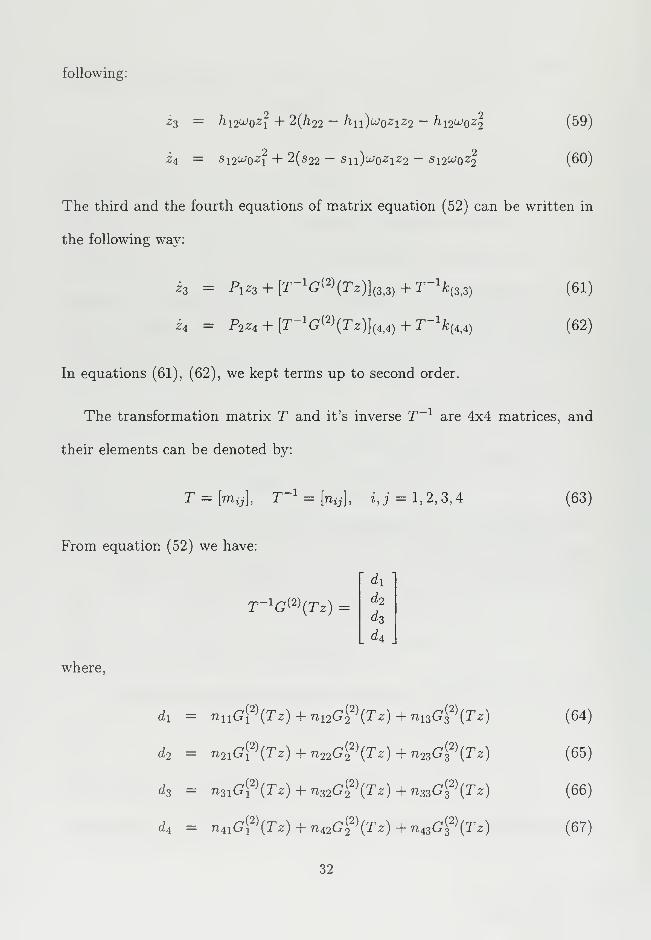
following:
i3 = hi2u) z2 + 2(/i22 - hii)uoziz2 - ^-12^0^2 (
59)
i4 = Si 2U)qz\ + 2(s 22 - Su)u)oZiZ2 - S^O-^ (60)
The third and the fourth equations of matrix equation (52) can be written in
the following way:
h = Piz^ + lT-'G^iTz^^+T-'k^
za = P2Z4 + [T-lG {2\Tz)} (4A) +T-
lk {4A)
In equations (61), (62), we kept terms up to second order.
(61)
(62)
The transformation matrix T and it's inverse T 1are 4x4 matrices, and
their elements can be denoted by:
T = [rriij], T = [n#], i,j = 1,2,3,4 (63)
From equation (52) we have:
T- lG {2) {Tz) =
di
d2
d3
d4
where,
di
d2
d3
d4
nuG {2)(Tz) + n 12G {
22){Tz) + n l3Gf{Tz)
n21G {2)(Tz) + n22G {
22](Tz) + n23G {^(Tz)
n3lG(2)
(Tz) + n 32G {2)(Tz) + n33Gf(Tz)
n4lG {2)(Tz) + n42G {
22)(Tz) + n43G 3
2)(Tz)
(64)
(65)
(66)
(67)
32

Also from coordinate transformation, the relationship between the old and
new coordinates is as follows:
V — m\\Zi + 777,1222 + 777l323 + 777i424 (68)
T = 777,212:1 + 77722^2 + 7772323 + 777-2424 (69)
P = 7773i2i + 7773222 + 7773323 + 7773424 (70)
<p = 7774121 + 777,4222 + 7774323 + 7774424 (71)
Finally if we substitute equations (68), (69), (70), (71), and the expressions for
d, (?2, G3 , G4 into equations (64), (65), (66), (67), we get the final expressions
for the coefficients df
d\ = nn (l 15 zl + l 16z1 z2 + Inzl)
+ n 12 {h5Zi + I26Z1Z2 + I27Z2)
+ n 13 (l35zj + I36Z1Z2 + Z3722) (72)
d<2 = n2i{li5zj + h%z x z2 + Inzl)
+ ^22(^252? + ^262l22 + Z2722)
+ ^23(^352? + ^362l22 + I37Z2) (73)
dz = n3i(l15zl + /i62i22 + Inzfj
+ n32 (l25Zi + I26Z1Z2 + I27Z2)
+ n33 (l35zj + l36Z 1 z2 + Iwzl) (74)
d4 = Tl4i(/i5Z1 + I16Z1Z2 + £l722 )
+ ^42(^252i + ^26^122 + ^2722)
+ 7743(^3521 + /36^i22 + l 37z\) (75)
33
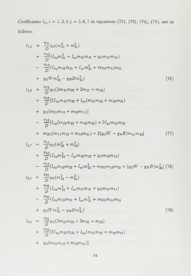
Coefficients kj,i = 1,2, 3 j = 5,6,7 in equations (72), (73), (74), (75), are as
follows:
7"H / 2 . 2 \
h,5 = -^yG{m3l + m 21 )
+ -jrilxyml-L + Iyzm 3im 2 i + yGm 2imn )
- —{Ixym3im 2 i + Iyzmli + myGmum 3 i
+ VG^rn\x-yBBm\ x ) (76)
*i,6 = —yG(2m 3im 32 + 2m 2 i + m 22)
+ — [2Ixym2\mz2 + Iyz('m3im22 + "232^21)
+ ?/G(^2l7ni2 + 7n22^1l)]
££-10
- — \Ixy{mzim 22 + m 32m 2i) + 2/y2m 2im 22
+ myG(mnm 32 + mi2m31 ) + 2(yGW - yBB)m AxmA2 ] (77)
7
an / 2 , 2 \
'1,7 = -jrVG{™<32 + m22 )
+ — {hyml2 + Iyzm32rn 22 + yGm 22rni2)
- —[Ixym32m22 + Iyzrnl2 + myGmi2m 32 + (yGW - yBB)ml2 ] (78)
,
a21 / 2 . 2 \
^2,5 = -^-yc(m 31 + m 21 )
a22 / r 2 r \+ -jr\Ixy™> 31 + iyZm31m2i + yG"i2imn)
- — (iiym 3im2i + Iyzm21 + myGmiim 3 i
+ ycWm 2^ - yBBm 2
41 ) (79)
^2,6 = —yG(2m 31m 32 + 2m 2 i + m 22)
+ —[2Ixym 3im 32 + Iyz(m 3im22 + m 32m 2i)
+ 2/^(^21^12 + ^22^11)]
34

- —[Ixy{™>3im22 + m 32m2i) + 2IyZm 2im 22
+ myG(mum 32 + mi2m3i) + 2{yGW - yBB)m4im42} (80)
^21 / 2 2 \
^2,7 = -jyyG{rn32 + m 22 )
+ -jr(Ixym\2 + Iyzmwm22 + yGm22mi2)
- —[Ixyms2m22 + Iyzml2 + myGmi2m 32 + {vgW ~ VBB)m\2 \ (81)
^31 / 2 2 \
^3,5 = -jj-yG{m 3l + m 21 )
+ -jrilxymzi + A/-*m 3im 2i + yG^2i^n)
Q33
D(i"iyr72 3im2i + Iyzm 21
4- myGmnm 3i
+ yGWm^-yBBm2^) (82)
/7 0-1
^3,6 = —yG(2m31m32 + 2m2i + m22 )
+ — [2ixym3im 32 + 7y2 (m31m 22 + m 32m 2 i
)
+ ^(^21^12 + ^22^11)]
/Too
- —[4y(^31^22 + rn 32m 2i ) + 2Iyzm 2im 22
+ myG(mnm 32 + m12m3i) + 2(yGW - 2/5^)^41^42] (83)
^3,7 = -jyyG{m32 + m22 )
+ —(Ixyml2 + Iyzm32m 22 + yGm 22m l2 )
- —[Ixym 32m 22 + Iyzm\2 + myGm l2m 32 + (yG^ - yBB)m\2 ] (84)
Then equations (61), (62), can be written as follows:
23 = P1 z3 + d3 + e 3 (85)
Z4 = jP2 24 + <^4 + e4 (^6)
35
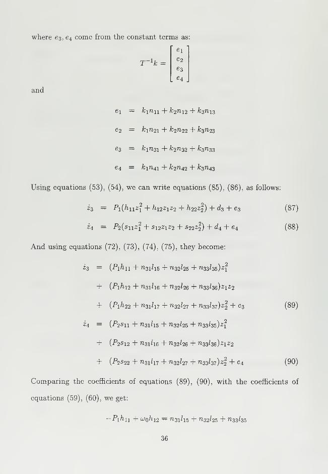
where e3 , e4 come from the constant terms as:
T~ lk =
e 4
and
ei
e2
e3
e4
= kinu + k2ni2 + hnu
= feiTl2i + fc2n22 + k3n23
= fei7i3i + /c2n32 + k3n33
— k\n±\ + k2ri42 + k3n A3
Using equations (53), (54), we can write equations (85), (86), as follows:
i3 = Pi(hn zl + hi2ziz2 + h22Z%) + d3 + e3 (87)
za — P2{s\\z1 + sriz\Z2 + si2z\) + d4 + e 4 (88)
And using equations (72), (73), (74), (75), they become:
i3 = (Pi/in + n 31 /i5 + n 32 /25 + ^33/35)2?
+ {Pihu + n 3ihe + n 32 l26 + n33 l36 )ziz2
+ {P\h22 + n3il 17 + n32 l27 + n33 l37 )z% + e3 (89)
i4 = (P2sn + n3i/ 15 + n32 /25 + n33 l35 )zj
+ (P2S12 + ^31^16 + ^32^26 + n33 l36 )z1 Z2
+ (P2S22 + ^31^17 + 7W27 + ^33^37)^1 + e4 (90)
Comparing the coefficients of equations (89), (90), with the coefficients of
equations (59), (60), we get:
-Pi /in + u;ohi2 = 7131Z15 + 7*32/25 + 7*33/35
36
-2oJ hn - P\h\2 + 2<Vo^22 = ^31^16 + ™32^26 + n33 l36
-LO hi2 - P\h 22 = ^31/17 + n 32 /27 + ™33^37
Solution of the above 3x3 linear system of equations, gives us coefficients tin,
ft-12, ^22-
Also in the same way:
-P2S11 + co si2 = n4i/i5 + n42 /25 + ^43^35
-2l0qSu - P2S12 + 2u) S22 = n4 ilie + n42 /26 + ^43^36
-UQSi2 - P2S22 = rt4iln + 7142^27 + ^43^37
Solution of the above 3x3 linear system of equations, gives us coefficients sn,
512, 522-
E. AVERAGING
In this part of our analysis we are going to take into account the third order
terms of equation (52):
Where,
T- lG {z\Tz) =
hhhU
h
h
h
nuG {?{Tz) + n l2G2 (3)(Tz) + n 13G 33)(T z)
n 21G?\Tz) + n22G 2 (3)(Tz) + n 23G 33)(Tz)
-0) (3),- n 31G\*\Tz) + n32G 2 (S)(Tz) + n 33G 3°'(Tz)
(91)
(92)
(93)
37
U = n4lG^(Tz)+n42G2(S)(Tz)+n43G {
z
3\T:z) (94)
If we substitute equations (68), (69), (70), (71) and the expressions for G\,
G 2 , Gz into equations (91) throuh (94), we get:
h = nn {h\z\ + luzjz2 + I13Z1Z2 +/l4^)
+ nnihiZi + I22Z1Z2 + hzz\z2 + I24Z2)
+ ni3 (l3izl + Iz2z\z2 + hzz\z\ + Z34z|) (95)
/2 = "21^11^1 +112*1*2 + hzZ\zl + I14Z2)
+ n22\l2iZi + I22Z1Z2 + I23Z1Z2 + I24Z2)
+ ™23^31-Z? + ^32^1^2 + h&\z\ + ^34^|) (96)
h = n3i(hiz% + li2zlz2 + h3Ziz% + luz%)
+ ^32(^21^! + ^22^x22 + I23Z1Z2 + I24Z2)
+ n>33(hizl + h2z\z2 + I33Z1Z2 + I34Z2) (97)
Ia — ^l^ll^l + l\2Z\Z2 + l\3Z\Z2 + I1AZ2)
+ n42 {l2izl + h2z\z2 + lvZZ\z\ + l2Az\)
+ n4Z {lzx z\ + hiz\z2 + hzz\z\ + 13az\) (98 )
From equation (52) and from the system matrix, the derivatives of the first
two modified coordinates, z\ and z,2 can be written as follows:
z\ — (a'e)zi-(ujo + uj'e)z2 + FFi(zi,Z2) (99)
i2 = (ljq + uj'e)zi + a'ez2 + FF2 (zi,Z2) (100)
where,
FF1 (z 1 ,z2 ) = di + /i+ei (101)
38

FF2 {zi, z2 ) = d2 + f2 + e2 (102)
If we combine equations (101) and (102) with equations (72) through (75),
and (95) through (98), we get:
FFi{zi, z2 ) = rn zf + ri2zjz2 + r 13z1Z2+ru zl
+ PnZi + P\2z\z2 + pizzl + ei
FF2 {zi,z2 ) = r21z\ + r22z\z2 + r2Zzx z\ + r2^z\
+ V2iz\ + p22ziz2 + p23z% + ei
(103)
(104)
where coefficients r*j and pij are:
rn = nnZn + ni2 l2 i + TI13/31
ru = n\
r\z = ni
r 14 = ni
7"2i = n2
r22 = n2
J"23 = ™2
r24 = n2
h2 + ni 2 l22 + n 13 /32
^13 + ™12^23 + "13^33
*14 + ™12^24 + ™ 13^34
hi + ^22^21 + ™23^31
^12 + ^22^22 + ^23^32
^13 + n 22^23 + n23^33
*14 + ^22^24 + ™23^34
or generally,
Uj = nnhj + n i2 l2j + n i3 /3j i = 1, 2 j = 1, 2, 3,
4
(105)
also,
Pll = "11*15 + "12*25 + "13*35
39

Pu = nu lis + 77,12/26 + "-13/36
Pl3 = "ll/l7 + "12/27 + "13/37
P21 = "2l/l5 + "22/25 + "23/35
P22 = "2l/l6 + "22/26 + "23/36
P23 = "2l/l7 + "22/27 + "23/37
or generally,
Pij = nnhk + ni2l2k + nnhk i = 1,2 j = 1,2,3 k=j + 4 (106)
The coefficients Uj i = 1, 2, 3 j = 1, 2, 3, 4 are as follows:
Z11 = - -7- [-7-^(^o7n?i + 3£?imi 1m2i + S^miimg! + ^3^21)Z> 07
- -Fr["T^(^im ii + 3E2mi 1m 2 i + 3Ezmumli + E^m^)
u 07
+ i(xG^ - xBB)m\ x \ + ^(zgW - zBB)ml1 (107)
/12 = —^[-^(3£oran"n2 + 3£i(mi 1m 22 + 2miim 12m2i)D 67
+ 3 JE2(7ni2"i2i + 2m 2im227"n) + 3^37712^22) + -{W - £)3m41m42]
- —[-^(S^im^mw + 3E2{(ml lm 22 + 2mnm^m 21)D 67
+ 3^3 ((77112771 21 + 2m 21 77122771n) + 3E4m\ lm22)
+ ~{xGW -xBB)3ml 1m 42} + ^-(zGW -zBB)3ml l
m 42 (108)bD
/13 = -—[—^(3E 7"n7"?2 + 3 -£;i(m i2rn 2i + 2mnmi 2m 22)JJ 07
+ 2>E2{m\2mu + 2m 2\m22rriyi) + 3E^m2\m\2 )
+ ~{W - B)3m 4lm242 }
D
40
- -T-[-r^-(SEimnml2 + 3E2 (ml2m 21 + 2m V[m vlm 22 )D 07
+ 3Es(ml2mn + 2m 2im 22mi2 ) + 3E4m2im 2l
2 )
+ -^{xGW - xBB)3m4lm 242 \ + ^{zGW - zBB)3m4lm 2
42 (109)
lU = Fr[-T^(^07n?2 + 3^1771^77121 + 3^2^12771^ + £3^22)JJ 07
+ i(W-B)mj2]
- —[-T-^-{Eim\2 + 3E2m 2
um 2 i + 3Ezm l2m 2
22 + E4m\2 )u 07
+ -(xGW - xBB)m\2 ] + ^{zGW - zBB)m\2 (110)OJJ
hi = —^[^{Eoml 1 + 3Eiml 1m2i + 3E2miim21 +E3m2i)
JJ 07
+ i(W- B)m 3
4l ]
- -Trl-r-^iEimli + 3E2m\lm 2 i + Si^mum™ + £4^21)
JJ 07
+ \{xGW - xbB^W) + ^r(zGW - zBB)m 341 (111)
o oJJ
hi - —^-[-7-^(3^0^11^12 + 3^1(777^77222 + 2mnmi27n2i)V 07
4- 3^2(^112^21 + 27772177722mn) + 3Ezm\ lrri2i) + -{W — B^m^m^
- -r-[-rJL (3^imi 1mi2 + 3£2((m?i™22 + 2mii777i2m 2i)V 07
+ 3E3((mi27772i + 2m 2im 22mn) + 3E4ml 1m 22)
+ l(xGW -xBB)3m2
1m 42 } + ^-{zGW -zBB)3m 2
41m42 (112)6 oD
*23 = rr[-7T-^(3^0"7ll7ri?2 + 3£;i(777i2m21 +2miimi277722)D 07
+ 3E2 (77722^11 + 2777217772277712) + 3£^37772l77722)
+ -{W - B)3m 4xm242 \
- -=-[-r^-{3Eim llm\2 + 3E2{ml2m 21 + 2miimi2m 22 )D 67
41

+ 3Ez{m\2rnii + 2m 2\m 22m\2 ) + 3E4m 2im\2 )
+ ~{xgW - xBB)3m4im42 \ + -—(zGW - ZBB)3m 4im 42 (113)o bJJ
l24 = -—^[—^-(Eornl2 + 3Eirn2
nm 2 i + 3E2mi2ml2 + E3ml2 )JJ 07
+ \{W-B)m\2 )
- -rr[-^{Eim\2 + 3E2m\ lm 2l + 3E3m l2m 2
22 + E4ml2 )JJ 07
+ \{xGW ~xBB)m\2 } + ^-{zGW -zBB)m\2 (114)o oJJ
kl = Tr[-rJL
(EOm ll + 3^1771^77121 + 3^27711177121 + i?3™2l)
L* 07
+ ±(W-B)m 341 ]
- -=-[-rJL (Eim ii + 3 JE2"iii77i2i + 3Ezmum\ l + ^4^21)D 07
+ ^(xGW - xBB)m\1 ) + ^(zGW - zBB)m3
4l (115)
J32 = —^[-^(3Eoml 1mi2 + 3Ei(mj1m22 + 2miim 12rn 21 )D 07
+ 3E2{mi2m\ l + 2m2\m^mu) + 3E3m2 1m22) 4- -(W — B)3m41m42]
- -77 [-rJL (3Eiml 1mi2 + 3E2({m\
lm 22 + 2miimi2m 2i)D 07
+ 3E3((mi2m21 + 277121777,2277211 ) + 3£4 777, 21 777,22)
-(xGW - xBB)3m241m42 } +—
o oL>+ -(xgW - x BjB)3m4 1
m42] + —— {zGW - zBB)3ml lm 42 (116)
^33 = -^\-^{ZEQmum\2 + 3Ei(rn\2rn2\+2rnu rni2rri22)
D 07
+ 3.E2(777,22m ll + 2777,217712277712) + 3^3777,2l7n 22 )
+ -{W - B)3m4lm 242 ]
- -^[-rJL{ZEimnm\2 + 3E2(ml2m 2 i + 2mnmi2m 22)JJ 07
+ 3 £3(777, 22 777 11 + 277l2l77222777l2) + SE^TTT^lTTT^)
42
+ -(xGW -xBB)3m 4lm 2
42 } + ^{zGW -zBB)3m4lm 242 (117)
l34 = --—[—^-(Eornl2 + 3Eimll rn2i + 3E2rni2rnl2 + E3rnl2 )D 07
+ \{W-B)mU
- -—\—^{Eim\2 + 3E2ml lm 2i + 3E3m x2m\2 + E4m\2 )U 07
+l-{xGW - xBB)m\2 ] + ^(zGW - zBB)m\2 (118)
The next step is to introduce polar coordinates in the form:
zi = Rcos6 (119)
z2 = Rs\n9 (120)
We use polar coordinates, because it is easier in this way to investigate the
existence of limit cycles.
Substituting equations (119), (120), into equations (99), (100), we get:
RcosO - R{smd)6 = (co + co'e)R cos 9 + a'eR sin 9 +
Pl {9)R3 + Q l {9)R
2 + e l (121)
Rsin9 + R(cos9)9 = (co + u'e)R cos 6 + a'eR sin 6 +
P2{9)R3 + Q 2 {e)R
2 + e2 (122)
where,
P\{0) = rn cos39 + ri2 cos
29 sin 9 + rl3 cos 9 sin
29 + r 14 sin
39 (123)
Q Y {9) = pn cos2 0+pi2cos0sin0+p13 sin
2(124)
p2 {9) = r21 cos39 + r22 cos
2sin 9 + r23 cos 9 sin
2 + r24 sin39 (125)
£2(0) = P2icos29 +p22 cos9sin9 +p23 sm
29 (126)
43

If we multiply equation (121) by cos# and equation (122) by sin#, and add
the two resulting equations, we get:
R = a'eR + P(9)R 3 + Q{9)R2 + (e l cos 9 + e2 sin 9) (127)
where,
P(9) = Pi(9) cos 9 +
P
2 {9) sin
9
(128)
Q(9) = Qi(9) cos 9 + Q 2 (9) sin 9 (129)
Equation (127) contains one variable that varies slowly in time (R) and a fast
variable (9).
If we average this equation over one complete cycle in 9, from to 27r,
equation (127) becomes:
R = a'eR + KR3 + LR2 + M (130)
where,
1 r2nK = — / P{9)d9Z7T JO
I,,
.
= -(3r-n +ri3 + r22 + 3r24 (131)
i-2-k
/ Q(9)d9 (132)Jo
1 f27r
2tt
1 /^M = — / ei cos 9 d92tt 7o
1 /27r
+ — / e 2 sin#d0
= |l[sin^-|H-[cos(?]r
= (133)
44
Finally equation (135) becomes:
R = a'eR + KR 3(134)
F. LIMIT CYCLE ANALYSIS
At steady state R = 0,and equation (134) becomes:
= R(ae + KR2) (135)
Equation (135) has two solutions. The first solution is R = 0. This is the
trivial solution and it does not give us much information.The second solution
is:
R =y— (l36)
This solution gives us a limit cycle of constant amplitude R in the zi, 22
cartesian coordinate system.This limit cycle exists if the quantity inside the
square root is possitive, or
-n't> (137)K
Condition (137) is necessary for the amplitude of the limit cycle, R, to be a
real number.
In our case a' is always negative, because for constant xq, as we decrease
e (Figure 1), the real part of the critical pair of eigenvalues increases, due to
further loss of stability. In other words we can say that:
a' < (138)
45
From conditions (137), (138) we see that the existence of the limit cycles
depends on the value of parameter K . We can see that:
• If K < 0, periodic solutions exist for e < or zq — zqc< or zq < zq
c ,
and they are stable.
• If K > 0, periodic solutions exist for e > or zq — zqc> or zq > zq
c ,
and they are unstable.
The characteristic root of equation (134) in the vicinity of (136) is:
/3 = -2a'e (139)
The sign of this characteristic root, assigns the stability of the periodic solu-
tions.
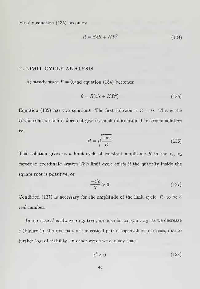
G. RESULTS AND DISCUSSION
Typical results in terms of the nonlinear stability coefficient K are pre-
sented in Figures 3 through 6. The stability coefficient K is shown in its
normalized form as K 7 (Papadimitriou, 1994). Figure 3 shows K versus
the LCG/LCB separation distance xq (in ft) for a given vehicle speed and for
different values of the drag coefficient. It can be seen that K is everywhere
negative, which means that all bifurcations to periodic solutions are super-
critical. Higher values of the drag coefficient result in stronger supercritical
bifurcations which means that the corresponding limit cycle amplitudes will
be smaller.
46
x 103
i 1
-1
-2
<-3
i*-4
-5
-6
0.1
:
: 0.3!
i 0.5^
i 0.7i! 0.9;
7 i 1 '
0.2 0.4 0.6 0.8 1
XG1.2 1.4 1.6 1.8
Figure 3: K • 7 versus xg for U — 5 ft/sec and different values of Cd
x 101
1 1 1
-1
23.5
5
6.5l__..
8...
f-2
2<XZ-3
-4
-5
a 11 —1
0.2 0.4 0.6 0.8 1 1.2 1.4 1.6 1.8 2XG
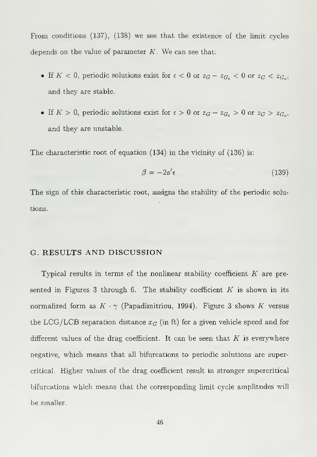
Figure 4: K 7 versus xg for Cn =0.5 and different values of U (ft/sec)
47

1.5
1-
b> 0.5S
J2
-0.5-
-1
1 i i r i i
:zgZG
=0.04=0.05
I... 11.
Ill4..J.JI!
1•
ii
i i
50 100 150 200 250 300 350 400 450 500Time (sec)
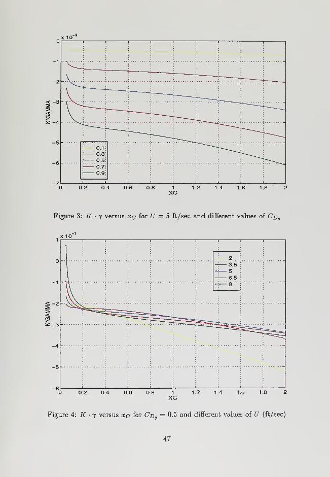
Figure 5: Simulation results (0, t) for Cn = 0.5, U = 5 ft/sec, and xq = 1 ft
4-
3 -
? 2h
S 1
I °
o '
'IZi-2h
-3-
-4-
-50.02 0.025 0.03 0.035 0.04 0.045 0.05 0.055 0.06
ZG
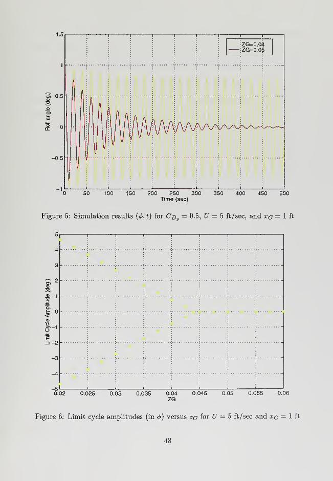
Figure 6: Limit cycle amplitudes (in 0) versus zq for (7 = 5 ft/sec and xg — 1 ft
48

Figure 4 shows K versus xq for a given drag coefficient and for different
forward speeds. It can be seen that the bifurcations are supercritical with the
possible exception of large speeds and small xq. This means that it is possible
for a properly trimmed vehicle at relatively high speeds to experience an oscil-
latory behavior even before stability is lost. This demonstrates a destabilizing
effect which could not have been predicted by linear techniques.
Figures 5 and 6 shows numerical simulation results which confirm the theo-
retical predictions. Both figures correspond to a supercritical bifurcation case
and they show a continuous increase in limit cycle amplitudes as the bifurca-
tion point is crossed.
49

50
V. CONCLUSIONS AND RECOMMENDATIONS
This thesis presented a comprehensive nonlinear study of straight line sta-
bility of motion of submersibles in coupled sway/yaw/roll motions under open
loop conditions. Primary loss of stability was shown to occur in the form of
Hopf bifurcations to periodic solutions. This loss of stability is characteristic
of the coupling of roll into sway and yaw and cannot be predicted by consid-
ering the uncoupled motions. The critical point where instability occurs was
computed in terms of vehicle metacentric height, longitudinal separation of
the centers of buoyancy and gravity, and the forward speed. Analysis of the
periodic solutions that resulted from the Hopf bifurcations was accomplished
through Taylor expansions, up to third order, of the equations of motion. A
consistent approximation, utilizing the generalized gradient, was used to study
the non-analytic quadratic cross flow integral drag terms. The results indi-
cated that loss of stability occurs always in the form of supercritical Hopf
bifurcations with stable limit cycles. It was shown that this is mainly due to
the stabilizing effect of the drag forces at high angles of attack. Subcritical
bifurcations, however, with considerably higher limit cycle amplitudes may
develop for sufficiently high forward speeds and small LCG/LCB separations.
Simulation studies of these subcritical bifurcations along with the effects of
vertical plane coupling constitute recommendations for further research.
51

52

APPENDIX
The following is a list and description of the computer programs used in this
thesis. The programs are written in FORTRAN or MATLAB. Complete print-
outs of the programs follow after the list.
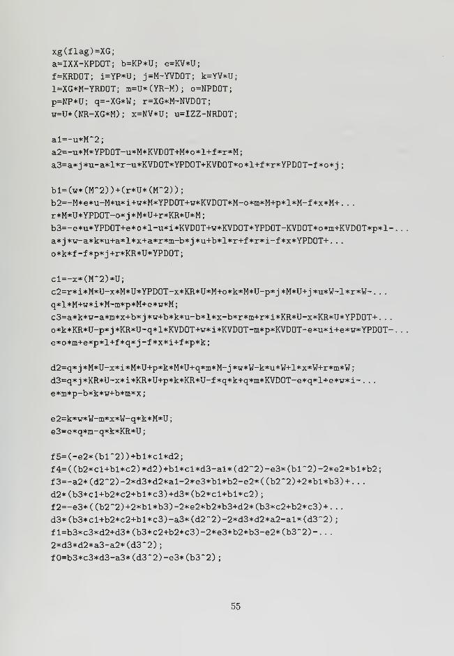
• STABILITY.M
MATLAB program for performing linear stability analysis.
• SIM.M
MATLAB program and functions for numerical simulation.
• HOPF.FOR
FORTRAN program for calculating the nonlinear stability analysis coef-
ficient K . It requires data from STABILITY.M and standard numerical
linear algebra subroutines.
53
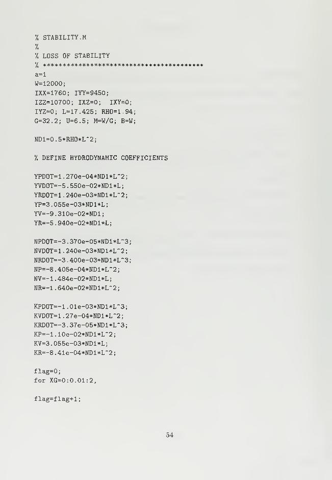
•/. STABILITY.
M
%
'/. LOSS OF STABILITY
yo *****************************************
a=l
W=12000;
IXX=1760; IYY=9450;
IZZ=10700; IXZ=0; IXY=0;
IYZ=0; L=17.425; RH0=1.94;
G=32.2; U=6.5; M=W/G; B=W;
ND1=0.5*RHO*L~2;
•/. DEFINE HYDRODYNAMIC COEFFICIENTS
YPDOT=l . 270e-04*NDl*L~2
;
YVD0T=-5 . 550e-02*NDl*L
;
YRDOT=l . 240e-03*NDl*L~2
;
YP=3.055e-03*NDl*L;
YV=-9.310e-02*NDl;
YR=-5.940e-02*NDl*L;
NPD0T=-3 . 370e-05*NDl*L~3
;
NVDOT=l . 240e-03*NDl*L~2
;
NRD0T=-3 . 400e-03*NDl*L"3
;
NP=-8 . 405e-04*NDl*L~2
;
NV=-1.484e-02*NDl*L;
NR=-1 . 640e-02*NDl*L~2
;
KPDOT=-l .01e-03*NDl*L"3;
KVDOT=l . 27e-04*NDl*L'2
;
KRDOT=-3 . 37e-05*NDl*L~3
;
KP=-1 . 10e-02*NDl*L~2
;
KV=3.055e-03*NDl*L;
KR=-8.41e-04*NDl*L~2;
flag=0;
for XG=0:0.01:2,
flag=flag+l;
54
xg(flag)=XG;
a=IXX-KPDOT; b=KP*U; e=KV*U;
f=KRDOT; i=YP*U; j=M-YVDOT; k=YV*U;
1=XG*M-YRD0T; m=U*(YR-M); o=NPDOT;
p=NP*U; q=-XG*W; r=XG*M-NVDOT;
w=U* (NR-XG*M) ; x=NV*U; u=IZZ-NRDOT;
al=-u*M~2;
a2=-u*M*YPD0T-u*M*KVD0T+M*o*l+f*r*M;
a3=a*j*u-a*l*r-u*KVD0T*YPD0T+KVD0T*o*l+f*r*YPD0T-f*o*j;
bl=(w*(M~2) )+(r*U* (M~2) )
;
b2=-M*e*u-M*u*i+w*M*YPD0T+w*KVD0T*M-o*m*M+p*l*M-f*x*M+. .
.
r*M*U*YPDOT-o* j *M*U+r*KR*U*M
;
b3=-e*u*YPD0T+e*o*l-u*i*KVD0T+w*KVD0T*YPD0T-KVD0T*o*m+KVD0T*p*l-
a*j*w-a*k*u+a*l*x+a*r*m-b*j*u+b*l*r+f*r*i-f*x*YPDOT+. .
.
o*k*f-f*p*j+r*KR*U*YPDOT;
cl=-x*(M~2)*U;
c2=r*i*M*U-x*M*U*YPD0T-x*KR*U*M+o*k*M*U-p* j *M*U+j *u*W-l*r*W- . .
.
q*l*M+w*i*M-m*p*M+e*w*M;
c3=a*k*w-a*m*x+b* j *w+b*k*u-b*l*x-b*r*m+r*i*KR*U-x*KR*U*YPDOT+ . .
,
o*k*KR*U-p*j*KR*U-q*l*KVDOT+w*i*KVDOT-m*p*KVDOT-e*u*i+e*w*YPDOT-
e*o*m+e*p*l+f*q*j-f *x*i+f *p*k;
d2=q* j *M*U-x*i*M*U+p*k*M*U+q*m*M- j *w*W-k*u*W+l*x*W+r*m*W
;
d3=q*j*KR*U-x*i*KR*U+p*k*KR*U-f*q*k+q*m*KVD0T-e*q*l+e*w*i-. .
.
e*m*p-b*k*w+b*m*x
;
e2=k*w*W-m*x*W-q*k*M*U
;
e3=e*q*m-q*k*KR*U
;
f5=(-e2*(bl"2))+bl*cl*d2;
f4=((b2*cl+bl*c2)*d2)+bl*cl*d3-al*(d2~2)-e3*(bl~2)-2*e2*bl*b2;
f3=-a2*(d2~2)-2*d3*d2*al-2*e3*bl*b2-e2*((b2~2)+2*bl*b3)+. .
.
d2*(b3*cl+b2*c2+bl*c3)+d3*(b2*cl+bl*c2);
f2=-e3*((b2~2)+2*bl*b3)-2*e2*b2*b3+d2*(b3*c2+b2*c3)+. .
.
d3*(b3*cl+b2*c2+bl*c3)-a3*(d2~2)-2*d3*d2*a2-al*(d3~2);
f I=b3*c3*d2+d3*(b3*c2+b2*c3)-2*e3*b2*b3-e2*(b3"2)-. .
.
2*d3*d2*a3-a2*(d3~2)
;
f0=b3*c3*d3-a3* (d3"2) -e3* (b3~2)
;
55
coef=[f5 f4 f3 f2 fl fO]
;
ZG=roots(coef )
;
tot(flag)=ZG(5,l);
end
plot (xg, tot) ,grid;
title ('ZG versus XG plot in the point of loss of stability')
xlabelCXG in ft');
ylabeK'ZG in ft');
56
•/. NON LINEAR SIMULATION PROGRAM
tO=0;
tfinal=500;
q=(l/180)*pi;
yO= [0 q] ;
[t,y]=ode45('vdpo2' ,tO,tf inal,yO)
;
figure(l) ,plot(t(: , 1) ,57. 29578*y( : ,4)) ,grid
title( 'plot of fi with time');
ylabel('fi') .xlabeK'time')
57

7. NON LINEAR SIMULATION PROGRAM
function yprime=vdpo2(t ,y)
W=12000;
IXX=1760; IYY=9450;
IZZ=10700; IXZ=0; IXY=0;
IYZ=0; L=17.425; RH0=1.94; ZB=0;
G=32.2; U=5; M=W/G; B=W; XB=0;
ZG=0.05; CD=0.5; YG=0;
XG=1; YB=0;
ND1=0.5*RH0*L~2;
7, DEFINE HYDRODYNAMIC COEFFICIENTS
YPDOT=l . 270e-04*NDl*L~2
;
YVD0T=-5 . 550e-02*NDl*L
;
YRDOT=l . 240e-03*NDl*L~2
;
YP=3.055e-03*NDl*L;
YV=-9.310e-02*NDl;
YR=-5 . 940e-02*NDl*L
;
NPDOT=-3 . 370e-05*NDl*L~3
;
NVDOT=1.240e-03*NDl*L~2;
NRDOT=-3 . 400e-03*NDl*L"3;
NP=-8 . 405e-04*NDl*L~2
;
NV=-1.484e-02*NDl*L;
NR=-1.640e-02*NDl*L~2;
KPDOT=-l . Ole-03*ND1*L~3
;
KVDOT=l . 27e-04*NDl*L~2
;
KRD0T=-3 . 37e-05*NDl*L~3
;
KP=-1 . 10e-02*NDl*L~2
;
KV=3.055e-03*NDl*L;
KR=-8.41e-04*NDl*L~2;
D=((M-YVDOT)*(IZZ-NRDOT)*(IXX-KPDOT)) . .
.
-((M-YVDOT)*(IXZ-KRDOT)*(-IXZ-NPDOT)) . .
.
-((M*XG-NVDOT)*(M*XG-YRDOT)*(IXX-KPDOT)) .
.
+ ( (M*XG-NVDOT) * (IXZ-KRDOT) * (-M*ZG-YPDOT) )
.
+ ( (-M*ZG-KVDOT) * (M*XG-YRDOT) * (-IXZ-NPDOT)
)
58
- ( (-M*ZG-KVDOT) * (IZZ-NRDOT) * (-M*ZG-YPDOT) )
;
EVALUATE TRANSFORMATION MATRIX OF EIGENVECTORS
All= ( (IZZ-NRDOT) * (IXX-KPDOT) ) - ( (IXZ-KRDOT) * (-IXZ-NPDOT) )
;
A12= ( (-M*XG+YRDOT) * (IXX-KPDOT) ) + ( ( IXZ-KRDOT) * (-M*ZG-YPDOT) )
;
A13= ( (M*XG-YRDOT) * (-IXZ-NPDOT) ) - ( (IZZ-NRDOT) * (-M*ZG-YPDOT) )
;
A21= ( (-M*XG+NVDOT) * (IXX-KPDOT) )+( (-M*ZG-KVDOT) * (-IXZ-NPDOT) )
;
A22= ( (M-YVDOT) * (IXX-KPDOT) ) - ( (-M*ZG-KVDOT) * (-M+ZG-YPDOT) )
;
A23= ( (-M+YVDOT) * (-IXZ-NPDOT) ) + ( (M*XG-NVDOT) * (-M*ZG-YPDOT) )
;
A31= ( (M*XG-NVDOT) * (IXZ-KRDOT) ) - ( (-M*ZG-KVDOT) * (IZZ-NRDOT) )
;
A32= ( (-M+YVDOT) * (IXZ-KRDOT) ) + ( (-M*ZG-KVDOT) * (M*XG-YRDOT) )
;
A33= ( (M-YVDOT) * (IZZ-NRDOT) ) - ( (M*XG-NVDOT) * (M*XG-YRDOT) )
;
7.
'/
F
F
F
F
F
F
F
F
F
F
F
F
F
F
F
F
'/.
7.
"/.
(1,1
(1,2
(1,3
(1,4
(2,1
(2,2
(2,3
(2,4
(3,1
(3,2
(3,3
(3,4
(4,1
(4,2
(4,3
(4,4
= (A11*YV*U+A12*NV*U+A13*KV*U) /D
;
=(A11*(YR*U-M*U)+A12*(-M*XG*U+NR*U)+A13*(M*ZG*U+KR*U))/D;
=(A11*YP*U+A12*NP*U+A13*KP*U)/D;
=0;
= (A21*YV*U+A22*NV*U+A23*KV*U) /D
;
= (A21* (YR*U-M*U) +A22* (-M*XG*U+NR*U) +A23* (M*ZG*U+KR*U) ) /D
;
=(A21*YP*U+A22*NP*U+A23*KP*U)/D;
=0;
= (A31*YV*U+A32*NV*U+A33*KV*U) /D
;
= (A31* (YR*U-M*U) +A32* (-M*XG*U+NR*U) +A33* (M*ZG*U+KR*U) ) /D
;
= (A31*YP*U+A32*NP*U+A33*KP*U) /D
;
=0;
=0
=0
= 1
=0
CALCULATION OF THE INTEGRATION TERMS Ei
7. DEFINE THE LENGTH
7. ALL IN FEET.
XL(1)=-105.9/12;
XL(2)=-104.3/12;
XL(3)=-99.3/12:
XL(4)=-94.3/12:
XL(5)=-87.3/12:
XL(6)=-76.8/12:
X AND HEIGHT H TERMS FOR THE INTEGRATION
59
XL(7)=
XL(8)=
XL(9)=
XL(10)
XL(ll)
XL(12)
XL(13)
XL (14)
XL(15)
XL(16)
XLC17)
XL(18)
-66.3/12;
-55.8/12;
72.7/12;
=79.2/12
=83.2/12
=87.2/12
=91.2/12
=95.2/12
=99.2/12
=101.2/12
=102.1/12
=103.2/12
HT(1)=
HT(2)=
HT(3)=
HT(4)=
HT(5)=
HT(6)=
HT(7)=
HT(8)=
HT(9)=
HT(10)
HT(ll)
HT(12)
HT(13)
HTC14)
HT(15)
HT(16)
HT(17)
HT(18)
0;
2.28/12;
8.24/12;
13.96/12;
19.76/12;
25.1/12;
29.36/12
31.85/12
31.85/12
=30.00/12
=27.84/12
=25.12/12
=21.44/12
=17.12/12
=12.0/12
=9.12/12
=6.72/12
=0;
for 1-1:18,
VECl(i)=HT(i)*(y(l)+XL(i)*y(2))*(abs(y(l)+XL(i)*y(2)));
VEC2(i)=HT(i)*(y(l)+XL(i)*y(2))*(abs(y(l)+XL(i)*y(2)))*XL(i);
end
OUT=0
;
for j=l:17,
0UTl=0.5*(VECl(j)+VECl(j+l))*(XL(j+l)-XL(j));
0UT=0UT+0UT1;
end
60
IV=CD*OUT;
OUT=0
;
for 3-1:17,
0UT2=0.5*(VEC2(j)+VEC2(j+l))*(XL(j+l)-XL(j));
0UT=0UT+0UT2;
end
IR=CD*0UT;%================================================================
yprime=[F(l,l)*y(l)+F(l,2)*y(2)+F(l,3)*y(3)+F(l,4)*y(4)+. .
.
(All/D)*(YG*(y(3)-2+y(2)-2)-IV+(W-B)*sin(y(4)))+. .
.
(A12/D)*(IXY*y(3)-2+IYZ*y(3)*y(2)+YG*y(l)*y(2)-IR+(XG*W-XB*B)*sin(y(4)))+.
(A13/D)*(-IXY*y(3)*y(2)-IYZ*y(2)"2-M*YG*y(l)*y(3)+(YG*W-YB*B)*cos(y(4)) . .
.
-(ZG*W-ZB*B)*sin(y(4))); . .
.
F(2,l)*y(l)+F(2,2)*y(2)+F(2,3)*y(3)+F(2,4)*y(4)+...
(A21/D)*(YG*(y(3)~2+y(2)~2)-IV+(W-B)*sin(y(4)))+. .
.
(A22/D)*(IXY*y(3)~2+IYZ*y(3)*y(2)+YG*y(l)*y(2)-IR+(XG*W-XB*B)*sin(y(4)))+.
(A23/D)*(-IXY*y(3)*y(2)-IYZ*y(2)-2-M*YG*y(l)*y(3)+(YG*W-YB*B)*cos(y(4)) . .
.
- (ZG*W-ZB*B) *sin(y (4) ));...
F(3,l)*y(l)+F(3,2)*y(2)+F(3,3)*y(3)+F(3,4)*y(4)+...
(A31/D)*(YG*(y(3)~2+y(2)~2)-IV+(W-B)*sin(y(4)))+. .
.
(A32/D)*(IXY*y(3)~2+IYZ*y(3)*y(2)+YG*y(l)*y(2)-IR+(XG*W-XB*B)*sin(y(4)))+.
(A33/D)*(-IXY*y(3)*y(2)-IYZ*y(2)-2-M*YG*y(l)*y(3) + (YG*W-YB*B)*cos(y(4)) . . .
-(ZG*W-ZB*B)*sin(y(4))) ; . .
.
l*y(3)];
61
C HOPF.FOR
C
C HOPF BIFURCATIONS PROGRAM
C
IMPLICIT DOUBLE PRECISION (A-H.O-Z)
REAL*8 L , IYY , M , YPDOT , YVDOT , ND1 , YRDOT
REAL*8 YP , YV , YR , NPDOT , NVDOT , NRDOT , NP , NV , NR
REAL*8 GAMA , U , KVDOT , KRDOT , KPDOT ,
D
REAL*8 E0,E1,E2,E3,E4,XG,ZG,KR,KP,KV,XG1,ZG1
C
REAL*8 M11,M12,M13,M14,M21,M22,M23
REAL*8 M24 , M31 , M32 , M33 , M34 , M41 , M42 , M43 , M44
REAL*8 N11,N12,N13,N14,N21,N22,N23,N24
REAL*8 N31,N32,N33,N34,N41,N42,N43,N44
REAL*8 L11,L12,L13,L14,L21,L22,L23,L24,L31
REAL*8 L32 , L33 , L34 , L15 , L16 , L17 , L25 , L26 , L27 , L35
REAL*8 L36 , L37 , L1A , L2A , L3A , L4A , L5A , L6A , L7A , L8A , L9A
REAL*8 LlOA , L11A , L12A , LI , L2 , L3 , L4 , L5 , L6 , L7
REAL*8 L8,L9,R11,R12,R13,R14,R21,R22,R23,R24
REAL*8 P11,P12,P13,P21,P22,P23
C
DIMENSION F(4,4) ,T(4,4) ,TINV(4,4) ,FV1(4) , IV1 (4) ,YYY(4,4)
DIMENSION WR(4),WI(4),TSAVE(4,4) ,TLUD(4,4) , IVLUD(4) ,SVLUD(4)
DIMENSION ASAVE(4,4) ,A2(4,4) ,XL(18) ,HT(18) ,ZGG(197) ,FF(4,4)
DIMENSION VECO ( 18) , VEC1 ( 18) , VEC2 ( 18) , VEC3 ( 18) , VEC4 ( 18) , XGG ( 197)
C
INTEGER I,J,K
C
OPEN ( 20 ,FILE=' HOPF. RES' , STATUS= ' OLD '
)
OPEN (21,FILE='DATA.DAT' , STATUS= ' OLD '
)
OPEN (23,FILE='H0PF1.RES' , STATUS= » OLD '
)
OPEN (25 , FILE= ' H0PF2 . RES'
, STATUS= ' OLD '
)
C
WEIGHT=12000.0
IXX =1760.0
IYY =9450.0
IZZ =10700.0
IXZ =0.0
IXY =0.0
IYZ =0.0
L =17.425
RHO = 1.94
62

WRITE (*,*) ' ENTER CD'
READ (*,*) CD
G =32.2
XB =0.0
ZB =0.0
YG =0.0
YB =0.0
YDELTAR=0 .
DELTAR=0 .
NDELTAR=0 .
NPR0P=0 .
M= WEIGHT/G
B= WEIGHT
W=WEIGHT
U=8.0
ND1=0.5*RH0*L**2
C
C DEFINE HYDRODYNAMIC COEFFICIENTS
C
YPD0T=1 . 270E-04*ND1*L**2
YVD0T=-5 . 550E-02*ND1*L
YRD0T=1 . 240E-03*ND1*L**2
YP=3.055E-03*ND1*L
YV=-9.310E-02*ND1
YR=-5.940E-02*ND1*L
C
NPD0T=-3 . 370E-05*ND1*L**3
NVD0T=1 . 240E-03*ND1*L**2
NRD0T=-3 . 400E-03*ND1*L**3
NP=-8 . 405E-04*ND1*L**2
NV=-1 .484E-02*ND1*L
NR=-1 . 640E-02*ND1*L**2
C
KPD0T=-1 . 01E-03*ND1*L**3
KVD0T=1 . 27E-04*ND1*L**2
KRD0T=-3 . 37E-05*ND1*L**3
KP=-1 . 10E-02*ND1*L**2
KV=3.055E-03*ND1*L
KR=-8 . 41E-04*ND1*L**2
C
C DEFINE THE LENGTH X AND HEIGHT H TERMS FOR
C THE INTEGRATION, ALL IN FEET.
63

XL( 1)=-105. 9/12.0
XL( 2)— 104.3/12.0
XL( 3)=-99. 3/12.0
XL( 4)=-94. 3/12.0
XL( 5)=-87. 3/12.0
XL( 6)=-76. 8/12.0
XL( 7)=-66. 3/12.0
XL( 8)=-55. 8/12.0
XL( 9)=72. 7/12.0
XL(10)=79. 2/12.0
XL(11)=83. 2/12.0
XL(12)=87. 2/12.0
XL(13)=91. 2/12.0
XL(14)=95. 2/12.0
XL(15)=99. 2/12.0
XL(16)=101. 2/12.0
XL(17)=102. 1/12.0
XL(18)=103. 2/12.0
HT( 1)= 0.000
HT( 2)= 2.28/12.0
HT( 3)= 8.24/12.0
HT( 4)= 13.96/12.0
HT( 5)= 19.76/12.0
HT( 6)= 25.1/12.0
HT( 7)= 29.36/12.0
HT( 8)= 31.85/12.0
HT( 9)= 31.85/12.0
HT(10)= 30.00/12.0
HT(11)= 27.84/12.0
HT(12)= 25.12/12.0
HT(13)= 21.44/12.0
HT(14)= 17.12/12.0
HT(15)= 12.0/12.0
HT(16)= 9.12/12.0
HT(17)= 6.72/12.0
HT(18)= 0.00
DO 104 K = 1,18
VECO(K)=HT(K)
VEC1(K)=XL(K)*HT(K)
64
VEC2 (K) =XL (K) *XL (K) *HT(K)
VEC3 (K) =XL (K) *XL (K) *XL (K) *HT (K)
VEC4 (K) =XL (K) *XL (K) *XL (K) *XL (K) *HT (K)
104 CONTINUE
CALL TRAP(18,VEC0,XL,E0)
CALL TRAP(18,VEC1,XL,E1)
CALL TRAP(18,VEC2,XL,E2)
CALL TRAP(18,VEC3,XL,E3)
CALL TRAP(18,VEC4,XL,E4)
C
WRITE (*,*) » ENTER GAMA'
READ (*,*) GAMA
C=================================================================:
C READ THE CRITICAL VALUES FOR XG AND ZG FROM FILE DATA. DAT
C
XGG(1)=0.0
ZGG(1)=0. 016358083
DO 1 1=2,197
READ (21,*)XG,ZG
XGG(I)=XG
ZGG(I)=ZG
C==================================================================
C DETERMINE [F] COEFFICIENTS
C
D= ( (M-YVDOT) * (IZZ-NRDOT) * (IXX-KPDOT)
)
& - ( (M-YVDOT) * (IXZ-KRDOT) * (-IXZ-NPDOT)
)
& - ( (M*XG-NVDOT) * (M*XG-YRDOT) * (IXX-KPDOT)
)
& + ( (M*XG-NVDOT) * (IXZ-KRDOT) * (-M*ZG-YPDOT)
)
& + ( (-M*ZG-KVDOT) * (M*XG-YRDOT) * (-IXZ-NPDOT)
)
& - ( (-M*ZG-KVDOT) * (IZZ-NRDOT) * (-M*ZG-YPDOT)
)
C
All=( (IZZ-NRDOT) * (IXX-KPDOT) )-( (IXZ-KRDOT) * (-IXZ-NPDOT)
)
A12=((-M*XG+YRD0T)* (IXX-KPDOT) )+( (IXZ-KRDOT) * (-M*ZG-YPDOT)
)
A13= ( (M*XG-YRDOT) * (-IXZ-NPDOT) ) - ( (IZZ-NRDOT) * (-M*ZG-YPDOT)
)
A21= ( (-M*XG+NVDOT) * (IXX-KPDOT) ) + ( (-M*ZG-KVDOT) * (-IXZ-NPDOT)
)
A22= ( (M-YVDOT) * (IXX-KPDOT) ) - ( (-M*ZG-KVDOT) * (-M*ZG-YPDOT)
)
A23= ( (-M+YVDOT) * (-IXZ-NPDOT) ) + ( (M*XG-NVDOT) * (-M*ZG-YPDOT)
)
A31= ( (M*XG-NVDOT) * (IXZ-KRDOT) ) - ( (-M*ZG-KVDOT) * (IZZ-NRDOT)
)
A32= ( (-M+YVDOT) * (IXZ-KRDOT) ) +( (-M*ZG-KVDOT) * (M*XG-YRDOT)
)
A33= ( (M-YVDOT) * (IZZ-NRDOT) ) - ( (M*XG-NVDOT) * (M*XG-YRDOT)
)
C
F(1,1)=(A11*YV*U+A12*NV*U+A13*KV*U)/D
65
F(1,2)=(A11*(YR*U-M*U)+A12*(-M*XG*U+NR*U)+A13*(M*ZG*U+KR*U))/D
F(1,3)=(A11*YP*U+A12*NP*U+A13*KP*U)/D
F(1,4)=(A11*(W-B)+A12*(XG*W-XB*B)+A13*(-ZG*W+ZB*B))/D
F (2 , 1 ) = (A21*YV*U+A22*NV*U+A23*KV*U) /D
F (2 , 2) = (A21* (YR*U-M*U) +A22* (-M*XG*U+NR*U) +A23* (M*ZG*U+KR*U) ) /D
F(2 , 3) = (A21*YP*U+A22*NP*U+A23*KP*U) /D
F(2,4)=(A21*(W-B)+A22*(XG*W-XB*B)+A23*(-ZG*W+ZB*B))/D
F (3 , 1) = (A31*YV*U+A32*NV*U+A33*KV*U) /D
F (3 , 2) = (A31* (YR*U-M*U) +A32* (-M*XG*U+NR*U) +A33* (M*ZG*U+KR*U) ) /D
F(3 , 3) = (A31*YP*U+A32*NP*U+A33*KP*U) /D
F(3,4)=(A31*(W-B)+A32*(XG*W-XB*B)+A33*(-ZG*W+ZB*B))/D
F(4,l)=0.0
F(4,2)=0.0
F(4,3)=1.0
F(4,4)=0.0
EVALUATE TRANSFORMATION MATRIX OF EIGENVECTORS
DO 11 K=l,4
DO 12 J=l,4
ASAVE(K,J)=F(K,J)
12 CONTINUE
11 CONTINUE
CALL RG(4,4,F,WR,WI,1,YYY,IV1,FV1,IERR)
WRITE(23,1007)WR(1),WR(2) ,WR(3) ,WR(4)
CALL DSOMEG ( IEV , WR , WI , OMEGA , CHECK)
OMEGAO=OMEGA
DO 5 3=1,4
T(J,1)= YYY(J,IEV)
T(J,2)=-YYY(J,IEV+1)
5 CONTINUE
IF (IEV. EQ. 1.0) GO TO 13
IF (IEV. EQ. 2.0) GO TO 18
IF (IEV. EQ. 3.0) GO TO 14
STOP 3004
14 DO 6 J=l,4
T(J,3)=YYY(J,1)
T(J,4)=YYY(J,2)
6 CONTINUE
GO TO 17
18 DO 19 J=l,4
T(J,3)=YYY(J,1)
66
T(J,4)=YYY(J,4)
19 CONTINUE
GO TO 17
13 DO 16 J=l,4
T(J,3)=YYY(J,3)
T(J,4)=YYY(J,4)
16 CONTINUE
17 CONTINUE
C
C NORMALIZATION OF THE CRITICAL EIGENVECTOR
C
CALL NORMAL (T)
C
C INVERT TRANSFORMATION MATRIX
C
DO 2 K=l,4
DO 3 J=l,4
TINV(K,J)=0.0
TSAVE(K,J)=T(K,J)
3 CONTINUE
2 CONTINUE
CALL DLUD (4 , 4 , TSAVE , 4 , TLUD , IVLUD
)
DO 4 J=l,4
IF (IVLUD(J) .EQ.O) STOP 3003
4 CONTINUE
CALL DILU(4,4,TLUD,IVLUD,SVLUD)
DO 8 K=l,4
DO 9 J=l,4
TINV(K,J)=TLUD(K,J)
9 CONTINUE
8 CONTINUE
C
C CHECK Inv(T)*A*T
C
CALL MULT(TINV,ASAVE,T,A2)
C
P1=A2(3,3)
P2=A2(4,4)
PEIG1=P1
PEIG2=P2
WRITE(25,1008)A2(1,1),A2(2,2),P1,P2
67
C DEFINITION OF Nij
C
N11=TINV(1,1)
N12=TINV(1,2)
N13=TINV(1,3)
N14=TINV(1,4)
N21=TINV(2,1)
N22=TINV(2,2)
N23=TINV(2,3)
N24=TINV(2,4)
N31=TINV(3,1)
N32=TINV(3,2)
N33=TINV(3,3)
N34=TINV(3,4)
N41=TINV(4,1)
N42=TINV(4,2)
N43=TINV(4,3)
N44=TINV(4,4)
C
C DEFINITION OF Mij
C
M11=T(1,1)
M12=T(1,2)
M13=T(1,3)
M14=T(1,4)
M21=T(2,1)
M22=T(2,2)
M23=T(2,3)
M24=T(2,4)
M31=T(3,1)
M32=T(3,2)
M33=T(3,3)
M34=T(3,4)
M41=T(4,1)
M42=T(4,2)
M43=T(4,3)
M44=T(4,4)
C
C DEFINITION OF Lij
C
L1=YG*((M31**2)+(M21**2))
L2=IXY*(M31**2)+IYZ*M31*M21+YG*M21*M11
68

L3=IXY*M31*M21+IYZ*(M21**2)+M*YG*M11*M31+YG*W*(M41**2)
t -YB*B*(M41**2)
L4=YG* (2 . 0*M31*M32+2 . 0*M21*M22)
L5=2.0*IXY*M31*M32+IYZ*(M31*M22+M32*M21)+YG*(M21*M12+M22*M11)
L6=IXY*(M31*M22+M32*M21)+2.0*IYZ*M21*M22+M*YG*(M11*M32+M12*M31)
I +2.0*(YG*W-YB*B)*M41*M42
L7=YG*((M32**2)+(M22**2))
L8=IXY*(M32**2)+IYZ*M32*M22+YG*M22*M12
L9=IXY*M32*M22+IYZ*(M22**2)+M*YG*M12*M32+(YG*W-YB*B)*(M42**2)
L15=(A11/D)*L1+(A12/D)*L2-(A13/D)*L3
L16=(A11/D)*L4+(A12/D)*L5-(A13/D)*L6
L17=(A11/D)*L7+(A12/D)*L8-(A13/D)*L9
L25= (A21/D) *L1+(A22/D) *L2- (A23/D) *L3
L26= (A21/D) *L4+ (A22/D) *L5- (A23/D) *L6
L27= (A21/D) *L7+ (A22/D) *L8- (A23/D) *L9
L35= (A31/D) *L1+ (A32/D) *L2- (A33/D) *L3
L36=(A31/D)*L4+(A32/D)*L5-(A33/D)*L6
L37= (A31/D) *L7+ (A32/D) *L8- (A33/D) *L9
C=CD/(6.0*GAMA)
L1A=C* (EO* (Mll**3)+3 . 0*E1* (Mll**2) *M21+3 . 0*E2*M11* (M21**2)
t +E3* (M21**3) ) +( 1 . 0/6 . 0) * (W-B) * (M41**3)
L2A=C* (El* (Mll**3)+3 . 0*E2* (Mll**2) *M21+3 . 0*E3*M11* (M21**2)
t +E4* (M21**3) )+(l . 0/6 . 0) * (XG*W-XB*B) * (M41**3)
L3A= (1.0/6.0) * (ZG*W-ZB*B) * (M41**3)
L4A=C* (3 . 0*E0* (Mll**2) *M12+3 . 0*E1* ( (Mll**2) *M22+2 . 0*M11*M12*M21)
I +3 . 0*E2* (M12* (M21**2)+2 . 0*M21*M22*M11) +3 . 0*E3* (M21**2) *M22)
t +(1.0/6.0)* (W-B) *3.0*(M41**2)*M42
L5A=C*(3.0*E1*(M11**2)*M12+3.0*E2*((M11**2)*M22+2.0*M11*M12*M21)
I +3 . 0*E3* (M12* (M21**2)+2 . 0*M21*M22*M11) +3 . 0*E4* (M21**2) *M22)
t +(1.0/6.0)* (XG*W-XB*B) *3 . 0* (M41**2) *M42
L6A= (1.0/6.0)* (ZG*W-ZB*B) *3 . 0* (M41**2) *M42
L7A=C* (3 . 0*E0*M11* (M12**2)+3 . 0*E1* ( (M12**2) *M21+2 . 0*M11*M12*M22)
I +3 . 0*E2* ( (M22**2) *Mll+2 . 0*M21*M22*M12) +3 . 0*E3*M21* (M22**2)
)
t + (1.0/6.0)* (W-B) *3.0*M41*(M42**2)
L8A=C* (3 . 0*E1*M11* (M12**2)+3 . 0*E2* ( (M12**2) *M21+2 . 0*M11*M12*M22)
t +3 . 0*E3* ( (M22**2) *Mll+2 . 0*M21*M22*M12) +3 . 0*E4*M21* (M22**2)
)
I +(1.0/6.0)* (XG*W-XB*B) *3 . 0*M41* (M42**2)
L9A= (1.0/6.0)* (ZG*W-ZB*B) *3 . 0*M41* (M42**2)
L10A=C*(E0*(M12**3)+3.0*E1*(M11**2)*M21+3.0*E2*M12*(M22**2)
69
t +E3*(M22**3))+(1.0/6.0)*(W-B)*(M42**3)
L11AM>(E1*(M12**3)+3.0*E2*(M11**2)*M21+3.0*E3*M12*(M22**2)
t +E4* (M22**3) ) + ( 1 . 0/6 . 0) * (XG*W-XB*B) * (M42**3)
L12A= (1.0/6.0) * (ZG*W-ZB*B) * (M42**3)
Lll=
L12=
L13=
L14=
L21=
L22=
L23=
L24=
L31=
L32=
L33=
L34=
Rll=
R12=
R13=
R14=
R21=
R22=
R23=
R24=
Pll=
P12=
P13=
P21=
P22=
P23=
-All/D)*LlA+(-A12/D)*L2A+(A13/D)*L3A
-All/D)*L4A+(-A12/D)*L5A+(A13/D)*L6A
-Al 1/D) *L7A+ (-A12/D) *L8A+ (A13/D) *L9A
-All/D) *L10A+(-A12/D) *L11A+ (A13/D) *L12A
-A21/D) *L1A+ (-A22/D) *L2A+ (A23/D) *L3A
-A21/D) *L4A+ (-A22/D) +L5A+ (A23/D) *L6A
-A21/D) *L7A+ (-A22/D) *L8A+ (A23/D) *L9A
-A21/D)*L10A+(-A22/D)*LllA+(A23/D)*L12A
-A31/D) *L1A+ (-A32/D) *L2A+ (A33/D) *L3A
-A31/D) *L4A+ (-A32/D) *L5A+ (A33/D) *L6A
-A31/D) *L7A+ (-A32/D) *L8A+ (A33/D) *L9A
-A31/D)*L10A+(-A32/D)*LllA+(A33/D)*L12A
N11*L11)+
N11*L12)+
N11*L13)+
N11*L14)+
N21*L11)+
N21*L12)+
N21*L13)+
N21*L14)+
(N12*L21)
(N12*L22)
(N12*L23)
(N12*L24)
(N22*L21)
(N22*L22)
(N22*L23)
(N22*L24)
+(N13*L31)
+(N13*L32)
+(N13*L33)
+(N13*L34)
+(N23*L31)
+(N23*L32)
+(N23*L33)
+(N23*L34)
N11*L15)+(N12*L25)+(N13*L35)
N11*L16)+(N12*L26)+(N13*L36)
N11*L17)+(N12*L27)+(N13*L37)
N21*L15)+(N22*L25)+(N23*L35)
N21*L16)+(N22*L26)+(N23*L36)
N21*L17)+(N22*L27)+(N23*L37)
EVALUATE DALPHA AND DOMEGA
ZGR =ZGG(I)
ZGL =ZGG(I-1)
ZG1 =ZGR
XG1 =XGG(I)
70
CALL FMATRIX(ZG1,XG1,FF)
C
CALL RG(4,4,FF,WR,WI,0,YYY,IV1,FV1,IERR)
CALL DSTABL(DEOS,WR,WI,FREQ)
ALPHR=DEOS
OMEGR=FREQ
C
ZG1 =ZGL
XG1 =XGG(I)
C
CALL FMATRIX(ZG1,XG1,FF)
C
CALL RG(4,4,FF,WR,WI,0,YYY,IV1,FV1,IERR)
CALL DSTABL(DEOS,WR,WI,FREQ)
ALPHL=DEOS
OMEGL=FREQ
C
DALPHA= (ALPHR-ALPHL) / (ZGR-ZGL)
DOMEGA= (OMEGR-OMEGL) / (ZGR-ZGL)
C
C EVALUATION OF HOPF BIFURCATION COEFFICIENTS
C
COEFl= (1 . 0/8 . 0) * (3 . 0*Rll+R13+R22+3 . 0*R24)
C0EF2= ( 1 . 0/8 . 0) * (3 . 0*R1 1+R23-R12-3 . 0*R14)
WRITE (20 , 2001) XG , ZG , C0EF1 , DALPHA , OMEGAO , PEIG1 , PEIG2
1 CONTINUE
C
STOP
2001 FORMAT (7E14.5)
1007 FORMAT (4E14.5)
1008 FORMAT (4E14.5)
END
71

72
LIST OF REFERENCES
1. Arentzen, E. S. and Mandel, P. [1960] "Naval architectural aspects of
submarine design", Trans. Soc. of Naval Archit. & Marine Engrs., 68,
pp. 662-692.
2. Chow, S.-N. and Mallet-Paret, J. [1977] "Integral averaging and bifur-
cation", Journal of Differential Equations, 26, pp. 112-159.
3. Clayton, B. R. and Bishop, R. E. D. [1982] Mechanics of Marine Vehicles
(Gulf Publishing Company, Houston).
4. Clarke, F. [1983] Optimization and Nonsmooth Analysis (Wiley and Sons,
New York).
5. Cunningham, D. J. [1993] "Sway, Yaw, and Roll Coupling Effects on
Straight Line Stability of Submersibles" . Master's Thesis, Naval Post-
graduate School, Monterey, California.
6. Dalzell, J. F. [1978] "A note on the form of ship roll damping", Journal
of Ship Research, 22, 3.
7. Feldman, J. [1987] Straightline and rotating arm captive—model exper-
iments to investigate the stability and control characteristics of sub-
marines and other submerged vehicles. Carderock Division, Naval Sur-
face Warfare Center, Report DTRC/SHD-0303-20.
8. Gertler, M. and Hagen, G. R. [1967] Standard equations of motion for
submarine simulation. David Taylor Research Center, Report 2510.
9. Guckenheimer, J. and Holmes, P. [1983] Nonlinear Oscillations, Dynam-ical Systems, and Bifurcations of Vector Fields (Springer-Verlag, NewYork).
10. Hassard, B. and Wan, Y.H. [1978] "Bifurcation formulae derived from
center manifold theory" , Journal of Mathematical Analysis and Applica-
tions, 63, pp. 297-312.
11. Papadimitriou, H. I. [1994] "A Nonlinear Study of Open Loop DynamicStability of Submersible Vehicles in the Dive Plane" . Engineer's Thesis,
Naval Postgraduate School, Monterey, California.
73

12. Smith, N. S., Crane, J. W., and Summey, D. C. [1978] SDV simula-
tor hydrodynamic coefficients. Naval Coastal Systems Center, Report
NCSC-TM231-78.
74

INITIAL DISTRIBUTION LIST
No. Copies
1
.
Defense Technical Information Center 2
8725 John J. Kingman Rd. STE 0944
Ft. Belvoir, VA 22060-6218
2. Dudley Knox Library 2
Naval Postgraduate School
411 Dyer Rd.
Monterey, California 93943-5101
3. Chairman, Code ME 1
Department of Mechanical Engineering
Naval Postgraduate School
Monterey, California 93943
4. Professor Fotis A. Papoulias, Code ME/Pa 3
Department of Mechanical Engineering
Naval Postgraduate School
Monterey, California 93943
5. Sotirios E. Tsamilis 3
176 Eleftheriou Venizelou
Salamina 18900
Greece
6. Embassy of Greece 1
Naval Attache
2228 Massachusetts Avenue, N.W.
Washington, D.C. 20008
7. Naval Engineering Curricular Office, Code 34 1
Naval Postgraduate School
Monterey, California 93943
75


wSSSwy "urn

DUDLEY KNOX LIBRARY
3 2768 00336061 1