Tritium Removal Facility High Tritium Distillation Simulation · ii Tritium Removal Facility High Tritium Distillation Simulation Polad Zahedi Master’s of Applied Science Department

Tritium Removal Facility High Tritium Distillation Simulation

by

Polad Zahedi

A thesis submitted in conformity with the requirements for the degree of Master’s of Applied Science

Department of Mechanical and Industrial Engineering University of Toronto

© Copyright by Polad Zahedi 2011

ii

Tritium Removal Facility High Tritium Distillation Simulation

Polad Zahedi

Master’s of Applied Science

Department of Mechanical and Industrial Engineering

University of Toronto

2011

Abstract

A dynamic model was developed for the distillation mechanism of the Darlington Tritium

Removal Facility. The model was created using the commercial software package

MATLAB/Simulink. The goal was to use such a model to predict the system behaviour for use in

control analysis.

The distillation system was first divided into individual components including columns,

condensers, controllers, heaters and the hydraulic network. Flow streams were then developed to

transfer enthalpy, pressure and mass flow rate between the components.

The model was able to perform various plant transients for validation and analysis purposes. A

comparison of the different controllers was made with the introduction of various disturbances to

the system. Also, the effect of the system disturbances when isolated from the transients was

studied using the same controllers. Studying different plant transients and disturbances under

each controller enabled a comparative analysis.

iii

Acknowledgments

I would like to thank my supervisors, Dr. Majid Borairi and Dr. Javad Mostaghimi, for the aid

and guidance they have provided throughout this work. Their knowledge and expertise have

helped greatly in carrying out my project. Also deserving thanks is Brian Babcock from Ontario

Power Generation whose technical support and guidance have been essential for this work.

iv

Table of Contents

Acknowledgments .......................................................................................................................... iii

Table of Contents ........................................................................................................................... iv

List of Tables ................................................................................................................................. vi

List of Figures ............................................................................................................................... vii

List of Appendices ......................................................................................................................... ix

Nomenclature .................................................................................................................................. x

Glossary ........................................................................................................................................ xii

1. Introduction ................................................................................................................................ 1

1.1 Objectives ........................................................................................................................... 1

1.2 Problem Statement .............................................................................................................. 1

2. System Description .................................................................................................................... 2

2.1 Darlington Tritium Removal Facility ................................................................................. 2

2.2 High Tritium Distillation .................................................................................................... 5

2.2.1 Flooding Event ........................................................................................................ 7

3. HTD Control .............................................................................................................................. 8

3.1 General ................................................................................................................................ 8

3.2 Measurements ..................................................................................................................... 9

3.3 Heater Control ................................................................................................................... 10

4. Mathematical HTD Model ....................................................................................................... 10

4.1 Assumptions and Limitations ........................................................................................... 10

4.2 Hydraulic Network Theory ............................................................................................... 11

4.2.1 The Hydrodynamic Network Model ..................................................................... 12

4.2.2 Basic Equations ..................................................................................................... 12

4.3 Columns ............................................................................................................................ 13

v

4.4 Hydraulic Network ............................................................................................................ 18

4.5 Condensers ........................................................................................................................ 19

5. Control System Description ..................................................................................................... 19

6. Implementation and Validation of the Model .......................................................................... 22

6.1 Process Model Implementation ......................................................................................... 22

6.2 Control Model Implementation ......................................................................................... 23

6.3 Validation of the Steady State Results .............................................................................. 23

6.4 Validation of the Transient Results ................................................................................... 23

7. Discussion of the Results ......................................................................................................... 24

8. Conclusions .............................................................................................................................. 27

Bibliography ................................................................................................................................. 29

Appendices .................................................................................................................................... 31

vi

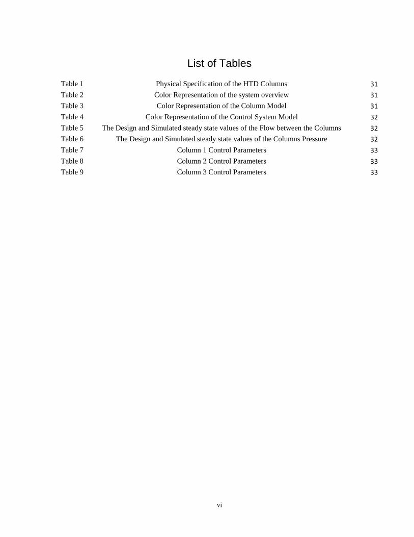
List of Tables

Table 1 Physical Specification of the HTD Columns 31

Table 2 Color Representation of the system overview 31

Table 3 Color Representation of the Column Model 31

Table 4 Color Representation of the Control System Model 32

Table 5 The Design and Simulated steady state values of the Flow between the Columns 32

Table 6 The Design and Simulated steady state values of the Columns Pressure 32

Table 7 Column 1 Control Parameters 33



vii

List of Figures

Figure 1 Block Diagram of DTRF Process 34

Figure 2 Tritium Removal Facility, Catalyst Exchange and Distillation 34

Figure 3 Tritium Removal Facility, Flow Diagram 35

Figure 4 High and Low Tritium Distillation Columns 36

Figure 5 Normal Packing Configuration 37

Figure 6 Packing Configuration during Flooding 38

Figure 7 Heater Control, Wiring Diagram 39

Figure 8 Node/Link Figure 40

Figure 9 Nodal Representation of a Column 40

Figure 10 A PID controller Block Diagram 41

Figure 10 B Cascade Controller Block diagram 41

Figure 11 System Overview 42

Figure 12 Single Entry of Warning Mechanism 43

Figure 13 Column Overview 44

Figure 14 Control System Overview 45

Figure 15 Condenser 1 Level, Plant Data, Feb 14, 2011 46

Figure 16 Condenser 1 Level, Condenser 1, HTD Model 46

Figure 17 Column 1 Apparent Level, Plant Data, Feb 14, 2011 46

Figure 18 Column 1 Apparent Level, HTD Model 46

Figure 19 Condenser 1 Level, Plant Data, Jan 01, 2011 47

Figure 20 Condenser 1 Level, Condenser 1, HTD Model 47

Figure 21 Column 1 Apparent Level, Plant Data, Jan 01, 2011 47


Figure 23 Column 2 Apparent Level, Plant Data, Jan 27, 2011 48


Figure 25 PID Controller, No Fault, Column 1 49

Figure 26 Proposed Cascade Controller, No Fault, Column 1 49

Figure 27 Optimized Cascade Controller, No Fault, Column 1 49

Figure 28 PID Controller, Heater Fault, Column 1 50

Figure 29 Proposed Cascade Controller, Heater Fault, Column 1 50

Figure 30 Cascade Controller, Heater Fault, Column 1 50

Figure 31 PID Controller, Power Transducer Fault, Column 1 51

Figure 32 Proposed Cascade Controller, Power Transducer Fault, Column 1 51

Figure 33 Optimized Cascade Controller, Power Transducer Fault, Column 1 51

Figure 34 PID Controller, Column 1 52

Figure 35 Proposed Cascade Controller, Column 1 52

Figure 36 Optimized Cascade Controller, Column 1 52

Figure 37 PID Controller, Column 2 53

viii

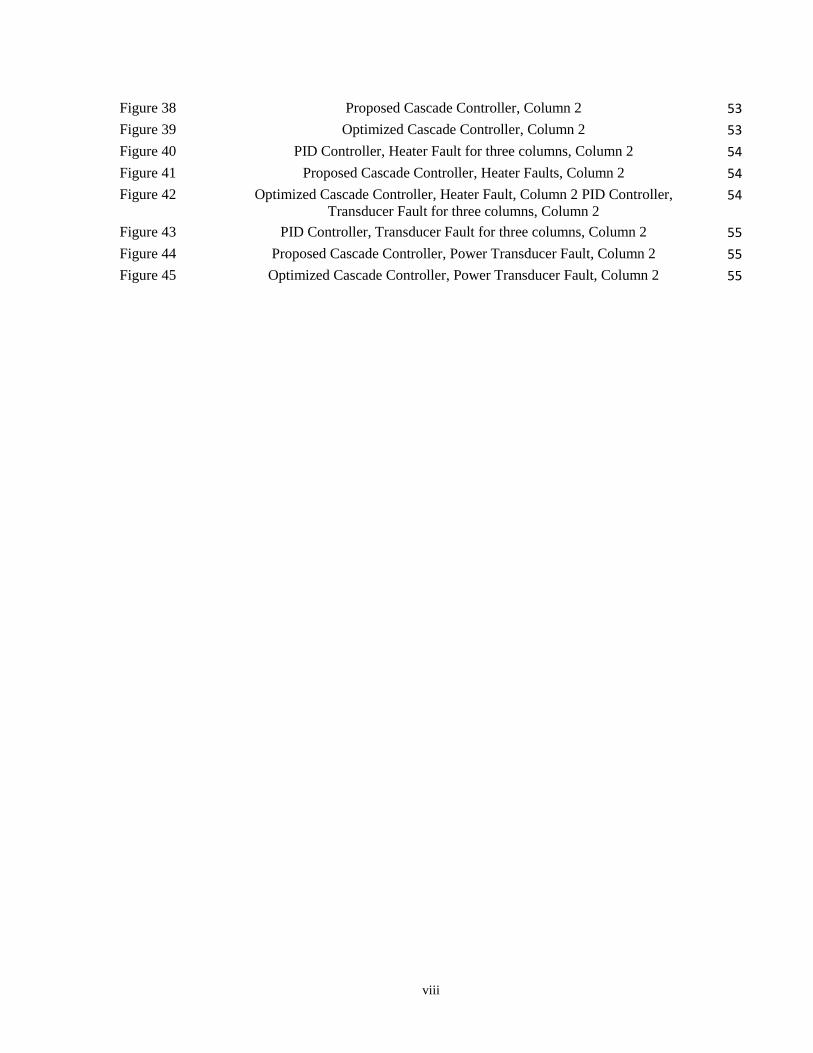
Figure 38 Proposed Cascade Controller, Column 2 53

Figure 39 Optimized Cascade Controller, Column 2 53

Figure 40 PID Controller, Heater Fault for three columns, Column 2 54

Figure 41 Proposed Cascade Controller, Heater Faults, Column 2 54

Figure 42 Optimized Cascade Controller, Heater Fault, Column 2 PID Controller,

Transducer Fault for three columns, Column 2 54

Figure 43 PID Controller, Transducer Fault for three columns, Column 2 55

Figure 44 Proposed Cascade Controller, Power Transducer Fault, Column 2 55

Figure 45 Optimized Cascade Controller, Power Transducer Fault, Column 2 55

ix

List of Appendices

Tables 31

Figures 34

x

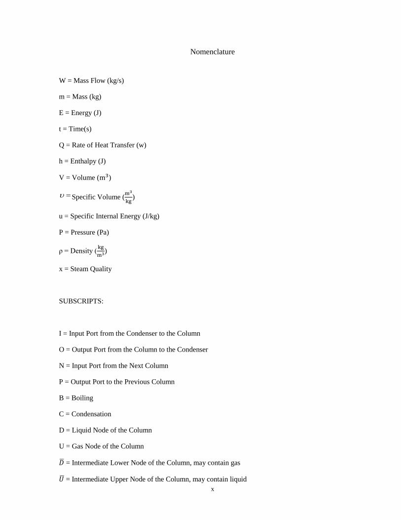
Nomenclature

W = Mass Flow (kg/s)

m = Mass (kg)

E = Energy (J)

t = Time(s)

Q = Rate of Heat Transfer (w)

h = Enthalpy (J)

V = Volume ( )

Specific Volume (

)

u = Specific Internal Energy (J/kg)

P = Pressure (Pa)

ρ = Density (

)

x = Steam Quality

SUBSCRIPTS:

I = Input Port from the Condenser to the Column

O = Output Port from the Column to the Condenser

N = Input Port from the Next Column

P = Output Port to the Previous Column

B = Boiling

C = Condensation

D = Liquid Node of the Column

U = Gas Node of the Column

= Intermediate Lower Node of the Column, may contain gas

= Intermediate Upper Node of the Column, may contain liquid

xi

T = Total Combination of the Column Nodes

sat = Saturation

l = liquid

g = gas

xii

Glossary

AU Adsorber Unit

CD Condensation

CRS Cryogenic Refrigeration System

DCS Distributed Control System

DMS Deuterium Make-UP System

DTRF Darlington Tritium Removal Facility

DU Dryer Unit

FTS Feed Treatment System

HTCB High Tritium Cold Box

HTD High Tritium Distillation

IMC Internal Model Control

LTCB Low Tritium Cold Box

LTD Low Tritium Distillation

OPG Ontario Power Generation

PID Proportional Integral Derivative

QDR Quarter Decay Ratio

RS Recombiner System

SCR Silicon Control Rectifier

TRF Tritium Removal Facility

TRIAC Triode for Alternating Current

VPCE Vapour Phase Catalytic Exchange

1

1. Introduction

1.1 Objectives

The objective of this study is to evaluate the effectiveness of the three different configurations

for the High Tritium Distillation (HTD) controller and assess their impact on the overall plant

performance. In particular, the current PID controller and two different cascade control

configurations are modeled and their effect on the apparent mismatch between the controller

output and the heater are evaluated.

1.2 Problem Statement

Darlington nuclear station has experience some undesirable behaviour in their HTD system due

to poor performance of the level controllers in the three columns of the Tritium Removal Facility

(TRF). Specifically, the sudden reduction of the column levels, level oscillations that happen

simultaneously and individually in sequence and also negative level indications are major

concerns. Furthermore, the electrical heaters which provide heat to the columns do not follow the

output of the controllers received as 4-20 mA signals. For example, the heater wattage appears to

be lower than expected in some cases and spikes are observed in the heater wattage.

2

2. System Description

2.1 Darlington Tritium Removal Facility

The Darlington TRF (DTRF) is operated by Ontario Power Generation (OPG) and is designed to

remove tritium from the heavy-water systems of all its CANDU reactor units. DTRF is capable

of processing 2.5 Gg of heavy-water annually and extract tritium with a purity >99%, at an

average tritium activity of 370 GBq/kg (10 Ci/kg ). The annual heavy-water-processing

rate corresponds to a tritium extraction rate of 2.5 kg( )/year. Unlike any other civilian tritium-

handling facility in the world, the DTRF functions very much like a production facility.

A schematic diagram of the DTRF process is shown in Figure 1 in Appendix B.

Tritium from heavy water is removed in two steps. In step 1, tritium from heavy water is

transferred to a gas stream using an eight-stage vapour-phase-catalytic-exchange (VPCE)

unit, and the detritiated heavy water is returned to service.

The system will reduce and maintain lower levels of tritium in the Nuclear Reactor Moderator

and Heat Transport Systems. This will result in lower radiation doses to operating personnel and

reduce the level of radiation in any releases of heavy water to the environment.

In step 2, the tritium-enriched stream from the VPCE is fed to a Condensation (CD) unit to

separate tritium from . A three-column system is used to separate tritium from . The purity of

the tritium product extracted is >99% .

In nuclear reactors the tritium is found in chemical combination with deuterium and oxygen in

the form of “tritiated heavy water”. The DTRF consists of a front-end composed of vapour phase

catalytic exchange and a back-end system consisting of cryogenic distillation. The tritiated heavy

water is contacted with a pure deuterium gas stream in the presence of a catalyst. This transfers

the tritium from the water to the deuterium gas (actually a mixture of the three hydrogen

isotopes, protium, deuterium and tritium). This gas is then distilled at cryogenic temperature to

separate the tritium (See Figure 2 in Appendix B).

3

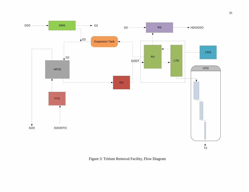
Figure 3 in Appendix B illustrates the TRF system and some of its major components such as:

Feed Treatment System (FTS), Vapour Phase Catalytic Exchange (VPCE), Dryer Unit (DU),

Adsorber Unit (AU), Low Tritium Distillation (LTD), High Tritium Distillation (HTD),

Cryogenic Refrigeration System (CRS), Recombiner System (RS) and Deuterium Make-Up

System (DMS)

Feed Treatment System (FTS):

The tritiated heavy water from the reactor is transferred to the TRF on a batch basis. From the

feed tanks a continuous flow is passed through a feed treatment system which eliminates

insoluble solids, gases and organic contaminants. This is done by passing the feed through a

degassing column, an evaporator and condenser, activated carbon adsorbers and filters.

Vapour Phase Catalytic Exchange (VPCE):

The feed then passes to the Vapour Phase Catalytic Exchange (VPCE) cascade. This is a

multistage counter current system with concurrent flow of heavy water vapour and deuterium gas

within each stage. Each stage consists of an evaporator, superheater, catalyst vessel and

condenser. The chemical reaction causing the transfer of tritium from heavy water to the

deuterium gas stream is:

DTO + ⇔ DT + (1)

The number of stages in the VPCE cascade is established by the required design detritiation

factor (the ratio of the tritium concentrations in the feed and return streams respectively). The

detritiated water flows to a product tank from which it is transferred back to the reactor systems

periodically.

Liquid ring compressors are used for compressing the deuterium gas which flows from the

VPCE to the Dryer Unit and for compressing the return gas from the distillation columns to the

VPCE. These were selected because could be used as the sealing and cooling liquid in the

compressors. This assured that contamination of the deuterium gas with oil or some other

compressor lubricant would not be a problem.

4

Dryer Unit (DU):

After leaving the VPCE cascade, the deuterium gas stream enriched with tritium is compressed

and passed through a regenerable dryer unit to remove the heavy water vapour carried over with

the gas.

Adsorber Unit (AU):

The dried gas enters a vacuum insulated cold box (the Low Tritium Cold Box); it is cooled and

passes through a cryogenic adsorber which extracts traces of nitrogen, oxygen and heavy water.

It is then further cooled down to almost the deuterium saturation temperature before entering the

low tritium distillation column.

Low Tritium Distillation (LTD):

The low tritium cold box contains a single column which enriches the less volatile tritium in the

bottom part. The bottom product from this column is transferred continuously to the high tritium

cold box.

The tritium depleted deuterium stream leaving the upper section of the low tritium distillation

column is recycled to the VPCE cascade.

High Tritium Cold Box (HTCB):

This cold box is equipped with three columns in series in which the tritium concentration

increases progressively. These columns are of successively smaller diameters to minimize the

inventory of tritium in the system. Tritium with an atomic purity of 99.9% is withdrawn from the

bottom of the last column and transferred to the Tritium Immobilization System.

Cryogenic Refrigeration System (CRS):

This system produces the refrigeration necessary for cooling down and continuous operation of

the columns. The hydrogen of the Cryogenic Refrigeration System is compressed by means of

Sulzer oil free labyrinth piston compressors. The compressed gas is then cooled in counter

current heat exchangers by transfer of sensible heat to the return stream. The low temperature

process configuration of the Cryogenic Refrigeration System is fairly complex, reflecting its dual

5

functions as a cooling system and as a heat pump operating between the low tritium column

reboiler and condenser. The refrigerant leaving the condenser warms up close to room

temperature in the counter current heat exchangers mentioned above and returns to the

compressor suction inlet.

Recombiner System (RS):

A Recombiner is provided to convert deuterium gas to water. This is required during

regeneration of the nitrogen adsorber, and also whenever the low tritium column is used to in its

secondary function of stripping protium from deuterium, in addition to being the first stage of the

tritium concentration process.

More importantly, the Recombiner is used to burn down the inventory of the LTD and HTD

systems prior to an outage during which maintenance is to be performed with these systems to be

opened to atmosphere.

The recombiner is a combustion type unit in which the hydrogen is burned via a diffusion flame

in a controlled atmosphere.

Deuterium Make-Up System (DMS):

A make-up electrolyzer is provided to produce the required inventory of deuterium for filling the

VPCE, LTD and HTD systems before startup and to compensate for the losses of hydrogen

isotopes from the system which result from protium extraction, adsorber regeneration and tritium

draw-offs. The electrolyzer splits heavy water into deuterium and oxygen. The deuterium is

admitted to the LTD/HTD/VPCE closed circulation loop and the oxygen can be utilized in the

recombiner.

2.2 High Tritium Distillation

The purpose of the high tritium distillation is to increase the /DT separation, convert

deuterium-tritide to deuterium and tritium, and to achieve a bottom concentration which contains

tritium with not more than 0.001 atomic fraction of deuterium and protium.

Figure 4 in Appendix B illustrates the schematic of the HTD and its major components.

6

The necessary reflux for the columns is drawn from the reboilers as vapour by the corresponding

condensers. The slightly higher pressure in the subsequent column, which is necessary to

compensate for the pressure drop of the interconnecting transfer lines, is provided by the static

head of liquid in a hydraulic sealing siphon.

The conversion of deuterium-tritide to deuterium and tritium takes place in a catalyst converter

which operates at ambient temperature. The catalyst was originally supplied as Platinum on

Charcoal, i.e., similar to the VPCE catalyst. However, during initial operation, blockage was

experienced in the HTD process systems. A possible cause of this blockage was attributed to the

formation of methane by the radiolytic action of tritium on charcoal, with the resultant freezing

out. The catalyst was changed to platinum on alumina, and since then, blockage of the HTD

process systems has not been experienced. A vacuum unit is provided to evacuate HTD. The

exhaust gases pass an oil mist eliminator. They are collected in an exhaust holding tank.1

Total reflux is the mode used for start up. Twenty-four hours after start up the tank is already

purged five times thus recalculating at least 99% of the tritium inventory.

The design of the separation cascade is optimized with respect to hold-up, Curie inventory, DT

conversion, packing efficiency and column manufacture. This leads to a three fold cascade.

The physical specification of the three columns is listed in table 1 in Appendix A.

All columns are controlled in the same way: The heating power to the reboiler is controlled by a

level controller. The reflux rate is controlled by the level of the liquid hydrogen in the head

condenser. This level is adjusted according to the power consumption of the relevant reboiler

heating elements. During total reflux, the pressure controller is hooked up to the level controller

of condenser 1. In normal operation, the pressure is controlled by the pressure of the LTD

column.

1 The contents of the exhaust holding tank may be directed to the Ail Cleanup System (if the hydrogen isotope

concentration is high enough) or directly up the stack (if the hydrogen concentration is low).

7

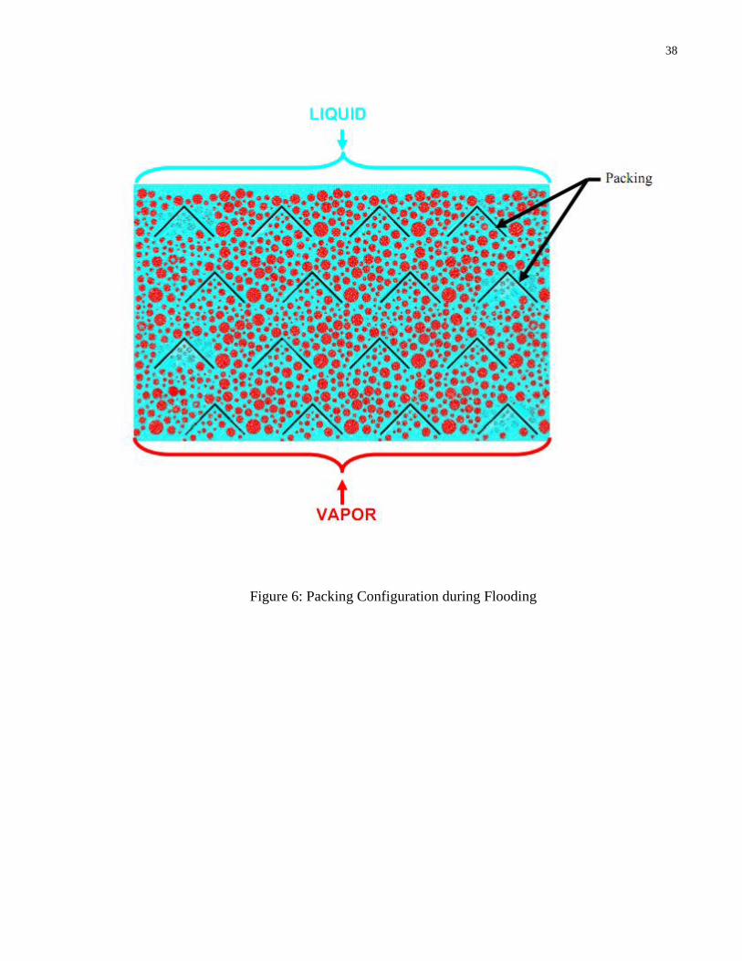
2.2.1 Flooding Event

Flooding in distillation columns has been defined as excessive accumulation of liquid inside the

column or inoperability due to excessive retention of liquid inside the column and even a point

where it is difficult to obtain net downward flow of liquid, and any liquid fed to the column is

carried out with the overhead gas. While these descriptions appear to be similar at first glance,

they actually describe different stages or degrees of flooding. Excessive accumulation of liquid

may or may not cause inoperability, and inoperability may or may not carry the feed liquid out

with the overhead gas.

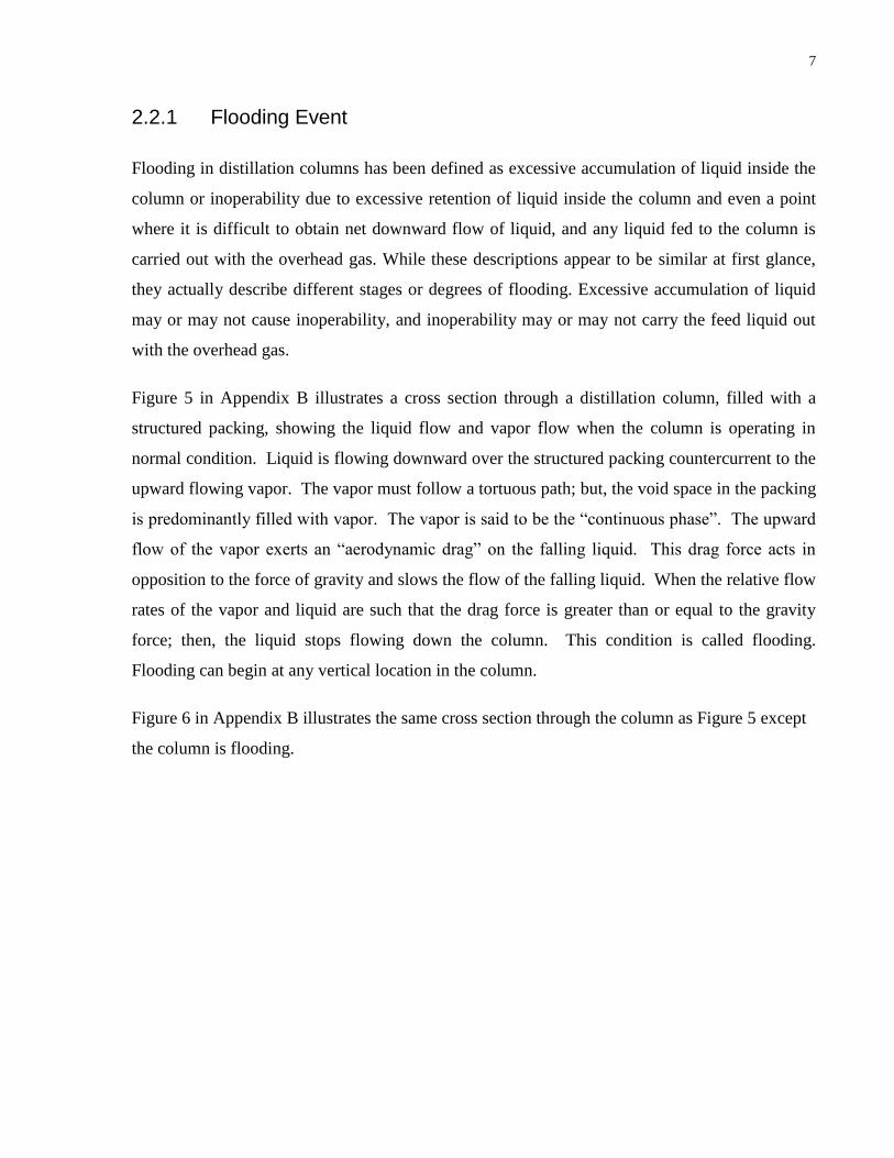
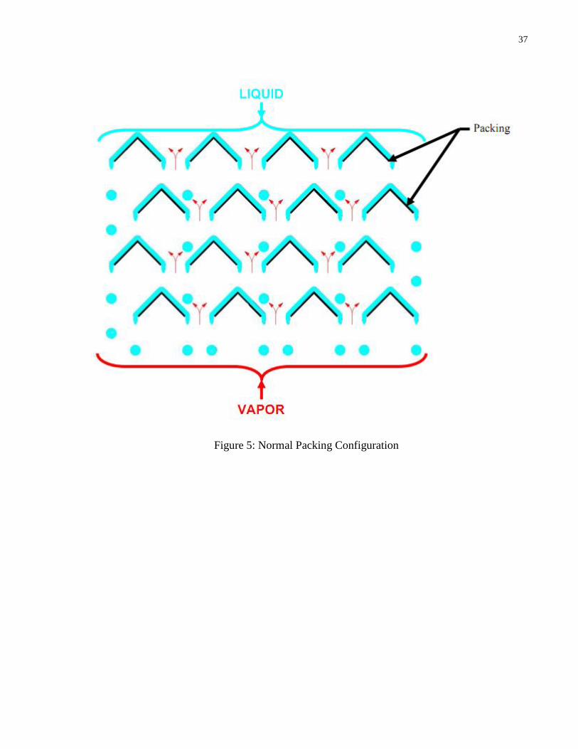
Figure 5 in Appendix B illustrates a cross section through a distillation column, filled with a

structured packing, showing the liquid flow and vapor flow when the column is operating in

normal condition. Liquid is flowing downward over the structured packing countercurrent to the

upward flowing vapor. The vapor must follow a tortuous path; but, the void space in the packing

is predominantly filled with vapor. The vapor is said to be the “continuous phase”. The upward

flow of the vapor exerts an “aerodynamic drag” on the falling liquid. This drag force acts in

opposition to the force of gravity and slows the flow of the falling liquid. When the relative flow

rates of the vapor and liquid are such that the drag force is greater than or equal to the gravity

force; then, the liquid stops flowing down the column. This condition is called flooding.

Flooding can begin at any vertical location in the column.

Figure 6 in Appendix B illustrates the same cross section through the column as Figure 5 except

the column is flooding.

8

3. HTD Control

3.1 General

The tritium/deuterium mixture enters the High Tritium Cold Box (HTCB) through a motorized

valve and flows into the Condenser 1 where it is condensed using liquid hydrogen as a coolant

(See Figure 4).

From the Condenser 1, it flows through the first column, Column 1, into the bottom evaporator

in the column where it is evaporated. The condenser level is controlled on the hydrogen side of

Low Tritium Cold Box (LTCB); the evaporator level is also controlled.

The level control is achieved by varying the power that is generated by an electrical heater.

Part of the evaporated deuterium is directed to the second column, Column 2, where it is treated

exactly in the same way as in column 1. From column 2, the deuterium flows to the third

column, column 3, and is treated once again in the same way.

The deuterium/tritium mixture which is leaving column 3 passes through heat exchanger 2 to be

warmed up for the conversion reaction 2DT → which takes place in the catalytic

converter.

The return stream from catalytic converter is passing through heat exchanger 2 to be cooled

down again, before it is fed into the column 2.

The deuterium leaves the HTCB coming from column 1 through a motorized valve.

The HTCB is kept under high vacuum by the diffusion pumps and the roughing pumps. The

exhaust (tritium containing) gases are collected in a tank.

The helium extraction motorized valves and the total reflux motorized valve are closed during

this operation.

9

3.2 Measurements

The reboiler levels are measured indirectly using the aluminum block temperature; the lower the

temperature of the aluminum block, the higher is the level. Two different physical effects are

used to get a redundant measure:

1. Vapour pressure of neon (P-transmitter)

2. Electrical resistance (Diode)

The two signals are compared and the lower temperature is used for control in the Level

Indicating Controller.

Since the level of the columns is not directly measured and is implied from the temperature of

the column, this measurement will be called Apparent Level from here on.

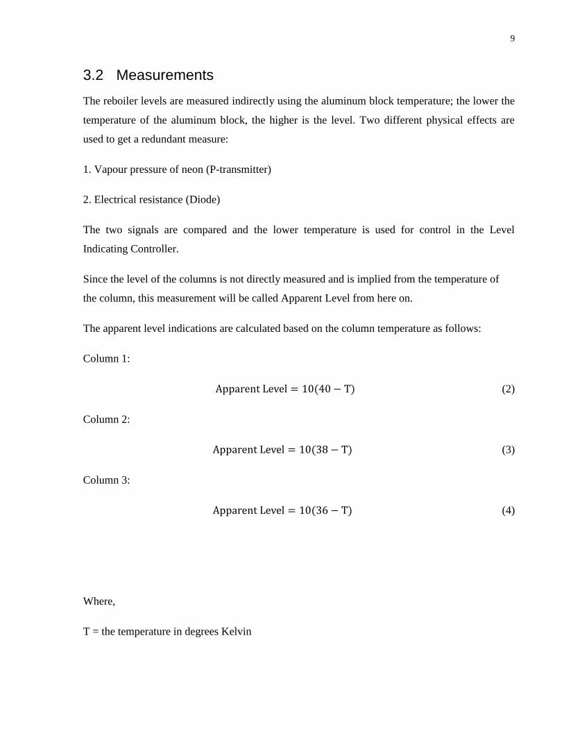
The apparent level indications are calculated based on the column temperature as follows:

Column 1:

(2)

Column 2:

(3)

Column 3:

(4)

Where,

T = the temperature in degrees Kelvin

10

Each column has a variable electrical heater connected to the bottom. The electrical heaters are

placed in aluminum casings.

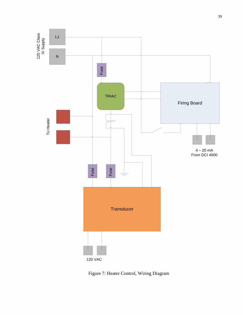
3.3 Heater Control

The heater controller is the primary control mechanism controlling the level of each column.

When it is required to reduce the level of a column, the heater associated with that column will

be automatically turned up by the controller to provide more heat to increase the boiling within

the column. When it is required to increase the column level, the heater will be automatically

turned down. The control signal from the heater controller, in the form of 4-20 mA signal, is fed

to the firing board. The firing board is a Silicon controlled Rectifier (SCR). The modulated pulse

generated from the firing board is received by the Triode for Alternating Current (TRIAC) which

in turn regulates the amount of current passing through the TRIAC from the power supply to the

heater. The output of the TRIAC is also received by the Transducer for power measurement (See

Figure 7 in Appendix B).

4. Mathematical HTD Model

This section describes the details of the HTD mathematical model which is used to simulate the

HTD transients.

4.1 Assumptions and Limitations

The following assumptions are made for the HTD model:

1. The reflux flow from a column to the previous column is compressible turbulent gas flow.

2. The Catalytic Converter acts only as a part of the pressure drop of the Column 3 reflux to Column

2.

3. The temperature of deuterium entering Heat Exchanger 2 and leaving Catalytic Converter are

assumed to be the same based on the design manual.

4. The flow through the internal reflux line that brings the reflux flow back to the column is

negligible.

5. The fluid temperature change due to passing through the extension to the cold box, located in top

right side of the cold box, is negligible.

6. The pressure listed in the design manual for the low tritium column can be used for the portion of

the column connected to HTD.

7. The feed concentration is 10 Ci/kg .

11

8. The flow through the Heat Exchanger 1 and expansion tank are ignored in this model. Based on

the design manual this flow is very small and it is only 1.64% of the total flow exiting column 1

of HTD.

9. The enthalpy drop in the pipes connecting the columns is negligible and ignored.

10. The change of deuterium density due to change in pressure within one time step of the simulation

is assumed to be negligible.

11. Deuterium and Tritium are assumed to be ideal gases.

Limitation:

Due to the unavailability of the manufacturer’s data for some of the components, the information

from the most similar component from the same manufacturer was used.

4.2 Hydraulic Network Theory

The purpose of the hydraulic network model is to predict the transient behaviour of the HTD

during normal operation. This requires solving the mass and energy balances for a single fluid,

one-phase, one dimensional flow. The implementation of these equations for a generic hydraulic

network is described. Specific configurations for HTD system can then be developed using the

techniques described for the generic model as a basis.

The phenomena to be modelled that shall be validated include:

Single fluid, one phase, one dimensional pressure flow dynamics including

pressure characteristics, pressure losses due to friction, gravity pressure and fittings.

Convective heat transport phenomena for the fluid as it travels through the

network and exchanges heat with the heat exchangers.

Thermodynamic properties of deuterium and tritium. In general, deuterium and

tritium properties are required for the sub-cooled liquid region, and the saturated

region.

12

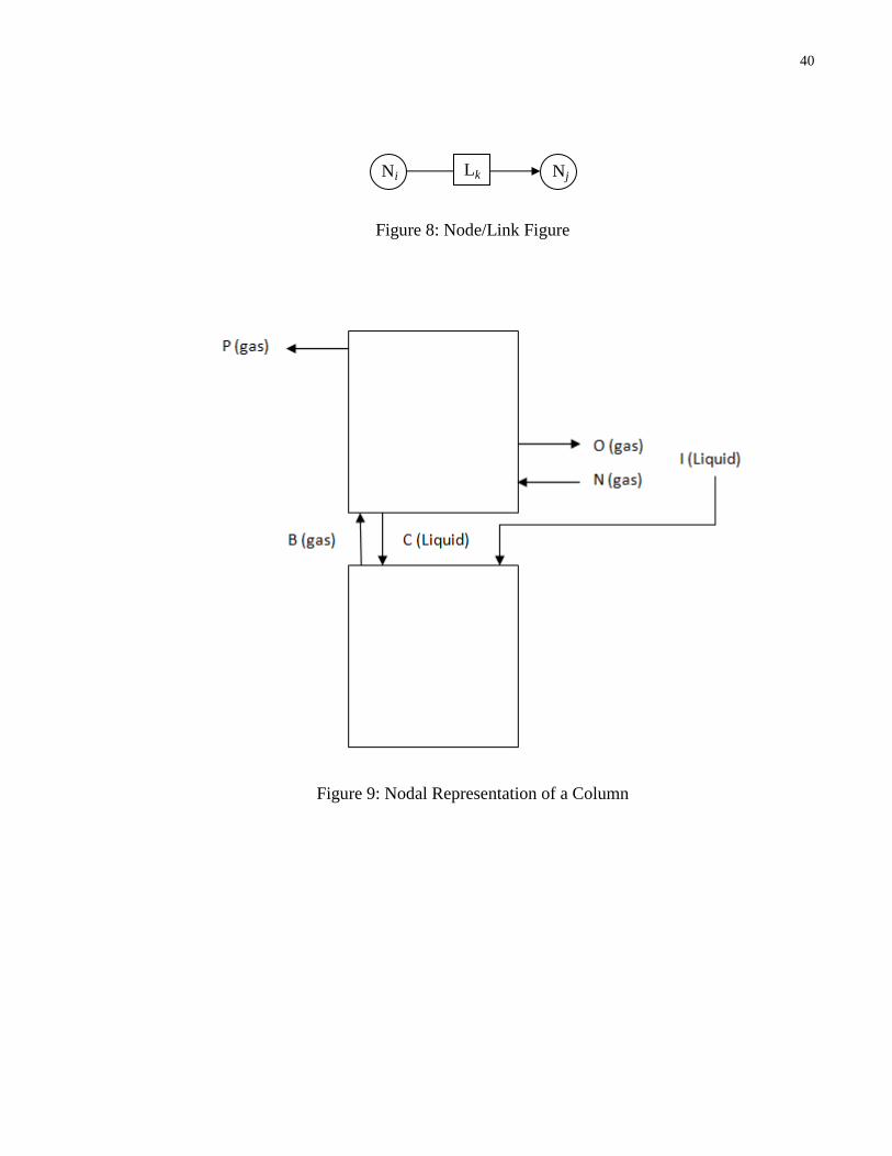
4.2.1 The Hydrodynamic Network Model

The physical flow network system is represented by nodes and links. Figure 8 in appendix B

shows a block presentation of a node and its links.

The link Lk is assigned node Ni as its initial node and Nj as its terminal node. There are two

kinds of flow paths. The normal circuit fluid flow passages are termed as the “noncritical link”

from which no leakage is considered to take place. Therefore, the flow is governed by a one-

dimensional momentum balance equation of the form

(5)

Where,

Wk = mass flow (kg/s)

pi, pj = pressures at the initial and terminal nodes respectively (Pa)

t = time (s)

Fk = a general nonlinear function

A node i may be associated with a finite number of links which either initiate from or terminate

at i. Conditions of the node are governed by the mass and energy conservation equations.

4.2.2 Basic Equations

Mass balance:

(6)

13

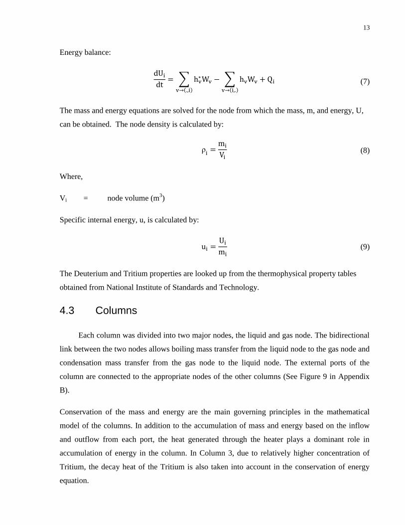
Energy balance:

(7)

The mass and energy equations are solved for the node from which the mass, m, and energy, U,

can be obtained. The node density is calculated by:

ρ

(8)

Where,

Vi = node volume (m3)

Specific internal energy, u, is calculated by:

(9)

The Deuterium and Tritium properties are looked up from the thermophysical property tables

obtained from National Institute of Standards and Technology.

4.3 Columns

Each column was divided into two major nodes, the liquid and gas node. The bidirectional

link between the two nodes allows boiling mass transfer from the liquid node to the gas node and

condensation mass transfer from the gas node to the liquid node. The external ports of the

column are connected to the appropriate nodes of the other columns (See Figure 9 in Appendix

B).

Conservation of the mass and energy are the main governing principles in the mathematical

model of the columns. In addition to the accumulation of mass and energy based on the inflow

and outflow from each port, the heat generated through the heater plays a dominant role in

accumulation of energy in the column. In Column 3, due to relatively higher concentration of

Tritium, the decay heat of the Tritium is also taken into account in the conservation of energy

equation.

14

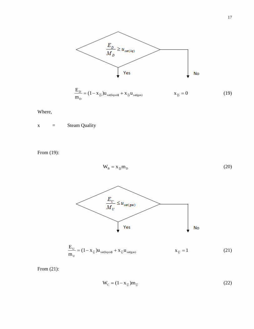
The amount of vaporization and condensation is determined by comparing the specific internal

energy of the node with the saturation internal energy corresponding to the calculated pressure of

that instance in time. Any excess energy contained in the liquid node is converted to gas through

boiling while the lack of energy in the gas node is compensated through condensation (See

Equations 21-24).

In this approach, the change of deuterium density due to change in pressure within one time step

of the simulation is assumed to be negligible. Therefore, the approximated volume of the liquid

node will be used to calculate the volume of the gas node. Solving the conservation of mass and

energy equations, the specific volume and specific internal energy are also calculated. With

either of the two properties, the new pressure of the gas node can be calculated.

The nodal configuration does not necessary agree with the geometric setup of the column. For

instance, the liquid entering from the top of the column, in this case, will be directly entering the

bottom node which is the liquid node. This does not affect the dynamics of the model as it is

used only as a geometric convention.

Figure 9 represents a nodalized configuration of a single column. The symbols used for each

node or link are used as subscripts in the equations2.

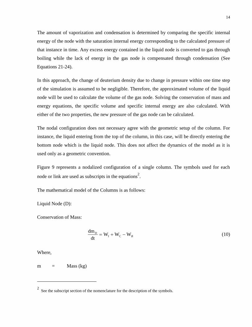
The mathematical model of the Columns is as follows:

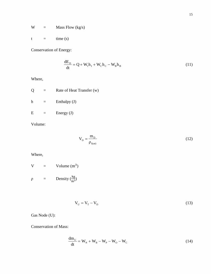
Liquid Node (D):

Conservation of Mass:

BWWWdt

dmCI

D (10)

Where,

m = Mass (kg)

2 See the subscript section of the nomenclature for the description of the symbols.

15

W = Mass Flow (kg/s)

t = time (s)

Conservation of Energy:

BBCCIID hWhWhWQ

dt

dE (11)

Where,

Q = Rate of Heat Transfer (w)

h = Enthalpy (J)

E = Energy (J)

Volume:

l(sat)

DD

ρ

mV (12)

Where,

V = Volume ( )

ρ = Density (

)

DTU VVV (13)

Gas Node (U):

Conservation of Mass:

COPBNU WWWWW

dt

dm (14)

16

Conservation of Energy:

CCOOPPBBNNU hWhWhWhWhW

dt

dE (15)

From (14), (13):

U

U

Um

Vυ (16)

Where,

= Specific Volume (

)

From (15), (14):

U

U

Um

Eu (17)

Where,

u = Specific Internal Energy (J/kg)

We assume:

UD PP (18)

Where,

P = Pressure (Pa)

17

sat(gas)D)sat(liquidD

D

D ux)ux(1m

E 0x

D (19)

Where,

x = Steam Quality

From (19):

DDB mxW (20)

sat(gas)U)sat(liquidU

U

U ux)ux(1m

E 1x

U (21)

From (21):

UUC )mx(1W (22)

18

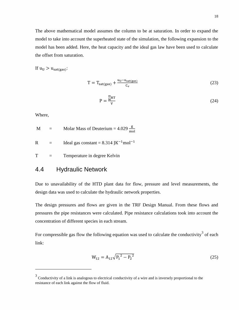
The above mathematical model assumes the column to be at saturation. In order to expand the

model to take into account the superheated state of the simulation, the following expansion to the

model has been added. Here, the heat capacity and the ideal gas law have been used to calculate

the offset from saturation.

If :

(23)

(24)

Where,

M = Molar Mass of Deuterium = 4.029

R = Ideal gas constant = 8.314

T = Temperature in degree Kelvin

4.4 Hydraulic Network

Due to unavailability of the HTD plant data for flow, pressure and level measurements, the

design data was used to calculate the hydraulic network properties.

The design pressures and flows are given in the TRF Design Manual. From these flows and

pressures the pipe resistances were calculated. Pipe resistance calculations took into account the

concentration of different species in each stream.

For compressible gas flow the following equation was used to calculate the conductivity3 of each

link:

(25)

3 Conductivity of a link is analogous to electrical conductivity of a wire and is inversely proportional to the

resistance of each link against the flow of fluid.

19

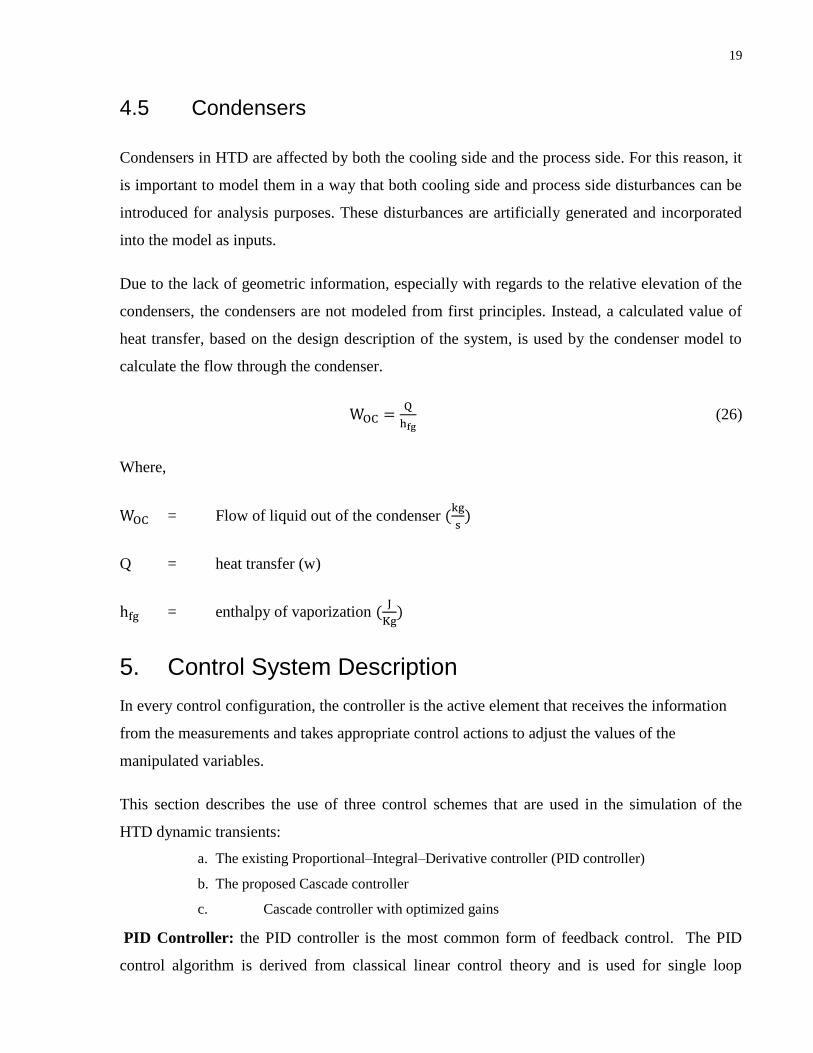
4.5 Condensers

Condensers in HTD are affected by both the cooling side and the process side. For this reason, it

is important to model them in a way that both cooling side and process side disturbances can be

introduced for analysis purposes. These disturbances are artificially generated and incorporated

into the model as inputs.

Due to the lack of geometric information, especially with regards to the relative elevation of the

condensers, the condensers are not modeled from first principles. Instead, a calculated value of

heat transfer, based on the design description of the system, is used by the condenser model to

calculate the flow through the condenser.

(26)

Where,

= Flow of liquid out of the condenser

Q = heat transfer (w)

= enthalpy of vaporization

5. Control System Description

In every control configuration, the controller is the active element that receives the information

from the measurements and takes appropriate control actions to adjust the values of the

manipulated variables.

This section describes the use of three control schemes that are used in the simulation of the

HTD dynamic transients:

a. The existing Proportional–Integral–Derivative controller (PID controller)

b. The proposed Cascade controller

c. Cascade controller with optimized gains

PID Controller: the PID controller is the most common form of feedback control. The PID

control algorithm is derived from classical linear control theory and is used for single loop

20

systems. The PID algorithm consists of three basic modes, the proportional, the integral and the

derivative modes.

Digital controllers are often synthesized by approximating continuous controllers. The discretized PID

controller using a simple approximation resulting in:

Where,

= control signal at sample time k

= Initial Value of the Control Signal

= Controller Gain

= Integral Time (s)

= Derivative time (s)

= Sampling Interval (s)

= Control Error (e = r-y), r is the reference variable, y is the process measured

variable

It must be noted that the integral term does not have to be calculated for all k since a running

sum can be made and updated when the new error is calculated.

The integral, proportional and derivative parts can be interpreted as control actions based on the past, the

present and the future. The derivative part can also be interpreted as prediction by linear extrapolation.

Figure 10A in Appendix B illustrates a block diagram of a simple feedback loop governed by a PID

controller.

The existing Controller implemented in the HTD system is a PID controller. This controller is

modeled based on the manufacturer’s manual of the Distributed Control System (DCS) along

with the current operating control parameters. The existing controller is a discrete PID controller.

21

Cascade Controller: When a single-loop control does not provide acceptable control

performance, an enhancement such as cascade control is used. Cascade control strategy

combines two feedback controllers, with the primary controller’s output serving as the secondary

controller’s setpoint.

Figure 10B in Appendix B illustrates a schematic of a closed loop control system governed by a

cascaded controller.

In this study, the Proposed Cascade Controller is modeled based on the similar cascade controller

scheme proposed for HTD based on the requirements provided by TRF Operations Group4 as

well as the proposed controller parameters. The power measurement of the column heater and

the column temperature are the variables to be controlled by the inner loop and outer loop,

respectively.

Cascade controller with optimized inner loop control gain parameters: similar configuration

for the cascade controller described above is used with an exception of using a higher value for

the inner loop proportional gain to make the system response faster. This configuration is called

Optimized Cascade controller from here on.

The parameters of the outer loop PID controller were calculated using the Ziegler-Nichols

Quarter Decay Ratio (QDR) method. Since these values were very close to the existing PID

controller parameters, they were not modified in the model. The Internal Model Control (IMC)

method was used to calculate the parameters for the inner loops. In selecting the appropriate gain

values for the inner loop control parameters, special attention was made to make sure the system

remains stable at all time specially in the presence of unwanted disturbances.

The control parameters are listed in the Appendix A.

4 Unregistered document provided by Operations

22

6. Implementation and Validation of the Model

6.1 Process Model Implementation

The TRF HTD model is built on the MATLAB/SIMULINK simulation package. MATLAB is a

C based text structure programming language and SIMULINK is a graphic programming

language and provides blocks that may be combined to create "subsystems" or "modules".

The TRF HTD model development process (i.e. life-cycle) involves the use of modularity and

encapsulation. Each module is developed and tested independently. Modules are integrated to

form the overall TRF HTD model. This approach provides flexibility, process discipline,

consistency, and reusability of the developed codes.

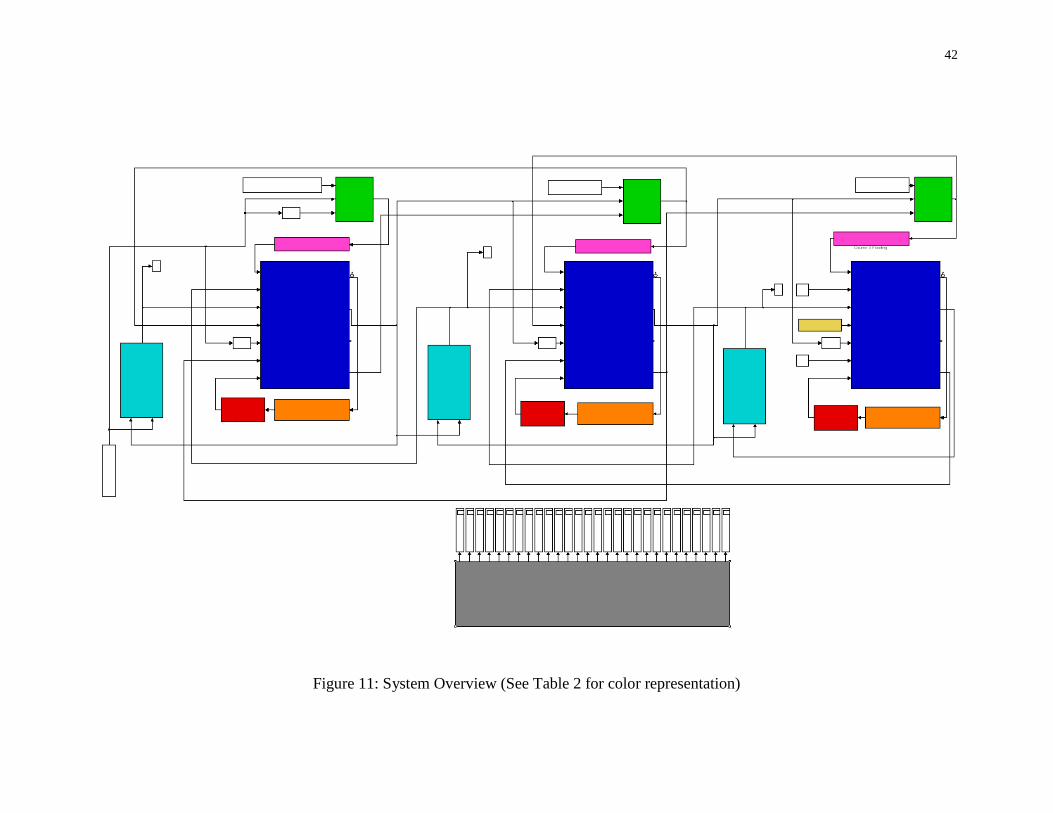
The major HTD components are modeled within a high level subsystem visible on the system

overview. Each component is placed in the system overview such that the configuration of the

model resembles a flow diagram. The components are placed in their appropriate locations both

with respect to the actual geometry of the plant and based on the flow diagram. (See Figure 11 in

Appendix B)

In order to validate the accuracy of the models, the parameters values are checked for several

different transients. In the validation process, the simulation results were also examined against

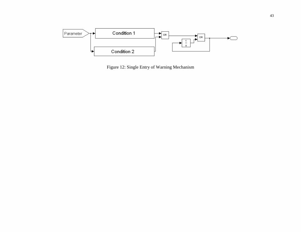
the assumptions listed in Section 3.1. A warning mechanism is developed to identify and report

any violation of those assumptions. Each entry of the warning mechanism checks a condition

under which one of the assumptions is valid. Physical boundaries of the system are also checked.

Furthermore, in this warning mechanism if a single condition is violated then a flag will be

raised and maintains its value until the end of the simulation. An additional entry has also been

added that checks all the other entries and flags the existence of at least one warning in the

system.

A single entry of the warning mechanism has been shown in Figure 12 in Appendix B.

In order to expand the model to take into account the column dry out, a dry out mechanism has

also been added to the column model. The column dry out mechanism is activated once the heat

supplied from the heater is exactly enough or exceeds the amount of heat needed to vaporize the

23

liquid inventory of the column plus the inflow of the liquid from the condenser. In this condition,

the excessive heat is directly applied to the gas node.

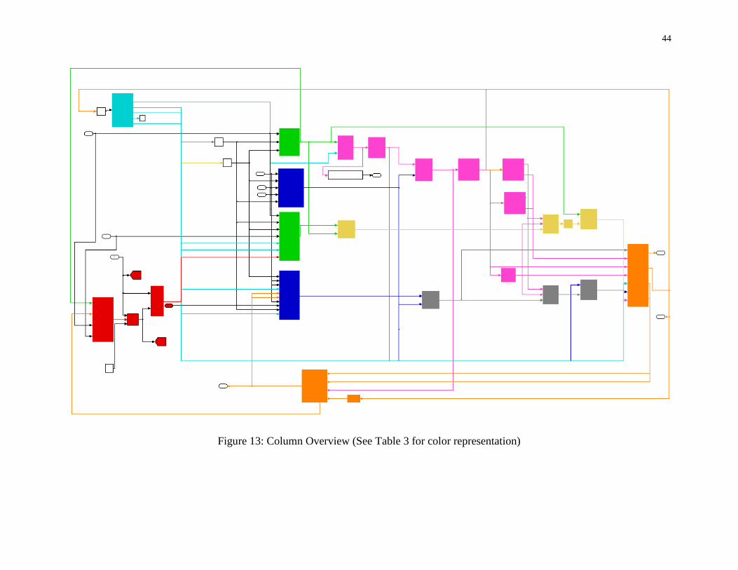
An overview of the column model is provided in Figure 13 in Appendix B. The colors of Table 3

in Appendix A present the major elements of the column model.

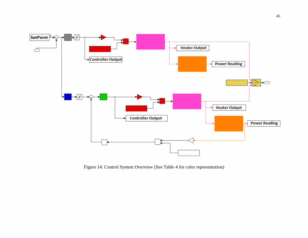
6.2 Control Model Implementation

A switch is used to select the desired control types. The selected control type will be flagged in

the initialization process.

Figure 14 in Appendix B shows an overview of the control system model. Table 4 in Appendix

A lists the colors presenting the major elements of the control system.

6.3 Validation of the Steady State Results

The accuracy of the HTD model developed in this study was validated by:

a. Comparing the steady-state response of the model vs. the design data from the design

manual. Specifically, the absolute values of the flows between the columns and the pressures

of each column were compared to design manual values

b. Comparing various transient responses to the real data collected during normal HTD

operation.

However, there were two challenges to validation of the HTD model:

1. There was significant deviation between some plant and design data.

2. There was limited plant data.

Table 5 and Table 6 in Appendix A provide a summary of the design and simulated steady-state

values for the column pressure and the flow between the columns for the feed concentration of

10 Ci/kg

6.4 Validation of the Transient Results

As the second stage of validation, external disturbances through the cooling side of condensers

and through the LTD are introduced to the HTD system and the shape of the trend is validated

against plant data. The disturbances added to the system model are selected from actual plant

data occurrences.

24

Condenser Level Step up:

A step increase in the condenser level is introduced and the resultant change in column level is

compared to a similar plant transient.

For the purpose of the following transient validations, it was assumed that the rate of heat

transfer in the condensers is linearly related to the level of coolant in each condenser.

The plant data for the column exhibits a faster response to the change in condenser level in

comparison with the simulated response. For visibility purposes, the time scale associated with

the simulated response is selected to be relatively shorter. (See Figures 15-18 in Appendix B)

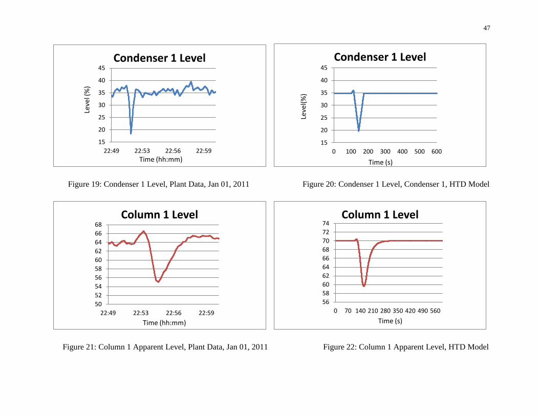
Condenser Level Dip:

A rapid decrease in condenser level is introduced and the resultant change in column level is

compared to a similar station transient. (See Figures 19-22 in Appendix B)

Column Flooding:

Distillation columns have known issues with moisture hold up and flooding. Due to the complex

nature of this phenomenon, it is not modeled from first principles. The plant data trend is

modeled as an artificial liquid build up within the column and the subsequent release. The same

disturbance observed in plant apparent level is reproduced. (See Figures 23 and 24 in Appendix

B)

7. Discussion of the Results

This section introduces three control logic configurations and assesses their effectiveness to

improve the dynamic responses of the HTD system to various operating conditions. The

transients that are examined include normal condition when there is no fault in the system and

also when system is subjected to fault in the heater and power transducer.

The plant data did not provide enough information to identify the failure of set point tracking of

the heater. This could be due to the fact that the heater response was only captured through the

power transducer reading. The fault magnitude was too small to have a discernible impact on the

25

temperature. It could not be determined whether the fault originates in the heater, the firing

board, the TRIAC or the power transducer. Thus, two different failure cases were examined.

a. The failure was assumed and modelled in the firing board and TRIAC systems. This

fault is called Heater Fault from here on.

b. The failure was assumed to be due to the power transducer measurement. This fault is

called Power Transducer Fault from here on.

One of the most dominant transients known to be experienced by distillation columns is a liquid

hold up phenomenon called Flooding. The effect of this phenomenon has also been captured by

the model such that it matches the plant data.

Condenser Level Step up:

This transient is the same as the one explained in Section 5.4. The condenser level step up

increases the amount of condensation in the condenser. This causes an increase in the liquid

inflow to the column. The raise of liquid inflow to the column reduces the temperature of the

column. As explained in Section 2.2, the lower the temperature of the aluminum block, the

higher is the apparent level calculated from column temperature.

Figures 25 to 27 in Appendix B show the condenser level step response transient for fault free

system using the existing controller, the proposed cascade controller, and the optimized cascade

controller. Evidently, the responses are almost identical.

Note that the Apparent Level for all column levels is dimensionless. Apparent level is derived

from temperature and is an estimation of the level trend not the absolute level value.

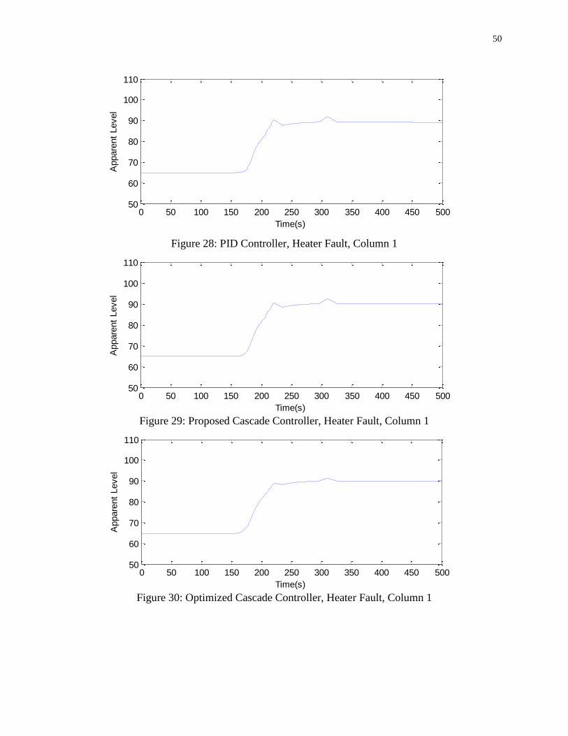
Figure 28 shows the PID Controller with a heater fault which affects the overall temperature of

the column. Hence, the effect of the fault is seen in the apparent level which is based on

temperature. Figures 29 and 30 show a similar transient for the proposed and optimized cascade

controllers. In principle, the cascade controller should have a favourable response to a heater

fault since the heater fault is detected before the temperature disturbance. However, the inner

loop gain in the proposed cascade controller is too small to make a visible difference. In Figure

30, due to higher inner loop gain, this difference is more visible.

Figure 31 shows that since the PID Controller does not use the power transducer measurement, it

is not affected by the fault. Figure 32 and 33 illustrates that in contrast to the PID Controller, the

26

fault in power transducer affects the control system and consequently the apparent level. The

optimized cascade controller, due to higher gain on the inner loop, experiences more of this

adverse effect.

The relative magnitudes of the faults and the transients are obtained from plant data. The effect

of the condenser transient is much larger than any of the introduced faults.

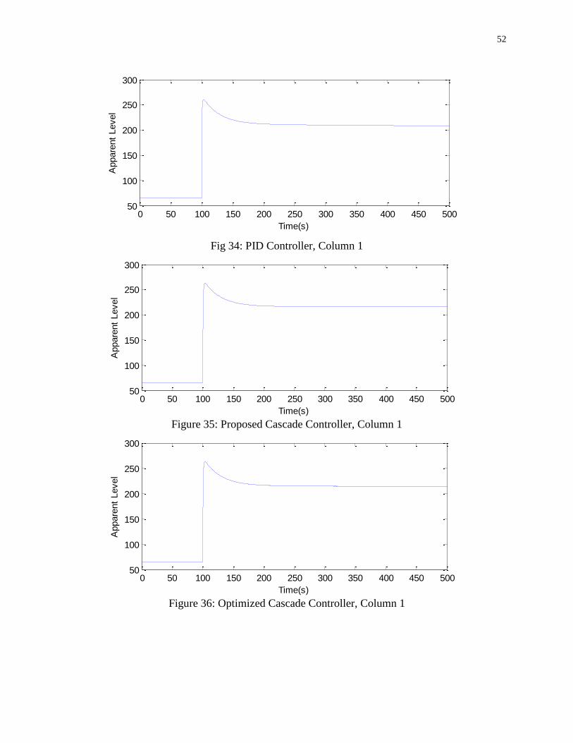
LTD Pressure Drop:

LTD pressure is stable. However, in order to analyze the new control, it is necessary to study the

effects of various disturbances including the ones that are not common. For this purpose, a

sudden pressure drop is introduced in the LTD and the response of HTD is shown. The

introduced pressure drop in LTD causes an increased pressure difference between LTD Column

and HTD Column 1. This increased pressure drop raises the flow from HTD Column 1 to LTD

Column. The increase in the outflow from HTD column 1 decreases the pressure and

temperature of Column 1. This is shown as an increase in the calculated apparent level.

The level of column 1 is shown since it has the most immediate and largest response to an LTD

pressure change.

Figure 34 in Appendix B shows the response of the apparent level in Column 1 as the closest

HTD column to LTD. The responses in Figures 35 and 36 are very similar to the ones in Figure

34.

Column Flooding:

This transient is the same as the one explained in Section 5.4. The column flooding starts by a

gradual liquid build up in the packing of the column. This liquid build up causes the bottom of

the column, where the temperature transducer is placed, to temporarily dry up increasing its

temperature. This is followed by a sudden release of the liquid originally trapped in the packing.

The liquid release will abruptly decrease the temperature returning the temperature to its original

value. The calculated apparent level shows a gradual decease followed by a sudden increase.

27

Figure 37 illustrates the response of the apparent level in Column 2 when the column goes

through flooding. The responses in Figures 38 and 39 are very similar to the response in Figure

37.

Multiple Faults:

To better understand the effect of the faults in the system heater faults were introduced at steady

state. The faults are introduced to all three columns simultaneously and their magnitudes were

increased for better visibility. The results are shown in Figures 40 to 45 in Appendix B.

Figure 40 shows a heater fault introduced in column 2 as well as the cascading effect of both

adjacent columns 1 and 3. Column 2 was selected in this case so that the cascading effect of fault

on each side of it can be included. Figures 41 and 42 show similar trends. However, Figure 42,

due to higher inner loop gain, shows a more favourable response to the disturbance as the

magnitude of the disturbance has reduced by about 28%. In Figure 43 it can be seen that the PID

Controller, having no input from the power transducer, is not prone to transducer faults. Figure

44 and 45 show the effect of transducer fault in the proposed and optimized cascade controllers.

Since the power transducer measurement is used in the inner loop of the cascade controller, its

fault affects the overall control of the apparent level. In contrast to the heater fault, Figure 45

shows a more unfavourable response due to higher inner loop gain.

8. Conclusions

The assessment in this thesis investigated the effectiveness of three control configurations to

improve the performance of the HTD system. Different system transients were simulated when

there was no fault in the system and when system was subjected to some faults.

The simulation results show that all three control schemes produce similar responses.

The cause of the apparent mismatch between the controller output and the power transducer

reading is unknown. This could be due to a fault in the components leading to the heater (Firing

board or TRIAC), a fault in the power transducer or it could be an artefact of the data due to

sampling.

28

In case of a fault in the firing board or TRIAC fault, the system response under a cascade

controller shows a slight improvement5.

However, if the fault originates from the power transducer, the cascade control will create an

adverse effect which is not present in the current control scheme. This is due to the fact that the

fault introduced is present in the inner loop of the cascade controller where the PID Controller

does not have this loop. In the PID Controller the power transducer output is not used and hence

the PID Controller is not affected by the power transducer fault.

Both the simulation results and the plant data indicate that the impact of the heater versus

controller mismatch, whatever the cause may be, is negligible (e.g. Figures 28-33).

It is not clear what impact the inner loop would have on the heater integrity if the column went

dry. The heater resistance should increase when the liquid cooling is removed. This will

increase the resistance and decreases the power input to the heater. At some point the heater

input and output will balance. With the present architecture, the heater power is measured but

not controlled so the control system does not increase the demanded heater power to compensate

for the increased resistance. However, with the cascade control architecture the heater power

input is measured and the system will increase the power to the heater.

In summary:

A cascade controller has shown no significant impact on the major transients

A cascade controller can improve the transient if the heater is not tracking the

controller (versus a measurement fault). However, the change is negligible compared to

the major transients

A cascade controller will introduce some negative features in case of power measurement fault.

This is due to the fact that only in cascade control the power measurement is used in the inner

loop and hence power measurement faults affect the overall response of the system.

5 The assumption is that the fault is additive. Other types of faults may or may not be corrected by cascade loop.

29

Bibliography

Elmqvist, H., Tummescheit, H. & Otter, H. (2003). Modeling of thermo-fluid systems –

Modelica. Media and Modelica.Fluid. In Proceedings of the 3rd International Modelica

Conference. Sweden.

Bhambare, K.S., Mitra, S.K., & Gaitonde, U.N. (2007). Modeling of a coal-fired natural

circulation boiler. Journal of Energy Resource Technology,159-167.

Fong, C., William, D. & Wong, T. (1983). Darlington Tritium Removal Facility Process Design

Description

Anderson, S. (2008). Modeling of a Drum Boiler Using MATLAB/Simulink, Youngstown State

University, 1-44

Aengel, Y. A., & Boles, M. A. (2006) Thermodynamics: An Engineering Approach. Boston:

McGraw Hill.

Crowe, C. T., Elger, D. F, & Roberson, J. A. (2001) Engineering Fluid Mechanics. Hoboken,

NJ: John Wiley & Sons, Inc.

Incropera, F., & Dewitt, D. (1990) Fundamental of Heat and Mass Transfer. Hoboken, NJ: John

Wiley & Sons, Inc.

Emerson Process Management, Rosemount (2000). Distillation Column Flooding Diagnostics

with Intelligent Differential Pressure Transmitter, 4-9

Nicholas, P. & Cheremisinoff, P. (2000). Handbook of Chemical Processing Equipment,

Butterworth-Heinemann, Woburn, MA, 163-170

Norman, P. & Liebermann. (1991). Troubleshooting Process Operations, 3rd Edition, Pennwell

Publishing Co., Tulsa, OK, 256-28

National Institute of Standards and Technology. (2011). Chemistry WebBook, Thermophysical

Properties of Fluid Systems

30

Bhambare, K.S., Mitra, S.K., & Gaitonde, U.N. (2007). Modeling of a coal-fired natural

circulation boiler. Journal of Energy Resource Technology,159-167.

Kruger, K., Franke, R. & Rode, H. (2002). Optimization of boiler startup using a nonlinear boiler

model and hard constraints. In Proceedings of the 15th International Conference on Energy,

Costs, Optimization, Simulation and Environmental Impact of Energy Systems (ECOS 2002),

volume II, 1310–1318. Berlin, Germany.

Ang, K.H., Chong, G.C.Y., and Li, Y. (2005). PID control system analysis, design, and

technology, IEEE Trans Control Systems Tech, 559-576.

King, M. (2010) Process Control: A Practical Approach. Wiley. 52-78.

Tan, K.K, Wang, Q.G. & Chieh, H. (1999). Advances in PID Control. Springer-Verlag. 5-20.

London, UK.

Miller, J.M. & Quelch, J. (1995). Operating Experience with Tritium Accounting and Analysis

Systems in

Our Tritium-Handling Facilities, Fusion Technology, 28, 1050.

31

Appendices

Tables:

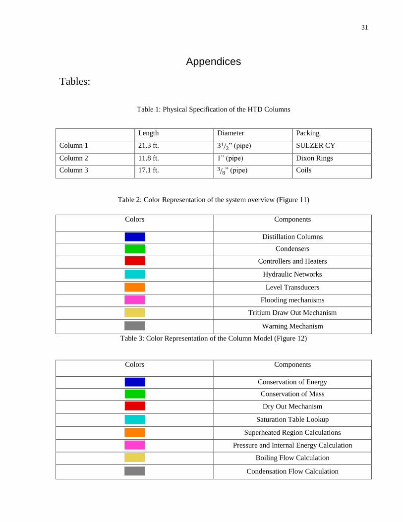
Table 1: Physical Specification of the HTD Columns

Length Diameter Packing

Column 1 21.3 ft. 3 ” (pipe) SULZER CY

Column 2 11.8 ft. 1” (pipe) Dixon Rings

Column 3 17.1 ft. ” (pipe) Coils

Table 2: Color Representation of the system overview (Figure 11)

Colors Components

Distillation Columns

Condensers

Controllers and Heaters

Hydraulic Networks

Level Transducers

Flooding mechanisms

Tritium Draw Out Mechanism

Warning Mechanism

Table 3: Color Representation of the Column Model (Figure 12)

Colors Components

Conservation of Energy

Conservation of Mass

Dry Out Mechanism

Saturation Table Lookup

Superheated Region Calculations

Pressure and Internal Energy Calculation

Boiling Flow Calculation

Condensation Flow Calculation

32

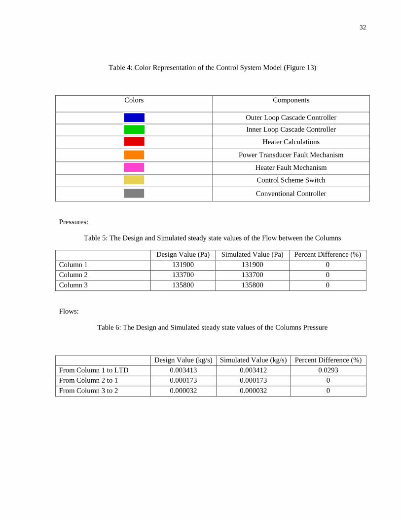
Table 4: Color Representation of the Control System Model (Figure 13)

Colors Components

Outer Loop Cascade Controller

Inner Loop Cascade Controller

Heater Calculations

Power Transducer Fault Mechanism

Heater Fault Mechanism

Control Scheme Switch

Conventional Controller

Pressures:

Table 5: The Design and Simulated steady state values of the Flow between the Columns

Design Value (Pa) Simulated Value (Pa) Percent Difference (%)

Column 1 131900 131900 0

Column 2 133700 133700 0

Column 3 135800 135800 0

Flows:

Table 6: The Design and Simulated steady state values of the Columns Pressure

Design Value (kg/s) Simulated Value (kg/s) Percent Difference (%)

From Column 1 to LTD 0.003413 0.003412 0.0293

From Column 2 to 1 0.000173 0.000173 0

From Column 3 to 2 0.000032 0.000032 0

33

Control Parameters:

Column 1:

Table 7: Column 1 Control Parameters

PID Controller Cascade Controller Optimized Controller

Outer Loop P 0.42 0.2 0.42

Outer Loop I 7e-4 3.3333e-004 7e-4

Outer Loop D 0 0 0

Inner Loop P N/A 0.2 1

Inner Loop I N/A 3.3333e-004 0

Inner Loop D N/A 0 0

Column 2:



Outer Loop P 0.5 0.5 0.5

Outer Loop I 0.0012 0.0012 0.0012

Outer Loop D 0 0 0




Column 3:



Outer Loop P 0.667 0.667 0.667

Outer Loop I 0.0056 0.0056 0.0056

Outer Loop D 40.02 40.02 40.02




34

Figures

Figure 1: Block Diagram of DTRF Process

Distillation

Columns

DTO/D2Power Plant

D2

DTD2O

DTO

T2

Figure 2: Tritium Removal Facility, Catalyst Exchange and Distillation

35

VPCE

FTS

DU

Expansion Tank

DMSRS

AU

LTD

HTD

CRS

D2O D2O/DTO

D2OHDO/D2O

T2

O2O2

D2/DT

D2

D2

Figure 3: Tritium Removal Facility, Flow Diagram

36

TH

D C

olu

mn

3

TH

D C

olu

mn

2

TH

D C

olu

mn

1

LT

D

Ca

taly

st C

on

ve

rte

r

He

at E

xch

an

ge

r 2

He

at E

xch

an

ge

r 1

Co

nd

en

se

r 3

Co

nd

en

se

r 2

Co

nd

en

se

r 1

Exp

an

sio

n T

an

k

Figure 4: High and Low Tritium Distillation Columns

37

Figure 5: Normal Packing Configuration

38

Figure 6: Packing Configuration during Flooding

39

Firing Board

Transducer

TRIAC

L1

N

4 – 20 mA

From DCI 4000

120 VAC

12

0 V

AC

Cla

ss

IV S

up

ply

To

He

ate

r

Fu

se

Fu

se

Fu

se

Figure 7: Heater Control, Wiring Diagram

40

Figure 8: Node/Link Figure

Figure 9: Nodal Representation of a Column

NjLkNi

41

Figure 10A: PID controller Block Diagram

Figure 10B: Cascade Controller Block diagram

Setpoint (r) PID-+

Plant

Control Loop

Error (e) Control Signal (u)

PID-+

PlantPower Transducer-+

Inner Loop

Outer Loop

PID(r1) (e1) (u1) (r2) (e2) (u2)

r1 = Outer Loop Setpoint

r2 = Inner Loop Setpoint

e1 = Outer Loop Error

e2 = Inner Loop Error

u1 = Outer Loop Control Signal

u2 = Inner Loop Control Signal

42

Figure 11: System Overview (See Table 2 for color representation)

43

Figure 12: Single Entry of Warning Mechanism

44

Figure 13: Column Overview (See Table 3 for color representation)

45

Figure 14: Control System Overview (See Table 4 for color representation)

46

Figure 15: Condenser 1 Level, Plant Data, Feb 14, 2011 Figure 16: Condenser 1 Level, Condenser 1, HTD Model

Figure 17: Column 1 Apparent Level6, Plant Data, Feb 14, 2011 Figure 18: Column 1 Apparent Level, HTD Model

6 Apparent level for all column levels is dimensionless. Apparent level is derived from temperature and is an estimation of the level trend not the absolute level

value.

20

25

30

35

40

18:25 18:36 18:48 19:00

Condenser 1 Level

Time (hh:mm)

Leve

l (%

)

20

25

30

35

40

0 100 200 300 400 500 600

Condenser 1 Level

Time (s)

Leve

l (%

)

50

70

90

110

18:25 18:36 18:48 19:00

Column 1 Level

Time (hh:mm)

50

70

90

110

0 100 200 300 400 500 600

Column 1 Level

Time (s)

47

Figure 19: Condenser 1 Level, Plant Data, Jan 01, 2011 Figure 20: Condenser 1 Level, Condenser 1, HTD Model

Figure 21: Column 1 Apparent Level, Plant Data, Jan 01, 2011 Figure 22: Column 1 Apparent Level, HTD Model

15

20

25

30

35

40

45

22:49 22:53 22:56 22:59

Condenser 1 Level

Time (hh:mm)

Leve

l (%

)

15

20

25

30

35

40

45

0 100 200 300 400 500 600

Condenser 1 Level

Time (s)

Leve

l(%

) 50

52

54

56

58

60

62

64

66

68

22:49 22:53 22:56 22:59

Column 1 Level

Time (hh:mm)

56

58

60

62

64

66

68

70

72

74

0 70 140 210 280 350 420 490 560

Column 1 Level

Time (s)

48

Figure 23: Column 2 Apparent Level, Plant Data, Jan 27, 2011

Figure 24: Column 2 Apparent Level, HTD Model

-200

-150

-100

-50

0

50

100

150

13:38 14:08 14:38 15:08 15:38

Column 2 Level

Time (hh:mm)

-200

-150

-100

-50

0

50

100

150

0 1800 3600 5400 7200

Column 2 Level

Time (s)

49

Figure 25: PID Controller, No Fault, Column 1

Figure 26: Proposed Cascade Controller, No Fault, Column 1

Figure 27: Optimized Cascade Controller, No Fault, Column 1

0 50 100 150 200 250 300 350 400 450 50050

60

70

80

90

100

110

Appare

nt

Level

Time(s)

0 50 100 150 200 250 300 350 400 450 50050

60

70

80

90

100

110

Appare

nt

Level

Time(s)

0 50 100 150 200 250 300 350 400 450 50050

60

70

80

90

100

110

Appare

nt

Level

Time(s)

50

Figure 28: PID Controller, Heater Fault, Column 1

Figure 29: Proposed Cascade Controller, Heater Fault, Column 1

Figure 30: Optimized Cascade Controller, Heater Fault, Column 1

0 50 100 150 200 250 300 350 400 450 50050

60

70

80

90

100

110

Appare

nt

Level

Time(s)

0 50 100 150 200 250 300 350 400 450 50050

60

70

80

90

100

110

Appare

nt

Level

Time(s)

0 50 100 150 200 250 300 350 400 450 50050

60

70

80

90

100

110

Appare

nt

Level

Time(s)

51

Figure 31: PID Controller, Power Transducer Fault, Column 1

Figure 32: Proposed Cascade Controller, Power Transducer Fault, Column 1

Figure 33: Optimized Cascade Controller, Power Transducer Fault, Column 1

0 50 100 150 200 250 300 350 400 450 50050

60

70

80

90

100

110

Appare

nt

Level

Time(s)

0 50 100 150 200 250 300 350 400 450 50050

60

70

80

90

100

110

Appare

nt

Level

Time(s)

0 50 100 150 200 250 300 350 400 450 50050

60

70

80

90

100

110

Appare

nt

Level

Time(s)

52

Fig 34: PID Controller, Column 1

Figure 35: Proposed Cascade Controller, Column 1

Figure 36: Optimized Cascade Controller, Column 1

0 50 100 150 200 250 300 350 400 450 50050

100

150

200

250

300

Appare

nt

Level

Time(s)

0 50 100 150 200 250 300 350 400 450 50050

100

150

200

250

300

Appare

nt

Level

Time(s)

0 50 100 150 200 250 300 350 400 450 50050

100

150

200

250

300

Appare

nt

Level

Time(s)

53

Fig 37: PID Controller, Column 2

Figure 38: Proposed Cascade Controller, Column 2

Figure 39: Optimized Cascade Controller, Column 2

0 1000 2000 3000 4000 5000 6000 7000-200

-150

-100

-50

0

50

100

150

Appare

nt

Level

Time(s)

0 1000 2000 3000 4000 5000 6000 7000-200

-150

-100

-50

0

50

100

150

Appare

nt

Level

Time(s)

0 1000 2000 3000 4000 5000 6000 7000-200

-150

-100

-50

0

50

100

150

Appare

nt

Level

Time(s)

54

Fig 40: PID Controller, Heater Fault for three columns, Column 2

Figure 41: Proposed Cascade Controller, Heater Faults, Column 2

Figure 42: Optimized Cascade Controller, Heater Fault, Column 2

0 50 100 150 200 250 300 350 400 450 500

20

40

60

80

Appare

nt

Level

Time(s)

0 50 100 150 200 250 300 350 400 450 500

20

40

60

80

Appare

nt

Level

Time(s)

0 50 100 150 200 250 300 350 400 450 500

20

40

60

80

Appare

nt

Level

Time(s)

55

Figure 43: PID Controller, Transducer Fault for three columns, Column 2

Figure 44: Proposed Cascade Controller, Power Transducer Fault, Column 2

Figure 45: Optimized Cascade Controller, Power Transducer Fault, Column 2

0 50 100 150 200 250 300 350 400 450 500

20

40

60

80

Appare

nt

Level

Time(s)

0 50 100 150 200 250 300 350 400 450 500

20

40

60

80

Appare

nt

Level

Time(s)

0 50 100 150 200 250 300 350 400 450 500

20

40

60

80

Appare

nt

Level

Time(s)

Documents

Tritium Removal Facility High Tritium Distillation Simulation · ii Tritium Removal Facility High Tritium Distillation Simulation Polad Zahedi Master’s of Applied Science Department