Embed Size (px)
Citation preview

N92-15458
Trends in StratosphericTemperature
Panel Members
M. R. Schoeberl, Chapter ChairP. A. Newman, Observations Subgroup Chair
J. E. Rosenfield, Modeling Subgroup Chair
J. AngellJ. BarnettB. Boville t,) }4 3 t _?aS. Chandra
S. Fels
E. FlemingM. GelmanK. Labitzke _ _2 If _-_l
A. J. Miller
J. Nash
V. RamaswamyF. Schmidlin
M. SchwarzkopfK. Shine
PRECEDING PAGE BLAi"JK NOT FILMED
i
I_|
_=
|!|l=
|
!

Chapter 6
Trends in Stratospheric Temperature
Contents
INTRODUCTION .......................................................... 447
TEMPERATURE DATA SET DESCRIPTION ................................... 447
6.2.1 Radiosonde ........................................................... 447
6.2.1.1 Introduction ................................................... 4476.2.1.2 Radiosonde Errors .............................................. 447
6.2.1.3 Description of the Radiosonde Data Sets .......................... 4486.2.2 Satellite .............................................................. 450
6.2.2.1 Introduction ................................................... 450
6.2.2.2 Radiance Data .................................................. 452
6.2.2.3 NMC Analyses ................................................. 4546.2.3 Rocketsonde .......................................................... 458
6.2.3.1 Introduction ................................................... 458
6.2.3.2 Corrections .................................................... 458
6.2.3.3 Rocket Data Base ............................................... 459
6.2.3.4 Accuracy and Precision ......................................... 4606.2.3.5 Trend Detection ................................................ 461
6.2.3.6 Summary ...................................................... 461
6.3 DATA ANAYLSIS .......................................................... 462
6.3.1 Intercomparisons ..................................................... 462
6.3.2 Short-Term Change and Long-Term Trends ............................. 472
6.4 MECHANISMS FOR ATMOSPHERIC TEMPERATURE TRENDS ............... 485
6.4.1 Global Ozone Changes .......... i ..................................... 485
6.4.2 The Radiative Impact of Other Trace Gases .............................. 489
6.4.3 Solar Cycle ........................................................... 4896.4.4 Aerosols ............................................................. 490
6.4.5 Dynamics ............................................................ 4946.4.6 Radiative Photochemical Models ........................................ 495
6.5 CONCLUSIONS ........................................................... 496
INT[ tONNZlPRSCEDING P_C,E B,_A,''_'_K NOT FILMED
445

m
z
I
m
=.
STRATOSPHERIC TEMPERATURE TRENDS
6.1 INTRODUCTION
The purpose of this chapter is to examine stratospheric temperatures for long-term and recent
trends, discuss the mechanisms that can produce atmospheric temperature trends, and deter-
mine if observed changes in upper stratospheric temperatures are consistent with observed
ozone changes.
The long-term temperature trends are determined up to 30 mb from radiosonde analysis
(since 1970) and rocketsondes (since 1969 and 1973) up to the lower mesosphere principally in the
Northern Hemisphere. The more recent trends (since 1979) incorporate satellite observations.
Previously published stratospheric temperature trend analyses used a variety of statistical
techniques and data bases; as a result, intercomparison has been difficult. Here, data sets from
the Free University of Berlin, the U.S. National Meteorological Center (NMC) of the National
Oceanic and Atmospheric Administration (NOAA), the United Kingdom Meteorological Office
(UKMO), and radiosonde and selected rocketsonde information are compared. The data set
descriptions, intercomparisons, and trends make up Sections 6.2 and 6.3 of this report.
In Section 6.4, the mechanisms that can produce recent temperature trends in the strato-
sphere are discussed. The following general effects have been considered: changes in ozone,
changes in other radiatively active trace gases, changes in aerosols, changes in solar flux, and
dynamical changes. Radiative equilibrium experiments have been performed with carefullycalibrated radiative transfer codes to quantify the magnitude of the temperature changes
expected with ozone and solar flux changes. In particular, computations have been made to
estimate the temperature changes associated with the upper stratospheric ozone changes
reported by the SBUV instrument aboard Nimbus-7 and the SAGE instruments. The conclusions
of this report are given in Section 6.5.
6.2 TEMPERATURE DATA SET DESCRIPTION
6.2.1 Radiosonde
6.2.1.1 Introduction
Radiosondes continue to provide the basic upper air data for meteorological services. The
users are a diverse group, including meteorologists who are involved in operational numerical
weather analysis and forecasting, and climatologists who are interested in the long-term
variations of quantities such as temperature. The accuracy of the temperature, pressure, and
humidity measurements obtained from radiosondes is particularly important to these users.
However, the accuracy required for day-to-day operations is not the same as that required for the
study of long-term trends; understandably, it is the accuracy required by the former that hasreceived the most attention.
6.2.1.2 Radiosonde Errors
Specification of the errors of the various radiosonde systems in regular worldwide use has
proven difficult. A relatively inexpensive "standard" instrument for calibration purposes has
never been developed; in the absence of a reference instrument, different methods have been
used in an attempt to judge the quality of radiosonde instruments, including the evaluation of
447
PRECEDING PAGE BLAi_K NOT FILMED
STRATOSPHERICTEMPERATURETRENDS
day-night differences in observational reports. A very useful method of comparing the measure-
ment capabilities of radiosondes is instrumental intercomparison, whereby multiple radio-sondes are carried aloft on a single balloon.
The most recent, and largest ever, series of radiosonde intercomparisons, organized by the
WMO Commission on Instrument and Method of Observation (CIMO), was carried out at
Bracknell, England, in 1984, and at Wallops Island, Virginia, USA, in 1985 (Nash and Schmidlin,
1987). The main findings, based on eight radiosonde types used in the intercomparisons, are:
• The reproducibility of temperature measurements was about 0.2K in most cases.
• The reproducibility of pressure measurements varied from 0.5 to about 2.0 mb.
• Different radiosonde instruments showed different time constants of response, which can
lead to appreciable difference in temperature estimates at given levels.
• Performance of the pressure sensor can be critical to temperature estimates at heights above
20 mb (assignment of the temperature to an incorrect pressure level).
As an example of these problems, Figure 6.1 displays a plot of consistent temperature
differences for a variety of radiosonde instruments (reprinted from Nash and Schmidlin, 1987).
Above the 50 mb level, instrument differences can be larger than 1K. The number of different
types of radiosonde in use at any time is not small (-17). Thus, the continuity and accuracy of
long-term trends are also subject to errors caused by modifications in design, manufacture, anddata reduction.
These findings have an obvious impact on operational analyses, in which accuracy isimportant, but their impact on trend analysis, in which precision is most important, may not be
as great. What is important in trend measurement is that the observations at individual stationsbe consistent in time; in the attempt to improve accuracy based on the above findings, it is this
consistency that is lost. It is not clear that the operational radiosonde network now in place will
ever prove entirely satisfactory for the detection of long-term variations in quantities such as
temperature. Nevertheless, radiosondes provide, and probably will continue to provide, the
primary data set for long-term lower stratospheric temperature trend assessment.
6.2.1.3 Description of the Radiosonde Data Sets
Two radiosonde-based data series are readily available for the investigation of long-term
temperature and geopotential height changes in the lower stratosphere, such as 30 mb. The
Northern Hemisphere daily analyses, carried out by the Stratospheric Research Group of the
Free University of Berlin, are based mainly on radiosonde observations at 00 and 12 UT (about
900 observations per day). Since 1980, these analyses have included satellite data taken over the
oceans (Labitzke et al., 1985). Because these analyses are a research project, carried out only after
all data have been received, consistency in time is achieved. The daily charts are digitized on a 10
by 10 latitude-longitude grid, and monthly zonal-mean temperatures are obtained. Over themiddle latitudes, each monthly zonal mean value of temperature is based on approximately
3,000 observations, resulting in a extremely small sampling error. Another advantage of this
technique is that errors of single stations on single days can be eliminated by comparison with
other stations nearby, and missing data can be interpolated. This data set starts in July 1964 for
most stratospheric pressure surfaces.
448
=
=
L
E
E

STRATOSPHERIC TEMPERATURE TRENDS
10
3o
50_0
13-
ILl
n'- 100O_00iii
ITrl
300
5OO
lOOO
DARKNESS 2300 GMT
\\x
BEUKERS-"_\
\\
INDIA
\
1 R
CORRECTION REMOVED
(a)
-2
GRAW M60
I
6,
I 6c I
-1 0 1
AT=[T i 0.5(TusA + TFIN)]'_C
I
2 0
//ZG,AW1.zg M60
//INDIA
",_" OTHERS
0.5
AT_C
(3-
W
IT"
09W
CCrl
_o
3O
5O
1oo
DARKNESS 2300 GMT
_ _FFIG
"" ...GRAW M60
BEUKEFIS ,--_ .
\\
\
i I
300 /z
7
500
AUSTRALIA
_AND
(b)
lOOO I__ • J-3 -2 -1 o 1 2 3
3T=_T, - l:).51'Tus,_+ T_,v)J°C
Figure 6.1 Intercomparison of different radiosondes at night (from Nash and Schmidlin, 1987). T_ is the
temperature measured by the particular instrument. (a) Temperature differences from a standard defined by
the U.S. and Finnish instruments. (b) As in (a), but reported on standard pressure surfaces. Note the
increased error caused by the information in the pressure sensor.
449

STRATOSPHERIC TEMPERATURE TRENDS
The second temperature series, from Angell and Korshover (1983a), is based on the variation
of height difference or thickness (proportional to mean temperature) between 100 and 30 mb at
63 radiosonde stations distributed worldwide, 45 of which are in the Northern Hemisphere. At
each station for each year, the seasonal deviation of thickness from the long-term seasonal meanhas been determined; these station deviations have then been averaged for polar, temperate,
subtropical, and equatorial zones, as well as for both hemispheres and the world, by the use of
area weighting. This data set generally begins in 1958, but because Soviet Union radiosonde data
were not available before 1970, the temperature variations in north polar and north temperate
climatic zones are not represented before that date. Because of the relatively small number of
radiosonde stations used in this analysis, this technique is much more sensitive to erroneous
station data or missing data than is the previous technique. The two data sets are intercomparedin Section 6.3.1.
6.2.2 Satellite
6.2.2.1 Introduction
Before 1978, several satellite temperature sounders were in use with weighting functions in
the stratosphere and mesosphere, including the Vertical Temperature Profile Radiometer
(VTPR), the Selective Chopper Radiometer (SCR), and the Pressure Modulated Radiometer
(PMR). Data from these have not been used for trend analysis because the available data are not
of sufficient accuracy or record length. For example, the PMR data for the upper stratosphere and
mesosphere would have been of particular interest but, although the instrument appeared to bestable, the data record extended only for 3 years.
The TIROS-N Operational Vertical Sounder (TOVS) Series began operation in late 1978.
TOVS comprises three radiometers that provide observations of narrow bandwidth radiance,
originating primarily from the stratosphere and troposphere. The radiometers are the High-resolution Infrared Sounder (HIRS-2), the Stratospheric Sounding Unit (SSU), and the Micro-
wave Sounding Unit (MSU); their nominal performance is outlined in Smith et al. (1979). Theseinstruments measure the thermal emission from layers of the atmosphere, as indicated by the
weighting functions given in Figure 6.2a. The present series of the TIROS-N spacecraft is
expected to remain in operation beyond 1990; hence, the current type of sounders has the
potential to provide a monitor of stratosphere temperature trends over at least 10 years.However, because not all of the spacecraft will carry the principal stratosphere sounder, the SSU,
the quality of trend information can be expected to diminish during the rest of the decade.
These emitted radiances from Earth's atmosphere may be individually converted to an
equivalent temperature for each layer (known as the brightness temperature) or may be retrieved
to obtain a temperature profile or layer mean temperature between fixed pressure levels. Itshould be noted that the measurements are obtained on a vertical pressure scale (as opposed to
height).
Two methods for determining stratospheric temperature changes from the TOVS data will be
discussed. Nash and Forrester (1986) used the zonal mean measurements from several radiom-
eter channels. Their work was aimed primarily at trend-type studies, without performing any
temperature retrieval. They established reproducibility and systematic drifts in both the radio-
metric (i.e., temperature) and the spectroscopic (i.e., weighting function) performance by
careful comparison between different sounders in simultaneous operation and by careful
prelaunch calibration. Estimates of temperature trends since late 1979 were derived for layers of
45O
=
ZE
R_
Z

STRATOSPHERIC TEMPERATURE TRENDS
J_
X SSU15 m /N,_02 CHANNELS/Y_
10
f I MSU SSUCH. 25 -\ -,>(
I X / -0..24
100
1000
0.01
I
003
0.1
0.3
E 1
3
v
lO
3o
lOO
3oo
0 0.2 0.4 0.6 0.8 1.0 -0.2
NORMALIZED WEIGHTING FUNCTION
SYNTHESIZED
CHANNELS
SSU"" CH. 36X
: SSU CH. 26X
I .-'" "_I
/--SSU CH. 15X.* ,
.' /
.." /•
.°" /*
.:./" (b)
I I I L. I ,0 0.2 0.4 0.6 0.8
NORMALIZED WEIGHTING FUNCTION
0.9
Figure 6.2 Weighting functions for satellite temperature instruments: (a) MSU, SSU; (b) Synthesized SSUchannels from Nash (1987).
451

STRATOSPHERIC TEMPERATURE TRENDS
the atmosphere centered at pressures between 90 and 0.5 mb. Their method is discussed in detailin Section 6.2.2.2.
Gelman et al. (1986) use global stratospheric temperature fields derived as an operationalproduct from the National Meteorological Center. In contrast to the Nash and Forrester method,
a temperature retrieval process is used first to give temperatures as a function of latitude,
longitude, and pressure. Because data from only one satellite are used at any one time, periods of
overlap are not available for intercomparison. The fields were retrospectively adjusted (primarilyusing comparisons with rocketsonde data) to compensate for differences between the successivesatellites in the TIROS-N series. This data set is discussed in Section 6.2.2.3.
6.2.2.2 Radiance Data
NOAA spacecraft have been in simultaneous operation for most of the time since late 1978.
Comparison of observations obtained by the nominally identical TIROS Operational VerticalSounders (TOVS) from two simultaneously operated spacecraft in the TIROS-N/NOAA series
has allowed a check on the stability of their radiometer performance.
The comparison data used in this report were previously described by Nash and Forrester(1986) and were obtained by an extension of the methods used in earlier studies of 5SU
performance by Pick and Brownscombe (1981) and Nash and Brownscombe (1983).
The TOVS channels chosen for analysis have been limited to those with relatively highvertical resolution (i.e., 10 to 15 km), namely MSU and SSU. The stratospheric HIRS-2 channels
have poor vertical resolution and contribute only redundant information. Processed radiance
observations from these channels have been separated according to radiometer view angle andused to generate zonally averaged mean radiances for 10 latitude bands centered from 70°N to
70°S for each day. Radiances from the nadir or near-nadir views have been used in each case.
Further independent information is obtained through a procedure described by Nash (1988) inwhich differences are taken between the zonal mean SSU radiances at 35 ° and 5° to nadir. The 35 °
weighting functions are at higher altitudes (because of limb effects), and combinations can be
found that are either sharper than the contributing weighting functions or at higher altitudes.
This technique provides the highest altitude weighting function, known as 47X, which is
centered at about 0.5 mb (approximately 54 km). Figure 6.2b gives the weighting functions forthese synthesized channels.
The consistency between the TOVS channels has been examined by computing the difference
between the zonally averaged radiances obtained for the north- and southbound portions of theorbit at each latitude. Because the NOAA spacecraft are in Sun-synchronous orbits, the nadir-
view observations at a given latitude are always for fixed local times, which are about 12 hours
apart at most latitudes for a given spacecraft. Observation local times were about 0300 and 1500hours for TIROS-N, NOAA-7, and NOAA-9, and about 0700 and 1900 hours for NOAA-6 and
NOAA-8. The existence of diurnal and semidiurnal solar tides is a major complication becausethey lead to consistent biases between the measurements at these various local times. A solardiurnal tide will cause a difference between the north- and southbound zonal means, but will not
affect their average except when their local times differ substantially from 12 hours. However, a
solar semidiurnal tide has the reverse effect of causing a bias in the north/southbound average,but producing zero difference in the zonal means. The lunar semidiurnal tide has an effect
similar to that of the solar semidiurnal tide, except that it has a 4-week periodicity; its effect was
eliminated here by averaging over monthly periods. For the diurnal cycle, which has the largest
E
F
m
452
STRATOSPHERIC TEMPERATURE TRENDS
amplitude at extratropical latitudes, solar tidal theory predicts maximum 12-hour differences of
less than 0.3K at 100 mb, less than 0.5K at 20 rob, and rising to a peak of about 6K at 2 mb. The
temperature is predicted to peak at about 1800 hours. The TOVS observations are compatible
with this theory. Not only are the 12-hour differences as expected (larger for the 0700-1900 hour
spacecraft), but so are the absolute differences between spacecraft.
For trend determination, it is important to distinguish between radiometric calibration and
spectroscopic errors, which are largely independent. A single channel will measure radiance (orbrightness temperature) corresponding to a weighting function. Radiometric calibration errors
cause the measured radiance to be incorrect, directly causing a temperature error. Spectroscopic
errors (such as errors in the filter wavelength or in the basic spectroscopic line data) will cause
errors, such as a vertical shift, in the weighting function; this leads indirectly to temperature
errors that will depend upon the lapse rate and, hence, upon the latitude and season. Both types
of error have various components of systematic bias, but some of these will be common to all
instruments of a given type or design. Thus, errors in spectral line data would be unimportant
when intercomparing SSU's, but would matter when comparing an SSU with an MSU, since the
two instruments view at quite different wavelengths. Nash and Forrester (1986) used measure-
ments of natural atmospheric variations that are height dependent (e.g., the tidal 12-hourdifference, seasonal variations) to intercompare the pressure levels viewed by different radiom-
eters and by radiosondes, and so establish which channels were observing at the correct level.Residual differences were then described as biases. The latitudinal variation of bias between the
different measurements for the same pressure level was also used as an indication of data quality
and of the types of instrument problems that could be occurring. Of crucial importance was the
apparent long-term stability of the NOAA-6 SSU and MSU. Although there were periods when
this satellite was not operated (because of the failure of the HIRS-2), there was enough overlap of
operation with other NOAA satellites to be confident of the long-term trends shown. Tempera-
ture values within these gaps were obtained from TOVS instruments on the other satellites, after
adjustments were made for identifiable radiometric and spectroscopic differences.
The overall conclusions regarding the accuracy of TOVS data for long-term trend studies are:
• Single TOVS channels can, in some cases, measure monthly zonal mean brightness
temperature to an accuracy of about 0.2K root mean square (rms) (1K for synthesized
channels).
• The data sets obtained from several satellites indicate that the NOAA-6 SSU and MSU were
stable over the period 1980--1986 to the same order of accuracy.
Because the atmospheric mixing ratio of carbon dioxide is increasing at a rate of about 0.4
percent per year, the weighting function for a spectroscopically stable SSU channel moves
upwards, causing a change in the measured brightness temperature that depends on the lapse
rate. Line-by-line calculations have been made of the effects of an 8 ppmv increase in the carbon
dioxide mixing ratio, corresponding to the change from 1979-1980 to 1985-1986, for an annual
mean 30°N temperature profiles. These changes (listed in Table 6.1) are substantially smaller
than the trends observed, so it is concluded that these effects play only a minor role. Oxygenmixing ratios are proportionally much more stable than those of carbon dioxide, and any trend
for the MSU weighting functions should be negligible. Another potential source of error is the
effect of ozone upon absorption in the 15-micron carbon dioxide band used by the SSU and HIRS
for temperature sounding. The use of gas correlation minimizes the effect of ozone on the SSU
measurements to the extent that it is not considered necessary to make any correction. However,
453

STRATOSPHERIC TEMPERATURE TRENDS
Table 6.1 Sensitivity of Measured SSU Brightness Temperatures to 8 ppmv COa Increase and 10Percent Ozone Decrease at all Levels
ChannelApparent Temperature Increase
Due to 8 ppmv CO2 Increase (K)
Apparent Temperature IncreaseDue to 10% Ozone Decrease (K)
47X - 0. 289 - 0.01
36X - 0. 072 - 0.04
27 0.00 0.0026 0.12 -0.01
25 0.14 -0.02
26X 0.182 0.02
15X 0.085 0.05
Table 6.1 gives the calculated apparent temperature changes caused by a 10 percent decrease of
ozone concentration. Any small ozone trend that might have occurred should have negligible
effect on the temperature trend measurements over this period. The corrections indicated inTable 6.1 have not been incorporated into the data set's satellite.
6.2.2.3 NMC Analyses
The NOAA series of polar-orbiting satellites has provided temperature soundings in supportof operational meteorological analyses for weather forecasting. As part of the regular operations
of the NMC, global fields have been produced of geopotential height and temperature at
stratospheric constant pressure levels 70, 50, 30, 10, 5, 2, 1, and 0.4 mb (corresponding toaltitudes from 18 to 55 km). The analysis system for the fields is a modified Cressman for both 70
to 10 mb levels (Finger et al., 1985) and 5 to 0.4 mb levels (Gelman and Nagatani, 1977). The
source of satellite data for the analysis, as well as the methodology for using these data in theanalysis system, have changed as improvements have been developed (Gelman et al., 1983).
Some changes were necessary because of instrumental failure or failure of specific instrument
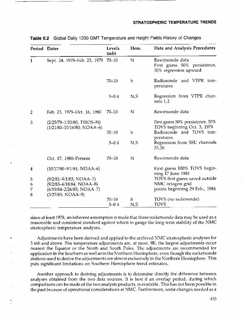
channels. Table 6.2 summarizes the principal changes that are relevant to a study of the
stratospheric fields (70 to 0.4 mb) for the Northern and Southern Hemisphere analyses. The
changes to the 70 to 10 mb system primarily have involved changes in the use of radiosonde data
for the Southern Hemisphere and in first-guess derivation. Changes for the upper stratosphere(5 to 0.4 mb) analyses relate to changes in satellites as well as in the use of TOVS data. Before
October 17, 1980, simple regression relationships from two channels of the VTPR or the SCR
were used. Temperature retrievals produced from TOVS provide layer mean temperature
between the standard pressure levels. Temperatures at the NMC analysis levels are found bylinear interpolation in log pressure of the layer mean temperatures.
As indicated in Table 6.1, there have been seven changes (eight periods) since the initiation of
the NMC global stratospheric analyses. Some basis must be provided for assuring stability of the
NMC analyses for determining interannual changes in stratospheric structure and long-term
trends in temperature. Therefore, meteorological rocketsonde and radiosonde temperatureshave been compared with temperatures interpolated to the locations of the rocket stations from
the analyzed field closest in time.
The error estimates for rocketsonde temperature data are I-3K over the altitudes 35 to 55 km
(see Section 6.2.3). Since both rocketsonde hardware and data observation procedures have beenstandardized for the stations in the Cooperative Meteorological Rocketsonde Network (CMRN)
454
STRATOSPHERIC TEMPERATURE TRENDS
Table 6.2 Global Daily 1200 GMT Temperature and Height Fields History of Changes
Period Dates Levels Hem. Data and Analysis Procedures(rob)
1 Sept. 24, 1978-Feb. 23, 1979 70-10 N Rawinsonde dataFirst guess 50% persistence,
50% regression upward
2
3
4
5
67
8
70-10 S Radiosonde and VTPR tem-
peratures
5-0.4 N,S Regression from VTPR chan-nels 1,2
Feb. 25, 1979-Oct. 16, 1980 70-10 N
(2/25/79-1/20/80; TIROS-N)
(1/21/80-10/16/80; NOAA-6)
Oct. 17, 1980-Present
(10/17/80-9/1/81; NOAA-6)
(9/2/81-9/1/83; NOAA-7)
(9/2/83-6/18/84; NOAA-8)
(6/19/84-2/26/85; NOAA-7)
(3/27/85; NOAA-9)
70-10 S
5-0.4 N,S
70-10 N
Rawinsonde data
First guess 50% persistence, 50%
TOVS beginning Oct. 3, 1979Radiosonde and TOVS tem-
peratures
Regression from SSU channels25,26
Rawinsonde data
First guess 100% TOVS begin-
ning 17 June 1981
TOVS first guess saved outside
NMC octagon grid
points beginning 29 Feb., 1984
70-10 S TOVS (no radiosonde)
5-0.4 N,S TOVS
since at least 1978, an inherent assumption is made that these rocketsonde data may be used as a
reasonable and consistent standard against which to gauge the long-term stability of the NMC
stratospheric temperature analyses.
Adjustments have been derived and applied to the archived NMC stratospheric analyses for
5 mb and above. The temperature adjustments are, at most, 9K; the largest adjustments occur
nearest the Equator or the North and South Poles. The adjustments are recommended for
application in the Southern as well as in the Northern Hemisphere, even though the rocketsondestations used to derive the adjustments are almost exclusively in the Northern Hemisphere. This
puts significant limitations on Southern Hemisphere trend estimates.
Another approach to deriving adjustments is to determine directly the difference between
analyses obtained from the two data sources. It is best if an overlap period, during which
comparisons can be made of the two analysis products, is available. This has not been possible in
the past because of operational considerations at NMC. Furthermore, some changes needed as a
_ 455

STRATOSPHERIC TEMPERATURE TRENDS
result of the failure of an instrument or specific channels precluded such an overlap period.
Therefore, Gelman et al. (1983) compared zonal average temperatures derived from the analyses
immediately before and after each change and tried to determine the nonmeteorological change
at each change date. This determination is most difficult at polar latitudes in winter and may not
be possible when there is a lapse in analyses of more than a few days, as was the case at the
beginning of period 8. Figure 6.3 shows these determinations (denoted by joint) for the Equator,
30°N, 30°S, 60°S, and 60°N for the 2-mb level over the eight adjustment periods (see Table 6.2).
Figure 6.3 (denoted by Rocket) also shows the changes implied by the rocket comparisons.
Another method of estimating these changes is by statistical evaluation. Estimates based on
this approach for 2 mb are also shown in Figure 6.3 (denoted by Step Regression) and are
discussed in detail by Gelman et al. (1983). The pattern of relative agreement among the different
methods depicted in Figure 6.3 is reasonably good. However, differences of 2-4K are common,
and uncertainty in adjustments of this magnitude should be expected.
LUr7<¢T
I--ZwO
03LUUJn-(.9LUD
0
-5
5
60N
t t t /% t = i 1 t /% t
[] O n
1oz_ r7 o o
o o A
I I I I I i . I I
30N
o
-5
5
o
-5
5
' ' ' ' ' 'to 9_ [] OZl
I I I I i _ i t I
EQUATOR
....... I I I I I I /
o [] o 1I I i _ I I I
30S
I I I I I I I I I IIo o 8 8 g
o-5 l _ I I I I 0 I I t
60S5
5
L I I I I I I I I I
[] o 8 8 go [] El
oL _ I, i : t 0 1 z t
1 2 3 4 5 6 7
PERIOD
Figure 6.3 Temperature changes in the 2 mb NMC analyses, as inferred from rocket comparisons (o,Rocket), comparison of analyses around change dates ([], Joint), and regression (a, Step Regression), as
explained in text.
456
STRATOSPHERIC TEMPERATURE TRENDS
EQUATOR
IVl'÷l.....6 F'I' ' '1] '1' 'll .... J' '1' ' J ' ' ' Iq _,lr , ill i l, , i i i , 8
4 -_
O 2
0
121 -
-4 F (a) ] _(c)
0 20 40 60 80 100 0 20 40 60 80 100 0 20 40 60 80 100
MONTHS MONTHS MONTHS
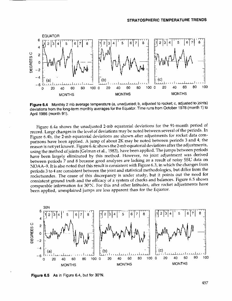
Figure 6.4 Monthly 2 mb average temperature (a, unadjusted; b, adjusted to rocket; c, adjusted to joints)deviations from the long-term monthly averages for the Equator. Time runs from October 1978 (month 1) to
April 1986 (month 91).
Figure 6.4a shows the unadjusted 2-mb equatorial deviations for the 91-month period of
record. Large changes in the level of deviations may be noted between several of the periods. In
Figure 6.4b, the 2-mb equatorial deviations are shown after adjustments for rocket data com-
parisons have been applied. A jump of about 2K may be noted between periods 3 and 4; the
reason is not yet known. Figure 6.4c shows the 2-mb equatorial deviations after the adjustments,
using the method of joints (Gelman et al., 1983), have been applied. The jumps between periods
have been largely eliminated by this method. However, no joint adjustment was derived
between periods 7 and 8 because good analyses are lacking as a result of noisy SSU data on
NOAA-9. It is also noted that this result is consistent with Figure 6.3, in which the changes from
periods 3 to 4 are consistent between the joint and statistical methodologies, but differ from the
rocketsondes. The cause of this discrepancy is under study, but it points out the need for
consistent ground truth and the efficacy of a system of checks and balances. Figure 6.5 shows
comparable information for 30°N. For this and other latitudes, after rocket adjustments have
been applied, unexplained jumps are less apparent than for the Equator.
O
09wwtT(.9w
6
4
2
0
-2
-4
-6
30N
' I4 ....5
J'6' '7 I"8''-_- ....i&"÷l....._
_L_j -(b), _L_L._ _L_L -.... l, ,, ,d_ l__ ! .... I ....
0 20 40 60 80 100 0 20 40 60 80
MONTHS MONTHS
41'1"1"1'""i r712345 .....8
100 0 20 40 60 80
MONTHS
i
00
Figure 6.5 As in Figure 6.4, but for 30°N.
457

STRATOSPHERIC TEMPERATURE TRENDS
The underlying theme of this discussion has been to determine to what degree a trend in "stratospheric temperature can be detected. On average, NMC analyses have had one major
change a year with a confidence factor of 2-3K. Thus, if NMC stratospheric analyses with current
adjustment techniques are used, a trend of less than 1.5K per decade over a decade would not be
detected; however, a decadal change of 4-5K would be detectable.
6.2.3 Rocketsonde
6.2.3.1 Introduction
The number of rocketsonde launch sites operated by the United States increased from aninitial 3 or 4 sites in 1958 to about 30 in 1965, and has since decreased to the present 9 sites. The
number of rocketsondes launched in the U.S. has also decreased, from 3 to 5 per week to about 3
to 5 per month--a serious limitation for detecting long-term trends.
Despite the long period of rocketsonde measurements that exists for the U.S., many of thelaunch sites are unsuitable for trend analysis because of short, and often incomplete, data
records. Nonetheless, the U.S. rocketsonde program has provided sufficient information from
14 launch sites (Table 6.3) to attempt an analysis of temperature trends. For this report, six sites
with the most complete long-term records will be discussed.
6.2.3.2 Corrections
When properly applied, rocketsonde temperature corrections should improve the estimate of
ambient temperature. Examples of optimal corrections applied to the Arcasonde and Datasondeinstruments are presented in Table 6.4 and applied to the same temperature profile, inde-
pendent of the instrument. The aerodynamic and radiation corrections are the dominantcontribution to the ._otal correction.
Table 6.3 Rocketsonde Launch Sites Having Data Available for Trend Analysis
Rocketsonde Site Latitude Longitude Observational Period
9°S 14°W 1969-19859°N 168°E 1979-1985
9°N 80°W 1969-1979
17°N 62°W 1969-1977
22°N 160°W 1969-198228°N 81°W 1969-1986
32°N 106°W 1969-1982
Ascension Island
Kwajalein, MIFt. Sherman, CZ
Antigua, BWI
Barking Sands, HICape Canaveral, FLWhite Sands Missile
Range, NM
Pt. Mugu, CA
Wallops Island, VA
Shemya, AKPrimrose Lake, Canada
Ft. Churchill, Canada
Poker Flat, AK
Thule, Greenland
34°N 119°W 1969-198238°N 75°W 1969-1980
53°N 174°E 1975-1985
55°N 110°W 1969-1982
59°N 94°W 1971-1979
65°N 148°W 1969-1978
77°N 69°W 1976-1981
NOTE: Data exist into 1986 for most of these sites. However, the reduction in the number of the U.S. rocketsondelaunchings beginning in the late 1970's inhibits analysis outside of above dates.
458

STRATOSPHERIC TEMPERATURE TRENDS
Table 6.4 Example of Arcasonde and Datasonde Measurements of Same Temperature Profiles
and Appropriate Corrections
Temp. Aero. Lag. Emissivity Radiation Correction Ambient
(K) Heating Temp.
Alt. = 40 km
Arcasonde 250.0 - 0.4 - 1.0 0.4 - 0.4 - 1.4 248.6
Datasonde 250.3 - 0.4 - 0.5 0.3 - 1.1 - 1.7 248.6
Alt = 45 km
Arcasonde 242.0 - 0.9 - 1.2 0.5 - 0.4 - 2.0 240.0
Datasonde 242.6 - 0.9 - 0.7 0.4 - 1.4 - 2.6 240.0
Alt -- 50 km
Arcasonde 261.0 - 2.1 - 1.7 0.9 - 0.5 - 3.4 257.6
Datasonde 261.9 - 2.2 - 0.9 0.7 - 1.9 - 4.3 257.6
NOTE: Corrections are from Krumins and Lyons (1972).
The interpretation of the temperature trend between 1971 and 1973 given by Johnson and
Gelman (1985) proposes that part of the sudden decrease in the temperature observed (-3K)could be attributed to a changeover in instrument design (i.e., from Arcasonde to Datasonde);
however, the decrease is still present when only Datasonde profiles are used (Schmidlin, private
communication). The Datasonde gradually replaced the Arcasonde at all U.S. ranges--at many
before 1971. Krumins and Lyons (1972) published Datasonde corrections in 1972 that generally
came into use at launch ranges in 1973. The initiation of corrections in 1973 might explain part of
the decrease reported by Johnson and Gelman. The magnitude of the correction, if applied,would be about - 1.0K at 40 km and about - 1.6K at 45 km--approximately the amount of the
difference noted between 1971 and 1973.
6.2.3.3 Rocket Data Base
All of the U.S. rocketsonde data available in the archive from 1969-1986 were examined. Data
obtained before 1969 were not used because of the different data format. In addition, diverse
instrument designs were used at some ranges until about 1971 and, in a few cases, even as late as
1973. Because the measurement quality of these systems varied from one instrument design tothe other, the data from these instruments were not used. The rocket data base includes only
Arcasonde and Datasonde data.
To eliminate the possibility of any discontinuity in the use of the corrections of Krumins and
Lyons (1972) at any of the sites listed in Table 6.3, the data were examined for 1972 through 1986to determine whether the standard U.S. correction was applied. If corrections had not been
applied, they were incorporated. Furthermore, the temperature data obtained between 1969 and1972 were also corrected using the same procedure. Thus, the temperature trend analyses
presented here are produced from a consistent and homogeneous group of corrected tempera-ture measurements extending from 1969 to the present.
It should be noted that even though the data set may now be considered uniform throughout,bad measurements were found in the profiles (as a result of bad calibrations or depressed
_ 459
STRATOSPHERIC TEMPERATURE TRENDS
sensors, for example) and had to be eliminated. The data from the 14 sites selected for analysis
were plotted with the accompanying conjunctive rawinsonde. Profiles that showed differencesof 3K or more throughout their overlapping altitudes were subsequently deleted. No attemptwas made to determine whether the fault was in the radiosonde or the rocketsonde data. The
consequence of this editing was a reduction in the number of observations available for analysis
by about 35 percent. Despite the removal of a large number of observations, sufficient data were
available with a reasonable temporal distribution to produce the monthly averages used in the
trend analysis.
The steps followed to obtain a valid and consistent data set for trend analysis can besummarized as follows:
• Only Arcasonde and Datasonde profiles from 1969 through 1986 were selected for analysis.
All rocketsonde profiles from 1969 to 1972 were edited and quality checked by comparing
them with the supporting radiosonde; if temperature differences of 3K or more were
present, the rocketsonde observation was deleted.
• All uncorrected profiles were corrected, using the standard method.
6.2.3.4 Accuracy and Precision
Direct analysis of accuracy is difficult for rocketsonde instruments because of the lack of a
reference standard. Although occasional Datasonde instruments give data profiles that disagree
with the conjunctive radiosonde profile, a number of instruments were recalibrated after 2 years
and found unchanged (Schmidlin, 1981). Thus, any disagreement between the rocketsonde and
radiosonde temperatures is usually the result of bad calibration, an improperly mountedthermistor, or a bad radiosonde measurement. Poor data from these sources were removed as far
as possible. However, true inflight accuracy is difficult to specify; hence, the need for correc-
tions. Corrections should be known well enough to enable ambient temperatures to be produced
from the thermistor temperature.
The accuracy of the Datasonde temperature sensor has been estimated as 3-5K, based on
comparisons between 1) various rocket techniques (Olsen et al., 1979; Schmidlin, 1984), 2)
rocketsonde instrument designs (Finger et al., i975; Olsen et al., 1979), and 3) satellite instru-
ments (Barnett et al., 1974; Barnett and Corney, 1984; and Pick and Brownscombe, 1981). Arecent comparison of overlapping Datasonde thermistor and falling sphere measurements
between 30 and 60 km (Schmidlin, private communication) revealed excellent temperatuie
agreement to within the limits of the variability in the measurements. The inflatable sphere's
measurement is independent of the external influences that disturb thermistor measurements
(e.g., aerodynamic heating and radiation errors), so that this agreement suggests that Datasondeaccuracy is probably near IK up to an altitude of 60 km.
An analysis of paired measurements (Schmidlin, 1981) using 21 pairs of Datasonde, with theinstruments of each pair launched 5 minutes apart, gave an estimate of repeatability of 0.8K at 35
km and 1.3K at 50 km. Through the use of an indirect method for estimating errors found in
Gandin (1963), the precision of the Datasonde was calculated to be 0.6K at 35 km and 0.9K at 50km.
460 "-
STRATOSPHERIC TEMPERATURE TRENDS
6.2.3.5 Trend Detection
Initial trend analysis carried out for the 40 and 45 km altitudes using unedited Wallops Island
and Cape Canaveral observations, respectively, indicated a temperature decrease of approxi-
mately - 0.35K per year. This rather large downward trend was determined for 1969-1986 usingall of the data existing in the archive (including the unqualified rocketsondes, uncorrected
profiles, and corrected profiles). Regression of the edited Cape Canaveral and Wallops Islandmonthly averages for the same altitudes showed trends of approximately - 0.22 ° per year and
- 0.18 ° per year, respectively. Thus, the difference between the edited data used here and the
unedited data can be very large.
Because of the sudden temperature decrease (between 1971 and 1973) reported by Johnson
and Gelman (1985), it was considered important to attempt to determine whether the tempera-
ture drop originated from the Arcasonde to Datasonde changeover. Schmidlin (private commu-
nication) has separated Datasonde observations from all others in the 1970-1973 timeframe.From these Datasonde observations it is clear that a 2K drop in temperature still exists at most
rocket stations. At the time of writing, it is still not clear whether this drop in temperature is due
to undetected instrumental problems or to a real atmospheric change. Further work on this point
is clearly warranted. Trends should be calculated separately for 1969-1986 and 1973-1986.
Since the sample size was reduced by about 35 percent after eliminating all suspect observa-tions, as described above, there is some concern that the gaps between monthly averages were
more frequent than desired and might lead to erroneous results. Consideration was given to
using the longest complete data periods to reduce the error caused by the smaller segments ofdata. Only a handful of the 14 stations had sufficiently long data records to permit trend
analyses. Trends were calculated between 1973 and the latest date possible for 4 of the 14 sites.
The averages calculated for each altitude (30, 35 ..... 55 km) are actually derived from 5-kmvertical intervals (i.e., 30 km is an average of the temperatures between 28 and 32 km). Monthly
averages are composed of the observations within a given month, with a minimum of threeobservations. When multiple observations occurred within the same day, only one observation
for that day was included. Furthermore, it was important to reduce the effect that tidal activity
might have had on the trend calculations. Therefore, only observations made in daylight were
used. An attempt to use a more restricted time period of 2 or 4 hours centered about midday
failed because then the sample size became too small.
6.2.3.6 Summary
A careful examination of the rocketsonde data for the 1969-1986 period, and elimination of
the profiles that disagreed with the supporting radiosondes, reduced the data set by about 35
percent. If the standard U.S. correction had not been applied, the rocketsonde data were
corrected following Krumins and Lyons (1972).
Monthly averages over the period 1969 to the end of the data set were calculated using
daylight observations only; nighttime observations were avoided to reduce any biasing effect
that might be created from the diurnal tide. Monthly averages comprise at least three observa-tions. Johnson and Gelman (1983), using the unedited rocketsonde data, showed an average
temperature decrease of 3.4K in the 25 to 30 kin, 25 ° to 55°N region between 1970 and 1972, while
the support radiosondes showed only a 2K change. However, the edited rocketsonde data setused here shows temperature decreases of 3.3K, 2.2K, 1.6K, 1.2K, and 2.9K at Cape Canaveral,
461
STRATOSPHERIC TEMPERATURE TRENDS
White Sands, Pt. Mugu, Wallops Island, and Primrose Lake over a 28 to 32 km altitude range forthe same period. The average of these stations is in better agreement with the support radio-
sonde change, suggesting that the editing of biased rocketsondes and the application ofcorrections to uncorrected data may have alleviated much of the difference.
6.3 DATA ANALYSIS
6.3.1 Intercomparisons
In previous studies of stratospheric temperature trends, little attempt was made to inter-
compare data sets. The object of this section is to make the comparisons among the various data
sets available for trend assessments and to provide a data quality check for long-term trendcomputations.
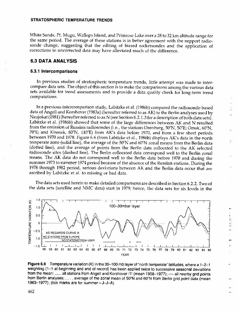
In a previous intercomparison study, Labitzke et al. (1986b) compared the radiosonde-based
data of Angell and Korshover (1983a) (hereafter referred to as AK) to the Berlin analyses used by
Naujokat (1981) (hereafter referred to as N (see Section 6.2.1.3 for a description of both data sets).Labitzke et al. (1986b) showed that some of the large differences between AK and N resulted
from the omission of Russian radiosondes (i.e., the stations Orenburg, 50°N, 50°E; Omsk, 60°N,
70°E; and Kirensk, 60°N, 110°E) from AK's data before 1970, and from a few short periodsbetween 1970 and 1978. Figure 6.6 (from Labitzke et al., 1986b) displays AK's data in the northtemperate zone (solid line), the average of the 50°N and 60°N zonal means from the Berlin data
(dotted line), and the average of points from the Berlin data collocated to the AK selected
radiosonde sites (dashed line). The Berlin collocated data correspond well to the Berlin zonal
means. The AK data do not correspond well to the Berlin data before 1970 and during the
summer 1973 to summer 1974 period because of the absence of the Russian stations. During the1978 through 1982 period, serious deviations between AK and the Berlin data occur that are
ascribed by Labitzke et al. to missing or bad data.
The data sets used herein to make detailed comparisons are described in Section 6.2.2. Two ofthe data sets (satellite and NMC data) start in 1979; hence, the data sets for six levels in the
1.5
z0 1.0I--<E 0.5
w 0
,_ -0.5rrW13..
_ 1.0WF-
- 1,5
I I I I I I I I I I t 1 I I I I I I t I I t I I I I -
__ 100-30mbar layer A -_
_ ,': _ ',, ._.;";_.,_ ....
-NO STATIONS FROM EUROPE ';.'_-'*" _,'
NO STATIONS FROM USSR 1 H
I I t I__t_ 1 I I I I 1 I 1 I t 1 I I t I I I I l I I I
58 59 60 61 62 63 64 65 66 67 68 69 70 71 72 73 74 75 76 77 78 79 80 81 82 83 84 85
YEAR
Figure 6.6 Temperature variation (K) in the 30-100 mb layer of "north temperate" latitudes, where a 1-2-1weighting (1-1 at beginning and end of record) has been applied twice to successive seasonal deviationsfrom the mean: __ all stations from Angell and Korshover /7/ (mean 1958-1977); .... all nearby grid pointsfrom Berlin analyses; .... average of the zonal mean of 50°N and 60°N from Berlin grid point data (mean1963-1977); (tick marks are for summer = J-J-A).
462

STRATOSPHERIC TEMPERATURE TRENDS
stratosphere are compared, beginning from 1979 through 1986. Each data set has had the
long-term seasonal average removed; these deseasonalized data have been smoothed with a
1-2-1 filter. The stratosphere has been divided into six levels (100 to 50 mb, 100 to 30 mb, 30 to 10mb, 10 to 5 mb, 5 to I mb, and 0.5 mb) for the comparisons. The data are compared globally, in the
Northern Hemisphere, in the Southern Hemisphere, and in the Tropics (30°S to 30°N).
Level Comparisons
100 to 150 mb
Figures 6.7a-d display the 100 to 50 mb layer mean temperature anomalies of the 1979
through 1986 period; the brightness temperature anomalies from MSU channel 24 centered at 90
mb (200 to 50 mb layer) (see Nash and Forrester, 1986), are also plotted. A visual comparison ofthe data set differences indicates a general consistency within 0.5K, that gives confidence in their
reliability. The largest deviations within the data occur in AK's radiosonde data during 1985 inthe Southern Hemisphere (Figure 6.7b). This data set is colder than those of the NMC and
MSU by at least 1K. All of the data sets display the strong positive anomaly in late 1982 that hasbeen associated with the eruption of E1 Chich6n.
1.5
1.0
0.5
0.0
-0.5
-1.0
-1.5
-2.0
NORTHERN
/',, HEMISPHERE
(a)L I I L_J I I __
79 80 81 82 83 84 85 86
YEAR
1.5
1.0
v 0.5l.lJw 0.0n-(.9 -0.5W
o -1.0
-1.5
-2.0
SOUTHERN
HEMISPHERE
\. /",,(b)1__
79 80 81 82 83 84 85 86
YEAR
1.5
1.0
v 0.5ww 0.0ix-
-0.5W
¢3 -1.0
-1.5
-2.0
GLOBAL
(c)_J L J___ 1 I___L__
79 80 81 82 83 84 85 86
YEAR
1.5
1.0
,,,, 0.5ww 0.0cc¢5 -0.5W
¢_ -1.0
-1.5
-2.0
,_,, 308-30N
I I _ l l I I\79 80 81 82 83 84 85 86
YEAR
ANGELL (lO0-50mb)
BERLIN (lO0-50mb)
....... NMC (70-50mb)
MSU CH.24 (CENTERED _- 90mb)
Figure 6.7 Seasonal temperatures with the long-term seasonal averages removed and smoothed 1-2-1 intime: Angell 100-50 mb radiosonde thickness (solid-dot); Berlin 100-50 mb thickness (long dash); NMC70-50 mb thickness (short dash); and MSU channel 24 centered at approximately 90 mb (solid) for (a)Northern Hemisphere average, (b) Southern Hemisphere average, (c) global average, and (d) 30°S-30°Naverage. Berlin data were available only for the Northern Hemisphere. Tick marks on the abscissa cor-respond to the D-J-F seasons.
463

STRATOSPHERIC TEMPERATURE TRENDS
100 to 30 mb
Figures 6.8a-d display the 100 to 30 mb layer mean temperature anomalies for the 1979-1986
period. Two satellite channels are included here: MSU channel 24 (discussed previously), and
SSU channel 15X centered at 50 mb (see Nash and Forrester, 1986). MSU-24 approximates the200 to 50 mb layer mean temperature, while SSU-15X approximates the 150 to 20 mb layer mean
temperature. These data are generally consistent to within 1K over the 8-year period. Com-parisons between Figure 6.8 and Figure 6.7 show similar behavior. The most serious dis-
crepancies between data sets occur with AK's data for 1985 (see Figure 6.7), and the SSU-15Xdata from 1980 and early 1981.
,,e,
uJLIJrr
LUE3
,,¢,
UJLIJrr©LLID
1.5
1.0
0.5
O.0
-0.5
-1.0
-1.5
-2.0
1.5
1.0
0.5
0.0
-0.5
-1.0
-1.5
-2.0
NORTHERN
j&_HEMISPHERE
- (a)I l l I I l [
79 80 81 82 83 84 85 86
YEAR
,,¢,
LULUcr(_9LU£3
1.5
1.0
0.5
0.0
-0.5
-1.0
-1.5
-2.0
SOUTHERN
- d_,_, HEMISPHER E,_.__ , .,,. '/,_ d./ \.-(b) \./
I I I [ I I I79 80 81 82 83 84 85 86
YEAR
- GLOBAL.t--.,'x'x
- (c)• I I I I I 1
79 80 81 82 83 84 85 86
YEAR
,,¢-
LULUr'r(.9ILl£3
1.5
1.0
0.5
0.0
-0.5
-1.0
-1.5
-2.0
- f'_,_ 30S-30N
- (d) \[ I I 1 I I I
79 80 81 82 83 84 85 86
YEAR
ANGELL (100-30mb)BERLIN (100-30mb)NMC (70-30mb)MSU CH.24 (CENTERED _ 90mb)SSU CH.15X (CENTERED _ 50mb)
Ii
i!
=:
Figure 6.8 Seasonal temperatures with the long-term seasonal averages removed and smoothed 1-2-1 intime: Angell 100-30 mb radiosonde thickness (solid-dot); Berlin 100-30 mb thickness (long dash); NMC70-30 mb thickness (short dash); MSU channel 24 centered at approximately 90 mb (solid); and SSUchannel 15X centered at approximately 50 mb (solid-dot) for (a) Northern Hemisphere average, (b) SouthernHemisphere average, (c) global average, and (d) 30°S-30°N average. Berlin data were available only for theNorthern Hemisphere. Tick marks on the abscissa correspond to the D-J-F seasons.
464
STRATOSPHERIC TEMPERATURE TRENDS
30 to 10 mb
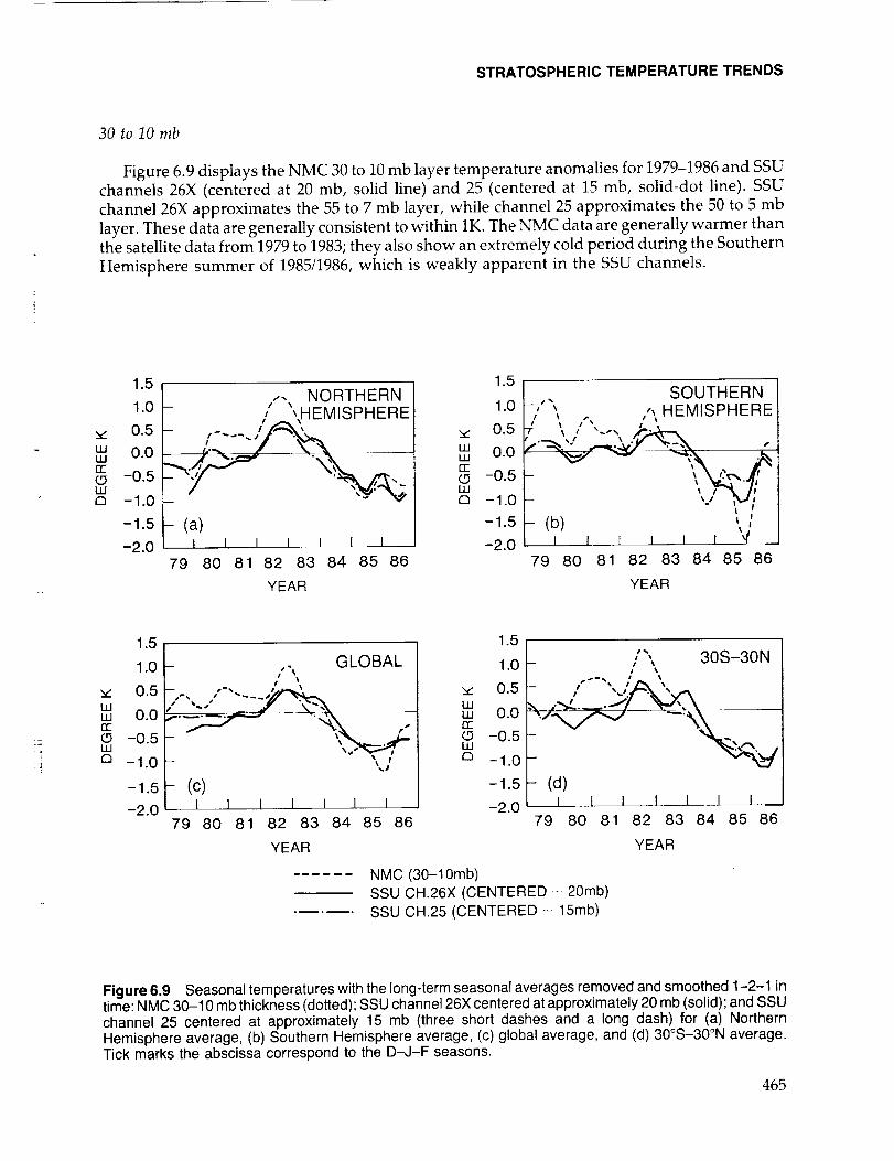
Figure 6.9 displays the NMC 30 to 10 mb layer temperature anomalies for 1979-1986 and SSUchannels 26X (centered at 20 mb, solid line) and 25 (centered at 15 mb, solid-dot line). SSU
channel 26X approximates the 55 to 7 mb layer, while channel 25 approximates the 50 to 5 mb
layer. These data are generally consistent to within 1K. The NMC data are generally warmer thanthe satellite data from 1979 to 1983; they also show an extremely cold period during the Southern
Hemisphere summer of 1985/1986, which is weakly apparent in the SSU channels.
1.5
1.0
,,,. 0.5w 0.0iiin'-
-0.5LUo -1.0
-1.5
-2.0
,-, NORTHERN
,/ ",HEMISPHERE
_ " ,,_
- (a)I I I I I I I
79 80 81 82 83 84 85 86
YEAR
,,¢,
Ww££(.9wO
1.5
1.0
0.5
0.0
-0.5
-1.0
-1.5
-2.0
SOUTHERN' _ ,, HEMISPHERE
/ \ /,, / ,,
.,_,RGI ,.
- \ X,d-".*',.I'\ ]I I
- (b) ',,
79 80 81 82 83 84 85 86
YEAR
1.5
1.0
,,- 0.5ww 0.0n-(.9 -0.5uJ
o -1.0
-1.5
-2.0
f GLOBAL
79 BO B1 g2 g3 84 B5 86
YEAR
N,"
LUWn"(.9W£3
1.5
1.0 L /", 30S-30N/ ... / _
0.5 / " ' '
0.0 • .w. _-1.5[- (dl)-2.0 1 I I I __
79 80 81 82 83 84 85 86
YEAR
NMC (30-10mb)SSU CH.26X (CENTERED --- 20mb)SSU CH.25 (CENTERED -- 15mb)
Figure 6.9 Seasonal temperatures with the long-term seasonal averages removed and smoothed 1-2-1 intime: NMC 30-10 mb thickness (dotted); SSU channel 26X centered at approximately 20 mb (solid); and SSUchannel 25 centered at approximately 15 mb (three short dashes and a long dash) for (a) NorthernHemisphere average, (b) Southern Hemisphere average, (c) global average, and (d) 30°S-30°N average.Tick marks the abscissa correspond to the D-J-F seasons.
465
STRATOSPHERIC TEMPERATURE TRENDS
10 to 5 mb
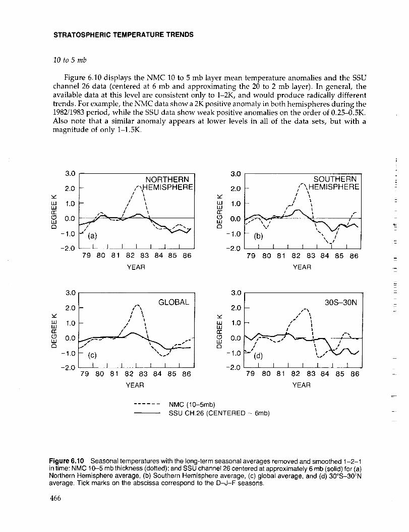
Figure 6.10 displays the NMC 10 to 5 mb layer mean temperature anomalies and the SSU
channel 26 data (centered at 6 mb and approximating the 20 to 2 mb layer). In general, the
available data at this level are consistent only to 1-2K, and would produce radically different
trends. For example, the NMC data show a 2K positive anomaly in both hemispheres during the
1982/1983 period, while the SSU data show weak positive anomalies on the order of 0.25--0.5K.
Also note that a similar anomaly appears at lower levels in all of the data sets, but with a
magnitude of only 1-1.5K.
3.0 3.0
2.0,y,
LU 1.0I..Urr
0.0E3
-1.0
-2.0
3.0
2.0,,¢,
LU 1.0UJcr
0.0LLI£3
-1.0
NORTHERN
- /',_HEMISPHERE1
-- / I
./(a)
l I I t 1 I I
79 80 81 82 83 84 85 86
YEAR
2.0
uJ 1.0LUn"
(.9 0.0U.l£3
-1.0
-2.0
3.0
f SOUTHERN
/'\HEMISPHERE/
79 80 81 82 83 84 85 86
YEAR
- (c)I
79 80
GLOBAL
II I
/t I
I 1 I 1 I 181 82 83 84 85 86
2.0',t"
LU 1.0ILlrr
(.9 0.0IJJ£3
-1.0
-2.0 -2.0
30S-30NI"X
J IJ t
s II I
,/,__t... _. ,ac'/-k.,_(d) L..'v v
I I I I I 1 I79 80 81 82 83 84 85 86
YEAR YEAR
NMC (10-5mb)SSU CH.26 (CENTERED _ 6mb)
=
=
Figure 6.10 Seasonal temperatures with the long-term seasonal averages removed and smoothed 1-2-1in time: NMC 10-5 mb thickness (dotted); and SSU channel 26 centered at approximately 6 mb (solid) for (a)Northern Hemisphere average, (b) Southern Hemisphere average, (c) global average, and (d) 30°S-30°Naverage. Tick marks on the abscissa correspond to the D-J-F seasons.
466

STRATOSPHERIC TEMPERATURE TRENDS
5 to 1 mb
Figure 6.11 displays the NMC 5 to I mb layer mean temperature anomalies with SSU channel
27 (centered at 2 mb and approximating the 5.7 to 0.5 mb layer, solid line) and 36X (centered at 1.5
mb and approximating the 4 to 0.5 mb layer, solid-dot line) brightness temperature anomalies.
Again, the NMC data show a strong positive anomaly between 1982 and 1983 that is not evident
in the satellite data. The SSU data are very consistent with one another. Except for the 1982/1983
period, the data are generally consistent to within 1K of one another, and show a cooling of 1-2Kbetween 1979 and 1986.
uJUJor"
(.9IJJ£3
1.5
1.0
0.5
0.0
-0.5
-1.0
-1.5
-2.0
- ,,"'-,
-lal_ I I I I I t 1
79 80 81 82 83 84 85 86
YEAR
,,¢,
U.IIJJcr(.9LM£3
1.5
1.0
0.5
0.0
-0.5
-1.0
-1.5
-2.0
/", SOUTHERN
_,, /_. "',HEMISPHERE
- (b) \_.'I I I I 1 1 I
79 80 81 82 83 84 85 86
YEAR
',t
LMILlIT"(.9UJ£3
1.5
1.0
0.5
0.0
-0.5
-1.0
-1.5
-2.0
GLOBAL
_-_"-:'.--: . . . \
-- (c) "";
I I I I I I I
79 80 81 82 83 84 85 86
YEAR
UJLIJr'r(.9ILl£3
1.5
1.0
0.5
0.0
-0.5
-1.0
-1.5
-2.0
_, ; 30S-30N• "'_. J_%,_,. F'
_ \./ _I --
- (d) , .---"I I 1 I 1 I I
79 80 81 82 83 84 85 86
YEAR
NMC (5-1 mb)SSU CH.27 (CENTERED - 2mb)SSU CH.36X (CENTERED - 1.5rob)
Figure 6.11 Seasonal temperatures with the long-term seasonal averages removed and smoothed 1-2-1in time: NMC 5-1 mb thickness (dotted); SSU channel 27 centered at approximately 2 mb (solid); and SSUchannel 36X centered at approximately 1.5 mb (solid-dot) for (a) Northern Hemisphere average, (b)Southern Hemisphere average, (c) global average, and (d) 30°S-30°N average. Tick marks on the abscissacorrespond to the D-J-F seasons.
467

STRATOSPHERIC TEMPERATURE TRENDS
0.5 mb
Figures 6.12a-d display the SSU channel 47X data centered at 0.5 mb and approximating the1.2 to 0.2 mb layer. Few reliable data were available for comparison at this level, with the
exception of the irregularly spaced rocketsonde data (see the following discussion). These datashow an almost linear cooling of 2.5K from late 1979 to late 1986. Nash and Forrester (1986)
estimate this channel to have a standard error of about 1K because of the sensitivity to changes in
SSU channel 27's spectroscopic performance.
In addition to these conventional data sets, the data have also been compared to the
rocketsondes (see Section 6.2.3). These rocketsonde data are irregularly spaced and are con-
centrated primarily in the Northern Hemisphere, with the exception of Ascension Island at 9°S,
14°W. Figures 6.13-16 display comparisons of rocketsonde and zonal mean satellite data fromthree stations at four different levels. These three stations (Ascension Island, 9°S to 14°W; Cape
Canaveral, 28°N to 81°W; and Kwajalein Island, 9°N to 168°E) were chosen for the length and
continuity of their data over 1979 to 1986.
h_
U3I.Urv(9tU£3
1.5
1.0
0.5
0.0
-0.5
-1.0
-1.5
-2.0
NORTHERN
- _x_ HEMISPHERE
(a) "k"/--%
t t I t 1 1 I
79 80 81 82 83 84 85 86
YEAR
ILlIIIrr(9UJ£3
1.5
1.0
0.5
0.0
-0.5
-1.0
-1.5
-2.0
SOUTHERN
I J 1 1 I t 1
79 80 81 82 83 84 85 86
YEAR
1.5
1.0
,,," 0.5
0.0
-0.5
-1.0
-1.5
-2.0
1.5
_ GLOBAL 1.o
v 0.5
0.0
_ -0.5
_ -1.0
-1.5
I I I I I I I -2.079 80 81 82 83 84 85 86
_ 30S-30N
Y, I 179 80 81 82 83 84 85 86
YEAR YEAR
SSU CH.47X (CENTERED - 0.5mb)
Figure 6.12 Seasonal temperatures with the long-term seasonal averages removed and smoothed 1-2-1in time for SSU channel 47X centered at approximately 0.5 mb for (a) Northern Hemisphere average, (b)Southern Hemisphere average, (c) global average, and (d) 30°S-30°N average. Tick marks on the abscissacorrespond to the D-J-F seasons.
468

STRATOSPHERIC TEMPERATURE TRENDS
Figures 6.13a-c display rocket data averaged from 27.5 km to 37.5 km in comparison to the
SSU channel 25 zonal mean data. SSU channel 25 is centered at 15 mb (-30 km), with a weightingfunction width of about 17 km. The Cape Canaveral data are compared to the 30°N SSU zonal
mean; the Ascension data are compared to the 10°S SSU data; and the Kwajalein data are
compared to the 10°N SSU data. The rocketsonde data are processed by finding the deviation
from the long-term monthly mean, interpolating missing months, averaging the deviations into
seasons, and, finally, smoothing the seasonal deviations with a 1-2-1 filter. In general, the data
on these plots are consistent to only 1-2K. This poor consistency could result from the com-
pariso_n of single station data to the satellite data zonal means. For example, all three rocket data
sets show a strong quasi-biennial oscillation (QBO) signal that is largely absent from the SSU data
at 10°S (Figure 6.13a) and 10°N (Figure 6.13c). A visual averaging of Kwajalein and Ascension
shows that two large minima would still appear at the tick marks between 80/81 and 82/83--QBO
minima at both stations. Nastrom and Belmont (1975) showed that the QBO has a 2K amplitude
and is vertically deep (-20 km) in the region of SSU channel 25's weighting function; thus, this
channel should have peak anomalies in excess of 1K. It is not clear why SSU channel 25 cannotresolve the QBO.
v
WuJrv
Wa
3.0
2.0
1.0
0.0
-1.0
-2.0
-- p% e'L
.i ,,, ,"'TJ,-A.,'-' "
ASCENSION ISLAND- (a) 9S 14W
1 I 1 I I I ....1
79 80 81 82 83 84 85 86
YEAR
3.0
2.0
LU 1.0UJn-
(.9 0.0LU
-1.0
-2.0
t '", CAPE
I i!, \ CANAVERAL!, \ 28N 81W
"F "_ JJ I ! I ! % %.....-- % 1
(b) ",, ,-
] I I I 1 I I
79 80 81 82 83 84 85 86
YEAR
I.IJUJrr(.9ILl£3
3.0
2.0
1.0
0.0
-1.0
-2.0
KWAJALEIN9N 168E
%#
- (c)I I I I I T I
79 80 81 82 83 84 85 86
YEAR
SSU CH.25 (CENTERED - 15mb)ROCKET 30-35km AVG.
Figure 6.13 Seasonal temperatures with the long-term seasonal averages removed and smoothed 1-2-1in time for the 30-35 km layer average of station rocket data (dotted) and the corresponding zonal average ofSSU channel 25 centered at approximately 15 mb (solid) for (a) Ascension Island (9°S, 14°W), (b) CapeCanaveral (28°N, 81°W), and (c) Kwajalein (9°N, 168°E). Tick marks on the abscissa correspond to the D-J-Fseasons.
469
STRATOSPHERIC TEMPERATURE TRENDS
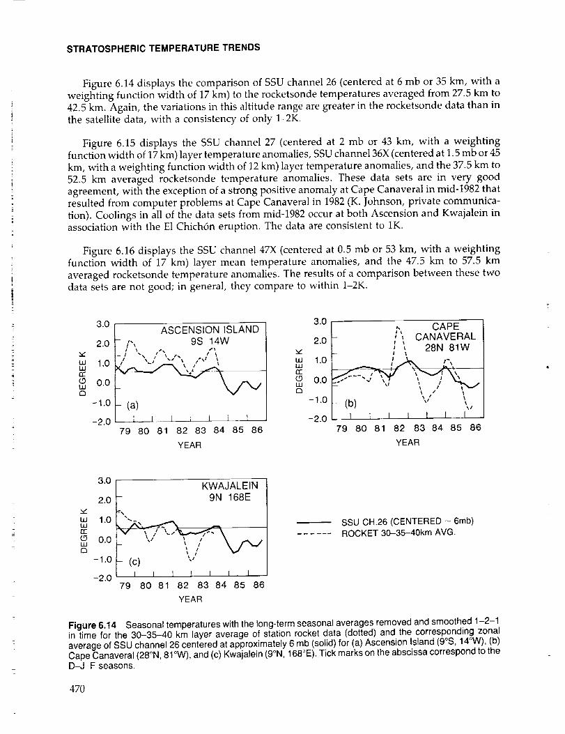
Figure 6.14 displays the comparison of SSU channel 26 (centered at 6 mb or 35 km, with a
weighting function width of 17 km) to the rocketsonde temperatures averaged from 27.5 km to
42.5 km. Again, the variations in this altitude range are greater in the rocketsonde data than inthe satellite data, with a consistency of only 1-2K.
Figure 6.15 displays the SSU channel 27 (centered at 2 mb or 43 km, with a weightingfunction width of 17 km) layer temperature anomalies, SSU channel 36X (centered at 1.5 mb or 45
km, with a weighting function width of 12 km) layer temperature anomalies, and the 37.5 km to52.5 km averaged rocketsonde temperature anomalies. These data sets are in very good
agreement, with the exception of a strong positive anomaly at Cape Canaveral in mid-1982 that
resulted from computer problems at Cape Canaveral in 1982 (K. Johnson, private communica-
tion). Coolings in all of the data sets from mid-1982 occur at both Ascension and Kwajalein in
association with the E1 Chich6n eruption. The data are consistent to 1K.
Figure 6.16 displays the SSU channel 47X (centered at 0.5 mb or 53 km, with a weightingfunction width of 17 kin) layer mean temperature anomalies, and the 47.5 km to 57.5 km
averaged rocketsonde temperature anomalies. The results of a comparison between these two
data sets are not good; in general, they compare to within 1-2K.
,./
WuJIT(.9uJQ
3.0
2.0
1.0
0.0
-1.0
-2.0
ASCENSION ISLAND- ,,, 9S 14W/,--,1 ",, /' '.,'" .,/
- (a)! I L L I t I
79 80 81 82 83 84 85 86
YEAR
3.0
2.0
uJ 1.0uJi-r
0.0uJD
-1.0
-2.0
i, CAPE- , _ CANAVERAL
i _ 28N 81W
- \ , \(b) "" '
1 L t t 1 I I
79 80 81 82 83 84 85 86
YEAR
3.0
2.0f KWAJALEIN
9N 168E
79 80 81 82 83 84 85 86
,y,
tu 1.0LUIT"
0.0LLI£3
-1.0
-2.0
SSU CH.26 (CENTERED - 6mb)ROCKET 30-35-40km AVG.
YEAR
Figure 6.14 Seasonal temperatures with the long-term seasonal averages removed and smoothed 1-2-1in time for the 30-35-40 km layer average of station rocket data (dotted) and the corresponding zonalaverage of SSU channel 26 centered at approximately 6 mb (solid) for (a) Ascension Island (9°S, 14°W), (b)Cape Canaveral (28°N, 81°W), and (c) Kwajalein (9°N, 168°E). Tick marks on the abscissa correspond to theD-J-F seasons.
470

STRATOSPHERIC TEMPERATURE TRENDS
hCLULUCE(.9UJn
3.0
2.0
1.0
0.0
-1.0
-2.0
ASCENSION ISLAND- 9S 14W
(a)I I t_. L I I I
79 80 81 82 83 84 85 86
uJLU£E(.9LU
3.0
2.0
1.0
0.0
--1.0
-2.0
CAPE_'_, CANAVERAL' ' 28N 81W
_.._, • _ , _ I
- (b) _"--_g.,,I, _ _ _______t__L_x_._
79 80 81 82 83 84 85 86
YEAR
3.0
2.0
Lu 1.0ILlrr
o 0.0uJ£3
-I.0
-2.0
KWAJALEIN9N 168E
Ic) 'v' ",,__ I I I I 1 I
79 80 81 82 83 84 85 86
YEAR
SSU CH.27 (CENTERED - 2mb)
SSU CH.36X (CENTERED --- 1.5mb)
ROCKET 40-.45-50km AVG.
Figure 6.15 Seasonal temperatures with the long-term seasonal averages removed and smoothed 1-2-1in time for the 40-45-50 km layer average of station rocket data (dotted) and the corresponding zonalaverage of SSU channel 27 centered at approximately 2 mb (solid) and SSU channel 36X centered atapproximately 1.5 mb (solid-dot) for (a) Ascension Island (9°S, 14°W), (b) Cape Canaveral (28°N, 81 °W), and(c) Kwajalein (9°N, 168°E). Tick marks on the abscissa correspond to the D-J-F seasons.
I.UILlCr(-9LUO
3.0
2.0
1.0
0.0
-1.0
--2.0
ASCENSION ISLAND9S 14W
% I , /-_ i i
(a)I I I I I I I
79 80 81 82 83 84 85 86
YEAR
u.ln'-
w0
3.0
2.0
1.0
0.0
-1.0
-2.0
,fi, _ CAPE
: _ CANAVERAL
,; ',, 28N 81W
(b) - "", '_,_ I I I I l ._[_
79 80 81 82 83 84 85 86
YEAR
3.0 __ KWAJALEIN2.0 9N 168E
_u 1.0 / ', ,'_
CC
_3 0.0 \uJo "',/ \
-1.0
-2.0 / I I I I 1 l I
79 80 81 82 83 84 85 86
YEAR
SSU CH.47X (CENTERED _ 0.5mb)
...... ROCKET 50-55km AVG.
Figure 6.16 Seasonal temperatures with the long-term seasonal averages removed and smoothed 1-2-1in time for the 50-55 km layer average of station rocket data (dotted) and the corresponding zonal average ofSSU channel 47X centered at approximately 0.5 mb (solid) for (a) Ascension Island (9°S, 14°W), (b) CapeCanaveral (28°N, 81°W), and (c) Kwajalein (9°N, 168°E). Tick marks on the abscissa correspond to the D-J-Fseasons.
471
STRATOSPHERIC TEMPERATURE TRENDS
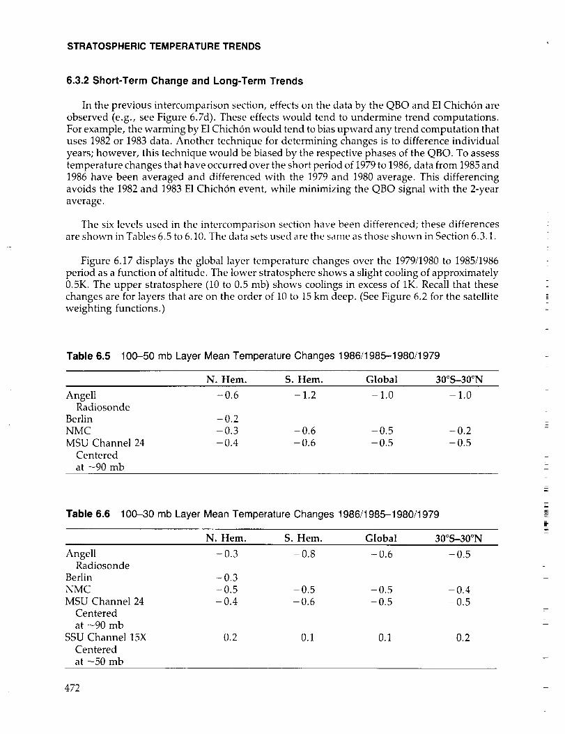
6.3.2 Short-Term Change and Long-Term Trends
In the previous intercomparison section, effects on the data by the QBO and E1 Chich6n are
observed (e.g., see Figure 6.7d). These effects would tend to undermine trend computations.
For example, the warming by E1 Chich6n would tend to bias upward any trend computation that
uses 1982 or 1983 data. Another technique for determining changes is to difference individual
years; however, this technique would be biased by the respective phases of the QBO. To assess
temperature changes that have occurred over the short period of 1979 to 1986, data from 1985 and
1986 have been averaged and differenced with the 1979 and 1980 average. This differencing
avoids the 1982 and 1983 E1 Chich6n event, while minimizing the QBO signal with the 2-year
average.
The six levels used in the intercomparison section have been differenced; these differencesare shown in Tables 6.5 to 6.10. The data sets used are the same as those shown in Section 6.3.1.
Figure 6.17 displays the global layer temperature changes over the 1979/1980 to 1985/1986
period as a function of altitude. The lower stratosphere shows a slight cooling of approximately
0.5K. The upper stratosphere (10 to 0.5 rob) shows coolings in excess of 1K. Recall that thesechanges are for layers that are on the order of 10 to 15 km deep. (See Figure 6.2 for the satellite
weighting functions.)
Table 6.5 100-50 mb Layer Mean Temperature Changes 1986/1985-1980/1979%
N. Hem. S. Hem. Global 30°S-30°N
Angell -0.6 - 1.2 - 1.0 - 1.0Radiosonde
Berlin - 0.2
NMC -0.3 -0.6 -0.5 -0.2MSU Channel 24 -0.4 -0.6 -0.5 -0.5
Centeredat -90 mb
Table 6.6 100-30 mb Layer Mean Temperature Changes 1986/1985-1980/1979
N. Hem. S. Hem. Global 30°S-30°N
Angell - 0.3 - 0.8 - 0.6 - 0.5Radiosonde
Berlin - 0.3
NMC -0.5 -0.5 -0.5 -0.4
MSU Channel 24 - 0.4 - 0.6 - 0.5 - 0.5Centered
at -90 mb
SSU Channel 15X 0.2 0.1 0.1 0.2
Centered
at -50 mb
472

T_
STRATOSPHERIC TEMPERATURE TRENDS
Table 6.7 30-10 mb Layer Mean Temperature Changes 1986/1985-1980/1979
N. Hem. S. Hem. Global 30°S-30°N
NMC - 0.6
SSU Channel 26X -0.3
Centeredat -20 mb 1
SSU Channel 25 -0.6
Centered
at -15 mbAscension Is. 2 30 km
(9°S, 14°W)
Cape Canaveral 3 30 km
(28°N, 81°W)
Kwajalein 4 30 km
(9°N, 168°E)
-1.4 -1.0 -1.0
-0.6 -0.5 -0.8
-0.6 -0.6 -0.9
0.1
-0.7
-0.1
1The first period is the 2-year average September 1979-August 1981.2The second period is the 2-year average August 1982-July 1984.3The second period is the 2-year average September 1984-August 1986.4The second period is the 2-year average July 1982-June 1984.
Table 6.8 10-5 mb Layer Mean Temperature Changes 1986/1985-1980/1979
N. Hem. S. Hem. Global 30°S-30°N
NMC - 0.3
SSU Channel 26 -0.6
Centered
at -6 mb
Ascension Is.' 35 km
(9°S, 14°W)
Cape Canaveral 2 35 km
(28°N, 81°W)
Kwajalein 3 35 km
(9°N, 168°E)
-0.2 -0.2 +0.3
-0.6 -0.6 -1.0
-0.1
-0.1
-1.3
_The second period is the 2-year averageZThe second period is the 2-year average3The second period is the 2-year average
August 1982-July 1984.September 1984-August 1986.July 1982-June 1984.
Figure 6.18 displays the 30°S to 30°N layer temperature changes over the 1979/1980 average
to 1985/1986 average period as a function of altitude. Three rocketsonde stations (Ascension
Island, Cape Canaveral, and Kwajalein Island) are also included on this figure. Again, as inFigure 6.17, a small cooling is seen in the lower stratosphere, and a cooling of 1-2K in the
upper stratosphere. The rocketsonde data tend to bracket the satellite data, thus illustrating the
need for zonal averaging and showing that caution is needed when analyzing for trends at singlestations.
The error bars used in Figures 6.17 and 6.18 are taken from the discussion in Section 6.2. The
satellite data monthly zonal mean rms error is 0.2K (1K for synthesized channels), the daily
473

STRATOSPHERIC TEMPERATURE TRENDS
Table 6.9 5-1 mb Layer Mean Temperature Changes 1986/1985-1980/1979
N. Hem. S. Hem. Global 30°S-30°N
NMC - 1.4
SSU Channel 27 -1.3
Centeredat -2 mb 1
SSU Channel 36X -1.4
Centeredat -1.5 mb
Ascension Is. 2 40 km
(9°S, 14°W) 45 km
Cape Canaveral 3 40 km
(28°N, 81°W) 45 kmKwajalein 4 40 km
(9°N, 168°E) 45 km
-1.5 -1.4 -2.8-1.2 -1.2 -1.5
-1.4 -1.4 -1.7
-0.7
-1.2
-0.3
-0.5-2.5
-2.5
1The first period is the 2-year average September 1979-August 1981.
2The second period is the 2-year average August 1982-July 1984.
_The second period is the 2-year average September 1984_August 1986.
4The second period is the 2-year average July 1982-June 1984.
Table 6.10 0.5 mb Layer Mean Temperature Changes 1986/1985-1979/1980
N. Hem. S. Hem.
SSU Channel 47X - 2.1
Centeredat -0.5 mb 1
Ascension Is. 2 50 km
(9°S, 14°W) 55 km
Cape Canaveral 3 50 km
(28°N, 81°W) 55 km
Kwajalein 4 50 km
(9°N, 168°E) 55 km
Global
-1.7-1.4
30°S-30°N
-1.3
-0.6
0.4
-2.0
-2.3-1.2
-1.0
z
1The first period is the 2-year average September 1979-August 1981.
2The second period is the 2-year average August 1982-July 1984.
-_Fhe second period is the 2-year average September 1984-August 1986.
4The second period is the 2-year average July 1982-June 1984.
radiosonde based data should have errors on the order of 0.5K (based on the reproducibility of
measurements; see Figure 6.1), the daily rocketsonde data have a repeatability of 0.8K (35 km) to1.3K (50 km), and the NMC data errors are estimated from the daily radiosonde errors (0.5K in
lower stratosphere) and daily rocketsonde errors (1.3K in the upper stratosphere). Monthlyaveraging should reduce the random errors in these data; hence, the error estimates for the
rocket, radiosonde, and NMC data are very conservative. NMC errors are 1.5K at the upperlevels.
The only data sets available for the longer term stratospheric trends are the Angell andKorshover (AK) radiosonde data, the Berlin data (B), and the rocketsonde data (R). The AK and B
data (lower stratosphere) have been available only since 1970 and 1962, respectively. The R data
(upper stratosphere and lower mesosphere) have limited spatial coverage.
4742

STRATOSPHERIC TEMPERATURE TRENDS
GLOBAL TEMPERATURE CHANGES
E
Wn"
0309LUn"EL
0.4
3
10-
30-
100 -
f t
I-_-.- 4 7 X -_.-_
t--_ 36X _
27I--_ NMC---_----_
I_-._---- NM(
25I------_NMC -_1
_-------26 X--
26
- 56
48
4oW
F-32 -J
<
24
-15X-_-.-I
_AR-_
I I i___ _R__4--_--NMC ' 16-3 -2 -1 0 1 2
TEMPERATURE CHANGE(K)
Figure 6.17 Summary of global stratospheric temperature differences (1985 and 1986 minus the averageof 1979 and 1980). Symbols denote Angell's radiosonde data (AR), NMC data (NMC), and satellite data
(channel numbers, see Figure 6.2). Error bars denote uncertainties (see text). Nash and Forrester (1986)
estimate their satellite errors as 0.2 K rms (1 K rms for synthesized channels).
EQUATORIAL TEMPERATURE CHANGES
04
g 3LUn"
LUn- 10Q_
3O
100--z
-I I CC I ii iKI"
47X
_- AI --1. KI_
i CC
36XKI _'t==L---_ CC --
27NMC
' AI I 4_1
26________ ATNMC
P-._- tG ._..-I
CC -- "_AI
NMC25._
26X -- .--4
p- NMC'7
¢'--- AR ___ NMC --_
56
48
4oWO
32 _,
24
1 t 24 I 16-3 -2 -1 0 1 2
TEMPERATURE CHANGE (K)
Figure 6.18 As in 6.17, except for Tropics and including rocket stations. Kwajalein Island (KI; 9°N, 168°E),
Ascension Island (AI; 9°S, 14°W), and Cape Canaveral (CC; 28°N, 81°W).
475
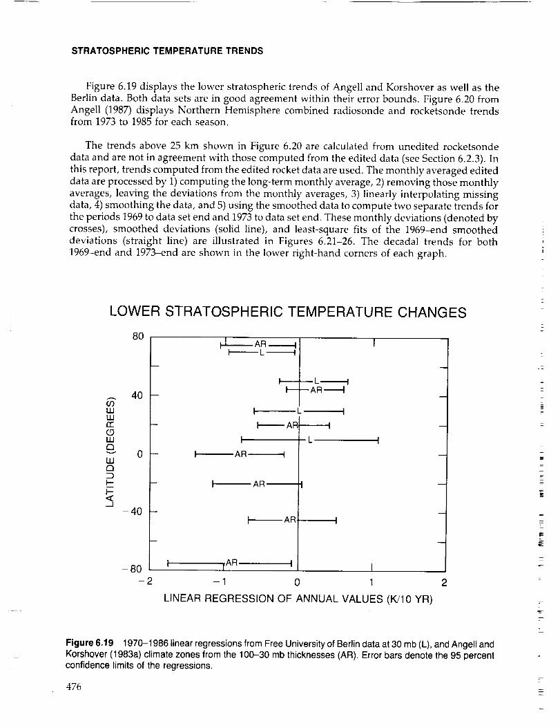
STRATOSPHERIC TEMPERATURE TRENDS
Figure 6.19 displays the lower stratospheric trends of Angell and Korshover as well as the
Berlin data. Both data sets are in good agreement within their error bounds. Figure 6.20 fromAngeI1 (1987) displays Northern Hemisphere combined radiosonde and rocketsonde trendsfrom 1973 to 1985 for each season.
The trends above 25 km shown in Figure 6.20 are calculated from unedited rocketsonde
data and are not in agreement with those computed from the edited data (see Section 6.2.3). In
this report, trends computed from the edited rocket data are used. The monthly averaged edited
data are processed by 1) computing the long-term monthly average, 2) removing those monthly
averages, leaving the deviations from the monthly averages, 3) linearly interpolating missingdata, 4) smoothing the data, and 5) using the smoothed data to compute two separate trends for
the periods 1969 to data set end and 1973 to data set end. These monthly deviations (denoted by
crosses), smoothed deviations (solid line), and least-square fits of the 1969-end smoothed
deviations (straight line) are illustrated in Figures 6.21-26. The decadal trends for both
1969-end and 1973-end are shown in the lower right-hand corners of each graph.
LOWER STRATOSPHERIC TEMPERATURE CHANGES
oowwor"(.9UJ£3
WI"7
<_J
80
4O
-40 -
-80-2
}..L.._ AR --tI_------ L -_--!
I L I
I--_AR
I
I AR I
I AR •
I AR
L t
1 IAR ! I
--1 0 1
LINEAR REGRESSION OF ANNUAL VALUES (K/10 YR)
2
Figure 6.19 1970-1986 linear regressions from Free University of Berlin data at 30 mb (L), and Angell andKorshover (1983a) climate zones from the 100-30 mb thicknesses (AR). Error bars denote the 95 percentconfidence limits of the regressions.
476
z
_=
=
=
=

STRATOSPHERIC TEMPERATURE TRENDS
SEASONAL CHANGES IN TEMPERATURE
rr>-
o
(.3ov
LLI(.9Z<-'r-0
LLICC
I--<rTLLI13..
iiiI.--
1
0
-1
-2
-3
-4
1
0
-1
-2
-3
1
0
-1
-2
1
0
-1
1
0
-1
I 1 I46-55 km
D
i I
m
m
m
36-45 km
..
l
B
26-35 km
16-24 km
i
m
m
9-16 km
1
0
1
0
-1
I _ ]: -[ _ 1.5-9 kmi i i •
I _ SURFACE1" j. j
I I I
DJF JJA DJF
Figure 6.20 Seasonal changes in tropospheric and stratospheric Northern Hemisphere temperature
(degrees Celsius per 10 years) between 1973 and 1985 (DJF is December-January- February, etc.) basedon linear regression applied to rocketsonde data primarily in the Western Hemisphere (values above 25 km)
and radiosonde data around the entire hemisphere. The vertical bars are 95 percent confidence limits for the
seasonal changes, as estimated from the standard deviation of seasonal temperatures about the line of
regression.
477
STRATOSPHERIC TEMPERATURE TRENDS
Ascension Island (8°S)
Figure 6.21 depicts the monthly data and the trend for each of the six levels at Ascension
Island. The trends observed at 30, 35, and 40 kilometers are large and positive. The trend is about
-0.1K per decade at 50 km and - 1.0K per decade at 55 km over 1973-1985. The QBO signal isseen in the data, with an amplitude of about 2K.
KwajaIein, Marshall Islands (9°N)
The Kwajalein data show evidence of the QBO signal at altitudes below 45 km with an
amplitude of I to 2K. The 1973-1985 temperature trends for Kwajalein are small, as seen in Figure
6.22. At 30 km, the trend is only 0.7K per decade, while at 35 km to 55 km, the trends are evensmaller.
Barking Sands, Hawaii (22°N)
The 1973-1982 trends calculated for Barking Sands also are small. Figure 6.23 shows that the
rate of temperature decrease is, at 30 km, 0.8K per decade; at 35 km, - 0.6K per decade; at 40 km,
0.3K per decade; and at 45 and 50 km, 0.3K and 1.9K per decade, respectively. At 55 km, the rate
of increase is larger: 1.0K per decade. The temporal temperature structure at Barking Sandsshows the QBO with a 1 to 2K amplitude.
Cape Canaveral, Florida (28°N)
Weak downward trends from 1973-1985 are noted at all altitudes, with the exception of 55
km. For example, Figure 6.24 shows downward temperature trends of - 0.2K per decade at 30
kin, -0.6K per decade at 35 km, - 1.0K per decade at 40 km, -0.7K per decade at 45 km, and
-0.6K per decade at 50 km. The QBO is again clearly seen, with an amplitude of 1-3K.
Pt. Mugu, California (34°N)
The Pt. Mugu 1973-1982 temperature trends (Figure 6.25) vary between no trend at 35 km to a
2.3K per decade trend at 55 km. A weaker (1K amplitude), chaotic QBO signal is apparent at 30km.
Primrose Lake, Canada (55°N)
Temperature trends from 1973-1985 at Primrose Lake are shown in Figure 6.26. The regres-
sion analysis, however, indicates downward as well as upward trends at the different altitudes.
These varying trends may be a result of the large interannual variability in high latitudes
combined with the missing data. For example, at 30 km, the trend is indicated as 1.5K perdecade, while at 35 km it appears to be upward at a rate of 2.5K per decade. Essentially, the
trends calculated for the Primrose Lake temperature data may be inconclusive because of the
aforementioned large interannual variability and missing monthly average data.
The six rocketsonde sites show downward temperature trends in the stratosphere when the
1969, 1970, and 1971 data are included in the trend analysis. Since rocketsonde sites are uniquely
located and few in number, it is impossible to determine a zonal or global trend from these data.
There is still disagreement between researchers over differences in the rocketsonde data during
the 1970-1972 period.
478
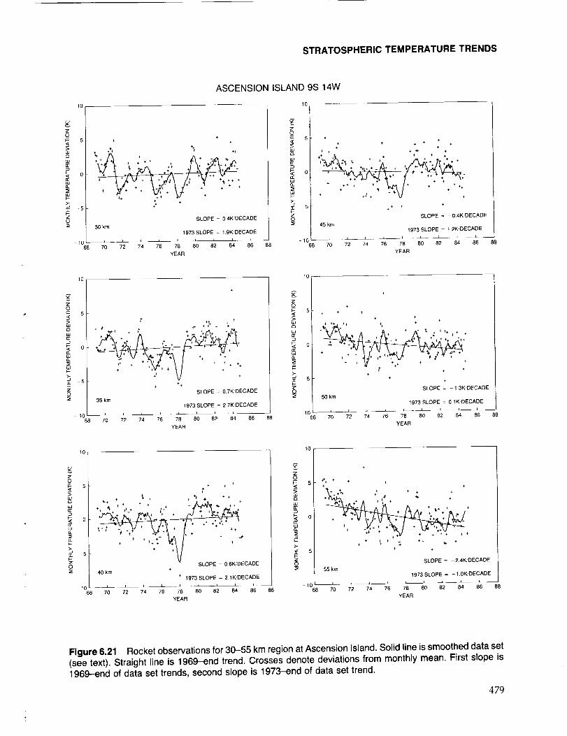
STRATOSPHERIC TEMPERATURE TRENDS
,,>,
o_
0
ASCENSION ISLAND 9S 14W
10
5 • ÷4-
+ + ÷ ___
++ + ++ + + + + + + ++
÷ ÷+ + + + + +
0 _ + + + +
+
÷ + + + +÷ + + ÷ +
+*
SLOPE 0.4K_DECADE
30 km
1973 SLOPE 1.9K/DECADE
10 ........ 8_--- 86_868 70 72 74 76 78 80 82 8
YEAR
5
Zo_
_:>
(3_
,,=,F-
>-
£- s}-
5 ÷4.
+ + + ._ +÷ + + ++ +
÷÷ + ÷ + + +
÷ **_ _. ,- ÷ ,*** ++ ++ + ÷,_+ 4. + 4. + + + +
+ 4. _4. ++
+_++÷ ++ 4. ÷ + ÷+
+ ÷ ++
SLOPE = -0,4KDECADE
45 krn
1973 SLOPE = 1 2K,,'DECADE
1068 70 72 74 76 78 80 82 84 86
YEAR
88
>=E)
o=<
-s
10
68
_++ , ÷ ÷ ++ 4. *+ + + + +
4. ,.+4.. *3, ÷ *
2' ", ";4.-+
+ ÷+
SLOPE - 0.7K/DECADE
35 km
1973 SLOPE 27K/DECADE
8670 72 74 76 78 80 82 84
YEAR
10
Z
_o
oo.
:r 5
0
-1088 68 88
+ * 4-
+ ++ ++ _+ 4. ÷ +
÷+ +
+_t* *_÷4.,÷,, ÷ **4. ÷÷4. ++**
_ _. ÷4.
++
SLOPE = 1.3K DECADE
50 km
1973 SLOPE = 0.1K..'DECADE
70 72 74 76 78 80 82 84 86
YEAR
I0
5
0
5
_+ + + + 4.
% *_, 4.÷+4. ;+__. + ÷
+ ÷ ++
÷ +
÷+ ÷
t_ + +
+ % ++4.
++÷
÷ _,-+
SLOPE 0 6K, DECADE
40 km
+ 1973 SLOPE = 2.1K/DECADE
10 ......... 84-- 8668 70 72 74 76 78 80 82 88
YEAR
Z_o
>
II-
10
5
÷
5 #** + +÷ ÷
***_ 2 ÷ ÷ *
÷_.^÷4. I_ ÷_ 4. "* "
++ ÷ + ++ + _ +
+ +
+
+ + + + 4.+ +÷ + + +_
+ +
SLOPE = -2.4K/DECADE
55 km
1973 SLOPE = - 1.0K/DECADE
1068 70 72 74 76 80 82 84 8
YEAR
Figure 6.21 Rocket observations for 30-55 km region at Ascension Island. Solid line is smoothed data set(see text). Straight line is 1969-end trend. Crosses denote deviations from monthly mean. First slope is1969-end of data set trends, second slope is 1973-end of data set trend.
479

STRATOSPHERIC TEMPERATURE TRENDS
5
oIi
>-s
.<
5£3
==
ell
v
5<
_- o
>-,
KWAJALEIN ISLAND 9N 168E
++
,÷ + ÷ ++
+ ++ + # + + _ +
+ +_+ +
+ + + _+ +
+
SLOPE 06KDECADE
30 km
1973 SLOPE 0 7KOECADE
lO , _ _ , _ , , , _--_68 70 72 7 76 7 60 82 84 8
YEAR
10
56
_3
h
+++ +
* ++÷#t. + *+ +
+2 +
÷
+ + ÷
SLOPE : 1 7K DECADE
45 km
1973 SLOPE = 0.2KrDECADE
1068___ l /2 I _ I 8=0 I 4" -B'=870 74 76 78 82 8 8
YEAR
10 --
+
÷
+ ++ -_. ++ + +
÷ + +_ + +÷ +
._ + +
+ +. _
÷+5 _
SLOPE 1.6K!DECADE
35 km
1973 SLOPE 0 1K DECADE
10 - _-- J68 70 72 7'4 76 78 60 8_2 8'4 8'6 88
YEAR
£3
ogo_
h"r 5
O
-1068
+
+÷
++÷ + + ÷ +
+ +++ + +. + ++ _# + + +
+ ++ ++
+ ,+ +
÷÷+ ÷
*
SLOPE I9K DECADE
50 km
1973 SLOPE 0,3K DECADE
i , i J _ , f -- 84= 8_670 72 74 76 78 80 82 88
YEAR
10 m
++
+
+ +++ +++
SLOPE 1 8K:DECADE
40 km
1973 SLOPE - 0 2K DECADE
10 .... 7 80 ' ' 2668 70 72 74 76 8 82 84 88
YEAR
Z
_O
£3
#
o£E
h
+
+++ ÷
+ ++ + + ++ + # ++
÷_÷'..÷÷÷A_ + _÷ ,X
÷ ÷ ÷ +_÷ _. ÷ j.
÷ ÷ +
+
SLOPE = - 1.6K DECADE
55 km
1973 SLOPE = 0.1K DECADE
-1o ....... _ , _4 a'668 70 72 74 76 78 8 82 88
YEAR
z
m
z
Figure 6.22 Same as 6.21 except for Kwajalein.
480

STRATOSPHERIC TEMPERATURE TRENDS
BARKING SANDS, 22N 160W
10
v
s;>
g
{:E
p.
:I: 5
EO
-10 i 712 .......... i2 84 r68 70 74 76 78 80 8 86 88
YEAR
+
t?
?_ ++ t
+ + + %. + + + +÷ +÷
+ _ + ++ ÷_+ * + ++ + +
+ + + _+ 4+
+
SLOPE - 1 8K DECADE
30 km
1973 SLOPE = 0 5K DECADE
v
5
>
g
>,:r 5
O
÷÷ ++ ÷
++++ +
*_.._Jy+ ,,,÷ _ + **+ +÷
+ _++ ÷ ++. + + + +
+ +_ +
+* 4- ++ *+4- + _, ,++, +,
+ _+ + +
45 km
SLOPE = 1.8K DECADE
1973 SLOPE : 03KDECADE
'° 7'0 ........ _o ' ' '88 72 74 76 78 82 84 86 88
YEAR
10
5s
>
g
o[E
5
O
+ ++ ÷ ÷
+ _. + +
+ ++ + ÷
+ + ÷ 4.+ ÷ 4. ,+
+ + ,,++ _+
+ + ++ ++ +
SLOPE = 2 3K DECADE35 km
1973 SLOPE : 08KDECADE
t0 i i _ l ; t____ _L _ --
68 70 72 74 76 78 80 82 84 86 98
YEAR
10 ....
__55
>
g
,_ o
Q_
z©
+
% ÷
÷+_+* + + ++ + + +. A+ +
+ ++ ++ *++_ ÷ + +
+ + + ,. ._
+ +* ÷+÷+ . +; ,
+5 *
+ SLOPE 0.9K DECADE50 km
1973 SLOPE 1 9K DECADE
68 70 72 74 76 78 80 82 84 86 88
YEAR
10
85
£3
,_ 0B:
>,3: 5
©
+÷ %*r + +
_+ ++ +
4+ + _+
+ + +
÷ ÷ ÷ + ÷ +++ +
+ * + _, , ,+ + ,+ - + ÷
+
+
SLOPE = 23K DECADE40 km
1973 SLOPE = - 0.6K DECADE
10 I I__ I I I t I I •
68 70 72 74 76 78 80 82 84 86 88
YEAR
gz
R<
0
F-
s
+
÷
++ + + +
•" ± +
+ + ++ + + ÷ + + +
÷+ _. +
+ %.+++ + +
÷+
SLOPE 21K DECADE
55 km
1973 SLOPE 10K DECADE
t068 70 72 7 76 7 0 82 84 86 88
YEAR
Figure 6.23 Same as 6.21 except for Barking Sands.
481
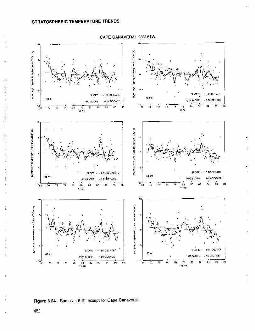
STRATOSPHERIC TEMPERATURE TRENDS
10
CAPE CANAVERAL 28N 81W
10
z
_o6
o
>_,6
zO
+ +
• ÷ + +++ + ÷ +
+ + + + + ,+÷, + ÷ + + ++
+ ++ + ++ + ,_ _.
+ ++_+
+ ++ _- + +
+ +÷
SLOPE = - 1.0K,DECADE
30 km
1973 SLOPE O.2KDECADE
.... 8'0 ' ' ' -_- 1068 70 72 74 76 78 82 84 86 8
YEA R
Z
_o6
>
o
_L
z0
+
+_ + ÷ + +
q , + ÷_. + + +
÷ .._ +_t+ + +÷ + + _A÷,p
+,++ +% + +._ ++ +,++*+
+ _ + ++ _
• ,+ * + +÷ + f_ ÷ + , + +
+
+ ,SLOPE 1.6K DECADE
45 km * +
1973 SLOPE - 0 7K_DECADE
' ;_ _;6 _o " ' '1088 70 82 84 86 86
YEAR
10
Z_o_- 5<
,_ o,,=,0-
0
++ +
+
+\+ +++ ++ ++ + _- + +
++ _- + + +41.
++ + + + + + + + +++ +_ + +
++ + ,
÷ ÷ +
+ + + + +
+SLOPE = - 1.61_'DECAOE +
35 km+
1973 SLOPE == 0 6K DECADE
i i i i ___ i T I J- 1068 70 72 74 76 78 60 62 84 66 88
YEAR
10
6.,>.o
0
Q.
>_,:_ 5
O
÷
+ +
÷ ++ +
+ +,+ ,+ + +++ + * , +
•_ + + ++
, ' _'÷ ÷+÷5+2 + +. +
+ +
+÷
SLOPE" = 09K DECADE
50 km +
1973 SLOPE 0 6K DECADE
---- s I I I
YEAR
10
+
÷+
÷
+ + ÷ *
+ ÷+ +++ + +
÷ _ + ++ + + + % ++_ ÷
+
÷+ _ + _.
+ + +
_2Z_o
5
i SLOPE = - t.6K DECADE + +
+ ÷
40 km
1973 SLOPE = - 1.0K DECADE
1°66 7'o _'_ ,_-_6 ;6 _0 _ 6, _6 8_YEAR
10
5
>
o
o.
5
0
+
÷+ +
++
+ + + +% * +++
÷ + + + ÷%+ ÷+ + +
._. + + + + .÷
• +÷+ ÷ +
• +V+++ +
+ +
÷ + + + +
+ ÷
SLOPE = 0 9K DECADE
55 km
+ 1973 SLOPE = 01K DECADE
' ' ' 'o '1068 70 72 74 76 78 8 82 8
YEAR
Figure 6.24 Same as 6.21 except for Cape Canaveral.
482
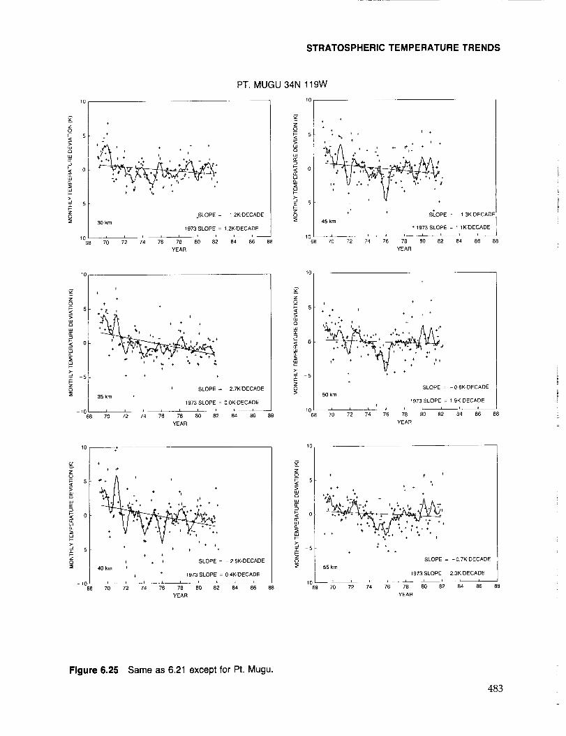
STRATOSPHERIC TEMPERATURE TRENDS
o_z
>
o
i 5
0
1068
PT. MUGU 34N 119W
+
+
+ J_ * + + +÷ + +
+ + ,% +* ÷ **_ + *
÷_i ÷ ++ . +4-+++÷ + + +
+ _ +
÷SLOPE = 1 2K.DECADE
30 km
1973 SLOPE = 1.2K DECADE
i / i • i _ L L I --70 72 74 76 78 80 82 84 86 88
YEAR
Q +
5 +*_+ ;+ + +++ + + + ÷+ + ÷ + _. # +
+ , ++
# + + ¢ + ++ + 4_. * + +
+ + ++ +
+ + SLOPE _ 1 3K DECADE45 km
I + 1973 SLOPE 1 1K DECADE/
68 70 72 74 76 78 80 82 84 86 88
YEAR
10
5
3>
D
o,,=,0,.
++
+
+ +
.+t+ • ÷
• _ + + .
+++ _+ +_+ !+++ + +. + + +,++
+ _ + + % -_+
+ SLOPE = -2.7K'_DECADE
35 km
1973 SLOPE = 0.0K..DECADE
- 106B 70 72 74 6 78 80 8
YEAR
g-
5
a
l--
>_,5
zO5
+ • *
+ + ++ ÷ +
• + +
• +
• * / 2
÷
SLOPE - 0 6KDECADE
50 km
1973 SLOPE = 1 9K DECADE+
68 70 72 74 78 80 82 8 8
YEAR
10
£3
I 58
+
+ ++
+ + + +,+t+ + ++ +_ ++ •
++ +
+ + ÷
+ +
+ + ÷ SLOPE = - 2.5K,DECADE
40 km +++ 1973 SLOPE = 0.4K.'DECADE
10 i / [ .... • t i 1 i _. _68 70 72 74 76 78 80 82 94 86 88
YEAR
10
Z
o5
t-,
(3£
>,I 5
O
÷ t ÷
÷ + ÷ _+ ÷
V_" t+'+ + ",'*k,,_-+;/_+/ + t + +/_h,_
*;It_. t*+k;_.411 ,D++ +_+ *# ++ +
÷+ _ ÷ ++ + ÷
÷+ + ÷
+ + +
SLOPE = -0.7K DECADE
55 km
1973 SLOPE - 23K'DECADE
-_ 7_-;, ......1068 70 76 78 80 82 84 86 98
YEAR
Figure 6.25 Same as 6.21 except for Pt. Mugu.
483
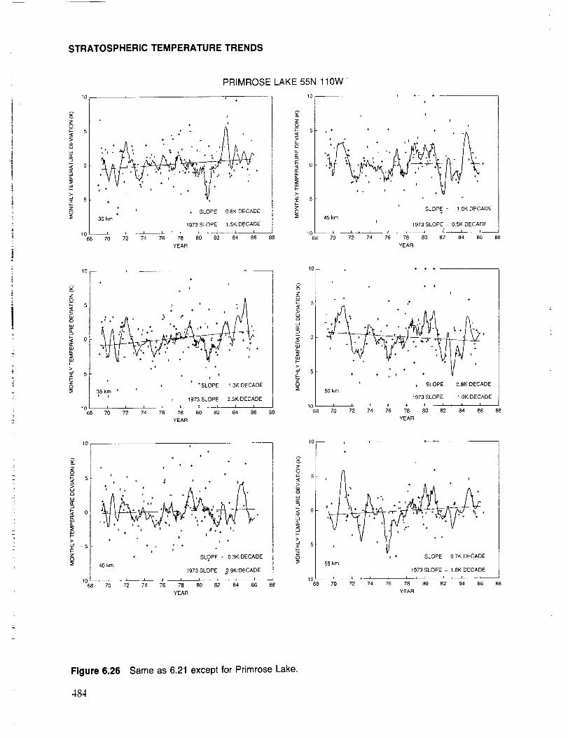
STRATOSPHERIC TEMPERATURE TRENDS
PRIMROSE LAKE 55N 110W
10 + 10 --
_Zz_o
i0rr
5§
L
YEAR
++
+ +
+ * +. + ÷ +
A ^+#.+ + %
i +
++ + SLOPE 0.SK DECADE+
30 km
1973 SLOPE 1.5K DECADE
z_o_ 6
o
o_
_ 6g
+
++÷
÷
+ ÷ + ÷ , ÷ +
+ + + +
+ ÷ t +++ +
+ + + ++ + ,
+ , ÷ + ÷÷ ÷ ÷
_ ÷ •
+ +
+SLOPE = 1 OK DECADE
45 km+
1973 SLOPE 05K DECADE
t0 _ _ _ /_ _
68 70 72 74 76 78 80 82 84 86 88
YEAR
10 --
F-
5
O
1068
+ ...... +
÷+
÷+
+ ÷ +
+ ÷ ÷ ÷ +
+ + +++ ++
++ + ÷_
* ÷
÷ ÷
+ _. t ++ +
÷+ + +
+ ÷+
÷ +÷ + SLOPE 13K DECADE
35 km + +
+ t973 SLOPE 2,5K DECADE
70 7 76 7 80 82 84 86 88
YEAR
10
5__. 5>
<_ o
,,=,I.->-
5F-ZO
÷
÷++
+
÷ ++
÷ + _ ÷ + +
+ ÷÷+ ÷ + + _++ + + _+
÷÷ ÷
+ + ++
÷ + + + +
, ÷ ÷ 4-+ + +
+ SLOPE = 03KDECADE
40 km
1973 SLOPE ,09K.'DECADE
__ _ i i_ _ i I0 i i i1068 70 72 74 76 78 82 84 86 88
YEAR
10-- _ ÷ 4- 4-
Z
o.>,E3
0
==f-
5
1068
++ + +
÷
+ +÷ ++
+ +
+ + ** +
+ + + + + ++ + +%
+ +
+ +÷
+ ÷
+ SLOPE 0 8K DECADE*50 km
1973 SLOPE 1 0K'DECADE
74 76 78 80 82 84 86 88
YEAR
10--
_Z
< 5
0
o._
T 5
O
1068
+ ÷ _- .
4,
+
÷
÷
÷ ÷+ _,
÷ ÷4-÷ ÷ ## + _ ÷ +*
+ ÷, _'÷÷
÷ " SLOPE 07K DECADE
55 km
1973 SLOPE = 1 8K DECADE
' ;_........ _--;_870 74 76 78 80 82 8
YEAR
Figure 6.26 Same as 6.21 except for Primrose Lake.
484

STRATOSPHERIC TEMPERATURE TRENDS
6.4 MECHANISMS FOR ATMOSPHERIC TEMPERATURE TRENDS
In this section, the processes that could drive stratospheric temperature changes are dis-
cussed. Over the last 10 years during which satellite measurements have been available, the solar
flux, the level of aerosol loading, and the concentrations of trace gases all have changed.
Dynamical processes may also contribute to temperature changes. This section outlines the
changes in temperature expected from these effects. If most of the processes contributing to the
observed stratospheric temperature trends of the last decade can be quantitatively assessed,
then it may be possible to infer the reliability of reported ozone changes (e.g., SBUV, SAGE,etc.), as well as model-computed ozone changes.
6.4.1 Global Ozone Changes
In this section, calculations that estimate temperature changes that would result from the
global changes in ozone reported by the SBUV and SAGE data processing teams aresummarized.
SBUV ozone-mixing ratios have been reported to be declining since 1979, with a maximum
decrease of 20 percent at I mb from 1979 to 1986. Radiative equilibrium temperature calculations
were made using 1979 and 1986 zonal mean SBUV ozone-mixing ratio profiles, at 80°N in Juneand 0 ° in March. These two cases were chosen because they represent situations in which
dynamical effects should be minimal (Geller et al., 1983). Thus radiative equilibrium temperature
computations may provide a reasonable assessment of temperature trends. Figure 6.27 showsSBUV ozone fractional decreases between 1979 and 1986.
The calculations are performed using three different radiative transfer models, as shown in
Table 6.11. In Models 1 and 2, the tropospheric water vapor profiles are taken from the
McClatchey (McClatchey et al., 1971) tropical and subarctic reference atmospheres for the
equatorial and the polar calculations, respectively. Stratospheric water vapor is fixed at 5 ppmv,
and the ground temperature is set equal to the air surface temperature. Model 3 has a simplified
troposphere and specifies infrared fluxes and tropospheric albedos based on mean values that
give approximately the correct upwelling flux at 100 rob. For the tropical equinox calculation, thesolar declination angle is fixed at 0°, while for the summer polar calculation, the declination is
fixed at 23.5. The surface albedo is set to 0.7 for the polar case and 0.07 for the tropical case, and
no clouds are included. The temperatures are time-marched to radiative equilibrium using
diurnally averaged solar heating.
Figure 6.28 shows the radiative equilibrium temperature changes resulting from the 1979 to
I986 SBUV ozone changes for the June polar case; Figure 6.29 shows the changes for the March
equatorial case. The models are in remarkably close agreement. A maximum temperature
decrease of 6.7-7.2K at about 0.5 mb occurs for the June polar case, while a decrease of 5.2-5.5K
at 0.5 mb occurs for the March equatorial case. For both cases, the region of maximum cooling is
fairly narrow, falling to zero by 2 rob. A temperature difference this sharply peaked may be
difficult for satellites having broad instrument weighting functions (see Figure 6.2) to detect.When these temperature changes are convolved with the synthesized SSU-47X weighting
function centered at 0.5 mb, the temperature changes that are predicted to be observed by
satellite are reduced to - 4.8K for the June polar and - 3.8K for the March equatorial cases. The
2-year averaged SSU-47X differences (i.e., the 1985 through 1986 data differenced with the 1979
through 1980 data) shown in Table 6.10 show a global change of - 1.75K, while SSU-36X (shownin Table 6.9) shows a global change of - 1.4K.
485
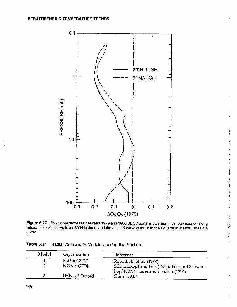
STRATOSPHERIC TEMPERATURE TRENDS
..Q
Ev
ILln"
O009LUn"Q_
0.1
m
m
m
q
10-
100-0.3
I t
I/
//
III
\\\\
\
X\
\\ \ I
I, I", 1\1
\
/ I/
/
///
/ ''t/ \_/ t
-o.1 0
A03/03 (1979)
I I
IIII80°N JUNE
0o MARCH
[I1
M
m
m
m
m
I
0.1 0.2
Figure 6.27 Fractional decrease between 1979 and 1986 SBUV zonal mean monthly mean ozone mixingratios. The solid curve is for 80°N in June, and the dashed curve is for 0° at the Equator in March. Units areppmv.
Table 6,11 Radiative Transfer Models Used in this Section
K
i5.
|
=
h
L
Model Organization
1 NASA/GSFC
2 NOAA/GFDL
3 Univ. of Oxford
Reference
Rosenfield et al. (1988)
Schwarzkopf and Fels (1985), Fels and Schwarz-
kopf (1975), Lacis and Hansen (1974)
Shine (1987)
486

STRATOSPHERIC TEMPERATURE TRENDS
0.1
10
100-8
i I i I _ i =¸ 1 1 I 1,1/I I i I i
/ ,,_,-" MODEL 2
MODEL 3 -" -: _"_
i.
JUNE POLAR /
TEMPERATURE :,,_
DIFFERENCES_z_ __L_J_ _,_'_
-7 6 -5 -4 -3 -2 -1
DEGREES(K)
t I i
0 1 2
Figure 6.28 Radiative equilibrium temperature differences computed by the three models for the June
summer polar case. The differences plotted are computed using 1986 and 1979 ozone data,
Figure 6.29
Ev
LUn"
03O3LUEEQ_
0.1
1 -
10
100-8
l I l I l I : I t I :/I l I t
MODEL1 J /
MODEL 3 _""J
/ o ooeL
MARCH EQUATORIALTEMPERATURE _./z_
DIFFERENCES /#1I I I I I I __._.z__l___. i , I
-7 -6 -5 -4 -3 -2 -1 0 1
DEGREES(K)
As in Figure 6.28 except for the March equatorial case.
i I i
2
487

STRATOSPHERIC TEMPERATURE TRENDS
The radiative temperature changes expected on the basis of the changes in ozone measured
by the SAGE-I and SAGE-II instruments, which give an independent estimate for the periodbetween 1980 and 1986 (cf. Chapter 5), are considered below. The SAGE data used are zonal
mean profiles for a latitude band 15°S to 15°N and represent annual averages constructed from
seven periods, during which both SAGE-I and SAGE-II sampled the Equator within roughly the
same 30-day period of the year. It is important to realize that SAGE measures ozone only
between 26 and 50 km. Because the predicted temperature is sensitive to the ozone change above50 km, two cases have been considered: no ozone change outside 26 to 50 km, and - 5 percent
ozone change above 50 km and -2 percent below 26 km.
Figure 6.30 shows the ozone profiles, and the solar heating and radiatively induced
temperature changes computed from Model 2 for the two cases. Notice that, at 47 km, both casespredict changes of about 1K, but above 50 km, the two cases disagree. It remains true, however,
that both scenarios yield temperature changes much smaller than those predicted using theSBUV ozone discussed above.
When convolved with the appropriate SSU weighting functions 47X and 36X, the satellite-
measured temperature changes are calculated to be:
SSU Channels SAGE SAGE SBUV
Case (a) Case (b)47X - 0.4 - 1.2 - 3.6
36X -0.2 -0.3 -1.8
Wrv
¢/}W
rvQ_
.01
.03
0.1
0.3
1.0
3.0
10.0
30.0
1000
q I
SAGE 1986-1980
"1
k)
!t
CASE1
CASE2
l
looo.o [ ..... I I 1 I I I20 10 0 10 -2 1 0 2 -1
03/03(%) 3Jsw (DEGREE,DAY) 3T(K)
.I
>,
8O
- 64
48 >r---I
c
rn
332
16
02
Figure 6.30 Radiative equilibrium computation for SAGE-observed ozone.
488

STRATOSPHERIC TEMPERATURE TRENDS
6.4.2 The Radiative Impact of Other Trace Gases
Significant changes are occurring in the middle atmosphere concentration of other radiatively
active gases such as CO2, CH4, and N20. In the upper stratosphere, a near radiative balanceexists between solar radiation absorbed by ozone and infrared radiation emitted by carbon
dioxide, ozone, water vapor, and other trace gases. Higher levels of stratospheric trace gases
increase infrared emittance and will produce a decrease in temperature. Fels (private communi-
cation, 1987) has computed that the increased cooling caused by CO2 alone to yield a -0.2 to
- 0.3K change in temperature at 2 mb and a - 0.15K change at 10 mb between 1979 and 1986. It is
not likely that the expected changes in trace gases other than ozone could significantly modify
the upper stratosphere temperature.
6.4.3 Solar Cycle
The solar UV flux that affects the 30 to 70 km region lies between wavelengths of 200 and 300
nm, where the Hartley absorption bands of ozone are located (see WMO, 1986). The radiation
absorbed by ozone at these wavelengths gives rise to a strong heating, with a peak at 50 km.
During the course of the solar cycle from its maximum to its minimum, the incident UV flux at
the top of the atmosphere decreases. This implies a decrease in the stratospheric heating rates,
provided the ozone amounts remain unchanged (an assumption made throughout this section).The change in the UV flux (200 to 300 nm) is not uniform. While the flux at 205 nm changes by
about 9 percent, that at 270 nm changes by about I percent. A one-dimensional radiative transfermodel (Ramaswamy and Kiehl, 1985) is used to investigate the effects of the change in the
Hartley band flux at the top of the atmosphere upon the heating rates during solar maximum and
solar minimum. The wavelength-dependent reduction applied is based on the results of Heath
and Schlesinger (1986) (see also Chapter 7). The resulting changes in the tropical stratospheric
heating rates (Figure 6.31) are expressed as the difference between the values at the time of
9O
7O
v
5o(.9LLI"r
3O
10
CHANGE IN SOLAR HEATING OVER
A SOLAR CYCLE
L I I
I t I
-0.1 0.2 -0.3
AJ(K'd)
-0.4
Figure 6.31 Changes in solar heating rates due to variations in the ultraviolet flux between solar minimumand solar maximum based on Heath and Schlesinger (1986) and Chapter 7 of this report. Units are degrees
Kelvin per day.
489

STRATOSPHERIC TEMPERATURE TRENDS
E
v
I-"1-(.9
LLI"1-
9O
7O
5O
30
10
CHANGE IN R-C ETEMPERATURE OVER
A SOLAR CYCLE
I
I
0 -1 -2
&T(K)
Figure 6.32 Changes in radiative-convective equilibrium temperature due to changes in the solar ultra-violet flux over a solar cycle.
solar minimum and those during the solar maximum. The maximum change, about 0.15K per
day, occurs where the absolute values are peaked (50 kin).
These heating perturbations are treated as a driving force in a radiative-convective equi-
librium model (Fels et al., 1980) to investigate the resulting changes in the temperature structure(ozone amount is held fixed). As shown by the results in Figure 6.32, the profile of the
temperature perturbations is similar to the profile of the heating rate perturbations. The change
in the temperature between the solar minimum and the solar maximum at 50 km in the presentcalculation is about 0.8K.
6.4.4 Aerosols
Stratospheric aerosol loadings caused by volcanic emissions possess the potential to alter thetransfer of radiation and perturb the energy balance of both the troposphere and the strato-
sphere. Radiative-convective model studies (Pollack et al., 1976; Hansen et al., 1978) have
shown that the principal radiative effects of volcanic aerosols (composed typically of ash and
sulfuric acid) are to reduce the solar flux in the troposphere and to cause a warming in the lower
stratosphere. Part of this warming is a result of aerosol absorption in the solar spectrum, while
the other part is caused by absorption of the longwave flux from the troposphere and the
subsequent reemission at the colder stratospheric temperatures. As an example of the possible
magnitude of this warming, Pollack and Ackerman (1983) estimate an increase in temperature of
about 3.5K at 30 mb in the northern tropics due to the E1 Chich6n volcanic cloud.
The magnitude of the warming in the lower stratosphere that results from volcanic emissions
depends on the aerosol optical properties, their sizes, and the upwelling longwave flux from the
490

STRATOSPHERIC TEMPERATURE TRENDS
troposphere, all of which exhibit considerable spatial and temporal variations. The nature of
these dependencies is illustrated here for a diurnally averaged tropical atmospheric profile,
using a one-dimensional radiative transfer and a radiative-convective model (Ramaswamy andKiehl, 1985). For the purposes of the present sensitivity study, the aerosols are assumed to have a
lognormal size distribution, with a constant number concentration between 16 and 25 km; it may
be noted that this was a typical altitude for the E1 Chich6n debris. The optical depth at a
wavelength of 0.5 microns is assumed to be 0.08, unless stated otherwise.
The effects of the optical property and the size of the particulates are examined by considering
three different cases: 1) a unimodal size distribution (mode radius of 0.08 micron) composed of
spherical sulfate drops (optical properties from Palmer and Williams, 1975), 2) a bimodaldistribution (two mode radii, 0.02 and 0.2 micron) containing larger particles, characteristic of
the El Chich6n debris at some locations, and 3) unimodai distribution of dust particles with the
same size characteristics as in (1), but with different optical properties (Shettle and Fenn, 1979).
The difference between (1) and (2) is due to the size distribution, while the difference between (1)
and (3) is due to the optical properties.
The initial perturbations in the solar heating rates for each of the three cases are shown in
Figure 6.33a; the perturbations in the longwave heating are shown in Figure 6.33b. Since
sulfates absorb only in the near infrared, while dust absorption extends over the entire solar
spectrum, the dust-induced solar heating exceeds that caused by the sulfates for similarly sized
particles; the sulfates, however, are stronger absorbers than dust in the longwave spectrum.
Larger sulfate particles result in increased longwave heating rates. The temperature per-
turbations are shown in Figure 6.33c. The vertical profile of the changes in the temperature is,
CHANGES IN HEATING RATES AND TEMPERATURE
DUE TO STRATOSPHERIC AEROSOLS
25 , I/ t I /i I 1 I I l I _l
(a) / // " r \
// ./ "ill�I� IF/ ,<,"
,, llsS.]i/ IllS!
1o _ i i i l IIiiI i I l
-0.1 0 0.1 0.2 0.3 0.4 0.5 0 0.1 0 2 4 6 8
A QSOL (K/d) A QLW (K"d) _T(K)
UNIMODAL (SMALL SIZE) SULFATE AEROSOL
BIMODAL (SMALL & LARGE SIZE) SULFATE AEROSOL
UNIMODAL (SMALL SIZE) DUST AEROSOL
Figure 6.33 Effect of aerosols with an optical depth of 0.08 on a) the solar heating rate, b) the infraredheating rate, and c) the temperature, for a tropical profile. The solid curve is unimodal sulfate, the dashedcurve bimodal sulfate, and the dot-dashed curve unimodal dust aerosol.
491
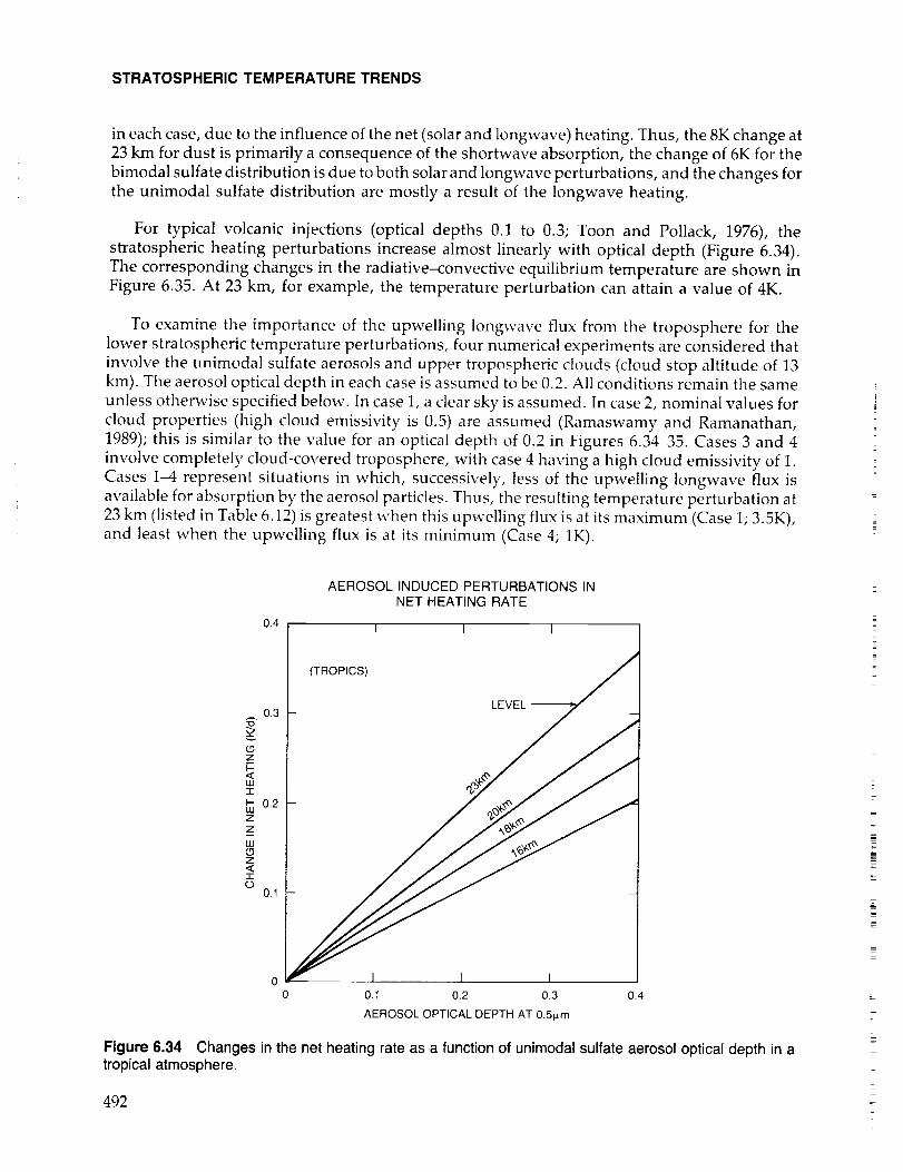
STRATOSPHERIC TEMPERATURE TRENDS
in each case, due to the influence of the net (solar and Iongwave) heating. Thus, the 8K change at
23 km for dust is primarily a consequence of the shortwave absorption, the change of 6K for the
bimodal sulfate distribution is due to both solar and longwave perturbations, and the changes forthe unimodal sulfate distribution are mostly a result of the longwave heating.
For typical volcanic injections (optical depths 0.1 to 0.3; Toon and Pollack, 1976), the
stratospheric heating perturbations increase almost linearly with optical depth (Figure 6.34).The corresponding changes in the radiative-convective equilibrium temperature are shown inFigure 6.35. At 23 km, for example, the temperature perturbation can attain a value of 4K.
To examine the importance of the upwelling longwave flux from the troposphere for the
lower stratospheric temperature perturbations, four numerical experiments are considered that
involve the unimodal sulfate aerosols and upper tropospheric clouds (cloud stop altitude of 13km). The aerosol optical depth in each case is assumed to be 0.2. All conditions remain the same
unless otherwise specified below. In case 1, a clear sky is assumed. In case 2, nominal values for
cloud properties (high cloud emissivity is 0.5) are assumed (Ramaswamy and Ramanathan,1989); this is similar to the value for an optical depth of 0.2 in Figures 6.34-35. Cases 3 and 4
involve completely cloud-covered troposphere, with case 4 having a high cloud emissivity of 1.
Cases 1-4 represent situations in which, successively, less of the upwelling longwave flux is
available for absorption by the aerosol particles. Thus, the resulting temperature perturbation at
23 km (listed in Table 6.12) is greatest when this upwelling flux is at its maximum (Case 1; 3.5K),and least when the upwelling flux is at its minimum (Case 4; 1K).
0.4
AEROSOL INDUCED PERTURBATIONS INNET HEATING RATE
I I I
(TROPICS)
L9Z
t--<LLI
'l-
F-LU
Z
Z
LU
(.9Z<"I-
(..)
0.3
0.2
0.1
LEVE
0
0 0.1 0.2 0.3 0.4
AEROSOL OPTICAL DEPTH AT 0.5_m
Figure 6.34 Changes in the net heating rate as a function of unimodal sulfate aerosol optical depth in atropical atmosphere.
492
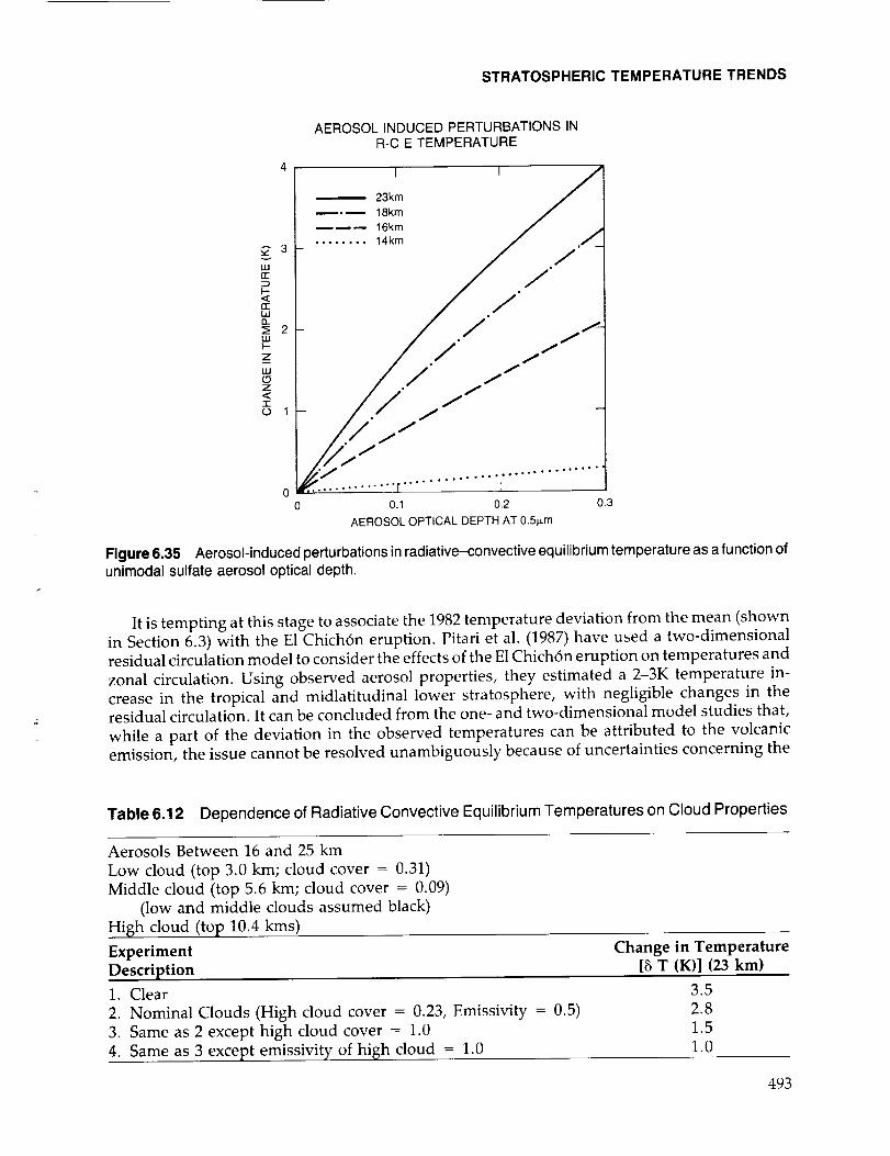
STRATOSPHERIC TEMPERATURE TRENDS
_" 3
UJ
rr
rrW
_ 2WI'--
Z
W
Z
T
AEROSOLINDUCED PERTURBATIONSINR-C E TEMPERATURE
23km
18km
16km
........ 14kin
/J
.. o,. °_°o''° ° =.°.°°°°
........ r ......... l0.1 0.2 0.3
AEROSOL OPTICAL DEPTH AT 0.5_m
Figure 6.35 Aerosol-induced perturbations in radiative-convective equilibrium temperature as a function ofunimodal sulfate aerosol optical depth.
It is tempting at this stage to associate the 1982 temperature deviation from the mean (shownin Section 6.3) with the E1 Chich6n eruption. Pitari et al. (1987) have used a two-dimensionalresidual circulation model to consider the effects of the E1Chichgn eruption on temperatures and
zonal circulation. Using observed aerosol properties, they estimated a 2-3K temperature in-
crease in the tropical and midlatitudinal lower stratosphere, with negligible changes in theresidual circulation. It can be concluded from the one- and two-dimensional model studies that,
while a part of the deviation in the observed temperatures can be attributed to the volcanicemission, the issue cannot be resolved unambiguously because of uncertainties concerning the
Table 6.12 Dependence of Radiative Convective Equilibrium Temperatures on Cloud Properties
Aerosols Between 16 and 25 km
Low cloud (top 3.0 km; cloud cover -- 0.31)
Middle cloud (top 5.6 km; cloud cover = 0.09)
(low and middle clouds assumed black)
High cloud (top 10.4 kms)
Experiment
Description
Change in Temperature[& T (K)] (23 km)
1. Clear
2. Nominal Clouds (High cloud cover = 0.23, Emissivity = 0.5)
3. Same as 2 except high cloud cover = 1.0
4. Same as 3 except emissivity of high cloud = 1.0
3.5
2.8
1.5
1.0
493
STRATOSPHERIC TEMPERATURE TRENDS
spatial and temporal variations in the aerosol optical properties. The problem of radiatively
active species interacting simultaneously with the microphysical and large-scale dynamical
processes must be addressed comprehensively before a definitive answer can be obtained from
the models. Further, observations of both aerosol properties and temperatures also need to be
accurate, since the lower stratosphere has a large radiative time constant.
6.4.5 Dynamics
The global circulation of the stratosphere is established largely through the interplay betweenthe external tropospheric forcing and the radiative heating and cooling within the stratosphere.
It has long been realized that trends in both temperature and ozone can result, in principle, from
dynamical trends in the stratosphere. These changes can result from an alteration in the level of
wave activity through tropospheric forcing or through changes in the wave propagation
characteristics of the stratosphere itself. The latter changes can result from changes in winds and
temperatures through a variation in the concentration of radiatively active gases, aerosols, or the
solar flux. Since the concentrations of the radiatively active gases are, in turn, influenced by the
transport properties of the stratosphere, which are partially determined by dynamical forcing, allof these processes are interdependent.
Eddy activity in the stratosphere tends to force the stratosphere away from a state of
near-radiative equilibrium. In the absence of dynamical activity, long-wave cooling would
balance short-wave heating everywhere except for small departures caused by thermal inertia
and the seasonal cycle. Therefore, trends in both stratospheric temperatures and trace gases
cannot be considered independent processes.
A number of authors have considered the feedbacks that might result from ozone depletions
or solar cycle changes altering the insolation, the large-scale winter jet structure, and ultimately
the propagation properties of large-scale waves (Schoeberl and Strobel, 1978; Fels et al., 1980;Callis et al., 1985b; Kiehl and Boville, 1988). These studies, which fixed the troposphere, found
no significant change in the stratospheric dynamical activity except for scenarios of very sizable
(>50 percent) ozone depletions. For example, using perpetual conditions from January, Kiehland Boville (1988) concluded that the dynamical response to halving ozone uniformly was small.
The dynamical response to a realistic ozone reduction scenario, with the largest ozone changes
confined to high latitudes, was found to be not only quite different to that for uniform ozonereductions, but even smaller.
An estimate of the tropical stratopause temperature change caused by altered dynamics may
be obtained by assuming that the globally averaged stratosphere at any level is in radiative
equilibrium. If it is assumed that the largest temperature changes are likely to be in the polar
night, and that these are, at most, on the order of 30K (Hamilton, 1982), then compensating
changes on the order of several degrees in the tropics would be expected. This estimate isconfirmed by Hamilton's analysis, which shows that even in years whose polar stratopause
temperatures differ by 30K, the tropical temperatures at 1 mb are the same to within a few
degrees. Thus, any dynamical process in the tropics cannot realistically be expected to mask the
long-term temperature changes that would result from the SBUV-reported ozone changes in the
upper stratosphere.
It is more difficult to assess how changes in the tropospheric forcing of the stratosphere might
alter the lower stratospheric temperature structure. Current three-dimensional model simu-
lations have difficulty even reproducing the observed stratosphere (Mahlman and Umscheid,
494
STRATOSPHERIC TEMPERATURE TRENDS
1984), although substantial improvements have been made by increasing the model resolution
(Mahlman and Umscheid, 1987). A possible reason for a change in the tropospheric forcing is a
change in the locations and intensity of convective regions. These regions can change in
response to alterations in the fluxes of sensible and latent heat that result from a change in
surface properties. While large-scale modification of the land surface has the potential to
produce significant changes in the surface fluxes, a more likely candidate is a change in thedistributions of sea surface temperatures and sea ice (e.g., Austin, private communication,
1987).
The sea surface temperature distribution is not independent of the atmospheric circulation.
The major ocean current systems are primarily wind driven, so that the sea surface temperature
distribution is intimately coupled with the atmospheric circulation on time scales ranging
upwards from about a month. This coupling of atmosphere and ocean has the potential tointroduce oscillations with time scales of years to millennia, which makes the definition and
identification of truly external forcing processes difficult. An example of a fluctuation of the
coupled ocean-atmosphere system is the E1 Niflo-Southern Oscillation (ENSO), which hasreceived a great deal of attention in recent years. Changes in the surface temperatures of the
tropical Pacific Ocean have been shown to introduce changes in tropical convection and in
planetary wave patterns in the extratropics of the Northern Hemisphere (see, e.g., Blackmon etal., 1983). There appears to be little doubt that variations in the tropical Pacific surface tempera-
tures are a manifestation of the coupling with the atmosphere, and even though a considerable
amount of work has been done on modeling the tropospheric response to sea surface tempera-tures, little information is available on the stratospheric response.
Figure 6.6 shows the long-term fluctuations in temperatures in the 30 to 100 mb layer at north
temperature latitude. The amplitude of these fluctuations was less than 1K over decadal periods;since the source of these changes has not been identified radiatively, it can be hypothesized that
they are dynamical in origin. Thus, a crude estimate of the magnitude of dynamical contributionsto trends could be 1K per decade in the lower stratosphere.
Long-term changes in tropospheric dynamical activity could certainly produce midlatitude
and polar stratospheric temperature trends as large as the observed year-to-year changes, andperhaps larger. These changes are as large as the predicted changes because of trends in the
radiative source gases discussed earlier; therefore, they will add to the uncertainty in identifyingtrend mechanisms from temperature observations alone. However, tropical stratospheric re-
sponses to midlatitude dynamical changes are expected to be quite small, so that unambiguoustrend detection may be possible in that region.
6.4.6 Radiative Photochemical Models
Radiative photochemical models predict a variation in stratospheric ozone and temperatureduring solar cycles and as the concentrations of ozone-catalyzing minor constituents increase
with time (see Chapter 7). The calculation of the expected change in stratospheric temperature is
complicated by feedbacks involving ozone photochemistry. For example, a decrease in tempera-ture leads to some increase in ozone, which acts to offset the original temperature decline.
Table 6.13 summarizes the results from one-dimensional models at the altitude of peak
cooling. All models listed are photochemical and include the effects of increased CO2, CH4, N20,and chlorofluorocarbons (and sometimes NOx). The resultant decreases in ozone are also
incorporated. The calculations are grouped into sets covering approximately the same period,
and the trend in degrees Kelvin per decade is given for comparison. Since the periods shown are
495

STRATOSPHERIC TEMPERATURE TRENDS
Table 6.13 Comparison of Calculated Cooling From One-Dimensional Radiative-Photo-chemical Models Near to the Level of Peak Cooling
Approximate Temp Approximate
Paper Period Level of Peak Change Change in temp/
Coolin8 decade
Brasseur and De Rudder 1960-80 45 km -3.4K -1.7K/decade
Bruhl 1960-85 1.5 mb (45 kin) -3.9K -1.6K/decade
Vupputuri 1960-85 (at 42 km) - 3.8K - 1.5K/decadeWuebbles 1960-83 42 km - 3.4K - 1.5K/decade
Brasseur and De Rudder 1940-80 45 km -5.0K -1.25K/decade
Bruhl 1935-85 1.5 mb (45 km) -4.9K -1.0K/decadeOwens et al. 1940-85 46 km -3.8K -0.84K/decade
Vupputuri 1940-85 (at 42 km) -4.5K - 1.0K/decade
Wang et al. 1950-80 48 km -1.9K -0.6K/decadeWuebbles 1950-80 42 km - 3.2K - 1.1K/decade
Bruhl 1860-1985 1.5 mb (45 km) - 6.0K - 0.48K/decade
Vupputuri 1850-1980 44 km - 5.5K - 0.42K/decade
roughly the length of an integral number of solar cycles, models that incorporate solar cycle
changes can be compared with those that do not. Most of the model-computed temperaturechanges in Table 6.13 are caused by changes in the ozone. Bruhl (1987), for example, calculates a
peak cooling of 1K between 1960 and 1985 for the CO2 only, and the CO2, CH4, and N20 only
scenarios; this compares with a value of nearly 4K when the chlorofluorocarbons are included.
The agreement between different model calculations is good, particularly for the cooling over
the past two or three decades. In the 40 to 50 km layer, these models predict a change of - 1.5 to- 1.7K over the last decade. The two-dimensional model computations presented in Chapter 7
give similar results.
Table 6.14 shows the cooling calculated at around 30 mb (24 km) for the same sets of
calculations. The agreement between calculations is not as good as might be expected near a
transition level. Bruhl's model, in particular, calculates a smaller cooling at 30 mb, since the
height at which tropospheric warming changes to stratospheric cooling is several kilometersabove the transition level found in other models. This level is particularly difficult to calculate
and will depend on the particular convective scheme incorporated in the troposphere, as well ason other modeling details, such as vertical resolution. Thus trends estimated at the 30 mb level
are likely to be subject to a greater uncertainty than those at lower pressures.
6.5 CONCLUSIONS
The stratospheric satellite, rocket, and radiosonde data sets analyzed in this chapter have
been intercompared in detail. Temperature changes from 1979 to 1986 have been determined
using radiosondes (Free University of Berlin and Angell and Korshover 1983a) and satelliteradiances (United Kingdom Meteorological Office and NMC data). Radiosonde data above 30mb were not considered reliable for trend determination. The rocket data used here have been
edited extensively and improved so that the results are not comparable to previous studies. Therocket data and zonal mean satellite data were intercompared, and trends were determined over
the longer rocket data period.
496

STRATOSPHERIC TEMPERATURE TRENDS
Table 6.14 Comparison of Calculated Cooling From One-Dimensional Radiative-Photo-chemical Models at About 30 mb (24 km)
Paper Period
Approximate Temp Approximate
Level of Peak Change Change in temp/
Cooling decade
Bruhl 1960-85 30_mb (24 km) almost zeroLabitzke et al. 1970-80 24 km -0.2K -0.2K/decade
Labitzke et al. 1960-85 24 km -0.6K -0.24K/decade
Vupputuri 1960-85 25 km - 0.8K - 0.32K/decadeWuebbles 1960-83 24 km - 0.45K - 0.2K/decade
Owens et al. 1940-85 24 km - 0.6K - 0.13K/decade
Vupputuri 1940-85 25 km - 1.2K - 0.27K/decade
Wang et al. 1950-80 24 km -0.2K -0.07K/decadeWuebbles 1950-83 24 km - 0.47K - 0.14K/decade
Bruhl 1860-1985 30 mb (24 km) -0.3K -0.02K/decade
Vupputuri 1850-1980 25 km - 1.6K - 0.12K/decade
This chapter also includes an investigation of the processes that could produce stratospheric
temperature trends. These processes include global changes in ozone, solar flux, concentration
of other trace constituents, and aerosol loading, as well as dynamical changes. The majorconclusions are outlined below:
• The radiosonde and satellite data sets generally intercompare very well, although some
periods of disagreement exist. Figure 6.17 shows the computed difference in global
temperatures for 1985/86-1979/80. The largest global decline is in the upper stratosphere,
with a computed change of -1.75K + 1.0K.
• The rocket data have insufficient spatial coverage to establish global trends and are subject
to some uncertainties. Longer term trends from rocketsondes starting in 1969 indicate a
cooling on the order of - 1 to - 2K per decade in the mid- to upper stratosphere. However,
if the trends are calculated starting in 1973, they range from - 1K per decade up to 2K per
decade (warming). Hence, rocketsonde trends are subject to large uncertainties.
• Long-term trends in the lower stratosphere derived from radiosonde-based data sets show
no significant cooling except in the Tropics and over Antarctica.
• There is a warming of the lower and middle stratosphere in the 1982-1983 period, which
appears to be associated with, and is consistent with, radiative heating of the E1 Chich6naerosol cloud.
• Standard interactive photochemical and radiative transfer models estimate a cooling of theupper stratosphere of - 1.2 to - 1.7K per decade for 1970-1990 because of the ozone and
trace gas changes. Since 1979, an additional cooling of -0.8K has occurred due to a
decrease in the solar flux as part of the solar cycle.
497

STRATOSPHERIC TEMPERATURE TRENDS
• Using the reported SBUV ozone changes from 1979 to 1986, a radiative equilibrium tropical
temperature decline of 5.5K can be computed. An additional 0.8K decline is expected as aresult of the decrease in solar flux over that phase of the solar cycle. When this change is
convolved with the SSU 47X weighting function centered at 0.5 mb, the detectable tempera-
ture change is -4.6K. This compares to the observed - 1.3K _+1K tropical change (Figure
6.18). Thus, the reported SBUV ozone changes in the upper stratosphere appear to be
inconsistent with the observed temperature changes, while SAGE-reported ozone changesare not.
498

![Stratospheric temperature trends from GPS-RO and Aqua AMSU ... · COSMIC-10, Estes Park, Sep. 25, 2017. Main findings in Khaykin et al. [GRL, 2017] Temperature trends over 14 years](https://img.dokumen.tips/doc/110x75/5f815a141b018d4ef135d336/stratospheric-temperature-trends-from-gps-ro-and-aqua-amsu-cosmic-10-estes.jpg)


