Stratospheric variability and trends in IPCC model … · Stratospheric variability and trends in ... Stratospheric variability and trends ... 20 Observational climatologies of temperature

Stratospheric variability and trends in IPCC model

simulations

E. C. Cordero, P. M. De F. Forster

To cite this version:

E. C. Cordero, P. M. De F. Forster. Stratospheric variability and trends in IPCC modelsimulations. Atmospheric Chemistry and Physics Discussions, European Geosciences Union,2006, 6 (4), pp.7657-7695. <hal-00302056>

HAL Id: hal-00302056

https://hal.archives-ouvertes.fr/hal-00302056

Submitted on 9 Aug 2006

HAL is a multi-disciplinary open accessarchive for the deposit and dissemination of sci-entific research documents, whether they are pub-lished or not. The documents may come fromteaching and research institutions in France orabroad, or from public or private research centers.

L’archive ouverte pluridisciplinaire HAL, estdestinee au depot et a la diffusion de documentsscientifiques de niveau recherche, publies ou non,emanant des etablissements d’enseignement et derecherche francais ou etrangers, des laboratoirespublics ou prives.

https://hal.archives-ouvertes.fr

https://hal.archives-ouvertes.fr/hal-00302056

ACPD6, 7657–7695, 2006

Stratosphericvariability and trends

E. C. Cordero andP. M. de F. Forster

Title Page

Abstract Introduction

Conclusions References

Tables Figures

J I

J I

Back Close

Full Screen / Esc

Printer-friendly Version

Interactive Discussion

EGU

Atmos. Chem. Phys. Discuss., 6, 7657–7695, 2006www.atmos-chem-phys-discuss.net/6/7657/2006/© Author(s) 2006. This work is licensedunder a Creative Commons License.

AtmosphericChemistry

and PhysicsDiscussions

Stratospheric variability and trends inIPCC model simulationsE. C. Cordero1 and P. M. de F. Forster2

1Department of Meteorology, San Jose State University, San Jose, CA 95192, USA2School of Earth and Environment, University of Leeds, Leeds, LS2 9JT, UK

Received: 24 July 2006 – Accepted: 6 August 2006 – Published: 9 August 2006

Correspondence to: E. C. Cordero ([email protected])

7657

http://www.atmos-chem-phys-discuss.net

http://www.atmos-chem-phys-discuss.net/6/7657/2006/acpd-6-7657-2006-print.pdf

http://www.atmos-chem-phys-discuss.net/6/7657/2006/acpd-6-7657-2006-discussion.html

http://www.copernicus.org/EGU/EGU.html

ACPD6, 7657–7695, 2006



Title Page



Tables Figures

J I

J I

Back Close

Full Screen / Esc



EGU

Abstract

Atmosphere and Ocean General Circulation Model (AOGCM) experiments for the In-tergovernmental Panel on Climate Change Fourth Assessment Report are analyzedusing both 20th and 21st century model output to better understand model variabil-ity and assess the importance of various forcing mechanisms on stratospheric trends.5

While models represent the climatology of the stratosphere reasonably well in compar-ison with NCEP reanalysis, there are biases and large variability among models. Ingeneral, AOGCMs are cooler than NCEP throughout the stratosphere, with the largestdifferences in the tropics. Around half the AOGCMs have a top level beneath ∼2 hPaand show a significant cold bias in their upper levels (∼10 hPa) compared to NCEP,10

suggesting that these models may have compromised simulations near 10 hPa due toa low model top or insufficient stratospheric levels. In the lower stratosphere (50 hPa),the temperature variability associated with large volcanic eruptions is either absent (inabout half of the models) or the warming is overestimated in the models that do includevolcanic aerosols. There is general agreement on the vertical structure of temperature15

trends over the last few decades, differences between models are explained by the in-clusion of different forcing mechanisms, such as stratospheric ozone depletion and vol-canic aerosols. However, even when human and natural forcing agents are included inthe simulations, significant differences remain between observations and model trends,particularly in the upper tropical troposphere (200 hPa–100 hPa), where, since 1979,20

models show a warming trend and the observations a cooling trend.

1 Introduction

General Circulation Models (GCMs) are important tools for assessing how natural andanthropogenic forcings affect our climate and their predictions form the basis of ourknowledge of future climate change. Climate models have evolved and improved into25

the currently used coupled Atmosphere Ocean GCMs (AOGCMs). To better represent

7658





ACPD6, 7657–7695, 2006



Title Page



Tables Figures

J I

J I

Back Close

Full Screen / Esc



EGU

the many physical processes, horizontal and vertical resolution has also increased.Current models whose data will be used in Intergovernmental Panel on Climate Change(IPCC) fourth assessment report (AR4) focus on simulating the response of the sur-face and troposphere. The stratosphere of most of these models tends to be poorlyresolved. In contrast, past stratospheric ozone assessment reports (e.g., WMO, 2003)5

tend to use data from models that focus resolution on the stratosphere. For a num-ber of reasons it is becoming increasingly apparent that accurate simulations of thestratosphere are important to determine the evolution of the surface climate and otheraspects of climate change.

1) Stratospheric temperature trends may provide some of the best evidence for at-10

tributing climate change to humans (Ramaswamy et al., 2006; Santer et al., 2005;Shine et al., 2003; Tett et al., 1996). Different climate forcing mechanisms such ascarbon dioxide and solar constant changes are more readily distinguishable in theirstratospheric response, compared to their surface response, which is often very sim-ilar between forcing agents (e.g., Forster et al., 2000). Further, human and natural15

effects can also be readily distinguished in tropopause height changes, which are aproduct of the tropospheric warming and stratospheric cooling associated with manyhuman forcing agents (Santer et al., 2003a, b).

2) It has been shown that stratospheric variability and changes, particularly in theNorthern and Southern Hemisphere polar vortices can affect the weather and climate20

of the troposphere (e.g., Shindell and Schmidt, 2004; Thompson et al., 2005). Inparticular Thompson et al. (2005) and Gillett and Thompson (2003) showed that partof the surface cooling in and around Antarctica could be associated with stratosphericozone loss affecting the stratospheric polar vortex. In addition, several papers (e.g.,Miller et al., 2006; Stenchikov et al., 2002) show that strong tropical volcanic eruptions25

(e.g., Mt. Pinatubo) and ozone depletion can both affect the winter arctic oscillation inthe Northern Hemisphere. However it also appears that a well resolved stratosphere isrequired to accurately produce the correct tropospheric response (Gillett et al., 2002;Sigmond et al., 2004)

7659





ACPD6, 7657–7695, 2006



Title Page



Tables Figures

J I

J I

Back Close

Full Screen / Esc



EGU

3) Several forcing or feedback mechanisms have a component associated with thestratosphere. Modeling the effects of stratospheric ozone depletion and explosive vol-canic eruptions have benefited from a better representation of the stratosphere (2001).Solar irradiance changes may also have an effect on surface climate through inducingdynamical changes in the stratosphere (Haigh, 2001; Haigh et al., 2005; Rind, 2002,5

2004). It is also important to resolve stratospheric water vapor changes as these canhave a large effect on surface climate, as well as in the stratosphere (e.g., Forster andShine, 2002). For example Stuber et al. (2001) found that the ECHAM4 GCM hada very strong feedback associated with stratospheric water vapor increases resultingfrom tropopause temperature increases.10

Pawson et al. (2000) designed an intercomparison to compare and characterize thestratosphere using GCMs from a variety of modeling groups. In this paper we repeataspects of this intercomparison for the current IPCC AOGCMs which were not specif-ically designed for stratospheric simulation. To aid climate-change attribution, we thenexpand this intercomparison to look at temperature trends in the stratosphere simu-15

lated since 1958, and compare these to observations.The primary goal of this paper is to evaluate the ability of the participating IPCC

models to simulate the structure, variability and trends of the lower stratosphere dur-ing the 20th century. Understanding the strengths and weaknesses not only providesfeedback to the modeling community, but can also communicate to the larger public20

the uncertainties of predictions for the 21st century. In Sect. 2, a brief descriptionof the IPCC models and various observation-based datasets are given. Model sim-ulations and their comparisons with observations are given in Sect. 3, while Sect. 4is devoted to understanding the temperature trends in the stratosphere over the lastthree decades. Section 5 describes 21st century temperature trends, and Sect. 6 is25

a discussion regarding the vertical profile of temperature trends. We finish with ourconclusions in Sect. 7.

7660





ACPD6, 7657–7695, 2006



Title Page



Tables Figures

J I

J I

Back Close

Full Screen / Esc



EGU

2 Model and observed data

The analysis uses AOGCM simulations from the IPCC Model archive at the Programfor Climate Model Diagnosis and Intercomparison (PCMDI). Nineteen AOGCM simula-tions submitted to the archive from groups in ten different countries are compared usingwind and temperature fields from the climate of the 20th century experiments. These5

models incorporate various natural and anthropogenic forcings including changes inozone distribution, greenhouse gases and aerosols distribution, although not all mod-els incorporate all of these forcing mechanisms. A list of the model forcings directlyrelevant to the stratosphere is given in Table 1 and will be discussed further in the nextsection.10

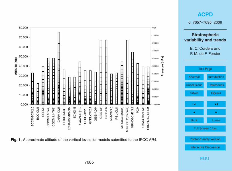
The submitted model simulations record data at 17 vertical levels in the atmosphere(1000, 925, 850, 700, 600, 500, 400, 300, 250, 200, 150, 100, 70, 50, 30, 20, 10 hPa).The actual model top and number and placement of stratospheric levels vary frommodel to model, and are shown in Fig. 1. While the majority of models do have amodel top above 10 hPa, the number of levels above the tropopause and the vertical15

resolution varies widely. Of the 19 models, only eight have more than three levels above10 hPa. This scarcity of model levels in the stratosphere may be a significant impair-ment to accurately resolving the large scale structure and variability of the stratosphere(Hamilton et al., 1999).

Observational climatologies of temperature are used from both satellite and ra-20

diosonde observations. These include data from the Microwave Sounding Unit (MSU)carried on the NOAA polar orbiting satellites. Retrievals from the MSU provide at-mospheric temperature at broadly defined levels of the troposphere and lower strato-sphere. In this study, we use a climatology of MSU temperature data compiled byRemote Sensing Systems (RSS, Mears et al., 2003, of channel 2 (MSU2) and channel25

4 (MSU4) retrievals of monthly and zonally averaged gridded temperature anomaliesbetween 1979–1999.

We use two radiosonde datasets compiled from the groups at the Hadley Centre

7661





ACPD6, 7657–7695, 2006



Title Page



Tables Figures

J I

J I

Back Close

Full Screen / Esc



EGU

(HadAT2; Thorne et al., 2005) and the NOAA (RATPAC-A; Free et al., 2005). Thesedatasets, which use subsets of the global radiosonde network and span the years1958–2004, are compiled into monthly average temperature anomalies. While theserecently developed radiosonde climatologies incorporate various adjustments to ac-count for data inhomogeneities (Free et al., 2004), a recent analysis by Randel and Wu5

(2006) suggests a systematic cold bias in the RATPAC-A tropical lower stratosphericdata compared to the MSU satellite observations. This potential cold bias in the trop-ical lower stratosphere radiosonde observations will be considered in the subsequentmodel comparisons. A further description of the uncertainties regarding the MSU andradiosonde observations is given in the discussion of Sect. 6.10

The model data will also be compared to the National Center for Environmental Pre-diction /National Center for Atmospheric Research (hereafter NCEP) Reanalysis. TheNCEP data are derived using atmospheric general circulation models in a data as-similation system using in-situ and remotely sensed observations (Kistler et al., 2001).The NCEP reanalysis is available from 1948, but for stratospheric comparisons, only15

since the beginning of satellite observations in 1979 are the data likely to be reliablefor global stratospheric studies (Randel et al., 2004). Although the ERA-40 reanalysisdataset has a higher range of altitudes, there are not significant differences betweenNCEP and ERA-40 for the global and zonally averaged fields examined in this study,and thus we will restrict the presentation of our results to the NCEP reanalysis.20

3 20th century climate: model intercomparison

The AOGCMs participating in the IPCC model comparison represent the most ad-vanced and comprehensive set of climate simulations so far produced. Simulations forthe 20th century have been compared with each other and with available observations.In Table 1, we identify a subset of forcings used in the IPCC simulations of the 20th cen-25

tury climate that directly influence the stratosphere. The information on model forcingwas largely obtained from the IPCC model website, where modeling groups supplied

7662





ACPD6, 7657–7695, 2006



Title Page



Tables Figures

J I

J I

Back Close

Full Screen / Esc



EGU

information about their runs. For model simulations where the supplied information didnot appear to match the model temperature simulations, a note was made. While allthe models include the steady increase in greenhouse gas forcing, the models differin their inclusion of variations in stratospheric ozone depletion, volcanic aerosols andvariations in solar radiation. In the following section, an analysis of model experiments5

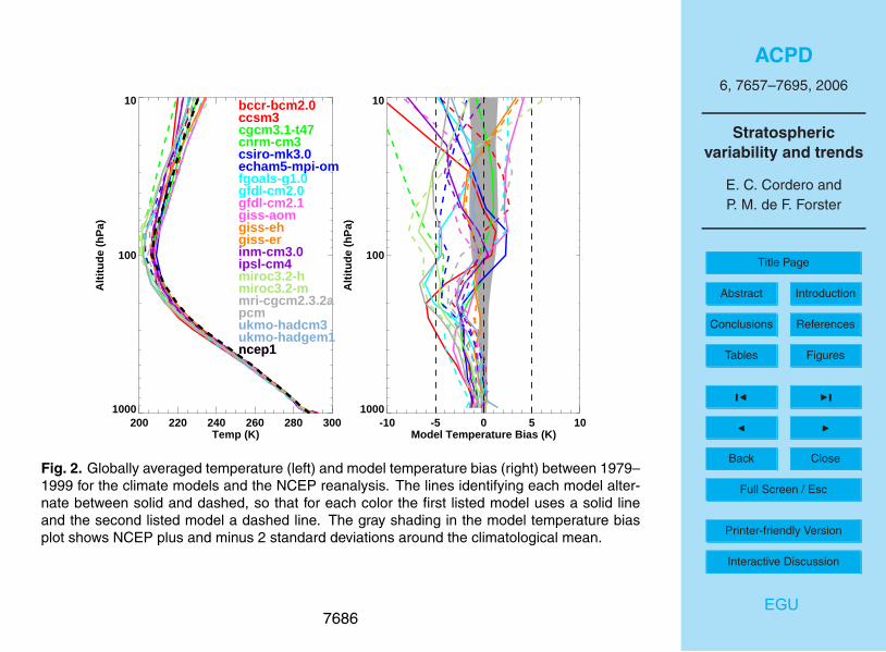
is made to assess model performance and the role of various forcing processes.Figure 2 shows a vertical profile of the annual average global temperature from the

IPCC models and the model temperature bias with respect to the NCEP reanalysis.The temperature distribution is averaged between 1979–1999 and ranges from thesurface to 10 hPa. The temperature distribution illustrates the delineation in lapse rate10

between the troposphere and stratosphere, and the minimum in temperature at thetropopause. Near the surface and throughout the middle troposphere, the IPCC mod-els agree reasonably well with each other and are generally within 2–3 K of the NCEPreanalysis, while at higher altitudes, the spread among the models increases. For ex-ample, at 700 hPa, the range of IPCC models differ by only ∼3 K, while at 200 hPa and15

10 hPa, the models differ by 6 K and 17 K, respectively. Although the standard deviationin the NCEP reanalysis shows that the natural variability in global mean temperature islarger in the troposphere compared to the stratosphere, models have larger differencescompared to each other and larger biases compared to NCEP in the stratosphere com-pared to the troposphere. In addition, the models generally underestimate the global20

temperature in the stratosphere, a common GCM characteristic observed in variousmodel intercomparisons (e.g., Austin et al., 2003; Pawson et al., 2000). AOGCM tem-peratures throughout most of the upper to the middle troposphere are also cooler thanNCEP, a result we will explore further in Sect. 4.

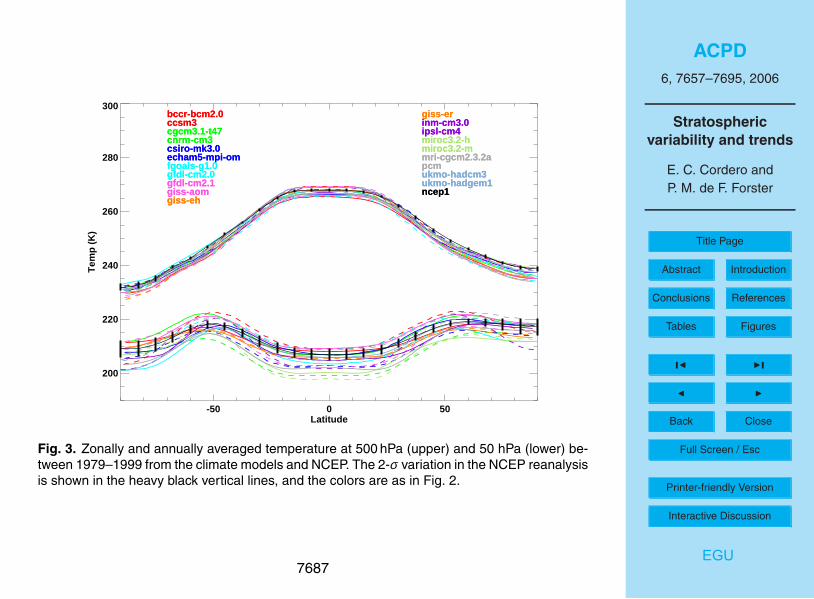
A comparison of zonally averaged temperatures averaged between 1979–1999 at25

500 hPa and 50 hPa from the models and NCEP is displayed in Fig. 3. In the middletroposphere, the models are within 5 K of each other and the NCEP reanalysis, withthe uncertainty in NCEP less than 5 K at all latitudes. At 500 hPa the largest differencebetween models and observations is seen at the polar NH, where the models are

7663





ACPD6, 7657–7695, 2006



Title Page



Tables Figures

J I

J I

Back Close

Full Screen / Esc



EGU

consistently colder than NCEP. An evaluation of seasonal temperature variations (notshown) shows that during both December, January, February (DJF) and June, July,August (JJA), most models are cooler than NCEP in the NH, while in the SH, theredoes not appear a similar bias. In the stratosphere, the range of temperatures betweenmodels is larger than in the troposphere, with a spread in magnitude of about 11 K5

in the tropics and poles and a slightly smaller range at midlatitudes. As shown bythe uncertainty in the NCEP reanalyses, the natural variability in the stratosphere andespecially near the polar stratosphere is larger than in the troposphere.

At the poles, the models generally are in reasonable agreement with the NCEP anal-yses, with no apparent cold pole biases that was a feature of older versions of GCMs10

(e.g., Pawson et al., 2000). In fact, the corresponding winter (DJF) polar temperaturesin the NH are almost all within the NCEP uncertainty, while in the SH, of the 11 mod-els that are outside the NCEP uncertainty, eight of the model are biased warm. Inthe tropics, a majority of the model simulations are cooler than the reanalysis, and themodel to model variability is larger than in the extratropics, while the natural variability15

in the tropics is actually smaller than in the poles. Thus, the cooling bias seen in theglobal average temperature (Fig. 2), at least at 50 hPa, is not from a cold pole bias,but rather more by biases in the tropical latitudes. The tendency changes at higheraltitudes, where a cold pole bias is seen in many models. During DJF, 14/19 of themodels are colder than the observed variability between 70–90◦ N, while during JJA,20

14/19 are colder than the observed variability between 70–90◦ S. These results implythat model representation of the planetary wave spectrum in the lower stratosphere ofthe winter hemisphere may be reasonable, while higher up this may not be the case.A natural question is then what role does the location of the model lid and number ofstratospheric levels have on these results?25

To evaluate the potential role of the vertical resolution and location of the model lidon the structure of stratospheric temperature, we group the models into two categoriesbased on the altitude of the model lid and then examine the seasonal temperaturevariation between models and NCEP at three latitude ranges (70–90◦ N, 30◦ N–30◦ S

7664





ACPD6, 7657–7695, 2006



Title Page



Tables Figures

J I

J I

Back Close

Full Screen / Esc



EGU

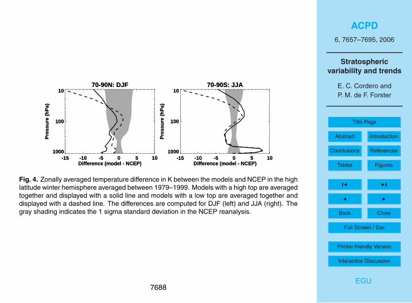
and 70–90◦ S) during the winter of each hemisphere (Fig. 4). The first group is labeled“high” and has a model lid at or above 45 km (∼2 hPa; indicated as high in Table 1)while the second group is labeled “low” has a model lid below 45 km. Figure 4 illus-trates the results of this comparison showing the difference (model – NCEP) for thetwo model groups in the high latitude winter hemisphere. During DJF and JJA, the dif-5

ference between models with low and high tops is only significant near 10 hPa, the topreporting altitude for the IPCC dataset. In both cases, the models with a lower top (andfewer stratospheric levels) have a cold bias at 10 hPa of nearly 15 K, while the highertop models have a corresponding cold bias of between 4–7 K. There does not seemto be any statistically significant bias at lower altitudes. For example, at 50 hPa, the10

differences in biases for the two model groups are around 2 K during both seasons andwithin the variability of the NCEP reanalyses. These results suggest that the locationof the model top, or related to this the number of stratospheric levels, affects modelstructure near 10 hPa in the winter hemisphere.

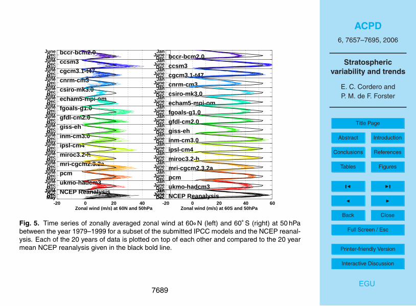
The evolution of stratospheric winds is related to temperature variations and ulti-15

mately controlled by large scale wave activity. In Fig. 5, the annual cycle in zonal windat 60◦ N and 60◦ S at 50 hPa is displayed for each of the IPCC models and the NCEPreanalysis for the years 1979–1999. In the NH, the winds are westerly and strongestduring winter (DJF) and easterly and weak in the summer (JJA). By plotting each yearon the same scale, the interannual variability can also be estimated. While overall there20

is reasonable agreement with NCEP in terms of the timing of the maximum westerlywinds, there exist significant variations in the peak magnitude of the westerly windsand the magnitude of the interannual variability. The interannual variability in NH DJFwinds range from ∼6 m s−1 in the CSIRO model to almost 20 m s−1 in the MRI model,compared to NCEP which is also around ∼20 m s−1.25

The variability in the SH is markedly different compared with the NH. The year toyear variability of peak westerly winds ranges from 4–10 m s−1, almost half the vari-ability seen in the NH. The smaller variability in the SH polar winds indicates a weakerplanetary wave spectrum and is generally consistent with observation (Newman and

7665





ACPD6, 7657–7695, 2006



Title Page



Tables Figures

J I

J I

Back Close

Full Screen / Esc



EGU

Nash, 2005). While the maximum winds reach over 50 m s−1 in a couple of the mod-els, the NCEP reanalysis maximum winds appears larger than all the models exceptthe CCSM3 model. However, because few reliable radiosonde observations in themiddle to high latitude southern hemisphere exist, biases may exist at these locations(Randel et al., 2004). At higher altitudes, the magnitude of the winter winds increases5

in both hemispheres, as does the range of variability between models.A comparison between zonal winds at 60◦ N and 60◦ S (Fig. 5) suggests that while

hemispheric variations between the poles are reasonably captured, important depar-tures from the observed climatology exist. This suggests that variations in dynamicsand the characterization of large scale waves in IPCC models may inhibit the ability of10

models to accurately resolve stratospheric variability and change.

4 20th century trends

The primary radiative forcing mechanisms responsible for global temperature changesin the stratosphere over the last three decades have been increases in well-mixed GHGconcentrations, declines in stratospheric ozone, explosive volcanic eruptions and so-15

lar changes (e.g., Ramaswamy et al., 2006). Increases in stratospheric water vapormay also influence global temperature trends (e.g., Shine et al., 2003). As the futurepromises further changes in all of these forcing processes, temperatures in the strato-sphere will continue to change.

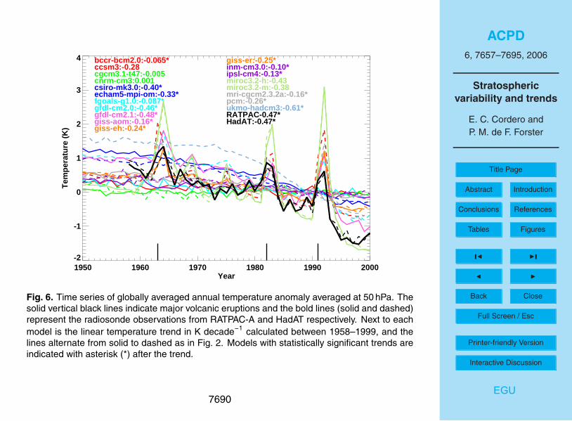
Figure 6 shows the global temperature anomaly at 50 hPa from the IPCC models20

between the years 1950 and 1999. The temperature anomaly is computed with respectto the average temperature computed between 1985–1995. The model time series areidentified by colored lines and the model trends, calculated between the years 1958–1999, are given in K decade−1 next to the model name. Trends are determined froma linear regression, while a Student t-test is performed to determine if the trend is25

statistically significant. In cases where the trend is statistically significant at the 95%levels, an asterisk (*) is placed next to the trend. The heavy black solid and dashed

7666





ACPD6, 7657–7695, 2006



Title Page



Tables Figures

J I

J I

Back Close

Full Screen / Esc



EGU

lines indicate the RATPAC-A and HadAT2 radiosonde observations respectively.Model temperatures at 50 hPa show that the majority of models indicate some cool-

ing since 1958, with generally larger cooling rates since 1980. The cooling trend rangesfrom −0.06 to −0.61 K decade−1 in models with statistically significant trends, com-pared to the radiosonde observations that both show a statistically significant cooling5

of ∼0.47 K decade−1. Among the models examined, 14 out of 19 (12 out of 19) showa statistically significant cooling trend between 1958–1999 (1979–1999). However,among these models, the majority underestimate the observed radiosonde trend, withonly four models (CSIRO-mk3.0; gfdl-cm2.0/2.1; ukmo-hadcm3) near or above the ra-diosonde trend. The two simulations by miroc3.2h/m were also close to the observed10

trend, but were not statistically significant probably due to high variability caused byexcessive sensitivity to volcanoes.

The most apparent feature in the 50 hPa temperature time series outside of the cool-ing trend are the three warming perturbations corresponding to the volcanic eruptionsof Mt. Agung (1963), El Chichon (1982) and Mt. Pinatubo (1991). The warming results15

from increases in the absorption of incoming solar radiation and the absorption of out-going infrared radiation by volcanic aerosols (Ramaswamy et al., 2001). As indicatedin the forcing table (Table 1), nine of the models used for the IPCC include volcanicperturbations, although it was reported that two other models also included volcanicperturbations and yet did not show any corresponding temperature response. The20

model warming associated with the Mt. Agung eruption in 1963 ranges from 0.5 K to2.0 K compared to the radiosonde observations which warmed globally by about 0.8 Kover a year. In the later eruptions, a similar magnitude of model temperature responseis found, with the Mt. Pinatubo eruption providing the largest temperature response asseen by radiosonde observations and satellite observations (Free and Angell, 2002;25

Karl et al., 2006). Radiosonde observations after Mt. Pinatubo show a warming ofabout 1 K, while the models that include volcanic aerosols generally overestimate thistemperature response: for the models including volcanic aerosols, the temperatureincrease from 1990 to 1992 ranges from 1.0 to 2.5 K.

7667





ACPD6, 7657–7695, 2006



Title Page



Tables Figures

J I

J I

Back Close

Full Screen / Esc



EGU

At higher altitudes (10 hPa; not shown), cooling trends are consistently larger and themagnitude of temperature variations associated with volcanic perturbations is reduced.Qualitatively, the trend toward stronger cooling with altitude generally agrees with theresults of Shine et al. (2003) at 10 hPa and will be discussed further below.

Global model trends at altitudes from the surface to 10 hPa calculated between5

1958–1999 are compared with the corresponding radiosonde observations in Fig. 7.The 2-sigma uncertainty in the HadAT2 and RATPAC-A radiosonde trends are alsoshown. The radiosonde trends, which are in good overall agreement with each other,show warming within the troposphere between 0.1 to 0.2 K decade−1 at the surface tobetween 0.1 to 0.3 K decade−1 up to 250 hPa. Between 200 and 150 hPa, the crossover10

point between tropospheric warming and stratospheric cooling in both radiosonde ob-servations are collocated, while there are large differences among the models. Above100 hPa, atmospheric cooling increases with altitude up to about −0.5 K decade−1 at50 hPa. Model predictions generally range from 0.05 to 0.2 K decade−1 at the surfaceto 0.1 to 0.3 K decade−1 at 250 hPa. In the upper levels, the range of model trends be-15

comes wider, ranging from −0.6 to 0 K decade−1 at 50 hPa, compared to a radiosondecalculated trend of −0.5 K decade−1. While the majority of models are within the 2-sigma uncertainty of the radiosonde observations in the lower and middle troposphere(e.g., at 500 hPa, 16/19 models are within the uncertainty), in the upper troposphereand lower stratosphere, the majority of models show not enough cooling and are out-20

side the uncertainty (e.g., at 50 hPa, 4/19 models are within uncertainty). While acooling bias in the temperature trends derived from radiosonde observations may ex-ist (e.g., Randel and Wu, 2006; Seidel et al., 2004), most models simulate the paststratospheric temperature trends quite poorly.

A potential explanation for why some of the models used for the IPCC compare25

poorly to radiosonde temperature trends is the absence of stratospheric ozone deple-tion (Ramaswamy et al., 2006; Shine et al., 2003). As illustrated in Table 1, of the 19models that we compare for the 20th century, all models include well-mixed greenhousegas forcing while only 11 include stratospheric ozone depletion. To explore this further,

7668





ACPD6, 7657–7695, 2006



Title Page



Tables Figures

J I

J I

Back Close

Full Screen / Esc



EGU

temperature trends for models with and without ozone depletion are compared in Fig. 8for the two time periods of 1958–1999 and 1979–1999. The simulations are separatedbased on the inclusion of stratospheric ozone depletion and model temperature trendsare averaged in these two groups. The temperature trends from the RATPAC-A andHadAT2 radiosonde observations are also averaged, and the 2-sigma estimate of the5

trend uncertainty is indicated using horizontal lines. For the calculations of temperaturetrend between 1979–1999, satellite-derived trends computed from the RSS MSU anal-yses and their 2-sigma uncertainty are also shown, along with the approximate verticalrange of these observations.

In the trend calculations for both time periods, the models that include ozone de-10

pletion are significantly closer to the observations than the models that omit ozonevariations. In the trend between 1958–1999, the 50 hPa trend for the models withozone depletion average almost −0.4 K decade−1 while the models without ozone de-pletion are around −0.1 K decade−1. In this case, the models with ozone depletion arewithin the range of uncertainty for the radiosonde observations. In the lower strato-15

sphere/upper troposphere near (150–100 hPa), even models with ozone depletion falloutside the uncertainty of radiosonde observations, while below 150 hPa, the modelswith ozone depletion are within the radiosonde uncertainty and the models withoutozone depletion remain outside the observations all the way down to 700 hPa.

The crossover point between the tropospheric warming and stratospheric cooling20

is also significantly different between the two model groups. The models with ozonedepletion show a crossover point at around 150 hPa, while the models without ozonedepletion show a crossover point at 70 hPa or about 4.8 km higher in altitude. From200 hPa down to the surface, the models including ozone depletion are within the rangeof uncertainty for the radiosonde observations, while the models without ozone deple-25

tion are warmer than the observations down to 500 hPa.The global trends computed for the years 1979–1999 show a similar overall pattern

compared to the 1958–1999 data, although the rate of the tropospheric warming andstratospheric cooling is greater over the last two decades. The larger stratospheric

7669





ACPD6, 7657–7695, 2006



Title Page



Tables Figures

J I

J I

Back Close

Full Screen / Esc



EGU

cooling since 1979 is not surprising considering most ozone depletion has occurredsince 1979. In addition, the models also show better agreement to each other, andwith both radiosonde and satellite observations from the surface to 300 hPa. At higheraltitudes, however, the spread between the two model groups is larger than during1958–1999. At 50 hPa, the temperature trend is −0.6 K decade−1 for the models with5

ozone depletion and −0.1 K decade−1 for the models without ozone trends, while theradiosonde and satellite observations are −0.8 K decade−1 and −0.45 K decade−1 re-spectively. These results are qualitatively consistent with Shine et al. (2003) who foundsignificant divergence in the magnitude of model derived vertical temperature trendseven when the same ozone trend datasets were employed in different models. As10

discussed previously, it has been suggested that radiosonde trends in stratosphericcooling may be too large as a result of instrument biases at tropical latitudes (Randelet al., 2006). Indeed there is better agreement between the models and the satelliteobservations, although at 70 hPa, the models including ozone depletion are within theuncertainty of both observational datasets.15

Temperature trends in the tropics (30◦ N–30◦ S) calculated between 1979–1999 areshown in Fig. 9. From 50 hPa up to 10 hPa, the results look quite similar to the globalmodel trends. The models that include stratospheric ozone depletion produce a largercooling trend compared to models that do not. At these altitudes, the magnitude ofthe radiosonde trends is similar for the global and tropical averages, although the 2-20

sigma uncertainty in the tropical trend is about 20% larger than the global value. In thelower stratosphere and upper troposphere, the models show larger warming trends inthe tropics compared with the global trends. At 150 hPa, the tropical trends with andwithout ozone depletion are between 0.1 and 0.2 K decade−1 more positive than theglobal trends. The crossover point between tropospheric warming and stratospheric25

cooling for the models including stratospheric ozone depletion is around 150 hPa forthe global dataset and nearly 100 hPa for the tropical data. These changes are alsoreflected in the radiosonde observations, where the crossover point is estimated at250 hPa globally and near 200 hPa in the tropics. Thompson and Solomon (2005)

7670





ACPD6, 7657–7695, 2006



Title Page



Tables Figures

J I

J I

Back Close

Full Screen / Esc



EGU

found similar vertical profiles of temperature trends over 1979–2003 using both NCEPreanalysis and radiosonde datasets.

Below 200 hPa, the models and both satellite and radiosonde observations show sta-tistically similar magnitudes in tropical warming trends, although the models are sys-tematically warmer than the observations. The maximum warming trend in the tropical5

troposphere occurs near 300 hPa at around 0.3 K decade−1, while the maximum warm-ing trend in the global troposphere occurs near 200 hPa at around 0.2 K decade−1. Thelarger warming in the tropics compared to the extratropics has been observed in pre-vious model intercomparisons (e.g., IPCC, 2001) and the larger warming in the freetroposphere compared to the surface was also identified in some observational trends10

and in the current group of IPCC models (Karl et al., 2006; Santer et al., 2005). Thedifference between the average models with and without ozone depletion in the uppertroposphere and lower stratosphere (200 hPa–50 hPa) is less in the tropics comparedto the global trends.

This analysis illustrates the importance of including ozone variations for accurate15

calculations of trends in the lower stratosphere and upper troposphere. The significantdifference between the two groups of models suggests that inclusion of ozone trendsis critical to correctly modeling the long-term temperature variability in the stratosphereand may also be important to tropospheric climate. It is also noted that during the1979–1999 period, two large volcanic eruptions produced large temperature pertur-20

bations and thus increased the uncertainty of the trend calculation during this period.Thus, the inclusion of volcanic aerosol is also important for assessing long-term climatevariations in the stratosphere.

5 21st century climate predictions

Long term changes in radiative forcing over the next few decades will continue to impact25

global mean temperature in both the troposphere and stratosphere. Because many ofthe chemical reactions that affect ozone are sensitive to stratospheric temperature, it

7671





ACPD6, 7657–7695, 2006



Title Page



Tables Figures

J I

J I

Back Close

Full Screen / Esc



EGU

is important to establish an understanding of the range of possible future temperaturetrends to facilitate more realistic predictions of how ozone will change in the future.

The models used for the IPCC have been run with various emission scenarios forthe 21st century. In this study, we will focus on the A2 and B1 scenarios from theSpecial Report on Emissions Scenarios (SRES, IPCC, 2000) that differ primarily in the5

emissions of well-mixed green house gases. In the A2 scenario, concentrations of CO2increase from today’s value (∼380 ppmv) to approximately 850 ppmv by 2100, while theB1 scenario reaches 550 ppmv by 2100 (IPCC, 2001). These two scenarios reflect themost likely extremes for CO2 concentrations by the end of the century. The coupledmodels used for the 2001 IPCC report produce increases in global surface temperature10

of between 1.5 and 4.5 K by 2100 when forced with these scenarios.Figure 10 shows a time series of temperature anomaly between 2000–2100 at

50 hPa from the fifteen models that submitted 21st century simulations. In these sim-ulations, the future well-mixed GHG concentrations are specified by the A2 scenario,while ozone concentrations, which are not computed interactively, range from some15

type of ozone recovery to a constant value during the 21st century. While all modelsimulations show 50 hPa global temperatures declining over the 21st century, the rangeof predictions varies from −0.5 to −3.5 K by 2100. Differences in model ozone concen-trations over the 21st century are likely responsible for some of the range in modelpredictions.20

The relative uncertainty in model predictions of stratospheric temperature is furtherillustrated in Fig. 11, which shows the globally averaged temperature trend computedduring the 21st century for the IPCC models using the A2 and B1 scenarios. The trendsare calculated between 2010 and 2090 and thus reflect the range of possible temper-ature changes through the 21st century. In both the troposphere and stratosphere, the25

different emission scenarios produce significantly different trends. In the troposphere,the simulations using the A2 scenario show a surface warming near 0.3 K decade−1,and increasing up to 0.5 K decade−1 at 300 hPa. The weaker forcing in the models us-ing the B1 scenario produces a much smaller tropospheric response peaking at 0.25 K

7672





ACPD6, 7657–7695, 2006



Title Page



Tables Figures

J I

J I

Back Close

Full Screen / Esc



EGU

decade−1 at 300 hPa. The crossover altitude between warming and cooling is indepen-dent of emission scenarios and occurs near 70 hPa. This is a similar crossover altitudeas found in the 20th century simulations using the models that did not include ozonevariations and mirrors the signature of well-mixed GHG forcing. In the stratosphere, therate of cooling increases with increasing altitude up to around −0.7 K decade−1 for the5

A2 scenario and −0.4 K decade−1 for the B1 scenario. These simulations point to thechanging nature of both the stratosphere and troposphere and the large role emissionsplay in shaping their future temperature.

It should be emphasized that these models do not include interactive chemistry andthus cannot accurately predict the interaction between decreasing chlorine levels that10

affect ozone concentrations and increasing greenhouse gases that affect temperature.While declines in stratospheric ozone also act to cool the stratosphere, at some pointin the future global ozone levels will gradually begin to rise (WMO, 2003). In the strato-sphere, higher ozone levels will increase the amount of stratospheric ozone heatingwhich will at least partially offset the cooling due to increases in GHGs. Because15

ozone concentrations are sensitive to the background temperature field, understandingthe complex interaction between changing constituent concentrations and temperaturerequires an evaluation of the coupling between chemistry, radiation and atmosphericdynamics (Cordero and Nathan, 2005; Tian and Chipperfield, 2005). One exampleof this interaction is how the large cooling rates present in the upper stratosphere de-20

crease the temperature dependent ozone destruction and are forecast to produce asuper recovery in ozone where future total column ozone levels are actually higherthan pre-halogen levels (Eyring et al., 2006). It should be acknowledged that be-cause these interactions are not resolved in the IPCC AOGCMs, accurate predictionsof stratospheric temperature trends, especially those in the lower stratosphere, cannot25

be expected without reasonably accurate ozone predictions (Hare et al., 2004). In thepresent set of IPCC model simulations, the ozone forcing in the 21st century modelexperiments varies from constant ozone to a slow recovery by 2050.

Another challenge in accurately predicting stratospheric temperature in the 21st cen-

7673





ACPD6, 7657–7695, 2006



Title Page



Tables Figures

J I

J I

Back Close

Full Screen / Esc



EGU

tury concerns future changes in stratospheric water vapor. At present, there is not agood understanding of how stratospheric water vapor will evolve in the future, nor theprocesses governing these changes. For this problem, coupled climate chemistry sim-ulations that self consistently compute the interactions between radiatively active gasessuch as ozone and water vapor and large scale dynamics are again required (Austin et5

al., 2003).How well do the IPCC models compare with models that include interactive chem-

istry? In model experiments with doubled CO2 conditions including interactive ozonechemistry, substantial cooling is found throughout the middle atmosphere, with a maxi-mum cooling of ∼−3 K decade−1 near the stratopause and ∼−1.5 K decade−1 at 10 hPa10

(Jonsson et al., 2004; Sigmond et al., 2004). In recent coupled chemistry climate modelintercomparisons (Austin and Butchart, 2003; Eyring et al., 2006, 2005), the coolingtrend at 10 hPa is about −0.6 K decade−1 between 2000–2050. The weaker coolingtrend is in line with increasing ozone concentrations through the first half of the 21stcentury, but is also of similar magnitude as the trends from the models used for the15

IPCC. In a recent coupled chemistry-climate model (CCM) intercomparison (Eyring etal., 2006), an A1b scenario is used for the 21st century simulations, which is a middleforcing between the A2 and B1 forcings. In comparison to Fig. 11, the average trendcomputed by the CCM models is −0.6 K decade−1 at 10 hPa which falls within the A2and B1 IPCC model trends.20

Although there is some general agreement among models for how temperature willchange in the future, there remains significant uncertainty regarding how well dynam-ical processes are resolved in climate models. It is recognized that stratospherictemperature changes result from both direct radiative forcing (e.g., CO2, O3, volcanicaerosol and water vapor) and dynamical circulation changes induced by tropospheric25

changes, and that forcing mechanisms are linearly additive (Ramaswamy et al., 2006).However, our understanding of how these interactions may change in the future is stillpoor (Nathan and Cordero, 20061). In addition, various experiments using coupled cli-

1Nathan, T. R. and Cordero, E. C.: An ozone-modified refractive index for vertically propa-

7674





ACPD6, 7657–7695, 2006



Title Page



Tables Figures

J I

J I

Back Close

Full Screen / Esc



EGU

mate chemistry models found that the inclusion of interactive chemistry can alter modelmeteorology (Austin and Butchart, 2003; Manzini et al., 2003; Tian and Chipperfield,2005), coupling that was not included in the IPCC models. Finally, there remains signifi-cant uncertainty concerning dynamical processes associated with the parameterizationof gravity waves and propagation of planetary waves in global models (e.g., Austin et5

al., 2003; Shaw and Shepherd, 20062).

6 Discussion

Using MSU4 weighted temperature trends, Ramaswamy et al. (2006) recently at-tributed stratospheric temperature changes since 1979 to a combination of human andnatural factors. Good agreement between models and observations were found when10

including well-mixed greenhouse gas changes, ozone changes and natural solar andvolcanic changes. Each forcing contributed to the overall temperature-response timeseries. Their conclusions were based on results from a single model. Our findingsgenerally support their conclusion across a wide range of models. However, our resultsalso suggest that ozone and volcanic forcings need to be carefully evaluated and imple-15

mented in models. In particular, most models that included volcanic aerosols appearto have too much lower stratospheric (50 hPa) warming associated with Mt Pinatubo.

For many years there has been controversy over apparent differences in modeledand observed temperature trends in the free troposphere, comparing trends from ra-diosondes, satellites and models (e.g., NRC, 2004). The recent CCSP report (Karl et20

al., 2006) and the papers it cites (e.g., Fu et al., 2004) resolve many of these issues.Our findings also tend to support the conclusions of this report, that models and ob-served trends appear in agreement, within their respective uncertainties. However, theCCSP report also notes that in the tropics “while almost all model simulations show

gating planetary waves, J. Geophys. Res., submitted, 2006.2Shaw, A. T. and Shepherd, T. G.: Angular momentum conservation and gravity wave drag

parameterization: Implications for climate models, J. Atmos. Sci., submitted, 2006.

7675





ACPD6, 7657–7695, 2006



Title Page



Tables Figures

J I

J I

Back Close

Full Screen / Esc



EGU

greater warming aloft, most observations show greater warming at the surface”. Ourresults also support this conclusion. In particular they point to a real difference in theupper tropical troposphere. Since 1979 there seems to have been a real cooling trendin the radiosonde observations down to altitudes around 200 hPa, whereas in modelsit is almost impossible to get a cooling below 100 hPa. They all exhibit a typical moist-5

adiabatic type of response (see e.g., Karl et al., 2006). Although the cooling trendin radiosonde datasets could be up to 0.1 K decade−1 too large in this region (Randeland Wu, 2006) and radiosonde trends have many uncertainties, this difference appearsreal.

Reasons for this difference could be associated with convection schemes in the mod-10

els and/or their upper tropospheric water vapor feedback and/or resolution in the up-per troposphere. Much of the upper tropical troposphere (often termed the TropicalTropopause Transition layer or sub-stratosphere) is above typical altitudes of convec-tive outflow (e.g., Folkins et al., 1999; Gettelman and Forster, 2002; Thuburn and Craig,2000) and as such may behave more like part of the stratosphere (Forster et al., 1997;15

Thuburn and Craig, 2000). Forster and Collins (2004) also suggest that although thewater vapor feedback is generally well understood, the water vapor feedback in the up-per troposphere may not be particularly well represented by model simulations of theMt Pinatubo eruption. In the AOGCMs, relative humidity stays more or less constantwith altitude (Karl et al., 2006). If this is not occurring in reality or if stratospheric ra-20

diative processes are playing more of a dominant role in the 200–100 hPa region thanthe AOGCMs suggest, then temperature trends could be more negative than typicalmodels suggest in this region. Randel et al. (2006) suggest that recent temperaturechanges around the tropical tropopause could have been caused by a radiative re-sponse to a combination of ozone and water vapor changes; perhaps similar mecha-25

nisms are controlling the observed temperature trends in the 200 hPa–100 hPa regionand current AOGCMs are unable to capture these mechanisms. As the water vaporfeedback from this region is very important for tropospheric climate evolution, our worksuggests the need for a more focused effort to try and understand the large scale pro-

7676





ACPD6, 7657–7695, 2006



Title Page



Tables Figures

J I

J I

Back Close

Full Screen / Esc



EGU

cesses governing temperature trends in the region, as well as efforts to make sure thatAOGCMs can adequately simulate these responses.

7 Conclusions

AOGCM simulations submitted for the Fourth Assessment Report of the IPCC are an-alyzed to assess the ability of these models to simulate stratospheric variability and5

trends. Model temperature simulations between 1979–1999 are compared with NCEPreanalysis, and show that model to model variability is larger in the stratosphere com-pared to the troposphere, even when natural variability is considered. Model simula-tions that include volcanic aerosols are necessary to reproduce the observed interan-nual variability in the stratosphere, although most models that include volcanic aerosols10

tend to over predict the temperature response at 50 hPa. Although a cold temperaturebias in relation to NCEP is seen in a majority of the models throughout the stratosphere,the presence of a cold pole bias is only evident at 10 hPa during the winter. At 50 hPa,most models are within the NCEP variability in the NH winter, and within or warmerthan the NCEP variability in the SH winter. However, at 10 hPa, about half the models15

are between 10–15 K colder than NCEP. It appears that this difference is related torepresentation of the stratosphere within each model. In models with few stratosphericlevels and a relatively low model top, the cold pole bias is about 9 K larger than themodels with more stratospheric levels and a higher model top. This comparison sug-gests that in the present collection of models used by the IPCC, about half the models20

do not possess a high enough model top to accurately simulate stratospheric variabilityat 10 hPa. This shortcoming is expected to potentially affect other fields at 10 hPa andis likely to contribute to unrealistic variability at lower levels.

Stratospheric temperature trends in models are compared to existing radiosondeand satellite observed trends. In general, the models tend to underestimate the cool-25

ing trends in the stratosphere observed over the last forty years. The cooling of thestratosphere, which is largely controlled by declines in stratospheric ozone and in-

7677





ACPD6, 7657–7695, 2006



Title Page



Tables Figures

J I

J I

Back Close

Full Screen / Esc



EGU

creases in tropospheric GHGs, is only well simulated in models that include ozonedepletion over the last thirty years. However, in models that neglect ozone depletion,the temperature trends in the stratosphere do not show enough cooling. The largestdiscrepancy between model trends and observations is found in the upper troposphereand lower stratosphere, where even models that include ozone depletion do not cool5

as much as the observations. This discrepancy appears largest between 1979–1999,in tropical latitudes (30◦ N–30◦ S) between 100–200 hPa. Although tropical radiosondeobservations may themselves posses a spurious cooling trend, our analysis suggeststhat these differences appear real and should motivate further investigations to identifythe source of these differences.10

In the 21st century, model simulations using an A2 emission scenario all show thestratosphere continuing to cool, but with a wide range of projections. It is suggested,although not verified here, that differences in future ozone projections are responsiblefor a significant proportion of this range. Model simulations also show that the strengthof cooling in the stratosphere and warming in the troposphere are dependent on the15

emission scenario, but that the altitude of the crossover point between warming andcooling does not appear to change with emission scenario. These results illustratehow sensitive stratospheric temperature trends are to future well-mixed GHG concen-trations

Acknowledgements. We gratefully acknowledge the international modeling groups for providing20

their data for analysis, the Program for Climate Model Diagnosis and Intercomparison (PCMDI)for collecting and archiving the model data, the JSC/CLIVAR Working Group on Coupled Model-ing (WGCM) and their Coupled Model Intercomparison Project (CMIP) and Climate SimulationPanel for organizing the model data analysis activity, and the IPCC WG1 TSU for technicalsupport. The IPCC Data Archive at Lawrence Livermore National Laboratory is supported by25

the Office of Science, U.S. Department of Energy. E. C. Cordero is supported by NSF’s FacultyEarly Career Development Program (CAREER), Grant ATM-0449996 and NASA’s Living witha Star, Targeted Research and Technology Program, Grant LWS04-0025-0108. P. M. Forsteris supported by a Roberts Research Fellowship.

7678





ACPD6, 7657–7695, 2006



Title Page



Tables Figures

J I

J I

Back Close

Full Screen / Esc



EGU

References

Austin, J. and Butchart, N.: Coupled chemistry-climate model simulations for the period 1980to 2020: ozone depletion and the start of ozone recovery, Quart. J. R. Met. Soc., 129, 3225–3249; doi:10.1256/qj.02.203, 2003.

Austin, J., Shindell, D., Beagley, S. R., et al.: Uncertainties and assessments of chemistry-5

climate models of the stratosphere, Atmos. Chem. Phys., 3, 1–27, 2003.Cordero, E. C. and Nathan, T. R.: A New Pathway for Communicating the 11-Year Solar Cycle

Signal to the QBO, Geophys. Res. Lett., 32, L18805, doi:10.1029/2005GL023696, 2005.Eyring, V., Butchart, N., Waugh, D. W., et al.: Assessment of coupled chemistry-climate mod-

els:1. Evaluation of dynamics, transport characteristics and ozone, J. Geophys. Res., in10

press, 2006.Eyring, V., Harris, N. R. P., Rex, M., et al.: A strategy for process-oriented validation of coupled

chemistry-climate models, Bull. Am. Met. Soc., 86, 1117–1133, 2005.Folkins, I., Lowewenstein, M., Podolske, J. R., Oltmans, S. J., and Proffitt, M. H.: A barrier to

vertical mixing at 14 km in the tropics: Evidence from ozonesondes and aircraft measure-15

ments, J. Geophys Res., 104, 22 095–22 102, 1999.Forster, P. M. d. F., Blackburn, M., Glover, R., and Shine, K. P.: An examination of climate

sensitivity for idealised climate experiments in an intermediate general circulation model,Clim. Dyn., 16, 833–849, 2000.

Forster, P. M. d. F. and Collins, M.: Quantifying the water vapour feedback associated with20

post-Pinatubo global cooling, Clim. Dyn., 23, 207–214, 2004.Forster, P. M. d. F., Freckleton, R. S., and Shine, K. P.: On aspects of the concept of radiative

forcing, Clim. Dyn., 13, 547–560, 1997.Forster, P. M. d. F. and Shine, K. P.: Assessing the climate impact and its uncertainty for trends

in stratospheric water vapor, Geophys. Res. Lett., 29, doi:10.1029/2001GL013909, 2002.25

Free, M. and Angell, J. K.: Effect of volcanoes on the vertical temperature profile in radiosondedata, J. Geophys. Res., 107(D10), 4101, doi:1029/2001JD001128, 2002.

Free, M., Angell, J. K., Durre, I., et al.: Using first differences to reduce inhomogeneity inradiosonde temperature datasets, J. Clim., 17, 4171–4179, 2004.

Free, M., Seidel, D. J., Angel, J. K., et al.: Radiosonde atmospheric temperature products for30

assessing climate (RATPAC): a new dataset of large-area anomaly time series, J. Geophys.Res., 110, doi:10.1029/2005JD006169, 2005.

7679





ACPD6, 7657–7695, 2006



Title Page



Tables Figures

J I

J I

Back Close

Full Screen / Esc



EGU

Fu, Q., Johanson, C. M., Warren, S. G., and Seidel, D. J.: Contribution of stratospheric coolingto satellite-inferred tropospheric temperature trends, Nature, 429, 55–58, 2004.

Gettelman, A. and Forster, P. M. d. F.: Definition and climatology of the tropical tropopauselayer, J. Meteor. Soc. Japan, 80, 911–924, 2002.

Gillett, N. P., Allen, M. R., McDonald, R. E., et al.: How linear is the Arctic Oscillation response5

to greenhouse gases?, J. Geophys. Res., 107, doi:10.1029/2001JD000589, 2002.Gillett, N. P. and Thompson, D. W.: Simulation of recent southern hemisphere climate change,

Science, 302, 273–275, 2003.Haigh, J. D.: Climate variability and the influence of the sun, Science, 294, 2109–2111, 2001.Haigh, J. D., Blackburn, M., and Day, R.: The response of tropospheric circulation to perturba-10

tions in lower stratospheric temperature, J. Clim., 18, 3672–3691, 2005.Hamilton, K., Wilson, R. J., and Hemler, R. S.: Middle Atmosphere Simulated with High Vertical

and Horizontal Resolution Versions of a GCM: Improvements in the Cold Pole Bias andGeneration of a QBO-like Oscillation in the Tropics, J. Atmos. Sci., 56, 3829–3846, 1999.

Hare, S. H. E., Gray, L. J., Lahoz, W. A., O’Neill, A., and Steenman-Clark, L.: Can strato-15

spheric temperature trends be attributed to ozone depletion?, J. Geophys. Res., 109,doi:1029/2003JD003897, 2004.

Houghton, J. T., Ding, Y., Griggs, D. J., et al. (Eds.): Climate Change 2001: The Scientific Basis,Contribution of Working Group I to the Third Assessment Report of the IntergovernmentalPanel on Climate Change, Cambridge University Press, Cambridge, UK, 881 pp, 2001.20

IPCC: Emissions Scenarios, Special Report of the Intergovernmental Panel on ClimateChange, Cambridge University Press, Cambridge, UK, 2000.

IPCC: Climate Change 2001: The Scientific Basis. Contribution of Working Group I to theThird Assessment Report of the Intergovernmental Panel on Climate Change, CambridgeUniversity Press, Cambridge, UK, 2001.25

Jonsson, A. I., Grandpre, J. d., Fomichev, V. I., McConnell, J. C., and Beagley, S. R.: Dou-bled CO2-induced cooling in the middle atmosphere: Photochemical analysis of the ozoneradiative feedback, J. Geophys. Res., 109, doi:10.1029/2004JD005093, 2004.

Karl, T. R., Hassol, S. J., Miller, C. D., and Murray, W. L. (Ed.): Temperature Trends in the LowerAtmosphere: Steps for Understanding and Reconciling Differences, The climate change sci-30

ence program and the subcommittee on global change research, Washington, D.C., USA,2006.

Kistler, R. et al.: The NCEP-NCAR 50-year reanalysis: Monthly means CD-ROM and docu-

7680





ACPD6, 7657–7695, 2006



Title Page



Tables Figures

J I

J I

Back Close

Full Screen / Esc



EGU

mentation, Bull. Am. Met. Soc., 82, 247–267, 2001.Manzini, E., Steil, B., Bruhl, C., Giorgetta, M. A., and Kruger, K.: A new interactive chemistry

climate model. 2: Sensitivity of the middle atmosphere to ozone depletion and increase ingreenhouse gases: Implications for recent stratospheric cooling, J. Geophys. Res., 108,4429, doi:10.1029/2002JD002977, 2003.5

Mears, C. A., Schabel, M. C., and Wentz, F. J.: A reanalysis of the MSU channel 2 tropospherictemperature record, J. Clim., 16, 3650–3664, 2003.

Miller, R. L., Schmidt, G. A., and Shindell, D. T.: Forced variations of annular modes in the 20thcentury IPCC AR4 simulations, J. Geophys. Res., in press, 2006.

Newman, P. A. and Nash, E. R.: The unusual southern hemisphere stratosphere winter of 2002,10

J. Atmos. Sci., 62, 614–628, 2005.NRC: Climate data records from environmental satellites, National Academy Press, 2004.Pawson, S., Kodera, K., Hamilton, K., et al.: The GCM-Reality intercomparison project for

SPARC (GRIPS): Scientific issues and initial results, Bull. Amer. Meteor. Soc., 81, 781–796,2000.15

Ramaswamy, V., Chanin, M.-L., Angell, J., et al.: Stratospheric temperature trends: observa-tions and models simulations, Rev. Geophys., 39, 71–122, 1999RG000065, 2001.

Ramaswamy, V., Schwarzkopf, M. D., Randel, W., et al.: Anthropogenic and natural influencesin the evolution of lower stratospheric cooling, Science, 311, 1138–1141, 2006.

Randel, W., Udelhofen, P., Fleming, E. L., et al.: The SPARC Intercomparison of middle-20

atmosphere climatologies, J. Clim., 17, 986–1003, 2004.Randel, W. J. and Wu, F.: Biases in stratospheric and troposheric temperature trends derived

from historical radiosonde data, J. Clim., in press, 2006.Randel, W. J., Wu, F., Nedoluha, H. G., and Forster, P. M. d. F.: Decreases in stratospheric

water vapor since 2001: Links to changes in the tropical tropopause and the Brewer-Dobson25

circulation, J. Geophys. Res., in press, 2006.Rind, D.: Climatology: The sun’s role in climate variations, Science, 296, 673–677, 2002.Rind, D., Shindell, D., Perlwhitz, J., and Lerner, J.: The Relative Importance of Solar and

Anthropogenic Forcing of Climate Change between the Maunder Minimum and the Present,J. Clim., 17, 906–929, 2004.30

Santer, B. D., Sausen, R., Wigley, T. M. L., et al.: Behavior of tropopause height and atmo-spheric temperature in models, reanalyses and observations: Decadal changes, J. Geophys.Res., 108, doi:10.1029/2002JD002258, 2003a.

7681





ACPD6, 7657–7695, 2006



Title Page



Tables Figures

J I

J I

Back Close

Full Screen / Esc



EGU

Santer, B. D., Wehner, M. F., Wigley, T. M. L., et al.: Contributions of anthropogenic and naturalforcing to recent tropopause height changes, Science, 301, 479–483, 2003b.

Santer, B. D., Wigley, T. M. L., Mears, C., et al.: Amplification of surface temper-ature trends and variability in the tropical atmosphere, Science, 309, 1551–1556,doi:10.1126/science.1114867, 2005.5

Seidel, D. J., Angell, J. K., Christy, J., et al.: Uncertainty in signals of large-scale climatevariations in radiosonde and satellite upper-air temperature datasets, J. Clim., 2225–2240,2004.

Shindell, D. T. and Schmidt, G. A.: Southern hemisphere climate response to ozone changesand greenhouse gas increases, Geophys. Res. Lett., 31, doi:10.1029/2004GL020724,10

2004.Shine, K. P., Bourqui, M. S., Forster, P. M. F., et al.: A comparison of model-simulated trends

in stratospheric temperature, Q. J. R. Met. Soc., 129, 1565–1588; doi:10.1256/qj.02.186,2003.

Sigmond, M., Siegmund, P. C., Manzini, E., and Kelder, H.: A simulation of the separate cli-15

mate effects of middle-atmosphere and tropospheric CO2 doubling, J. Clim., 17, 2352–2367,2004.

Stenchikov, G., Robock, A., Ramaswamy, V., et al.: Arctic oscillation response to the 1991Mount Pinatubo eruption: effects of volcanic aerosols and ozone depletion, J. Geophys Res.,107, doi:10.1029/2002JD002090, 2002.20

Stuber, N., Ponater, M., and Sausen, R.: Is the climate sensitivity to ozone perturbations en-hanced by stratospheric water vapor feedback, Geophys. Res. Lett., 28, 2887–2890, 2001.

Tett, S. F. B., Mitchell, J. F. B., Parker, D. H., and Allen, M. R.: Human influence on the at-mospheric vertical temperature structure: Detection and observations, Science, 274, 1170–1173, 1996.25

Thompson, D. W., Baldwin, M. P., and Solomon, S.: Stratosphere-troposphere coupling in theSouthern Hemisphere, J. Atmos. Sci., 62, 708–715, 2005.

Thompson, D. W. and Solomon, S.: Recent stratospheric climate trends as evidenced in ra-diosonde data:Global structure and tropospheric linkages, J. Clim., 18, 4785–4795, 2005.

Thorne, P. W., Parker, D. E., Tett, S. F. B., et al.: Revisiting radiosonde upper air temperature30

from 1958 to 2002, J. Geophys. Res., 110, doi:10.1029/2004JD005753, 2005.Thuburn, J. and Craig, G. C.: Stratospheric influence on tropopause height: The radiative

constraint, J. Atmos. Sci., 57, 17–28, 2000.

7682





ACPD6, 7657–7695, 2006



Title Page



Tables Figures

J I

J I

Back Close

Full Screen / Esc



EGU

Tian, W. and Chipperfield, M. P.: A new coupled chemistry-climate model for the stratosphere:The importance of coupling for future O3-climate predictions, Q. J. R. Met. Soc., 131, 281–303, 2005.

WMO: Scientific assessment of ozone depletion: 2002, Global ozone research and monitoringproject, Report number 47, 498, 2003.5

7683





ACPD6, 7657–7695, 2006



Title Page



Tables Figures

J I

J I

Back Close

Full Screen / Esc



EGU

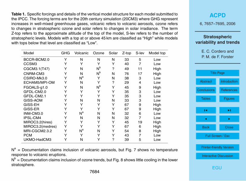
Table 1. Specific forcings and details of the vertical model structure for each model submitted tothe IPCC. The forcing terms are for the 20th century simulation (20CM3) where GHG representincreases in well-mixed greenhouse gases, volcanic refers to volcanic aerosols, ozone refersto changes in stratospheric ozone and solar refers to changes in solar irradiance. The termZ-top refers to the approximate altitude of the top of the model, S-lev refers to the number ofstratospheric levels. Models with a top at or above 45 km are classified as “High” while modelswith tops below that level are classified as “Low”.

Model GHG Volcanic Ozone Solar Z-top S-lev Model top

BCCR-BCM2.0 Y N N N 33 5 LowCCSM3 Y Y Y Y 40 7 LowCGCM3.1(T47) Y N Nb ? 49 11 HighCNRM-CM3 Y N Nb N 76 17 HighCSIRO-Mk3.0 Y Na Y N 38 3 LowECHAM5/MPI-OM Y N Y ? 29 4 LowFGOALS-g1.0 Y N Nb Y 45 9 HighGFDL-CM2.0 Y Y Y Y 35 3 LowGFDL-CM2.1 Y Y Y Y 35 3 LowGISS-AOM Y N N N 33 3 LowGISS-EH Y Y Y Y 67 9 HighGISS-ER Y Y Y Y 67 9 HighINM-CM3.0 Y Na N N 32 6 LowIPSL-CM4 Y N N N 32 7 LowMIROC3.2(hires) Y Y Y Y 45 19 HighMIROC3.2(medres) Y Y Y Y 67 6 HighMRI-CGCM2.3.2 Y Na N Y 54 8 HighPCM Y Y Y Y 43 7 LowUKMO-HadCM3 Y N Y ? 39 5 Low

Na = Documentation claims inclusion of volcanic aerosols, but Fig. 7 shows no temperatureresponse to volcanic eruptions.Nb = Documentation claims inclusion of ozone trends, but Fig. 8 shows little cooling in the lowerstratosphere.

7684





ACPD6, 7657–7695, 2006



Title Page



Tables Figures

J I

J I

Back Close

Full Screen / Esc



EGU

0.000

10.000

20.000

30.000

40.000

50.000

60.000

70.000

80.000BCCR-BCM2.0

BCC-CM1

CCSM3

CGCM3.1(T47)

CGCM3.1(T63)

CNRM-CM3

CSIRO-Mk3.0

ECHAM5/MPI-OM

ECHO-G

FGOALS-g1.0

GFDL-CM2.0

GFDL-CM2.1

GISS-AOM

GISS-EH

GISS-ER

INM-CM3.0

IPSL-CM4

MIROC3.2(hires)

MIROC3.2(medres)

MRI-CGCM2.3.2

PCM

UKMO-HadCM3

UKMO-HadGEM1

Alti

tude

(km

)

0.00

100.00

200.00

300.00

400.00

500.00

600.00

700.00

800.00

900.00

1000.00

Pres

sure

(hPa

)

Fig. 1. Approximate altitude of the vertical levels for models submitted to the IPCC AR4.

7685





ACPD6, 7657–7695, 2006



Title Page



Tables Figures

J I

J I

Back Close

Full Screen / Esc



EGU

200 220 240 260 280 300Temp (K)

1000

100

10A

ltit

ud

e (h

Pa)

bccr-bcm2.0ccsm3cgcm3.1-t47cnrm-cm3csiro-mk3.0echam5-mpi-omfgoals-g1.0gfdl-cm2.0gfdl-cm2.1giss-aomgiss-ehgiss-erinm-cm3.0ipsl-cm4miroc3.2-hmiroc3.2-mmri-cgcm2.3.2apcmukmo-hadcm3ukmo-hadgem1ncep1ncep1

-10 -5 0 5 10Model Temperature Bias (K)

1000

100

10

Alt

itu

de

(hP

a)

Fig. 2. Globally averaged temperature (left) and model temperature bias (right) between 1979–1999 for the climate models and the NCEP reanalysis. The lines identifying each model alter-nate between solid and dashed, so that for each color the first listed model uses a solid lineand the second listed model a dashed line. The gray shading in the model temperature biasplot shows NCEP plus and minus 2 standard deviations around the climatological mean.

7686





ACPD6, 7657–7695, 2006



Title Page



Tables Figures

J I

J I

Back Close

Full Screen / Esc



EGU

-50 0 50Latitude

200

220

240

260

280

300

Tem

p (

K)

bccr-bcm2.0ccsm3cgcm3.1-t47cnrm-cm3csiro-mk3.0echam5-mpi-omfgoals-g1.0gfdl-cm2.0gfdl-cm2.1giss-aomgiss-eh

giss-erinm-cm3.0ipsl-cm4miroc3.2-hmiroc3.2-mmri-cgcm2.3.2apcmukmo-hadcm3ukmo-hadgem1ncep1

bccr-bcm2.0ccsm3cgcm3.1-t47cnrm-cm3csiro-mk3.0echam5-mpi-omfgoals-g1.0gfdl-cm2.0gfdl-cm2.1giss-aomgiss-eh

giss-erinm-cm3.0ipsl-cm4miroc3.2-hmiroc3.2-mmri-cgcm2.3.2apcmukmo-hadcm3ukmo-hadgem1ncep1

Fig. 3. Zonally and annually averaged temperature at 500 hPa (upper) and 50 hPa (lower) be-tween 1979–1999 from the climate models and NCEP. The 2-σ variation in the NCEP reanalysisis shown in the heavy black vertical lines, and the colors are as in Fig. 2.

7687





ACPD6, 7657–7695, 2006



Title Page



Tables Figures

J I

J I

Back Close

Full Screen / Esc



EGU

70-90N: DJF

-15 -10 -5 0 5 10Difference (model - NCEP)

1000

100

10

Pre

ssu

re (

hP

a)

70-90N: DJF


1000

100

10

Pre

ssu

re (

hP

a)

70-90S: JJA


1000

100

10

Pre

ssu

re (

hP

a)

70-90S: JJA


1000

100

10

Pre

ssu

re (

hP

a)

Fig. 4. Zonally averaged temperature difference in K between the models and NCEP in the highlatitude winter hemisphere averaged between 1979–1999. Models with a high top are averagedtogether and displayed with a solid line and models with a low top are averaged together anddisplayed with a dashed line. The differences are computed for DJF (left) and JJA (right). Thegray shading indicates the 1 sigma standard deviation in the NCEP reanalysis.

7688





ACPD6, 7657–7695, 2006



Title Page



Tables Figures

J I

J I

Back Close

Full Screen / Esc



EGU

MayDec

June bccr-bcm2.0

MayDec

June ccsm3

MayDec

June cgcm3.1-t47

MayDec

June cnrm-cm3

MayDec

June csiro-mk3.0

MayDec

June echam5-mpi-om

MayDec

June fgoals-g1.0

MayDec

June gfdl-cm2.0

MayDec

June giss-eh

MayDec

June inm-cm3.0

MayDec

June ipsl-cm4

MayDec

June miroc3.2-h

MayDec

June mri-cgcm2.3.2a

MayDec

June pcm

MayDec

June ukmo-hadcm3

MayDec

June NCEP Reanalysis

-20 0 20 40 Zonal wind (m/s) at 60N and 50hPa

MayDec

June

Dec

JuneJan

bccr-bcm2.0

Dec

JuneJan

ccsm3

Dec

JuneJan

cgcm3.1-t47

Dec

JuneJan

cnrm-cm3

Dec

JuneJan

csiro-mk3.0

Dec

JuneJan

echam5-mpi-om

Dec

JuneJan

fgoals-g1.0

Dec

JuneJan

gfdl-cm2.0

Dec

JuneJan

giss-eh

Dec

JuneJan

inm-cm3.0

Dec

JuneJan

ipsl-cm4

Dec

JuneJan

miroc3.2-h

Dec

JuneJan

mri-cgcm2.3.2a

Dec

JuneJan

pcm

Dec

JuneJan

ukmo-hadcm3

Dec

JuneJan

NCEP Reanalysis-20 0 20 40 60

Zonal wind (m/s) at 60S and 50hPa

DecJune

Jan

Fig. 5. Time series of zonally averaged zonal wind at 60◦N (left) and 60◦ S (right) at 50 hPabetween the year 1979–1999 for a subset of the submitted IPCC models and the NCEP reanal-ysis. Each of the 20 years of data is plotted on top of each other and compared to the 20 yearmean NCEP reanalysis given in the black bold line.

7689





ACPD6, 7657–7695, 2006



Title Page



Tables Figures

J I

J I

Back Close

Full Screen / Esc



EGU

1950 1960 1970 1980 1990 2000Year

-2

-1

0

1

2

3

4T

emp

erat

ure

(K

)bccr-bcm2.0:-0.065*ccsm3:-0.28cgcm3.1-t47:-0.005cnrm-cm3:0.001csiro-mk3.0:-0.40*echam5-mpi-om:-0.33*fgoals-g1.0:-0.087*gfdl-cm2.0:-0.46*gfdl-cm2.1:-0.48*giss-aom:-0.16*giss-eh:-0.24*

giss-er:-0.25*inm-cm3.0:-0.10*ipsl-cm4:-0.13*miroc3.2-h:-0.43miroc3.2-m:-0.38mri-cgcm2.3.2a:-0.16*pcm:-0.26*ukmo-hadcm3:-0.61*RATPAC-0.47*HadAT:-0.47*

Fig. 6. Time series of globally averaged annual temperature anomaly averaged at 50 hPa. Thesolid vertical black lines indicate major volcanic eruptions and the bold lines (solid and dashed)represent the radiosonde observations from RATPAC-A and HadAT respectively. Next to eachmodel is the linear temperature trend in K decade−1 calculated between 1958–1999, and thelines alternate from solid to dashed as in Fig. 2. Models with statistically significant trends areindicated with asterisk (*) after the trend.

7690





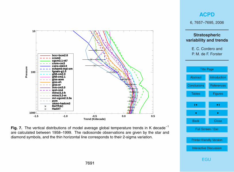
ACPD6, 7657–7695, 2006



Title Page



Tables Figures

J I

J I

Back Close

Full Screen / Esc



EGU

-1.5 -1.0 -0.5 0.0 0.5Trend (K/decade)

1000

100

10

Pre

ssu

re

HadATRATPACukmo-hadcm3pcmmri-cgcm2.3.2amiroc3.2-mmiroc3.2-hipsl-cm4inm-cm3.0giss-ergiss-ehgiss-aomgfdl-cm2.1gfdl-cm2.0fgoals-g1.0echam5-mpi-omcsiro-mk3.0cnrm-cm3cgcm3.1-t47ccsm3bccr-bcm2.0

HadATRATPACukmo-hadcm3pcmmri-cgcm2.3.2amiroc3.2-mmiroc3.2-hipsl-cm4inm-cm3.0giss-ergiss-ehgiss-aomgfdl-cm2.1gfdl-cm2.0fgoals-g1.0echam5-mpi-omcsiro-mk3.0cnrm-cm3cgcm3.1-t47ccsm3bccr-bcm2.0

Fig. 7. The vertical distributions of model average global temperature trends in K decade−1

are calculated between 1958–1999. The radiosonde observations are given by the star anddiamond symbols, and the thin horizontal line corresponds to their 2-sigma variation.

7691





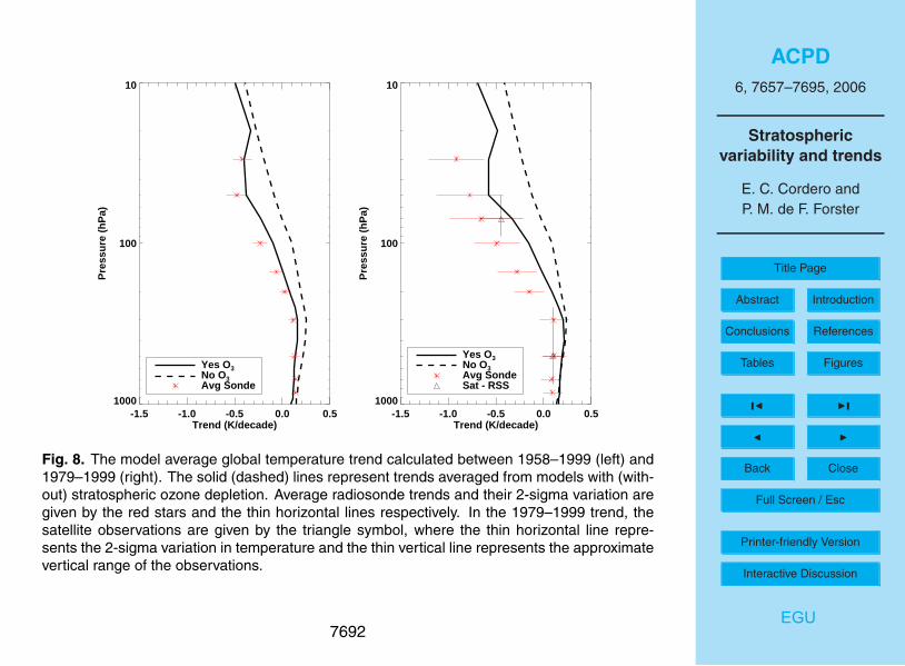
ACPD6, 7657–7695, 2006



Title Page



Tables Figures

J I

J I

Back Close

Full Screen / Esc



EGU

-1.5 -1.0 -0.5 0.0 0.5Trend (K/decade)

1000

100

10P

ress

ure

(h

Pa)

Avg Sonde No O3

Yes O3

-1.5 -1.0 -0.5 0.0 0.5Trend (K/decade)

1000

100

10

Pre

ssu

re (

hP

a)

Sat - RSSAvg Sonde No O3

Yes O3

Fig. 8. The model average global temperature trend calculated between 1958–1999 (left) and1979–1999 (right). The solid (dashed) lines represent trends averaged from models with (with-out) stratospheric ozone depletion. Average radiosonde trends and their 2-sigma variation aregiven by the red stars and the thin horizontal lines respectively. In the 1979–1999 trend, thesatellite observations are given by the triangle symbol, where the thin horizontal line repre-sents the 2-sigma variation in temperature and the thin vertical line represents the approximatevertical range of the observations.

7692





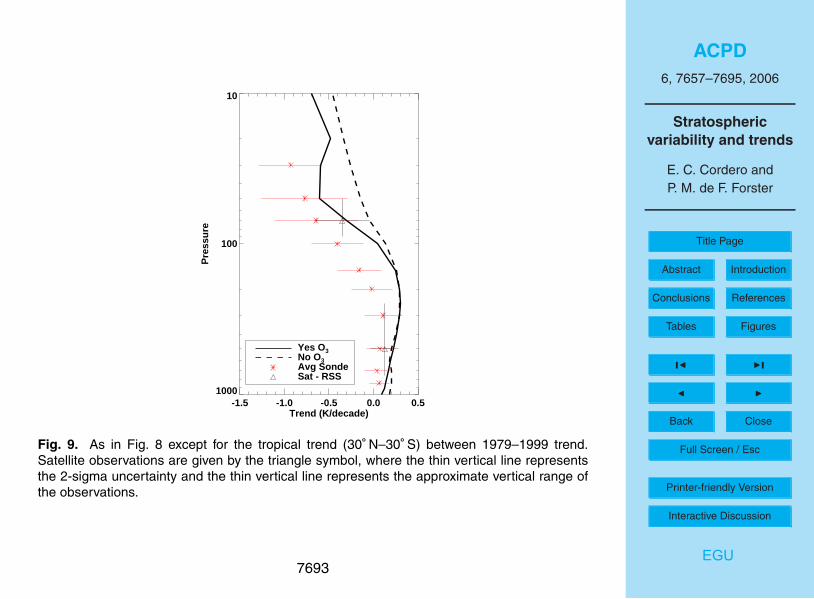
ACPD6, 7657–7695, 2006



Title Page



Tables Figures

J I

J I

Back Close

Full Screen / Esc



EGU

-1.5 -1.0 -0.5 0.0 0.5Trend (K/decade)

1000

100

10

Pre

ssu

re

Sat - RSSAvg Sonde No O3

Yes O3

Fig. 9. As in Fig. 8 except for the tropical trend (30◦ N–30◦ S) between 1979–1999 trend.Satellite observations are given by the triangle symbol, where the thin vertical line representsthe 2-sigma uncertainty and the thin vertical line represents the approximate vertical range ofthe observations.

7693





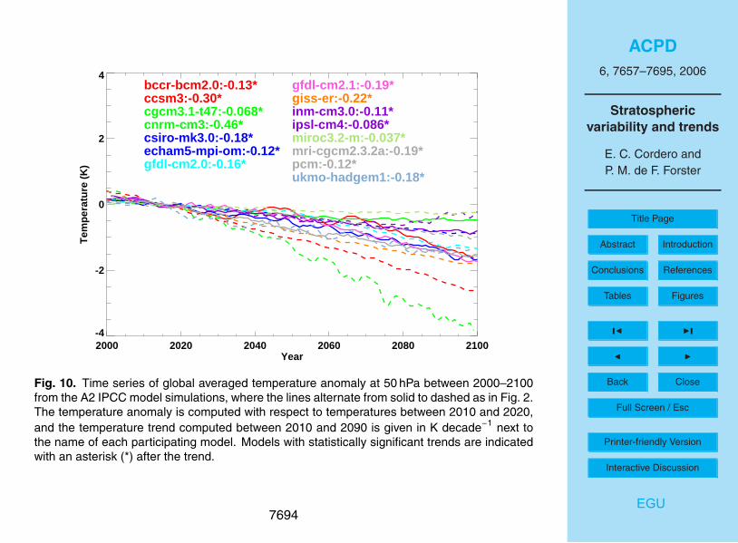
ACPD6, 7657–7695, 2006



Title Page



Tables Figures

J I

J I

Back Close

Full Screen / Esc



EGU

2000 2020 2040 2060 2080 2100Year

-4

-2

0

2

4T

emp

erat

ure

(K

)bccr-bcm2.0:-0.13*ccsm3:-0.30*cgcm3.1-t47:-0.068*cnrm-cm3:-0.46*csiro-mk3.0:-0.18*echam5-mpi-om:-0.12*gfdl-cm2.0:-0.16*

gfdl-cm2.1:-0.19*giss-er:-0.22*inm-cm3.0:-0.11*ipsl-cm4:-0.086*miroc3.2-m:-0.037*mri-cgcm2.3.2a:-0.19*pcm:-0.12*ukmo-hadgem1:-0.18*

Fig. 10. Time series of global averaged temperature anomaly at 50 hPa between 2000–2100from the A2 IPCC model simulations, where the lines alternate from solid to dashed as in Fig. 2.The temperature anomaly is computed with respect to temperatures between 2010 and 2020,and the temperature trend computed between 2010 and 2090 is given in K decade−1 next tothe name of each participating model. Models with statistically significant trends are indicatedwith an asterisk (*) after the trend.

7694





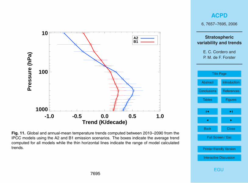
ACPD6, 7657–7695, 2006



Title Page



Tables Figures

J I

J I

Back Close

Full Screen / Esc



EGU

-1.0 -0.5 0.0 0.5 1.0Trend (K/decade)

1000

100

10P

ress

ure

(h

Pa)

A2B1

Fig. 11. Global and annual-mean temperature trends computed between 2010–2090 from theIPCC models using the A2 and B1 emission scenarios. The boxes indicate the average trendcomputed for all models while the thin horizontal lines indicate the range of model calculatedtrends.

7695





Documents

Stratospheric variability and trends in IPCC model … · Stratospheric variability and trends in ... Stratospheric variability and trends ... 20 Observational climatologies of temperature