Trend Filtering - Stanford Universityboyd/papers/pdf/l1_trend_filter.pdf · trend ﬁltering is a batch method for estimating the trend component from the whole history of observations.)

Copyright © by SIAM. Unauthorized reproduction of this article is prohibited.

SIAM REVIEW c! 2009 Society for Industrial and Applied MathematicsVol. 51, No. 2, pp. 339–360

!1 Trend Filtering!

Seung-Jean Kim†

Kwangmoo Koh†

Stephen Boyd†

Dimitry Gorinevsky†

Abstract. The problem of estimating underlying trends in time series data arises in a variety of disci-plines. In this paper we propose a variation on Hodrick–Prescott (H-P) filtering, a widelyused method for trend estimation. The proposed !1 trend filtering method substitutesa sum of absolute values (i.e., !1 norm) for the sum of squares used in H-P filtering topenalize variations in the estimated trend. The !1 trend filtering method produces trendestimates that are piecewise linear, and therefore it is well suited to analyzing time serieswith an underlying piecewise linear trend. The kinks, knots, or changes in slope of theestimated trend can be interpreted as abrupt changes or events in the underlying dynam-ics of the time series. Using specialized interior-point methods, !1 trend filtering can becarried out with not much more e!ort than H-P filtering; in particular, the number ofarithmetic operations required grows linearly with the number of data points. We describethe method and some of its basic properties and give some illustrative examples. We showhow the method is related to !1 regularization-based methods in sparse signal recovery andfeature selection, and we list some extensions of the basic method.

Key words. detrending, !1 regularization, Hodrick–Prescott filtering, piecewise linear fitting, sparsesignal recovery, feature selection, time series analysis, trend estimation

AMS subject classifications. 37M10, 62P99

DOI. 10.1137/070690274

1. Introduction.

1.1. Trend Filtering. We are given a scalar time series yt, t = 1, . . . , n, assumedto consist of an underlying slowly varying trend xt and a more rapidly varying randomcomponent zt. Our goal is to estimate the trend component xt or, equivalently, esti-mate the random component zt = yt ! xt. This can be considered as an optimizationproblem with two competing objectives: We want xt to be smooth, and we want zt

(our estimate of the random component, sometimes called the residual) to be small.In some contexts, estimating xt is called smoothing or filtering.

Trend filtering comes up in several applications and settings including macroeco-nomics (e.g., [52, 86]), geophysics (e.g., [1, 8, 9]), financial time series analysis (e.g.,[97]), social sciences (e.g., [66]), revenue management (e.g., [91]), and biological andmedical sciences (e.g., [43, 68]). Many trend filtering methods have been proposed,

!Received by the editors May 2, 2007; accepted for publication (in revised form) May 28, 2008;published electronically May 4, 2009. This work was funded in part by the Precourt Institute onEnergy E"ciency, by Army award W911NF-07-1-0029, by NSF award 0529426, by NASA awardNNX07AEIIA, by AFOSR award FA9550-06-1-0514, and by AFOSR award FA9550-06-1-0312.

http://www.siam.org/journals/sirev/51-2/69027.html†Information Systems Laboratory, Electrical Engineering Department, Stanford University,

Stanford, CA 94305-9510 ([email protected], [email protected], [email protected], [email protected]).

339


340 SEUNG-JEAN KIM, KWANGMOO KOH, STEPHEN BOYD, AND DIMITRY GORINEVSKY

including Hodrick–Prescott (H-P) filtering [52, 64], moving average filtering [75], expo-nential smoothing [70], bandpass filtering [21, 4], smoothing splines [81], de-trendingvia rational square-wave filters [79], a jump process approach [106], median filtering[101], a linear programming (LP) approach with fixed kink points [72], and wavelettransform analysis [23]. (All these methods except for the jump process approach, theLP approach, and median filtering are linear filtering methods; see [4] for a surveyof linear filtering methods in trend estimation.) The most widely used methods aremoving average filtering, exponential smoothing, and H-P filtering, which is especiallypopular in economics and related disciplines due to its application to business cycletheory [52]. The idea behind H-P filtering can be found in several fields and can betraced back at least to work in 1961 by Leser [64] in statistics.

1.2. !1 Trend Filtering. In this paper we propose !1 trend filtering, a variationon H-P filtering which substitutes a sum of absolute values (i.e., an !1 norm) for thesum of squares used in H-P filtering to penalize variations in the estimated trend.(The term “filtering” is used in analogy with “H-P filtering.” Like H-P filtering, !1trend filtering is a batch method for estimating the trend component from the wholehistory of observations.)

We will see that the proposed !1 trend filter method shares many properties withthe H-P filter and has the same (linear) computational complexity. The principaldi!erence is that the !1 trend filter produces trend estimates that are smooth in thesense of being piecewise linear. The !1 trend filter is thus well suited to analyzingtime series with an underlying piecewise linear trend. The kinks, knots, or changesin slope of the estimated trend can be interpreted as abrupt changes or events inthe underlying dynamics of the time series; the !1 trend filter can be interpretedas detecting or estimating changes in an underlying linear trend. Using specializedinterior-point methods, !1 trend filtering can be carried out with not much more e!ortthan H-P filtering; in particular, the number of arithmetic operations required growslinearly with the number of data points.

1.3. Outline. In the next section we set up our notation and give a brief summaryof H-P filtering, listing some properties for later comparison with our proposed !1trend filter. The !1 trend filter is described in section 3 and compared to the H-Pfilter. We give some illustrative examples in section 4.

In section 5 we give the optimality condition for the underlying optimizationproblem that defines the !1 trend filter, and we use it to derive some of the propertiesgiven in section 3. We also derive a Lagrange dual problem that is interesting on itsown and is also used in a primal-dual interior-point method we describe in section 6.We list a number of extensions of the basic idea in section 7.

2. Hodrick–Prescott Filtering. In H-P filtering, the trend estimate xt is chosento minimize the weighted sum objective function

(1) (1/2)n

!

t=1

(yt ! xt)2 + "n"1!

t=2

(xt"1 ! 2xt + xt+1)2,

where " " 0 is the regularization parameter used to control the trade-o! betweensmoothness of xt and the size of the residual yt ! xt. The first term in the objectivefunction measures the size of the residual; the second term measures the smoothnessof the estimated trend. The argument appearing in the second term, xt"1!2xt+xt+1,is the second di!erence of the time series at time t; it is zero when and only when the


!1 TREND FILTERING 341

three points xt"1, xt, xt+1 are on a line. The second term in the objective is zero ifand only if xt is a"ne, i.e., has the form xt = # + $t for some constants # and $.(In other words, the graph of xt is a straight line.) The weighted sum objective (1)is strictly convex and coercive in x, and so has a unique minimizer, which we denotexhp.

We can write the objective (1) as

(1/2)#y ! x#22 + "#Dx#2

2,

where x = (x1, . . . , xn) $ Rn, y = (y1, . . . , yn) $ Rn, #u#2 = ("

i u2i )1/2 is the

Euclidean or !2 norm, and D $ R(n"2)#n is the second-order di!erence matrix

(2) D =

#

$

$

$

$

$

%

1 !2 11 !2 1

. . . . . . . . .1 !2 1

1 !2 1

&

'

'

'

'

'

(

.

(D is Toeplitz with first row [ 1 !2 1 0 · · · 0 ]; entries not shown above are zero.)The H-P trend estimate is

(3) xhp = (I + 2"DT D)"1y.

H-P filtering is supported in several standard software packages for statistical dataanalysis, e.g., SAS, R, and Stata.

We list some basic properties of H-P filtering, which we refer to later when wecompare it to our proposed trend estimation method.

• Linear computational complexity. The H-P estimated trend xhp in (3) can becomputed in O(n) arithmetic operations, since D is tridiagonal.

• Linearity. From (3) we see that the H-P estimated trend xhp is a linearfunction of the time series data y.

• Convergence to original data as " % 0. The relative fitting error satisfies theinequality

(4)#y ! xhp#2

#y#2& 32"

1 + 32".

This shows that as the regularization parameter " decreases to zero, xhp

converges to the original time series data y.• Convergence to best a"ne fit as " % '. As " % ', the H-P estimated trend

converges to the best a"ne (straight-line) fit to the time series data,

xba = #ba + $bat,

with intercept and slope

#ba ="n

t=1 t2"n

t=1 yt !"n

t=1 t"n

t=1 tyt

n"n

t=1 t2 ! ("n

t=1 t)2,

$ba =n

"nt=1 tyt !

"nt=1 t

"nt=1 yt

n"n

t=1 t2 ! ("n

t=1 t)2.



• Commutability with a"ne adjustment. We can change the order of H-P filter-ing and a"ne adjustment of the original time series data, without a!ect: Forany # and $, the H-P trend estimate of the time series data yt = yt!#!$t isxhp

t = xhpt !#! $t. (A special case of linear adjustment is linear detrending,

with # = #ba, $ = $ba, which corresponds to subtracting the best a"ne fitfrom the original data.)

• Regularization path. The H-P trend estimate xhp is a smooth function of theregularization parameter ", as it varies over [0,'). As " decreases to zero,xhp converges to the original data y; as " increases, xhp becomes smoother,and converges to xba, the best a"ne fit to the time series data.

We can derive the relative fitting error inequality (4) as follows. From the opti-mality condition y ! xhp = "DT Dxhp we obtain

y ! xhp = 2"DT D(I + 2"DT D)"1y.

The spectral norm of D is no more than 4:

#Dx#2 = #x1:n"2 ! 2x2:n"1 + x3:n#2 & #x1:n"2#2 + 2#x2:n"1#2 + #x3:n#2 & 4#x#2,

where xi:j = (xi, . . . , xj). The eigenvalues of DT D lie between 0 and 16, so theeigenvalues of 2"DT D(I + 2"DT D)"1 lie between 0 and 32"/(1 + 32"). It followsthat

#y ! xhp#2 & (32"/(1 + 32"))#y#2.

3. !1 Trend Filtering. We propose the following variation on H-P filtering, whichwe call !1 trend filtering. We choose the trend estimate as the minimizer of theweighted sum objective function

(5) (1/2)n

!

t=1

(yt ! xt)2 + "n"1!

t=2

|xt"1 ! 2xt + xt+1|,

which can be written in matrix form as

(1/2)#y ! x#22 + "#Dx#1,

where #u#1 ="

i |ui| denotes the !1 norm of the vector u. As in H-P filtering, " isa nonnegative parameter used to control the trade-o! between smoothness of x andsize of the residual. The weighted sum objective (1) is strictly convex and coercive inx and so has a unique minimizer, which we denote xlt. (The superscript “lt” standsfor “!1 trend.”)

We list some basic properties of !1 trend filtering, pointing out similarities anddi!erences with H-P filtering.

• Linear computational complexity. There is no analytic formula or expressionfor xlt, analogous to (3). But like xhp, xlt can be computed numerically inO(n) arithmetic operations. (We describe an e"cient method for computingxlt in section 6. Its worst-case complexity is O(n1.5), but practically itscomputational e!ort is linear in n.)

• Nonlinearity. The !1 trend estimate xlt is not a linear function of the originaldata y. (In contrast, xhp is a linear function of y.)



• Convergence to original data as " % 0. The maximum fitting error satisfiesthe bound

(6) #y ! xlt#$ & 4",

where #u#$ = maxi |ui| denotes the !$ norm of the vector u. (Cf. theanalogous bound for H-P trend estimation, given in (4).) This implies thatxlt % y as " % 0.

• Finite convergence to best a"ne fit as " % '. As in H-P filtering, xlt % xba

as " % '. For !1 trend estimation, however, the convergence occurs for afinite value of ",

(7) "max = #(DDT )"1Dy#$.

For " " "max, we have xlt = xba. (In contrast, xhp % xba only in thelimit as " % '.) This maximum value "max is readily computed with O(n)arithmetic steps. (The derivation is given in section 5.1.)

• Commutability with a"ne adjustment. As in H-P filtering, we can swap theorder of a"ne adjustment and trend filtering, without a!ect.

• Piecewise-linear regularization path. The !1 trend estimate xlt is a piecewise-linear function of the regularization parameter ", as it varies over [0,'):There are values "1, . . . ,"k, with 0 = "k < · · · < "1 = "max, for which

xlt ="i ! "

"i ! "i+1x(i+1) +

"! "i+1

"i ! "i+1x(i), "i+1 & " & "i, i = 1, . . . , k ! 1,

where x(i) is xlt with " = "i. (So x(1) = xba, x(k) = y.)• Linear extension property. Let xlt denote the !1 trend estimate for (y1, . . . , yn+1).

There is an interval [l, u], with l < u, for which

xlt = (xlt, 2xltn ! xlt

n"1),

provided yn+1 $ [u, l]. In other words, if the new observation is inside aninterval, the !1 trend estimate linearly extends the last a"ne segment.

3.1. Piecewise Linearity. The basic reason the !1 trend estimate xlt might bepreferred over the H-P trend estimate xhp is that it is piecewise linear in t: There are(integer) times 1 = t1 < t2 < · · · < tp"1 < tp = n for which

(8) xltt = #k + $kt, tk & t & tk+1, k = 1, . . . , p ! 1.

In other words, over each (integer) interval [ti, ti+1], xlt is an a"ne function of t. Wecan interpret #k and $k as the local intercept and slope in the kth interval. Theselocal trend parameters are not independent: they must give consistent values for xlt

at the join or kink points, i.e.,

#k + $ktk+1 = #k+1 + $k+1tk+1, k = 1, . . . , p ! 1.

The points t2, . . . , tp"1 are called kink points. We say that xlt is piecewise linear withp! 2 kink points. (The kink point tk can be eliminated if #k = #k"1, so we generallyassume that #k (= #k"1.)

In one extreme case, we have p = 2, which corresponds to no kink points. In thiscase t1 = 1, t2 = n, and xlt = xba is a"ne. In the other extreme case, there is a kink



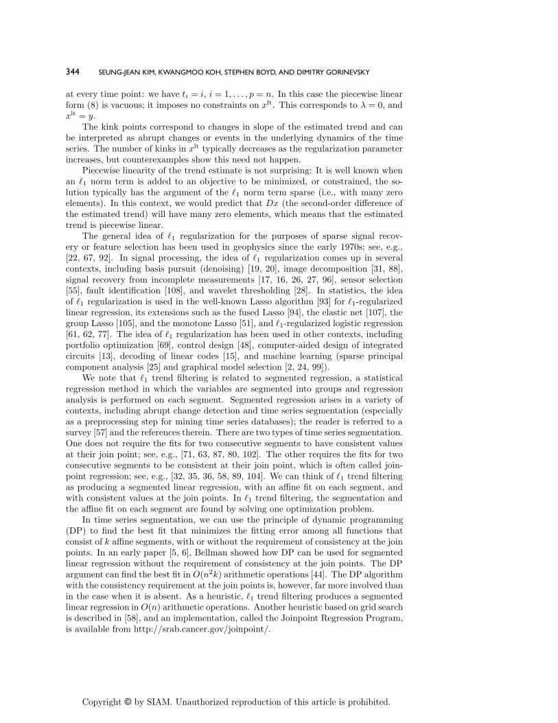
at every time point: we have ti = i, i = 1, . . . , p = n. In this case the piecewise linearform (8) is vacuous; it imposes no constraints on xlt. This corresponds to " = 0, andxlt = y.

The kink points correspond to changes in slope of the estimated trend and canbe interpreted as abrupt changes or events in the underlying dynamics of the timeseries. The number of kinks in xlt typically decreases as the regularization parameterincreases, but counterexamples show this need not happen.

Piecewise linearity of the trend estimate is not surprising: It is well known whenan !1 norm term is added to an objective to be minimized, or constrained, the so-lution typically has the argument of the !1 norm term sparse (i.e., with many zeroelements). In this context, we would predict that Dx (the second-order di!erence ofthe estimated trend) will have many zero elements, which means that the estimatedtrend is piecewise linear.

The general idea of !1 regularization for the purposes of sparse signal recov-ery or feature selection has been used in geophysics since the early 1970s; see, e.g.,[22, 67, 92]. In signal processing, the idea of !1 regularization comes up in severalcontexts, including basis pursuit (denoising) [19, 20], image decomposition [31, 88],signal recovery from incomplete measurements [17, 16, 26, 27, 96], sensor selection[55], fault identification [108], and wavelet thresholding [28]. In statistics, the ideaof !1 regularization is used in the well-known Lasso algorithm [93] for !1-regularizedlinear regression, its extensions such as the fused Lasso [94], the elastic net [107], thegroup Lasso [105], and the monotone Lasso [51], and !1-regularized logistic regression[61, 62, 77]. The idea of !1 regularization has been used in other contexts, includingportfolio optimization [69], control design [48], computer-aided design of integratedcircuits [13], decoding of linear codes [15], and machine learning (sparse principalcomponent analysis [25] and graphical model selection [2, 24, 99]).

We note that !1 trend filtering is related to segmented regression, a statisticalregression method in which the variables are segmented into groups and regressionanalysis is performed on each segment. Segmented regression arises in a variety ofcontexts, including abrupt change detection and time series segmentation (especiallyas a preprocessing step for mining time series databases); the reader is referred to asurvey [57] and the references therein. There are two types of time series segmentation.One does not require the fits for two consecutive segments to have consistent valuesat their join point; see, e.g., [71, 63, 87, 80, 102]. The other requires the fits for twoconsecutive segments to be consistent at their join point, which is often called join-point regression; see, e.g., [32, 35, 36, 58, 89, 104]. We can think of !1 trend filteringas producing a segmented linear regression, with an a"ne fit on each segment, andwith consistent values at the join points. In !1 trend filtering, the segmentation andthe a"ne fit on each segment are found by solving one optimization problem.

In time series segmentation, we can use the principle of dynamic programming(DP) to find the best fit that minimizes the fitting error among all functions thatconsist of k a"ne segments, with or without the requirement of consistency at the joinpoints. In an early paper [5, 6], Bellman showed how DP can be used for segmentedlinear regression without the requirement of consistency at the join points. The DPargument can find the best fit in O(n2k) arithmetic operations [44]. The DP algorithmwith the consistency requirement at the join points is, however, far more involved thanin the case when it is absent. As a heuristic, !1 trend filtering produces a segmentedlinear regression in O(n) arithmetic operations. Another heuristic based on grid searchis described in [58], and an implementation, called the Joinpoint Regression Program,is available from http://srab.cancer.gov/joinpoint/.



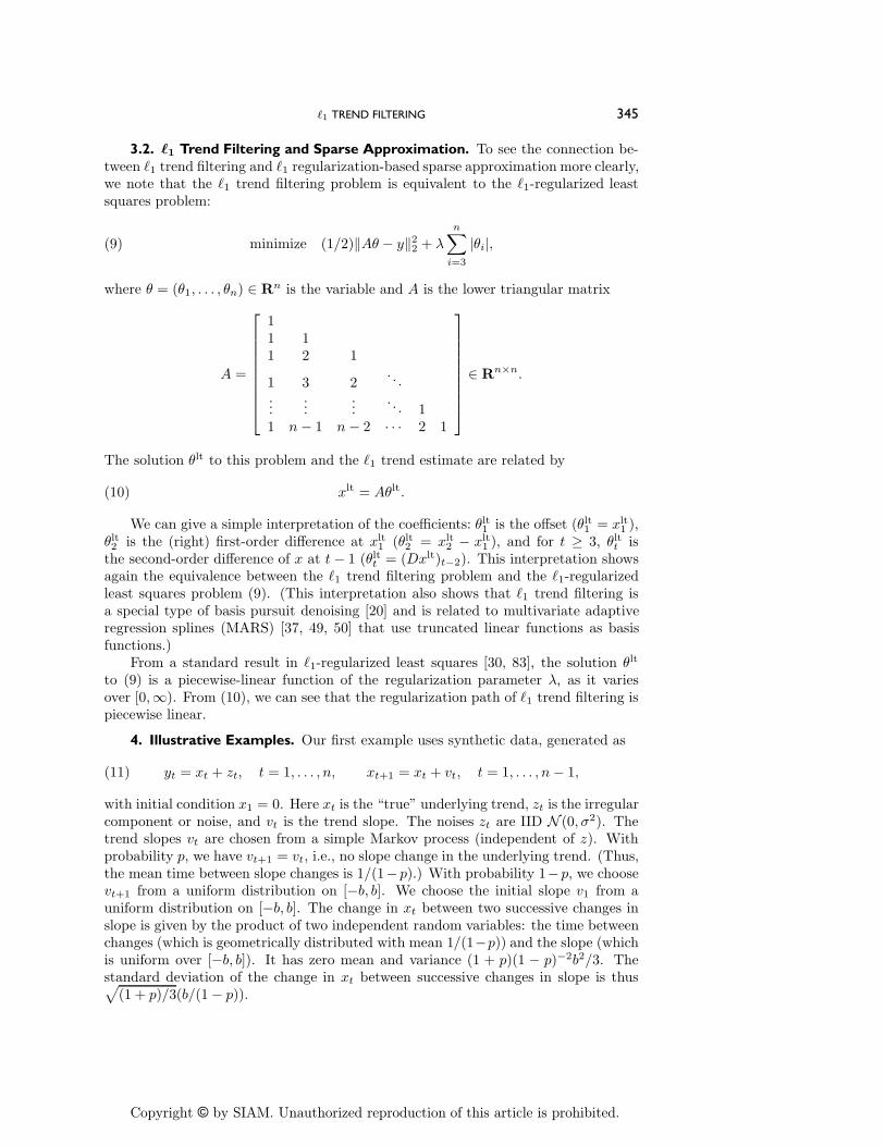
3.2. !1 Trend Filtering and Sparse Approximation. To see the connection be-tween !1 trend filtering and !1 regularization-based sparse approximation more clearly,we note that the !1 trend filtering problem is equivalent to the !1-regularized leastsquares problem:

(9) minimize (1/2)#A% ! y#22 + "

n!

i=3

|%i|,

where % = (%1, . . . , %n) $ Rn is the variable and A is the lower triangular matrix

A =

#

$

$

$

$

$

$

$

$

%

11 11 2 1

1 3 2. . .

......

.... . . 1

1 n ! 1 n ! 2 · · · 2 1

&

'

'

'

'

'

'

'

'

(

$ Rn#n.

The solution %lt to this problem and the !1 trend estimate are related by

(10) xlt = A%lt.

We can give a simple interpretation of the coe"cients: %lt1 is the o!set (%lt

1 = xlt1 ),

%lt2 is the (right) first-order di!erence at xlt

1 (%lt2 = xlt

2 ! xlt1 ), and for t " 3, %lt

t isthe second-order di!erence of x at t ! 1 (%lt

t = (Dxlt)t"2). This interpretation showsagain the equivalence between the !1 trend filtering problem and the !1-regularizedleast squares problem (9). (This interpretation also shows that !1 trend filtering isa special type of basis pursuit denoising [20] and is related to multivariate adaptiveregression splines (MARS) [37, 49, 50] that use truncated linear functions as basisfunctions.)

From a standard result in !1-regularized least squares [30, 83], the solution %lt

to (9) is a piecewise-linear function of the regularization parameter ", as it variesover [0,'). From (10), we can see that the regularization path of !1 trend filtering ispiecewise linear.

4. Illustrative Examples. Our first example uses synthetic data, generated as

yt = xt + zt, t = 1, . . . , n, xt+1 = xt + vt, t = 1, . . . , n ! 1,(11)

with initial condition x1 = 0. Here xt is the “true” underlying trend, zt is the irregularcomponent or noise, and vt is the trend slope. The noises zt are IID N (0,&2). Thetrend slopes vt are chosen from a simple Markov process (independent of z). Withprobability p, we have vt+1 = vt, i.e., no slope change in the underlying trend. (Thus,the mean time between slope changes is 1/(1!p).) With probability 1!p, we choosevt+1 from a uniform distribution on [!b, b]. We choose the initial slope v1 from auniform distribution on [!b, b]. The change in xt between two successive changes inslope is given by the product of two independent random variables: the time betweenchanges (which is geometrically distributed with mean 1/(1!p)) and the slope (whichis uniform over [!b, b]). It has zero mean and variance (1 + p)(1 ! p)"2b2/3. Thestandard deviation of the change in xt between successive changes in slope is thus)

(1 + p)/3(b/(1 ! p)).



For our example, we use the parameter values

n = 1000, p = 0.99, & = 20, b = 0.5.

Thus, the mean time between slope changes is 100, and the standard deviation of thechange in xt between slope changes is 40.7. The particular sample we generated had8 changes in slope.

The !1 trend estimates were computed using two solvers: cvx [42], a MATLAB-based modeling system for convex optimization (which calls SDPT3 [95] or SeDuMi[90], a MATLAB-based solver for convex problems), and a C implementation of thespecialized primal-dual interior-point method described in section 6. The run timeson a 3GHz Pentium IV were around a few seconds and 0.01 seconds, respectively.

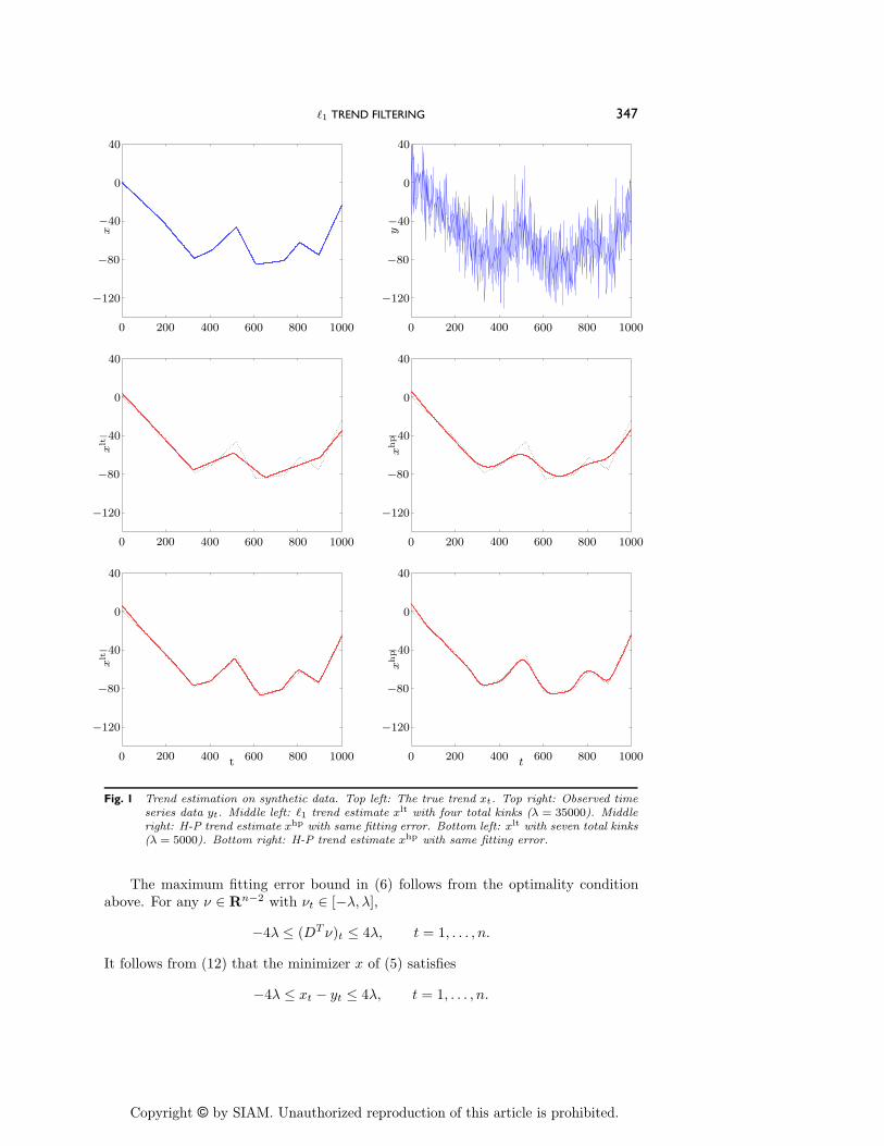
The results are shown in Figure 1. The top left plot shows the true trend xt, andthe top right plot shows the noise corrupted time series yt. In the middle left plot,we show xlt for " = 35000, which results in 4 kink points in the estimated trend.The middle right plot shows the H-P trend estimate with " adjusted to give the samefitting error as xlt, i.e., #y! xlt#2 = #y! xhp#2. Even though xlt is not a particularlygood estimate of xt, it has identified some of the slope change points fairly well. Thebottom left plot shows xlt for " = 5000, which yields 7 kink points in xlt. The bottomright plot shows xhp, with the same fitting error. In this case the estimate of theunderlying trend is quite good. Note that the trend estimation error for xlt is betterthan xhp, especially around the kink points.

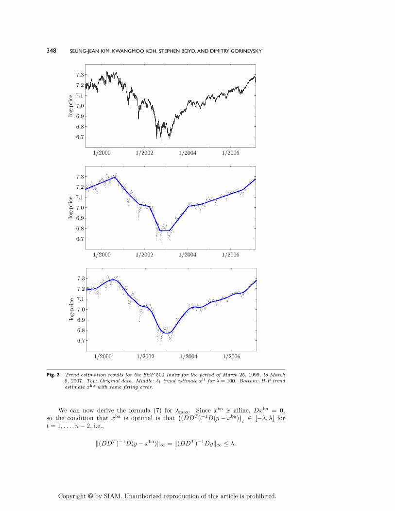
Our next example uses real data, 2000 consecutive daily closing values of theS&P 500 Index, from March 25, 1999, to March 9, 2007, after logarithmic transform.The data are shown in the top plot of Figure 2. In the middle plot, we show xlt for" = 100, which results in 8 kink points in the estimated trend. The bottom plotshows the H-P trend estimate with the same fitting error.

In this example (in contrast to the previous one) we cannot say that the !1 trendestimate is better than the H-P trend estimate. Each of the two trend estimates is asmoothed version of the original data; by construction, they have the same !2 fittingerror. If for some reason you believe that the (log of the) S&P 500 Index is driven byan underlying trend that is piecewise linear, you might prefer the !1 trend estimateover the H-P trend estimate.

5. Optimality Condition and Dual Problem.

5.1. Optimality Condition. The objective function (5) of the !1 trend filteringproblem is convex but not di!erentiable, so we use a first-order optimality conditionbased on subdi!erential calculus. We obtain the following necessary and su"cientcondition for x to minimize (5): there exists ' $ Rn such that

(12) y ! x = DT ', 't $

*

+

,

{+"}, (Dx)t > 0,{!"}, (Dx)t < 0,[!","], (Dx)t = 0,

t = 1, . . . , n ! 2.

(Here, we use the chain rule for subdi!erentials: If f is convex, then the subdi!erentialof h(x) = f(Ax + b) is given by (h(x) = AT(f(Ax + b). See, e.g., [7, Prop. B.24]or [10, Chap. 2] for more on subdi!erential calculus.) Since DDT is invertible, theoptimality condition (12) can be written as

-

(DDT )"1D(y ! x).

t$

*

+

,

{+"}, (Dx)t > 0,{!"}, (Dx)t < 0,[!", "], (Dx)t = 0,

t = 1, . . . , n ! 2.


!1 TREND FILTERING 347x

0 200 400 600 800 1000

!120

!80

!40

0

40

0 200 400 600 800 1000

!120

!80

!40

0

40

y

0 200 400 600 800 1000

!120

!80

!40

0

40

xlt

0 200 400 600 800 1000

!120

!80

!40

0

40

xhp

0 200 400 600 800 1000

!120

!80

!40

0

40

xlt

t 0 200 400 600 800 1000

!120

!80

!40

0

40

xhp

t

Fig. 1 Trend estimation on synthetic data. Top left: The true trend xt. Top right: Observed timeseries data yt. Middle left: !1 trend estimate xlt with four total kinks (" = 35000). Middleright: H-P trend estimate xhp with same fitting error. Bottom left: xlt with seven total kinks(" = 5000). Bottom right: H-P trend estimate xhp with same fitting error.

The maximum fitting error bound in (6) follows from the optimality conditionabove. For any ' $ Rn"2 with 't $ [!","],

!4" & (DT ')t & 4", t = 1, . . . , n.

It follows from (12) that the minimizer x of (5) satisfies

!4" & xt ! yt & 4", t = 1, . . . , n.



log-

price

1/2000 1/2002 1/2004 1/2006

6.7

6.8

6.9

7.0

7.1

7.2

7.3lo

g-price

1/2000 1/2002 1/2004 1/2006

6.7

6.8

6.9

7.0

7.1

7.2

7.3

log-

price

1/2000 1/2002 1/2004 1/2006

6.7

6.8

6.9

7.0

7.1

7.2

7.3

Fig. 2 Trend estimation results for the S&P 500 Index for the period of March 25, 1999, to March9, 2007. Top: Original data. Middle: !1 trend estimate xlt for " = 100. Bottom: H-P trendestimate xhp with same fitting error.

We can now derive the formula (7) for "max. Since xba is a"ne, Dxba = 0,so the condition that xba is optimal is that

-

(DDT )"1D(y ! xba).

t$ [!","] for

t = 1, . . . , n ! 2, i.e.,

#(DDT )"1D(y ! xba)#$ = #(DDT )"1Dy#$ & ".



We can use the optimality condition (12) to see whether the linear extensionproperty holds for a new observation yn+1. From the optimality condition (12), wecan see that if yn+1 satisfies

/

/

/

/

(DDT )"1D

01

yyn+1

2

!1

xlt

2xltn ! xlt

n"1

23/

/

/

/

$& ",

where D $ R(n"1)#(n+1) is the second-order di!erence matrix on Rn+1, then the!1 trend estimate for (y, yn+1) is given by (xlt, 2xlt

n ! xltn"1) $ Rn+1. From this

inequality, we can easily find the bounds l and u such that if l & yn+1 & u, then thelinear extension property holds.

5.2. Dual Problem. To derive a Lagrange dual of the primal problem of min-imizing (5), we first introduce a new variable z $ Rn"2, as well as a new equalityconstraint z = Dx, to obtain the equivalent formulation

minimize (1/2)#y ! x#22 + "#z#1

subject to z = Dx.

Associating a dual variable ' $ Rn"2 with the equality constraint, the Lagrangian is

L(x, z, ') = (1/2)#y ! x#22 + "#z#1 + 'T (Dx ! z).

The dual function is

infx,z

L(x, z, ') =4

!(1/2)'T DDT ' + yT DT ', !"1 & ' & "1,!' otherwise.

The dual problem is

(13) minimize g(') = (1/2)'T DDT ' ! yT DT 'subject to !"1 & ' & "1.

(Here a & b means ai & bi for all i.) The dual problem (13) is a (convex) quadraticprogram (QP) with variable ' $ Rn"2. We say that ' $ Rn"2 is strictly dual feasibleif it satisfies !"1 < ' < "1.

From the solution 'lt of the dual (13), we can recover the !1 trend estimate via

(14) xlt = y ! DT 'lt.

6. A Primal-Dual Interior-Point Method. The QP (13) can be solved by stan-dard convex optimization methods, including general interior-point methods [12, 73,74, 103] and more specialized methods such as path following [76, 30]. These methodscan exploit the special structure of the problem, i.e., the bandedness of the quadraticform in the objective, to solve the problem very e"ciently. To see how this can bedone, we describe a simple primal-dual method in this section. For more detail onthese (and related) methods, see, e.g., [12, section 11.7] or [103].

The worst-case number of iterations in primal-dual interior-point methods for theQP (13) is O(n1/2) [73]. In practice, primal-dual interior-point methods solve QPs ina number of iterations that is just a few tens, almost independent of the problem sizeor data. Each iteration is dominated by the cost of computing the search direction,which, if done correctly for the particular QP (13), is O(n). It follows that the overall



complexity is O(n), the same as for solving the H-P filtering problem (but with alarger constant hidden in the O(n) notation).

The search direction is the Newton step for the system of nonlinear equations

(15) rt(', µ1, µ2) = 0,

where t > 0 is a parameter and

rt(', µ1, µ2) =1

rdual

rcent

2

=1

)g(') + D(' ! "1)T µ1 ! D(' + "1)T µ2

!µ1(' ! "1) + µ2(' + "1) ! (1/t)1

2

(16)

is the residual. (The first component is the dual feasibility residual, and the secondis the centering residual.) Here µ1, µ2 $ Rn"2 are (positive) dual variables for theinequality constraints in (13), and ' is strictly dual feasible. As t % ', rt(', µ1, µ2) =0 reduces to the Karush–Kuhn–Tucker (KKT) condition for the QP (13). The basicidea is to take Newton steps for solving the set of nonlinear equations rt(', µ1, µ2) = 0for a sequence of increasing values of t.

The Newton step is characterized by

rt(' +#', µ1 +#µ1, µ1 +#µ1) * rt(', µ1, µ2) + Drt(', µ1, µ2)(#',#µ1,#µ2) = 0,

where Drt is the derivative (Jacobian) of rt. This can be written as#

%

DDT I !II J1 0!I 0 J2

&

(

#

%

#'#µ1

#µ2

&

( = !

#

%

DDT z ! Dy + µ1 ! µ2

f1 + (1/t) diag(µ1)"11f2 + (1/t) diag(µ2)"11

&

( ,(17)

where

f1 = ' ! "1 $ Rn"2,

f2 = !' ! "1 $ Rn"2,

Ji = diag(µi)"1 diag(fi) $ R(n"2)#(n"2).

(Here diag(w) is the diagonal matrix with diagonal entries w.) By eliminating(#µ1,#µ2), we obtain the reduced system-

DDT ! J"11 J"1

2

.

#' = !-

DDT ' ! Dy ! (1/t) diag(f1)"11 + (1/t) diag(f2)"11.

.

The matrix DDT !J"11 J"1

2 is banded (with bandwidth 5) so we can solve this reducedsystem in O(n) arithmetic operations. The other two components of the search step,#µ1 and #µ2, can be computed as

#µ1 = !-

µ1 + (1/t) diag(f1)"11 + J"11 d'

.

,

#µ2 = !-

µ2 + (1/t) diag(f2)"11! J"12 d'

.

in O(n) arithmetic operations (since the matrices J1 and J2 are diagonal).A C implementation of a primal-dual interior-point method for !1 trend filtering

is available online from www.stanford.edu/˜boyd/l1 tf. For a typical problem withn = 10000 data points, it computes xlt in around one second on a 3GHz Pentium IV.Problems with one million data points require around 100 seconds, consistent withlinear computational complexity in n.



7. Extensions and Variations. The basic !1 trend estimation method describedabove can be extended in many ways, some of which we describe here. In each case,the computation reduces to solving one or a few convex optimization problems, andso is quite tractable; the interior-point method described above is readily extended tohandle these problems.

7.1. Polishing. One standard trick is to use the basic !1 filtering problem as amethod to identify the kink points in the estimated trend. Once the kinks points{t1, . . . , tp} are identified, we use a standard least-squares method to fit the data overall piecewise-linear functions with the given kinks points:

minimizep"1!

k=1

!

tk%t%tk+1

#y ! #k ! $kt#22

subject to #k + $ktk+1 = #k+1 + $k+1tk+1, k = 1, . . . , p ! 2,

where the variables are the local trend parameters #k and $k. This technique isdescribed (in another context) in, e.g., [12, sect. 6.5].

7.2. Iterative Weighted !1 Heuristic. The basic !1 trend filtering method isequivalent to

(18) minimize #Dx#1

subject to #y ! x#2 & s,

with an appropriate choice of parameter s. In this formulation, we minimize #Dx#1

(our measure of smoothness of the estimated trend) subject to a budget on residualnorm. This problem can be considered a heuristic for the problem of finding thepiecewise-linear trend with the smallest number of kinks, subject to a budget onresidual norm:

minimize card(Dx)subject to #y ! x#2 & s,

where card(z) is the number of nonzero elements in a vector z. Solving this problemexactly is intractable; all known methods require an exhaustive combinatorial searchover all—or at least very many—possible combinations of kink points.

The standard heuristic for solving this problem is to replace card(Dx) with #Dx#1,which gives us our basic !1 trend filter, i.e., the solution to (18). This basic methodcan be improved by an iterative method that varies the individual weights on thesecond-order di!erences in xt. We start by solving (18). We then define a weightvector as

wt := 1/()+ |(Dx)t|), t = 1, . . . , n ! 2,

where ) is a small positive constant. This assigns the largest weight, 1/), when(Dx)t = 0; it assigns large weight when |(Dx)t| is small; and it assigns relativelysmall weight when |(Dx)t| is larger. We then recompute xt as the solution of problem

minimize # diag(w)Dx#1

subject to #y ! x#2 & s.

We then update the weights as above and repeat.



This iteration typically converges in 10 or fewer steps. It often gives a modestdecrease in the number of kink points card(Dx), for the same residual, compared tothe basic !1 trend estimation method. The idea behind this heuristic has been usedin portfolio optimization with transaction costs [69], where an interpretation of theheuristic for cardinality minimization is given. The reader is referred to [18] for amore extensive discussion on the iterative heuristic.

7.3. Convex Constraints and Penalty Functions. We can add convex constraintson the estimated trend, or use a more general convex penalty function to measure theresidual. In both cases, the resulting trend estimation problem is convex, and there-fore tractable. We list a few examples here.

Perhaps the simplest constraints are lower and upper bounds on xt, or the firstor second di!erences of xt, as in

|xt| & M, t = 1, . . . , n, |xt+1 ! xt| & S, t = 1, . . . , n ! 1.

Here we impose a magnitude limit M , and a maximum slew rate (or slope) S, on theestimated trend. Another interesting convex constraint that can be imposed on xt ismonotonicity, i.e.,

x1 & x2 & · · · & xn"1 & xn.

Minimizing (5) subject to this monotonicity constraint is an extension of isotonicregression, which has been extensively studied in statistics [3, 82]. (Related work on!1-regularized isotonic regression, in an engineering context, includes [40, 41].)

We can also replace the square function used to penalize the residual term yt!xt

with a more general convex function *. Thus, we compute our trend estimate xt asthe minimizer of (the convex function)

n!

t=1

*(yt ! xt) + "#Dx#1.

For example, using *(u) = |u|, we assign a smaller penalty (compared to *(u) =(1/2)u2) to large residuals, but a larger penalty to small residuals. This results ina trend estimation method that is more robust to outliers than the basic !1 trendmethod since it allows large occasional errors in the residual. Another example is theHuber penalty function used in robust least squares, given by

*hub(u) =4

u2, |u| & M,M(2|u|! M), |u| > M,

where M " 0 is a constant [53]. The use of an asymmetric linear penalty function ofthe form

*! (u) =4

+u, u > 0,!(1 ! +)u otherwise,

where + indicates the quantile of interest, is related to quantile smoothing splines.(The reader is referred to [59] for more on the use of this penalty function in quantileregression and [60] for more on quantile smoothing splines.)

In all of these extensions, the resulting convex problem can be solved with acomputational e!ort that is O(n), since the system of equations that must be solvedat each step of an interior-point method is banded.



7.4. Multiple Components. We can easily extend basic !1 trend filtering to ana-lyze time series data that involve other components, e.g., occasional spikes (outliers),level shifts, seasonal components, cyclic (sinusoidal) components, or other regressioncomponents. The problem of decomposing given time series data into multiple com-ponents has been a topic of extensive research; see, e.g., [11, 29, 45, 46] and thereferences therein. Compared with standard decomposition methods, the extensionsdescribed here are well suited to the case when the underlying trend, once the othercomponents have been subtracted out, is piecewise linear.

Spikes. Suppose the time series data y has occasional spikes or outliers u in ad-dition to trend and irregular components. Our prior information on the componentu is that it is sparse. We can extract the underlying trend and the spike signal, byadding one more regularization term to (5), and minimizing the modified objective

(1/2)#y ! x ! u#22 + "#Dx#1 + ,#u#1,

where the variables are x (the trend component) and u (the spike component). Herethe parameter " " 0 is used to control the smoothness (or number of slope changes)of the estimated trend, and , " 0 is used to control the number of spikes.

Level Shifts. Suppose the time series data y has occasional abrupt level shifts.Level shifts can be modeled as a piecewise constant component w. To extract thelevel shift component w as well as the trend x, we add the scaled total variation ofw, ,

"nt=2 |wt ! wt"1|, to the weighted sum (5) and minimize the modified objective

(1/2)#y ! x ! w#22 + "#Dx#1 + ,

n!

t=2

|wt ! wt"1|,

over x $ Rn and w $ Rn. Here the parameter " " 0 is used to control the smoothnessof the estimated trend x, and , " 0 is used to control the frequency of level shifts inw.

Periodic Components. Suppose the time series data y has an additive deterministicperiodic component s with known period p:

st+p = st, t = 1, . . . , n ! p.

The periodic component s is called “seasonal” when it models seasonal fluctuations;removing e!ects of the seasonal component from y in order to better estimate the trendcomponent is called seasonal adjustment. (The corresponding decomposition problemhas been studied extensively in the literature; see, e.g., [14, 29, 49, 56, 65, 85].)

Seasonal adjustment is readily incorporated in !1 trend filtering: We simply solvethe (convex) problem

minimize (1/2)#y ! x ! s#22 + "#Dx#1

subject to st+p = st, t = 1, . . . , n ! p,p

!

k=1

sk = 0,

where the variables are x (the estimated trend) and s (the estimated seasonal com-ponent). The last equality constraint means that the periodic component sums tozero over the period; without this constraint, the decomposition is not unique [34,sect. 6.2.8]. To smooth the periodic component, we can add a penalty term to the



objective, or impose a constraint on the variation of s. As a generalization of thisformulation, the problem of jointly estimating multiple periodic components (withdi!erent periods) as well as a trend can be cast as a convex problem.

When the periodic component is sinusoidal, i.e., st = a sin-t + b cos-t, where -is the known frequency, the decomposition problem simplifies to

minimize (1/2)n

!

t=1

#yt ! xt ! a sin-t ! b cos-t#22 + "#Dx#1,

where the variables are x $ Rn and a, b $ R. (H-P filtering has also been extendedto estimate trend and cyclic components; see, e.g., [39, 47].)

Regression Components. Suppose that the time series data y has autoregressive (AR)components in addition to the trend x and the irregular component z:

yt = xt + a1yt"1 + · · · + aryt"r + zt,

where ai are model coe"cients. (This model is a special type of multiple structuralchange time series model [100].) We can estimate the trend component and the ARmodel coe"cients by solving the !1-regularized least squares problem

minimize (1/2)n

!

i=1

(yt ! xt ! a1yt"1 ! · · ·! aryt"r)2 + "#Dx#1,

where the variables are xt $ Rn and a = (a1, . . . , ar) $ Rr. (We assume thaty1"r, . . . , y0 are given.)

7.5. Vector Time Series. The basic !1 trend estimation method can be gener-alized to handle vector time series data. Suppose that yt $ Rk for t = 1, . . . , n. Wecan find our trend estimate xt $ Rk, t = 1, . . . , k, as the minimizer of (the convexfunction)

n!

t=1

#yt ! xt#22 + "

n"1!

t=2

#xt"1 ! 2xt + xt+1#2,

where " " 0 is the usual parameter. Here we use the sum of the !2 norms of the seconddi!erences as our measure of smoothness. (If we use the sum of !1 norms, then theindividual components of xt can be estimated separately.) Compared to estimatingtrends separately in each time series, this formulation couples together changes in theslopes of individual entries at the same time index, so the trend component found tendsto show simultaneous trend changes, in all components of xt, at common kink points.(The idea behind this penalty is used in the group Lasso [105] and in compressedsensing involving complex quantities and related to total variation in two- or higher-dimensional data [17, 84].) The common kink points can be interpreted as commonabrupt changes or events in the underlying dynamics of the vector time series.

7.6. Spatial Trend Estimation. Suppose we are given two-dimensional data yi,j ,on a uniform grid (i, j) $ {1, . . . , m} + {1, . . . , n}, assumed to consist of a relativelyslowly varying spatial trend component xi,j and a more rapidly varying componentvi,j . The values of the trend component at node (i, j) and its 4 horizontally orvertically adjacent nodes are on a linear surface if both the horizontal and verticalsecond-order di!erences, xi"1,j ! 2xij + xi+1j and xi,j"1 ! 2xi,j + xi,j+1, are zero.



As in the vector time series case, we minimize a weighted sum of the fitting error"m

i=1

"nj=1 #yi,j ! xi,j#2 and the penalty

m"1!

i=2

n"1!

j=2

[(xi"1,j ! 2xi,j + xi+1,j)2 + (xi,j"1 ! 2xi,j + xi,j"1)2]1/2

on slope changes in the horizontal and vertical directions. It is possible to use moresophisticated measures of the smoothness, for example, determined by a 9-point ap-proximation that includes 4 diagonally adjacent nodes.

The resulting trend estimates tend to be piecewise linear; i.e., there are regionsover which xt is a"ne. The boundaries between regions can be interpreted as curvesalong which the underlying gradient changes rapidly.

7.7. Continuous-Time Trend Filtering. Suppose that we have noisy measure-ments (ti, yi), i = 1, . . . , n, of a slowly varying continuous function at irregularlyspaced ti (in increasing order). In this section we consider the problem of estimatingthe underlying continuous trend from the finite number of data points. This prob-lem involves an infinite-dimensional set of functions, unlike the trend filtering prob-lems considered above. (Related segmented regression problems have been studied in[38, 54, 63].)

We first consider a penalized least squares problem of the form

(19) minimize (1/2)n

!

i=1

(yi ! x(ti))2 + "

5 tn

t1

(x(t))2 dt

over the space of all functions on the interval [t1, tn] with square integrable secondderivative. Here, " is a parameter used to control the smoothness of the solution.The solution is a cubic spline with knots at ti, i.e., a piecewise polynomial of degree 3on R with continuous first and second derivatives; see, e.g., [33, 50, 98]. H-P filteringcan be viewed as an approximate discretization of this continuous function estimationproblem, when ti are regularly spaced: ti = t1 +(i!1)h for some h > 0. If the secondderivative of x at ti is approximated as

x(ti) *x(ti"1) ! 2x(ti) + x(ti+1)

h, i = 2, . . . , n ! 1,

then the objective of the continuous-time problem (19) reduces to the weighted sumobjective (1) of H-P filtering with regularization parameter "/h.

We next turn to the continuous time !1 trend filtering problem


!

i=1

(yi ! x(ti))2 + "

5 tn

t1

|x(t)| dt

over

X =4

x : [t1, tn] % R6

6

6

6

x(t) = %0 + %1t +5 tn

t1

max(t ! s, 0) dµ(s), %0, %1 $ R, V (µ) < '7

,

where V (µ) is the total variation of the measure µ on [t1, tn]. (This function spaceincludes piecewise linear continuous functions with a finite number of knots; see [78].)The di!erence from (19) is that in the integral term the second derivative is penalizedusing the absolute value function.



A standard result in interpolation theory [78] is that the solution of the interpo-lation problem

minimize5 tn

t1

|x(t)| dt

subject to x(ti) = yi, i = 1, . . . , n,

over X is continuous piecewise linear with knots at the points ti. From this, we cansee that the solution to the continuous time !1 trend filtering problem (20) is alsopiecewise continuous linear with knots at the points ti; i.e., it is a linear spline. Thesecond derivative of a piecewise linear function x with knots at the points ti is givenby

x(t) =n"1!

i=2

0

x(ti+1) ! x(ti)ti+1 ! ti

! x(ti) ! x(ti"1)ti ! ti"1

3

.(t ! ti),

where . is the Dirac delta function. (The coe"cients are slope changes at the kinkpoints.) The integral of the absolute value of the second derivative is

5 tn

t1

|x(t)| dt =n"1!

i=2

6

6

6

6

x(ti+1) ! x(ti)ti+1 ! ti

! x(ti) ! x(ti"1)ti ! ti"1

6

6

6

6

.

Thus the continuous !1 filtering problem (20) is equivalent to the (finite-dimensional)convex problem


!

i=1

(yi ! xi)2 + "n"1!

i=2

6

6

6

6

xi+1 ! xi

ti+1 ! ti! xi ! xi"1

ti ! ti"1

6

6

6

6

with variables (x1, . . . , xn) $ Rn. From the optimal points (ti, x"i ), we can easily

recover the solution to the original continuous trend filtering problem: the piecewise-linear function that connects (ti, x"

i ),

x"(t) =t ! ti

ti+1 ! tix"

i+1 +ti+1 ! t

ti+1 ! tix"

i , t $ (ti, ti+1),

is the optimal continuous trend that minimizes (20). When ti are regularly spaced,this problem reduces to the basic !1 trend filtering problem considered in section 3.For the same reason, we can solve (21) (and hence (20)) in O(n) arithmetic operations.

7.8. Segmented Polynomial Regression. Thus far our focus has been on fittinga piecewise-linear function to the given data. We can extend the idea to fitting apiecewise polynomial of degree k!1 to the data. Using a weighted !1 norm of thekth-order di!erence of x as a penalty term, the extension can be formulated as


!

i=1

(yi ! xi)2 + "#D(k,n)x#1.

Here D(k,n) $ R(n"k)#n is the kth-order di!erence matrix on Rn, defined recursivelyas

D(k,n) = D(1,n"k+1)D(k"1,n), k = 2, 3, . . . ,



where D(1,p) $ R(p"1)#p is the first-order di!erence matrix on Rp,

D(1,p) =

#

$

$

$

$

$

%

1 !11 !1

. . . . . .1 !1

1 !1

&

'

'

'

'

'

(

.

(Entries not shown above are zero.) This problem can be e"ciently solved witha computational e!ort that is O(k2n), since the system of equations that must besolved at each step of an interior-point method is banded with bandwidth linear in k.

The resulting trend estimate xt tends to be piecewise polynomial of order k !1,i.e., there are regions over which xt is polynomial of order k !1. The case of k =1 corresponds to piecewise constant fitting and the case of k = 2 corresponds topiecewise-linear fitting.

Acknowledgments. The authors thank Trevor Hastie, Johan Lim, Michael Lustig,Almir Mutapcic, and Robert Tibshirani for helpful comments and suggestions.

REFERENCES

[1] R. Baillie and S. Chung, Modeling and forecasting from trend stationary long memorymodels with applications to climatology, Internat. J. Forecast., 18 (2002), pp. 215–226.

[2] O. Banerjee, L. El Ghaoui, A. d’Aspremont, and G. Natsoulis, Convex optimizationtechniques for fitting sparse Gaussian graphical models, in Proceedings of the 23rd Inter-national Conference on Machine Learning, 2006.

[3] R. Barlow, D. Bartholomew, J. Bremner, and H. Brunk, Statistical Inference UnderOrder Restrictions: The Theory and Application of Isotonic Regression, John Wiley,New York, 1972.

[4] M. Baxter and R. King, Measuring business cycles: Approximate band-pass filters for eco-nomic time series, Rev. Econom. Statist., 81 (1999), pp. 575–593.

[5] R. Bellman, On the approximation of curves by line segments using dynamic programming,Commun. ACM, 4 (1961), p. 284.

[6] R. Bellman and R. Roth, Curve fitting by segmented straight lines, J. Amer. Statist. Assoc.,64 (1969), pp. 1079–1084.

[7] D. Bertsekas, Nonlinear Programming, 2nd ed., Athena Scientific, Nashua, NH, 1999.[8] P. Bloomfeld, Trends in global temperature, Climate Change, 21 (1992), pp. 1–16.[9] P. Bloomfeld and D. Nychka, Climate spectra and detecting climate change, Climate

Change, 21 (1992), pp. 275–287.[10] J. Borwein and A. Lewis, Convex Analysis and Nonlinear Optimization, Springer-Verlag,

New York, 2000.[11] G. Box, G. Jenkins, and G. Reinsel, Time Series Analysis: Forecasting & Control, 3rd ed.,

Prentice–Hall, Englewood Cli!s, NJ, 1994.[12] S. Boyd and L. Vandenberghe, Convex Optimization, Cambridge University Press, Cam-

bridge, UK, 2004.[13] S. Boyd, L. Vandenberghe, A. E. Gamal, and S. Yun, Design of robust global power and

ground networks, in Proceedings of ACM/SIGDA International Symposium on PhysicalDesign (ISPD), 2001, pp. 60–65.

[14] J. Burman, Seasonal adjustment by signal extraction, J. Roy. Statist. Soc. Ser. A, 143 (1980),pp. 321–337.

[15] E. Candes and T. Tao, Decoding by linear programming, IEEE Trans. Inform. Theory, 51(2005), pp. 4203–4215.

[16] E. Candes, J. Romberg, and T. Tao, Stable signal recovery from incomplete and inaccuratemeasurements, Comm. Pure Appl. Math., 59 (2005), pp. 1207–1223.

[17] E. Candes, J. Romberg, and T. Tao, Robust uncertainty principles: Exact signal recon-struction from highly incomplete frequency information, IEEE Trans. Inform. Theory, 52(2006), pp. 489–509.



[18] E. Candes, E. Wakin, and S. Boyd, Enhancing sparsity by reweighted !1 minimization, J.Fourier Anal. Appl., 14 (2008), pp. 877–905.

[19] S. Chen and D. Donoho, Basis pursuit, in Proceedings of the Twenty-Eighth AsilomarConference on Signals, Systems and Computers, Vol. 1, 1994, pp. 41–44.

[20] S. S. Chen, D. L. Donoho, and M. A. Saunders, Atomic decomposition by basis pursuit,SIAM Rev., 43 (2001), pp. 129–159.

[21] L. Christiano and T. Fitzgerald, The band-pass filter, Internat. Econom. Rev., 44 (2003),pp. 435–465.

[22] J. Claerbout and F. Muir, Robust modeling of erratic data, Geophys., 38 (1973), pp. 826–844.

[23] P. Craigmile, P. Guttorp, and D. Percival, Trend assessment in a long memory depen-dence model using the discrete wavelet transform, Environmetrics, 15 (2004), pp. 313–335.

[24] J. Dahl, L. Vandenberghe, and V. Roychowdhury, Covariance selection for non-chordalgraphs via chordal embedding, Optim. Methods Softw., 23 (2008), pp. 501–520.

[25] A. d’Aspremont, L. El Ghaoui, M. I. Jordan, and G. R. G. Lanckriet, A direct formula-tion for sparse PCA using semidefinite programming, SIAM Rev., 49 (2007), pp. 434–448.

[26] D. Donoho, Compressed sensing, IEEE Trans. Inform. Theory, 52 (2006), pp. 1289–1306.[27] D. Donoho, M. Elad, and V. Temlyakov, Stable recovery of sparse overcomplete represen-

tations in the presence of noise, IEEE Trans. Inform. Theory, 52 (2006), pp. 6–18.[28] D. Donoho, I. Johnstone, G. Kerkyacharian, and D. Picard, Wavelet shrinkage: Asymp-

topia?, J. Roy. Statist. Soc. B., 57 (1995), pp. 301–337.[29] J. Durbin and S. Koopman, Time Series Analysis by State Space Methods, Oxford University

Press, Oxford, UK, 2001.[30] B. Efron, T. Hastie, I. Johnstone, and R. Tibshirani, Least angle regression, Ann.

Statist., 32 (2004), pp. 407–499.[31] M. Elad, J. Starck, D. Donoho, and P. Querre, Simultaneous cartoon and texture image

inpainting using morphological component analysis (MCA), Appl. Comput. HarmonicAnal., 19 (2005), pp. 340–358.

[32] J. Ertel and E. Fowlkes, Some algorithms for linear spline and piecewise multiple linearregression, J. Amer. Statist. Assoc., 71 (1976), pp. 640–648.

[33] R. Eubank, Nonparametric Regression and Spline Smoothing, Marcel Dekker, New York,1999.

[34] J. Fan and Q. Yao, Nonlinear Time Series: Nonparametric and Parametric Methods,Springer-Verlag, New York, 2003.

[35] P. Feder, The log likelihood ratio in segmented regression, Ann. Statist., 3 (1975), pp. 84–97.[36] P. Feder, On asymptotic distribution theory in segmented regression problems: Identified

case, Ann. Statist., 3 (1975), pp. 49–83.[37] J. Friedman, Multivariate adaptive regression splines, Ann. Statist., 19 (1991), pp. 1–67.[38] A. Gallant and W. Fuller, Fitting segmented polynomial regression models whose join

points have to be estimated, J. Amer. Statist. Assoc., 68 (1973), pp. 144–147.[39] V. Gomez, The use of Butterworth filters for trend and cycle estimation in economic time

series, J. Bus. Econom. Statist., 19 (2001), pp. 365–373.[40] D. Gorinevsky, Monotonic regression filters for trending gradual deterioration faults, in

Proceedings of American Control Conference (ACC), 2004, pp. 5394–5399.[41] D. Gorinevsky, S.-J. Kim, S. Beard, S. Boyd, and G. Gordon, Optimal estimation of

deterioration from diagnostic image sequence, IEEE Trans. Signal Process., 57 (2009),pp. 1030–1043.

[42] M. Grant, S. Boyd, and Y. Ye, cvx: A Matlab Software for Disciplined Convex Program-ming, 2007. Available online from www.stanford.edu/˜boyd/cvx/.

[43] S. Greenland and M. Longnecker, Methods for trend estimation from summarized dose-response data, with applications to meta-analysis, Amer. J. Epidemiology, 135 (1992),pp. 1301–1309.

[44] S. Guthery, Partition regression, J. Amer. Statist. Assoc., 69 (1974), pp. 945–947.[45] J. Hamilton, Time Series Analysis, Princeton University Press, Princeton, NJ, 1994.[46] A. Harvey, Forecasting, Structural Time Series Models and the Kalman Filter, Cambridge

University Press, Cambridge, UK, 1991.[47] A. Harvey and T. Trimbur, General model-based filters for extracting cycles and trends in

economic time series, Rev. Econom. Statist., 85 (2003), pp. 244–255.[48] A. Hassibi, J. How, and S. Boyd, Low-authority controller design via convex optimization,

in Proceedings of the IEEE Conference on Decision and Control, 1999, pp. 140–145.[49] T. Hastie and R. Tibshirani, Generalized Additive Models, Chapman & Hall/CRC, London,

1990.



[50] T. Hastie, R. Tibshirani, and J. Friedman, The Elements of Statistical Learning, SpringerSer. Statist., Springer-Verlag, New York, 2001.

[51] T. Hastie, J. Taylor, R. Tibshirani, and G. Walther, Forward stagewise regression andthe monotone lasso, Electron. J. Statist., 1 (2007), pp. 1–29.

[52] R. Hodrick and E. Prescott, Postwar U.S. business cycles: An empirical investigation, J.Money, Credit, and Banking, 29 (1997), pp. 1–16.

[53] P. Huber, Robust Statistics, John Wiley, New York, 1981.[54] D. Hudson, Fitting segmented curves whose join points have to be estimated, J. Amer. Statist.

Assoc., 61 (1966), pp. 1097–1129.[55] S. Joshi and S. Boyd, Sensor selection via convex optimization, IEEE Trans. Signal Process.,

57 (2009), pp. 451–462.[56] P. Kenny and J. Durbin, Local trend estimation and seasonal adjustment of economic and

social time series, J. Roy. Statist. Soc. Ser. A, 145 (1982), pp. 1–41.[57] E. Keogh, S. Chu, D. Hart, and M. Pazzani, Segmenting time series: A survey and novel

approach, Data Mining in Time Series Databases, (2004), pp. 1–22.[58] H.-J. Kim, M. Fay, E. Feuer, and D. Midthune, Permutation tests for joinpoint regression

with applications to cancer rates, Stat. Med., 19 (2000), pp. 335–351.[59] R. Koenker and G. Bassett, Regression quantile, Econometrica, 46 (1978), pp. 33–50.[60] R. Koenker, P. Ng, and S. Portnoy, Quantile smoothing splines, Biometrika, 81 (1994),

pp. 673–680.[61] K. Koh, S.-J. Kim, and S. Boyd, An interior-point method for large-scale !1-regularized

logistic regression, J. Machine Learning Res., 8 (2007), pp. 1519–1555.[62] S. Lee, H. Lee, P. Abeel, and A. Ng, E!cient l1-regularized logistic regression, in Proceed-

ings of the 21st National Conference on Artificial Intelligence (AAAI-06), 2006.[63] P. Lerman, Fitting segmented regression models by grid search, Appl. Statist., 29 (1980),

pp. 77–84.[64] C. Leser, A simple method of trend construction, J. R. Stat. Soc. Ser. B Stat. Methodol., 23

(1961), pp. 91–107.[65] C. Leser, Estimation of quasi-linear trend and seasonal variation, J. Amer. Statist. Assoc.,

58 (1963), pp. 1033–1043.[66] S. Levitt, Understanding why crime fell in the 1990s: Four factors that explain the decline

and six that do not, J. Econom. Perspectives, 18 (2004), pp. 163–190.[67] S. Levy and P. Fullagar, Reconstruction of a sparse spike train from a portion of its

spectrum and application to high-resolution deconvolution, Geophys., 46 (1981), pp. 1235–1243.

[68] W. Link and J. Sauer, Estimating equations estimates of trend, Bird Populations, 2 (1994),pp. 23–32.

[69] M. Lobo, M. Fazel, and S. Boyd, Portfolio optimization with linear and fixed transactioncosts, Ann. Oper. Res., 152 (2006), pp. 341–365.

[70] R. Lucas, Two illustrations of the quantity theory of money, Amer. Econom. Rev., 70 (1980),pp. 1005–14.

[71] V. McGee and W. Carleton, Piecewise regression, J. Amer. Statist. Assoc., 65 (1970),pp. 1109–1124.

[72] G. Mosheiov and A. Raveh, On trend estimation of time-series: A simpler linear program-ming approach, J. Oper. Res. Soc., 48 (1997), pp. 90–96.

[73] Y. Nesterov and A. Nemirovskii, Interior-Point Polynomial Algorithms in Convex Pro-gramming, Stud. Appl. Math. 13, SIAM, Philadelphia, 1994.

[74] J. Nocedal and S. Wright, Numerical Optimization, Springer Ser. Oper. Res., Springer-Verlag, New York, 1999.

[75] D. Osborne, Moving average detrending and the analysis of business cycles, Oxford Bull.Econom. Statist., 57 (1995), pp. 547–558.

[76] M. Osborne, B. Presnell, and B. Turlach, A new approach to variable selection in leastsquares problems, IMA J. Numer. Anal., 20 (2000), pp. 389–403.

[77] M. Park and T. Hastie, An !1 regularization-path algorithm for generalized linear models,J. R. Stat. Soc. Ser. B Stat. Methodol., 69 (2007), pp. 659–677.

[78] A. Pinkus, On smoothest interpolants, SIAM J. Math. Anal., 19 (1988), pp. 1431–1441.[79] D. Pollock, Trend estimation and de-trending via rational square-wave filters, J. Econom.,

99 (2000), pp. 317–334.[80] R. Quandt, The estimation of the parameter of a linear regression system obeying two sep-

arate regimes, J. Amer. Statist. Assoc., 53 (1958), pp. 873–880.[81] C. Reinsch, Smoothing by spline functions, Numer. Math., 10 (1976), pp. 177–183.[82] T. Robertson, F. Wright, and R. Dykstra, Order Restricted Statistical Inference, John

Wiley, New York, 1988.



[83] S. Rosset and J. Zhu, Piecewise linear regularized solution paths, Ann. Statist., 35 (2007),pp. 1012–1030.

[84] L. Rudin, S. Osher, and E. Fatemi, Nonlinear total variation based noise removal algo-rithms, Phys. D, 60 (1992), pp. 259–268.

[85] E. Schlicht, A seasonal adjustment principle and a seasonal adjustment method derivedfrom this principle, J. Amer. Statist. Assoc., 76 (1981), pp. 374–378.

[86] K. Singleton, Econometric issues in the analysis of equilibrium business cycle models, J.Monetary Econom., 21 (1988), pp. 361–386.

[87] A. Smith and D. Cook, Straight lines with a change-point: A Bayesian analysis of somerenal transplant data, Appl. Statist., 29 (1980), pp. 180–189.

[88] J. Starck, M. Elad, and D. Donoho, Image decomposition via the combination of sparserepresentations and a variational approach, IEEE Trans. Image Process., 14 (2005),pp. 1570–1582.

[89] H. Stone, Approximation of curves by line segments, Math. Comp., 15 (1961), pp. 40–47.[90] J. Sturm, Using SEDUMI 1.02, a Matlab toolbox for optimization over symmetric cones,

Optim. Methods Softw., 11/12 (1999), pp. 625–653.[91] R. Talluri and G. van Ryzin, The Theory and Practice of Revenue Management, Kluwer

Academic, Boston, MA, 2004.[92] H. Taylor, S. Banks, and J. McCoy, Deconvolution with the l1 norm, Geophys., 44 (1979),

pp. 39–52.[93] R. Tibshirani, Regression shrinkage and selection via the Lasso, J. Roy. Statist. Soc. Ser. B,

58 (1996), pp. 267–288.[94] R. Tibshirani, M. Saunders, S. Rosset, and J. Zhu, Sparsity and smoothness via the fused

Lasso, J. R. Stat. Soc. Ser. B Stat. Methodol., 67 (2005), pp. 91–108.[95] K. Toh, R. Tutuncu, and M. Todd, SDPT3 4.0 (beta) (software package), 2001. Available

online from http://www.math.nus.edu.sg/˜mattohkc/sdpt3.html.[96] J. Tropp, Just relax: Convex programming methods for identifying sparse signals in noise,

IEEE Trans. Inform. Theory, 53 (2006), pp. 1030–1051.[97] R. Tsay, Analysis of Financial Time Series, 2nd ed., Wiley-Interscience, Hoboken, NJ, 2005.[98] G. Wahba, Spline Models for Observational Data, CBMS-NSF Regional Conf. Ser. in Appl.

Math. 59, SIAM, Philadelphia, 1990.[99] M. Wainwright, P. Ravikumar, and J. Lafferty, High-dimensional graphical model selec-

tion using !1-regularized logistic regression, in Advances in Neural Information ProcessingSystems (NIPS) 19, 2007, pp. 1465–1472.

[100] J. Wang, A Bayesian time series model of multiple structural changes in level, trend, andvariance, J. Bus. Econom. Statist., 18 (2000), pp. 374–386.

[101] Y. Wen and B. Zeng, A simple nonlinear filter for economic time series analysis, Econom.Lett., 64 (1999), pp. 151–160.

[102] K. Worsley, Testing for a two-phase multiple regression, Technometrics, 53 (1983), pp. 34–42.

[103] S. Wright, Primal-Dual Interior-Point Methods, SIAM, Philadelphia, 1997.[104] B. Yu, M. Barrett, H.-J. Kim, and E. Feuer, Estimating joinpoints in continuous time

scale for multiple change-point models, Comput. Statist. Data Anal., 51 (2007), pp. 2420–2427.

[105] M. Yuan and L. Lin, Model selection and estimation in regression with grouped variables, J.R. Stat. Soc. Ser. B Stat. Methodol., 68 (2006), pp. 49–67.

[106] S. Zhao and G. Wei, Jump process for the trend estimation of time series, Comput. Statist.Data Anal., 42 (2003), pp. 219–241.

[107] H. Zou and T. Hastie, Regularization and variable selection via the elastic net, J. RoyalStatist. Soc. Ser. B, 67 (2005), pp. 301–320.

[108] A. Zymnis, S. Boyd, and D. Gorinevsky, Relaxed maximum a posteriori fault identification,Signal Process., to appear.

http://www.math.nus.edu.sg/~mattohkc/sdpt3.html

Documents

Trend Filtering - Stanford Universityboyd/papers/pdf/l1_trend_filter.pdf · trend ﬁltering is a batch method for estimating the trend component from the whole history of observations.)