Extended Kalman ﬁltering for battery management systems of

Journal of Power Sources 134 (2004) 277–292

Extended Kalman filtering for battery management systemsof LiPB-based HEV battery packs

Part 3. State and parameter estimation

Gregory L. Plett∗,1Department of Electrical and Computer Engineering, University of Colorado at Colorado Springs,

1420 Austin Bluffs Parkway, P.O. Box 7150, Colorado Springs, CO 80933-7150, USA

Received 27 January 2004; accepted 26 February 2004

Available online 28 May 2004

Abstract

Battery management systems in hybrid-electric-vehicle battery packs must estimate values descriptive of the pack’s present operatingcondition. These include: battery state-of-charge, power fade, capacity fade, and instantaneous available power. The estimation mechanismmust adapt to changing cell characteristics as cells age and therefore provide accurate estimates over the lifetime of the pack.

In a series of three papers, we propose methods, based on extended Kalman filtering (EKF), that are able to accomplish these goals fora lithium ion polymer battery pack. We expect that they will also work well on other battery chemistries. These papers cover the requiredmathematical background, cell modeling and system identification requirements, and the final solution, together with results.

This third paper concludes the series by presenting five additional applications where either an EKF or results from EKF may be used intypical BMS algorithms: initializing state estimates after the vehicle has been idle for some time; estimating state-of-charge with dynamicerror bounds on the estimate; estimating pack available dis/charge power; tracking changing pack parameters (including power fade andcapacity fade) as the pack ages, and therefore providing a quantitative estimate of state-of-health; and determining which cells must beequalized. Results from pack tests are presented.© 2004 Elsevier B.V. All rights reserved.

Keywords: Battery management system (BMS); Hybrid-electric-vehicle (HEV); Extended Kalman filter (EKF); State-of-charge (SOC); State-of-health(SOH); Lithium-ion polymer battery (LiPB)

1. Introduction

This paper is the third in a series of three that describe ad-vanced algorithms for a battery management system (BMS)for hybrid-electric-vehicle (HEV) application. This BMS isable to estimate battery state-of-charge (SOC), power fade,capacity fade and instantaneous available power, and is ableto adapt to changing cell characteristics over time as the cellsin the battery pack age. The algorithms have been imple-mented on a lithium-ion polymer battery (LiPB) pack, butwe expect them to work well for other battery chemistries.

∗ Tel.: +1-719-262-3468; fax:+1-719-262-3589.E-mail addresses: [email protected], [email protected](G.L. Plett).URL: http://mocha-java.uccs.edu.

1 The author is also consultant to Compact Power Inc., Monument, CO80132, USA. Tel.:+1-719-488-1600x134; fax:+1-719-487-9485.

The method we use to estimate these quantities is based onKalman filter theory. Kalman filters are an intelligent—andsometimes optimal—means for estimating thestate of adynamic system. By employing a mathematical model ofour battery system that includes the unknown quantities inthe model state, we may use the Kalman filter to estimatethem. An additional benefit of the Kalman filter is that itautomatically provides dynamic error bounds on these esti-mates. We exploit this fact to give aggressive performancefrom our battery pack, without fear of causing damage.

We focus on the HEV application, although we believethat the results should generalize to other less strenuousbattery uses. To summarize, important aspects of state andparameter estimation required in an HEV application are:

• The estimates must be accurate for all operating con-ditions. These include: very high rates (many papersconsider rates up to about±3C for portable electronic ap-plications; we need to consider rates up to and exceeding

0378-7753/$ – see front matter © 2004 Elsevier B.V. All rights reserved.doi:10.1016/j.jpowsour.2004.02.033

278 G.L. Plett / Journal of Power Sources 134 (2004) 277–292

±20C), temperature variation in the automotive range−30 to 50C, very dynamic rate profiles (unlike the morebenign portable electronic and battery electric vehicleapplication). Charging (by the engine providing extrapower, or by regenerative braking) must be accounted for.

• We require noninvasive methods using only readily avail-able signals. This requirement is imposed by the HEVenvironment where the BMS has no direct control overcurrent and voltage experienced by the battery pack—thisis in the domain of the vehicle controller and inverter.This requirement implies that we must rely on such mea-surements as instantaneous cell terminal voltage, cellcurrent and cell external temperature.

• Our cell chemistry also limits the range of approacheswe might consider. Techniques specific to lead-acidchemistries, for example, are not appropriate for LiPBcells.

Methods based on extended Kalman filtering meet theseneeds very well.

The first paper in the series introduces the problem[1]. Itdescribes the HEV environment and the requirements spec-ifications for a BMS. The remainder of the paper is a quickreview of the Kalman filter theory necessary to grasp thecontent of the remaining papers; additionally, a nonlinearextension called the “extended Kalman filter” (EKF) is dis-cussed.

The second paper describes some mathematical cell mod-els that may be used with this method[2]. It also gives anoverview of other modeling methods in the literature andshows how an EKF may be used to adaptively identify un-known parameters in a cell model, in real time, given cellvoltage, current, and temperature measurements.

This third paper outlines the primary applications of EKFto the estimation requirements for battery management.Namely, how one can estimate SOC, available power, andcharacteristics of aging cells. In particular, we might wish toestimatepower fade andcapacity fade to somehow quantifycell state-of-health (SOH). Power fade refers to the phe-nomenon of increasing cell electrical resistance as the cellages. This increasing resistance causes the power that canbe sourced/sunk by the cell to drop. Capacity fade refers tothe phenomenon of decreasing cell total capacity as the cellages. The literature reports various different approaches toestimating SOH (primarily capacity fade). These include:

• The discharge test, which completely discharges a fullycharged cell in order to determine its total capacity[3].This test interrupts system function and wastes batteryenergy, so is not applicable to the HEV BMS environment.

• Chemistry-dependent methods, such as measuring thelevel of plate corrosion, electrolyte density or “coup defouet” for lead-acid batteries[4–7]. The methods pre-sented here are general.

• Ohmic tests, such as resistance, conductance or impedancetests, perhaps combined with fuzzy-logic algorithms[6,8–22]. These methods require making measurements

we cannot make for our application, as we may not injectsignals into the battery pack.

• Partial discharge, or other methods that comparecell-under-test to a good cell or model of a good cell[3,23–26]. Extended Kalman filtering is a rigorous ap-proach using this idea.

These methods are also limited by their specificity. For ex-ample, cell resistance and capacity are only two of a numberof time-varying cell parameters we might wish to estimate.In this paper we will show that EKF may be used to estimateall cell parameters.

This paper proceeds to describe applications of EKF toBMS. First, EKF for SOC estimation is presented, secondly,dynamic maximum power estimation relying on the EKFstate estimate is outlined. Thirdly, dual EKF for state andparameter estimation is introduced. Finally, an equalizationcalculation using dual EKF derived parameters and state es-timates is derived. In all sections, relevant results are pre-sented.

2. Applications I and II: initialization and SOCestimation

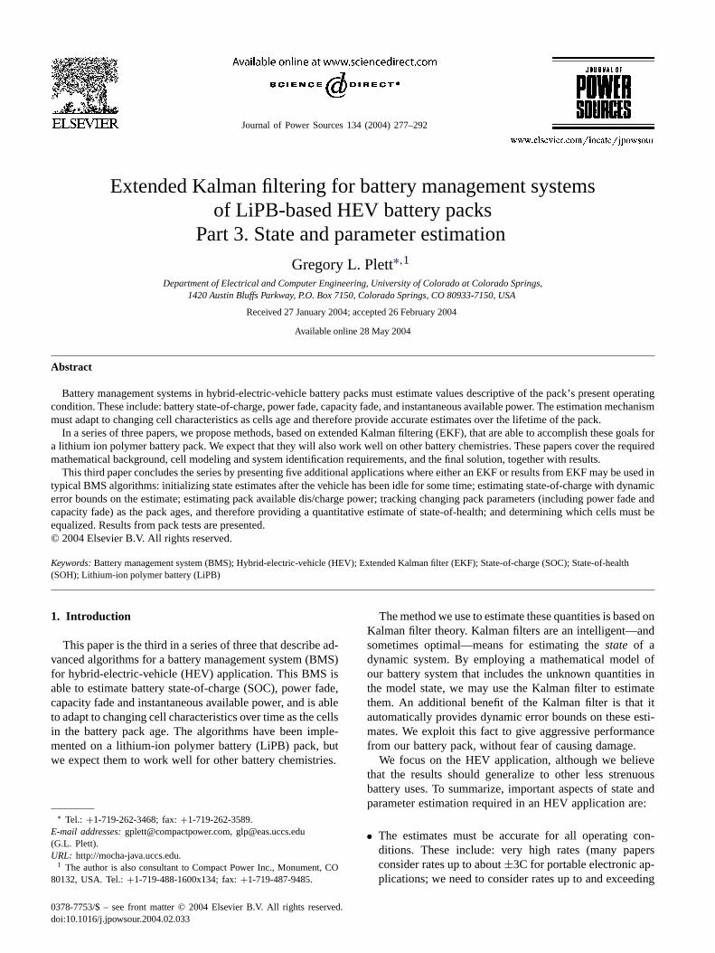
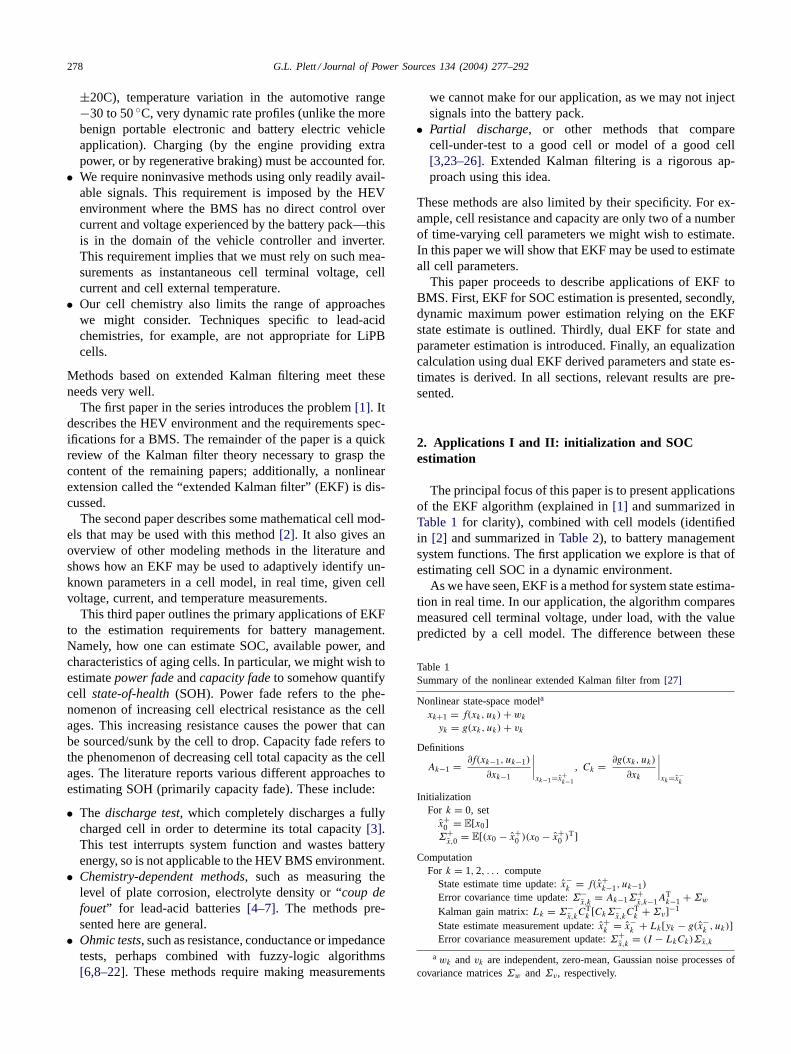
The principal focus of this paper is to present applicationsof the EKF algorithm (explained in[1] and summarized inTable 1for clarity), combined with cell models (identifiedin [2] and summarized inTable 2), to battery managementsystem functions. The first application we explore is that ofestimating cell SOC in a dynamic environment.

As we have seen, EKF is a method for system state estima-tion in real time. In our application, the algorithm comparesmeasured cell terminal voltage, under load, with the valuepredicted by a cell model. The difference between these

Table 1Summary of the nonlinear extended Kalman filter from[27]

Nonlinear state-space modela

xk+1 = f(xk, uk)+ wk

yk = g(xk, uk)+ vk

Definitions

Ak−1 = ∂f(xk−1, uk−1)

∂xk−1

∣∣∣∣xk−1=x+

k−1

, Ck = ∂g(xk, uk)

∂xk

∣∣∣∣xk=x−

k

InitializationFor k = 0, setx+

0 = E[x0]Σ+x,0 = E[(x0 − x+

0 )(x0 − x+0 )

T]

ComputationFor k = 1,2, . . . compute

State estimate time update:x−k = f(x+

k−1, uk−1)

Error covariance time update:Σ−x,k

= Ak−1Σ+x,k−1A

Tk−1 +Σw

Kalman gain matrix:Lk = Σ−x,kCTk [CkΣ

−x,kCTk +Σv]−1

State estimate measurement update:x+k = x−

k + Lk [yk − g(x−k , uk)]

Error covariance measurement update:Σ+x,k

= (I − LkCk)Σx,k

awk andvk are independent, zero-mean, Gaussian noise processes ofcovariance matricesΣw andΣv, respectively.

G.L. Plett / Journal of Power Sources 134 (2004) 277–292 279

Table 2Summary of cell models from[2]

Combined model: note thatK0 throughK4 are constants to fit the model

zk+1 = zk −(ηit

C

)ik

yk = K0 − Rik − K1

zk−K2zk +K3 ln(zk)+K4 ln(1 − zk)

Simple model: note that OCV(·) is open-circuit-voltage

zk+1 = zk −(ηit

C

)ik

yk = OCV(zk)− Rik

Zero-state hysteresis model: note thatM(·) is maximum hysteresis

zk+1 = zk −(ηit

C

)ik

yk = OCV(zk)− skM(zk)− Rik

Single-state hysteresis model: note thatF(ik) = exp

(−

∣∣∣∣ηiikγtC

∣∣∣∣)

, γ is hysteresis rate constant,M(·, ·) is maximum hysteresis

[hk+1

zk+1

]=

[F(ik) 0

0 1

] [hk

zk

]+

0 (1 − F(ik))

−ηit

C0

[

ik

M(z, z)

]

yk = OCV(zk)− Rik + hk

Enhanced self-correcting (ESC) model:α are filter-pole locationsfk+1

hk+1

zk+1

=

diag(α) 0 0

0 F(ik) 0

0 0 1

fk

hk

zk

+

1 0

0 (1 − F(ik))

−ηit

C0

[ik

M(z, z)

]

yk = OCV(zk)− Rik + hk + Gfk

zk is SOC,ηi the Coulombic efficiency,ik the current,yk the predicted cell voltage,t the sampling interval,C the nominal capacity,R the cell resistance.

quantities is used to adapt the state of the cell model so thatthe model output more closely matches the measured cellvoltage, and the model state more closely matches the realquantities it estimates. By enforcing that SOC be a memberof the model state, as is the case with all model structures inTable 2, we directly estimateboth SOC and the uncertainty(error bounds) of the estimate. Note that since we use EKFversus KF, we are able to use precise nonlinear cell modelsin our SOC estimator, improving the SOC estimation accu-racy.

Before presenting some results, we first discuss how thealgorithm’s state and uncertainties might be initialized whenthe vehicle is started. That is, how we might propagatezkandΣz,k across the interval between key-off and key-on. Forthis, we employ the SOC estimate andΣz values saved whenthe vehicle was previously turned off, the period of time thevehicle was off, and a very simple cell self-discharge model.Our empirical data indicates that SOC decays approximatelyexponentially due to self-discharge, allowing us to createa continuous-time state-space model for self-discharge. Letz(t) be the state-of-charge as a function of self-dischargetime. Then

z(t) = −φz(t)+ w(t)

y(t) = OCV(z(t))+ v(t),

whereφ is the rate of SOC decay,w is small andv dependson the period since key-off. We can form a discrete-time

version of this model. Lettoff be the period that the vehicleis off. Then,

zk+1 = e−φtoff zk + wk

yk = OCV(zk)+ vk.

Applying the EKF to this system estimates SOC andΣz.Filter states are initialized to zero withΣ

finitialized to small

values. The hysteresis state and covariance are unchangedby power-down.

In order to demonstrate the performance of EKF in esti-mating SOC with the various cell models, we need to firstdiscuss some cell tests. Data was gathered from a proto-type hand-made LiPB cell comprising a LiMn2O4 cathode,an artificial graphite anode, and designed for high-powerapplications, having a nominal capacity of 7.5 Ah and anominal voltage of 3.8 V. For the tests, we used a Tenneythermal chamber set at 25C and an Arbin BT2000 cellcycler. Each channel of the Arbin was capable of 20 A cur-rent, and 10 channels were connected in parallel to achievecurrents of up to 200 A. The cycler’s voltage measurementaccuracy was±5 mV and its current measurement accuracywas±200 mA. Two different cell tests were performed:

• Pulsed-current test: The first test comprised a sequenceof discharge pulses and rests followed by a sequence ofcharge pulses and rests. This test was designed to ex-plore the cell response to very high and very low currents


0 10 20 30 40 50 60 70

0

10

20

30

40

50

60

70

80

90

100

SOC and current as a function of time during discharge

Time (min.)

SO

C (

perc

ent)

0

20

40

60

80

100

120

140

160

180

200

Cur

rent

(A

)

SOCCurrent

10 20 30 40 50 60 70 80 90

0

10

20

30

40

50

60

70

80

90

100

SOC and current as a function of time during charge

Time (min.)

SO

C (

perc

ent)

200

180

160

140

120

100

80

60

40

20

0

Cur

rent

(A

)

SOCCurrent

(a) (b)

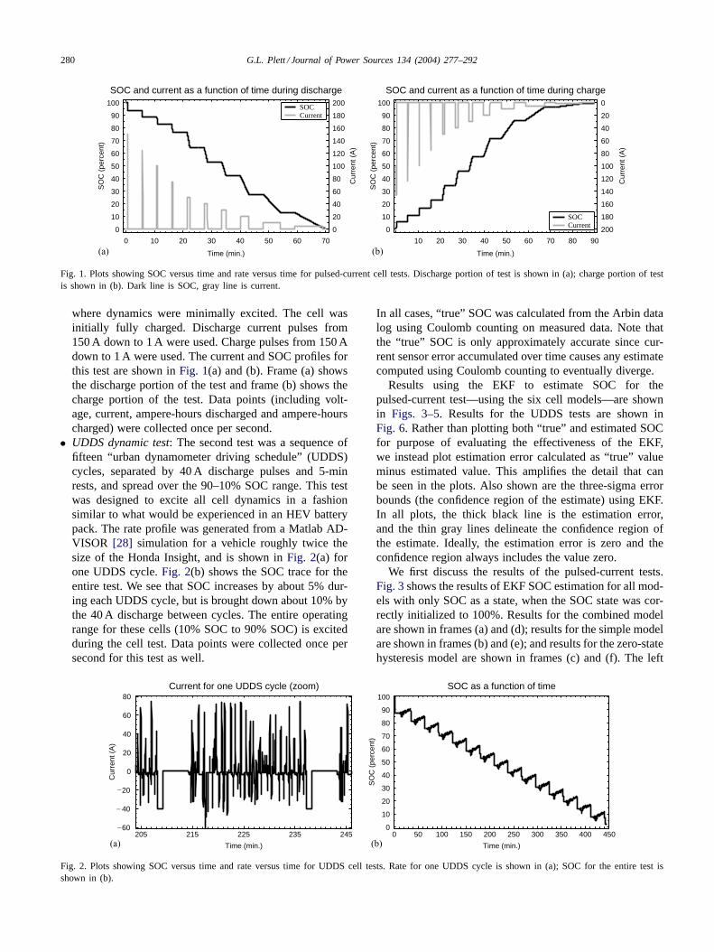
Fig. 1. Plots showing SOC versus time and rate versus time for pulsed-current cell tests. Discharge portion of test is shown in (a); charge portion of testis shown in (b). Dark line is SOC, gray line is current.

where dynamics were minimally excited. The cell wasinitially fully charged. Discharge current pulses from150 A down to 1 A were used. Charge pulses from 150 Adown to 1 A were used. The current and SOC profiles forthis test are shown in Fig. 1(a) and (b). Frame (a) showsthe discharge portion of the test and frame (b) shows thecharge portion of the test. Data points (including volt-age, current, ampere-hours discharged and ampere-hourscharged) were collected once per second.

• UDDS dynamic test: The second test was a sequence offifteen “urban dynamometer driving schedule” (UDDS)cycles, separated by 40 A discharge pulses and 5-minrests, and spread over the 90–10% SOC range. This testwas designed to excite all cell dynamics in a fashionsimilar to what would be experienced in an HEV batterypack. The rate profile was generated from a Matlab AD-VISOR [28] simulation for a vehicle roughly twice thesize of the Honda Insight, and is shown in Fig. 2(a) forone UDDS cycle. Fig. 2(b) shows the SOC trace for theentire test. We see that SOC increases by about 5% dur-ing each UDDS cycle, but is brought down about 10% bythe 40 A discharge between cycles. The entire operatingrange for these cells (10% SOC to 90% SOC) is excitedduring the cell test. Data points were collected once persecond for this test as well.

205 215 225 235 24560

40

20

0

20

40

60

80Current for one UDDS cycle (zoom)

Time (min.)

Cur

rent

(A

)

0 50 100 150 200 250 300 350 400 4500

10

20

30

40

50

60

70

80

90

100SOC as a function of time

Time (min.)

SO

C (

perc

ent)

_

_

_

(a) (b)

Fig. 2. Plots showing SOC versus time and rate versus time for UDDS cell tests. Rate for one UDDS cycle is shown in (a); SOC for the entire test isshown in (b).

In all cases, “ true” SOC was calculated from the Arbin datalog using Coulomb counting on measured data. Note thatthe “ true” SOC is only approximately accurate since cur-rent sensor error accumulated over time causes any estimatecomputed using Coulomb counting to eventually diverge.

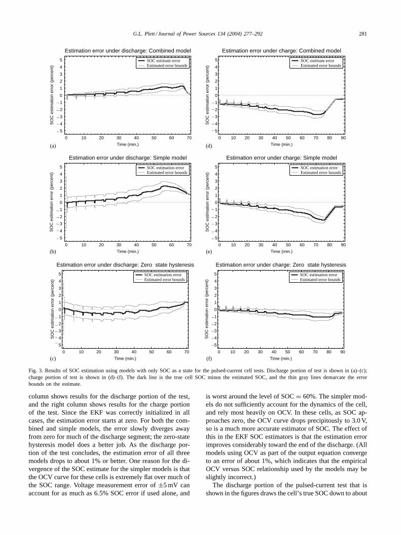
Results using the EKF to estimate SOC for thepulsed-current test—using the six cell models—are shownin Figs. 3–5. Results for the UDDS tests are shown inFig. 6. Rather than plotting both “ true” and estimated SOCfor purpose of evaluating the effectiveness of the EKF,we instead plot estimation error calculated as “ true” valueminus estimated value. This amplifies the detail that canbe seen in the plots. Also shown are the three-sigma errorbounds (the confidence region of the estimate) using EKF.In all plots, the thick black line is the estimation error,and the thin gray lines delineate the confidence region ofthe estimate. Ideally, the estimation error is zero and theconfidence region always includes the value zero.

We first discuss the results of the pulsed-current tests.Fig. 3 shows the results of EKF SOC estimation for all mod-els with only SOC as a state, when the SOC state was cor-rectly initialized to 100%. Results for the combined modelare shown in frames (a) and (d); results for the simple modelare shown in frames (b) and (e); and results for the zero-statehysteresis model are shown in frames (c) and (f). The left


0 10 20 30 40 50 60 70

5

4

3

2

1

0

1

2

3

4

5

Estimation error under discharge: Combined model

Time (min.)

SO

C e

stim

atio

n er

ror

(per

cent

)

SOC estimate errorEstimated error bounds

0 10 20 30 40 50 60 70 80 90

5

4

3

2

1

0

1

2

3

4

5

Estimation error under charge: Combined model

Time (min.)

SO

C e

stim

atio

n er

ror

(per

cent

)


(a) (d)

0 10 20 30 40 50 60 70

5

4

3

2

1

0

1

2

3

4

5

Estimation error under discharge: Simple model

Time (min.)

SO

C e

stim

atio

n er

ror

(per

cent

)

SOC estimation errorEstimated error bounds

0 10 20 30 40 50 60 70 80 90

5

4

3

2

1

0

1

2

3

4

5

Estimation error under charge: Simple model

Time (min.)

SO

C e

stim

atio

n er

ror

(per

cent

)


(b) (e)

0 10 20 30 40 50 60 70

5

4

3

2

1

0

1

2

3

4

5

Estimation error under discharge: Zero state hysteresis

Time (min.)

SO

C e

stim

atio

n er

ror

(per

cent

)


0 10 20 30 40 50 60 70 80 90

5

4

3

2

1

0

1

2

3

4

5

Estimation error under charge: Zero state hysteresis

Time (min.)

SO

C e

stim

atio

n er

ror

(per

cent

)


(c) (f)

_

_

_ _

_

_

_

_

__

_

_

_

_

_ _

_

_

_

_

_

_

_

_

_

_

_

_

__

Fig. 3. Results of SOC estimation using models with only SOC as a state for the pulsed-current cell tests. Discharge portion of test is shown in (a)–(c);charge portion of test is shown in (d)–(f). The dark line is the true cell SOC minus the estimated SOC, and the thin gray lines demarcate the errorbounds on the estimate.

column shows results for the discharge portion of the test,and the right column shows results for the charge portionof the test. Since the EKF was correctly initialized in allcases, the estimation error starts at zero. For both the com-bined and simple models, the error slowly diverges awayfrom zero for much of the discharge segment; the zero-statehysteresis model does a better job. As the discharge por-tion of the test concludes, the estimation error of all threemodels drops to about 1% or better. One reason for the di-vergence of the SOC estimate for the simpler models is thatthe OCV curve for these cells is extremely flat over much ofthe SOC range. Voltage measurement error of ±5 mV canaccount for as much as 6.5% SOC error if used alone, and

is worst around the level of SOC = 60%. The simpler mod-els do not sufficiently account for the dynamics of the cell,and rely most heavily on OCV. In these cells, as SOC ap-proaches zero, the OCV curve drops precipitously to 3.0 V,so is a much more accurate estimator of SOC. The effect ofthis in the EKF SOC estimators is that the estimation errorimproves considerably toward the end of the discharge. (Allmodels using OCV as part of the output equation convergeto an error of about 1%, which indicates that the empiricalOCV versus SOC relationship used by the models may beslightly incorrect.)

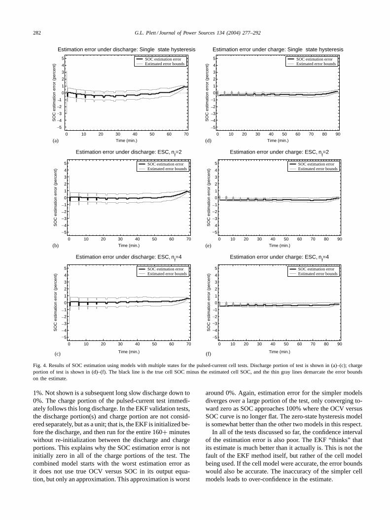
The discharge portion of the pulsed-current test that isshown in the figures draws the cell’s true SOC down to about


0 10 20 30 40 50 60 70

5

4

3

2

1

0

1

2

3

4

5

Estimation error under discharge: Single state hysteresis

Time (min.)

SO

C e

stim

atio

n er

ror

(per

cent

)SOC estimation errorEstimated error bounds

0 10 20 30 40 50 60 70 80 90

5

4

3

2

1

0

1

2

3

4

5

Estimation error under charge: Single state hysteresis

Time (min.)

SO

C e

stim

atio

n er

ror

(per

cent

)


(a) (d)

0 10 20 30 40 50 60 70

5

4

3

2

1

0

1

2

3

4

5

Estimation error under discharge: ESC, nf=2

Time (min.)

SO

C e

stim

atio

n er

ror

(per

cent

)


0 10 20 30 40 50 60 70 80 90

5

4

3

2

1

0

1

2

3

4

5

Estimation error under charge: ESC, nf=2

Time (min.)

SO

C e

stim

atio

n er

ror

(per

cent

)


(b) (e)

0 10 20 30 40 50 60 70

5

4

3

2

1

0

1

2

3

4

5


Time (min.)

SO

C e

stim

atio

n er

ror

(per

cent

)


0 10 20 30 40 50 60 70 80 90

5

4

3

2

1

0

1

2

3

4

5

Estimation error under charge: ESC, nf=4

Time (min.)

SO

C e

stim

atio

n er

ror

(per

cent

)


(c) (f)

_

_

_

_

_ _

_

_

_

_

_

_

_

_

_

_

_

_

_

_ _

_

_

_

_

_

_

_

_

Fig. 4. Results of SOC estimation using models with multiple states for the pulsed-current cell tests. Discharge portion of test is shown in (a)–(c); chargeportion of test is shown in (d)–(f). The black line is the true cell SOC minus the estimated cell SOC, and the thin gray lines demarcate the error boundson the estimate.

1%. Not shown is a subsequent long slow discharge down to0%. The charge portion of the pulsed-current test immedi-ately follows this long discharge. In the EKF validation tests,the discharge portion(s) and charge portion are not consid-ered separately, but as a unit; that is, the EKF is initialized be-fore the discharge, and then run for the entire 160+ minuteswithout re-initialization between the discharge and chargeportions. This explains why the SOC estimation error is notinitially zero in all of the charge portions of the test. Thecombined model starts with the worst estimation error asit does not use true OCV versus SOC in its output equa-tion, but only an approximation. This approximation is worst

around 0%. Again, estimation error for the simpler modelsdiverges over a large portion of the test, only converging to-ward zero as SOC approaches 100% where the OCV versusSOC curve is no longer flat. The zero-state hysteresis modelis somewhat better than the other two models in this respect.

In all of the tests discussed so far, the confidence intervalof the estimation error is also poor. The EKF “ thinks” thatits estimate is much better than it actually is. This is not thefault of the EKF method itself, but rather of the cell modelbeing used. If the cell model were accurate, the error boundswould also be accurate. The inaccuracy of the simpler cellmodels leads to over-confidence in the estimate.


0 10 20 30 40 50 60 70

10

8

6

4

2

0

2

4

6

8

10

Estimation error under discharge: Combined model

Time (min.)

SO

C e

stim

atio

n er

ror

(per

cent

)


0 10 20 30 40 50 60 70

10

8

6

4

2

0

2

4

6

8

10

Estimation error under discharge: Simple model

Time (min.)

SO

C e

stim

atio

n er

ror

(per

cent

)


(a) (d)

0 10 20 30 40 50 60 70

10

8

6

4

2

0

2

4

6

8

10

Estimation error under discharge: Zero state hysteresis

Time (min.)

SO

C e

stim

atio

n er

ror

(per

cent

)


0 10 20 30 40 50 60 70

10

8

6

4

2

0

2

4

6

8

10

Estimation error under discharge: Single state hysteresis

Time (min.)

SO

C e

stim

atio

n er

ror

(per

cent

)


(b) (e)

0 10 20 30 40 50 60 70

10

8

6

4

2

0

2

4

6

8

10


Time (min.)

SO

C e

stim

atio

n er

ror

(per

cent

)


0 10 20 30 40 50 60 70

10

8

6

4

2

0

2

4

6

8

10


Time (min.)

SO

C e

stim

atio

n er

ror

(per

cent

)


(c) (f)

_

_

_

_

_

_

_

_

_

_

_

_

_

_

_

_

_

_

_

_

_

_

_

_

_

_

_

_

_

_

Fig. 5. Results of SOC estimation where the initial estimator state was set to 80% while the true initial state was 100%. The dark line is the true cellSOC minus the estimated SOC, and the thin gray lines demarcate the error bounds on the estimate.

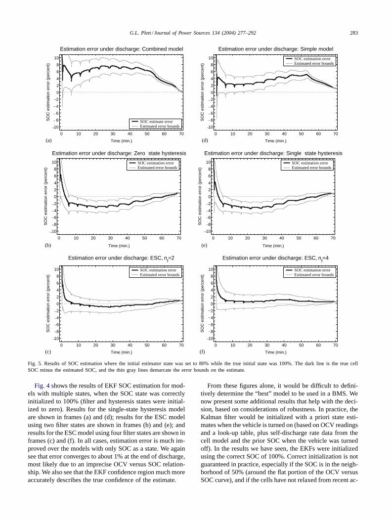
Fig. 4 shows the results of EKF SOC estimation for mod-els with multiple states, when the SOC state was correctlyinitialized to 100% (filter and hysteresis states were initial-ized to zero). Results for the single-state hysteresis modelare shown in frames (a) and (d); results for the ESC modelusing two filter states are shown in frames (b) and (e); andresults for the ESC model using four filter states are shown inframes (c) and (f). In all cases, estimation error is much im-proved over the models with only SOC as a state. We againsee that error converges to about 1% at the end of discharge,most likely due to an imprecise OCV versus SOC relation-ship. We also see that the EKF confidence region much moreaccurately describes the true confidence of the estimate.

From these figures alone, it would be difficult to defini-tively determine the “best” model to be used in a BMS. Wenow present some additional results that help with the deci-sion, based on considerations of robustness. In practice, theKalman filter would be initialized with a priori state esti-mates when the vehicle is turned on (based on OCV readingsand a look-up table, plus self-discharge rate data from thecell model and the prior SOC when the vehicle was turnedoff). In the results we have seen, the EKFs were initializedusing the correct SOC of 100%. Correct initialization is notguaranteed in practice, especially if the SOC is in the neigh-borhood of 50% (around the flat portion of the OCV versusSOC curve), and if the cells have not relaxed from recent ac-


0 60 120 180 240 300 360 420 4804

3

2

1

0

1

2

3

4

5

6

Estimation error: ESC, nf=4

Time (min.)

SO

C e

stim

atio

n er

ror

(per

cent

)SOC estimation errorEstimated error bounds

0 1 2 3 4 5 6 4 2

02Zoom of first minutes

0 60 120 180 240 300 360 420 480 6

4

2

0

2

4

6

8

10

12

14

16

Estimation error: ESC, nf=4

Time (min.)

SO

C e

stim

atio

n er

ror

(per

cent

)


0 1 2 3 4 5 10

0

10

20Zoom of first minutes

(a) (b)

_

_

_

_

_

_

__

_

_

_

_

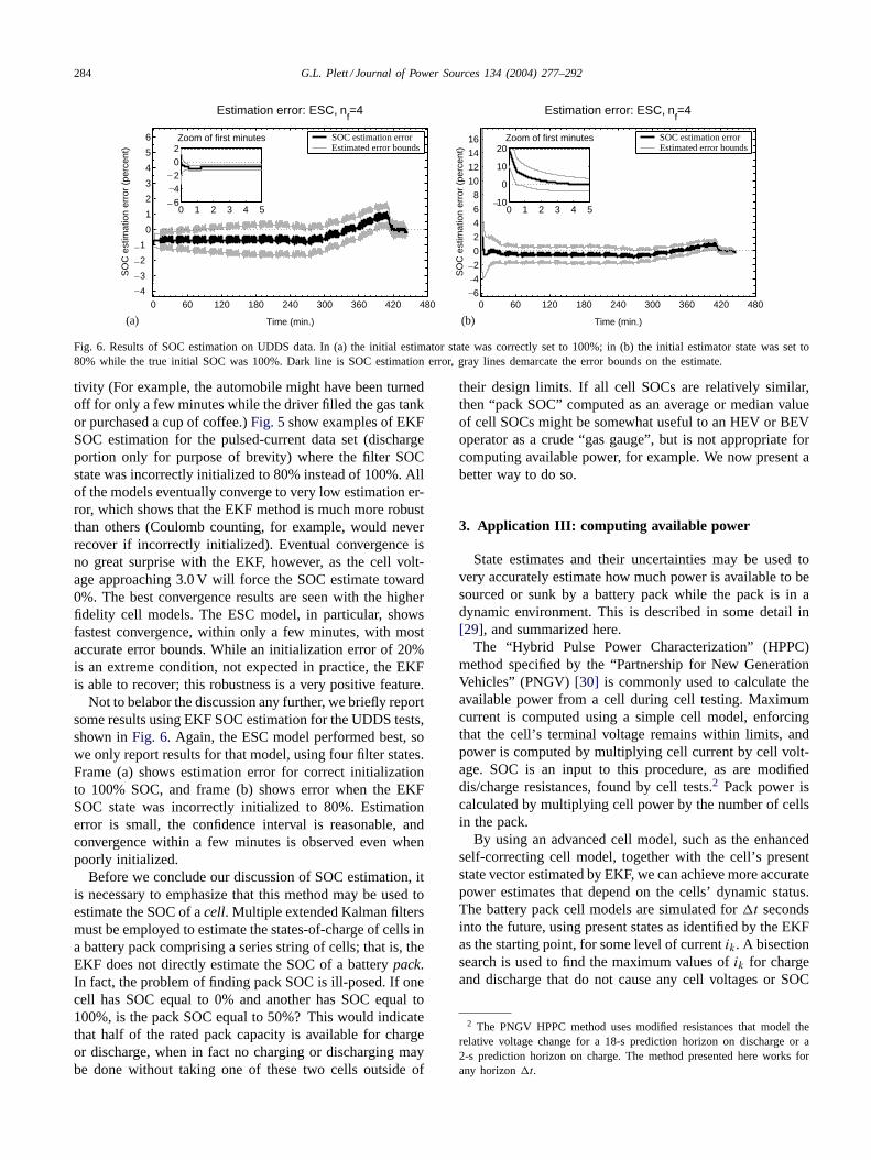
Fig. 6. Results of SOC estimation on UDDS data. In (a) the initial estimator state was correctly set to 100%; in (b) the initial estimator state was set to80% while the true initial SOC was 100%. Dark line is SOC estimation error, gray lines demarcate the error bounds on the estimate.

tivity (For example, the automobile might have been turnedoff for only a few minutes while the driver filled the gas tankor purchased a cup of coffee.) Fig. 5 show examples of EKFSOC estimation for the pulsed-current data set (dischargeportion only for purpose of brevity) where the filter SOCstate was incorrectly initialized to 80% instead of 100%. Allof the models eventually converge to very low estimation er-ror, which shows that the EKF method is much more robustthan others (Coulomb counting, for example, would neverrecover if incorrectly initialized). Eventual convergence isno great surprise with the EKF, however, as the cell volt-age approaching 3.0 V will force the SOC estimate toward0%. The best convergence results are seen with the higherfidelity cell models. The ESC model, in particular, showsfastest convergence, within only a few minutes, with mostaccurate error bounds. While an initialization error of 20%is an extreme condition, not expected in practice, the EKFis able to recover; this robustness is a very positive feature.

Not to belabor the discussion any further, we briefly reportsome results using EKF SOC estimation for the UDDS tests,shown in Fig. 6. Again, the ESC model performed best, sowe only report results for that model, using four filter states.Frame (a) shows estimation error for correct initializationto 100% SOC, and frame (b) shows error when the EKFSOC state was incorrectly initialized to 80%. Estimationerror is small, the confidence interval is reasonable, andconvergence within a few minutes is observed even whenpoorly initialized.

Before we conclude our discussion of SOC estimation, itis necessary to emphasize that this method may be used toestimate the SOC of a cell. Multiple extended Kalman filtersmust be employed to estimate the states-of-charge of cells ina battery pack comprising a series string of cells; that is, theEKF does not directly estimate the SOC of a battery pack.In fact, the problem of finding pack SOC is ill-posed. If onecell has SOC equal to 0% and another has SOC equal to100%, is the pack SOC equal to 50%? This would indicatethat half of the rated pack capacity is available for chargeor discharge, when in fact no charging or discharging maybe done without taking one of these two cells outside of

their design limits. If all cell SOCs are relatively similar,then “pack SOC” computed as an average or median valueof cell SOCs might be somewhat useful to an HEV or BEVoperator as a crude “gas gauge” , but is not appropriate forcomputing available power, for example. We now present abetter way to do so.

3. Application III: computing available power

State estimates and their uncertainties may be used tovery accurately estimate how much power is available to besourced or sunk by a battery pack while the pack is in adynamic environment. This is described in some detail in[29], and summarized here.

The “Hybrid Pulse Power Characterization” (HPPC)method specified by the “Partnership for New GenerationVehicles” (PNGV) [30] is commonly used to calculate theavailable power from a cell during cell testing. Maximumcurrent is computed using a simple cell model, enforcingthat the cell’s terminal voltage remains within limits, andpower is computed by multiplying cell current by cell volt-age. SOC is an input to this procedure, as are modifieddis/charge resistances, found by cell tests.2 Pack power iscalculated by multiplying cell power by the number of cellsin the pack.

By using an advanced cell model, such as the enhancedself-correcting cell model, together with the cell’s presentstate vector estimated by EKF, we can achieve more accuratepower estimates that depend on the cells’ dynamic status.The battery pack cell models are simulated for t secondsinto the future, using present states as identified by the EKFas the starting point, for some level of current ik. A bisectionsearch is used to find the maximum values of ik for chargeand discharge that do not cause any cell voltages or SOC

2 The PNGV HPPC method uses modified resistances that model therelative voltage change for a 18-s prediction horizon on discharge or a2-s prediction horizon on charge. The method presented here works forany horizon t.


0 10 20 30 40 50 60 70

0

5

10

15

20

25

Available power under discharge

Time (min.)

Pow

er (

kW)

EKF charge powerHPPC charge powerEKF discharge powerHPPC discharge power

0 10 20 30 40 50 60 70

0

5

10

15

20

25

Available power under charge

Time (min.)

Pow

er (

kW)

EKF charge powerHPPC charge powerEKF discharge powerHPPC discharge power

(a) (b)

Fig. 7. Results of power estimation on pulsed-current data. Frame (a) shows the power estimates for the discharge portion of the test; Frame (b) showsthe estimates for the charge portion of the tests.

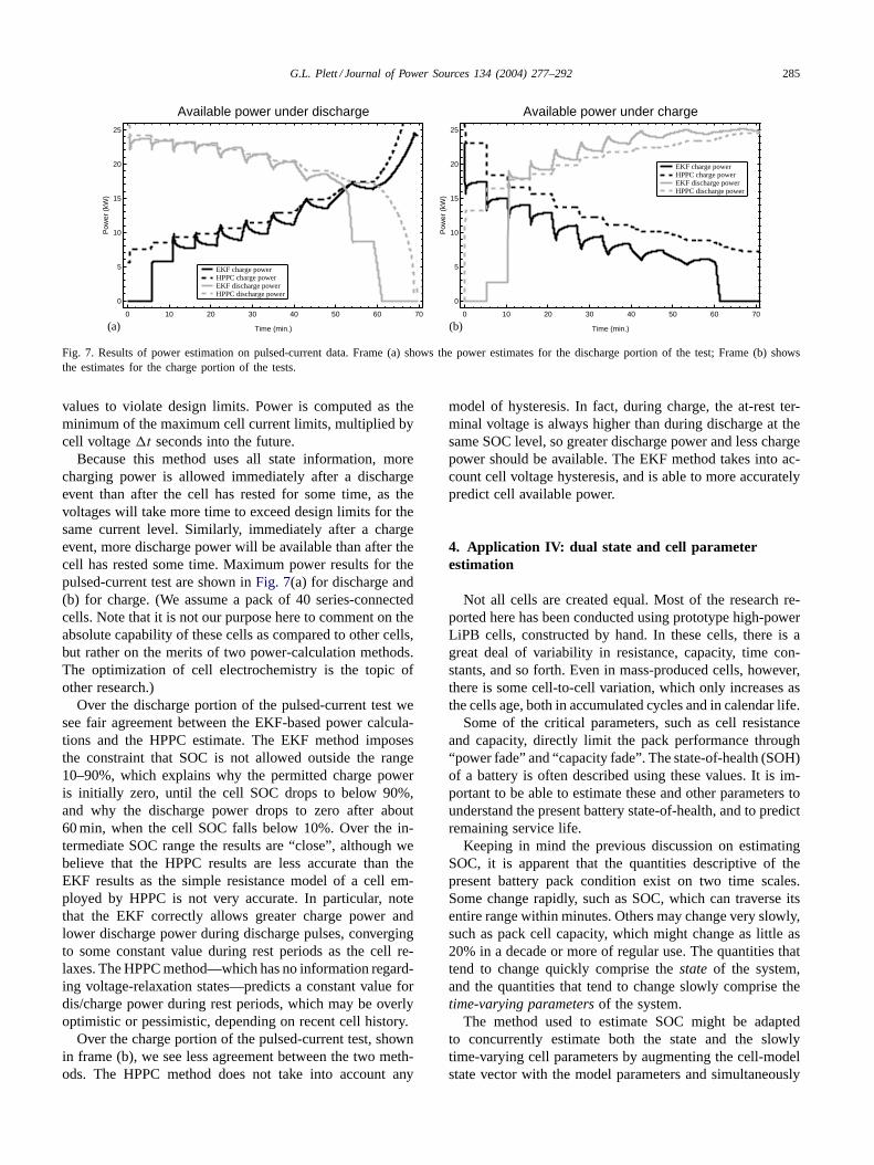
values to violate design limits. Power is computed as theminimum of the maximum cell current limits, multiplied bycell voltage t seconds into the future.

Because this method uses all state information, morecharging power is allowed immediately after a dischargeevent than after the cell has rested for some time, as thevoltages will take more time to exceed design limits for thesame current level. Similarly, immediately after a chargeevent, more discharge power will be available than after thecell has rested some time. Maximum power results for thepulsed-current test are shown in Fig. 7(a) for discharge and(b) for charge. (We assume a pack of 40 series-connectedcells. Note that it is not our purpose here to comment on theabsolute capability of these cells as compared to other cells,but rather on the merits of two power-calculation methods.The optimization of cell electrochemistry is the topic ofother research.)

Over the discharge portion of the pulsed-current test wesee fair agreement between the EKF-based power calcula-tions and the HPPC estimate. The EKF method imposesthe constraint that SOC is not allowed outside the range10–90%, which explains why the permitted charge poweris initially zero, until the cell SOC drops to below 90%,and why the discharge power drops to zero after about60 min, when the cell SOC falls below 10%. Over the in-termediate SOC range the results are “close” , although webelieve that the HPPC results are less accurate than theEKF results as the simple resistance model of a cell em-ployed by HPPC is not very accurate. In particular, notethat the EKF correctly allows greater charge power andlower discharge power during discharge pulses, convergingto some constant value during rest periods as the cell re-laxes. The HPPC method—which has no information regard-ing voltage-relaxation states—predicts a constant value fordis/charge power during rest periods, which may be overlyoptimistic or pessimistic, depending on recent cell history.

Over the charge portion of the pulsed-current test, shownin frame (b), we see less agreement between the two meth-ods. The HPPC method does not take into account any

model of hysteresis. In fact, during charge, the at-rest ter-minal voltage is always higher than during discharge at thesame SOC level, so greater discharge power and less chargepower should be available. The EKF method takes into ac-count cell voltage hysteresis, and is able to more accuratelypredict cell available power.

4. Application IV: dual state and cell parameterestimation

Not all cells are created equal. Most of the research re-ported here has been conducted using prototype high-powerLiPB cells, constructed by hand. In these cells, there is agreat deal of variability in resistance, capacity, time con-stants, and so forth. Even in mass-produced cells, however,there is some cell-to-cell variation, which only increases asthe cells age, both in accumulated cycles and in calendar life.

Some of the critical parameters, such as cell resistanceand capacity, directly limit the pack performance through“power fade” and “capacity fade” . The state-of-health (SOH)of a battery is often described using these values. It is im-portant to be able to estimate these and other parameters tounderstand the present battery state-of-health, and to predictremaining service life.

Keeping in mind the previous discussion on estimatingSOC, it is apparent that the quantities descriptive of thepresent battery pack condition exist on two time scales.Some change rapidly, such as SOC, which can traverse itsentire range within minutes. Others may change very slowly,such as pack cell capacity, which might change as little as20% in a decade or more of regular use. The quantities thattend to change quickly comprise the state of the system,and the quantities that tend to change slowly comprise thetime-varying parameters of the system.

The method used to estimate SOC might be adaptedto concurrently estimate both the state and the slowlytime-varying cell parameters by augmenting the cell-modelstate vector with the model parameters and simultaneously


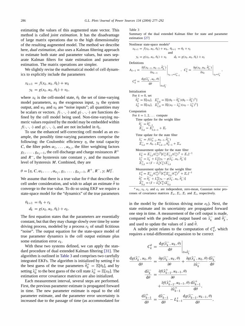
estimating the values of this augmented state vector. Thismethod is called joint estimation. It has the disadvantageof large matrix operations due to the high dimensionalityof the resulting augmented model. The method we describehere, dual estimation, also uses a Kalman filtering approachto estimate both state and parameter values, but uses sep-arate Kalman filters for state estimation and parameterestimation. The matrix operations are simpler.

We slightly revise the mathematical model of cell dynam-ics to explicitly include the parameters

xk+1 = f(xk, uk, θk)+ wk

yk = g(xk, uk, θk)+ vk,

where xk is the cell-model state, θk the set of time-varyingmodel parameters, uk the exogenous input, yk the systemoutput, and wk and vk are “noise inputs” ; all quantities maybe scalars or vectors. f(·, ·, ·) and g(·, ·, ·) are functions de-fined by the cell model being used. Non-time-varying nu-meric values required by the model may be embedded withinf(·, ·, ·) and g(·, ·, ·), and are not included in θk.

To use the enhanced self-correcting cell model as an ex-ample, the possibly time-varying parameters comprise thefollowing: the Coulombic efficiency η, the total capacityC, the filter poles α1, . . . , αnf , the filter weighting factorsg1, . . . , gnf−1, the cell discharge and charge resistances R+

and R−, the hysteresis rate constant γ , and the maximumlevel of hysteresis M. Combined, they are

θ = [η,C, α1, . . . , αnf , g1, . . . , gnf−1, R+, R−, γ,M]′.

We assume that there is a true value for θ that describes thecell under consideration, and wish to adapt an estimate θ toconverge to the true value. To do so using EKF we require astate-space model for the “dynamics” of the true parameters

θk+1 = θk + rk

dk = g(xk, uk, θk)+ ek.

The first equation states that the parameters are essentiallyconstant, but that they may change slowly over time by somedriving process, modeled by a process rk of small fictitious“noise” . The output equation for the state-space model oftrue parameter dynamics is the cell output estimate plussome estimation error ek.

With these two systems defined, we can apply the stan-dard procedure of dual extended Kalman filtering [31]. Thealgorithm is outlined in Table 3 and comprises two carefullyintegrated EKFs. The algorithm is initialized by setting θ tothe best guess of the true parameters θ+

0 = E[θ0], and bysetting x+

0 to the best guess of the cell state x+0 = E[x0]. The

estimation error covariance matrices are also initialized.Each measurement interval, several steps are performed.

First, the previous parameter estimate is propagated forwardin time. The new parameter estimate is equal to the oldparameter estimate, and the parameter error uncertainty isincreased due to the passage of time (as accommodated for

Table 3Summary of the dual extended Kalman filter for state and parameterestimation [27]

Nonlinear state-space modelsa

xk+1 = f(xk, uk, θk)+ wk , θk+1 = θk + rkand

yk = g(xk, uk, θk)+ vk dk = g(xk, uk, θk)+ ek

Definitions

Ak−1 = ∂f(xk−1, uk−1, θ−k )

∂xk−1

∣∣∣∣∣xk−1=x+

k−1

, Cxk = ∂g(xk, uk, θ

−k )

∂xk

∣∣∣∣∣xk=x−

k

,

Cθk = dg(x−

k , uk, θ)

dθ

∣∣∣∣∣θ=θ−

k

InitializationFor k = 0, setθ+

0 = E[x0], Σ+θ,0

= E[(θ0 − θ+0 )(θ0 − θ+

0 )T]

x+0 = E[x0], Σ+

x,0 = E[(x0 − x+0 )(x0 − x+

0 )T]

ComputationFor k = 1, 2, . . . compute

Time update for the weight filterθ−k = θ+

k−1Σ−θ,k

= Σ+θ,k−1

+Σr

Time update for the state filterx−k = f(x+

k−1, uk−1, θ−k )

Σ−x,k

= Ak−1Σ+x,k−1A

Tk−1 +Σw

Measurement update for the state filterLxk = Σ−

x,k(Cx

k )T[Cx

kΣ−x,k(Cx

k )T +Σv]−1

x+k = x−

k + Lxk[yk − g(x−

k , uk, θ−k )]

Σ+x,k

= (I − LxkC

xk)Σ

−x,k

Measurement update for the weight filterLθk = Σ−

θ,k(Cθ

k)T[Cθ

kΣ−θ,k(Cθ

k)T +Σe]−1

θ+k = θ−

k + Lθk[yk − g(x−

k , uk, θ−k )]

Σ+θ,k

= (I − LθkC

θk)Σ

−θ,k

a wk, vk, rk and ek are independent, zero-mean, Gaussian noise pro-cesses of covariance matrices Σw,Σv,Σr and Σe, respectively.

in the model by the fictitious driving noise ek). Next, thestate estimate and its uncertainty are propagated forwardone step in time. A measurement of the cell output is made,compared with the predicted output based on x−

k and θ−k ,

and used to update the values of x and θ.A subtle point relates to the computation of Cθ

k , whichrequires a total-differential expansion to be correct

Cθk = dg(x−

k , uk, θ)

dθ

∣∣∣∣∣θ=θ−

k

dg(x−k , uk, θ)

dθ= ∂g(x−

k , uk, θ)

∂θ+ ∂g(x−

k , uk, θ)

∂x−k

dx−k

dθ

dx−k

dθ= ∂f(x+

k−1, uk−1, θ)

∂θ

+∂f(x+k−1, uk−1, θ)

∂x+k−1

dx+k−1

dθ,

dx+k−1

dθ= dx−

k−1

dθ− Lxk−1

dg(x−k−1, uk−1, θ)

dθ,


Time UpdateEKFx

Time UpdateEKEq

MeasurementUpdate EKFx

MeasurementUpdate EKF

x+k−1

qΣ

Σ

ΣΣ

qq

q

q

q+k−1

x−k

ˆ−k

x+k

+k

−x , k

−˜ k

+x ,

,

k−1

+˜ k−1

yk

uk−1

uk

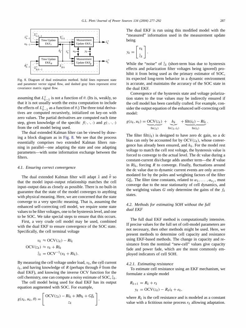
Fig. 8. Diagram of dual estimation method. Solid lines represent stateand parameter vector signal flow, and dashed gray lines represent errorcovariance matrix signal flow.

assuming that Lxk−1 is not a function of θ. (Its is, weakly, sothat it is not usually worth the extra computation to includethe effects of Lxk−1 as a function of θ.) The three total deriva-tives are computed recursively, initialized on key-on withzero values. The partial derivatives are computed each timestep, given knowledge of the specific f(·, ·, ·) and g(·, ·, ·)from the cell model being used.

The dual extended Kalman filter can be viewed by draw-ing a block diagram as in Fig. 8. We see that the processessentially comprises two extended Kalman filters run-ning in parallel—one adapting the state and one adaptingparameters—with some information exchange between thefilters.

4.1. Ensuring correct convergence

The dual extended Kalman filter will adapt x and θ sothat the model input–output relationship matches the cellinput–output data as closely as possible. There is no built-inguarantee that the state of the model converges to anythingwith physical meaning. Here, we are concerned that the stateconverge to a very specific meaning. That is, assuming theenhanced self-correcting cell model, we require some statevalues to be filter voltages, one to be hysteresis level, and oneto be SOC. We take special steps to ensure that this occurs.

First, a very crude cell model may be used, combinedwith the dual EKF to ensure convergence of the SOC state.Specifically, the cell terminal voltage

vk ≈ OCV(zk)− Rik

OCV(zk) ≈ vk + Rik

zk = OCV−1(vk + Rik).

By measuring the cell voltage under load, vk, the cell currentik, and having knowledge of R (perhaps through θ from thedual EKF), and knowing the inverse OCV function for thecell chemistry, one can compute a noisy estimate of SOC, zk.

The cell model being used for dual EKF has its outputequation augmented with SOC. For example,

g(xk, uk, θ) =[

OCV(zk)− Rik + Mhk + Gfkzk

].

The dual EKF is run using this modified model with the“measured” information used in the measurement updatebeing

yk =[vk

zk

].

While the “noise” of zk (short-term bias due to hysteresiseffects and polarization filter voltages being ignored) pro-hibit it from being used as the primary estimator of SOC,its expected long-term behavior in a dynamic environmentis accurate, and maintains the accuracy of the SOC state inthe dual EKF.

Convergence of the hysteresis state and voltage polariza-tion states to the true values may be indirectly ensured ifthe cell model has been carefully crafted. For example, con-sider the output equation of the enhanced self-correcting cellmodel:

g(xk, uk) = OCV(zk)︸︷︷︸fn(zk)

+ hk︸︷︷︸fn(zk,ik)

+ filt(ik)− Rik︸︷︷︸fn(ik)

.

The filter filt(ik) is designed to have zero dc gain, so a dcbias can only be accounted for by OCV(zk), whose conver-gence has already been ensured, and hk. For the model restvoltage to match the cell rest voltage, the hysteresis value isforced to converge to the actual level. The dc value during aconstant-current dis/charge adds another term—the R valuein Rik, forcing R to converge. Finally, fluctuations aroundthe dc value due to dynamic current events are only accom-modated for by the poles and weighting factors of the filterGfk. The filter time constants, related to α1, . . . , αnf , mustconverge due to the near stationarity of cell dynamics, andthe weighting values G only determine the gains of the fkstates.

4.2. Methods for estimating SOH without the fulldual EKF

The full dual EKF method is computationally intensive.If precise values for the full set of cell-model parameters arenot necessary, then other methods might be used. Here, wepresent methods to determine cell capacity and resistanceusing EKF-based methods. The change in capacity and re-sistance from the nominal “new-cell” values give capacityfade and power fade, which are the most commonly em-ployed indicators of cell SOH.

4.2.1. Estimating resistanceTo estimate cell resistance using an EKF mechanism, we

formulate a simple model

Rk+1 = Rk + rk

yk = OCV(zk)− Rkik + ek,

where Rk is the cell resistance and is modeled as a constantvalue with a fictitious noise process rk allowing adaptation.


yk is a crude estimate of the cell’s voltage, ik is the cell cur-rent, and ek models estimation error. If we use an estimate ofzk from the state EKF, or from some other source, we simplyapply an EKF to this model to estimate cell resistance. Inthe standard EKF, we compute the model’s prediction of ykwith the true measured cell voltage, and use the differenceto adapt Rk.

Note that the above model may be extended to handledifferent values of resistance on charge and discharge, dif-ferent values of resistance at different SOCs, and differentvalues of resistance at different temperatures, for example.The scalar Rk would be changed into a vector comprisingall of the resistance values being modified, and the appro-priate element from the vector would be used each time stepof the EKF during the calculations.

4.2.2. Estimating capacityTo estimate cell capacity using an EKF, we again formu-

late a simple cell model

Ck+1 = Ck + rk

dk = zk − zk−1 + ηiik−1t

Ck−1+ ek.

The second equation is a reformulation of the SOC stateequation such that the expected value of dk is equal to zero

0 60 120 180 240 300 360 420 4807.110

7.112

7.114

7.116

7.118

7.120Instantaneous capacity estimate

Time (min.)

Cel

l cap

acity

est

imat

e (A

h)

0 60 120 180 240 300 360 420 4802.5

2.6

2.7

2.8

2.9Instantaneous resistance estimates

Time (min.)

Cel

l res

ista

nce

estim

ates

(m

Ω)

Discharge resistanceCharge resistance

(a) (b)

0 2000 4000 6000 8000 10000 12000 140007.0

7.2

7.4

7.6

7.8

8.0Convergence of capacity estimate

Driving distance (miles)

Cel

l cap

acity

est

imat

e (A

h)

0 500 1000 1500 2000 2500 30002.0

2.5

3.0

3.5

4.0Convergence of resistance estimates

Driving distance (miles)

Cel

l res

ista

nce

estim

ates

(m

Ω)

Discharge resistanceCharge resistance

(c) (d)

Fig. 9. Plots showing results of dual estimation. Frame (a) plots the “steady-state” capacity estimate and (b) plots the “steady-state” resistance estimate.Frame (c) plots the transient behavior of the capacity estimate and frame (d) plots the transient behavior of the resistance estimate.

by construction. Again, an EKF is constructed using themodel defined by these two equations to produce a capac-ity estimate. As the EKF runs, the computation for dk inthe second equation is compared to the known value (zero,by construction), and the difference is used to update thecapacity estimate. Note that good estimates of the presentand previous states-of-charge are required, possibly from anEKF estimating SOC. Estimated capacity may again be afunction of temperature (and so forth), if desired, by employ-ing a capacity vector, from which the appropriate elementis used in each time step of the EKF during calculations.

4.3. Results of dual EKF

We now present several results to demonstrate fea-tures of the dual EKF algorithm. The first two results are“steady-state” estimates of resistance and capacity produceddirectly by the dual EKF algorithm. The second two resultsare from the auxiliary filters described in Sections 4.2.1 and4.2.2.

Fig. 9 shows some results from dual estimation. In frame(a), we see the steady-state capacity estimate produced di-rectly by the dual EKF. It has converged to the correct value,and exhibits little variation over time. In frame (b), we seethe “steady-state” charge and discharge resistances produceddirectly by the dual EKF. We see that these estimates do


not converge to a constant, but vary according to the presentstate-of-charge. As is expected for this chemistry, the (dis-charge) resistance is highest at high and low SOCs, and islowest at moderate SOCs. The quickly varying nature of thedis/charge resistance estimates allows slightly better SOCestimation using dual EKF than using standard EKF withfixed resistance values.

If the complexity of the dual EKF is not warranted byan application, the simple filters from Sections 4.2.1 and4.2.2 may be used. Results using these methods are plottedin Fig. 9(c) and (d). In frame (c), the state of the auxiliarycapacity estimation filter was initially set about 10% toohigh and adaptation was allowed to occur. In frame (d) thestates of the auxiliary resistance estimation filter were setsignificantly too low, and adaptation was allowed to occur.In both cases, the estimates converge to the correct values.3

The horizontal axis for the plots was determined by notingthat a UDDS cycle covers 7.45 miles, and that the UDDStest has 15 such cycles in it. Many repetitions of the UDDStest were required for parameter convergence.

Is convergence fast enough? If we consider that the ca-pacity of an HEV cell must degrade less than 20% over avehicle lifetime (say, 150,000 miles), then the time constantof capacity change is in the order of 50,000 miles. For an es-timator to track a moving target, its time constant must be atleast four times faster than that of the moving target (faster isbetter). Here, we see that the capacity filter time constant isin the order of 2000 miles, and the resistance filter time con-stant is in the order of 500 miles. Both filters are faster thanthey need be. Note that this example is extreme; in an ap-plication the HEV cells would be mass produced with highquality control and tight tolerances on initial capacity andresistance. The filters would then be initialized with accu-rate values, and are fast enough to track changes. In fact, thefilters can be “ tuned” by varying the values for Σr and Σe

to be either faster or slower than those shown. Faster filtersdo converge more quickly, but produce noisier steady-stateestimates. Slower filters produce cleaner steady-state esti-mates. The tuning of the filter must be done to meet designspecifications.

5. Application V: equalization via SOC

Over time, cells in a battery pack (comprising aseries-connected string of cells) may become “out ofbalance” as small differences in their dynamics—principally,

3 The resistance values in frame (b) differ from those in frame (d)because the ESC model used in the simulations in frame (b) has a separatehysteresis term and so the resistance states are adapted to their truevalues. The crude cell model used in the simulations of fame (d) have nosuch hysteresis correction factor, so the resistances attempt to capture theohmic behavior as well as the hysteretic behavior of the cell dynamics.This results in larger-than-true values for resistance, which may be takeninto account in an implementation.

in their Coulombic efficiencies and capacities—cause theirstates of charge to drift apart from each other. The dangeris that one or more cells may eventually limit the dischargeability of the pack if their SOC is much lower than thatof the others, and one or more cells may limit the charg-ing capacity of the pack if their SOC is much higher thanthat of the others. In an extreme case, the pack can neitherbe discharged nor charged if one cell is at the low SOClimit and another is at the high SOC limit, even if all othercells are at intermediate values. Packs may be balancedor equalized by “boosting” (individually adding charge to)cells with SOC too low, “bucking” (individually deplet-ing charge from) cells with SOC too high or “shuffling”(moving charge from one cell to another).

In HEV, determining which cells must have their chargelevels adjusted to equalize the pack is generally done on thebasis of cell voltage alone. The pack is considered to beproperly balanced if all cell voltages are the same, perhapswithin some tolerance. Various electronic means are avail-able to perform the equalization, either automatically, or un-der microprocessor control. These include: shuffling chargeusing a switched capacitor, depleting charge with a resistor,adding charge with a DC–DC converter, or moving chargewith a transformer-based system. These methods are verywell described in [32].

With the information available from a dual EKF, for ex-ample, another opportunity presents itself. We propose thatequalizing cell voltage is only approximately the correctthing to do. Recall that the purpose of equalization is tomaintain the battery pack in a state where the maximumlevel of charge and discharge power is available for use.Cells that limit the pack availability may then be boosted orbucked in order to improve performance. These cells mightbe determined in at least two ways. First, one might useside-information from the maximum power calculation stat-ing which cells caused the available power to be limited. Ifusing the method from Section 3, then this determinationwould consider cells by voltage limit and by SOC limit. Thesecond way more simply considers potential SOC limits.Here, we investigate this approach.

Consider a pack with operational design limits such thatevery cell SOC zk(t) must reside in the range zmin ≤ zk(t) ≤zmax. For SOC of cell k at level zk(t), the “distance” inampere-hours from the upper limit is

Cchargek (t) = (zmax − zk(t))Ck

and the distance in ampere-hours from the lower limit is

Cdischargek (t) = (zk(t)− zmin)Ck,

where Ck is the capacity of cell k, in ampere-hours. If allcells have equalCcharge

k (t), then no cell will limit pack chargecapacity. However, if the capacity of one cell is lower thanthat of others, it will limit the ability of the pack to acceptcharge. Similarly, if all cells have equal Cdischarge

k (t), thenno cell will limit pack discharge capacity. If one capacity is


lower than the others, it will limit the ability of the pack tosupply charge.

We can use this information to derive a simple procedureto determine which cells require equalization:

1. Compute Cdischargek for all cells, and sort from smallest to

largest. The cells with smallest value may benefit fromhaving some charge depleted via bucking, prioritized bythe magnitude of its Cdischarge

k .

2. Compute Cchargek for all cells, and sort from smallest to

largest. The cells with smallest value may benefit fromhaving charge added via boosting, prioritized by the mag-nitude of its Ccharge

k .3. If charge shuffling is available, it should be shuffled from

the cell with minimum Cchargek to the one with minimum

Cdischargek .

The EKF used to estimate SOC may also contribute the es-timation error bounds to help determine when to stop equal-ization. For example, one might turn off equalization if thedifference between maximum and minimum C

dischargek and

the difference between maximum and minimum Cchargek falls

within 3σCn. Also, if the same cell is targeted for bothboosting and bucking, it is the cell limiting performancewhether or not its SOC is changed, so equalization may beturned off.

If cell capacity information is not individually available,then the nominal capacity Cn may be used. If so, the pro-cedure then equalizes SOC, which is not exactly the sameas equalizing cell voltage. If all cell dynamic characteristicsare equal, then the method becomes the same as equalizingby voltage. We expect that as cells in a battery pack age,their characteristics will not remain equal, so that by usingthe proposed method here the pack will provide better per-formance in the long run.

6. Conclusions

In this series of three papers, we have described how ex-tended Kalman filtering might be used by a battery man-agement system in some of its key algorithmic roles. In thispaper, we have looked at the applications of the theory andcell models presented in the earlier two.

First, we showed how an EKF might be used duringkey-on initialization, to update cell SOC estimates saved onkey-off, to account for cell self-discharge during the key-offinterval. A very simple self-discharge model is used togetherwith a single step of the EKF.

Secondly, we showed how an EKF might be used, to-gether with a model of cell dynamics, to dynamically esti-mate SOC and other state vector values. Additionally, errorbounds on the estimate are generated. Robust behavior, evenwhen poorly initialized, is observed. SOC estimation errorwithin a few percent is typical.

An argument against using EKF for SOC estimation is thatit appears very complex to implement. Instead, one mightwish to use a simpler method; for example, Coulomb count-ing. However, estimation error accumulates when integratingampere-hours, and is guaranteed to eventually diverge. Evenin short tests of several hours duration with state-of-the-artbattery test equipment (an Aerovironment ABC-150), wehave observed occasions where the EKF SOC estimate (us-ing much poorer and less expensive sensors) is more accu-rate than the ABC-150 ampere-hour integration. One mightadd correction factors to a simple method to perform volt-age versus SOC correction. However, the discharge curvefor our cells is very flat, so there is very little information ina voltage measurement alone. Other correction factors mustbe added for temperature, cell aging, and so forth. In theend, the “simple” method boils down to a spaghetti-heapof correction factors and special cases. The EKF, however,is an extension of the optimal recursive estimation methodfirst developed by Kalman in 1960 [33,34]. Its extensiveuse in other applications (e.g., defense, control, navigation,space, etc.) and its kinship with other DSP applications hasensured the development of microprocessors that are capa-ble of implementing the required multiply and accumulateoperations quickly and efficiently. In short, we feel that theEKF provides the best solution for the long term.

The third application presented in this paper uses the stateestimate provided by the EKF to give dynamic availablepower estimates. These estimates automatically compensatefor recent dis/charge events, which have brought cell voltageout of equilibrium and give a more precise estimate of howmuch power may be drawn without exceeding voltage limits.Methods that do not use this information, such as the PNGVHPPC method, either give estimates that are too conservativeor too risky.

The fourth application integrates two nearly independentextended Kalman filters in order to simultaneously estimatestate and cell-model parameter values. This is very valuablefor keeping the other EKFs “honest” over the lifetime of thebattery pack as cells age and their characteristics change.This has the important benefit of extending the useful ser-vice life during which the pack may be safely and reliablyoperated. Estimates of SOH are also generated by the di-rect estimation of cell resistance (power fade) and capacity(capacity fade).

The fifth, and final, application is to use information fromthe dual EKF to enhance the selection of cells that requireequalization. Voltage-based equalization only approximatelyimplements the best strategy. If hardware is available to in-dividually select cells for equalization, the SOC-based strat-egy presented here will work better, especially as the packages and cell capacities diverge.

We have tested these methods using data collected fromhand-made prototype LiPB cells jointly developed by LGChem (Daejeon, Korea) and Compact Power Inc. (Mon-ument, Colorado). Furthermore, to date we have imple-mented a large subset of the algorithms on a prototype BMS


developed by Compact Power Inc. for HEV application. Wefind that even with hand-made cells the full implementationprovides similar performance to the cell-by-cell results. Forexample, SOC estimation error is rarely greater than 5%over operating conditions between 0 and 50 C for all typesof tests. We expect that performance will improve withmass-produced cells which will have more homogeneouscharacteristics. Future research will focus on improvinglow-temperature performance.

In conclusion, EKF methods are a good approach to ful-filling the algorithmic requirements of an HEV BMS.

Acknowledgements

This work was supported in part by Compact Power Inc.(CPI). The use of company facilities, and many enlighteningdiscussions with Drs. Mohamed Alamgir and Dan Riversand others are gratefully acknowledged.

References

[1] G. Plett, Extended Kalman filtering for battery management systemsof LiPB-based HEV battery packs, Part 1, Background, J. PowerSour. 134 (2) (2004) 252–261.

[2] G. Plett, Extended Kalman filtering for battery management systemsof LiPB-based HEV battery packs, Part 2, Modeling and identifica-tion, J. Power Sour. 134 (2) (2004) 262–276.

[3] A. Clegg, Current state-of-health [battery monitoring], Commun. Int.19 (7) (1992) 39–41.

[4] D. Baert, A. Vervaet, Determination of the state-of-health of vrlabatteries by means of noise measurements, in: Proceedings of the23rd International Telecommunications Energy Conference, INT-ELEC 2001, IEE, London, UK, 2001, pp. 301–306.

[5] M. Ignatov, B. Monahov, Some problems of assessing thestate-of-health of lead-acid batteries during operation, in: Proceed-ings of the First International Telecommunications Energy Confer-ence, VDE, Frankfurt/Main, Germany, 1994, pp. 105–111.

[6] A. Green, Investigations into methods of measuring the state-of-healthof a nickel–cadmium industrial battery, in: Standby Batteries; Bal-ancing Reliability and Monitoring with Costs. Conference Volume,ERA Technol., Leatherhead, UK, 1998, pp. 2.3.1–2.3.7.

[7] C. Bose, F. Laman, Battery state-of-health estimation through coupde fouet, in: Proceedings of the International IEEE Telecommuni-cations Energy Conference, IEEE Power Electronics Society, IEEE,Piscataway, NJ, 2000, pp. 597–601.

[8] C. Bose, D. Wilkins, S. McCluer, M. Model, Lessons learned inusing ohmic techniques for battery monitoring, in: Proceedings ofthe 16th Annual Battery Conference on Applications and Advances,IEEE, Piscataway, NJ, 2001, pp. 99–104.

[9] D. Feder, T. Croda, K. Champlin, S. McShane, M. Hlavac, Con-ductance testing compared to traditional methods of evaluatingthe capacity of valve-regulated lead/acid batteries and predictingstate-of-health, J. Power Sour. 40 (1–2) (1992) 235–250.

[10] D. Feder, T. Croda, K. Champlin, M. Hlavac, Field and laboratorystudies to assess the state-of-health of valve-regulated lead acidbatteries, I, Conductance/capacity correlation studies, in: Proceedingsof the 14th International Telecommunications Energy Conference,INTELEC’92, IEEE, New York, NY, 1992, pp. 218–233.

[11] D. Feder, M. Hlavac, W. Koster, Evaluating the state-of-health offlooded and valve-regulated lead/acid batteries: a comparison of con-

ductance testing with traditional methods, J. Power Sour. 46 (2–3)(1993) 391–415.

[12] D. Feder, M. Hlavac, Analysis and interpretation of conductance mea-surements used to assess the state-of-health of valve regulated leadacid batteries, in: Proceedings of the 16th International Telecommu-nications Energy Conference, INTELEC’94, IEEE, New York, NY,1994, pp. 282–291.

[13] D. Feder, M. Hlavac, S. McShane, Updated status of conductance/capacity correlation studies to determine the state-of-health of au-tomotive and stand-by lead/acid batteries, J. Power Sour. 48 (1–2)(1994) 135–161.

[14] A. Waters, K. Bullock, C. Bose, Monitoring the state-of-health of vrlabatteries through ohmic measurements, in: Proceedings of the 19thInternational Telecommunications Energy Conference, INTELEC’97,IEEE, New York, NY, 1997, pp. 675–680.

[15] F. Huet, A review of impedance measurements for determination ofthe state-of-charge or state-of-health of secondary batteries, J. PowerSour. 70 (1998) 59–69.

[16] P. Singh, D. Reisner, Fuzzy logic-based state-of-health determinationof lead acid batteries, in: Proceedings of the International Telecom-munications Energy Conference, INTELEC 2002, IEEE, Piscataway,NJ, 2002, pp. 583–590.

[17] I. Damlund, Analysis and interpretation of ac-measurements on bat-teries used to assess state-of-health and capacity-condition, in: Pro-ceedings of the 17th International Telecommunications Energy Con-ference, INTELEC’95, IEEE, New York, NY, 1995, pp. 828–833.

[18] M. Hlavac, D. Feder, T. Croda, K. Champlin, Field and laboratorystudies to assess the state-of-health of valve-regulated lead acid andother battery technologies using conductance testing, in: Proceedingsof the 15th International Telecommunications Energy Conference,INTELEC’93, vol. 2, IEEE, New York, NY, 1993, pp. 375–383.

[19] M. Hlavac, Field application of conductance measurements usedto ascertain cell/battery and inter-cell connection state-of-health inelectric power utility applications, in: Proceedings of the AmericanPower Conference, Illinois Inst. Technol., vol. 1, Chicago, IL, 1993,pp. 44–57.

[20] I. Buchmann, Artificial intelligence reads battery state-of-health inthree minutes, in: Proceedings of the 16th Annual Battery Confer-ence on Applications and Advances, IEEE, Piscataway, NJ, 2001,pp. 263–265.

[21] R. Robinson, On-line battery testing: a reliable method for determin-ing battery health? in: Proceedings of the INTELEC’96 InternationalTelecommunications Energy Conference, IEEE Power ElectronicsSociety, IEEE, New York, NY, 1996, pp. 654–661.

[22] D. Cox, R. Perez-Kite, Battery state-of-health monitoring, combin-ing conductance technology with other measurement parameters forreal-time battery performance analysis, in: Proceedings of the Inter-national IEEE Telecommunications Energy Conference, IEEE PowerElectronics Society, IEEE, Piscataway, NJ, 2000, pp. 342–347.

[23] E. Meissner, G. Richter, Vehicle electric power systems are underchange! Implications for design, monitoring and management ofautomotive batteries, J. Power Sour. 95 (2001) 13–23.

[24] T. Suntio, Imperfectness as a useful approach in battery monitoring,in: Proceedings of the 16th International Telecommunications EnergyConference, INTELEC’94, IEEE, New York, NY, 1994, pp. 481–485.

[25] V. Spath, A. Jossen, H. Doring, J. Garche, The detection of thestate-of-health of lead-acid batteries, in: Proceedings of the 19thInternational Telecommunications Energy Conference, INTELEC’97,IEEE, New York, NY, 1997, pp. 681–686.

[26] A. Anbuky, P. Pascoe, P. Hunter, Knowledge based VRLA batterymonitoring and health assessment, in: Proceedings of the Interna-tional IEEE Telecommunications Energy Conference, IEEE PowerElectronics Society, IEEE, Piscataway, NJ, 2000, pp. 687–694.

[27] E. Wan, A. Nelson, Dual extended Kalman filter methods, in: S.Haykin (Ed.), Kalman Filtering and Neural Networks, Wiley/Inter-Science, New York, 2001, pp. 123–174.


[28] CTTS Vehicle Systems Analysis Homepage, accessed on May 2003.http://www.ctts.nrel.gov/analysis/.

[29] G. Plett, High-performance battery-pack power estimation using adynamic cell model, IEEE Trans. Veh. Technol., submitted for pub-lication.

[30] U.S. Dept of Energy, Idaho National Engineering and EnvironmentalLaboratory, PNGV Battery Test Manual, Revision 3, DOE/ID–10597,2001.

[31] S. Haykin, Kalman Filtering and Neural Networks, Wiley/Inter-Science, New York, 2001.

[32] S. Moore, P. Schneider, A review of cell equalization methodsfor lithium ion and lithium polymer battery systems, in: Pro-ceedings of the SAE 2001 World Congress, Advanced HybridVehicle Powertrains, SAE, Warrendale, PA, Detroit, MI, 2001,2001-01-0959.

[33] R. Kalman, A new approach to linear filtering and predictionproblems, Trans. ASME, J. Basic Eng., Ser. D 82 (1960) 35–45.

[34] The Seminal Kalman Filter Paper, 1960, accessed on 20 May 2003.http://www.cs.unc.edu/∼welch/kalman/kalmanPaper.html.

http://www.ctts.nrel.gov/analysis/

http://www.cs.unc.edu/welch/kalman/kalmanPaper.html

Documents

Extended Kalman ﬁltering for battery management systems of