Embed Size (px)
Citation preview

Available online at www.worldscientificnews.com
WSN 8 (2015) 1-55 EISSN 2392-2192
Trend analysis of rainfall in Satluj River Basin, Himachal Pradesh, India
Sandeep Kumar1,a, Santosh2,b
1Department of Environment Studies, Panjab University, Chandigarh - 160014, India
Phone: +918901288772
2Department of Environmental Sciences, MDU, Rohtak (Haryana), India
a,bE-mail address: [email protected] , [email protected]
ABSTRACT
Testing the significance of observed trends in hydro-meteorological time series has received a
great attention recently, especially in connection with climate change. The changing pattern of rainfall
deserves urgent and systematic attention for planning, development, utilisation and management of
water resources. The daily data on variable were converted to monthly and then computed to seasonal
and annual series. Annual rainfall (mm/yr) was calculated as the sum of monthly values. The missing
values in the data were computed by using average method. The records of rainfall were subjected to
trend analysis by using both non-parametric (Mann-Kendall test) and parametric (linear regression
analysis) procedures. For better understanding of the observed trends, data were computed into
standardised precipitation indices (SPI). These standardised data series were plotted against time and
the linear trends observed were represented graphically. Trend analysis results of rainfall show that out
of 15 annual trends 6 (40%) are increasing and 9 (60%) are decreasing in nature where 1 (6.6%) is
statistically significant (increasing) and 2 (13.3%) are statistically significant (decreasing) at 95%
confidence level. Similarly, the changes were investigated for the four seasons: winter (December-
March), pre-monsoon (April-June), monsoon (July-September) and post-monsoon (October-
November). The analysis of rainfall, annual as well as seasonal, of different gauge stations in Satluj
River Basin showed a large variability in the trends and magnitudes from 1984 to 2010. The rainfall
shows great temporal and spatial variations, unequal seasonal distribution with frequent departures
from normal. Majority of gauge stations have experienced decreasing trends, both on seasonal and

World Scientific News 8 (2015) 1-55
-2-
annual scales. Some were statistically significant at 95% confidence level. The sensitivity of rainfall
variations provides important insight regarding the responses and vulnerability of different areas to
climate change. It will further strengthen the formulation of future strategy for management of water
resources.
Keywords: Mann-Kendall test; Rainfall; Regression; Satluj River Basin; Trend analysis
Reviewer: Dr. Piotr Daniszewski,
Faculty of Natural Sciences, Szczecin University, Szczecin, Poland
1. INTRODUCTION
Climate change arising from anthropogenic driven emissions of greenhouse gases has
emerged as one of the most important environmental issues in the last two decades.
Information about impacts of climate change is required at global, regional and basin scales
for a variety of purposes. The consequences of climate change on Indian sub-continent,
especially the mountainous regions are poorly understood. The Himalayan region has large
and intricate network of river systems which is reinforced by the snowmelt, glaciermelt and
rainfall. Many of major rivers originating in this region have their upper catchments covered
by snow/glacier. The altitude and climatic change induced temperature variability are
expected to play major role on rainfall pattern.
An understanding of rainfall response in a river basin under changing climatic
conditions will help to resolve potential issues associated with hydro-meteorological disasters
and availability of water for agriculture, industry, hydropower, domestic use etc. The
changing pattern of regional precipitation deserves urgent and systematic attention over a
basin which provides an insight view of historical trends. Therefore, information on trend
analysis over a basin scale is of utmost importance for planning, development and utilisation
of water resources.
The assessment of hydro-climatic trends of river basin can provide a perspective
assessment on catchment dynamics. Detection of temporal trends is one of the important
objectives of environmental monitoring. Trend analysis has proved to be useful tool for
effective water resources planning, design and management since trend detection of
hydrological variables provides a useful information on the possibility of change in tendencies
of the variables in future (Hamilton et al., 2001; Yue and Wang, 2004).
One of the most significant potential consequences of climate change may be alteration
in regional hydrological cycle. For this reason, it becomes very important to investigate the
changes in the spatial and temporal pattern of rainfall in order to improve water management
strategies.
Necessity of the hour is to concentrate on the studies, how the possible climate change
will affect the intensity, temporal and spatial variability of rainfall patterns in river basins. It
became utmost important to study the impacts of climate change and its variability on
changing rainfall pattern in river for designing regional and national long term developmental
strategies which are supposed to be benign in nature i.e. sustainable. Therefore, one large
catchment (Satluj) is selected for the present study.

World Scientific News 8 (2015) 1-55
-3-
Climatic variability and change in precipitation pattern will affect the runoff in the river
basin. The changes in the amount and seasonal distribution of precipitation have potentially
serious implications for the hydrological regimes of catchment area.
The nature of climate change and its impact on rainfall of the Satluj River Basin have
been studied inadequately because of inaccessibility, terrain ruggedness and sparse network of
gauge stations. The present study tries to fill this vacuum by studying the trend analysis of
rainfall.
Testing the significance of observed trends in hydrological and meteorological time
series has received a great attention recently, especially in connection with the assessment of
observed changes in the natural and human environment due to global warming. This is
reflected by a huge number of studies carried out over the last three decades, dealing with the
assessment of significance of trends in a variety of natural time series.
The global average precipitation is projected to increase, but both increases and
decreases are expected at regional and continental scales (Dore, 2005). The annual and
seasonal precipitation trends over Iran for the period 1966-2005 have been analysed using the
Mann-Kendall test, the Sen’s slope estimator and the linear regression. The results indicated a
decreasing trend in annual precipitation at about 60% of the stations.
The decreasing trends were significant at seven stations at the 95% and 99% confidence
levels. On the seasonal scale, the trends in the spring and winter precipitations time series
were mostly negative. The highest numbers of stations with significant trends occurred in
winter while no significant positive or negative trends were detected by the trend tests in
autumn precipitation (Tabari and Talaee, 2011). Buffoni et al. (1999) studied series of annual
and seasonal precipitation over Italy for the period 1833-1996. Their results showed a
decreasing trend in annual series, but it was statistically significant only in the central-
southern parts. On a seasonal basis, a decreasing trend was significant only for spring in
central-southern and for autumn in the North. Liu et al. (2008) investigated the spatial and
temporal patterns of the precipitation trends in the Yellow River Basin, China.
The results showed a decreasing trend in most of stations. Kampata et al. (2008)
investigated the trends of precipitation data from the head stream regions of the Zambezi
River Basin in Zambia and showed marginal downward insignificant trends. Zhang et al.
(2008) analysed annual, winter and summer precipitation records and found an increasing
trend in annual, summer and winter precipitation in the middle and lower sections of the
Yangtze River. A statistical analysis of annual and seasonal precipitation has been performed
over cumulated rainfall series in a region of southern Italy (Calabria). The results had shown a
decreasing trend for annual and winter-autumn rainfall and an increasing trend for summer
precipitation (Caloiero et al., 2011). In Germany, a positive linear tendency in heavy
precipitation for the winter, spring and autumn seasons was found. In the summer season,
however, heavy precipitation exhibits mostly negative trends (Zolina et al., 2008).
In India, various attempts have been made to determine the trends in the rainfall over
the country as a whole and also on regional scales. Studies related to changes in rainfall over
Indian region have shown that there is no clear trend of increase or decrease in average annual
rainfall over the country (Mooley and Parthasarathy, 1984; Thapliyal and Kulshreshtha,
1991). In the Himalayan region, Sharma et al. (2000) showed an increase in the annual
precipitation for the period 1943-1993.
The analysis of long datasets for studying the spatial and temporal variations in
precipitation in the Upper Indus Basin showed no significant trend from 1895 to 1960 but

World Scientific News 8 (2015) 1-55
-4-
from 1961 to 1999, there was statistically significant increase in winter, summer and annual
precipitation (Archer and Fowler, 2004).
The frequency of heavy rain events during the southwest monsoon has shown an
increasing trend over certain parts of the country (Sinha Ray and Srivastava, 1999). On the
other hand, a decreasing trend has been observed during winter, pre-monsoon and post-
monsoon season.
Most of the rainfall studies are confined to the analysis of annual and seasonal series of
trends for some individual gauge stations in the river basins. Singh et al. (2008) while
studying the seasonal and annual trends of changes in rainfall, rainy days, heaviest rain and
relative humidity over the last century for nine different river basins in northwest and central
India have shown increasing trends both in annual rainfall and relative humidity. Seasonal
analysis showed maximum increase in rainfall during post-monsoon, followed by pre-
monsoon season. There were least variations in the monsoon rainfall during the last century
and winter rainfall has shown a decreasing trend.
2. STUDY AREA
The Satluj River (Vedic name - Satudri and Sanskrit name - Shatadru), also known as
the Langqên (Chinese) and Sutlej (Indian), is the principal and easternmost tributary of the
Indus River system. The basin area falls in Lahaul & Spiti, Kinnaur, Shimla, Kullu, Mandi,
Solan and Bilaspur districts of Himachal Pradesh. The geographical limits of area lie between
30°45′ N to 33°00′ N latitudes and 76°15′ E to 79°00′ E longitudes in the western Himalayas
(Figure 1). The total catchment area of Satluj River, from origin to Bhakra dam, is about
56,875 km2
(21,960 Sq. miles). The upper part of river basin is considerably wider than the
lower one.
In Himachal Pradesh, Satluj Basin has catchment area of 20,398 Km2
which is 30.7% of
the total catchment area of river systems (SCST & E, 2006). Indian part of river up to Bhakra
Dam is elongated in shape and covers the part of outer (Shiwalik range), middle (Dhauladhar
range) and greater Himalayas (Zaskar range).
Satluj River originates from the southern slopes of Kailash Mountains i.e. from Rakas
Lake, near the Mansarovar Lake as Longcchen Khabab River at an elevation of about 4,572 m
(15,000 ft), above msl. Total length of river is approximately 1,448 km (320 Km in China,
758 Km in India and 370 Km in Pakistan). It enters India from East of Shipki La (altitude –
3,048 m, above msl) after traversing a length of about 320 km (200 miles) in the Tibetan
province of Nari Khorsam, through a narrow gorge in the Kinnaur district of Himachal
Pradesh and flows in southwesterly direction.
The river is supported by a number of mighty tributaries on either side. Main tributaries
are Spiti, Baspa and Gambhar at Khab, Karchham and Kangri at an elevation of 2,600, 1,750
and 450 m above msl respectively. Near Rampur, it crosses the Dhauladhar range and then
traverses through a series of successive Shiwalik ranges. Before leaving the Himachal
Pradesh, it cuts a gorge in Naina Devi Dhar and mingles with the water of Govind Sagar
Lake. It enters the plains of Punjab near Bhakra where Asia’s one of the highest gravity
multipurpose dam (Capacity to generate electricity -1,325 MW and height - 740 ft/225.55 m)
has been constructed. It finally drains into the main Indus River in Pakistan.

World Scientific News 8 (2015) 1-55
-5-
Figure 1. Schematic showing the study area map of Satluj River Basin upto Bhakra Dam,
Himachal Pradesh.

World Scientific News 8 (2015) 1-55
-6-
Based on the amount of annual precipitation and the variation in temperature, the study
area, from North to South, has been divided into three broad climatic zones (Figure 2). Each
zone is characterised by its own peculiarities of climatic factors, geomorphic and topographic
features (Gupta et al., 1994; Bartarya et al., 1996):
1. Semi-arid to arid temperate zone (Cold desert) - This zone lies in the upper Satluj
Valley, upstream from Morang. Towards North of Morang, the cold desert conditions
prevail which are characterised by very low monsoonal precipitation, high speed of
cold winds and the precipitation generally occurs in the form of snowfall during
winter season.
2. Sub-humid to humid temperate zone - This zone covers the middle Satluj Valley
between the Wangtu and Morang. It is the transitional zone which receives low
rainfall during the monsoon period and moderate to heavy snowfall in the higher
reaches during winter.
3. Wet temperate or Monsoonal zone - It lies in the lower Satluj Valley downstream of
Wangtu. This zone is under the great influence of monsoonal winds and receives
heavy rainfall during rainy season from mid June to mid September.
Figure 2. Longitudinal profile of Satluj River from Shipki La to Bhakra Dam. Three climatic zones
are demarcated along with the major thrusts.
The fall of Satluj from its source to the plain areas is very uniform. A gross fall of 2,180
m is available in the river bed from Shipki La to Bhakra in a length of about 320 Km (Figure
2). The altitude in the study area increases from West to East and South to North. Based on
Shipki La
Khab (confluence with Spiti)
Morang
Wangtu
Rampur
Bilaspur Bhakra
0
500
1000
1500
2000
2500
3000
0 40 80 120 160 200 240 280 320
Ap
pro
x.
river
bed
hei
ght
(m,
abo
ve
msl
)
Distance (Km)
Tethyan Himalaya
Higher Himalaya
Lesser Himalaya
Semi arid-arid temperate
Sub humid-humid temperate
Wet temperate
Tethyan Thrust Vaikrita Thrust
Karchham Thrust
Main Central Thrust
Jutogh Thrust
Chail Thrust

World Scientific News 8 (2015) 1-55
-7-
broad climatic conditions, the Satluj River Basin has following four seasons: Winter
(December to March), Pre-monsoon (April to June), Monsoon (July to September), Post-
monsoon (October, November).
3. MATERIALS AND METHODS
For the considered study area, records of rainfall were subjected to trend analysis by
Mann-Kendall and regression coefficient test. In order to determine the degree and rate of
change in rainfall trends, long-term data sets are required. Burn and Elnur (2002) stated that a
minimum record length of 25 years ensures validity of the trend results statistically. The
present analytical study on the spatial and temporal trends is based on the available
meteorological data from Bhakra Beas Management Board (BBMB), Nangal. The trends were
identified by investigating the time series of different observation stations distributed over the
Indian part of Satluj River Basin. Paucity of long term data restricts the study as length
available was 27 years. Data was scarce especially in the upper catchment area because of
inadequate hydro-meteorological networks in the high altitude regions with rugged terrain and
poor accessibility.
In order to investigate trends in time series, observational records were prepared. The
daily data were converted to monthly and then computed to seasonal and annual series.
Annual precipitation (mm/yr) was calculated as sum of monthly values. The missing values in
the data were computed by using average method. To bring uniformity and facilitate
comparison between the annual and seasonal responses, yearly standardised precipitation
indices (SPI) can be computed by subtracting the mean and dividing by the standard deviation
of the rainfall data series. The SPI data series are then subjected to trend analysis by statistical
techniques (Pant and Rupakumar, 1997; Shreshtha et al., 2000; Bhutiyani et al., 2008). These
standardised time series data were plotted against time and the linear trends observed were
represented graphically. The linear trend values, represented by the slope of a simple least
square regression line with time as independent variable gave the magnitude of rise or fall.
Apart from annual, the changes were investigated for the four seasons: winter (December-
March), pre-monsoon (April-June), monsoon (July-September) and post-monsoon (October-
November).
The location (longitude and latitude) and altitude of rainfall gauge stations are shown in
Table 1 and figure 3. The altitude of the meteorological stations varied from 481 to 3,756 m.
Table 1. Rainfall data availability in Satluj River Basin.
Station Latitude and longitude Elevation (m)
Rampur 3127'15" & 7738'40" 1,302
Suni 3114'15" & 7706'30" 843
Kasol 3121'25" & 7652'42" 809
Bhakra 3124'53" & 7625'59" 588
Namgia 3148'11" & 7838'34" 3,083

World Scientific News 8 (2015) 1-55
-8-
Rakchham 3123'30" & 7821'20" 3,282
Kalpa 3132'25" & 7815'30" 2,633
Kaza 3213'30" & 7804'20" 3,756
Swarghat 3142'23" & 7644'58" 1,314
Bilaspur 3120'00" & 7645'00" 481
Kahu 3112'13" & 7647'15" 651
Berthin 3128'15" & 7637'20" 656
Naina Devi 3119'10" & 7632'16" 739
Kuddi 3123'23" & 7647'25" 659
Daslehra 3124'00" & 7633'00" 801
Figure 3. Location of rainfall gauge stations in Satluj River Basin.

World Scientific News 8 (2015) 1-55
-9-
In order to investigate the trends, several statistical techniques are currently available. In
the present study, trend analysis have been made by using both non-parametric (Mann-
Kendall test) and parametric (linear regression analysis) procedures. Parametric tests assume
that the random variable is normally distributed and homo-sedastic (homogeneous variance).
Non-parametric tests make no assumption for probability distribution. The purpose of trend
analysis is to determine if the values of a random variable generally increase (or decrease)
over some period of time in statistical terms (Helsel and Hirsch, 1992).
3. 1. Mann-Kendall test
The non-parametric tests are more suitable for non-normally distributed, censored data,
including missing values which are frequently encountered in hydro-meteorological time
series (Hirsch and Slack, 1984; Yue and Pilon, 2004). The Mann-Kendall trend test has
therefore been widely used for testing trends in many natural time series that deviate
significantly from the Normal distribution, such as temperature. The MK test was found to be
an effective tool for identifying trends in hydrologic and other related variables, resistant to
the effect of extreme values (Hirsch et al., 1982; Burn, 1994). This test has been applied to
temperature, precipitation and stream flow data series (Yu et al., 1993; Douglas et al., 2000;
Yue et al., 2003; Burn et al., 2004). The MK test applied in this study is a rank based method
for evaluating the presence of trends in time series data, without specifying whether the trend
is linear or nonlinear.
To identify the trends in the climatic variables with reference to climate change, the
non-parametric Mann-Kendall test (Mann, 1945; Kendall, 1975) has been applied in hydro-
meteorological data. Mann originally used this test and Kendall subsequently derived the
test for statistical distribution. The co-variances between Mann-Kendall statistics were
proposed by Dietz and Kileen (1981) and the test was extended in order to include seasonality
(Hirsch and Slack, 1984). The test compares the relative magnitudes of sample data rather
than the data values themselves (Gilbert, 1987). In the present study, test was applied to mean
temperature for determining monotonic trends.
The MK test has two parameters i.e. significant level, indicates the trend’s strength and
the slope magnitude, indicates the direction as well as magnitude of the trend. The data values
are evaluated as an ordered time series. Each data value is compared to all subsequent data
values. The initial value of the Mann-Kendall statistic, S, is assumed to be 0 (e.g., no trend). If
a data value from a later time period is higher than a data value from an earlier time period, S
is incremented by 1. On the other hand, if the data value from a later time period is lower than
a data value sampled earlier, S is decremented by 1. The net result of all such increments and
decrements yields the final value of S. A very high positive value of S is an indicator of an
increasing trend and a very low negative value indicates a decreasing trend. However, it is
necessary to compute the probability associated with S and the sample size, n, to statistically
quantify the significance of the trend. So, the MK test considers only the relative values of all
terms in the series X = {x1, x2,….,xn} to be analysed. The Mann-Kendall statistic S which is
the sum of the differences between the data points is defined as (Salas, 1992)

World Scientific News 8 (2015) 1-55
-10-
where: xi and xj are the sequential data values and n is the number of data points. Let xj - xi =
θ.
The value of sign (θ) is computed as
For large samples (n > 10), the test is conducted using a normal distribution (Helsel and
Hirsch, 1992) with mean E(S) and variance Var (S). Kendall (1975) obtained the theoretical
mean and variance of S under the assumption of no trend as:
where tk is the extent of any given tie (number of x’s involved in a given tie), and Σtk denotes
the sum of the terms tk(tk – 1)(2tk + 5) which are evaluated and summed for each tie of the tk
number in the data. The standard normal variable Z is computed by:
Compute the probability associated with this normalised test statistic. The trend is said
to be decreasing if Z is negative and the computed probability is greater than the level of
significance. If the q-value is less than or equal to the significance level then it is correct to
reject the null hypothesis that a trend does not exist in the data set. The trend is said to be
increasing if the Z is positive and the computed probability is greater than the level of
significance. If the computed probability is less than the level of significance, there is no
trend. If the computed value of |Z| > z α/2, the null hypothesis Ho of having no trend in the
data series is rejected at α level of significance in a two-sided test. Thus, in a two-tailed test
for trend, the null hypothesis, that there is no trend in the dataset, is either rejected or accepted
depending on whether the calculated Z statistics is more than or less than the critical value of
World Scientific News 8 (2015) 1-55
-11-
Z-statistics obtained from the normal distribution table at 5% significance level. Significance
levels (p-values) for each trend test can be obtained as:
p = 2[1-Φ|Z|]
where Φ denotes the cumulative distribution function (cdf) of a standard normal variant.
3. 2. Pre-Whitney
However, a basic assumption for the original Mann-Kendall test is that the data should
be random and identically distributed which is seldom the case in natural time series. It has
been long known (Cox and Stuart, 1955) that positive serial correlation among the
observations would increase the chance of a significant answer even in the absence of a trend.
The presence of serial correlation can complicate the identification of trends that a positive
serial correlation can increase the expected number of false positive outcomes for MK test
(Von Storch and Navarra, 1995). So, before applying the MK test, the data series was tested
for serial correlation. In order to limit the influence of serial correlation, pre-whitening was
proposed by Von Storch (1995). Bayazit and Önöz (2007) suggested that pre-whitening
should be avoided when the test has a high power, the slope of trend is high, and the sample
size is large (i.e., n ≥ 50).
In present study, Mann-Kendall test was used in conjunction with the widely used
method of pre-whitening. If the lag -1 auto-correlation r1 was found to be non-significant at
95% confidence level, then the MK test was applied directly to the original data series x1, x2, .
. . ,xt. Otherwise, the test was applied to the pre-processed data series x2 - r1x1, x3 - r1x2, . . . ,xt
- r1xt-1 referred to as ‘pre-whitened’ (Von Storch and Navarra, 1995; Partal and Kahya, 2006).
The pre-whitening removes serial correlation from the data by means of the following
formula:
t = xt - r1xt-1
where xt is the original time series value for time interval t, t is the pre-whitened time series
value and r1 is the lag -1 autocorrelation coefficient that can be expressed as:
where E(xt) is the mean of the sample data. Von Storch and Navarra (1995) also demonstrated
that pre-whitening operation is not necessary for r1 ≤ 0.1.
3. 2. 1. Regression
The changes in annual and seasonal rainfall were plotted against time and the trend was
examined by fitting the linear regression line. Linear regression analysis indicates the

World Scientific News 8 (2015) 1-55
-12-
tendency rate (slope) using least squares at the 95% confidence level, indicates the mean
temporal change of the studied variable. Positive values of the slope show increasing trends,
while negative values indicate decreasing trends. The total change during the period under
observation is obtained by multiplying the slope with the number of years (Tabari and Marofi,
2010; Tabari et al., 2010a, b). The parametric test considers the linear regression of
the random variable Y on X, expressed as:
Y = β0 + β1X + ε
4. RESULTS AND DISCUSSION
The analysis of rainfall, annual as well as seasonal, of different observation sites in the
basin showed a large variability in the trends and magnitudes. Figures (4-18) and Tables (2-3)
show the results of trend analysis of rainfall in the winter, pre-monsoon, monsoon and post-
monsoon seasons along with mean annual rainfall in the river basin, relatively for shorter
time-span of about 27 years (1984-2010).
The Figure 4 indicates that the annual rainfall has shown decreasing but statistically
insignificant trend with episodic fluctuations. Seasonal analysis shows that the increasing and
decreasing trends were observed during pre-monsoon and monsoon respectively, but
statistically insignificant.
As there was no rainfall during winter and negligible during post-monsoon, so no trend
has been detected. The analysis shows decreasing trend with the exception of some periodic
behaviour.
y = -0,0149x + 0,2083
R² = 0,0139
-2,00
-1,50
-1,00
-0,50
0,00
0,50
1,00
1,50
2,00
2,50
3,00
SP
I
Year
A). Annual
SPI(Annual) Linear trend
World Scientific News 8 (2015) 1-55
-13-
0
0,1
0,2
0,3
0,4
0,5
0,6
0,7
0,8
0,9
1S
PI
Year
B). Winter
SPI(Winter) Linear trend
y = 0,0141x - 0,1976
R² = 0,0125
-1,00
-0,50
0,00
0,50
1,00
1,50
2,00
2,50
3,00
3,50
4,00
SP
I
Year
C). Pre-monsoon
SPI(Pre-monsoon) Linear trend

World Scientific News 8 (2015) 1-55
-14-
Figure 4. Temporal variations (annual as well as seasonal) and linear trends in total rainfall at Kaza
gauge station of Satluj River Basin.
y = -0,0182x + 0,2542 R² = 0,0208
-1,50
-1,00
-0,50
0,00
0,50
1,00
1,50
2,00
2,50
3,00
3,50S
PI
Year
D). Monsoon
SPI(Monsoon) Linear trend
y = 0,0032x - 0,0442
R² = 0,0006
-1,00
0,00
1,00
2,00
3,00
4,00
5,00
6,00
SP
I
Year
E). Post-monsoon
SPI(Post-monsoon) Linear trend

World Scientific News 8 (2015) 1-55
-15-
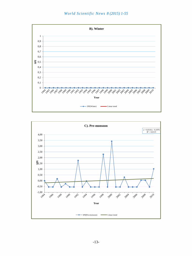
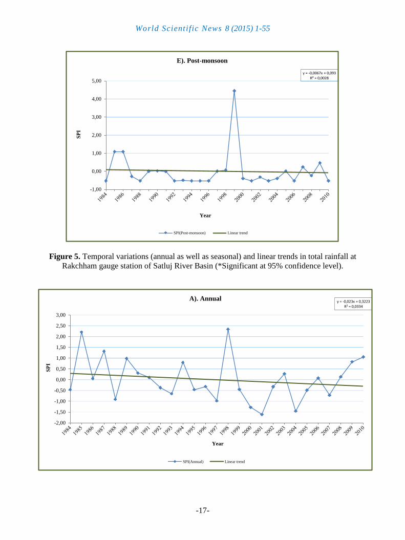
The Figure 5 indicates that the annual rainfall has shown increasing trend which is
statistically significant, with episodic fluctuations. Seasonal analysis shows that maximum
increasing trend was observed during pre-monsoon, followed by winter and monsoon
respectively which are statistically significant, while the post-monsoon has insignificantly
decreasing trend. The analysis shows overall increasing trend in the rainfall pattern.
y = 0.072x - 1.014 R² = 0.330*
-2,00
-1,50
-1,00
-0,50
0,00
0,50
1,00
1,50
2,00
2,50
3,00
SP
I
Year
A). Annual
SPI(Annual) Linear trend
y = 0.055x - 0.780 R² = 0.196*
-1,00
0,00
1,00
2,00
3,00
4,00
5,00
SP
I
Year
B). Winter
SPI(Winter) Linear trend

World Scientific News 8 (2015) 1-55
-16-
y = 0.047x - 0.661
R² = 0.140*
-2,50
-2,00
-1,50
-1,00
-0,50
0,00
0,50
1,00
1,50
2,00
2,50
3,00
SP
I
Year
D). Monsoon
SPI(Monsoon) Linear trend
y = 0.058x - 0.823 R² = 0.218*
-2,00
-1,00
0,00
1,00
2,00
3,00
4,00
SP
I
Year
C). Pre-monsoon
SPI(Pre-monsoon) Linear trend
World Scientific News 8 (2015) 1-55
-17-
Figure 5. Temporal variations (annual as well as seasonal) and linear trends in total rainfall at
Rakchham gauge station of Satluj River Basin (*Significant at 95% confidence level).
y = -0,0067x + 0,093 R² = 0,0028
-1,00
0,00
1,00
2,00
3,00
4,00
5,00S
PI
Year
E). Post-monsoon
SPI(Post-monsoon) Linear trend
y = -0,023x + 0,3223 R² = 0,0334
-2,00
-1,50
-1,00
-0,50
0,00
0,50
1,00
1,50
2,00
2,50
3,00
SP
I
Year
A). Annual
SPI(Annual) Linear trend

World Scientific News 8 (2015) 1-55
-18-
y = -0,039x + 0,5457 R² = 0,0957
-1,50
-1,00
-0,50
0,00
0,50
1,00
1,50
2,00
2,50
3,00
3,50
SP
I
Year
B). Winter
SPI(Winter) Linear trend
y = -0,0323x + 0,4528 R² = 0,0659
-1,50
-1,00
-0,50
0,00
0,50
1,00
1,50
2,00
2,50
3,00
SP
I
Year
C). Pre-monsoon
SPI(Pre-monsoon) Linear trend
World Scientific News 8 (2015) 1-55
-19-
Figure 6. Temporal variations (annual as well as seasonal) and linear trends in total rainfall at Namgia
gauge station of Satluj River Basin.
y = 0,0201x - 0,2817 R² = 0,0255
-2,00
-1,50
-1,00
-0,50
0,00
0,50
1,00
1,50
2,00
2,50
SP
I
Year
D). Monsoon
SPI(Monsoon) Linear trend
y = -0,0107x + 0,1499 R² = 0,0072
-1,00
0,00
1,00
2,00
3,00
4,00
5,00
SP
I
Year
E). Post-monsoon
SPI(Post-monsoon) Linear trend

World Scientific News 8 (2015) 1-55
-20-
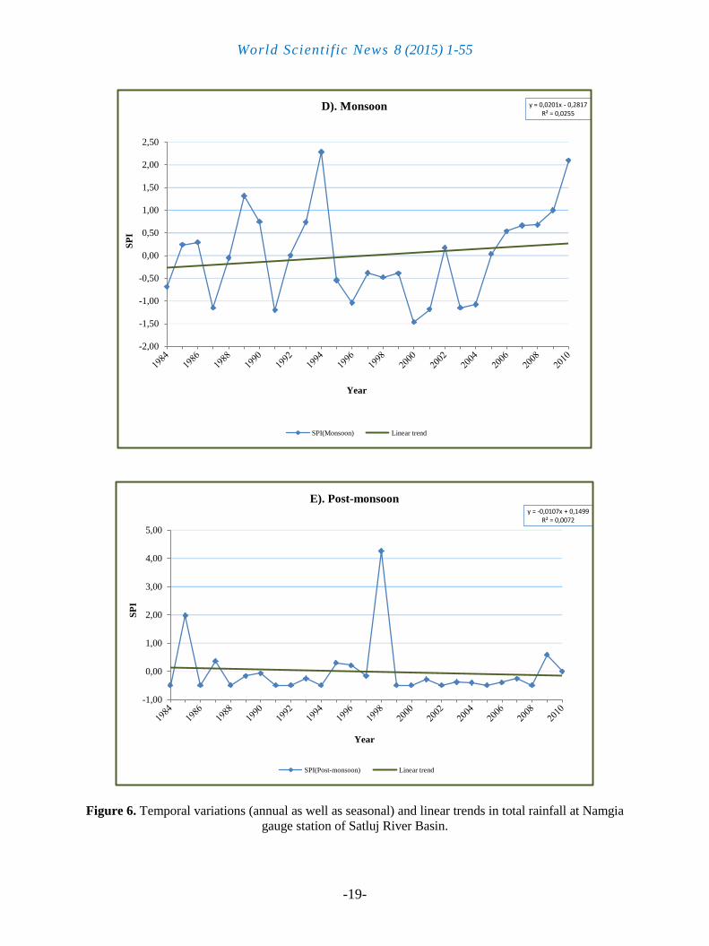
The Figure 6 indicates that the annual rainfall has shown decreasing trend but
statistically insignificant, with episodic fluctuations. Seasonal analysis shows that maximum
decreasing trend was observed during winter, followed by pre-monsoon and post-monsoon
but all are statistically insignificant, while the monsoon has shown increasing trend which is
statistically insignificant.
y = 0,0184x - 0,2573
R² = 0,0213
-1,50
-1,00
-0,50
0,00
0,50
1,00
1,50
2,00
2,50
3,00
SP
I
Year
A). Annual
SPI(Annual) Linear trend
y = -0,0297x + 0,4162
R² = 0,0556
-1,50
-1,00
-0,50
0,00
0,50
1,00
1,50
2,00
2,50
3,00
SP
I
Year
B). Winter
SPI(Winter) Linear trend

World Scientific News 8 (2015) 1-55
-21-
y = -0,0012x + 0,0169 R² = 9E-05
-1,50
-1,00
-0,50
0,00
0,50
1,00
1,50
2,00
2,50
3,00S
PI
Year
C). Pre-monsoon
SPI(Pre-monsoon) Linear trend
y = 0.059x - 0.835 R² = 0.224*
-2,00
-1,50
-1,00
-0,50
0,00
0,50
1,00
1,50
2,00
2,50
SP
I
Year
D). Monsoon
SPI(Monsoon) Linear trend

World Scientific News 8 (2015) 1-55
-22-
Figure 7. Temporal variations (annual as well as seasonal) and linear trends in total rainfall at Kalpa
gauge station of Satluj River (*Significant at 95% confidence level).
The Figure 7 indicates that the annual rainfall has shown increasing trend which is
statistically insignificant with episodic fluctuations. The slightly decreasing trend was
observed during winter and post-monsoon but statistically insignificant, while the pre-
monsoon has shown no trend. The monsoon season has shown increasing trend which is
statistically significant, having very high r2
value.
y = -0,0199x + 0,2782 R² = 0,0249
-1,00
-0,50
0,00
0,50
1,00
1,50
2,00
2,50
3,00
3,50
4,00S
PI
Year
E). Post-monsoon
SPI(Post-monsoon) Linear trend
y = -0.059x + 0.741 R² = 0.175*
-2,00
-1,50
-1,00
-0,50
0,00
0,50
1,00
1,50
2,00
2,50
3,00
3,50
SP
I
Year
A). Annual
SPI(Annual) Linear trend

World Scientific News 8 (2015) 1-55
-23-
y = -0,0325x + 0,4065 R² = 0,0529
-1,50
-1,00
-0,50
0,00
0,50
1,00
1,50
2,00
2,50S
PI
Year
B). Winter
SPI(Winter) Linear trend
y = -0,0089x + 0,1111 R² = 0,0039
-2,00
-1,50
-1,00
-0,50
0,00
0,50
1,00
1,50
2,00
2,50
SP
I
Year
C). Pre-monsoon
SPI(Pre-monsoon) Linear trend

World Scientific News 8 (2015) 1-55
-24-
Figure 8. Temporal variations (annual as well as seasonal) and linear trends in total rainfall at
Swarghat gauge station of Satluj River Basin (*Significant at 95% confidence level).
y = -0,0544x + 0,6798 R² = 0,1479
-2,00
-1,00
0,00
1,00
2,00
3,00
4,00S
PI
Year
D). Monsoon
SPI(Monsoon) Linear trend
y = -0,0242x + 0,3021 R² = 0,0292
-1,00
-0,50
0,00
0,50
1,00
1,50
2,00
2,50
SP
I
Year
E). Post-monsoon
SPI(Post-monsoon) Linear trend

World Scientific News 8 (2015) 1-55
-25-
The Figure 8 indicates that the annual rainfall has shown decreasing trend which is
statistically significant. Seasonal analysis shows that maximum decreasing trend was
observed during monsoon, followed by winter, post-monsoon and pre-monsoon but all are
statistically insignificant. The overall analysis shows decreasing trend with the exception of
some periodic behaviour.
y = 0,0345x - 0,4829
R² = 0,0749
-2,00
-1,50
-1,00
-0,50
0,00
0,50
1,00
1,50
2,00
2,50
3,00
SP
I
Year
A). Annual
SPI(Annual) Linear trend
y = -0,0313x + 0,4384
R² = 0,0618
-2,50
-2,00
-1,50
-1,00
-0,50
0,00
0,50
1,00
1,50
2,00
2,50
3,00
SP
I
Year
B). Winter
SPI(Winter) Linear trend

World Scientific News 8 (2015) 1-55
-26-
y = 0,0437x - 0,612
R² = 0,1203
-2,00
-1,50
-1,00
-0,50
0,00
0,50
1,00
1,50
2,00
2,50S
PI
Year
C). Pre-monsoon
SPI(Pre-monsoon) Linear trend
y = 0,0431x - 0,6029
R² = 0,1168
-2,50
-2,00
-1,50
-1,00
-0,50
0,00
0,50
1,00
1,50
2,00
2,50
SP
I
Year
D). Monsoon
SPI(Monsoon) Linear trend

World Scientific News 8 (2015) 1-55
-27-
Figure 9. Temporal variations (annual as well as seasonal) and linear trends in total rainfall at Rampur
gauge station of Satluj River Basin.
The Figure 9 indicates that the annual rainfall has shown increasing trend which is
statistically insignificant with episodic fluctuations. The increasing trend was observed during
pre-monsoon, followed by monsoon but statistically insignificant. The winter season has
shown decreasing trend, followed by post-monsoon which are statistically insignificant.
y = -0,0142x + 0,1988
R² = 0,0127
-1,50
-1,00
-0,50
0,00
0,50
1,00
1,50
2,00
2,50S
PI
Year
E). Post-monsoon
SPI(Post-monsoon) Linear trend
y = 0,0142x - 0,1989
R² = 0,0127
-2,50
-2,00
-1,50
-1,00
-0,50
0,00
0,50
1,00
1,50
2,00
2,50
SP
I
Year
A). Annual
SPI(Annual) Linear trend

World Scientific News 8 (2015) 1-55
-28-
y = -0,0356x + 0,4979
R² = 0,0797
-2,00
-1,50
-1,00
-0,50
0,00
0,50
1,00
1,50
2,00
2,50
3,00
3,50
SP
I
Year
B). Winter
SPI(Winter) Linear trend
y = 0,0281x - 0,3932
R² = 0,0497
-1,50
-1,00
-0,50
0,00
0,50
1,00
1,50
2,00
2,50
3,00
SP
I
Year
C). Pre-monsoon
SPI(Pre-monsoon) Linear trend

World Scientific News 8 (2015) 1-55
-29-
Figure 10. Temporal variations (annual as well as seasonal) and linear trends in total rainfall at Suni
gauge station of Satluj River.
y = 0,0193x - 0,2707
R² = 0,0236
-2,00
-1,50
-1,00
-0,50
0,00
0,50
1,00
1,50
2,00
2,50
3,00
SP
I
Year
D). Monsoon
SPI(Monsoon) Linear trend
y = -0,0117x + 0,1631
R² = 0,0086
-1,50
-1,00
-0,50
0,00
0,50
1,00
1,50
2,00
2,50
3,00
3,50
SP
I
Year
E). Post-monsoon
SPI(Post-monsoon) Linear trend

World Scientific News 8 (2015) 1-55
-30-
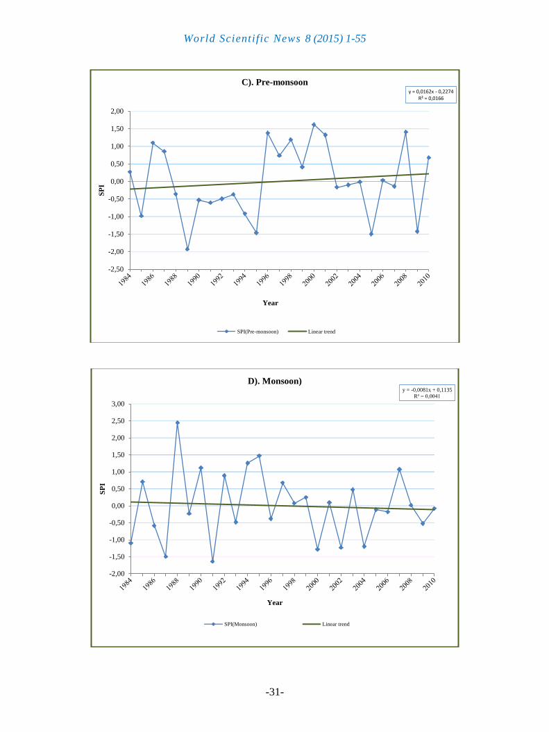
The Figure 10 indicates that the annual rainfall has shown increasing trend which is
statistically insignificant with episodic fluctuations. The increasing trend was observed during
pre-monsoon, followed by monsoon but statistically insignificant. The winter season displays
a decreasing trend, followed by post-monsoon which are statistically insignificant.
y = -0,0215x + 0,3006
R² = 0,029
-2,00
-1,50
-1,00
-0,50
0,00
0,50
1,00
1,50
2,00
2,50
SP
I
Year
A). Annual
SPI(Annual) Linear trend
y = -0,042x + 0,5884
R² = 0,1113
-2,00
-1,00
0,00
1,00
2,00
3,00
4,00
5,00
SP
I
Year
B). Winter
SPI(Winter) Linear trend
World Scientific News 8 (2015) 1-55
-31-
y = 0,0162x - 0,2274 R² = 0,0166
-2,50
-2,00
-1,50
-1,00
-0,50
0,00
0,50
1,00
1,50
2,00
SP
I
Year
C). Pre-monsoon
SPI(Pre-monsoon) Linear trend
y = -0,0081x + 0,1135
R² = 0,0041
-2,00
-1,50
-1,00
-0,50
0,00
0,50
1,00
1,50
2,00
2,50
3,00
SP
I
Year
D). Monsoon)
SPI(Monsoon) Linear trend

World Scientific News 8 (2015) 1-55
-32-
Figure 11. Temporal variations (annual as well as seasonal) and linear trends in total rainfall at Kasol
gauge station of Satluj River.
The Figure 11 indicates that the annual rainfall has shown decreasing trend which is
statistically insignificant. Seasonal analysis shows that maximum decreasing trend was
observed during winter, followed by post-monsoon and monsoon but all are statistically
insignificant. Although increasing trend was observed during pre-monsoon but statistically
insignificant. The overall analysis shows decreasing trend with the exception of some periodic
behaviour.
y = -0,0303x + 0,4237
R² = 0,0577
-1,00
-0,50
0,00
0,50
1,00
1,50
2,00
2,50
3,00S
PI
Year
E). Post-monsoon
SPI(Post-monsoon) Linear trend
y = -0,0302x + 0,3712
R² = 0,051
-2,00
-1,50
-1,00
-0,50
0,00
0,50
1,00
1,50
2,00
SP
I
Year
A). Annual
SPI(Annual) Linear trend

World Scientific News 8 (2015) 1-55
-33-
y = -0,0299x + 0,3729 R² = 0,0502
-2,00
-1,50
-1,00
-0,50
0,00
0,50
1,00
1,50
2,00S
PI
Year
B). Winter
SPI(Winter) Linear trend
y = 0,0104x - 0,1488 R² = 0,0061
-2,00
-1,50
-1,00
-0,50
0,00
0,50
1,00
1,50
2,00
2,50
SP
I
Year
C). Pre-monsoon
SPI(Pre-monsoon) Linear trend

World Scientific News 8 (2015) 1-55
-34-
Figure 12. Temporal variations (annual as well as seasonal) and linear trends in total rainfall at
Daslehra gauge station of Satluj River Basin.
y = -0,0256x + 0,3226 R² = 0,0368
-2,00
-1,50
-1,00
-0,50
0,00
0,50
1,00
1,50
2,00
2,50
SP
I
Year
D). Monsoon
SPI(Monsoon) Linear trend
y = -0,0233x + 0,2736 R² = 0,0301
-1,00
-0,50
0,00
0,50
1,00
1,50
2,00
2,50
SP
I
Year
E). Post-monsoon
SPI(Post-monsoon) Linear trend

World Scientific News 8 (2015) 1-55
-35-
The Figure 12 indicates that the annual rainfall has shown decreasing trend which is
statistically insignificant. Seasonal analysis shows that maximum decreasing trend was
observed during winter, followed by monsoon and post-monsoon but all are statistically
insignificant. Although increasing trend was observed during pre-monsoon but statistically
insignificant. The overall analysis shows decreasing trend with the exception of some periodic
behaviour.
y = 0,0409x - 0,5111 R² = 0,0836
-2,00
-1,50
-1,00
-0,50
0,00
0,50
1,00
1,50
2,00
2,50
SP
I
Year
A). Annual
SPI(Annual) Linear trend
y = 0.061x - 0.773 R² = 0.191*
-1,50
-1,00
-0,50
0,00
0,50
1,00
1,50
2,00
2,50
3,00
3,50
SP
I
Year
B). Winter
SPI(Winter) Linear trend

World Scientific News 8 (2015) 1-55
-36-
y = 0,0084x - 0,1047 R² = 0,0035
-2,00
-1,50
-1,00
-0,50
0,00
0,50
1,00
1,50
2,00
2,50
3,00
SP
I
Year
C). Pre-monsoon
SPI(Pre-monsoon) Liniowy (SPI(Pre-monsoon))
y = 0,0258x - 0,3219
R² = 0,0332
-3,00
-2,50
-2,00
-1,50
-1,00
-0,50
0,00
0,50
1,00
1,50
2,00
2,50
SP
I
Year
D). Monsoon
SPI(Monsoon) Linear trend

World Scientific News 8 (2015) 1-55
-37-
Figure 13. Temporal variations (annual as well as seasonal) and linear trends in total rainfall at Naina
Devi gauge station of Satluj River Basin (*Significant at 95% confidence level).
The Figure 13 indicates that the annual rainfall has shown increasing trend but
statistically insignificant with episodic fluctuations. Seasonal analysis shows that maximum
increasing trend was observed during winter which is statistically significant, followed by
monsoon and pre-monsoon but statistically insignificant, while the post-monsoon season has
no trend. The analysis shows overall increasing trend in the rainfall pattern.
y = -0,0035x + 0,0434
R² = 0,0006
-1,00
-0,50
0,00
0,50
1,00
1,50
2,00
2,50
3,00
3,50S
PI
Year
E). Post-monsoon
SPI(Post-monsoon) Linear trend
y = -0,0464x + 0,6493 R² = 0,1355
-2,00
-1,50
-1,00
-0,50
0,00
0,50
1,00
1,50
2,00
2,50
3,00
SP
I
Year
A). Annual
SPI(Annual) Linear trend

World Scientific News 8 (2015) 1-55
-38-
y = -0.048x + 0.684 R² = 0.150*
-2,00
-1,00
0,00
1,00
2,00
3,00
4,00S
PI
Year
B). Winter
SPI(Winter) Linear trend
y = -0,0013x + 0,0175 R² = 1E-04
-2,50
-2,00
-1,50
-1,00
-0,50
0,00
0,50
1,00
1,50
2,00
2,50
SP
I
Year
C). Pre-monsoon
SPI(Pre-monsoon) Linear trend

World Scientific News 8 (2015) 1-55
-39-
Figure 14. Temporal variations (annual as well as seasonal) and linear trends in total rainfall at
Berthin gauge station of Satluj River Basin (*Significant at 95% confidence level).
y = -0,0279x + 0,3906 R² = 0,049
-3,00
-2,00
-1,00
0,00
1,00
2,00
3,00
4,00
SP
I
Year
D). Monsoon
SPI(Monsoon) Linear trend
y = -0,0291x + 0,408 R² = 0,0535
-1,00
-0,50
0,00
0,50
1,00
1,50
2,00
2,50
3,00
SP
I
Year
E). Post-monsoon
SPI(Post-monsoon) Linear trend

World Scientific News 8 (2015) 1-55
-40-
The Figure 14 indicates that the annual rainfall has shown decreasing trend which is
statistically insignificant. Seasonal analysis shows that maximum decreasing trend was
observed during winter which is statistically significant, followed by post-monsoon and
monsoon but statistically insignificant. Almost no trend was observed during pre-monsoon
season. The overall analysis shows decreasing trend with the exception of some periodic
behaviour.
y = -0.062x + 0.874 R² = 0.245*
-2,00
-1,50
-1,00
-0,50
0,00
0,50
1,00
1,50
2,00
2,50
3,00
SP
I
Year
A). Annual
SPI(Annual) Linear trend
y = -0.048x + 0.679
R² = 0.148*
-2,50
-2,00
-1,50
-1,00
-0,50
0,00
0,50
1,00
1,50
2,00
2,50
SP
I
Year
B). Winter
SPI(Winter) Linear trend

World Scientific News 8 (2015) 1-55
-41-
y = -0,0286x + 0,4007
R² = 0,0516
-2,00
-1,50
-1,00
-0,50
0,00
0,50
1,00
1,50
2,00
2,50
3,00S
PI
Year
C). Pre-monsoon
SPI(Pre-monsoon) Linear trend
y = -0,0448x + 0,6279
R² = 0,1267
-2,00
-1,50
-1,00
-0,50
0,00
0,50
1,00
1,50
2,00
2,50
SP
I
Year
D). Monsoon
SPI(Monsoon) Linear trend
World Scientific News 8 (2015) 1-55
-42-
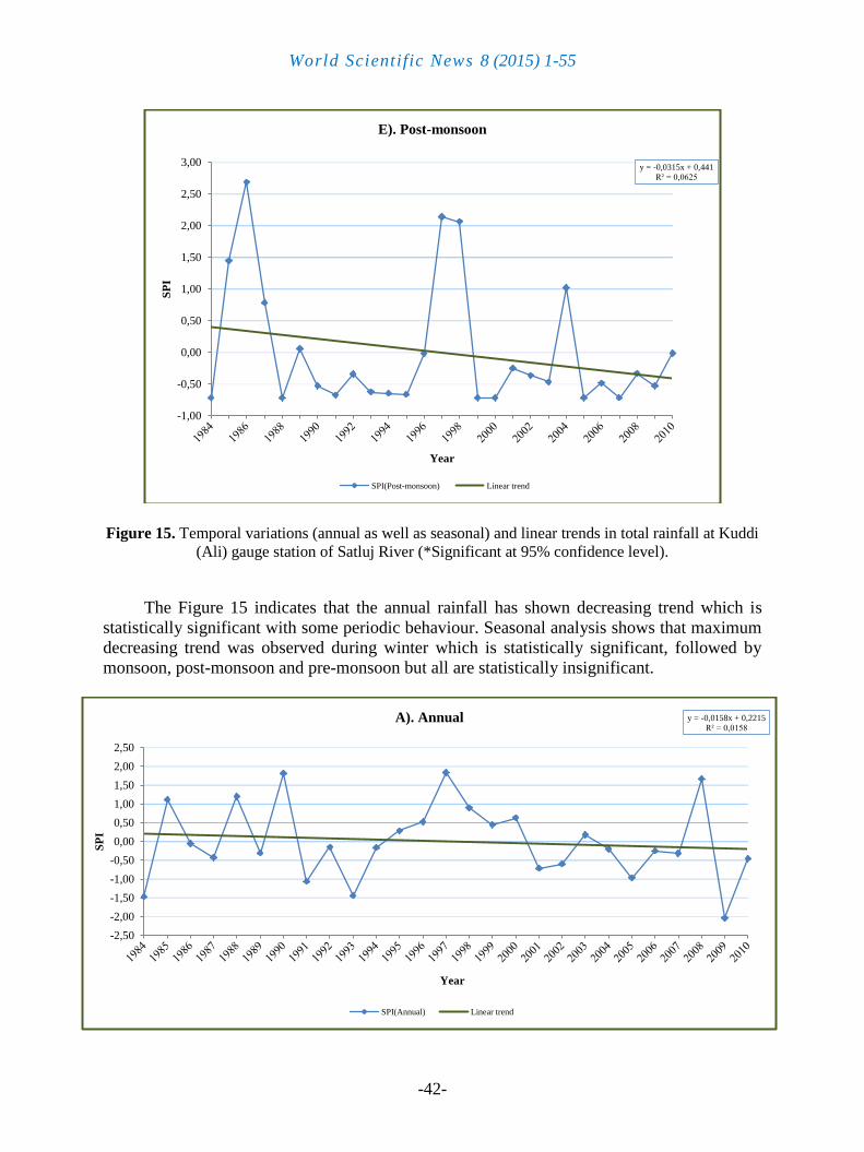
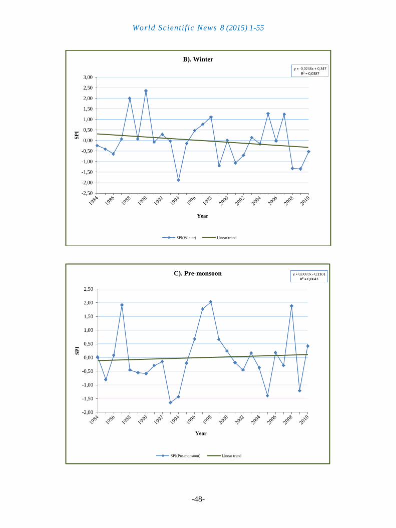
Figure 15. Temporal variations (annual as well as seasonal) and linear trends in total rainfall at Kuddi
(Ali) gauge station of Satluj River (*Significant at 95% confidence level).
The Figure 15 indicates that the annual rainfall has shown decreasing trend which is
statistically significant with some periodic behaviour. Seasonal analysis shows that maximum
decreasing trend was observed during winter which is statistically significant, followed by
monsoon, post-monsoon and pre-monsoon but all are statistically insignificant.
y = -0,0315x + 0,441
R² = 0,0625
-1,00
-0,50
0,00
0,50
1,00
1,50
2,00
2,50
3,00S
PI
Year
E). Post-monsoon
SPI(Post-monsoon) Linear trend
y = -0,0158x + 0,2215
R² = 0,0158
-2,50
-2,00
-1,50
-1,00
-0,50
0,00
0,50
1,00
1,50
2,00
2,50
SP
I
Year
A). Annual
SPI(Annual) Linear trend

World Scientific News 8 (2015) 1-55
-43-
y = -0,0335x + 0,4687 R² = 0,0706
-2,00
-1,50
-1,00
-0,50
0,00
0,50
1,00
1,50
2,00
2,50
3,00S
PI
Year
B). Winter
SPI(Winter) Linear trend
y = 0,0347x - 0,4859 R² = 0,0759
-1,50
-1,00
-0,50
0,00
0,50
1,00
1,50
2,00
2,50
3,00
SP
I
Year
C). Pre-monsoon
SPI(Pre-monsoon) Linear trend

World Scientific News 8 (2015) 1-55
-44-
Figure 16. Temporal variations (annual as well as seasonal) and linear trends in total rainfall at Kahu
gauge station of Satluj River.
y = -0,0175x + 0,2445 R² = 0,0192
-2,00
-1,50
-1,00
-0,50
0,00
0,50
1,00
1,50
2,00
2,50S
PI
Year
D). Monsoon
SPI(Monsoon) Linear trend
y = -0,0226x + 0,3159 R² = 0,0321
-1,00
-0,50
0,00
0,50
1,00
1,50
2,00
2,50
SP
I
Year
E). Post-monsoon
SPI(Post-monsoon) Linear trend

World Scientific News 8 (2015) 1-55
-45-
The Figure 16 indicates that the annual rainfall has shown decreasing trend which is
statistically insignificant. Seasonal analysis shows that maximum decreasing trend was
observed during winter, followed by post-monsoon and monsoon but all are statistically
insignificant. Although increasing trend was observed during pre-monsoon but statistically
insignificant. The overall analysis shows decreasing trend with the exception of some periodic
behaviour.
y = 0,0024x - 0,1195 R² = 0,0004
-2,00
-1,50
-1,00
-0,50
0,00
0,50
1,00
1,50
2,00
2,50
3,00
SP
I
Year
A). Annual
SPI(Annual) Linear trend
y = -0,0011x - 0,0942 R² = 7E-05
-2,00
-1,50
-1,00
-0,50
0,00
0,50
1,00
1,50
2,00
2,50
SP
I
Year
B). Winter
SPI(Winter) Linear trend

World Scientific News 8 (2015) 1-55
-46-
y = -0,0001x - 0,0272 R² = 1E-06
-2,00
-1,50
-1,00
-0,50
0,00
0,50
1,00
1,50
2,00
2,50
3,00
SP
I
Year
C). Pre-monsoon
SPI(Pre-monsoon) Linear trend
y = 0,0064x - 0,167 R² = 0,0026
-2,00
-1,50
-1,00
-0,50
0,00
0,50
1,00
1,50
2,00
SP
I
Year
D). Monsoon
SPI(Monsoon) Linear trend

World Scientific News 8 (2015) 1-55
-47-
Figure 17. Temporal variations (annual as well as seasonal) and linear trends in total rainfall at
Bilaspur gauge station of Satluj River Basin.
The Figure 17 indicates that the annual rainfall has shown almost no trend with the
exception of some episodic fluctuations. The figures also show slightly increasing and
decreasing trends during monsoon and post-monsoon respectively but statistically
insignificant. Almost no trend was observed during winter and pre-monsoon. The overall
analysis shows no trend with the exception of some periodic behaviour.
y = -0,0089x + 0,1323 R² = 0,0052
-1,00
-0,50
0,00
0,50
1,00
1,50
2,00
2,50
3,00
3,50S
PI
Year
E). Post-monsoon
SPI(Post-monsoon) Linear trend
y = -0,0417x + 0,5841 R² = 0,1097
-2,00
-1,50
-1,00
-0,50
0,00
0,50
1,00
1,50
2,00
2,50
3,00
3,50
SP
I
Year
A). Annual
SPI(Annual) Linear trend
World Scientific News 8 (2015) 1-55
-48-
y = -0,0248x + 0,347 R² = 0,0387
-2,50
-2,00
-1,50
-1,00
-0,50
0,00
0,50
1,00
1,50
2,00
2,50
3,00S
PI
Year
B). Winter
SPI(Winter) Linear trend
y = 0,0083x - 0,1161 R² = 0,0043
-2,00
-1,50
-1,00
-0,50
0,00
0,50
1,00
1,50
2,00
2,50
SP
I
Year
C). Pre-monsoon
SPI(Pre-monsoon) Linear trend

World Scientific News 8 (2015) 1-55
-49-
Figure 18. Temporal variations (annual as well as seasonal) and linear trends in total rainfall at
Bhakra gauge station of Satluj River.
y = -0,0443x + 0,6197 R² = 0,1234
-1,50
-1,00
-0,50
0,00
0,50
1,00
1,50
2,00
2,50
3,00
3,50S
PI
Year
D). Monsoon
SPI(Monsoon) Linear trend
y = -0,0217x + 0,3042
R² = 0,0297
-1,00
-0,50
0,00
0,50
1,00
1,50
2,00
2,50
3,00
SP
I
Year
E). Post-monsoon
SPI(Post-monsoon) Linear trend

World Scientific News 8 (2015) 1-55
-50-
The Figure 18 indicates that the annual rainfall has followed a decreasing trend which is
statistically insignificant. Seasonal analysis shows that maximum decreasing trend was
observed during monsoon, followed by winter and post-monsoon but all are statistically
insignificant. Although slightly increasing but statistically insignificant trend was observed
during pre-monsoon. The overall analysis shows decreasing trend with the exception of some
episodic fluctuations.
Table 2. Results of trend analysis of rainfall in Satluj River Basin.
S. No. Station Trend analysis
Mann-Kendall Linear regression
A S1 S2 S3 S4 A S1 S2 S3 S4
1. Kaza -(.70) -- +(.62) -(.50) +(.95) -(.56) -- +(.57) -(.47) +(.90)
2. Rakchham +(.00)* +(.01)* +(.04)* +(.04)* -(.93) +(.00)* +(.02)* +(.01)* +(.05)* -(.79)
3. Namgia -(.51) -(.29) -(.50) +(.36) -(1.00) -(.36) -(.12) -(.20) +(.43) -(.67)
4. Kalpa +(.68) -(.57) -(.90) +(.03)* -(.80) +(.47) -(.24) -(.96) +(.01)* -(.43)
5. Swarghat -(.05)* -(.27) -(.64) -(.07) -(.88) -(.04)* -(.28) -(.77) -(.06) -(.42)
6. Rampur +(.56) -(.41) +(.06) +(.26) -(.87) +(.16) -(.21) +(.07) +(.08) -(.57)
7. Suni +(.80) -(.34) +(.28) +(.25) -(.68) +(.57) -(.15) +(.26) +(.44) -(.65)
8. Kasol -(.31) -(.07) +(.41) -(.87) -(.80) -(.39) -(.09) +(.52) -(.75) -(.23)
9.Daslehra -(.32) -(.30) +(.98) -(.39) -(.27) -(.28) -(.29) +(.71) -(.36) -(.41)
10. Naina Devi+(.12) +(.04)* +(.84) +(.71) -(.88) +(.17) +(.03)* +(.78) +(.39) -(.90)
11. Berthin -(.10) -(.05)* -(.98) -(.46) -(.60) -(.06) -(.04)* -(.96) -(.27) -(.25)
12. Kuddi -(.01)* -(.03)* -(.41) -(.17) -(.87) -(.01)* -(.05)* -(.25) -(.07) -(.21)
13. Kahu -(.46) -(.19) +(.26) -(.54) -(.98) -(.53) -(.18) +(.16) -(.49) -(.37)
14. Bilaspur +(1.00) -(.71) -(.97) +(.97) -(.34) +(.92) -(.97) -(.99) +(.80) -(.72)
15. Bhakra -(.10) -(.51) +(.56) -(.11) -(.55) -(.09) -(.32) +(.74) -(.07) -(.39)
*Significance at 95% confidence level. (+) increasing, (-) decreasing.
A: Annual, S1: Winter; S2: Pre-monsoon; S3: Monsoon; S4: Post-monsoon
The trend analysis results (Table 2) of rainfall through non-parametric Mann-Kendall
and parametric linear regression tests indicate that the annual rainfall at Rakchham, Kalpa,
Rampur, Suni, Naina Devi and Bilaspur shows increasing but Kaza, Namgia, Swarghat,
Kasol, Daslehra, Berthin, Kuddi, Kahu and Bhakra show decreasing trends. Out of them, only
Rakchham is statistically significant (increasing) and Swarghat and Kuddi are statistically
significant (decreasing) at 95% confidence level. During winter, Rakchham and Naina Devi
display increasing trends which are statistically significant.
Kalpa, Namgia, Swarghat, Rampur, Suni, Kasol, Bilaspur, Daslehra, Berthin, Kuddi,
Kahu and Bhakra show decreasing trends where only Berthin and Kuddi are statistically
significant. During pre-monsoon, Kaza, Rakchham, Rampur, Suni, Kasol, Daslehra, Naina
Devi, Kahu and Bhakra show increasing where only Rakchham shows statistically significant
trend. But Namgia, Kalpa, Swarghat, Berthin, Kuddi and Bilaspur show statistically

World Scientific News 8 (2015) 1-55
-51-
insignificant decreasing trends. During monsoon, Rakchham, Namgia, Kalpa, Rampur, Suni,
Naina Devi and Bilaspur show increasing where only Rakchham and Kalpa show statistically
significant trends. But Kaza, Swarghat, Kasol, Daslehra, Berthin, Kuddi, Kahu and Bhakra
has shown statistically insignificant decreasing trends. During post-monsoon, only Kaza
shows increasing and statistically insignificant trend. Rakchham, Namgia, Kalpa, Rampur,
Suni, Swarghat, Kasol, Naina Devi, Bilaspur, Daslehra, Berthin, Kuddi, Kahu and Bhakra
show decreasing trends which are statistically insignificant.
Table 3. Trend test results of rainfall.
Seasons No. of No. of increasing % No. of decreasing %
trends trends (significant) (sign) trends (significant) (sign)
Annual 15 6(1) 40(6.6) 9(2) 60(13.3)
Winter 15 2(2) 13.3(13.3) 13(2) 86.6(13.3)
Pre-monsoon 15 9(1) 60(6.6) 6(0) 40(0)
Monsoon 15 7(2) 46.6(13.3) 8(0) 53.9(0)
Post-monsoon 15 1(0) 6.6(0) 14(0) 73.3(0)
# Significance at 95% confidence level.
Trend analysis results of rainfall (Table 3) show that out of 15 annual trends 6 (40%)
are increasing and 9 (60%) are decreasing in nature where 1 (6.6%) is statistically significant
(increasing) and 2 (13.3%) are statistically significant (decreasing) at 95% confidence level.
During winter, 2 (13.3%) are showing statistically significant increasing trend but 13 (86.6%)
are showing decreasing trends where 2 (13.3%) are statistically significant. During pre-
monsoon, 9 (60%) are increasing but 6 (40%) are decreasing in nature where only 1 (6.6%) is
statistically significant (increasing). During monsoon, 7 (46.6%) are showing increasing
where 2 (13.3%) are statistically significant. But 8 (53.9%) are showing decreasing trends
where all are statistically significant at 95% confidence level. During post-monsoon, only 1
(6.6%) is increasing but statistically significant. 14 (73.3%) are decreasing in nature where
none is statistically significant.
The results indicate remarkable differences among the observation stations with
negative and positive trends. The trends found by the linear regression were almost similar to
Mann-Kendall test. The analysis shows mixed patterns of change where only few data series
has significant trends. The rainfall at some gauge stations showed statistically significant
increasing trends at the 95% confidence levels. The analysis indicates episodic fluctuations in
rainfall pattern which may have been caused due to changing climatic conditions. The uneven
distribution of rain, its intensity and periodicity, shows the irregular pattern at various
locations. The analysis shows that the study area reveals significant increasing/decreasing
trends in rainfall, at 95% confidence level, appear to have a response to climate change. The
analysis of annual as well as seasonal rainfall for the Satluj River Basin indicates significant
changes from 1984 to 2010. There is a clear contrast in the rainfall pattern between the high
and low altitude mountainous region where the orographic effect plays a significant role.
Shifts in climatic regimes, particularly precipitation, in space and time, would impact
heavily on the river systems originating in mountain areas (Beniston et al., 1997) like Satluj

World Scientific News 8 (2015) 1-55
-52-
River Basin. The sensitivity of rainfall variations provides important insight regarding the
responses and vulnerability of such mountainous areas to the vagaries of climate change. Due
to climate change, the rainfall patterns are changing. The monsoons penetrating deeper into
the cold deserts in Satluj River Basin have become a matter of concern. Shifts of precipitation
in the form of rainfall towards upstream could have major environmental consequences. The
influence of climate change on hydrologic processes, especially in mountain basins is
paramount for understanding, forecasting and mitigating water related hazards. The impacts
of climatic change in the form of irregular precipitation and increased intensity and frequency
of the flooding events, likely became obstacles to the sustainable development of a life-
sustaining system.
5. CONCLUSIONS
Trend analysis of historical data concluded that the spatial and temporal variations in
rainfall pattern are due to climate change. The rainfall in the basin shows great temporal and
spatial variations, unequal seasonal and geographical distribution with frequent departures
from normal. The monsoons penetrating deeper into the cold deserts in Satluj River Basin
have become a matter of concern. It is predicted that the glaciers will receive more
precipitation in the form of rainfall rather than snowfall. Shifts of precipitation in the form of
rainfall towards upstream could have major environmental consequences. Information from
trend analysis will be useful in the planning, development and management of water resources
in the study area. Densification of rainfall gauge stations will further strengthen the
formulation of future strategy for the management of river catchment area.
Acknowledgements
Authors are thankful to Indian Council of Medical Research (ICMR) and University Grant Commission (UGC),
New Delhi for providing financial assistance in the form of research fellowship.
References
[1] Archer DR and Fowler HJ (2004) Spatial and temporal variations in precipitation in the
Upper Indus Basin, global teleconnections and hydrological implications, Hydrology
and Earth System Sciences, 8: 47-61.
[2] Bartarya SK, Virdi NS and Sah MP (1996) Landslide hazards: Some case studies from
the Satluj Valley, Himachal Pradesh: Himalayan Geology, 17: 193-207.
[3] Bayazit M and Önöz B (2007) To pre-whiten or not to pre-whiten in trend analysis?
Hydrological Sciences Journal, 52 (4): 611-624.
[4] Beniston M, Diaz FD and Bradley RS (1997) Climate change at high elevation sites: An
overview, Climate Change, 36: 233-251.
World Scientific News 8 (2015) 1-55
-53-
[5] Bhutiyani MR, Kale VS and Pawar NJ (2008) Changing streamflow patterns in the
rivers of northwestern Himalaya: Implications of global warming in the 20th
century,
Current Science, 95 (5): 618-626.
[6] Buffoni L, Maugeri M and Nanni T (1999) Precipitation in Italy from 1833 to 1996,
Theoretical and Applied Climatology, 63: 33-40.
[7] Burn DH (1994) Hydrologic effects of climatic change in West-Central Canada, Journal
of Hydrology, 160: 53-70.
[8] Burn DH and Hag Elnur MA (2002) Detection of hydrologic trends and variability,
Journal of Hydrology, 255: 107-122.
[9] Burn DH, Cunderlik JM and Pietroniro A (2004) Hydrological trends and variability in
the Liard river basin, Hydrological Science Journal, 49: 53-67.
[10] Caloiero T, Coscarelli R, Ferrari E and Marco Mancini (2011) Trend detection of
annual and seasonal rainfall in Calabria (Southern Italy), International Journal of
Climatology, 31: 44-56.
[11] Cox DR and Stuart A (1955) Some quick sign tests for trend in location and dispersion,
Biometrika, 42: 80-95.
[12] Dietz EJ and Killeen TJ (1981) A nonparametric multivariate test for monotone trend
with pharmaceutical applications, Journal of the American Statistical Association, 76:
169-174.
[13] Dore MHI (2005) Climate change and changes in global precipitation patterns: What do
we know? Environmental International, 31: 1167-1181.
[14] Douglas EM, Vogel RM and Knoll CN (2000) Trends in flood and low flows in the
United States: impact of spatial correlation, Journal of Hydrology, 240: 90-105.
[15] Gilbert RO (1987) Statistical methods for environmental pollution monitoring, Van
Nostrand Reinhold, New York.
[16] Gupta V, Sah MP, Virdi NS and Bartarya SK (1994) Landslide hazard zonation in the
Upper Satluj Valley, District. Kinnaur, Himachal Pradesh, Journal of Himalayan
Geology, 4(1): 81-93.
[17] Hamilton JP, Whitelaw GS and Fenech A (2001) Mean annual temperature and annual
precipitation trends at Canadian biosphere reserves, Environmental Monitoring and
Assessment 67: 239-275.
[18] Helsel DR and Hirsch RM (1992) Statistical Methods in Water Resources, Elsevier,
New York.
[19] Hirsch RM and Slack JR (1984) Non-parametric trend test for seasonal data with serial
dependence, Water Resources Research, 20(6): 727-732.
[20] Hirsch RM, Slack JR and Smith RA (1982) Techniques of trend analysis for monthly
water quality data, Water Resources Research, 18: 107-121.

World Scientific News 8 (2015) 1-55
-54-
[21] Kampata JM, Parida BP and Moalafhi DB (2008) Trend analysis of rainfall in the
headstreams of the Zambezi River Basin in Zambia, Physics and Chemistry of the
Earth, 33: 621-625.
[22] Kendall MG (1975) Rank Correlation Methods, Griffin, London.
[23] Liu Q, Yang Z and Cui B (2008) Spatial and temporal variability of annual precipitation
during 1961–2006 in Yellow River Basin, China, Journal of Hydrology, 361: 330-338.
[24] Mann HB (1945) Nonparametric tests against trend, Econometrica 13: 245-259.
[25] Mooley DA and Parthasarathy B (1984) Fluctuations of All-India summer monsoon
rainfall during 1871-1978, Climatic Change, 6: 287-301.
[26] Partal T and Kahya E (2006) Trend analysis in Turkish precipitation data, Hydrological
Processes, 20: 2011-2026.
[27] Sharma KP, Moore III B and Vörösmarty CJ (2000) Sensitivity of the Himalayan
hydrology to land-use and climatic changes, Climate Change, 47: 117-139.
[28] Singh P, Kumar V, Thomas T and Arora M (2008) Changes in rainfall and relative
humidity in river basins in northwest and central India, Hydrological Processes, 22:
2982-2992.
[29] Sinha Ray KC and Srivastava AK (1999) Is there any change in extreme events like
droughts and heavy rainfall? INTROPMET-97, IIT New Delhi, 2-5 December, 1999.
[30] Tabari H and Marofi S (2010) Changes of pan evaporation in the West of Iran, Water
Resources Management, doi: 10.1007/s11269-010-9689-6.
[31] Tabari H and Talaee PH (2011) Temporal variability of precipitation over Iran: 1966–
2005, Journal of Hydrology, 396: 313-320.
[32] Tabari H, Marofi S and Ahmadi M (2010a) Long-term variations of water quality
parameters in the Maroon River, Iran, Environmental Monitoring and Assessment, doi:
10.1007/s10661-010-1633-y.
[33] Tabari H, Marofi S, Hosseinzadeh Talaee P and Mohammadi K (2010b) Trend analysis
of reference evapotranspiration in the western half of Iran, Agricultural and Forest
Meteorology, doi: 10.1016/j.agrformet.2010.09.009.
[34] Thapliyal V and Kulshrestha SM (1991) Climate changes and trends over India,
Mausam, 42: 333-338.
[35] Von Storch H (1995) Misuses of Statistical Analysis in Climate Research, In: Von
Storch H and Navarra A (eds.), Analysis of Climate Variability: Applications of
Statistical Techniques. Springer-Verlag, Berlin, pp. 11-26.
[36] Von Storch H and Navarra A (1995) Analysis of Climate Variability - Applications of
Statistical Techniques, Springer-Verlag: New York.
[37] Yu YS, Zou S and Whittemore D (1993) Non-parametric trend analysis of water quality
data of rivers in Kansas, Journal of Hydrology, 150: 61-80.

World Scientific News 8 (2015) 1-55
-55-
[38] Yue S and Pilon P (2004) A comparison of the power of the t test, Mann-Kendall and
bootstrap tests for trend detection, Hydrological Sciences Journal–des Sciences
Hydrologiques, 49(1): 21-37.
[39] Yue S and Wang C (2004) The Mann-Kendall Test Modified by Effective Sample Size
to Detect Trend in Serially Correlated Hydrological Series, Water Resources
Management, 18: 201-218.
[40] Yue S, Pilon P and Phinney B (2003) Canadian streamflow trend detection: impacts of
serial and cross-correlation, Hydrological Science Journal, 48: 51-63.
[41] Zhang Q, Xu CY, Zhang Z, Chen YD and Liu CL (2008) Spatial and temporal
variability of precipitation over China, 1951-2005, Theoretical and Applied
Climatology, doi: 10.1007/s00704-007-0375-4.
[42] Zolina O, Simmer C, Kapala A, Bachner S, Gulev S and Maechel H (2008) Seasonally
dependent changes of precipitation extremes over Germany since 1950 from a very
dense observational network, Journal of Geophysical Research, 32: D113.
( Received 12 June 2015; accepted 25 June 2015 )