Embed Size (px)
Citation preview

. . . . . .. . . .
. . . . . . . . . .
Transportation Research Division
Technical Report 14-01, Phase 2
Phase 2 Report January 2014
16 State House Station Augusta, Maine 04333
Development and Evaluation of Pile “High Strain Dynamic Test Database” to Improve Driven Capacity Estimates

Technical Report Documentation Page
1. Report No. 2. 3. Recipient’s Accession No. ME 14-01 Phase 2
4. Title and Subtitle 5. Report Date Development and Evaluation of Pile “High Strain Dynamic Test Database” to Improve Driven Capacity Estimates: Phase II Report
January 2014
6.
7. Author(s) 8. Performing Organization Report No. Thomas Sandford, PhD, P.E. and Cameron Stuart, EIT
9. Performing Organization Name and Address 10. Project/Task/Work Unit No. University of Maine, Orono, ME 04469
11. Contract © or Grant (G) No.
12. Sponsoring Organization Name and Address 13. Type of Report and Period Covered Maine Department of Transportation
14. Sponsoring Agency Code
15. Supplementary Notes
16. Abstract (Limit 200 words) The Maine Department of Transportation (MaineDOT) has noted poor correlation between predicted pile resistances calculated using commonly accepted design methods and measured pile resistance from dynamic pile load tests (also referred to as high strain dynamic tests) conducted in accordance with ASTM D-4945. The MaineDOT requested that the University of Maine examine and evaluate their current static pile capacity design methodologies using the results from dynamic load tests on piles as a standard. The authors have used the term capacity in this report since the reports for the dynamic load test database used capacity, and most references used capacity. Capacity can be used interchangeably with the term ‘resistance’ used by AASHTO in LRFD applications. The intent of the final product is to provide MaineDOT with calculation methods that provided the most reliable capacity estimates. More reliable calculation methods will result in more cost efficient designs. The work which went into this report was essentially divided into two phases: the creation of a database which encompassed selected, available project data and comparison of static capacity analysis methods to investigate which combination is most reliable. The second of the two phases is detailed in this report.
17. Document Analysis/Descriptors 18. Availability Statement
19. Security Class (this report) 20. Security Class (this page) 21. No. of Pages 22. Price 136

Development and Evaluation of Pile “High Strain Dynamic Test Database” to
Improve Driven Pile Capacity Estimates: Phase II Report
Prepared for
Dale Peabody, P.E.
Maine Department of Transportation
16 State House Station
Augusta, ME 04333
Prepared by
Thomas Sandford, PhD, P.E. and Cameron Stuart, EIT
Department of Civil and Environmental Engineering
University of Maine
Orono, ME 04469
10/15/2013
ii
TABLE OF CONTENTS
LIST OF TABLES ............................................................................................................. vi
LIST OF FIGURES ......................................................................................................... viii
1. INTRODUCTION ....................................................................................................... 1
2. OVERVIEW OF PILE LOAD TESTING .................................................................. 4
2.1. Static Load Testing ............................................................................................... 4
2.2. Dynamic Load Testing ......................................................................................... 5
2.3. Limitations of CAPWAP Analyses ...................................................................... 5
3. METHODS .................................................................................................................. 7
3.1. Obtaining Strength Parameters for Granular Soils ............................................... 8
3.2. Obtaining Strength Parameters for Cohesive Soils ............................................ 11
3.3. Determination of Side Capacities ....................................................................... 13
3.3.1. Nordlund Method for Granular Soils .......................................................... 13
3.3.2. SPT Based Method for Granular Soils ........................................................ 20
3.3.3. Meyerhof Method for Granular Soils ......................................................... 21
3.3.4. Meyerhof Method Adjustments for Basal Till Layers ................................ 23
3.3.5. α – Method for Cohesive Soils ................................................................... 25
3.3.6. β – Method For Cohesive Soils ................................................................... 27
3.4. End Bearing on Bedrock .................................................................................... 29
iii
3.4.1. CGS Method For End Bearing in Rock ...................................................... 30
3.4.2. Intact Rock Method For End Bearing ......................................................... 31
3.5. Tip Capacity for Piles Bearing in Till ................................................................ 32
3.5.1. Nordlund Method ........................................................................................ 32
3.5.2. Meyerhof SPT Method ............................................................................... 35
3.5.3. Meyerhof Method ....................................................................................... 35
4. DESCRIPTION OF AVAILABLE DATA ............................................................... 38
4.1. Process of Test Data Collection ......................................................................... 38
4.2. Descriptions of Test Piles and Soil Profiles ....................................................... 39
4.2.1. General ........................................................................................................ 39
4.2.2. Total Capacities .......................................................................................... 40
4.2.3. Side Capacities ............................................................................................ 41
4.3. Setup Characteristics of Test Data ..................................................................... 43
4.4. Dynamic Test Data at Fore River Bridge ........................................................... 47
5. SETUP FOR END OF DRIVING CAPACITIES ..................................................... 50
5.1. Pile Setup ............................................................................................................ 50
5.1.1. Setup for Cohesive Soils ............................................................................. 50
5.1.2. Setup for Granular Soils .............................................................................. 54
5.1.3. Setup for End Bearing ................................................................................. 55
5.1.4. Skov and Denver Method (1988) ................................................................ 55
iv
5.1.5. Determination of Setup Factors for Design ................................................ 56
6. PRESENTATION OF RESULTS ............................................................................. 60
6.1. Back-calculated Unconfined Compressive Strengths of Bedrock ..................... 60
6.2. Comparison of Measured and Calculated Side Capacities ................................. 63
6.2.1. Description of Outliers ................................................................................ 67
6.2.1.1. Granular Fill Over Soft Cohesive and Loose Overburden .................. 68
6.2.1.2. Open Pipe with Stops.... ...................................................................... 67
6.2.1.3. Short Piles ............................................................................................ 72
6.2.1.4. Specific Case Anomalies ..................................................................... 72
6.2.2. Analysis of Predictions with Outliers Removed ......................................... 75
6.2.2.1. Presentation of Results ........................................................................ 75
6.2.2.2. Discussion of Causes of Scatter ........................................................... 81
6.3. Comparison of Measured and Ultimate Bearing Capacities .............................. 83
6.3.1. Comparison for Piles Bearing on Bedrock ................................................. 84
6.3.2. Comparison for Piles Bearing in Till .......................................................... 87
6.4. Reliability of Selected Methods ......................................................................... 91
7. SUMMARY AND CONCLUSIONS ........................................................................ 96
7.1. Effectiveness of Pile Capacity Calculation Methods ......................................... 96
7.1.1. Dynamic Measurements .............................................................................. 96
7.1.2. Pile Side Capacity ....................................................................................... 97
v
7.1.3. Pile End Bearing ....................................................................................... 100
7.1.3.1. Rock End Bearing .............................................................................. 100
7.1.3.2. Till End Bearing ................................................................................ 101
7.1.4. Reliability of Selected Static Capacity Methods ...................................... 102
8. RECOMMENDATIONS ........................................................................................ 103
REFERENCES ............................................................................................................... 108
APPENDIX A: PILE TIP PROTECTION ..................................................................... 114
APPENDIX B: PRESENTATION OF DYNAMIC TEST DATA ................................ 117
APPENDIX C: SAMPLE CALCULATIONS ............................................................... 120
APPENDIX D: DATABASE and CALCULATIONS ……………………………(DVD)
vi
LIST OF TABLES
Table 3-1: Correlations of N60 to Undrained Shear Strength (Terzaghi, Peck, and
Mesri 1996) ..................................................................................................... 12
Table 3-2: Kδ Coefficient for ω = 0 and V=0.1 ft3/ft to 1.0 ft3/ft (Hannigan et al
2006) ............................................................................................................... 16
Table 3-3: Kδ Coefficient for ω = 0 and V=1.0 ft3/ft to 10.0 ft3/ft (Hannigan et al
2006) ............................................................................................................... 17
Table 3-4: Predicted to Measured Pile Capacities at Fore River Bridge (FHWA
1990) ............................................................................................................... 20
Table 4-1: Distribution of Pile Types Included in Project Data ....................................... 39
Table 4-2: Setup Factors for Side Capacity in Cohesive Soil for MaineDOT Test
Data ................................................................................................................. 45
Table 4-3: List of Piles Tested at EOD and BOR ............................................................. 46
Table 4-4: End Bearing Setup Factors for MaineDOT Test Data .................................... 47
Table 4-5: EOD and BOR Data for Piles Driven at Fore River Bridge (after
FHWA 1990) .................................................................................................. 48
Table 4-6: Setup for Piles Driven at Fore River Bridge (after FHWA 1990) ................... 48
Table 5-1: Final Time Dependent Side Capacity Setup Factors ....................................... 59
Table 5-2: Final Bearing Capacity Setup Factors ............................................................. 59

vii
Table 6-1: Unconfined Compressive Strength For Igneous Bedrock ............................... 61
Table 6-2: Unconfined Compressive Strength For Metamorphic Bedrock ...................... 61
Table 6-3: Unconfined Compressive Strength For Sedimentary Bedrock ...................... 62
Table 6-4: Back Calculated Qu with Measured RQD ...................................................... 62
Table 6-5: Description of Best Fit Line for Side Capacity Prediction Method ................ 79
Table 6-6: Standard Error in Side Capacity Estimates Relative to Line of Equality ........ 80
Table 6-7: Ratio of Predicted/Measured Capacity at 95th Percentile with
Confidence Intervals ....................................................................................... 95

viii
LIST OF FIGURES
Figure 3-1: Granular Soil Strength Parameters (from NavFAC 1986) ............................... 9
Figure 3-2: Friction Angle at Soil Pile Interface (after AASHTO 2010) ......................... 14
Figure 3-3: Correction Factor for Lateral Earth Pressure Factor (Hannigan et al
2006) .............................................................................................................. 18
Figure 3-4: Soils at Fore River Bridge (FHWA 1990) ..................................................... 19
Figure 3-5: Relationship Between OCR and Ko (Kulhawy and Mayne 1990) ................ 22
Figure 3-6: Passive Pressure Coefficient Determination (NavFAC 1986) ....................... 24
Figure 3-7: Adhesion Factors for The α – Method (Hannigan et al 2006) ....................... 27
Figure 3-8: β Factor Determination (Hannigan et al 2006) .............................................. 29
Figure 3-9: αt Value for Use with Nordlund Method (FHWA 2006) ............................... 33
Figure 3-10: Bearing Capacity Factor for Use with Nordlund Method (FHWA
2006) .............................................................................................................. 34
Figure 3-11: Ultimate Unit Base Capacity Based on Soil Friction Angle (FHWA
2006) .............................................................................................................. 34
Figure 3-12: Determination of Nq' for Meyerhof's Tip Capacity Equation
(Meyerhof 1976) ............................................................................................ 37
Figure 4-1: Total Pile Capacities with Depth ................................................................... 40

ix
Figure 4-2: Side Capacities with Depth ............................................................................ 42
Figure 4-3: BOR versus EOD Pile Capacities .................................................................. 43
Figure 5-1: Pile Setup as a Function of Cohesive Soil Water Content ............................. 52
Figure 5-2: Changes in Unit Skin Friction with Depth (Attwooll et al 1999) .................. 53
Figure 5-3: Setup in Clay (Attwooll et al 1999) ............................................................... 53
Figure 5-4: Setup for Piles in Granular Soil (Long, Kerrigan, and Wysockey
1999) .............................................................................................................. 54
Figure 6-1: Nordlund and Alpha Method Side Predictions .............................................. 64
Figure 6-2: Nordlund and Beta Method Side Predictions ................................................. 65
Figure 6-3: Meyerhof SPT and Alpha Method Side Predictions ...................................... 65
Figure 6-4: Meyerhof SPT and Beta Method Side Predictions ........................................ 66
Figure 6-5: Meyerhof and Alpha Method Side Predictions .............................................. 66
Figure 6-6: Meyerhof and Beta Method Side Predictions ................................................ 67
Figure 6-7: Piles in Granular Fill and Loose Overburden ................................................ 71
Figure 6-8: Adjusted Predictions for Piles in Granular Fill and Loose Overburden ........ 71
Figure 6-9: Nordlund and Alpha Method Combined Side Capacity Predictions
with Outliers Removed .................................................................................. 75
x
Figure 6-10: Nordlund and Beta Method Combined Side Capacity Predictions
with Outliers Removed .................................................................................. 76
Figure 6-11: Meyerhof SPT and Alpha Method Combined Side Capacity
Predictions with Outliers Removed ............................................................... 76
Figure 6-12: Meyerhof SPT and Beta Method Combined Side Capacity
Predictions with Outliers Removed ............................................................... 77
Figure 6-13: Meyerhof and Alpha Method Combined Side Capacity Predictions
with Outliers Removed .................................................................................. 77
Figure 6-14: Meyerhof and Beta Method Combined Side Capacity Predictions
with Outliers Removed .................................................................................. 78
Figure 6-15: Intact Rock Method Predictions for Bearing Capacity on Rock .................. 86
Figure 6-16: CGS Method Predictions for Bearing Capacity on Rock ............................ 86
Figure 6-17: Effect of Grain Size on Meyerhof Bearing Predictions in Till .................... 87
Figure 6-18: Effect of Grain Size on Nordlund Bearing Predictions in Till ..................... 88
Figure 6-19: Effect of Grain Size on Meyerhof SPT Bearing Predictions in Till ............ 88
Figure 6-20: Meyerhof Method Bearing Predictions for Till ........................................... 90
Figure 6-21: Nordlund Method Bearing Predictions in Till ............................................. 90
Figure 6-22: Meyerhof SPT Method Bearing Predictions in Till ..................................... 91

xi
Figure 6-23: Reliability of Meyerhof and Alpha Method Combined Predictions
for Side Capacity ........................................................................................... 93
Figure 6-24: Reliability of Intact Rock Method for Predicting End Capacity on
Rock ............................................................................................................... 94
Figure 6-25: Reliability of CGS Method for Predicting End Capacity on Rock .............. 94
Figure 6-26: Reliability of Meyerhof Method for Predicting End Capacity in Till .......... 95
Figure A-1: Pile Tip Protection for Open End Pipe Piles (APF 2012) ........................... 114
Figure A-2: Driving Tip Dimensions for CEP Piles (APF 2012) ................................... 115
Figure A-3: Driving Tip Dimensions for H-Piles (R.W. Conklin Steel Supply
2013) ............................................................................................................ 116
Figure B-1: Total Capacity of Piles on Bedrock ............................................................. 117
Figure B-2: Total Capacity for Piles Bearing in Till ...................................................... 117
Figure B-3: Side Capacity of Piles within Cohesive Soil vs. Depth ............................... 118
Figure B-4: Side Capacity of Piles by Pile Type vs. Depth ............................................ 118
Figure B-5: Effects of Pile Tip Area on Bearing Capacity in Bedrock .......................... 119
Figure B-6: Effects of Pile Tip Area on Bearing Capacity in Till .................................. 119

1
Chapter 1:
INTRODUCTION
The Maine Department of Transportation (MaineDOT) has noted poor correlation
between predicted pile resistances calculated using commonly accepted design methods
and measured pile resistance from dynamic pile load tests (also referred to as high strain
dynamic tests) conducted in accordance with ASTM D-4945. The MaineDOT requested
that the University of Maine examine and evaluate their current static pile capacity design
methodologies using the results from dynamic load tests on piles as a standard. The
authors have used the term capacity in this report since the reports for the dynamic load
test database used capacity, and most references used capacity. Capacity can be used
interchangeably with the term ‘resistance’ used by AASHTO in LRFD applications. The
intent of the final product is to provide MaineDOT with calculation methods that
provided the most reliable capacity estimates. More reliable calculation methods will
result in more cost efficient designs. The work which went into this report was essentially
divided into two phases: the creation of a database which encompassed selected,
available project data and comparison of static capacity analysis methods to investigate
which combination is most reliable. The second of the two phases is detailed in this
report.
In Chapter 3 the static pile capacity predictive methods are presented and the
methods for obtaining the input parameters are described. The static capacity methods
used for analyzing the cohesive soil layers were the α-method and β-method. The
Meyerhof Standard Penetration Test (SPT), Meyerhof and Nordlund methods were used
to analyze granular soil layers for both side capacities and end bearing in glacial till (till).
2
However, the majority of piles were bearing on rock so the Canadian Geotechnical
Society method (CGS) and the proposed Intact Rock method (IRM) were also
investigated.
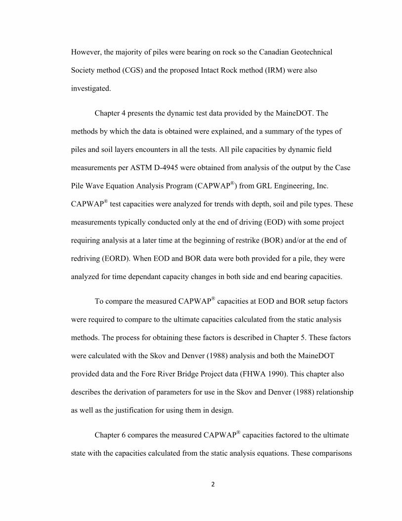
Chapter 4 presents the dynamic test data provided by the MaineDOT. The
methods by which the data is obtained were explained, and a summary of the types of
piles and soil layers encounters in all the tests. All pile capacities by dynamic field
measurements per ASTM D-4945 were obtained from analysis of the output by the Case
Pile Wave Equation Analysis Program (CAPWAP®) from GRL Engineering, Inc.
CAPWAP® test capacities were analyzed for trends with depth, soil and pile types. These
measurements typically conducted only at the end of driving (EOD) with some project
requiring analysis at a later time at the beginning of restrike (BOR) and/or at the end of
redriving (EORD). When EOD and BOR data were both provided for a pile, they were
analyzed for time dependant capacity changes in both side and end bearing capacities.
To compare the measured CAPWAP® capacities at EOD and BOR setup factors
were required to compare to the ultimate capacities calculated from the static analysis
methods. The process for obtaining these factors is described in Chapter 5. These factors
were calculated with the Skov and Denver (1988) analysis and both the MaineDOT
provided data and the Fore River Bridge Project data (FHWA 1990). This chapter also
describes the derivation of parameters for use in the Skov and Denver (1988) relationship
as well as the justification for using them in design.
Chapter 6 compares the measured CAPWAP® capacities factored to the ultimate
state with the capacities calculated from the static analysis equations. These comparisons

3
were conducted for each combination of side capacity methods as well as each of the end
bearing methods. The comparisons were then analyzed for outliers to see if there was
cause for removal. The final comparisons of the methods were conducted using the data
with the justified outliers removed. This chapter also discusses the cause of the scatter in
the data.
The final two chapters of this report summarize the research and provide the
recommended predictions respectively. The recommendations include the best predictive
methods for side capacity, end bearing on rock and end bearing in till. Additionally,
recommendations for obtaining soil strength parameters and dynamic pile measurements
are presented in Chapter 8.
4
Chapter 2:
OVERVIEW OF PILE LOAD TESTING
2.1. Static Load Testing
Static test piles are commonly loaded to twice the design load or failure. Loading
is commonly applied with a jack against a supported weight or against a cross beam
attached to anchor piles. The pile is then unloaded incrementally. The increment of
loading and monitoring time and procedure depend upon the type of load test. Hannigan
et al (2006b) recommends the quick load test method of ASTM D1143, “Standard Test
Method for Piles Under Static Axial Load.” AASHTO (2002) recommends that the
design capacity be evaluated by the Davisson criteria (Davisson 1972). This criterion
defines the pile failure to occur at the intersection of the pile top displacement and a line
offset to the elastic deformation portion of the pile loading. This line is described by the
following equation (Bradshaw and Baxter 2006):
!! =!"!" + (0.15+ 0.008!) [2.1]
Where:
dT = displacement of the top of the pile (inches)
Q = applied test load (lbs)
E = modulus of elasticity of the pile (psi)
A = cross sectional area of the pile (in2)
L = length of the pile (inches)
D = diameter of the pile (inches)

5
The high cost of testing is the main deterrent to static load testing. It also does not
provide information on the quality of the installation or driving efficiency (Bradshaw and
Baxter 2006).
2.2. Dynamic Load Testing
High strain dynamic load testing as specified in ASTM D-4945 is a more cost
effective option to static load testing, and it does verify proper installation. The test can
be administered at any point during the installation, so the pile can be tested if there is
suspected damage or misalignment during driving. The test is also helpful in deciding if
the appropriate hammer is being used for the driving, and if the fuel setting and hammer
stroke are appropriate. The high strain dynamic load tests in this study use the Pile
Driving Analyzer (PDA®) from Pile Dynamics, Inc. (PDI) to collect data during striking,
and the data is refined using a computer program, such as the CAPWAP® of Pile
Dynamics, Inc (PDI), to estimate in situ capacities. The CAPWAP® software conducts a
post-driving numerical evaluation of the raw field data obtained from the dynamic pile
test. High strain dynamic test methods as available with PDI’s PDA® equipment were
used in all the tests covered by this report, so PDA® tests will be referenced.
2.3. Limitations of CAPWAP® Analyses
The study by Lai and Kou (1994) investigated the reliability of using PDA® and
CAPWAP® predictions to validate in situ pile capacities. They concluded that the
CAPWAP® predicted capacities are more reliable than the PDA® predictions alone
because the CAPWAP® analysis refines the Smith damping factor used in the predictions.
However, when the CAPWAP® predictions were compared to a static capacity analysis
using Davisson failure criteria, it was observed that the CAPWAP® analysis could over

6
predicted the static capacity by up to a factor of 1.15. Additionally, it was observed that
CAPWAP® analysis compared to static testing could under predict by a factor down to
0.4 from hammer limitations or from soil disturbance.
Long et al (1999) investigated the effectiveness of dynamic measurements at
predicting the measured static capacity determined using the Davisson criteria. The paper
compared the Engineering News, Gates, WEAP, Measured Energy, PDA®, and
CAPWAP® methods by calculating the wasted capacity index (WCI) for each method.
The WCI is an indication of the uncertainty associated with each method, and it
essentially compares the amount of addition capacity required to ensure that the pile
meets a certain level of certainty. A lower WCI is an indication of a better prediction. The
comparison in this paper was for a 99% reliability of prediction, and the WCI values
reflect this reliability. The results of this study showed that when using the CAPWAP®
analysis at the end of driving (EOD) (WCI = 4.4) it performed the second worst to the
Engineering News method (WCI=5.7). The best method at EOD was the Gates formula
(WCI = 2.1). However, the same comparisons at the beginning of restrike (BOR)
indicated that the CAPWAP® method had a reduction in WCI by a factor 2.4. This
indicated that the CAPWAP® analysis with BOR data had the most reliable predictions
(WCI = 1.8); however, the time at which the BOR tests were conducted was not reported.
7
Chapter 3:
METHODS
In order to estimate the capacities of the piles included in the database the
properties and strength parameters of the soil must first be determined. The Nordlund
method is recommended by the Federal Highway Administration (Hannigan et al, 2006a)
for calculating the capacities of piles driven through granular soils. However, this method
does not provide a limiting value for side capacity and can provide erratic estimates for
piles driven to great depths or through very dense soils.
The FHWA lists both the α-method and the β-method as acceptable methods for
determining the ultimate skin friction of piles driven through cohesive materials.
However, most of the piles included in this study were only tested at end of driving
(EOD) with testing at the beginning of restrike (BOR) for some, so most measured
capacities will be for the cohesive soils in a remolded state. The strength gain with time
(setup) will be applied to measured capacities for comparison to both the undrained α-
method calculation and the drained β-method calculation.
The method currently used by MaineDOT designers for determining the end
capacity in bedrock was developed by the Canadian Geotechnical Society (CGS) in 1985.
This method requires information about the rock quality and the fracture planes contained
within to make an estimate of the end bearing capacity. Typical rock sampling for the
bridge projects does not go further than providing basic information collected from
boring logs. They do not include much (if any) information about the fractures. This
causes the engineer to have to estimate the parameters, which results in inaccurate
estimates of the end capacity. More extensive sampling of the bedrock would be needed

8
for the design equations to perform properly. The following sections detail the methods
used to determine these parameters for granular and cohesive soils, till and bedrock.
3.1. Obtaining Strength Parameters for Granular Soils
The boring logs provided in the geotechnical report for each project provided
standard penetration test (SPT) numbers as the strength parameter for granular soils.
These values were averaged over the designated layers to obtain a representative strength
value. The SPT numbers were corrected for field conditions and effective overburden
pressure using Equation 3.1 (Das 2010).
(!1)!" =!!!!!!!!!
60 ×!! [3.1]
Where:
N = standard penetration test (SPT) number in field
ηH = hammer efficiency (%)
ηB = correction for borehole diameter
ηS = sampler correction
ηR = rod length correction
CN = correction factor
The correction factor (CN) was calculated using the relationship proposed by Liao and Whitman
(1986). This relationship is shown in Equation 3.2.
!! =1
!′! !!
!.!
[3.2]
Where:

9
σ’v = vertical effective stress (psf)
pa = atmospheric pressure (2000 psf)
The relative density (Dr) and Unified Soil Classification System description of the
soil were used to aid in estimating the effective friction angle, dry density, and void ratio
of the soil. The Naval Facilities Engineering Command (1986) published a design chart
for determining these parameters and is shown in Figure 3-1.
Figure 3-1: Granular Soil Strength Parameters (from NavFAC 1986)

10
The relative density (Dr) of the soil for use in Figure 3-1 was correlated from the
field corrected SPT (N60) using the relationship proposed by Meyerhof (1957). This
relationship is shown below.
!! =!!"
17+ 24 !′!!!
!.!
[3.3]
Where:
N60 = field corrected standard penetration test (SPT) number
The total unit weight (γT) and water content of the soil were not always
specifically quantified in the project documents. In the cases where water content was not
available a representative value was obtained from the following relationship.
! =!"!!
[3.4]
Where:
S = degree of saturation
e = void ratio
Gs= specific gravity of the solids
In this calculation due to a lack of information the degree of saturation was
assumed to be 1.0 (saturated) and the specific gravity of the soil solids was assumed to be
2.68 to stay consistent with the assumptions in Figure 3-1 (NavFAC 1986). The void
ratio was obtained from Figure 3-1. After determining the water content of the soil, the
total unit weight (γT) of the layer could be determined from the following equation.

11
!! = !! 1+ ! [3.5]
Where:
γD = dry unit weight
The dry unit weight of the soil is determined from the correlation presented in Figure 3-1.
3.2. Obtaining Strength Parameters for Cohesive Soils
The unit weights (γT) of the cohesive layers were determined based on the
average in situ water content for the soil layer. The following relationships from Holtz
and Kovacs (1981) were used to determine an appropriate value.
! =!×!!! [3.6]
Where:
w = water content
Gs = specific gravity of solids
S = saturation percentage
!! = !! !!1+ !1+ ! [3.7]
Where:
Gs = specific gravity of solids
γw = unit weight of water
w = water content
e = void ratio
To obtain the total unit weight of the cohesive soil, the void ratio of the layer
needed to be determined. Equation 3.6 was used to determine the void ratio (e) by

12
assuming the specific gravity of solids was 2.75 and the saturation percentage (S) was
100%. Equation 3.7 was then used to evaluate the total soil density. The unit weights
determined from this procedure were used in calculations of skin friction of clay layers
using the β-method.
The undrained shear strengths of the soils for both the undisturbed and remolded
soil states were obtained from the geotechnical reports and boring logs where applicable.
The values used in calculations were taken as the average strength for the layer.
However, the undrained shear strengths were not always available from the project
documents. In the cases when the measured undrained shear strengths were not available
representative values were estimated through correlations with the field corrected STP
number (N60). These correlations were provided by Terzaghi, Peck, and Mesri (1996) and
are shown in Table 3-1. The undrained shear strength used in calculations was linearly
interpolated from the ranges provided in the table. The strength valuations in parentheses
are those used by MaineDOT and are 4.4% more conservative than those used in the
calculations.
Table 3-1: Correlations of N60 to Undrained Shear Strength (Terzaghi et al,1996)
Soil Description Very Soft Soft Medium Stiff Very Stiff Hard
N60 <2 2-4 5-8 9-15 16-30 >30
Su (psf)
<261
(<250)
261-522
(250-500)
522-1044
(500-1000)
1044-2089
(1000-2000)
2089-4177
(2000-4000)
>4177
(>4000)

13
3.3. Determination of Side Capacities
The side capacity of each pile was determined by calculating the shear resistance
along the pile in each of the subsurface soil layers as defined in the preceding database.
The side capacity is then taken as the sum of the resistances in each soil layer. The
following sections will describe the methods for calculating the capacities in granular and
cohesive soils. In granular soils The Nordlund method (Hannigan et al 2006), Meyerhof’s
Standard Penetration Test (SPT) method (Hannigan et al 2006), and Meyerhof’s method
(Meyerhof 1976) were considered. In cohesive soils the α-method (Hannigan et al 2006)
and β-method (Hannigan et al 2006) were considered.
3.3.1. Nordlund Method for Granular Soils
The Nordlund method (Nordlund 1963) is useful for cohesionless soils of sand
size or smaller. The first step in this method is to determine the friction angle of the soil
against the pile (δ) for the layer being analyzed. Nordlund provided ratios of soil-pile
friction angle to soil friction angle (ϕ) as shown in Figure 3-2.

14
Figure 3-2: Friction Angle at Soil Pile Interface (after AASHTO 2010)
This ratio is obtained by entering the figure with the volume of displaced soil and
in situ friction angle and finding the curve related to the correct pile type. The volume of
displaced soil is quantified by cubic feet of soil displaced per linear foot of driving. This
is effectively the cross-sectional area of the pile. Nordlund provided curves for H-piles
and closed end pipe piles, but did not provide one for open end pipe piles. To cope with
this issue, it was assumed that there would be some plugging to some extent within the
pile that would provide a closed end condition and the closed end curve could be used.
After the ratio is pulled from the figure, it is multiplied by the in situ soil friction angle to
obtain the soil-pile friction angle.
Table 3-2 presents the design values for the lateral earth pressure coefficient (Kδ)
for use in Equation 3.8. The values are determined from the amount of soil displaced by
0.0
0.5
1.0
1.5
2.0
2.5
3.0
3.5
4.0
0.00 0.25 0.50 0.75 1.00 1.25
Displaced Soil Vo
lume (cu. 2/2
)
δ/φf
H-‐Piles
Closed Ended Pipe
15
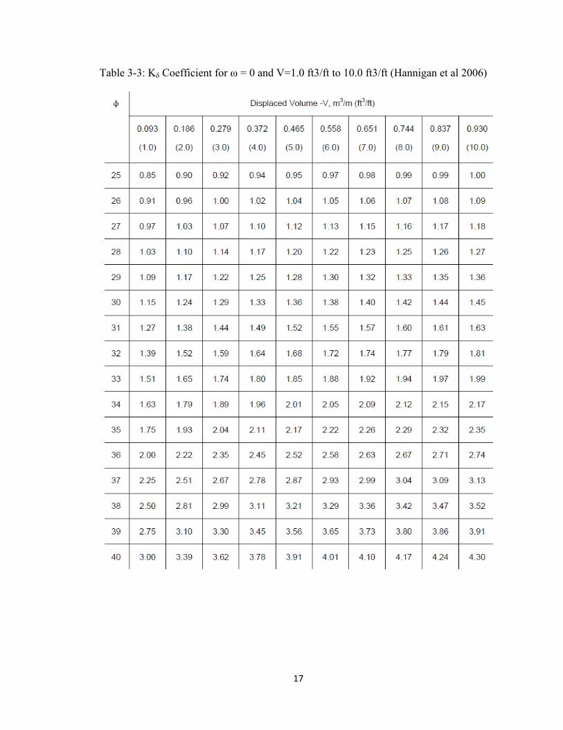
the pile and the friction angle of the soil. Hannigan et al (2006) recommends that a linear
interpolation be used to find values that fall between the rows of the table, and log linear
interpolation is used to obtain values that fall between the columns. The values displayed
in the table are for piles with no taper, such as the piles included as a part of this
database. The volume of soil displaced by the pile can then be used along with the failure
angle of the soil and the pile type to find the soil-pile friction angle.
If it is determined that the soil-pile friction angle differs from the failure angle in
the soil, a correction factor (CF) needs to be factored into the capacity calculation. The
factor is used to correct the Kδ value, and can be obtained from Figure 3-3.

16
Table 3-2: Kδ Coefficient for ω = 0 and V=0.1 ft3/ft to 1.0 ft3/ft (Hannigan et al 2006)
17
Table 3-3: Kδ Coefficient for ω = 0 and V=1.0 ft3/ft to 10.0 ft3/ft (Hannigan et al 2006)

18
Figure 3-3: Correction Factor for Lateral Earth Pressure Factor (Hannigan et al 2006)
Once all of the parameters have been determined, the side capacity can be
estimated using the equation provided below:
!! = !!!!! ′!sin ! + !cos! [3.8]
Where:
σ’v = vertical effective stress (ksf)
ω = pile taper (equal to 0 for all piles in this study)
Equation 3.8 calculates the unit skin resistance of the pile in a granular soil layer.
To obtain the total capacity of the pile, the unit resistance must be multiplied by the
surface area of the pile. The surface area is calculated as the product of the pile perimeter
and the embedded length of the pile in the layer. For H-piles a box perimeter was

19
assumed. For displacement needed in Figure 3-2, Table 3-2, and Table 3-3, the steel
cross-sectional area is used. The Nordlund method does not use a limiting shear stress
after a given depth.
Nordlund’s method creates some problems without a limiting value for
overburden stress with depth. In a report published by the FHWA (1990), static pile
capacity estimates were compared to the results of static and dynamic load testing in
Portland, Maine. The study was conducted on the Fore River Bridge replacement which
connects Portland to South Portland. The subsurface profile on the project is shown in
Figure 3-4. It shows that there is a significant amount of granular material on the site with
significant amounts of till encountered in Boring B17 & B23.
Figure 3-4: Soils at Fore River Bridge (FHWA 1990)

20
After the piles were installed, some piles were tested dynamically at EOD and
BOR and 4 piles were tested with a static load test. The results of the testing as well as
the Nordlund predicted capacity are shown in Table 3-4. The limitations of Nordlund’s
method are easily visible upon analysis of the test results. It proves to be under-
conservative for all piles except for the HP 14x117 piles. In some cases it over predicted
the measured pile capacities by over 300 tons.
Table 3-4: Predicted to Measured Pile Capacities at Fore River Bridge (FHWA 1990)
Nordlund CAPWAP® Static Load Test
Pile Length (ft) (kips) EOD
(kips) BOR (kips)
Restrike Time (days) (kips)
18" C.E.P 79.1 610 336 414 1 N/A 18" C.E.P 99.9 858 346 500 2 440 18" C.E.P 71.3 1040 424 526 1 400 18" C.E.P 50.8 720 N/A N/A N/A N/A 18" C.E.P 71.1 1040 416 436 3 N/A 18" C.E.P 50.8 720 322 340 6 350 HP 14x89 131.0 806 564 286 3 N/A HP 14x89 114.7 806 N/A 238 N/A N/A HP 14x89 115.0 1476 278 328 5 N/A HP 14x89 114.7 1476 296 306 5 N/A HP 14x117 135.5 966 732 1104 8 900 (Did Not Fail) HP 14x117 133.8 966 1010 770 1 N/A
3.3.2. Standard Penetration Test (SPT) Based Method for Granular Soils
In 1976 Meyerhof proposed a method for correlating the side capacity of pile in
granular soils to the standard penetration test (SPT). Hannigan et al (2006) built off of his
research and suggest that the side capacity of the pile is directly proportional to the

21
modified SPT readings, however, the equation changes slightly for high displacement and
low displacement piles. The equation for both scenarios is detailed below:
!! = !(!!)!" ≤ 2!"# [3.9]
Where:
(N1)60 = average corrected SPT value for the layer for overburden pressure
C = constant, equals 1/25 for displacement piles, equals 1/50 for low
displacement piles
To obtain the total capacity of the pile the unit resistance must be multiplied by
the surface area of the pile. The surface area is calculated as the product of the pile
perimeter and the embedded length of the pile in the layer. For H-piles a box perimeter
was assumed.
3.3.3. Meyerhof Method for Granular Soils
Meyerhof proposed another method in 1976 that was based on soil strength
parameters. This method related the unit shaft resistance to the horizontal effective stress
(σ΄h) to the soil-pile friction angle (δ). NavFAC (1986) suggested δ value of 20° for steel
piles was used in the calculation. The σ΄h is related to the vertical effective stress (σ΄v) by
an effective earth pressure coefficient (Kh). The proposed equation is shown below in
Equation 3.10.
!! = !!!!! tan ! [3.10]

22
The Kh value was estimated based on recommendations by NavFAC (1986). They
recommend that for a single driven steel H-pile a Kh value between 0.5-1.0 and for a
single displacement pile Kh values between 1.0-1.5. It was desired to relate Kh to the
coefficient of earth pressure at rest (Ko). The Ko value was determined from the
relationships found by Kulhawy and Mayne (1990) shown in Figure 3-5.
The friction angles used in the figure were determined as described in Section 3.1.
However, for the friction angles of till this method may lead to unrealistic values since
there is a substantial amount of fines. To address this, a limiting value of 38° was used as
measured by Linell and Shea (1960) for New England tills.
Figure 3-5: Relationship Between OCR and Ko (Kulhawy and Mayne 1990)
The benefit of using the Meyerhof method is that there is a limiting stress with
depth that is applied to the calculation to prevent erratic values with depth. Sowers (1979)

23
using Vesic (1967) recommends that for Dr>70% the effective overburden stress should
be calculated to be constant for a depth greater than 20 times the pile diameter and for
Dr<30% the effective overburden stress should be calculated to be constant for a depth
greater than 10 times the pile diameter. These depths are referred to as critical depths
(L΄), and were determined for homogenous sands. However, the soil layers are often not
homogeneous along the length of the pile. In the cases where the soil layers above L΄ did
not have a homogeneous Dr, L΄ was calculated as 15 times the pile diameter. To obtain
the total capacity of the pile the unit resistance must be multiplied by the surface area of
the pile. The surface area is calculated as the product of the pile perimeter and the
embedded length of the pile in the layer. For H-piles a box perimeter was assumed.
3.3.4. Meyerhof Method Adjustments for Basal Till Layers
Basal till is extremely dense as it was deposited beneath continental glaciers with
a thickness of more than a mile. Since the glaciers subsequently melted, the basal till
deposits are highly consolidated with a corresponding high K value. Meyerhof’s method
was derived for sands as described previously, so some K correction factor is needed to
account for basal till’s overconsolidated state.
The passive earth pressure of the soil is the maximum pressure that can be exerted
on to the soil. By calculating the passive pressure coefficient, the limiting value for
horizontal earth pressure coefficient (Kh) will be known. This passive pressure coefficient
is well under the K resulting from the removal of more than one mile depth of ice
overburden. The passive pressure coefficient (Kp) was calculated using the method
outlined by NavFAC 7.02 (1986). The design chart for this method is shown in Figure
3-6. The friction angle for till was taken to be 38° for the reasons described previously.

24
Figure 3-6: Passive Pressure Coefficient Determination (NavFAC 1986)
25
For a horizontal soil surface with β equal to 0°, the Kp is equal to 14.0. For planar
failure with release of overburden ice pressure, it is equivalent to the friction angle
between the soil and the wall (δ) being 0°. A reduction factor (R) of 0.302 is applied to
Kp resulting in an adjusted Kp of 4.2. Alternatively, this describes the Rankine passive
condition where:
!! = tan! 45+ ! 2 [3.11]
For a ϕ = 38°, Kp= 4.20 by this equation.
Using a K=4.2 for a displacement pile in basal till, it would be anticipated that an
H-Pile will have a lower K. The same ratio of K (0.75/1.25) is maintained in the basal till
as in the normally consolidated granular material. This gives a working ! = 4.2× !.!"!.!"
=
2.52 (call 2.5) for the H-pile.
3.3.5. α – Method for Cohesive Soils
The α-method (Tomlinson 1957) for pile support in cohesive soils uses the
undrained strength of the clay to obtain capacity. This method presumes that an
undrained failure is the critical shear for piles in cohesive material. The American
Association of State Highway and Transportation Officials’ (AASHTO) LRFD Bridge
Design Specifications (2010) provides the α-method as one method for determining the
side capacity of piles through various cohesive soil materials. In the α-method, the
adhesion at the pile-soil interface is formed by applying a factor to the undrained shear
strength. The side capacity is the summation of the adhesion over the perimeter area of
the sides of the pile. The α-method is described below:

26
!! = !!! [3.12]
Where:
α = adhesion factor determined from design charts
Su = undrained shear strength (ksf)
The design charts below provide the α adhesion factors to use for clays overlain
by different soil types. The α factors are determined by entering the design charts with
the undrained shear strength and depth of embedment into the layer to pile width ratio.
The undrained shear strengths and remolded undrained shear strengths are determined
through the methods described in Section 3.2. The ultimate resistance for the clay layer is
calculated using the adhesion determined from the undisturbed undrained shear strength
and the corresponding α factor. The adhesion resistance at EOD, which is representative
of most the piles included in this study, is calculated using the remolded undrained shear
strengths and the corresponding α factor. To obtain the total capacity of the pile the
adhesion resistance must be multiplied by the surface area of the pile. The surface area is
calculated as the product of the pile perimeter and the embedded length of the pile in the
layer. For H-piles a box perimeter was assumed.

27
Figure 3-7: Adhesion Factors for The α – Method (Hannigan et al 2006)
3.3.6. β – Method For Cohesive Soils
The β-method is an effective stress method for cohesive soil. This method
presumes that the critical failure will be a drained failure. This β-method for cohesive
soils is similar to the Meyerhof method for granular soils. However, it combines the

28
Khtan(δ) term of the Meyerhof method into a single factor, β. This method estimates side
capacity by finding the side shear with a directly proportionate relationship to vertical
effective stress. The vertical effective stress is multiplied by a factor that represents the
ratio of the soil’s shear strength to vertical effective stress. The equation for the β-method
is shown below (Hannigan et al 2006):
q! = βσ′! [3.13]
Where:
β = a factor determined from Figure 3-8
σ’v = vertical effective stress (ksf)
The FHWA recommended method for finding the β factor is shown in Figure 3-8.
They have correlated the β factor to the effective drained friction angle and soil type.
However, the drained friction angle for cohesive materials is rarely measured in practice.
To circumvent this, a typical friction angle was assumed for the entire Presumpscot
Formation. Sandford and Amos (1987) reported an effective friction angle of 35° for the
Presumpscot Formation in a 1987 report on a landslide in Gorham, Maine. This value
was used to obtain a β factor. The β method gives strengths after all pore pressures from
driving have dissipated. To obtain the total capacity of the pile at EOD the unit resistance
at EOD must be multiplied by the surface area of the pile. For the full capacity of the pile
after dissipation, the strength with full setup is used. The surface area is calculated as the
product of the pile perimeter and the embedded length of the pile in the layer. For H-piles
a box perimeter was assumed.

29
Figure 3-8: β Factor Determination (Hannigan et al 2006)
3.4. End Bearing on Bedrock
End bearing capacity in rock can be difficult to determine. These values are not
necessary for all types of piles because some piles, especially concrete, will fail in
compression before the bedrock. In most applications in Maine steel piles are used, so the
end bearing on rock becomes relevant. Typical capacity values for different bedrock
materials can be found in literature; however, it is intuitive that these values will not
provide reliable values for every site. Bedrock can be weathered, highly fractured, or
more poorly formed than anticipated from the literature. To get an idea of the type and
quality of rock at a project site the borings should sample past refusal and collect some
bedrock. There are two different methods that were studied to determine the bearing
capacity of bedrock. However, first the cross sectional area of the piles must be adjusted
for pile tip protectors which increase the bearing area of the pile on bedrock.

30
To find the pile tip area the dimensions of the protective driving shoe needed to
be obtained. MaineDOT (Krusinski 2012) reported that the two typical H-pile driving tips
used on bridge projects in the State are the APF HP 77600-B and the APF HP 77750-B.
The dimensions on these pile tips were found on the R.W. Conklin Steel Supply website,
and are shown in Appendix A. A request for information submitted to Associated Pile &
Fitting (2012) provided tip protection dimensions for both conical (for closed end pipe
piles) and cutting shoe (for open end pipe piles). The dimensioned drawings they
provided can be found in Appendix A.
3.4.1. Canadian Geotechnical Society Method For End Bearing in Rock
In 1985 the Canadian Geotechnical Society (CGS) proposed a method in which
bearing capacity is determined from measurements of the fractures in the bedrock. The
method is described in the following equation (Turner 2006):
!!"# = 3!!3+ !!!
10 1+ 300 !!!!
1+ 0.4!!!
[3.14]
Where:
qu = unconfined compressive strength of bedrock
sv = vertical distance between fractures
td = thickness of fracture
B = diameter of boring in bedrock
Ls = depth of penetration into bedrock
The unconfined compressive strengths (qu) were obtained from the geotechnical
reports for each project. The MaineDOT rarely perform unconfined compression testing

31
on bridge projects and assume qu from correlations provided in AASHTO Standard
Specifications for Highway Bridges 17th ed. (2002). In the cases where qu was
unavailable from the reports a value was assumed based on the rock type and qu for those
rock types on similar projects. When the calculations for the CGS method were provided
in the geotechnical design reports, they were used in this study. However, for projects
that did not include the calculation a procedure was needed to evaluate the input
parameters without the bedrock samples.
The piles installed on the bridge projects included in this study were rarely
socketed into bedrock, so the depth of penetration into bedrock (Ls) was set equal to zero.
Although there was no specified driving of the pile into bedrock, the equation would not
function properly if B was set equal to zero. Therefore B was set to 1 foot (approximate
width of the piles) for calculations. The thickness of fractures (td) in the bedrock and the
vertical spacing between fractures (sv) were interpreted from the bedrock descriptions in
the boring logs. The boring logs provide bedrock core descriptions including rock type,
dip, spacing, tightness and infilling of the discontinuities. MaineDOT (Krusinski 2012)
indicated that from the rock samples examined, the sv can range from inches to feet and
the fractures range from 1/64-inch for tight joints/bedding to <1/4 for open/healed joints.
To determine the total capacity, the value calculated in the CGS method must be
multiplied by the cross sectional area of the pile on bedrock.
3.4.2. Proposed Intact Rock Method For End Bearing
The proposed Intact Rock Method (IRM) for end bearing is equivalent to the
Rowe and Armitage (1987) equation (cited by Turner, 2006) that relates the ultimate
32
bearing capacity of intact rock to the compressive strength of the bedrock. The equation
is presented below:
!! = 2.5!! [3.15]
Where:
qp = end bearing capacity of the bedrock
qu = unconfined compressive strength of the bedrock
3.5. Tip Capacity for Piles Bearing in Till
There are a few piles included in the study that were designed to obtain support
from soils without bearing on bedrock. There are also some piles that fetched up in the
till or other overlying strata. There were not any piles that experienced end bearing in
cohesive strata, so tip capacity in cohesive soils will not be considered in this report. The
methods for determining end bearing on piles above bedrock are described in this section.
3.5.1. Nordlund Method
The Nordlund method (Nordlund 1963) comprised a bearing capacity relation
from Berezantzes et al (1961) which did not have a limiting value. Since the Nordlund
(1963) paper, the bearing capacity relation has been changed and a limiting value from
Meyerhof (1976) has been added by Hannigan et al (2006a) based on Bowles (1977).
Subsequent editions (Bowles 1982; Bowles 1988) do not use this method. The end
bearing capacity of the soil now associated with the Nordlund method is detailed below
(Hannigan et al, 2006a):
!! = !!! ′!! ′! ≤ !! [3.16]
Where:
αt = coefficient determined from Figure 3-9.
33
N’q = bearing capacity factor determined from Figure 3-10.
σ’v = vertical effective stress (ksf)
qL = maximum end bearing (ksf) from Figure 3-11 (Meyerhof 1976).
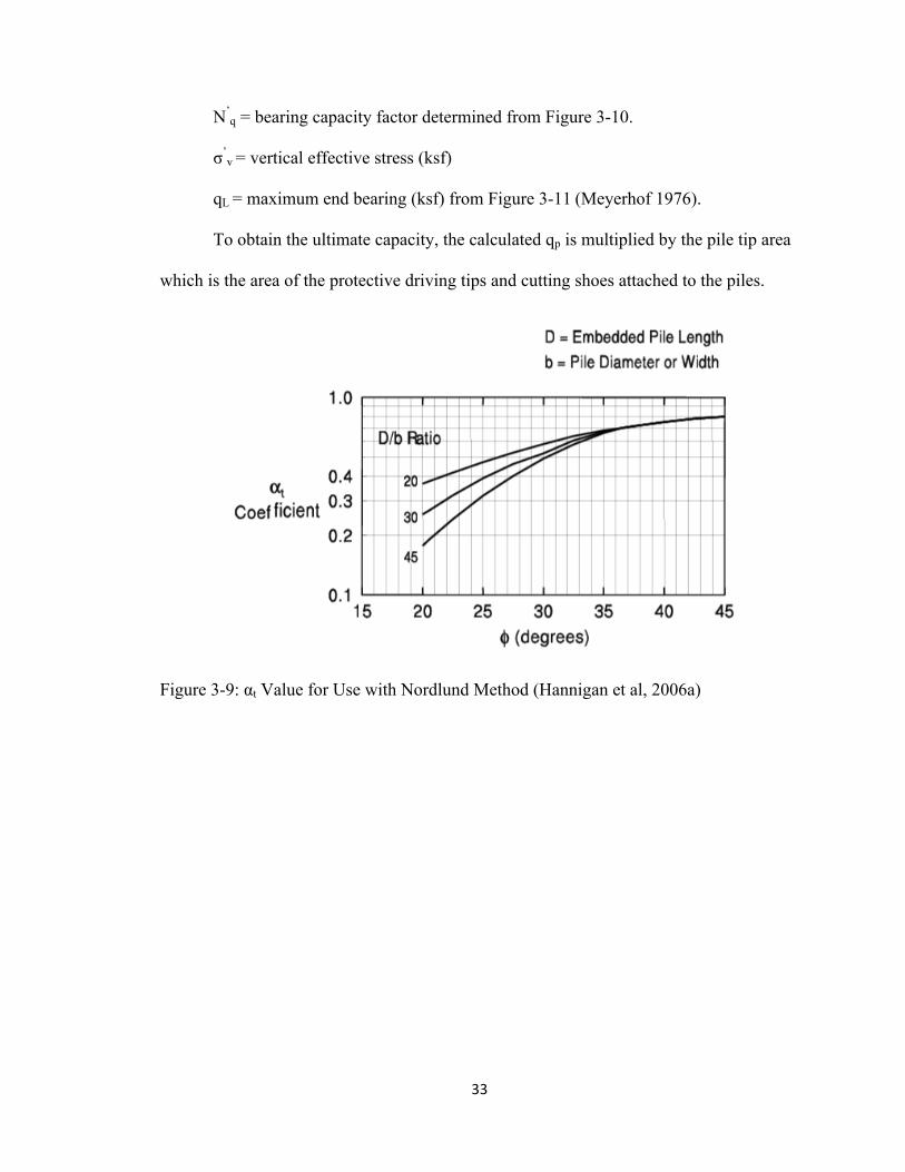
To obtain the ultimate capacity, the calculated qp is multiplied by the pile tip area
which is the area of the protective driving tips and cutting shoes attached to the piles.
Figure 3-9: αt Value for Use with Nordlund Method (Hannigan et al, 2006a)

34
Figure 3-10: Bearing Capacity Factor for Use with Nordlund Method (Hannigan et al,
2006a)
Figure 3-11: Ultimate Unit Base Capacity Based on Soil Friction Angle (Hannigan et al,
2006a)

35
3.5.2. Meyerhof Standard Penetration Test (SPT) Method
The Standard Penetration Test Method (SPT) method proposed by Meyerhof
(1976) is another method for determining the bearing capacity of piles in cohesionless
soils. It uses SPT and modified SPT values to determine the capacity values. The end
bearing capacity is determined using the following equation:
!! =0.8× !! !"×!
! ≤ !! [3.17]
Where:
(N1)60 = corrected SPT value of the bearing strata
D = driven depth of pile (feet)
d = pile diameter (feet)
qL = maximum end bearing from design tables (ksf)
The maximum end bearing value (qL) for this equation is eight times the modified
SPT value (8(N1)60) for sands (AASHTO 2010). To obtain the ultimate capacity, the
calculated qp is multiplied by the pile tip area which is the area of the protective driving
tips and cutting shoes attached to the piles.
3.5.3. Meyerhof Method
The Meyerhof method (1976) for determining point capacity uses a generalized
formula that relates the pile capacity to the overburden pressure and self weight of the
soil at the pile tip. This method is not specified in AASHTO (2010), but the limiting
value for the Nordlund method in AASHTO (10) has been derived from the Meyerhof
method. For piles with lengths beyond about 15 ft, the limiting value typically controls
the capacity. In the full formula the cohesion at the tip is considered, however, none of
36
the pile tips were located in a cohesive bearing stratum. Ignoring the cohesive term, pile
tip capacity is calculated as:
Q! = A!σ!!N! ≤ !!!! [3.18]
Where:
Nq = bearing capacity factors
σv' = overburden stress at pile tip (ksf)
Ap = cross sectional area of pile tip (ft2)
!! = limiting bearing stress (ksf) = 0.5paNqtanø
pa = atmospheric pressure (2.0 ksf)
The bearing capacity factor (Nq) is taken from design charts from Meyerhof
(1976). Nq΄ is determined using the friction angle of the soil in the bearing stratum, the
length to width ratio of the pile, and the Nq΄ curve from Figure 3-12.
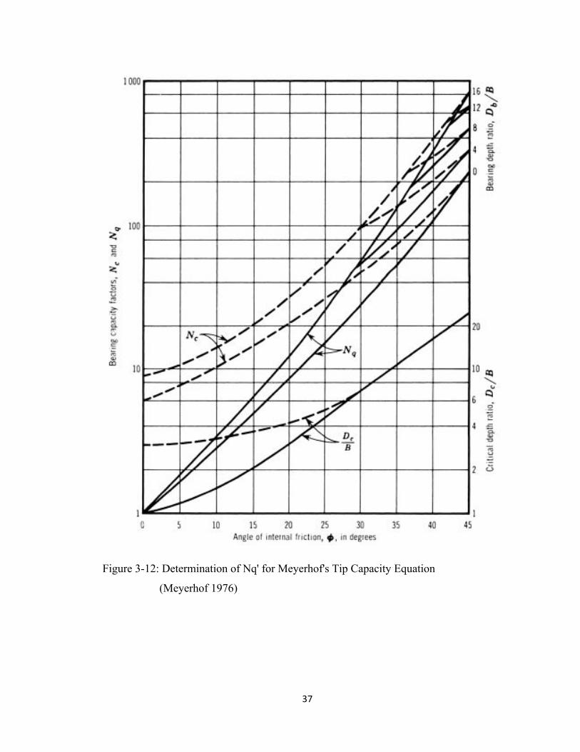
37
Figure 3-12: Determination of Nq' for Meyerhof's Tip Capacity Equation
(Meyerhof 1976)

38
Chapter 4:
DESCRIPTION OF AVAILABLE DATA
4.1. Process of Test Data Collection
The MaineDOT uses the dynamic pile load test following the procedures in
ASTM D-4945 to determine the in situ capacity for piles installed on bridge projects in
the State. In this method, pile driving waves generated by the blow of a pile driving
hammer are monitored in the field. These dynamic field measurements are entered to a
pile-soil software model that yields an estimate of pile side and end capacity at the
moment of the hammer blows. The Pile Dynamic Inc. (PDI) software, PDA® and
CAPWAP® are routinely employed by pile testing subcontractors on MaineDOT projects.
Typically one pile from each group was selected as a representative of the group
to test its capacity. The piles are normally tested at the end of driving (EOD). Sometimes
piles are subjected to additional load testing at a later time to assess the time dependent
change of pile capacity. Pile capacity information from dynamic testing was provided
with the project documents and was used to gauge the effectiveness of the capacity
estimates provided by design methods.
Pore pressures generated during pile driving affect the capacity measured at the
EOD. Capacities in clay at the EOD can be significantly less than capacities measured
after pore pressure dissipation, while capacities in granular soils are less affected with
time. Thus CAPWAP® estimates of capacity at EOD generally underestimate the long
term capacity.

39
4.2. Descriptions of Test Piles and Soil Profiles
4.2.1. General
The data provided by MaineDOT included the majority of the dynamic tests
conducted from the fall of 1994 through the spring of 2012. During this period, there
were 80 different bridge projects with 258 piles selected for dynamic capacity testing
using a high strain dynamic testing per ASTM D4945 withCAPWAP® analyses on
measured field data. Of these piles 90% were end bearing on bedrock while 10% were
bearing in till strata. The data consisted predominantly of low displacement piles (H-piles
and open end pipe piles) with only 11% of all tests being conducted on closed end pipe
piles. A tabulation of the pile types tested is shown in Table 4-1. The side capacities
versus penetration depth were analyzed to look for trends with pile type.
Table 4-1: Distribution of Pile Types Included in Project Data
Type of Pile # of Piles
12" H-‐piles 24 14" H-‐piles 158 30" Pipe Open 2 26" Pipe Open 3 24" Pipe Open 23 22" Pipe Open 17 20" Pipe Open 1 30" Pipe Closed 2 26" Pipe Closed 1 24" Pipe Closed 19 20" Pipe Closed 8 Total # of piles 258
40
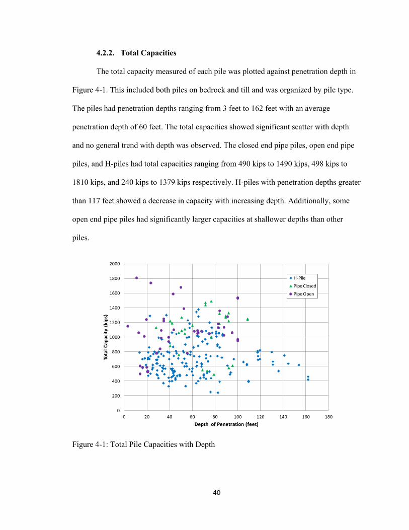
4.2.2. Total Capacities
The total capacity measured of each pile was plotted against penetration depth in
Figure 4-1. This included both piles on bedrock and till and was organized by pile type.
The piles had penetration depths ranging from 3 feet to 162 feet with an average
penetration depth of 60 feet. The total capacities showed significant scatter with depth
and no general trend with depth was observed. The closed end pipe piles, open end pipe
piles, and H-piles had total capacities ranging from 490 kips to 1490 kips, 498 kips to
1810 kips, and 240 kips to 1379 kips respectively. H-piles with penetration depths greater
than 117 feet showed a decrease in capacity with increasing depth. Additionally, some
open end pipe piles had significantly larger capacities at shallower depths than other
piles.
0
200
400
600
800
1000
1200
1400
1600
1800
2000
0 20 40 60 80 100 120 140 160 180
Total C
apacity
(kips)
Depth of Penetration (feet)
H-‐Pile
Pipe Closed
Pipe Open
Figure 4-1: Total Pile Capacities with Depth

41
4.2.3. Side Capacities
The piles were also plotted with side capacity versus depth in Figure 4-2. The data
showed that 52% of the pile lengths were driven into cohesive strata. These piles were
then grouped by the percentage of their total lengths penetrating cohesive strata.
• > 0-20% - 40 piles
• 20-40% - 38 piles
• 40-60% - 21 piles
• 60-80% - 20 piles
• 80-100% - 14 piles
These categories of cohesive percentages are helpful in the prediction of behavior
for each pile because clay along the side of the pile lowers the capacity at EOD. The data
indicated that at EOD the piles with lengths 80-100% cohesive had an average side
capacity of 56 kips; lengths 60-80% cohesive had an average side capacity of 78 kips;
and lengths 40-60% cohesive had an average side capacity of 22 kips. The piles with >0-
20% and 20-40% of their total length in cohesive strata had average side capacities of
213 kips and 141 kips respectively.
The side capacities of the piles were observed to generally increase with depth
for piles with less than 40% of its length in cohesive soil. However, the side capacities of
piles with greater than 40% of its length in cohesive soil appear to be more susceptible to
the sensitivity of its cohesive layer(s). There were also a considerable amount of piles
that exhibited lower capacities than their depth of penetration would indicate.

42
Additionally, the data indicated that there were some piles which had side capacities
significantly larger than the majority of the other piles.
Approximately 70% of the 258 piles were driven through a till layer (not
considered cohesive). These piles are grouped below by the percentage of their total
lengths within till strata.
• > 0-20% - 41 piles
• 20-40% - 50 piles
• 40-60% - 42 piles
• 60-80% - 15 piles
• 80-100% - 31 piles
`
0
100
200
300
400
500
600
700
800
900
0 20 40 60 80 100 120 140 160 180
Side
Capacity
(kips)
Length of Pile (feet)
> 0-‐20% Cohesive
20-‐40% Cohesive
40-‐60% Cohesive
60-‐80% Cohesive
80-‐100% Cohesive
100% Granular
Figure 4-2: Side Capacities with Depth

43
4.3. Setup Characteristics of Test Data
Figure 4-3 presents the side and end bearing capacities of piles with both
beginning of restrike (BOR) and EOD test data. The BOR tests were typically tested at
one day after initial drive. The data indicated that approximately 78% of side capacities
increased with time albeit only one day after driving. This time dependent capacity
increase can cause piles to exhibit significantly larger strengths than the measured
capacities at EOD or even one day BOR would indicate. However, the data also indicated
that approximately 70% of the end bearing capacities decreased within the first day after
driving. The figure also had several data points which appear to be abnormal and upon
further inspection it was evident that these data points corresponded to two unique
projects in Canaan and Falmouth.
0
200
400
600
800
1000
1200
1400
1600
0 200 400 600 800 1000 1200 1400 1600
BOR (kips)
EOD (kips)
Side Capacity
End Capacity
Figure 4-3: BOR versus EOD Pile Capacities

44
It was expected that the side capacity would increase with depth, but there were
not any trends by pile type observed. Another observation was that in general the open
end pipe piles had the largest tip capacities in both bedrock and till. This is
counterintuitive to the expectation that the closed end pipe piles would have the largest
pile capacity because they have the largest cross sectional area.
It is expected that the tested piles included in the study will experience time
dependent changes in capacity. However, only 27 piles in this study were tested at EOD
and BOR with each test providing a side and end bearing capacity estimate. Those that
were tested for time dependent changes in capacity are listed in Table 4-3. The table
provides EOD and BOR information for both side and end bearing capacity, the
percentage of clay along the length of the pile, and water content of the clay layer (where
applicable).
Setup values could be determined for the piles close to one day after driving,
since most piles (23) had the restrike BOR the day after the EOD measurement, with 3
piles on the second day and one pile at one hour after the EOD. The first step was to
determine the setup for piles in granular soils. There were 5 piles which had only granular
soils along their entire length. Four of these piles were H-piles which had an average
setup of 1.07; the other pile was a closed end pipe pile which had a setup of 1.51. These
values were then used to back-calculate setup factors for the cohesive layers for piles
driven through mixed soil strata. When combined with the percentage of cohesive and
granular soil along the side of the pile and the overall BOR/EOD ratio, the setup of the
cohesive layers could be determined. On average the raw setup for H-piles was 2.08, for
45
open end pipe piles was 1.92, and for closed end pipe pile 2.31 based on 6, 4, and 3 piles
respectively. In general, these setup values correspond to a time equal to about one day.
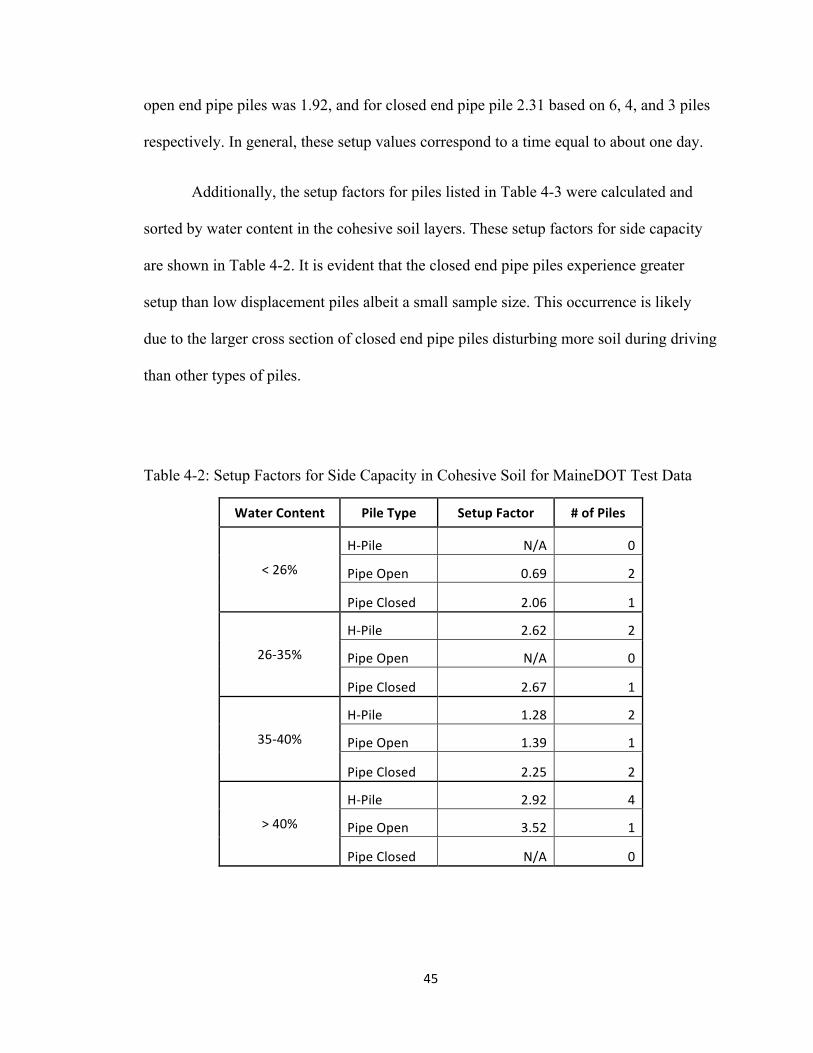
Additionally, the setup factors for piles listed in Table 4-3 were calculated and
sorted by water content in the cohesive soil layers. These setup factors for side capacity
are shown in Table 4-2. It is evident that the closed end pipe piles experience greater
setup than low displacement piles albeit a small sample size. This occurrence is likely
due to the larger cross section of closed end pipe piles disturbing more soil during driving
than other types of piles.
Table 4-2: Setup Factors for Side Capacity in Cohesive Soil for MaineDOT Test Data
Water Content Pile Type Setup Factor # of Piles
< 26%
H-‐Pile N/A 0
Pipe Open 0.69 2
Pipe Closed 2.06 1
26-‐35%
H-‐Pile 2.62 2
Pipe Open N/A 0
Pipe Closed 2.67 1
35-‐40%
H-‐Pile 1.28 2
Pipe Open 1.39 1
Pipe Closed 2.25 2
> 40%
H-‐Pile 2.92 4
Pipe Open 3.52 1
Pipe Closed N/A 0

46
Tabl
e 4-
3: L
ist o
f Pile
s Tes
ted
at E
OD
and
BO
R
w %
N/A
N/A
Unknow
n
N/A
N/A
40.3
42.8
36.6
36.6
40.3
40.3
36.6
42.9
25.2
36 36.4
29.6
22.3
35.5
N/A
24 31.55
32 38.7
38.7
38.7
38.7
% Le
ngth in Clay
0.0
0.0
3.5
0.0
0.0
16.1
47.3
17.6
17.4
38.4
38.3
16.8
89.0
21.6
23.5
77.0
21.5
71.3
26.7
0.0
13.1
14.0
19.5
26.5
19.1
16.0
7.5
BOR
430
769.9
660
737
950
600
270
320
150
270
220
20 690
1130
560
1290
650
880
910
1040
1370
810
475
930
610
440
990
EOD
450
710
726
736
935
760
310
370
170
580
440
60 890
1160
530
1340
770
860
940
1110
900
930
465
1010
760
420
1130
BOR
180
355
362
338
429
280
190
300
240
540
520
220
260
90 10 250
30 210
340
250
120
660
108
120
270
320
100
EOD
210
345
314
312
346
140
110
260
230
210
250
190
80 90 10 190
20 190
300
160
100
510
71 100
460
640
140
BOR # of Days
1/24
2 1 2 2 1 1 1 1 1 1 1 1 1 1 1 1 1 1 1 1 1 1 1 1 1 1
Pile Ty
pe
HP 14x73
Grade 50
HP 14x11
7
HP 14x11
7
HP 14x11
7
HP 14x11
7
HP 14x73
Grade 50
HP 14x73
Grade 50
HP 14x73
Grade 50
HP 14x73
Grade 50
HP 14x73
Grade 50
HP 14x73
Grade 50
HP 14x73
Grade 50
22" P
ipe O
pen
22" P
ipe O
pen
HP 12x53
Grade 50
22" P
ipe O
pen
HP 14x89
Grade 50
22" P
ipe O
pen
20" P
ipe C
losed
20" P
ipe C
losed
20" P
ipe C
losed
24" P
ipe C
losed
HP 14X
89 Grade 50
24" P
ipe C
losed
24" P
ipe C
losed
24" P
ipe C
losed
24" P
ipe C
losed
Pile ID
20 A-‐20
B-‐1
B-‐14
Q-‐15
14 11 27 30 2 9 1 2 3 3 11 6 14 3 2 3 3 4 2 2 3 3
Structure
Abutment 1
Prospect Veron
a Brid
ge
Prospect Veron
a Brid
ge
Prospect Veron
a Brid
ge
Prospect Veron
a Brid
ge
Pier 1
Abutment 2
Pier 2
Pier 2
Pier 3
Pier 3
Abutment 1
Pier 3 W
est
Abutment 1
Pier 1
Pier 1 Ea
st
Pier 3 North
Pier 5 W
est
Pier 1
Pier 3
Pier 4
Pier 5
East Abu
t.
Pier 2
Pier 7
Pier 8
Pier 9
Locatio
n
Norridgew
ock
Verona Islan
d
Verona Islan
d
Verona Islan
d
Verona Islan
d
Falmou
th
Falmou
th
Falmou
th
Falmou
th
Falmou
th
Falmou
th
Falmou
th
Portland
Portland
Portland
Portland
Portland
Portland
York
York
York
York
Canaan
Canaan
Canaan
Canaan
Canaan
Project ID
6900
.00
7965
.00
7965
.00
7965
.00
7965
.00
1509
4.00
1509
4.00
1509
4.00
1509
4.00
1509
4.00
1509
4.00
1509
4.00
1510
6.00
1510
6.00
1510
6.00
1510
6.00
1510
6.00
1510
6.00
1511
0.00
1511
0.00
1511
0.00
1511
0.00
1561
8.00
1561
8.00
1561
8.00
1561
8.00
1561
8.00
End (kips)
Side
(kips)

47
As piles have more end bearing on rock (higher capacities), the end bearing shows
progressively less loss in the first days after driving as shown in Table 4-4 for H-piles.
More than one-half of end bearing restrike capacity data was from H-piles that covered 5
projects. The setup data shows that H-piles lose end capacity for the first days (setup is
0.93) when the end capacity is less than 500 k, where it is expected that most pile ends
are founded on till. For H-pile capacities of 500-800 k, where mostly rock end bearing is
anticipated, there is a slight loss of capacity (setup is 0.97). While for end bearing greater
than 800 k, where it is expected that all piles are founded on rock, there is a slight gain of
H-pile end capacity (setup is 1.02). In contrast to H-piles, pipe piles with closed end for
capacities greater than 800 k show a drop in capacity (setup is 0.91), while open pipes
having a greater than 800 k end capacity have a between setup of 0.94.
Table 4-4: End Bearing Setup Factors for MaineDOT Test Data
End Bearing Capacity Pile Type Setup
Factor # of Piles
< 500 kips H-‐Pile 0.93 6 Pipe Open N/A 0 Pipe Closed 1.05 1
500-‐800 kips H-‐Pile 0.97 5 Pipe Open N/A 0 Pipe Closed 0.80 1
> 800 kips H-‐Pile 1.02 2 Pipe Open 0.94 4 Pipe Closed 0.91 5
4.4. Dynamic Test Data at Fore River Bridge
To supplement the findings in the data provided by the MaineDOT, test data from
the State Highway 77 Fore River Bridge Replacement (FHWA 1990) was analyzed.
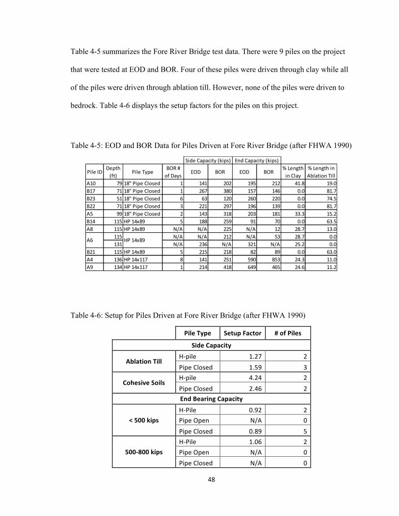
48
Table 4-5 summarizes the Fore River Bridge test data. There were 9 piles on the project
that were tested at EOD and BOR. Four of these piles were driven through clay while all
of the piles were driven through ablation till. However, none of the piles were driven to
bedrock. Table 4-6 displays the setup factors for the piles on this project.
Table 4-5: EOD and BOR Data for Piles Driven at Fore River Bridge (after FHWA 1990)
Pile IDDepth (ft)
Pile TypeBOR # of Days
EOD BOR EOD BOR% Length in Clay
% Length in Ablation Till
A10 79 18" Pipe Closed 1 141 202 195 212 41.8 19.0B17 71 18" Pipe Closed 1 267 380 157 146 0.0 81.7B23 51 18" Pipe Closed 6 63 120 260 220 0.0 74.5B22 71 18" Pipe Closed 3 221 297 196 139 0.0 81.7A5 99 18" Pipe Closed 2 143 318 203 181 33.3 15.2B14 115 HP 14x89 5 188 259 91 70 0.0 63.5A8 115 HP 14x89 N/A N/A 225 N/A 12 28.7 13.0
115 N/A N/A 212 N/A 53 28.7 0.0131 N/A 236 N/A 321 N/A 25.2 0.0
B21 115 HP 14x89 5 215 218 82 89 0.0 63.0A4 136 HP 14x117 8 141 251 590 853 24.3 11.0A9 134 HP 14x117 1 214 418 649 465 24.6 11.2
A6 HP 14x89
Side Capacity (kips) End Capacity (kips)
Table 4-6: Setup for Piles Driven at Fore River Bridge (after FHWA 1990)
Pile Type Setup Factor # of Piles
Side Capacity
Ablation Till H-‐pile 1.27 2 Pipe Closed 1.59 3
Cohesive Soils H-‐pile 4.24 2 Pipe Closed 2.46 2 End Bearing Capacity
< 500 kips H-‐Pile 0.92 2 Pipe Open N/A 0 Pipe Closed 0.89 5
500-‐800 kips H-‐Pile 1.06 2 Pipe Open N/A 0 Pipe Closed N/A 0
49
The average setup factor of 0.92 for end bearing of H-piles for capacities less than
500 k was similar to the average factor of 0.93 for the previous MaineDOT projects.
With a larger average time of 4 days from EOD to BOR compared to close to 1 day for
MaineDOT data, this indicates that there is practically no capacity change beyond 1 day.
The average setup factor of 1.06 for end bearing capacities of 500 - 800 k of H-piles
compared to 0.97 of the previous MaineDOT data indicates that the combined factor is
close to 1.0.
The average setup factor of 0.89 for 5 closed end pipe piles with capacities below
500 k was lower than the setup factor of 1.05 for 1 closed end pipe in the MaineDOT
data. This setup factor of 0.89 reflects similar behavior to the H-pile at this load level.
The closed end pipe piles experienced side capacity setup in granular soils of 1.59
similar to the 1.51 in the previous database. The side capacity setup of H-piles in
granular soils on the Fore River Bridge project was about 20% larger than the setup
factor on the other MaineDOT projects. Additionally, the side capacities of piles in
cohesive soils were also larger on the Fore River Bridge project. However, these piles
were typically tested after longer periods of time, so the larger setup factors indicate that
the piles are continuing to gain capacity after one day. It is interesting to note that the side
capacity setup of H-piles in cohesive soils was significantly larger than the closed end
pipe piles, but again the H-piles had greater setup times than the closed end pipe piles
which could account for the difference.

50
Chapter 5:
SETUP FOR END OF DRIVING CAPACITIES
5.1. Pile Setup
Piles are generally designed based on peak strength states of the soils along the
sides and end of the pile. However, MaineDOT typically uses end of driving (EOD)
capacity measurements using dynamic tests to check that the piles have obtained the
required capacity. The EOD capacities will be conservative especially in cohesive soils,
since the pile is supported by lower remolded strength at EOD. In general, the piles will
gain capacity with time as the pore pressures from driving dissipate. To assess the
reliability of the calculated ultimate capacities using peak strengths, the calculated
capacities need to be compared to a measured pile capacity at ultimate strength. The most
effective comparison is to conduct a load test after pore pressures have fully dissipated
and compare to the predicted ultimate capacity. Setup is the ratio of the capacity after
driving pore pressures have dissipated compared to EOD capacity. To determine how
much setup would ultimately be experienced by each pile after EOD, the beginning of
restrike (BOR) measurement at full dissipation can be compared to the EOD measured
capacity. The setup with time can be determined by conducting restrike tests at various
times after EOD. However, due to a lack of time dependent capacity measurements, a
method for estimating capacity with time based on the MaineDOT pile database is
presented in this chapter.
5.1.1. Setup for Cohesive Soils
When piles are driven through cohesive soil, then the piles cause remolding of the
cohesive soil close to the pile with accompanying high pore pressures. The remolded

51
strength of the Presumpscot Formation and other sensitive soils is often significantly
lower than the peak strength. However, with time after driving, the excess pore pressures
from driving will dissipate, and the remolded clay will regain its original strength. The
measured sensitivity of the cohesive soil (ratio of peak strength to remolded strength) has
been taken as the setup in the past (see Hannigan et al, 2006 p.16-20).
Bjerrum (1954) has found that the sensitivity of Norwegian clay is related to the
liquidity index (LI) of the clay.
!" =!! − !"!! − !" [5.1]
Where:
LI = Liquidity index
wn = Natural water content
PL = Plastic limit
LL = Liquid limit
Norwegian clays have a similar geologic history and similar properties to the
Presumpscot. Typically the Atterberg limits of the Presumpscot do not vary greatly, and
thus it would be expected that the clay sensitivity (and thus setup) would be primarily
related to the water content of the clay.
With the piles that had CAPWAP® data at EOD and BOR a plot was generated
that showed the ratio of BOR to EOD against water content. This plot is shown in Figure
5-1 with a line of best fit. This best fit line indicated that the magnitude of setup in
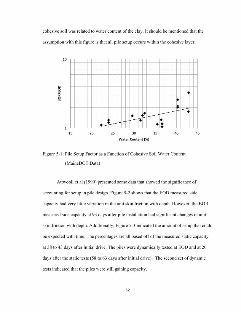
52
cohesive soil was related to water content of the clay. It should be mentioned that the
assumption with this figure is that all pile setup occurs within the cohesive layer.
Figure 5-1: Pile Setup Factor as a Function of Cohesive Soil Water Content
(MaineDOT Data)
Attwooll et al (1999) presented some data that showed the significance of
accounting for setup in pile design. Figure 5-2 shows that the EOD measured side
capacity had very little variation in the unit skin friction with depth. However, the BOR
measured side capacity at 93 days after pile installation had significant changes in unit
skin friction with depth. Additionally, Figure 5-3 indicated the amount of setup that could
be expected with time. The percentages are all based off of the measured static capacity
at 38 to 43 days after initial drive. The piles were dynamically tested at EOD and at 20
days after the static tests (58 to 63 days after initial drive). The second set of dynamic
tests indicated that the piles were still gaining capacity.
1
10
15 20 25 30 35 40 45
BOR/EO
D
Water Content (%)

53
Figure 5-2: Changes in Unit Skin Friction with Depth (Attwooll et al 1999)
Figure 5-3: Setup in Clay (Attwooll et al 1999)
Long, Kerrigan, and Wysockey (1999) also examined the amount of setup
experienced by piles in cohesive soils. Their data suggested that pile capacity will
increase rapidly with time for up to 100 days after initial driving at which point the rate
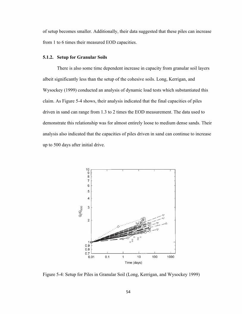
54
of setup becomes smaller. Additionally, their data suggested that these piles can increase
from 1 to 6 times their measured EOD capacities.
5.1.2. Setup for Granular Soils
There is also some time dependent increase in capacity from granular soil layers
albeit significantly less than the setup of the cohesive soils. Long, Kerrigan, and
Wysockey (1999) conducted an analysis of dynamic load tests which substantiated this
claim. As Figure 5-4 shows, their analysis indicated that the final capacities of piles
driven in sand can range from 1.3 to 2 times the EOD measurement. The data used to
demonstrate this relationship was for almost entirely loose to medium dense sands. Their
analysis also indicated that the capacities of piles driven in sand can continue to increase
up to 500 days after initial drive.
Figure 5-4: Setup for Piles in Granular Soil (Long, Kerrigan, and Wysockey 1999)

55
5.1.3. Setup for End Bearing
Based on results of MaineDOT and Fore River restrike tests on H-piles for end
bearing capacity less than 500 k, there is a loss of end bearing capacity for 1 day
restrikes, but the capacity does not continue to change beyond day one. This behavior
indicates relatively rapid pore pressure dissipation or particle adjustment after EOD.
For end bearing capacities of H-piles greater than 500 k at the sites investigated
herein, it does not appear that on average there is loss of capacity from EOD to BOR
even up to 8 days after EOD. However, these test values may not be representative of the
behavior of some shales or other weaker bedrocks that may occur in Maine.
Although the loss of bearing capacity for closed end pipe piles was similar to H-
piles for capacity levels less than 500 k, the closed end pipe pile capacity also showed
restrike loss for capacities greater than 800 k. For open pipe piles, there was not enough
data to develop separate behavior, and thus the end bearing behavior was taken to be the
same as H-pile behavior.
5.1.4. Skov and Denver Method (1988)
The most widely used method for calculating pile setup as a function of time in
soil is the method proposed by Skov and Denver (1988). The Skov and Denver method
allows for the capacity to be calculated at any time after installation. This method is
shown below:
!!!!
= 1+ ! log!!!
[5.2]
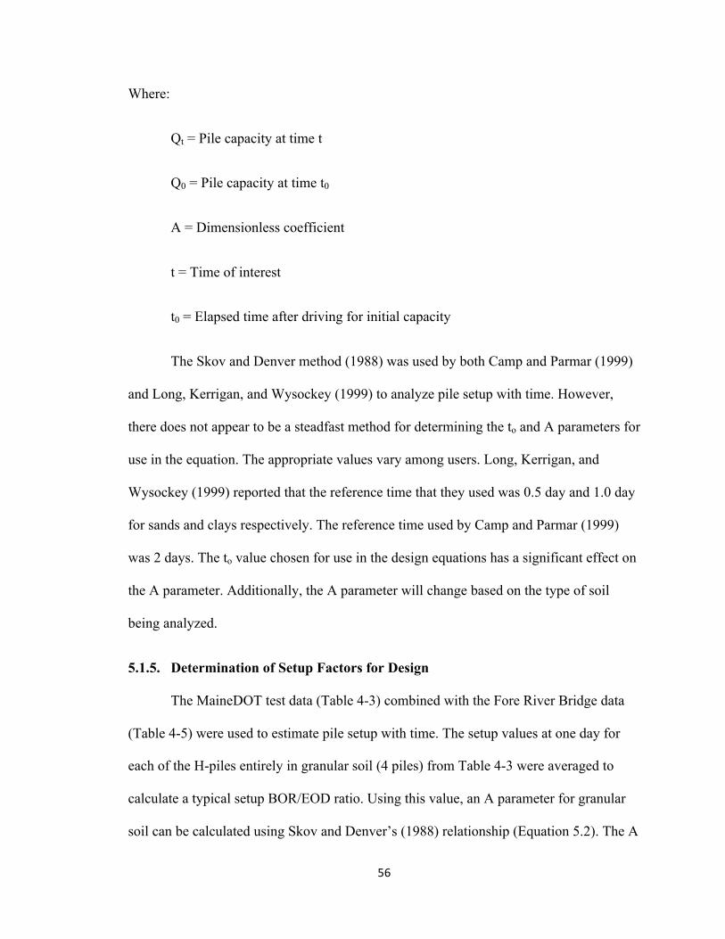
56
Where:
Qt = Pile capacity at time t
Q0 = Pile capacity at time t0
A = Dimensionless coefficient
t = Time of interest
t0 = Elapsed time after driving for initial capacity
The Skov and Denver method (1988) was used by both Camp and Parmar (1999)
and Long, Kerrigan, and Wysockey (1999) to analyze pile setup with time. However,
there does not appear to be a steadfast method for determining the to and A parameters for
use in the equation. The appropriate values vary among users. Long, Kerrigan, and
Wysockey (1999) reported that the reference time that they used was 0.5 day and 1.0 day
for sands and clays respectively. The reference time used by Camp and Parmar (1999)
was 2 days. The to value chosen for use in the design equations has a significant effect on
the A parameter. Additionally, the A parameter will change based on the type of soil
being analyzed.
5.1.5. Determination of Setup Factors for Design
The MaineDOT test data (Table 4-3) combined with the Fore River Bridge data
(Table 4-5) were used to estimate pile setup with time. The setup values at one day for
each of the H-piles entirely in granular soil (4 piles) from Table 4-3 were averaged to
calculate a typical setup BOR/EOD ratio. Using this value, an A parameter for granular
soil can be calculated using Skov and Denver’s (1988) relationship (Equation 5.2). The A

57
parameters suggested in the literature review did not come with any recommendations for
identifying which types of cohesive soils correspond to each parameter. The elapsed time
from EOD to the measurement for use in the equation was assumed to be 20 minutes
(0.014 days) (Hannigan et al 2006). The dynamic test reports generally report that the
BOR test was conducted the following calendar day from the EOD. The elapsed time was
taken to be 19 hours rather than 24 hours. It was considered that the pile was likely tested
at EOD in the afternoon (the office of the testing company is 3 to 5 hours from most
Maine locations. The technician came back in the morning to conduct the BOR test and
returned to his office (3-5 hours) following the test. This analysis produced an A
parameter of 0.042 for granular material.
A similar procedure was used to calculate the A parameters for closed end pipe
piles in granular soils and for all piles in cohesive soils. However, due to a lack of
reliable time dependent test for closed end pipe piles the test data from the Fore River
Bridge project was used. This resulted in an A parameter of 0.29. There was not
sufficient data to determine trends in cohesive setup by pile type. Instead, these A
parameters were calculated for various water contents. From the available MaineDOT
test data and the setup trend shown in Figure 5-1, it was determined that the A parameters
would be calculated for three ranges of water content: water contents < 26%, water
contents 27-39%, and water contents > 40%. The resulting A parameters were 0.061,
0.38, and 1.42 respectively.
Using the Skov and Denver (1988) relationship and the calculated A parameters,
setup factors were calculated at 0.8 days (1 day BOR), 1 day, 2 days, 3 days, 5 days, 6
days, 8 days, 14 days, 90 days, and 270 days. The 270 days as suggested by Orrje and

58
Broms (1967) for Swedish glacial clays was assumed to be the time at which the pore
pressure had fully dissipated and reached the ultimate strength state. This time was
confirmed for Maine clays through a time rate of consolidation analysis using the
following equation (Poulos and Davis 1980).
! =!!!!! [5.3]
Where:
T = time factor
a = pile radius (feet)
Ch = coefficient of horizontal consolidation (ft2/day)
The time factor can be found from the above equation for various elapsed times.
A Ch value of 0.15 ft2/day was used and was obtained from a Cv average of 0.10 ft2/day
(Andrews 1987) with a Ch/Cv = 1.5 (Poulos and Davis 1980). The relation between time
factor T and percent consolidation was used to find the consolidation for each time. It
was determined that at 289 days the pore pressure was 96% dissipated. This indicated
that the Orrje and Broms (1967) suggestion was reasonable. The resulting setup factors
from the Skov and Denver analysis are shown in Table 5-1 for various elapsed times.
The MaineDOT test data indicated that some piles will experience a reduction in
end bearing capacity from EOD to the 1 day BOR analysis as shown in Figure 4-3. These
reduction factors are shown in

59
Table 5-2. It should be noted that these factors were based only on the MaineDOT test
data which did not have any data beyond 1 day BOR for comparison. However, it is
assumed that these end setups did not change further with time.
Table 5-1: Final Time Dependent Side Capacity Setup Factors
Cohesive Factors Granular Factors
w > 40% w = 26-39% w < 26 %
HP & Open Pipe
Closed End Pipe
Time (days) Qt/Qo Qt/Qo Qt/Qo Qt/Qo Qt/Qo
0.8 3.49 1.67 1.11 1.07 1.51 1 3.63 1.70 1.11 1.08 1.54 2 4.06 1.82 1.13 1.09 1.62 3 4.31 1.89 1.14 1.10 1.68 5 4.63 1.97 1.16 1.11 1.74 6 4.74 2.00 1.16 1.11 1.76 8 4.91 2.05 1.17 1.12 1.80
14 5.26 2.14 1.18 1.13 1.87 90 6.41 2.45 1.23 1.16 2.10
270 7.09 2.63 1.26 1.18 2.24
Table 5-2: Final Bearing Capacity Setup Factors
H-Pile and Open Pipe Pile
Closed End Pipe Piles
EOD Bearing Capacity QBOR/QEOD QBOR/QEOD < 500 kips 0.92 0.92
500-800 kips 1.00 0.91 > 800 kips 1.00 0.91
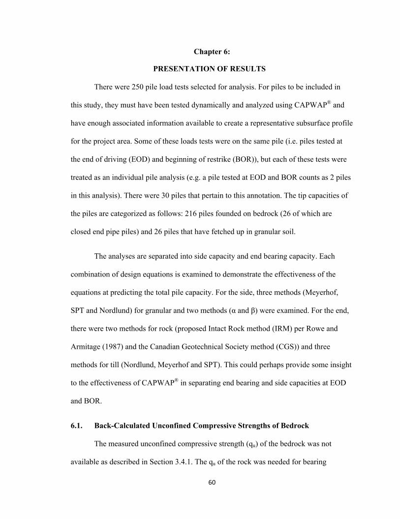
60
Chapter 6:
PRESENTATION OF RESULTS
There were 250 pile load tests selected for analysis. For piles to be included in
this study, they must have been tested dynamically and analyzed using CAPWAP® and
have enough associated information available to create a representative subsurface profile
for the project area. Some of these loads tests were on the same pile (i.e. piles tested at
the end of driving (EOD) and beginning of restrike (BOR)), but each of these tests were
treated as an individual pile analysis (e.g. a pile tested at EOD and BOR counts as 2 piles
in this analysis). There were 30 piles that pertain to this annotation. The tip capacities of
the piles are categorized as follows: 216 piles founded on bedrock (26 of which are
closed end pipe piles) and 26 piles that have fetched up in granular soil.
The analyses are separated into side capacity and end bearing capacity. Each
combination of design equations is examined to demonstrate the effectiveness of the
equations at predicting the total pile capacity. For the side, three methods (Meyerhof,
SPT and Nordlund) for granular and two methods (α and β) were examined. For the end,
there were two methods for rock (proposed Intact Rock method (IRM) per Rowe and
Armitage (1987) and the Canadian Geotechnical Society method (CGS)) and three
methods for till (Nordlund, Meyerhof and SPT). This could perhaps provide some insight
to the effectiveness of CAPWAP® in separating end bearing and side capacities at EOD
and BOR.
6.1. Back-Calculated Unconfined Compressive Strengths of Bedrock
The measured unconfined compressive strength (qu) of the bedrock was not
available as described in Section 3.4.1. The qu of the rock was needed for bearing

61
capacity calculations and thus without onsite values, these values need to be assumed
from a published range. It was desired to obtain a back-calculated qu value for specific
rock types. This value was obtained by setting Qp equal to the CAPWAP® measured end
bearing capacity and finding qu from Equation 3.15. The bedrock was categorized into
three types: igneous, metamorphic, and sedimentary rock. A weighted average of each
bedrock subtype provided a qu value for each rock type. A summary of how the rocks
were categorized and the resulting averages is shown in Table 6-1 through Table 6-3. The
average values for each rock type were then used to make an estimate of the end bearing
capacity using Equation 3.15.
Table 6-1: Back-Calculated Unconfined Compressive Strength For Igneous Bedrock
Table 6-2: Back-Calculated Unconfined Compressive Strength, Metamorphic Bedrock Metamorphic
Rock Type Number of Piles Ave (ksi) Max (ksi) Min (ksi) GNEISS 14 4.5 6.6 1.5 GRANOFELS 2 8.2 11.1 5.3 GREENSCHIST 6 4.6 5.3 4.0 HORNFELS 2 5.1 5.9 4.3 PHYLLITE 24 6.0 9.3 2.7 QUARTZITE 1 3.9 3.9 3.9 SCHIST 55 4.8 8.1 1.3 SLATE 4 7.8 9.3 5.4 All Metamorphic Rock Types 108 5.2 11.1 1.3
Igneous Rock Type Number of Piles Ave (ksi) Max (ksi) Min (ksi)
ANORTHOSITE 3 5.9 7.3 4.7 DIORITE 2 8.4 10.5 6.3 GABBRO 5 6.7 7.4 6.1 GRANITE 33 5.0 8.1 2.3 SYENITE 2 3.6 3.8 3.3 All Igneous Rock Types 45 5.4 10.5 2.3
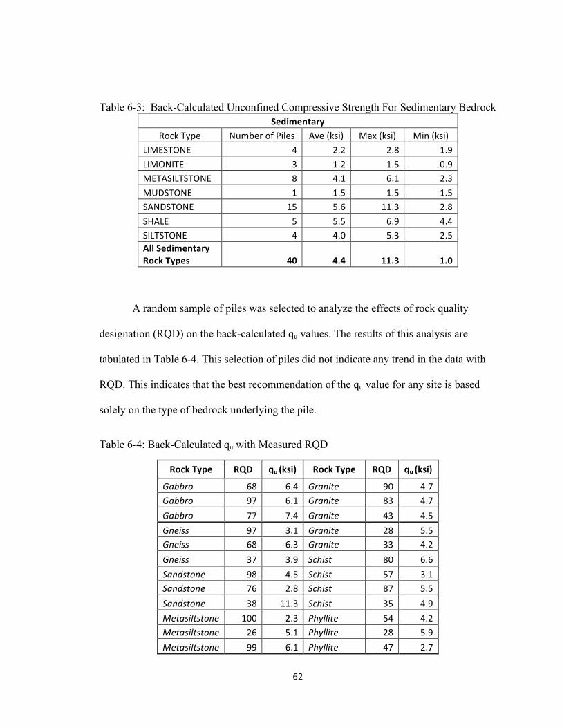
62
Table 6-3: Back-Calculated Unconfined Compressive Strength For Sedimentary Bedrock Sedimentary
Rock Type Number of Piles Ave (ksi) Max (ksi) Min (ksi) LIMESTONE 4 2.2 2.8 1.9 LIMONITE 3 1.2 1.5 0.9 METASILTSTONE 8 4.1 6.1 2.3 MUDSTONE 1 1.5 1.5 1.5 SANDSTONE 15 5.6 11.3 2.8 SHALE 5 5.5 6.9 4.4 SILTSTONE 4 4.0 5.3 2.5 All Sedimentary Rock Types 40 4.4 11.3 1.0
A random sample of piles was selected to analyze the effects of rock quality
designation (RQD) on the back-calculated qu values. The results of this analysis are
tabulated in Table 6-4. This selection of piles did not indicate any trend in the data with
RQD. This indicates that the best recommendation of the qu value for any site is based
solely on the type of bedrock underlying the pile.
Table 6-4: Back-Calculated qu with Measured RQD
Rock Type RQD qu (ksi) Rock Type RQD qu (ksi)
Gabbro 68 6.4 Granite 90 4.7 Gabbro 97 6.1 Granite 83 4.7 Gabbro 77 7.4 Granite 43 4.5 Gneiss 97 3.1 Granite 28 5.5 Gneiss 68 6.3 Granite 33 4.2 Gneiss 37 3.9 Schist 80 6.6 Sandstone 98 4.5 Schist 57 3.1 Sandstone 76 2.8 Schist 87 5.5 Sandstone 38 11.3 Schist 35 4.9 Metasiltstone 100 2.3 Phyllite 54 4.2 Metasiltstone 26 5.1 Phyllite 28 5.9 Metasiltstone 99 6.1 Phyllite 47 2.7

63
6.2. Comparison of Measured and Calculated Side Capacities
Out of the 250 piles included in the side capacity analysis, there were 2 piles that
had CAPWAP® measured side capacities of 0 kip. These piles were not included in the
presentation of results because the division by zero causes the predicted to measured ratio
to become infinite. In the side capacity calculations for open pipe piles, the soil plug was
assumed to go to the top of the pile when in reality the plugging will not completely fill
the pipe. This will likely cause an over prediction of the side capacity. The dynamically
measured side capacities from CAPWAP® analyses were factored to the 270 day ultimate
capacities using the values in Table 5-1 &
Table 5-2. These factored measured values were then compared to the calculated
ultimate side capacities from static design methods that used peak strengths. The results
of these comparisons are shown in
!"##
6.2. Comparison of Measured and Calculated Side Capacities
Out of the 250 piles included in the side capacity analysis, there were 2 piles that
had CAPWAP measured side capacities of 0 kip. These piles were not included in the
presentation of results because the division by zero causes the predicted to measured ratio
to become infinite. In the side capacity calculations for open pipe piles, the soil plug was
assumed to go to the top of the pile when in reality the plugging will not completely fill
the pipe. This will likely cause an over prediction of the side capacity The dynamically
measured side capacities from CAPWAP analyses were factored to the 270 day ultimate
capacities using the values in Table 5-1 & Table 5-2. These factored measured values
were then compared to the calculated ultimate side capacities from static design methods
that used peak strengths. The results of these comparisons are shown in Figure 6-1
through Figure 6-6. These figures each have a line which indicates equality. Each figure
has unique cases plotted separately from the typical pile behavior.
$
$%
$%%
$%%%
$%%%%
$ $% $%% $%%% $%%%%
!"#$%&'(
)*'"+,&'()-.('
)/"0
"#.$1
)23.0+4
-.(')/"0"#.$1)5&'(.#$.%6+)23.0+4
&'()*+',#-)./01'+*2.+'#3)..#4#5660/#&7/'82'(/*&9/*#-)9/#:);<#=;690&.(#>6?*#@82;A#$#-)./#"B+*++*#-)./0=<6';#-)./0#?);<#C)D<#B+9+E);)/03+.F62;<#-)./0G*E6*0)0;/*;#H/+02'/F/*;1)./+(#B/*;/'#-)/'
Figure 6-1: Nordlund and Alpha Method Side Predictions

64
Figure 6-1 through Figure 6-6. These figures each have a line which indicates
equality. Each figure has unique cases plotted separately from the typical pile behavior.
Figure 6-1: Nordlund and α Methods Side Predictions
!"##
6.2. Comparison of Measured and Calculated Side Capacities
Out of the 250 piles included in the side capacity analysis, there were 2 piles that
had CAPWAP measured side capacities of 0 kip. These piles were not included in the
presentation of results because the division by zero causes the predicted to measured ratio
to become infinite. In the side capacity calculations for open pipe piles, the soil plug was
assumed to go to the top of the pile when in reality the plugging will not completely fill
the pipe. This will likely cause an over prediction of the side capacity The dynamically
measured side capacities from CAPWAP analyses were factored to the 270 day ultimate
capacities using the values in Table 5-1 & Table 5-2. These factored measured values
were then compared to the calculated ultimate side capacities from static design methods
that used peak strengths. The results of these comparisons are shown in Figure 6-1
through Figure 6-6. These figures each have a line which indicates equality. Each figure
has unique cases plotted separately from the typical pile behavior.
$
$%
$%%
$%%%
$%%%%
$ $% $%% $%%% $%%%%
!"#$%&'(
)*'"+,&'()-.('
)/"0
"#.$1
)23.0+4
-.(')/"0"#.$1)5&'(.#$.%6+)23.0+4
&'()*+',#-)./01'+*2.+'#3)..#4#5660/#&7/'82'(/*&9/*#-)9/#:);<#=;690&.(#>6?*#@82;A#$#-)./#"B+*++*#-)./0=<6';#-)./0#?);<#C)D<#B+9+E);)/03+.F62;<#-)./0G*E6*0)0;/*;#H/+02'/F/*;1)./+(#B/*;/'#-)/'
Figure 6-1: Nordlund and Alpha Method Side Predictions
!"##
$
$%
$%%
$%%%
$%%%%
$ $% $%% $%%% $%%%%
!"#$%&'(
)*'"+,&'()-.('
)/"0
"#.$1
)23.0+4
-.(')/"0"#.$1)5&'(.#$.%6+)23.0+4
&'()*+',#-)./01'+*2.+'#3)..#4#5660/#&7/'82'(/*&9/*#-)9/#:);<#=;690&.(#>6?*#@82;A#$#-)./#BC+*++*#-)./0=<6';#-)./0#?);<#D)E<#C+9+F);)/03+.G62;<#-)./0H*F6*0)0;/*;#I/+02'/G/*;1)./+(#C/*;/'#-)/'
)
Figure 6-2: Nordlund and Beta Method Side Predictions
#
$
$%
$%%
$%%%
$%%%%
$ $% $%% $%%% $%%%%
!"#$%&'(
)*'"+,&'()-.('
)/"0
"#.$1
)23.0+4
-.(')/"0"#.$1)5&'(.#$.%6+)23.0+4
&'()*+',#-)./01'+*2.+'#3)..#4#5660/#&7/'82'(/*&9/*#-)9/#:);<#=;690&.(#>6?*#@82;A#$#-)./#BC+*++*#-)./0=<6';#-)./0#?);<#D)E<#C+9+F);)/03+.G62;<#-)./0H*F6*0)0;/*;#I/+02'/G/*;1)./+(#C/*;/'#-)/'
#
Figure 6-3: Meyerhof SPT and Alpha Method Side Predictions
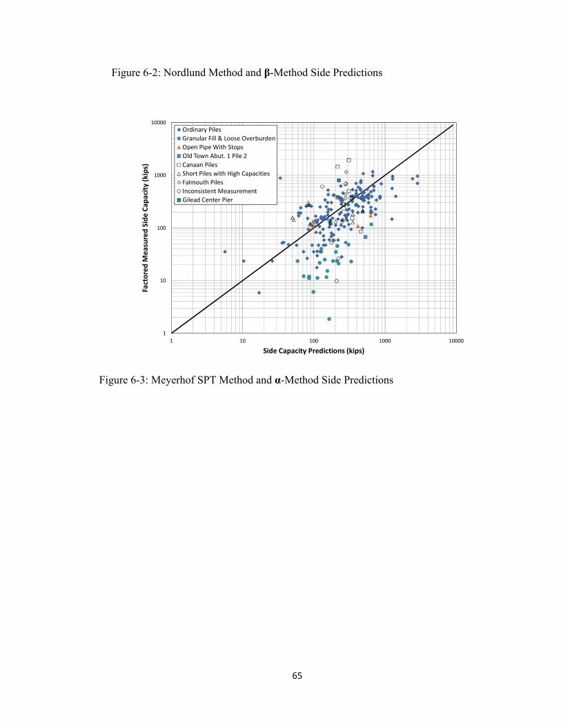
65
Figure 6-2: Nordlund Method and β-Method Side Predictions
Figure 6-3: Meyerhof SPT Method and α-Method Side Predictions
!"##
$
$%
$%%
$%%%
$%%%%
$ $% $%% $%%% $%%%%
!"#$%&'(
)*'"+,&'()-.('
)/"0
"#.$1
)23.0+4
-.(')/"0"#.$1)5&'(.#$.%6+)23.0+4
&'()*+',#-)./01'+*2.+'#3)..#4#5660/#&7/'82'(/*&9/*#-)9/#:);<#=;690&.(#>6?*#@82;A#$#-)./#BC+*++*#-)./0=<6';#-)./0#?);<#D)E<#C+9+F);)/03+.G62;<#-)./0H*F6*0)0;/*;#I/+02'/G/*;1)./+(#C/*;/'#-)/'
)
Figure 6-2: Nordlund and Beta Method Side Predictions
#
$
$%
$%%
$%%%
$%%%%
$ $% $%% $%%% $%%%%
!"#$%&'(
)*'"+,&'()-.('
)/"0
"#.$1
)23.0+4
-.(')/"0"#.$1)5&'(.#$.%6+)23.0+4
&'()*+',#-)./01'+*2.+'#3)..#4#5660/#&7/'82'(/*&9/*#-)9/#:);<#=;690&.(#>6?*#@82;A#$#-)./#BC+*++*#-)./0=<6';#-)./0#?);<#D)E<#C+9+F);)/03+.G62;<#-)./0H*F6*0)0;/*;#I/+02'/G/*;1)./+(#C/*;/'#-)/'
#
Figure 6-3: Meyerhof SPT and Alpha Method Side Predictions

66
Figure 6-4: Meyerhof SPT Method and β-Method Side Predictions
Figure 6-5: Meyerhof Method and α-Method Side Predictions
!"##
$
$%
$%%
$%%%
$%%%%
$ $% $%% $%%% $%%%%
!"#$%&'(
)*'"+,&'()-.('
)/"0
"#.$1
)23.0+4
-.(')/"0"#.$1)5&'(.#$.%6+)23.0+4
&'()*+',#-)./01'+*2.+'#3)..#4#5660/#&7/'82'(/*&9/*#-)9/#:);<#=;690&.(#>6?*#@82;A#$#-)./#BC+*++*#-)./0=<6';#-)./0#?);<#D)E<#C+9+F);)/03+.G62;<#-)./0H*F6*0)0;/*;#I/+02'/G/*;1)./+(#C/*;/'#-)/'
#
Figure 6-4: Meyerhof SPT and Beta Method Side Predictions
#
$
$%
$%%
$%%%
$%%%%
$ $% $%% $%%% $%%%%
!"#$%&'(
)*'"
+,&'()-.('
)/"0
"#.$1
)23.0+4
-.(')/"0"#.$1)5&'(.#$.%6+)23.0+4
&'()*+',#-)./01'+*2.+'#3)..#4#5660/#&7/'82'(/*&9/*#-)9/#:);<#=;690&.(#>6?*#@82;A#$#-)./#BC+*++*#-)./0=<6';#-)./0#?);<#D)E<#C+9+F);)/03+.G62;<#-)./0H*F6*0)0;/*;#I/+02'/G/*;1)./+(#C/*;/'#-)/'
Figure 6-5: Meyerhof and Alpha Method Side Predictions !"##
$
$%
$%%
$%%%
$%%%%
$ $% $%% $%%% $%%%%
!"#$%&'(
)*'"+,&'()-.('
)/"0
"#.$1
)23.0+4
-.(')/"0"#.$1)5&'(.#$.%6+)23.0+4
&'()*+',#-)./01'+*2.+'#3)..#4#5660/#&7/'82'(/*&9/*#-)9/#:);<#=;690&.(#>6?*#@82;A#$#-)./#BC+*++*#-)./0=<6';#-)./0#?);<#D)E<#C+9+F);)/03+.G62;<#-)./0H*F6*0)0;/*;#I/+02'/G/*;1)./+(#C/*;/'#-)/'
#
Figure 6-4: Meyerhof SPT and Beta Method Side Predictions
#
$
$%
$%%
$%%%
$%%%%
$ $% $%% $%%% $%%%%
!"#$%&'(
)*'"
+,&'()-.('
)/"0
"#.$1
)23.0+4
-.(')/"0"#.$1)5&'(.#$.%6+)23.0+4
&'()*+',#-)./01'+*2.+'#3)..#4#5660/#&7/'82'(/*&9/*#-)9/#:);<#=;690&.(#>6?*#@82;A#$#-)./#BC+*++*#-)./0=<6';#-)./0#?);<#D)E<#C+9+F);)/03+.G62;<#-)./0H*F6*0)0;/*;#I/+02'/G/*;1)./+(#C/*;/'#-)/'
Figure 6-5: Meyerhof and Alpha Method Side Predictions

67
Figure 6-6: Meyerhof Method and β-Method Side Predictions
6.2.1. Description of Outliers
The outliers occurring in comparisons of dynamic test capacities (with setup
applied) to calculated capacities in the figures were scrutinized to determine possible
special conditions that may not have been considered in the comparisons. Special
conditions included possible specific recurring soil profiles, abnormal construction
conditions, results from the dynamic tests that were questionable, and changed soil
profiles. The special cases found were:
1. Granular fill over soft cohesive and loose overburden over soft cohesive
2. Open pipe with stops
3. Short piles with high capacities
4. Specific project anomalies
!"##
$
$%
$%%
$%%%
$%%%%
$ $% $%% $%%% $%%%%
!"#$%&'(
)*'"+,&'()-.('
)/"0
"#.$1
)23.0+4
-.(')/"0"#.$1)5&'(.#$.%6+)23.0+4
&'()*+',#-)./01'+*2.+'#3)..#4#5660/#&7/'82'(/*&9/*#-)9/#:);<#=;690&.(#>6?*#@82;A#$#-)./#BC+*++*#-)./0=<6';#-)./0#?);<#D)E<#C+9+F);)/03+.G62;<#-)./0H*F6*0)0;/*;#I/+02'/G/*;1)./+(#C/*;/'#-)/'
#
Figure 6-6: Meyerhof and Beta Method Side Predictions
#
6.2.1. Description of Outliers
The outlying piles in the figures were analyzed to determine whether there was
justification for the poor performance of the prediction methods. The special cases found
are:
1. Granular fill over soft cohesive and loose overburden
2. Open pipe with stops
3. Short piles with high capacities
4. Specific project anomalies

68
6.2.1.1. Granular Fill Over Soft Cohesive and Loose Overburden
Some long piles had unusually low EOD measured side capacities (see Figure
4-2). Most of these low capacities appear to occur when piles are driven through granular
fill material or natural granular soils which overlie soft cohesive layers. Even when setup
was applied to the measured side capacities, the measured capacity was unusually low.
A study conducted on a test pile at the Biddeford Connector by Sandford (1989)
for the Maine Department of Transportation is relevant to the interpretation of these low
values. The Biddeford Connector is off Alfred St in Biddeford (location of a case history
in this study) and over the railroad. The test H-pile at the Biddeford Connector was
monitored with instrumentation and driven through 35 feet of sand fill over 77 feet of
clay with 5 feet of sand and gravel beneath the clay and bedrock below. The
instrumentation indicated that the 35 feet of sand fill did not contribute any downdrag
stress on the pile despite settling in excess of two feet relative to the pile during the
monitoring period. The monitoring indicated that during the driving of the pile through
the sand fill above the soft clay, a hole was created around the pile within the sand (a hole
was observed at the top of the fill). This hole stayed open by arching of the sand for the
full monitoring period of 260 days.
A study on downdrag conditions using instrumentation monitoring by Dixon
(1998) at Brunswick was done on one of the piles tested by dynamic loading for this
study (pile #6 at Rte 196, Abutment 1, Ramp B, called V2C by Dixon). The
instrumentation showed that there was no downdrag through the fill (22 ft) or in the
organic cohesive layer (10 ft) beneath the fill at the time of the dynamic test. A hole was
observed around the pile at the surface of the fill. This test together with the Biddeford

69
Connector test shows that fill can provide no frictional support. This can be part of the
explanation for the low values of side shear measured by the dynamic test on piles driven
through fill overlying soft cohesive. In the calculations, all layers were considered to be
contributing to the support of the pile. However, all pile driving does not create a hole
through the fill, so the fill layer over cohesive can not be deleted from calculations to be
comparable to the layers measured by the dynamic test.
Dixon monitored other piles besides the one that was monitored with a dynamic
test. The uncoated piles (the dynamically tested one had a bitumen coating) had side
shear stress through the fill at the time that the dynamic test was done on the other pile.
But the pile at Biddeford Connector was uncoated without showing any stress caused by
the fill. The coated pile at Brunswick continued to be monitored for 390 days. At the end
of the 390 days, there were 12 kips of downdrag indicating that the hole in the fill was
closing with time. A drop hammer started the pile at Biddeford with a continuation by a
diesel driver, while at Brunswick a vibratory hammer started the pile with a diesel driver
used to continue driving. The type of starter hammer may affect the development of the
hole in the fill around the pile.
At the Biddeford Connector, the profile was essentially fill and cohesive over
bedrock, but the profile at Brunswick was different. At Brunswick, below the fill and
organic clay there was marine sand (20 ft) and marine clay (33 ft) below the marine sand.
Following the end of driving at Brunswick, downdrag was measured in the marine sand
and in the marine clay. Thus the hole around the pile in the fill and low strength in the
soft cohesive did not extend below the first cohesive layer. The total downdrag at
Brunswick measured at the bottom of the marine clay layer after the end of driving was

70
267 kN (60 kips). This is a significant downdrag indicating the different behavior of the
lower two layers.
The piles in the loose overburden over soft cohesive or granular fill over soft
cohesive were separated from the rest of the piles, as a result of the questions raised
above about arching in the fill and low strength in the cohesive. The piles that satisfied
the filter are displayed in Figure 6-7 with the factored ultimate measured capacities on the
y-axis and the Meyerhof and α-method predicted capacities along the x-axis. The
resistance from the granular fill layer and cohesive and loose overburden and cohesive
were then removed from the calculations and compared to the factored measured
capacities. The adjusted side predictions are shown in Figure 6-8.
The results suggest that when a loose overburden or fill layer above soft clay
exists there is little contribution from the granular and also from the soft clay to the
measured side capacities. These piles were treated separately from the remaining piles.
6.2.1.2. Open Pipe with Stops
There were also some open end pipe piles that caused over predictions of the
ultimate pile side capacities. These piles were used on the Pan Am Railroad and
Veteran’s Memorial Bridges in Portland. Though the dynamic testing reports never
explicitly reported issues with the testing, the piles were unique enough to warrant erratic
predictions. These piles had stop plates welded inside the open pipe at approximately 50
feet from the tip which may have caused issues with drivability and hammer
performance. It appears that the function of these stop plates was to provide a clean upper
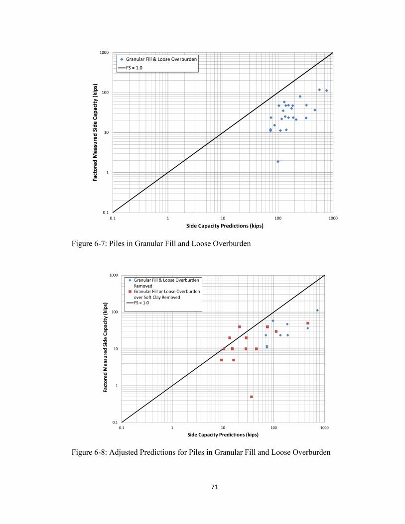
71
Figure 6-7: Piles in Granular Fill and Loose Overburden
Figure 6-8: Adjusted Predictions for Piles in Granular Fill and Loose Overburden
!"##
$%&
&
&$
&$$
&$$$
$%& & &$ &$$ &$$$
!"#$%&'(
)*'"+,&'()-.('
)/"0
"#.$1
)23.0+4
-.(')/"0"#.$1)5&'(.#$.%6+)23.0+4
'()*+,)(#-.,,#/#01123#453(6+(73*
-8#9#&%$
#
Figure 6-7: Piles in Granular Fill and Loose Overburden
#
$%&
&
&$
&$$
&$$$
$%& & &$ &$$ &$$$
!"#$%&'(
)*'"+,&'()-.('
)/"0
"#.$1
)23.0+4
-.(')/"0"#.$1)5&'(.#$.%6+)23.0+4
'()*+,)(#-.,,#/#01123#453(6+(73*#:3;1537'()*+,)(#-.,,#1(#01123#453(6+(73*#153(#81<=#>,)?#:3;1537-8#9#&%$
#
Figure 6-8: Adjusted Predictions for Piles in Granular Fill and Loose Overburden

72
section to receive concrete for additional lateral stability. The additional resistance
generated with this plate prevented the specified hammer from effectively driving the pile
and required a switching of hammers during the test. As a result of the somewhat erratic
capacity of this type of pile, they were removed from the correlations.
6.2.1.3. Short Piles
Another set of piles which resulted in conservative predictions by some methods
were short piles with unexpectedly high side capacities at Georgetown, Fryeburg and
Auburn. The Nordlund and Meyerhof methods significantly under predicted the
measured side capacities. These piles were generally less than 20 or 30 feet long with
measured capacities greater than 100 kips of skin friction measured by the CAPWAP®
analysis. Additionally, the boring logs for these piles indicated that they were generally
driven through soft/loose silts and/or loose to medium dense sands that typically will not
result in these large capacities. Perhaps there are limitations in predicting side capacity
with CAPWAP® when piles are short with high end bearing on competent bedrock.
6.2.1.4. Specific Case Anomalies
A case of over prediction is the Irving Bridge in Old Town. The pile was located
in the Abutment 1 substructure, and the analysis significantly over predicted the pile
capacity. According to the boring the pile was driven through a dense till layer, but it
would appear that the measured capacity does not reflect that resistance. The tested pile
in the Abutment 2 substructure was approximately 18 feet shorter than the Abutment 1
pile and according to the boring was not driven through till. However, it had a capacity
twice as large as the Abutment 1 pile.

73
The Boothbay Knickerbocker Bridge alignment was located downstream of the
provided subsurface investigation alignment. There were some conflicting elevations
reported in the geotechnical report as compared to the dynamic testing reports at the
bridge alignment. The conflicting elevations greatly affected which soil layers would
contribute to the side resistance because there were highly sloping bedrock and dense
sand layers.
On the project in Grand Lake Stream there were two piles tested at each of the
abutment structures which were driven through similar subsurface profiles. One pile was
22.5 feet long and measured 20 kips of skin friction at EOD, the other pile was 30.3 feet
long and measured 520 kips at EOD. A difference of 500 kips in skin friction
measurement for 8 feet difference in pile length is counterintuitive. The same situation
was observed at the MCRR Bridge in Yarmouth. There were also some piles on the
Bartlett Bridge and Center Street Bridge in New Portland and Auburn respectively which
exhibited little to no side capacity.
Some of the figures also show some data which indicate some very conservative
predictions. One of these projects is the Sibley Pond Bridge in Canaan. This project had a
few piles that had significant drops in side capacity from EOD to 1 day BOR. The
dynamic test report indicated that after the pile was allowed setup, the hammer may not
have been able to activate the total side resistance which likely led to the under predicted
capacities upon restrike.
The Falmouth Railroad Crossing Bridge over Presumpscot River Bridge produced
erratic results. The reported results claimed that the side capacity of the piles had

74
increased by 200-300 kips and the end bearing capacities had decreased by 200-300 kips
overnight. This drastic change indicates unnatural soil behavior and an error in the
analysis or presentation of the data. One possible cause was that when some of the first
piles driven on the site were not achieving the required capacity, it was decided to change
to a larger hammer to redrive the piles.
On the Wild River Bridge project in Gilead, one of the piles located in the Center
Pier substructure had an odd distribution of skin friction along the side of the pile. The
dynamic test for the pile reported that 550 kips developed along the bottom 7 feet of the
pile in a very dense till stratum. The density of this layer was considered in design;
however, the predicted skin friction due to the dense till was far below the measured
amount. The boring logs indicated the presence of cobbles which required drilling during
the subsurface exploration. Perhaps the pile was wedged between some cobbles along the
bottom of the pile. The pile was reported to be caught up on bedrock at an elevation 10
feet above the reported bedrock elevation in the corresponding boring log. The reported
end bearing capacity of 450 kips is also lower than other piles which were claimed to be
resting on bedrock.

75
6.2.2. Analysis of Predictions with Outliers Removed
6.2.2.1. Presentation of Results
The previously discussed outliers in side shear capacity were removed from the
measured test data for use in the method comparison. The predicted side shear capacities
by equations were compared to the dynamic test results. A best fit trend line was put
through each data set, and a standard error from the best fit was determined to describe
the quality of the fit. Additionally to compare the effectiveness of each prediction, the
standard deviation of the data from the line representing equality between predicted and
measured was determined for each data set. The plots used in comparing the effectiveness
of each method are shown in Figure 6-9 through Figure 6-14.
Figure 6-9: Nordlund Method and α-Method Combined Side Capacity Predictions with
Outliers Removed
!"##
6.2.2. Analysis of Predictions with Outliers Removed
6.2.2.1. Presentation of Results #
The previously discussed outliers in side shear were removed from the measured
test data for use in the method comparison. The predicted side shear by equations was
compared to the dynamic test results. A best fit trend line was put through each data set,
and a standard error from the best fit was determined to describe the quality of the fit.
Additionally to compare the effectiveness of each prediction, the standard deviation of
the data from the line representing equality between predicted and measured was
determined for each data set. The plots used in comparing the effectiveness of each
method are shown in Figure 6-9 through Figure 6-14.
$
%$$
&$$$
&%$$
"$$$
"%$$
$ %$$ &$$$ &%$$ "$$$ "%$$
!"#$%&'(
)*'"+,&'()-.('
)/"0
"#.$1
)23.0+4
-.(')/"0"#.$1)5&'(.#$.%6+)23.0+4
'(#&)$
*+,-./#0-12#'+2
#
Figure 6-9: Nordlund and Alpha Method Combined Side Capacity Predictions with
Outliers Removed

76
Figure 6-10: Nordlund Method and β-Method Combined Side Capacity Predictions with
Outliers Removed
Figure 6-11: Meyerhof SPT Method and α-Method Combined Side Capacity Predictions
with Outliers Removed
!"##
$
%$$
&$$$
&%$$
'$$$
'%$$
$ %$$ &$$$ &%$$ '$$$ '%$$
!"#$%&'(
)*'"+,&'()-.('
)/"0
"#.$1
)23.0+4
-.(')/"0"#.$1)5&'(.#$.%6+)23.0+4
()#&*$
+,-./0#1.23#(,3
#
Figure 6-10: Nordlund and Beta Method Combined Side Capacity Predictions with
Outliers Removed
$
%$$
&$$$
&%$$
'$$$
'%$$
$ %$$ &$$$ &%$$ '$$$ '%$$
!"#$%&'(
)*'"+,&'()-.('
)/"0
"#.$1
)23.0+4
-.(')/"0"#.$1)5&'(.#$.%6+)23.0+4
()#&*$
+,-./0#1.23#(,3
#
Figure 6-11: Meyerhof SPT and Alpha Method Combined Side Capacity Predictions with
Outliers Removed))
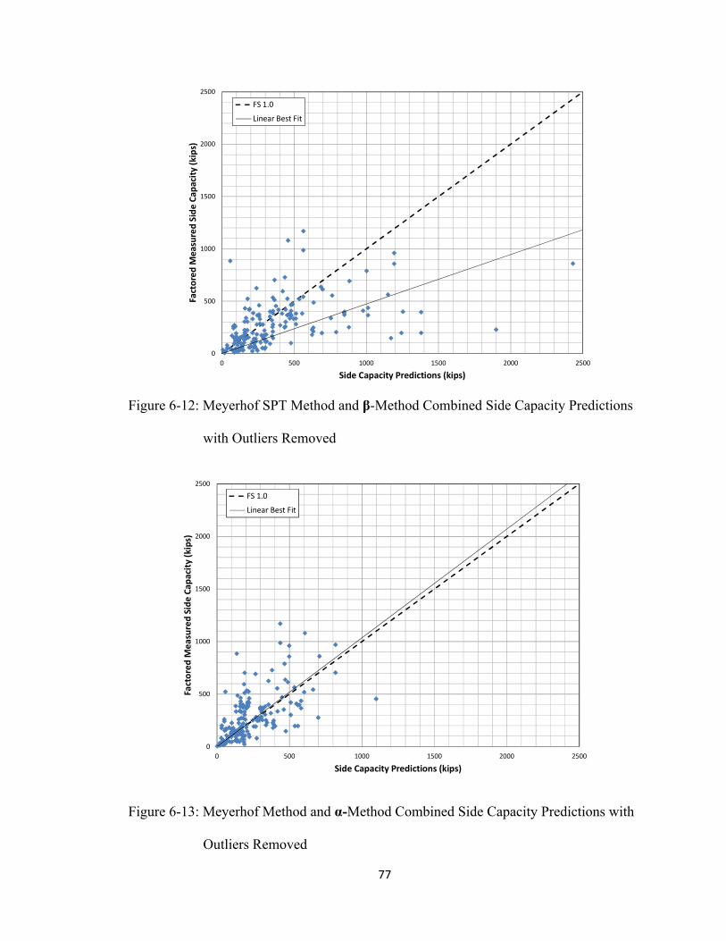
77
Figure 6-12: Meyerhof SPT Method and β-Method Combined Side Capacity Predictions
with Outliers Removed
Figure 6-13: Meyerhof Method and α-Method Combined Side Capacity Predictions with
Outliers Removed
!
"!!
#!!!
#"!!
$!!!
$"!!
! "!! #!!! #"!! $!!! $"!!
!"#$%&'(
)*'"+,&'()-.('
)/"0
"#.$1
)23.0+4
-.(')/"0"#.$1)5&'(.#$.%6+)23.0+4
%&'#(!
)*+,-.'/,01'%*1
'
!"##
$
%$$
&$$$
&%$$
'$$$
'%$$
$ %$$ &$$$ &%$$ '$$$ '%$$
!"#$%&'(
)*'"+,&'()-.('
)/"0
"#.$1
)23.0+4
5&'(.#$'()-.(')/"0"#.$1)23.0+4
()#&*$
+,-./0#1.23#(,3
)
Figure 6-12: Meyerhof SPT and Beta Method Combined Side Capacity Predictions with
Outliers Removed)
$
%$$
&$$$
&%$$
'$$$
'%$$
$ %$$ &$$$ &%$$ '$$$ '%$$
!"#$%&'(
)*'"+,&'()-.('
)/"0
"#.$1
)23.0+4
-.(')/"0"#.$1)5&'(.#$.%6+)23.0+4
()#&*$
+,-./0#1.23#(,3
#
Figure 6-13: Meyerhof and Alpha Method Combined Side Capacity Predictions with
Outliers Removed))

78
Figure 6-14: Meyerhof Method and β-Method Combined Side Capacity Predictions with
Outliers Removed
The quality of each best fit line is presented in Table 6-5. It is immediately
evident that the Meyerhof method coupled with the α-method for cohesive soils had the
most reliable best fit line. The slope of the best fit line for the Meyerhof and α-method
was 1.04 which is close to the line of equality having a slope of 1.0. The slopes of the
best fit lines for the other methods showed that on average the other methods
overestimated the side capacity of the pile by 1.5-2.8 times. The slope of the best fit lines
for methods containing the α-method for cohesive were always closer to the equality line
than those methods containing the β-method for cohesive. Likewise the slope for the best
fit lines for methods containing the Meyerhof method for granular were closer to the
equality line than either the Standard Penetration Test (SPT) or the Nordlund method,
with the Nordlund method being further away than the SPT method.
!"##
$
"$$
%$$$
%"$$
&$$$
&"$$
$ "$$ %$$$ %"$$ &$$$ &"$$
!"#$%&'(
)*'"+,&'()-.('
)/"0
"#.$1
)23.0+4
-.(')/"0"#.$1)5&'(.#$.%6+)23.0+4
'(#%)$
*+,-./#0-12#'+2
)
Figure 6-14: Meyerhof and Beta Method Combined Side Capacity Predictions with
Outliers Removed)
# The quality of each best fit line is presented in Table 6-5. It is immediately
evident that the Meyerhof Method coupled with the Alpha Method for cohesive soils had
the most reliable best fit line. The slope of the best fit line for the Meyerhof and Alpha
Method was 1.04 which is close to the line of equality having a slope of 1.0. The slopes
of the best fit lines for the other methods showed that on average the other methods
overestimated the side capacity of the pile by 1.5-2.8 times. The slope of the best fit lines
for methods containing the Alpha Method for cohesive were always closer to the equality
line than those methods containing the Beta Method for cohesive. Likewise the slope for
the best fit lines for methods containing the Meyerhof Method for granular were closer to
the equality line than either the SPT or the Nordlund Method, with the Nordlund Method
being further away than the SPT Method.

79
Table 6-5: Description of Best Fit Line for Side Capacity Prediction Method
Nordlund + α
Nordlund + β
Meyerhof SPT + α
Meyerhof SPT + β
Meyerhof + α
Meyerhof + β
Slope 0.40 0.36 0.53 0.47 1.04 0.67 Std. Error of Regression
(kips) 203.17 214.23 220.43 231.51 188.18 249.10
R2 0.68 0.65 0.64 0.60 0.73 0.52
Even the scatter around the best fit line for the Meyerhof and α-method was the
least of all best fit lines. The line had the smallest standard error and coefficient of
determination R2 value that was closest to 1.0. However, the data around the best fit line
still showed significant scatter with a relative standard error of 33% (standard
error/mean). It was also interesting to note that the scatter around the best fit lines for the
Meyerhof SPT based methods were worse than the best fit lines for the Nordlund method.
The effectiveness of each prediction method was evaluated by comparing the
standard error of each method’s data to the line of equality rather than the best fit line.
The standard error relative to the line of equality for each prediction method is displayed
in Table 6-6. The Meyerhof method + α-method was determined to have predictions
closest to the line of equality. This method had a standard error from the line of equality
that was approximately 100 kips closer than any of the other prediction methods. The
data also indicated that the comparisons using the α-method on average had prediction
errors approximately 70 kips less than the β-method predictions using corresponding
prediction methods for granular material. Furthermore, it was readily evident that the
Meyerhof based predictions had the smallest error and the Nordlund based predictions
had the largest error. The Nordlund based errors were on the order of 2.25 larger than the

80
Meyerhof based errors. The strength of the Meyerhof method is that it has a limiting
stress value with depth which is not applied to the Nordlund method. The Meyerhof,
Nordlund and α-method predictions will likely improve as the quality of the soil
properties increase while the SPT method and β-method will not. These predictions used
soil properties for granular soils correlated from SPT N-values, but if the properties were
measured directly the predictions would likely improve.
The relative standard error is an indicator of the precision of the estimates made
by each combination of methods. The analysis of each method’s predictions versus the
equality line indicated that none of the methods showed much precision, but when
compared to each other it was evident that the Meyerhof method and α-method
combination was most precise. It was the only method with less than 100% relative
standard error. This statistic also indicated that the β-method for cohesive soil and
Nordlund method for granular soil were least precise. The relative standard error could be
important for determining an appropriate factor of safety to be applied to each method’s
prediction.
Table 6-6: Standard Error in Side Capacity Estimates Relative to Line of Equality
Nordlund + α
Nordlund + β
Meyerhof SPT + α
Meyerhof SPT + β
Meyerhof + α
Meyerhof + β
Std Error from
Equality Line
488 kips 549 kips 338 kips 393 kips 189 kips 280 kips
Rel. Std Error from
Equality Line, %
175 197 122 142 68 101
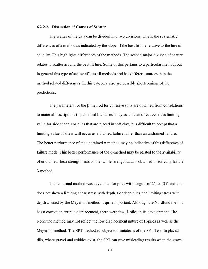
81
6.2.2.2. Discussion of Causes of Scatter
The scatter of the data can be divided into two divisions. One is the systematic
differences of a method as indicated by the slope of the best fit line relative to the line of
equality. This highlights differences of the methods. The second major division of scatter
relates to scatter around the best fit line. Some of this pertains to a particular method, but
in general this type of scatter affects all methods and has different sources than the
method related differences. In this category also are possible shortcomings of the
predictions.
The parameters for the β-method for cohesive soils are obtained from correlations
to material descriptions in published literature. They assume an effective stress limiting
value for side shear. For piles that are placed in soft clay, it is difficult to accept that a
limiting value of shear will occur as a drained failure rather than an undrained failure.
The better performance of the undrained α-method may be indicative of this difference of
failure mode. This better performance of the α-method may be related to the availability
of undrained shear strength tests onsite, while strength data is obtained historically for the
β-method.
The Nordlund method was developed for piles with lengths of 25 to 40 ft and thus
does not show a limiting shear stress with depth. For deep piles, the limiting stress with
depth as used by the Meyerhof method is quite important. Although the Nordlund method
has a correction for pile displacement, there were few H-piles in its development. The
Nordlund method may not reflect the low displacement nature of H-piles as well as the
Meyerhof method. The SPT method is subject to limitations of the SPT Test. In glacial
tills, where gravel and cobbles exist, the SPT can give misleading results when the gravel

82
and cobble particles are bigger than the split spoon opening. Different kinds of split
spoons and hammers used in the SPT can affect the ability of the measurements to
produce consistent and repeatable correlations.
For scatter around the best fit lines, there are a number of possible limitations of
the properties or methods to obtain property values that can cause scatter. The horizontal
earth pressure (Kh) used in the Meyerhof method and also in the Nordlund method were
taken from typical ranges and were not measured. This is especially relevant for basal till
where the Kh value may be quite high and where much side support is found. The peak
drained friction angle for each granular layer was obtained from correlations to SPT. The
above noted limitations to SPT will affect obtaining a representative friction angle from
SPT. The values of pile-soil interface friction angle were taken from historical values
which are given in ranges. It is not known where in the range that Maine soils may be. A
constant of friction angle for glacial till (obtained from the literature) was used.
Variations in this friction angle will affect the side capacity.
The setup factors applied to the CAPWAP® measured values were developed
from limited EOD/BOR data where most of the BOR values were taken the day
following the EOD. Although the extrapolations to an anticipated 95% consolidation
setup at 270 days appears reasonable, differences in consolidation rate can change the
number of days to 95% setup. Although the change with time of setup by Skov and
Denver is used by others and appears reasonable in the literature, it is still an
extrapolation based on limited data to obtain the A factor.
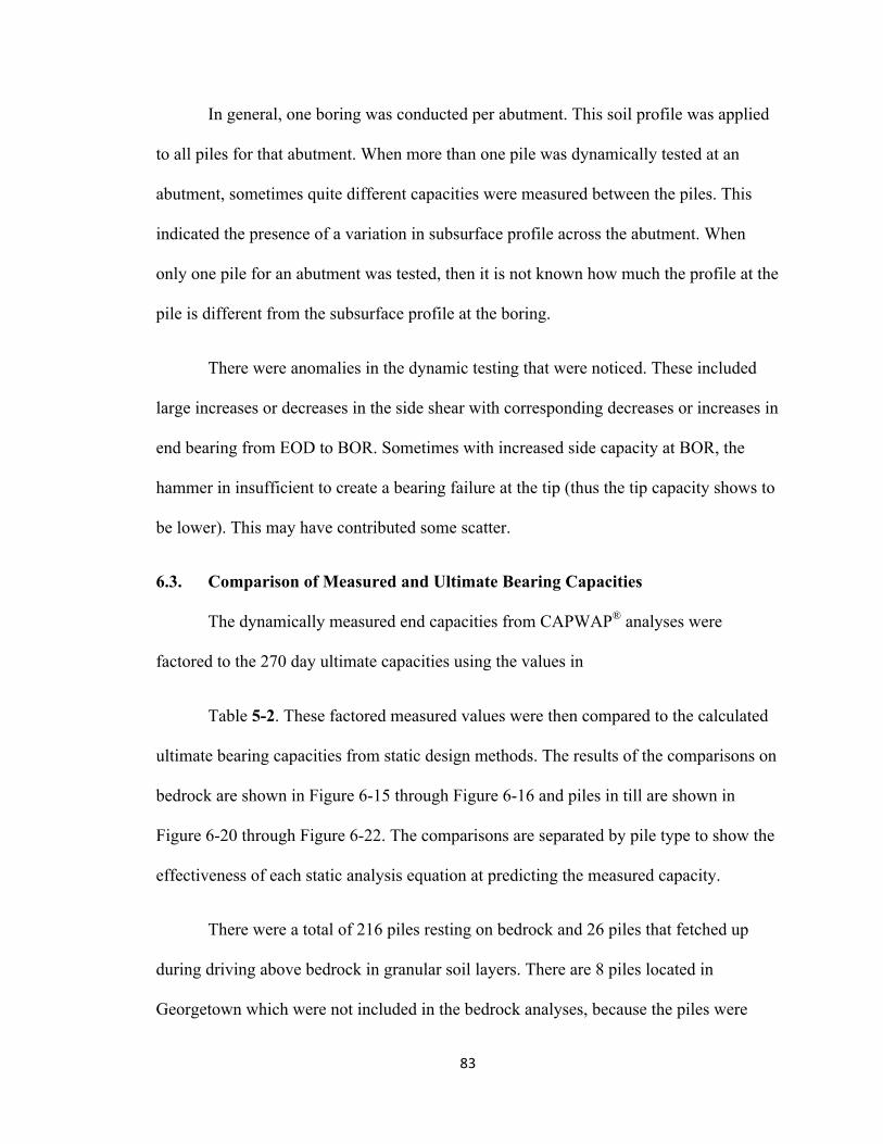
83
In general, one boring was conducted per abutment. This soil profile was applied
to all piles for that abutment. When more than one pile was dynamically tested at an
abutment, sometimes quite different capacities were measured between the piles. This
indicated the presence of a variation in subsurface profile across the abutment. When
only one pile for an abutment was tested, then it is not known how much the profile at the
pile is different from the subsurface profile at the boring.
There were anomalies in the dynamic testing that were noticed. These included
large increases or decreases in the side shear with corresponding decreases or increases in
end bearing from EOD to BOR. Sometimes with increased side capacity at BOR, the
hammer in insufficient to create a bearing failure at the tip (thus the tip capacity shows to
be lower). This may have contributed some scatter.
6.3. Comparison of Measured and Ultimate Bearing Capacities
The dynamically measured end capacities from CAPWAP® analyses were
factored to the 270 day ultimate capacities using the values in
Table 5-2. These factored measured values were then compared to the calculated
ultimate bearing capacities from static design methods. The results of the comparisons on
bedrock are shown in Figure 6-15 through Figure 6-16 and piles in till are shown in
Figure 6-20 through Figure 6-22. The comparisons are separated by pile type to show the
effectiveness of each static analysis equation at predicting the measured capacity.
There were a total of 216 piles resting on bedrock and 26 piles that fetched up
during driving above bedrock in granular soil layers. There are 8 piles located in
Georgetown which were not included in the bedrock analyses, because the piles were

84
founded on highly sloping bedrock. This indicated that they would not achieve the full
bearing area on bedrock. There were only 179 piles included in the end bearing analysis
using the CGS method. The pile deficit is due to a lack of information about the bedrock
joints in the project documents provided by MaineDOT. Without this information
predictions about the capacity of the pile could not be determined.
6.3.1. Comparison for Piles Bearing on Bedrock
The factored measured end bearing capacities for piles resting on bedrock were
compared to predicted pile capacities using the CGS and proposed IRM. The results of
the comparisons are shown in Figure 6-15 and Figure 6-16. The piles were plotted
separately for closed end pipe piles, H-piles and open end pipe piles to investigate the
effects of bearing area on the predicted capacities.
Upon inspection of the capacity comparison plots, it was evident that the
proposed IRM, per Rowe and Armitage (1987), produced the better predictions. In the
proposed IRM, an average rock effective unconfined strength based upon rock type
(sedimentary, metamorphic, or igneous) is used to find the bearing capacity of the rock.
This effective average unconfined strength was derived from the existing database of
dynamic end bearing measurements. Therefore the average calculated bearing for each
rock type should be close to the line of equality, but the variability around the mean is
important for this simplified method. However, when the variability of the proposed IRM
is compared to the variability of the CGS method, there is greater variability in the CGS
method despite the CGS method considering more variables than the proposed IRM.
There are too many unknowns with the CGS method to make reliable predictions.
Estimations about parameters for the rock mass need to be made from small rock cores or

85
in the case of this report from bedrock descriptions in the boring logs. Some of the
parameters, such as discontinuity opening, are not found with traditional subsurface
investigations. Additionally, the unconfined compressive strengths of the bedrock are
taken from published ranges.
There are some conflicting trends shown in the results of each method. The
proposed IRM indicated that open end pipe piles achieved larger bearing capacities on
bedrock than closed end pipe piles and H-piles, but the CGS method predicted that the
closed end pipe piles would have much larger pile capacities. The CGS trend is the most
sensible because closed end pipe piles have the largest cross sectional area. However, the
open end pipe piles generally had the highest measured bearing capacities as shown in the
proposed IRM predictions. It is intuitive that the open end pipe piles have larger
measured capacities than the H-piles because the cross sectional area of steel is larger for
the open end pipe piles. The lower closed end pipe pile capacities may be
counterintuitive, but are likely due to the fact that a reduction factor of 9.3 was applied to
the proposed IRM predictions as explained in Section 3.4.1. The reduction factor was
used to ensure that the closed end pipe piles could use the same back-calculated qu values
as for low displacement piles. It was assumed that the pile tip fully penetrated the
bedrock, so the full cross section of the pipe was used as the bearing area of the pile.
Some of the scatter of both methods may be caused by some piles fetching up in
till while they were calculated to bearing on rock. The dividing line between a pile that
ends in till and one that ends on rock is not well defined. Some of the lower measured
rock values may have actually been terminated in till.
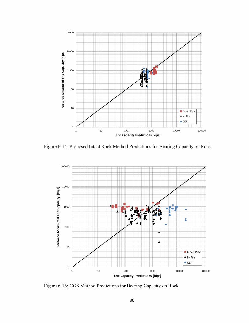
86
Figure 6-15: Proposed Intact Rock Method Predictions for Bearing Capacity on Rock
Figure 6-16: CGS Method Predictions for Bearing Capacity on Rock
!"##
$
$%
$%%
$%%%
$%%%%
$%%%%%
$ $% $%% $%%% $%%%% $%%%%%
!"#$%&'(
)*'"+,&'()-.
()/"
0"#1$2)3410+5
-.()/"0"#1$2)6&'(1#$1%.+)3410+5
&'()#*+'(
,-*+.(
/0*
#
Figure 6-15: Intact Rock Method Predictions for Bearing Capacity on Rock
$
$%
$%%
$%%%
$%%%%
$%%%%%
!"#$%&'(
)*'"+,&'()-.
()/"
0"#1$2)3410+5
&'()#*+'(
,-*+.(
/0*#
Figure 6-16: CGS Method Predictions for Bearing Capacity on Rock
!"##
$
$%
$%%
$%%%
$%%%%
$%%%%%
$ $% $%% $%%% $%%%% $%%%%%
!"#$%&'(
)*'"+,&'()-.()/"0"#1$2)3410+5
-.()/"0"#1$2)6&'(1#$1%.+) 3410+5
&'()#*+'(
,-*+.(
/0*
#
Figure 6-15: Intact Rock Method Predictions for Bearing Capacity on Rock
$
$%
$%%
$%%%
$%%%%
$%%%%%
$ $% $%% $%%% $%%%% $%%%%%
!"#$%&'(
)*'"+,&'()-.()/"0"#1$2)3410+5
-.()/"0"#1$2)6&'(1#$1%.+) 3410+5
&'()#*+'(
,-*+.(
/0*
#
Figure 6-16: CGS Method Predictions for Bearing Capacity on Rock

87
6.3.2. Comparison for Piles Bearing in Till
A difference in the pile bearing capacities existed depending on the type of
materials in the bearing strata. This led to an analysis on the effect of the pile bearing area
and soil composition on predicting the measured capacities. The results of these analyses
are shown in Figure 6-17 through Figure 6-19. The data suggested that generally the
coarse grained till material (which sometimes included cobbles) had better predictions of
the measured capacity when a box perimeter (H-piles) or closed pipe area (open end pipe
piles) was used as the bearing area. The cross sectional area of the steel provided the best
prediction for fine grained tills such as dense clayey, silty, or fine sandy material. These
respective areas were used for the comparisons. If strength tests confirm a difference of
friction angle for these two tills, then this correction must be reexamined. There were not
any changes made to the bearing area for the closed end pipe piles because there is no
chance of plugging like there is with the low displacement piles.
Figure 6-17: Effect of Grain Size on Meyerhof Bearing Predictions in Till
!"##
6.3.2. Comparison for Piles Bearing in Till
A difference in the pile bearing capacities existed depending on the type of
materials in the bearing strata. This led to an analysis on the effect of the pile bearing area
and soil composition on predicting the measured capacities. The results of these analyses
are shown in Figure 6-17 through Figure 6-19. The data suggested that generally the
coarse grained till material (which sometimes included cobbles) had better predictions of
the measured capacity when a box perimeter (H-piles) or closed pipe area (open end pipe
piles) was used as the bearing area. The cross sectional area of the steel provided the best
prediction for fine grained tills such as dense clayey, silty, or fine sandy material. These
respective areas were used for the comparisons. If strength tests confirm a difference of
friction angle for these two tills, then this correction must be reexamined. There were not
any changes made to the bearing area for the closed end pipe piles because there is no
chance of plugging like there is with the low displacement piles.
$
%$$
"$$
&$$
!$$
'$$$
'%$$
$ %$$ "$$ &$$ !$$ '$$$ '%$$
!"#$%&'(
)*'"+,&'()-.()/"
0"#1$2)3410+5
-.()/"0"#1$2)6&'(1#$1%.+)3410+5
()*+,-#.+*/0-1#2/33#4 53677-1#8+-*()*+,-#.+*/0-1#2/33#4 9:--3#8+-*;/0-#.+*/0-1#2/33#4 53677-1#8+-*;/0-#.+*/0-1#2/33#4 9:--3#8+-*
#
Figure 6-17: Effect of Grain Size on Meyerhof Bearing Predictions in Till

88
Figure 6-18: Effect of Grain Size on Nordlund Bearing Predictions in Till
Figure 6-19: Effect of Grain Size on Meyerhof SPT Bearing Predictions in Till
!"##
$
%$$
&$$
'$$
!$$
($$$
(%$$
$ %$$ &$$ '$$ !$$ ($$$ (%$$
!"#$%&'(
)*'"+,&'()-.
()/"
0"#1$2)34
10+5
-.()/"0"#1$2)6&'(1#$1%.+)3410+5
)*+,-.#/,+01.2#3044#5 64788.2#9,.+)*+,-.#/,+01.2#3044#5 :;..4#9,.+<01.#/,+01.2#3044#5 64788.2#9,.+<01.#/,+01.2#3044#5 :;..4#9,.+
#
Figure 6-18: Effect of Grain Size on Nordlund Bearing Predictions in Till
#
$
%$$
&$$
'$$
!$$
($$$
(%$$
$ %$$ &$$ '$$ !$$ ($$$ (%$$
!"#$%&'()*
'"+,&'()-.()/"0"#1$2)3410
+5
-.()/"0"#1$2) 6&'(1#$1%.+) 3410+5
)*+,-. #/,+01.2#3044#5 64788.2#9,.+)*+,-. #/,+01.2#3044#5 :;.. 4#9,.+< 01.#/,+01.2#3044 #5 64788.2#9,.+< 01.#/,+01.2#3044 #5 :;..4#9,.+
#
Figure 6-19: Effect of Grain Size on Meyerhof SPT Bearing Predictions in Till
!"##
$
%$$
&$$
'$$
!$$
($$$
(%$$
$ %$$ &$$ '$$ !$$ ($$$ (%$$
!"#$%&'(
)*'"+,&'()-.()/"0"#1$2)3410+5
-.()/"0"#1$2)6&'(1#$1%.+) 3410+5
)*+,-.#/,+01.2#3044#5 64788.2#9,.+)*+,-.#/,+01.2#3044#5 :;..4#9,.+<01.#/,+01.2#3044#5 64788.2#9,.+<01.#/,+01.2#3044#5 :;..4#9,.+
#
Figure 6-18: Effect of Grain Size on Nordlund Bearing Predictions in Till
#
$
%$$
&$$
'$$
!$$
($$$
(%$$
$ %$$ &$$ '$$ !$$ ($$$ (%$$
!"#$%&'(
)*'"+,&'()-.()/"0"#1$2)3410+5
-.()/"0"#1$2)6&'(1#$1%.+) 3410+5
)*+,-.#/,+01.2#3044#5 64788.2#9,.+)*+,-.#/,+01.2#3044#5 :;..4#9,.+<01.#/,+01.2#3044#5 64788.2#9,.+<01.#/,+01.2#3044#5 :;..4#9,.+
#
Figure 6-19: Effect of Grain Size on Meyerhof SPT Bearing Predictions in Till

89
The ultimate pile tip capacities in till were predicted using the Meyerhof,
Nordlund, and Meyerhof SPT analyses and compared to the dynamically measured
capacity at 270 days using the setup factors presented in Section 5.1.5. The results of the
till comparisons are shown in Figure 6-20 through Figure 6-22. The Meyerhof and
Nordlund methods provided very similar comparisons, while the SPT based method
showed some more scatter in its predictions. The similarities of the Meyerhof and
Nordlund methods are not coincidental. The assumed friction angle of 38° for dense to
very dense tills and the limiting values allow for little deviation in the predictions. The
limiting criterion used in recent versions of Nordlund’s method is the same as for the
Meyerhof method. The SPT based analysis shows more scatter in its predictions due to
the variability of the SPT readings from pile to pile. The use of a constant friction angles
within the till layers eliminates the scatter from the Nordlund and Meyerhof predictions,
however, this does not necessarily mean that these values are more reliable.
The bearing capacity predictions for the open end pipe piles are a little low. This
may be related to using the steel area as the bearing area. There is likely some resistance
due to the soil plug which has formed inside the pile. Not considering the plug for
bearing potentially under predicts the end bearing capacity. The plug in the pile should
pick up some of the bearing load.
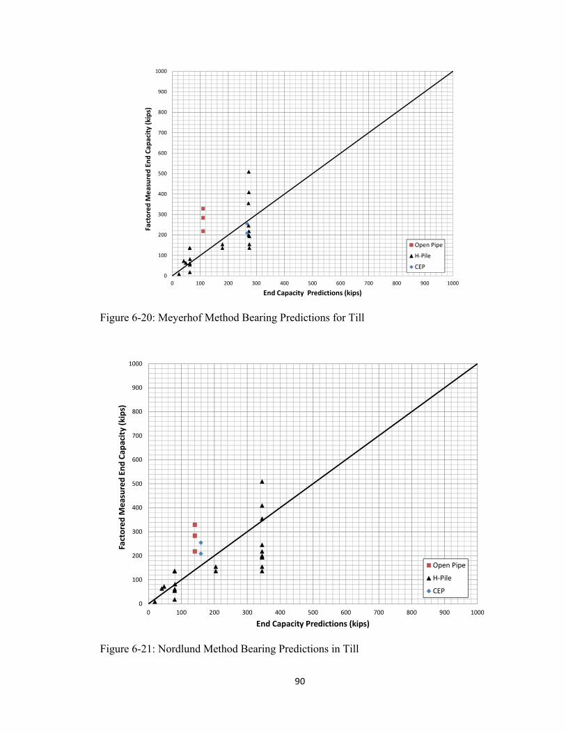
90
Figure 6-20: Meyerhof Method Bearing Predictions for Till
Figure 6-21: Nordlund Method Bearing Predictions in Till
!"##
$
%$$
&$$
'$$
($$
)$$
*$$
"$$
!$$
+$$
%$$$
$ %$$ &$$ '$$ ($$ )$$ *$$ "$$ !$$ +$$ %$$$
!"#$%&'(
)*'"+,&'()-.
()/"
0"#1$2)3410+5
-.()/"0"#1$2))6&'(1#$1%.+)3410+5
,-./#01-.
23014.
560
#
Figure 6-20: Meyerhof Method Bearing Predictions for Till
#
$
%$$
&$$
'$$
($$
)$$
*$$
"$$
!$$
+$$
%$$$
$ %$$ &$$ '$$ ($$ )$$ *$$ "$$ !$$ +$$ %$$$
!"#$%&'(
)*'"+,&'()-.
()/"
0"#1$2)3410+5
-.()/"0"#1$2)6&'(1#$1%.+)3410+5
,-./#01-.
23014.
560
#
Figure 6-21: Nordlund Method Bearing Predictions in Till

91
Figure 6-22: Meyerhof SPT Method Bearing Predictions in Till
6.4. Reliability of Selected Methods
The purpose of this section is to present the selected methods which provided the
most accurate predictions in a format which allows for the reliability of these methods to
be evaluated. Figure 6-23 through Figure 6-26 show the relative and cumulative
frequencies of the predicted to factored measured capacity ratios (PFMCR). These figures
can be used to pick appropriate PFMCRs for a desired reliability. The combination of
Meyerhof method and α-method indicates that approximately 68% of the data falls
below a PFMCR of 1.2 with 56% of all data falling within a range of PFMCRs of 0.4 to
1.2. Overall, the data shows a fairly tight distribution centered around a PFMCR of 1.0
which indicates a good fit. It also shows few outliers as approximately only 4% of data
exceeds a PFMCR equal to 2.8.
!!""
#
$##
%##
&##
'##
(##
)##
*##
!##
+##
$###
# $## %## &## '## (## )## *## !## +## $###
!"#$%&'(
)*'"+,&'()-.
()/"
0"#1$2)34
10+5
-.()/"0"#1$2)6&'(1#$1%.+)3410+5
,-./"01-.
23014.
560
"
Figure 6-22: Meyerhof SPT Method Bearing Predictions in Till
"
6.4. Reliability of Selected Methods
The purpose of this section is to present the selected methods which provided the
most accurate predictions in a format which allows for the reliability of these methods to
be evaluated. Figure 6-23 through Figure 6-26 show the relative and cumulative
frequencies of the predicted to measured capacity ratios (PMCR). These figures can be
used to pick appropriate PMCRs for a desired reliability. The combination of Meyerhof
and Alpha Methods indicates that approximately 68% of the data falls below a PMCR of
1.2 with 56% of all data falling within a range of PMCRs of 0.4 to 1.2. Overall, the data
shows a fairly tight distribution centered around a PMCR of 1.0 which indicates a good
fit. It also shows few outliers as approximately only 4% of data exceeds a PMCR equal to
2.8.

92
The PFMCRs shown for the proposed IRM in
Figure 6-24 indicate a fairly normal distribution of the data. Approximately 41%
of the predictions fall within a range of PFMCRs from 0.8 to 1.2. Additionally,
approximately 90% of the data falls below a PFMCR equal to 2.0. The majority of the
outliers occur on the over-prediction side of the distribution; however, only less than 1%
of the data exceeds a PFMCR of 3.0. When comparing the proposed IRM to the CGS
method (Figure 6-25), it is evident the CGS method predictions have a more poorly
distributed data set. The CGS method histogram does not show any significant peak in
the data shows a significant amount of outliers with approximately 48% of the data
falling below a PFMCR of 0.5 or above a ratio of 4.0.
The distribution of PFMCRs with Meyerhof method for end bearing till is shown
in Figure 6-26. The distribution indicates the existence of two distinct peaks in the data at
PFMCRs from 0.4 to 0.6 and 1.0 to 1.2; however, they are fairly close to one another
given the distribution of the remaining data. Approximately 54% of the data falls within
the PFMCR range of 0.4 to 1.2. Only 8% of the data lies above a PFMCR of 2.2 while
only 4% of the data lies above a PFMCR of 3.0. This indicates that the outliers are fairly
well contained, especially when compared to the CGS method results.
A brief statistical analysis of the data which indicates the appropriate PFMCR and
the corresponding confidence level for each method is shown in Table 6-7. A PFMCR for
each method was selected as the 95th percentile value for each data set i.e. 5% of piles
will have a PFMCR greater than the selected value. The 95% confidence interval
indicates what percentage of piles is likely to be observed below this PFMCR when used

93
in the future. It should be noted that a confidence interval could not be generated for the
Meyerhof method for bearing capacity in till because of the small sample size of data
included in the analysis. The PFMCR observed for this method still has 5% of piles
exceeding the value; however, its reliability cannot be confidently reported for future
projects. The PFMCR for the CGS method at the 95th percentile is very large indicating
the poor predictive ability of this method.
Figure 6-23: Reliability of Meyerhof Method and α-Method Combined Predictions for
Side Capacity
!"##
Meyerhof Method for bearing capacity in till because of the small sample size of data
included in the analysis. The PMCR observed for this method still has 5% of piles
exceeding the value; however, its reliability cannot be confidently reported for future
projects. The PMCR for the CGS Method at the 95th percentile is very large indicating
the poor predictive ability of this method.
"
"$%
"$&
"$'
"$(
)
"
"$)
"$%
"$*
"$&
"$+
","$& "$&,"$( "$(,)$% )$%,)$' )$',% %,%$& %$&,%$( %$(,*$% *$%,*$' *$',& -&
!"#"$%&'()*+,)-
")./0
1)$%&'(
)*+,)-")./0*2
3*4'$)
5*'.*1%
.6)
1%.6)*23*4,)7'/&)78+%/&2,)7*9)%5",)7*:'7)*!%;%/'&0#
Figure 6-23: Reliability of Meyerhof and Alpha Method Combined Predictions for Side
Capacity
#
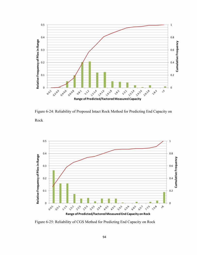
94
Figure 6-24: Reliability of Proposed Intact Rock Method for Predicting End Capacity on
Rock
Figure 6-25: Reliability of CGS Method for Predicting End Capacity on Rock
!"##
$
$%&
$%'
$%(
$%)
"
$
$%"
$%&
$%*
$%'
$%+
!"#"$%&'()*+,)-
")./0
1)$%&'(
)*+,)-")./0*2
3*4'$)
5*'.*1%
.6)
1%.6)*23*4,)7'/&)78+%/&2,)7*9)%5",)7*!%:%/'&0 #
Figure 6-24: Reliability of Intact Rock Method for Predicting End Capacity on Rock
#
#
$
$%&
$%'
$%(
$%)
"
$
$%"
$%&
$%*
$%'
$%+
!"#"$%&'()*+,)-
")./0
1)$%&'(
)*+,)-")./0*2
3*4'$)
5*'.*1%
.6)
1%.6)*23*4,)7'/&)78+%/&2,)7*9)%5",)7*;.7*!%:%/'&0*2.*12/< #
Figure 6-25: Reliability of CGS Method for Predicting End Capacity on Rock

95
Figure 6-26: Reliability of Meyerhof Method for Predicting End Capacity in Till
Table 6-7: Ratio of Predicted/Factored Measured Capacity at 95th Percentile with
Confidence Intervals
95% Confidence Interval
Method Predicted/Measured Lower Bound
Upper Interval
Meyerhof + α -‐Method for Side Capacity
2.52 90.7% 97.9%
Meyerhof Method for End Bearing in Till
2.48 N/A N/A
CGS Method for End Bearing on Rock
10.71 91.5% 98.0%
IRM for End Bearing on Rock
2.21 91.7% 97.8%
!"##
$
$%"
$%&
$%'
$%(
)
$
$%$*
$%)
$%)*
$%"
$%"*
!"#"$%&'()*+"#
,)-*.
/*0'$)
1
+"#
,)-*.
/*0'$)
1*'2*3%
24)
3%24)*./*0-)5'6&)578%6&.-)5*9)%1"-)5*!%:%6'&;#
Figure 6-26: Reliability of Meyerhof Method for Predicting End Capacity in Till
Table 6-7: Ratio of Predicted/Measured Capacity at 95th Percentile with Confidence
Intervals
** <=>*!.2/'5)26)*?2&)-(%$*
9)&@.5* 0-)5'6&)579)%1"-)5* A.B)-*C."25*
D::)-*?2&)-(%$*
+,-,./01#2#345/6#+,7/08#10.#9:8,#;656<:7-#
"%*"# !$%=># !=%!>#
+,-,./01#+,7/08#10.#?@8#A,6.:@B#:@#C:44#
"%&(# DE3# DE3#
;F9#+,7/08#10.#?@8#A,6.:@B#0@#G0<H#
)$%=)# !)%*># !(%$>#
IG+#10.#?@8#A,6.:@B#0@#G0<H#
"%")# !)%=># !=%(>#
96
Chapter 7:
SUMMARY AND CONCLUSIONS
7.1. Effectiveness of Pile Capacity Calculation Methods
The second phase of this study analyzed the effectiveness of static capacity
estimation methods recommended by the American Association of State Highway and
Transportation Officials (AASHTO) and Federal Highway Administration (FHWA) at
predicting Pile Dynamics, Inc. Case Pile Wave Analysis Program (CAPWAP®)
measured dynamic capacities at end of driving (EOD) and in some cases at the beginning
of restrike (BOR). For granular soils, the AASHTO recommended Nordlund method was
compared to Meyerhof’s soil property and Standard Penetration Test (SPT) based
methods. Both the α-method and β-methods, which are recognized by the FHWA and
AASHTO, were used to analyze cohesive soil layers. The Canadian Geotechnical Society
(CGS) method and the proposed Intact Rock method (IRM) were studied for piles
bearing on bedrock. For piles bearing in glacial till the Nordlund method was again
compared to Meyerhof’s soil property and SPT based methods.
7.1.1. Dynamic Measurements
It is important to note that the capacity of piles measured at the EOD will under-
estimate the long term capacity as capacity will increase when soil remolded during
driving recovers strength (setup). Piles can experience significant capacity increases with
time up to approximately one year after driving, especially if the pile is driven through
soft cohesive materials of considerable thickness. To compare the effectiveness of each
method, setup factors were needed to scale the CAPWAP® measured capacities to the
long term strength state (270 days). The setup factors were determined by using the Skov

97
and Denver (1988) relationship that had been calibrated to project piles that were tested at
both EOD and at BOR. The setup factors were found for cohesive and granular soil layers
separately. Furthermore, the cohesive factors were categorized by water content while the
granular setup factors were determined for low and high displacement piles separately. It
was shown in the calibration that the amount of setup in cohesive soil layers increased
with water content, while the setup in granular soil increased with the amount of soil
displaced by the pile. These setup factors were then applied to the dynamically measured
capacities for comparison to capacity estimates by the different methods. It should be
noted, however, that the majority of the restrike testing was conducted one day after
driving and the calibration found for this restrike was utilized to find setup to the long
term state at 270 days. Work by others on consolidation rates was utilized to estimate the
time required to achieve the 95% of the long term strength.
7.1.2. Pile Side Capacity
The side capacity predictions by each method were then compared to the factored
measured capacity for each pile analyzed. The factored measured capacities were plotted
against the prediction methods. All of the methods showed some significant scatter which
were often caused by anomalies in the subsurface or driving system. When justified,
these measurements were excluded from the side capacity analyses. One cause of these
low measurements is believed to be caused by soil arching around the pile in fill material
or loose overburden during driving which prevented the layer from contributing to the
measured capacity. Although downdrag and lateral squeeze may be present in the soft
clay when these granular soils overlay soft clays and may affect the strength of the clay,
the CAPWAP® method under the blow of the hammer should not detect downdrag. It is

98
more likely that the low factored strength of this soft clay may be caused by a low setup
factor. There were also some piles which were excluded from the analysis due to
apparent errors in the dynamic readings. These errors were evident due to significant and
suspected impossible changes in pile capacity from EOD to 1 day BOR. Additionally,
some data was excluded from the analysis due to an inadequate hammer to mobilize the
full pile capacity along the bottom of the pile. This was especially evident for some of the
piles tested at BOR where the setup along the pile caused the initial driving hammer to be
inadequate for BOR.
The side capacity comparisons indicated that the α-method predictions produced
more reliable estimates in cohesive soils than the β-method. In every case the granular
prediction method coupled with the α-method for cohesive resulted in better capacity
predictions than the granular prediction method coupled with the β-method for cohesive.
The results also indicated that the Meyerhof method was most reliable in predicting the
resistance of the granular soil layers. The Nordlund method for granular soils performed
the worst of all the prediction methods for granular soils. The comparisons using the
Nordlund method showed considerably more scatter than the other methods for granular
and had best fit lines for the measured versus predicted data that had significant
deviations from the equality line. Meyerhof’s method for granular material coupled with
the α-method for cohesive soils proved to be the most effective method for predicting
side capacity. The best fit line for the measured versus predicted capacities was nearly
unity and showed significantly less scatter than the other methods. The Nordlund method
for granular soils coupled with the β-method for cohesive soils performed the worst of all
side capacity measures. The Nordlund method and β-method predictions had

99
considerably more scatter than the other methods and significantly over-predicted the
measured pile capacities. The over-predictions of the Nordlund method for granular soils
were likely caused by the absence of a limiting factor with depth which both the
Meyerhof and Meyerhof SPT methods have for granular soils.
There were some limitations in the values of soil property evaluations that may
have contributed to the scatter in the side capacity predictions. The horizontal earth
pressure coefficients (Kh) used in the Meyerhof method for granular soils were taken
from typical published ranges and were not measured. This consideration is especially
relevant for the Kh values used in basal till as there are not published values available for
highly overconsolidated till. SPT results were corrected for type of hammer, diameter and
depth of borehole and the overburden pressure. The resulting STP (N1)60 was used in
correlations to obtain the peak drained friction angles for each soil layer. This is also
applicable to the Nordlund based methods as the friction angles used in this method were
also correlated from SPT N-values. These correlations have scatter and the direct
application to the glacial soils in Maine may incur further scatter. The SPT N-value can
be affected by large stress in the soil. The Meyerhof SPT method is susceptible to the
concerns of consistency in SPT readings since SPT corrections were not used at that time
and the N correlations by Meyerhof have large variability. Additionally, the friction angle
of 38° for tills found by tests for New Hampshire tills may not be representative for all
tills of varying particle size and composition. Shear strength of clay was primarily
obtained from vane shears that had a variety of configurations affecting strength. Better
estimates of these parameters could help improve side capacity predictions.
100
7.1.3. Pile End Bearing
7.1.3.1. Rock End Bearing
A new rock bearing method, the Intact Rock method (IRM), is proposed that
relates capacity to rock type in Maine. The proposed IRM and Canadian Geotechnical
Society (CGS) methods were compared to dynamic test results, and the results indicated
that the proposed IRM had significantly better predictions. The proposed IRM had less
scatter and had values closer to the line of unity than the CGS predictions. The cause of
the CGS method’s scatter is likely due to the uncertainty associated with its input
parameters. The limitations and causes of scatter for each of the methods are discussed
below.
The data available to designers from current subsurface investigations and
laboratory testing is too limited for the use of the CGS method. The CGS method requires
a detailed description of the entire bedrock mass beneath a project for piles bearing on
rock. Most parameters required as inputs for this method are not available from typical
subsurface investigations. Unconfined compressive strength (qu) of the bedrock is rarely
tested. Strengths based on a published range of values for each type of bedrock are then
utilized for this method. Detailed discontinuity information (e.g. joint spacing and
opening) is not directly available for the rock mass and must be interpolated from field
descriptions of discrete bedrock cores. Calculations performed by the MaineDOT were
included in the study where applicable. When the MaineDOT calculations were
unavailable, the input parameters for the CGS method were estimated from the bedrock
descriptions from each project’s boring logs. When neither was available, the CGS
method was not conducted for that pile. Ultimately the CGS method had a much larger

101
standard deviation and significantly more scatter than the piles analyzed using the
proposed IRM.
The proposed IRM uses back-calculated unconfined compressive strength of
bedrock to make estimations of end bearing capacity. The unconfined compressive
strengths were back-calculated from the measured CAPWAP® end bearing capacities and
contain average discontinuity effects and average rock strengths for Maine. The back-
calculated qu values for the proposed IRM were organized by bedrock type. The back-
calculated unconfined compressive strengths of sedimentary, igneous, and metamorphic
bedrock were 4.4, 5.4, and 5.2 ksi respectively. This process of back calculating strengths
was not effective for closed end pipe piles using the closed end area. The resulting qu for
these piles were significantly smaller than those calculated for the other pile types. To
account for this, a reduction factor of 9.3 was applied to the closed end pipe pile end area
to provide more reasonable predictions. The actual bearing area of the closed end pile
varies with the depth of penetration of the pile tip into the bedrock. This cross sectional
area is difficult to predict because bedrock hardness, quality, and strength are variable
from site to site, but after correction the area appears to be similar to H-piles and open
pipe pile steel area.
7.1.3.2. Till End Bearing
The Meyerhof method for estimating end bearing capacity in till resulted in the
best predictions. The Nordlund method showed very similar predictions to the Meyerhof
method. Both methods used the same assumed friction angle for all till of 38°, and the
Nordlund method specified by FHWA uses a Meyerhof limiting stress in its bearing
102
capacity estimations. The SPT method showed more scatter in its predictions which were
likely caused by the use of SPT readings from each subsurface investigation.
7.1.4. Reliability of Selected Static Capacity Methods
The best performing methods for the static capacity analysis of side capacity, end
bearing on rock and end bearing in till were the Meyerhof method and α-method
combined, the proposed IRM, and Meyerhof method respectively. The relative and
cumulative frequencies were plotted for each method and trends in the data were
highlighted. Additionally, the CGS method was investigated to highlight the poor
distribution and the amount of outliers which existed in the data.
A reliability analysis of each method was conducted which gave the predicted to
factored measured capacity ratio (PFMCR) corresponding to the 95th percentile of the
data. These PFMCRs were determined to be 2.52, 2.48, 10.72, and 2.21 for the Meyerhof
method and α-method combination for side capacity, Meyerhof end bearing in till, CGS
method for end bearing on rock and the proposed IRM for end bearing on rock
respectively. Additionally, a 95% confidence interval analysis was run for each method to
find the reliability of the 95th percentile value. It was found that generally the 95th
percentile PFMCR value may actually represent the 90th to 98th percentile value when
used in future analysis. The 95th percentile value could not be determined for the
Meyerhof method in till due to the small sample size available for analysis.

103
Chapter 8:
RECOMMENDATIONS
The following recommendations can be drawn from the conclusions of this paper to
help improve the pile design process for the MaineDOT.
The comparison of calculation methods to dynamic test capacities using information
provided by the subsurface reports and the dynamic test reports led to the following
recommendations.
1. The Meyerhof method for granular soils coupled with the α-method for cohesive
soils produced the most reliable results and are recommended for determining the
side shear resistances along driven piles.
2. The Meyerhof method for piles bearing in glacial till provided the most reliable
estimates and is recommended for determining the end bearing capacity of piles
not expected to reach bedrock.
3. It is recommended that for driven pile side capacity calculations the full cross
sectional area of the steel be used for open and closed end pipe piles and a box
area be assumed for H-piles (i.e. plugged flanges). For the end bearing on rock,
the enlarged bearing areas from the protective driving tips are recommended in
bearing capacity analyses for H-piles and open pipe piles. When calculating end
bearing on rock for closed end pipe piles, it is recommended that the full cross
sectional area of the pipe is used (a reduction factor of 9.3 is used in the
calculations).
4. The back-calculated average unconfined compressive strengths determined by
rock type or the use of site-specific unconfined compressive strength test results,

104
in conjunction with the proposed Intact Rock method (IRM) are recommended for
more reliable estimates of end bearing capacity on bedrock.
Most of the dynamic load tests were conducted only at the end of driving (EOD).
The EOD tests underestimate the long term capacity of piles. The following
recommendations cover the change of pile capacity with time after the EOD tests.
5. Setup factors are recommended to be applied to the EOD measured capacity to
determine a more representative pile capacity with time. Hannigan et al (2006)
recommend conducting restrike testing 2-6 days after EOD and ASTM D1143
recommends conducting a static load test 3-30 days after EOD. Initially, it is
recommended to apply 3 day setup values as determined in this study with a
resistance factor appropriate to the EOD measured capacity and with a separate
resistance factor appropriate to the added estimated setup capacity of the pile. If it
is possible, it is recommended that a restrike test in 3 days be used.
6. It is recommended to conduct beginning of restrike (BOR) tests to confirm the
setup of cohesive Maine soils with time. Some of the BOR tests are recommended
to be conducted at times when the cohesive soils are anticipated to be 95%
consolidated. These should be correlated to field exploration results.
Even the most reliable recommended methods had scatter of results in comparison
to dynamic load tests. Estimated subsurface stratigraphy and soil on rock property values
can contribute to the scatter. The following recommendations concern improvements in
soil/rock property values and stratigraphy that can lead to more reliable calculations.
105
7. At some abutments, there were significant differences in the measured capacity
and length of piles for different piles at the same abutment. Only one boring was
conducted at these abutments, but the pile load tests indicated changing
stratigraphy at the abutment. It is recommended that another boring be conducted
at abutments where the geologic investigations indicated possible stratigraphic
variations. The additional boring would improve the reliability of the calculated
capacity estimates.
8. Strength testing of glacial till is lacking in the literature. It is recommended that a
testing program be conducted to determine the strength characteristics for tills of
various compositions. The till should be obtained from at least two sites of
ablation till and two sites of basal till with each site having differing grain sizes.
Samples should be obtained from a test pit excavated by a backhoe, since
boreholes are inadequate to obtain representative till samples. Strength testing
should be conducted with triaxial equipment and large scale (to incorporate larger
particle sizes) direct shear equipment. This would lead to more reliability of the
calculated estimates for side friction and end bearing in the till layers.
9. The coefficient of friction, ϕ, for granular soils has been correlated to Standard
Penetration Test (SPT) N-values. Although this is the principal method of
obtaining ϕ, there are several correlations and the reliability of the correlations is
not known. It is recommended that a field and laboratory investigation be
conducted to determine the correlation of SPT N and ϕ values to obtain more
reliable estimates of side and end capacity in New England glacial granular
materials. This would require 3 borings per site with SPT each 3 ft. Test pits
106
would be excavated for samples and to obtain in situ densities. Triaxial test
equipment would be used to obtain strength values for various relative densities.
At least three non-till granular materials, each with a different grain size, as well
as one ablation till and one basal till should be sampled and tested.
10. For the Meyerhof method in granular, the lateral earth coefficient value (Kh) has
been taken from literature except for basal till where none was found. For basal
till where much of the side shear on piles appears to develop, the value of Kh
should be quite high as a result of the high over-consolidation. It is recommended
that data on the value of Kh, especially in basal till, be obtained by self-boring
pressuremeter field testing as an addition to Recommendation 9 to utilize the
results of Recommendation 9 sampling and testing. Pressuremeter boreholes
would be located in the vicinity of each SPT borehole. More than one basal till
location should be tested. This would lead to more reliability for the Meyerhof
method.
11. Although the proposed Intact Rock method (IRM) improves reliability compared
to the Canadian Geotechnical Society (CGS) method, there is still scatter with the
proposed IRM. It is recommended that site-specific uniaxial compressive strength
testing of intact rock be conducted for use in the proposed IRM. A LRFD
resistance factor of 0.50 is recommended to be applied to the nominal end bearing
pile resistance calculated using the proposed IRM.
12. When granular fill is placed over soft clay, then a hole may develop in the fill
around the pile during driving. The time for closing of the hole is variable. It is

107
recommended that no side support for the pile should be considered in the
granular fill in design calculations.
13. Once more data is obtained on soil and rock properties and setup; it is
recommended that resistance factors reflecting Maine’s conditions be formulated
for side and end bearing capacity of piles.
108
REFERENCES
AASHTO (2010). AASHTO LRFD Bridge Design Specifications. American Association of State Highway and Transportation Officials, Washington, D.C. AASHTO. (2002). Standard Specifications for Highway Bridges. 17th ed., Washington, D.C.: 2002. American Petroleum Institute. (1993). “Recommended practice for planning, designing and constructing fixed offshore platforms-working stress design.” API RP 2A, 20th Ed, American Petroleum Institute, Washington, D.C. Andrews, David W. (1987). "The Engineering Aspects Of The Presumpscot Formation." Proceedings of Geologic and Geotechnical Characteristics of the Presumpscot Formation Maine's Glaciomarine "Clay." Maine Geological Survey, Morrison Geotechnical Engineering, University of Maine Civil Engineering Dept., University of Southern Maine Geosciences Dept., Augusta, ME, 1-15. Aoki, N., and Velloso, D.A. (1975). “An approximate method to estimate the bearing capacity of piles.” Proc., 5th Pan-American Conference of Soil Mechanics and Foundation Engineering, Buenos Aires, 367-376. Associated Pile & Fitting (2012). Request for Information. 27 August 2012. Email. ASTM. (2008). "ASTM Standard 4945: Standard Test Method for High-Strain Dynamic Testing of Deep Foundations." ASTM International, West Conshohocken, PA. ASTM . (1996). " ASTM Standard 1143: Standard Test Method for Piles Under Static Axial Compression Load." ASTM International, West Conshohocken, PA. Attwooll, William J., Holloway, D. Michael, Rollins, Kyle M., Esrig, Melvin I., Sakhai, Si, and Hemenway, Dan. (1999). "Measured Pile Setup During Load Testing and Production Piling: I-15 Corridor Reconstruction Project in Salt Lake City, Utah." Transportation Research Record, Transportation Research Board, (1663), 1-7. Berezantzev, V. G., Khristoforov, V., and Golubkov, V. (1961). “Load Bearing Capacity and Deformation of Piled Foundations.” Proc. 5th Int. Conf. S.M. & F.E., vol. 2: 11-15. Bieniawski, Z.T. (1989). Engineering Rock Mass Classification, Wiley, New York, NY. Bjerrum, L. (1954). “Geotechnical properties of Norwegian marine clays,” Geotechnique., vol. IV, no. 2, pp 49-69. Bowles, J. E. (1977, 1982, 1988), Foundation Analysis and Design, McGraw-Hill, 816 pp.

109
Bradshaw, Aaron S., and Baxter, Christopher D. (2006). "Chapter 4. Dynamic And Static Pile Load Test Data - Design and Construction of Driven Pile Foundations: Lessons Learned on the Central Artery/Tunnel Project." Federal Highway Administration, <http://www.fhwa.dot.gov/engineering/geotech/pubs/05159/chapter4.cfm> (Apr. 29, 2012). Bullock, Paul J. (2012). Advantages of Dynamic Pile Testing. Full-scale Testing and Foundation Design: Honoring Bengt H. Fellenius. American Society of Civil Engineers, Reston, VA, 194-709. Caldwell, D. Q., Hanson, L.S., and Thompson, W.B. (1985). "Styles of Deglaciation in Central Maine." Late Pleistocene History of Northeastern New England and Adjacent Quebec. Geological Society of America, Boulder, CO, 45-58. Camp III, William M., and Parmar, Harpal S. (1999). "Characterization of Pile Capacity with Time in the Cooper Marl Study of Applicability of a Past Approach To Predict Long-Term Capacity." Transportation Research Record, Transportation Research Board, (1663), 16-24. Canadian Foundation Engineering Manual, 2nd ed., Canadian Geotechnical Society, Ottawa, Canada, pp. 456. (1985). Carter, J.P., and Kulhawy, F.H. (1988) “Analysis and Design of Drilled Shaft Foundations Socketed into Rock,” Report EL-5918, Electric Power Research Institute, Palo Alto, CA, 188. Das, Braja M. (2010). Principles of Foundation Engineering. Stanford, CT, Cengage Learning. Davisson, M.T. (1972). "High-Capacity Piles." Proceedings of Lecture Series on Innovations in Foundation Construction, Chicago, IL, 81-112. Dixon, Leif A. (1988). Effects of Bitumen Coating on the Axial and Lateral Loadings of Abutment Piles Subject to Downdrag. (Master’s Thesis). University of Maine, Orono, ME. Federal Highway Administration. (1990). “Dynamic Pile Monitoring and Pile Load Test Report: State Highway 77 Fore River Bridge Replacement.” Federal Highway Administration, Washington, D.C. Foye, K. C., Abou-Jaoude G. G., and Salgado R. (2004). Limit States Design (LSD) for Shallow and Deep Foundations. FHWA/IN/JTRP-2004/21. Joint Transportation Research Program, Indiana Department of Transportation and Purdue University, West Lafayette, Indiana.
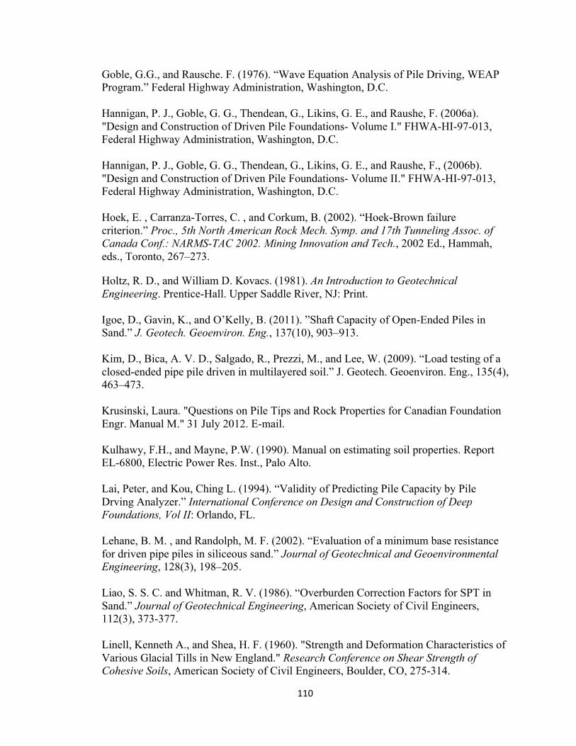
110
Goble, G.G., and Rausche. F. (1976). “Wave Equation Analysis of Pile Driving, WEAP Program.” Federal Highway Administration, Washington, D.C. Hannigan, P. J., Goble, G. G., Thendean, G., Likins, G. E., and Raushe, F. (2006a). "Design and Construction of Driven Pile Foundations- Volume I." FHWA-HI-97-013, Federal Highway Administration, Washington, D.C. Hannigan, P. J., Goble, G. G., Thendean, G., Likins, G. E., and Raushe, F., (2006b). "Design and Construction of Driven Pile Foundations- Volume II." FHWA-HI-97-013, Federal Highway Administration, Washington, D.C. Hoek, E. , Carranza-Torres, C. , and Corkum, B. (2002). “Hoek-Brown failure criterion.” Proc., 5th North American Rock Mech. Symp. and 17th Tunneling Assoc. of Canada Conf.: NARMS-TAC 2002. Mining Innovation and Tech., 2002 Ed., Hammah, eds., Toronto, 267–273.
Holtz, R. D., and William D. Kovacs. (1981). An Introduction to Geotechnical Engineering. Prentice-Hall. Upper Saddle River, NJ: Print. Igoe, D., Gavin, K., and O’Kelly, B. (2011). ”Shaft Capacity of Open-Ended Piles in Sand.” J. Geotech. Geoenviron. Eng., 137(10), 903–913. Kim, D., Bica, A. V. D., Salgado, R., Prezzi, M., and Lee, W. (2009). “Load testing of a closed-ended pipe pile driven in multilayered soil.” J. Geotech. Geoenviron. Eng., 135(4), 463–473. Krusinski, Laura. "Questions on Pile Tips and Rock Properties for Canadian Foundation Engr. Manual M." 31 July 2012. E-mail. Kulhawy, F.H., and Mayne, P.W. (1990). Manual on estimating soil properties. Report EL-6800, Electric Power Res. Inst., Palo Alto. Lai, Peter, and Kou, Ching L. (1994). “Validity of Predicting Pile Capacity by Pile Drving Analyzer.” International Conference on Design and Construction of Deep Foundations, Vol II: Orlando, FL. Lehane, B. M. , and Randolph, M. F. (2002). “Evaluation of a minimum base resistance for driven pipe piles in siliceous sand.” Journal of Geotechnical and Geoenvironmental Engineering, 128(3), 198–205. Liao, S. S. C. and Whitman, R. V. (1986). “Overburden Correction Factors for SPT in Sand.” Journal of Geotechnical Engineering, American Society of Civil Engineers, 112(3), 373-377. Linell, Kenneth A., and Shea, H. F. (1960). "Strength and Deformation Characteristics of Various Glacial Tills in New England." Research Conference on Shear Strength of Cohesive Soils, American Society of Civil Engineers, Boulder, CO, 275-314.

111
Long, James H., Bozkurt, Diyar, Kerrigan, John A., and Wysockey, Michael H. (1999). "Value of Methods for Predicting Axial Pile Capacity." Transportation Research Record, Transportation Research Board, (1663), 57-63. Long, J., Kerrigan, J., and Wysockey, M. (1999). "Measured Time Effects for Axial Capacity of Driven Piling." Transportation Research Record, Transportation Research Board, (1663), 8-15. Maine Department of Conservation. (2005). "Surficial Geologic History of Maine." Maine Geological Survey: Surficial Geology of Maine. <http://www.maine.gov/doc/nrimc/mgs/explore/surficial/facts/surficial.htm> (Sept., 13 2012). Maine Department of Conservation. (2005). "Maine Geological Survey: Fossils Preserved in Maine Sediments - Marine Limit." Maine Geological Survey: Fossils Preserved in Maine Sediments - Marine Limit. <http://www.maine.gov/doc/nrimc/mgs/explore/fossils/sediment/marine-limit.htm>. (Sept., 13 2012). Meyerhof, G.G. (1957). “Discussion on Research on Determining the Density of Sands by Spoon Penetration Testing.” Proceedings, Fourth International Conference on Soil Mechanics and Foundation Engineering, London, 3, 110. Meyerhof, G.G. (1976). “Bearing Capacity and Settlement of Pile Foundations.” Journal of the Geotechnical Engineering Division, American Society of Civil Engineers, 102 (GT3), 195-228. Navfac. (1986). DM-7.01 Soil Mechanics, Dept of Navy. Navfac. (1986). DM-7.02 Foundations & Earth Structures, Dept of Navy. Nordlund, R.L. (1963). “Bearing Capacity of Piles in Cohesionless Soils.” Journal of the Soil Mechanics and Foundations Division, ASCE, SM3, 1-35. Orrje, O. and Broms, B. B. (1967), "Effects of Pile Driving on Soil Properties." Journal of Soil Mechanics and Foundations Division, ASCE, 93 (SM5), 59-73. Paik, K. H. , and Salgado, R. (2003). “Determination of the bearing capacity of open-ended piles in sand.” J. Geotech. Geoenviron. Eng., 129 (1), 46-57. Paik, K. , Salgado, R. , Lee, J. , and Kim, B. (2003). “Behavior of open- and closed-ended piles driven into sands.” J. Geotech. Geoenviron. Eng., 129 (4), 296–306. Poulos, H. G., and E. H. Davis. (1980).Pile Foundation Analysis and Design. Wiley, New York.

112
Raushe, F., Thendean, G., Abou-Matar, H., Likens, G. E., and Goble, G. G. (1997). "Determination of Pile Driveability and Capacity From Penetration Tests, Volume I: Final Report.” FHWA-RD-96-179, Federal Highway Administration, McLean, VA. Raushe, F., Thendean, G., Abou-Matar, H., Likens, G. E., and Goble, G. G. (1997). "Determination of Pile Driveability and Capacity From Penetration Tests, Volume II: Appendixes.” FHWA-RD-96-180, Federal Highway Administration, McLean, VA. Raushe, F., Thendean, G., Abou-Matar, H., Likens, G. E., and Goble, G. G. (1997). "Determination of Pile Driveability and Capacity From Penetration Tests, Volume III: Literature Review, Data Base, and Appendixes.” FHWA-RD-96-181, Federal Highway Administration, McLean, VA. Rowe, R.K., and Armitage, H.H. (1987). “A Design Method for Drilled Piers in Soft Rock,” Canadian Geotechnical Journal, Vol. 24, pp. 126-142. R.W. Conklin Steel Supply. “HPile_Points.” RW Conklin Steel, <http://www.conklinsteel.com/images/HPile_Points.pdf> (Mar. 11, 2013). Sandford, Thomas C. (1989). “Evaluation of Dragdown on Pile,” University of Maine Civil Engineering Department, Report GT 89-2, April 1989, pp. 55. Sandford, Thomas C, and Amos, Jeannine. (1987). "Engineering Analysis of Gorham Landslide." Proceedings of Geologic and Geotechnical Characteristics of the Presumpscot Formation Maine's Glaciomarine "Clay." Maine Geological Survey, Morrison Geotechnical Engineering, University of Maine Civil Engineering Dept., University of Southern Maine Geosciences Dept., Augusta, ME, 1-28. Schnitker, D., and Borns, H. W. (1987). "Depositional Environmental and Composition of the Presumpscot Formation." Proceedings of Geologic and Geotechnical Characteristics of the Presumpscot Formation Maine's Glaciomarine "Clay." Maine Geological Survey, Morrison Geotechnical Engineering, University of Maine Civil Engineering Dept., University of Southern Maine Geosciences Dept., Augusta, ME, 1-13. Seo, H., Irem, Z.Y., and Prezzi, M. (2009). “Assessment of the axial load response of an H pile driven in multilayered soil.” J. Geotech. Geoenviron. Eng., 135(12), 1789-1804. Skov R, and Denver H. (1988). “Time-Dependence of Bearing Capacity of Piles.” Proceedings 3rd International Conference on Application of Stress-Waves to Piles, 1-10. Smith, Geoffrey W. (1985). "Chronology of Late Wisconsinan Deglaciation of Coastal Maine." Late Pleistocene History of Northeastern New England and Adjacent Quebec. Geological Society of America, Boulder, CO, 29-44. Sowers, G. F. (1979). "Chapter 11, Deep Foundations." Introductory Soil Mechanics and Foundations, Macmillan, 505-568.

113
Svinkin, M.R., and Skov, R. (2002). “Setup effect of cohesive soils in pile capacity.” Vulcan Hammer.net, <http://www.vulcanhammer.net/svinkin/set.php> (Mar. 4, 2013) Terzaghi, Karl, Ralph B. Peck, and Gholamreza Mesri. (1996). Soil Mechanics in Engineering Practice. Wiley, New York. Print. Thompson, Woodrow B. (1987)."The Presumpscot Formation in Southwestern Maine." Proceedings of Geologic and Geotechnical Characteristics of the Presumpscot Formation Maine's Glaciomarine "Clay," Maine Geological Survey, Morrison Geotechnical Engineering, University of Maine Civil Engineering Dept., University of Southern Maine Geosciences Dept., Augusta, ME, 1-22. Thurman, A.G. (1964). “Discussion of Bearing Capacity of Piles in Cohesionless Soils.” Journal of the Soil Mechanics and Foundations Division, American Society of Civil Engineers, SM1, 127-129. Tomlinson, M. J. (1957). "The Adhesion of Piles Driven in Clay Soils," Proc 4th Int Conf on Soil Mech and Found Eng, v 2, pp.66-71. Turner, John P. (2006). “Rock-socketed Shafts for Highway Structure Foundations.” NCHRP Synthesis 360, Transportation Research Board, Washington, D.C. Vesic, A. S. (1967). "A Study of Bearing Capacity of Deep Foundations," Final Rep., Proj. B-189,School of Civil Eng, Georgia Inst Tech.,Atlanta, Ga. Vijayvergiya, V.N., and Focht, J.A., Jr. (1972). A New Way to Predict Capacity of Piles in Clay, Offshore Technology Conference Paper 1718, Fourth Offshore Technology Conference, Houston. Wyllie, D.C. (1999). Foundations on Rock, 2nd ed., E&FN Spon, New York, N.Y., 401.

114
APPENDIX A: PILE TIP PROTECTION
Figure A-1: Pile Tip Protection for Open End Pipe Piles (APF 2012)

115
Figure A-2: Driving Tip Dimensions for Closed End Pipe Piles (APF 2012)

116
Figure A-3: Driving Tip Dimensions for H-Piles (R.W. Conklin Steel Supply 2013)

117
APPENDIX B: PRESENTATION OF DYNAMIC TEST DATA
0
200
400
600
800
1000
1200
1400
1600
1800
2000
0 20 40 60 80 100 120 140 160 180
Total C
apacity
(kips)
Depth of Penetration (feet)
H-‐Pile
Pipe Closed
Pipe Open
Figure B-1: Total Capacity of Piles on Bedrock
0
200
400
600
800
1000
1200
1400
1600
1800
2000
0 20 40 60 80 100 120 140 160 180
Total C
apacity
(kips)
Depth of Penetration (feet)
EOD -‐ H-‐pile, Pipe Open
BOR -‐ H-‐pile, Pipe Open
EOD -‐ Pipe Closed
Figure B-2: Total Capacity for Piles Bearing in Till
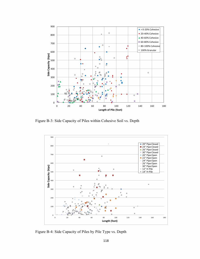
118
0
100
200
300
400
500
600
700
800
900
0 20 40 60 80 100 120 140 160 180
Side
Capacity
(kips)
Length of Pile (feet)
> 0-‐20% Cohesive
20-‐40% Cohesive
40-‐60% Cohesive
60-‐80% Cohesive
80-‐100% Cohesive
100% Granular
Figure B-3: Side Capacity of Piles within Cohesive Soil vs. Depth
0
100
200
300
400
500
600
700
800
900
0 20 40 60 80 100 120 140 160 180
Side
Capacity
(kips)
Length (feet)
20" Pipe Closed24" Pipe Closed26" Pipe Closed30" Pipe Closed20" Pipe Open22" Pipe Open24" Pipe Open26" Pipe Open30" Pipe Open12" H-‐Pile14" H-‐Pile
Figure B-4: Side Capacity of Piles by Pile Type vs. Depth
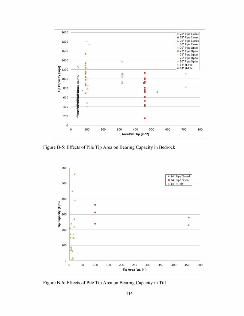
119
0
200
400
600
800
1000
1200
1400
1600
1800
2000
0 100 200 300 400 500 600 700 800
Tip Capacity (kips)
Area Pile Tip (in^2)
20" Pipe Closed24" Pipe Closed26" Pipe Closed30" Pipe Closed20" Pipe Open22" Pipe Open24" Pipe Open26" Pipe Open30" Pipe Open12" H-‐Pile14" H-‐Pile
Figure B-5: Effects of Pile Tip Area on Bearing Capacity in Bedrock
0
100
200
300
400
500
600
0 50 100 150 200 250 300 350 400 450 500
Tip Capacity (kips)
Tip Area (sq. in.)
24" Pipe Closed24" Pipe Open14" H-‐Pile
Figure B-6: Effects of Pile Tip Area on Bearing Capacity in Till
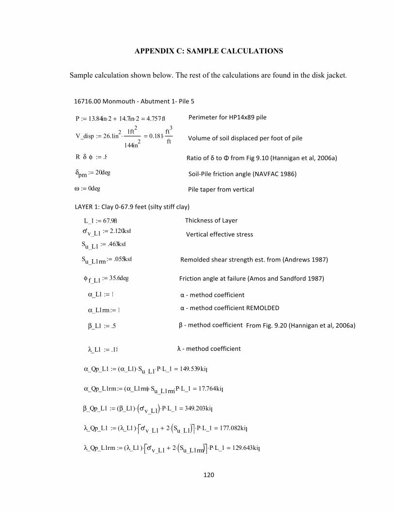
120
APPENDIX C: SAMPLE CALCULATIONS
Sample calculation shown below. The rest of the calculations are found in the disk jacket.
LAYER 1: Clay 0-‐67.9 feet (silty stiff clay)
Thickness of Layer
Vertical effective stress
Friction angle at failure (Amos and Sandford 1987)
α -‐ method coefficient
α -‐ method coefficient REMOLDED
β -‐ method coefficient From Fig. 9.20 (Hannigan et al, 2006a)
λ -‐ method coefficient
16716.00 Monmouth -‐ Abutment 1-‐ Pile 5
Perimeter for HP14x89 pile
Volume of soil displaced per foot of pile
Ratio of δ to Φ from Fig 9.10 (Hannigan et al, 2006a)
Soil-‐Pile friction angle (NAVFAC 1986)
Pile taper from vertical
Remolded shear strength est. from (Andrews 1987)
P 13.84in 2⋅ 14.7in 2⋅+ 4.757ft⋅=:=
V_disp 26.1in21ft2
144in2⋅ 0.181
ft3
ft⋅=:=
R_δ_φ .8:=
L_1 67.9ft:=
φ f_L1 35.6deg:=
α_L1 1:=
α_L1rm 1:=
β_L1 .51:=
λ_L1 .18:=
α_Qp_L1 α_L1( ) Su_L1⋅ P⋅ L_1⋅ 149.539kip⋅=:=
α_Qp_L1rm α_L1rm( ) Su_L1rm⋅ P⋅ L_1⋅ 17.764kip⋅=:=
β_Qp_L1 β_L1( ) σ'v_L1( )⋅ P⋅ L_1⋅ 349.203kip⋅=:=
λ_Qp_L1 λ_L1( ) σ'v_L1 2 Su_L1( )⋅+⎡⎣ ⎤⎦⋅ P⋅ L_1⋅ 177.082kip⋅=:=
λ_Qp_L1rm λ_L1( ) σ'v_L1 2 Su_L1rm( )⋅+⎡⎣ ⎤⎦⋅ P⋅ L_1⋅ 129.643kip⋅=:=
δpm 20deg:=
ω 0deg:=
σ'v_L1 2.120ksf:=
Su_L1 .463ksf:=
Su_L1rm .055ksf:=

121
LAYER 2: Granular Layer 67.9-‐105 feet
Thickness of Layer
Corrected SPT value for granular material
Friction angle at failure
Friction angle between soil and pile
Vertical effective stress
Meyerhof Limiting depth for Dr<30
Vertical effective stress when L>L'
Correction factor when δ does not equal ϕf log linear interpolation for Kδ factor in Nordlund method from Table 9-‐4a (Hanniganet al, 2006a)
K value for Meyerhof's Eq. from Kulhawy and Mayne (1990)
calculated is less than limiting value of 100 kPa (Hannigan et al, 2006a) so use calculated
LAYER 3: Till Layer 105-‐141 feet
Thickness of Layer
N1_60_L3 not provided for till layer Corrected SPT value for granular material
Friction angle at failure
Friction angle between soil and pile
Vertical effective stress
Limiting depth for Dr<30
L_2 105ft 67.9ft− 37.1 ft⋅=:=
N1_60_L2 7.9:=
φ f_L2 30.5deg:=
δp R_δ_φ( ) φ f_L2( )⋅ 24.4 deg⋅=:=
σ'v_L2 5.327ksf:=
L' 101412ft⋅ 11.667ft⋅=:=
σ'v_L' .729ksf:=
CF_L2 .9:=
Kδ_L2 10
log .88( ) log 1.135( )−
log .1( ) log .2( )−log .1( ) log .181( )−( )⋅ log .88( )−⎡⎢
⎣⎤⎥⎦
−1.094=:=
Ko_L2 .495 1.75⋅ 0.866=:=
Nordlund_Qp_L2 Kδ_L2( ) CF_L2( )⋅ σ'v_L2( )⋅sin δp ω+( )cos ω( )
⋅ P⋅ L_2⋅ 382.422kip⋅=:=
Meyerhof_SPT_qp_L2 N1_60_L2( ) 7.9=:= kPa
Meyerhof_SPT_QP_L2 Meyerhof_SPT_qp_L2 .029⋅ ksf P⋅ L_2⋅ 40.43kip⋅=:=
Meyerhof_Prop_Qp_L2 Ko_L2( ) σ'v_L'( )⋅ tan δpm( )⋅ P⋅ L_2⋅ 40.561kip⋅=:=
L_3 141ft 105ft− 36 ft⋅=:=
φ f_L3 38deg:=
δp R_δ_φ( ) φ f_L3( )⋅ 30.4 deg⋅=:=
σ'v_L3 7.756ksf:=
L' 101412ft⋅ 11.667ft⋅=:=
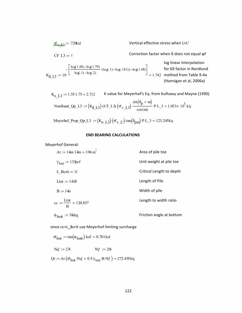
122
Vertical effective stress when L>L'
Correction factor when δ does not equal ϕf
log linear interpolation for Kδ factor in Nordlund method from Table 9-‐4a (Hannigan et al, 2006a)
K value for Meyerhof's Eq. from Kulhawy and Mayne (1990)
END BEARING CALCULATIONS
Meyerhof General:
Area of pile toe
Unit weight at pile toe
Critical Length to depth
Length of Pile
Width of pile
Length to width ratio
Friction angle at bottom
since cc>L_Bcrit use Meyerhof limiting surcharge
σ'v_L' .729ksf:=
CF_L3 .9:=
Kδ_L3 10
log 1.48( ) log 1.79( )−
log .1( ) log .2( )−log .1( ) log .181( )−( )⋅ log 1.48( )−⎡⎢
⎣⎤⎥⎦
−1.742=:=
Ko_L3 1.55 1.75⋅ 2.712=:=
Nordlund_Qp_L3 Kδ_L3( ) CF_L3( )⋅ σ'v_L3( )⋅sin δp ω+( )cos ω( )
⋅ P⋅ L_3⋅ 1.053 103× kip⋅=:=
Meyerhof_Prop_Qp_L3 Ko_L3( ) σ'v_L'( )⋅ tan δpm( )⋅ P⋅ L_3⋅ 123.245kip⋅=:=
At 14in 14⋅ in 196 in2⋅=:=
γ toe 135pcf:=
L_Bcrit 10:=
Ltot 141ft:=
B 14in:=
ccLtotB
120.857=:=
φbott 38deg:=
σ'bot tan φbott( ) ksf⋅ 0.781ksf⋅=:=
Nq' 230:= Nγ' 260:=
Qt At σ'bot Nq'⋅ 0.5 γ toe⋅ B⋅ Nγ'⋅+( )⋅ 272.455kip⋅=:=

123
coefficient
since calculated stress is > limiting stress of 3.2 ksf use:
use Qp
Meyerhof SPT from boring log
correction factor
Nordlund Method
Limiting value for sands
αt 0.72:=
Nq'nord 110:=
σ'v_bott 7.756ksf:=
σ'v_bott_lim 3.2ksf:=
Qp αt Nq'nord⋅ σ'v_bott_lim⋅ At⋅ 344.96kip⋅=:=
qL 265ksf:=
Qp_limit qL At⋅ 360.694kip⋅=:=
N60 50:=
CN1
σ'v_bott2000psf
⎛⎜⎝
⎞⎟⎠
⎡⎢⎢⎣
⎤⎥⎥⎦
0.50.508=:=
N1_60 N60 CN⋅ 25.39=:=
Qpspt At0.8N1_60⋅ L_3( )⋅
Bksf⋅
⎡⎢⎣
⎤⎥⎦
⋅ 853.111kip⋅=:=
QL 8 N1_60⋅ ksf⋅( ) At⋅ 276.471kip⋅=:=