Embed Size (px)
Citation preview

L e c t u r e - 7
Transportation Economics and Decision Making

Pricing and Subsidy Policies
One of the most difficult problems in transportation
Congestion of motor vehicles in urbanized areas
Congestion creates
Loss in private and societal cost
Higher operating cost
Losses in valuable time
More highway crashes
More air pollution
More discomfort, inconvenience
Noise pollution

What are the choices
Naturally, the society‟s choices are to
Do nothing
Reduce inconvenience by increasing capacity
Restrict road use to congested areas in the network
Long standing experience suggests that the first two choices further add congestion and leading to greater inefficiency
The third choice offers the possibility to solve the problem through prcing.

How pricing is considered
Three broad category of choices
Taxes on suburban or dispersed living‟
Subsidies to public transportation
Increased cost of driving including road and parking pricing
One of the important methods of reducing congestion is through taxing the motorist (congestion pricing)
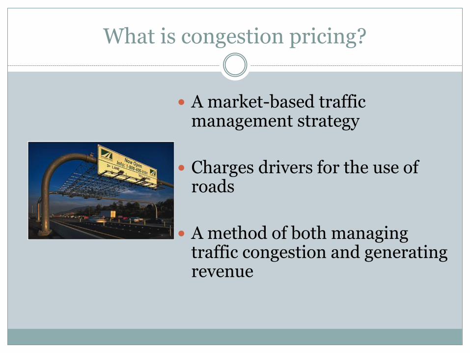
What is congestion pricing?
A market-based traffic management strategy
Charges drivers for the use of roads
A method of both managing traffic congestion and generating revenue

How Congestion Pricing Manages Congestion
Charges for use of congested areas during times of peak use provides an incentive for people who do not need to be on the road to postpone trips to non-peak hours or shift modes
These trips would be more efficient during off-peak hours

Types of Congestion Pricing
Cordon Pricing
London
Congestion Pricing in the U.S.?
FHWA funds available under SAFETEA-LU for implementing congestion pricing
Urban Partnership Agreements – U.S. Department of Transportation
Public-Private Partnership (PPP)
Benefits
Reduction of peak-period and total roadway congestion
Better mass transit
Reduction of greenhouse gas emissions and energy consumption
Increased traffic safety?

(Transportation Alternatives)
How it works

A Transport Network Model
v is the speed in km/h on the network.
q is number of vehicles = the traffic flow.
v(q) is the speed-flow relationship, v‟<0.
c is the travel cost per km of a representative vehicle: c(q)=a+b/v(q) a is “fixed” cost of travel per vehicle
b is cost per vehicle (including opportunity cost of time);
Total social cost is C(q)=c(q)q
The (inverse) demand (the marginal social benefit, MSB) of an extra vehicle on the network is D(q) with D‟<0.

Costs
qv
v
bdqdc
dqdC qqcqqcMSC
2)()(
)()()( qMPCqcqASCqC
Marginal social cost of an extra vehicle on the network:
Private marginal
cost
Marginal external
cost borne by other
users.
Reduction
in speed
Average social cost of an extra vehicle on the network:
Average Social Cost (ASC) = Marginal private cost (MPC)

Traffic Flows
Vehicles enter the network until the private marginal benefit is equal to the private marginal cost:
)()( aa qMPCqD
• The socially optimal number of vehicles entering the network is determined by:
)()( ee qMSCqD
)( aqASC
ea qqqASCqMSC )()(

Congestion Pricing
Traffic flow
Cost
s per
trip
D = MPB = MSB
MSC
ASC D
C
M
E
G
F
qe qa qf

Congestion Pricing (2)
qf is the free flow speed per hour and cost is lower than G
(includes time and operating expenses)
Beyond qf , speed falls, therefore cost per trip increases for each additional user
Additional vehicle increases the operating cost of all other vehicles in the stream of flow.

Congestion Pricing (3)
Pricing should be in accord with marginal cost to give rise to a flow equal to qe
This could be achieved by charging a toll of ED
Thus rising the average cost curve to achieve optimal traffic flow.

Congestion Pricing (4)
The benefit from this action is the reduction
operating cost of all the remaining vehicles and
the loss of benefit from the additional trips beyond optimal (qa-qe)

Optimal congestion charges
First-best corrective (Pigouvian) charge = MSC-MPC at traffic flow qe.
Levied directly on the congestion externality but should vary by link, junction and time.
“Electronic plate” that records where each vehicle is at any point in time and charge the owner accordingly.

Second best road prices
It is costly to collect charges that vary by link, junction and time => cannot tax the congestion externality directly.
How then to design an optimal second-best road pricing system?
Tax fuel? Fairly good proxy for road damage, but not for congestion.
Subsidise public transport? Costly to do, but bus lanes, raising bollards, bike paths can be seen as an attempt to shift the balance.
Use a cordon system to price congestion.

Congestion Pricing
The Federal Highway Administration has established the following relationship between travel time and flow on a 10 mile length of a highway
The demand function is given by d= 4000-100t The value of travel time of users is $8 per vehicle hour. What should be the congestion toll on this section of highway. Notations: t-> travel time (min) V-> flow (veh/hour) d->demand
𝑡 = 10 1 + 0.15𝑉
2000
4

Time taken by all the vehicles travelling this section
Let us form a table and plot results
𝑡𝑉 = 10 1 + 0.15𝑉
2000
4V
=10 𝑉 + 0.15𝑉
2000
5
Marginal time = 𝑑(𝑡𝑉)
𝑑𝑉= 10 1 + 0.75
𝑉
2000
4
Volume (veh/hr)
Time (min)
Demand D=4000-100t
Speed (mph)
Marginal Time (min)

Solution
0.00
10.00
20.00
30.00
40.00
50.00
60.00
1000 1500 2000 2500 3000
time Marginal Time
19.12
11.82
Toll = 19.12 – 11.82 = 7.3 min = 7.3*8/60=$0.97 Length of section = 10 miles Toll/mile = 9.7 cents
Solution (2)
Personal time is the average cost,
Average cost curve represents flow on highway when each trip-maker is only aware of his/her own personal time
The additional time of adding one extra vehicle to the traffic stream is referred as marginal time and is shown in marginal curve
(additional time is taken over the 10 mile span)
The intersection of demand curve and the marginal curve shows the optimal flow (2100 veh/hr)

Solution (3)
Optimal flow on the highway occurs when a trip is made only if benefit of a trip to the trip maker exceeds the additional time imposed on the trip maker
The differential cost of average and marginal cost would show what would be the pricing

Depreciation

Depreciation Concept
Common usage of depreciation is in the sense of decrease in value of a machine, property, etc.
A state of physical wear and tear
Replacement is higher than the amount of depreciation of the real estate.
Income generating property

Use of Depreciation
Calculating net operating profits, especially when profits are distributed to stock holders.
Estimating bid prices as does a contractor
Calculating production cost as a basis of price setting as is done in regulating of public utilities
Deciding property valuation for tax purposes, settlement of estates, including, determining the fair value rate base in utility regulations
Analyzing investment securities for their investment merit

Depreciation and Value
Used in the sense of decrease in value.
The lessening of value is a result of increasing age and obsolescence and decreasing usefulness of the property.
Man made physical properties generally do decrease in value with age and use as long as the general price level remains substantially stable.
Value of a property depends upon the economic laws of supply and demand, hence depreciation or appreciation both can occur.

Depreciation and Usefullness
Impaired service usefulness of physical property or the state of wear and tear
The intent is to give some indication of how the remaining service usefulness of a property compares to a similar or identical property that is new.
In this sense, there is no direct reference to the value of the property, although it is inferred that any property highly depreciated (in the physical sense) is probably worth considerably less than it would be were it new.

Methods of Allocating Depreciation Expense
Straight Line Method
Declining Balance Method
Double-Declining Balance Method
Sum of Digits Method
Sinking Fund Method
Present Worth Method

Notations
B = Depreciation base including terminal value
Bd = Depreciable base = B - T
Bx = Unallocated portion of Dep. Base yet unallocated at age X
T = Terminal value
B - Bx = Total depreciation at age X
D = Annual depreciation allocation

Notations (2)
Dx = Accumulated Dep. Allocation at age X
X= Age of the property
n = Probable service life
f = Depreciation rate per year
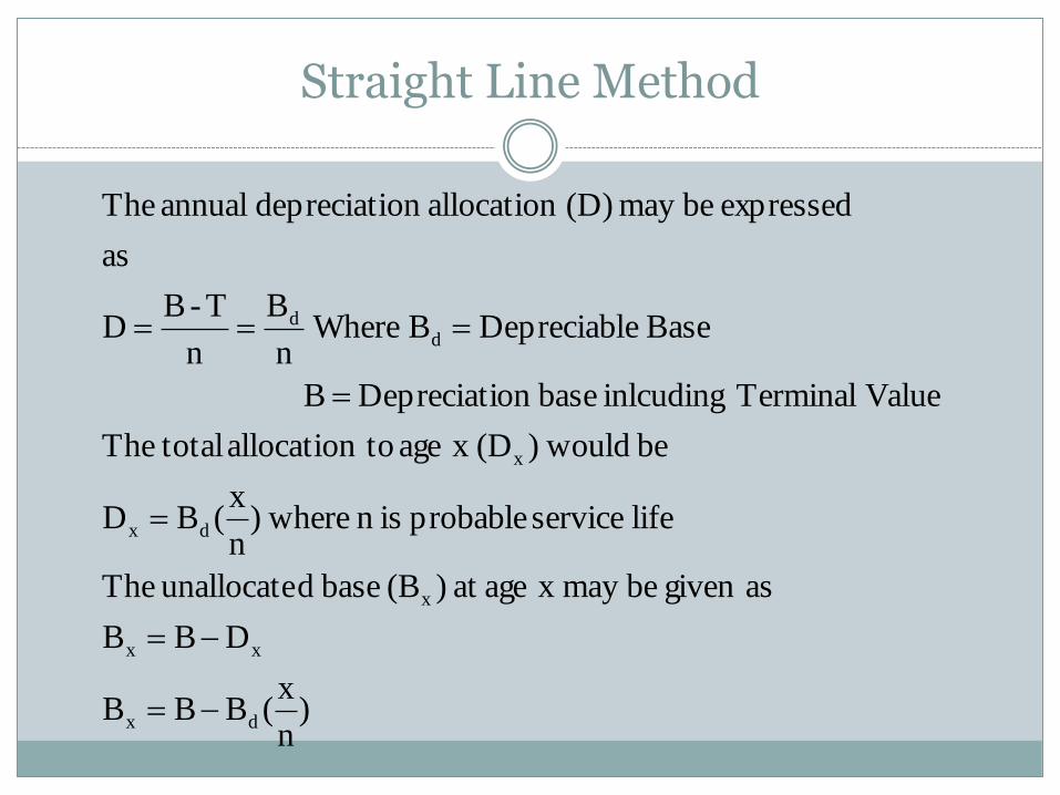
Straight Line Method
)n
x(BBB
DBB
asgiven bemay x ageat )(B base dunallocate The
life service probable isn where)n
x(BD
be would)(D x age toallocation totalThe
Value Terminal inlcuding baseon Depreciati B
Base eDepreciablB Wheren
B
n
T-BD
as
expressed bemay (D) allocationon depreciati annual The
dx
xx
x
dx
x
dd

Straight Line Method (2)
property of Age x
Value Terminal T
Base eDepreciablB
Baseon Depreciati ofportion ed UnallocatB Where
T)n
x-n(BB
T)n
x-(1BB
)n
x(BT)(BB
d
x
dx
dx
ddx

Straight Line Method-Example
Original Amount 50,000
Salvage Value 10,000
Time Period 5
Year D Bx B-Bx
0 50000 0
1 8000 42000 8000
2 8000 34000 16000
3 8000 26000 24000
4 8000 18000 32000
5 8000 10000 40000
0
10,000
20,000
30,000
40,000
50,000
60,000
0 1 2 3 4 5 6Un
allo
cate
d P
ort
ion
of
De
pre
ciat
ion
Time (Years)
SL
SL

Straight Line Method
Simple, easily applied method that distributes the depreciable base according to a positive system that requires the exercise of judgment only in estimating the service life and the terminal value
Has a long record of acceptance in industry and business

Declining Balance Method
In this method, a fixed percentage depreciation expense is used for each allocation period applied to the remaining, or unallocated, cost balance at the beginning of the period.

Declining Balance Method (2)
:n life probable
chosenany for computed be can f rate ondepreciati
the point, end at chosen is value terminal a When
zero
reach not willB the zero, than greater
andunity than less always is f)(1- factor the Since
f)B(1-B
by given is
base the to portion dunallocate the constant, is method
balance declining the in ondepreciati of rate the Since
x
x
x
x
base dunallocate
rate/year Dep. f base, Dep. B
Base Dep. ofportion ed UnallocatB Where x

Declining Balance Method (3)
n
n
B
T1f
rate/yr Dep. f Value, Terminal T
base Dep. B e, Wherf)-B(1T

Declining Balance Method-Example
Original Amount 50,000
Salvage Value 10,000
Time Period 5
Year D Bx B-Bx
0 50,000 0
1 13,761 36,239 13,761
2 9,974 26,265 23,735
3 7,229 19,037 30,963
4 5,239 13,797 36,203
5 3,797 10,000 40,000
0
10,000
20,000
30,000
40,000
50,000
60,000
0 1 2 3 4 5 6Un
allo
cate
d P
ort
ion
of
De
pre
ciat
ion
Time (Years)
DB
DB

Double Declining Balance Method
Depreciation rate, f= 2/n
Original Amount 50,000
Salvage Value 10,000
Time Period 5
Year D Bx B-Bx
0 50000 0
1 20000 30000 20000
2 12000 18000 32000
3 7200 10800 39200
4 800 10000 40000
5
0
10,000
20,000
30,000
40,000
50,000
60,000
0 1 2 3 4 5Un
allo
cate
d P
ort
ion
of
De
pre
ciat
ion
Time (Years)
DDB
DDB
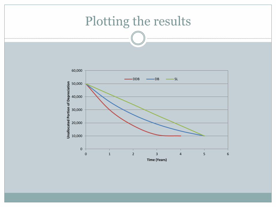
Plotting the results
0
10,000
20,000
30,000
40,000
50,000
60,000
0 1 2 3 4 5 6
Un
allo
cate
d P
ort
ion
of
De
pre
ciat
ion
Time (Years)
DDB DB SL

Sum of Years Digit Method
Sum of the digit method uses a definite method of calculating the depreciation rate
It gives decreasing annual depreciation each following year
The decreasing charges are obtained by the arithmetical concept used.
The depreciation rate is applied to the depreciable base, B-T
It is a scheme, which allocates the largest annual charge to the first year of service and the smallest to the last year.

Sum of Years Digit Method (2)
Original Amount 50,000
Salvage Value 10,000
Time Period 5
Year Factor Depreciation Bx B-Bx
0 0 50000 0
1 0.33 13,333.33 36,666.67 13333.33
2 0.27 10,666.67 26,000.00 24000
3 0.20 8,000.00 18,000.00 32000
4 0.13 5,333.33 12,666.67 37333.33
5 0.07 2,666.67 10,000.00 40000
0
10,000
20,000
30,000
40,000
50,000
60,000
0 1 2 3 4 5 6Un
allo
cate
d P
ort
ion
of
De
pre
ciat
ion
Time (Years)
SumOfYears
SumOfYears

Plotting the results (2)
0
10,000
20,000
30,000
40,000
50,000
60,000
0 1 2 3 4 5 6
Un
allo
cate
d P
ort
ion
of
De
pre
ciat
ion
Time (Years)
DDB DB SL SumOfYears

Sinking Fund Method
The method is based on the compound interest theory.
Bye the sinking fund theory, the equal annual year-end deposits in a sinking fund would accumulate with compound interest thereon to the total depreciation allocation to any given date.
The allocation for a specific year is, therefore, the annual deposit,or annuity, plus the compound interest increment to the fund for the year.

Sinking Fund Method (2) 47
Annual year end deposit to a fund to accumulate to “F” in „n‟ years at „i‟ interest rate is:
A = F i
(1+i)n - 1
A = (B - T) i
(1+i)n - 1
F = A (1+i)n - 1
i
The accumulation to any date n is given by

Sinking Fund Method (3) 48
In terms of depreciation symbols
Dx = A
(1+i)x - 1
i
Dx = (B - T)
i
(1+i)n - 1 [ ]
(1+i)x - 1
i [ ]
Dx = (B - T)
(1+i)n - 1 [ ]
(1+i)x - 1
Dx = Bd
(1+i)n - 1 [ ]
(1+i)x - 1

Sinking Fund Method (4) 49
Bx = (Bd + T) - Bd
(1+i)n - 1 [ ]
(1+i)x - 1
Bx = Bd (1+i)n - (1+i)x
(1+i)n - 1 + T [ ]
The unallocated base at age x would be then be given by

Sinking Fund Method-Example
Original Amount 50,000
Salvage Value 10,000
Time Period 5
Interest rate 5%
Year Factor Bx B-Bx
0.00 1.00 50,000.00 0.00
1.00 0.82 42,761.01 7,238.99
2.00 0.63 35,160.07 14,839.93
3.00 0.43 27,179.08 22,820.92
4.00 0.22 18,799.04 31,200.96
5.00 0.00 10,000.00 40,000.00
0
10,000
20,000
30,000
40,000
50,000
60,000
0.00 1.00 2.00 3.00 4.00 5.00 6.00Un
allo
cate
d P
ort
ion
of
De
pre
ciat
ion
Time (Years)
SinkingFund
SinkingFund
T1r)(1
r)(1r)(1BB
n
xn
dx
Depreciation Coefficient

Present Worth Method
Variant of the sinking fund method
The concept is that the decrease in the value of the property in any given year, and therefore its depreciation for the year, is equal to the decrease for that year in the present value of its probable future returns.
In terms of depreciation symbols and say rate of return „r‟ is analogous to „i‟ then the following can be written:
B = Bd + T
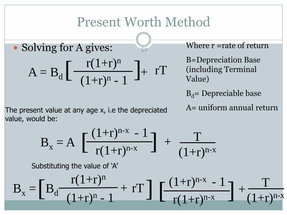
Present Worth Method
52 Solving for A gives:
r(1+r)n [ A = Bd
(1+r)n - 1 + ] rT
The present value at any age x, i.e the depreciated value, would be:
Bx = A T
(1+r)n-x
(1+r)n-x - 1
r(1+r)n-x [ ] +
Substituting the value of ‘A’
(1+r)n-x - 1
r(1+r)n-x [ ] r(1+r)n
Bx = Bd rT [ ] +
(1+r)n - 1
T
(1+r)n-x +
Where r =rate of return
B=Depreciation Base (including Terminal Value)
Bd= Depreciable base
A= uniform annual return

Present Worth Method
53 (1+r)n - (1 + r)x Bx = Bd T
[ ] + (1+r)n - 1
Capital Recovery Factor =
(1+r)n - 1
r(1+r)n
Where r =rate of return
Bx=Unallocated portion of depreciable Base at age x
Bd= Depreciable base (Depreciation base-Terminal value)
A= uniform annual return
Note that the formula for computing the depreciation using Sinking Fund Method and Present Worth Method is same except r (rate of return) is used in Sinking Fund Method instead of i (interest rate) in Present Worth Method.

Complete the Example with PW Method
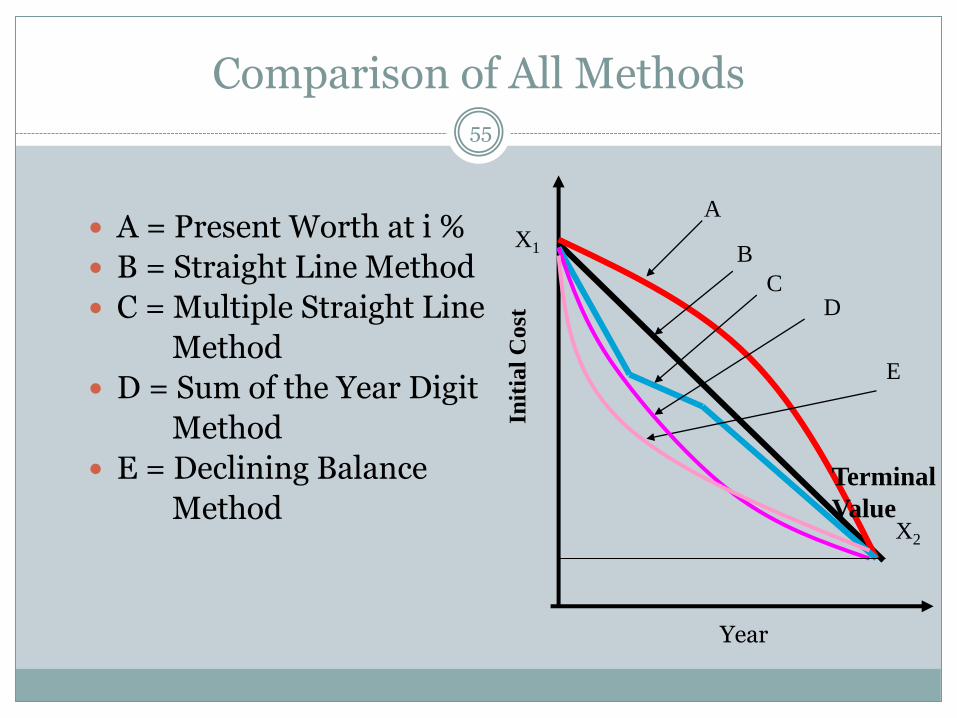
Comparison of All Methods 55
A = Present Worth at i %
B = Straight Line Method
C = Multiple Straight Line
Method
D = Sum of the Year Digit
Method
E = Declining Balance
Method
A
B
C D
E
X2
X1
Terminal
Value In
itia
l C
ost
Year