1

Transmit Power Pool Design for Grant-FreeNOMA-IoT Networks via Deep Reinforcement

LearningMuhammad Fayaz, Student Member, IEEE, Wenqiang Yi, Member, IEEE, Yuanwei Liu, Senior Member, IEEE,

and Arumugam Nallanathan, Fellow, IEEE,

Abstract—Grant-free non-orthogonal multiple access (GF-NOMA) is a potential multiple access framework for short-packet internet-of-things (IoT) networks to enhance connectivity.However, the resource allocation problem in GF-NOMA ischallenging due to the absence of closed-loop power control.We design a prototype of transmit power pool (PP) to provideopen-loop power control. IoT users acquire their transmit powerin advance from this prototype PP solely according to theircommunication distances. Firstly, a multi-agent deep Q-network(DQN) aided GF-NOMA algorithm is proposed to determinethe optimal transmit power levels for the prototype PP. Morespecifically, each IoT user acts as an agent and learns a policyby interacting with the wireless environment that guides themto select optimal actions. Secondly, to prevent the Q-learningmodel overestimation problem, double DQN (DDQN) based GF-NOMA algorithm is proposed. Numerical results confirm thatthe DDQN based algorithm finds out the optimal transmit powerlevels that form the PP. Comparing with the conventional onlinelearning approach, the proposed algorithm with the prototypePP converges faster under changing environments due to limitingthe action space based on previous learning. The considered GF-NOMA system outperforms the networks with fixed transmissionpower, namely all the users have the same transmit power andthe traditional GF with orthogonal multiple access techniques,in terms of throughput.

Index Terms—Double Q learning, Grant-free NOMA, Internetof things, Multi-agent deep reinforcement learning, Resourceallocation

I. INTRODUCTION

One of the main challenges to the next generation cellularnetworks is the provision of massive connectivity to explo-sively increased Internet-of-things (IoT) users, especially foruplink transmission. In current cellular networks, enablingmultiple access with limited resources is an inherent problem.Fortunately, non-orthogonal multiple access (NOMA) witha new degree of freedom, namely the power domain, hasbeen established as a promising technique for the solutionof this problem [2]. Some latest work investigating NOMAfrom different aspects can be found in [3] [4] [5]. Althoughgrant-based (GB) has been widely studied, it fails to providesufficient access to IoT users with short packets, since multiple

M. Fayaz, W. Yi, Y. Liu, and A. Nallanathan are with Queen MaryUniversity of London, London, UK (email:{m.fayaz, w.yi, yuanwei.liu,a.nallanathan}@qmul.ac.uk).

M. Fayaz is also with the Department of Computer Science and IT,University of Malakand, Pakistan.

Part of this work was submitted in IEEE International Conference onCommunications (ICC), June, Canada, 2021 [1].

handshakes are required before the transmission. Therefore,grant-free (GF) NOMA is proposed to enhance this connec-tivity.

In GF-NOMA, multiple IoT users transmit data in an arrive-and-go manner to the base station (BS) on the same time-frequency resource block (RB) without waiting for the BSto schedule and grant [6]. However, the resource allocationproblem in GF-NOMA is challenging as BSs commonly haveno/partial information about the active users and their channelstate information (CSI). Additionally, keeping enough powerdifference for successful successive interference cancellation(SIC) processes at the NOMA-enabled BS side is a toughpractical challenge. As NOMA is heavily based on the receivedpower difference among users [7], the effectiveness of sucha solution is limited for GF schemes in the absence of aclosed-loop power control [8]. It is worth noting that userclustering and power allocation in NOMA is mainly dependedupon their channel gain, which can be calculated via IoT usersgeographical information and practical statistic models. Suchinformation can be acquired without information exchanges,which enables an open loop. Therefore, a prototype of transmitpower pool for GF-NOMA in IoT can be designed, based ongeographical information and statistic models, to ensure thereceived power level difference.

A. Related Works

To provide massive connectivity for IoT devices, the powerdomain NOMA is a practical solution. However, as com-pared to OMA, NOMA introduces some complications inresource allocation design from two aspects: 1) user cluster-ing/grouping; and 2) power allocation. Therefore, systematicuser clustering and an efficient power allocation algorithms arerequired to ensure SIC processes at the receiver. Furthermore,within a cluster, each user needs to decode other users’ infor-mation which increases the complexity and energy consump-tion at the receiver. Moreover, in uplink transmission, if anerror occurs during the SIC process for a single user, decodingfails for all other users. Therefore, a significant channel gaindifference is preferable, otherwise, the desired functionalitiesof the power domain concept cannot be achieved. Besides,each user in the network needs to report its channel gain backto BS, so NOMA is sensitive to capturing such measurements.Despite the complicated resource allocation design, NOMAstill has tremendous advantages over OMA, especially in

arX

iv:2

012.

0688

1v2

[cs

.IT

] 3

Jun

202

1

2

terms of connectivity and throughput. Next, we present abrief overview of existing works investigating NOMA withGF transmission. Cellular IoT networks commonly use twotypes of random-access protocols known as GB and GF accessprotocols. In GB transmission, users or devices process afour-step random access protocol before the data transmission[6], [8]. GB-NOMA access leads to high signaling overheadand long latency, which makes GF-NOMA inevitable. In GFschemes, whenever users wants to transmit their data, neitherexplicit grant nor schedule request is needed that significantlyreduces latency and signaling overhead. GF schemes are wellsuited for one typical IoT use case, named massive machine-type communications (mMTC) [9], [10]. However, if twoor more users select the same resource for transmission, acollision occurs. Under this scenario, the receiver is unable todecode the data of users sharing the same RB.

Some GF schemes based on conventional optimization ap-proaches are discussed in [11], [12]. Authors in [11], [12] havesplit the cell area into partitions while dividing the users andsub-channels into the same number of partitions. To preventcollisions among MTC users, they used orthogonal resourcein different layers.

Applying partial network observations and uniform resourceaccess probabilities expropriate the conventional optimizationapproaches for GF transmission, especially for long-term com-munications with time-varying channels. Deep reinforcementlearning (DRL) is applied to improve the GF transmissionand to obtain better resource allocation with near-optimal re-source access probability distribution [6]. DRL based resourceallocation for GF transmission is given in [6], [13], [14],[15]. To reduce collisions, authors in [6] designed users andsub-channel clusters in a region, where the number of userscompete in a GF manner for several available sub-channelsin each region. The formulated long-term cluster throughputproblem is solved via DRL based GF-NOMA algorithm foroptimal sub-channel and power allocation. As compared toslotted ALOHA NOMA, the DRL based GF-NOMA algorithmshows performance gain in the system throughput. Similarly, arecent work [13] investigates the problem of channel selectionof secondary user, performing channel selection from sensingthe history of the secondary user through DRL. In [14],authors modelled users as cluster heads to maximize capacityand to ensure delay requirements via multi-agent learningalgorithm. Data rate maximization and a number of long-termsuccessful transmissions problem are investigated in [15] usingQ-learning algorithm.

B. Motivation and Contributions

The conventional GF-NOMA is not suitable for IoT net-works because users transmit at fixed power and to find theoptimal transmit power for each user, it needs a closed-looppower control. Thus, GF-NOMA with fixed power controlintroduces additional signal overhead and leads to energyconsumption. To enable GF transmission with open-looppower control and less signalling overhead, a prototype oftransmit power pool can be designed based on geographicalregion. This prototype power pool can enable IoT users to

transmit with low power consumption and reduces compu-tational complexity by preventing closed-loop power control.The aforementioned research contributions considered solu-tions for mitigating the problem of collisions and enhancingGF transmission by both conventional and machine learningmethods. However, in these approaches, BSs need to collectinformation about users that include instant users rates, thenumber of active users in the network and the best groupingpolicy that BS broadcast to all users. Such prerequisitesincrease complexity at the BS side due to massive informationexchange between BSs and IoT users [16]. In resource opti-mization problems, ML algorithms have several advantagesover conventional optimization approaches. The conventionaloptimization approaches lead to complexity and high cost asthe number of parameters to be configured increases. Tradi-tional optimization algorithms are often prone to parameterselection, and heuristics must be run from scratch every timethere is a small change in the system model, such as whennew users are added. In other words, a small change in anysystem parameter requires the entire algorithm to be run fromscratch each time [17]. Moreover, with conventional methods,the open-loop power control is difficult to be achieved, andthe received power level difference cannot be guaranteed. Itis noteworthy that resource allocation in wireless networks isan non-deterministic polynomial-time hard (NP-hard) problem[18]. In addition, calculating optimal solution is a combinato-rial optimization problem, which is mathematically intractablewith increasing network size due to partial state observations.However, machine learning (ML) can be used to solve NP-hard optimization problems more efficient as compared totraditional optimization approaches [8]. ML methods observethe patterns in data as a substitute for relying on equationsand models for near-optimal and best possible decisions. TheML-based algorithms are desirable in 5G and beyond wirelesscommunications, especially for mMTC, as the complexity ofsuch processes increase exponentially with the number of users[19]. Besides, reinforcement learning (RL) has the potential oftaking decisions and perform learning simultaneously, whichis one of the ideal characteristics for the applications of wire-less communication [20]. Therefore, we adopt an ML-basedalgorithm due to its potential to offer excellent approximatesolutions while interacting with a huge state and action spaces.Furthermore, due to the unavailability of realistic datasets,RL algorithms are able to generate datasets during simulation(online) to learn hidden patterns for optimal decisions.

Based on the aforementioned issues, we propose a ML-based scheme to address the issue of complexity at BSs bycreating a power pool associated with users location informa-tion which is not yet considered in the literature. In this paper,we propose a multi-agent deep Q network (DQN) and doubleDQN (DDQN) based GF-NOMA algorithm for prototypepower pool design, where the BS broadcasts this pool to all IoTusers so as to avoid acquiring CSI. Each IoT user can randomlyselect one power level for transmission that reduces complexityat BS and avoid massive information exchange between IoTuser and the BS. The power selection from this well-designedprototype power pool guarantees distinct received power levelsat the BS for successful SIC processes and reduces collision

3

Fig. 1: Illustration of Grant-Free NOMA IoT Networks: The top figure represents a subset of IoT devices Nt active in a time slot t that transmit in GF manner. The entire cellis divided into L concentric layers with the same radius difference, IoT users in different layers are able to acquire their aiming transmit power (P1, P2, · · · ) from the transmitpower pool in advance for helping GF-NOMA transmission. The bottom sub-figures shows GF procedure, in which the BS broadcasts a preamble including a well-designed transmitpower pool, and IoT user transmit data without any prior handshake.

probabilities by allowing pilot sequence reusing. To the best ofthe author’s knowledge, this is the first work to design a powerpool for GF-NOMA via multi-agent reinforcement learning(MARL). In a nutshell, this work provides the following fourmajor contributions.

1) Novel Power Pool Framework for GF-NOMA: We con-sider uplink transmission in IoT networks with the trafficmodel of packets following the Poisson distribution. Further,we divide the cell area into different layers and design alayer-based transmit power pool prototype via MARL. Inthe proposed framework, data transmitting IoT users select atransmit power based on their communication distance (layer)from the well-designed prototype power pool for GF-NOMAtransmission, without any information exchange between IoTuser and the BS. Based on the proposed framework, weformulate power and sub-channel selection for throughputoptimization in GF-NOMA systems, an optimization problem.

2) Novel Designs for the MARL: We implement a multi-agent DQN aided GF-NOMA algorithm to acquire the optimaltransmit power levels for each layer. In the proposed multi-agent DQN model, the IoT user acts as a learning agent andinteracts with the environment. After learning from its mis-takes, finally, the IoT users in each layer find out the optimaltransmit power level that maximizes network throughput. Weadopt a multi-agent DDQN based GF-NOMA algorithm to

prevent the action values overestimation problem encounteredby the conventional Q-learning model.

3) Long-Term Resource Allocation: With the aid of MARLmethods, we find the optimal resource allocation (transmitpower and sub-channel) strategy, where multi-agent DDQNbased GF-NOMA algorithm with learning rate α = 0.001 pro-vides better system throughput and finds the optimal transmitpower levels (prototype power pool) for each layer. We showthe advantages of multi-agent DDQN over traditional multi-agent DQN for GF-NOMA IoT networks. In particular, wedemonstrate that, compared to the multi-agent DQN, multi-agent DDQN converges to a more stable and optimal solution(optimal resource allocation). Moreover, we showed that thealgorithm with the prototype power pool converges with fewertraining episodes as compared to the algorithm with availablepower levels.

4) Performance Gain of GF-NOMA over GF-OMA: Simu-lation results verify that multi-agent DDQN based GF-NOMAoutperforms conventional GF-OMA based IoT networks with55% performance gain on system throughput. Additionally,transmit power allocated to IoT users from the available powerpool achieves 37.7% more throughput as compared to fixedpower allocation strategy.

The rest of the paper is organized as follows. The systemmodel is presented in Section II. The multi-agent DRL-

4

based GF-NOMA user’s power level and sub-channel selectionalgorithms are given in Section III. Numerical results anddiscussion are shown in Section IV. Conclusions are drawnin Section V.

II. SYSTEM MODEL

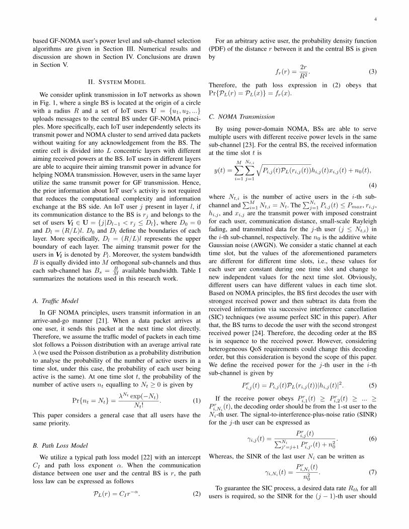
We consider uplink transmission in IoT networks as shownin Fig. 1, where a single BS is located at the origin of a circlewith a radius R and a set of IoT users U = {u1, u2, ...}uploads messages to the central BS under GF-NOMA princi-ples. More specifically, each IoT user independently selects itstransmit power and NOMA cluster to send arrived data packetswithout waiting for any acknowledgement from the BS. Theentire cell is divided into L concentric layers with differentaiming received powers at the BS. IoT users in different layersare able to acquire their aiming transmit power in advance forhelping NOMA transmission. However, users in the same layerutilize the same transmit power for GF transmission. Hence,the prior information about IoT user’s activity is not requiredthat reduces the computational complexity and informationexchange at the BS side. An IoT user j present in layer l, ifits communication distance to the BS is rj and belongs to theset of users Vl ∈ U = {j|Dl−1 < rj ≤ Dl}, where D0 = 0and Dl = (R/L)l. D0 and Dl define the boundaries of eachlayer. More specifically, Dl = (R/L)l represents the upperboundary of each layer. The aiming transmit power for theusers in Vl is denoted by Pl. Moreover, the system bandwidthB is equally divided into M orthogonal sub-channels and thuseach sub-channel has Bs = B

M available bandwidth. Table Isummarizes the notations used in this research work.

A. Traffic Model

In GF NOMA principles, users transmit information in anarrive-and-go manner [21]. When a data packet arrives atone user, it sends this packet at the next time slot directly.Therefore, we assume the traffic model of packets in each timeslot follows a Poisson distribution with an average arrival rateλ (we used the Poisson distribution as a probability distributionto analyse the probability of the number of active users in atime slot, under this case, the probability of each user beingactive is the same). At one time slot t, the probability of thenumber of active users nt equalling to Nt ≥ 0 is given by

Pr{nt = Nt} =λNt exp(−Nt)

Nt!. (1)

This paper considers a general case that all users have thesame priority.

B. Path Loss Model

We utilize a typical path loss model [22] with an interceptCI and path loss exponent α. When the communicationdistance between one user and the central BS is r, the pathloss law can be expressed as follows

PL(r) = CIr−α. (2)

For an arbitrary active user, the probability density function(PDF) of the distance r between it and the central BS is givenby

fr(r) =2r

R2. (3)

Therefore, the path loss expression in (2) obeys thatPr{PL(r) = PL(x)} = fr(x).

C. NOMA Transmission

By using power-domain NOMA, BSs are able to servemultiple users with different receive power levels in the samesub-channel [23]. For the central BS, the received informationat the time slot t is

y(t) =

M∑i=1

Nt,i∑j=1

√Pi,j(t)PL(ri,j(t))hi,j(t)xi,j(t) + n0(t),

(4)

where Nt,i is the number of active users in the i-th sub-channel and

∑Mi=1Nt,i = Nt. The

∑Ni

j=1 Pi,j(t) ≤ Pmax, ri,j ,hi,j , and xi,j are the transmit power with imposed constraintfor each user, communication distance, small-scale Rayleighfading, and transmitted data for the j-th user (j ≤ Nt,i) inthe i-th sub-channel, respectively. The n0 is the additive whiteGaussian noise (AWGN). We consider a static channel at eachtime slot, but the values of the aforementioned parametersare different for different time slots, i.e., these values foreach user are constant during one time slot and change tonew independent values for the next time slot. Obviously,different users can have different values in each time slot.Based on NOMA principles, the BS first decodes the user withstrongest received power and then subtract its data from thereceived information via successive interference cancellation(SIC) techniques (we assume perfect SIC in this paper). Afterthat, the BS turns to decode the user with the second strongestreceived power [24]. Therefore, the decoding order at the BSis in sequence to the received power. However, consideringheterogeneous QoS requirements could change this decodingorder, but this consideration is beyond the scope of this paper.We define the received power for the j-th user in the i-thsub-channel is given by

P ri,j(t) = Pi,j(t)PL(ri,j(t))|hi,j(t)|2. (5)

If the receive power obeys P ri,1(t) ≥ P ri,2(t) ≥ ... ≥P ri,Ni

(t), the decoding order should be from the 1-st user to theNi-th user. The signal-to-interference-plus-noise ratio (SINR)for the j-th user can be expressed as

γi,j(t) =P ri,j(t)∑Ni

j′=j+1 Pri,j′(t) + n20

. (6)

Whereas, the SINR of the last user Ni can be written as

γi,Ni(t) =P ri,Ni

(t)

n20. (7)

To guarantee the SIC process, a desired data rate Rth for allusers is required, so the SINR for the (j − 1)-th user should

5

TABLE I: Table of notations

Symbol Definition Symbol DefinitionU The set of entire IoT users Nt Number of active IoT users in a time slot tR Radius of the cell L Number of layers in cell areaVl Set of IoT users in layer l M Number of sub-channelsBs Sub-channel bandwidth Pl Transmit power level for set of IoT users in layer lri,j Communication distance between IoT user j and the BS n0 Additive white Gaussian noiseP ri,j(t) Received power of user j via sub-channel i γi,j(t) SINR of users j on sub-channel i

Ppool Prototype of transmit power pool Ep Number of transmit power levels in the designed power poolPBS Transmit power of BS Rth Date rate threshold requirement for successful SICki,j(t) Sub-channel selection variable for user j and sub-channel i Ri,j Data rate of user j on sub-channel iPt Matrix for transmit power levels Np Number of available transmit power levelsKt Matrix for sub-channel selection G Set of agents in MARL method

obeys Bs log2(1 + γi,j−1(t)) ≥ Rth, otherwise the BS cannotdecode information of the j-th user.

D. Layer-based Transmit Power Pool

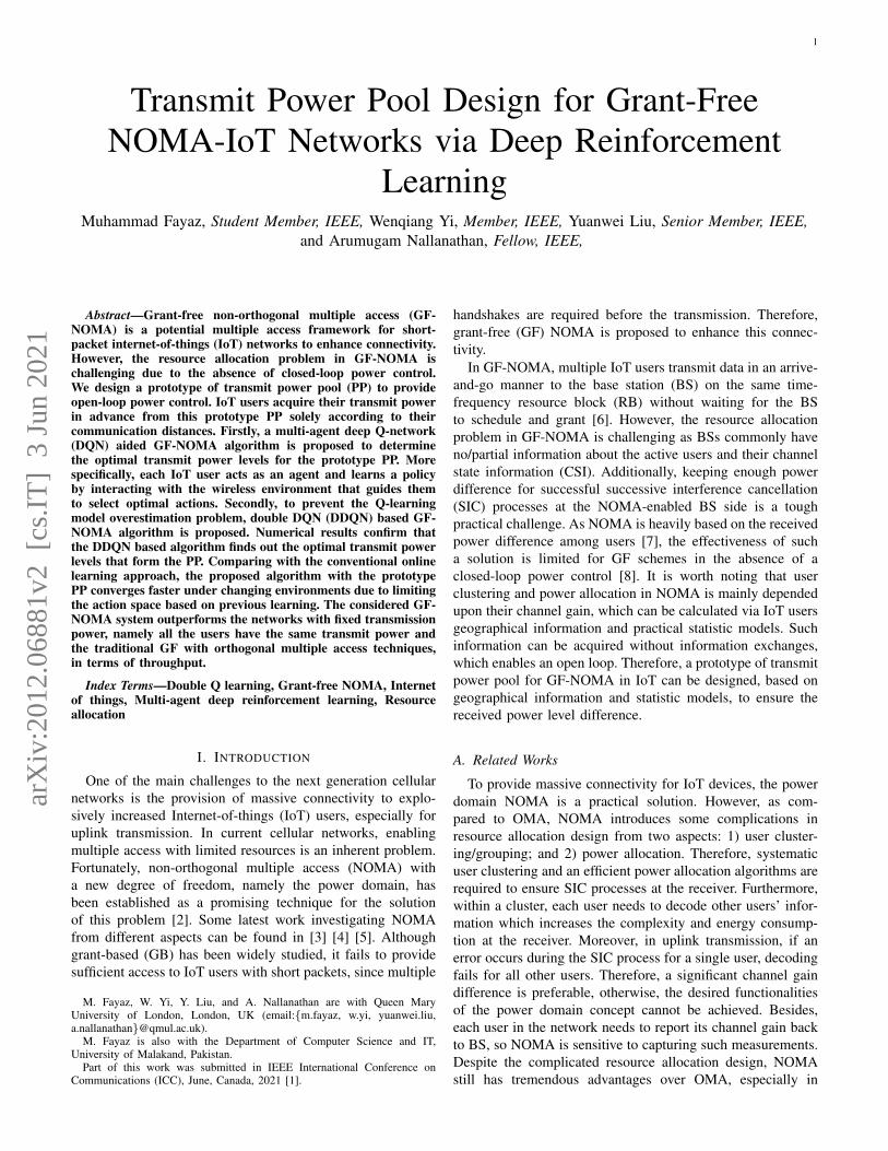
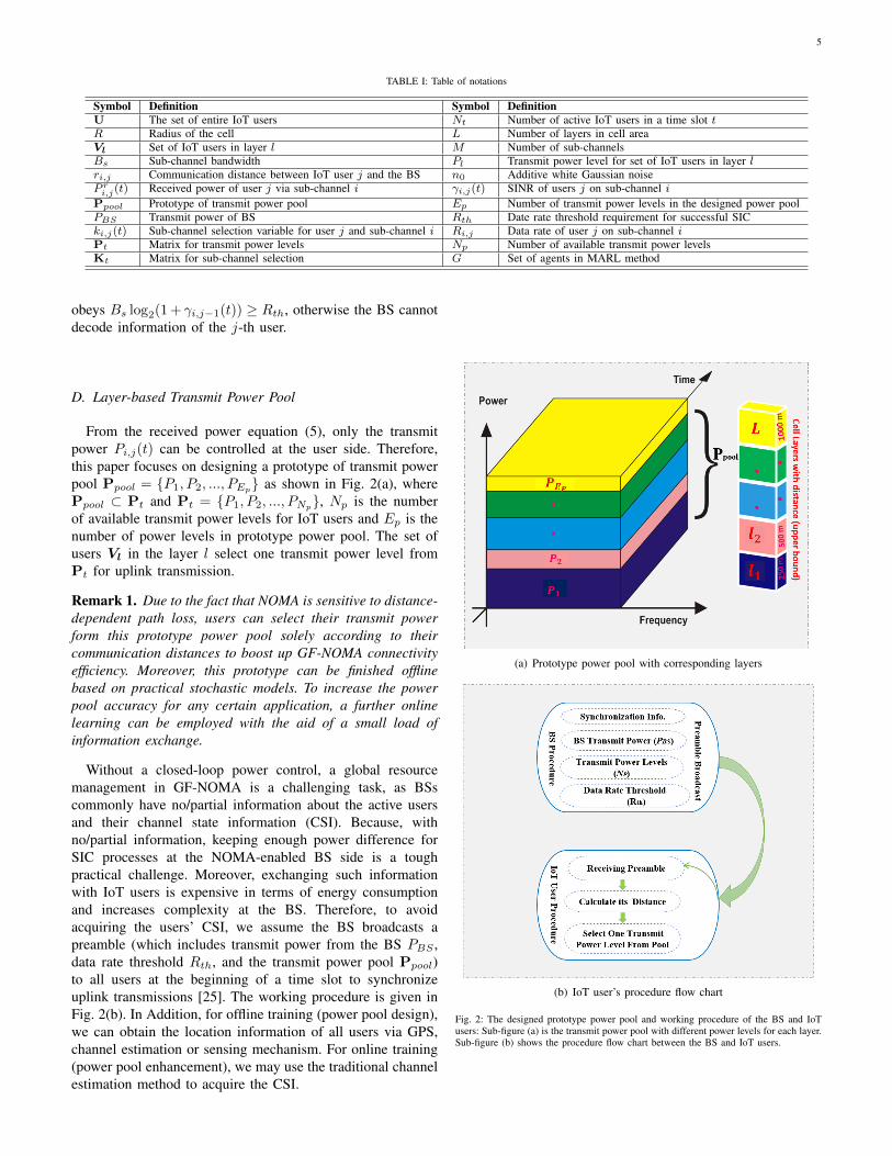
From the received power equation (5), only the transmitpower Pi,j(t) can be controlled at the user side. Therefore,this paper focuses on designing a prototype of transmit powerpool Ppool = {P1, P2, ..., PEp} as shown in Fig. 2(a), wherePpool ⊂ Pt and Pt = {P1, P2, ..., PNp

}, Np is the numberof available transmit power levels for IoT users and Ep is thenumber of power levels in prototype power pool. The set ofusers Vl in the layer l select one transmit power level fromPt for uplink transmission.

Remark 1. Due to the fact that NOMA is sensitive to distance-dependent path loss, users can select their transmit powerform this prototype power pool solely according to theircommunication distances to boost up GF-NOMA connectivityefficiency. Moreover, this prototype can be finished offlinebased on practical stochastic models. To increase the powerpool accuracy for any certain application, a further onlinelearning can be employed with the aid of a small load ofinformation exchange.

Without a closed-loop power control, a global resourcemanagement in GF-NOMA is a challenging task, as BSscommonly have no/partial information about the active usersand their channel state information (CSI). Because, withno/partial information, keeping enough power difference forSIC processes at the NOMA-enabled BS side is a toughpractical challenge. Moreover, exchanging such informationwith IoT users is expensive in terms of energy consumptionand increases complexity at the BS. Therefore, to avoidacquiring the users’ CSI, we assume the BS broadcasts apreamble (which includes transmit power from the BS PBS ,data rate threshold Rth, and the transmit power pool Ppool)to all users at the beginning of a time slot to synchronizeuplink transmissions [25]. The working procedure is given inFig. 2(b). In Addition, for offline training (power pool design),we can obtain the location information of all users via GPS,channel estimation or sensing mechanism. For online training(power pool enhancement), we may use the traditional channelestimation method to acquire the CSI.

(a) Prototype power pool with corresponding layers

(b) IoT user’s procedure flow chart

Fig. 2: The designed prototype power pool and working procedure of the BS and IoTusers: Sub-figure (a) is the transmit power pool with different power levels for each layer.Sub-figure (b) shows the procedure flow chart between the BS and IoT users.

6

E. Sub-Channel Selection

As NOMA provides the opportunity to multiplexed multipleusers on the same resource block (RB). Let Ni is the set ofusers sharing the i-th sub-channel. To form a NOMA cluster,the condition |Ni| > 1 must be satisfied. Furthermore, weassume that each IoT user is permitted to select at most onesub-channel. For a random IoT user j at time slot t, we definea sub-channel selection variable as follows:

ki,j(t) =

{1, IoT user j select sub-channel i

0, otherwise(8)

F. Problem Formulation

To determine the optimal transmit power levels for thedesign of prototype power pool, we formulate the sum ratemaximization as an optimization problem in this section.Therefore, maximizing the sum rate by optimizing the transmitpower and sub-channel selection for each user can contributeto the design of a transmit power pool that can be further allo-cated to a geographically distributed region. More specifically,two matrices Pt and Kt need to be optimized to maximizethe long-term sum rate. In each time slot t, the data rate of anIoT user j over sub-channel i can be written as

Ri,j(t) = Bs log2(1 + γi,j(t)) (9)

Therefore, the optimization problem can be formulated as

maxpi,j∈Pt,ki,j∈Kt

T∑t=1

M∑i=1

Ni∑j=1

Ri,j(t), (10)

s.t. P ri,1(t) ≥ P ri,2(t) ≥... ≥ P ri,Ni(t), ∀i,∀t, (10a)

Ni∑j=1

Pi,j(t) ≤ Pmax, ∀i,∀t, (10b)

M∑i=1

ki,j(t) ≤ 1, ∀j,∀t, (10c)

Ni(t) ≥ 2, ∀i,∀t, (10d)M∑i=1

Ri,j(t) ≥ Rmin(t), ∀j,∀t, (10e)

Ep < Np, (10f)Ep = L, (10g)

where (10a) is to ensure SIC decoding order, (10b) representsthe maximum power limit Pmax of each user, in (10c) thevariable ki,j indicates that at each time slot a user j is ableto select only one sub-channel, (10d) represents the minimumnumber of users on each sub-channel, (10e) guaranteeing theminimum required data rate Rmin of each IoT user, (10f)represents the number of power levels in the prototype powerpool Ppool (optimal power level for each layer), and (10g)represents power levels in the pool should be equal to thenumber of layers in cell area.

III. MULTI-AGENT DRL BASED POWER POOL DESIGN

A. Overview of Multi-Agent Deep Reinforcement Learning

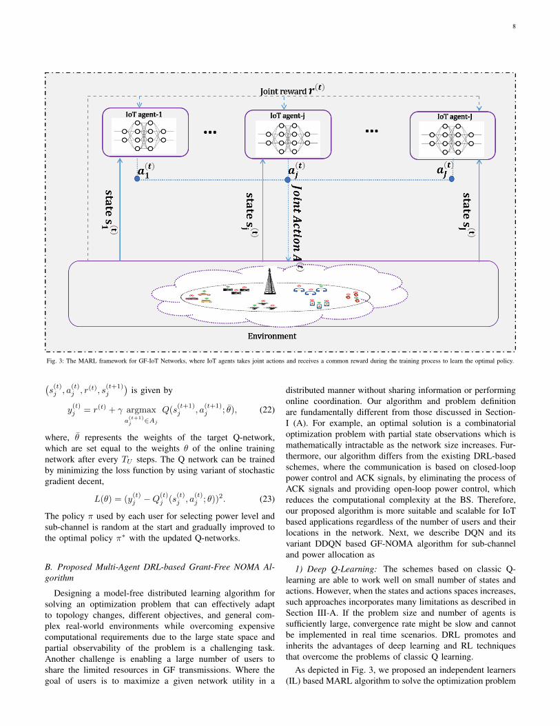
MARL is the extension of single agent RL which involvesa set of agents, G = {1, 2, 3 · · · · · · , N}, where the wholeteam of agents acting autonomously and concurrently in ashared environment. MARL can be classified into two cases:MARLs with centralized or decentralized reward. In MARLwith centralized rewards, all agents receive a common (central)reward, on the other hand in MARL with decentralized,every agent obtains a distinct reward [26]. However, in multi-agent environment, all agents under decentralized way maycompete with each other, i.e., agents may act in a selfishbehaviour for requiring the highest reward which may effectthe global network performance. To convert this selfishnessinto a cooperative behaviour, the same reward may be assignto all agents [27]. In next section, we apply MARL withcentralized reward only to prevent selfish behaviour of agents.

In MARL with centralized reward setting, a multi-agentMarkov decision process (MDP) can be represented by atuple of ({Sj}Nj=1, {Aj}Nj=1, P, r). Each agent j observes astate sj from the environment and executes an independentaction aj from its own set of actions Aj on the basis of itslocal policy πj : Sj → Aj . Agents perform joint action a(a = a1, a2, · · · , aN ∈ A), where A = (A1×A2×· · ·×AN ),the environment moves from state s

(t)j ∈ Sj to a new state

s(t+1)j ∈ Sj with probability of Pr(s(t)j |s

(t+1)j , aj), then the

agent j ∈ G receives a common reward r(t+1). Every agentforms an experience e(t+1)

j = (s(t)j , a

(t)j , r(t+1), s

(t+1)j ) at time

(t+1), which defines an interaction with the environment [28].The goal of each agent is to learn a local optimal policy π∗j thatforms a central optimal policy π∗ i.e. (π∗1 , π

∗2 , · · · , π∗N ) =: π∗

for maximizing long term reward [27].We model the selection of transmit power levels and sub-

channels in GF-NOMA IoT networks as MDP problem con-sisting of states s(t)j ∈ Sj , actions a(t)j ∈ Aj , and reward r(t)

following a policy πj . The main elements of the multi-agentDRL based GF-NOMA transmit power pool design are givenas follows:• State space S: To explore environment feature, each IoT

user j acts as an agent and simultaneously interacts withunknown environment. We define data rate of IoT usersas the current state s(t)j ∈ Sj , where

Sj = {R(t)1,1, R

(t)2,1,· · ·R

(t)i,j ,· · · , R

(t)M,N}, (11)

and Ri,j is the data rate of user j on sub-channel i in timeslot t. Moreover, the state size is equal to the number ofactive IoT users Nt in a time slot t.

• Action space A: Action a(t)j ∈ Aj of agent j ∈ G is

the selection of power level p ∈ P and sub-channel m ∈M . The transmission power is discretized into Np powerlevels, hence the dimension of action space is Np ×M ,where M is the number of sub-channels. The action spaceis given by

A = (A1 ×A2 × · · · ×Aj · · · ×AN ), (12)where Aj = {1, 2, · · ·pm, · · ·, PNp

M}. (13)

7

If an agent (IoT user) j transmits with power level pon sub-channel m in time slot t, then the correspondingaction is a(t)j ∈ Aj = pm, i.e., each action corresponds toa particular combination of power level and sub-channelselection.

• Reward Re: The system performance depends on re-ward function flexibility and its correlation with theobjective function [27]. To enhance system performancewe represent sum throughput of GF-NOMA system asa reward signal, which is strongly correlates with theobjective function. An agent j receives a returned rewardr(t) ∈ Re after choosing action a(t)j in state s(t)j in a TSt determined by

r(t) =

M∑i=1

Nt,i∑j=1

Ri,j . (14)

In our proposed model the short term reward of an agentj depends on the following conditions

r(t)j =

r(t), if Rcurrent ≥ Rprevious and

satisfying constraints given in

(10a)-(10e)

0, otherwise.

(15)

This reward or penalty can help agents to find optimalactions that can maximize cumulative reward for allinteractions with the environment.

Classic Q-Learning algorithm [29], aims to compute an opti-mal policy π∗ by maximizing expected reward. The long termdiscounted cumulative reward at time slot t is given by

Re(t) =

∞∑k=0

γkr(t+k+1), (16)

where γ ∈ [0, 1] is the discount factor. Q-Learning is based onaction-value function, the Q-function for IoT agent j which isdefined as the expected reward after taking action aj in statesj following a certain policy π [30], can be expressed as

Qπj (sj , aj) = Eπ[Re(t)

∣∣s(t)j = s, a(t)j = a

], (17)

where corresponding values of (17) is known as action valuesor Q-values and satisfies a Bellman equation,

Qπj (sj , aj) = R(sj , aj)+

γ∑s′j∈Sj

P asj→s′j

( ∑aj∈Aj

π(s′j , a′j)Q

π(s′j , a′j)), (18)

where R(sj , aj) is the immediate reward by taking action aj instate sj and P ajsj→s′j is the transition probability from state sj tonew state s′j by selecting action aj . By solving MDP each IoTagent is able to find the optimal policy π∗ to obtain maximalreward. The optimal Q-function for IoT agent j associated

with policy π∗ can be expressed as

Qπ∗

j (sj , aj) = R(sj , aj) + γ∑s′j∈Sj

Pajsj→s′j

maxa′j

Q∗(s′j , a′j).

(19)

The quality of a given action in a state can be measured by itscorresponding Q-value. To maximize its reward and improvepolicy π, agent j decides its action from

aj = argmaxaj∈Aj

Q(sj , aj). (20)

In Q-learning algorithm, to store Q-values of all possible state-action pairs, every agent needs to maintain a lookup table (Q-table), q(sj , aj) as a substitute of optimal Q-function. Afterrandom initialization of the Q-table, for each time step allthe agents take actions according to the ε-greedy policy. Withprobability ε, all agents decides actions randomly to avoidsticking in non-optimal policy, whereas with probability of1− ε, agents select actions that gives maximum Q-values forthe given state [28]. After taking action aj in a given state sj ,the agents acquire a new experience, and Q-learning algorithmupdates its corresponding Q-value in the Q-table.

During the decision process in a time slot t, if an agentj, given a state s(t)j , selecting action a(t)j , receiving a rewardr(t) and the next state s(t+1)

j , then its associated Q-value isupdated as

Q(s(t)j , a

(t)j )← r(t) + γ max

aj∈Aj

Q(s(t+1)j , aj). (21)

However, for IoT scenario, the size of Q-table increases withthe increasing number of state-action spaces (an increase ofIoT users) that makes Q-learning expensive in terms of mem-ory and computation because of the following two reasons..

1) Several states are infrequently visited, and2) Q-table storage in (21) becomes unrealistic.

In addition, DRL is one of the RL algorithms, which tendsto obtain more rewards as per its efficient learning behaviour,in comparison with the traditional Q-learning algorithm whichare prone to negative rewards [19].

To overcome the above problems, DRL (e.g. Deep QNetwork algorithm) is proposed, [28], in which the Q learningis combined with Deep Neural Network (DNN) for Q functionapproximation Q(s, a; θ), where θ represents its parameters(weights). Hence keeping a large storage space for state-actions pair (Q-values), DRL agent only memorize θ weightsin its local memory that reduces the memory and computationcomplexity.

In MARL based DRL setting, each agent j has a DQNthat takes the current state s(t)j as input and output Q-valuefunction of all actions. IoT agents explore the environmentby state-action pair following ε greedy policy. Every agentcollects and stores the experiences in the form of a tuple(s(t)j , a

(t)j , r(t), s

(t+1)j

)in replay memory. In each iteration, a

mini-batch of data is sampled uniformly from the memoryand is used to update network weights θ. The target valueproduced by target Q network from randomly sampled tuple

8

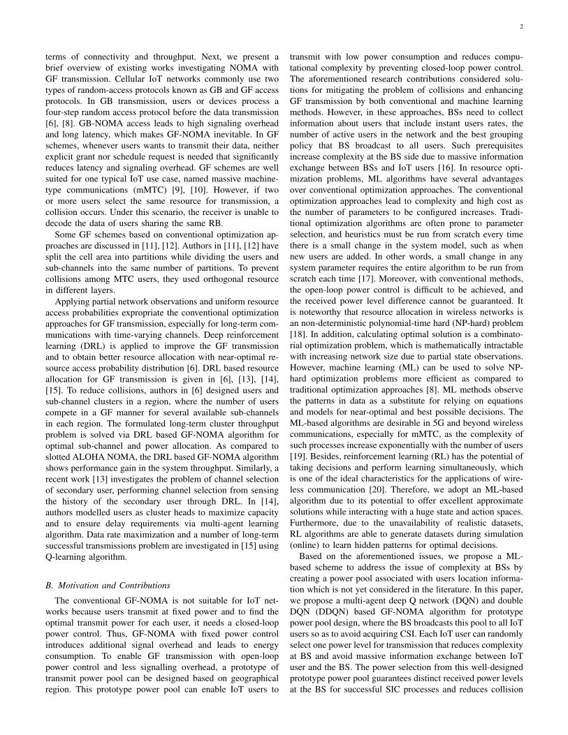
Fig. 3: The MARL framework for GF-IoT Networks, where IoT agents takes joint actions and receives a common reward during the training process to learn the optimal policy.

(s(t)j , a

(t)j , r(t), s

(t+1)j

)is given by

y(t)j = r(t) + γ argmax

a(t+1)j ∈Aj

Q(s(t+1)j , a

(t+1)j ; θ), (22)

where, θ represents the weights of the target Q-network,which are set equal to the weights θ of the online trainingnetwork after every TU steps. The Q network can be trainedby minimizing the loss function by using variant of stochasticgradient decent,

L(θ) = (y(t)j −Q

(t)j (s

(t)j , a

(t)j ; θ))2. (23)

The policy π used by each user for selecting power level andsub-channel is random at the start and gradually improved tothe optimal policy π∗ with the updated Q-networks.

B. Proposed Multi-Agent DRL-based Grant-Free NOMA Al-gorithm

Designing a model-free distributed learning algorithm forsolving an optimization problem that can effectively adaptto topology changes, different objectives, and general com-plex real-world environments while overcoming expensivecomputational requirements due to the large state space andpartial observability of the problem is a challenging task.Another challenge is enabling a large number of users toshare the limited resources in GF transmissions. Where thegoal of users is to maximize a given network utility in a

distributed manner without sharing information or performingonline coordination. Our algorithm and problem definitionare fundamentally different from those discussed in Section-I (A). For example, an optimal solution is a combinatorialoptimization problem with partial state observations which ismathematically intractable as the network size increases. Fur-thermore, our algorithm differs from the existing DRL-basedschemes, where the communication is based on closed-looppower control and ACK signals, by eliminating the process ofACK signals and providing open-loop power control, whichreduces the computational complexity at the BS. Therefore,our proposed algorithm is more suitable and scalable for IoTbased applications regardless of the number of users and theirlocations in the network. Next, we describe DQN and itsvariant DDQN based GF-NOMA algorithm for sub-channeland power allocation as

1) Deep Q-Learning: The schemes based on classic Q-learning are able to work well on small number of states andactions. However, when the states and actions spaces increases,such approaches incorporates many limitations as described inSection III-A. If the problem size and number of agents issufficiently large, convergence rate might be slow and cannotbe implemented in real time scenarios. DRL promotes andinherits the advantages of deep learning and RL techniquesthat overcome the problems of classic Q learning.

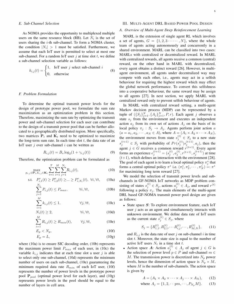
As depicted in Fig. 3, we proposed an independent learners(IL) based MARL algorithm to solve the optimization problem

9

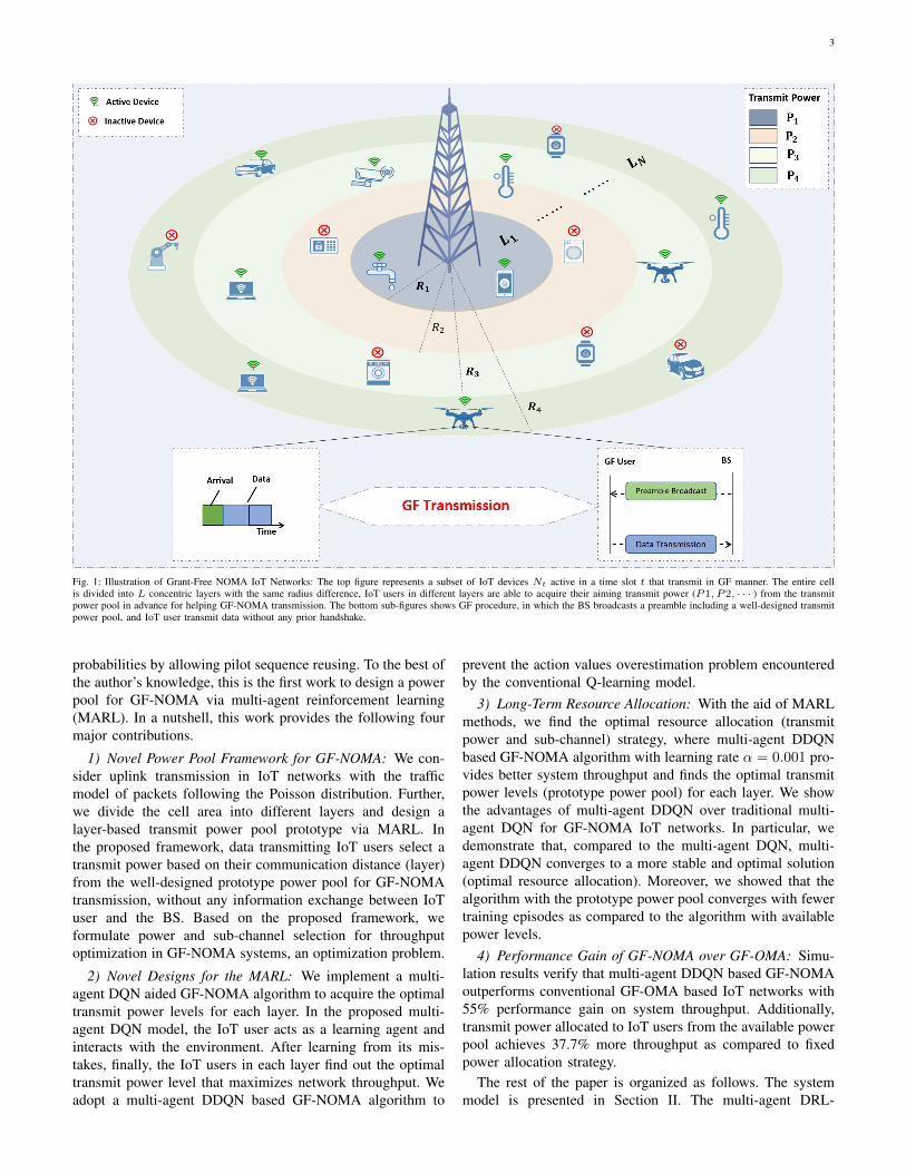
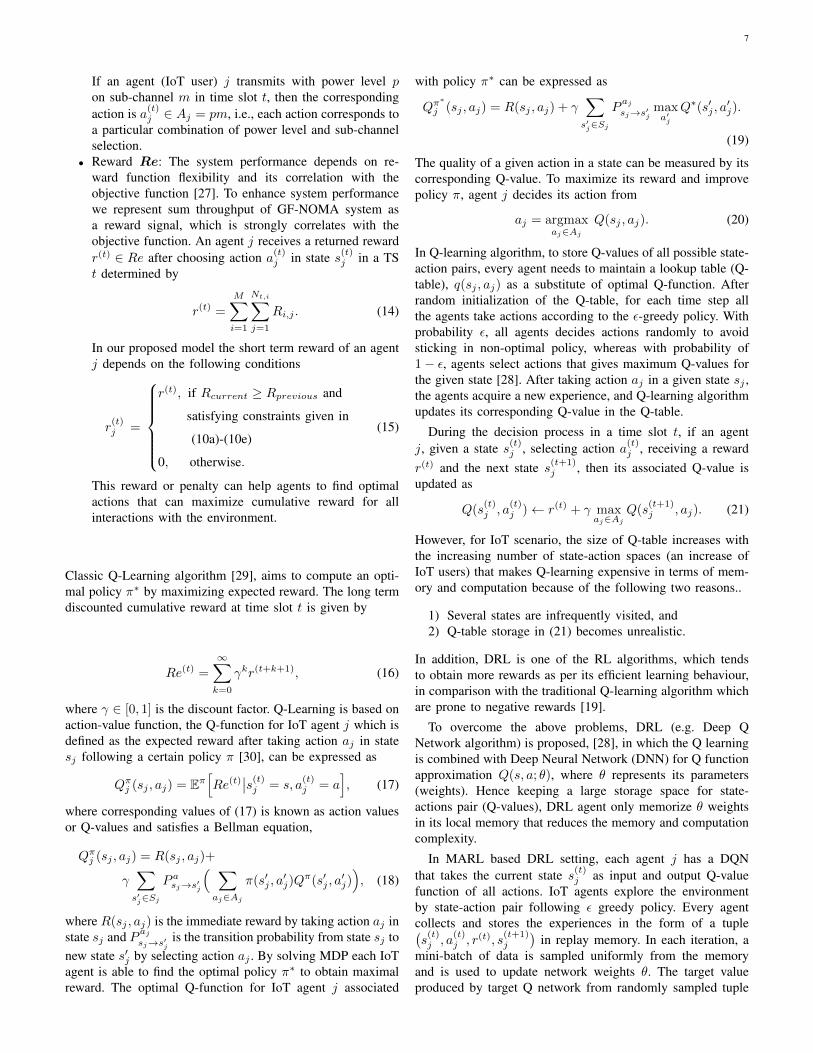
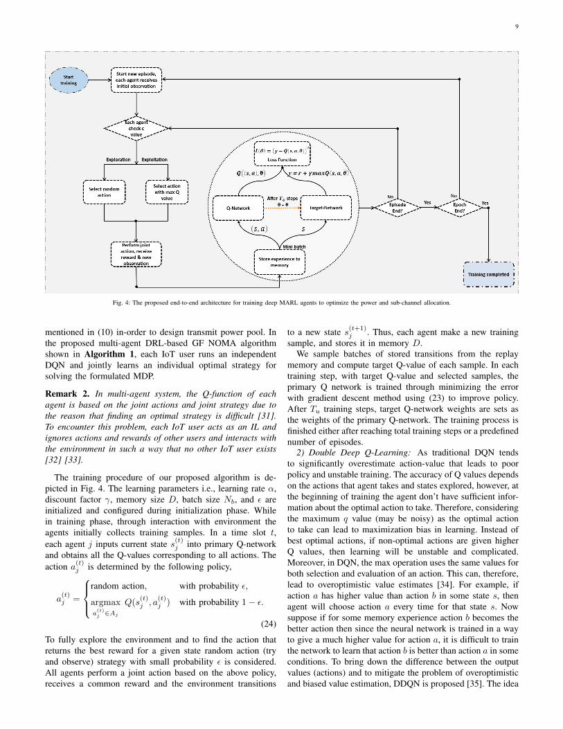
Fig. 4: The proposed end-to-end architecture for training deep MARL agents to optimize the power and sub-channel allocation.

mentioned in (10) in-order to design transmit power pool. Inthe proposed multi-agent DRL-based GF NOMA algorithmshown in Algorithm 1, each IoT user runs an independentDQN and jointly learns an individual optimal strategy forsolving the formulated MDP.

Remark 2. In multi-agent system, the Q-function of eachagent is based on the joint actions and joint strategy due tothe reason that finding an optimal strategy is difficult [31].To encounter this problem, each IoT user acts as an IL andignores actions and rewards of other users and interacts withthe environment in such a way that no other IoT user exists[32] [33].

The training procedure of our proposed algorithm is de-picted in Fig. 4. The learning parameters i.e., learning rate α,discount factor γ, memory size D, batch size Nb, and ε areinitialized and configured during initialization phase. Whilein training phase, through interaction with environment theagents initially collects training samples. In a time slot t,each agent j inputs current state s(t)j into primary Q-networkand obtains all the Q-values corresponding to all actions. Theaction a(t)j is determined by the following policy,

a(t)j =

random action, with probability ε,

argmaxa(t)j ∈Aj

Q(s(t)j , a

(t)j ) with probability 1− ε.

(24)

To fully explore the environment and to find the action thatreturns the best reward for a given state random action (tryand observe) strategy with small probability ε is considered.All agents perform a joint action based on the above policy,receives a common reward and the environment transitions

to a new state s(t+1)j . Thus, each agent make a new training

sample, and stores it in memory D.We sample batches of stored transitions from the replay

memory and compute target Q-value of each sample. In eachtraining step, with target Q-value and selected samples, theprimary Q network is trained through minimizing the errorwith gradient descent method using (23) to improve policy.After Tu training steps, target Q-network weights are sets asthe weights of the primary Q-network. The training process isfinished either after reaching total training steps or a predefinednumber of episodes.

2) Double Deep Q-Learning: As traditional DQN tendsto significantly overestimate action-value that leads to poorpolicy and unstable training. The accuracy of Q values dependson the actions that agent takes and states explored, however, atthe beginning of training the agent don’t have sufficient infor-mation about the optimal action to take. Therefore, consideringthe maximum q value (may be noisy) as the optimal actionto take can lead to maximization bias in learning. Instead ofbest optimal actions, if non-optimal actions are given higherQ values, then learning will be unstable and complicated.Moreover, in DQN, the max operation uses the same values forboth selection and evaluation of an action. This can, therefore,lead to overoptimistic value estimates [34]. For example, ifaction a has higher value than action b in some state s, thenagent will choose action a every time for that state s. Nowsuppose if for some memory experience action b becomes thebetter action then since the neural network is trained in a wayto give a much higher value for action a, it is difficult to trainthe network to learn that action b is better than action a in someconditions. To bring down the difference between the outputvalues (actions) and to mitigate the problem of overoptimisticand biased value estimation, DDQN is proposed [35]. The idea

10

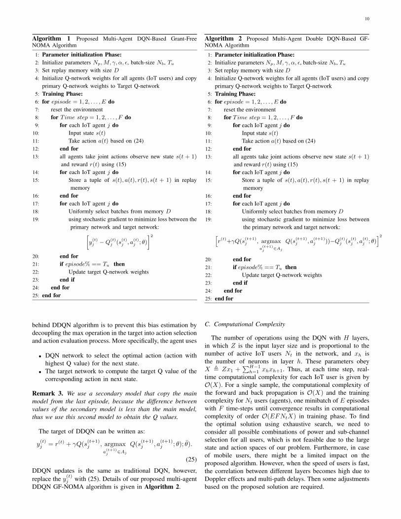
Algorithm 1 Proposed Multi-Agent DQN-Based Grant-FreeNOMA Algorithm

1: Parameter initialization Phase:2: Initialize parameters Np,M, γ, α, ε, batch-size Nb, Tu

3: Set replay memory with size D4: Initialize Q-network weights for all agents (IoT users) and copy

primary Q-network weights to Target Q-network5: Training Phase:6: for episode = 1, 2, . . . , E do7: reset the environment8: for T ime step = 1, 2, . . . , F do9: for each IoT agent j do

10: Input state s(t)11: Take action a(t) based on (24)12: end for13: all agents take joint actions observe new state s(t + 1)

and reward r(t) using (15)14: for each IoT agent j do15: Store a tuple of s(t), a(t), r(t), s(t + 1) in replay

memory16: end for17: for each IoT agent j do18: Uniformly select batches from memory D19: using stochastic gradient to minimize loss between the

primary network and target network:[y(t)j −Q

(t)j (s

(t)j , a

(t)j ; θ)

]220: end for21: if episode% == Tu then22: Update target Q-network weights23: end if24: end for25: end for

behind DDQN algorithm is to prevent this bias estimation bydecoupling the max operation in the target into action selectionand action evaluation process. More specifically, the agent uses

• DQN network to select the optimal action (action withhighest Q value) for the next state.

• The target network to compute the target Q value of thecorresponding action in next state.

Remark 3. We use a secondary model that copy the mainmodel from the last episode, because the difference betweenvalues of the secondary model is less than the main model,thus we use this second model to obtain the Q values.

The target of DDQN can be written as:

y(t)j = r(t) + γQ(s

(t+1)j , argmax

a(t+1)j ∈Aj

Q(s(t+1)j , a

(t+1)j ; θ); θ).

(25)

DDQN updates is the same as traditional DQN, however,replace the y(t)j with (25). Details of our proposed multi-agentDDQN GF-NOMA algorithm is given in Algorithm 2.

Algorithm 2 Proposed Multi-Agent Double DQN-Based GF-NOMA Algorithm

1: Parameter initialization Phase:2: Initialize parameters Np,M, γ, α, ε, batch-size Nb, Tu

3: Set replay memory with size D4: Initialize Q-network weights for all agents (IoT users) and copy

primary Q-network weights to Target Q-network5: Training Phase:6: for episode = 1, 2, . . . , E do7: reset the environment8: for T ime step = 1, 2, . . . , F do9: for each IoT agent j do

10: Input state s(t)11: Take action a(t) based on (24)12: end for13: all agents take joint actions observe new state s(t + 1)

and reward r(t) using (15)14: for each IoT agent j do15: Store a tuple of s(t), a(t), r(t), s(t + 1) in replay

memory16: end for17: for each IoT agent j do18: Uniformly select batches from memory D19: using stochastic gradient to minimize loss between

the primary network and target network:[r(t)+γQ(s

(t+1)j , argmax

a(t+1)j

∈Aj

Q(s(t+1)j , a

(t+1)j ))−Q(t)

j (s(t)j , a

(t)j ; θ)

]220: end for21: if episode% == Tu then22: Update target Q-network weights23: end if24: end for25: end for

C. Computational Complexity

The number of operations using the DQN with H layers,in which Z is the input layer size and is proportional to thenumber of active IoT users Nt in the network, and xh isthe number of neurons in layer h. These parameters obeyX , Zx1 +

∑H−1h=1 xhxh+1. Thus, at each time step, real-

time computational complexity for each IoT user is given byO(X). For a single sample, the computational complexity ofthe forward and back propagation is O(X) and the trainingcomplexity for Nt users (agents), one minibatch of E episodeswith F time-steps until convergence results in computationalcomplexity of order O(EFNtX) in training phase. To findthe optimal solution using exhaustive search, we need toconsider all possible combinations of power and sub-channelselection for all users, which is not feasible due to the largestate and action spaces of our problem. Furthermore, in caseof mobile users, there might be a limited impact on theproposed algorithm. However, when the speed of users is fast,the correlation between different layers becomes high due toDoppler effects and multi-path delays. Then some adjustmentsbased on the proposed solution are required.

11

IV. EXPERIMENTAL RESULTS

A. Simulation Setup and System Parameters

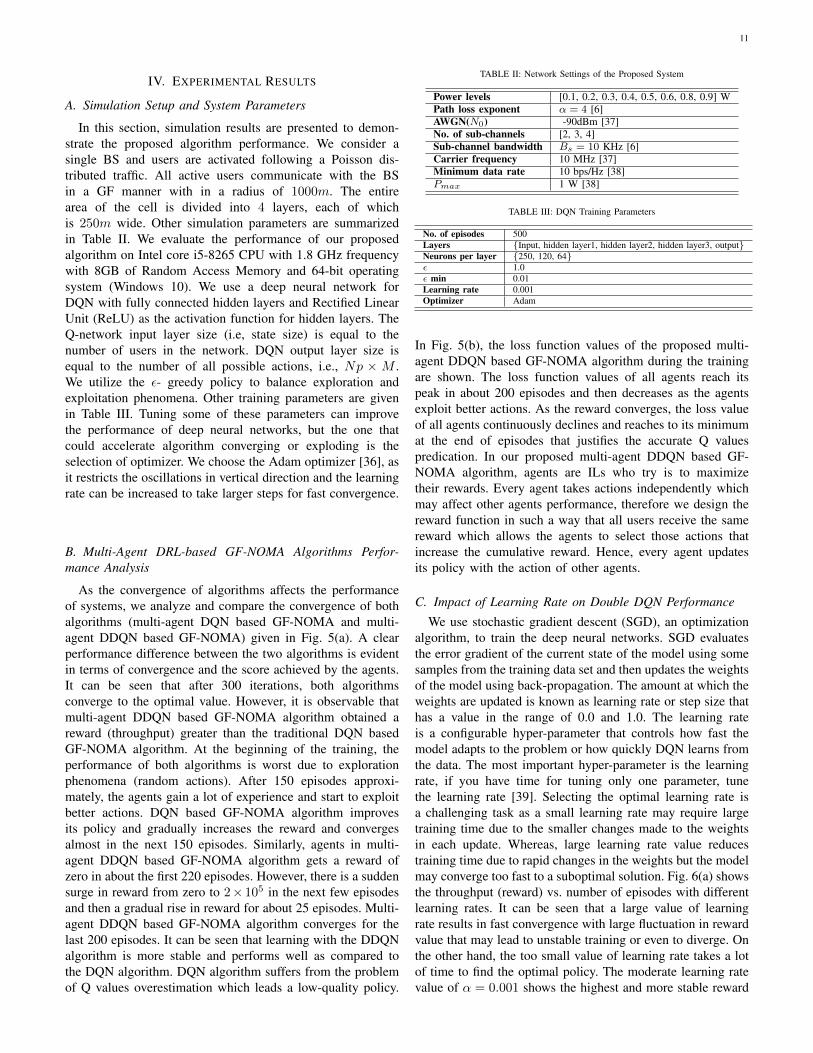
In this section, simulation results are presented to demon-strate the proposed algorithm performance. We consider asingle BS and users are activated following a Poisson dis-tributed traffic. All active users communicate with the BSin a GF manner with in a radius of 1000m. The entirearea of the cell is divided into 4 layers, each of whichis 250m wide. Other simulation parameters are summarizedin Table II. We evaluate the performance of our proposedalgorithm on Intel core i5-8265 CPU with 1.8 GHz frequencywith 8GB of Random Access Memory and 64-bit operatingsystem (Windows 10). We use a deep neural network forDQN with fully connected hidden layers and Rectified LinearUnit (ReLU) as the activation function for hidden layers. TheQ-network input layer size (i.e, state size) is equal to thenumber of users in the network. DQN output layer size isequal to the number of all possible actions, i.e., Np × M .We utilize the ε- greedy policy to balance exploration andexploitation phenomena. Other training parameters are givenin Table III. Tuning some of these parameters can improvethe performance of deep neural networks, but the one thatcould accelerate algorithm converging or exploding is theselection of optimizer. We choose the Adam optimizer [36], asit restricts the oscillations in vertical direction and the learningrate can be increased to take larger steps for fast convergence.

B. Multi-Agent DRL-based GF-NOMA Algorithms Perfor-mance Analysis

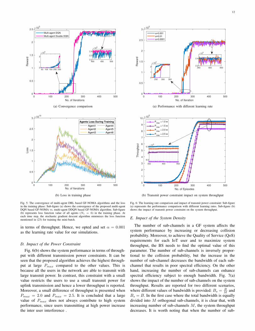
As the convergence of algorithms affects the performanceof systems, we analyze and compare the convergence of bothalgorithms (multi-agent DQN based GF-NOMA and multi-agent DDQN based GF-NOMA) given in Fig. 5(a). A clearperformance difference between the two algorithms is evidentin terms of convergence and the score achieved by the agents.It can be seen that after 300 iterations, both algorithmsconverge to the optimal value. However, it is observable thatmulti-agent DDQN based GF-NOMA algorithm obtained areward (throughput) greater than the traditional DQN basedGF-NOMA algorithm. At the beginning of the training, theperformance of both algorithms is worst due to explorationphenomena (random actions). After 150 episodes approxi-mately, the agents gain a lot of experience and start to exploitbetter actions. DQN based GF-NOMA algorithm improvesits policy and gradually increases the reward and convergesalmost in the next 150 episodes. Similarly, agents in multi-agent DDQN based GF-NOMA algorithm gets a reward ofzero in about the first 220 episodes. However, there is a suddensurge in reward from zero to 2× 105 in the next few episodesand then a gradual rise in reward for about 25 episodes. Multi-agent DDQN based GF-NOMA algorithm converges for thelast 200 episodes. It can be seen that learning with the DDQNalgorithm is more stable and performs well as compared tothe DQN algorithm. DQN algorithm suffers from the problemof Q values overestimation which leads a low-quality policy.

TABLE II: Network Settings of the Proposed System

Power levels [0.1, 0.2, 0.3, 0.4, 0.5, 0.6, 0.8, 0.9] WPath loss exponent α = 4 [6]AWGN(N0) -90dBm [37]No. of sub-channels [2, 3, 4]Sub-channel bandwidth Bs = 10 KHz [6]Carrier frequency 10 MHz [37]Minimum data rate 10 bps/Hz [38]Pmax 1 W [38]

TABLE III: DQN Training Parameters

No. of episodes 500Layers {Input, hidden layer1, hidden layer2, hidden layer3, output}Neurons per layer {250, 120, 64}ε 1.0ε min 0.01Learning rate 0.001Optimizer Adam

In Fig. 5(b), the loss function values of the proposed multi-agent DDQN based GF-NOMA algorithm during the trainingare shown. The loss function values of all agents reach itspeak in about 200 episodes and then decreases as the agentsexploit better actions. As the reward converges, the loss valueof all agents continuously declines and reaches to its minimumat the end of episodes that justifies the accurate Q valuespredication. In our proposed multi-agent DDQN based GF-NOMA algorithm, agents are ILs who try is to maximizetheir rewards. Every agent takes actions independently whichmay affect other agents performance, therefore we design thereward function in such a way that all users receive the samereward which allows the agents to select those actions thatincrease the cumulative reward. Hence, every agent updatesits policy with the action of other agents.

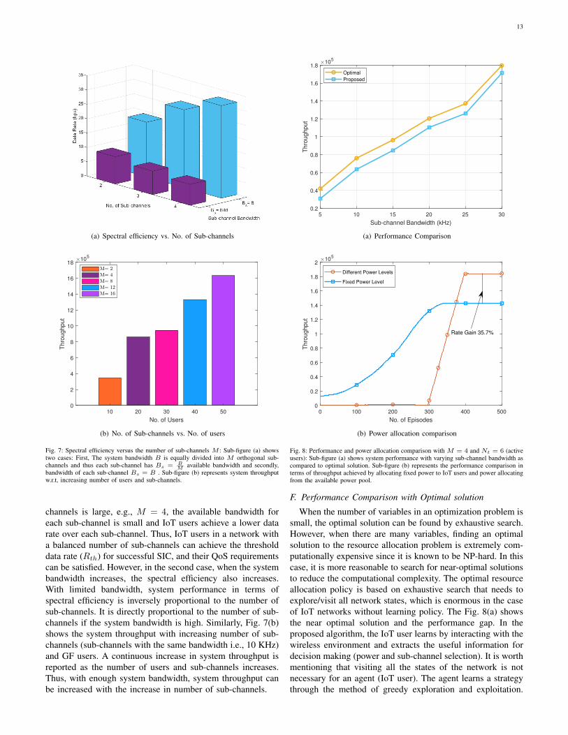
C. Impact of Learning Rate on Double DQN Performance

We use stochastic gradient descent (SGD), an optimizationalgorithm, to train the deep neural networks. SGD evaluatesthe error gradient of the current state of the model using somesamples from the training data set and then updates the weightsof the model using back-propagation. The amount at which theweights are updated is known as learning rate or step size thathas a value in the range of 0.0 and 1.0. The learning rateis a configurable hyper-parameter that controls how fast themodel adapts to the problem or how quickly DQN learns fromthe data. The most important hyper-parameter is the learningrate, if you have time for tuning only one parameter, tunethe learning rate [39]. Selecting the optimal learning rate isa challenging task as a small learning rate may require largetraining time due to the smaller changes made to the weightsin each update. Whereas, large learning rate value reducestraining time due to rapid changes in the weights but the modelmay converge too fast to a suboptimal solution. Fig. 6(a) showsthe throughput (reward) vs. number of episodes with differentlearning rates. It can be seen that a large value of learningrate results in fast convergence with large fluctuation in rewardvalue that may lead to unstable training or even to diverge. Onthe other hand, the too small value of learning rate takes a lotof time to find the optimal policy. The moderate learning ratevalue of α = 0.001 shows the highest and more stable reward

12

0 100 200 300 400 500

No. of Iterations

0

0.5

1

1.5

2

2.5R

ew

ard

105

Multi-agent DQN

Multi-agent Double DQN

50 100 150 200 2500

1

2

105

400 450 5002.2

2.3

2.4

105

(a) Convergence comparison

0 100 200 300 400 500

No. of Iterations

0

0.5

1

1.5

2

2.5

3

Loss

1010

Agent1

Agent2

Agent3

Agent4

Agent5

Agent6

Agents Loss During Training

(b) Loss in training phase

Fig. 5: The convergence of multi-agent DRL based GF-NOMA algorithms and the lossin the training phase: Sub-figure (a) shows the convergence of the proposed multi-agentDQN based GF-NOMA vs. multi-agent DDQN based GF-NOMA algorithm. Sub-figure(b) represents loss function value of all agents (Nt = 6) in the training phase. Ateach time step, the stochastic gradient descent algorithm minimizes the loss functionmentioned in (23) for training the mini-batch.

in terms of throughput. Hence, we opted and set α = 0.001as the learning rate value for our simulations.

D. Impact of the Power Constraint

Fig. 6(b) shows the system performance in terms of through-put with different transmission power constraints. It can beseen that the proposed algorithm achieves the highest through-put at large Pmax compared to the other values. This isbecause all the users in the network are able to transmit withlarge transmit power. In contrast, this constraint with a smallvalue restricts the users to use a small transmit power foruplink transmission and hence a lower throughput is reported.Moreover, a small difference of throughput is presented whenPmax = 2.0 and Pmax = 2.5. It is concluded that a largevalue of Pmax does not always contribute to high systemperformance, since users transmitting at high power increasethe inter user interference .

0 100 200 300 400 500

No. of Iteration

0

0.5

1

1.5

2

2.5

3

Rew

ard

105

250 300 3500

1

2

105

350 400 450

2.2

2.4

105

(a) Performance with different learning rate

0 100 200 300 400 500

No. of Episodes

0

1

2

3

4

5

6

7

8

9

10

Thro

ughput

105

Pmax

= 1.0 w

Pmax

= 1.5 w

Pmax

= 2.0 w

Pmax

= 2.5 w

350 400 450

8.5

9

9.510

5

(b) Transmit power constraint impact on system throughput

Fig. 6: The learning rate comparison and impact of transmit power constraint: Sub-figure(a) represents the performance comparison with different learning rates. Sub-figure (b)shows the impact of transmit power constraint on the system throughput.

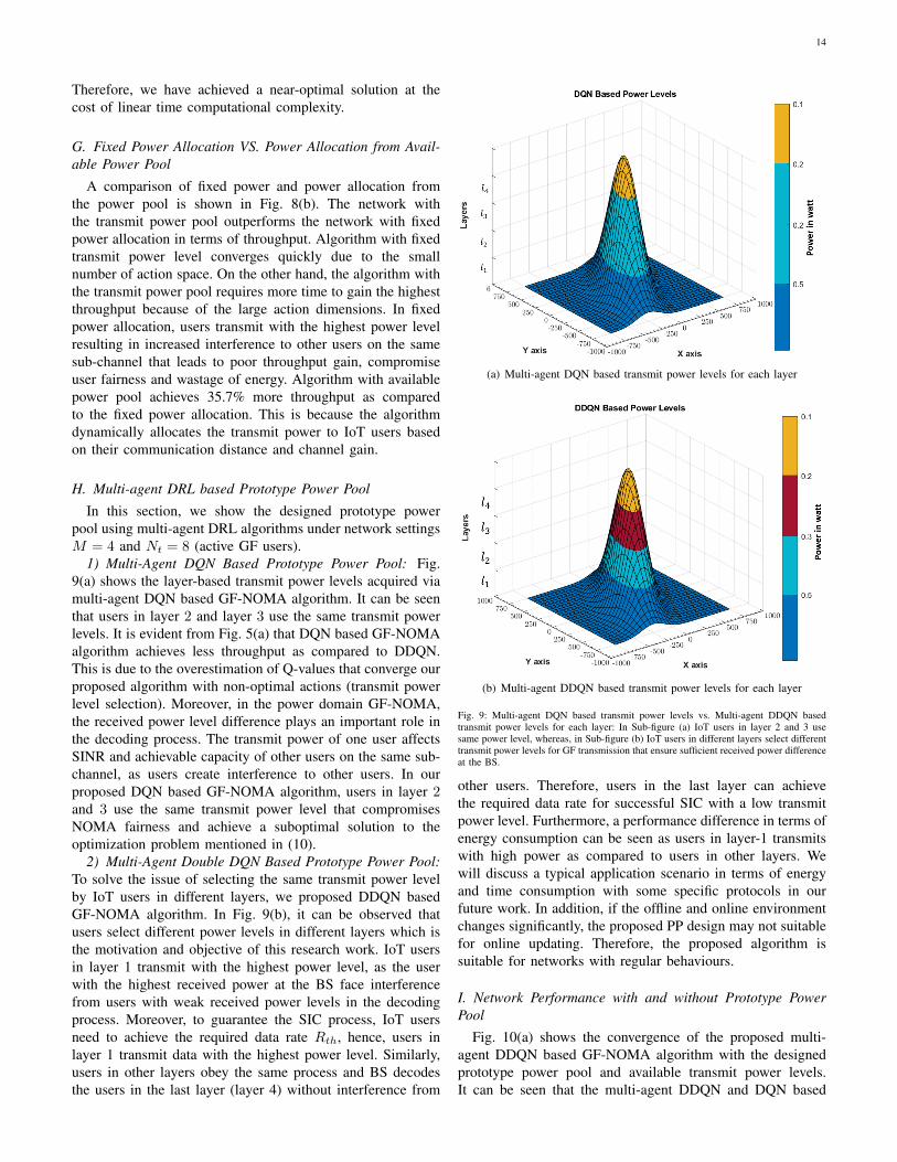
E. Impact of the System Density

The number of sub-channels in a GF system affects thesystem performance by increasing or decreasing collisionprobability. Moreover, to achieve the Quality of Service (QoS)requirements for each IoT user and to maximize systemthroughput, the BS needs to find the optimal value of thisparameter. The number of sub-channels is inversely propor-tional to the collision probability, but the increase in thenumber of sub-channel decreases the bandwidth of each sub-channel that results in poor spectral efficiency. On the otherhand, increasing the number of sub-channels can enhancespectral efficiency subject to enough bandwidth. Fig. 7(a)shows the impact of the number of sub-channels on the systemthroughput. Results are reported for two different scenarios,where different values of bandwidth is provided: Bs = B

M andBs = B. In the first case where the total bandwidth is equallydivided into M orthogonal sub-channels, it is clear that, withincreasing number of sub-channels M , the system throughputdecreases. It is worth noting that when the number of sub-

13

(a) Spectral efficiency vs. No. of Sub-channels

10 20 30 40 50

No. of Users

0

2

4

6

8

10

12

14

16

18

Thro

ughput

105

(b) No. of Sub-channels vs. No. of users

Fig. 7: Spectral efficiency versus the number of sub-channels M : Sub-figure (a) showstwo cases: First, The system bandwidth B is equally divided into M orthogonal sub-channels and thus each sub-channel has Bs = B

M available bandwidth and secondly,bandwidth of each sub-channel Bs = B . Sub-figure (b) represents system throughputw.r.t, increasing number of users and sub-channels.

channels is large, e.g., M = 4, the available bandwidth foreach sub-channel is small and IoT users achieve a lower datarate over each sub-channel. Thus, IoT users in a network witha balanced number of sub-channels can achieve the thresholddata rate (Rth) for successful SIC, and their QoS requirementscan be satisfied. However, in the second case, when the systembandwidth increases, the spectral efficiency also increases.With limited bandwidth, system performance in terms ofspectral efficiency is inversely proportional to the number ofsub-channels. It is directly proportional to the number of sub-channels if the system bandwidth is high. Similarly, Fig. 7(b)shows the system throughput with increasing number of sub-channels (sub-channels with the same bandwidth i.e., 10 KHz)and GF users. A continuous increase in system throughput isreported as the number of users and sub-channels increases.Thus, with enough system bandwidth, system throughput canbe increased with the increase in number of sub-channels.

5 10 15 20 25 30

Sub-channel Bandwidth (kHz)

0.2

0.4

0.6

0.8

1

1.2

1.4

1.6

1.8

Th

rou

gh

pu

t

105

Optimal

Proposed

(a) Performance Comparison

0 100 200 300 400 500

No. of Episodes

0

0.2

0.4

0.6

0.8

1

1.2

1.4

1.6

1.8

2

Thro

ughput

105

Different Power Levels

Fixed Power Level

Rate Gain 35.7%

(b) Power allocation comparison

Fig. 8: Performance and power allocation comparison with M = 4 and Nt = 6 (activeusers): Sub-figure (a) shows system performance with varying sub-channel bandwidth ascompared to optimal solution. Sub-figure (b) represents the performance comparison interms of throughput achieved by allocating fixed power to IoT users and power allocatingfrom the available power pool.

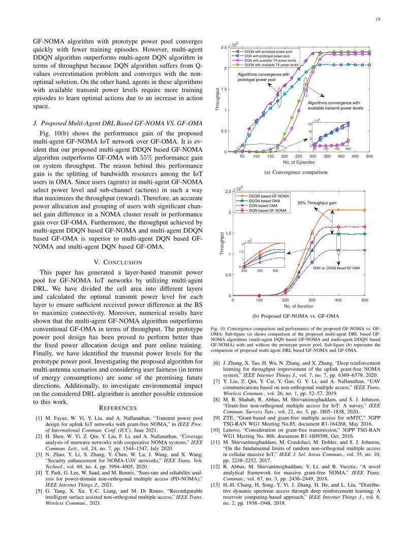
F. Performance Comparison with Optimal solution

When the number of variables in an optimization problem issmall, the optimal solution can be found by exhaustive search.However, when there are many variables, finding an optimalsolution to the resource allocation problem is extremely com-putationally expensive since it is known to be NP-hard. In thiscase, it is more reasonable to search for near-optimal solutionsto reduce the computational complexity. The optimal resourceallocation policy is based on exhaustive search that needs toexplore/visit all network states, which is enormous in the caseof IoT networks without learning policy. The Fig. 8(a) showsthe near optimal solution and the performance gap. In theproposed algorithm, the IoT user learns by interacting with thewireless environment and extracts the useful information fordecision making (power and sub-channel selection). It is worthmentioning that visiting all the states of the network is notnecessary for an agent (IoT user). The agent learns a strategythrough the method of greedy exploration and exploitation.

14

Therefore, we have achieved a near-optimal solution at thecost of linear time computational complexity.

G. Fixed Power Allocation VS. Power Allocation from Avail-able Power Pool

A comparison of fixed power and power allocation fromthe power pool is shown in Fig. 8(b). The network withthe transmit power pool outperforms the network with fixedpower allocation in terms of throughput. Algorithm with fixedtransmit power level converges quickly due to the smallnumber of action space. On the other hand, the algorithm withthe transmit power pool requires more time to gain the highestthroughput because of the large action dimensions. In fixedpower allocation, users transmit with the highest power levelresulting in increased interference to other users on the samesub-channel that leads to poor throughput gain, compromiseuser fairness and wastage of energy. Algorithm with availablepower pool achieves 35.7% more throughput as comparedto the fixed power allocation. This is because the algorithmdynamically allocates the transmit power to IoT users basedon their communication distance and channel gain.

H. Multi-agent DRL based Prototype Power Pool

In this section, we show the designed prototype powerpool using multi-agent DRL algorithms under network settingsM = 4 and Nt = 8 (active GF users).

1) Multi-Agent DQN Based Prototype Power Pool: Fig.9(a) shows the layer-based transmit power levels acquired viamulti-agent DQN based GF-NOMA algorithm. It can be seenthat users in layer 2 and layer 3 use the same transmit powerlevels. It is evident from Fig. 5(a) that DQN based GF-NOMAalgorithm achieves less throughput as compared to DDQN.This is due to the overestimation of Q-values that converge ourproposed algorithm with non-optimal actions (transmit powerlevel selection). Moreover, in the power domain GF-NOMA,the received power level difference plays an important role inthe decoding process. The transmit power of one user affectsSINR and achievable capacity of other users on the same sub-channel, as users create interference to other users. In ourproposed DQN based GF-NOMA algorithm, users in layer 2and 3 use the same transmit power level that compromisesNOMA fairness and achieve a suboptimal solution to theoptimization problem mentioned in (10).

2) Multi-Agent Double DQN Based Prototype Power Pool:To solve the issue of selecting the same transmit power levelby IoT users in different layers, we proposed DDQN basedGF-NOMA algorithm. In Fig. 9(b), it can be observed thatusers select different power levels in different layers which isthe motivation and objective of this research work. IoT usersin layer 1 transmit with the highest power level, as the userwith the highest received power at the BS face interferencefrom users with weak received power levels in the decodingprocess. Moreover, to guarantee the SIC process, IoT usersneed to achieve the required data rate Rth, hence, users inlayer 1 transmit data with the highest power level. Similarly,users in other layers obey the same process and BS decodesthe users in the last layer (layer 4) without interference from

(a) Multi-agent DQN based transmit power levels for each layer

(b) Multi-agent DDQN based transmit power levels for each layer

Fig. 9: Multi-agent DQN based transmit power levels vs. Multi-agent DDQN basedtransmit power levels for each layer: In Sub-figure (a) IoT users in layer 2 and 3 usesame power level, whereas, in Sub-figure (b) IoT users in different layers select differenttransmit power levels for GF transmission that ensure sufficient received power differenceat the BS.

other users. Therefore, users in the last layer can achievethe required data rate for successful SIC with a low transmitpower level. Furthermore, a performance difference in terms ofenergy consumption can be seen as users in layer-1 transmitswith high power as compared to users in other layers. Wewill discuss a typical application scenario in terms of energyand time consumption with some specific protocols in ourfuture work. In addition, if the offline and online environmentchanges significantly, the proposed PP design may not suitablefor online updating. Therefore, the proposed algorithm issuitable for networks with regular behaviours.

I. Network Performance with and without Prototype PowerPool

Fig. 10(a) shows the convergence of the proposed multi-agent DDQN based GF-NOMA algorithm with the designedprototype power pool and available transmit power levels.It can be seen that the multi-agent DDQN and DQN based

15

GF-NOMA algorithm with prototype power pool convergesquickly with fewer training episodes. However, multi-agentDDQN algorithm outperforms multi-agent DQN algorithm interms of throughput because DQN algorithm suffers from Q-values overestimation problem and converges with the non-optimal solution. On the other hand, agents in these algorithmswith available transmit power levels require more trainingepisodes to learn optimal actions due to an increase in actionspace.

J. Proposed Multi-Agent DRL Based GF-NOMA VS. GF-OMA

Fig. 10(b) shows the performance gain of the proposedmulti-agent GF-NOMA IoT network over GF-OMA. It is ev-ident that our proposed multi-agent DDQN based GF-NOMAalgorithm outperforms GF-OMA with 55% performance gainon system throughput. The reason behind this performancegain is the splitting of bandwidth resources among the IoTusers in OMA. Since users (agents) in multi-agent GF-NOMAselect power level and sub-channel (actions) in such a waythat maximizes the throughput (reward). Therefore, an accuratepower allocation and grouping of users with significant chan-nel gain difference in a NOMA cluster result in performancegain over GF-OMA. Furthermore, the throughput achieved bymulti-agent DDQN based GF-NOMA and multi-agent DDQNbased GF-OMA is superior to multi-agent DQN based GF-NOMA and multi-agent DQN based GF-OMA.

V. CONCLUSION

This paper has generated a layer-based transmit powerpool for GF-NOMA IoT networks by utilizing multi-agentDRL. We have divided the cell area into different layersand calculated the optimal transmit power level for eachlayer to ensure sufficient received power difference at the BSto maximize connectivity. Moreover, numerical results haveshown that the multi-agent GF-NOMA algorithm outperformsconventional GF-OMA in terms of throughput. The prototypepower pool design has been proved to perform better thanthe fixed power allocation design and pure online training.Finally, we have identified the transmit power levels for theprototype power pool. Investigating the proposed algorithm formulti-antenna scenarios and considering user fairness (in termsof energy consumptions) are some of the promising futuredirections. Additionally, to investigate environmental impacton the considered DRL algorithm is another possible extensionto this work.

REFERENCES

[1] M. Fayaz, W. Yi, Y. Liu, and A. Nallanathan, “Transmit power pooldesign for uplink IoT networks with grant-free NOMA,” in IEEE Proc.of International Commun. Conf. (ICC), June 2021.

[2] H. Shen, W. Yi, Z. Qin, Y. Liu, F. Li, and A. Nallanathan, “Coverageanalysis of mmwave networks with cooperative NOMA systems,” IEEECommun. Lett., vol. 24, no. 7, pp. 1544–1547, July 2020.

[3] N. Zhao, Y. Li, S. Zhang, Y. Chen, W. Lu, J. Wang, and X. Wang,“Security enhancement for NOMA-UAV networks,” IEEE Trans. Veh.Technol., vol. 69, no. 4, pp. 3994–4005, 2020.

[4] T. Park, G. Lee, W. Saad, and M. Bennis, “Sum-rate and reliability anal-ysis for power-domain non-orthogonal multiple access (PD-NOMA),”IEEE Internet Things J., 2021.

[5] G. Yang, X. Xu, Y.-C. Liang, and M. Di Renzo, “Reconfigurableintelligent surface assisted non-orthogonal multiple access,” IEEE Trans.Wireless Commun., 2021.

50 100 150 200 250 300 350 400 450 500

No. of Episodes

0

0.5

1

1.5

2

2.5

Thro

ughput

105

DDQN with prototype power pool

DQN with prototype power pool

DQN with available TX power levels

DDQN with available TX power levels

50 100 150 2000

5

10

1510

4

Algorithms convergence with

prototype power pool

Algorithms convergence with

available transmit power levels

(a) Convergence comparison

0 100 200 300 400 500

No. of Iteration

0

0.5

1

1.5

2

2.5

Thro

ughput

105

DDQN based GF-NOMA

DDQN based OMA

DQN based OMA

DQN based GF-NOMA

250 300 3500.5

1

1.5

210

5

DQN vs. DDQN Based GF-OMA

55% Throughput gain

(b) Proposed GF-NOMA vs. GF-OMA

Fig. 10: Convergence comparison and performance of the proposed GF-NOMA vs. GF-OMA: Sub-figure (a) shows comparison of the proposed multi-agent DRL based GF-NOMA algorithms (multi-agent DQN based GF-NOMA and multi-agent DDQN basedGF-NOMA) with and without the prototype power pool. Sub-figure (b) represents thecomparison of proposed multi-agent DRL based GF-NOMA and GF-OMA.

[6] J. Zhang, X. Tao, H. Wu, N. Zhang, and X. Zhang, “Deep reinforcementlearning for throughput improvement of the uplink grant-free NOMAsystem,” IEEE Internet Things J., vol. 7, no. 7, pp. 6369–6379, 2020.

[7] Y. Liu, Z. Qin, Y. Cai, Y. Gao, G. Y. Li, and A. Nallanathan, “UAVcommunications based on non-orthogonal multiple access,” IEEE Trans.Wireless Commun., vol. 26, no. 1, pp. 52–57, 2019.

[8] M. B. Shahab, R. Abbas, M. Shirvanimoghaddam, and S. J. Johnson,“Grant-free non-orthogonal multiple access for IoT: A survey,” IEEECommun. Surveys Tuts., vol. 22, no. 3, pp. 1805–1838, 2020.

[9] ZTE, “Grant-based and grant-free multiple access for mMTC,” 3GPPTSG-RAN WG1 Meeting No.85, document R1-164268, May 2016.

[10] Lenovo, “Consideration on grant-free transmission,” 3GPP TSG-RANWG1 Meeting No. 86b, document R1-1609398, Oct. 2016.

[11] M. Shirvanimoghaddam, M. Condoluci, M. Dohler, and S. J. Johnson,“On the fundamental limits of random non-orthogonal multiple accessin cellular massive IoT,” IEEE J. Sel. Areas Commun., vol. 35, no. 10,pp. 2238–2252, 2017.

[12] R. Abbas, M. Shirvanimoghaddam, Y. Li, and B. Vucetic, “A novelanalytical framework for massive grant-free NOMA,” IEEE Trans.Commun., vol. 67, no. 3, pp. 2436–2449, 2018.

[13] H.-H. Chang, H. Song, Y. Yi, J. Zhang, H. He, and L. Liu, “Distribu-tive dynamic spectrum access through deep reinforcement learning: Areservoir computing-based approach,” IEEE Internet Things J., vol. 6,no. 2, pp. 1938–1948, 2018.

16

[14] Y. Xu, J. Wang, Q. Wu, J. Zheng, L. Shen, and A. Anpalagan, “Dynamicspectrum access in time-varying environment: Distributed learning be-yond expectation optimization,” IEEE Trans. Commun., vol. 65, no. 12,pp. 5305–5318, 2017.

[15] S. Wang, H. Liu, P. H. Gomes, and B. Krishnamachari, “Deep reinforce-ment learning for dynamic multichannel access in wireless networks,”IEEE Trans. Cogn. Commun. Netw., vol. 4, no. 2, pp. 257–265, 2018.

[16] X. Chen, D. W. K. Ng, W. Yu, E. G. Larsson, N. Al-Dhahir, andR. Schober, “Massive access for 5G and beyond,” IEEE J. Sel. AreasCommun., pp. 1–1, 2020.

[17] O. Maraqa, A. S. Rajasekaran, S. Al-Ahmadi, H. Yanikomeroglu, andS. M. Sait, “A survey of rate-optimal power domain NOMA withenabling technologies of future wireless networks,” IEEE Commun.Surveys Tuts., vol. 22, no. 4, pp. 2192–2235, 2020.

[18] J. Zuo, Y. Liu, Z. Qin, and N. Al-Dhahir, “Resource allocation inintelligent reflecting surface assisted NOMA systems,” IEEE Trans.Commun., vol. 68, no. 11, pp. 7170–7183, 2020.

[19] W. Ahsan, W. Yi, Z. Qin, Y. Liu, and A. Nallanathan, “Resourceallocation in uplink NOMA-IoT networks: A reinforcement-learningapproach,” arXiv preprint arXiv:2007.08350, 2020.

[20] N. C. Luong, D. T. Hoang, S. Gong, D. Niyato, P. Wang, Y.-C.Liang, and D. I. Kim, “Applications of deep reinforcement learning incommunications and networking: A survey,” IEEE Commun. SurveysTuts., vol. 21, no. 4, pp. 3133–3174, 2019.

[21] J. Zhang, L. Lu, Y. Sun, Y. Chen, J. Liang, J. Liu, H. Yang, S. Xing,Y. Wu, J. Ma et al., “PoC of SCMA-based uplink grant-free transmissionin UCNC for 5G,” IEEE J. Sel. Areas Commun., vol. 35, no. 6, pp.1353–1362, 2017.

[22] W. Yi, Y. Liu, E. Bodanese, A. Nallanathan, and G. K. Karagiannidis,“A unified spatial framework for UAV-aided mmwave networks,” IEEETrans. Commun., vol. 67, no. 12, pp. 8801–8817, Dec. 2019.

[23] X. Mu, Y. Liu, L. Guo, J. Lin, and N. Al-Dhahir, “Exploiting intelligentreflecting surfaces in NOMA networks: Joint beamforming optimiza-tion,” IEEE Trans. Wireless Commun., vol. 19, no. 10, pp. 6884–6898,2020.

[24] Y. Liu, Z. Qin, M. Elkashlan, Z. Ding, A. Nallanathan, and L. Hanzo,“Nonorthogonal multiple access for 5G and beyond,” Proceedings of theIEEE, vol. 105, no. 12, pp. 2347–2381, Dec. 2017.

[25] J. Choi, “NOMA-based random access with multichannel aloha,” IEEEJ. Sel. Areas Commun., vol. 35, no. 12, pp. 2736–2743, Dec 2017.

[26] D. Lee, N. He, P. Kamalaruban, and V. Cevher, “Optimization forreinforcement learning: From a single agent to cooperative agents,” IEEESignal Process. Mag., vol. 37, no. 3, pp. 123–135, 2020.

[27] L. Liang, H. Ye, and G. Y. Li, “Spectrum sharing in vehicular networksbased on multi-agent reinforcement learning,” IEEE J. Sel. Areas Com-mun., vol. 37, no. 10, pp. 2282–2292, 2019.

[28] V. Mnih, K. Kavukcuoglu, D. Silver, A. A. Rusu, J. Veness, M. G.Bellemare, A. Graves, M. Riedmiller, A. K. Fidjeland, G. Ostrovskiet al., “Human-level control through deep reinforcement learning,”Nature, vol. 518, no. 7540, pp. 529–533, 2015.

[29] R. S. Sutton and A. G. Barto, Reinforcement learning: An introduction.MIT press, 2018.

[30] S. Singh, T. Jaakkola, M. L. Littman, and C. Szepesvari, “Convergenceresults for single-step on-policy reinforcement-learning algorithms,”Machine learning, vol. 38, no. 3, pp. 287–308, 2000.

[31] G. Neto, “From single-agent to multi-agent reinforcement learning:Foundational concepts and methods,” Learning theory course, 2005.

[32] J. Cui, Y. Liu, and A. Nallanathan, “Multi-agent reinforcement learning-based resource allocation for UAV networks,” IEEE Trans. WirelessCommun., vol. 19, no. 2, pp. 729–743, 2019.

[33] X. Liu, J. Yu, Z. Feng, and Y. Gao, “Multi-agent reinforcement learningfor resource allocation in iot networks with edge computing,” ChinaCommunications, vol. 17, no. 9, pp. 220–236, 2020.

[34] K. K. Nguyen, T. Q. Duong, N. A. Vien, N.-A. Le-Khac, and M.-N. Nguyen, “Non-cooperative energy efficient power allocation gamein D2D communication: A multi-agent deep reinforcement learningapproach,” IEEE Access, vol. 7, pp. 100 480–100 490, 2019.

[35] H. Van Hasselt, A. Guez, and D. Silver, “Deep reinforcement learningwith double q-learning,” arXiv preprint arXiv:1509.06461, 2015.

[36] D. P. Kingma and J. Ba, “Adam: A method for stochastic optimization,”arXiv preprint arXiv:1412.6980, 2014.

[37] C. Zhang, Y. Liu, Z. Qin, and Z. Ding, “Semi-grant-free NOMA: Astochastic geometry model,” arXiv preprint arXiv:2006.13286, 2020.

[38] X. Wang, Y. Zhang, R. Shen, Y. Xu, and F. C. Zheng, “DRL-basedenergy-efficient resource allocation frameworks for uplink NOMA sys-tems,” IEEE Internet Things J., vol. 7, no. 8, pp. 7279–7294, 2020.

[39] I. Goodfellow, Y. Bengio, A. Courville, and Y. Bengio, Deep learning.MIT press Cambridge, 2016, vol. 1.