Embed Size (px)
Citation preview
TRANSFORMER MODELLING AND INFLUENTIAL
PARAMETERS IDENTIFICATION FOR GEOMAGNETIC
DISTURBANCES EVENTS
A thesis submitted to The University of Manchester for the degree of
PhD
In the Faculty of Engineering and Physical Sciences
2012
RUI ZHANG
School of Electrical and Electronic Engineering


Contents
3
CONTENTS CONTENTS ............................................................................................................................................. 3
LIST OF FIGURES .................................................................................................................................... 6
LIST OF TABLES .....................................................................................................................................12
LIST OF SYMBOL ...................................................................................................................................14
ABSTRACT ............................................................................................................................................17
DECLARATION ......................................................................................................................................18
COPYRIGHT STATEMENT ......................................................................................................................19
ACKNOWLEDGEMENT ..........................................................................................................................20
CHAPTER 1 INTRODUCTION .............................................................................................................21
1.1 INTRODUCTION .................................................................................................................................... 21
1.2 TRANSFORMER CORE SATURATION PROBLEMS ............................................................................................ 21
1.2.1 Inrush currents ......................................................................................................................... 22
1.2.2 Ferroresonance ........................................................................................................................ 24
1.2.3 Geomagnetic induced currents (GIC) ....................................................................................... 26
1.3 OBJECTIVES ......................................................................................................................................... 29
1.4 MAJOR CONTRIBUTION AND ORIGINALITY .................................................................................................. 31
1.5 THESIS OUTLINE .................................................................................................................................... 32
CHAPTER 2 BASICS OF TRANSFORMERS ...........................................................................................34
2.1 INTRODUCTION .................................................................................................................................... 34
2.2 TRANSFORMER STRUCTURE ..................................................................................................................... 34
2.2.1 Main component---winding ..................................................................................................... 35
2.2.2 Main component---transformer core ....................................................................................... 36
2.2.3 Transformer core materials ..................................................................................................... 39
CHAPTER 3 LITERATURE REVIEW .....................................................................................................45
3.1 INTRODUCTION .................................................................................................................................... 45
3.2 POWER SYSTEM OPERATION TRANSIENT---SWITCHING TRANSIENTS ................................................................. 46
3.2.1 Background .............................................................................................................................. 46
3.2.2 Ferroresonance ........................................................................................................................ 47
3.3 POWER SYSTEM NATURAL TRANSIENT---GIC .............................................................................................. 60
3.3.1 Background .............................................................................................................................. 60
3.3.2 GIC effect on power system ..................................................................................................... 61
3.3.3 Historical events....................................................................................................................... 64

Contents
4
3.3.4 Studies on transformer responses to GIC .................................................................................67
3.3.5 Mitigation .................................................................................................................................77
3.4 DISCUSSION AND SUMMARY ....................................................................................................................80
CHAPTER 4 STEADY STATE MAGNETIC CIRCUIT MODELLING FOR TRANSFORMERS ......................... 82
4.1 METHODOLOGY OF TRANSFORMER CORE MODELLING ...................................................................................83
4.1.1 Three-limb transformer core model .........................................................................................83
4.1.2 Five-limb transformer core model ............................................................................................87
4.1.3 Magnetising current calculation ..............................................................................................89
4.1.4 Flux density calculation ............................................................................................................90
4.1.5 Curve fitting ..............................................................................................................................93
4.2 CASE 1: MAGNETISING CURRENT INVESTIGATION ........................................................................................94
4.2.1 132/33 kV, 90 MVA three-limb transformer ............................................................................94
4.2.2 400/275/13 kV, 1000 MVA five-limb transformer ....................................................................98
4.2.3 Comparison of the influence between three-limb and five-limb transformer structure........ 105
4.3 CASE 2: SENSITIVITY STUDY ON BALANCE SITUATION .................................................................................. 116
4.3.1 Impact of magnetic flux density ............................................................................................ 116
4.3.2 Impact of area ....................................................................................................................... 124
4.4 CASE 3: GIC STUDY---SENSITIVITY ON UNBALANCED SITUATION .................................................................. 131
4.4.1 Impact of DC supply level ...................................................................................................... 131
4.5 SUMMARY ........................................................................................................................................ 137
CHAPTER 5 GIC MAGNETIC AND ELECTRICAL CIRCUIT MODELLING ............................................... 140
5.1 INTRODUCTION .................................................................................................................................. 140
5.2 CASE 1: GIC EFFECT ON SINGLE PHASE TRANSFORMER ............................................................................... 140
5.2.1 Single-phase model ............................................................................................................... 140
5.2.2 Simulation of DC only supply ................................................................................................. 143
5.2.3 Winding connection influence ............................................................................................... 151
5.2.4 Transformer core characteristic influence ............................................................................. 152
5.2.5 Network parameter influence ............................................................................................... 156
5.2.6 Simulation of AC & DC supply ................................................................................................ 158
5.3 CASE 2: SENSITIVITY OF TRANSFORMER CORE STRUCTURE ........................................................................... 165
5.3.1 Comparison between YNd connected three single-phase transformers bank and three-phase
three-limb transformer ................................................................................................................... 166
5.3.2 Comparison between YNy connected three single-phase transformers bank and three-phase
three-limb transformer ................................................................................................................... 169
5.3.3 Five-limb transformer ............................................................................................................ 171
5.4 SUMMARY ........................................................................................................................................ 179

Contents
5
CHAPTER 6 LOW FREQUENCY SWITCHING TRANSIENT MAGNETIC AND ELECTRICAL MODELLING . 181
6.1 INTRODUCTION .................................................................................................................................. 181
6.2 DISTRIBUTION NETWORK LAYOUT ........................................................................................................... 181
6.3 CASE 1: BLOOM STREET SUBSTATION CIRCUIT ........................................................................................... 183
6.3.1 Introduction of the circuit ...................................................................................................... 183
6.3.2 Recorded transformer de-energisation voltage and current data ......................................... 184
6.3.3 Simulation model ................................................................................................................... 191
6.3.4 Simulation results and analysis .............................................................................................. 193
6.3.5 Sensitivity study and mitigation ............................................................................................. 205
6.4 CASE 2: RED BANK SUBSTATION CIRCUIT .................................................................................................. 209
6.4.1 Introduction ........................................................................................................................... 209
6.4.2 Simulation and comparison ................................................................................................... 211
6.5 SUMMARY ......................................................................................................................................... 214
CHAPTER 7 CONCLUSION AND FURTHER WORK ............................................................................ 217
7.1 CONCLUSION ..................................................................................................................................... 217
7.1.1 General .................................................................................................................................. 217
7.1.2 Summary of results and main findings .................................................................................. 217
7.2 FURTHER WORK .................................................................................................................................. 220
REFERENCE ......................................................................................................................................... 222
APPENDIX .......................................................................................................................................... 227
1 Matlab Code ................................................................................................................................ 227
2 Impact of Area under GIC situation ............................................................................................. 234
3 Cable information ........................................................................................................................ 242
4 Publication ................................................................................................................................... 242
Word Count: 52,329

List of figures
6
LIST OF FIGURES FIGURE 1-1 INRUSH CURRENT AS A FUNCTION OF REMANENCE AND INSTANT OF SWITCHING-IN OF TRANSFORMER [6] .........23
FIGURE 1-2 BASIC FERRORESONANCE EQUIVALENT CIRCUIT ......................................................................................24
FIGURE 1-3 GEOMAGNETIC DISTURBANCE ............................................................................................................26
FIGURE 1-4 MAGNETISING CURRENT CHANGING BY GIC [22] ..................................................................................28
FIGURE 1-5 INDUCED VOLTAGE DRIVES GIC TO/FROM NEUTRAL GROUND POINTS OF POWER TRANSFORMERS [22] ............29
FIGURE 1-6 DC MODEL FOR CALCULATING GIC[20] ...............................................................................................29
FIGURE 2-1 AVERAGE MAGNETISING CURRENT FOR DIFFERENT WINDING CONNECTION ..................................................35
FIGURE 2-2 THREE-PHASE THREE-LIMB CORE TYPE TRANSFORMER .............................................................................37
FIGURE 2-3 THREE-PHASE FIVE-LIMB TRANSFORMER CORE ......................................................................................38
FIGURE 2-4 AVERAGE MAGNETISING CURRENT IN PER UNIT FOR DIFFERENT CORE STRUCTURE .........................................39
FIGURE 2-5 FERROMAGNETIC MATERIAL HYSTERESIS LOOP [30] ...............................................................................42
FIGURE 2-6 AVERAGE MAGNETISING CURRENT OF DIFFERENT INSTALLATION YEAR OF TRANSFORMERS AT 400/275/13 KV
AND 1000 MVA ...................................................................................................................................43
FIGURE 2-7 LOSSES AND MAGNETISING CURRENTS FROM YEAR TO YEAR .....................................................................44
FIGURE 3-1 ONTARIO HYDRO 230KV SYSTEM [41] ...............................................................................................51
FIGURE 3-2 MULTI-VOLTAGE TRANSMISSION CIRCUIT [47] ......................................................................................51
FIGURE 3-3 525 KV TRANSMISSION SYSTEM BETWEEN BIG EDDY AND JOHN DAY [13] .................................................52
FIGURE 3-4 SINGLE LINE DIAGRAM OF THE BRINSWORTH/THORPE MARSH CIRCUIT ARRANGEMENT [14] ..........................53
FIGURE 3-5 MAIN CIRCUIT COMPONENTS IN DORSEY CONVERTER STATION [16] .........................................................53
FIGURE 3-6 A SIMPLIFIED ONE LINE DIAGRAM IN WHICH THE RISER SURGE ARRESTER RISER POLE EXPLODED [48] ...............54
FIGURE 3-7 33KV CABLE-FED SERVICE TRANSFORMER FERRORESONANCE [17] ............................................................55
FIGURE 3-8 EQUIVALENT CIRCUIT OF THE TRANSFORMER WITH THE TRANSMISSION LINES [13] .......................................57
FIGURE 3-9 TRANSFORMER FLUX AND EXCITING CURRENT RESPONSE TO STEP DC VOLTAGE [68] ......................................68
FIGURE 3-10 SINGLE-PHASE TRANSFORMER MODEL [68] ........................................................................................70
FIGURE 3-11 THREE-PHASE FIVE-LIMB TRANSFORMER MODEL [68] ...........................................................................71
FIGURE 3-12 COMPLETE ELECTRICAL AND MAGNETIC EQUIVALENT CIRCUIT DIAGRAM FOR THREE-PHASE THREE-LIMB STAR-
AUTO TRANSFORMER WITH TERTIARY, Z0 PATH AND TANK SHUNT [70] ..............................................................71
FIGURE 3-13 FEA PLOT OF THE FLUX PATHS FOR THE TANK BASE AND RETURN LIMB OF A ONE-PHASE UNIT OF AN 800 MVA
GENERATOR TRANSFORMER AT THE POINT IN TIME OF PEAK MAGNETISING CURRENT AT 340 A/PHASE FOR A GIC OF 50
A/PHASE [70] .......................................................................................................................................73
FIGURE 3-14 FEA PLOT OF FLUX DENSITY THROUGH A CORE BOLT [70] ......................................................................73
FIGURE 3-15 EXCITING-CURRENT HARMONIC SEQUENCE COMPONENTS [68] ..............................................................76
FIGURE 3-16 THE RELATIONSHIP OF THE EXCITING CURRENT HARMONICS AND GIC FOR TRANSFORMERS WITH DIFFERENT CORE
DESIGN [74]..........................................................................................................................................77
FIGURE 3-17 GIC MITIGATION SCHEME INSIDE POWER TRANSFORMER [77]................................................................80
FIGURE 4-1 FLOW CHART OF CHAPTER 4’S WORK ...................................................................................................82

List of figures
7
FIGURE 4-2 EQUIVALENT MAGNETIC CIRCUIT OF THREE-PHASE THREE-LIMB TRANSFORMER ........................................... 83
FIGURE 4-3 THREE-LIMB TRANSFORMER MODEL WITH RETURN PATH ........................................................................ 84
FIGURE 4-4 EQUIVALENT MAGNETIC CIRCUIT OF THREE-PHASE THREE-LIMB TRANSFORMER WITH RETURN PATH ................ 85
FIGURE 4-5 EQUIVALENT MAGNETIC CIRCUIT OF THREE-PHASE FIVE-LIMB TRANSFORMER .............................................. 88
FIGURE 4-6 EQUIVALENT CIRCUITS WITH OPEN CIRCUIT TEST ....................................................................... 89
FIGURE 4-7 CURVE FITTING RESULT FOR JAPAN NIPPON STEEL CORPORATION MATERIALS .............................................. 91
FIGURE 4-8 FLOW CHART OF THE MATLAB PROGRAMME ...................................................................................... 92
FIGURE 4-9 MATERIAL NON-LINEAR CHARACTERISTICS ........................................................................................... 95
FIGURE 4-10 THREE-PHASE MAGNETISING CURRENTS OF DIFFERENT SUPPLIED VOLTAGE LEVEL ....................................... 96
FIGURE 4-11 FLUX DENSITY AND PERMEABILITY OF THE µ0µR BY VARYING MAGNETIC FIELD INTENSITY .............................. 99
FIGURE 4-12 THREE-PHASE FIVE-LIMB TRANSFORMER CORE MAGNETISING CURRENTS OF DIFFERENT SUPPLIED VOLTAGE LEVEL
........................................................................................................................................................ 101
FIGURE 4-13 CURRENT SEQUENCE COMPONENT CONTENT OF DIFFERENT SUPPLIED VOLTAGE LEVEL ............................... 102
FIGURE 4-14 FREQUENCY CONTENTS OF LINE MAGNETISING CURRENTS OF DIFFERENT SUPPLIED VOLTAGE LEVEL .............. 103
FIGURE 4-15 FLUX DENSITY IN 5-LIMB TRANSFORMER CORE .................................................................................. 104
FIGURE 4-16 FIELD INTENSITY IN 5-LIMB TRANSFORMER CORE ............................................................................... 104
FIGURE 4-17 COMPARISON OF MAGNETISING CURRENTS IN THREE-LIMB AND FIVE-LIMB TRANSFORMER ........................ 106
FIGURE 4-18 COMPARISON OF CURRENT SEQUENCE COMPONENT CONTENTS IN THREE-LIMB AND FIVE-LIMB CORE
TRANSFORMERS ................................................................................................................................... 107
FIGURE 4-19 COMPARISON OF FREQUENCY CONTENTS OF MAGNETISING CURRENTS IN THREE-LIMB AND FIVE-LIMB
TRANSFORMERS ................................................................................................................................... 107
FIGURE 4-20 FLUX DENSITY AND FIELD INTENSITY IN THREE-LIMB TRANSFORMER ....................................................... 108
FIGURE 4-21 FLUX DENSITY AND FIELD INTENSITY IN FIVE-LIMB TRANSFORMER .......................................................... 109
FIGURE 4-22 COMPARISON OF MAGNETISING CURRENTS IN THREE-LIMB AND FIVE-LIMB TRANSFORMERS AT 100% RATED
VOLTAGE ............................................................................................................................................ 110
FIGURE 4-23 COMPARISON SEQUENCE CONTENTS OF MAGNETISING CURRENTS TWO DIFFERENT CORE STRUCTURES ......... 110
FIGURE 4-24 COMPARISON FREQUENCY CONTENTS OF LINE MAGNETISING CURRENTS AT 100% RATED VOLTAGE............. 111
FIGURE 4-25 FLUX DENSITY AND FIELD INTENSITY IN THREE-LIMB TRANSFORMER AT 100% RATED VOLTAGE ................... 112
FIGURE 4-26 FLUX DENSITY AND FIELD INTENSITY IN FIVE-LIMB TRANSFORMER AT 100% RATED VOLTAGE ...................... 112
FIGURE 4-27 COMPARISON OF MAGNETISING CURRENTS IN 3 & 5-LIMB TRANSFORMERS AT NON-LINEAR REGION ........... 113
FIGURE 4-28 COMPARISON OF CURRENT SEQUENCE CONTENTS IN 3&5 LIMB TRANSFORMER AT NONLINEAR REGION ....... 113
FIGURE 4-29 COMPARISON OF FREQUENCY CONTENTS OF THREE-LIMB AND FIVE-LIMB TRANSFORMERS MAGNETISING
CURRENTS AT NONLINEAR REGION ........................................................................................................... 114
FIGURE 4-30 FLUX DENSITY AND FIELD INTENSITY IN THREE-LIMB TRANSFORMER AT NONLINEAR REGION ........................ 115
FIGURE 4-31 FLUX DENSITY AND FIELD INTENSITY IN FIVE-LIMB TRANSFORMER AT NONLINEAR REGION .......................... 116
FIGURE 4-32 FLUX DISTRIBUTION IN FIVE-LIMB TRANSFORMER AT LINEAR REGION ..................................................... 117
FIGURE 4-33 FREQUENCY CONTENTS OF FLUX DENSITIES IN FIVE-LIMB TRANSFORMER AT LINEAR REGION ....................... 118
FIGURE 4-34 FLUX DISTRIBUTION IN DIFFERENT PARTS OF FIVE-LIMB TRANSFORMER AT KNEE REGION ............................ 119
List of figures
8
FIGURE 4-35 FREQUENCY CONTENTS OF FLUX DENSITIES IN FIVE-LIMB TRANSFORMER AT KNEE REGION ......................... 119
FIGURE 4-36 SIDE YOKE FLUX DENSITIES WAVEFORMS BY VARYING THE MAXIMUM MAIN LIMB FLUX DENSITY .................. 120
FIGURE 4-37 FREQUENCY CONTENTS OF FLUX DENSITIES IN SIDE YOKE BY VARYING THE MAXIMUM MAIN LIMB FLUX DENSITY
........................................................................................................................................................ 121
FIGURE 4-38 PHASE ANGLE CONTENTS OF FLUX DENSITIES IN SIDE YOKE BY VARYING THE MAXIMUM MAIN LIMB FLUX DENSITY
........................................................................................................................................................ 122
FIGURE 4-39 MAIN YOKE FLUX DENSITIES WAVEFORMS BY VARYING THE MAXIMUM MAIN LIMB FLUX DENSITY ................ 122
FIGURE 4-40 FREQUENCY CONTENTS OF FLUX DENSITIES IN MAIN YOKE BY VARYING THE MAXIMUM MAIN LIMB FLUX DENSITY
........................................................................................................................................................ 123
FIGURE 4-41 PHASE ANGLE CONTENTS OF FLUX DENSITIES IN MAIN YOKE BY VARYING THE MAXIMUM MAIN LIMB FLUX DENSITY
........................................................................................................................................................ 124
FIGURE 4-42 SIDE YOKE FLUX DENSITIES WAVEFORMS AT DIFFERENT AREA RATIOS AT THE SUPPLYING MAXIMUM FLUX DENSITY
OF 1.1 T ............................................................................................................................................ 126
FIGURE 4-43 MAIN YOKE FLUX DENSITIES WAVEFORMS AT DIFFERENT AREA RATIOS AT THE SUPPLYING MAXIMUM FLUX
DENSITY OF 1.1 T ................................................................................................................................ 126
FIGURE 4-44 SIDE YOKE FLUX DENSITIES WAVEFORMS AT DIFFERENT AREA RATIOS AT THE SUPPLYING MAXIMUM FLUX DENSITY
OF 1.54 T .......................................................................................................................................... 127
FIGURE 4-45 MAIN YOKE FLUX DENSITIES WAVEFORMS AT DIFFERENT AREA RATIOS AT THE SUPPLYING MAXIMUM FLUX
DENSITY OF 1.54 T .............................................................................................................................. 127
FIGURE 4-46 FREQUENCY CONTENTS OF FLUX DENSITIES IN SIDE YOKE BY VARYING RATIO OF CROSS-SECTION AT KNEE REGION
........................................................................................................................................................ 128
FIGURE 4-47 FREQUENCY CONTENTS OF FLUX DENSITIES IN MAIN YOKE BY VARYING RATIO OF CROSS-SECTION AT KNEE REGION
........................................................................................................................................................ 128
FIGURE 4-48 SIDE YOKE FLUX DENSITIES WAVEFORMS AT DIFFERENT AREA RATIOS AT THE SUPPLYING MAXIMUM FLUX DENSITY
OF 1.9 T ............................................................................................................................................ 129
FIGURE 4-49 MAIN YOKE FLUX DENSITIES WAVEFORMS AT DIFFERENT AREA RATIOS AT THE SUPPLYING MAXIMUM FLUX
DENSITY OF 1.9 T ................................................................................................................................ 129
FIGURE 4-50 FREQUENCY CONTENTS OF FLUX DENSITIES IN SIDE YOKE BY VARYING RATIO OF CROSS-SECTION AT NONLINEAR
REGION ............................................................................................................................................. 130
FIGURE 4-51 FREQUENCY CONTENTS OF FLUX DENSITIES IN MAIN YOKE BY VARYING RATIO OF CROSS-SECTION AT NONLINEAR
REGION ............................................................................................................................................. 130
FIGURE 4-52 LINE MAGNETISING CURRENTS IN THREE-LIMB TRANSFORMER AT LINEAR REGION BY VARYING DC SUPPLY LEVEL
........................................................................................................................................................ 132
FIGURE 4-53 PHASE MAGNETISING CURRENTS IN THREE-LIMB TRANSFORMER AT LINEAR REGION BY VARYING THE DC SUPPLY
LEVEL ................................................................................................................................................ 132
FIGURE 4-54 FLUX DENSITIES DISTRIBUTIONS IN THREE-LIMB TRANSFORMER AT LINEAR REGION BY VARYING THE DC SUPPLY
LEVEL ................................................................................................................................................ 133

List of figures
9
FIGURE 4-55 FIELD INTENSITIES DISTRIBUTIONS IN THREE-LIMB TRANSFORMER AT LINEAR REGION BY VARYING THE DC SUPPLY
LEVEL ................................................................................................................................................ 133
FIGURE 4-56 PHASE MAGNETISING CURRENTS IN THREE-LIMB TRANSFORMER (NO DC, 0.1 WB) ................................. 134
FIGURE 4-57 PHASE MAGNETISING CURRENTS IN THREE-LIMB TRANSFORMER (0.15 WB, 0.2 WB) .............................. 135
FIGURE 4-58 FLUX DENSITY DISTRIBUTIONS IN THREE-LIMB TRANSFORMER BY VARYING THE DC SUPPLY LEVEL ................ 135
FIGURE 4-59 FIELD INTENSITY DISTRIBUTIONS IN THREE-LIMB TRANSFORMER BY VARYING THE DC SUPPLY LEVEL ............. 136
FIGURE 4-60 FLUX DENSITY DISTRIBUTION IN THE THREE-LIMB TRANSFORMER .......................................................... 137
FIGURE 4-61 FIELD INTENSITY DISTRIBUTION IN THE THREE-LIMB TRANSFORMER ....................................................... 137
FIGURE 5-1 CORE Λ-I CURVE FROM THE THREE-PHASE TRANSFORMER ..................................................................... 142
FIGURE 5-2 SINGLE PHASE TRANSFORMER MODEL ............................................................................................... 143
FIGURE 5-3 SINGLE PHASE TRANSFORMER SIMULATION MODEL IN ATP ................................................................... 144
FIGURE 5-4 THREE SINGLE-PHASE TRANSFORMER BANK SIMULATION MODEL IN ATP .................................................. 144
FIGURE 5-5 (A) PRIMARY SIDE CURRENT AND FLUX UNDER DC EXCITATION-FULL WAVEFORMS ..................................... 145
FIGURE 5-6 EQUIVALENT CIRCUIT OF THE SIMULATION MODEL ............................................................................... 146
FIGURE 5-7 SIMPLIFIED EQUIVALENT CIRCUIT AT STEP-RESPONSE STAGE IN YND CONNECTION ...................................... 146
FIGURE 5-8 TIME CONSTANT AND THE FINAL VALUE OF THE STEP RESPONSE CURRENT ................................................. 147
FIGURE 5-9 PRIMARY CURRENT AND CORE CURRENT AT THE PSEUDO-FLAT STAGE ...................................................... 148
FIGURE 5-10 FINAL STABLE VALUE OF THE PRIMARY CURRENT ................................................................................ 149
FIGURE 5-11 CORE FLUX AND PRIMARY CURRENT ................................................................................................ 150
FIGURE 5-12 SIMPLIFIED THREE SINGLE-PHASE TRANSFORMERS MODEL IN ATPDRAW ................................................ 151
FIGURE 5-13 CORE FLUX AND PRIMARY CURRENT IN THE SIMULATION FOR YNY THREE SINGLE-PHASE TRANSFORMERS BANK
........................................................................................................................................................ 151
FIGURE 5-14 SIMPLIFIED EQUIVALENT CIRCUIT AT STEP-RESPONSE STAGE FOR YNY CONNECTION .................................. 152
FIGURE 5-15 Λ-I CURVES (A): THREE CURVES IN ONE FIGURE (B): KNEE AREAS OF THREE CURVES .................................. 153
FIGURE 5-16 SIMULATION RESULTS FOR MODELS WITH DIFFERENT CORE CURVES ....................................................... 154
FIGURE 5-17 THREE CURVES FOR UPWARD AND DOWNWARD SHIFTING ................................................................... 155
FIGURE 5-18 SIMULATION RESULTS FOR MODELS WITH DIFFERENT CORE CURVES (A): PRIMARY CURRENT (B): FLUX ......... 155
FIGURE 5-19 A SYSTEM RESISTANCE ADDED IN CIRCUIT WITH TRANSFORMER MODEL .................................................. 156
FIGURE 5-20 A SYSTEM INDUCTANCE ADDED IN CIRCUIT WITH TRANSFORMER MODEL ................................................ 157
FIGURE 5-21 IMPACTS OF THE SHUNT CAPACITANCE ............................................................................................ 158
FIGURE 5-22 THREE SINGLE-PHASE TRANSFORMERS BANK IN YND CONNECTION ....................................................... 159
FIGURE 5-23 SIMULATION RESULTS FOR PHASE A (A): PRIMARY CURRENT (B): STEP-RESPONSE OF PRIMARY CURRENT (C):
MAGNETISING CURRENT (D): CURRENT REFERRED FROM SECONDARY WINDING ............................................... 160
FIGURE 5-24 SATURATED PART OF PRIMARY CURRENT, MAGNETISING CURRENT AND SECONDARY DELTA CONNECTED WINDING
CURRENT REFERRED TO PRIMARY SIDE ...................................................................................................... 160
FIGURE 5-25 YNY SINGLE PHASE TRANSFORMER BANK UNDER NO LOAD CONDITION................................................... 163
FIGURE 5-26 SIMULATION RESULTS FOR PHASE A (A): PRIMARY CURRENT (B): MAGNETISING CURRENT (C): STARTING
MOMENT (D): SATURATION MOMENT ...................................................................................................... 164

List of figures
10
FIGURE 5-27 COMPARISON BETWEEN YND CONNECTED 3 SINGLE PHASE TRANSFORMERS BANK AND THREE-PHASE THREE-
LIMB TRANSFORMER ............................................................................................................................ 166
FIGURE 5-28 ZERO SEQUENCE EFFECTS ON THE NO LOAD PRIMARY CURRENT OF THE YND THREE-LIMB TRANSFORMER (A)
INFINITY ZERO SEQUENCE IMPEDANCE (B) DEFAULT ZERO SEQUENCE IMPEDANCE.............................................. 168
FIGURE 5-29 COMPARISON BETWEEN YNY CONNECTED 3 SINGLE PHASE TRANSFORMERS BANK AND THREE-PHASE THREE-LIMB
TRANSFORMER .................................................................................................................................... 169
FIGURE 5-30 ZERO SEQUENCE EFFECTS ON THE NO LOAD PRIMARY CURRENT OF THE YNY THREE-PHASE THREE-LIMB
TRANSFORMER (A) INFINITY ZERO SEQUENCE IMPEDANCE (B) ZERO SEQUENCE IMPEDANCE BETWEEN INFINITY AND
DEFAULT VALUE (C) DEFAULT ZERO SEQUENCE IMPEDANCE .......................................................................... 170
FIGURE 5-31 PRIMARY SIDE CURRENT WITH AC AND DC SUPPLY ........................................................................... 172
FIGURE 5-32 PRIMARY SIDE CURRENT WITH PURE DC SUPPLY ONLY ........................................................................ 172
FIGURE 5-33 PRIMARY SIDE CURRENT OF YYD, YND AND YNY CONNECTION TRANSFORMER ........................................ 175
FIGURE 5-34 PRIMARY SIDE CURRENT WAVEFORM WITH MAIN-SIDE YOKE AREA RATIO MODIFIED ................................. 177
FIGURE 5-35 SIDE YOKE AND MAIN LIMB Λ-I CURVES WITH DIFFERENT MAIN-SIDE YOKE AREA RATIO ............................. 177
FIGURE 6-1 TYPICAL UK DISTRIBUTION NETWORK DIAGRAM ................................................................................. 182
FIGURE 6-2 SOUTH MANCHESTER SUBSTATION (SMS) AND BLOOM STREET SUBSTATION (BSS) LAYOUT ...................... 183
FIGURE 6-3 SINGLE LINE DIAGRAM OF THE CIRCUIT .............................................................................................. 184
FIGURE 6-4 LINE VOLTAGES AT TRANSFORMER 33 KV TERMINALS .......................................................................... 185
FIGURE 6-5 LINE CURRENTS AT TRANSFORMER 132 KV TERMINALS ........................................................................ 186
FIGURE 6-6 LINE VOLTAGES AT TRANSFORMER 33 KV TERMINALS – ZOOMED WAVEFORMS FOR 40 MS ......................... 187
FIGURE 6-7 CURRENTS AT TRANSFORMER 132KV TERMINALS – ZOOMED WAVEFORMS FOR 40 MS .............................. 188
FIGURE 6-8 VOLTAGES/CURRENTS OF THE TRANSFORMER NEAR TO THE INITIATION OF FERRORESONANCE ...................... 188
FIGURE 6-9 VOLTAGES/INTEGRATED FLUXES OF THE TRANSFORMER ....................................................................... 189
FIGURE 6-10 VOLTAGES/CURRENTS OF THE TRANSFORMER PLOTTED IN THE SAME GRAPH .......................................... 190
FIGURE 6-11 VOLTAGES/INTEGRATED FLUXES OF THE TRANSFORMER PLOTTED IN THE SAME GRAPH ............................. 191
FIGURE 6-12 132/33 KV NETWORK SIMULATION MODEL IN ATPDRAW ................................................................. 192
FIGURE 6-13 SIMULATION RESULTS OF SECONDARY SIDE LINE VOLTAGES ................................................................. 193
FIGURE 6-14 SIMULATION RESULTS OF PRIMARY SIDE LINE CURRENTS ..................................................................... 194
FIGURE 6-15 SIMULATION RESULTS OF VOLTAGES/CURRENTS NEAR TO THE INITIATION OF FERRORESONANCE ................. 194
FIGURE 6-16 MODEL OF SOURCE AND CIRCUIT BREAKER....................................................................................... 196
FIGURE 6-17 CABLE MODEL VIEWS .................................................................................................................. 197
FIGURE 6-18 EQUIVALENT CIRCUIT OF THREE-LIMB CORE ..................................................................................... 198
FIGURE 6-19 SIX ZONES WITHIN ONE CYCLE ....................................................................................................... 199
FIGURE 6-20 SWITCHING AT POSITIVE ZONES ..................................................................................................... 199
FIGURE 6-21 SWITCHING AT NEGATIVE ZONES .................................................................................................... 200
FIGURE 6-22 Λ-I CURVE BEFORE AND AFTER MODIFICATION .................................................................................. 203

List of figures
11
FIGURE 6-23 RESULTS COMPARISON: (A) RECORDED TEST DATA FOR THE VOLTAGE AND CURRENT WAVEFORM (A) FOR THE
VOLTAGE AND CURRENT WAVEFORM BEFORE MODIFIED, (B) FOR THE VOLTAGE AND CURRENT WAVEFORM AFTER
MODIFIED ........................................................................................................................................... 204
FIGURE 6-24 SIMULATION RESULTS: (A) SECONDARY SIDE VOLTAGE; (B) PRIMARY SIDE CURRENT .................................. 206
FIGURE 6-25 SIMULATION RESULTS BY VARYING THE CABLE LENGTH ........................................................................ 207
FIGURE 6-26 ADDING A SECOND CIRCUIT BREAKER FOR DISTRIBUTION NETWORK ....................................................... 207
FIGURE 6-27 SIMULATION RESULTS: (A) THREE-PHASE CABLE VOLTAGES; (B) THREE-PHASE SECONDARY SIDE LINE VOLTAGES; (C)
THREE-PHASE CIRCUIT BREAKER CURRENTS; (D) THREE-PHASE PRIMARY SIDE CURRENTS ..................................... 208
FIGURE 6-28 ADDING PARALLEL RESISTOR FOR DISTRIBUTION NETWORK .................................................................. 209
FIGURE 6-29 SIMULATION RESULTS: (A) THREE-PHASE LINE VOLTAGES AT SECONDARY SIDE; (B) PRIMARY SIDE CURRENTS .. 209
FIGURE 6-30 WHITEGATE SUBSTATION AND RED BANK SUBSTATION LAYOUT ........................................................... 210
FIGURE 6-31 COMPARISON OF SINGLE LINE DIAGRAM OF THE BLOOM STREET AND RED BANK CIRCUIT .......................... 210
FIGURE 6-32 ATP SIMULATION MODEL OF RED BANK CIRCUIT ............................................................................... 211
FIGURE 6-33 COMPARISON OF TWO TRANSFORMERS’ DATA .................................................................................. 212
FIGURE 6-34 COMPARISON OF THE DATA OF TWO CABLES ..................................................................................... 212
FIGURE 6-35 SIMULATION RESULTS OF RED BANK (A) SECONDARY SIDE LINE VOLTAGES (B) PRIMARY SIDE CURRENTS ........ 213
FIGURE 6-36 SIMULATION RESULTS BY VARYING THE CABLE LENGTH ........................................................................ 214
FIGURE 1 SIDE YOKE MAGNETIC FLUX DENSITY AT 70% SUPPLIED AC VOLTAGE AND 0.1WB DC ................................... 234
FIGURE 2 MAIN YOKE MAGNETIC FLUX DENSITY AT 70% SUPPLIED AC VOLTAGE AND 0.1WB DC ................................. 235
FIGURE 3 MAXIMUM VALUE OF EACH HARMONIC IN THE SIDE YOKE ......................................................................... 235
FIGURE 4 MAXIMUM VALUE OF EACH HARMONIC IN THE MAIN YOKE ....................................................................... 236
FIGURE 5 SIDE YOKE MAGNETIC FLUX DENSITY AT RATED SUPPLIED AC VOLTAGE AND 0.1WB DC ................................. 237
FIGURE 6 MAIN YOKE MAGNETIC FLUX DENSITY AT RATED SUPPLIED AC VOLTAGE AND 0.1WB DC ............................... 237
FIGURE 7 MAXIMUM VALUE OF EACH HARMONIC IN THE SIDE YOKE ......................................................................... 238
FIGURE 8 MAXIMUM VALUE OF EACH HARMONIC IN THE MAIN YOKE ....................................................................... 238
FIGURE 9 SIDE YOKE MAGNETIC FLUX DENSITY AT 110% SUPPLIED AC VOLTAGE AND 0.1WB DC ................................. 239
FIGURE 10 SIDE YOKE MAGNETIC FLUX DENSITY AT 110% SUPPLIED AC VOLTAGE AND 0.1WB DC ............................... 240
FIGURE 11 MAXIMUM VALUE OF EACH HARMONIC IN THE SIDE YOKE ....................................................................... 240
FIGURE 12 MAXIMUM VALUE OF EACH HARMONIC IN THE MAIN YOKE ..................................................................... 240

List of tables
12
LIST OF TABLES TABLE 1-1 INRUSH EXPERIENCES .........................................................................................................................23
TABLE 1-2 FERRORESONANCE EXPERIENCES[19] ....................................................................................................25
TABLE 2-1 HISTORICAL DEVELOPMENT OF THE CORE STEELS [4] ................................................................................41
TABLE 3-1 CAUSE OF SYSTEM TRANSIENTS AND FREQUENCY RANGES [1] ....................................................................45
TABLE 3-2 DISSOLVED GAS ANALYSIS OF THE TRANSFORMER [13] .............................................................................56
TABLE 3-3 GIC EVENTS REPORTED IN THE WORLDWIDE ...........................................................................................65
TABLE 3-4 GIC EVENTS REPORTED IN UK .............................................................................................................66
TABLE 3-5 LOSSES AND TEMPERATURE RISES FOR ONE PHASE OF AN 800-MVA GENERATOR TRANSFORMER WITH A GIC OF
50 A/PHASE AND A 240 MVA THREE-PHASE FIVE-LIMB AUTO TRANSFORMER WITH A GIC OF 100 A/PHASE, BOTH FOR
DURATION OF 30 MIN, AND FOR THE CONDITION OF NO LOAD. SHUNTS FOR THE FIVE-LIMB AUTO ARE ASSUMED TO BE
WRAPPED IN 2 MM THICK PRESSBOARD [70] ...............................................................................................74
TABLE 3-6 ASSESSMENT OF ACCEPTABLE GIC CURRENT LEVELS AND RISK FOR DURATION FROM 15 TO 30 MIN ..................74
TABLE 3-7 ADVANTAGES AND LIMITATIONS OF MITIGATION DEVICES ..........................................................................79
TABLE 4-1 132/33 KV DIMENSIONS DATA ...........................................................................................................94
TABLE 4-2 COMPARISON THE RMS MAGNETISING CURRENTS IN FIELD TEST DATA AND SIMULATION RESULTS .....................97
TABLE 4-3 PHASE ANGLE CALCULATED FOR MAGNETISING CURRENTS FOR THREE PHASES ...............................................98
TABLE 4-4 400/275/13 KV FIVE-LIMB TRANSFORMER DATA ...................................................................................99
TABLE 4-5 PHASE ANGLE FOR EACH MAGNETISING CURRENT IN EACH PHASE ............................................................. 101
TABLE 4-6 COMPARISON THE RMS MAGNETISING CURRENT IN SIMULATION RESULTS AND FIELD TEST DATA ................... 101
TABLE 4-7 RMS VALUE OF PHASE CURRENT ....................................................................................................... 102
TABLE 4-8 ARTIFICIAL FIVE-LIMB TRANSFORMER DATA BASED ON 132/33 KV DIMENSIONS DATA ................................ 105
TABLE 4-9 MAXIMUM FLUX DENSITY IN SIDE YOKE AND MAIN YOKE ........................................................................ 118
TABLE 4-10 MAXIMUM FLUX DENSITY IN SIDE YOKE AND MAIN YOKE ...................................................................... 120
TABLE 4-11 MAXIMUM FLUX DENSITY AT FUNDAMENTAL AND THIRD HARMONIC FREQUENCY IN SIDE YOKE .................... 121
TABLE 4-12 MAXIMUM FLUX DENSITY AT FUNDAMENTAL AND THIRD HARMONIC FREQUENCY IN MAIN YOKE .................. 123
TABLE 4-13 RATIO VARIATIONS OF THE CROSS SECTION ........................................................................................ 125
TABLE 4-14 MAXIMUM MAGNITUDE OF FLUX DENSITY......................................................................................... 126
TABLE 4-15 PEAK VALUES OF THE PHASE CURRENTS FOR DIFFERENT CASES ............................................................... 136
TABLE 5-1 132/33 KV TRANSFORMER TEST REPORT DATA ................................................................................... 141
TABLE 5-2 SYMBOL EXPLANATIONS FOR THE CALCULATION OF TRANSFORMER PARAMETERS ........................................ 142
TABLE 5-3 VALUES OF TRANSFORMER MODEL PARAMETERS .................................................................................. 142
TABLE 5-4 IMPACTS OF SYSTEM RESISTANCES ON TRANSFORMER PERFORMANCE UNDER GIC OR DC BIAS ...................... 156
TABLE 5-5 IMPACTS OF SYSTEM INDUCTANCES ON TRANSFORMER PERFORMANCE UNDER GIC OR DC BIAS .................... 157
TABLE 5-6 RELATIONSHIP BETWEEN THE SUPPLIED DC LEVEL AND THE FINAL PEAK CURRENT VALUE .............................. 161
TABLE 5-7 LOAD EFFECTS ON GIC PERFORMANCE OF THE YND SINGLE PHASE TRANSFORMER BANKS ............................. 162
TABLE 5-8 RELATIONSHIP BETWEEN THE SUPPLIED DC LEVEL AND THE FINAL PEAK CURRENT VALUE .............................. 164

List of tables
13
TABLE 5-9 LOAD EFFECTS FOR THE YNY SINGLE PHASE TRANSFORMERS BANK ............................................................ 165
TABLE 5-10 COMPARISON BETWEEN YND CONNECTED TRANSFORMERS BANK AND THREE-PHASE THREE-LIMB TRANSFORMER
........................................................................................................................................................ 167
TABLE 5-11 COMPARISON BETWEEN YND CONNECTED TRANSFORMERS BANK AND THREE-PHASE THREE-LIMB TRANSFORMER
........................................................................................................................................................ 170
TABLE 5-12 BASIC INFORMATION AND TEST DATA OF THE THREE-PHASE FIVE-LIMB TRANSFORMER ................................ 171
TABLE 5-13 KEY PARAMETERS OF THE PRIMARY SIDE CURRENT WITH PURE DC VOLTAGE SUPPLY ................................... 173
TABLE 5-14 KEY PARAMETERS OF THE PRIMARY SIDE CURRENT WITH AC&DC VOLTAGE SUPPLIED ................................ 174
TABLE 5-15 SIMULATION RESULTS FOR THE PRIMARY SIDE CURRENT IN ALL FOUR TYPE OF CONNECTION ......................... 175
TABLE 5-16 SIMULATION RESULTS FOR MAIN-SIDE YOKE AREA RATIO MODIFIED ........................................................ 176
TABLE 5-17 SIMULATION RESULTS FOR THE KEY PARAMETERS BY VARYING SYSTEM R .................................................. 178
TABLE 5-18 SIMULATION RESULTS FOR THE KEY PARAMETERS BY VARYING SYSTEM L .................................................. 179
TABLE 6-1 132KV THREE-PHASE FAULT LEVEL INFORMATION IN SOUTH MANCHESTER SUBSTATION .............................. 195
TABLE 6-2 RESISTIVITY OF CONDUCTIVE MATERIALS USED IN CABLES ........................................................................ 196
TABLE 6-3 RELATIVE PERMITTIVITY OF INSULATING MATERIALS USED IN CABLES ......................................................... 196
TABLE 6-4 DIMENSION OF SINGLE CORE CABLE .................................................................................................... 197
TABLE 6-5 INPUT DATA OF THE 132KV CABLE ..................................................................................................... 197
TABLE 6-6 RELATIONSHIP BETWEEN RESISTANCE VALUE AND TIME CONSTANT ........................................................... 201
TABLE 6-7 RELATIONSHIP BETWEEN CHOPPING CURRENT VALUE AND FIRST PEAK VOLTAGE .......................................... 202
TABLE 6-8 132 KV THREE-PHASE FAULT LEVEL COMPARISON BETWEEN BLOOM STREET CASE AND RED BANK CASE .......... 211
TABLE 1 MAXIMUM MAGNITUDE IN 50HZ OF FLUX DENSITY .................................................................................. 236
TABLE 2 MAXIMUM MAGNITUDE IN DC FLUX DENSITY .......................................................................................... 236
TABLE 3 MAXIMUM MAGNITUDE IN 50HZ OF FLUX DENSITY .................................................................................. 238
TABLE 4 MAXIMUM MAGNITUDE IN DC FLUX DENSITY .......................................................................................... 239
TABLE 5 MAXIMUM MAGNITUDE IN 50HZ OF FLUX DENSITY .................................................................................. 241
TABLE 6 MAXIMUM MAGNITUDE IN DC FLUX DENSITY .......................................................................................... 241

List of symbol
14
LIST OF SYMBOL Symbol Explanation Unit
µ permeability of materials H/m
Al cross-section area of limb m2
Am cross-section area of main yoke m2
As cross-section area of side yoke m2
At cross-section area of transformer tank m2
B magnetic flux density T
Bab flux density at yoke AB T
Bbc flux density at yoke BC T
Beff flux density RMS value of applied voltage T
Bls flux density at left side yoke T
Bmax maximum flux density in transformer core T
Brs flux density at right side yoke T
C capacitance F
Cseries circuit breaker grading capacitance or phase-to-phase
capacitance of lines F
Cshunt total phase-to-earth capacitance of circuit F
f frequency of system Hz
H magnetic field intensity A/m
Hab field intensity at yoke AB A/m
Hbc field intensity at yoke BC A/m
Hls field intensity at left side yoke A/m
Hrs field intensity at right side yoke A/m
Iab line A to line B current A
Ibc line B to line C current A
Ica line C to line A current A
IRMS RMS value of current A
Is short circuit test current A
K0 dc voltage level V
L inductance H
L1 effective length of limb m
Lm effective length of main yoke m

List of symbol
15
Lp total inductance in the primary circuit m
Lp.w winding inductance per phase on primary side H
Ls effective length of side yoke m
Ls.w winding inductance per phase on secondary side H
Msat inductance of the magnetising circuit in saturation H
Po 100% voltage open circuit test losses W
PS short circuit test losses VA
RAB reluctance at main yoke AB A/Wb
RBC reluctance at main yoke BC A/Wb
RC core resistance per phase Ω
Rls reluctance at left side yoke A/Wb
Rlt reluctance at left side tank A/Wb
RN grounding resistance Ω
ROA reluctance at limb A A/Wb
ROB reluctance at limb B A/Wb
ROC reluctance at limb C A/Wb
Rp total resistance in the primary circuit m
Rp.w winding resistance per phase on primary side Ω
Rrs reluctance at right side yoke A/Wb
Rrt reluctance at right side tank A/Wb
Rs.w winding resistance per phase on secondary side Ω
Sb power base VA
τ the thickness of material mm
V0 peak phase-ground operation voltage V
Vab line A to line B voltage V
Vbc line B to line C voltage V
Vca line C to line A voltage V
Vg peak phase-ground voltage when transformers operate at knee
area V
VH primary side voltage V
Xc core inductance H
Xp.w winding reactance per phase on primary side Ω
Xs.w winding reactance per phase on secondary side Ω
List of symbol
16
Zb impedance base on primary side Ω
λ0 DC flux linkage level Wb
λs saturation flux linkage level Wb
ρ resistivity of material Ω∙m
ω natural frequency, related to frequency ƒ by ω = 2 π ƒ Hz
ФA phase A flux Wb
ФAB yoke AB flux Wb
ФB phase B flux Wb
ФBC yoke BC flux Wb
ФC phase C flux Wb
Фls left side yoke flux Wb
Фlt left side tank flux Wb
Фm flux peak value in the main-limb of core Wb
Фrs right side yoke flux Wb
Фrt right side tank flux Wb
Abstract
17
ABSTRACT Power transformers are a key element in the transmission and distribution of electrical
energy and as such need to be highly reliable and efficient. In power system networks,
transformer core saturation can cause system voltage disturbances or transformer
damage or accelerate insulation ageing. Low frequency switching transients such as
ferroresonance and inrush currents, and increasingly what is now known as geomagnetic
induce currents (GIC), are the most common phenomena to cause transformer core
saturation.
This thesis describes extensive simulation studies carried out on GIC and switching
ferroresonant transient phenomena. Two types of transformer model were developed to
study core saturation problems; one is the mathematical transformer magnetic circuit
model, and the other the ATPDraw transformer model.
Using the mathematical transformer magnetic circuit model, the influence of the
transformer core structure on the magnetising current has been successfully identified
and so have the transformers' responses to GIC events. By using the ATPDraw
transformer model, the AC system network behaviours under the influence of the DC
bias caused by GIC events have been successfully analysed using various simulation
case studies. The effects of the winding connection, the core structure, and the network
parameters including system impedances and transformer loading conditions on the
magnetising currents of the transformers are summarised.
Transient interaction among transformers and other system components during
energisation and de-energisation operations are becoming increasingly important. One
case study on switching ferroresonant transients was modelled using the available
transformer test report data and the design data of the main components of the
distribution network. The results were closely matched with field test results, which
verified the simulation methodology.
The simulation results helped establish the fundamental understanding of GIC and
ferroresonance events in the power networks; among all the influential parameters
identified, transformer core structure is the most important one. In summary, the five-
limb core is easier to saturate than the three-limb transformer under the same GIC
events; the smaller the side yoke area of the five-limb core, the easier it will be to
saturate. More importantly, under GIC events a transformer core could become
saturated irrespective of the loading condition of the transformer.

Declaration
18
DECLARATION
I declare that no portion of the work referred to in the thesis has been submitted in
support of an application for another degree or qualification of this or any other
university or other institute of learning.

Copyright statement
19
COPYRIGHT STATEMENT
(i). The author of this thesis (including any appendices and/or schedules to this thesis)
owns certain copyright or related rights in it (the “Copyright”) and s/he has given The
University of Manchester certain rights to use such Copyright, including for
administrative purposes.
(ii). Copies of this thesis, either in full or in extracts and whether in hard or electronic
copy, may be made only in accordance with the Copyright, Designs and Patents Act
1988 (as amended) and regulations issued under it or, where appropriate, in accordance
with licensing agreements which the University has from time to time. This page must
form part of any such copies made.
(iii). The ownership of certain Copyright, patents, designs, trade marks and other
intellectual property (the “Intellectual Property”) and any reproductions of copyright
works in the thesis, for example graphs and tables (“Reproductions”), which may be
described in this thesis, may not be owned by the author and may be owned by third
parties. Such Intellectual Property and Reproductions cannot and must not be made
available for use without the prior written permission of the owner(s) of the relevant
Intellectual Property and/or Reproductions.
(iv). Further information on the conditions under which disclosure, publication and
commercialisation of this thesis, the Copyright and any Intellectual Property and/or
Reproductions described in it may take place is available in the University IP Policy
(see http://www.campus.manchester.ac.uk/medialibrary/policies/intellectual-
property.pdf), in any relevant Thesis restriction declarations deposited in the University
Library, The University Library’s regulations (see
http://www.manchester.ac.uk/library/aboutus/regulations) and in The University’s
policy on presentation of Theses.

Acknowledgement
20
ACKNOWLEDGEMENT
Completing my PhD degree is probably the most challenging activity of my first 27
years of my life. The best and worst moments of my doctoral journey have been shared
with many people. It has been a great treasure to spend several years in the School of
Electrical and Electronic Engineering at the University of Manchester, and the
University and its members will always remain dear to me.
My first sincere gratitude must go to my supervisor Dr Haiyu Li and advisor Professor
Zhongdong Wang. They patiently provided the vision, the encouragement and advice
necessary for me to proceed through the doctoral program and to complete my thesis. I
wish to particularly thank Professor Wang for her encouragement; she has been a strong
and supportive adviser to me throughout my PhD research, she has also given me great
freedom to pursue independent work. She serves as a role model to me.
I am greatly indebted to Electricity North West Ltd and the University of Manchester
for the financial sponsorship of my PhD research, out of which a full scholarship was
provided.
I would also like to thank Dr. Keith Cornick, Mr. Alan Darwin, Mr. Paul Jarman, Mr.
Darren Jones and Mr. Tony Byrne for their technical support throughout the project.
To all my colleagues in the transformer research group and others in Ferranti building
of the School of Electrical and Electronic Engineering, I appreciate your company and
thank you for providing an enjoyable working environment. Special thanks to my senior
colleague, Dr. Ang Swee Peng, for his support, guidance and suggestions; I owe him
my heartfelt appreciation.
I wish to thank my parents and all my family. Their love provided me the inspiration
and the driving force. I owe them everything and wish I could show them just how
much I love and appreciate them.
Finally, I would like to dedicate this work to my paternal grandparents who left us
without being able to see my PhD graduation. I hope that this work makes them proud.
Chapter 1 Introduction
21
Chapter 1 Introduction
1.1 Introduction
Power transformers are a key element in the transmission and distribution of electrical
energy and as such need to be highly reliable and extremely efficient. In addition to
these requirements are the evolving needs for operation at even higher voltages and
powers, that is, operation up to 1100 kV a.c. and higher, power ratings above 1000
MVA. Over the past few decades, the most important advance in transformer
technology has been the improvement of core steel materials and the reduced core
losses. The associated feature is that characteristic of the core steel material has also
rapidly changed such that the B-H loops are now sharper in the knee area.
These advances, while greatly solving the higher efficiency requirement, however,
brought about, and/or, exacerbated, core saturation problems such as ferroresonance and
geomagnetic induce current (GIC) problems.
It must also be recognised in this context that changes in the design and layout of power
systems and their operation, have also contributed to the transformer problems and will
not be overlooked, for the core saturation problem also depends upon system switching
and operating conditions. It is a problem of the interaction between the transformer and
the system.
The power transformers which will be addressed in this thesis are those that connect
generation to transmission, sub-transmission and distribution systems, and that have
powers from a few MVA to 1000 MVA, and voltages from 11 kV to 400 kV.
1.2 Transformer core saturation problems
Core saturation manifested itself as the phenomena such as inrush current,
ferroresonance and geomagnetic induce current (GIC), which are transient in nature as
compared with steady-state situation for power system operation.
Transient voltages in an electrical system network are normally caused by the opening
and closing of the circuit breakers for normal energisation and de-energisation actions,

Chapter 1 Introduction
22
and for clearing faults caused by short circuits or lightning strikes. After the transient
voltages, the system settles down to the steady state.
Although the transient state is short, the components in the power system can be
subjected to higher voltage stresses, which possibly lead to the failure of the component
or even a system outage.
Transients are classified into four categories: 1) low frequency oscillations 2) slow front
surges, 3) fast front surges, 4) very fast front surges. The frequency range covers 0.1 Hz
to 50 MHz [1].
The following sub-sections describe the basics of inrush current, ferroresonance and
GIC phenomena, note that inrush current phenomenon is given here for the complete
picture of core saturation problems and will not be the topic to be studied in this PhD
thesis.
1.2.1 Inrush currents
A transformer magnetising inrush current is an example case where the nonlinear
properties of circuit elements are involved. When a transformer is energised, the
transient current would occur, due to the transformer iron core nonlinear characteristics.
Normally, the steady state magnetising current values are around 0.5 to 2% of the rated
current [2]. However, during the inrush current phenomena the value of the magnetising
current would achieve several times the rated current [3, 4].
The influential parameters for the magnitude of the inrush overcurrent may include the
network parameters and transformer parameters. The network parameters include the
source impedance, the losses in the network, system voltage level and switching angle.
The transformer parameters include the remanence of the core, the winding connections,
and the losses of the transformer [5].
Figure 1-1 shows that the inrush current as a function of remanence and instant of
switching on the transformer, the changing of the magnetising currents and the flux
waveforms.

Chapter 1 Introduction
23
Figure 1-1 Inrush current as a function of remanence and instant of switching-in of transformer [6]
It is assumed that the remanent flux density is around 80% of the nominal flux density,
and the flux density at the saturation point is 1.3 times the nominal flux density.
Consequently the flux density is a function of the actual remanent flux density and the
instant of switching shown in Figure 1-1. If the switch voltage is closed at a voltage
zero point then the total flux density is 2.8 times the nominal flux density of the
transformer. When the transformer saturates, saturation currents will appear and the
magnitudes are much higher than the nominal situation due to the nonlinearity of the
core materials.
Transformer inrush current phenomena have been experienced many times in the past
and it is difficult to avoid system energisation situations. In Table 1-1 there are several
real cases recorded in the power systems when a transformer is energised.
Table 1-1 Inrush experiences
Voltage Level Transformer Type Peak Current Level Winding
Connection
750 kVA Three-phase core type
transformer
10.35 times peak of
full-load current Y-Δ [5]
960 V/20 kV
2.05 MVA
Step-up generator
transformer
9 times peak of full load
current Δ-Y [7]
15/132 kV
155 MVA
Step-up generator
transformer
5.5 times peak of full
load current Δ-Y [8]
138/21 kV
315 MVA
Distribution
transformer
2.06 times peak of the
full-load current Y-Δ [9]
21/132 kV
500 MVA
Step-up generator
transformer
1.5 time peak of the
full-load current Δ-Y [3]
As we can see from Table 1-1, the inrush transient phenomena can happen anywhere in
the power system including generation, transmission and distribution transformers. And

Chapter 1 Introduction
24
normally, the peak magnitude of an inrush current is higher than the full-load current
and the transformer with a higher power rating has a lower inrush current level [5].
During the inrush phenomena, the noise originates from the transformer core and
winding vibration [10].
1.2.2 Ferroresonance
A resonance takes place in a linear R, L and C circuit when the source is tuned to the
natural frequency of the LC circuit where the inductive and the capacitive reactance
cancel each other. However, in the case of ferroresonance, the resonance occurs at the
given frequency of the power system when one of the inductances of the saturated core
matches with the capacitance of the network, and the occurrence of ferroresonance in a
power system is triggered by the reconfiguration of the network by switchgear operation;
after the switching operation, the network is changed into a circuit consisting of mainly
a capacitor in series with the saturable core of a transformer at no-load or light-load
condition.
A simplified single-phase model of the network after the switching operation is shown
in Figure 1-2. In this ferroresonant equivalent RLC circuit, the resistance and
capacitance are linear, and the inductance of the transformer is nonlinear. The
capacitance is contributed by either a cable or transmission line connected to the
transformer or the open circuited circuit breaker grading capacitors. The resistor RC
represents the transformer core losses, Cshunt is the total phase-to-earth capacitance of
the circuit which can be the capacitance between two transmission lines or the
capacitance of underground cables, Cseries is the circuit breaker grading capacitance or
the phase-to-phase capacitance of the lines. Lm is the non-linear magnetising inductance
of the transformer core.
Rc
CseriesSupplyvoltage
LmCshunt
Figure 1-2 Basic ferroresonance equivalent circuit

Chapter 1 Introduction
25
The non-linear components could be saturated in the ferroresonance circuit in Figure
1-2 after the system is reconfigured to clear the faults or due to the normal operations.
The energy stored in the capacitances would transfer to the non-linear core inductance
and this results in transient voltages that are usually higher than the nominal voltage of
the transformer so it would push the core into saturation; once the non-linear inductance
is saturated, the magnitude of the current in the circuit would become high. In addition,
during the ferroresonance transient phenomena, an overvoltage occurs and the
magnitude of the overvoltage can reach normally 1.5 times of the rated voltage [11].
Due to the transformer core non-linearity, when the transformer core goes into
saturation, the harmonic contents would be increased, and then the losses of the core
would also be increased. Besides, during the ferroresonance the transformer would
make noise due to core vibration [12].
Ferroresonance phenomena were experienced at different voltage levels of power
system as reported in [13-18]. The recorded experiences in which the networks have
been reconfigured into ferroresonance susceptible circuits are given in Table 1-2.
Table 1-2 Ferroresonance experiences[19]
System
Voltage
Level
Ferroresonance Circuit
Origin of capacitor Type of transformer
525kV 30.5 km transmission line Autotransformer
400kV 37 km transmission line Autotransformer
275kV Circuit breaker's grading capacitor
and ground capacitor Wound voltage transformer
230kV Circuit breaker's grading capacitor
and ground capacitor Wound potential transformer
34.5kV Cable capacitor Pad-mounted transformer
12kV Cable capacitor Station service transformer
According to existing experience and wisdom and, due to the fact that power
transformers have good cooling systems which use oil to cool the transformers, the heat
generated during ferroresonance is dissipated by a significant amount of circulating oil
to bring the heat out of the transformer tank, so power transformers can still withstand
the ferroresonance from a thermal point of view. However the potential damage of the
sustaining ferroresonance could be to speed up the ageing process in the transformer
due to localised overheating. On the other hand, there is not sufficient margin in the
cooling system’s capacity in a voltage transformer and earthing transformer, due to the
fact that both components will not be able to withstand the sustaining ferroresonance

Chapter 1 Introduction
26
well. When ferroresonance occurs on those transformers, they will have increased
probabilities of failure.
1.2.3 Geomagnetic induced currents (GIC)
The earth is frequently being bombarded by charged particles emitted from the sun, and
this effect is referred to a ‘solar wind’. Solar winds follow the so-called sunspot cycle
which is 11 years. Some solar activity produces intense bursts of solar wind lasting for
several days’ duration [20]. A geomagnetic disturbance (GMD) occurs when the
magnetic field embedded in the solar wind is opposite to that of the earth as shown in
Figure 1-3. This disturbance would distort the earth’s magnetic field.
Figure 1-3 Geomagnetic disturbance
Geomagnetic Induced Currents (GIC) is the ground end of the complicated space
weather chain starting from the Sun. They refer to currents driven in technological
systems, like power transmission line, oil and gas pipelines, phone cables, and railway
systems, by the geo-electric field induced by a geomagnetic disturbance or storm at the
Earth’s surface.
1.2.3.1 GIC impact on transformers
GIC have been widely studied for years and the research started after the first time solar
wind behaviour, when all telegraph lines in operation in the south of England were
stopped simultaneously by earth currents in 1840 [21].
GIC are a problem in high-geomagnetic-latitude areas, which are around 55˚-70˚. The
geoelectric field is the largest in the areas of high earth resistivity near the aurora zone.
Therefore, GIC is more pronounced in northern latitudes in the areas of igneous rock
Earth
Geomagnetic disturbance
Sun
Sunspot
Sun electron

Chapter 1 Introduction
27
with high earth resistivity. Coastal areas are another region of high susceptibility to GIC
because the induced current flowing in the ocean meets a higher resistance as it enters
the land. This is enhanced by charge accumulation at the coast [22].
In the power systems, GIC are (quasi-)dc currents and the frequency range is about 1Hz
or less. GIC can enter and leave the power system by way of the star connection, and
solidly earthed neutrals of autotransformers, and consequently cause saturation of the
transformer core [22]. This would make the transformer core work at the non-linear
region and the magnetising current would significantly increase during the GIC events.
The harmonics would be generated by the saturated transformer core, and the harmonics
would go through the electrical network system, which would then lead to the
unnecessary relay tripping, and would also increase reactive power demands, voltage
fluctuations and drops or even a blackout of the whole system. These can have a severe
impact on the system, including on the transformer itself; the transformer experiencing
GIC can overheat and, in the worst case, be permanently damaged [23].
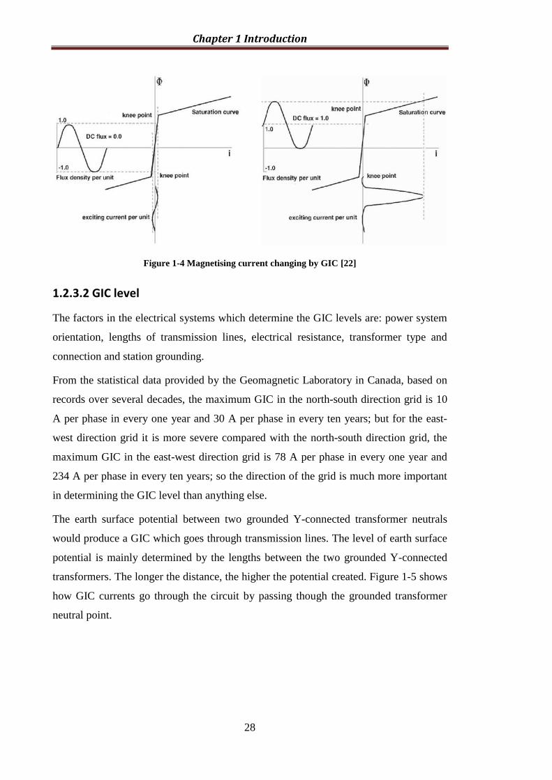
In Figure 1-4, the left side figure shows the approximation of a typical power
transformer excitation characteristic under the normal working condition, and the right
side shows the two straight line piece-wise approximation of a typical power
transformer excitation characteristic under GIC conditions. It can be seen that the
transformer under normal operation works in the linear region of the magnetic
characteristic, and the magnetising current is quite small (normally about 0.5% of the
rated load current). However with GIC, the flux is offset and is driven past the knee area
of the core saturation curve during the positive half-cycle with a large magnetising
current. The transformer works in both the linear and therefore the non-linear regions.
The flux offset for a given GIC magnitude depends on the ultimate slope of the
saturation curve.
Chapter 1 Introduction
28
Figure 1-4 Magnetising current changing by GIC [22]
1.2.3.2 GIC level
The factors in the electrical systems which determine the GIC levels are: power system
orientation, lengths of transmission lines, electrical resistance, transformer type and
connection and station grounding.
From the statistical data provided by the Geomagnetic Laboratory in Canada, based on
records over several decades, the maximum GIC in the north-south direction grid is 10
A per phase in every one year and 30 A per phase in every ten years; but for the east-
west direction grid it is more severe compared with the north-south direction grid, the
maximum GIC in the east-west direction grid is 78 A per phase in every one year and
234 A per phase in every ten years; so the direction of the grid is much more important
in determining the GIC level than anything else.
The earth surface potential between two grounded Y-connected transformer neutrals
would produce a GIC which goes through transmission lines. The level of earth surface
potential is mainly determined by the lengths between the two grounded Y-connected
transformers. The longer the distance, the higher the potential created. Figure 1-5 shows
how GIC currents go through the circuit by passing though the grounded transformer
neutral point.

Chapter 1 Introduction
29
Figure 1-5 Induced voltage drives GIC to/from neutral ground points of power transformers [22]
Due to the earth surface potential, the GIC current is a Quasi-DC low frequency source,
and all the system components are normally modelled by the DC resistance which
include transmission line resistance, transformer winding resistance and grounding
resistance. In addition, all the resistance value would determine the GIC level. Figure
1-6 shows the DC model for one phase. And there must be two Y connection
transformers with a long transmission line for the GIC to occur.
Figure 1-6 DC model for calculating GIC[20]
1.3 Objectives
In the power system network, transformer saturation can cause voltage disturbance
problems and transformer damage or at least the speeding up of insulation ageing
through excessive heating.
Low frequency switching transients such as ferroresonance, inrush currents and what is
now increasingly known as geomagnetic induce currents (GIC), are the most common
phenomena to cause transformer core saturation.
Grounded transformer neutrals
Transmission line
Earth
L
Y
G

Chapter 1 Introduction
30
Although the ferroresonance and the GIC phenomena have been investigated for
decades, there are new challenges because of the improvements in transformer core
materials and lower loss components used in the power system. Besides, the
investigations of these phenomena have increased in recent years due to severe system
and transformer failures.
Most research focuses on individual transformers and the phenomena which cause core
saturation. Transformers were modelled and voltage/current waveforms were analysed.
These studies provided a limited comparison between different types of transformer
installed in the system, and concentrated on a simplified core representation; they did
not fully consider core saturation issues in system studies. Besides, the three-phase
transformer core model still needs further development in order to accurately simulate
the associated problems mentioned before.
With these problems in mind, this research project will develop two main simulation
models: a mathematical transformer magnetic circuit model based on the elementary
magnetic circuit theory; a transient model for the complete network modelling and for
carrying out the low frequency transient study for the interpretation and understanding
of the behaviour of transformers and the interaction between the transformer and the
system. The main objectives of this thesis are outlined below:
1. To build a mathematical transformer magnetic circuit model based on magnetic
circuit models. Taking practical examples of a three-phase three-limb two
winding transformer and a three-phase five-limb auto-transformer for
comparison, to discuss the influence of core structure and core materials; then to
perform sensitivity studies with this model to determine the effect of the model
parameters under balanced and unbalanced situations; thereby to identify the key
parameters of transformers and systems which significantly affect the
phenomena.
2. To identify the correlation between the GIC primary current waveform and the
winding type, core structure type, and the system parameters.
3. To develop a more accurate model of ferroresonance for use in transmission and
distribution systems that not only matches with the field test results but also
identifies the key parameters of the ferroresonance. Based on the system model,
sensitivity studies of different sets of system parameters in combination with the
circuit-breaker grading capacitance, the cable-ground capacitance and the

Chapter 1 Introduction
31
transformer characteristics were carried out, in order to identify how these
parameters influence the ferroresonance phenomena.
1.4 Major contribution and originality
In this research, two simulation models were developed: a mathematical transformer
magnetic circuit model and a transient model.
The flux distribution and magnetising currents were analysed based on the transformer
magnetic circuit model. Moreover, the three-limb core with zero sequence flux return
path transformer magnetic model can be used to deal with the unbalanced situation, and
the fluxes distribution and magnetising currents were analysed.
The low frequency transient studies for the interpretation and understanding of the
behaviour of transformers and the interaction between the transformer and the system
were carried out by using the complete transient network model. And the key influential
parameters were also pointed out.
The achievements of this research are as follows:
1. The influences of core structure and core material on magnetising current
waveform and flux distribution under balanced (normal operation) and
unbalanced (AC+GIC) situations, by using the developed magnetic circuit core
model, were illustrated.
2. The fundamental understanding of GIC and ferroresonance events in the power
networks, by using the ATP model, was established.
3. Among all the influential parameters identified, transformer core structure is the
most important one. The five-limb core is easier to be saturated than three-limb
core under the same GIC events; the smaller the side yoke area of five-limb core,
the easier it will be saturated.
4. More importantly, under GIC events, a transformer core could become saturated
irrespective of the loading condition of the transformer if it is a strong network.
In summary, it helps the industry to understand systemically how GIC influences the
transformer itself, and the system operation. The key parameters identified by the
sensitivity study are: solar storm level, transformer structure, size ratio of side yoke to

Chapter 1 Introduction
32
main yoke for a five-limb transformer and the system impedance which includes
resistance and inductance.
1.5 Thesis outline
This thesis consists of six chapters which reflect the progress of the research in
achieving the objectives previously outlined.
Chapter 1 Introduction: as already noted gives general background and describes the
general structure of the work.
Chapter 2 Basics of transformers: introduces the basic fundamental theory of
transformers, including the transformer core materials, core structure and core losses;
and also the transformer winding structure.
Chapter 3 Literature review: the literature review provides an overview of the power
system transients produced by ferroresonance and GIC conditions and their influence on
networks and network components. A review of the GIC and ferroresonance influence
on the power system and its transformers is also provided. The methodologies of
investigation are reviewed, in terms of modelling and parameter analysis.
Chapter 4 Steady state magnetic circuit modelling for transformers: using
equivalent magnetic circuits to model the transformer core, three-limb and five-limb
transformer core models are represented which include ideal three-limb, three-limb with
return path and five-limb core. All the models were verified for accuracy by using the
manufactures’ test report data. The magnetising currents affected by the core structure
types are discussed and the conclusions are drawn. One GIC case study involved using
the magnetic circuit model and sensitivity studies into the parameter influences were
carried out.
Chapter 5 GIC magnetic and electrical circuit modelling: using ATPDraw
simulation software to simulate the GIC influences on the transformer and to analyse
the current waveforms using Fourier analysis. The theory of the phenomena is given
first. Secondly, further investigation into the influence of the winding and transformer
core structure is discussed. The conclusions are drawn.
Chapter 6 Low frequency switching transient magnetic and electrical modelling:
investigations of de-energisation switching transients were carried out on a 132 kV

Chapter 1 Introduction
33
distribution network in the UK. The current and voltage signals produced by these
operations were fully monitored. They are based on available field data and also circuit
layout diagrams, transformer factory test results, cable design data etc. A simulation
model of this network was built-up and sensitivity studies carried out; certain
modifications were made to the ATP network model for this purpose. The results were
compared with the recorded signals to obtain an understanding of the phenomena
involved. Good agreement between recorded and simulated results was obtained and
some of the main parameters in the process were identified.
Chapter 7 Conclusion and future work: presents the conclusions drawn from this
study and proposals for the future work.

Chapter 2 Basics of transformers
34
Chapter 2 Basics of transformers
2.1 Introduction
In this chapter, the basics of transformer are introduced, in terms of the main
components of transformer structure, i.e. winding and core. Statistical analysis was
conducted on the open-circuit test data of National Grid transmission transformers,
which were built over last four decades with the influence of changes and evolutions of
material and structure. The results are presented in this chapter to illustrate the variety
and complexity of core saturation issue when individual transformer is concerned.
2.2 Transformer structure
A transformer is a device that transfers electrical energy from one circuit to another
through inductively coupled conductors---the transformer’s windings. Primary and
secondary windings are wound concentrically around a transformer core. The major
function of the core is to provide the maximum magnetic coupling between the two
windings, and the major objective for the transformer designer is to try and minimise
the loss of power which includes the core loss and winding loss.
The main components of a power transformer are winding and core.
The main components of a power transformer are winding and core. For the winding
structure type there are disc type and layer type windings. The disc type winding may
be classified as, a continuous disc winding, an inter-shielded disc winding, and an inter-
leaved disc winding, these are normally used for the HV winding [24]. The layer type
winding is less common for HV windings, but more common for low voltage windings
at 11 kV and below, and is also used as the tertiary windings in auto-transformers [4].
For the core structure type there are single-phase core and three-phase core structures,
for single-phase transformers there are three typical core structure types, which are
single phase both limbs wound, single-phase centre limb only wound and single-phase
cruciform [4]; for three-phase core there are two typical core structure types which are
widely used in the UK, they are the three-limb core and the five-limb core. The
transformer core is made up of electric steel laminations, the purpose of which is to

Chapter 2 Basics of transformers
35
reduce eddy current core losses as well as to provide a low reluctance path for the
magnetic flux linking the primary and secondary windings.
2.2.1 Main component---winding
In general, there are categories of three-phase two-winding transformers and three-
phase three-winding transformers. Normally, it is reasonable to have three-phase delta
connected (Δ) windings in a transformer, for delta windings can absorb the third order
harmonic. A two-winding transformer normally uses a star-delta connection, if it is not
an auto-transformer. A three-winding transformer is a star-star-Δ or auto (A)-Δ
connection. The star connection (Y) is generally used on the high voltage side whilst the
delta is used on the low voltage side. The generator step-up transformer usually uses the
Δ-Y connection, the delta side is connected to the generator side and the star side
connected to the transmission side. Then the transmission transformers will have a Y-Y-
Δ or A-Δ connection.
Since National Grid is the operator of the transmission system in the UK, their
transformers are Y-Y-Δ, Y-A-Δ and Y-A (occasionally) connected. As we know, the
existence of the tertiary windings affects the harmonic contents of the magnetising
currents. Figure 2-1 shows the average three-phase magnetising current (The word
magnetising current is equivalent to an open circuit current) value for different
transformer winding connections. In total, twenty one transformers of 275/132 kV, 240
MVA from the National Grid database were selected for the analysis. Seven
transformers are in each group of the same connection.
Figure 2-1 Average magnetising current for different winding connection
For Y-Y-Δ and Y-A-Δ, the 13 kV tertiary winding exists and it is used for the open
circuit test; however in Y-A connection there is no 13 kV tertiary winding, then the
open circuit test would be carried out at 132 kV. In Figure 2-1, the results of Y-A
0
5
10
15
20
25
Y-Y-Δ Y-A Y-A-Δ
Ma
gn
etiz
ing
cu
rren
t (A
)
Connection
Average Magnetizing current for different connection
No Load Current(A) φA No Load Current(A) φB No Load Current(A) φC
Average magnetising current for different winding connections
Mag
ne
tisi
ng
curr
en
t (A
)
Connection

Chapter 2 Basics of transformers
36
connection are normalised and converted from the 132 kV star connections to 13 kV
delta connection results.
2.2.2 Main component---transformer core
As mentioned before, there are two types of core structure which are well used in the
UK; one is a three-limb transformer core and the other is a five-limb transformer core.
For the same capacity transformer, the five-limb core one can be lower in height than
the three-limb core one and it is more convenient to transport; however the core loss is
higher than the three-limb transformer [25].
In order to take full advantage of the circular winding interior space, the lamination-
stacked core cross area is arranged into an approximately circular section. The
transformer manufacturers use different-width laminations to build up the core; however
the width variation depends on the lamination manufacturers. Usually, the width
variation is 10mm. Therefore, the core filling rate of the cross area is around 90% [26].
Due to the fact that the core consists of laminations, the mechanical strength of the
laminations cannot withstand its own weight, so core steel bolts were used in the past to
hold the core laminations together by bolts passing though the limb and the yoke.
However, these holes and bolts would increase the magnetic reluctance in the flow
direction of flux which means it would increase the core loss and, in extreme situations
the flux would find other paths partially outside the transformer core, going through
other metal components in the transformer such as transformer tank, core clamping and
so on. The current reference technology is to use bands of either steel or glass fibre to
hold laminations to the core limb and to use metal-frame clamping structure to hold
laminations to the yoke.
The overlapping of lamination at the joint area is important so that it is able to decrease
or increase the core loss; actually most of the core loss is from the yoke and limb joints.
The 45-degree mitred overlapping is usually used to overlap the lamination in five steps
[10], the more steps there are, the harder it is to build the core ; so the optimal five step
one is chosen mainly due to economics.
The general layout of a three-phase three-limb transformer and the flux in the core are
shown in Figure 2-2 (a) and (b).

Chapter 2 Basics of transformers
37
The L1 and Lm are the effective length of the limb and yoke; Al represents the cross-
section area of the limb and the yoke. The three-phase fluxes for the three-limb core are
indicated by ФA, ФB, and ФC. In the three-limb arrangement, three limbs are wound by
windings which correspond to the three phases. Each limb is joined together by the top
and bottom yoke, which complete the magnetic circuit. One characteristic is that the
cross-section areas of the top and bottom yokes are equal to that of the limb (Al);
therefore, when the transformer works under the linear region in normal working
conditions, the flux in the yoke is equal to the nearby limb; the flux through each limb is
sinusoidal since the voltages applied across the winding are sinusoidal. Ideally, as long
as the fluxes are at the same magnitude and their phase angles are electrically 120° apart,
the fluxes will cancel each other in the top and bottom yokes. Consequently, for applied
three-phase balanced voltages, no flux return path is required [26]. However, if there is
the unbalanced voltage component, the flux has to travel along a high-reluctance path
through a very long air gap and come back to the core again.
ΦA ΦB ΦC
(-ΦA)
(-ΦC)
(-ΦC)
(-ΦA)
Lm
Ll
Al
(a) (b)
Figure 2-2 Three-phase three-limb core type transformer
The general layout of a three-phase five-limb transformer and the flux in the core are
shown in Figure 2-3 (a) and (b). As in the three-phase three-limb core, the effective
length of the limb is denoted as Ll. The main yoke and side yoke effective lengths are
indicated by Lm and Ls respectively. The cross-sectional area of the side yoke is given as
the main yoke, while the cross-section areas for the main limb and the main yoke are
taken as Al and Am. The three main centre limbs carry three-phase fluxes ФA, ФB, and
ФC. Фls and Фrs represent the fluxes at the side yokes.
In a five-limb transformer, the three-phase windings are wound on the middle three
limbs similar to a three-limb transformer, the difference is that there are two extra limbs,

Chapter 2 Basics of transformers
38
one on each side of the three main limbs, and the cross-section areas are smaller than
those of the main limbs. The cross-section of the main yoke is not equal to, like the
three-limb transformers, but smaller than the main limb cross-section area. These two
side yokes are for carrying extra flux when the transformer meets the unbalanced
situation or the main yoke cannot carry more flux, without going into saturation.
The flux variation in the main and side yoke of five-limb core was investigated by
English Electric Company Limited and was reported in October 1968 in order to
evaluate the iron losses [26]. It was discovered that the fluxes in the yoke and side
yokes are non-sinusoidal because the flux in a main limb has two alternative paths when
flowing into the yoke, neither of which is pre-determined.
Core Yoke AB
Core Limb A
Winding Set A Winding Set C
Core Limb B Core Limb C
Core Yoke BC
HV Winding LV Winding
Side Yoke
Side Limb Side Limb
Side Yoke
(a)
ΦA ΦB ΦC
(ΦAB)
(ΦBC)
(ΦBC)
(ΦAB)Lm
Ll
Al
Ls
Am As
(Φls) (Φrs)
(b)
Figure 2-3 Three-phase five-limb transformer core
Comparisons of the magnetising currents were made of the two types of transformer
core structures operated by National Grid UK, which are three-limb and five-limb core
type transformers. Due to the structural difference, the magnetising currents are

Chapter 2 Basics of transformers
39
different for the three-limb and five-limb core. As mentioned earlier, the magnitudes of
the magnetising currents are mainly determined by the magnetising loop length if the
core materials used are the same. However, the transformers selected used different
materials to build the cores so the magnitudes of the open circuit currents cannot be
compared without being normalised.
Figure 2-4 shows the results of the three-phase average magnetising current for two
different core structures under the same voltage level and same power rating. One phase
current of the lowest value is regarded as per unit base. There are eight three-limb and
eight five-limb transformers examined, which are picked up from the same 400/275 kV
voltage level and 1000 MVA power rating.
Figure 2-4 Average magnetising current in per unit for different core structure
The open circuit current values for the three phases show that the unbalanced situation
in terms of the magnitudes of the magnetising currents of the five-limb core is greater
than that of the three-limb core. In other words, the ratio between the yoke length and
the limb length of the transformer core, and the area ratio, yoke area to limb area, of
transformer would determine the unbalanced situation.
2.2.3 Transformer core materials
There are three different types of magnetic materials which are diamagnetic materials,
paramagnetic materials and ferromagnetic materials [27].
Ferromagnetic materials, which have a large and positive susceptibility to an external
magnetic field, are widely used to build power transformers.
1.00 1.00
1.12
1.02
1.42
1.23
0
0.2
0.4
0.6
0.8
1
1.2
1.4
1.6
3-limb 5-limb
Ma
gn
etiz
ing
cu
rren
t (p
.u.)
Core structure
Average magnetizing current for different core structure
No Load Current(A) φA No Load Current(A) φB No Load Current(A) φC
Average magnetising current for different core structures
Mag
ne
tisi
ng
curr
en
t (p
.u.)
3-Limb 5-Limb
Core structure

Chapter 2 Basics of transformers
40
In order to build a transformer, we need the transformer core to provide low reluctance
and high permeability. So the ferromagnetic materials are suitable for the transformer
core construction. However, the hysteresis loop is one of the important characteristics of
the magnetic properties of ferromagnetic materials. A hysteresis loop shows the
relationship between the induced magnetic flux density (B) and the magnetising force
(H). It is often referred to as the B-H loop. The voltage supply corresponds to B and the
magnetising current corresponds to H, due to H*l = N*I (l is the magnetic loop length,
N is the turn number, I is the magnetising current). There are two ways to represent the
characteristics of the material which are the B-H curve (hysteresis loop) and the
Lambda-I curve (lambda is the total flux in the transformer core).
Superficially, the transformer core structure has not been through great changes,
although small changes have been made and designers have been constantly working to
reduce core losses. The core loss at specified frequency includes two parts: the first is
hysteresis loss which is dependent on the area of the hysteresis loop, and the second is
eddy current loss which is dependent mainly on the thickness of the material. The
components of core loss are represented by these equations:
Hysteresis Loss: 1 max ( / )n
hW k fB W kg
Eddy current Loss: 2 2 2
2 / ( / )e effW k f t B W kg
where k1 and k2 are constants for the material
f is the frequency, Hz
τ is the thickness of the material, mm
ρ is the resistivity of the material, Ω∙m
Bmax is the maximum flux density, Tesla
Beff is the flux density RMS value of the applied voltage, Tesla
n is the ’Steinmetz exponent’ which is a function of the material [28].
When a ferromagnetic material is magnetized in one direction, it will not relax back to
zero magnetization when the imposed magnetising field is removed. It must be driven
back to zero by the opposite source. If an alternating magnetic field is applied to the
material, its magnetization will trace out a loop which is called hysteresis loop. The area
enclosed by this loop is proportional to the hysteresis loss.

Chapter 2 Basics of transformers
41
Normally the hysteresis loop can be separated into three parts being the linear region,
knee region and non-linear region. For all the transformers, the designer tries to use the
minimum material to transfer maximum energy from primary to secondary windings, so
the aim is to ensure that, in operation, the flux excursions do not pass through and
beyond the knee point. In this region the relative permeability of the material is still at a
high level which is around 6000 or more depending on the core material [29].
The early transformer cores were made from high-grade wrought iron; however it was
recognised that the addition of small amounts of silicon or aluminium to the iron greatly
reduced the hysteresis losses, increased permeability and also increased the resistivity,
which also resulted in reduced eddy current losses [4]. Table 2-1 shows that as
transformers evolved at different stages of development, different materials were used
for the transformer core application.
Table 2-1 Historical development of the core steels [4]
Steels Types Period Losses
(@ 1.5 T, 50 Hz) Usage
Hot-rolled Steels Until 1940s 7 W/kg /
Cold-rolled Steels
(Grain-oriented steel)
1940s-
1960s 1.5 W/kg
Early transformer
production in
general usage
High Permeability Steels 1965s-Now
1 W/kg (Reduction of
30-40% in hysteresis
loss)
Early transformer
production in power
transformer usage
Domain Refined Steels 1983s-Now 0.85W/kg (@1.7 T) Newer transformer
in general usage
Amorphous Steels 1970s-Now 0.28 W/kg
Where very low
core loss is
required; costly
Microcrystalline Steels / 0.56 W/kg (@1.7 T) /
Figure 2-5 shows the general comparison between the characteristics of the modern
materials and the characteristics of the old materials.

Chapter 2 Basics of transformers
42
Figure 2-5 Ferromagnetic material hysteresis loop [30]
The left side of the figure shows the characteristics of the modern materials and the
right side shows the characteristics of the old materials. It can be seen that the modern
materials have fewer losses compared to those of the old materials. Also, the maximum
flux density can reach much higher values in the modern materials. The knee point for
the modern materials is also higher, being around 1.7 T, whereas for the older materials
it is only 1.4 T [29].
The high permeability grain-oriented and the domain refined steels have a better
orientation compared with conventional steel; and also that at flux densities of 1.7 T and
higher, that permeability are three times higher than that of the best conventional steel,
and the stress sensitivity of loss and magnetostriction is lower. However, the magnitude
of the eddy current loss of conventional and the new material are very similar [31].
There are three factors which would influence the magnetising currents, and they are the
core steel material, core structure and winding connection.
Statistically the test reports of transformers serving in the National Grid were analysed.
They are of 400/275/13 kV, 400/275 kV, 275/132/33 kV, 275/132/13 kV or 275/132 kV,
being examined in terms of the open circuit test current of three phases. The test reports
showed the existence of the differences of three-phase open circuit currents all
transformers. Comparison was also made on the transformers manufactured at different
years. For different decades, the manufactures might use different types of material for
the transformer core. The magnitude of the magnetising current is determined by the
core material subject to the same building method. Figure 2-6 shows the open circuit
current distribution versus the transformer designs from the 1960s to 2000s.
New materials Older materials

Chapter 2 Basics of transformers
43
Figure 2-6 Average magnetising current of different installation year of transformers at 400/275/13
kV and 1000 MVA
The columns in red, yellow and blue of the figure represent the magnetising currents of
phase A, B and C. It can be seen that overall the data of the 1990s is lower than the data
of the 1960s. As mentioned before, the cold-rolled steels (Grain-oriented steel) were
used as transformer core material in the 1960s. Afterwards, not only were newer
materials produced for core material in order to reduce the hysteresis losses such as high
permeability steels, domain refined steels and amorphous steel, the production process
was also improved, to further reduce the losses of the core steel.
Figure 2-7 (a) shows that the improvement in magnetic properties over the past 80 years
[31]; and (b) is the survey made in the research work on the magnetising currents from
the manufactures’ test reports of 400/275/13 kV, 1000 MVA transformers in National
Grid. It can be seen that as the improvement of the material’s characteristics, both the
material loss and the permeability characteristics improve.
0
5
10
15
20
25
30
35
1968 1972 1973 1976 1986 1987 1991 1992 1992 1992 1993 1995 1996 1997 1998 1998 1998 2001 2001 2001
Ma
gn
etiz
ing
cu
rren
t (A
)
Year
Magnetizing current for 1000MVA
No Load Current(A) φA No Load Current(A) φB No Load Current(A) φC
Newer core steelsOlder core steels
Magnetising current for 1000MVA transformers
Mag
ne
tisi
ng
curr
en
t (A
)
Year
(a) [31]

Chapter 2 Basics of transformers
44
Figure 2-7 Losses and magnetising currents from year to year
0
10
20
30
40
50
1960 1965 1970 1975 1980 1985 1990 1995 2000 2005
Cu
rre
nt(
A)
Year
Magnetizing current for different year
(b)
Magnetising current for different years

Chapter 3 Literature review
45
Chapter 3 Literature review
3.1 Introduction
This chapter provides a literature review on the transient studies of the system network,
in particular, switching ferroresonance transients and GIC phenomena. Both are
associated with transformer core saturation problems. Background knowledge was
acquired on how to understand the reasons for the ferroresonance phenomena and the
geomagnetic induce current phenomena are also introduced; the investigation methods
are summarised and the mitigation methods are also relayed in this chapter.
Generally, the transient phenomena would be separated into different frequency ranges
from DC to about 50MHz. The transient phenomena appear as transitions from one
steady state condition to another. The primary cause of such disturbances in a system
are closing or opening of a circuit breaker or another switching equipment, short-
circuits, earth faults or lightning strokes.
Table 3-1 shows the overview on the different causes of transient phenomena and their
most common frequency ranges [1].
Table 3-1 Cause of system transients and frequency ranges [1]
Cause Frequency Range
Transformer energisation 0.1 Hz - 1 kHz
Ferroresonance
Load rejection 0.1 Hz - 3 kHz
Fault clearing 50/60 Hz - 3 kHz
Fault initiation 50/60 Hz - 20 kHz
Line energisation 50/60 Hz - 20 kHz
Line reclosing 50/60 Hz - 20 kHz
Transient recovery voltage 50/60 Hz - 20 kHz
Terminal faults 50/60 Hz - 20 kHz
Short line faults 50/60 Hz - 100 kHz
Multiple re-strikes of circuit breaker 10 kHz - 1 MHz
Lightning surges, faults in substations 10 kHz - 3 MHz
Disconnector switching and faults in GIS 100 kHz - 50 MHz
From this table, we can see that, the frequency range of transformer switching transient
is around 0.1Hz to 1 kHz, which belongs to the low frequency range. The CIGRE
working group classified the frequency range of the system transients into four different
groups [1]. The switching transients and the GIC all belong to the low frequency range.

Chapter 3 Literature review
46
3.2 Power system operation transient---switching
transients
3.2.1 Background
Switching transients are the most frequently occurring transient phenomena in the
power system. The system network needs maintenance, capacitor bank switching,
energisation of the loads and transformers and also the new network synchronization
such as the wind farm and so on; all of those operations would cause switching
transients.
For the transformers, two main switching transient phenomena would occur which are
magnetising current inrush when a transformer is switched on to the network; and
ferroresonance when the transformer is switched off at off-load or light-load condition.
Ferroresonance is one of the core saturation phenomena which could cause overvoltages
and overcurrents at the terminals of a transformer. Besides overvoltages and
overcurrents, when the core saturates, the overfluxing issue can also cause local
overheating of transformer insulation [32]. Overfluxing possibly include two definitions:
one is when core lamination goes into the saturation region of the λ-I curve, the other is
when the flux leaks out of the joint area and goes into the insulation/metal clamping
frame area.
Inrush is another phenomenon where a transformer can be pushed into the deep
saturation, and the maximum magnitude value of the current value can achieve several
times the nominal load current. During the period of inrush the iron loss and copper loss
are extremely high.
Electric stress on transformer insulation caused by overvoltages, and thermal stress
caused by overheating and overcurrents, can result in transformer failures. This is one of
the main reasons why a network operator is worried about the ferroresonance and inrush
phenomena.

Chapter 3 Literature review
47
3.2.2 Ferroresonance
3.2.2.1 Background
Ferroresonance is defined as the steady-state mode of operation that exists when an
alternating voltage of sufficient magnitude is applied to a circuit consisting of
capacitance and ferromagnetic inductance which are repeated each half cycle [33].
Ferroresonance is an old topic and there are substantially large volumes of literature
studying this practical phenomenon experienced by transmission & distribution
networks upon state-changing events such as switching or fault operations. The first
published work, which simply defined the ferroresonance phenomenon as transformer
resonance, was written by J.Bethenod in 1907 [34]. The word ferroresonance was first
used in the 1920s by P.Boucherot [35] to describe the series resonance involving
capacitance and nonlinear inductance of the transformer core. It was in the 1930s that
the subject of ferroresonance generated practical interest when the use of series
capacitors for voltage regulation caused ferroresonance in distribution systems [36],
resulting in damaging overvoltage. The first analytical work was presented by
Rüdenberg in the 1940s [37] and in the 1950s a more detailed analytical work was
completed by Hayashi [38].
Ferroresonance can be split into sustained and transient ferroresonant phenomena;
sustained ferroresonance has the power system acting as the supply source for the
resonating phenomenon; for example via inter-circuit overhead lines a no-load
transformer is supplied by the power system and it is possible to have sustained
ferroresonance [14, 39]; the overvoltage can be sustained for a long time. [40] described
the sustained fundamental mode and sub-harmonic mode of the ferroresonance in the
real network in the UK. On the other hand the transient ferroresonance phenomenon is
normally supplied by a limited energy source such as a capacitor made of a length of
cable, after a switching operation which isolates part of the network. [12] gave an
example about the transient ferroresonant experience, where the limited energy stored in
the cable is transferred between the cable and the saturated transformer; the transfer
continues until system losses have absorbed all the energy.
A special publication on the Practical Aspects of Ferroresonance [11] has been written
by the IEEE Working Group on “modelling and analysis of systems transients using

Chapter 3 Literature review
48
digital programs”. One of the tasks of the Working Group is to provide a comprehensive
survey of the ferroresonance issues reported in the literature.
According to [11], 129 papers are reviewed and categorised as practical, including
seven different classes of ferroresonant circuits, which are
1) Transformer accidentally energised on one or two phases
2) Transformer energised through the grading capacitance of one or more open
circuit breakers
3) Transformer connected to a series compensated transmission line
4) Voltage transformer connected to an isolated neutral system
5) Capacitor voltage transformer
6) Transformer connected to a de-energised transmission line running in parallel
with one or more energised lines
7) Transformer supplied through long transmission lines or cables with low short-
circuit power.
All the circuits above must contain at least: a non-linear inductance (ferromagnetic and
saturable), a capacitor, a voltage source (generally sinusoidal) and low losses. The
initiation of ferroresonance needs some types of switching event such as load rejection,
fault clearing or single phase switching or loss of system grounding.
The same IEEE Working Group also produced a paper focusing on analysis and
modelling guidelines for slow transients, i.e. the study of ferroresonance [41]. A
comparison between single-phase and three-phase transformer modelling was carried
out for ferroresonance. The three-phase system cannot be modelled accurately by using
per phase simulation, due to the transformer core configuration and winding connection.
A complete three-phase model needs to be used. It is also mentioned that to represent
the transformer core, the core configuration must be considered and the saturation
characteristic must be accurately modelled [42]. Circuit breaker opening time and
sequence also play an important role for ferroresonance.
In the power system, saturable inductances can exist in the form of power transformers,
voltage measurement inductive transformers (VT) and shunt reactors; for capacitances,
there are cables and long transmission lines, capacitive voltage transformers, series or
shunt capacitor banks, and voltage grading capacitors in circuit-breakers and so on. A
ferroresonance phenomenon is more likely to be created with minimal load or a low
level of damping, and for unbalanced 3-phase excitation with coupling between phases,

Chapter 3 Literature review
49
or between circuits of double-circuit lines. Besides, the initial conditions of capacitor
and inductor also influence the ferroresonance phenomena such as: the level of residual
flux in the magnetic core and the initial charge on the capacitive components [43].
The consequences of ferroresonance can be untimely tripping of protection devices (due
to overvoltages and overcurrents) and destruction of equipment such as power
transformers or voltage transformers (overvoltages, overcurrents and overfluxing).
3.2.2.2 Ferroresonance effect on transformer
Ferroresonance phenomena often occur during normal circuit operation and circuit
faults in the power system; some cases happen due to the grading capacitance
transferring energy to transformers or inductive components, some are due to the
coupling capacitance between two circuits transferring energy to transformers or
inductive components, and some are due to the ground capacitance transferring energy
to transformers or inductive components; but the fundamental theory underlying these
phenomena are quite simple; because there are non-linear inductance and capacitance in
the network, and during the circuit reconfiguration the energy from capacitance would
discharge to non-linear inductance and furthermore push the transformer into saturation,
and depending on the resistance value of network, the ferroresonance would display in
two ways: one is the sustained mode due to low loss; the other one is the decayed mode.
Most of the case studies were carried out via field tests or using network modelling to
investigate ferroresonance phenomena, those researchers focused on the network level
in the study of transient phenomena. However, not only are overvoltages and
overcurrents experienced by transformers during ferroresonance, but overfluxing can
also occur [32], and the associated local overheating is regarded as one of the long-term
ageing factors. When ferroresonance events happen, the core must be saturated, and it
would cause the relative permeability of the iron core to decrease from the linear region,
which is several thousands, to that of saturation region, which is only tens [44]; the flux
would leak out from the core to the clamping frame, oil and other components inside the
transformer tank or even the tank which could produce more local heating of these
components.
The eddy current loss is not only dependent on the square of frequency but is also
directly proportional to the square of the thickness of the material. Since the laminations
of transformer core are produced by using a special process, the thickness is much
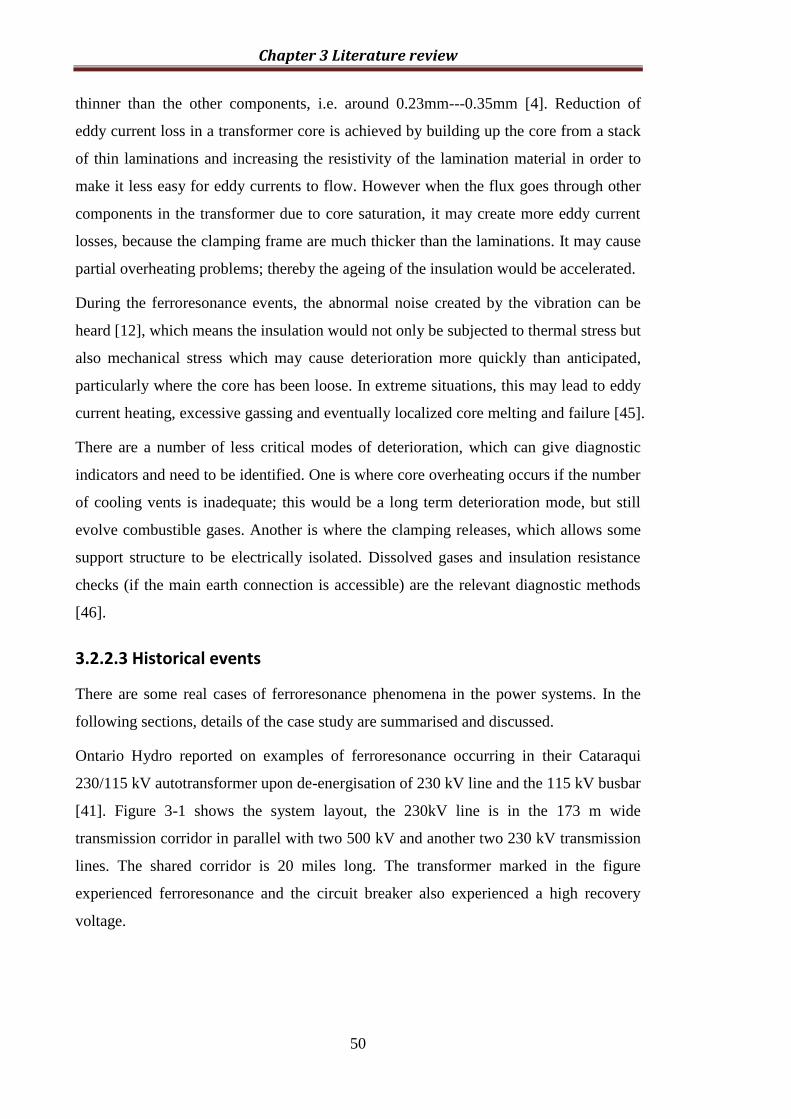
Chapter 3 Literature review
50
thinner than the other components, i.e. around 0.23mm---0.35mm [4]. Reduction of
eddy current loss in a transformer core is achieved by building up the core from a stack
of thin laminations and increasing the resistivity of the lamination material in order to
make it less easy for eddy currents to flow. However when the flux goes through other
components in the transformer due to core saturation, it may create more eddy current
losses, because the clamping frame are much thicker than the laminations. It may cause
partial overheating problems; thereby the ageing of the insulation would be accelerated.
During the ferroresonance events, the abnormal noise created by the vibration can be
heard [12], which means the insulation would not only be subjected to thermal stress but
also mechanical stress which may cause deterioration more quickly than anticipated,
particularly where the core has been loose. In extreme situations, this may lead to eddy
current heating, excessive gassing and eventually localized core melting and failure [45].
There are a number of less critical modes of deterioration, which can give diagnostic
indicators and need to be identified. One is where core overheating occurs if the number
of cooling vents is inadequate; this would be a long term deterioration mode, but still
evolve combustible gases. Another is where the clamping releases, which allows some
support structure to be electrically isolated. Dissolved gases and insulation resistance
checks (if the main earth connection is accessible) are the relevant diagnostic methods
[46].
3.2.2.3 Historical events
There are some real cases of ferroresonance phenomena in the power systems. In the
following sections, details of the case study are summarised and discussed.
Ontario Hydro reported on examples of ferroresonance occurring in their Cataraqui
230/115 kV autotransformer upon de-energisation of 230 kV line and the 115 kV busbar
[41]. Figure 3-1 shows the system layout, the 230kV line is in the 173 m wide
transmission corridor in parallel with two 500 kV and another two 230 kV transmission
lines. The shared corridor is 20 miles long. The transformer marked in the figure
experienced ferroresonance and the circuit breaker also experienced a high recovery
voltage.

Chapter 3 Literature review
51
Figure 3-1 Ontario Hydro 230kV System [41]
In [47] experts from Manitoba Hydro and Ontario Hydro stated that the close coupling
of parallel circuits with similar or higher voltage increases the risk of ferroresonance in
the disconnected transformers. Based on system configurations of Dual Element Source
Network (DESN) stations, it is shown that 59 km of parallel 230 kV and 32 km of
parallel 500 kV transmission lines were sufficient to cause ferroresonance in a 230/115
kV transformer (auto connected transformer), the circuit configuration is shown in
Figure 3-2.
Figure 3-2 Multi-Voltage transmission circuit [47]
X3H
X4H
X552A
14.25ml. 5.75ml.
X2H
X1HLENNON 500
LENNON 230
KINGSTONGARDINER TS
HINCHINBROOKE TS
16
.57
ml.
TO HAWTHORNE 500 TS
CATARAQUI TS

Chapter 3 Literature review
52
In [13] a three-phase 1000 MVA 525/241.5 kV Y-connected bank of autotransformers,
located at the Big Eddy Substation of Bonneville Power Administration (BPA) in Dallas,
Oregon, is connected to the 525 kV side through a disconnecting switch to 30.5 km of
line and a circuit breaker located at John Day Substation. A local circuit breaker is
provided on the 230 kV bus at Big Eddy. Parallel and on the same right-of-way is the
525 kV John Day-Oregon City line which is shown in Figure 3-3.
Figure 3-3 525 kV transmission system between Big Eddy and John Day [13]
In [14], a 400 kV circuit was identified as a suitable circuit that could be induced into
ferroresonance and tests were planned to examine the disconnector’s capability of
quenching the ferroresonance. The purpose of the tests was to first establish the
likelihood of the occurrence of ferroresonance on SGT 1 shown in Figure 3-4. There is a
parallel overhead line circuit, the coupling distance is 37 km and the feeder has a 1000
MVA 400/275/13 kV power transformer (auto connected transformer). This circuit is
susceptible to ferroresonance when a series of switching operations are carried out in
the following way: the disconnector X303 and the circuit breaker T10 are opened. All
the disconnectors (X103, X113) and circuit breaker X420 connecting to busbar 2 are in
service. The circuit is reconfigured by the opening circuit breaker X420. On SGT 1
ferroresonance would occur.

Chapter 3 Literature review
53
Figure 3-4 Single line diagram of the Brinsworth/Thorpe Marsh circuit arrangement [14]
[16] was published by Jacobson D.A.N. in 1995, the ferroresonance occurred in Dorsey
HVDC converter station, where 230 kV ac bus is comprised of four bus sections on
which the converter valves and transmission lines are terminated. The configuration of
the circuit is shown in Figure 3-5. Firstly, bus A2 was removed from service to
commission replacement breakers, current transformers and to perform disconnects
maintenance and trip testing. After approximately 25 minutes, a potential transformer
(PT) failed catastrophically causing damage to equipment up to 33 m away. The
switching procedure resulted in the de-energised bus and the associated PTs being
connected to the energised bus B2 through the grading capacitors (5061 pF) of nine
open 230 kV circuit breakers. A station service transformer, which is normally
connected to bus A2, had been previously disconnected. A ferroresonance condition
caused the failure of one PT.
Figure 3-5 Main circuit components in Dorsey Converter Station [16]
SGT1
Thorpe Marsh
400 kV
T10 OPENX303 OPEN
Brinsworth
275 kV
SGT2
X420 POW
Switching
Cable 170 m
Cable 170 m
X103
CLOSED
X113
CLOSED
Transmission Line-Side A
Transmission Line-Side B
Dorsey Converter Station Bus
B2 A2
Equivalent source:
Z1=0.212+j*4.38 Ω
(12000 MVA)
Z0=0.307+j*0.968 Ω
Grading
Capacitance
(325-7500 pF)
SST
PT1
PT2
AC filters
(755 MVAr)
Bus
Capacitance
matrix
Stray Capacitance
(4000 pF)

Chapter 3 Literature review
54
Literature [48] described a ferroresonance phenomenon in a 12 kV distribution feeder
connected to a station service transformer (Dyn connected transformer) and
underground cable terminated with riser pole surge arrester. The circuit and the surge
arrester exploded are shown in Figure 3-6. Ferroresonance circuit was formed when
switching operations were carried out by firstly transferring the customer loads to
another feeder via closing the tie switch, secondly opening the circuit breaker which is
the one yellow marked at the feeder and finally opening the disconnector switch.
Figure 3-6 A simplified one line diagram in which the riser surge arrester Riser pole exploded [48]
The incidence of MOV arrester explosion quoted in [17] is concerned with a shopping
mall supplied by a 34.5 kV distribution system via cable-connected pad-mounted
transformer (Dyn connected transformer). The root cause of the occurrence of
ferroresonance is that one of the lines connected to the cable was open as a result of an
automobile accident which is shown in Figure 3-7. This in turn reconfigured the
network into ferroresonance susceptible circuit consisting of the line and cable
capacitance in series with the transformer core.
BAY2BAY1
Substation
BUS 2BUS 1
Opened
CB
Station Service
Transformer
112.5 kVA
350 m. Underground Cable
Arrester
9 kV. 10 kA
Disconnector
Switch
Loads
Tie S
witch
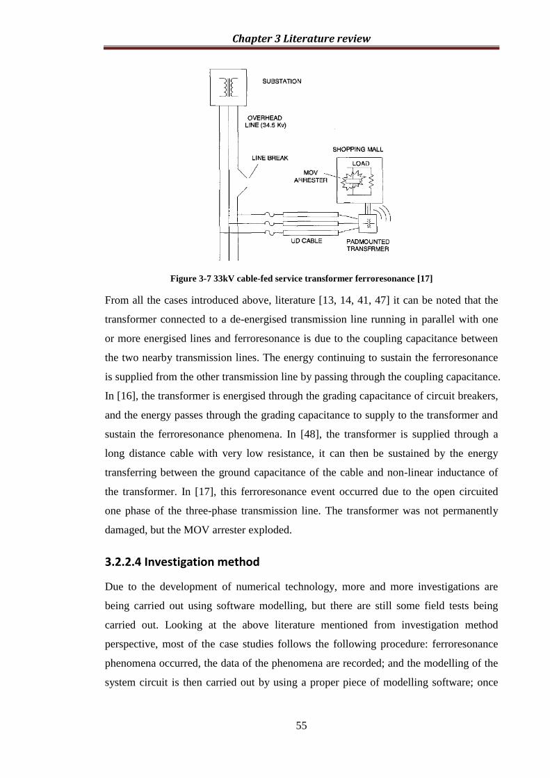
Chapter 3 Literature review
55
Figure 3-7 33kV cable-fed service transformer ferroresonance [17]
From all the cases introduced above, literature [13, 14, 41, 47] it can be noted that the
transformer connected to a de-energised transmission line running in parallel with one
or more energised lines and ferroresonance is due to the coupling capacitance between
the two nearby transmission lines. The energy continuing to sustain the ferroresonance
is supplied from the other transmission line by passing through the coupling capacitance.
In [16], the transformer is energised through the grading capacitance of circuit breakers,
and the energy passes through the grading capacitance to supply to the transformer and
sustain the ferroresonance phenomena. In [48], the transformer is supplied through a
long distance cable with very low resistance, it can then be sustained by the energy
transferring between the ground capacitance of the cable and non-linear inductance of
the transformer. In [17], this ferroresonance event occurred due to the open circuited
one phase of the three-phase transmission line. The transformer was not permanently
damaged, but the MOV arrester exploded.
3.2.2.4 Investigation method
Due to the development of numerical technology, more and more investigations are
being carried out using software modelling, but there are still some field tests being
carried out. Looking at the above literature mentioned from investigation method
perspective, most of the case studies follows the following procedure: ferroresonance
phenomena occurred, the data of the phenomena are recorded; and the modelling of the
system circuit is then carried out by using a proper piece of modelling software; once

Chapter 3 Literature review
56
the model is verified by the recorded data, then more case studies based on this
validated model, such as the parameters sensitivity studies, would be carried out.
In literature [41], the circuit was simulated by using EMTP. There are 18 transmission
lines coupled with one another which included two double-circuit 230 kV lines, and an
existing 500 kV line, and a future 500 kV line. The sensitivity simulation study was
carried out by changing the value of the resistive load so as to understand the situation
once the 115 kV circuit breaker is opened. Results show that the damping resistance (i.e.
load) can work quite well for damping the ferroresonance but it will worsen the
recovery voltage on the circuit breaker.
In literature [47], the model of the circuit was built in EMTP software and the analysis
is from the system operation point of view i.e. protection of the facilities in the power
grid to discuss the reconfiguration by the switching. Six potential phenomena were
discussed which included voltage unbalanced problems, residual load voltage problems,
ferroresonance problems, breaker recovery voltage problems, ground switch duty
problems and working ground problems. The mitigation method for each of those issues
has been concluded.
In literature [13], when the Big Eddy line was being prepared for line maintenance,
immediately before the line was de-energised, the transformer was connected to a load
which was 170 MW real power and 140 MVAR reactive power at the 230-kV bus. The
switching sequence was to first open the 525-kV circuit breaker at John Day, leaving
the transformer bank connected to the line. Secondly, 230-kV circuit breaker at Big
Eddy was opened. Nine minutes later the gas accumulation alarm relay operated on the
C-phase transformer and ferroresonance was estimated to last for about 5 minutes, but it
did not cause the transformer failure. The DGA test was conducted on the transformer
oil and Table 3-2 shows the gas analysis after the occurrence of the ferroresonance.
However, Table 3-2 does not give the gas volume in ppm and the sum of percentage of
the gases is not equal to 100%, nevertheless the main gases are carbon monoxide and
hydrogen.
Table 3-2 Dissolved gas analysis of the transformer [13]
Gas Type Content percentage
Hydrogen 22.2%
Methane 3.3%
Acetylene 0.2%
Carbon monoxide 32.0%
Carbon dioxide 10.0%

Chapter 3 Literature review
57
Through the dissolved gas analysis it was concluded that when the transformer is in
ferroresonance condition it is subjected to the issue of local overheating of parts by the
stray flux when the core is saturated, and also due to the overvoltage in ferroresonance
the transformer oil had the problem of partial discharge [49].
This heating may not cause serious damage in a few minutes but probably will do so if
the ferroresonance is allowed to continue being sustained without detection. The
simulation was carried out by using an electronic differential analyser (EDA) which is
an analog simulation method. Figure 3-8 shows the equivalent circuit of the
ferroresonance circuit. This ferroresonance occurred mainly due to the transmission line
coupling capacitance which can make the energy pass through to the disconnected
transformer.
Figure 3-8 Equivalent circuit of the transformer with the transmission lines [13]
In literature [14], the simulation analysis was carried out by using ATPDraw software.
The model is very similar to that in [13]; there are two main components which are the
coupling capacitance between the transmission line and the non-linear inductance of the
transformer. And the sensitivity studies were carried out by varying the transmission
line length and the switching time to look into their influence on the peak value of the
ferroresonance voltages and currents. The results show that the ferroresonance is a
stochastic function which really depends on the initial condition and the parameters in
the circuit system. In literature [32, 45], investigation of this case is continued; the finite
element model of the transformer was built in the attempt to understand the situation
inside the transformer. It was found that during the ferroresonance, the transformer
saturated in a cyclic way at different parts and the flux would be distorted; it is more
severe at the core bolt area, which would create the localized overheating of the core
bolt area.

Chapter 3 Literature review
58
And again in literature [16], it also used EMTP software to build the network model and
did the analysis at the system level and a mitigation method was given in this paper.
This ferroresonance occurrence is mainly because of the high grading capacitance value
of the SF6 circuit breakers and the energy can pass through the grading capacitance to
the transformers PT1 and PT2. The ferroresonance has two periods; one is the chaotic
mode which is determined by the breaker opening times, pre-switch voltage and the
exact values of all parameters in each phase; the other one is the steady state
fundamental mode and the overvoltage achieves 1.3 per unit of the normal peak value.
In literature [48], there is a surge asserter connected in the circuit; as we know that the
function of the surge asserter is to protect against the overvoltage; however the
overvoltage created by the ferroresonance occurred in such a way that, due to the
amount of energy passing through, the surge asserter is exploded. Two comparison field
tests were carried out by using the same circuit configuration but with two different
conditions, one having arresters installed and the other having no arresters. For the case
that had no arresters, the chaotic mode ferroresonance and sub-harmonic mode
ferroresonance occurred, having a 4.14 per unit and 2.69 per unit peak overvoltage
respectively. For the case that had arresters, only the fundamental mode ferroresonance
appeared with only 1.5 per unit peak overvoltage, but after around 30 seconds the
arrester of the one-phase exploded. This is due to the high energy and lower voltage of
the sustained ferroresonance passing through the arrester but without becoming fully
conductive.
3.2.2.5 Mitigation
There are several mitigation methods used widely in the power system to minimise
ferroresonance overvoltages and overcurrents.
In [41], due to the several transmission lines nearby, the coupling capacitor would
facilitate the occurrence of ferroresonance in one of the substations. In the mitigation
method used, a damping resistance load is added at the secondary of the transformer as
well as surge arresters to control the overvoltages.
In [47], the same reason as in [41], that transmission line capacitance coupling would
bring the transformer into ferroresonance; and in this paper there are several mitigation
methods proposed, which add resistance to the secondary of the transformer as the same

Chapter 3 Literature review
59
as that mentioned in the previous paper, add an individual circuit breaker instead of the
disconnector and use ground switching to pass all the energy through to the earth.
In [16], since the circuit breakers are upgraded from vacuum to SF6 circuit breaker, then
the grading capacitance would achieve up to 7500 pF. The high value grading
capacitance would allow the energy passing through from the source side to the
disconnected side and then the ferroresonance phenomena would occur. For the
mitigation of this case study, a 200 Ohm/phase damping resistor is installed on the
secondary side of the station service transformer to eliminate ferroresonance for faulted
and un-faulted bus clearing.
In [13], several mitigation methods were suggested which include transposing the
parallel transmission lines and reducing the coupling capacitance value; adding damping
resistance to decrease the trapped charge on the line; providing a delta winding for the
transformer for the zero-sequence current and trapping harmonics; grounding the Y-
connected HV windings through a resistor or closing the delta-connected tertiary
windings through a resistor; short-circuit any set of transformer windings; and adding a
circuit breaker to disconnect the transformer from the line. Adding a tertiary winding is
not an economical solution, but adding a switching resistance is the most economical
method to mitigate the ferroresonance. And the simplest and surest way to prevent
ferroresonance is to disconnect the transformer from the line soon after disconnecting
the transformer and line from the rest of the power system.
In [48], two mitigation methods were presented. First, the procedure of the switching
sequence, which is alternated between the circuit breaker and the disconnector switch, is
changed. This solution was proved by field tests and has no extra cost. Secondly, a
resistance load can be applied to the secondary side of the transformer, since the
resistance can dampen the energy, and in this case if the resistance load is more than 1%
of the transformer rated load, the ferroresonance can be avoided.
In [17], a few mitigation methods were given such as, installing a three-phase circuit
breaker at the front of the transformer; ensuring the transformer is loaded while being
switched off; and opening the three-phase circuit breaker simultaneously.
To summarize the mitigation methods in the literature; several common methods are
proposed which are: adding a damping resistance to damp the ferroresonance
phenomena in a short period, controlling the circuit breaker opening time in order to

Chapter 3 Literature review
60
control the initial condition to minimize the ferroresonance magnitude and adding an
extra circuit breaker before the transformer.
3.3 Power system natural transient---GIC
3.3.1 Background
The influence of geomagnetic storms on the earth has been recorded for 162 years. The
first geomagnetic storms affected telegraph systems in 1847 in England. They
occasionally struck the few telegraph lines which were between Derby and Rugby,
Derby and Birmingham, Derby and Leeds and Derby and Lincoln; the storms lasted for
a few minutes to one or more hours [42]. Then in September 1859, it was found that
telegraph lines between Boston and Portland were able to disconnect their batteries and
“for more than one hour they held communication with the aid of celestial batteries
alone” [21, 50].
The influence of geomagnetic storms not only affected telegraph systems, but other
systems too, such as radio communication systems, pipeline systems [21, 51, 52], power
system and so on.
From the early 1940s it was found that the large transient fluctuations in the earth's
magnetic field can cause power system disturbances. These large transient fluctuations
are due to geomagnetic storms, triggered by solar winds. The first record of the
magnetic storms influence on power systems was in 1940 by Davidson, where there
were tripping transformer banks in northern USA and Canada due to the voltage dips
and the increase of reactive power consumption. And the worst event happened in
March, 1989 in Canada; the power system experienced one of the most severe
geomagnetic storms. The GIC saturated the transformer iron core on the Hydro-Quebec
power system and then the whole system blacked out [53, 54]. When the transformer
iron core saturated, it would be the source to generate harmonics and then caused the
tripping of static VAR compensators. This led to voltage fluctuation and power swings
that caused a trip out of the lines from James Bay and the collapse of the system [54].
Several transformers had over 100A geomagnetically induced current passing through
the neutral point of the transformers.

Chapter 3 Literature review
61
During magnetic storms, geomagnetically induced currents are produced in the power
system, entering and leaving the system through grounded neutrals of wye-connected
transformers. The GIC in a particular transformer can be many times larger than the
RMS value of the ac exciting current, resulting in severe half-cycle saturation with a
number of associated problems. One of these problems is the increased reactive power
demand of the transformers, which occurs in the system widely, and can be of sufficient
magnitude to cause intolerable voltage drop at points on the system.
3.3.2 GIC effect on power system
3.3.2.1 Effect on transformer
GIC can enter the grounded neutral of the Y-connected power transformer windings and
pass to the transmission line. GIC divides equally among the three phases and biases the
excitation characteristics of the transformer. It only takes low levels of GIC to drive the
transformer into half-cycle saturation because the transformer is usually designed to be
near saturation during normal ac operation.
Transformers use steel in their cores to enhance their transformation capability and
efficiency, but this core steel introduces nonlinearities into their performance. Common
design practice minimises the effect of the nonlinearity while also minimising the usage
of core steel materials. Therefore, transformers are usually designed to operate over a
predominantly linear range of the core steel characteristics. For the generator
transformer, they usually work at the point of 1.7T (the knee point of the core steel is
1.75T), because the load will not change much; for the transmission level power
transformers, they work in the range of 1.6-1.65T; and for the distribution level
transformers, they work at 1.5T, due to the frequent change of load hence the variation
of voltage.
In Chapter 2, it was introduced that when a transformer is half-cycle saturated, the
magnetising current is increased significantly. The copper loss and the core loss would
increase extensively. Depending on the transformer design and core structures, there is a
sequence which describes from the low to the high sensitivity for the transformer facing
the GIC events:
Chapter 3 Literature review
62
three-phase core form three-limb core
three-phase core form five-limb core
three-phase shell form seven-limb core
three-phase shell form conventional core
single-phase shell or core form
Because of the extreme saturation that occurs on one-half of the cycle, an extremely
large and asymmetrical exciting current is now drawn by the transformer. Spectrum
analysis reveals that this distorted exciting current is rich in even as well as odd
harmonics. Since the exciting current lags the system voltage by 90 degrees, it creates
reactive power loss in the power system. Under normal conditions, this reactive loss is
very small. However, the several orders of magnitude increase in exciting current under
half-cycle saturation and also results in extreme reactive-power losses in the transformer.
The large reactive power loss contributes to a dangerous drop in system voltage, and the
supplied harmonics create the potential for system relaying problems.
In addition to the power system being affected in terms of harmonics and reactive power
demands, the transformer itself can be severely stressed by this mode of operation. With
the magnetic circuit of the core steel saturated, the magnetic flux will flow through
adjacent paths such as the transformer tank or core-clamping structures. The flux in
these alternative paths can reach the densities found in the heating elements of an
electric kitchen stove [53]. The hot spots, that may then form, can severely damage the
insulation, produce gassing and combustion of the transformer oil, or lead to other
serious internal failures of the transformer [55].
3.3.2.2 Effect on generator
GIC is blocked from most generators because it is common practice to use a Δ-Y step-
up transformer connected to the generator. However, the generator is still subjected to
harmonics and voltage unbalance caused by transformer half-cycle saturation. It is
possible that the even harmonics could cause excessive heating in the rotor end rings
and the positive sequence harmonics could cause mechanical vibrations. The heating
potential of harmonic and unbalanced stator currents is approximately proportional to
the root of the frequency, in the rotor reference frame, and to the magnitude of the
current squared. The heating value of the harmonic currents can be related to an
equivalent negative-sequence fundamental current. Conventional negative-sequence
relays for generator protection are designed to respond to fundamental frequency
Low
High

Chapter 3 Literature review
63
imbalance. They may respond improperly or not at all to harmonic currents during the
GIC events. Once the generator is tripped by the relay, the reliability of the power grid
would be decreased, and in the worst scenario leads to a whole grid black out [56].
3.3.2.3 Effect on protective relaying
There were an unusually large number of false trips and some equipment damage during
the March 13, 1989 geomagnetic storm. It became evident that the belief that only the
extreme northern transmission is affected by geomagnetically induced currents (GIC) is
false [57].
None of the previous magnetic storms had ever caused as many incorrect relay
operations as in this storm. The North American Electric Reliability Council reported 30
automatic operations during a two-day period. The most obvious change in the field of
protective relaying is the increased use of electronic relays. Some of the electronic
relays measure the peak values of the currents and are sensitive to harmonics. In the past,
most protection schemes were based on electromechanical relays, which measured the
effective values of the currents. During magnetic storms, when the harmonic content on
the system increases substantially due to the half-cycle saturation of power transformers,
the peak measuring relays operate at a 20-30% lower effective current than
electromechanical relays. A peak measuring electronic overcurrent relay triggered one
major disturbance during the March 1989 storm [53]. By increasing the settings of the
peak measuring relays to accommodate the higher harmonics during GIC conditions,
the risk of false trips can be reduced, but concerns remain that this will degrade the
protection.
Another factor is the increased dependence of power systems on reactive power (VAR)
compensators and shunt capacitor banks for voltage control. Many of these shunt
capacitors are grounded and protected against unbalance with neutral overcurrent relays.
These banks are vulnerable to false trips during geomagnetic storms because the
capacitor exhibits low impedance to harmonics. Zero-sequence harmonic and
fundamental voltages result in a neutral current, and can trip the bank. Zero-sequence
harmonics are not limited to the triple orders when three-phase transformer banks are
saturated by GIC [22].
In an electromechanical relay the energy from the GIC turns the disc. In a 1980s
electronic relay the peak value of the current signal divided by root two is used to

Chapter 3 Literature review
64
operate the relay, consequently the operating behaviour is different to an
electromechanical relay. In a 1990 – 2010 relay the operating signal is the Fourier
extraction of the 50 Hz component of the current signal, consequently this behaves
differently to an electromechanical or electronic relay.
3.3.2.4 Effects on communications
In addition to the disruption of power transmission, solar phenomena can interfere with
utility communication systems. Utilities use many different types of communication
media, including wire line facilities, radio systems, satellite communications, and fibre
optic systems. Some of these can be affected by various solar phenomena. Solar
emissions (both radiation and solar wind) cause ionization of the earth's upper
atmosphere (the ionosphere) and the solar wind particles cause perturbations to the
earth's magnetic field. The ionospheric effects result in changes to propagation
characteristics of radio waves, while the magnetic effects cause disturbances to wire line
facilities [57].
The ionosphere is responsible for the reflection of radio waves upon which long
distance High Frequency (HF) communication relies. Its characteristics are also
responsible for the lack of reflections upon which Very- and Ultra-High Frequency
(VHF and UHF) and microwave communication rely. Solar disturbances can result in
increased absorption and fading of HF signals and in unwanted reflections of VHF,
UHF, and microwave signals.
Power line carrier systems are impacted by GIC because of the harmonic currents
generated by transformer saturation. These same harmonic currents can also cause
secondary interference to adjacent wired communication facilities by magnetic
induction. The least solar impact is felt by fibre optic communication systems. The only
known interfering mechanism is the potential disruption of fibre optic system power
supplies caused by GIC-induced currents on metallic conductors used to provide power
[57].
3.3.3 Historical events
There are some real cases of the influence made by geomagnetic storms on the power
systems. The following sections detail the case studies.

Chapter 3 Literature review
65
3.3.3.1 Worldwide GIC events
Geomagnetic effects on ground-based electrical systems have been observed for over
150 years. Table 3-3 shows the historic of the events that happened worldwide.
Table 3-3 GIC events reported in the worldwide
Date Location Effects Detail
24th
Mar,1940
North
America
and
Eastern
Canada
Communicati
ons
Radiotelephone circuit, service to ships at
sea, along distance land telephone and
teletype [20]
Power system
10 power systems in eastern Canada and
northeastern US: voltage dips (up to
10%), transformer banks tripped, large
increases or swings in reactive power,
transformer fuses blow in distribution
network(2400/4150V) [20]
22nd
Sep,1957
North
America Power system
230kV CB tripped due to third harmonic
increased currents produced by
transformer saturation [58]
10-11 Feb,
1958
North
America
(Ontario,
Toronto)
Power system
Large reactive power flows, two
generation transformers simultaneously
tripped, temporary blackout [59]
Swedish Power system
Power supplies of repeater station fuse
blowing [60]
13th
November,
1960
Swedish Power system
30 circuit breakers tripped
simultaneously [58]
4th
August,
1972
North
America Power system
three transformers tripped, a capacitor
bank relayed off [61]
Canada Power system
increasing reactive power demanded and
the voltage drop, and one of the
communications cable had outage [61]
British
Columbia
Hydro
Power system A 230 kV transformer exploded [61]
19th
December,
1980
St. James
Bay,
Canada
Power system A 735 kV transformer failed [62]
13th April,
1981
St. James
Bay,
Canada
Power system A 735 kV transformer failed [62]
April 1986 Canada Power system 749-km 500-kV transmission line tripped
[20]
On 13th
March,
1989
Canada Power system
SVC's tripped out, voltage drop, the
frequency increased, transmission line
tripped, blackout; transformer, surge
arrester, shunt reactor failed [63]

Chapter 3 Literature review
66
It can be seen from the table that, most events under studies are the ones that happened
in North America and North European countries. Most literature [20, 59-64] is from
North America, some is from Northern Europe and one case is from South Africa. The
reason that North America investigated the GIC is due to the higher voltage level long
distance transmission line and also because the grid there is much more complex, i.e. a
substantial number of components and many different designs working together. The
consequences of the GIC events in North America include: failed communications
system; voltage dip; increases or swings in reactive power; fuse blow in the low voltage
grid; relay misoperation tripping the circuit breaker then tripping the lines, generators,
transformer banks, power transformers and SVC. The most severe consequence is that
the power transformers exploded and failed. For the North European countries, due to
the high latitude, over thirty circuit breakers were tripped simultaneously and it caused a
blackout lasting about 20-50 minutes [20]. For South Africa, where the ambient
temperature is much higher than that of North American and North European countries,
although there are no direct transformer failure cases, 15 transformers were damaged
after a few months of the GIC, one of which was beyond repair [64].
3.3.3.2 UK GIC events
The power transmission and distribution network of the UK experienced significant
GIC effects during past geomagnetic storm events; Table 3-4 shows the events over the
past years.
Table 3-4 GIC Events reported in UK
Date Location Effects and Detail
13th Jul,
1982 Scotland Voltage dip [65]
20th
Oct,
1989
England and Wales
(Norwich Main in East Anglia,
Pembroke in Wales, Indian
Queens in Cornwall)
Transformer neutrals vary from +5 A to -
2 A, harmonic content increased, and two
transformers failed [65]
8th-9th
Nov,
1991
Harker in the north of England Harmonic content increased [65]
23rd
Oct,
2003
Scottish Border
42 A flowing to Earth in a single
transformer at east-west 400 kV power
line [66]

Chapter 3 Literature review
67
It can be seen that similar effects were reported such as voltage dip, increased harmonic
content, and failed transmission transformers. On 13th-14th July 1982, the South of
Scotland Electricity Board reported a voltage dip caused by geomagnetic storms [65].
On 20th October, 1989, the transformer neutral current varied from +5 A to -2 A at
Norwich Main in East Anglia, Pembroke in Wales, and Indian Queens in Cornwall for
ten minutes. Two identical 400/132 kV, 240 MVA transformers at Norwich Main and
Indian Queens failed, the voltage dips on the 400 and 275 kV systems were up to 5%;
and very high levels of even harmonic currents were experienced due to transformer
saturation by the geomagnetic storms [65]. On 8th-9th November, 1991, at Harker
substation in the north of England measurement on one of the transformers showed that
the harmonic content increased due to a geomagnetic storm [65]. On 23rd October,
2003, one of the 400kV transmission level transformers, near to Eskdalemuir
observatory was measured with a GIC current of 42 A [66].
A summary of the effects of GIC on the power systems in the UK was written by I.
Arslan Erinmez from National Grid Company, as described below: huge reactive power
swings of around 50–70 MVAR per generator and operation of generator negative
sequence current alarms; there are voltage dips on the 400 kV and 275 kV transmission
level system up to 5% and the distribution level system from 5% up to 20%; there are
DC currents passing through the neutral point of a transformer, transformer saturation,
local overheating inside the transformer. This created a high level harmonic content on
the transmission system and active and reactive power swings between England and
Scotland [67].
3.3.4 Studies on transformer responses to GIC
In this section, the transformer saturation mechanism is specifically described in
addition to the saturation time calculation. Besides, the effects of GIC on different
transformer structures are also compared from single-phase banks to a three-phase
transformer. A brief introduction to harmonics issues is then presented.
3.3.4.1 Transformer saturation equilibrium and saturation time
The quasi-dc earth-surface voltage difference, applied to the power system via the
grounding points by the geomagnetic disturbance, initially appears across grounded-
wye transformers. Because transformer flux is the integral of the applied voltage, the

Chapter 3 Literature review
68
flux has a sinusoidal component proportional to the ac voltage, lagging by ninety
degrees, plus a steadily-increasing quasi-dc offset.
As the flux offset increases, the crests of the flux waveform exceed the saturation level
of the transformer core resulting in essentially unidirectional exciting-current pulses.
The exciting-current pulses have a dc component, as well as fundamental and harmonic
components, and the voltage drop resulting from this dc flowing through the system
resistance reduces the dc voltage applied to the transformer magnetising inductance.
The flux offset continues to increase at a steadily decreasing rate until the voltage drop
equals the dc earth-surface voltage difference and there is no longer dc voltage across
the transformer. When this dc voltage equilibrium is reached, the flux offset ceases to
increase and the half-cycle saturation continues as long as the dc source is present. The
earth surface voltage difference, divided by the total resistance, is identical to the GIC
current flow. Thus, the flux offset appearing in a transformer during a geomagnetic
disturbance is that offset which results in a dc exciting-current component exactly equal
to the net GIC flowing into the transformer terminals, as is necessary for Kirchhoff’s
Laws to be satisfied for the direct-current component.
The offset saturation equilibrium is demonstrated by the EMTP simulation in [68],
shown as in Figure 3-9. In this simulation, a step dc voltage of superimposed on a per
unit nonlinear inductor model which is also excited by a one per-unit ac voltage source.
The nonlinear inductor, which represents a transformer's magnetising reactance, is in
series with a 0.015 per unit resistor.
Figure 3-9 Transformer flux and exciting current response to step dc voltage [68]
At t = 0, application of the dc step source begins upward ramping of the sinusoidal flux
peaks. As the positive peaks of the flux reach the saturation level, unidirectional
exciting-current pulses result. At the end of this simulation, equilibrium is reached and

Chapter 3 Literature review
69
Fourier analysis of the last cycle reveals an exciting-current dc component of 0.1 per
unit, which is equal to the 0.0015 per unit dc voltage divided by the dc resistance.
The important result verified by this simulation is that, in the steady state, the
transformer will saturate only to the degree required for the dc-component of the
exciting-current to be exactly equal to the GIC. Thus, the steady-state saturation
condition during GIC excitation can be defined by the following boundary conditions:
DC exciting-current component equal to the per-phase GIC
Sinusoidal flux is defined by the ac voltage, including harmonics distortion
components
The time for DC current to reach a steady state in the circuit, i.e. saturation time, was
calculated by the equation below and proposed in [69].
2/31/2
0 0
0 0
2 ( )1 /( ) 2.23
2 31 /
g sat p
p N
V V f M LVi It s
f K K R Ri I
(3.1)
Where,
Vg, the peak phase-ground voltage when the transformers operate at the knee point;
V0, the peak phase-ground operation voltage;
K0, the dc voltage;
/i I , the ratio between the mean current reached and the final dc current;
Msat, the inductance of the magnetising circuit in saturation;
Lp, the total inductance in the primary circuit;
Rp, the total resistance in the primary circuit;
RN, the grounding resistance;
These results prove that the equation can be used to evaluate the transformer saturation
time when a GIC voltage is applied. On the whole, it gives a rather shorter saturation
time than the real one, except when the transformer is near to the total saturation stage.
In this case, the formula may show a slightly longer time than the reality.
Moreover, [69] compares the saturation condition of a no-load transformer with a
different winding connection. The presence of a delta connection can significantly
prolong the time the saturation phenomenon takes to reach the steady state. This means

Chapter 3 Literature review
70
that the saturation time can be very long on the power system (in the order of 1 min or
more) when the dc voltage applied to the magnetising inductance is very low.
3.3.4.2 Effects of different transformer core structures
Since the 1990s, many researchers have investigated the effects caused by different
transformer core structures, e.g. [68, 70-72]. The relevant research work can be divided
into two main parts: transformer magnetic circuit modelling; calculation with the aid of
finite-element analysis (FEA) and experimental tests.
For the transformer modelling, there are several different types of model widely used. In
this section, we focus on lower frequency transient transformer modelling. As we know,
the transformer core will be represented by the low frequency transformer model; and
the transformer core characteristic would be much more important than anything else in
order to model the transformer behaviours accurately.
a) Transformer magnetic circuit modelling
For single-phase transformer, [68] assumed that the winding is extended to the full
height of the core window. Figure 3-10 shows the cross-section of a single-phase
transformer with the gross flux paths identified and its lumped model of the magnetic
circuit with reluctances has a one-to-one correspondence with the flux paths. This
circuit may be reduced to a flux source, representing the coil, in series with a single
nonlinear reluctance. The unsaturated reluctance of this model is 0.015 per unit, and the
fully-saturated reluctance is equal to the reciprocal of the per unit air-core inductance.
The per unit flux base is the crest fundamental frequency flux magnitude required to
induce a rated crest flux in the winding, and base MMF is created by a rated crest
current through the coil. Thus, the base reluctance is the ratio of these two bases.
Figure 3-10 Single-phase transformer model [68]

Chapter 3 Literature review
71
Figure 3-11 represents the magnetic circuit used to analyse three phase five-limb core-
form transformer, RL represents the main core limbs for each phase, RY the upper and
lower yokes interconnecting the main limbs, and ROL represents the outer limbs. The
yokes are assumed to have 70% of the core-steel-sectional area of the main limbs, and
the outer limbs have 50% of the main-limb cross section. R1 and R2 here are the non-
core flux path inside each coil, and the non-core return path respectively.
Figure 3-11 Three-phase five-limb transformer model [68]
However, the model limitations due to approximation still need to be noted: the
complex 3D magnetic fields are represented by lumped element circuits, which do not
precisely account for variations in flux density along the length of a core limb or for the
effects of winding thickness; inter phase magnetic coupling of the winding coils via
paths outside of the core are not considered; the magnetic effects of tank walls,
structural members or flux shields are not specifically represented.
P. R. Price built a complete electrical and magnetic circuit diagram for three-phase
three-limb star-auto transformer with tertiary including the tank shunt effect, as shown
in Figure 3-12 [70].
Figure 3-12 Complete electrical and magnetic equivalent circuit diagram for three-phase three-limb
star-auto transformer with tertiary, Z0 path and tank shunt [70]

Chapter 3 Literature review
72
It can be seen that the electrical circuit includes the AC source, line impedance and
primary & secondary side winding impedance; and the magnetic circuit includes three-
limb transformer core, the zero sequence air return path and tank path in parallel
connected with the transformer core. According to the model, a numerical solution is
then sought for the fluxes and currents by using an iterative Newton-Raphson
minimisation routine. Such a representation is ultimately the best for transformer
modelling, and ideally should be coded into a stand-alone transformer model and be
used in ATP software.
b) Transformer finite element model
The finite element method, its practical application often known as finite element
analysis (FEA), is a numerical technique for finding approximate solutions of partial
differential equations (PDE) as well as of integral equations. The solution approach is
based either on eliminating the differential equation completely (steady state problems),
or rendering the PDE into an approximating system of ordinary differential equations.
Computer technology is advancing all the time, computing speed has improved in recent
years, the finite element method in engineering design and analysis has become more
widespread, and has become the most effective way to analyse engineering issues and to
solve complex computational problems.
Although different physical properties, specific formula and mathematical models of the
different problems under study are used in the finite element method, the basic steps for
solving them are the same: geometry, mesh, solution and post process. In short, the
finite element method can be divided into three steps: pre-treatment, processing and
post-processing. Pre-treatment is building a finite element model to complete mesh;
processing uses the related equations and iterative algorithm to obtain results; post-
processing is the collection and the processing of results.
[70] employed a time-stepping FEA program to directly derive the losses in various
transformer components due to the complex flux waveforms, without the need to
resolve them into individual harmonics. It analysed the magnetic-field plot under
saturated conditions in the solid conducting structural components which comprise
magnetic and nonmagnetic materials. These include tanks, core clamps, flux shunts and
core bolts.

Chapter 3 Literature review
73
The escape of flux into the tank base and the concentration of flux and current is clearly
evident from Figure 3-13, which depicts the situation of a section through a core return
limb adjacent to a tank base and wall where a normal magnetising flux would be
contained within the core dimensions. Rather than showing the main flux in the core
which is multiple orders of magnitude higher than the leakage flux, the figure shows
only the flux leakage out of the transformer core.
Figure 3-13 FEA plot of the flux paths for the tank base and return limb of a one-phase unit of an
800 MVA generator transformer at the point in time of peak magnetising current at 340 A/phase
for a GIC of 50 A/phase [70]
Besides, the important case of a core bolt is also shown here as Figure 3-14, revealing
how the flux path through the bolt is concentrated to the outer surface during a 50 A
GIC situation.
Figure 3-14 FEA plot of flux density through a core bolt [70]
Table 3-5 outlines the losses and temperature rises for the single-phase generator and
autotransformer examples cited in [70]. It must be noted that while the losses quoted are
those for an entire component, the temperature rises are based on much localized

Chapter 3 Literature review
74
heating of the components at no load as revealed by the FEA studies. Under load, the
extra losses and temperature rises increase the risk of gassing.
Table 3-5 Losses and temperature rises for one phase of an 800-MVA generator transformer with a
GIC of 50 A/phase and a 240 MVA three-phase five-limb auto transformer with a GIC of 100
A/phase, both for duration of 30 min, and for the condition of no load. Shunts for the five-limb auto
are assumed to be wrapped in 2 mm thick pressboard [70]
Single-phase Transformer Five-limb Auto-Transformer
Part Loss (W) Temp. ( ) Loss (W) Temp. ( )
Core Bolt 140 160 230 240
Tank 48000 25 53000 150
Tee Beam - - 182000 150
Shunt 5000 15 500000 500
After that, [70] gives Table 3-6 to indicate the risk of tripping arising from Buchholz
operation due to gassing for different core structures of three phase with separate delta
and steel tank.
Table 3-6 Assessment of acceptable GIC current levels and risk for duration from 15 to 30 min
Transformer Core Type GIC Current (A/phase)
5 10 25 50 100
Three-limb without core bolts None Low Low Low Possible
Three-limb with core bolts in limbs
& yokes Low Low Low Low Possible
Five-limb without core bolts in
yokes or limbs Low Low Low Possible High
Five-limb with core bolts in yokes &
limbs Low Possible Possible Possible High
Three single-phase transformer bank
without core bolts yokes or limbs Low Low Possible Possible High
Three single-phase transformer bank
with core bolts in main and return
limbs
Low Possible High High High
In [72], S. Lu examined the single-phase and three-phase design transformers under
GIC situation using the FEA method. The conclusion is that a transformer core
saturation pattern is determined by both the core configuration and the core limb
dimensions. The effects of different ratio of the side limb and main limb cross sectional
areas ,which are 1:1, 2:1, (1/2):1, (1/4):1, on a single-phase three-limb transformer core
structure are discussed. It was concluded that under the same DC level, the larger side
limb cross sectional area results a lower DC flux density while there is a higher DC flux
density in the main limb. Comparing the main limb saturation level, the one with the
largest side limb will saturate first; comparing the side limb saturation level, the one

Chapter 3 Literature review
75
with the smallest side limb will saturate first. For the cross sectional area ratio of (1/2):1
for the side limb and main limb, the entire core will reach saturation point at the same
time.
According to the results of FEA for the three-phase five-limb, the three-phase seven-
limb core type structures and the shell type three-phase three-limb, [72] gives the order
of increasing susceptibility to GIC in terms of core structure: three-phase five-
limb three-phase seven-limb shell type three-phase three-limb.
The problems were also structured by experiment. In [71], N.Takasu first verified that
single-phase three-limb cores are most susceptible and three-phase three-limb cores
least susceptible by studying using three typical small-scale models.
c) Harmonics issues
Harmonic current will inevitably occur during transformer saturation due to GIC. Since
harmonics will influence the operation of system, it is not surprising that many
researchers have been studying this topic. [68] argues that transformer core topology
has a major impact on the magnitude and characteristics of exciting currents resulting
from GIC (Figure 3-15). Three-phase shell-form and five-limb core-form transformers
exhibit profound magnetic imbalance when GIC is applied, resulting in unbalanced
phase exciting currents. The resulting negative- and zero-sequence currents can
adversely impact system relaying and generators. Based on the study of a detailed
lumped magnetic circuit model of a single phase shell form transformer developed in
[73], some observations are made:
The RMS value, the DC component, and the fundamental component of
excitation current all increase monotonically with respect to the GIC level, with
the exception that the fundamental will stay at a fixed level after certain high
GIC value.
All harmonics except the DC and fundamental components will disappear
eventually with the increase of GIC.

Chapter 3 Literature review
76
Figure 3-15 Exciting-current harmonic sequence components [68]
In addition, Figure 3-16 explores the relationship of the exciting current harmonics and
GIC for transformers with different types of core design [74].
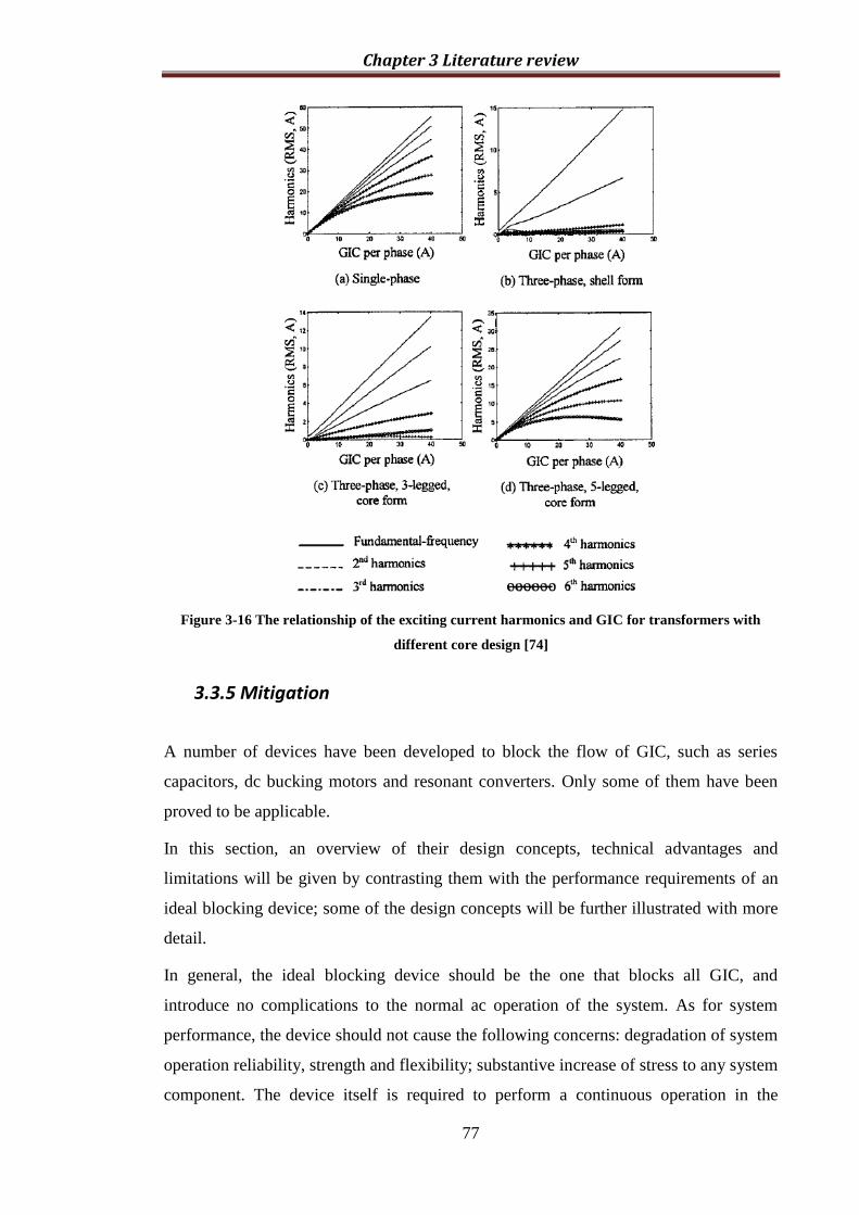
Chapter 3 Literature review
77
Figure 3-16 The relationship of the exciting current harmonics and GIC for transformers with
different core design [74]
3.3.5 Mitigation
A number of devices have been developed to block the flow of GIC, such as series
capacitors, dc bucking motors and resonant converters. Only some of them have been
proved to be applicable.
In this section, an overview of their design concepts, technical advantages and
limitations will be given by contrasting them with the performance requirements of an
ideal blocking device; some of the design concepts will be further illustrated with more
detail.
In general, the ideal blocking device should be the one that blocks all GIC, and
introduce no complications to the normal ac operation of the system. As for system
performance, the device should not cause the following concerns: degradation of system
operation reliability, strength and flexibility; substantive increase of stress to any system
component. The device itself is required to perform a continuous operation in the

Chapter 3 Literature review
78
system and should be reliable during the following conditions: normal and abnormal
steady-state conditions; transient overvoltage contingencies and system faults [75].
There are two types of design concept: passive and active. Passive devices were
designed to block or restrain the flow of GIC current by using resistors or capacitors.
For active devices, they were designed to counteract the GIC current by using an
adjustable current source which can generate a reverse dc current or a reverse
magnetomotive force.
One of the common passive devices is the transmission line series capacitor which can
effectively block the flow of GIC in a specific transmission line. However, the frequent
application of autotransformers complicates the situation, because this type of
transformer allows the GIC to have different flow through the series and common
windings. Hence, the transmission line series capacitor will block the GIC at one
voltage level but will still allow the GIC to flow unimpeded through the other side.
Bearing such a concern in mind, the idea of blocking the GIC current at the transformer
neutral would be more attractive [76]. Passively, this could be achieved by attaching
either resistor or capacitor to the transformer neutral. Actively, this might be achieved
by connecting a separately excited dc motor between the transformer neutral and ground
to inject a reverse dc current.
Apart from blocking the GIC outside the transformer, a method to place an auxiliary
winding on the transformer closed-delta winding has also been proposed. The auxiliary
winding is connected to a current source which can be controlled to cancel the
magnetomotive force generated by the GIC flowing through the high-voltage windings
[77].
The above design concepts should be thoroughly justified by the performance
requirements. Meanwhile, they should be cost-efficient. Table 3-7 is a list of technical
advantages and limitations by contrasting all the design concepts with the performance
and cost requirements.

Chapter 3 Literature review
79
Table 3-7 Advantages and limitations of mitigation devices
Advantages Limitations
Transmission line
series capacitors
[78]
Standard product
and mature
technology
Expensive and difficult to achieve system-
wide application;
May increase system susceptibility to sub-
synchronous resonance;
Adjustable current
sources [78] [79]
Least intervention
to system
grounding
Difficult to achieve total elimination of GIC;
Low efficiency: the dc current generate from
the current supply could be more than ten
times larger than the compensation current;
Capability to withstand system transients is
questionable;
Require precise measurement of GIC
direction and magnitude;
Neutral series
grounding
resistance [80]
Stable and reliable
passive device;
weakly dependent
on the network
configuration;
Only compensate part of the GIC current;
Calculation of appropriate resistance value
requires consideration of geological
structures, soil characteristics and
interaction with pipeline networks, which
also vary with transformer locations;
When the resistance value is big, it will
affect the protection settings;
Neutral series
grounding
capacitor [76, 81,
82]
Completely block
out all the GIC;
Standard product
and mature
technology;
It may hinder the ability of relay systems to
detect and discriminate fault currents;
Careful design of the bypass systems is
needed to achieve insulation coordination
and tolerate worst fault current;
May lead to ferroresonance condition;
Unlike neutral blocking schemes that install blocking devices between transformer
neutral and the ground, the one proposed in [77] suggests mitigating the GIC inside the
transformer. The idea is suitable for those transformers already equipped with a closed-
delta winding, as present on generator step-up transformers. This closed-delta winding
allows the use of a very moderately rated auxiliary winding and controlled current
source. The diagram shown in Figure 3-17 indicates the potential location of the
auxiliary winding.

Chapter 3 Literature review
80
Figure 3-17 GIC mitigation scheme inside power transformer [77]
One study was centred on a step-up transformer rated 525/22.8 kV, YNd, banked from
three single-phase units each rated above 300 MVA. The high voltage and auxiliary
windings have about 1000 and 100 turns respectively. In order to compensate the GIC
which is averaging 10 A in the neutral (over ten minutes), the auxiliary winding needs a
current rating of approximate 30 A to achieve an MMF balance in the core.
The location of the auxiliary winding interior to a delta winding has been evaluated in
[57]. It was found that the induced voltage is greater if the auxiliary winding is moved
up from its optimal position, and less if the auxiliary winding is moved towards the
geometric centre of the transformer.
To apply such a scheme, the capability of the auxiliary winding and the controlled
source used to compensate for GIC need to survive from fault, lighting, switching and
other transient conditions; however if they can succeed or not is still under investigation.
3.4 Discussion and summary
A brief description of switching transient and GIC phenomena in power systems is
given in this chapter. This is followed by a review of the historical research experience
including the waveform analysis, system parameter analysis and transformer saturation
analysis.
A literature review of transformer saturation is organised into two categories, which
result from operational transient and natural transient events, respectively.
As for the switching transients, energisation and de-energisation are represented by the
circuit breaker switching on and off. During these operations, the system network would
have transient states and the transformer could be saturated due to the sudden change
between two steady-state situations. Various investigation methods were used in this

Chapter 3 Literature review
81
field, such as simulations, field tests and validations. More importantly, if the
simulation model was verified by the field test results sensitivity studies were usually
conducted on the key parameters, to identify the worst scenario and so on.
On the other hand, in the field of GIC, researchers from two main fields (i.e. geology
and electrical power engineering) are involved. In this literature review, the electrical
power engineering perspective is mainly provided. The GIC events appeared in the
power system following the solar wind cycle which is normally about 11 years per cycle,
and it could bring operational issues and equipment issues. Various investigations were
conducted and they were mainly associated with power system operation, i.e. reactive
power consumption, voltage drop and protection mal-functions.
A transformer model was used as a tool to facilitate the system side of investigations,
and the transformers were normally modelled with some simply and rather crude
representations.
This research project focuses much more on the transformer itself. How to accurately
model the transformer structure, core and winding, and the transformer’s magnetising
current under ferroresonance and GIC are the main areas of focus for research.
This is particularly important since we know that all the issues in the power system side
related to transformer core saturation, are associated with the behaviour of the
transformer itself. As far as the simulation is concerned, once the transformer is
saturated, taking GIC as an example, how much reactive power is absorbed, how the
voltage drop is formulated and the consequences of affecting the stability of system, is
controlled largely by the accuracy of the transformer model.
In the following chapters, the research work on modelling transformer behaviours under
core saturation problems is described. Two types of models are developed to facilitate
the understanding and interpretation of the GIC and ferroresonance phenomena.

Chapter 4 Steady state magnetic circuit modelling for transformers
82
Chapter 4 Steady state magnetic
circuit modelling for transformers
From Chapter 3, it is known that transformer core modelling methods are essential for
the investigation to be carried out. The accuracy of the transformer model will mainly
determine the validities of the following study results. In this chapter, the work focuses
on transformer core modelling; using the mathematical method to represent the flux
distribution in different transformer core structures. The objects under study are three-
phase three-limb transformers and five-limb three-phase transformers.
Figure 4-1 shows the logic for the whole chapter.
Transformer model
Simple three-limb transformer core
model
Three-limb with return path
transformer core model
Five-limb transformer core
model
Validation by transformer open circuit test data
Comparison of structure effect on
flux distribution and magnetizing
current
Comparison of ratio of side yoke
and main yoke area effect on flux
distribution and magnetizing current
Use an artificial five-limb transformer core parameters
Use a real five-limb transformer core
parameters
Matched with the open-circuit test
data, ready to be used for GIC calculation
Comparison of different working
point effect on flux distribution and
magnetizing current
Build of a three-limb transformer core
model
Build of a three-limb transformer core
model
Validation by transformer open circuit test data
Balanced situation
Unbalanced situation
Validation by transformer open circuit test data
Comparison of ratio of side yoke
and main yoke area effect on flux
distribution and magnetizing current
(See in Appendix)
Figure 4-1 Flow chart of chapter 4’s work

Chapter 4 Steady state magnetic circuit modelling for transformers
83
4.1 Methodology of transformer core modelling
4.1.1 Three-limb transformer core model
4.1.1.1 Simplified three-limb transformer core model
In order to simplify the analysis, there are some assumptions made as follows: the
leakage flux is ignored; the main flux is uniformly distributed along the cross-section of
core; the influence of hysteresis, eddy current and core saturation are neglected; the core
joints are not considered; the three phases flux, ФA, ФB and ФC are sinusoidal and the
120˚ phase relationship to each other.
The instantaneous values of the flux at phase A, B and C are given by:
tmA cos,
)120cos( tmB ,
)240cos( tmC , where Фm is the
flux peak value in the main-limb of core.
The equivalent magnetic circuit of a three-limb transformer is shown in Figure 4-2. In
the figure, R is the reluctance, F is the magneto-motive force (MMF) and Ф is the
magnetic flux.
Figure 4-2 Equivalent magnetic circuit of three-phase three-limb transformer
In an ideal situation three-phase symmetrical fluxes give:
0 (4.1)A B C

Chapter 4 Steady state magnetic circuit modelling for transformers
84
Due to the structure of the three-limb transformer, the flux in the yoke area is equal to
that in the side limb. Since the fluxes applied at the limbs (ФA, ФB and ФC) are
sinusoidal, the fluxes at the yoke of the three-limb transformer are also sinusoidal.
4.1.1.2 Improved three-limb transformer core model
From the last section, the calculation of the three-limb transformer is quite
straightforward. However, this kind of model cannot be used for the calculation of a
saturation situation, because in this model there is no return path considered for the
saturated flux to escape. Therefore, an improved three-limb transformer core model is
presented here.
If the transformer works under a saturation situation, the fluxes, or at least some of them,
would leak out from the transformer core structure, and go through oil, the transformer
tank wall and other components.
In order to simulate the leaked flux, there are two return paths created in the model.
Figure 4-3 shows the improved transformer core model, in which the blue part
represents the transformer core and the green part represents the transformer tank and
oil gaps.
Figure 4-3 Three-limb transformer model with return path
It can be seen from the above figure, that the fluxes are not only going through the
transformer core structure, but also through the transformer tank. Figure 4-4 shows the
equivalent magnetic circuit of the three-phase three-limb transformer with return path.

Chapter 4 Steady state magnetic circuit modelling for transformers
85
Figure 4-4 Equivalent magnetic circuit of three-phase three-limb transformer with return path
For the circuit shown in Figure 4-4, four meshes are defined. Фlt, ФAB, ФBC and Фrt are
assigned to four meshes respectively with the flow direction being mirror symmetric of
the centre.
Kirchhoff Voltage Law (KVL) for magnetic field is applied at each mesh, one at a time,
employing the fact that in the direction of flux Ф the MMF drop across the reluctance is
ФR. The MMF drop across the reluctance is taken in the direction of the mesh flux. The
total MMF drops are set equal to the MMF rise across the MMF source. For example,
the MMF drop across Rlt is ФltRlt while across ROA is (Фlt – ФAB)∙ROA. The derivation of
the formula is presented as follows:
Since the mesh fluxes are given by Фlt, ФAB, ФBC and Фrt a set of four mesh-flux
equations can be written as:
lt ( ) (4.2)lt OA AB OA AR R R F
(2 ) (4.3)lt OA AB AB OA OB BC OB A BR R R R R F F
(2 ) (4.4)AB OB BC BC OB OC rt OC B CR R R R R F F
( ) (4.5)BC OC rt rt OC CR R R F
ФA
ФB
ФC
Фlt
ФAB
ФBC
Фrt
RAB
RAB RBC
RBC
FA FB FC
ROA ROB ROC
RLt RRt

Chapter 4 Steady state magnetic circuit modelling for transformers
86
Kirchhoff Current Law (KCL) for magnetic field is applied for the fluxes at the T-joint
of the circuit to derive, the following equations:
(4.6)lt A AB
(4.7)B AB BC
(4.8)rt C BC
From (4.6) to (4.8) under (4.1) condition, we can obtain:
(4.9)lt rt
Knowing lt rtR R due to the structure of the transformer core, and (4.9) indicates that
the flux flowing in the two side yokes is identical.
Based on (4.9), equations (4.2) to (4.5) are added up together, so the solution can be re-
written as:
2 2 0 (4.10)lt lt AB AB BC BC rt rtR R R R
This equation can be used as the Newton-Raphson condition for the calculation and the
calculation method will be presented in the following sections.
By using (4.6) and (4.8) to replace ФAB, and ФBC, (4.10) following (4.11) for calculating
the flux leaked to the tank can be obtained.
2 2(4.11)
2 2
C BC A ABlt
lt AB BC rt
R R
R R R R
Apply Фlt in (4.10) to (4.7), (4.8) and (4.9); we can obtain the equation for calculating
the flux at the main yoke of the core.
(2 )(4.12)
2 2
B BC rt C rt A ltAB
AB BC lt rt
R R R R
R R R R
Equation (4.11) and (4.12) give the basic equations to define the flux distribution in the
tank and the main yoke of the three-limb transformer.

Chapter 4 Steady state magnetic circuit modelling for transformers
87
The above equations are found to be in the form of reluctance and can be further
expanded using reluctancel
RA
. The expression of ltR , rtR , ABR , BCR can be
rewritten as follows:
2 2; ; ; (4.13)l t l t m m
lt rt AB BC
lt t rt t AB l BC l
L L L L L LR R R R
A A A A
From (4.13), (4.11) and (4.12) can be rewritten as follows:
2 cos( 240 ) cos( )
(4.14)2 2 2 2
om m
BC l AB llt m
l t m m l t
lt t AB l BC l rt t
L Lt t
A A
L L L L L L
A A A A
( )
2 2 2 2cos( 120 )( ) cos( 120 ) cos( )
(4.15)2 2 2 2
o om l t l t l t
BC l rt t rt t lt tAB m
l t m m l t
lt t AB l BC l rt t
L L L L L L Lt t t
A A A A
L L L L L L
A A A A
When (4.14) and (4.15) are obtained, all the flux distribution inside the transformer can
be easily calculated, which means the instantaneous value of the flux at all parts can be
obtained.
From these equations, it seems that the structure parameters of the transformer and the
materials' characteristics are dominating the flux distribution. For the structure, there is
the area of the main limb, yoke and the tank thickness and the length of the yoke, the
length between the core and tank and main limb; for the materials’ characteristics, there
is the varying permeability of the core material and the tank material.
4.1.2 Five-limb transformer core model
For the five-limb transformer core, the equivalent magnetic circuit is shown in Figure
4-5. As for Figure 4-4, R is the reluctance, F is the magneto-motive force (MMF) and Ф
is the magnetic flux in the figure.

Chapter 4 Steady state magnetic circuit modelling for transformers
88
Figure 4-5 Equivalent magnetic circuit of three-phase five-limb transformer
In the five-limb transformer, there is the low-reluctance return path for the unbalanced
flux to pass through easily. There is no need to build up the extra limb to model the
leaked out flux. The circuit shown in Figure 4-5 is almost the same as the improved
three-limb transformer; however, the difference is that there are two different types of
materials characteristics used in the three-limb transformer model. One of the material
characteristics is the core steel characteristic; and the other one is the transformer tank
material characteristic; in the five-limb transformer, it would be much easier, due to the
fact that all the materials are core steel.
Equation (4.16) is the final equation for the Newton-Raphson condition:
2 2 0 (4.16)ls ls AB AB BC BC rs rsR R R R
The flux can be calculated by using the same method as the previous section; the
equations are shown below, which are (4.17) and (4.18).
2 cos( 240 ) cos( )
(4.17)2 2 2 2
om m
BC l AB llt m
l t m m l t
ls t AB l BC l rs t
L Lt t
A A
L L L L L L
A A A A
( )
2 2 2 2cos( 120 )( ) cos( 120 ) cos( )
(4.18)2 2 2 2
o om l t l t l t
BC l rs t rs t ls tAB m
l t m m l t
ls t AB l BC l rs t
L L L L L L Lt t t
A A A A
L L L L L L
A A A A
ФA
ФB
ФC
Фls
ФAB
ФBC
Фrs
RAB
RAB RBC
RBC
FA FB FC
ROA ROB ROC
RLS RRS

Chapter 4 Steady state magnetic circuit modelling for transformers
89
4.1.3 Magnetising current calculation
The magnetising current of a transformer is provided by the manufacturer which is
shown in the certification test report of the particular transformer. As we know, the
magnetising current shown in the open circuit test report includes two parts of the
current, which are the current passing through the core resistance and the current
passing through the core inductance.
The open circuit test gives Rc and Xc which are core resistance and core inductance. This
test is performed by applying the rated voltage (Vs) to the low voltage side while leaving
the high voltage side open circuit. Either side may be used, but the voltage is normally
applied to the low voltage side to reduce the requirement for high voltage test
equipment. Assuming that the shunt impedance, which is the core impedance (Rc and
Xc), is much larger than the series impedance which is primary winding impedance (R1
and X1), the equivalent circuit model can be reduced to Figure 4-6.
Figure 4-6 Equivalent circuits with open circuit test
The values of Ir and Im can be calculated using the following formulas (4.19) and (4.20)
from the voltage (Voc), current (Ioc) and power (Poc) measured in the open circuit test.
2 2
m
/ 3 (4.19)
(4.20)
r oc oc
oc r
I P V
I I I
In addition, the open circuit test is normally carried out at the delta winding which is
normally for the lower voltage level in a transmission power transformer. So all the
magnetising currents measured are line currents.
Ir Im

Chapter 4 Steady state magnetic circuit modelling for transformers
90
4.1.4 Flux density calculation
From the analysis above, it is known that for a three-phase three-limb transformer under
balanced conditions, the computation of flux at the yoke is straightforward. However,
for the improved three-phase three-limb and three-phase five-limb transformer core
model with the non-linearity of core material being considered, the derived flux
formulas show that the magnetic flux calculation are complex. The flux distribution is
dependent on the permeability of the materials and the cross-sectional areas and the
length of the different parts of the transformer. MATLAB simulation will be involved to
calculate the flux density at any part of the three-phase three-limb and five-limb
transformer core structure.
Calculating the instantaneous flux density at any part of the three-phase three-limb and
five-limb transformer core structure is based on the equation BA
. Since the
permeability of the core varies with the flux density, the magnetic material is divided
into sections; it is assumed that each section has a uniform flux density.
If the MMF is set as F R Hl , (4.10) and (4.16) would become:
2 2 0 (4.21)
2 2 0 (4.22)
lt lt AB m BC m rt rt
ls ls AB m BC m rs rs
H l H l H l H l
H l H l H l H l
Significant work has been carried out with the intention to formulate a magnetisation
curve (B-H) representation that is simple and accurate, in order to simplify the
numerical modelling of the transformers. The non-linearity B-H curve can be
represented by a polynomial, which is used to fit the magnetisation characteristic to
provide more flexibility calculations. The magnetisation characteristic can be modelled
by a two-term polynomial relationship between the magnetic field intensity H and the
magnetic field density B:
(4.23)nH aB bB

Chapter 4 Steady state magnetic circuit modelling for transformers
91
The software called ORIGIN is used to process an array of data and fit it using the
formula as above. Due to the different designs of transformers produced during the
period 1950-today and by different manufacturers, the transformers being picked up in
this investigation used different types of core steels; the following data is supplied by
Japan Nippon Steel Corporation, Japan:
-5 2720.34 (4.55 x 10 ) (4.24)H B B
The curve fitting result is shown in Figure 4-7. Equation (4.24) presents the twenty-
seventh order polynomial representation of the magnetisation curve. This equation is
incorporated into MATLAB script (all the code and data are included in the appendix)
in order to find H that corresponds to the calculated B values. This analytical
representation enables the incorporation of the non-linear effects of the core into the
proposed analytical transformer core model.
Figure 4-7 Curve fitting result for Japan Nippon steel corporation materials
In addition, we need to understand that Figure 4-7 shows the core steel materials
characteristics. The transformer core structure is not only made of core steel material,
but also has air gaps between each lamination in the joint area. Therefore, as we know
the transformer core characteristic would be changed due to the air gap in the magnetic
circuit. Therefore the fitted curve needs to be further refined.
By using MATLAB, the flux density at each part of the transformer core is calculated.
The MATLAB programme is based on the flow chart that is shown in Figure 4-8. First,

Chapter 4 Steady state magnetic circuit modelling for transformers
92
input the basic parameters of the transformer structure; second, at each time step assume
an initial value for Ф1 and use (4.21) or (4.22) to control it by using the Newton-
Raphson iterative method. The accuracy can be controlled by the tolerance set for the
error and the fine time step.
START
Input transformer design data
The start time as 0
Calculate ФA, ФB,ФC in each time step
Initialisation Фlt value as the maximum flux value in the core
Calculate all the other part Ф value
Check the condition true/false
False
T=0.04s
True
Decrease Фlt value
END
True
False
Calculate the corresponding H value by using Non-linear B-H Curve
Increase time step
Initialize each parameter in the program
Figure 4-8 Flow Chart of the MATLAB programme

Chapter 4 Steady state magnetic circuit modelling for transformers
93
4.1.5 Curve fitting
There are two methods to model the transformer nonlinearity characteristics. One is to
use the three points of the transformer open circuit test data, and the other one is to use
the core steel material’s characteristics.
Using the three points to fit the transformer core nonlinear characteristic curve, the
accuracy cannot be guaranteed, since the data points are too few to accurately represent
the nonlinearity curve. However, the advantage of this method is that the core loss has
been considered and also the nonlinearity curve shows the characteristics of the
transformer structure.
Using the core steel material’s data to fit the core transformer nonlinearity characteristic
curve, the accuracy is far better than the previous method, because the data sheet of the
steel normally provides at least 10 points. However the disadvantage of this method is
that the core loss cannot be considered, and the transformer structure influence within
the joint area is not included.
The MATLAB mathematical model has not considered the loss of the core material; all
the investigations in terms of curve fitting use the core steel material’s data to fit the
curve.
Once the curve has been fitted, the verification will be carried out by using the
transformer open circuit test data. As mentioned before, since the air gap is included in
the magnetic circuit, the characteristics may change. Therefore further modification of
the nonlinearity curve needs to be done before using the transformer model to carry out
further studies.
In summary, the best way to do the curve fitting in order to simulate the transformer
non-linearity is to combine both of the core material’s characteristics with the
transformer open test data. Use the core material’s characteristics to fit the curve first,
and then use the transformer open circuit test data to modify the fitted curve.

Chapter 4 Steady state magnetic circuit modelling for transformers
94
4.2 Case 1: Magnetising current investigation
In the last section, there are two transformer models for the three-phase three-limb
transformer and one model for the five-limb transformer. All the models will be used to
investigate the influence of the transformer structure on the magnetising current.
4.2.1 132/33 kV, 90 MVA three-limb transformer
The simulation was carried out using one of the transformers in the distribution
substations in Manchester, UK as part of the case study. The transformer is a 132/33 kV,
90 MVA, three-limb core type transformer. The basic information needed for the
mathematical magnetic circuit model is the basic dimensions of the transformer core
structure. The dimensions of the transformer are shown in Table 4-1, which include the
core dimensions, the max flux density under rated voltage, the winding connection and
turn number, the tank dimension and the air gap between the transformer core and tank.
It is assumed that the leaking flux goes directly to the top/bottom of the tank and
follows this path through the side of tank and finally returns to the core again. Based on
this assumption, the maximum return path length can be calculated by summarising the
tank height and length, two air gaps between the top/bottom of the core and the
top/bottom of the tank length and two parts of the top/bottom tank length. The
maximum return path area can be calculated by summarising the lateral areas of the tank.
Table 4-1 132/33 kV dimensions data
No. Parameters
1 Main limb effective length /m 2.63
2 Main yoke effective length /m 1.48
3 Main limb cross-section area /m2 0.306369
4 Main yoke cross-section area /m2 0.306369
5 Max flux density under rated voltage /T 1.523
6 Primary winding turn number 697
7 Secondary winding turn number 318
8 Connection Y/ delta
9 Tank length /m 4.8
10 Tank width /m 2
11 Tank height /m 3.7
12 Tank thickness /m 0.1
13 Max return path length /m 6.1
14 Max return path area /m2 5.032

Chapter 4 Steady state magnetic circuit modelling for transformers
95
The three-limb transformer is produced by Alstom in Stafford, UK, and the core steel
material (23M3) characteristics for building up the transformer and the mild steel
material characteristics for building up the tank are shown in Figure 4-9. The blue line
shows the transformer core material characteristics and the red line shows the tank mild
steel material characteristics.
Figure 4-9 Material non-linear characteristics
It can be seen from Figure 4-9, that the materials’ characteristics are quite different. The
transformer core steel material is easier to saturate and the knee point is higher that of
the tank mild steel. Therefore, if the transformer core is working, balanced and lower
than the knee area, all the flux should be passing through the core, negligible flux could
be in the tank.
There are two models proposed for three-limb transformers; then the simulation would
be carried out for comparison purposes between the calculated magnetising currents of
those two models and the test report data.
Normally the transformer manufacturer only provides the open circuit test data for the
supplying voltages at 90%, 100% and 110% of the rated level. Therefore, the
simulations are carried out by following the open circuit test procedure. Figure 4-10 (a),
(b) and (c) shows that when varying the supplying voltage at 90%, 100% and 110%, the
magnetising currents of three phases are calculated by the two different models.

Chapter 4 Steady state magnetic circuit modelling for transformers
96
(a)
(b)
(c)
Figure 4-10 Three-phase magnetising currents of different supplied voltage level
-2
-1.5
-1
-0.5
0
0.5
1
1.5
2
-40
-30
-20
-10
0
10
20
30
40
0 0.01 0.02 0.03 0.04
Cu
rre
nt(
A)
Vo
ltag
e(k
V)
Time(s)
Magnetising currents in a 3-Limb transformer under 90% rated voltage
Vab Vbc Vca Iab Ibc Ica Iab(Return Path) Ibc(Return Path) Ica(Return Path)
-2
-1.5
-1
-0.5
0
0.5
1
1.5
2
-40
-30
-20
-10
0
10
20
30
40
0 0.01 0.02 0.03 0.04C
urr
en
t(A
)
Vo
ltag
e(k
V)
Time(s)
Magnetising currents in a 3-Limb transformer under 100% rated voltage
Vab Vbc Vca Iab Ibc Ica Iab(Return Path) Ibc(Return Path) Ica(Return Path)
-2
-1.5
-1
-0.5
0
0.5
1
1.5
2
-40
-30
-20
-10
0
10
20
30
40
0 0.01 0.02 0.03 0.04
Cu
rre
nt(
A)
Vo
ltag
e(k
V)
Time(s)
Magnetising currents in a 3-Limb transformer under 110% rated voltage
Vab Vbc Vca Iab Ibc Ica Iab(Return Path) Ibc(Return Path) Ica(Return Path)

Chapter 4 Steady state magnetic circuit modelling for transformers
97
In this figure, the round dot lines represent the supplied voltage; the solid lines represent
the simulation results of the simple three-phase three-limb transformer model and the
dashed lines represent the simulation by the improved three-phase three-limb
transformer results. It can be seen from Figure 4-10 (a), (b) and (c), when the supplied
voltage is 90% and 100% of the rated voltage, the magnetising currents are of the
sinusoidal waveform; when the supplied voltage reaches 110% of the rated voltage, the
magnetising currents are distorted by the harmonics. And the magnitude of the blue
phase of the magnetising current is higher than the other two phases, and this matches
the fundamental theory mentioned earlier in Chapter 2. However, the phase shift
between two adjacent phases does follow the fundamental theory of 120˚ apart; the red
and yellow phases are quite close to each other and away from the blue phase.
There are two different methods that are used to calculate the RMS value of the
magnetising currents. Sometimes they just measure the peak value of the waveform and
then divide it by root two, sometimes they calculate the RMS by using the formula
2
0
1T
RMSI i dtT
, T is the period of the fundamental harmonic, i is the magnitude of
the current.
Table 4-2 shows the comparison between the simulation results with the test results by
using the two different methods to calculate RMS (root mean square) value of the
magnetising currents.
Table 4-2 Comparison the RMS magnetising currents in field test data and simulation results
Supplied voltage (% of rated) Iab(A) Ibc(A) Ica(A)
Test Report
90% 0.55 0.51 0.71
100% 0.69 0.68 0.88
110% 1.01 1.01 1.17
3-Limb Model
90% 0.56 0.56 0.75
100% 0.64 0.64 0.85
110% 0.95 0.95 1.26
3-Limb
(Return Path) Model
90% 0.56 0.56 0.73
100% 0.63 0.63 0.82
110% 0.85 0.85 1.07
It can be seen in Table 4-2 that the RMS value of the phase Iab and Ibc is lower than the
Ica. The simulation results for 90% and 100% voltage supply are very similar to those of
the test report. However, the simulation results for currents do not match well with the
test report under the 110% rated voltage supplied. This is because the magnetising

Chapter 4 Steady state magnetic circuit modelling for transformers
98
current is distorted during the 110% rated voltage supplied, due to the transformer core
saturation. The test report data is calculated by using the peak value divide root two
method. The simulation results are calculated by using the formula2
0
1T
RMSI i dtT
,
and then the only fundamental frequency is taken into account. This is the reason why
the results of the test data are slightly higher than the simulation results.
Table 4-3 shows the phase angles of the magnetising currents by varying the magnitude
of supplied voltage. Ica is at the 150˚ as the reference. It is easily seen that those three-
phase currents do follow the rule of the 120˚ apart. The red and yellow phases are 12˚
away from the baseline; the phase shift can be influenced by the supplied voltage in the
simple three-limb model.
Table 4-3 Phase angle calculated for magnetising currents for three phases
Supplied voltage (% of rated) Iab(angle) Ibc(angle) Ica(angle)
3-Limb
90% 18 -78 150
100% 18 -78 150
110% 18 -78 150
3-Limb
(Return Path)
90% 19 -79 150
100% 19 -79 150
110% 21 -81 150
4.2.2 400/275/13 kV, 1000 MVA five-limb transformer
In this section, some of the five-limb transformer design data and the open circuit test
data are used to examine the five-limb core model.
Table 4-4 shows the design data of the 400/275/13 kV five-limb transmission
transformer. The core dimensions are used to calculate the flux distribution and the field
intensity as well; once the field intensity is obtained, the magnetising currents can be
calculated by using the winding turn number and the voltage level. Both the line current
and phase current can be calculated as well.

Chapter 4 Steady state magnetic circuit modelling for transformers
99
Table 4-4 400/275/13 kV five-limb transformer data
No. Parameters
1 Main limb effective length /m 2.76
2 Main yoke effective length /m 2.57
3 Side yoke effective length /m 1.6475
4 Main limb cross-section area /m2 0.6438
5 Main yoke cross-section area /m2 0.3884
6 Side yoke cross-section area /m2 0.3884
7 Max flux density under rated voltage /T 1.694
8 Primary winding turn number 960
9 Tertiary winding turn number 54
10 Connection Y-Y-Δ
In Figure 4-11, the blue line represents the permeability change by varying the magnetic
field intensity, and the red line represents the materials’ B-H curve. It is easy to see that
when B-H curve reaches the knee area, the permeability starts to reduce; and when B
becomes flat in the deep saturation region, the permeability is reduced near to the level
of µ0(4π×10-7
), which is 2.3×10⁻⁵
.
Figure 4-11 Flux density and permeability of the µ0µr by varying magnetic field intensity
Once all the information of the transformer is input into the MATLAB programme, the
Newton-Raphson Method would minimize the error for the solution and solve the
problem within a given tolerance.
Figure 4-12 shows the three-phase magnetising current waveforms and the supplied
voltage waveform. The dotted lines represent the supplied voltage and the solid lines
0
0.01
0.02
0.03
0.04
0.05
0.06
0
0.2
0.4
0.6
0.8
1
1.2
1.4
1.6
1.8
2
0 20 40 60 80 100 120
Pe
rme
abili
ty µ
0µr
Ma
gne
tic
Fie
ld D
en
sity
(T)
Magnetic Field Intensity (H/m)B Mu

Chapter 4 Steady state magnetic circuit modelling for transformers
100
represent the magnetising current. The voltage is represented using the left Y-axis, and
magnetising current uses the left Y-axis. The red, yellow and blue lines represent phase
A, B and C respectively.
(a)
(b)
-10
-8
-6
-4
-2
0
2
4
6
8
10
-250
-200
-150
-100
-50
0
50
100
150
200
250
0 0.01 0.02 0.03 0.04
Cu
rre
nt
(A)
Vo
ltag
e (
kV)
Time(s)
Magnetising currents in a 5-Limb transformer under 90% rated voltage
-20
-15
-10
-5
0
5
10
15
20
-300
-200
-100
0
100
200
300
0 0.01 0.02 0.03 0.04
Cu
rre
nt
(A)
Vo
ltag
e (
kV)
Time(s)
Magnetising currents in a 5-Limb transformer under 100% rated voltage

Chapter 4 Steady state magnetic circuit modelling for transformers
101
(c)
Figure 4-12 Three-phase five-limb transformer core magnetising currents of different supplied
voltage level
It can be seen from Figure 4-12, that when the supplied voltage is 90% of the rated
voltage the magnetising current can still follow the sinusoidal waveform; when the
supplied voltage is increased to 100% and 110%, the magnetising currents are distorted
and the magnitudes increase significantly. The phase shifts between each pair of
adjacent phases would also be changed; this is shown in Table 4-5. It is the same reason
as the three-limb transformer; it is due to the part of the transformer core saturated and
the flux re-distribution in the whole magnetic circuit.
Table 4-5 Phase angle for each magnetising current in each phase
Supplied voltage
(% of rated) Iab(Angle) Ibc(Angle) Ica(Angle)
90% 24 -84 150
100% 26 -86 150
110% 29 -89 150
Table 4-6 shows the comparison between open circuit test results with the simulation
results of magnetising currents in RMS value.
Table 4-6 Comparison the RMS magnetising current in simulation results and field test data
Supplied voltage
(% of rated) Iab(A) Ibc(A) Ica(A)
Test data
90% 5.25 6.00 7.28
100% 12.30 12.40 14.75
110% 55.2 54.3 56.8
Simulation results
90% 6.62 6.62 7.84
100% 10.58 10.58 11.95
110% 51.36 51.36 52.78
-80
-60
-40
-20
0
20
40
60
80
-300
-200
-100
0
100
200
300
0 0.01 0.02 0.03 0.04
Cu
rre
nt
(A)
Vo
ltag
e (
kV)
Time(s)
Magnetising currents in a 5-Limb transformer under 110% rated voltage

Chapter 4 Steady state magnetic circuit modelling for transformers
102
It can be seen that the simulation results are well matched with the test results for the
five-limb transformer; it has the same trend as the three-limb transformer, which is that
the magnetising currents in the red and yellow phase are lower than that of the blue
phase. However, the unbalanced situation is better than the three-limb transformer. The
unbalanced magnitude ratio of the red phase to blue phase in the three-limb transformer
is around 75%, but in the five-limb transformer it is around 85%.
Comparing the test and simulation data, it can be seen that the test result is larger than
the simulation under 90% supplied voltage, and smaller at 100% and 110%; but the
results are all reasonable.
Table 4-7 shows the phase currents. It can be seen that the magnitude of yellow phase
current is always higher than other two phases, due to the fact that the magnetic circuit
loops for phases are different. The open circuit test data looks like this, because the
transformers do not have a delta winding and the open circuit tests were carried out at
the Y connection side.
Table 4-7 RMS value of phase current
Magnitude Ia(A) Ib(A) Ic(A)
90% 4.02 4.51 4.02
100% 6.37 7.06 6.37
110% 34.54 35.08 34.54
Figure 4-13 shows the sequence component contents of the magnetising currents by
varying the supplied voltage.
Figure 4-13 Current sequence component content of different supplied voltage level
0
10
20
30
40
50
0 100 200 300 400 500 600 700 800 900 1000
Mag
nit
ud
e o
f cu
rre
nt
(A)
Frequency (Hz)
Sequence currents content
Zero(90%) Positive(90%) Negative(90%) Zero(100%) Positive(100%)
Negative(100%) Zero(110%) Positive(110%) Negative(110%)

Chapter 4 Steady state magnetic circuit modelling for transformers
103
It can be seen that the majority of the magnitude is still contributed by the positive
sequence. However, when the voltage supplied is 90% of the rate voltage, the negative
sequence magnetising current has already existed. This means that the negative
sequence component appears because the magnetic circuits of the three-phase are not
balanced.
Figure 4-13 discusses the unbalanced situation of the magnetising current from a three-
phase perspective. Figure 4-14 shows the frequency contents in the line magnetising
currents.
Figure 4-14 Frequency contents of line magnetising currents of different supplied voltage level
It can be seen that when the supplied voltage is increased the harmonics of the
magnetising current are increased, due to transformer nonlinear saturation. The 3rd
harmonic of line current is nearly zero, this is because the delta winding can absorb the
3rd harmonic. Figure 4-15 shows the flux density in the five-limb transformer core by
varying the supplied voltages. There are four groups of flux densities which are at the
yoke between A and B limb (Bab), yoke between B and C limb (Bbc), right side yoke (Brs)
and left side yoke (Bls).
0
10
20
30
40
50
0 100 200 300 400 500 600 700 800 900 1000
Mag
nit
ud
e o
f cu
rre
nt
(A)
Frequency (Hz)
Frequency content of line magnetising currents
Iab(90%) Ibc(90%) Ica(90%) Iab(100%) Ibc(100%)Ica(100%) Iab(110%) Ibc(110%) Ica(110%)

Chapter 4 Steady state magnetic circuit modelling for transformers
104
Figure 4-15 Flux density in 5-limb transformer core
It can be seen that the flux density waveforms are all distorted; the magnitude of the
flux density in the main yoke area do not change much, only the flat top duration of the
waveform with the increase of the supplied voltage. However the magnitudes of the flux
density of the side yoke area are sensitive to the supplied voltages and their magnitudes
have increased from 1 T to 1.5 T for the increase of supplied voltage from 90% to 110%
rated voltage.
Figure 4-16 shows the field intensity in the five-limb transformer core by varying the
supplied voltages. There are four groups of field intensities which are at the yoke
between A and B limb (Bab), the yoke between B and C limb (Bbc), the right side yoke
(Brs) and the left side yoke (Bls).
Figure 4-16 Field intensity in 5-limb transformer core
-2
-1.5
-1
-0.5
0
0.5
1
1.5
2
0 0.01 0.02 0.03 0.04
B (
T)
Time (s)
Flux density in 5-Limb transformer core under 90%,100% and 110% rated voltage
Bls(90%) Bab(90%) Bbc(90%) Brs(90%) Bls(100%) Bab(100%)Bbc(100%) Brs(100%) Bls(110%) Bab(110%) Bbc(110%) Brs(110%)
Bab Bbc
BlsBrs
-100
-75
-50
-25
0
25
50
75
100
0 0.01 0.02 0.03 0.04
H (
A/m
)
Time(s)
Field intensity in 5-Limb transformer core under 90%,100% and 110% rated voltage
Hls(90%) Hab(90%) Hbc(90%) Hrs(90%) Hls(100%) Hab(100%)Hbc(100%) Hrs(100%) Hls(110%) Hab(110%) Hbc(110%) Hrs(110%)
Hab Hbc
HlsHrs

Chapter 4 Steady state magnetic circuit modelling for transformers
105
It can be seen that the field intensity is in an opposite way to the flux density; the field
intensity does not change much in the side yoke area; however the magnitude of field
intensity in the main yoke area is increased gradually with the increase of supplied
voltage.
4.2.3 Comparison of influence between three-limb and five-limb
transformer structure
In the last two sections, the two models of the three-phase three-limb transformer and
the five-limb transformer model have been examined through open circuit test results.
In this section, the core structure influences are discussed and examined by using an
artificial three-phase five-limb transformer which has the same power rating and the
same voltage level as the transformer in section 4.2.1.
Table 4-8 shows the artificial five-limb transformer dimension data based on those in
Table 4-1. Except for the fact that the area is 50% that of the main limb, the main yoke
and the side yoke and the rest of the parameters are the same as those of the three-limb
transformer.
Table 4-8 Artificial five-limb transformer data based on 132/33 kV dimensions data
No. Parameters
1 Main limb effective length /m 2.63
2 Main yoke effective length /m 1.48
3 Side yoke effective length /m 1.055
4 Main limb cross-section area /m2 0.306369
5 Main yoke cross-section area /m2 0.153184
6 Side yoke cross-section area /m2 0.153184
7 Max flux density under rated voltage /T 1.523
8 Primary winding turn number 697
9 Secondary winding turn number 318
10 Connection Y-Δ
The comparison between these two core structures is carried out with three cases when
the transformers are working at the linear region, the rated voltage and the non-linear
region.

Chapter 4 Steady state magnetic circuit modelling for transformers
106
4.2.3.1 Comparison in linear region
The comparison is carried out between the magnetising currents of three-limb and five-
limb transformers.
Figure 4-17 shows the comparison between the three-limb and five-limb transformer in
terms of magnetising current when the supplied voltage is at the RMS value. The
supplied voltage is 70% of the rated voltage. The dotted line represents the blue phase
of the three-phase supplied voltage; the solid lines represent the blue phase magnetising
currents of the two different core structures. It can be seen that the magnetising current
nearly follows the pure fundamental sinusoidal waveform for both core structures. The
higher value is for the five-limb core transformer. However the phase angles of the
magnetising currents of the blue phase are the same for three-limb and five-limb core
transformers.
Figure 4-17 Comparison of magnetising currents in three-limb and five-limb transformer
Figure 4-18 shows the sequence component contents of the magnetising currents in the
two different core structures. The positive sequence of the magnetising current in the
five-limb transformer is higher than the three-limb transformer; but the negative
sequence of the magnetising current is lower. This proves that the magnetising current
in a five-limb transformer is more balanced than the three-limb transformer.
-1
-0.5
0
0.5
1
-30
-20
-10
0
10
20
30
0 0.01 0.02 0.03 0.04
Cu
rre
nt
(A)
Vo
ltag
e (
kV)
Time(s)
Magnetising currents in a 3&5-Limb transformers (linear region)
Vab Vbc Vca Iab(3-L) Ibc(3-L)
Ica(3-L) Iab(5-L) Ibc(5-L) Ica(5-L)

Chapter 4 Steady state magnetic circuit modelling for transformers
107
Figure 4-18 Comparison of current sequence component contents in three-limb and five-limb core
transformers
Figure 4-19 shows the comparison of the frequency contents of the magnetising currents
in three-limb and five-limb transformers. The same trend can be seen as in the last
figure. The ratio of the Iab (or Ibc) and Ica is 75% in the three-limb transformer and 81%
in the five-limb transformer.
Figure 4-19 Comparison of frequency contents of magnetising currents in three-limb and five-limb
transformers
Figure 4-20 shows the flux density and field intensity of the yoke between the limb
A&B/B&C (a) and the left/right side of tank (b) in the three-limb transformer. The 70%
of the rated voltage convert to a flux density in the main limb of 1.1 T. When the
supplied voltage is only 70% of the rated voltage, all the flux densities in the three-limb
0
0.1
0.2
0.3
0.4
0.5
0.6
0.7
0 100 200 300 400 500 600 700 800 900 1000
Mag
nit
ud
e o
f cu
rre
nt
(A)
Frequency(Hz)
Sequence component contents of magnetising currents (linear region)
Zero(3-L) Positive(3-L) Negative(3-L) Zero(5-L) Positive(5-L) Negative(5-L)
0
0.1
0.2
0.3
0.4
0.5
0.6
0.7
0.8
0 100 200 300 400 500 600 700 800 900 1000
Mag
nit
ud
e o
f cu
rre
nt
(A)
Frequency (Hz)
Frequency contents of line magnetising currents (linear region)
Iab(3-L) Ibc(3-L) Ica(3-L) Iab(5-L) Ibc(5-L) Ica(5-L)
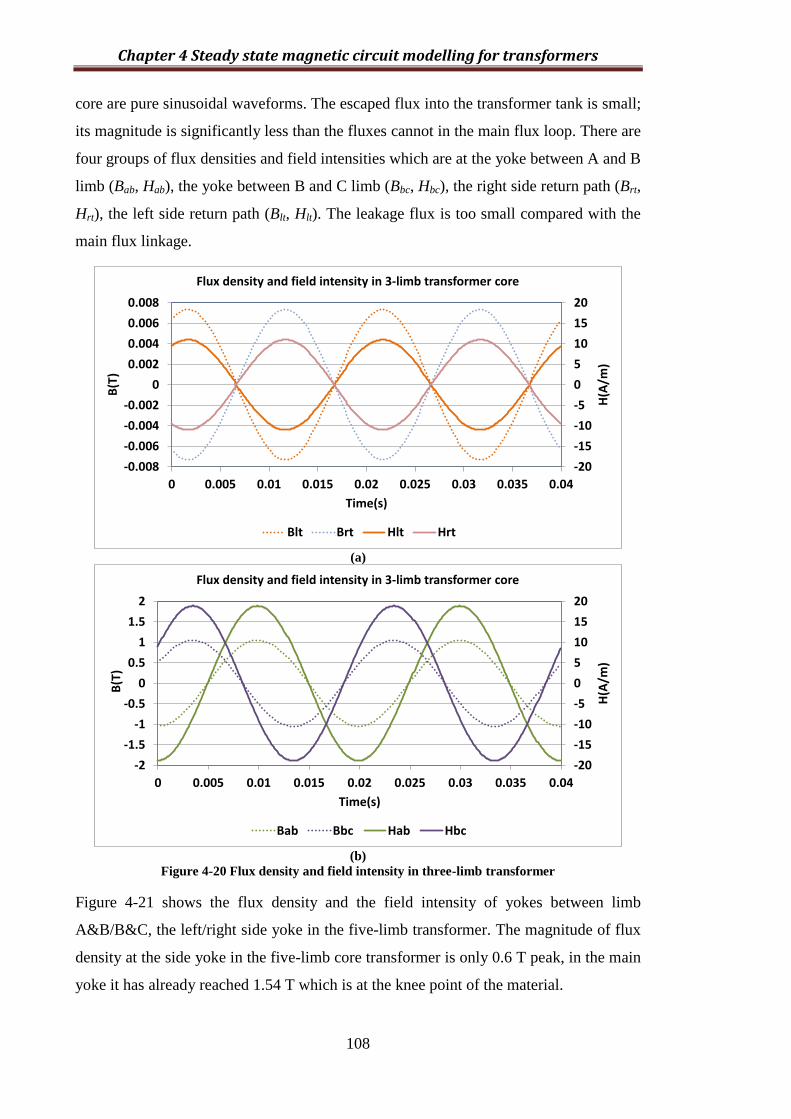
Chapter 4 Steady state magnetic circuit modelling for transformers
108
core are pure sinusoidal waveforms. The escaped flux into the transformer tank is small;
its magnitude is significantly less than the fluxes cannot in the main flux loop. There are
four groups of flux densities and field intensities which are at the yoke between A and B
limb (Bab, Hab), the yoke between B and C limb (Bbc, Hbc), the right side return path (Brt,
Hrt), the left side return path (Blt, Hlt). The leakage flux is too small compared with the
main flux linkage.
(a)
(b)
Figure 4-20 Flux density and field intensity in three-limb transformer
Figure 4-21 shows the flux density and the field intensity of yokes between limb
A&B/B&C, the left/right side yoke in the five-limb transformer. The magnitude of flux
density at the side yoke in the five-limb core transformer is only 0.6 T peak, in the main
yoke it has already reached 1.54 T which is at the knee point of the material.
-20
-15
-10
-5
0
5
10
15
20
-0.008
-0.006
-0.004
-0.002
0
0.002
0.004
0.006
0.008
0 0.005 0.01 0.015 0.02 0.025 0.03 0.035 0.04
H(A
/m)
B(T
)
Time(s)
Flux density and field intensity in 3-limb transformer core
Blt Brt Hlt Hrt
-20
-15
-10
-5
0
5
10
15
20
-2
-1.5
-1
-0.5
0
0.5
1
1.5
2
0 0.005 0.01 0.015 0.02 0.025 0.03 0.035 0.04
H(A
/m)
B(T
)
Time(s)
Flux density and field intensity in 3-limb transformer core
Bab Bbc Hab Hbc

Chapter 4 Steady state magnetic circuit modelling for transformers
109
Figure 4-21 Flux density and field intensity in five-limb transformer
There are four groups of flux densities and field intensities which are at the yoke
between A and B limb (Bab, Hab), the yoke between B and C limb (Bbc, Hbc), the right
side yoke (Brs, Hrs), the left side yoke (Bls, Hls). The leakage flux is too small compared
with the main flux linkage.
4.2.3.2 Comparison in rated voltage
In this section, the comparison is carried out between the magnetising currents, flux
distributions of three-limb and five-limb transformer core and field intensities of three-
limb and five-limb transformer core under the rated voltage.
Figure 4-22 shows that the magnetising currents in two different core transformer
structures under the rated voltage which is represented by the dotted lines Vab, Vbc and
Vca. It can be seen that the magnetising current of the three-limb transformer follows the
sinusoidal waveform which is represented by the solid lines Iab(3-L), Ibc(3-L) and Ica(3-L)
and the magnetising current of five-limb transformer is distorted and the magnitude is
higher than that of the three-limb transformer, as shown in Iab(5-L), Ibc(5-L) and Ica(5-L).

Chapter 4 Steady state magnetic circuit modelling for transformers
110
Figure 4-22 Comparison of magnetising currents in three-limb and five-limb transformers at 100%
rated voltage
Figure 4-23 shows that the sequence component contents of magnetising currents in two
different core structures at 100% rated voltage supplied situation. It is easy to see that
the magnitudes of the fundamental components in the five-limb transformer are higher
than those of the three-limb one. In addition, the negative sequence third harmonic
appears in the five-limb transformer, since a part of the transformer core is saturated.
Figure 4-23 Comparison sequence contents of magnetising currents two different core structures
Figure 4-24 shows the frequency contents of the magnetising currents at 100% rated
voltage. It can be seen that the same trend is shown as Figure 4-23, though the
magnitude of the magnetising current of the fundamental harmonic of the five-limb
-2
-1.5
-1
-0.5
0
0.5
1
1.5
2
-40
-30
-20
-10
0
10
20
30
40
0 0.01 0.02 0.03 0.04
Cu
rre
nt(
A)
Vo
ltag
e (
kV)
Time(s)
Magnetising currents in 3-limb & 5-limb transformers at 100% rated voltage
Vab Vbc Vca Iab(3-L) Ibc(3-L)
Ica(3-L) Iab(5-L) Ibc(5-L) Ica(5-L)
0
0.2
0.4
0.6
0.8
1
1.2
0 100 200 300 400 500 600 700 800 900 1000
Mag
nit
ud
e o
f cu
rre
nt
(A)
Frequency (Hz)
Sequence component contents of magnetising currents (rated voltage)
Zero(3-L) Positive(3-L) Negative(3-L) Zero(5-L) Positive(5-L) Negative(5-L)

Chapter 4 Steady state magnetic circuit modelling for transformers
111
transformer is around 33% higher than that of the three-limb transformer. The third and
fifth harmonic appears in the magnetising current of the five-limb transformer.
Figure 4-24 Comparison frequency contents of line magnetising currents at 100% rated voltage
Figure 4-25 shows the flux density and field intensity in the three-limb core. The flux
density and the field intensity is still a sinusoidal waveform, and the leakage flux is a
hundred times smaller than the flux linkage.
(a)
0
0.2
0.4
0.6
0.8
1
1.2
1.4
0 100 200 300 400 500 600 700 800 900 1000
Mag
nit
ud
e o
f cu
rre
nt
(A)
Frequency (Hz)
Frequency contents of line magnetising currents (rated voltage)
Iab(3-L) Ibc(3-L) Ica(3-L) Iab(5-L) Ibc(5-L) Ica(5-L)
-30
-20
-10
0
10
20
30
-0.015
-0.01
-0.005
0
0.005
0.01
0.015
0 0.01 0.02 0.03 0.04
H(A
/m)
B(T
)
Time(s)
Flux density and field intensity in 3-limb transformer core(100% rated voltage)
Blt Brt Hlt Hrt

Chapter 4 Steady state magnetic circuit modelling for transformers
112
(b)
Figure 4-25 Flux density and field intensity in three-limb transformer at 100% rated voltage
Figure 4-26 shows the flux density and field intensity in the five-limb transformer. It
can be seen that the flux density is seriously distorted. The flux at the main yoke is
saturated and the saturated period is around 1/2 cycle in every cycle. The side yoke is
also distorted due to the main yoke saturation. The field intensity is also distorted; the
third and fifth harmonic appears in both of the main yoke and side yoke.
Figure 4-26 Flux density and field intensity in five-limb transformer at 100% rated voltage
4.2.3.3 Comparison in nonlinear region
In this section, the comparison is carried out between the magnetising currents at the
supplied voltage of 120% rated voltage. The flux distributions and filed intensities of
the three-limb and five-limb core transformers.
-30
-20
-10
0
10
20
30
-1.5
-1
-0.5
0
0.5
1
1.5
0 0.005 0.01 0.015 0.02 0.025 0.03 0.035 0.04
H(A
/m)
B(T
)
Time(s)
Flux density and field intensity in 3-limb transformer core(100% rated voltage)
Bab Bbc Hab Hbc
-100
-50
0
50
100
-2
-1.5
-1
-0.5
0
0.5
1
1.5
2
0 0.005 0.01 0.015 0.02 0.025 0.03 0.035 0.04
H(A
/m)
B(T
)
Time(s)
Flux density and Field Intensity in 5-limb transformer core(100% rated voltage)
Bls Bab Bbc Brs Hls Hab Hbc Hrs

Chapter 4 Steady state magnetic circuit modelling for transformers
113
Figure 4-27 shows the magnetising currents of two different core structures and the
supplied voltage waveforms. The peak magnitude of the magnetising current is almost
ten times the rate of the magnetising current. The five-limb core transformer has a larger
magnetising current than the three-limb one.
Figure 4-27 Comparison of magnetising currents in 3 & 5-limb transformers at non-linear region
Figure 4-28 shows the sequence contents of magnetising currents in two different core
structures at the non-linear region. It can be seen that the harmonics of the positive and
negative sequence components appear. There is no zero sequence content for the
supplied voltages are a pure three-phase ideal balanced voltage source. The 3rd order
harmonic is relatively lower than the other harmonics. The fifth negative harmonic is
higher than the positive one; so is the 11th harmonic.
Figure 4-28 Comparison of current sequence contents in 3&5 limb transformer at nonlinear region
-15
-10
-5
0
5
10
15
-60
-40
-20
0
20
40
60
0 0.01 0.02 0.03 0.04
Cu
rre
nt
(A)
Vo
ltag
e (
kV)
Time(s)
Magnetising currents in 3-limb and 5-limb transformer (nonlinear region)
Vab Vbc Vca Iab(3-L) Ibc(3-L)Ica(3-L) Iab(5-L) Ibc(5-L) Ica(5-L)
0
1
2
3
4
5
6
0 100 200 300 400 500 600 700 800 900 1000
Mag
nit
ud
e o
f C
urr
en
t (A
)
Frequency (Hz)
Sequence component contents of magnetising currents (nonlinear region)
Zero(3-L) Positive(3-L) Negative(3-L) Zero(5-L) Positive(5-L) Negative(5-L)

Chapter 4 Steady state magnetic circuit modelling for transformers
114
Figure 4-29 shows the frequency content in each phase of the magnetising current at the
nonlinear region. It can be seen that the third harmonic is lower than the fifth and
seventh harmonic due to the delta winding connection. Iab and Ibc are always lower than
Ica in the entire frequency scan range.
Figure 4-29 Comparison of frequency contents of three-limb and five-limb transformers
magnetising currents at nonlinear region
Figure 4-30 shows the flux densities and field intensities in the three-limb transformer
core at the nonlinear region. Figure 4-30 (a) shows the flux densities and field
intensities in the transformer tank, and Figure 4-30 (b) shows the flux densities and field
intensities in the yoke. The highest peak magnitude of the flux density can achieve 1.8T,
and the waveform is distorted. The escaped flux is still low which is 0.0315T; that is the
reason why it cannot be seen in the figure. The field intensity is 30 times higher than the
rated situation.
In addition, the waveform is distorted with the third harmonic and fifth harmonic
content.
0
1
2
3
4
5
6
7
0 100 200 300 400 500 600 700 800 900 1000
Mag
ne
itu
de
of
Cu
rre
nt
(A)
Frequency (Hz)
Frequency contents of line magnetising currents (nonlinear region)
Iab(3-L) Ibc(3-L) Ica(3-L) Iab(5-L) Ibc(5-L) Ica(5-L)

Chapter 4 Steady state magnetic circuit modelling for transformers
115
(a)
(b)
Figure 4-30 Flux density and field intensity in three-limb transformer at nonlinear region
Figure 4-31 shows the flux densities and field intensities in different parts of the five-
limb transformer at the nonlinear region. The peak value of the flux density in the main
yoke and side yoke are almost the same but achieved the peak value at different times.
The flux density and the field intensity waveforms are distorted. The magnitude of the
field intensity is 10 times that of the rated situation. It is about 8 times higher than the
three-limb one.
-100
-50
0
50
100
-0.04
-0.03
-0.02
-0.01
0
0.01
0.02
0.03
0.04
0 0.005 0.01 0.015 0.02 0.025 0.03 0.035 0.04
H(A
/m)
B(T
)
Time(s)
Flux density and field intensity in three-limb transformer core(nonlinear region)
Blt Brt Hlt Hrt
-200
-150
-100
-50
0
50
100
150
200
-2
-1.5
-1
-0.5
0
0.5
1
1.5
2
0 0.005 0.01 0.015 0.02 0.025 0.03 0.035 0.04
H(A
/m)B(T
)
Time(s)
Flux density and field intensity in three-limb transformer core(nonlinear region)
Bab Bbc Hab Hbc

Chapter 4 Steady state magnetic circuit modelling for transformers
116
Figure 4-31 Flux density and field intensity in five-limb transformer at nonlinear region
4.3 Case 2: Sensitivity study on balance situation
In the balanced situation, it is easy to calculate and understand the flux density
distribution, field intensity and magnetising current. Therefore, in this section a five-
limb core transformer is used as an example to examine the impact of the magnetic flux
density and the impact of the ratio of the main yoke to side yoke.
4.3.1 Impact of magnetic flux density
Due to the fact that the knee point of the B-H curve is about 1.54T as shown in Figure
4-11, based on the knee point definition in the current transformer (CT) standard [83],
more case studies were carried out around the knee point.
4.3.1.1 Main limb B=1.1 T
Using the dimensions of the transformer core and varying the peak value of the flux
density in the main limb from 1.1 T, 1.3 T, 1.5 T, 1.54 T, 1.7 T to 1.9 T, the flux
densities at the side yoke, main yoke and main limb are calculated.
Figure 4-32 shows the results of the magnetic flux density at the side yoke (B1), side
limb (B2), left main yoke (B3) and right main yoke (B4). The supplied maximum value
of flux density of the main limb of phase A is 1.1 T, which is shown as the red thick line.
The maximum magnitude of magnetic flux density at the main yoke is higher than that
-1000
-750
-500
-250
0
250
500
750
1000
-2
-1.5
-1
-0.5
0
0.5
1
1.5
2
0 0.01 0.02 0.03 0.04
H(A
/m)
B(T
)
Time(s)
Flux density and field intensity in five-limb transformer core(nonlinear region)
Bls Bab Bbc Brs Hls Hab Hbc Hrs

Chapter 4 Steady state magnetic circuit modelling for transformers
117
of the main limb, which is about 1.5 T; and the left and right main yokes achieve the
maximum value at different phase angles, with Phase A limb flux acting as the
reference. The side yoke and side limb flux density are in phase and with the same
magnitude, which corresponds to the structure of the transformer core, and which shows
that the cross-section areas of both the left side yoke and the right side yoke are the
same. In this core structure, if the core goes to saturation, it should be the main yoke
that is saturated first.
Figure 4-32 Flux distribution in five-limb transformer at linear region
By using the Fast Fourier Transform Method (FFT) the amplitude-frequency spectra of
the flux density at all parts of the transformer core are obtained and used to check the
harmonic contents as shown in Figure 4-33. All the flux density waveforms are almost
sinusoidal with minimal harmonic content, because the B-H curve is not smoothly linear,
the calculation resolution of the MATLAB software is not enough. The signal is
analysed for two cycles, which is 40 ms, the time step is 55.55 ns. The frequency scan is
from the fundamental frequency until the 19th harmonic. The majority of the frequency
content is at fundamental frequency 50 Hz; which means the waveforms of magnetic
flux density are sinusoidal. From this figure, we can also see that the maximum
magnitude magnetic flux density of the side yoke and side limb is about 0.85 T; and the
maximum magnitude of the flux density of the main yoke is about 1.5 T, which is
almost the same as shown in Figure 4-32.
-2
-1.5
-1
-0.5
0
0.5
1
1.5
2
0 0.01 0.02 0.03 0.04
Ma
gne
tic
Flu
x D
en
sity
(T)
Time(s)B1 B2 B3 B4 PhaseA

Chapter 4 Steady state magnetic circuit modelling for transformers
118
Figure 4-33 Frequency contents of flux densities in five-limb transformer at linear region
From Figure 4-32 and Figure 4-33, it can be seen that the magnetic flux density of the
left and the right main yoke have the same magnitude and same frequency content with
the only difference of phase shift. In addition, the maximum magnitude of magnetic flux
density in the main yoke is almost twice as high as that of the side yoke and side limb.
Table 4-9 shows the maximum magnetic flux density value at each harmonic frequency.
Table 4-9 Maximum flux density in side yoke and main yoke
Frequency(Hz) Side yoke(T) Main Yoke(T)
50 0.8448 1.4629
150 0.0079 0.0075
250 0.0038 0.0045
350 0.0032 0.0023
450 0.0020 0.0017
4.3.1.2 Main limb B=1.54 T
By increasing the maximum magnetic flux density of the main limb until 1.54 T which
is the knee point of the core material, Figure 4-34 shows the flux distribution at
different parts of the five-limb transformer. The maximum magnitude of flux density at
the main yoke is still higher than that of the main limb, which is about 1.7 T; and the
flux density waveform becomes distorted due to the saturated main yoke. The side yoke
and side yoke flux density are also distorted following the Kirchhoff Current Law (KCL)
in magnetic field circuit; however the magnitude in the main yoke is not as high as that
of the main limb.
0
0.3
0.6
0.9
1.2
1.5
50 150 250 350 450 550 650 750 850 950
Mag
enti
c Fl
ux
Den
sity
(T)
Frquency(Hz)Side Limb Side Yoke Main Yoke(L) Main Yoke(R)
Frequency (Hz)
Ma
gn
eti
c F
lux
De
ns
ity (
T)

Chapter 4 Steady state magnetic circuit modelling for transformers
119
Figure 4-34 Flux distribution in different parts of five-limb transformer at knee region
Figure 4-35 shows the maximum flux density value of odd harmonic frequency. The
majority of the frequency contents is still in the fundamental frequency; the harmonic
contents especially the third harmonic and fifth harmonic are shown, the magnitude of
third harmonic in the side yoke is higher than that of the main yoke. The fifth harmonics
in the side yoke, side limb and main yoke are almost the same.
Figure 4-35 Frequency contents of flux densities in five-limb transformer at knee region
Table 4-10 shows the maximum flux density value in the side yoke and main yoke of
odd frequency. Comparing with Table 4-9, it can be seen that when the main limb’s flux
density increases to the knee point, the flux density of side yoke increases almost two
-2
-1.5
-1
-0.5
0
0.5
1
1.5
2
0 0.005 0.01 0.015 0.02 0.025 0.03 0.035 0.04
Ma
gne
tic
Flu
x D
en
sity
(T)
Time(s)B1 B2 B3 B4 PhaseA
0
0.2
0.4
0.6
0.8
1
1.2
1.4
1.6
1.8
2
50 150 250 350 450 550 650 750 850 950
Mag
en
tic
Flu
x D
en
sity
(T)
Frquency(Hz)Side Limb Side Yoke Main Yoke(L) Main Yoke(R)
Frequency (Hz)
Ma
gn
eti
c F
lux
De
ns
ity (
T)

Chapter 4 Steady state magnetic circuit modelling for transformers
120
times as much as the supplied 1.3 T flux density. Meanwhile the side yoke works at the
knee point area and the main yoke is already saturated, and the third harmonic of flux
density also increases about 20 times in both parts.
Table 4-10 Maximum flux density in side yoke and main yoke
Frequency(Hz) Side yoke(T) Main Yoke(T)
50 1.5238 1.8362
150 0.2231 0.2002
250 0.0635 0.0664
350 0.0199 0.0141
450 0.0188 0.0137
4.3.1.3 Main limb change from linear region to non-linear region
When the maximum magnetic flux density of the main limb starts to increase from 1.3
T to 1.9 T with step of 0.1 T, Figure 4-36 shows the change of flux density waveforms
in the side yoke. Along with the increase of maximum magnetic flux density in the main
limb, the flux densities in the side yoke become distorted, even when the main limb
works in the linear region of B-H curve, the flux density in the side yoke is lower than
that of the main limb. The magnitude of B in the side yoke is higher than that of the
main limb, which means the side yoke is easier to be saturated than the main limb, due
to the smaller area.
Figure 4-36 Side yoke flux densities waveforms by varying the maximum main limb flux density
Figure 4-37 also shows that when the magnetic flux density waveforms are distorted,
the third and fifth harmonic appear in the side yoke, in particular the third harmonic is
-2.5
-2
-1.5
-1
-0.5
0
0.5
1
1.5
2
2.5
0 0.005 0.01 0.015 0.02 0.025 0.03 0.035 0.04
Ma
gne
tic
Flu
x D
en
sity
(T)
Time(s)1.3T 1.4T 1.5T 1.6T 1.7T 1.8T 1.9T

Chapter 4 Steady state magnetic circuit modelling for transformers
121
increased by the increase of supplied magnetic flux density. The fifth harmonic is
increased when the magnetic flux density moves from the B-H linear region to around
the knee point (1.54 T); and then decreases when continuing to increase the magnetic
flux density beyond the knee point.
Figure 4-37 Frequency contents of flux densities in side yoke by varying the maximum main limb
flux density
The increase of maximum magnitude of flux density in the side yoke at fundamental
frequency has a different increasing slope from that of the third harmonic frequency;
Table 4-11 shows the step change of the odd harmonic in the side yoke with the supply
flux density step increase by each 0.1 T. The fundamental frequency and third harmonic
frequency components increase faster at the linear region than at the non-linear region,
which is after the knee point.
Table 4-11 Maximum flux density at fundamental and third harmonic frequency in side yoke
Supplied Flux Density(T) Fundamental(T) Third Harmonic(T)
1.3 1.0814 0.0711
1.4 1.2495 0.1303
1.5 1.4404 0.1947
1.6 1.6441 0.2598
1.7 1.8344 0.3267
1.8 1.9927 0.3923
1.9 2.1277 0.4475
Figure 4-38 shows that the phase angles of harmonics, the fundamental frequency and
third harmonic frequency phase angles are almost unchanged for varying flux densities
0
0.5
1
1.5
2
2.5
50 150 250 350 450 550 650 750 850 950
Mag
en
tic
Flu
x D
en
sity
(T)
Frquency(Hz)1.3T 1.4T 1.5T 1.6T 1.7T 1.8T 1.9T
Frequency (Hz)
Ma
gn
eti
c F
lux
De
ns
ity (
T)

Chapter 4 Steady state magnetic circuit modelling for transformers
122
in the main limb. The phase angles of the fifth harmonic frequency stay nearly the same
until the core goes into deep saturation.
Figure 4-38 Phase angle contents of flux densities in side yoke by varying the maximum main limb
flux density
The waveform distortion also happens on the main yoke core with the increase of the
magnetic flux density, as shown in Figure 4-39. When the peak flux density in the main
limb is 1.3 T, the peak magnitude of flux density in the main yoke is near to 1.6 T.
Furthermore, when increasing the supplied flux density in the main limb, there is not
much increase of peak flux density in the main yoke. This is because when the main
yoke is near to saturation and cannot allow more flux through; the flux might go
through the side yoke which is an easier route. Therefore, the magnitude of magnetic
flux density of the side yoke is catching up with that of the main yoke.
Figure 4-39 Main yoke flux densities waveforms by varying the maximum main limb flux density
-180
-120
-60
0
60
120
180
50 150 250
An
gle
(De
gre
e)
Frquency(Hz)1.3T 1.4T 1.5T 1.6T 1.7T 1.8T 1.9T
Frequency (Hz)
-2.5
-2
-1.5
-1
-0.5
0
0.5
1
1.5
2
2.5
0 0.005 0.01 0.015 0.02 0.025 0.03 0.035 0.04
Ma
gne
tic
Flu
x D
en
sity
(T)
Time(s)1.3T 1.4T 1.5T 1.6T 1.7T 1.8T 1.9T
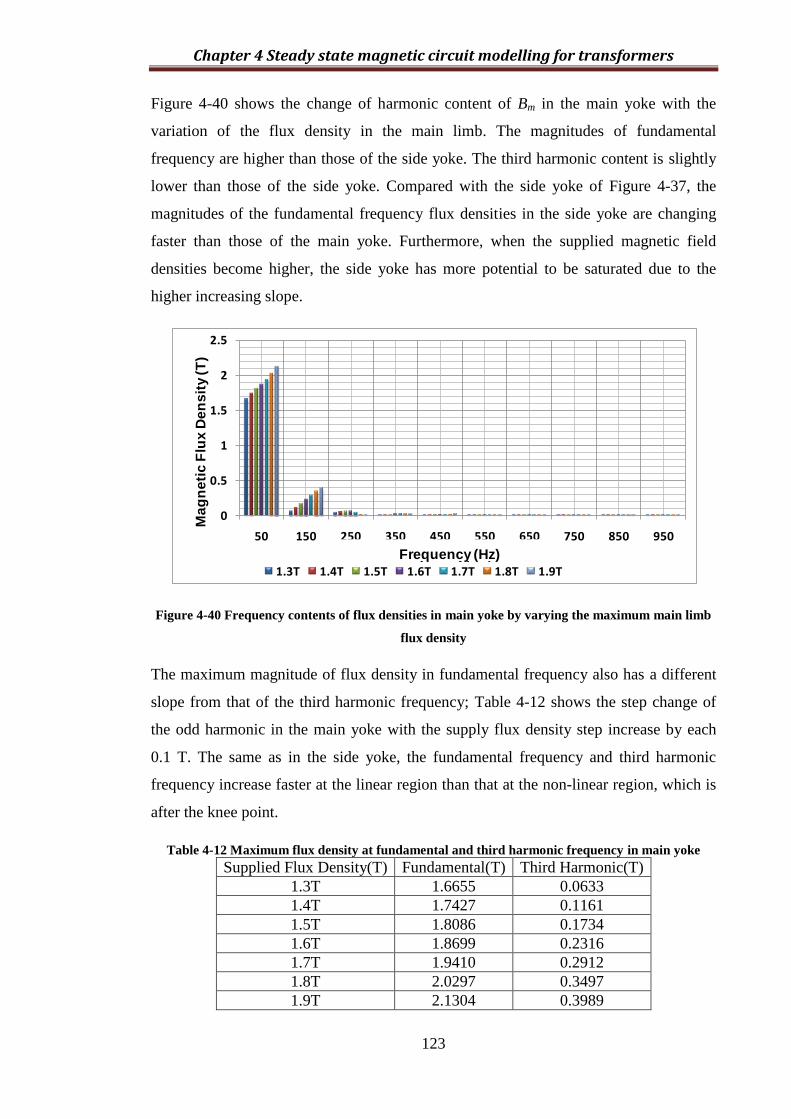
Chapter 4 Steady state magnetic circuit modelling for transformers
123
Figure 4-40 shows the change of harmonic content of Bm in the main yoke with the
variation of the flux density in the main limb. The magnitudes of fundamental
frequency are higher than those of the side yoke. The third harmonic content is slightly
lower than those of the side yoke. Compared with the side yoke of Figure 4-37, the
magnitudes of the fundamental frequency flux densities in the side yoke are changing
faster than those of the main yoke. Furthermore, when the supplied magnetic field
densities become higher, the side yoke has more potential to be saturated due to the
higher increasing slope.
Figure 4-40 Frequency contents of flux densities in main yoke by varying the maximum main limb
flux density
The maximum magnitude of flux density in fundamental frequency also has a different
slope from that of the third harmonic frequency; Table 4-12 shows the step change of
the odd harmonic in the main yoke with the supply flux density step increase by each
0.1 T. The same as in the side yoke, the fundamental frequency and third harmonic
frequency increase faster at the linear region than that at the non-linear region, which is
after the knee point.
Table 4-12 Maximum flux density at fundamental and third harmonic frequency in main yoke
Supplied Flux Density(T) Fundamental(T) Third Harmonic(T)
1.3T 1.6655 0.0633
1.4T 1.7427 0.1161
1.5T 1.8086 0.1734
1.6T 1.8699 0.2316
1.7T 1.9410 0.2912
1.8T 2.0297 0.3497
1.9T 2.1304 0.3989
0
0.5
1
1.5
2
2.5
50 150 250 350 450 550 650 750 850 950
Mag
en
tic
Flu
x D
en
sity
(T)
Frquency(Hz)1.3T 1.4T 1.5T 1.6T 1.7T 1.8T 1.9T
Frequency (Hz)
Ma
gn
eti
c F
lux
De
ns
ity (
T)

Chapter 4 Steady state magnetic circuit modelling for transformers
124
Figure 4-41 shows the phase angles of harmonics in the main yoke area. The
fundamental and 3rd
harmonic frequency phase angles have decreased which can also be
seen in Figure 4-39 for varying flux densities in the main limb. The phase angles of the
fifth harmonic frequency stay nearly the same until the core goes into deep saturation.
Figure 4-41 Phase angle contents of flux densities in main yoke by varying the maximum main limb
flux density
4.3.2 Impact of area
From the equation to calculate the side yoke flux of a three-phase five-limb transformer,
it can be seen that the magnetic flux density is associated with the maximum supplying
flux density, the permeability, the length, the cross-section area of each part of the
three-phase five-limb transformer core, which are the side yoke, the main yoke and the
main limb. The maximum supplying flux density will also influence the permeability, in
other words, these two conditions are coupled. The length of the main limb, the main
yoke and the side yoke is due to the winding length, the winding radius and the
insulation level. Moreover, it is now easy to understand that not only the permeability of
each part of transformer core contributes to the flux distribution, the cross-sections of
side yoke and main yoke also play an important role for the flux distribution.
Identifying the cross-section area of main limb 0.71805 m2
as 1 per unit, in order to let
all the flux have the return path, the cross-section areas of the side yoke and the main
yoke should be added together to be at least the same as that of the main limb. However,
the basic principle design is to make the transformer work reliably in normal conditions
-180
-120
-60
0
60
120
180
50 150 250
An
gle
(De
gre
e)
Frquency(Hz)1.3T 1.4T 1.5T 1.6T 1.7T 1.8T 1.9T
Frequency (Hz)

Chapter 4 Steady state magnetic circuit modelling for transformers
125
by using the least materials; normally the manufacturers use the ratio of 1:1 for the main
limb: (side yoke + main yoke).
Comparisons between the three groups are carried out by changing the supply magnetic
flux density, which is 1.1T at the liner region, 1.54T at the knee point and 1.9T at the
saturation region. In each group, the supply magnetic flux density is fixed by varying
the ratio of cross-section areas of the side yoke and the main yoke. The design rule is to
maximally use the materials characteristics; the core should work use near the knee area
under normal operating voltage. In this case, the knee area of the material is around 1.54
T. Varying the ratio of the cross-section area between the side yoke and the main yoke,
the sensitivity study on the impact of area ratio is carried out. Table 4-13 shows the ratio
variations of the cross-section area between the side yoke and the main yoke.
Table 4-13 Ratio variations of the cross section
Ratio Area of side yoke(m2) Area of main yoke(m
2)
0.5:0.5 0.359025 0.359025
0.45:0.55 0.3231225 0.3949275
0.4:0.6 0.28722 0.43083
0.35:0.65 0.2513175 0.4667325
0.3:0.7 21.5415 50.2635
Figure 4-42 and Figure 4-43 show that the flux density in the side yoke and main yoke
are at different area ratios and the supplying maximum flux density is 1.1 T. The
waveforms are all sinusoidal only when the amplitudes are different in both areas. The
amplitudes of the flux density are decreased with the increase of the ratio of the cross-
section area between the side yoke and the main yoke. The maximum magnitudes of Bm
in the side yoke are always lower than the supplied value of 1.1 T, on the other hand the
maximum magnitudes Bm of the main yoke are always higher than the supplied value of
1.1 T. For different area ratios, the Bm of the side yoke does not exhibit phase shifts
while the Bm of the main yoke shows some degree of phase shifts.

Chapter 4 Steady state magnetic circuit modelling for transformers
126
Figure 4-42 Side yoke flux densities waveforms at different area ratios at the supplying maximum
flux density of 1.1 T
Figure 4-43 Main yoke flux densities waveforms at different area ratios at the supplying maximum
flux density of 1.1 T
Table 4-14 shows the maximum magnitude of flux density at the side yoke and the main
yoke for different cross-section area ratios. From this table, it can also be seen that the
amplitudes of the magnetic flux density are decreased with the ratio of the cross-section
area between the side yoke and the main yoke.
Table 4-14 Maximum magnitude of flux density
Ratio Side yoke(T) Main yoke(T)
0.5:0.5 0.8522 1.4962
0.45:0.55 0.8433 1.4364
0.4:0.6 0.8346 1.3776
0.35:0.65 0.8261 1.3252
0.3:0.7 0.8177 1.2798
-2
-1.5
-1
-0.5
0
0.5
1
1.5
2
0 0.005 0.01 0.015 0.02 0.025 0.03 0.035 0.04
Ma
gne
tic
Flu
x D
en
sity
(T)
Time(s)0.5:0.5 0.45:0.55 0.4:0.6 0.35:0.65 0.3:0.7
-2
-1.5
-1
-0.5
0
0.5
1
1.5
2
0 0.005 0.01 0.015 0.02 0.025 0.03 0.035 0.04
Ma
gne
tic
Flu
x D
en
sity
(T)
Time(s)0.5:0.5 0.45:0.55 0.4:0.6 0.35:0.65 0.3:0.7

Chapter 4 Steady state magnetic circuit modelling for transformers
127
When increasing the supply magnetic flux density to the knee point of 1.54 T, the
magnetic flux density waveform of the side yoke and the main yoke are shown in Figure
4-44 and Figure 4-45. The waveforms are all distorted. The amplitude of the flux
density is decreased with the ratio of the cross-section area between the side yoke and
the main yoke. From Figure 4-45 it can be seen that the time for the flux density
waveform to be flat is increased with the decrease of the ratio of the cross-section area
between the side yoke and the main yoke. This also means that the total harmonic
content in the waveform is also increased.
Figure 4-44 Side yoke flux densities waveforms at different area ratios at the supplying maximum
flux density of 1.54 T
Figure 4-45 Main yoke flux densities waveforms at different area ratios at the supplying maximum
flux density of 1.54 T
-2
-1.5
-1
-0.5
0
0.5
1
1.5
2
0 0.005 0.01 0.015 0.02 0.025 0.03 0.035 0.04
Ma
gne
tic
Flu
x D
en
sity
(T)
Time(s)0.5:0.5 0.45:0.55 0.4:0.6 0.35:0.65 0.3:0.7
-2
-1.5
-1
-0.5
0
0.5
1
1.5
2
0 0.005 0.01 0.015 0.02 0.025 0.03 0.035 0.04
Ma
gne
tic
Flu
x D
en
sity
(T)
Time(s)0.5:0.5 0.45:0.55 0.4:0.6 0.35:0.65 0.3:0.7

Chapter 4 Steady state magnetic circuit modelling for transformers
128
Figure 4-46 and Figure 4-47, show that the magnitudes of fundamental frequency and
third harmonic in both the side yoke and the main yoke are decreased with the decrease
of the percentage ratio of the cross-section area between the side yoke and the main
yoke. This is because the increase of the main yoke area allows more flux to pass
through. In addition, both of the magnetic flux densities in the side yoke and main yoke
are decreased, due to the increase of percentage ratio of the cross-section area between
the side yoke and the main yoke. From this point of view, the higher the ratio between
the main yoke and the side yoke, the less likely the transformer will saturate. However,
the main yoke length is almost 2 times that of the side yoke; if the area of the main yoke
were increased, more materials would be required. It also increases the transformation
height and makes it harder to transport.
Figure 4-46 Frequency contents of flux densities in side yoke by varying ratio of cross-section at
knee region
Figure 4-47 Frequency contents of flux densities in main yoke by varying ratio of cross-section at
knee region
0
0.2
0.4
0.6
0.8
1
1.2
1.4
1.6
1.8
50 150 250 350 450 550 650 750 850 950
Mag
en
tic
Flu
x D
en
sity
(T)
Frquency(Hz)0.5:0.5 0.45:0.55 0.4:0.6 0.35:0.65 0.3:0.7
Frequency (Hz)
Ma
gn
eti
c F
lux
De
ns
ity (
T)
0
0.2
0.4
0.6
0.8
1
1.2
1.4
1.6
1.8
2
50 150 250 350 450 550 650 750 850 950
Ma
gen
tic
Flu
x D
en
sity
(T
)
Frquency(Hz)0.5:0.5 0.45:0.55 0.4:0.6 0.35:0.65 0.3:0.7
Frequency (Hz)
Ma
gn
eti
c F
lux
De
ns
ity (
T)

Chapter 4 Steady state magnetic circuit modelling for transformers
129
Continuing to increase the supply magnetic flux density into saturation region as 1.9 T,
the flux density waveform of the side yoke and the main yoke are shown in Figure 4-48
and Figure 4-49. The waveforms of the magnetic flux density are all distorted. The
change in the flux density in the side yoke is not much; however the flux density in the
main yoke is changed to a better sinusoidal waveform by decreasing the ratio of the
cross-section between the side yoke and the main yoke.
Figure 4-48 Side yoke flux densities waveforms at different area ratios at the supplying maximum
flux density of 1.9 T
Figure 4-49 Main yoke flux densities waveforms at different area ratios at the supplying maximum
flux density of 1.9 T
Figure 4-50 shows that the maximum magnitudes of fundamental frequency and third
harmonic in the side yoke do not change much by decreasing the percentage ratio of the
cross-section area between the side yoke and the main yoke. In addition, the fifth,
-2
-1.5
-1
-0.5
0
0.5
1
1.5
2
0 0.005 0.01 0.015 0.02 0.025 0.03 0.035 0.04
Ma
gne
tic
Flu
x D
en
sity
(T
)
Time(s)0.5:0.5 0.45:0.55 0.4:0.6 0.35:0.65 0.3:0.7
-2
-1.5
-1
-0.5
0
0.5
1
1.5
2
0 0.005 0.01 0.015 0.02 0.025 0.03 0.035 0.04
Ma
gne
tic
Flu
x D
en
sity
(T)
Time(s)0.5:0.5 0.45:0.55 0.4:0.6 0.35:0.65 0.3:0.7

Chapter 4 Steady state magnetic circuit modelling for transformers
130
seventh and ninth harmonics appear. This is because the side yoke has already been
deep saturated; this is why we cannot see too much difference between them.
Figure 4-50 Frequency contents of flux densities in side yoke by varying ratio of cross-section at
nonlinear region
Figure 4-51 shows that the maximum magnitudes of fundamental frequency and third
harmonic are decreased with the increase of ratio of the cross-section area between the
side yoke and the main yoke.
Figure 4-51 Frequency contents of flux densities in main yoke by varying ratio of cross-section at
nonlinear region
0
0.5
1
1.5
2
2.5
50 150 250 350 450 550 650 750 850 950
Ma
gen
tic
Flu
x D
en
sity
(T
)
Frquency(Hz)0.5:0.5 0.45:0.55 0.4:0.6 0.35:0.65 0.3:0.7
Frequency (Hz)
Ma
gn
eti
c F
lux
De
ns
ity (
T)
0
0.5
1
1.5
2
2.5
50 150 250 350 450 550 650 750 850 950
Ma
gen
tic
Flu
x D
en
sity
(T
)
Frquency(Hz)0.5:0.5 0.45:0.55 0.4:0.6 0.35:0.65 0.3:0.7
Frequency (Hz)
Ma
gn
eti
c F
lux
De
ns
ity (
T)
Chapter 4 Steady state magnetic circuit modelling for transformers
131
4.4 Case 3: GIC Study---sensitivity on unbalanced
situation
As mentioned in the literature review, the cycle of solar wind is around eleven years.
The last famous one (which led the Canadian power system to black out) is 22 years old,
and this year solar wind is active again. Consequently, the risks of transformer failure
need to be considered.
The solar winds will disturb the geomagnetic field, and then shift the potential of the
surface voltage up. The frequency of the created voltage is around 0.1 Hz, which will
look like DC supplied into the power system grid.
4.4.1 Impact of DC supply level
Taking the three-limb core transformer as an example, the investigation is carried out on
the impact of the DC supply level on transformer saturation by varying the peak value
of the flux density in the main limb as at the linear region, knee point and non-linear
region; the magnetising current and the flux density at the main yoke and the tank are
calculated.
4.4.1.1 Sensitivity study on linear region with DC situation
The supplied three-phase AC voltage is 70% of the rated voltage, which can warrant the
transformer working under the linear region. The DC supply, which is in the unit of flux,
Wb, varies at 0.1 Wb, 0.15 Wb or 0.2 Wb.
Figure 4-52 shows the line magnetising current waveforms varying by the DC supply
level. The round dotted lines represent the magnetising currents under the DC supply
level as zero, the dash lines represent the magnetising currents under the DC supply
level as 0.1 Wb, the dash dotted lines represent the magnetising currents under the DC
supply level as 0.15 Wb, the dash long lines represent the magnetising currents under
the DC supply level as 0.2 Wb. It can be seen that the line magnetising currents are
follow the sinusoidal waveform until the DC supply level reaches 0.15Wb. When the
DC supply level is increased to 0.2 Wb, the current waveforms are distorted.
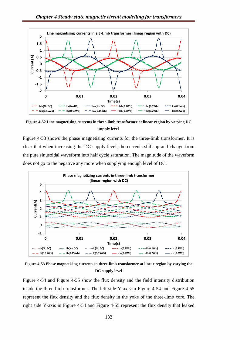
Chapter 4 Steady state magnetic circuit modelling for transformers
132
Figure 4-52 Line magnetising currents in three-limb transformer at linear region by varying DC
supply level
Figure 4-53 shows the phase magnetising currents for the three-limb transformer. It is
clear that when increasing the DC supply level, the currents shift up and change from
the pure sinusoidal waveform into half cycle saturation. The magnitude of the waveform
does not go to the negative any more when supplying enough level of DC.
Figure 4-53 Phase magnetising currents in three-limb transformer at linear region by varying the
DC supply level
Figure 4-54 and Figure 4-55 show the flux density and the field intensity distribution
inside the three-limb transformer. The left side Y-axis in Figure 4-54 and Figure 4-55
represent the flux density and the flux density in the yoke of the three-limb core. The
right side Y-axis in Figure 4-54 and Figure 4-55 represent the flux density that leaked
-2
-1.5
-1
-0.5
0
0.5
1
1.5
2
0 0.01 0.02 0.03 0.04
Cu
rre
nt
(A)
Time(s)
Line magnetising currents in a 3-Limb transformer (linear region with DC)
Iab(No DC) Ibc(No DC) Ica(No DC) Iab(0.1Wb) Ibc(0.1Wb) Ica(0.1Wb)
Iab(0.15Wb) Ibc(0.15Wb) Ica(0.15Wb) Iab(0.2Wb) Ibc(0.2Wb) Ica(0.2Wb)
-1
0
1
2
3
4
5
0 0.01 0.02 0.03 0.04
Cu
rre
nt(
A)
Time(s)
Phase magnetizing currents in three-limb transformer (linear region with DC)
Ia(No DC) Ib(No DC) Ic(No DC) Ia(0.1Wb) Ib(0.1Wb) Ic(0.1Wb)
Ia(0.15Wb) Ib(0.15Wb) Ic(0.15Wb) Ia(0.2Wb) Ib(0.2Wb) Ic(0.2Wb)

Chapter 4 Steady state magnetic circuit modelling for transformers
133
out of the three-limb core. The flux density and filed intensity would be increased at the
yoke area as the DC supply level increases, but not too much. The positive magnitude of
the flux density is changed from 1.2 T to 1.4 T, and the positive magnitude of the field
intensity is changed from 22 A/m to 25 A/m. However, the leak out flux density and
field intensity suddenly increased about twice the rate.
Figure 4-54 Flux densities distributions in three-limb transformer at linear region by varying the
DC supply level
Figure 4-55 Field intensities distributions in three-limb transformer at linear region by varying the
DC supply level

Chapter 4 Steady state magnetic circuit modelling for transformers
134
4.4.1.2 Sensitivity study on knee area with DC situation
The supplied three-phase AC voltage is the rated voltage, which can warrant the
transformer working under the linear region similar to the linear region one, the DC
supply, which is in the unit of flux, Wb, varies at 0.1 Wb, 0.15 Wb and 0.2 Wb.
The same experience can be obtained in the last section, the magnitude of the line
current can change and there is no magnitude offset shift, the three-phase currents still
follow the balanced situation. As a result, only the phase currents are calculated.
Figure 4-56 and Figure 4-57 show phase current waveforms. The magnetising current is
much more sensitive towards DC supply compared with the linear region. When the DC
supply is 0.15 Wb, the current has already shown transformer half cycle saturation, and
furthermore increasing the DC supply results in the dramatic increase of the magnitude
of the current.
Figure 4-56 Phase magnetising currents in three-limb transformer (No DC, 0.1 Wb)
-2
0
2
4
6
8
10
0 0.01 0.02 0.03 0.04
Cu
rre
nt
(A)
Time(s)
Phase magnetising currents in a 3-Limb transformer (Knee region with DC)
Ia(No DC) Ib(No DC) Ic(No DC) Ia(0.1Wb) Ib(0.1Wb) Ic(0.1Wb)

Chapter 4 Steady state magnetic circuit modelling for transformers
135
Figure 4-57 Phase magnetising currents in three-limb transformer (0.15 Wb, 0.2 Wb)
Figure 4-58 and Figure 4-59 show that the flux density and the filed intensity. The X-
axis and the Y-axis styles are all the same as the previous figures. It can be seen that the
flux density waveforms start to become distorted and the flat part of the saturation
period becomes longer when increasing the DC supply level. In addition, the flux
density escaped to the tank is increased to 0.14 T. The field intensity is much more
distorted compared with the flux density waveform.
Figure 4-58 Flux density distributions in three-limb transformer by varying the DC supply level
0
200
400
600
800
1000
1200
1400
1600
1800
2000
0 0.01 0.02 0.03 0.04
Cu
rre
nt
(A)
Time(s)
Phase magnetising currents in a 3-Limb transformer (Knee region with DC)
Ia(0.15Wb) Ib(0.15Wb) Ic(0.15Wb) Ia(0.2Wb) Ib(0.2Wb) Ic(0.2Wb)
0
0.02
0.04
0.06
0.08
0.1
0.12
0.14
0.16
-2
-1.5
-1
-0.5
0
0.5
1
1.5
2
0 0.01 0.02 0.03 0.04
B(T
)
B(T
)
Time(s)
Flux Distribution in three-limb transformer(Knee region with DC)
Bbc(0.1Wb) Bab(0.1Wb) Bab(0.15Wb) Bbc(0.15Wb) Bab(0.2Wb) Bbc(0.2Wb)
Blt(0.1Wb) Brt(0.1Wb) Blt(0.15Wb) Brt(0.15Wb) Blt(0.2Wb) Brt(0.2Wb)

Chapter 4 Steady state magnetic circuit modelling for transformers
136
Figure 4-59 Field intensity distributions in three-limb transformer by varying the DC supply level
4.4.1.3 Sensitivity study on non-linear region with DC situation
The supplied three-phase AC voltage is 120% of rated voltage, which can warrant the
transformer working under the non-linear region. The same as the previous two cases,
the DC supply which is in the unit of flux, Wb, varies at 0.1 Wb, 0.15 Wb and 0.2 Wb.
Instead of showing the phase current waveforms, Table 4-15 shows the peak value
results of the phase current in all the three simulation cases. It can be seen that, the
higher the working point of the transformer, the more sensitive it is towards the DC
supply.
Table 4-15 Peak values of the phase currents for different cases
DC(Wb) Ia(A) Ib(A) Ic(A)
Linear
0.1 2.564749 2.614067 2.564751
0.15 3.841559 3.919921 3.841561
0.2 5.373061 5.477727 5.373062
Knee
0.1 4.653478 4.687275 4.653488
0.15 48.48069 48.51229 48.4807
0.2 624.8655 624.9169 624.8655
Non-Linear
0.1 4021.98 4022.017 4021.98
0.15 39118.42 39118.55 39118.42
0.2 329004.1 329004.3 329004.1
Figure 4-60 and Figure 4-61 show the flux density and field intensity distribution.
Compared with the case of rated voltage supplied, the magnitudes of both parameters
are increased and the harmonic contents are more serious. The saturation period is
longer which can be seen from the flat part of the of flux density yoke in Figure 4-60.
0
50
100
150
200
250
-40
-20
0
20
40
60
80
100
0 0.01 0.02 0.03 0.04
H(A
/m)
H(A
/m)
Time(s)
Field intensity in three-limb transformer(Knee region with DC)
Hab(0.1Wb) Hbc(0.1Wb) Hab(0.15Wb) Hbc(0.15Wb) Hab(0.2Wb) Hbc(0.2Wb)
Hlt(0.1Wb) Hrt(0.1Wb) Hlt(0.15Wb) Hrt(0.15Wb) Hlt(0.2Wb) Hrt(0.2Wb)

Chapter 4 Steady state magnetic circuit modelling for transformers
137
Figure 4-60 Flux density distribution in the three-limb transformer
Figure 4-61 Field intensity distribution in the three-limb transformer
From the investigation above, it can be seen that the higher the working point of the
transformer, the higher the risk of saturation the transformer would have when it meets
the DC supply. The five-limb transformer has the similar trend as the three-limb core
transformer.
4.5 Summary
In this chapter, the transformer core structure influence on the magnetising current and
the transformers response to DC bias or GIC events has been successfully identified.
0
0.05
0.1
0.15
0.2
-2
-1.5
-1
-0.5
0
0.5
1
1.5
2
0 0.01 0.02 0.03 0.04
B(T
)
B(T
)
Time(s)
Flux distribution in three-limb transformer(Nonlinear region with DC)
Bbc(0.1Wb) Bab(0.1Wb) Bab(0.15Wb) Bbc(0.15Wb) Bab(0.2Wb) Bbc(0.2Wb)
Blt(0.1Wb) Brt(0.1Wb) Blt(0.15Wb) Brt(0.15Wb) Blt(0.2Wb) Brt(0.2Wb)
0
50
100
150
200
250
300
-100
-50
0
50
100
150
200
250
300
350
0 0.01 0.02 0.03 0.04
H(A
/m)
H(A
/m)
Time(s)
Field intensity in three-limb transformer(Nonlinear region with DC)
Hab(0.1Wb) Hbc(0.1Wb) Hab(0.15Wb) Hbc(0.15Wb) Hab(0.2Wb) Hbc(0.2Wb)
Hlt(0.1Wb) Hrt(0.1Wb) Hlt(0.15Wb) Hrt(0.15Wb) Hlt(0.2Wb) Hrt(0.2Wb)
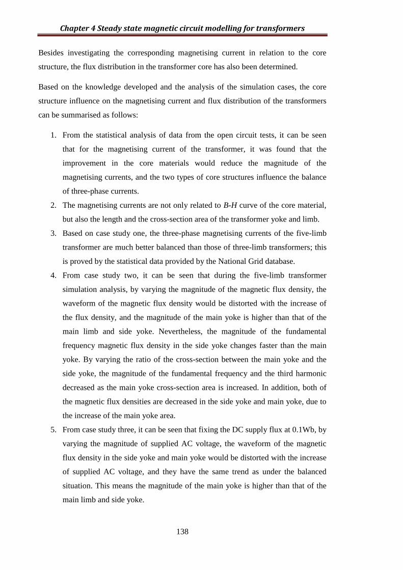
Chapter 4 Steady state magnetic circuit modelling for transformers
138
Besides investigating the corresponding magnetising current in relation to the core
structure, the flux distribution in the transformer core has also been determined.
Based on the knowledge developed and the analysis of the simulation cases, the core
structure influence on the magnetising current and flux distribution of the transformers
can be summarised as follows:
1. From the statistical analysis of data from the open circuit tests, it can be seen
that for the magnetising current of the transformer, it was found that the
improvement in the core materials would reduce the magnitude of the
magnetising currents, and the two types of core structures influence the balance
of three-phase currents.
2. The magnetising currents are not only related to B-H curve of the core material,
but also the length and the cross-section area of the transformer yoke and limb.
3. Based on case study one, the three-phase magnetising currents of the five-limb
transformer are much better balanced than those of three-limb transformers; this
is proved by the statistical data provided by the National Grid database.
4. From case study two, it can be seen that during the five-limb transformer
simulation analysis, by varying the magnitude of the magnetic flux density, the
waveform of the magnetic flux density would be distorted with the increase of
the flux density, and the magnitude of the main yoke is higher than that of the
main limb and side yoke. Nevertheless, the magnitude of the fundamental
frequency magnetic flux density in the side yoke changes faster than the main
yoke. By varying the ratio of the cross-section between the main yoke and the
side yoke, the magnitude of the fundamental frequency and the third harmonic
decreased as the main yoke cross-section area is increased. In addition, both of
the magnetic flux densities are decreased in the side yoke and main yoke, due to
the increase of the main yoke area.
5. From case study three, it can be seen that fixing the DC supply flux at 0.1Wb, by
varying the magnitude of supplied AC voltage, the waveform of the magnetic
flux density in the side yoke and main yoke would be distorted with the increase
of supplied AC voltage, and they have the same trend as under the balanced
situation. This means the magnitude of the main yoke is higher than that of the
main limb and side yoke.

Chapter 4 Steady state magnetic circuit modelling for transformers
139
Although the manufacturer provides the RMS values of the magnetising currents, the
information is not sufficient to understand the flux distribution and the core situation.
The recommendation is made for the manufacturer to provide more detailed
magnetising current waveforms.
However, all the analyses above are based on some assumptions, the losses and the
joints of the transformer core are not considered, the model is good for analysis of
individual transformer flux distributions and magnetising currents; however it is not
appropriate to investigate the GIC or other core saturation events of the whole network
influence. Therefore, the next chapter will look at the influences regarding the network.

Chapter 5 GIC magnetic and electrical circuit modelling
140
Chapter 5 GIC magnetic and
electrical circuit modelling
5.1 Introduction
In Chapter 4, the influence of the transformer core structure on magnetising currents and
flux distributions was discussed. In addition, the investigation is conducted on both the
balanced and unbalanced situations in order to understand parameters which influence
the flux distribution.
In reality, a three single-phase transformers bank is normally used as generator
transformers, three-phase five-limb transformers are extensively used as interconnection
transformers to connect two transmission voltage levels; three-phase three-limb
transformers are the most frequent form, which are extensively used in transmission
systems and distribution systems. Therefore, it is necessary to model the individual
system under study in order to understand the influences of system parameters and the
transformer structure.
This chapter will set out to evaluate the power system and transformer factors that may
affect the magnetising current level and its risk when a transformer meets the DC bias
situations or GIC events. The transformer structures and the system parameters will be
examined for their influences on GIC. Both cases of the DC only and AC plus DC
voltage supply are studied. The DC only case is used to illustrate the core saturation
process, which clearly shows the stages of the growing process of primary current
during a GIC event. However, in reality, the system works under the AC source, and the
AC plus DC voltage supply case is more realistic, since the core works in the knee area
so it quickly saturates and the envelope of the current is more realistic.
5.2 Case 1: GIC effect on single phase transformer
5.2.1 Single-phase model
The transformer data used are from an existing three-limb distribution transformer,
because no single phase transformer data are provided. The voltage level of the single

Chapter 5 GIC magnetic and electrical circuit modelling
141
phase transformer is assumed to be the same as the real three-phase transformer which
is 132/33 kV. The data used for the transformer modelling are shown in previous
chapter Table 4-1.
According to the open circuit and short circuit test report data in Table 5-1, the
equivalent resistance and inductance of the core and the winding can be obtained. The
short circuit test is carried out on the high voltage side i.e. 132 kV for a rated current
with low magnitude; while the open circuit test is carried out on the low voltage side i.e.
33 kV for a rated voltage with low magnitude.
Table 5-1 132/33 kV transformer test report data
Short circuit test Open circuit test
Voltage
(V)
Current
(A)
Losses
(kW)
No load
voltage(V)
Average
current(A)
No load
loss(kW)
29628 378.1 279.9 29702 0. 643 23.61
/ / / 33005 0.977 29.64
/ / / 36296 1.8133 37.62
From experience, if there is no specific value provided by the manufacturer, then the
distribution of the winding impedance at primary and secondary sides will be the same,
50% of the impedance. The calculation equations are the following:
. .
1* * (5.1)
2s
p w s w bb
PR R Z
S
2 2
. . .
1* ( ) (5.2)
2H
p w s w p ws
VX X R
I
.. . (5.3)
2p w
p w s w
XL L
f
2
(5.4)Hb
b
VZ
S
21* (5.5)
3o
co
VR
P
All the symbols of the equations are shown in Table 5-2.

Chapter 5 GIC magnetic and electrical circuit modelling
142
Table 5-2 Symbol explanations for the calculation of transformer parameters
Winding resistance per phase on the
primary side Short circuit test losses
Winding resistance per phase on the
secondary side Power base
Winding reactance per phase on the
primary side Primary side voltage
Winding reactance per phase on the
secondary side Short circuit test current
Winding inductance per phase on the
primary side f Frequency of the system
Winding inductance per phase on the
secondary side Impedance base on the primary side
Core resistance per phase 100% voltage in open circuit test
100% voltage open circuit test losses
Then all the parameters which are used in the lumped-element transformer model can be
calculated. And the calculated parameter values are shown in Table 5-3.
Table 5-3 Values of transformer model parameters
To represent the single-phase transformer core characteristics, for the purpose of
illustration only, the three-limb transformer core characteristics are used. Figure 5-1
shows the core characteristics λ-I curve, where the λ is the flux linkage of the
transformer in Wb, and I is the magnetising current in Amp.
Figure 5-1 Core λ-I curve from the three-phase transformer

Chapter 5 GIC magnetic and electrical circuit modelling
143
The curve shown in Figure 5-1 is fitted by using the open circuit test which is based on
the 90%, 100% and 110% supplied voltages and corresponding magnetising currents.
Then a three single-phase transformer model can be built in ATPDraw for investigating
the DC bias or GIC events. The model is built as a lumped parameters model which
includes the resistances and inductances of primary winding and secondary winding
(Rp.w, Lp.w, Rs.w, Ls.w), the resistance and non-linear inductance of the transformer core
(Rc, Lc). One of single-phase transformer models is shown in Figure 5-2.
Figure 5-2 Single phase transformer model
The difference between the YNd connected transformers and YNy connected
transformers of the no load situation is due to the fact that the zero sequence induced
current can pass through the delta windings but not the star-connected open circuit
windings. So the transformer winding connections as YNd and YNy should have
different responses when both of them meet the GIC or DC bias situation.
To investigate the influences of two different winding connections three single-phase
transformer models are built and the simulation results are presented and discussed in
the following sections.
5.2.2 Simulation of DC only supply
The simulation is designed in such a way that a step-by-step approach is used. The first
step is conducted to supply a DC voltage into the primary side of the single phase
transformer to investigate the influence of DC bias or GIC. As the typical range of GIC
value is from 10 to 15 V [70], a 10 V DC voltage source is used. There are two key
geophysical factors controlling the earth surface potential level, which are: ground
conductivity structure and geomagnetic latitude [84].
The single phase transformer model connected with DC voltage source is shown in
Figure 5-3.

Chapter 5 GIC magnetic and electrical circuit modelling
144
Figure 5-3 Single phase transformer simulation model in ATP
The three single-phase transformers are connected together by using delta connected
secondary windings under an open circuited situation which is shown in Figure 5-4. The
supplied voltage is a DC source, and then the DC current or zero sequence current
would be circulating in the transformer delta connected windings. The results are shown
in Figure 5-5.
Figure 5-4 Three single-phase transformer bank simulation model in ATP

Chapter 5 GIC magnetic and electrical circuit modelling
145
(a)
(b)
Figure 5-5 (a) Primary side current and flux under DC excitation-full waveforms
(b) Primary side current under DC excitation-zoomed in waveform
Figure 5-5 shows the primary side current and the flux waveform, the red line represents
the primary side current and the green line represents the flux linkage. It can be seen
that the primary current has a 'two-step function' waveform, and the flux has a 'one-step
function' waveform. In order to conveniently explain its behaviour, the waveform of the
current is divided into three stages as indicated in Figure 5-5.
Figure 5-5 (b) shows that the primary side current waveform of Figure 5-5 (a) is
separated into three parts and each part is zoomed. Each stage is named in accordance
with its own property. However, it is not quantificational defined so there are no
definite boundaries between the two adjacent stages.
It can be seen in Figure 5-5 (b) that, the step-response stage is the first stage that the
primary current has experienced under the GIC. Because the circuit is structured as the
inductance and resistance, from the fundamentals of electric circuits; it is known that the
behaviour of the primary current would start as the step-response-like. The pseudo-flat
stage comes after the step-response stage; and the waveform looks flat in Figure 5-5 (a),
but when it is zoomed in, it is in fact not flat. The saturation stage comes after the
pseudo-flat stage; and the current is increased quickly and then stabilised at this stage.
This is mainly due to the saturation characteristics of the non-linear inductance of the
transformer core.
Flux(W
b)C
urr
en
t(A
)
Time(s)
Stage I
Stage IIIStage II
Step-response stage Pseudo-flat stage Saturation stage
Cu
rre
nt(
A)

Chapter 5 GIC magnetic and electrical circuit modelling
146
The equivalent circuit of the whole circuit can be represented in Figure 5-6 which can
help to understand the “two-step function” waveform of the primary current.
Figure 5-6 Equivalent circuit of the simulation model
The secondary delta winding impedance is referred to the primary side and paralleled
with Rc and Lc.
The equivalent circuit works as long as the transformer is working properly. It means
that the current flowing into the transformer core, i.e. the non-linear inductance in this
case must vary with real time to make sure the secondary winding impedance can be
seen by the whole circuit.
The beginning of the supply DC only voltage which is the step-response stage; a current
is produced and tends to approach the first stable DC current value in the transformer
core non-saturated situation. However, due to the effect of the inductance, it takes time
for the current to grow from zero to a stable value. During this stage, the transformer
core is working at the linear region and the inductance and resistance of the core both
have with large values compared with the winding inductance and resistance, and also
as the core impedance is parallel with the secondary winding impedance, the core
impedance can then be omitted. The equivalent circuit can therefore be simplified as
shown in Figure 5-7.
Figure 5-7 Simplified equivalent circuit at step-response stage in YNd connection
Once the circuit is determined, the time constant and the final value for the step
response can be calculated by using (5.6).

Chapter 5 GIC magnetic and electrical circuit modelling
147
. . . .( )* ( ) (5.6)o p w s w p w s wdiV R R i L L
dt
By solving the differential equation above, the current can be obtained as,
. .
. .
*
. .
*(1 ) (5.7)
p w s w
p w s w
R Rt
L Lo
p w s w
Vi e
R R
Then the time constant and the final stable value are calculated as,
. .
. .
0.0720.2371 (5.8)
0.301
p w s w
p w s w
L L Ht s
R R
. .
1016.6 (5.9)
2*0.301
oo
p w s w
V Vi A
R R
A comparison between the theoretical calculations with the simulation results is shown
in Figure 5-8. The simulation results show that the final stable value is 16.6 A and the
time constant is 0.2371 s, which coincides with the calculation values. As a final point
during the step-response stage, only the winding resistances would influence the results,
and the transformer core impedance can be ignored.
Figure 5-8 Time constant and the final value of the step response current
For the second stage which is the pseudo-flat stage, it can be seen that the primary side
current has changed slightly. As long as there is some voltage drop in the core, there
will be a current flowing through the core resistance and inductance, the secondary delta
T=0.2371sI=(1 - e-1)Io=10.49A
Io=16.6A
Time(s)
Cu
rre
nt(
A)

Chapter 5 GIC magnetic and electrical circuit modelling
148
connected winding impedance still needs to be taken into account as the transformer
still works and follows the fundamental theory.
Due to the DC voltage drop on the transformer core which is around a half of the source
voltage, the flux is accumulated in the transformer core. As we know, for the single
phase transformer all the DC flux would be circulated inside of the core. In addition,
with the DC flux growing, the working point of the non-linearity of the inductance
gradually shifts up and approaches the knee area.
In this process, the value of the non-linear inductance decreases slowly and the current
increases slightly. Consequently, the primary current, as the sum of the secondary
current, the core resistance current and core inductance current, increases slightly.
Figure 5-9 indicates the variation of the current of the non-linear inductance and the
primary current under its influence.
Figure 5-9 Primary current and core current at the pseudo-flat stage
It can be seen that during this stage both the primary and non-linear inductance currents
have changed. Therefore, the change makes sure that the transformer is still working
properly; because the flux in the core also varies by the time the induced voltage
appears in the secondary side of the transformer. At the end of pseudo-flat stage, the
flux reaches the knee area and the value of the non-inductance starts to change swiftly.
Primary current
Core current
Cu
rre
nt(
A)
Time(s)
Cu
rre
nt(
A)
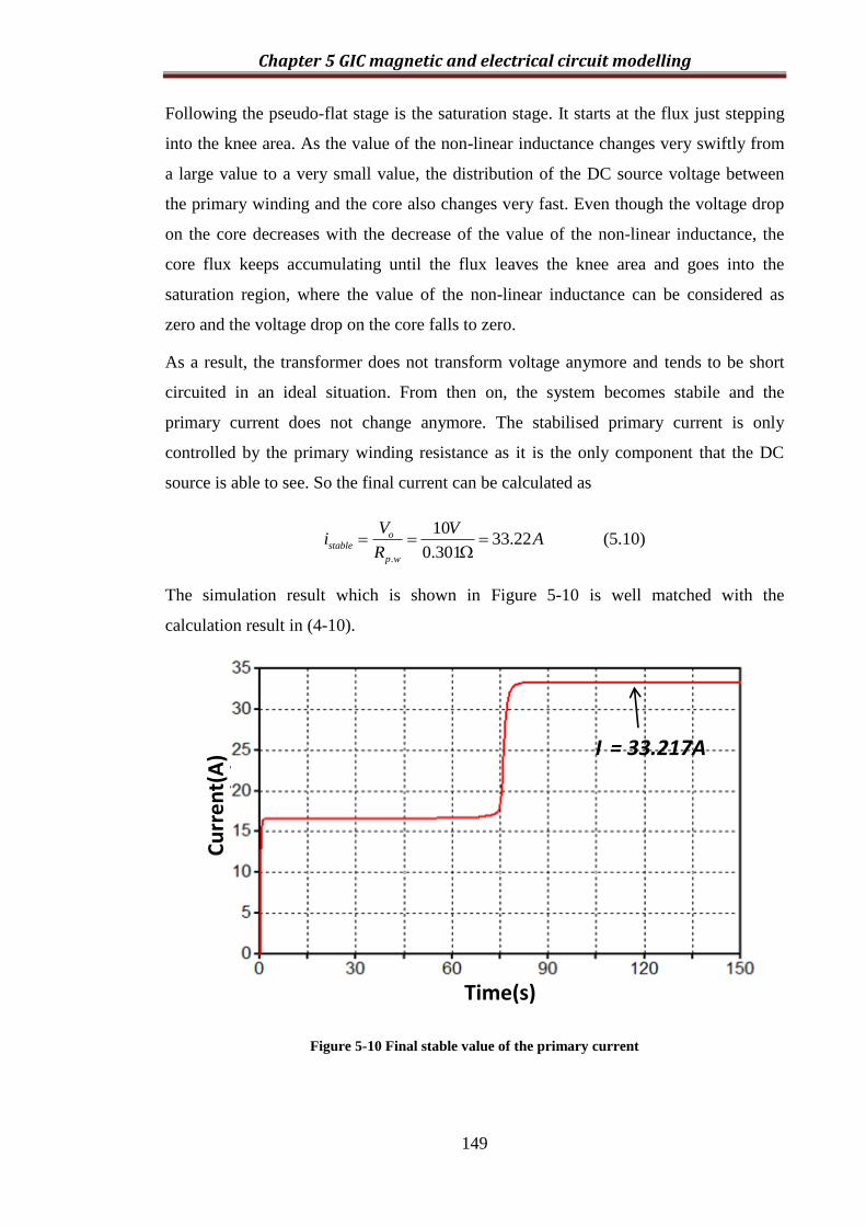
Chapter 5 GIC magnetic and electrical circuit modelling
149
Following the pseudo-flat stage is the saturation stage. It starts at the flux just stepping
into the knee area. As the value of the non-linear inductance changes very swiftly from
a large value to a very small value, the distribution of the DC source voltage between
the primary winding and the core also changes very fast. Even though the voltage drop
on the core decreases with the decrease of the value of the non-linear inductance, the
core flux keeps accumulating until the flux leaves the knee area and goes into the
saturation region, where the value of the non-linear inductance can be considered as
zero and the voltage drop on the core falls to zero.
As a result, the transformer does not transform voltage anymore and tends to be short
circuited in an ideal situation. From then on, the system becomes stabile and the
primary current does not change anymore. The stabilised primary current is only
controlled by the primary winding resistance as it is the only component that the DC
source is able to see. So the final current can be calculated as
.
1033.22 (5.10)
0.301
ostable
p w
V Vi A
R
The simulation result which is shown in Figure 5-10 is well matched with the
calculation result in (4-10).
Figure 5-10 Final stable value of the primary current
I = 33.217A
Cu
rre
nt(
A)
Time(s)

Chapter 5 GIC magnetic and electrical circuit modelling
150
As the flux is totally contributed by the DC voltage source, it can be calculated by using
the formula: 0dE
dt
, E is the voltage drop on the transformer core which results in the
total flux accumulated by the DC source.
Assuming that the 110% rated voltage can saturate the transformer core, and then the
saturation flux can be calculated as0
110%* ( 2 sin )3
rateds
Vt dt
.
The time for the saturation of the core and also for the primary current to become stabile
can be approximately calculated as stE
. In this case the saturation time is 75.5 s.
The simulation results are shown in Figure 5-11 which include the flux linkage and the
primary current waveforms. It can be seen that the saturation time is 82.4 s which is a
little bit greater than the theoretically calculated result.
Figure 5-11 Core flux and primary current
The difference between the simulation results and the calculation results are mainly due
to two reasons; the first is that the knee area is simplified as the cross point of the two
straight lines, one represents the linear region and the other saturation region; and the
second is that the voltage drop on the transformer core is assumed as a constant value
before the transformer is saturated. In the calculation, the flux is approximated to
accumulate a consistent speed even in the knee area, but the growing speed of flux in
the knee area is actually slower.
Primary current
Core flux
t = 82.4s
Cu
rre
nt(
A)
Time(s)
Flux(W
b)

Chapter 5 GIC magnetic and electrical circuit modelling
151
5.2.3 Winding connection influence
For three single-phase transformers which are connected as YNy, it can be seen that
there is no mutual coupling between any of them, and the zero sequence current cannot
be passed to the secondary side windings. So a single phase model can be used to
represent the situation of the three single-phase transformers (transformers bank).
Therefore the simulation of DC voltage supply is carried out by using the model which
is shown in Figure 5-12.
Figure 5-12 Simplified three single-phase transformers model in ATPDraw
The simulation result is shown in Figure 5-13. It can be seen that the step-response
stage disappears and the other two stages remain. The primary current stabilises when
the core flux stops growing and reaches saturation. The saturation time is around 42 s
which is half the saturation time of the YNd three single-phase transformers bank (82.4
s).
Figure 5-13 Core flux and primary current in the simulation for YNy three single-phase
transformers bank
Since the primary winding impedance in series with the core impedance is smaller than
the core impedance, almost all of the DC voltage would drop onto the core impedance
until the core is saturated and behaves as short-circuited. In addition, the step response
Cu
rre
nt(
A)
Time(s)
Flux(W
b)Primary current
Core flux
t = 42s

Chapter 5 GIC magnetic and electrical circuit modelling
152
should still exist but the total system inductance is the winding plus the core
inductances which are equal to a large value, then the increasing time of the current is
too long to be seen. Figure 5-14 shows the simplified equivalent circuit at the step-
response stage in YNy connection.
Figure 5-14 Simplified equivalent circuit at step-response stage for YNy connection
Before the first stabile point appears, the core has already been saturated and the current
would rise again to reach the final stabile point; so the step response would not be
observed in this case. Also, almost all of the supplied voltage drops onto the core
inductance instead of half the voltage as in the YNd case, the flux accumulating speed
doubles and the time for saturation is halved compared with the YNd connected
transformer.
To conclude, the primary current presents a ‘single-step function’ waveform in the YNy
connection situation instead of a ‘two-step function’ waveform as in the YNd
connection. Since the step-response stage is not observed, the pseudo-flat stage and the
saturation stage show up; however the saturation time will be approximately half that in
the simulation for the YNd three single-phase transformers bank.
For the three single-phase transformers bank, the key parameters which influence the
transformer behaviour under the GIC events include the level of DC voltage supply, the
value of winding resistance, the value of winding inductance and the non-linear
characteristics of the core.
5.2.4 Transformer core characteristic influence
From the previous section, it can be seen that the core characteristics can influence the
results. Therefore the core characteristics, which are the non-linear inductance of the
core, are varied so that we can understand its influence. The single phase transformer
model in Figure 5-3 has been used for the simulation studies. The resistance of 0.5 Ω
and inductance of 100 mH added at the primary side, which is between the DC voltage

Chapter 5 GIC magnetic and electrical circuit modelling
153
source and the transformer, represent the system’s resistance and inductance. The 10 V
DC voltage is supplied as the source.
5.2.4.1 Forward and backward shifting
The λ-I curve of the non-linear inductance is modified by changing the non-linear
characteristics settings. The λ-I curve is defined by 31 flux/current points, and it can be
modified by changing the current value of each point with the corresponding flux value
maintained. In this way, the maximum flux that the core inductance can reach is
maintained while the curve is shifted backward by reducing the current values or shifted
forwards by increasing them. This modification is to simulate different materials which
are used to build the transformer core.
In the simulations, two extra λ-I curves are generated based on the original one. Figure
5-15 shows two generated curves and the original λ-I curve.
Figure 5-15 λ-I curves (a): Three curves in one figure (b): Knee areas of three curves
The original one is given as the green line, the backward shifted one is given as the red
line and the forward shifted one is given as the blue line. The modifications attempt to
represent different situations; i.e. the backward shifted curve represents the easiest case
for the core to saturate, because it needs the least current to reach the maximum flux. By
contrast the forward shifted curve is the hardest to go into saturation since it requires the
most current. Also, the backward shifted core curve has the sharpest knee area and the
forward shifted curve has the flattest knee area.
(a) (b)
Flu
x(W
b)
Current(A)

Chapter 5 GIC magnetic and electrical circuit modelling
154
Figure 5-16 shows the simulation results for three identical models with three different
core curves.
Figure 5-16 Simulation results for models with different core curves
Simulation results show that the modification of the core curve, in the form of forward
and backward shifting, does not influence the step-response stage and the early part of
the pseudo-flat stage. The only influence made by the core curve is in the later part of
the pseudo-flat and the step changing. This is mainly because during the time when the
transformer core is working at the knee area, the knee areas of these three curves are
different. It can be seen that the steeper the knee area, the more quickly the primary
current rises. Due to the fact that the maximum flux is not changed, the saturation times
in different cases are the same.
5.2.4.2 Changing of slope of the saturation part
The purpose of the modification of the characteristics of the λ-I curve is to simulate the
effects of different materials. By fixing the linear and the knee region of the curve, and
only varying the final slope of the saturation region, it can be considered that this is to
simulate the different core structures. The final slope of the characteristics represents air
core inductance, which is mainly determined by the structure inside the transformer.
For the 120% curve, the maximum value of flux is set as 120% of the max value in the
original curve, thus the slope of its saturation region is roughly 8.15 Wb per ampere.
For the 110% curve, the maximum value of flux is set as 110% of the max value in the
original curve, and the resultant slope of the saturation region is around 4.2 Wb per
ampere. Figure 5-17 shows two generated curves and the original λ-I curves. The
original one is given as the blue line; the upward shifted 110% one is given as the green
line and the upward shifted 120% one is given as the red line.
Cu
rre
nt(
A)
Time(s)

Chapter 5 GIC magnetic and electrical circuit modelling
155
Figure 5-17 Three curves for upward and downward shifting
In Figure 5-18, it can be seen that the saturation time of each result is different from one
another. The more the saturation region of the core curve shifts upwards, the longer time
it takes the transformer to be saturated; and the longer the rising time of the second step
is maintained. By changing the slope of the saturation region of the core curve, not only
the maximum flux at a certain level of current is changed, the way of the change of core
inductance is also changed. After the core gets into saturation, the voltage dropping on
the core depends on the core inductance. If the core inductance turns zero ideally after
saturation, it can be considered that no voltage is dropped on the core and the flux
accumulation is stopped. In this case, the saturation time is the total time taken by the
DC flux accumulation to reach the saturated core flux.
Figure 5-18 Simulation results for models with different core curves (a): Primary current (b): Flux
However, with the change of the slope of the saturation region of the core curve, the
voltage drop on the core is no longer zero but a very small value, which leads to a very
slow rise of the flux accumulation after saturation.
Flu
x(W
b)
Current(A)
146.8s 286.9s182.5s
Cu
rre
nt(
A)
Time(s)
Flu
x(W
b)
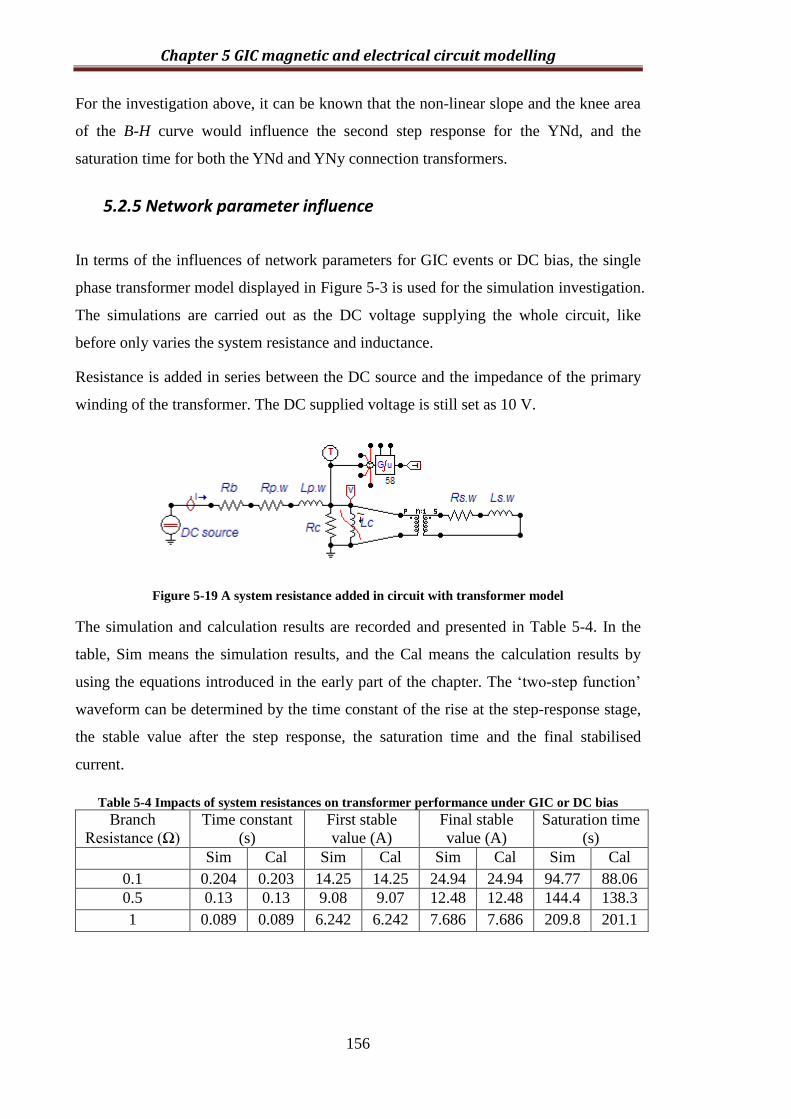
Chapter 5 GIC magnetic and electrical circuit modelling
156
For the investigation above, it can be known that the non-linear slope and the knee area
of the B-H curve would influence the second step response for the YNd, and the
saturation time for both the YNd and YNy connection transformers.
5.2.5 Network parameter influence
In terms of the influences of network parameters for GIC events or DC bias, the single
phase transformer model displayed in Figure 5-3 is used for the simulation investigation.
The simulations are carried out as the DC voltage supplying the whole circuit, like
before only varies the system resistance and inductance.
Resistance is added in series between the DC source and the impedance of the primary
winding of the transformer. The DC supplied voltage is still set as 10 V.
Figure 5-19 A system resistance added in circuit with transformer model
The simulation and calculation results are recorded and presented in Table 5-4. In the
table, Sim means the simulation results, and the Cal means the calculation results by
using the equations introduced in the early part of the chapter. The ‘two-step function’
waveform can be determined by the time constant of the rise at the step-response stage,
the stable value after the step response, the saturation time and the final stabilised
current.
Table 5-4 Impacts of system resistances on transformer performance under GIC or DC bias
Branch
Resistance (Ω)
Time constant
(s)
First stable
value (A)
Final stable
value (A)
Saturation time
(s)
Sim Cal Sim Cal Sim Cal Sim Cal
0.1 0.204 0.203 14.25 14.25 24.94 24.94 94.77 88.06
0.5 0.13 0.13 9.08 9.07 12.48 12.48 144.4 138.3
1 0.089 0.089 6.242 6.242 7.686 7.686 209.8 201.1

Chapter 5 GIC magnetic and electrical circuit modelling
157
As the system resistance is increased, the time constant of the step-response is decreased;
the first stable value of current after the step-response stage; and then the final stable
value of current is decreased as well. Only the saturation time is increased.
Equation (5-8) shows that the time constant is determined by the inductance and
resistance of the system. So the time constant becomes shorter when the branch
resistance is increased. In addition, from (5-9) and (5-10), it can be seen that the primary
side current is determined by the supplied DC voltage level and the total resistance in
the system. When the total resistance in the system is increased, the supplied voltage is
not changed, and then the current must be decreased. The saturation time is mainly
determined by the voltage drop on the core. When adding a resistance connected with
the core in series, then it will re-distribute the ratio of the voltage. The voltage on the
core will be decreased, and then the saturation time will become longer.
Similar to adding system resistance, a system inductance is added in series between the
DC source and the impedance of the primary winding of the transformer. The DC
voltage level is still set as 10 V. A fixed system resistance of 0.5 Ω is connected in order
to accompany the system inductance in the simulation.
Figure 5-20 A system inductance added in circuit with transformer model
Table 5-5 shows the simulation results and calculation results.
Table 5-5 Impacts of system inductances on transformer performance under GIC or DC bias
Branch
Inductance
(mH)
Time constant
(s)
First stable
value (A)
Final stable
value (A)
Saturation time
(s)
Sim Cal Sim Cal Sim Cal Sim Cal
50 0.175 0.175 9.078 9.076 12.48 12.48 144.4 138.3
100 0.221 0.220 9.078 9.076 12.48 12.48 144.4 138.3
200 0.311 0.311 9.078 9.076 12.48 12.48 144.4 138.3
From the results, it can be seen that the system inductance only affects the time constant
of the step response which is mentioned in (5-8).

Chapter 5 GIC magnetic and electrical circuit modelling
158
In the same way as before, with two parameters added to the circuit, the shunt
capacitance is added to the circuit. In the circuit, 0.5 Ω system resistance and 100 mH
system inductance are added at the primary side and a shunt capacitance with a value of
100 µF is added between the system impedance and the winding impedance. The
waveforms of the primary current and flux linkage are displayed in Figure 5-21.
Figure 5-21 Impacts of the shunt capacitance
The overall shapes of the primary current and flux linkage waveform are the same as
those simulated without the shunt capacitance. Even the key features including the step-
response time constant, the step-response stable value, the saturation time and the final
stable value do not change with or without the shunt capacitance. However, the
existence of the shunt capacitance produces some high frequency components due to its
resonance with the system inductance.
5.2.6 Simulation of AC & DC supply
From the last section, it can be seen that the three single-phase transformers bank can be
represented as a single phase transformer in the case of DC supply only. However, a
single-phase model cannot represent three single-phase transformers bank in the AC and
DC mixed supplied situation.
A YNd connected transformer bank is constructed by using a three single-phase
transformer model. There are two sources in the model, one is the AC supplied voltage
at 132 kV and the other is a 10 V DC voltage which is supplied from the neutral of the
primary side Y connection winding to simulate GIC event or DC bias. Large resistances
are connected as load to simulate the no load condition. The simulation model is shown
in Figure 5-22.
Cu
rre
nt(
A)
Time(s)
Flux(W
b)
Cu
rre
nt(
A)

Chapter 5 GIC magnetic and electrical circuit modelling
159
Figure 5-22 Three single-phase transformers bank in YNd connection
System resistance and inductance are set as 1.376 Ohms and 24.968 mH which are
obtained from one of the 132 kV busbar database provided by Electrical Northwest
(ENW).
As mentioned before, the DC voltage supplied to the single phase transformer model is
to simulate the YNd three single-phase transformers bank and results show that the
primary current displays a ‘two-step function’ waveform, which includes the step-
response stage, pseudo-flat stage and the saturation stage. When the DC voltage is
supplied in the neutral of the primary star in the AC powered YNd single-phase
transformers bank, the primary current has the same pattern of waveform, with the
sinusoidal waveform integrated. This is shown in Figure 5-23.

Chapter 5 GIC magnetic and electrical circuit modelling
160
Figure 5-23 Simulation results for Phase A (a): Primary current (b): Step-response of primary
current (c): Magnetising current (d): Current referred from secondary winding
It can be seen that the waveforms are following the supplied AC source, and the
oscillation content in the waveforms is of 50 Hz.
Figure 5-24 compares the saturated part of the primary current, magnetising current and
secondary winding current referred to the primary side. It can be seen that the delta
connected secondary windings influence the primary current because the third order
harmonic current flows into the delta connected loop. Due to the symmetry of the three
phase system, the current of each phase behaves similarly; therefore only phase A is
displayed.
Figure 5-24 Saturated part of primary current, magnetising current and secondary delta connected
winding current referred to primary side
(a) (b)
(c) (d)
Cu
rre
nt(
A)
Time(s)
Cu
rre
nt(
A)
Time(s)
Primary Current
Magnetizing current
Delta winding current referred to primary side
Cu
rre
nt(
A)
Time(s)

Chapter 5 GIC magnetic and electrical circuit modelling
161
At the very beginning, before the core is saturated, as the secondary delta winding
impedance can be seen from the primary side, the magnetising current is relatively small
because of the large core impedance and therefore the primary current is in sine wave.
With the flux accumulating, the core working point goes into the knee region and the
magnetising current roars up to a large value, so does the primary current. Then the core
is saturated and the magnetising current stabilises. At this moment, the primary current
contains bi-polar pulses contributed by the magnetising current and the third harmonic
current from the secondary delta connected windings as shown in Figure 5-24.
When an AC source is present, the saturation time is shortened. Comparing the supplied
DC only case and this case where GIC effects on the AC system are simulated, although
the accumulating speed of the flux remains the same, the additional AC voltage peak
pushes the flux closer to the saturation region, so the time spent on reaching the
saturation is much shorter in the real case of GIC effect.
The AC voltage source also brings the over-current in the saturation stage due to the
saturation of the core. As in the power system, the voltage level of the system is almost
fixed around the rated voltage but the GIC can be varied within a wide range from a few
volts to hundreds of volts, how different levels of GIC affect the value of the stable peak
of the saturation current becomes an interesting and important topic. A series of
simulations have been done to explore the relationship between the DC supply level and
the final stable peak value of the primary current after saturation. The results are shown
in Table 5-6.
Table 5-6 Relationship between the supplied DC level and the final peak current value
Supplied DC voltage (V) 1 5 10 20
Final peak primary current (A) 12.644 46.172 75.387 121.83
Final peak magnetising current (A) 15.198 55.057 89 142.11
Larger DC levels lead to larger final values for the primary current drawn from the
system. Also, the final peak value difference between the primary current and the
magnetising current increases with the DC supply level. This can be explained as the
larger the DC voltage supply, the larger the current will flow in the secondary delta
connected loop.
In reality, a transformer or a system grid is often connected with the load, which is the
function of the grid to transfer the energy. Consequently, whether the load would
influence the GIC effects would become an interesting and important topic to study. RL

Chapter 5 GIC magnetic and electrical circuit modelling
162
loads (with the power factor of 0.8 lagging) are added onto the YNd three single-phase
transformers bank to investigate the effects of load on the GIC effect of transformer
with DC supply at the neutral of the primary-side star connected windings. The
simulation model displayed in Figure 5-22 is used by varying the load. Simulations with
100%, 70%, 50%, 30% and 10% loads respectively are conducted. Key parameters of
the primary current including the stable value of the step response, the saturation time
and the final peak value are recorded which are shown in Table 5-7.
Table 5-7 Load effects on GIC performance of the YNd single phase transformer banks
Load (%)
Stable value
of the step
response (A)
Saturation
time (s)
Saturated magnetising
current peak value (A)
Saturated
primary current
peak value(A)
100 5 59 88.64 184.70
70 5.02 58 88.73 149.03
50 5.02 58 88.70 127.59
30 5.02 57 88.86 107.82
10 5.02 56 88.97 86.14
No load 5.02 55 88.90 75.40
From the data in Table 5-7, the stable current value of the step response is
approximately the same as 5 A, which is independent of the load. Loads have little
influence on the saturation time, although the saturation time increases slightly with the
increase of load. The saturation time is mainly decided by the DC supply level.
The YNy connected three single-phase transformers bank is built for the comparison
with the YNd connection. There are two sources of the model, one is the AC supplied
voltage at 132 kV; and the other is a 10 V DC voltage which is supplied from the
neutral of the primary side Y connection winding to simulate GIC event or DC bias.
Large resistances are connected as load to simulate the no load condition. The
simulation model is shown in Figure 5-25.
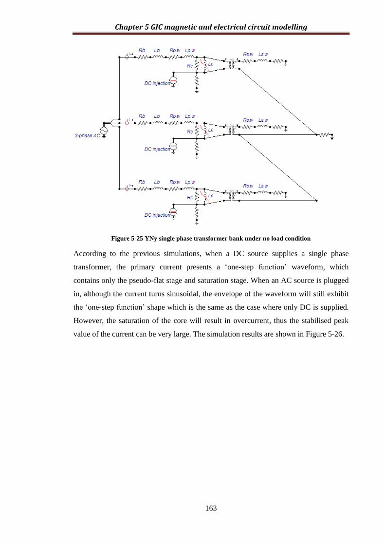
Chapter 5 GIC magnetic and electrical circuit modelling
163
Figure 5-25 YNy single phase transformer bank under no load condition
According to the previous simulations, when a DC source supplies a single phase
transformer, the primary current presents a ‘one-step function’ waveform, which
contains only the pseudo-flat stage and saturation stage. When an AC source is plugged
in, although the current turns sinusoidal, the envelope of the waveform will still exhibit
the ‘one-step function’ shape which is the same as the case where only DC is supplied.
However, the saturation of the core will result in overcurrent, thus the stabilised peak
value of the current can be very large. The simulation results are shown in Figure 5-26.

Chapter 5 GIC magnetic and electrical circuit modelling
164
Figure 5-26 Simulation results for Phase A (a): Primary current (b): Magnetising current (c):
Starting moment (d): Saturation moment
Similar to the case of DC supply only, the primary current presents a ‘one-step function’
envelope. The primary current is comprised of the magnetising current and the current
flowing through the core resistance. At the very beginning, the primary current is so
small and it is a sine wave. With the flux accumulating, the working point of the core
biases and goes into knee area and the magnetising current roars up to a large value, so
does the primary current. Then the core is saturated and the magnetising current is
stabilised.
The saturation time of the primary current is shortened for the case of GIC effect. It is
because the AC peak brings the flux closer to saturation and so less time is needed for
the accumulation of DC flux to bias the working point of the core reach saturation.
Simulations investigating the relationship between the DC levels and the peaks of final
current are performed and the results are shown in Table 5-8.
Table 5-8 Relationship between the supplied DC level and the final peak current value
Supplied DC voltage (V) 1 5 10 20
Final peak primary current (A) 14.79 52.79 86.28 137.64
Final peak magnetising current (A) 14.79 52.79 86.26 137.64
(a) (b)
(c) (d)
Cu
rre
nt(
A)
Time(s)
Cu
rre
nt(
A)
Time(s)

Chapter 5 GIC magnetic and electrical circuit modelling
165
It can be seen that, the stabilised peak value of the primary current is equal to the
saturated magnetising current peak value, which indicates that the primary current peak
values are decided by the magnetising current after saturation. This result is different
from that of the case of the YNd three single-phase transformers bank, since no current
flows in the secondary side. The peak value of the magnetising current increases with
the growth of the supplied DC level, as a larger supplied DC may bring the core into
deeper saturation.
For the load influence, Table 5-9 shows the simulation results by varying the load
percentage. Due to the fact that there is no step-response in the YNy connection, then
there are only three parameters recorded, i.e. saturation time, saturated magnetising
current peak value and saturated primary current peak value.
Table 5-9 Load effects for the YNy single phase transformers bank
Load (%) Saturation
time (s)
Saturated magnetising current
peak value (A)
Saturated primary
current peak value(A)
100 16 84.65 467.19
70 15 84.64 344.78
50 14 85.28 255.58
30 14 85.87 185.72
10 14 84.87 118.61
No load 15 86.23 86.26
Both the saturation time and the magnetising current peak value can be considered to be
independent of the load.
5.3 Case 2: Sensitivity of transformer core structure
In the last section, the influence of the winding connection, core characteristic and
network parameters were discussed by using three single-phase lumped-parameter
transformer models. Supply the DC only and DC mixed with AC are both used for the
simulation studies.
In this section, the influences of core structures or transformer GIC performance will be
discussed which include three-limb and five-limb transformers with the three single-
phase transformers bank acting as the reference.

Chapter 5 GIC magnetic and electrical circuit modelling
166
5.3.1 Comparison between YNd connected three single-phase
transformers bank and three-phase three-limb transformer
As far as the transformer structure is concerned, the main difference between the three
single-phase transformers bank and the three-phase three-limb transformer is that there
is flux coupling among phases by yoke in a three-limb transformer. In addition, there’s
no DC flux passing path in a three-limb transformer.
The simulation was carried out by using the same condition as before which is the
supply DC voltage as 10 V. The comparison of the primary side current waveforms
between a three-limb transformer and three single-phase transformers bank are shown in
Figure 5-27.
Figure 5-27 Comparison between YNd connected 3 single phase transformers bank and three-phase
three-limb transformer
The top figure shows the whole waveforms of primary side current of the two different
core structure transformers; and the bottom two figures show the step-response stage
and the final stage. It can be seen that at the step-response stage and the final stage these
two different core structure transformers have slightly different responses.
Transformers bank
3-leg transformerCu
rre
nt(
A)
Time(s)
Cu
rre
nt(
A)
Cu
rre
nt(
A)
Time(s)

Chapter 5 GIC magnetic and electrical circuit modelling
167
Table 5-10 shows the key parameters of the comparison between the transformers bank
and the three-phase three-limb transformer.
Table 5-10 Comparison between YNd connected transformers bank and three-phase three-limb
transformer
Parameters Time
Constant (s)
Stable value of
the step response
(A)
Saturation
Time (s)
Saturated
primary current
peak value(A)
Phases A B C A B C A B C A B C
Transformers
bank 0.24 0.24 0.24 16.6 16.6 16.6 32 32 32 259 259 259
Three-limb
transformer 0.15 0.15 0.15 20.2 20.2 20.2 75 75 75 220 220 220
It can be seen from Figure 5-27 and Table 5-10, the time constant of the step-response
part is different; the three-phase transformer has a shorter time constant, a higher stable
value of current of the step-response; also the saturation time is longer; and the final
current value is higher than the three single-phase transformers bank.
The zero sequence core impedances of the two transformers are different, and the zero
sequence core impedance is connected in parallel with the positive sequence core
impedance and the impedance of secondary delta connected windings. The system
equivalent resistance and inductance at the step response stage and pseudo flat stage is
decreased; as a result, in the case of three-limb transformer, the step response stable
value is increased and the time constant of the step response is decreased.
As far as the magnetic field is concerned, in the three single-phase transformers bank,
each phase has its own core which has high permeability and provides low reluctance
path for the flux passing through, including positive, negative and zero sequence flux.
Thus there is no flux coupling among phases, the magnetic flux of each single phase
transformer is considered to be inside the core only. However, for the three-phase three-
limb transformer, there is no low reluctance path for DC flux to pass, the only way for
the DC flux to pass through is to leak out of the core and go through the winding, oil,
tank and so on. However, those materials have low permeability and thus high
reluctance.
When the same level of DC voltage is supplied into the transformer via neutral, the high
reluctance loop is harder for the DC flux to be accumulated in the transformer core; then
it is harder for the three-limb transformer to be saturated therefore the three single-phase
transformers bank.
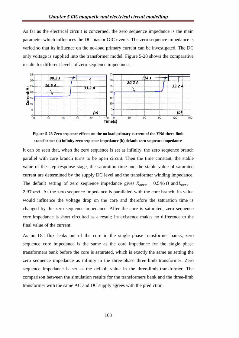
Chapter 5 GIC magnetic and electrical circuit modelling
168
As far as the electrical circuit is concerned, the zero sequence impedance is the main
parameter which influences the DC bias or GIC events. The zero sequence impedance is
varied so that its influence on the no-load primary current can be investigated. The DC
only voltage is supplied into the transformer model. Figure 5-28 shows the comparative
results for different levels of zero-sequence impedances.
Figure 5-28 Zero sequence effects on the no load primary current of the YNd three-limb
transformer (a) infinity zero sequence impedance (b) default zero sequence impedance
It can be seen that, when the zero sequence is set as infinity, the zero sequence branch
parallel with core branch turns to be open circuit. Then the time constant, the stable
value of the step response stage, the saturation time and the stable value of saturated
current are determined by the supply DC level and the transformer winding impedance.
The default setting of zero sequence impedance gives and
. As the zero sequence impedance is paralleled with the core branch, its value
would influence the voltage drop on the core and therefore the saturation time is
changed by the zero sequence impedance. After the core is saturated, zero sequence
core impedance is short circuited as a result; its existence makes no difference to the
final value of the current.
As no DC flux leaks out of the core in the single phase transformer banks, zero
sequence core impedance is the same as the core impedance for the single phase
transformers bank before the core is saturated, which is exactly the same as setting the
zero sequence impedance as infinity in the three-phase three-limb transformer. Zero
sequence impedance is set as the default value in the three-limb transformer. The
comparison between the simulation results for the transformers bank and the three-limb
transformer with the same AC and DC supply agrees with the prediction.
Cu
rre
nt(
A) 16.6 A
20.2 A33.2 A 33.2 A
88.2 s 114 s
Time(s)
(a) (b)

Chapter 5 GIC magnetic and electrical circuit modelling
169
5.3.2 Comparison between YNy connected three single-phase
transformers bank and three-phase three-limb transformer
The same simulation investigation is carried out on the YNy connected transformer
model. Figure 5-29 shows the comparison results between the transformer banks and the
three-limb transformer. The Y-axis on the left side is for the transformer banks; and the
Y-axis on the right side is for the three-limb transformer.
Figure 5-29 Comparison between YNy connected 3 single phase transformers bank and three-phase
three-limb transformer
It can be seen that a ‘one-step function’ waveform occurs for the primary current of the
transformer banks, while the current of three-limb transformer has a ‘two-step function’
waveform due to the zero sequence core impedance in parallel with the transformer core.
The current rises much sooner for the transformers bank because more DC voltage
would be dropped on the core which means the accumulating speed of the flux is higher
than that in the three-limb transformer. The stable step response current value for the
three-limb transformer is 11.7 A. Table 5-11 shows almost all of the key parameter
values.
Transformers bank
3-leg transformer
Cu
rre
nt(
A)
Time(s)
Cu
rre
nt(
A)
Time(s)
Cu
rre
nt(
A)

Chapter 5 GIC magnetic and electrical circuit modelling
170
Table 5-11 Comparison between YNd connected transformers bank and three-phase three-limb
transformer
Parameters Time
Constant (s)
Stable value of
the step response
(A)
Saturation
Time (s)
Saturated
primary current
peak value(A)
Phases A B C A B C A B C A B C
Transformer
bank / / / / / / 16 16 16 286 286 286
Three-limb
transformer 0.15 0.15 0.15 11.7 11.7 11.7 55 55 55 176 176 176
It can be seen that both of the two transformers under YNy connection are saturated
earlier as compared with the YNd connection.
To understand the influence of the zero sequence core impedance in the YNy three-limb
transformer, the DC only voltage is supplied and the zero sequence core impedances of
the transformer are varied. The simulation results are shown in Figure 5-30.
Figure 5-30 Zero sequence effects on the no load primary current of the YNy three-phase three-
limb transformer (a) infinity zero sequence impedance (b) zero sequence impedance between
infinity and default value (c) default zero sequence impedance
It can be seen that the step response stage cannot be observed as the time constant turns
to be infinity when zero sequence core impedance is set as infinity, due to the fact that
the transformer core impedance is in series with the primary winding impedance in the
circuit. The pseudo-flat stage and the saturation stage still exist and the saturation time
and the final current value can be calculated.
33.2 A
45 s
33.2 A
60 s
33.2 A
70 s
(a) (b)
(c)
Cu
rre
nt(
A)
Time(s)
Cu
rre
nt(
A)
Time(s)

Chapter 5 GIC magnetic and electrical circuit modelling
171
With the zero sequence core impedance is decreased from the infinity to a definite value,
the time constant of the step response stage gradually drops, thus the beginning part of
the waveform of the primary current rises gradually as shown in Figure 5-30 (b). And
the waveform is similar to one of the experimental results published by P.Price [70].
Decreasing the zero sequence core impedance down to the default value, the simulation
results are shown in Figure 5-30 (c). The ‘two-step function’ waveform is shown again.
As the zero sequence core impedance is decreased, the saturation time is increased.
5.3.3 Five-limb transformer
The five-limb transformer core is different from the three-limb transformer core and the
single phase transformer core as well. First, there is a loop on the core for DC flux
passing through which is similar to the single phase transformer core; second, there is
coupling among phases via the yoke of core which is similar to the three-limb
transformer core. So the five-limb transformer has some combined features of the other
two transformer core structures.
The response of the five-limb transformer to GIC is investigated in the following by
using one of several existing transformers working in the National Grid network. The
transformer is a 400/275/13 kV, 1000 MVA, YNad winding connection. Table 5-12
shows the basic information of the transformer model applied in this simulation.
Table 5-12 Basic information and test data of the three-phase five-limb transformer
Short Circuit Test Data Open Circuit Test Data
Voltage
Level Power Base
Impedance
(%)
Losses
(kW)
No Load
Voltage
(%)
Average
Current
(A)
No Load
Losses
(kW)
Primary:
400 kV
HV/LV
@1000MVA 16.78 1383 90 6.177 96.3
Secondary:
275kV
HV/T
@60MVA 7.29 71.9 100 13.15 127.9
Tertiary:
13kV
LV/T
@60MVA 5.97 77.3 110 55.433 175.3
In accordance with the test data and the basic information, a five-limb hybrid
transformer model is built for the simulation studies. In the circuit, there is a three-phase
400 kV AC source connected with the transformer and 100 V DC voltage supplied from
the neutral point of the primary side star connected windings into the transformer. No
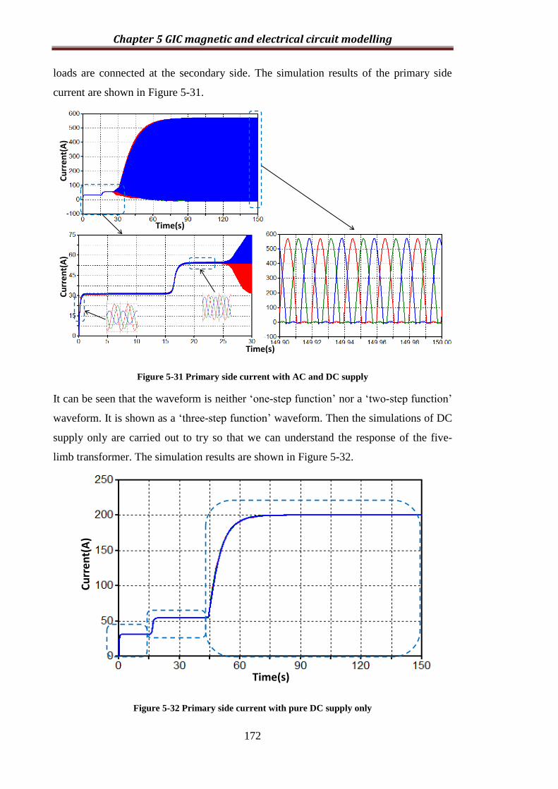
Chapter 5 GIC magnetic and electrical circuit modelling
172
loads are connected at the secondary side. The simulation results of the primary side
current are shown in Figure 5-31.
Figure 5-31 Primary side current with AC and DC supply
It can be seen that the waveform is neither ‘one-step function’ nor a ‘two-step function’
waveform. It is shown as a ‘three-step function’ waveform. Then the simulations of DC
supply only are carried out to try so that we can understand the response of the five-
limb transformer. The simulation results are shown in Figure 5-32.
Figure 5-32 Primary side current with pure DC supply only
Cu
rre
nt(
A)
Time(s)
Cu
rre
nt(
A)
Time(s)
Cu
rre
nt(
A)
Time(s)

Chapter 5 GIC magnetic and electrical circuit modelling
173
It can be seen that the primary side current is a ‘three-step function’ waveform. For the
first two steps, their flat parts are not truly flat, since the current still actually increases
but in a very slow slope. For the last step, the current is finally stabilised and is
maintained at the same level.
Compared with the ‘two-step function’ waveform of the primary side current of the
YNd connected three-limb transformer, the ‘three-step function’ waveform of the YNad
five-limb transformer has an extra step, and this is because the extra component forms
the core structure, the side yoke.
For the first step, it is as the same as the step-response controlled by delta winding, as
was previously explained. However, in this step, the DC flux accumulates inside the
core through the side yoke, which then has a different reluctance from the positive
sequence core reluctance.
For the second step, the whole DC flux continues to accumulate and flow through the
side yoke, until the side yoke is saturated. The saturation of the side yoke causes the
second rise of the primary current. After the side yoke is saturated, the DC flux cannot
be absorbed any more into the side yoke so the only way for them is to leak out of the
core and go into the oil and tank. In other words, the five-limb transformer tends to
become a three-limb transformer after the side yoke is saturated.
For the last step, DC flux further increases in the transformer core; the entire core goes
into saturation. Then the total non-linear core inductance starts to decrease and the
primary side current rises swiftly, which can be observed as the rise in the third step.
After the entire core is fully saturated, the core inductance drops to a very small value
which indicates that the short circuit and primary side current are finally stabilised.
All the key parameters can be calculated by using the same method as previously done
in this chapter. The calculation results are shown in Table 5-13.
Table 5-13 Key parameters of the primary side current with pure DC voltage supply
31.3 A 54.3 A 200.78 A 0.195s 15.6s 44s 90s
: The time constant of the step response
: The time instant when the second rise starts
: The time instant when the third rise starts
: The time instant when the entire core is fully saturated
: The stable value of the step response
: The stable value after the side yoke is saturated
: The stable value after the entire core is fully saturated

Chapter 5 GIC magnetic and electrical circuit modelling
174
Compared with the simulation results, the calculated , and match the simulation
results very well; this verifies the explanation of the ‘three-step function’ waveform of
the primary side current with pure DC voltage only for the three-winding YNad five-
limb transformer. The explanation is also suitable for the case of AC supply and
Supplied DC as well. The waveform still follows the ‘three-step function’ as shown in
Figure 5-31. The key parameters of the primary side current waveform are shown in
Table 5-14.
Table 5-14 Key parameters of the primary side current with AC&DC voltage supplied
(A) (A) (A) (s) (s) (s) (s)
Phase A 31.3 54.3 571.79 0.195 15.6 25.6 78
Phase B 31.3 54.3 571.79 0.195 15.6 25.6 78
Phase C 31.3 54.3 571.79 0.195 15.6 25.6 78
, , , , , , symbols follow the definition as in Table 5-13. Ipeak is the
stable peak value after the entire core is fully saturated. and values are the RMS
value in this table. Compared with the case of DC supply only, , , and have
the same values as the DC level remains the same. It reflects that those parameters are
really determined by the DC supply level in the five-limb transformer core. , and
are determined by both of the levels of AC and DC supply.
5.3.3.1 Winding connection
As we know, winding connections have several common types used for power
transformers. There are two windings and three windings connection transformers. The
original transformer used in the simulation is the YNad connection transformer. The
investigation is carried out by varying the winding connection types which include
YNyd (three-winding connection), YNy (two-winding) and YNd (two-winding). All
other configurations remain the same, e. g. voltage level, power rating, short circuit test
data, open circuit data and core structure. Pure DC voltage source is supplied in this
simulation.
Figure 5-33 shows the primary side current waveform for three types of connection. It
can be seen that the ‘three-step function’ waveform is shown for the Yyd and YNd
connection, except the YNy connection. The waveform of the YNy connection is only a
‘two-step function’; since there is no secondary side delta connected winding in the
circuit in YNy connection. Therefore, the transformer core impedance needs to be taken

Chapter 5 GIC magnetic and electrical circuit modelling
175
into account from the beginning; it increases the time constant of the step-response then
causes the current value to keep a low value. It also shortens the time allowed for
saturation. In addition, the final saturated stable value of the current is the lowest in the
Yyd connection due to the extra winding impedance.
Figure 5-33 Primary side current of Yyd, YNd and YNy connection transformer
Comparing all the four types of winding connection, the final saturated current value of
the YNad connected transformer is the lowest one, and the saturation time is the longest
one. Table 5-15 shows the key parameters of the primary currents for all the four types
of transformer winding connection.
Table 5-15 Simulation results for the primary side current in all four type of connection
(A) (A) (A) (s) (s) (s) (s)
YNad 31.3 54.3 200.8 0.195 15.6 44 90
Yyd 29.3 212.4 433.6 0.18 4.5 17 36
Yd 45.2 530.8 903.8 0.39 8.1 23.8 70
Yy / 270 903.8 / 4.2 13.3 44
‘Three-step function’ waveform still appears on the YNd connected transformer; while
the primary side current of the YNy connected five-limb transformer has a ‘two-step
function’ waveform. The first step response is missing in the YNy connection, also in
the YNd connection, the stable value of the step response is half the final stable value.
Yyd connection
YNd connection YNy connection
Cu
rre
nt(
A)
Time(s)
Cu
rre
nt(
A)
Time(s)

Chapter 5 GIC magnetic and electrical circuit modelling
176
In these YNd and YNy connected cases, the winding impedance is identical, the only
difference is that the secondary winding impedance cannot be seen from the primary
side when it is open circuited in the YNy connection; on the other hand it can be seen in
the YNd connection due to the zero sequence component loop provided by the delta
winding. The final values of the current are the same in both YNd and YNy connections
as it is decided by the DC voltage level and the primary winding resistance.
5.3.3.2 Five-limb area ratio influence
It can be seen that the ratio of the side yoke and main yoke would influence the flux
distribution of the five-limb transformer core at the steady state which is mentioned in
Chapter 4. In this section, the transient influence of the area-ratio on GIC performance
will be discussed.
The simulation was carried out by varying the ratio of the main yoke area and the side
yoke area from 0.7/0.3 to 0.5/0.5, each 0.05 as a step and using the original connection
of YNad as the transformer winding connection. The DC supply voltage is fixed as 100
V to investigate the different reactions for different area ratio. The simulation results are
shown in Table 5-16.
Table 5-16 Simulation results for main-side yoke area ratio modified
Area Ratio
Main /Side yoke (A)
(A)
(A)
(s)
(s)
(s)
(s) A B C
0.7/0.3 31.3 40.3 200.78 0.195 7.1 40 130 130 130
0.65/0.35 31.3 40.3 200.78 0.195 8.9 40 130 130 130
0.6/0.4 31.3 39.7 200.78 0.195 9.9 40 130 130 130
0.55/0.45 31.3 38.7 200.78 0.195 10.7 40 140 140 140
0.5/0.5 31.3 37 200.78 0.195 12.5 40 165 165 165
It can be seen that by reducing the main yoke area and side yoke area ratio to the area of
the core limb, the side yoke becomes easier to saturate; thus the second rise of the
primary side current comes earlier. In addition, the final saturation time is also reduced.
Since the modification to the side yoke area may also affect the λ-I curve of each part of
the core, the third step of the ‘three-step function’ waveform may be changed. The
simulation results of the primary current waveforms are shown in Figure 5-34.

Chapter 5 GIC magnetic and electrical circuit modelling
177
Figure 5-34 Primary side current waveform with main-side yoke area ratio modified
It can be seen that the ‘three-step function’ waveform remains. Modifying the areas of
the main yoke and side yoke has no impact on the primary side current of step-response
and the final stabilised current value. They are decided by the DC voltage level and the
transformer winding impedance.
However, as mentioned before, reducing the side yoke area, would make it easier for the
side yoke to be saturated, the second rise of the primary side current waveform would
come earlier which is shown in Figure 5-34.
Meanwhile, the zero sequence core impedance, which is parallel with the delta
connected tertiary winding impedance, is increased; therefore the stable current value
after the saturation of the side yoke is decreased since the overall resistance is increased.
Figure 5-35 shows the side yoke and main limb λ-I curves with different main yoke/side
yoke area ratio.
Figure 5-35 Side yoke and main limb λ-I curves with different main-side yoke area ratio
Cu
rre
nt(
A)
Time(s)
Flu
x(W
b)
Current(A)
Outer leg λ-I curve Inner leg λ-I curve

Chapter 5 GIC magnetic and electrical circuit modelling
178
It can be seen that the change of the ratio of the main yoke and side yoke area would
influence both of the side yoke and main limb λ-I curves. The left side figure represents
the side yoke characteristics and the right side figure represents the main limb
characteristic. As a result, the saturation characteristics would be changed as well. It
would bring the difference to the second and third step waveforms. In addition,
significant change on the main limb λ-I curve is observed when the main yoke/side yoke
area ratio changes from 0.55/0.45 to 0.5/0.5. From the right side of the figure, it can be
seen that, when it is further reduced, the maximum flux of the main limb increases and
the knee area gets smoother and smoother. This is why the saturation time increases and
the third rise of the waveform does not appear that steep.
5.3.3.3 Effects of the system impedance R & L
Since the ‘three-step function’ waveform of the five-limb transformer is different from
the other two types of transformer core structures, the system R and L are added at the
primary side of the transformer so that the influence on the primary current or
magnetising current of the transformer can be investigated. The simulation was carried
out by only supplying 100 V DC voltage; no load is connected to the transformer, the
primary side current is observed to investigate the effects of additional system R and L.
The simulation was carried out by discussing the influence of the resistance and
inductance separately. The first step is to vary the resistance value from 0.5 Ohm, 1
Ohm to 2 Ohm, and then the second step is to fix the resistance value as 0.5 Ohm and to
vary the inductance value from 100 mH, 200 mH to 400 mH. The key parameter values
of the simulation results are shown in Table 5-17 and Table 5-18.
Table 5-17 Simulation results for the key parameters by varying system R
R (Ω) (A) (A) (A) (s) (s) (s) (s) 0.5 27 42.8 100.2 0.17 18 54 93
1 23.9 35.3 66.75 0.15 20.5 64.3 98
2 19.3 26 40 0.12 25.1 83.8 103
It can be seen that when the total primary side resistance is increased, the time constant
of the step-response, the stable value after the step response and the final stable value of
the ‘three-step function’ primary side current waveform are decreased. In addition,
because of the growth of the equivalent primary side resistance, the DC voltage
dropping on the core would be decreased, and then the DC flux would accumulate more
slowly and would take more time for the side yoke and the entire core to saturate. As a

Chapter 5 GIC magnetic and electrical circuit modelling
179
result, the time taken for the second and third rise to occur is lengthened and the total
saturation time for the entire core is longer.
Table 5-18 Simulation results for the key parameters by varying system L
L(mH) (A) (A) (A) (s) (s) (s) (s)
100 27 42.8 100.2 0.197 18 54 93
200 27 42.8 100.2 0.22 18 54 93
400 27 42.8 100.2 0.27 18 54 93
It can be seen that by varying the system L it would only influence the time constant of
the step response. The time constant of the step-response is increased with the increase
of the system L value, and the slower rising speed of the current after the DC supply is
seen.
5.4 Summary
In this chapter, the transformer core structure influence on the primary current or
magnetising current under the DC bias or GIC events has been successfully identified
by using simulation case studies. Based on the results analysis of the simulation cases,
the effects of the winding connection, the core structure, and the network parameters on
the magnetising currents of the transformers can be summarised as follows:
1. For the waveform of the primary side of the current, its step times are influenced
by the winding connection, the core structure and the zero sequence core
impedance. In short, the ‘one-step function’ waveform only appears for a single
phase transformer with the YNy winding connection; the ‘two-step function’
waveform appears for a single phase transformer and a three-limb transformer
and a five-limb transformer with a YNd winding connection; the ‘three-step
function’ waveform appears for a five-limb transformer with three windings
YNad or two windings YNd connection.
2. The three stages are defined in a ‘two-step function’ waveform, which are the
step-response stage, the pseudo-flat stage and the saturation stage. The step-
response stage only appears when there is low value impedance connected in
parallel with the core impedance in the equivalent circuit. The durations of the
pseudo-flat stage and the final saturation are controlled by the accumulating
speed of the zero sequence DC flux which the DC voltage dropped on the core.

Chapter 5 GIC magnetic and electrical circuit modelling
180
3. Transformer winding impedance controls the behaviour of the primary side
current. Winding impedance combined with DC supply level decides the time
constant and the stable value of the step response. The system impedance gives
the same effect as the winding impedance. Core saturation characteristics mainly
control the saturation stage, including the speed of the rise and the time for the
saturation.
4. The zero sequence impedance of the three-phase three-limb transformer is more
complex than that of the three single-phase transformers bank. In a three-limb
transformer, DC flux cannot find a return path inside of the core and has to leak
out of the core and circulate through the oil and tank. The zero sequence
impedance in the three-limb transformer affects the step response time constant
and the stable value and also it impacts the saturation time by influencing the
DC voltage drop on the transformer core. The experiments done by Tokyo
Electrical Power show the same pattern as the simulation results in this chapter
hence it confirms the above conclusion. [71]
5. Three-step waveform appears on the primary side current of the five-limb
transformer. The cause of the first step function is the same as explained before
the step response, the second step function is due to the saturation of side yoke,
and the third step function is caused by the saturation of the entire core.
6. Reducing the side yoke area ratio makes the side yoke easier to saturate in a
five-limb transformer. As a result, the second rise in the three-step function
waveform becomes earlier and the stable value of the current is decreased.
Modifying the side yoke area ratio also has some impact on the third rise of the
waveform.
7. R, L loads connected at the secondary winding side have no influence on the
severity of the GIC response of the transformers.
Chapter 6 Low frequency switching transient magnetic and electrical modelling
181
Chapter 6 Low frequency switching
transient magnetic and electrical
modelling
6.1 Introduction
In Chapter 5, the DC bias or GIC event has been simulated by using ATP/EMTP
software; and the results have been discussed. All the parameters in the circuit have
been examined including the network parameters, the winding connection and the core
structure of transformer.
In the UK distribution networks, a grid transformer tends to be operated by the circuit
breaker in the upstream substation and a fair length of cable or overhead line is
connected in between the upstream and the downstream substations. De-energising a
transformer with a long cable connected to it can induce the occurrence of ferroresonant
transients due to the interaction between the cable and the transformer.
In this chapter, one of the low frequency transients will be discussed and the effects of
parameters in circuit will be studied via ATP/EMTP simulation. Normally, the low
frequency phenomena include inrush and ferroresonance as mentioned in the literature
review; only the ferroresonant transient phenomenon associated with de-energisation
operation in a UK distribution network will be investigated.
6.2 Distribution network layout
In the UK, when the network was initially built in the 1960s, the cost of the circuit
breaker was exceedingly high; and to save the capital cost of the power system network,
a typical network is configured in such a way that a grid transformer in the downstream
substation is to be operated by the circuit breaker in the upstream substation via a fair
length of cable or overhead line. The typical network is shown in Figure 6-1.

Chapter 6 Low frequency switching transient magnetic and electrical modelling
182
Upstream
Substation
Busbar
Upstream Circuit
Breaker
Long Distance
Cable/Overhead
Line
Disconnector
Grid
Transformer
VT
Downstream
Busbar
Grounding
Transformer
Short
Distance
Cable
Downstream Circuit
Breaker
Figure 6-1 Typical UK distribution network diagram
However, this kind of circuit configuration would usually be susceptible to
ferroresonance occurrence, during the switching operations in distribution networks.
When maintenance, system re-configuration or fault clearance on the network is needed,
switching operations are carried out; switching a transformer with a long cable
connected to it can be problematic due to the interaction between the cable capacitance
and the transformer non-linear core; upon de-energising operations switching
ferroresonant transients would occur. This type of transient was not specified in
standard factory tests and therefore transformers cannot be tested before acceptance and
commissioning. Depending on individual transformer design, some transformers may be
able to withstand the ferroresonant transient and the associated energy dumped into
them without causing localised overheating, whereas the others might not. [45]
It is therefore of interests for a utility to understand the causes, the impacts and the
mitigation measures of switching ferroresonant transients when de-energising a
transformer, in order to maintain failure-free network operations or at least with a
minimum rate of failure.
The utility of Electricity North West first noticed the ferroresonant transients when de-
energising one of the transformers in Preston East Substation during a system
reinforcement project. During commissioning Preston East substation, a so called
'switching transient ferroresonance' problem was experienced when de-energising two
132/33 kV, 45/90 MVA grid transformers. The transformers are configured to be
energised /de-energised by circuit breakers at Penwortham East substation via 11.5 km
long 132 kV polymeric cables and an audible "clunk" noise can be heard from one of
the transformers when it was de-energised.
The same phenomenon happened on the Bloom Street Substation as well. This
confirmed that ferroresonant transients are commonly associated with transformers in
such a network configuration. Field experimental investigations were carried out, as

Chapter 6 Low frequency switching transient magnetic and electrical modelling
183
well as recording voltage and current waveforms, acoustic sensors designed for partial
discharge detection and location were used to pick up the audible noise in an attempt to
pin-point the source location. During this investigative field test oil samples were taken
before and after the tests for DGA analysis [12].
6.3 Case 1: Bloom street substation circuit
6.3.1 Introduction of the circuit
There are two transformers--GT1 and GT2 at Bloom Street Substation (BSS) which the
layout of which is shown in Figure 6-2. Both are 132/33 kV, 45/90 MVA, 3 phases 50
Hz, ONAN/OFAF, YNd1 connection, transformers made by GEC Alstom Stafford in
1997 and installed in 1999. The upstream substation is South Manchester Substation
(SMS); the 132 kV circuit breakers (CB) are installed in SMS and between SMS and
BSS there are 9.5 km single-core XLPE cables connecting the transformers and circuit
breakers. The red circles mark the circuit under study in Figure 6-2, which includes the
CB and 132kV XLPE cable going out from SMS to BSS.
Figure 6-2 South Manchester Substation (SMS) and Bloom Street Substation (BSS) layout
The relevant part of distribution network for de-energising a 132/33kV grid transformer
includes: in the upstream substation busbar, circuit breaker, isolator and the cable and in
9.5 km single-core XLPE cables
Bloom Street Substation (BSS)South Manchester Substation (SMS)
Ground

Chapter 6 Low frequency switching transient magnetic and electrical modelling
184
the downstream substation isolator, grid transformer, auxiliary transformer, a short
length cable, voltage transformer and circuit breaker. The circuit arrangement is given
in Figure 6-3.
Figure 6-3 Single line diagram of the circuit
6.3.2 Recorded transformer de-energisation voltage and current data
The voltages and currents of the transformer were recorded via the protection VTs and
CTs using a transient recorder, when the tests were carried out in Bloom Street
Substation. The three-phase 132 kV line currents and 33 kV line voltages were recorded.
The transient recorder has a sampling frequency fs = 12.8 kS/s which means that each
cycle of the power frequency contains 256 sampling points.
After de-energisation, the transformer voltage and current waveforms recorded were
seen as oscillatory and transient in nature. The whole transient process lasts for less than
0.62 s. The voltage has a square like waveform, and the current oscillates between
positive and negative spiky high magnitudes.
6.3.2.1 Type 1---Results of GT1 first switch-off operation
The 33 kV CB was first opened to shed the load and after one to two minutes the 132
kV CB was opened to de-energise the no-load grid transformer, GT1. To aid
comparisons among all the voltage and current waveforms, the same number of 50 Hz
cycles prior to the voltage change is taken for plotting in all figures.
Figure 6-4 shows the three line voltages at the 33 kV side of the transformer which are
in phase with 132 kV side phase voltages (A phase, B phase and C phase). The whole
process of switching ferroresonant transients lasts for less than 1 s.
BSSSMS
AUX T2
Grid Transformer T2

Chapter 6 Low frequency switching transient magnetic and electrical modelling
185
0.5 0.6 0.7 0.8 0.9 1.0 1.1 1.2 1.3 1.4 1.5-5x10
4
-4x10⁴
-3x10⁴
-2x10⁴
-1x10⁴
0
1x10⁴
2x10⁴
3x10⁴
4x10⁴
5x10⁴
Vo
lta
ge
(V
)
Time (s)
A-B Voltage
B-C Voltage
C-A Voltage
Figure 6-4 Line voltages at transformer 33 kV terminals
It can be seen that Figure 6-4 shows voltage waveforms change from a sin wave to a
square wave after the CB is opened; the voltage waveform levels off as dc-like for 2-3
ms and due to flux linkage which is the integral of voltage by time, the flux linkage
increases to the level of saturation, owing to the non-linear inductance characteristics of
the core inductance would become small at the saturation region and the dc-like voltage
will drop quickly to zero and then go to negative, the core reverses to the linear region
and the voltage waveform levels off dc-like for some more milliseconds. It also shows
that all three-phase voltages decay within a short time period around 0.62 s. Given the
equivalent capacitance of the 9.5 km cable is 1.096 uF (see appendix) and the time
constant for paralleled resistance and capacitance is given as RC , the estimated
resistance value of the parallel resistor is around 100 kOhms.
Figure 6-5 shows the 3-phase line currents at transformer 132 kV side. It shows that
after CB opening the currents of three phases oscillate between positive and negative
polarities and high magnitude spiky currents occur simultaneously with the rapid
change of voltage polarities. When the core of the grid transformer works at the
saturation region the currents suddenly increase in magnitude. Overall the currents also
gradually decay due to the effect of resistive loss.

Chapter 6 Low frequency switching transient magnetic and electrical modelling
186
0.5 0.6 0.7 0.8 0.9 1.0 1.1 1.2 1.3 1.4 1.5
-150
-100
-50
0
50
100
150
Cu
rre
nt
(A)
Time (s)
Phase A
Phase B
Phase C
Figure 6-5 Line currents at transformer 132 kV terminals
Figure 6-6 and Figure 6-7 focus further on the short initiation period of ferroresonant
transients and plot three-phase voltages and three-phase currents. On the current and
voltage waveforms around t = 0.60 s, the changes of currents and voltages seem to
happening simultaneously. Some high frequency components on the voltage waveforms
near to t = 0.60 s can be vaguely seen and since the voltage waveforms were measured
at the 33 kV side, and high frequencies are not easily transferred between HV and LV
windings, this indicates that high frequency oscillations with stronger magnitudes may
exist at 132 kV side phase voltages.

Chapter 6 Low frequency switching transient magnetic and electrical modelling
187
Figure 6-6 Line voltages at transformer 33 kV terminals – zoomed waveforms for 40 ms
In Figure 6-6 when three-phase voltages are distorted from sin waves, they stay flat for
around 3 ms before changing simultaneously. The yellow (green line) phase is near to
the positive peak when ferroresonance occurs and the other two phases, red and blue are
at/near to the half magnitude of the negative peak. When the voltages are in the rapid
changing region, there are five gradients of slopes which can be seen in Figure 6-6 by
circles. Since the voltage rapid changing region is the time when the core goes into
saturation, the gradients mean that the core works at different parts of the B-H curve of
the core.
Figure 6-7 shows that before CB opening the current measured at the 132 kV side are
magnetising currents with magnitude near to zero, not measurable by the protection CTs.
After CB opening the currents of three-phase increase at the same time and with the
same magnitude: the peak values are around 10 A and the frequencies are around 400
Hz, at or near to the time t =0.60 s. They behaved like zero sequence currents since
secondary windings are delta connected. The large magnitude ferroresonant currents
then follow and they start to move to different polarities for three phases. The currents
take complicated patterns. It is assumed that this is due to mixing the components of
zero sequence current and high magnitude spiky ferroresonant current. On each phase
the maximum value of current can reach 90 A.
0.584 0.588 0.592 0.596 0.600 0.604 0.608 0.612 0.616 0.620 0.624-5x10
4
-4x10⁴
-3x10⁴
-2x10⁴
-1x10⁴
0
1x10⁴
2x10⁴
3x10⁴
4x10⁴
5x10⁴
Vo
lta
ge
(V
)
Time (s)
A-B Voltage
B-C Voltage
C-A Voltage

Chapter 6 Low frequency switching transient magnetic and electrical modelling
188
0.584 0.588 0.592 0.596 0.600 0.604 0.608 0.612 0.616 0.620 0.624
-150
-100
-50
0
50
100
150
Cu
rre
nt
(A)
Time (s)
Phase A
Phase B
Phase C
Figure 6-7 Currents at transformer 132kV terminals – zoomed waveforms for 40 ms
Figure 6-8 shows the voltages/currents of the transformer plotted in the same graph. The
corresponding relationship between the current and voltage waveforms is shown: a
higher magnitude current corresponds to the rapidly changing voltage; and the flat dc-
like voltage corresponds with the zero sequence current.
0.584 0.588 0.592 0.596 0.600 0.604 0.608 0.612 0.616 0.620 0.624
-5x10⁴
-4x10⁴
-3x10⁴
-2x10⁴
-1x10⁴
0
1x10⁴
2x10⁴
3x10⁴
4x10⁴
5x10⁴
A-B Voltage
B-C Voltage
C-A Voltage
Vo
lta
ge
(V
)
Time (s)
-150
-100
-50
0
50
100
150
Phase A
Phase B
Phase C
Cu
rre
nt
(A)
Figure 6-8 Voltages/currents of the transformer near to the initiation of ferroresonance

Chapter 6 Low frequency switching transient magnetic and electrical modelling
189
Figure 6-9 Voltages/integrated fluxes of the transformer
Figure 6-9 shows the relationship between the flux leakage in the core limb by
integrating the 33 kV line voltage with the time and voltage of the 33 kV winding.
When the transformer works at a steady state the flux is a pure sin wave. However after
the CB is opened, the flux waveform is distorted and becomes larger than the maximum
value of the steady state flux. This means that, after the switching operation, the core
limb goes into saturation. The plotted flux linkage indicates that each limb will take its
turn to go into saturation.
6.3.2.2 Type 2---Results of GT2 second switch-off operation
The second type of ferroresonant voltage and current waveforms was obtained during
the second switching operation of GT2. The ferroresonance voltages and currents last
for less than 1 s, in the same way as type one before they are completely decayed to
zero; the ferroresonant voltage is in the shape of a square wave and the ferroresonant
current oscillates between positive and negative polarities with high spiky during the
core saturation. Three ferroresonant currents are all in similar shapes and their
magnitudes follow 1:-0.5:-0.5 proportionate to one another. The maximum magnitude
of the three-phase currents can be achieved around 130 A.
Figure 6-10 shows the three-phase voltages near to the initiation of ferroresonance. In
this case, the blue phase voltage is near to the negative peak value when ferroresonance
0.58 0.59 0.60 0.61 0.62 0.63 0.64-5x10
4
-4x10⁴
-3x10⁴
-2x10⁴
-1x10⁴
0
1x10⁴
2x10⁴
3x10⁴
4x10⁴
5x10⁴
Vo
lta
ge
(V
)
Time (s)
A-B Voltage
B-C Voltage
C-A Voltage
-4.0x10⁶
-2.0x10⁶
0.0
2.0x10⁶
4.0x10⁶
A-B Flux
B-C Flux
C-A Flux
Flu
x (
Wb
)

Chapter 6 Low frequency switching transient magnetic and electrical modelling
190
occurs, while the red phase and yellow phase are at positive magnitude but their
magnitudes are quite different from each other. When the voltages are in the rapid
changing area, there are three gradients of slopes, rather than five gradients for the first
type.
0.59 0.60 0.61 0.62 0.63 0.64 0.65-5x10
4
-4x10⁴
-3x10⁴
-2x10⁴
-1x10⁴
0
1x10⁴
2x10⁴
3x10⁴
4x10⁴
5x10⁴
Vo
lta
ge
(V
)
Time (s)
A-B Voltage
B-C Voltage
C-A Voltage
-150
-100
-50
0
50
100
150
Phase A
Phase B
Phase C
Cu
rre
nt(
A)
Figure 6-10 Voltages/currents of the transformer plotted in the same graph
It can also be seen that the three phases line currents near to the initiation of
ferroresonance, at t = 0.61 s where the voltage waveforms show the starting of
ferroresonance, have no significant increase around this time. The currents follow 1:-
0.5:-0.5 magnitude ratio and the waveforms are quite similar. When the core is in the
linear region the currents of three phases are zero sequence currents and the peak value
is around 10 A and the frequency is around 400 Hz. Higher magnitude currents
correspond with rapid changing voltages, which occurs when the core goes into
saturation.
Figure 6-11 shows the corresponding relationship of the voltage and the flux for each
individual phase.

Chapter 6 Low frequency switching transient magnetic and electrical modelling
191
0.59 0.60 0.61 0.62 0.63 0.64 0.65-5x10
4
-4x10⁴
-3x10⁴
-2x10⁴
-1x10⁴
0
1x10⁴
2x10⁴
3x10⁴
4x10⁴
5x10⁴
Vo
lta
ge
(V
)
Time (s)
A-B Voltage
B-C Voltage
C-A Voltage
-4.0x10⁶
-2.0x10⁶
0.0
2.0x10⁶
4.0x10⁶
A-B Flux
B-C Flux
C-A Flux
Flu
x(W
b)
Figure 6-11 Voltages/integrated fluxes of the transformer plotted in the same graph
Figure 6-11 shows the relationship between the flux lineage in the core limb by
integrating the 33 kV line voltage with the time and voltage of the 33 kV winding. It is
the same as type one; when the transformer works at a steady state the flux is a pure sin
wave and after the CB is opened, the flux waveform is distorted and becomes larger
than the maximum value of the steady state flux. Among the four records of the test
results, three of them belong to Type 2.
The switching tests made on a distribution network were described and the test results
were given with some preliminary analysis. However, these analyses are basic and we
need to carry out more modelling and simulation analysis. The ATP transient analysis
software package was used to build the model and to carry out sensitivity studies in
order to understand how each parameter influences the results.
6.3.3 Simulation model
The simulation model has been developed in ATPDraw as shown in Figure 6-12. At the
132 kV side, there is the 132 kV bus bar, 132 kV SF6 circuit breaker, 9.5 km XLPE
single core cable and current transformers included in the simulation model. The current
transformers are three 1:1200 current measuring devices. The burden rating of the
current transformer is normally lower than 60 VA. This value of burden impedance
converting to 132 kV side can be ignored, so if the current transformer is working in

Chapter 6 Low frequency switching transient magnetic and electrical modelling
192
normal conditions, it can be ignored in the simulation model and be replaced a line
current probe.
At the 33 kV side, there is the ground transformer, the short XLPE cable, the voltage
transformer and the 33 kV CB included in the circuit. The sizes of the ground
transformer and the voltage transformer are much smaller than the grid transformer, so
the impedances of them are much higher than that of the grid transformer. Because they
are connected in parallel with the grid transformer, these two transformers can also be
ignored in the model. Equally, the short cable has very limited capacitive impedance
and also before the ferroresonance event the 33 kV CB has been opened already, so the
33 kV circuit breaker and the short distance cable can both be ignored in the simulation
model. Therefore, the simulation model network can simply include the 132 kV voltage
source, the 132 kV CB, the 132 kV cable and the 132/33 kV distribution transformer
which is shown in Figure 6-12.
Figure 6-12 132/33 kV network simulation model in ATPDraw
When building the simulation model, the 132 kV substation is modelled by a 3-phase
voltage source with R = 0.79 % and X = 4.5 % based on the fault level provided ENW.
The circuit breaker is represented by a 3-phase time-controlled switch with external
connected grading capacitors. The 9.5 km length cable is modelled as PI representation
based on cable geometry dimensions and dielectric property. The 132/33 kV
transformer is represented by a HYBRID model, [61][2] which is based on open-/short-
circuited test report and core dimensions which are available from GEC Alstom. The 3-
phase current probe is connected at the primary side of the transformer and the line
voltages are measured at the secondary side.

Chapter 6 Low frequency switching transient magnetic and electrical modelling
193
6.3.4 Simulation results and analysis
6.3.4.1 Simulation results
The three-phase voltages and currents for the de-energisation event can be reproduced
by controlling the circuit breaker’s switching time, the magnitude of the current
chopping, the parallel resistance value and the λ-I curve of transformer core. The
detailed simulation results of the secondary side line voltages and the primary side line
current for type one ferroresonant transient are shown in Figure 6-13 and Figure 6-14.
They are compared with the corresponding field test waveforms which are shown in
Figure 6-4 and Figure 6-5.
Figure 6-13 Simulation results of secondary side line voltages
Time(s)
Vo
ltag
e(k
V)

Chapter 6 Low frequency switching transient magnetic and electrical modelling
194
Figure 6-14 Simulation results of primary side line currents
The details of the waveforms are shown in Figure 6-15 for the 40 ms zoomed-in detail
which is the same time scale in Figure 6-8. It can be seen that the simulation and test
results are well matched with each other.
Figure 6-15 Simulation results of voltages/currents near to the initiation of ferroresonance
Time(s)
Cu
rre
nt(
A)
Time(ms)
Cu
rren
t(A)
Vo
ltag
e(k
V)

Chapter 6 Low frequency switching transient magnetic and electrical modelling
195
For type two, waveforms are also well matched with test results by changing the circuit
breaker’s opening time. The detail of the match between the results would be discussed
in the following section.
6.3.4.2 Modelling analysis
A) Selecting and building up the model
The voltage source at 132 kV busbar in SMS substation can be modelled as an ideal
source with internal impedance. The ground capacitor of the bus bar should also be
included. The information of 132kV three phase fault level for SMS substation from the
ENW yearly report, are shown in Table 6-1.
Table 6-1 132kV three-phase fault level information in South Manchester Substation
Base on this, the calculation of the impedance is as follows:
2 2(132 )174.24( )
100
174.24*0.79% 1.376496( )
174.24*4.5%24.968041( )
2 2*3.1415926*50
basebase
base
base per unit
base per unit
U kVZ
S MVA
R Z R
Z LL mH
f
Generally, the ground capacitance of a 132kV busbar is about 0.1 pF/m. The busbar
length is normally within the range of hundreds of metres. To model the circuit breaker,
the ground capacitor and grading capacitor connected with the circuit breaker need to be
considered. Typical grading capacitance applied across each break is 30 to 800 pF for
an air blast breaker, 800 to 1350 pF for a minimum oil breaker and 1500 to 1600 pF for
a SF6 breaker [7]. The ground capacitance value can be estimated to be in the range of a
few hundred pF when considering the bushing of the circuit breaker. The ATP model of
the source bus bar and the time controlled circuit breaker, and the parameters for these
components are shown in Figure 6-16.

Chapter 6 Low frequency switching transient magnetic and electrical modelling
196
Figure 6-16 Model of source and circuit breaker
For the cable modelling, there are several different types of cable models which are PI
model, Bergeron model, JMarti model and NODA model, and it is necessary to know
the cable length, and the highest frequency desired to be simulated because an accurate
cable model must take frequency-dependent parameters into consideration. However,
the effects of frequency dependent parameters may not be significant when it comes to
the modelling of a ferroresonance phenomenon due to its low frequency transient
characteristic. Therefore, the PI model is selected which is a nominal PI-equivalent
circuit for short lines. For the transient analysis both inductance and capacitance
distributed parameters need to be considered in modelling. The resistivity and relative
permittivity values of typical materials used by cables are shown in Table 6-2 and Table
6-3 [85].
Table 6-2 Resistivity of conductive materials used in cables
Material Copper Aluminium Lead Steel
ρ[Ω.m] 1.72E-8 2.83E-8 22E-8 18E-8
Table 6-3 Relative permittivity of insulating materials used in cables
Material XLPE Mass-impregnated Fluid-filled
Relative Permittivity 2.3 4.2 3.5
For the copper conductor and XLPE insulating materials, their relative permeability is
nearly the same as they are diamagnetic. The information about the diameter of the
conductor and the thickness of the semi-conductor, the main insulation and the outer
sheath are illustrated in Table 6-4.
R=1.38 ohm
L= 24.97mH
Grading Capacitance = 1600pF
Grounding Capacitance = 100pFSource
Vpeak=107.78 kV
Busbar

Chapter 6 Low frequency switching transient magnetic and electrical modelling
197
Table 6-4 Dimension of single core cable
Parameter Value
(mm) Calculation of cable diameter (mm)
Diameter of conductor 21.5 21.5+0=21.5
Thickness of Conductor screen 0.8 21.5+0.8*2=23.1
Thickness of insulation 19.0 23.1+19*2=61.1
Thickness of core screen 1.0 61.1+1.0*2=63.1
Thickness of Semicon WST 1.0 63.1+1.0*2=65.1
Thickness of lead sheath 3.5 65.1+3.5*2=72.1
Thickness of Bitumen 0.5 72.1+0.5*2=73.1
Thickness of MDPE sheath 3.65 73.1+3.65*2=80.4
Based all the information above, the data of the 132 kV cable in ATP is shown in Table
6-5.
Table 6-5 Input data of the 132kV cable
Paramete
rs
Value Explanation
Conductor Sheath
Rin 0 0.03255 Inner radius of conductor (m)
Rout 0.01075 0.03605 Outer radius of conductor (m)
Rho 1.72E-8 22E-8 Resistivity of the conductor material
Mu 1 1 Relative permeability of the conductor
material
mu(ins) 1 1 Relative permeability of the insulator
material outside the conductor
eps(ins) 2.3 2.3 Relative permittivity of the insulator
material outside the conductor
The total radius of the cable (outer insulator) [m] and the position of cable relative to
ground surface for single core cables are also specified. It can be assumed that the bury
depth is 1 m, in the flat arrangement, with 0.1 m space between each single cable central
[86]. The model view is shown in Figure 6-17.
Figure 6-17 Cable model views
For the transformer model, the hybrid model is selected which is a duality-based model,
taking into account the frequency dependent resistive effect, capacitive effect and
saturation effects with topologically correct core modelling. The data needed in the

Chapter 6 Low frequency switching transient magnetic and electrical modelling
198
ATPDraw are the open circuit, the short circuit test data, the structure of the core and
windings. In the model, the 3-limb core is spilt into five parts which are three limbs and
two yokes. Figure 6-18 shows the equivalent circuit of the core which uses a resistance
and nonlinear inductance to represent each part.
Figure 6-18 Equivalent circuit of three-limb core
B) Validation and analysis of the model
Based on the literature reviews in Chapter 2, the influencing parameters of the
ferroresonance in the circuit are the circuit breaker characteristics, transformer
characteristics and cable characteristics. For the circuit breaker, there are two main
parameters which would influence the ferroresonance phenomena; the opening time and
chopping current; for the transformer characteristic they are the core nonlinearity and
the losses of the transformer; for the cable characteristics they are the capacitance value
and the losses as well. Those parameters will be discussed below.
Since the circuit breaker is modelled as a time controlled switch, when no current
chopping is considered, the switch opening time is always at the moment of current zero
no matter when the opening signals are sent to the CB. As can be seen in Figure 6-19,
six zones are defined between the 50 Hz zero crossing within one cycle. These six zones
can be defined here as pre-zero crossing ranges, which takes 3.33 ms. If switching is
ordered at zone 1, the contact of phase C breaker will open first and will then be
followed by phase B and phase A respectively. Actually, each phase has two chances to
reach current zero earlier than the other two phases within one cycle.

Chapter 6 Low frequency switching transient magnetic and electrical modelling
199
Figure 6-19 Six zones within one cycle
These six zones can be further separated into negative zones (including zone 1, zone 3
and zone 5) and positive zones (including zone 2, zone 4 and zone 6). Given the CB is
modelled as an ideal switch to clear the current at zero of a 50 Hz current, zone 1
switching response would be the same as zero 3 and zero 5, the first phase being the
only difference. The same principle is valid for zone 2, zone 4 and zone 6. Simulations
studies are conducted in these two typical positive and negative zones. The results
shown in Figure 6-20 and Figure 6-21 are almost identical except opposite polarities. It
is further suspected that using the ideal switching CB model, the simulation responses
are probably going to be identical, only with phase and polarity differences, if a system
is full transposed and de-coupled.
Figure 6-20 Switching at positive zones
(a) three phase current waveforms of circuit breaker
(b) three-phase transformer secondary line voltage global and zoomed waveforms
(c) three-phase transformer primary line current globe and zoomed waveforms
(file Baseline.pl4; x-var t) c:X0014A-X0012A c:X0014B-X0012B c:X0014C-X0012C
2.020 2.024 2.028 2.032 2.036 2.040[s]-50.0
-37.5
-25.0
-12.5
0.0
12.5
25.0
37.5
50.0[A]
Time(ms)
Cu
rre
nt(
A)
Time(s)
Vo
ltag
e(k
V)
Time(s)
Cu
rre
nt(
A)
(a)
(b) (c)

Chapter 6 Low frequency switching transient magnetic and electrical modelling
200
Figure 6-21 Switching at negative zones
(a) three phase current waveforms of circuit breaker
(b) three-phase transformer secondary line voltage global and zoomed waveforms
(c) three-phase transformer primary line current globe and zoomed waveforms
In Figure 6-20 and Figure 6-21, the first phase’s current is cleared at the 50 Hz zero
crossing, and the second phase current is slightly affected and its zero crossing comes
before the supposed 3.33 ms later; once the second phase is also cleared the third phase
experiences a large overcurrent and is cleared when the zero crossing is reached, which
is before the supposed time delay of 6.67 ms. There are overvoltages after switching
operations.
Compared with the recorded test data, there are two major differences: first the
resonance decay time is longer, the resonant frequency is higher and the current
magnitude is higher in the simulation results than the test ones, indicating that less
damping effect has been represented by the model; second, overvoltages appear in the
simulation results after the switching operation whereas no overvoltage is observed in
the recorded test data.
The resonance period is maintained for quite a long time which means the loss used in
the simulation circuit is not enough to damp the energy. Therefore, the following
simulations are carried out to add the parallel resistor. The following results show for
one zone only when the switching off time = 0.02 s, with the resistance value added step
by step in order to match the time constant (τ), the resistance value is modified from
90 kOhms to 140 kOhms.
Time(ms)
Cu
rre
nt(
A)
Time(s)
Vo
ltag
e(k
V)
Time(s)
Cu
rre
nt(
A)
(a)
(b) (c)

Chapter 6 Low frequency switching transient magnetic and electrical modelling
201
Table 6-6 illustrates the relationship between the resistance value and the damping time
for the ferroresonant transient.
Table 6-6 Relationship between resistance value and time constant
R(kOhms) 90 100 110 120 130 140
Damping time(s) 0.38 0.45 0.51 0.55 0.59 0.62
The best suitable value of resistance equals to 140 kOhms.
Although the simulation result matches the test result reasonably well, using a linear
resistor to represent core losses is rather over-simplified. This is due to the fact that
core-losses are non-linear as described in chapter 2. However the ATP software does
not have a non-linear resistor representation, therefore a linear resistor was used instead.
Indeed, the results with the added resistance value of 140 kOhms still have some
differences from the recorded test data. Firstly the number of the oscillations is more
than the recorded test data, secondly after the switching operation three-phase currents
are cleared at different points of time and overvoltages are also created for three phases.
To further match the simulation results with the recorded test results, the inclusion of
clearing times and the level of current chopping as the model parameters are effective.
In the test results from Figure 6-6 and Figure 6-10, the voltages of the three phases and
currents are shown to change together, almost simultaneously. This can be only realised
in simulation by controlling current chopping or adding in a very short time difference
between the openings of different phases of CB.
The basic operational principle for CB under the AC voltage and current is to clear the
fault current and extinguish the arc in the arc chamber at the zero crossing. However,
the SF6 and vacuum circuit breakers could clear the arc current at a low non-zero
current value, and this phenomenon is normally called ‘current chopping’. Current
chopping happens with individual circuit breakers at various non-zero values, which are
controlled by multiple parameters and they are hard to determine unless measurements
are done on each circuit breaker and for each occasion. In general, the typical value of
the current chopping for a SF6 circuit breaker is around 10 A [87].
Comparing the chopping current level, the SF6 circuit breaker is the lowest among all
types including the air blast, the oil and the vacuum circuit breakers. As we know, the
hazard of generating a large overvoltage is mainly due to the chopping current level.

Chapter 6 Low frequency switching transient magnetic and electrical modelling
202
The following investigations were carried out by varying the values of the chopping
current from 10 A to 40 A. Table 6-7 illustrates the relationship between the resistance
value and the time constant for ferroresonant transient to damp.
Table 6-7 Relationship between chopping current value and first peak voltage
Chopping current value(A) 10 20 30 40
First peak voltage value(kV) 59.78 56.58 50.27 44.57
Damping time(s) 0.52 0.45 0.42 0.41
It can be seen from the simulation results that, by increasing the current chopping value
step by step, the overvoltage becomes smaller, the number of oscillations becomes less
and the magnitude of the current becomes lower. When the current chopping value
equals the optimal value of 30 A, the voltage waveforms in the initial part are quite
similar to the recorded test data and also the maximum magnitudes of the three-phase
currents are also similar.
From the recorded test data, three phase currents seem to be cleared simultaneously at
the switching operation time and the change in voltages seems to be constant with time
(dc like). Therefore, the three-phase circuit breaker was set to open simultaneously; only
the opening time was varied. However, the results cannot be well matched. In a 132 kV
circuit breaker, the three phases were unable able to open simultaneously. By varying
the opening sequences and the opening time difference between each phase, the results
show a good match.
Figure 6-22 (a) shows the initial λ-I curve which is built based on open circuit test
results, and (b) shows the modified λ-I curve by varying the 110% rated voltage of the
open circuit test data.

Chapter 6 Low frequency switching transient magnetic and electrical modelling
203
Figure 6-22 λ-I curve before and after modification
(a) Before modification (b) After modification
Combining all the parameters including the circuit breaker opening time, the circuit
breaker current chopping value and the modified λ-I curve, there are two results which
are quite similar to the recorded test data.
Figure 6-23 (a) shows the recorded data voltage/current results; (b) shows the
simulation results using the test report data to build the transformer core characteristics;
(c) shows the one that used the modification best matches with the test results.
0.1 4.4 8.7 13.1 17.4
Ipeak [A]71.1
96.1
121.1
146.1
171.1 Fluxlinkage [Wb]
0.1 5.3 10.5 15.8 21.0
Ipeak [A]85.6
105.0
124.3
143.7
163.1 Fluxlinkage [Wb]
(a) (b)

Chapter 6 Low frequency switching transient magnetic and electrical modelling
204
Figure 6-23 Results comparison: (a) recorded test data for the voltage and current waveform (a) for
the voltage and current waveform before modified, (b) for the voltage and current waveform after
modified
It can be seen that at the beginning, the peak of each phase voltage has a spike because
the core goes into saturation and forces the voltage to increase further. Before
modifying the λ-I curve, the spike waveforms only display in the red and the yellow
phase; after modifying the λ-I curve; the results are almost the same as the record test
data. The reason is that the modification lowers the saturation part of the λ-I curve and
the core is easier to go into saturation.
However the current waveforms still have some issues; at the beginning the current
magnitude is higher than the record data and between two high magnitude saturation
currents the magnitude of the current in the linear region is lower than the recorded data.
Time(s)
Cu
rre
nt(
A)
Time(s)
Vo
ltag
e(k
V)
Time(s)
Cu
rre
nt(
A)
Time(s)
Vo
ltag
e(k
V)
(a)
(b)
0.58 0.60 0.62 0.64 0.66 0.68 0.70 0.72 0.74 0.76 0.78
-150
-100
-50
0
50
100
150
Cu
rren
t (A
)
Time (s)
Phase A
Phase B
Phase C
0.58 0.62 0.66 0.70 0.74 0.78-5x10
4
-4x10⁴
-3x10⁴
-2x10⁴
-1x10⁴
0
1x10⁴
2x10⁴
3x10⁴
4x10⁴
5x10⁴
Vo
ltag
e (V
)
Time (s)
A-B Voltage
B-C Voltage
C-A Voltage
(c)

Chapter 6 Low frequency switching transient magnetic and electrical modelling
205
During the exercise of matching the simulation results with the recorded results of the
field tests, we found that there are several parameters which control waveforms. The
circuit breaker opening time controls the initial parts of the current and voltage
waveforms; the chopping current controls the magnitudes of the overcurrents and
overvoltages; if there is no chopping current, the overvoltage would occur. The parallel
resistance value would influence the decay time of the ferroresonance, if there is no
parallel resistance, the oscillation would remain for a longer time; the slope of the
excitation curve of the transformer core would not only influence the magnitude of the
current waveform, but also the oscillation period. Overall, the ferroresonance in this
particular circuit is a combined effect of the multi-parameter controlled phenomenon.
6.3.5 Sensitivity study and mitigation
As we know, the produced ferroresonance phenomena are caused by the stored energy
in grounding capacitances in the cables that are discharged through the core impedance.
When the circuit breaker is opened and the voltage source is disconnected, the circuit of
the cable and the transformer core become a free-source RLC resonance circuit;
therefore non-linear resonance occurs.
6.3.5.1 Worst scenario
The worst scenario is when the damping resistance is not included and the circuit
breaker is opened at the point of current zero crossing. The simulation results are shown
in Figure 6-24.

Chapter 6 Low frequency switching transient magnetic and electrical modelling
206
Figure 6-24 Simulation results: (a) secondary side voltage; (b) primary side current
It can be seen that the transient overvoltages occur and the magnitudes are about 137%
of the rated voltage, the currents are increased by about 40% more than the field test
results and the lasting time of the ferroresonance is also maintained for longer, which is
around 2 s.
6.3.5.2 Cable length study
It is known that the ground capacitance of the cable is mainly due to the length of the
cable. The sensitivity study was carried out by reducing the cable length from 7 km to 1
km by 2 km in one step. The simulation results are shown in Figure 6-25.
Time(s)
Vo
lta
ge
(kV
)C
urr
en
t(A
)
Time(s)
(a)
(b)
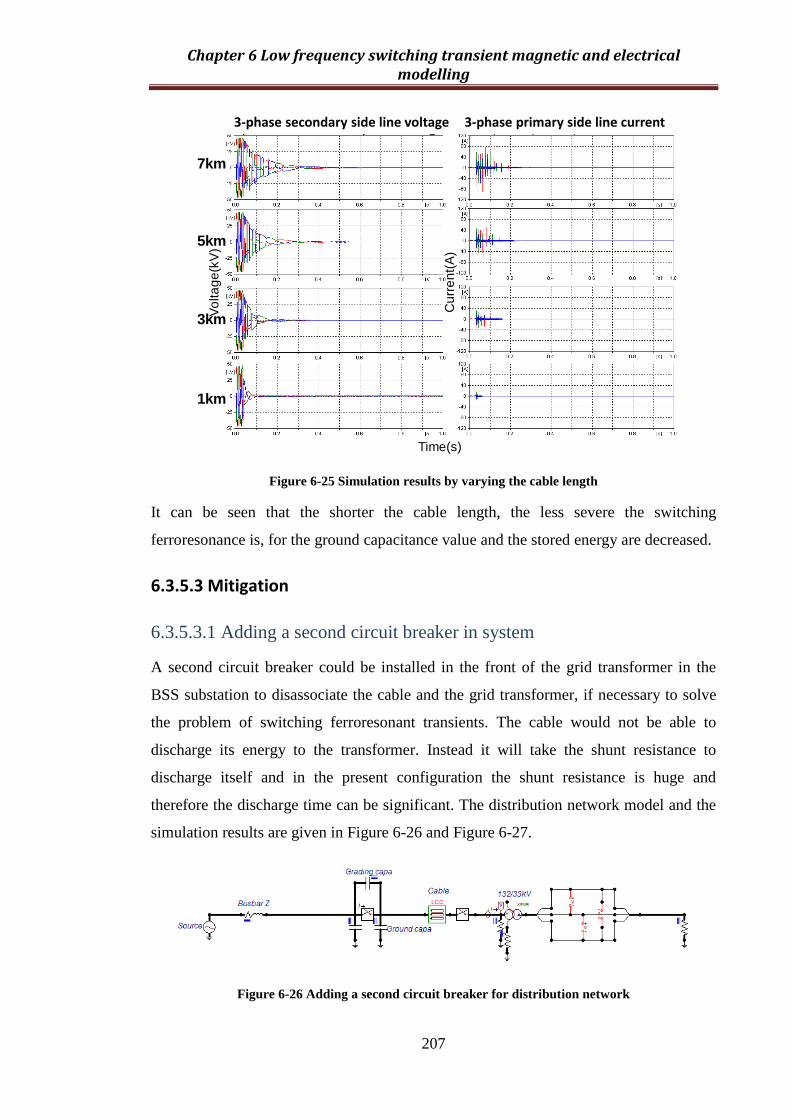
Chapter 6 Low frequency switching transient magnetic and electrical modelling
207
Figure 6-25 Simulation results by varying the cable length
It can be seen that the shorter the cable length, the less severe the switching
ferroresonance is, for the ground capacitance value and the stored energy are decreased.
6.3.5.3 Mitigation
6.3.5.3.1 Adding a second circuit breaker in system
A second circuit breaker could be installed in the front of the grid transformer in the
BSS substation to disassociate the cable and the grid transformer, if necessary to solve
the problem of switching ferroresonant transients. The cable would not be able to
discharge its energy to the transformer. Instead it will take the shunt resistance to
discharge itself and in the present configuration the shunt resistance is huge and
therefore the discharge time can be significant. The distribution network model and the
simulation results are given in Figure 6-26 and Figure 6-27.
Figure 6-26 Adding a second circuit breaker for distribution network
Vo
lta
ge
(kV
)
Cu
rre
nt(
A)
Time(s)
3-phase line secondary side voltage 3-phase primary side current
1km
3km
5km
7km
3-phase secondary side line voltage 3-phase primary side line current

Chapter 6 Low frequency switching transient magnetic and electrical modelling
208
Figure 6-26 shows the circuit diagram with the added circuit breaker at the front of the
grid transformer. If the transformer goes through the routine maintenance, the first step
of the operation should be to open the 33 kV circuit breaker; the second step should be
to open the 132kV CB in front of the grid transformer.
Figure 6-27 shows the simulation results including the cable voltages, the secondary
side voltages of the transformer, the second circuit breaker currents and the primary side
currents of the transformer. The transformer has not oscillated and there is no
overvoltage and overcurrent occurring in the system.
Figure 6-27 Simulation results: (a) three-phase cable voltages; (b) three-phase secondary side line
voltages; (c) three-phase circuit breaker currents; (d) three-phase primary side currents
6.3.5.3.2 Adding a parallel resistor bank at secondary side of system
The previous solution using the second circuit breaker is not economic, due to the cost
of the circuit breaker. Another solution is to add a parallel resistance load at the
secondary side of the transformer [16]. The resistance bank can be only switched in
whenever the grid transformer needs to be disconnected. Prior to switching operation,
the resistance bank is switched into the circuit to prepare for the operation, the circuit of
the modified model after shedding the load is shown in Figure 6-28.
Time(ms)
Cu
rre
nt(
A)
Time(s)
Vo
ltag
e(k
V)
Time(ms)
Cu
rre
nt(
A)
Time(s)
Vo
ltag
e(k
V)
(a) (b)
(c) (d)

Chapter 6 Low frequency switching transient magnetic and electrical modelling
209
Figure 6-28 Adding parallel resistor for distribution network
It can be seen from Figure 6-29 that the voltages and the currents damped quickly and
there are slight overvoltages lasting for less than a cycle here. The magnitude of the
current reaches 50 A, but it is still lower than the ferroresonance current and also lowers
than the full load current. The voltage damped within one cycle, the current is sin wave
which means that the transformer works at the linear and is not caused by
ferroresonance.
Figure 6-29 Simulation results: (a) three-phase line voltages at secondary side; (b) primary side
currents
The suitable resistance bank has a resistance value of 200 Ohm.
6.4 Case 2: Red bank substation circuit
6.4.1 Introduction
Base on the modelling experience for the Bloom Street Substation, the Red Bank
Substation model has been built in order to predict the ferroresonant transient
phenomenon in this circuit system.
The Red Bank circuit has the same configuration as the Bloom Street Substation case;
however there is a long cable connected between the transformer and the circuit breaker.
The cable used is the oil-fed cable.
Time(ms)
Cu
rre
nt(
A)
Time(s)
Vo
ltag
e(k
V)
(a) (b)

Chapter 6 Low frequency switching transient magnetic and electrical modelling
210
Figure 6-30 Whitegate Substation and Red Bank Substation layout
Figure 6-31 shows the comparison between the Bloom Street circuit and the Red Bank
circuit.
Figure 6-31 Comparison of single line diagram of the Bloom Street and Red Bank circuit
It can be seen that both of them are built with a 132 kV busbar, 132 kV SF6 circuit
breaker, a long distance 132 kV cable a 132/33 kV YNd connected transformer, an
earthing transformer and a voltage transformer.
The likelihood of inducing the same phenomenon as in Bloom Street Substation and
Preston East Substation is quite high, so simulation studies were conducted and the
comparison is made.
substationRed Bank
Underground cable
Whitegate(132 kV)
(33 kV)
Ground
Preston East
Bloom Street
Red Bank
System Configuration:
- same
Voltage level:
- same

Chapter 6 Low frequency switching transient magnetic and electrical modelling
211
6.4.2 Simulation and comparison
This circuit can be simplified by ignoring closed isolators and opened earth switches so
that it consists of the main components such as a 132 kV voltage source, CB, cable and
grid transformer. The connected auxiliary transformer, 33kV cable and 33kV VT are
further neglected since they bear negligible consequences. The model is shown in
Figure 6-32.
Figure 6-32 ATP simulation model of Red Bank circuit
Table 6-8 shows the source impedance at the busbar in the 132 kV substations. It can be
seen that both of the resistances are the same in those two circuits, and the inductances
are slightly different.
Table 6-8 132 kV three-phase fault level comparison between Bloom Street case and Red Bank case
Figure 6-33 shows the comparison between the two transformers operating in the two
different circuits, i.e. the transformer test reports for the open circuit test and short
circuit test. It can be seen that although the two transformers are manufactured by two
different manufacturers, the open circuit and short circuit test results are similar to each
other.

Chapter 6 Low frequency switching transient magnetic and electrical modelling
212
Figure 6-33 Comparison of two transformers’ data
Figure 6-34 shows the comparison between the XLPE cable used to connect with
Bloom Street Substation and the oil-fed cable used to connect with Red Bank Substation.
Figure 6-34 Comparison of the data of two cables
It can be seen that the capacitance value of the oil-feed cable is almost twice as high as
the XLEP one. The cable length in the Red Bank circuit is slightly longer than the
Bloom Street circuit. It can be expected that the magnitude of ferroresonant transients
would be higher in the Red Bank one and the resonance period would be longer than the
Bloom Street Substation.
Since both of the circuits use 132 kV circuit breakers from the same manufacturer, the
simulation is carried out by using the same opening time (phase A=0.0292, phase
B=0.0301, phase C=0.0301) and chopping current (30 Amp)as those used in the Bloom
Street case. The simulation results are shown in Figure 6-35. Figure 6-35 (a) is the
secondary side line voltages and (b) is the primary side currents.
Bloom Street
Red Bank
Type Length ConfigurationSubstation Capacitance
173 pF/m XLPE 9.55 km
335 pF/m Oil-Feed 11.5 km
3 single core cable
3-core cable in a pipe

Chapter 6 Low frequency switching transient magnetic and electrical modelling
213
Figure 6-35 Simulation results of Red Bank (a) secondary side line voltages (b) primary side
currents
It can be seen that the comparison suggests that between the two types of cable singe-
core XLPE cable and the three-core oil-fed cable, the oil-fed cable has more energy
(higher capacitance) and takes longer for the transient ferroresonance to damp than the
XLPE cable.
The currents approximately follow a 1:-0.5:-0.5 magnitude ratio and the waveforms are
quite similar. When the core is in the linear region, the currents of three phases are zero
sequence currents and the peak value is around 6 A and the frequency is around 400 Hz.
The current takes around 0.8 s to be damped.
Figure 6-36 shows that varying the cable length the ferroresonance of the secondary
side voltage waveforms and the primary side current waveforms. Compared with the
Bloom Street case, the transient ferroresonance takes longer to damp than the XLPE
cable for the same length cable. 1 km of oil-fed cable can create a three cycle
ferroresonance.
Time(s)
Cu
rre
nt(
A)
Time(s)
Vo
ltag
e(k
V)

Chapter 6 Low frequency switching transient magnetic and electrical modelling
214
Figure 6-36 Simulation results by varying the cable length
6.5 Summary
In this chapter, each main component of the distribution network has been modelled
using test report data and design data. In order to have a valid model which produces
matching results to the field recorded data, parameters have been trailed with slight
modifications such as the current chopping of circuit breaker, transformer λ-I curves
and resistive losses. Although ATP simulation eventually presented reasonable results
which matched with the recorded test data, ferroresonant transient phenomena are
complex multi-parameter controlled and we cannot be certain that the simulation
conditions which produced matching results are realistic situations when the tests were
performed.
However, general knowledge can be obtained on the switching ferroresonant transient
phenomena. During normal de-energisation events, interaction between the circuit
breaker, the cable and the transformer in this distribution network configuration results
in a ferroresonant transient phenomenon. In nature, the transient ferroresonance is due
to the fact that the energy stored in the cable capacitance discharges itself via the
transformer core inductance and causes core saturation. Since the energy source (cable
capacitance) is a limited one, the ferroresonance will not be sustained. Depending on the
5km
2km
1km
Vo
lta
ge
(kV
)
Cu
rre
nt(
A)
Time(s)
3km
3-phase line secondary side voltages 3-phase primary side currents

Chapter 6 Low frequency switching transient magnetic and electrical modelling
215
coordination of the three-phase switching time of the circuit breaker, fine differences
can exist between ferroresonant voltage and current waveforms.
From the previous field recorded results and simulation analysis, it is clear that the
unusual noise heard when de-energising the off-load transformer is due to core
saturation and ferroresonance. However, detailed analysis indicates that there is no
overvoltage on the transformer terminals and the highest saturation magnetising current
is about 130 A in peak, which is much higher than the normal magnetising current (Im =
0.98 A) but less than the full load current (IL = 396 A).
The potential damage of this ferroresonant transient phenomenon is therefore not caused
by overvoltage or overcurrent; instead it can be due to the fact that the flux was forced
to go through other paths as well as the core. Overfluxing and its side effects of
producing induced eddy currents and local heat concentration can be a long-term ageing
factor. However the total energy dumped into the transformer during the short lasting
time of transient (t = 0.62 s) is only 50 kJ, which is higher than the no-load loss but
much lower than the load-loss. From this comparison it seems reasonable to conclude
that the heating effect may not be significant due to the transient nature of
ferroresonance upon de-energisation.
In terms of the overfluxing and the flux leak, they are likely to occur near to the core
joints. During the investigative field tests acoustic sensors from Physical Acoustics Ltd
were used in an attempt to locate the source of the audible noise. However the acoustic
emission from the de-energisation event is relatively low and the acoustic emission did
not hit enough sensors to allow a 3D location. The DGA analysis on the oil samples was
normal, and there was no trace increase of any overheating gases in the oil samples
taken before and after the tests.
Transient interaction among transformers and other system components during
energisation and de-energisation are becoming increasingly important, due to the
increased generation connection and the reinforcing network activities.
Although computer simulation can be successfully employed to investigate the root
cause of the switching transient ferroresonance, it is recommended that the following is
necessary in order to develop a simulation model more accurately: (1) Measuring the
current and voltage at the primary side: high frequencies cannot pass through windings

Chapter 6 Low frequency switching transient magnetic and electrical modelling
216
without distortion, (2) Making synchronised time control: record exactly the circuit
opening time, the “cluck” noise appearing time, (3) Measuring current passing through
the circuit breaker since CB behavior to break small capacitive and inductive currents
are unknown and worth studying.

Chapter 7 Conclusion and further work
217
Chapter 7 Conclusion and further
work
7.1 Conclusion
7.1.1 General
This thesis described extensive simulation studies carried out on GIC and low frequency
switching transient phenomena where the effects of the transformer design and the
network parameters were identified. The main objective of this thesis is to investigate
the sensitivity of transformer structure design when it meets the GIC events and the
switching transient’s phenomena. The key technical challenge is associated with the
transformer core saturation.
The overall thesis work consists of the following parts:
1. To build a mathematical magnetic circuit model based on the principle of duality;
in particular to develop and validate a three-limb transformer core model having
zero-sequence flux return path, so it can be used to simulate the flux distribution
inside the transformer under the unbalanced situation;
2. To build a model in ATPDraw which is able to describe the system network
including transformers and other system components under GIC events;
3. To perform sensitivity studies on different network circuit parameters with
different transformer structures in order to investigate their influences on the
transformer saturation level, the saturation currents, the saturation time and the
sustained current waveforms;
4. To build a network model in ATPDraw based on the general distribution
network configuration, and validate the model with the field test results; and to
conduct the sensitivity study.
7.1.2 Summary of results and main findings
The influence of transformer core structure on the magnetising current under DC bias or
GIC events have been successfully identified. Starting with a statistical analysis of the

Chapter 7 Conclusion and further work
218
National Grid database of the transformer open circuit test results, it was found that core
material improvement has reduced the magnitude of the magnetising current over the
last few decades. There are two common types of transformer core structures: three-
limb and five-limb cores influence the balance of three-phase magnetising currents. In
addition, the winding connection; Y or D would influence the magnetising currents.
The simulation cases show that for the five-limb transformer, three-phase magnetising
currents are much better balanced than those of the three-limb transformer; and the
magnitude of the magnetic flux density of the main yoke is higher than in the main limb
and side yoke in the five-limb transformer core. The magnitude of the fundamental
frequency magnetic flux density in the side yoke is changing faster than that in the main
yoke with the change of the supplied voltage; the ratio of the cross-section between the
main yoke and the side yoke would influence the magnitude of fundamental frequency
and third harmonic flux distribution in the five-limb transformer core. The higher the
ratio between the main yoke and the side yoke, the more difficult it would take the
transformer to become saturated. However, the main yoke length is almost twice that of
the side yoke; so if the area of the main yoke is increased, it would cost more to buy
core materials and become harder for the transformer to transport.
Although the transformer manufacturers provide the RMS values of the magnetising
currents, without the detailed waveform, the information is not sufficient to understand
the flux distribution in the core. The recommendation is then made in this research that
the manufacturers should provide the detail of the magnetising current waveforms for
90%, 100% and 110% voltage levels during the open circuit tests.
By using the EMTP-ATPDraw transient calculation software, a network system was
built to analyse GIC events and it can be seen that the step time of the primary side
current is influenced by the winding connection, the core structure and the transformer
zero sequence impedance. It can be summarised that the ‘one-step function’ waveform
only appears for a single phase transformer with the YNy winding connection; the ‘two-
step function’ waveform appears for a single phase transformer and a three-phase three-
limb transformer with the YNd winding connection and a five-limb transformer with the
YNy winding connection; the ‘three-step function’ waveform appears for a five-limb
transformer with a three winding YNad or a two winding YNd connection.
Transformer winding impedance controls the behaviour of the primary side current.
Winding impedance combined with DC supply level decides the time constant and the
Chapter 7 Conclusion and further work
219
stable value of the step response. The system impedance gives the same effect as the
winding impedance. The core saturation characteristics mainly control the saturation
stage, including the speed of the rise and the time for the saturation.
The zero sequence impedance also plays an important role in this phenomenon.
Different structures of transformers have different characteristics from the zero
sequence impedance. The three-phase three-limb transformer is more complex than that
of the three single-phase transformers bank, i.e. the DC flux cannot find a return path
inside of the core and has to leak out of the core and circulate through the oil and tank.
The zero sequence impedance in the three-limb transformer affects the step response
time constant and the stable value and it also impacts the saturation time by influencing
the DC voltage drop on the transformer core.
For a three-phase five-limb transformer, the ‘three-step function’ waveform appears
with a YNd winding connection. For the first step, the DC flux is accumulated inside
the core through the side yoke, which then has a different reluctance from the positive
sequence core reluctance. For the second step, all DC flux continues the accumulation
and flows through the side yoke until the side yoke is saturated. The saturation of the
side yoke causes the second rise of the primary current. After the side yoke is saturated,
the five-limb transformer tends to behave like a three-limb transformer. For the last step,
DC flux increases further in the transformer core; the entire core goes into saturation.
As a result, the total non-linear core inductance starts to decrease and the primary side
current grows swiftly.
As for another core saturation problem named ferroresonance, it was found that
ferroresonant transients are complex multi-parameter controlled phenomena which
include the circuit breaker chopping current, its opening time and the grading
capacitance, the cable length and the transformer core characteristics. During normal
de-energisation events, interaction between the circuit breaker, the cable and the
transformer in the typical distribution network configuration results in a ferroresonant
transient phenomenon. In nature, the transient ferroresonance is due to the fact that the
energy stored in the cable capacitance discharges itself via the transformer core
inductance and causes core saturation. Since the energy source (cable capacitance) is a
limited one, the ferroresonance will not be sustained. Depending on the coordination of
the three-phase switching times of the circuit breaker, fine differences can exist on
ferroresonant voltage and current waveforms.

Chapter 7 Conclusion and further work
220
Based on the field recorded results and simulation analysis, it is clear that the unusual
noise heard when de-energising the off-load transformer is due to core saturation and
ferroresonance. However detailed analysis indicates that there is no overvoltage on the
transformer terminals and the highest saturation magnetising current is about 130 A in
peak, which is much higher than the normal magnetising current (Im = 0.98 A) but less
than the full load current (IL = 396 A). The potential damage of this ferroresonant
transient phenomenon is therefore not caused by overvoltage or overcurrent; instead it
can be due to the fact that the flux was forced to go through other paths as well as the
core.
Overfluxing and its side effects of producing induced eddy currents and local heat
concentration can be a long-term ageing factor. However the total energy dumped into
the transformer during the short lasting time of transient (t = 0.62 s) is only 50 kJ, which
is higher than no-load loss but much lower than the load-loss. From this comparison it
seems reasonable to conclude that the heating effect may not be significant due to the
transient nature of ferroresonance upon de-energisation.
More importantly, in terms of overfluxing and flux leak, they are likely to occur near to
the core joints. During the investigative field tests acoustic sensors from Physical
Acoustics Ltd were used in an attempt to locate the source of the audible noise.
However the acoustic emission from the de-energisation event is relatively low and the
acoustic emission did not hit enough sensors to allow a 3D location. The DGA analysis
of the oil samples was normal, and there was no trace increase of any overheating gases
in the oil samples taken before and after the tests.
7.2 Further work
The work presented in this thesis indicates that the overall approach of modelling
transformer core has helped the interpretation of core saturation problems; however
further work could be carried out on the following points:
As mentioned in Chapter 3, the transformer core model used in this thesis neglected the
losses of the transformer core material and also the building/structuring effect of core,
i.e. at the core joint areas. This model is a pure magnetic circuit model for the moment,
so the electrical part should be added into the model in the future. Once the model is
Chapter 7 Conclusion and further work
221
combined with both of the electrical and magnetic circuits, it can be used to calculate
both the balanced and the unbalanced studies.
When the manufacturer does the open circuit test for a transformer, only the RMS
values of the supplied voltages and the RMS values of the magnetising currents are
recorded. If the transformer core is working in the knee area or the saturation region,
only recording the RMS values is not accurate enough for the data to be used or
extrapolated to represent the transformer core characteristic which is a necessity for the
simulation model especially when studying the behaviours of transformer under
saturation. Unless the manufacturers can provide those data, the transformer model and
the simulation results could not be further improved.
The benefit of the mathematical model introduced in Chapter 3 can show the flux
distribution in the transformer and the ATPDraw could not do this at the moment. If the
mathematical model can be applied into ATPDraw as an external coded model, it would
massively improve the ATPDraw software.
The present models built up in the ATPDraw do not consider the non-linear core losses
in the transformer; instead it uses a linear resistor to represent the core losses. And a
parallel resistor is connected with the transformer core. In the future work the
transformer model should be further improved using the dynamic value of core losses.

Reference
222
Reference [1] CIGRE, "Guidelines for Representation of Network Elements when Calculating
Transients," WG 33.02 vol. 039, 1990.
[2] Greenwood.Allan, "Electrical Transients in Power Systems," 1991.
[3] A. Pors and N. Browne, "Modelling the Energisation of a Generator Step-up
Transformer from the High Voltage Network," presented at the Australasian
Universities Power Engineering Conference, 2008.
[4] M. Heathcote, "J & P Transformer Book," 1998.
[5] L. F. Blume, G. Camilli, S. B. Farnham, and H. A. Peterson, "Transformer
Magnetizing Inrush Currents and Influence on System Operation," Transactions
of the American Institute of Electrical Engineers, vol. 63, pp. 366-375, 1944.
[6] D. Povh and W. Schultz, "Analysis of Overvoltages Caused by Transformer
Magnetizing Inrush Current," IEEE Transactions on Power Apparatus and
Systems, vol. 97, pp. 1355-1365, 1978.
[7] M. Rioual and J. C. Reveret, "Energization of Step-up Transformers for Wind-
farms: Modeling and its Validation by Tests Performed on a 10 MW Site,"
presented at the IEEE Power & Energy Society General Meeting, Alberta,
Canada, 2009.
[8] L. Prikler, G. Bánfai, G. Bán, and P. Becker, "Reducing the Magnetizing Inrush
Current by Means of Controlled Energization and De-energization of Large
Power Transformers," Electric Power Systems Research, vol. 76, pp. 642-649,
2006.
[9] M. Nagpal, T. G. Martinich, A. Moshref, K. Morison, and P. Kundur,
"Assessing and Limiting Impact of Transformer Inrush Current on Power
Quality," IEEE Transactions on Power Delivery, vol. 21, pp. 890-896, 2006.
[10] Areva, "Power Transformers," Fundamentals, vol. 1, 2008.
[11] D. A. N. Jacobson, "Examples of Ferroresonance in a High Voltage Power
System," presented at the IEEE Power Engineering Society General Meeting,
2003.
[12] R. Zhang, T. Byrne, D. Jones, and Z. D. Wang, "A Technical Experience during
Network Asset Replacement: Investigating Cable and Transformer Switching
Interactions," presented at the CIRED, Lyon, France, 2010.
[13] E. J. Dolan, D. A. Gillies, and E. W. Kimbark, "Ferroresonance in a Transformer
Switched with an EHV Line," IEEE Transactions on Power Apparatus and
Systems, vol. 91, pp. 1273-1280, 1972.
[14] C. Charalambous, Z. D. Wang, M. Osborne, and P. Jarman, "Sensitivity Studies
on Power Transformer Ferroresonance of a 400 kV Double Circuit," IET on
Generation, Transmission & Distribution, vol. 2, pp. 159-166, 2008.
[15] Z. Emin, B. A. T. Al Zahawi, and Y. K. Tong, "Voltage Transformer
Ferroresonance in 275 kV Substation," presented at the Eleventh International
Symposium on High Voltage Engineering, London, UK, 1999.
[16] D. A. N. Jacobson, D. R. Swatek, and R. W. Mazur, "Mitigating Potential
Transformer Ferroresonance in a 230 kV Converter Station," presented at the
IEEE Transmission and Distribution Conference, Los Angeles, California, 1996.
[17] R. C. Dugan, "Examples of Ferroresonance in Distribution," presented at the
IEEE Power Engineering Society General Meeting, Toronto, Canada, 2003.
[18] C. B. K.Pattanapakdee, "Failure of Riser Pole Arrester due to Station Service
Transformer Ferroresonance," presented at the IPST'07, Lyon, France, 2007.

Reference
223
[19] R. Zhang, S. P. Ang, H. Li, and Z. D. Wang, "Complexity of Ferroresonance
Phenomena: Sensitivity Studies from a Single-phase System to Three-phase
Reality," presented at the International Conference on High Voltage Engineering
and Application, New Orleans, LA, USA, 2010.
[20] P. R. Barnes, D. T. Rizy, B. W. McConnel, F. M. Tesche, and E. R. Taylor,
"Electric Utility Industry Experience with Geomagnetic Disturbances," ed:
Oakridge National Laboratory, 1991.
[21] D. H. Boteler, R. J. Pirjola, and H. Nevanlinna, "The Effects of Geomagnetic
Disturbances on Electrical Systems at the Earth's Surface," Advances in Space
Research, vol. 22, pp. 17-27, 1998.
[22] T. S and Molinski, "Why Utilities Respect Geomagnetically Induced Currents,"
Journal of Atmospheric and Solar-Terrestrial Physics, vol. 64, pp. 1765-1778,
2002.
[23] J. G. Kappenman, "Geomagnetic Storms and their Impact on Power Systems,"
IEEE Power Engineering Review, vol. 16, p. 5, 1996.
[24] Z. D. Wang, "Msc Note on Power Transformer in University of Manchester,"
2011.
[25] ABB, "Transformer Handbook," Transformer Design, 2004.
[26] J. J. Winders, "Power Transformer Principles and Applications," 2002.
[27] D. Jiles, "Introduction to Magnetism and Magnetic Materials," 1991.
[28] M. A. Laughton and D. F. Warne, "Electrical Engineer's Reference Book (16th
Edition)," 2003.
[29] R. C. O'Handley, "Modern Magnetic Materials: Principles and Applications,"
2000.
[30] W. Storr, "Basic Electronics Tutorials Site," 2012.
[31] A. J. Moses, "Electrical Steels: Past, Present and Future Developments," IEE
Proceedings on A Physical Science, Measurement and Instrumentation,
Management and Education, vol. 137, pp. 233-245, 1990.
[32] C. A. Charalambous, Z. D. Wang, P. Jarman, and M. Osborne, "2-D Finite-
Element Electromagnetic Analysis of an Autotransformer Experiencing
Ferroresonance," IEEE Transactions on Power Delivery, vol. 24, pp. 1275-1283,
2009.
[33] "IEEE Standard for Ferroresonant Voltage Regulators," IEEE Std 449-1990, p.
0_1, 1990.
[34] J. Bethenod, "Sur Le Transformateur et Résonance," L' Eclairae Electrique, pp.
289-296, 1907.
[35] P. Boucherot, "Existence de Deux Régimes en Ferro-résonance," R.G.E., pp.
827-828, 1920.
[36] J. W. Butler and C. Concordia, "Analysis of Series Capacitor Application
Problems," Transactions of the American Institute of Electrical Engineers, vol.
56, pp. 975-988, 1937.
[37] R. Rüdenberg, "Transient Performance of Electric Power Systems: Phenomena
in Lumped Networks," 1969.
[38] C. Hayashi, "Nonlinear Oscillations in Physical Systems," 1985.
[39] Y. K. Tong, "NGC Experience on Ferroresonance in Power Transformers and
Voltage Transformers on HV Transmission Systems," presented at the IEE
Colloquium on Warning! Ferroresonance Can Damage Your Plant, Glasgow,
UK, 1997.

Reference
224
[40] S. P. ANG, "Ferroresonance Simulation Studies of Transmission Systems," PhD,
School of Electrical and Electronic Engineering, The University of Manchester,
2010.
[41] M. R. Iravani, A. K. S. Chaudhary, W. J. Giesbrecht, I. E. Hassan, A. J. F. Keri,
K. C. Lee, J. A. Martinez, A. S. Morched, B. A. Mork, M. Parniani, A. Sharshar,
D. Shirmohammadi, R. A. Walling, and D. A. Woodford, "Modeling and
Analysis Guidelines for Slow Transients. III. The study of Ferroresonance,"
IEEE Transactions on Power Delivery, vol. 15, pp. 255-265, 2000.
[42] W. H. Barlow, "On the Spontaneous Electrical Currents Observed in the Wires
of the Electric Telegraph," Philosophical Transactions of the Royal Society of
London, vol. 139, pp. 61-72, 1849.
[43] J. B. Wareing and F. Perrot, "Ferroresonance Overvoltages in Distribution
Networks," presented at the IEE Colloquium on Warning! Ferroresonance Can
Damage Your Plant, Glasgow, UK, 1997.
[44] Available: http://info.ee.surrey.ac.uk/Workshop/advice/coils/mu/
[45] C. A. Charalambous, R. Zhang, and Z. D. Wang, "Simulation Thermal
Conditionals around Core Bolts when Transformer is Experiencing
Ferroresonance," presented at the Intertnational Power System Transient
Conference, Delft, Holland, 2011.
[46] A. Wilson and J. A. Lapworth, "Defining the Life of Major Assets," presented at
the International Conference on Condition Monitoring and Diagnosis, Beijing,
China, 2008.
[47] R. H. Brierley, A. S. Morched, and T. E. Grainger, "Compact Right-of-ways
with Multi-voltage Towers," IEEE Transactions on Power Delivery, vol. 6, pp.
1682-1689, 1991.
[48] K. Pattanapakdee and C. Banmongkol, "Failure of Riser Pole Arrester due to
Station Service Transformer Ferroresonance," presented at the International
Conference on Power Systems Transients, Lyon, France, 2007.
[49] "IEEE Guide for the Interpretation of Gases Generated in Oil-Immersed
Transformers," IEEE Std C57.104-2008 (Revision of IEEE Std C57.104-1991),
pp. C1-27, 2009.
[50] G. B. Prescott, "History, Theory and Practice of the Electric Telegraph," 1866.
[51] Allison, N.J., and W.E.Huddleston, "Extraneous Currents Noted on Large
Transmission Pipe Line System," presented at the National Assoc. of Corrosion
Engineers, Houston, TX, 1952.
[52] T. G. Proctor, "Experience with Telluric Current Interference in the Cathodic
Protection of a Buried Pipeline in New Zealand " presented at the National
Assoc. of Corrosion Engineers, Houston, TX, 1974.
[53] J. G. Kappernman and V. D. Albertson, "Bracing for the Geomagnetic Storms,"
IEEE Spectrum, vol. 27, pp. 27-33, 1990.
[54] Czech, P.S.Chao, H. Huynh, and A. Dutil, "The Hydro-Quebec System Blackout
of 13 March 1989: System Response to Geomagnetic Disturbance," presented at
the Geomagnetically Induced Currents Conference, California, USA, 1992.
[55] John.Kappenman, "Geomagnetic Disturbances and Impacts upon Power System
Operation," 2007.
[56] J. J. Grainger and W. S. Jr., "Power System Analysis," 1994.
[57] "Geomagnetic Disturbance Effects on Power Systems," IEEE Transactions on
Power Delivery, vol. 8, pp. 1206-1216, 1993.
[58] P. O. Persson, "Disturbances in Directly Earthed Transmission Power Systems
Caused by Geomagnetic Storms," presented at the 3rd Symposium and

Reference
225
Technical Exhibition on Electromagnetic Compatibility, Rotterdam, Holland,
1979.
[59] D. H. Boteler, "Geomagnetic Hazards to Conducting Networks," Natural
Hazards, vol. 28, pp. 537-561, 2003.
[60] V. D. Albertson and J. C. Slothower, "The Effects of Solar Magnetic Activity on
Electric Power Systems," J. Minn. Acad. Sci., vol. 34, pp. 94-100, 1967.
[61] V. D. Albertson, J. M. Thorson, and S. A. Miske, "The Effects of Geomagnetic
Storms on Electrical Power Systems," IEEE Transactions on Power Apparatus
and Systems, vol. PAS-93, pp. 1031-1044, 1974.
[62] A. J. Pesonen, "Effects of Solar-Induced Currents on Power Systems - A Brief
Survey," presented at the CIGRE Study Committee 36, Madrid, Spain, 1979.
[63] "March 13, 1989 Geomagnetic Disturbance," 1990.
[64] J. A. Marusek, "Solar Storm Threat Analysis," presented at the Nuclear Physicist
and Engineer, Bloomfield, Indiana, 2007.
[65] D. Beamish, T. D. G. Clark, E. Clarke, and A. W. P. Thomson,
"Geomagnetically Induced Currents in the UK: Geomagnetic Variations and
Surface Electric Fields," Journal of Atmospheric and Solar-Terrestrial Physics,
vol. 64, pp. 1779-1792, 2002.
[66] A. W. P. Thomson, A. J. McKay, E. Clarke, and S. J. Reay, "Surface Electric
Fields and Geomagnetically Induced Currents in the Scottish Power Grid during
the 30 October 2003 Geomagnetic Storm," Space Weather, vol. 3, p. S11002,
2005.
[67] I. A. Erinmez, J. G. Kappenman, and W. A. Radasky, "Management of the
Geomagnetically Induced Current Risks on the National Grid Company's
Electric Power Transmission System," Journal of Atmospheric and Solar-
Terrestrial Physics, vol. 64, pp. 743-756.
[68] R. A. Walling and A. N. Khan, "Characteristics of Transformer Exciting-current
during Geomagnetic Disturbances," IEEE Transactions on Power Delivery, vol.
6, pp. 1707-1714, 1991.
[69] L. Bolduc, A. Gaudreau, and A. Dutil, "Saturation Time of Transformers under
DC Excitation," Electric Power Systems Research, vol. 56, pp. 95-102, 2000.
[70] P. R. Price, "Geomagnetically Induced Current Effects on Transformers," IEEE
Transactions on Power Delivery, vol. 17, pp. 1002-1008, 2002.
[71] N. Takasu, T. Oshi, F. Miyawaki, S. Saito, and Y. Fujiwara, "An Experimental
Analysis of DC Excitation of Transformers by Geomagnetically Induced
Currents," IEEE Transactions on Power Delivery, vol. 9, pp. 1173-1182, 1994.
[72] S. Lu and Y. Liu, "FEM Analysis of DC Saturation to Assess Transformer
Susceptibility to Geomagnetically Induced Currents," IEEE Transactions on
Power Delivery, vol. 8, pp. 1367-1376, 1993.
[73] L. Shu, L. Yiu, D. La, and J. Ree, "Harmonics Generated From A DC Biased
Transformer," presented at the V International Conference on Harmonics in
Power Systems Atlanta GA, 1992.
[74] D. Xuzhu, L. Yilu, and J. G. Kappenman, "Comparative Analysis of Exciting
Current Harmonics and Reactive Power Consumption from GIC Saturated
Transformers," presented at the IEEE Power Engineering Society Winter
Meeting, Columbus, Ohio, USA, 2001.
[75] W. G. Ireson, C. F. Coombs, and Moss, "Handbook of Reliability Engineering
and Management," 1996.
[76] J. G. Kappenman, S. R. Norr, G. A. Sweezy, D. L. Carlson, V. D. Albertson, J.
E. Harder, and B. L. Damsky, "GIC Mitigation: a Neutral Blocking/bypass

Reference
226
Device to Prevent the Flow of GIC in Power Systems," IEEE Transactions on
Power Delivery, vol. 6, pp. 1271-1281, 1991.
[77] W. C. Viana, R. J. Micaleff, S. Young, F. P. Dawson, and E. P. Dick,
"Transformer Design Considerations for Mitigating Geomagnetic Induced
Saturation," IEEE Transactions on Magnetics, vol. 35, pp. 3532-3534, 1999.
[78] A. A. Fardoun, E. F. Fuchs, and M. A. S. Masoum, "Experimental Analysis of a
DC Bucking Motor Blocking Geomagnetically Induced Currents," IEEE
Transactions on Power Delivery, vol. 9, pp. 88-99, 1994.
[79] M. Chengxiong, W. Sheng, L. Jiming, M. Guihua, and W. Dan, "Measures of
Restraining DC Current Through Transformer Neutral Point: A Comprehensive
Survey," presented at the 42nd International Universities Power Engineering
Conference, Brighton, UK, 2007.
[80] N. Ben, Z. Rong, Z. Bo, and H. Jinliang, "Research and Design of the Neutral
Series Resistor to Restrain the HVDC Ground Current Flowing into
Transformer," presented at the International Conference on Power System
Technology, Chongqing, China, 2006.
[81] M. A. Eitzmann, R. A. Walling, M. Sublich, A. H. Khan, H. Huynh, M. Granger,
and A. Dutil, "Alternatives for Blocking Direct Current in AC System Neutrals
at the Radisson/LG2 Complex," IEEE Transactions on Power Delivery, vol. 7,
pp. 1328-1337, 1992.
[82] L. Bolduc, M. Granger, G. Pare, J. Saintonge, and L. Brophy, "Development of a
DC Current-blocking Device for Transformer Neutrals," IEEE Transactions on
Power Delivery, vol. 20, pp. 163-168, 2005.
[83] IEC, "Instrument transformers - Part 1: Current transformers," 60044-1:1996,
1996.
[84] J. Kappenman, "Geomagnetic Storms and Their Impact on U.S. Power Grid,"
2010.
[85] G. Stokes, "Handbook of Electrical Installation Practice," 2003.
[86] G. F. Moore, "Electric Cables Handbook (3rd Edition)," 1997.
[87] "Comparison Between Vacuum and SF6 Circuit Breaker,"
http://www.csanyigroup.com/comparison-between-vacuum-and-sf6-circuit-
breaker, 2009.

Appendix
227
Appendix
1 Matlab Code
clc clear all
%Inputing transformer basic parameters % 400/275/13kV, 1000MVA Transformer, working on Bm = 1.694T % Base on E=4.44*f*Bm*A1*N % Ibase=1000MVA/(400kV*1.732) % 400kv=4.44*50*1.694*0.70138*N*¡Ì3 % Calculation of Turn NO. for total winding together=965(real=960) % 965/(400/¡Ì3/13)=54 % Calculation of Turn NO. for tertariy winding = 54 % Core Material 27M4 % Original data of transfomrer % Main limb cross-section area/m2 0.6438 % Main yoke cross-section area /m2 0.3884 % Side limb cross-section area /m2 0.3884 % leg length (l1) = 2.79 m % Main yoke length (l2) = 2.57 m % Side yoke length (l3) = 1.6475 m
% Ratio Area of side limb(A3) Area of main yoke(A2) % 0.5:0.5 0.3219 0.3219 % 0.45:0.55 0.28971 0.35409 % 0.4:0.6 0.25752 0.38628 % 0.35:0.65 0.22533 0.41847 % 0.3:0.7 0.19314 0.45066
l1 = 2.79; l2 = 2.57; l3 = 1.6475; A1 = 0.6438; A2 = 0.3219; A3 = 0.3219; %initializing the intial condition a=1; x=1; z=1; m=1; k=1; Bm = 1.3; f = Bm*A1; flux(z,1)=f; e = 1e-10; t = 0; w=2*pi*50; np=965; nt=54;
%Inserting the B-H curve parameter 27M4 material A = 20; B = 6.46919e-5;

Appendix
228
while t<=0.04 %Checking the intial condition
fa(a,1) = f*cos (w*t)+0.2; fb(a,1) = f*cos (w*t - 2.0944)+0.2; fc(a,1) = f*cos (w*t + 2.0944)+0.2;
f1(x,1) = f-20; B1(x,1) = f1(x,1)/A3; B2(x,1) = ( f1(x,1) - fa(a,1))/A2; B3(x,1) = ( -f1(x,1) + fa(a,1) + fb(a,1))/A2; B4(x,1) = ( -f1(x,1) + fa(a,1) + fb(a,1) + fc(a,1))/A3;
H1(x,1) = A*(B1(x,1)) + B*((B1(x,1))^27); H2(x,1) = A*(B2(x,1)) + B*((B2(x,1))^27); H3(x,1) = A*(B3(x,1)) + B*((B3(x,1))^27); H4(x,1) = A*(B4(x,1)) + B*((B4(x,1))^27);
Ba(a,1) = fa(a,1)/A1; Bb(a,1) = fb(a,1)/A1; Bc(a,1) = fc(a,1)/A1;
Ha(a,1) = A*(Ba(a,1)) + B*((Ba(a,1))^27); Hb(a,1) = A*(Bb(a,1)) + B*((Bb(a,1))^27); Hc(a,1) = A*(Bc(a,1)) + B*((Bc(a,1))^27);
y(x,1)= H1(x,1)*(l1+2*l3) + H2(x,1)*2*l2 - H3(x,1)*2*l2 -
H4(x,1)*(2*l3+l1);
% Calculate few points for Newton-Raphson method initial value for x=1:4 f1(x+1,1)= f1(x,1) - 20; B1(x+1,1) = f1(x+1,1)/A3; B2(x+1,1) = ( f1(x+1,1) - fa(a,1))/A2; B3(x+1,1) = ( -f1(x+1,1) + fa(a,1) + fb(a,1))/A2; B4(x+1,1) = ( -f1(x+1,1) + fa(a,1) + fb(a,1) + fc(a,1))/A3;
H1(x+1,1)= A*(B1(x+1,1)) + B*((B1(x+1,1))^27); H2(x+1,1)= A*(B2(x+1,1)) + B*((B2(x+1,1))^27); H3(x+1,1)= A*(B3(x+1,1)) + B*((B3(x+1,1))^27); H4(x+1,1)= A*(B4(x+1,1)) + B*((B4(x+1,1))^27);
y(x+1,1)= H1(x+1,1)*(l1+2*l3) + H2(x+1,1)*2*l2 -
H3(x+1,1)*2*l2 - H4(x+1,1)*(2*l3+l1); x=x+1; end
while abs(y(x,1)) >= e % Newton-Raphson method to do the iteration f1(x+1,1)= f1(x,1) - (y(x,1)*(f1(x,1)-f1(x-1,1))/(y(x,1)-y(x-
1,1)));
B1(x+1,1) = f1(x+1,1)/A3;

Appendix
229
B2(x+1,1) = ( f1(x+1,1) - fa(a,1))/A2; B3(x+1,1) = ( -f1(x+1,1) + fa(a,1) + fb(a,1))/A2; B4(x+1,1) = ( -f1(x+1,1) + fa(a,1) + fb(a,1) + fc(a,1))/A3;
H1(x+1,1)= A*(B1(x+1,1)) + B*((B1(x+1,1))^27); H2(x+1,1)= A*(B2(x+1,1)) + B*((B2(x+1,1))^27); H3(x+1,1)= A*(B3(x+1,1)) + B*((B3(x+1,1))^27); H4(x+1,1)= A*(B4(x+1,1)) + B*((B4(x+1,1))^27);
y(x+1,1)= H1(x+1,1)*(l1+2*l3) + H2(x+1,1)*2*l2 -
H3(x+1,1)*2*l2 - H4(x+1,1)*(2*l3+l1); x=x+1
end
%Pick up the suitable value from the circle and pun into new array Bfit1(m,1)=B1(x-1,1); Hfit1(m,1)=H1(x-1,1); Bfit2(m,1)=B2(x-1,1); Hfit2(m,1)=H2(x-1,1); Bfit3(m,1)=B3(x-1,1); Hfit3(m,1)=H3(x-1,1); Bfit4(m,1)=B4(x-1,1); Hfit4(m,1)=H4(x-1,1);
Hfita(m,1)= Ha(a,1)*l1 + Hfit1(m,1)*(2*l3+l1); Hfitc(m,1)= Hc(a,1)*l1 + Hfit4(m,1)*(2*l3+l1); Hfitb(m,1)= Hb(a,1)*l1 + 2*Hfit2(m,1)*l2 + Hfit1(m,1)*(2*l3+l1);
Ia(m,1)=Hfita(m,1)/np; Ib(m,1)=Hfitb(m,1)/np; Ic(m,1)=Hfitc(m,1)/np;
Hmin(m,1)= (Hfit2(m,1)+ Hfit3(m,1))* l2; Haa(m,1)= Ha(a,1)*l1; tt(a,1)=t; a=a+1; t=t+0.0001; m=m+1;
end % plot the flux density for each part of transformer Current= [Ia Ib Ic]; figure(1) plot(tt, Hfit1,'--r',tt, Hfit2,'y',tt, Hfit3,'b',tt,Hfit4,'--
g','LineWidth',3.5) grid % Labels are erased, so generate them manually title('Mangetic field intensity(No-Delta)','FontSize',13) xlabel('Time(s)','FontSize',13) ylabel('H(A/m)','FontSize',13) % Add a legend in the upper left legend('H1','H2','H3','H4','Location','northeast')
figure(2) plot(Hfita,Ba,'r',Hfitb,Bb,'y',Hfitc,Bc,'b','LineWidth',3.5) grid % Labels are erased, so generate them manually

Appendix
230
title('B-H Characteristic in each phase(No-Delta)','FontSize',13) xlabel('H(A/m)','FontSize',13) ylabel('B(T)','FontSize',13) % Add a legend in the upper left legend('PhaseA','PhaseB','PhaseC','Location','northwest')
figure(3) plot(tt,Hfita,'r',tt,Hfitb,'y',tt,Hfitc,'b',tt,200*Ba,'--
r',tt,200*Bb,'--y',tt,200*Bc,'--b','LineWidth',3.5); grid % Labels are erased, so generate them manually title('Mangetic field intensity and Mangetic flux density(No-
Delta)','FontSize',13) xlabel('Time(s)','FontSize',13) ylabel('Ni(A) or B(200*T)','FontSize',13) % Add a legend in the upper left legend('Nia','Nib','Nic','Ba','Bb','Bc','Location','northeast')
% calculate FFT FFTA=fft(Ia); M1=abs(FFTA)*2/400; % obtain the magnitude value of each frequency Phase1=angle(FFTA)*180/pi; % obtain the angle value of each frequency % Pick the fundanmental frequency and harmorinic for i=1:21 MP1(i) = FFTA(1+2*(i-1)); Mhar1(i) = M1(1+2*(i-1)); % 1/(total time) is the fundamental
harmonic frequency, collecting the 50 Hz and Odd harmonics Phar1(i) = Phase1(1+2*(i-1)); end % plot magnitude value of fundanmental frequency and harmorinic
f1=0:50:1000; figure(4) stem(f1,Mhar1,'r','LineWidth',3.5); grid; % Labels are erased, so generate them manually title('Mangetizing Current Frequency Contain in Phase A(No-
Delta)','FontSize',13) xlabel('Frequency(Hz)','FontSize',13) ylabel('Magnitude of Current(A)','FontSize',13) %figure(5) %stem(f1,Phar1); %grid;
FFTB=fft(Ib); M2=abs(FFTB)*2/400; % obtain the magnitude value of each frequency Phase2=angle(FFTB)*180/pi; % obtain the angle value of each frequency % Pick the fundanmental frequency and harmorinic for i=1:21 MP2(i) = FFTB(1+2*(i-1)); Mhar2(i) = M2(1+2*(i-1)); Phar2(i) = Phase2(1+2*(i-1)); end
figure(5) stem(f1,Mhar2,'y','LineWidth',3.5); grid;
Appendix
231
% Labels are erased, so generate them manually title('Mangetizing Current Frequency Contain in Phase B(No-
Delta)','FontSize',13) xlabel('Frequency(Hz)','FontSize',13) ylabel('Magnitude','FontSize',13)
FFTC=fft(Ic); M3=abs(FFTC)*2/400; % obtain the magnitude value of each frequency Phase3=angle(FFTC)*180/pi; % obtain the angle value of each frequency % Pick the fundanmental frequency and harmorinic for i=1:21 MP3(i) = FFTC(1+2*(i-1)); Mhar3(i) = M3(1+2*(i-1)); Phar3(i) = Phase3(1+2*(i-1)); end
PhaseABC= [Phar1' Phar2' Phar3'];
figure(6) stem(f1,Mhar3,'b','LineWidth',3.5); grid; title('Mangetizing Current Frequency Contain in Phase C(No-
Delta)','FontSize',13) xlabel('Frequency(Hz)','FontSize',13) ylabel('Magnitude','FontSize',13)
%Calculate the Zero, Positive and Nagative sequence
for i=1:21 III=[MP1(1,i);MP2(1,i);MP3(1,i)]; AA=[1,1,1;1,complex(-0.5,0.866),complex(-0.5,-0.866);1,complex(-
0.5,-0.866),complex(-0.5,0.866)]; Izpn = AA*III/3; Izero (1,i)= Izpn(1,1); Iposi (1,i)= Izpn(2,1); Inaga (1,i)= Izpn(3,1); MIzero(1,i)=abs(Izero(1,i))*2/400; MIposi(1,i)=abs(Iposi(1,i))*2/400; MInaga(1,i)=abs(Inaga(1,i))*2/400; end
hba= [Hfita Ba]; hbb= [Hfitb Bb]; hbc= [Hfitc Bc]; hb= [Hfita Ba Hfitb Bb Hfitc Bc];
HarmonicA= Mhar1'; HarmonicB= Mhar2'; HarmonicC= Mhar3'; Harmonic= [HarmonicA HarmonicB HarmonicC];
figure(7) plot(tt, Bfit1,'r',tt,Bfit2,'y',tt,Bfit3, 'b',tt,Bfit4, 'g',
'LineWidth',3.5) grid title('Flux Density in Transformer Core(No-Delta)','FontSize',13) xlabel('Time(s)','FontSize',13) ylabel('Flux Density(T)','FontSize',13)

Appendix
232
legend('Left Outer Yoke','Left Main Yoke','Right Main Yoke','Right
Outer Yoke','Location','northeast')
figure(8) plot(tt, Ia,'r',tt,Ib,'y',tt,Ic, 'b', 'LineWidth',3.5) grid title('Mangetizing current in Each Winding(No-Delta)','FontSize',13) xlabel('Time(s)','FontSize',13) ylabel('Current in primary side','FontSize',13) legend('PhaseA','PhaseB','PhaseC','Location','northeast')
figure(9) plot(Hfit1,Bfit1,'r',Hfit2,Bfit2,'y',Hfit3,Bfit3,'b',Hfit4,Bfit4,'g','
LineWidth',3.5) grid title('Transformer Core Characteristic in each part(No-
Delta)','FontSize',13) xlabel('Magetic Field Intensity(A/m)','FontSize',13) ylabel('Flux Density(T)','FontSize',13) legend('Left Outer Yoke','Left Main Yoke','Right Main Yoke','Right
Outer Yoke','Location','northeast')
figure(10) stem(f1,MIzero,'LineWidth',3.5); grid; title('Zero sequence mangetizing current (No-Delta)','FontSize',13) xlabel('Frequency(Hz)','FontSize',13) ylabel('Magnitude(A)','FontSize',13)
figure(11) stem(f1,MIposi,'LineWidth',3.5); grid; title('Positive sequence mangetizing current (No-Delta)','FontSize',13) xlabel('Frequency(Hz)','FontSize',13) ylabel('Magnitude(A)','FontSize',13)
figure(12) stem(f1,MInaga,'LineWidth',3.5); grid; title('Nagative sequence mangetizing current (No-Delta)','FontSize',13) xlabel('Frequency(Hz)','FontSize',13) ylabel('Magnitude(A)','FontSize',13)
HarmonicZ= MIzero'; HarmonicP= MIposi'; HarmonicN= MInaga'; HarmonicS= [HarmonicZ HarmonicP HarmonicN];
% calculate FFT of the Magnetic density
FFTB1=fft(Bfit1);
MB1=abs(FFTB1)*2/400; % obtain the magnitude value of each frequency PhaseB1=angle(FFTB1)*180/pi; % obtain the angle value of each
frequency % Pick the fundanmental frequency and harmorinic

Appendix
233
for i=1:21 MPB1(i)=FFTB1(1+2*(i-1)); MharB1(i)=MB1(1+2*(i-1)); % 1/(total time) is the fundamental
harmonic frequency, collecting the 50 Hz and Odd harmonics PharB1(i)=PhaseB1(1+2*(i-1)); end % plot magnitude value of fundanmental frequency and harmorinic
f1=0:50:1000; figure(13) stem(f1,MharB1,'LineWidth',3.5); grid; % Labels are erased, so generate them manually title('Mangetic density Frequency Contain in Side yoke(No-
Delta)','FontSize',13) xlabel('Frequency(Hz)','FontSize',13) ylabel('Magnitude(T)','FontSize',13) %figure(5) %stem(f1,Phar1); %grid;
FFTB2=fft(Bfit2);
MB2=abs(FFTB2)*2/400; % obtain the magnitude value of each frequency PhaseB2=angle(FFTB2)*180/pi; % obtain the angle value of each
frequency % Pick the fundanmental frequency and harmorinic for i=1:21 MPB2(i)=FFTB2(1+2*(i-1)); MharB2(i)=MB2(1+2*(i-1)); % 1/(total time) is the fundamental
harmonic frequency, collecting the 50 Hz and Odd harmonics PharB2(i)=PhaseB2(1+2*(i-1)); end % plot magnitude value of fundanmental frequency and harmorinic
f1=0:50:1000; figure(14) stem(f1,MharB2,'LineWidth',3.5); grid; % Labels are erased, so generate them manually title('Mangetic density Frequency Contain in Main yoke(No-
Delta)','FontSize',13) xlabel('Frequency(Hz)','FontSize',13) ylabel('Magnitude(T)','FontSize',13) %figure(5) %stem(f1,Phar1); %grid;
HarmonicB1= MharB1'; HarmonicB2= MharB2'; HarmonicBB= [HarmonicB1 HarmonicB2];

Appendix
234
2 Impact of Area under GIC situation
2.1 Sensitivity study on linear region with GIC situation
From the investigation, it can be seen that the ratio of the main yoke and side yoke
would influence the magnetising current and flux density distribution. The ratio varying
is still following Table 4-13 and the results and discussion will be represented in the
following.
Three groups are carried out by changing the supplied voltage, which are 70% of the
rated voltage at liner region, rated voltage at knee point and 115% of the rated voltage at
saturation region. In each group, the supplied AC voltage and DC supply as 0.1 Wb are
fixed by varying the cross-section area ratio of side yoke and main yoke.
Figure 1 and Figure 2 show that magnetic flux density in the side yoke and main yoke at
the different area ratios at the supplying 70% rated voltage. The waveforms are not
following sinusoidal waveform and the peak value is increased with the ratio of the
cross-section area between side yoke and main yoke, but the amplitudes are decreased.
The amplitudes of the magnetic flux density are decreased in the main yoke area with
the ratio of the cross-section area between side yoke and main yoke which is opposite
with side yoke. The maximum magnitudes of Bm in the side yoke is increasing, but the
main yoke is decreasing. The maximum magnitude of the flux density keeping longer
time as flat waveform in the side yoke is due to the reducing the ratio of cross-section
between side yoke and main yoke; but the main yoke is in an opposite way.
Figure 1 Side yoke magnetic flux density at 70% supplied AC voltage and 0.1Wb DC
-2
-1.5
-1
-0.5
0
0.5
1
1.5
2
0 0.005 0.01 0.015 0.02 0.025 0.03 0.035 0.04
Flu
x D
en
sity
(T)
Time(s)
0.5:0.5 0.45:0.55 0.4:0.6 0.35:0.65 0.3:0.7
Appendix
235
Figure 2 Main yoke magnetic flux density at 70% supplied AC voltage and 0.1Wb DC
From Figure 3 and Figure 4, both of them are shown that the magnitude of fundamental
frequency, second harmonic and third harmonic in both side yoke and main yoke is
decreased with the percentage ratio of the cross-section area between side yoke and
main yoke. However, the magnitude of DC component frequency is increased with the
percentage decreasing of the ratio of the cross-section area between side yoke and main
yoke in the side yoke.
Due to the side yoke function is for the unbalanced flux passing through, and then the
magnitude of DC flux density is increased in the side yoke when decreasing of the ratio
of the cross-section area between side yoke and main yoke. In addition, the magnitude
of DC flux is increased from 0.9T to 1.54T in the side yoke, and is decreased from 0.3T
to 0.21T in the main yoke.
Figure 3 Maximum value of each harmonic in the side yoke
-2
-1.5
-1
-0.5
0
0.5
1
1.5
2
0 0.005 0.01 0.015 0.02 0.025 0.03 0.035 0.04Fl
ux
De
nsi
ty (
T)Time(s)
0.5:0.5 0.45:0.55 0.4:0.6 0.35:0.65 0.3:0.7
0
0.5
1
1.5
2
2.5
0 50 100 150 200 250 300 350 400 450 500 550 600 650 700 750 800 850 900 950 1000
Ma
gn
itu
de
of
Ma
gn
eti
c d
en
sity
(T)
Time(s)
0.5:0.5 0.45:0.55 0.4:0.6 0.35:0.65 0.3:0.7
Appendix
236
Figure 4 Maximum value of each harmonic in the main yoke
Table 1 shows the maximum magnitude of fundamental flux density at side yoke and
main yoke in different cross-section area ratio. From this table, we can also see that the
amplitudes of the magnetic flux density are decreased with the ratio of the cross-section
area between side yoke and main yoke.
Table 1 Maximum magnitude in 50Hz of flux density
Ratio Side yoke(T) Main yoke(T)
0.5:0.5 1.0071 1.5818
0.45:0.55 0.9727 1.5198
0.4:0.6 0.9379 1.4691
0.35:0.65 0.8950 1.4279
0.3:0.7 0.8313 1.3971
Table 1 shows the maximum magnitude of DC flux density at side yoke and main yoke
in different cross-section area ratio. It can be seen that the amplitudes of the DC
magnetic flux density are decreased in the main yoke with the ratio of the cross-section
area between side yoke and main yoke; but is increased in the side yoke. IN addition,
the speed of the increasing in the side yoke is much more serious than the decreasing in
the main yoke.
Table 2 Maximum magnitude in DC flux density
Ratio Side yoke(T) Main yoke(T)
0.5:0.5 0.9318 0.3105
0.45:0.55 1.0353 0.2823
0.4:0.6 1.1636 0.2580
0.35:0.65 1.3298 0.2381
0.3:0.7 1.5516 0.2217
0
0.5
1
1.5
2
2.5
0 50 100 150 200 250 300 350 400 450 500 550 600 650 700 750 800 850 900 950 1000
Ma
gn
itu
de
of
Ma
gn
eti
c d
en
sity
(T)
Time(s)
0.5:0.5 0.45:0.55 0.4:0.6 0.35:0.65 0.3:0.7

Appendix
237
2.2 Sensitivity study on knee area with GIC situation
When increasing the supplied voltage to rated AC voltage which means the transformer
core working at knee area, the magnetic flux density waveform of side yoke and main
yoke are shown in Figure 5 and Figure 6. The waveforms are all distorted.
It can be seen from Figure 5, which the peak value of the magnetic flux density does not
change at side yoke area with the ratio of the cross-section area between side yoke and
main yoke, but it is shift up by the ratio, which means the amplitude is decreased.
Figure 5 Side yoke magnetic flux density at rated supplied AC voltage and 0.1Wb DC
From Figure 6, it can be seen that the amplitude and the peak value of the flux density is
not changed, only the waveform become less distorted with ratio of the cross-section
area between side yoke and main yoke deceased.
Figure 6 Main yoke magnetic flux density at rated supplied AC voltage and 0.1Wb DC
From Figure 7 and Figure 8, both of them are shown that the magnitude of fundamental
frequency, second harmonic and third harmonic in both side yoke and main yoke is
decreased with the percentage ratio of the cross-section area between side yoke and
-2.5
-2
-1.5
-1
-0.5
0
0.5
1
1.5
2
2.5
0 0.005 0.01 0.015 0.02 0.025 0.03 0.035 0.04
Flu
x D
en
sity
(T)
Time(s)
0.5:0.5 0.45:0.55 0.4:0.6 0.35:0.65 0.3:0.7
-2.5
-2
-1.5
-1
-0.5
0
0.5
1
1.5
2
2.5
0 0.005 0.01 0.015 0.02 0.025 0.03 0.035 0.04
Flu
x D
en
sity
(T)
Time(s)
0.5:0.5 0.45:0.55 0.4:0.6 0.35:0.65 0.3:0.7

Appendix
238
main yoke. However, the magnitude of DC component frequency is increased at the
side yoke with the percentage decreasing of the ratio of the cross-section area between
side yoke and main yoke.
There is the same trend as the linear region which is that the magnitude of DC flux
density is increased in the side yoke when decreasing of the ratio of the cross-section
area between side yoke and main yoke.
Figure 7 Maximum value of each harmonic in the side yoke
Figure 8 Maximum value of each harmonic in the main yoke
Table 3 shows the maximum magnitude of fundamental flux density at side yoke and
main yoke in different cross-section area ratio. It can be seen that the magnitude of the
magnetic flux density in 50Hz are decreased with the ratio of the cross-section area
between side yoke and main yoke.
Table 3 Maximum magnitude in 50Hz of flux density
Ratio Side yoke(T) Main yoke(T)
0.5:0.5 1.677 2.110
0.45:0.55 1.614 2.046
0.4:0.6 1.532 2.005
0.35:0.65 1.427 1.978
0.3:0.7 1.291 1.960
0
0.5
1
1.5
2
2.5
0 50 100 150 200 250 300 350 400 450 500 550 600 650 700 750 800 850 900 950 1000
Ma
gn
itu
de
of
Ma
gn
eti
c d
en
sity
(T)
Time(s)
0.5:0.5 0.45:0.55 0.4:0.6 0.35:0.65 0.3:0.7
0
0.5
1
1.5
2
2.5
0 50 100 150 200 250 300 350 400 450 500 550 600 650 700 750 800 850 900 950 1000
Ma
gn
itu
de
of
Ma
gn
eti
c d
en
sity
(T)
Time(s)
0.5:0.5 0.45:0.55 0.4:0.6 0.35:0.65 0.3:0.7

Appendix
239
Table 4 shows the maximum magnitude of DC flux density at side yoke and main yoke
in different cross-section area ratio. It can be seen that the amplitudes of the DC
magnetic flux density are decreased in the main yoke with the ratio of the cross-section
area between side yoke and main yoke; but is increased in the side yoke. In addition, the
speed of the increasing in the side yoke is much more serious than the decreasing in the
main yoke.
Table 4 Maximum magnitude in DC flux density
Ratio Side yoke(T) Main yoke(T)
0.5:0.5 0.932 0.311
0.45:0.55 1.036 0.282
0.4:0.6 1.165 0.259
0.35:0.65 1.331 0.239
0.3:0.7 1.553 0.222
2.3 Sensitivity study on non-linear region with GIC situation
Continuing to increase the supplied voltage to 110% rated AC voltage which is the
transformer working at the on no-linear region, the magnetic flux density waveform of
side yoke and main yoke are shown in Figure 9 and Figure 10. The waveforms of the
magnetic flux density are all distorted. The waveforms shapes do not change much
compare with the supplied rated voltage; the only difference is the magnitude is
increased. This is due to the supplied rated voltage and 0.1 Wb DC flux to the
transformer, the transformer is already saturated.
Figure 9 Side yoke magnetic flux density at 110% supplied AC voltage and 0.1Wb DC
-2.5
-2
-1.5
-1
-0.5
0
0.5
1
1.5
2
2.5
0 0.005 0.01 0.015 0.02 0.025 0.03 0.035 0.04
Flu
x D
en
sity
(T)
Time(s)
0.5:0.5 0.45:0.55 0.4:0.6 0.35:0.65 0.3:0.7
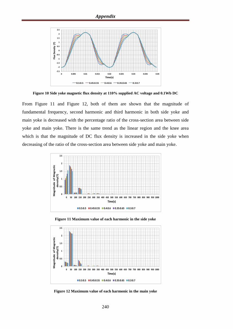
Appendix
240
Figure 10 Side yoke magnetic flux density at 110% supplied AC voltage and 0.1Wb DC
From Figure 11 and Figure 12, both of them are shown that the magnitude of
fundamental frequency, second harmonic and third harmonic in both side yoke and
main yoke is decreased with the percentage ratio of the cross-section area between side
yoke and main yoke. There is the same trend as the linear region and the knee area
which is that the magnitude of DC flux density is increased in the side yoke when
decreasing of the ratio of the cross-section area between side yoke and main yoke.
Figure 11 Maximum value of each harmonic in the side yoke
Figure 12 Maximum value of each harmonic in the main yoke
-2.5
-2
-1.5
-1
-0.5
0
0.5
1
1.5
2
2.5
0 0.005 0.01 0.015 0.02 0.025 0.03 0.035 0.04
Flu
x D
en
sity
(T)
Time(s)
0.5:0.5 0.45:0.55 0.4:0.6 0.35:0.65 0.3:0.7
0
0.5
1
1.5
2
2.5
0 50 100 150 200 250 300 350 400 450 500 550 600 650 700 750 800 850 900 950 1000
Ma
gn
itu
de
of
Ma
gn
eti
c
de
nsi
ty(T
)
Time(s)
0.5:0.5 0.45:0.55 0.4:0.6 0.35:0.65 0.3:0.7
0
0.5
1
1.5
2
2.5
0 50 100 150 200 250 300 350 400 450 500 550 600 650 700 750 800 850 900 950 1000
Ma
gn
itu
de
of
Ma
gn
eti
c
de
nsi
ty(T
)
Time(s)
0.5:0.5 0.45:0.55 0.4:0.6 0.35:0.65 0.3:0.7
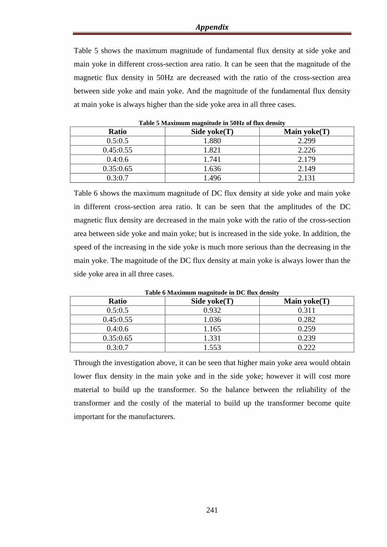
Appendix
241
Table 5 shows the maximum magnitude of fundamental flux density at side yoke and
main yoke in different cross-section area ratio. It can be seen that the magnitude of the
magnetic flux density in 50Hz are decreased with the ratio of the cross-section area
between side yoke and main yoke. And the magnitude of the fundamental flux density
at main yoke is always higher than the side yoke area in all three cases.
Table 5 Maximum magnitude in 50Hz of flux density
Ratio Side yoke(T) Main yoke(T)
0.5:0.5 1.880 2.299
0.45:0.55 1.821 2.226
0.4:0.6 1.741 2.179
0.35:0.65 1.636 2.149
0.3:0.7 1.496 2.131
Table 6 shows the maximum magnitude of DC flux density at side yoke and main yoke
in different cross-section area ratio. It can be seen that the amplitudes of the DC
magnetic flux density are decreased in the main yoke with the ratio of the cross-section
area between side yoke and main yoke; but is increased in the side yoke. In addition, the
speed of the increasing in the side yoke is much more serious than the decreasing in the
main yoke. The magnitude of the DC flux density at main yoke is always lower than the
side yoke area in all three cases.
Table 6 Maximum magnitude in DC flux density
Ratio Side yoke(T) Main yoke(T)
0.5:0.5 0.932 0.311
0.45:0.55 1.036 0.282
0.4:0.6 1.165 0.259
0.35:0.65 1.331 0.239
0.3:0.7 1.553 0.222
Through the investigation above, it can be seen that higher main yoke area would obtain
lower flux density in the main yoke and in the side yoke; however it will cost more
material to build up the transformer. So the balance between the reliability of the
transformer and the costly of the material to build up the transformer become quite
important for the manufacturers.

Appendix
242
3 Cable information
Table 7 Dimension of single core cable
Parameter Value
(mm) Calculation of cable diameter (mm)
Diameter of conductor 21.5 21.5+0=21.5
Thickness of Conductor screen 0.8 21.5+0.8*2=23.1
Thickness of insulation 19.0 23.1+19*2=61.1
Thickness of core screen 1.0 61.1+1.0*2=63.1
Thickness of Semicon WST 1.0 63.1+1.0*2=65.1
Thickness of lead sheath 3.5 65.1+3.5*2=72.1
Thickness of Bitumen 0.5 72.1+0.5*2=73.1
Thickness of MDPE sheath 3.65 73.1+3.65*2=80.4
4 Publication
1. Rui Zhang; T. Byrne; D. Jones; Zhongdong Wang; "A Technical Experience
During Network Asset Replacement: Investigating Cable and Transformer Switching
Interactions," CIRED 2010 Workshop Lyon, France, 7-8 June 2010
2. Rui Zhang; Swee Peng Ang; Haiyu Li; Zhongdong Wang; "Complexity of
ferroresonance phenomena: sensitivity studies from a single-phase system to three-
phase reality," High Voltage Engineering and Application (ICHVE), 2010 International
Conference on vol., no., pp.172-175, 11-14 Oct. 2010
3. Rui Zhang; Haiyu Li; Zhongdong Wang; "Switching Ferroresonant Transient
Study using Finite Element Transformer Model, " 4th Universities High Voltage
Network Conference, 18-19 Jan. 2011
4. Rui Zhang; Jinsheng Peng; Swee.Peng Ang; Haiyu. Li; Zhongdong Wang; Paul
Jarman, “Statistical Analysis of Ferroresonance in a 400 kV Double-Circuit
Transmission System”, IPST 2011, Delft, Netherlands, June 14-17, 2011.
5. C.A. Charalambous; Rui Zhang; Zhongdong. Wang, “Simulating Thermal
Conditions around Core Bolts when Transformer Experiencing Ferroresonance”, IPST
2011, Delft, Netherlands, June 14-17, 2011.