arX

iv:p

hysi

cs/0

2110

03v1

[ph

ysic

s.cl

ass-

ph]

1 N

ov 2

002

ARL Tech. Rep.

Transformation Properties of the Lagrangian

and Eulerian Strain Tensors

Thomas B. Bahder

U. S. Army Research Laboratory

2800 Powder Mill Road

Adelphi, Maryland, USA 20783-1197

(February 20, 2001)

Abstract

A coordinate independent derivation of the Eulerian and Lagrangian strain

tensors of finite deformation theory is given based on the parallel propagator,

the world function, and the displacement vector field as a three-point tensor.

The derivation explicitly shows that the Eulerian and Lagrangian strain ten-

sors are two-point tensors, each a function of both the spatial and material

coordinates. The Eulerian strain is a two-point tensor that transforms as a

second rank tensor under transformation of spatial coordinates and transforms

as a scalar under transformation of the material coordinates. The Lagrangian

strain is a two-point tensor that transforms as scalar under transformation of

spatial coordinates and transforms as a second rank tensor under transforma-

tion of the material coordinates. These transformation properties are needed

when transforming the strain tensors from one frame of reference to another

moving frame.

1

I. BACKGROUND

The U.S. Army is developing an electromagnetic gun (EMG) for battlefield applications.

During the past few years, on a recurring basis, Dr. John Lyons (former ARL Director)

and Dr. W. C. McCorkle (Director of U. S. Army Aviation and Missile Command) have

requested that I look at some of the physics of the EMG. In the most recent request, I was

asked to look at stresses in a rotating cylinder. For the case of an elastic cylinder, this is

a classic problem that is solved in many texts on linear elasticity [1,2,3,4,5,6]. However,

when these derivations are examined closely, one finds certain shortcomings [7]. Therefore,

I spent some time looking at the problem of stresses in elastic rotating cylinders. That work

resulted in a manuscript [7]. In the course of this work [7], I had to clearly understand the

transformation properties of the Largangian and Eulerian strain tensors of finite deformation

theory. I was quite dissatisfied with the standard derivations of the Largangian and Eulerian

strain tensors because these derivations take either of two (both unpalatable) approaches.

In the first approach, shifter tensors are used, which are often defined as inner products

between two basis vectors at two different spatial locations [8,9]. In this approach, basis

vectors are not parallel transported to the same spatial location before the inner product

is carried out. This is unpalatable, even in Euclidean space, unless one is using Cartesian

coordinates. In the second approach, convected (moving) coordinates are used, and vectors

and tensors are associated with a given coordinate in the convected (moving) coordinate

system, rather than being associated with a point in the underlying space.

In the derivation that I present below, I avoid both of the unpalatable features mentioned

above. I provide a coordinate independent derivation of the Lagrangian and Eulerian strain

tensors based on standard concepts in differential geometry: the parallel propagator, the

world function, and the displacement vector field as a three-point tensor.

The derivation that I present below is also useful for gaining a basic understanding of the

role of the unstrained state, or reference configuration, in the definition of the strain tensors.

Having a firm conceptual grasp of the role of the unstrained state in the definition of the

2

strain tensors is imperative for understanding the behaviour of pre-stressed materials under

finite deformations in high-stress applications, such as, for example, in the electromagnetic

rail gun [16].

II. INTRODUCTION

The theory of stresses in rotating cylinders and disks is of great importance in practical

applications such as rotating machinery, turbines and generators, and wherever large rota-

tional speeds are used. In a previous work [7], I gave a detailed treatment of stresses in a

rotating elastic cylinder. This is a classic problem that is treated in many texts on linear

elasticity theory [2,3,4,5,6]. These treatments linearize the strain tensor in gradient of the

displacement field, assuming that these (dimensionless) gradients are small. I point out in

Ref [7] that for large angles of rotation the quadratic terms (in displacement gradient in the

definition of strain) are as large as the linear terms, and consequently, these quadratic terms

cannot be dropped. In Ref [7], I provide an alternative derivation of stresses in an elastic

cylinder that relies on transforming the problem from an inertial frame (where Newton’s

second law is valid) to the co-rotating frame of the cylinder–where the displacements gradi-

ents are small. During the course of that solution, I had to transform the Lagrangian and

Eulerian strain tensors of finite elasticity to the (non-inertial) co-rotating frame of reference

of the cylinder, which is a moving, accelerated frame. This work required the detailed un-

derstanding of the transformation properties of the Lagrangian and Eulerian strain tensors.

The standard derivation of these strain tensors is done with the help of shifter ten-

sors [8,9]. Shifter tensors are often defined in terms of inner products of basis vectors that

are located at two different spatial points [8,9]. For me, inner products between vectors

at two different points is an unpalatable operation, even in Euclidean space. In order to

compute the inner product between two vectors, the vectors must first be parallel trans-

ported to the same spatial point (unless we are using Cartesian coordinates, in which case

the derivation becomes coordinate specific).

3

In other treatments, where shifter tensors are not employed in the derivation of strain

tensors, convected (moving) coordinates are used, see for example [10,11,12,13]. When

using convected (moving) coordinates, the coordinates of the initial undeformed point and

the deformed point are the same, but the basis vectors change during deformation. In

derivations of strain tensors using convected coordinates, vectors and tensors are associated

with a given point in the convected (moving) coordinate system, rather than being associated

with a point in the underlying (inertial) space. Tensors are absolute geometric objects, and

they should properly be associated with a point in the underlying space, and not a given

coordinate, e.g., in moving coordinates.

In this work, I avoid the unpalatable features of the strain tensor derivation mentioned

in the above two paragraphs. I derive the strain tensors using the concept of absolute

tensors, where a tensor is associated with a point in the space–rather than the coordinates

in a given (moving) coordinate system. I provide a coordinate independent derivation of

the Lagrangian and Eulerian strain tensors, where I keep track of the positions of the basis

vectors. The derivation necessarily uses two-point (and three-point) tensors [8,9,14,15]. The

derivation is based on standard concepts in differential geometry: the parallel propagator

(a two-point tensor), the world function (a two-point scalar), and the displacement vector

field (a three-point tensor). This derivation makes clear the transformation properties of

the strain tensors under coordinate transformations from one frame of reference to a second

frame that is moving and accelerated (with respect to the first frame).

The derivation below of the Eulerian and Lagrangian strain tensors makes the trans-

formation properties (e.g., to a moving frame) clear. Furthermore, this derivation makes

the role of the reference (unstrained) configuration more clear in the definition of the strain

tensors. Clarifying this role is of importance for applying finite deformation theory to pre-

stresssed materials, which are capable of withstanding higher-stress applications, such as in

rotating machinery [7,16]. Finally, the derivation presented here allows the generalization

of the definition of strain tensors to the realm where general relativity applies [17,18].

4

III. GEOMETRIC BACKGROUND

In Euclidean space, a vector can be trivially parallel propagated in the sense that after

a round trip the vector still points in the same direction. In Riemannian space, the parallel

displaced vector is not equal to itself after the round trip parallel displacement. In this sense,

in Euclidean space we need not distinguish the position of a vector because “it always points

in the same direction under parallel displacement”–even though its components may be dif-

ferent from point to point because the basis vectors, onto which we project the vector, point

in a different direction from point to point. So, in Euclidean space the parallel displaced

(physical) vector (a geometric object) is thought to point in the same physical direction. In

Riemannian space, however, the situation is quite different. In Riemannian space, when a

vector is parallel displaced it will in general point in a different direction. The physical test

is to parallel displace the vector along a curve that returns to the starting point. If there is

non-zero curvature, as measured by the Riemann curvature tensor, then upon returning to

its starting point the vector components will be different than the initial vector components

at the starting point. So, in Reimannian space, it is imperative to specify the position of a

vector. In Euclidean space, appropriate to material deformations, I also keep track of the

position of a vector. This additional care in Euclidean space, together with the transforma-

tion properties of the world function, leads to a clearer understanding of the transformation

properties of the Lagrangean and Eulerian strain tensors, under transformations from one

system of coordinates to another that is in relative motion (a moving frame).

In this section I briefly review the fundamental geometric quantities that naturally arise

in discussion of deformation, but which are not usually discussed in this context. These

quantities are the world function (or fundamental two-point scalar of the the space), the

parallel propagator, and the position vector. This section will also serve to define my nota-

tion. Each of the quantities mentioned are examples of a class of geometric object objects

known as two-point tensors, which occur naturally in the discussion of deformations. I have

found useful discussions of general tensor calculus in Synge and Schild [19] and Synge [15],

5

and discussions oriented toward deformation theory in the Appendix by Ericksen in Treus-

dell and Toupin [14], and in Narasimhan [9], Eringen [8], and Eringen [20]. In particular,

discussion of two-point tensors can be found in Synge [15], Ericksen [14], Narasimhan [9]

and Eringen [8].

A. The World Function

The world function was initially introduced into tensor calculus by Ruse [21,22],

Synge [23], Yano and Muto [24], and Schouten [25]. It was further developed and extensively

used by Synge in applications to problems dealing with measurement theory in general rela-

tivity [15]. An application of the world function to problems of navigation and time transfer

can be found in Ref. [26]. Compared to the enormous attention given to tensors, the world

function has been used very little by physicists. Yet, when geometry plays a central role,

such as in deformation theory, the world function is helpful to clarify and unify the under-

lying geometric concepts. The world function is simply one-half the square of the distance

between two points in the space. In applications to relativity and 4-dimensional space-time,

the space-time is often taken as a general (curved) pseudo-Riemannian space [15]. In appli-

cations to deformation of materials, we are concerned with a Euclidean three-dimensional

space. However, for understanding the transformation properties of displacement vectors and

strain tensors, it is helpful to use the concept of world function in a Euclidean 3-dimensional

space described by curvilinear coordinates xi, i = 1, 2, 3, with a metric gij, which in general

is a function of position.

Consider two points in a general Riemannian space, P1 and P2, connected by a unique

geodesic path (a straight line in Euclidean space) Γ, given by xi(u), i = 1, 2, 3, where

u1 ≤ u ≤ u2, and xi(u) are curvilinear coordinates of the path. The coordinates of point

P1 = xi1 and point P2 = xi

2. In general, a geodesic is defined by a class of special

parameters u′, u · · ·, that are related to one another by linear transformations u′ = au + b,

where a and b are constants. Here, u is a particular parameter from the class of special

6

parameters that define the geodesic Γ, and xi(u) satisfy the geodesic equations

d2xi

du2+ Γi

jk

dxj

du

dxk

du= 0 (1)

Using Cartesian coordinates zk (rather than general curvilinear coordinates xk) in Euclidean

space, the Christoffel symbol Γijk = 0, and the solution of Eq. (1) is simply

zi(u) = zα1 +u− u1

u2 − u1

(zα2 − zα1 ) (2)

where u1 ≤ u ≤ u2, i = 1, 2, 3 and the Cartesian coordinates of points P1 and P2 are zα1 and

zα2 , respectively. In a general Riemannin space, the world function between point P1 and P2

is defined as the integral along Γ in arbitrary curvilinear coordinates xi by

Ω(P1, P2) =1

2(u2 − u1)

∫ u2

u1

gijdxi

du

dxj

dudu (3)

The value of the world function has a simple geometric meaning: it is one-half the distance

between points P1 and P2. Its value depends only on the eight coordinates of the points

P1 and P2. The value of the world function in Eq. (3) is independent of the particular

special parameter u in the sense that under a transformation from one special parameter u

to another, u′, given by u = au′ + b, with xi(u) = xi(u(u′)), the world function definition in

Eq. (3) has the same form (with u replaced by u′).

The world function is the fundamental two-point invariant that characterizes the space.

It is invariant under independent transformation of coordinates at P1 and at P2. For a given

space, the world function between points P1 and P2 has the same value independent of the

coordinates used, which makes it a useful coordinate independent quantity. In Euclidean

space, using Cartesian coordinates, the world function has the simple form

Ω(zi1, zj2) =

1

2δij ∆zi ∆zj (4)

where δij is the Euclidean metric with only non-zero diagonal components (+1,+1,+1),

and ∆zi = (zi2 − zi1), i = 1, 2, 3, where zi1 and zi2 are the Cartesian coordinates of points

P1 and P2, respectively. (I use the convention that all repeated indices are summed, unless

otherwise stated.)

7

The world function has a number of interesting properties, see Synge [15]. Calcula-

tions of the world function for spaces other than Euclidean spaces, namely four-dimensional

space-time, can be found in Refs. [15,26,27,28,29]. In what follows, I restrict myself to a

three-dimensional space. By transforming to a new system of coordinates, say spherical

coordinates,

x = r cos θ cosφ (5)

y = r cos θ sinφ (6)

z = r cos θ (7)

the world function in Eq. (4) can be expressed as a function of spherical coordinates of point

P1 = (r1, θ1, φ1), and P2 = (r2, θ2, φ2).

Consider a geodesic given by Eq. (1) in a general 3-dimensional Riemannian space. The

covariant derivatives of the world function have two important properties:

∂ Ω(P1, P2)

∂ xi2

= (u2 − u1)

(

gijdxj

du

)

P2

= Lλi2 (8)

∂ Ω(P1, P2)

∂ xi1

= −(u2 − u1)

(

gijdxj

du

)

P1

= −Lλi1 (9)

where

L = [2Ω(P1, P2)]1/2 =

∫ P2

P1

ds =∫ u2

u1

[

gijdxi

du

dxj

du

]1/2

du (10)

is the length of the geodesic between P1 and P2, gij is the metric in coordinates xi, and

λi1 and λi2 are components of the unit tangent vectors at end points P1 and P2 (assuming

non-null geodesics [15]):

λi1 =

(

gijdxj

ds

)

P1

(11)

λi2 =

(

gijdxj

ds

)

P2

(12)

where the relation between parameter u and arc length s is given by Eq. (10). In Eq. (8)

and (9), the covariant partial derivatives with respect to xi1 and xi

2 are done with respect to

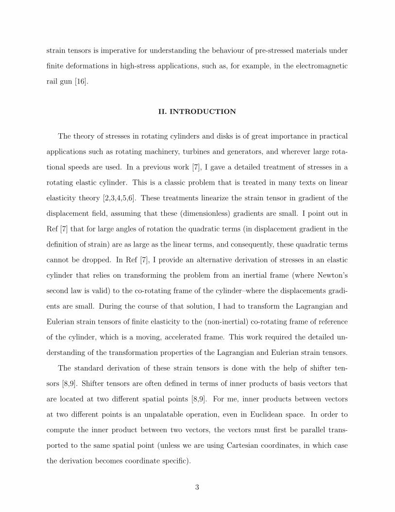
the coordinates of points P1 and P2. See Fig. (1).

8

For the special case of interest in deformation of materials, the space is three-dimensional

Euclidean, the geodesic is a straight line, and the vectors λi1 and λi2 are colinear, although

I still consider them as existing at distinct points. Using Cartesian coordinates and the

explicit form of the world function in Eq. (4), Eq. (8) and (9) take the form

∂ Ω(P1, P2)

∂ zi2= ≡ Ωi2 = δij

(

zj2 − zj1)

= Lλi2 (13)

∂ Ω(P1, P2)

∂ zi1= ≡ Ωi1 = −δij

(

zj2 − zj1)

= −Lλi1 (14)

where I used Synge’s short-hand notation for the components of the covariant partial deriva-

tives by putting subscripts on the indices to indicate which coordinates were differentiated.

This short-hand notation is particularly convenient to show the transformation properties of

the world function and to indicate the spatial location of vectors and tensors. For example,

the quantity Ωi2 transforms as a vector under coordinate transformations at P2 and as a

scalar under coordinate transformations at point P1. The quantity λi2 is a vector located at

point P2. Note that by virtue of their definitions in the left side of Eq. (13) and (14), the

right sides are two-point tensors, whose components are functions of coordinates at point

P1 and P2. For example, the right side of Eq. (14) is a product of a two-point scalar L, and

a one point vector, λi1 at P1.

B. Parallel Propagator

Given a vector with components vi1 at point P1, the vector is said to be parallel prop-

agated from P1 to P2 along a geodesic curve C specified by xi(u), u1 ≤ u ≤ u2, where

P1 = xi(u1) and P2 = xi(u2), when its covariant derivative is zero along this curve:

dvi

du+ Γi

jk vj dx

k

du= 0 (15)

Equation (15) is a mapping: given the components of a vector, vi1 at point P1, we obtain

the components vi2 of the parallel transported vector at point P2 by solving Eq. (15). It

is convenient to define a two-point tensor, gi2j1, called the parallel propagator [15], which

9

gives the components of a vector under parallel translation of the vector from point P1 to

point P2. Given a vector with components vi1 at point P1, the propagator gi2j1 relates the

components of this vector at P1 to the components vi2 of this same vector after parallel

translation to point P2

vi2 = gi2i1 vi1 (16)

In a general Riemannian space, the components of the vector at point P2 depend on the

path of parallel translation from P1 to P2, in the sense that the path must be a geodesic by

the definition of the parallel propagator. However, in Euclidean space these components are

completely path independent; the components depend only on the end points P1 and P2.

A vector is considered as a geometric object, which means that it is independent of

coordinate system. In a Riemannian space, under the operation of parallel propagation a

vector changes in such a way that its magnitude stays the same but its absolute direction can

change because of the curvature of the space [30]. The direction of the parallel propagated

vector is of course referred to the local basis vectors. That the vector direction changes under

parallel translation can be understood by taking a vector at point P and parallel translating

it over a curve that returns to point P . When compared at point P , the components of the

initial vector and the round-trip-parallel-transported vector will (in general) be different. It

is in this sense that a vector changes its direction under parallel transport.

As mentioned above, the change in the vector that results under parallel transport de-

pends on the path of parallel propagation (a geodesic). Two vectors that are parallel prop-

agated along the same path will maintain the angle between them along the path.

In a Euclidean space, a vector (the geometric object) is considered to be unchanged when

parallel propagated. The only thing that happens is that the components of the vector on

the local basis must change according to what is required to keep the vector “pointing in

the in same direction”.

In Euclidean space, the parallel propagator in Cartesian coordinates is trivial–its com-

ponents are just the components of a delta function. The components of a vector at point

10

P1 are related to the components of the same vector parallel translated to point P2 by the

propagator (whose components are given in a Cartesian coordinate basis):

δi2j1 =

+1 i = j

0 i 6= j(17)

Equation (17) agrees with our notion from elementary geometry that in Cartesian coordi-

nates the vector components are constant under parallel propagation. However, using the

parallel propagator in Cartesian coordinates, I can, for example, compute the propagator

gi2j1 in curvilinear coordinates xi = (r, θ, φ) given in Eq. (5)–(7), by the two-point tensor

transformation rule

gi2j1 =∂ xi(P2)

∂ zm∂ zn(P1)

∂ xjδm2

n1(18)

The parallel propagator gi2j1 is a two-point tensor because it transforms as a vector under

coordinate transformation at point P1 and under coordinate transformation at point P2.

In Cartesian coordinates, when the points are made to coincide, P2 → P1, the propagator

reduces to a Kronecker delta at point P1: δm2

n1→ δmn(P1). In general curvilinear coordi-

nates, when the points P1 and P2 coincide, the parallel propagator reduces to the mixed

components of the mertic tensor gi2j1:

limP2→P1

gi2j1 → gij(P1) (metric at P1) (19)

The mixed components of the metric tensor at P1, gij(P1) ≡ gik(P1) gkj(P1), are a Kronecker

delta–a unit tensor whose components are the same in all systems of coordinates. Indices

can be lowered on two-point tensors using the appropriate metric. For example, the index i

of the propagator gi2j1 can be lowered by using the metric tensor at point P2:

gk2j1 = gki(P2) gi2j1 (20)

When the points are made to coincide, P2 → P1, the covariant components of the propagator

becomes the covariant components of the metric tensor at P1, gk2j1 → gkj(P1), where gkj(P1)

is the metric at P1.

11

The covariant derivatives of the world function Ω(P1, P2) between points P1 and P2 are

related to the parallel propagator by [15]

Ωi1j1 = gi1j1 (metric at P1) (21)

Ωi1j2 = Ωj2i1 = −gi1j2 = −gj2i1 (parallel propagator) (22)

Ωi2j2 = gi2j2 (metric at P2) (23)

Other useful properties of the parallel propagator are discussed by Synge [15].

C. Position Vector

The position vector occupies a central role in deformation theory. For this reason, I

discuss it in detail below. In elementary geometry, a point P can be identified by its position

vector r, which can be specified in Euclidean-space Cartesian coordinates as

r = zn in (24)

where zn are the Cartesian components of the vector r and also the Cartesian coordinates

of the point P . In terms of general coordinate basis vectors en = ∂/∂xn associated with the

curvilinear coordinates xn, the vector r is given by

r = zn Amn(P ) em(P ) = ζm em(P ) (25)

The position vector is a geometric object at point P . Among all basis vectors, the Cartesian

basis vectors in are unique in that they are usually not associated with a particular spatial

point. However, when we express these Cartesian basis vectors in terms of curvilinear basis

vectors en, then we must imagine that these basis vectors exist at a particular point P .

Hence, the transformation between the Cartesian basis vector im and curvilinear coordinate

basis vectors em at point P associated with coordinates xi is given by

in(P ) = Amn(P ) em(P ) (26)

where the matrix Amn (P ) depends on the coordinates of point P :

12

Amn(P ) =

∂ xm

∂ zn(P ) (27)

In Cartesian coordinates, the components of the vector r are simply the Cartesian co-

ordinates zn of point P . The three numbers (z1, z2, z3) transform as the components of a

vector under orthogonal coordinate transformations. Note that in curvilinear coordinates,

the components of the position vector, ζm, are not the curvilinear coordinates of point P .

Also, note that the position vector r of point P has a magnitude equal to the Euclidean

length from the origin of coordinates, say point O, to point P . The position vector of point

P is a geometric object at point P , however, it also depends on the point O. This depen-

dence on point O is coordinate independent. Therefore, the position vector of point P is a

two-point tensor; it depends on point P and on point O. The transformation properties of

the position vector are that of a scalar when a change of coordinates is made at point O and

the transformation is that of a vector when coordinates at point P are changed.

In a Riemannian (a generalization of Euclidean space) space, the components of the

position vector ri(P ) at point P can be defined in terms of the covariant derivative of the

world function

riP =∂ Ω(O,P )

∂ ziP≡ ΩiP (O,P ) = [2ΩiP (O,P )]1/2 ri(P ) (28)

where riP is a unit vector at point P and [2 ΩiP (O,P )]1/2 is the length of the geodesic from

point O to point P . For the case of Euclidean space, [2 ΩiP (O,P )]1/2 is the length of the

straight line OP . Equation (28) shows explicitly that the position vector, riP , is a two-point

tensor.

D. Displacement Vector

Consider an elastic body that undergoes a finite deformation in time. The deformation

can be specified by a flow function or displacement mapping function

zk = zk(Zm, t) (29)

13

where the coordinates zk (here taken to be Cartesian) of a particle at point Q at time

t are given in terms of the particle’s coordinates Zk of point P in some reference state

(configuration) at time t = to, so that zk(Zm, to) = Zk. I assume the deformation mapping

function has an inverse, which I quote here for later reference

Zm = Zm(zk, t) (30)

I assume that both the coordinates zk and Zm refer to the same Cartesian coordinate

system [33].

In deformation theory, the initial position of the particle in the medium at point P is

specified by a vector

R(P ) = Zmk ik(P ) (31)

and the final position is specified by a position vector

r(Q) = zk ik(Q) (32)

where the quantities ik(P ) and ik(Q) are the Cartesian basis vectors at point P and point

Q, respectively. Conventionally, the deformation of a medium is described by specifying the

displacement “vector field”, which is defined as a difference of these two position vectors.

However, the basis vectors ik(P ) and ik(Q) are at different points in the space. Since vectors

can be subtracted only if they are at the same point, I must parallel translate ik(P ) to point

Q, or, parallel translate ik(Q) to point P . Depending on which mapping I choose, I arrive

at the Eulerian or the Lagrangian displacement vector.

First, I parallel translate vector R(P ) to point Q, and then subtract the vectors at point

Q, see Fig. (2). This procedure defines the components of the Eulerian displacement vector

at point Q:

u(Q) = r(Q)−R(Q) (33)

This Eulerian displacement vector in Eq. (33) is often called the displacement vector in

the spatial representation [8,9,31]. Alternatively, I can parallel translate the vector r(Q) to

14

point P , and then subtract the vectors at point P . This procedure defines the Lagrangian

displacement vector at point P :

U(P ) = r(P )−R(P ) (34)

This Lagrangian displacement vector in Eq. (34) is often called the displacement vector in

the material representation [8,9,31]. Equations (33) and (34) show that these two vectors

are actually referred to basis vectors at different points. In fact, the two vectors u(Q)

and U(P ) are related by parallel translation. In a Euclidean space, these vectors are the

same geometric objects but they are expressed in terms of basis vectors located at different

positions

In order to further clarify the transformation properties of these two displacement vec-

tors, I use the position vector as discussed in the previous section. Consider the deformation

mapping function in curvilinear coordinates, xk(Xm, t). This function specifies the coordi-

nates xk (point Q) of a particle at current time t in terms of the coordinates Xk (point P )

of the particle in the reference configuration at time t = to, so that

xk(Xm, to) = Xk (35)

In addition, there exists a straight line (a geodesic) Γ connecting the points P and Q.

The covariant components of the position vector of point P , R(P ) = Rnen(P ), in

curvilinear coordinates xi are given by (see Eq. (28))

RiP =∂ Ω(O,P )

∂ xiP

≡ ΩiP (O,P ) = [2 Ω(O,P )]1/2 RiP (36)

where RiP are the components of the unit vector at point P tangent to Γ that connects

point P and Q. Similarly, the covariant components of vector r(Q) = rn en(Q) in curvilinear

coordinates xi are given by

riQ =∂ Ω(O,Q)

∂ xiQ

≡ ΩiQ(O,Q) = [2Ω(O,Q)]1/2 riQ (37)

where riQ are the components of the unit vector at point Q tangent to Γ. From Eq. (36)

and (37) it is clear that both RiP and riQ are two-point tensor objects. The quantity RiP

15

depends on point O and P and transforms as a vector under coordinate transformations at

P and as a scalar under coordinate transformations at point O. The quantity riQ transforms

as a vector under coordinate transformations at point Q and as a scalar under coordinate

transformations at point O.

The components of the Eulerian displacement vector in Eq. (33) (at point Q) are defined

in terms of the components of RiP parallel translated to point Q:

RiQ = giQjP RjP (38)

= giQjP

ΩjP (O,P ) (39)

where ΩjP (O,P ) = gjk(P ) ΩkP (O,P ), and gjk(P ) is the metric at point P in coordinates xi.

The contravariant components of the Eulerian displacement vector in Eq. (33) are given by

uiQ = ΩiQ(O,Q)− giQjP

ΩjP (O,P ) (40)

Similarly, the components of the Lagrangian displacement vector are given by

U iP = giPjQ ΩjQ(O,Q)− ΩiP (O,P ) (41)

The vectors whose components are U iP and uiQ, are related by parallel transport along the

geodesic Γ connecting P and Q (not along the particle displacement line given by Eq.(29)).

Transporting U iP to point Q

U iQ = giQkP

UkP (42)

= giQjP

[

gjPkQ ΩkQ(O,Q)− ΩjP (O,P )]

(43)

= δik(Q)ΩkQ(O,Q)− giQjP

ΩjP (O,P ) (44)

= uiQ (45)

where in the transition from Eq. (43) to (44) I have used the identity satisfied by the parallel

propagator:

δik(Q) = giQjP gjPkQ (46)

16

where δik(Q) is a unit tensor (delta function) at point Q. Equation (46) is the statement

that parallel propagation of a vector has an inverse, so the result that U i(P ) and ui(Q) are

related by parallel transport is true in both Euclidean and Reimannian spaces.

IV. STRAIN TENSORS

At time t = to, consider two particles in the medium that are at positions P1 and P2,

respectively, and are separated by a finite distance ∆S = [2Ω(P1, P2)]1/2. At a later time

t > to these particles have moved to new positions Q1 and Q2 and are separated by a distance

∆s = [2Ω(Q1, Q2)]1/2, see Fig. (3).

As a measure of strain, I take the 4-point scalar

Ψ(P1, P2;Q1, Q2) ≡ (∆s)2 − (∆S)2 = 2Ω(Q1, Q2)− 2Ω(P1, P2) (47)

Note that Ψ(P1, P2;Q1, Q2) depends on four points P1, P2, Q1, and Q2, and by virtue of

its definition in terms of the world function, Ψ is a true four-point scalar invariant under

separate coordinate transformations at each of these four points. In Cartesian coordinates,

Eq. (47) becomes

Ψ(zi1, zi2;Z

j1, Z

j2) = δij (z

i1 − zi2) (z

j1 − zj2))− δij (Z

i1 − Z i

2) (Zj1 − Zj

2)) (48)

where zi1 = zi(Zm1 , t) and zi2 = zi(Zm

2 , t) and they are related to the reference configuration

at t = to by

zi(Zm1 , to) = Z i

1 (49)

and

zi(Zm2 , to) = Z i

2 (50)

and zi(Zm, t) is the deformation mapping function in Cartesian coordinates, given in

Eq. (29). If I consider the particle positions P1 and P2 as separated by an infinitesimal

distance, then, by assuming continuity in the medium and a finite time t − to, the points

17

Q1 and Q2 are also infinitesimally separated. However, because t− to is finite, the distance

between P1 and Q1 is finite (not infinitesimal). Expanding Eq. (50) about the initial position

of the first particle

zi2 = zi(Zk1 , t) +

∂ zi

∂ Zj(Zm

1 , t) (Zj2 − Zj

1) + · · · (51)

using zi1 = zi(Zk1 , t), leads to the relation between spatial (Eulerian) coordinates zi and

material (Lagrangian) coordinates Zk

∆zi =∂ zi

∂ Zj(Zm

1 , t)∆Zj + · · · (52)

where ∆zi = zi2 − zi1 and ∆Z i = Z i2 − Z i

1. Using Eq. (52) in Eq. (48) leads to the measure

of strain in Cartesian coordinates

(∆s)2 − (∆S)2 =

(

δij∂ zi

∂ Zm

∂ zi

∂ Zn− δmn

)

∆Zm ∆Zn + · · · (53)

= 2Emn ∆Zm∆Zn + · · · (54)

where the quantity in parenthesis is the Lagrangean strain tensor, Emn. The higher order

terms in ∆Zm are small because I can always choose the two initial points P1 and P2

arbitrarily close together. From Eq. (53)–(54), it is clear that the Lagrangean strain tensor

is a two-point tensor, depending on initial point P (in the reference configuration at t = to)

and point Q (at time t). Note that in Eq. (54) there is no restriction to short times t− to,

since I can always choose ∆Zn sufficiently small.

The Eullerian tensor can be obtained from Eq. (54) by using the fact that the flow

function in Eq. (29) has an inverse. Using

∆Zn =∂Zn

∂zi(zi, t)∆zi (55)

I get the measure of strain in terms of the Eulerian strain tensor emn:

(∆s)2 − (∆S)2 =

(

δmn − δkl∂ Zk

∂ zm∂ Z l

∂ zn

)

∆zm ∆zn + · · · (56)

= 2 emn∆zm ∆zn + · · · (57)

18

A. Strain Tensor Derivation in Curvilinear Coordinates

I return to the definition of the measure of strain given in Eq. (47). In the reference

configuration at t = to, consider two particles at points P1 and P2 with curvilinear coordi-

nates X1 and X2. At a later time t, these two particles are at positions Q1 and Q2 with

curvilinear coordinates x1 and x2, respectively. Consider the first term on the right side of

Eq. (47), which is an integral along a straight line Q1Q2:

Ω(Q1, Q2) =1

2(w2 − w1)

∫ w2

w1

gijUi U j dw (58)

where U i = dxi(w)/dw and where the geodesic (straight line) is parametrized by xi(w), with

w1 ≤ w ≤ w2 and the end points are given by x1 = xi(w1) and x2 = xi(w2), see Fig. 3.

The function xi(w) is a solution of the geodesic Eq. (1). In the case of Eulidean space, and

assuming points P1 and P2 are arbitrarily close, the geodesic in Eq. (58) is a straight line

given by

xi(w) = xi1 +

w − w1

w2 − w1

(xi2 − xi

1) (59)

The flow function in Eq. (29) maps the points P1 and P2 into the points Q1 and Q2. The

points Q1 and Q2 depend on time t. With reasonable continuity assumptions, and the

straight line given in Eq. (59) with U iQ = k(xi2 − xi

1) = k∆xi and k = (w2 − w1)−1, the

world function in Eq. (58) can be approximated by

Ω(Q1, Q2) =1

2(w2 − w1) gij(Q1) k∆xi k∆xj

∫ w2

w1

dw (60)

=1

2gij(Q1)∆xi ∆xj (61)

Similarly, the second term on the right side of Eq. (47) can be approximated as

Ω(P1, P2) =1

2gij(P1)∆X i ∆Xj (62)

where the coordinates X i are the undeformed ones and ∆X i = X i2 − X i

1. The measure of

strain in Eq. (47) is then

19

(∆s)2 − (∆S)2 = gij(Q)∆xi ∆xj − gij(P )∆X i ∆Xj (63)

or using the flow function in Eq. (29),

(∆s)2 − (∆S)2 =

(

gij(Q)∂xi

∂Xk(P,Q)

∂xj

∂X l(P,Q)− gkl(P )

)

∆Xk ∆X l (64)

Note that xi andX i refer to to the same system of coordinates. I have dropped the subscripts

on Q and P since Q1 and Q2, and P1 and P2, are infinitesimally close, respectively. The

quantity in parenthesis on the right side of Eq. (64) is twice the Lagrangian strain tensor:

2EkP lP = gij(Q)∂xi

∂Xk(P,Q)

∂xj

∂X l(P,Q) − gkl(P ) (65)

From Eq. (65), it is clear that the Lagrangian strain tensor is a two-point tensor. Under

transformation of coordinates at point P , EkP lP is a second rank tensor, while under trans-

formation of coordinates at point Q, it is a scalar. The deformation gradient, ∂xi/∂Xk, is

itself a two-point tensor, as can be seen by its transformation property when coordinates at

P and Q are changed.

It is interesting to note that the Lagrangian strain tensor Ekl is conventionally thought to

be a function of material coordinates, X i, which coincide with the point P (in the reference

configuration) [8,9]. The tensor EkP lP can be taken to be a function of only the material

coordinates by using the flow mapping function in Eq. (29), which provides a mapping

between all points P and their images, points Q, under the deformation. I do not pursue

this interpretation below.

The first term in Eq. (65) is the Green deformation tensor:

Ckl = gij(Q)∂xi

∂Xk(P,Q)

∂xj

∂X l(P,Q) (66)

The point P is in the reference configuration at time t = to and the point Q is in the

deformed state at time t. In Eq. (66), the Green deformation tensor is naturally a second

rank tensor with respect to material coordinate transformations (point P ) and it is a scalar

spatial coordinate transformations (point Q). However, the Green tensor is conventionally

20

taken [8,9] as a function of material coordinates by using the flow mapping function in

Eq. (29).

Returning to Eq. (64), and using the flow mapping function in Eq. (29), we can obtain

(∆s)2 − (∆S)2 =

(

gij(Q)− gkl(P )∂Xk

∂xi(P,Q)

∂X l

∂xj(P,Q)

)

∆xi ∆xj (67)

where the Eulerian strain tensor eiQjQ is given by

2 eiQjQ = gij(Q)− gkl(P )∂Xk

∂xi(P )

∂X l

∂xj(P ) (68)

The Eulerian strain tensor eiQjQ is a two-point tensor that is second rank with respect to

spatial coordinates at point Q and is a scalar with respect to material coordinates at point P

. Once again, however, using the flow mapping function in Eq. (29), eiQjQ can be imagined

to depend on the material coordinates xi (point Q) of the deformed state.

V. STRAIN TENSORS IN TERMS OF THE DISPLACEMENT FIELD

The Eulerian and Lagrangian strain tensors can be expressed in terms of the displacement

fields uiQ and U iP in Eq. (40) and (41). In terms of covariant components, the displacement

field vector at Q is given by

uiQ = ΩiQ(O,Q)− giQjP ΩjP (O,P ) (69)

The covariant derivative of uiQ with respect to point Q (coordinates xk) is

uiQ;kQ = ΩiQkQ(O,Q)− g jPiQ

ΩjP lP (O,P )∂X l

∂xk(70)

where I used the chain rule for covariant differentiation since Ω(O,P ) = Ω(O,P (X)) and

the material coordinates X l = X l(xk) are functions of the spatial coordinates xk. It is

clear that the chain rule must be used in Eq. (70) by considering Cartesian coordinates. In

Eq. (70), I also used the fact that in Euclidean space the parallel propagator is a constant

under covariant differentiation. The notation ΩiQkQ(O,Q) means the (i, k) component of

21

the second covariant derivative of the world function at point Q. In Euclidean space, these

second covariant derivatives are simply related to the parallel propagator, see Eq. (21)–(23).

Using Eq. (23), the covariant derivative of the displacement field in Eq. (70) becomes

uiQ;kQ = gik(Q)− g jPiQ

gjl(P )∂X l

∂xk(71)

= gik(Q)− giQlP

∂X l

∂xk(72)

where in the last line the metric at P , gjl(P ), was used to lower the index on the propagator.

Now I multiply Eq. (72) by the parallel propagator gmP iQ, sum on iQ, and solve for the inverse

displacement gradient

∂Xm

∂xk= gmP

kQ− gmP iQ uiQ;kQ (73)

From Eq. (73), it is clear that in Euclidean space, the deformation gradient ∂Xm/∂xk is

simply related to the covariant derivative of the displacement field, uiQ;kQ. Note however,

that in a Riemannian space, for finite deformations, it is generally not possible to solve for

the deformation gradient [18]. Now, using Eq. (73) in Eq. (67), I find the expression relating

the two-point Eulerian strain tensor eiQjQ = eiQjQ(P,Q) to the covariant derivatives of the

three-point displacement field

(∆s)2 − (∆S)2 =[

uiQ;jQ + ujQ;iQ − gkl(Q) ukQ;iQ ulQ;jQ

]

∆xi ∆xj (74)

= 2 eiQjQ ∆xi ∆xj (75)

where

eiQjQ =1

2

[

uiQ;jQ + ujQ;iQ − gkl(Q) ukQ;iQ ulQ;jQ

]

(76)

Equation (76) explicitly shows that the Eulerian strain tensor eiQjQ is a function of two

points, material coordinates at point P and spatial coordinates at point Q. Note that eiQjQ

is not a function of point O, since by Eq. (71) the covariant derivative uiQ;jQ does not depend

on point O. From Eq. (76) it is also clear that eiQjQ transforms as a second rank tensor

22

under spatial coordinate transformations and that it transforms as a scalar under material

coordinate transformations.

An analogous relation can be obtained for the Lagrangian strain tensor by considering

the covariant derivative of the displacement field

UiP ;kP = gjQ

iPΩjQlQ(O,Q)

∂xl

∂Xk− ΩiP kP (O,P ) (77)

Using the relations between the second covariant derivatives of the world function and

propagator in Eq. (21)–(23), and solving for the displacement gradient I get

∂xm

∂Xk= g

mQ

kP− gmQiP UiP ;kP (78)

Inserting the displacement gradient in Eq. (78) into Eq. (64) gives an expression for the

Lagrangian strain tensor EmP nP= EmP nP

(P,Q),

(∆s)2 − (∆S)2 =[

UmP ;nP+ UnP ;mP

+ gij(P )UiP ;mPUjP ;nP

]

∆Xm∆Xn (79)

= 2EmPnP∆X i ∆Xj (80)

where

EmPnP=

1

2

[

UmP ;nP+ UnP ;mP

+ gij(P )UiP ;mPUjP ;nP

]

(81)

Equation (79) shows that the Lagrangian strain tensor EmPnPis a function of the material

coordinates at point P and spatial coordinates at point Q. The Lagrangian strain tensor

transforms as a scalar under spatial coordinate transformations at point Q and as a second

rank tensor with respect to material coordinate transformations at point P . Note that there

are minus sign differences in Eq. (76) and (81). Finally, comparing Eq. (74) and (79), we

have the well-known relation between the two strain tesnors

EmP nP= eiQjQ

∂xi

∂Xm

∂xj

∂Xn(82)

Equation (82) provides a complicated relation between the two two-point strain tensors.

While the displacement fields uiQ and U iP are related to each other by parallel transport,

see Eq. (40)–(41), the strain tensors EmPnPand eiQjQ are related by two-point deformation

gradient tensors, ∂xi/∂Xm, in Eq. (82).

23

VI. SUMMARY

Conventionally, the Eulerian and Lagrangian strain tensors are derived either by using

shifter tensors or by using convected (moving) coordinates. The definition of the shifter

tensor makes use of a scalar product between vectors at two different points in space (without

first parallel translating one vector to the position of the other). When convected coodinates

are used, vectors and tensors are associated with given coordinates in the convected system

of coordinates, rather than being associated with a gven point in the underlying space. As

discussed in the introduction, both of these features are undesireable, when we need to

understand the transformation properties of the strain tensors from an inertial frame to a

moving frame. These transformation properties are also needed in order to generalize the

strain tensor to Riemannian geometry for applications to general relativity.

I have provided a derivation of the Eulerian and Lagrangian strain tensors for finite de-

formations using the concepts of parallel propagator, the world function of J. L. Synge and

the three-point displacement vector field. This derivation avoids the undesireable features

mentioned above. The derivation shows that the Eulerian strain tensor is a two-point object

that transforms as a scalar under transformation of material coordinates and as a second

rank tensor under transformation of spatial coordinates. The derivation also shows that the

Lagrangian strain tensor behaves as a scalar under transformation of spatial coordinates

and as a second rank tensor under transformation of material coordinates. These trans-

formation properties are useful in understanding how these strain tensors transform from

one frame of reference to another moving, non-inertial frame. The formulation presented

here of the transformation properties of these tensors is also useful for understand the role

of the reference (unstrained) configurartion in pre-stressed materials, as discussed in the

introduction.

24

ACKNOWLEDGMENTS

The author thanks Dr. W. C. McCorkle, U. S. Army Aviation and Missile Command,

for suggesting investigation of the problem of stresses in a rotating cylinder, which relied on

the ideas in this manuscript as a conceptual foundation.

25

REFERENCES

[1] A. E. H. Love, p. 148, A Treatise on the Mathematical Theory of Elasticity, Dover Publi-

cations, 4th Edition, New York, (1944).

[2] L. D. Landau and E. M. Lifshitz, p. 22, Theory of Elasticity, Pergamon Press, New York

(1970).

[3] A. Nadai, “Theory of Flow and Fracture of Solids”, p. 487, McGraw-Hill, New York

(1950).

[4] E. E. Sechler, p. 164, Elasticity in Engineering, John Wiley & Sons, Inc., New York (1952).

[5] S. P. Timoshenko and J. N. Goodier, p. 81, Theory of Elasticity, 3rd Edition, McGraw-Hill

Book Company, New York, (1970).

[6] E. Volterra and J. H. Gaines, p. 156, Advanced Strength of Materials, Prentice-Hall, Inc.,

Englewood Cliffs, N.J., USA, (1971).

[7] T. B. Bahder, “Stress in Rotating Disks and Cylinders”, submitted for publication in

Journal of Elasticity.

[8] A. C. Eringen, Nonlinear Theory of Continuous Media, McGraw-Hill Book Company,

New York, (1962).

[9] M. N. L. Narasimhan, Principles of Continuum Mechanics, John Wiley & Sons, Inc., New

York (1992).

[10] F. D. Murnaghan, American Journ. Math., “Finite Deformations of an Elastic Solid”, 59,

235-260 (1937).

[11] A. E. Green and W. Zerna, Theoretical Elasticity, Oxford (1954).

[12] I. S. Sokolnokoff, Tensor Analysis: Theory and Applications to Geometry and Mechanics

of Continua, Second Edition, John Wiley & Sons, Inc., New York (1964).

26

[13] W. Flugge, Tensor Analysis and Continuum Mechanics, Springer-Verlag, New York

(1972).

[14] J. L. Ericksen, “Tensor Fields”, in Appendix of C. Truesdell and R. Toupin “The Classi-

cal Field Theories”, in “Handbuch der Physik”, vol. III, Part 1, Springer-Verlag, Berlin

(1960).

[15] J. L. Synge, Relativity: The General Theory (North-Holland Publishing Co., New York,

1960).

[16] For example, see p. 364 of W. C. McCorkle, “Compensated Pulsed Alternators to Power

Electromagnetic Railguns”, 12th IEEE International Pulsed Power Conference 1999, p.

364–368, vol. I (1999).

[17] G. A. Maugin, “Harmonic Oscillations of Elastic Continua and Detection of Gravitational

Waves”, Gen. Rel. Grav. 3, 241-272 (1973).

[18] J. M. BGambi, A. San Miguel, and F. Vicente, Gen. Rel. Grav., “The Relative Deforma-

tion Tensor for Small Displacements in General Relativity”, 21, 279-286 (1989).

[19] J. L. Synge and A. Schild, Tensor Calculus, Dover Publications, New York (1949).

[20] See A. C. Eringen, in Continuum Physics, Edited by A. C. Eringen, Academic Press, New

York (1971).

[21] H. S. Ruse, “Taylor’s Theorem in the Tensor Calculus”, Proc. London Math. Soc. 32,

87-92 (1931).

[22] H. S. Ruse, “An absolute Partial Differential Calculus”, Quart. J. Math. Oxford Ser. 2,

190 (1931).

[23] J. L. Synge, “A Characteristic Function in Riemannian Space and its Application to the

Solution of geodesic triangles”, Proc. London Math. Soc. 32, 241-258 (1931).

[24] K. Yano and Y. Muto, “Notes on the deviation of geodesics and the fundamental scalar

27

in a Riemannian space”, Proc. Phys.-Math. Soc. Jap. 18, 142 (1936).

[25] J. A. Schouten, “Ricci-Calculus. An Introduction to Tensor Analysis and Its Geometrical

Applications” (Springer-Verlag, 2nd edition, 1954).

[26] T. B. Bahder, “Navigation in curved space-time”, submitted to Am. J. Physics.

[27] R. W. John, “Zur Berechnung des geodatischen Abstands und assoziierter Invarianten im

relativistischen Gravitationsfeld”, Ann. der Phys. Lpz. 41, 67-80, (1984).

[28] R. W. John, “The world function of space-time: some explicit exact results for specific

metrics”, Ann. der Phys. Lpz. 41, 58-70, (1989).

[29] H. A. Buchdahl and N. P. Warner, “On the world function of the Schwarzschild field”,

Gen. Rel. and Grav. 10, 911-923(1979).

[30] J. Kraus, Int. J. Theor. Phys. 12, 35 (1975).

[31] A. J. M. Spencer, p. 63, Continuum Mechanics, Longman Mathematical Texts, Longman,

New York (1980).

[32] J. M. Gambi, P. Romero, A. San Miguel, and F. Vicente, “Fermi coordinate transfor-

mation under baseline change in relativistic celestial mechanics”, International J. Theor.

Phys.30, 1097-1116 (1991).

[33] I use the notation zk and Zk for the Cartesian coordinates and also for the deformation

mapping functions. There is no chance of confusing these two since the context makes it

clear which one is usedin a given instant.

28

FIGURES

P2

P1

λi2

λi1

Figure 1

FIG. 1. A geodesic path is shown in 3-dimensions, with tangent unit vector at the ends.

29

P

Q

O

R(P)

R(Q)U(P)= r(P) − R(P)

u(Q)= r(Q) − R(Q)

r(Q)

r(P)

zk = zk(Zm ,t)

Figure 2

30

FIG. 2. The initial and final position vectors, R(P ) and r(Q), respectively, are shown as well

as their respective parallel translated vectors, R(P ) and r(Q). Also, shown by a solid curve is the

actual displacement path of a representative particle of the medium, labeled by zk = zk(Zm, t).

The dashed straight line is the line (geodesic) connecting the initial and final particle positions.

The Eulerian displacement vector is u = r(Q) − R(Q), which is the difference of two position

vectors at point Q. The Lagrangean displacement vector, U = r(P ) −R(P ), is the difference of

two position vectors at point P .

31

P1

Q1 Q

2

P2

∆s

∆St = to

t > to

Figure 3FIG. 3. The position P1 and P2 of two particles is shown in the reference configuration at

t = to, and the positions Q1 and Q2 of the same two particles is shown at later time t > to. The

path of the particles is shown in solid lines and their displacement is shown in dashed lines.

32