Traitement d'antenne tensoriel - Accueil - TEL

HAL Id: tel-01691607https://tel.archives-ouvertes.fr/tel-01691607v2

Submitted on 22 Jan 2018

HAL is a multi-disciplinary open accessarchive for the deposit and dissemination of sci-entific research documents, whether they are pub-lished or not. The documents may come fromteaching and research institutions in France orabroad, or from public or private research centers.

L’archive ouverte pluridisciplinaire HAL, estdestinée au dépôt et à la diffusion de documentsscientifiques de niveau recherche, publiés ou non,émanant des établissements d’enseignement et derecherche français ou étrangers, des laboratoirespublics ou privés.

Traitement d’antenne tensorielFrancesca Raimondi

To cite this version:Francesca Raimondi. Traitement d’antenne tensoriel. Traitement du signal et de l’image [eess.SP].Université Grenoble Alpes, 2017. Français. NNT : 2017GREAT043. tel-01691607v2

https://tel.archives-ouvertes.fr/tel-01691607v2

https://hal.archives-ouvertes.fr

THESEPour obtenir le grade de

DOCTEUR DE LA COMMUNAUTEUNIVERSITE GRENOBLE ALPESSpecialite : SIGNAL IMAGE PAROLE TELECOMS

Arrete ministeriel : 25 mai 2016

Presentee par

Francesca Elisa Diletta RAIMONDI

These dirigee par Pierre COMON, CNRS

preparee au sein duLaboratoire Grenoble Images Parole Signal Automatique

dans l’Ecole Doctorale Electronique, Electrotechnique,Automatique, Traitement du Signal (EEATS)

Traitement d’antenne tensoriel

These soutenue publiquement le 22 septembre 2017,devant le jury compose de:

M. Olivier J. MichelProfesseur des universites, GIPSA-lab,President du jury

M. Pascal ChevalierProfesseur du CNAM, Chaire d’Electronique(Conservatoire National des Arts et Metiers), Rapporteur

M. Martin HaardtProfesseur des universites, Ilmenau University of Technology,Rapporteur

M. David BrieProfesseur des universites, CRAN(Centre de Recherche en Automatique de Nancy), Examinateur

M. Pierre COMONDirecteur de recherche, GIPSA-lab, CNRS,Directeur de these

Tensor Array Processing

Francesca Elisa Diletta RAIMONDI

A thesis submitted for the degree of

Doctor of Philosophyin Signal Processing

Supervised by Pierre Comon

GRENOBLE ALPS UNIVERSITY

GIPSA-lab, CNRS

September 22, 2017

Thesis Committee:

Chair : Olivier J. MICHEL - GIPSA-labReviewers : Pascal CHEVALIER - CNAM

Martin HAARDT - Ilmenau University of TechnologyExaminer : David BRIE - CRANThesis advisor : Pierre COMON - GIPSA-lab

Acknowledgments

A PhD is the outcome of several contributions (beside the endeavour and the efforts ofthe bewildered student), and I like to interpret it as a Bildungsroman. I am now threeyears older, hopefully wiser, and a grown up researcher.

First, a PhD work, as solitary as it may seem, is founded on a learning process alongsidea guide who introduces the student into the world of scientific discovery. This guide, thesupervisor, is then a mentor into a new world, science, with its own language, its owncodes, its own culture. I can say that I owe that to a wonderful researcher, Pierre Comon:he taught me how to tell a good quality article from a bad one, how to communicate myideas in a precise and synthetic fashion, and how to understand the requirements of thescientific community. I learned from him that every result should be justified and easilyreproducible by other researchers. Whenever I needed his advice, he was there to provideme with a very thoughtful answer.

I thank all the invited members of my thesis committee: Martin Haardt who reallyhelped me improving the quality of my work through his meticulous reading of thismanuscript; Pascal Chevalier for his attentive reading and inspiring suggestions; DavidBrie and Olivier Michel for their interesting interpretation of my work.

A PhD work also benefits from the exchanges with the natural environment where itis conducted: and for me this was GIPSA-lab in Grenoble, in the department of signaland image processing (DIS). Several were the colleagues with whom I exchanged ideasduring these three years. I am thankful for the interesting talks I had the pleasures tohave with Olivier Michel, whose insight and intuition are of rare and great value. I alsoreally appreciated being part of a greater project, the ERC DECODA: this allowed meto have very meaningful conversations, in particular with Rodrigo Cabral Farias, who isalso a very good friend, Konstantin Usevich, Chengfang Ren, and Souleyman Sahnoun. Ialso thank my MSc mentor, Umberto Spagnolini, with whom I collaborated for the lastchapter of this thesis. I learned a lot from him during the last few years, via his intuitionsand pragmatism. I also thank Barbara Nicolas, who was my supervisor during my MScproject.

It was also very helpful to be part of the CICS team with weekly meetings and pre-sentations around “complex systems”. I enjoyed then the very positive and interactiveatmosphere thanks to my fellow colleagues, with whom it was a pleasure to share thisexperience. In particular, I want to thank Emmanuelle, for the beautiful friendship thatwe have, and our sacred gossip time together; my officemates Irina, Saloua and Karina,for their affection: they had to deal daily with the stressed version of me in the end,thank you for understanding my introversion in the cutest possible way; sweet Dana forour talkative daily strolls around the building; the GIPSA-doc team for their cheerfulpresence and debates: Marc, Alexandre, Quyen, Louis, Florent, Raphael, Marion, PierreN., Pierre M., Yasmin, Wei, Zhongyang and Guanghan, and all the others; Lucia for herhelpful kindness;

I want to thank all my friends in Grenoble and scattered in every corner of the worldthat have enriched my life so far and in particular in the last few years. A warm thankful

vi

thought to Perrine for our silliness together, and lots of laughs; to Angelique and Raphaelfor our hikes and talks; Letizia for our intellectual connection and Jungian interests; Ninafor our lunches and her colourful personality; Raluca and Vincent for our discussionsand friendship; Sophie for her kindness; Pauline and Henri for their congeniality; myvirtual Italian sense8s Alberto, Elide, Roberto, Andrea, Mirko, Sabrina, and Xavier inparticular; my “girls only” group with Tiphaine, Angelique, Olha, and Audrey; my ASPfriends Alessandra, Cristina, Boris, Michele; Ilaria, Valeria R., Elisa, Daniel, Francesca,Valeria Miranda, Valeria D. M., Giada, Cecio, Viola, Valerio, Ilaria P. from Italy that Iwould like to see more often; Tommaso for his friendship and advice.

I want to thank my Karate senseis from my past, for their training in this magnificentmartial art, and all their life teachings, as well as my training mates at the dojo of senseiMarchini. From the last two years, I want to thank my Iyengar Yoga teacher Juliette whointroduced me to the endlessly profound world of yoga and pranayama, that changed mylife forever. I could not find a more resourceful and gifted teacher.

I want to thank my family, and in particular my two wonderful as much as differentsisters: Laura for being the best cheerleader and singing teacher ever and for laughingtogether at each other and at the world, and Valeria for our deep exchange about psy-chology and existence, nothing is ever prosaic with you two at my side; my mother for hersupport and anxious affection; my grandfather, who was a bright mathematician and whowas so affectionate and who would be so proud of me; my father for his levity and Italiansense of humour; all my grandparents for their affection and their teachings; Valentinafor her fondness; Alessandro for his relentless optimism and wittiness.

I want to thank above all Josselin for loving me, for being there for me, for being thebest lover, life companion, yoga mate, hiking pal, intellectual partner, French teacher andFrench cook (especially when I was hungry and composing this manuscript) that I couldwish for. You really supported me with endless empathy, infinite curiosity for the complexhuman being that I am, and always believed in me when I had ceased to.

Last, but not least, I want to thank our marvellous Russian Blue, Artu, for loving mein his feline way, purring me out of anguish, meowing out of love and hunger, attentionseeking, and curling up on my lap even and especially when I was working at this thesis.

Namaste.

Abstract

English AbstractSource estimation and localization are a central problem in array signal processing, andin particular in telecommunications, seismology, acoustics, biomedical engineering, andastronomy. Sensor arrays, i.e. acquisition systems composed of multiple sensors thatreceive source signals from different directions, sample the impinging wavefields in spaceand time. Hence, high resolution techniques such as MUSIC make use of these two ele-ments of diversities: space and time, in order to estimate the signal subspace generatedby impinging sources, as well as their directions of arrival. This is generally done throughthe estimation of second or higher orders statistics, such as the array spatial covariancematrix, thus requiring sufficiently large data samples. Only recently, tensor analysis hasbeen applied to array processing using as a third mode (or diversity), the space shifttranslation of a reference subarray, with no need for the estimation of statistical quanti-ties. Tensor decompositions consist in the analysis of multidimensional data cubes of atleast three dimensions through their decomposition into a sum of simpler constituents,thanks to the multilinearity and low rank structure of the underlying model. Thus, ten-sor methods provide us with an estimate of source signatures, together with directionsof arrival, in a deterministic way. This can be achieved by virtue of the separable andlow rank model followed by narrowband sources in the far field. This thesis deals withsource estimation and localization of multiple sources via these tensor methods for ar-ray processing. Chapter 1 presents the physical model of narrowband elastic sources inthe far field, as well as the main definitions and assumptions. Chapter 2 reviews thestate of the art on direction of arrival estimation, with a particular emphasis on high-resolution signal subspace methods. Chapter 3 introduces the tensor formalism, namelythe definition of multi-way arrays of coordinates, the main operations and multilineardecompositions. Chapter 4 presents the subject of tensor array processing via rotationalinvariance. Chapter 5 introduces a general tensor model to deal with multiple physicaldiversities, such as space, time, space shift, polarization, and gain patterns of narrow-band elastic waves. Subsequently, Chapter 6 and Chapter 8 establish a tensor model forwideband coherent array processing. We propose a separable coherent focusing operationthrough bilinear transform and through a spatial resampling, respectively, in order toensure the multilinearity of the interpolated data. We show via computer simulationsthat the proposed estimation of signal parameters considerably improves, compared toexisting narrowband tensor processing and wideband MUSIC. Throughout the chapterswe also compare the performance of tensor estimation to the Cramer-Rao bounds of themultilinear model, which we derive in its general formulation in Chapter 7. Moreover, inChapter 9 we propose a tensor model via the diversity of propagation speed for seismicwaves and illustrate an application to real seismic data from an Alpine glacier. Finally,the last part of this thesis in Chapter 10 moves to the parallel subject of multidimensionalspectral factorization of seismic ways, and illustrates an application to the estimation ofthe impulse response of the Sun for helioseismology.

viii

KeywordsTensor, Array, Wideband, Source Separation, Localization, Direction of Arrival, Seismic

Resume en FrancaisL’estimation et la localisation de sources sont des problemes centraux en traite-ment d’antenne, en particulier en telecommunication, sismologie, acoustique, ingenieriemedicale ou astronomie. Une antenne de capteurs est un systeme d’acquisition composepar de multiples capteurs qui recoivent des ondes en provenance de sources de direc-tions differentes: elle echantillonne les champs incidents en espace et en temps. Pourcette raison, des techniques haute resolution comme MUSIC utilisent ces deux elementsde diversite, l’espace et le temps, afin d’estimer l’espace signal engendre par les sourcesincidentes, ainsi que leur direction d’arrivee. Ceci est generalement atteint par une es-timation prealable de statistiques de deuxieme ordre ou d’ordre superieur, comme lacovariance spatiale de l’antenne, qui necessitent donc de temps d’observation suffisam-ment longs. Seulement recemment, l’analyse tensorielle a ete appliquee au traitementd’antenne, grace a l’introduction, comme troisieme modalite (ou diversite), de la transla-tion en espace d’une sous-antenne de reference, sans faire appel a l’estimation prealablede quantites statistiques. Les decompositions tensorielles consistent en l’analyse de cubesde donnees multidimensionnelles, au travers de leur decomposition en somme d’elementsconstitutifs plus simples, grace a la multilinearite et a la structure de rang faible dumodele sous-jacent. Ainsi, les memes techniques tensorielles nous fournissent une estimeedes signaux eux-memes, ainsi que de leur direction d’arrivee, de facon deterministe. Cecipeut se faire en vertu du modele separable et de rang faible verifie par des sources enbande etroite et en champs lointain. Cette these etudie l’estimation et la localisationde sources par des methodes tensorielles de traitement d’antenne. Le premier chapitrepresente le modele physique de source en bande etroite et en champs lointain, ainsi queles definitions et hypotheses fondamentales. Le deuxieme chapitre passe en revue l’etatde l’art sur l’estimation des directions d’arrivee, en mettant l’accent sur les methodeshaute resolution a sous-espace. Le troisieme chapitre introduit la notation tensorielle,a savoir la definition des tableaux de coordonnees multidimensionnels, les operations etdecompositions principales. Le quatrieme chapitre presente le sujet du traitement ten-soriel d’antenne au moyen de l’invariance par translation. Le cinquieme chapitre introduitun modele tensoriel general pour traiter de multiples diversites a la fois, comme l’espace,le temps, la translation en espace, les profils de gain spatial et la polarisation des ondeselastiques en bande etroite. Par la suite, les sixieme et huitieme chapitres etablissent unmodele tensoriel pour un traitement d’antenne bande large coherent. Nous proposonsune operation de focalisation coherente et separable par une transformee bilineaire et parun re-echantillonnage spatial, respectivement, afin d’assurer la multilinearite des donneesinterpolees. Nous montrons par des simulations numeriques que l’estimation proposee desparametres des signaux s’ameliore considerablement, par rapport au traitement tensorielclassique en bande etroite, ainsi qu’a MUSIC coherent bande large. Egalement, tout aulong de la these, nous comparons les performances de l’estimation tensorielle avec la bornede Cramer-Rao du modele multilineaire associe, que nous developpons, dans sa forme laplus generale, dans le septieme chapitre. En outre, dans le neuvieme chapitre nous illus-trons une application a des donnees sismiques reelles issues d’une campagne de mesuresur un glacier alpin, grace a la diversite de vitesse de propagation. Enfin, le dixieme etdernier chapitre de cette these traite le sujet parallele de la factorisation spectrale multi-dimensionnelle d’ondes sismiques, et presente une application a l’estimation de la reponse

ix

impulsionnelle du soleil pour l’heliosismologie.

KeywordsTenseur, Antenne, Bande Large, Separation de Sources, Localization, Direction d’Arrivee,Sismique

This work was supported by the ERC Grant AdG-2013-320594 “DECODA”.

Contents

Introduction 3I.1. Space-Time Processing . . . . . . . . . . . . . . . . . . . . . . . . . . . . . 3I.2. Main Applications . . . . . . . . . . . . . . . . . . . . . . . . . . . . . . . 3I.3. Classic Approaches in 2D . . . . . . . . . . . . . . . . . . . . . . . . . . . . 4I.4. Tensor Arrays . . . . . . . . . . . . . . . . . . . . . . . . . . . . . . . . . . 5I.5. Contribution and Outline . . . . . . . . . . . . . . . . . . . . . . . . . . . 7

I. Tensor Decompositions for Source Localization: State of theArt 9

1. Sensor Arrays: Parametric Modeling for Wave Propagation 111.1. Introduction . . . . . . . . . . . . . . . . . . . . . . . . . . . . . . . . . . . 111.2. Narrowband Wave Propagation for Array Processing . . . . . . . . . . . . 12

1.2.1. Far Field Approximation of Narrowband Waves . . . . . . . . . . . 121.2.2. Parametric Modeling for Sensor Arrays: Directions of Arrival . . . . 131.2.3. General Array Geometries . . . . . . . . . . . . . . . . . . . . . . . 151.2.4. Uniform Linear Arrays . . . . . . . . . . . . . . . . . . . . . . . . . 161.2.5. Uniform Rectangular Arrays . . . . . . . . . . . . . . . . . . . . . . 171.2.6. Uniform Circular Arrays . . . . . . . . . . . . . . . . . . . . . . . . 17

1.3. The Signal Subspace and the Spatial Covariance . . . . . . . . . . . . . . . 181.3.1. Assumptions and Fundamental Definitions . . . . . . . . . . . . . . 181.3.2. Array Manifold and Signal Subspace . . . . . . . . . . . . . . . . . 19

1.4. Polarized Waves . . . . . . . . . . . . . . . . . . . . . . . . . . . . . . . . . 201.4.1. The 3C Sensor Response . . . . . . . . . . . . . . . . . . . . . . . . 201.4.2. Vector Sensor Arrays . . . . . . . . . . . . . . . . . . . . . . . . . . 221.4.3. Another Polarization Model . . . . . . . . . . . . . . . . . . . . . . 24

1.5. Wideband Sources . . . . . . . . . . . . . . . . . . . . . . . . . . . . . . . 241.5.1. Wideband Scalar Wavefields . . . . . . . . . . . . . . . . . . . . . . 241.5.2. Polarized wideband sources . . . . . . . . . . . . . . . . . . . . . . 25

1.6. Seismic Waves . . . . . . . . . . . . . . . . . . . . . . . . . . . . . . . . . . 261.7. Parameters of Interest . . . . . . . . . . . . . . . . . . . . . . . . . . . . . 281.8. The Sample Covariance Matrix . . . . . . . . . . . . . . . . . . . . . . . . 29

Appendices 301.A. Signal Complex Envelope . . . . . . . . . . . . . . . . . . . . . . . . . . . . 30

2. Signal Parameter Estimation in 2D 312.1. Introduction . . . . . . . . . . . . . . . . . . . . . . . . . . . . . . . . . . . 312.2. Performance of an Estimator . . . . . . . . . . . . . . . . . . . . . . . . . . 312.3. Spectral and Parametric Approaches . . . . . . . . . . . . . . . . . . . . . 33

xii Contents

2.4. Beamforming . . . . . . . . . . . . . . . . . . . . . . . . . . . . . . . . . . 332.5. Spectral MUSIC . . . . . . . . . . . . . . . . . . . . . . . . . . . . . . . . . 35

2.5.1. Evaluation of spectral MUSIC . . . . . . . . . . . . . . . . . . . . . 362.6. ESPRIT . . . . . . . . . . . . . . . . . . . . . . . . . . . . . . . . . . . . . 37

2.6.1. Signal Copy . . . . . . . . . . . . . . . . . . . . . . . . . . . . . . . 402.6.2. Evaluation of ESPRIT . . . . . . . . . . . . . . . . . . . . . . . . . 40

2.7. Signal Subspace for Polarized Sources . . . . . . . . . . . . . . . . . . . . . 412.8. Signal Subspace for Wideband Sources . . . . . . . . . . . . . . . . . . . . 41

2.8.1. Virtual arrays . . . . . . . . . . . . . . . . . . . . . . . . . . . . . . 422.8.2. Linear Interpolation . . . . . . . . . . . . . . . . . . . . . . . . . . 432.8.3. Interpolation through Spatial Resampling . . . . . . . . . . . . . . 442.8.4. Wideband Polarized Waves . . . . . . . . . . . . . . . . . . . . . . 45

2.9. Dealing with Correlation . . . . . . . . . . . . . . . . . . . . . . . . . . . . 452.9.1. Correlated Noise . . . . . . . . . . . . . . . . . . . . . . . . . . . . 452.9.2. Correlated Sources . . . . . . . . . . . . . . . . . . . . . . . . . . . 46

3. Multi-Way Arrays and Tensors 493.1. Introduction . . . . . . . . . . . . . . . . . . . . . . . . . . . . . . . . . . . 493.2. Tensor Arrays: Notations and Operations . . . . . . . . . . . . . . . . . . . 49

3.2.1. From Multilinear Operators to Multi-Way Arrays . . . . . . . . . . 493.2.2. Notations and Terminology . . . . . . . . . . . . . . . . . . . . . . 503.2.3. Multi-Way Operations . . . . . . . . . . . . . . . . . . . . . . . . . 53

3.3. Tensor Decompositions . . . . . . . . . . . . . . . . . . . . . . . . . . . . . 543.3.1. Decomposable Tensors and Tensor Rank . . . . . . . . . . . . . . . 543.3.2. Tucker Decomposition and Multilinear Rank . . . . . . . . . . . . . 553.3.3. Canonical-Polyadic Decomposition (CPD) and Tensor Rank . . . . 563.3.4. CPD Factors, Normalization and Scaling . . . . . . . . . . . . . . . 583.3.5. Uniqueness of the CPD . . . . . . . . . . . . . . . . . . . . . . . . . 593.3.6. Advantages of the Tensor Formalism when D ≥ 3 . . . . . . . . . . 61

3.4. Multilinear Normal Distributions . . . . . . . . . . . . . . . . . . . . . . . 613.5. Algorithms for Exact Decompositions . . . . . . . . . . . . . . . . . . . . . 63

3.5.1. Computation of the CPD through Joint Diagonalization . . . . . . 633.6. Tensor Approximation . . . . . . . . . . . . . . . . . . . . . . . . . . . . . 64

3.6.1. An Approximation Problem in Additive Noise . . . . . . . . . . . . 643.6.2. Existence and Degeneracies . . . . . . . . . . . . . . . . . . . . . . 653.6.3. Algorithms for Tensor Approximation . . . . . . . . . . . . . . . . . 66

3.7. Physical Diversity and Coherence . . . . . . . . . . . . . . . . . . . . . . . 67

4. Tensor Array Processing with Multiple Rotational Invariances 714.1. Introduction . . . . . . . . . . . . . . . . . . . . . . . . . . . . . . . . . . . 714.2. Multidimensional Subspace Methods . . . . . . . . . . . . . . . . . . . . . 714.3. CPD through Multiple Invariances . . . . . . . . . . . . . . . . . . . . . . 72

4.3.1. CPD Factors, Normalization and Scaling . . . . . . . . . . . . . . . 734.4. Identifiability of the CPD Model . . . . . . . . . . . . . . . . . . . . . . . . 74

4.4.1. Incoherent Sources Scenario . . . . . . . . . . . . . . . . . . . . . . 754.4.2. Coherent Source Scenario . . . . . . . . . . . . . . . . . . . . . . . 76

4.5. Physical Meaning of Coherences . . . . . . . . . . . . . . . . . . . . . . . . 774.6. DoA Estimation . . . . . . . . . . . . . . . . . . . . . . . . . . . . . . . . . 78

4.6.1. General 3D DoA Estimation . . . . . . . . . . . . . . . . . . . . . . 79

Contents xiii

4.6.2. 2D DoA Estimation . . . . . . . . . . . . . . . . . . . . . . . . . . . 794.6.3. 1D DoA Estimation for ULAs . . . . . . . . . . . . . . . . . . . . . 80

4.7. Source Signature Extraction . . . . . . . . . . . . . . . . . . . . . . . . . . 814.8. Advantages of Tensor Decomposition for Sensor Arrays . . . . . . . . . . . 81

II. Contribution: Wideband Multiple Diversity Tensor Array Pro-cessing 83

5. Multiple Diversity Array Processing 855.1. Contribution . . . . . . . . . . . . . . . . . . . . . . . . . . . . . . . . . . . 855.2. Physical Diversities . . . . . . . . . . . . . . . . . . . . . . . . . . . . . . . 855.3. Tensor Decomposition of Polarized Waves . . . . . . . . . . . . . . . . . . 88

5.3.1. The Long Vector MUSIC . . . . . . . . . . . . . . . . . . . . . . . . 885.3.2. Tensor MUSIC . . . . . . . . . . . . . . . . . . . . . . . . . . . . . 895.3.3. Tensor CPD for Vector Sensor Arrays . . . . . . . . . . . . . . . . . 905.3.4. CPD Factors, Normalization and Scaling . . . . . . . . . . . . . . . 915.3.5. Coherent Sources . . . . . . . . . . . . . . . . . . . . . . . . . . . . 925.3.6. Physical Meaning of Coherences . . . . . . . . . . . . . . . . . . . . 925.3.7. Estimation of Source, DoAs and Polarization Angles . . . . . . . . 925.3.8. Computer Results . . . . . . . . . . . . . . . . . . . . . . . . . . . . 93

5.4. Directivity Gain Pattern Diversity . . . . . . . . . . . . . . . . . . . . . . . 965.4.1. CPD Factors, Normalization and Scaling . . . . . . . . . . . . . . . 965.4.2. Diversity of Space Shift and Gain Pattern . . . . . . . . . . . . . . 975.4.3. Physical Meaning of Coherences . . . . . . . . . . . . . . . . . . . . 985.4.4. Estimation of Sources and DoA . . . . . . . . . . . . . . . . . . . . 985.4.5. Computer Results . . . . . . . . . . . . . . . . . . . . . . . . . . . . 99

6. Wideband Tensor DoA Estimation 1036.1. Contribution . . . . . . . . . . . . . . . . . . . . . . . . . . . . . . . . . . . 1036.2. Tensor Model for Wideband Waves . . . . . . . . . . . . . . . . . . . . . . 104

6.2.1. Space Shift and Gain Pattern Diversity in Wideband . . . . . . . . 1046.2.2. Polarization Diversity in Wideband . . . . . . . . . . . . . . . . . . 1056.2.3. Multiple Diversity in Wideband . . . . . . . . . . . . . . . . . . . . 106

6.3. Tensor Wideband Processing . . . . . . . . . . . . . . . . . . . . . . . . . . 1066.3.1. Virtual Subarrays . . . . . . . . . . . . . . . . . . . . . . . . . . . . 1076.3.2. Bilinear Transform . . . . . . . . . . . . . . . . . . . . . . . . . . . 1076.3.3. Bilinear Interpolation . . . . . . . . . . . . . . . . . . . . . . . . . . 1096.3.4. Noise Correlation Induced by Interpolation . . . . . . . . . . . . . . 1096.3.5. Interpolation in the Presence of Polarization . . . . . . . . . . . . . 110

6.4. CPD Factors, Normalisation and Scaling . . . . . . . . . . . . . . . . . . . 1106.5. Algorithms . . . . . . . . . . . . . . . . . . . . . . . . . . . . . . . . . . . . 111

6.5.1. Estimation of Factor Matrices . . . . . . . . . . . . . . . . . . . . . 1126.5.2. Estimation of Signal Parameters . . . . . . . . . . . . . . . . . . . . 113

6.6. Computer Results . . . . . . . . . . . . . . . . . . . . . . . . . . . . . . . . 1146.6.1. Space Shift in Wideband . . . . . . . . . . . . . . . . . . . . . . . . 1166.6.2. Polarization in Wideband . . . . . . . . . . . . . . . . . . . . . . . 120

6.7. Conclusion . . . . . . . . . . . . . . . . . . . . . . . . . . . . . . . . . . . . 123

xiv Contents

7. Cramer-Rao Bound for Source Estimation and Localization 1257.1. Contribution . . . . . . . . . . . . . . . . . . . . . . . . . . . . . . . . . . . 1257.2. Cramer-Rao Bounds . . . . . . . . . . . . . . . . . . . . . . . . . . . . . . 125

7.2.1. Log-Likelihood . . . . . . . . . . . . . . . . . . . . . . . . . . . . . 1257.2.2. Fisher Information Matrix (FIM) . . . . . . . . . . . . . . . . . . . 126

7.3. Derivatives Required for the FIM . . . . . . . . . . . . . . . . . . . . . . . 1277.3.1. Complex Derivatives . . . . . . . . . . . . . . . . . . . . . . . . . . 1277.3.2. Derivatives w.r.t. sources . . . . . . . . . . . . . . . . . . . . . . . . 1287.3.3. Derivatives w.r.t. DoAs . . . . . . . . . . . . . . . . . . . . . . . . 1287.3.4. Derivatives w.r.t. polarization parameters . . . . . . . . . . . . . . 129

7.4. Interpolation errors . . . . . . . . . . . . . . . . . . . . . . . . . . . . . . . 130

8. Tensor Wideband Estimation through Spatial Resampling 1338.1. Contribution . . . . . . . . . . . . . . . . . . . . . . . . . . . . . . . . . . . 1338.2. Space Shift Diversity in Wideband . . . . . . . . . . . . . . . . . . . . . . 133

8.2.1. Linear Arrays . . . . . . . . . . . . . . . . . . . . . . . . . . . . . . 1348.2.2. Planar Arrays . . . . . . . . . . . . . . . . . . . . . . . . . . . . . . 1358.2.3. Tensor Resampling . . . . . . . . . . . . . . . . . . . . . . . . . . . 137

8.3. Polarization Diversity in Wideband . . . . . . . . . . . . . . . . . . . . . . 1378.3.1. Tensor Resampling . . . . . . . . . . . . . . . . . . . . . . . . . . . 138

8.4. Estimation of Signal Parameters . . . . . . . . . . . . . . . . . . . . . . . . 1398.5. Computer results . . . . . . . . . . . . . . . . . . . . . . . . . . . . . . . . 140

8.5.1. Space Shift in Wideband . . . . . . . . . . . . . . . . . . . . . . . . 1408.5.2. Polarization in Wideband . . . . . . . . . . . . . . . . . . . . . . . 145

8.6. Conclusions and Perspectives . . . . . . . . . . . . . . . . . . . . . . . . . 147

Appendices 1488.A. Array 1D Interpolation . . . . . . . . . . . . . . . . . . . . . . . . . . . . . 148

8.A.1. Sinc Interpolation . . . . . . . . . . . . . . . . . . . . . . . . . . . . 1488.A.2. Spatial Interpolation . . . . . . . . . . . . . . . . . . . . . . . . . . 148

9. Tensor Decomposition of Seismic Volume Waves 1499.1. Contribution . . . . . . . . . . . . . . . . . . . . . . . . . . . . . . . . . . . 1499.2. Context . . . . . . . . . . . . . . . . . . . . . . . . . . . . . . . . . . . . . 1499.3. Physical model and assumptions . . . . . . . . . . . . . . . . . . . . . . . . 1509.4. Speed diversity in tensor format . . . . . . . . . . . . . . . . . . . . . . . . 151

9.4.1. Estimation of Signal Parameters . . . . . . . . . . . . . . . . . . . . 1539.5. Numerical simulations . . . . . . . . . . . . . . . . . . . . . . . . . . . . . 1549.6. Application to Real Seismic Data . . . . . . . . . . . . . . . . . . . . . . . 159

9.6.1. Windowing and Alignment . . . . . . . . . . . . . . . . . . . . . . . 1599.6.2. Working Frequencies and Filtering . . . . . . . . . . . . . . . . . . 160

9.7. Application to the Argentiere Glacier . . . . . . . . . . . . . . . . . . . . . 1609.7.1. Speed Diversity - Narrowband . . . . . . . . . . . . . . . . . . . . . 1629.7.2. Repetition Diversity . . . . . . . . . . . . . . . . . . . . . . . . . . 1659.7.3. Space Shift Diversity - Wideband . . . . . . . . . . . . . . . . . . . 168

9.8. Conclusion and perspectives . . . . . . . . . . . . . . . . . . . . . . . . . . 170

Appendices 1719.A. Justification of Assumption A 9.3 . . . . . . . . . . . . . . . . . . . . . . . 171

Contents xv

III. Contribution: Multidimensional Spectral Factorization 173

10.Multidimensional Factorization of Seismic Waves 17510.1. Contribution . . . . . . . . . . . . . . . . . . . . . . . . . . . . . . . . . . . 17510.2. The Helical Coordinate System . . . . . . . . . . . . . . . . . . . . . . . . 17610.3. Cepstral Factorization . . . . . . . . . . . . . . . . . . . . . . . . . . . . . 17710.4. The Effect of the Helical Transform on the Multidimensional Factorization

Problem . . . . . . . . . . . . . . . . . . . . . . . . . . . . . . . . . . . . . 18110.5. Helical Mapping for Wavefield Propagation . . . . . . . . . . . . . . . . . . 18510.6. Application to Physical Systems . . . . . . . . . . . . . . . . . . . . . . . . 186

Appendices 19010.A.Proof for Propagative Systems . . . . . . . . . . . . . . . . . . . . . . . . . 19010.B.Algorithms . . . . . . . . . . . . . . . . . . . . . . . . . . . . . . . . . . . . 192

Conclusion and Perspectives 195

Resume en Francais 201

List of Figures

I.1. Data Matrix . . . . . . . . . . . . . . . . . . . . . . . . . . . . . . . . . . . 5I.2. Data tensor . . . . . . . . . . . . . . . . . . . . . . . . . . . . . . . . . . . 6

1.1. Acquisition system . . . . . . . . . . . . . . . . . . . . . . . . . . . . . . . 111.2. Direction of arrival . . . . . . . . . . . . . . . . . . . . . . . . . . . . . . . 151.3. DoA in 2D . . . . . . . . . . . . . . . . . . . . . . . . . . . . . . . . . . . . 161.4. Uniform Linear Array (ULA) . . . . . . . . . . . . . . . . . . . . . . . . . 161.5. Regular planar arrays . . . . . . . . . . . . . . . . . . . . . . . . . . . . . . 171.6. Plane of particle motion . . . . . . . . . . . . . . . . . . . . . . . . . . . . 211.7. Orientation and ellipticity of the polarization ellipse . . . . . . . . . . . . . 231.8. 3C sensor . . . . . . . . . . . . . . . . . . . . . . . . . . . . . . . . . . . . 231.9. Particle motion of seismic volume waves . . . . . . . . . . . . . . . . . . . 26

2.1. Space shift - ESPRIT . . . . . . . . . . . . . . . . . . . . . . . . . . . . . . 372.2. Virtual arrays . . . . . . . . . . . . . . . . . . . . . . . . . . . . . . . . . . 432.3. Spatial resampling . . . . . . . . . . . . . . . . . . . . . . . . . . . . . . . 45

3.1. Third order tensor . . . . . . . . . . . . . . . . . . . . . . . . . . . . . . . 503.2. Tensor Fibers . . . . . . . . . . . . . . . . . . . . . . . . . . . . . . . . . . 513.3. Tensor slices . . . . . . . . . . . . . . . . . . . . . . . . . . . . . . . . . . . 513.4. Decomposable tensor . . . . . . . . . . . . . . . . . . . . . . . . . . . . . . 543.5. CPD of a tensor . . . . . . . . . . . . . . . . . . . . . . . . . . . . . . . . . 573.6. CPD of a matrix . . . . . . . . . . . . . . . . . . . . . . . . . . . . . . . . 60

4.1. Space shift diversity: narrowband . . . . . . . . . . . . . . . . . . . . . . . 72

5.1. Polarization diversity: narrowband . . . . . . . . . . . . . . . . . . . . . . 945.2. MSE vs SNR: polarization, narrowband . . . . . . . . . . . . . . . . . . . . 955.3. Gain pattern diversity: narrowband . . . . . . . . . . . . . . . . . . . . . . 995.4. MSE vs SNR: gain patterns, narrowband . . . . . . . . . . . . . . . . . . . 1015.5. MSE vs directivity: gain patterns, narrowband . . . . . . . . . . . . . . . . 1015.6. MSE vs sensor spacing: gain patterns, narrowband . . . . . . . . . . . . . 102

6.1. Virtual subarrays . . . . . . . . . . . . . . . . . . . . . . . . . . . . . . . . 1086.2. Space shift diversity, wideband . . . . . . . . . . . . . . . . . . . . . . . . . 1166.3. MSE vs sample size: tensor narrowband estimation . . . . . . . . . . . . . 1176.4. MSE vs SNR: space shift, wideband . . . . . . . . . . . . . . . . . . . . . . 1186.5. Noise covariance matrix after interpolation . . . . . . . . . . . . . . . . . . 1196.6. Polarization diversity: wideband . . . . . . . . . . . . . . . . . . . . . . . . 1206.7. MSE vs SNR: polarization, wideband . . . . . . . . . . . . . . . . . . . . . 1216.8. Noise covariance matrix after interpolation . . . . . . . . . . . . . . . . . . 122

8.1. Interpolation, linear subarrays . . . . . . . . . . . . . . . . . . . . . . . . . 134

xviii List of Figures

8.2. Interpolation, linear uniform subarrays . . . . . . . . . . . . . . . . . . . . 1348.3. Interpolation, linear uniform global array . . . . . . . . . . . . . . . . . . . 1358.4. Interpolation, planar subarrays . . . . . . . . . . . . . . . . . . . . . . . . 1368.5. Interpolation, uniform rectangular global array . . . . . . . . . . . . . . . . 1368.6. MSE vs SNR: space shift, wideband, ULA . . . . . . . . . . . . . . . . . . 1428.7. MSE vs angular separation: space shift, wideband, ULA . . . . . . . . . . 1438.8. MSE vs sensor number: space shift, wideband, ULA . . . . . . . . . . . . . 1448.9. MSE vs SNR: polarization, wideband, ULA . . . . . . . . . . . . . . . . . 146

9.1. Propagation speed diversity . . . . . . . . . . . . . . . . . . . . . . . . . . 1529.2. RMSE vs SNR: propagation speed, broadside . . . . . . . . . . . . . . . . 1569.3. RMSE vs SNR: propagation speed, endfire . . . . . . . . . . . . . . . . . . 1579.4. RMSE vs angular separation: propagation speed, broadside . . . . . . . . . 1589.5. RMSE vs angular separation: propagation speed, endfire . . . . . . . . . . 1589.6. Pictures of the Argentiere glacier . . . . . . . . . . . . . . . . . . . . . . . 1609.7. Geophone . . . . . . . . . . . . . . . . . . . . . . . . . . . . . . . . . . . . 1619.8. Glacier structure . . . . . . . . . . . . . . . . . . . . . . . . . . . . . . . . 1619.9. Example of a deep seismic event . . . . . . . . . . . . . . . . . . . . . . . . 1639.10. Optimized working frequency for P wave . . . . . . . . . . . . . . . . . . . 1649.11. DoA estimation of deep seismic events, propagation speed, narrowband . . 1649.12. P and S waves from the same seismic cluster . . . . . . . . . . . . . . . . . 1659.13. Welch periodogram of P and S waves from the same seismic cluster . . . . 1669.14. WB DoA estimation of deep seismic events, wideband . . . . . . . . . . . . 169

10.1. 2D admissible regions . . . . . . . . . . . . . . . . . . . . . . . . . . . . . . 18010.2. Semi-causal cepstrum via a helix . . . . . . . . . . . . . . . . . . . . . . . 18210.3. Semi-causal cepstrum for a separable function . . . . . . . . . . . . . . . . 18410.4. Simulated 2D data and impulse response . . . . . . . . . . . . . . . . . . . 18710.5. Estimation of the impulse response - Dirac source . . . . . . . . . . . . . . 18810.6. Estimation of the impulse response - random source . . . . . . . . . . . . . 18810.7. Approximation error and correlation . . . . . . . . . . . . . . . . . . . . . 18810.8. Solar Data Volume . . . . . . . . . . . . . . . . . . . . . . . . . . . . . . . 18910.9. Estimation of the impulse response of the Sun . . . . . . . . . . . . . . . . 18910.10.Pearson correlation of the solutions . . . . . . . . . . . . . . . . . . . . . . 18910.11.Data Matrix . . . . . . . . . . . . . . . . . . . . . . . . . . . . . . . . . . . 20310.12.Data tensor . . . . . . . . . . . . . . . . . . . . . . . . . . . . . . . . . . . 205

Acronyms xix

Acronyms

3C three-component sensor

ALS Alternating Least Squares

ALSCOLOR Proposed ALS algorithm for correlated noise

BF Beamforming

BSS Blind Source Separation

CPD Canonical Polyadic Decomposition

CRB Cramer-Rao Bound

CSS Coherent Signal Subspace

DFT Discrete Fourier Transform

DoA Direction of Arrival

ESPRIT Estimation of Signal Parameters via Rotational Invariance Techniques

EVD Eigenvalue Decomposition

FIM Fisher Information Matrix

FIR Finite Impulse Response

FT Fourier Transform

HOSVD High Order Singular Value Decomposition

IFT Inverse Fourier Transform

LCMV Linearly Constrained Minimum Variance

LS Least Squares

LV MUSIC Long Vector MUSIC

MC Monte Carlo

MI ESPRIT Multiple Invariance ESPRIT

ML Maximum Likelihood

MLE Maximum Likelihood Estimator

MSE Mean Square Error

MUSIC Multiple Signal Characterization

NMF Non Negative Matrix Factorization

NSHP Non-Symmetric Half Plane

xx Acronyms

NSHS Non-Symmetric Half Space

PDE Partial Differential Equations

RMSE Root Mean Square Error

SNR Signal to Noise Ratio

SVD Singular Value Decomposition

T-MUSIC Tensor MUSIC

TDL Tapped Delay Line

TKD Tucker Decomposition

TLS Total Least Squares

UCA Uniform Circular Array

ULA Uniform Linear Array

URA Uniform Rectangular Array

WB Wideband

Main Notations xxi

Main Notations

√−1

v vector: in bold lower case

vi i-th element of v

A matrix: in bold upper case

IL identity matrix of size L× L

ai i-th column of A

g vector g without its first entry

x vector related to a virtual array or interpolated vector

Aij i, j element of A

AT transpose of A

A∗ complex conjugate of A

AH conjugate transpose of A

A† Moore-Penrose pseudoinverse of A

vTu scalar product between real vectors v and u

vHu scalar product between complex vectors v and u

v ⊗ u outer (tensor) product between two vectors

AB Kronecker product between A and B

AB Khatri-Rao product between A and B

AB Hadamard (element-wise) product

AB Hadamard (element-wise) division

T •d A mode-d product

‖ A ‖ Frobenius norm of A

‖ v ‖D weighted Euclidean norm,√vHD−1v

xxii Main Notations

T tensor: in bold calligraphic font

Tijk i, j, k element of T

T(d) mode-d unfolding of T

vecT vectorization of T

d(θ) derivative ∂d/∂θ

Introduction

Introduction 3

I.1. Space-Time Processing

In the beginning of signal processing, statistics and engineering problems revolved aroundparameter estimation and the corresponding performance. The parameters of interestwere mainly related to time, as recorded data was essentially a function of time. Therefore,signals could be characterized in time domain, or, equivalently, in frequency domain.

Subsequently, following the expansion of applications, recorded signals also became afunction of sensor position, thus developing a spatial dependence. The spatial part of theprocessor is an aperture (or antenna) in the continuous space domain, and it is an array inthe discrete space domain [151]. Since signals became space-time processes, spatial as wellas temporal parameters became the object of a whole new field, named sensor array signalprocessing, or just array processing. Array processing is a joint space-time processing,aimed at fusing data collected at several sensors [79]. Prior information on the acquisitionsystem (i.e. array geometry, sensor characteristics, etc.) is used in order to estimate signalparameters. Since a sensor array samples the impinging wavefields in space and time, thespatial and temporal fusion takes place in the multidimensional space-time domain. Themain issues in array processing are given by the array configuration, the characteristics ofthe signals and the characteristics of the noise, and the estimation objective [151], suchas the Directions of Arrival (DoAs) of possibly simultaneous emitters.

I.2. Main Applications

Signal parameter estimation in array processing has given rise to a huge variety of appli-cations, as listed below.

RadarThe first application of antenna arrays was provided by source localization in radar.Most radar systems are active, in that the antenna is used for transmission and receptionof signals at the same time. Reflection of the ground is a major problem commonlyreferred to as clutter, involving spatially spread interferences. Non military applicationsinclude air-traffic control. The spatial parameters of interest may vary: active systemscan estimate velocity (Doppler frequency), range, and DoAs, whereas passive systems canonly estimate the DoAs.

AstronomyIn astronomy, antenna arrays are very long passive systems (the baseline can reach thou-sands of kilometers) that measure and study celestial objects with very high resolution.

SonarActive sonar systems process the echoes of acoustic signals transmitted underwater,whereas passive sonar systems study incoming acoustic waves, through arrays of hy-drophones. The main difference between active sonars and radars is given by the prop-agation conditions: the propagation of acoustic waves in the ocean is more complex andproblematic than the propagation of electromagnetic waves in the atmosphere, due todispersion, dissipation, and variation of propagation speed with depth. Major instancesof noise are ambient noise, self noise and reverberation. The most important application isthe detection and tracking of submarines. Deformable arrays are often towed underwater,with a linear array structure [79].

4 Introduction

CommunicationsAnother major domain for array processing is provided by telecommunications (bothterrestrial and satellite based). Communication signals are typically point-like sources,and they generally arrive at the distant receiver as plane waves, after being reflectedseveral times by buildings and hills. These multiple reflections are called multipath andcan produce severe signal fading. Estimation performance can also be degraded by otherinterfering signals, or inter-user interference. In this context, smart antennas refers toadaptive arrays for wireless communications: they implement adaptive spatial processingin addition to the adaptive temporal processing already used [151].

SeismologyExploration or reflection seismology is another important area of array processing, aimedat deriving an image of the earth structure and physical properties of various layers.Active systems, measuring reflections through various layers, are designed according tothe propagation of elastic waves through an inhomogenoeus medium. On the other hand,passive seismic makes use of several seismometers, separated by hundreds of meters, todetect natural low frequency earth movements over periods of hours or days [151]. Thelatter application is addressed in Chapter 9.

Medical technologyMedical applications have also offered a very fertile ground for array processing. Electro-cardiography (ECG) is used to monitor heart health; electroencephalography (EEG) andmagnetoencephalography (MEG) are used to localize brain activity [79]. Tomography isthe cross-sectional imaging of objects from transmitted or reflected waves. It has hadgreat success for medical diagnosis [151].

I.3. Classic Approaches in 2D

At first, the original approach for space-time processing was provided by spatial filtering,or Beamforming (BF), consisting in amplifying signals arriving from certain directions,while attenuating all the others [152]. However, although very simple, beamforming suf-fers from a severe limitation: its performance directly depends on the array aperture,regardless of the number of data samples, and of the Signal to Noise Ratio (SNR). Thisseriously limits its resolution, i.e. its ability to distinguish closely spaced sources. Res-olution is intuitively easy to understand in the context of spectral methods, like BF: aswhenever two peaks are visible in correspondence with two actual emitters, the latter aresaid to be resolved.

Recorded data consist of matrices, whose rows correspond to the various sensors (space)and columns correspond to recorded time samples (time), as in Figure I.1. Since the signalparameters of interest, such as the DoA, are spatial in nature, most 2D approaches relyon the estimation of the cross-covariance information among the sensors, i.e. the spatialcovariance matrix, thus requiring sufficiently large data samples.

A real breakthrough in array processing was provided by subspace methods [131, 126],when the eigen-structure of the covariance matrix was explicitly exploited through spec-tral decomposition techniques, such as the Eigenvalue Decomposition (EVD). Thanksto the low-rank structure of received data, the eigenvectors corresponding to the largesteigenvalues span the signal subspace, whereas the remaining eigenvectors span the noise

I.4. Tensor Arrays 5

space

time

Figure I.1.: Data matrix in traditional array processing

subspace. Hence, high resolution techniques such as MUSIC [131] make use of these twoelements of diversities: space and time, in order to estimate the signal subspace generatedby impinging sources, as well as their directions of arrival. This is generally done throughthe estimation of the array spatial covariance matrix. Higher order statistics can also beused [83] to get rid of Gaussian noise, and increase the number of detectable sources.

In addition, the shift-invariant structure of the acquisition system can be exploitedwhenever the global array is given by two identical subarrays, each being the translatedversion of the other. This is the core idea of the ESPRIT algorithm [126].

In the absence of model mismatch, the resolution capability of subspace methods is notlimited by the array aperture, provided the data size and SNR are large enough [79].

Furthermore, if impinging wavefields are not scalar, but vector valued, wave polarizationbecomes a useful property that can improve source localization, provided sensors aresensitive to different components and these components can be calibrated separately. Thisis the case of the vector-sensor, i.e. a sensor that measures all the orthogonal componentsof elastic or electromagnetic waves at the same time [95, 96].

In traditional methods, the vector sensor components are generally stacked one after an-other into a long vector, for a given observation time, thus loosing their multidimensionalstructure.

At first, BF and subspace methods were conceived for narrowband waves, which canbe quite a realistic assumption in radar and telecommunications, as the signal spectralbandwidth is often negligible, compared to the array aperture. However, in many otherapplications, such as sonar and seismology, received signals are wideband in nature. Thenatural extension of array processing to the wideband case is based on the Discrete FourierTransform (DFT), followed by an optimal or suboptimal combination of the information atdifferent frequency bins. An optimal solution is provided by the Coherent Signal Subspace(CSS): all the frequency contributions are aligned to the same reference subspace at acentral frequency, through linear transformations [157].

I.4. Tensor Arrays

We note that the EVD of the estimated covariance matrix is equivalent to the SingularValue Decomposition (SVD) of the corresponding raw data. SVD is a matrix factor-ization deriving its uniqueness from two constraints: a diagonal core containing distinctnon-negative singular values, and orthonormal matrices containing left and right singu-lar vectors, respectively. This orthogonality constraint is often arbitrary and physically

6 Introduction

unjustified.Standard matrix factorizations, such as the SVD, are indeed effective tools for feature

selection, dimensionality reduction, signal enhancement, and data mining [22]. However,as we mentioned in the previous section, they can deal with data having only two modes,e.g. space-time arrays. In many applications, such as chemometrics and psychomet-rics, but also text mining, clustering, social networks, telecommunications, etc., the datastructure is highly multidimensional, as it contains higher order modes, such as trials,experimental conditions, subjects, and groups, in addition to the intrinsic modes givenby space and time/frequency [22]. Clearly, the flat perspective of matrix factorizationcannot describe the complex multidimensional structure, whereas tensor decompositionsare a natural way to jointly grasp the multilinear relationships between various modes,and extract unique and physically meaningful information.

Tensor factorization consists in the analysis of multidimensional data cubes of at leastthree dimensions. This is achieved through their decomposition into a sum of simpler con-stituents, thanks to the multilinearity and low rank structure of the underlying model.The Canonical Polyadic Decomposition (CPD), one of the most widespread decomposi-tions of multi-way arrays, expands a multi-way array into a sum of multilinear terms.This can be interpreted as a generalization of bilinear matrix factorizations such as theSVD. However, unlike the SVD, the CPD does not require any orthogonality constraints,as it is unique under mild conditions. This means that we can jointly and uniquely recoverall the factor matrices corresponding to tensor modalities, starting from the noisy datatensor [88].

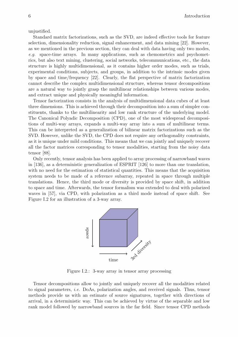
Only recently, tensor analysis has been applied to array processing of narrowband wavesin [136], as a deterministic generalization of ESPRIT [126] to more than one translation,with no need for the estimation of statistical quantities. This means that the acquisitionsystem needs to be made of a reference subarray, repeated in space through multipletranslations. Hence, the third mode or diversity is provided by space shift, in additionto space and time. Afterwards, the tensor formalism was extended to deal with polarizedwaves in [57], via CPD, with polarization as a third mode instead of space shift. SeeFigure I.2 for an illustration of a 3-way array.

space

time 3rddiversity

Figure I.2.: 3-way array in tensor array processing

Tensor decompositions allow to jointly and uniquely recover all the modalities relatedto signal parameters, i.e. DoAs, polarization angles, and received signals. Thus, tensormethods provide us with an estimate of source signatures, together with directions ofarrival, in a deterministic way. This can be achieved by virtue of the separable and lowrank model followed by narrowband sources in the far field. Since tensor CPD methods

I.5. Contribution and Outline 7

do not need any estimation of data covariance or higher order statistics, they can handleshorter data samples.

I.5. Contribution and Outline

This thesis deals with the estimation and localization of multiple sources via tensor meth-ods for array processing, using various modalities. We include several physical diversitiesinto the tensor model, in addition to space and time: space shift, polarization, gain pattersof directional sensors, and propagation speed of seismic waves. At the beginning of myPhD, I was interested in a tensor model for narrowband waves, in particular, polarizedand seismic waves. Only afterwards, I extended all our results to the study of widebandwaves using frequency diversity, further developing the corresponding tensor formulation.

The main practical difficulty of the tensor formalism is due to the requirement of mul-tilinearity, corresponding to the separability of the underlying model. While in manysituations, such as for narrowband far-field sources, the physical model is separable, thereare still as many cases in which it is not. This thesis is an example of the possibilityto use tensors even in difficult situations, such as in the case of wideband waves, thusovercoming this problem.

Contributions Throughout my PhD, my work gave rise to the following contributions,which are listed below in chronological order.

• At first, we extended tensor analysis to the seismic volume waves, using the diversityof propagation speed as a third mode. This was published in a journal article forSignal Processing, Elsevier [117].

• We also presented our work on the tensor model for narrowband polarized elas-tic waves, and its performance bounds, at a national French conference in SignalProcessing [115].

• Our interest for seismic waves lead us to publish a journal article for Signal Pro-cessing, Elsevier, on multidimensional factorization of seismic data cubes for helio-seismology [118].

• We introduced the use of directional sensors, proposing gain patterns as a physicaldiversity of its own in an article for IEEE Signal Processing Letters [116].

• After realizing that the speed diversity of seismic waves in our article [117] could beinterpreted as a frequency diversity, we decided to extend the tensor formalism togeneric wideband waves. Our idea of using spatial interpolation for linear uniformarrays was first presented at ICASSP 2016 in Shanghai [119].

• We further developed the original idea in [119] using bilinear transformations in ajournal article, published by IEEE Transactions on Signal Processing [114].

This PhD thesis is organized as follows. The presentation is divided into three parts:Part I describes the state of the art of sensor arrays and tensor analysis; Part II and Part IIIexplain my contribution for tensor array processing and multidimensional factorization,respectively.

8 Introduction

Chapter 1 presents the physical model of narrowband elastic sources in the far field,as well as the main definitions and assumptions. Chapter 2 reviews the state of the arton direction of arrival estimation, with a particular emphasis on high-resolution signalsubspace methods.

Chapter 3 introduces the tensor formalism, namely the definition of multi-way arraysof coordinates, the main operations and multilinear decompositions. Chapter 4 presentsthe subject of tensor array processing via rotational invariance.

Chapter 5 introduces a general tensor model for narrowband elastic waves, dealingwith multiple physical diversities, such as space, time, space shift, polarization, and gainpatterns .

Subsequently, Chapter 6 and Chapter 8 establish a tensor model for wideband coherentarray processing. We propose a separable coherent focusing operation through bilineartransform and through a spatial resampling, respectively, in order to ensure the multi-linearity of the interpolated data. We show via computer simulations that the proposedestimation of signal parameters considerably improves, compared to existing narrowbandtensor processing and wideband MUSIC. Throughout the chapters we also compare theperformance of tensor estimation to the Cramer-Rao bounds of the multilinear model,which we derive in its general formulation in Chapter 7. Moreover, in Chapter 9 we pro-pose a tensor model via the diversity of propagation speed for seismic waves and illustratean application to real seismic data from an Alpine glacier.

Finally, the last part of this thesis in Chapter 10 moves to the parallel subject ofmultidimensional spectral factorization of seismic ways, and illustrates an application tothe estimation of the impulse response of the Sun for helioseismology.

Part I.

Tensor Decompositions for SourceLocalization: State of the Art

1. Sensor Arrays: Parametric Modelingfor Wave Propagation

1.1. Introduction

This first chapter formulates a general model for array processing of various impingingwaves (electromagnetic or acoustic signals). A sensor array is generally an acquisitionsystem composed of multiple sensors located at different positions. This set of sensorsreceives and samples impinging sources in space and time, measuring physical quantitiessuch as electromagnetic field, pressure, particle displacement or velocity. An illustrationis given in Figure 1.1.

array

surface

source

z

yx

Figure 1.1.: Acquisition system for array processing

Array processing consists in filtering signals in a space-time field, by exploiting theirspatial characteristics, in order to estimate their parameters of interest [151]. In Sec-tion 1.2 we define and describe the narrowband model, through the introduction of thedirection of arrival as the main parameter of interest. In Section 1.3 we postulate somesimple assumptions for the acquisition configuration, and for incoming signals, such asthe far field approximation, and noise correlation structure. We state some statisticalassumptions about data collection and basic geometrical properties of the sensor arrayare reviewed. Moreover, we define the concepts of array manifold, signal subspace andnoise subspace.

In Sections 1.4 and 1.5 we extend the model in Section 1.2 to polarized, widebandand seismic waves through linear algebra tools. We parameterize polarized signals with

12 1. Sensor Arrays: Parametric Modeling for Wave Propagation

respect to both their direction of arrival and their polarization parameters. In Section 1.6we briefly describe the main properties of seismic waves.

In Section 1.7 we build a vector of parameters of interest. Finally, in Section 1.8 wederive the sample covariance matrix as an important tool carrying spatial information onimpinging sources.

1.2. Narrowband Wave Propagation for Array Processing

1.2.1. Far Field Approximation of Narrowband Waves

Many physical phenomena can be described by wave propagation through a medium, suchas electromagnetic waves through space or acoustic waves through a guide, as describedby the homogeneous wave equation

∇2E − 1

c2

∂2E

∂t2= 0 (1.1)

where c refers to the propagation speed in the medium of interest. If ‖η‖ = 1/c, anyfunction of the form f(t− pTη) is a solution to (1.1) at radius p and time t: it indicatesa wave propagating in the direction of slowness vector η with propagation speed 1/‖η‖.At first we will only consider one of the scalar components of the vector field E(p, t),whereas in Section 1.4 we will cover the model of the vector wavefield for elastic waves.

An emitting narrowband source E(0, t) = s(t)eωct can be seen as the boundary condi-tion for (1.1). The corresponding far field solution is given by

E(p, t) = s(t− pTη) eωc(t−pTη) ≈ s(t) e(ωct−p

Tκ) (1.2)

provided s(t) is a slowly varying envelope function, compared with the carrier eωct, andfor ‖p‖ c/Bs where Bs is the bandwidth of s(t). In (1.2) κ refers to the wave-vector,pointing in the direction of propagation and with modulus ‖κ‖ = ωc/c = 2π/λ, whereλ indicates the wavelength [79]. Denote by ω the radial frequency: we will restrict ourinterest to bandpass complex envelopes, that are limited in bandwidth to the region|ωL| ≤ 2πBs/2 with ωL , ω − ω0. We refer to Section 1.A for the definition of complexenvelope.

In the near field the wavefront (i.e. all the points sharing equal phase) correspondsto a sphere of radius ∆, whereas in the far field the radius is so large with respect tothe size of the array, that the field curvature becomes negligible and the wavefront canbe approximated by a plane. Therefore, spherical waves can be approximated by planewaves in the far field.

If the medium is linear, the superposition principle allows us to model multiple wavespropagating simultaneously:

x(p, t) =R∑r=1

sr(t) e(ωct−pTκr) + n(p, t) (1.3)

where n(p, t) refers to additive noise. Since (1.3) is a function of both space and time, itis particularly adequate to model signals with different space-time parameters, as we willsee in Section 1.2.2.

1.2. Narrowband Wave Propagation for Array Processing 13

1.2.2. Parametric Modeling for Sensor Arrays: Directions of Arrival

Array processing consists in merging time and space information measured at differentsensors, in order to estimate relevant signal parameters. As much as one single sensorsamples a signal in time, an array made of multiple sensors samples a wavefield in space.An antenna array is then a system exploiting two kinds of physical diversity: time andspace simultaneously. Since we can associate to each sensor in space a given time delay dueto finite propagation speed c (cf. (1.2)), we will need a time-space processing approachand make full use of our knowledge on the geometry and sensor characteristics of theacquisition system. The model in (1.3) is used in array processing for the estimationof relevant signal parameters, such as the DoA, detailed in the present section, sourcepolarization, detailed in Section 1.4, source waveforms and temporal frequency.

We consider R radiating narrowband sources in the far-field, sr, 1 ≤ r ≤ R, arrivingfrom directions defined by unit vectors d(θr), θr being a pair of angles in 3D, or a singleangle in 2D (cf. Section 1.2.3). These sources impinge on an arbitrary array of L sensorslocated at positions p` in space, 1 ≤ ` ≤ L.

We shall state the main assumptions:

A 1.1. Impinging sources are described by plane waves. This is equivalent to the far-fieldconfiguration described in Section 1.2.1. The distance of the source from the receivingarray is much greater than the array aperture: this is equivalent to assuming a planarwavefront at the sensor level. Moreover, sensors and sources are considered point-like,as their size is negligible with respect to the source-to-sensor distance (point-source andpoint-like sensors).

A 1.2. Complex envelopes have a band-limited spectrum: |ωL| ≤ 2πBs/2 with ωL , ω−ω0.

A 1.3. The narrowband assumption requires that

∆τmaxBs 1 (1.4)

where Bs is the bandwidth of source envelope s and ∆τmax is the maximum travel timebetween any two elements of the array.1 This is equivalent to requiring that the arrayaperture ∆p = ∆τmax/c (converted into wavelengths) be much less than the inverserelative source bandwidth Bs:

∆p c/Bs ⇐⇒ ∆p/λ f/Bs (1.5)

where f = ω/(2π). This allows us to represent envelope s as slowly varying: s(t−τ) ≈ s(t).

A 1.4. Narrowband in base-band. Signals of interest are the product of a varying am-plitude (complex envelope) sr(t) and a high-frequency signal eωt (cf. Section 1.2.1). Weassume that the spectral supports of both parts do not overlap (this is sometimes referredto as the Bedrosian condition)2. Under this condition, one can work in base-band withthe complex envelope of the low-pass signal. For this type of signal, a time delay of theoriginal signal is equivalent to a phase shift of the complex envelope, as expressed in (1.2).

1 For an linear array the maximum travel time refers to a source arriving along the array axis (endfire).2We recall the Bedrosian theorem [9]: The Hilbert transform of the product of two complex valued

functions f, g : R→ L2(R) with non-overlapping Fourier spectra (F (ω) ≈ 0 for |ω| > a and G(ω) ≈0 for |ω| < a where a is a positive constant) is given by the product of the low-frequency signal f andthe Hilbert transform of the high-frequency signal g: Hf(x)g(x) = f(x)Hg(x), x ∈ R.


A 1.5. Dissipation at the antenna scale is excluded, as the array dimensions are negligiblewith respect to dissipation characteristic length.

A 1.6. Sources propagate in a non-dispersive medium i.e. their propagation speed isindependent of frequency.

A 1.7. Homogeneous and isotropic medium at the antenna level : ray-paths can be ap-proximated by straight lines.

From (1.3), the signal received at the `-th sensor at time t can be modeled as:

x`(t) =R∑r=1

g`(θr) sr(t) e−ωτ`(θr) + n`(t) (1.6)

where sr(t) is the complex envelope of the r-th source, t ∈ 1, 2, . . . T, g`(θr) is the sensorgain of the `-th sensor, and n`(t) is an additive noise. It is assumed that the output in (1.6)is proportional to the wavefield (1.3) measured at its location. Notice that we droppedthe carrier term eωt, which is equivalent to converting the signal to the baseband andreducing it to its complex envelope [79].

The delay of arrival τ`(θ) is directly related to sensor locations and DoAs via theexpression

τ`(θr) = pT` κr = pT` d(θr)/c (1.7)

c being the wave propagation speed. After introducing the notion of steering element,

a`(θr) = g`(θr) e−ωτ`(θr) (1.8)

(1.6) simplifies to

x`(t) =R∑r=1

a`(θr) sr(t) + n`(t) (1.9)

The array output vector x(t) = [x1(t), . . . , xL(t)]T is then obtained by

x(t) =R∑r=1

ar sr(t) ∈ CL (1.10)

with steering vector ar = a(θr) = [a1(θr), . . . , aL(θr)]T. After arranging all the steer-

ing elements into a steering matrix and the complex envelopes into a vector of signalwaveforms

A(θ) = [a(θ1), . . . ,a(θR)] ∈ CL×R

s(t) = [s1(t), . . . , sR(t)]T ∈ CR(1.11)

(1.10) writes

x(t) = A(θ) s(t) ∈ CL (1.12)

which constitutes the general formulation for array processing. The r-th column of A(θ),denoted ar or a(θr) in the remainder, is the value of the array manifold taken at θ = θr(cf. Section 1.3).


y

z

x

O

d

source

θ

ψ

Figure 1.2.: Direction of Arrival (DoA) in 3D

1.2.3. General Array Geometries

The DoA is defined by two angles in 3D: the azimuth θ ∈ (−π, π] and the elevationψ ∈ [−π/2, π/2), as illustrated in Figure 1.2. The unit vector pointing in the direction ofthe source is then expressed by

d(θ, ψ) =

cos θ cosψsin θ cosψ

sinψ

(1.13)

On the other hand, in 2D the sources lie in the same plane as a planar array, i.e.ψ = 0, as illustrated in Figure 1.3: the DoA is then defined by azimuth θ only, leading todirectional vector

d(θ) =

[cos θsin θ

](1.14)

Hence, in a 3D space, the DoA parameter matrix Θ is an R× 2 matrix, whereas in 2Dit is a R× 1 vector (see Section 1.7 for more details).

In the remainder we will consider mostly 2D settings, as in Figure 1.3, i.e.

A 1.8. Sources and antennas are assumed coplanar, without any loss of generality. Vec-tors p` and d(θ) are thus both in R2, and we shall use the notation p` = [px` , p

y` ]

T andd(θ) = [cos θ, sin θ]T. This permits to parameterize DoAs by a single angle, azimuth θr.Therefore, unless otherwise specified, θ = [θ1, . . . , θR]T, leading to a time delay at sensor` of the form

τ`(θr) = (px` cos θr + py` sin θr)/c (1.15)

We state an important definition of the ability of a sensor array to correctly estimateany DoA:


x

y

reference sensor

`

p`

source

θ

Figure 1.3.: Acquisition system and DoA in 2D

Definition 1.1. The sensor position vectors p1, . . . ,pL are said to be resolvent withrespect to a direction v ∈ R2, if

∃k, ` : v = pk − p` s.t. 0 ≤ ‖v‖ ≤ λ/2 (1.16)

where λ refers to the wavelength of the impinging signal.

1.2.4. Uniform Linear Arrays

The most common array configuration is the Uniform Linear Array (ULA), with p` =[(`− 1)p0, 0]T, i.e. there are L elements located on the x-axis with uniform spacing equalto p0 [151], as in Figure 1.4. We have chosen the first sensor position as the origin of thecoordinate system.

1 ` L

p` x

source

dθ

Figure 1.4.: Uniform Linear Array (ULA)

In this case, if all the sensors share the same directivity pattern g(θ), the resultingsteering vector is Vandermonde:

a(θ) = g(θ)[1 e−κ0p0 cos θ, . . . , e−κ0(L−1)p0 cos θ] (1.17)


px0

py0

(a) Uniform Rectangular Array (b) Uniform Circular Array

Figure 1.5.: Regular planar array geometries

The space-time field is band-limited in wavenumber space [151]:

|κ| ≤ 2π

λ, κ0 (1.18)

with κ = κ0 cos θ = 2π cos θ/λ. This implies a spatial sampling condition upon inter-sensor spacing:

p0 ≤λ

2(1.19)

as wavenumber and position are dual FT variables. A ULA with p0 = λ2

is referred to asa standard ULA.

1.2.5. Uniform Rectangular Arrays

Analogously, for Uniform Rectangular Array (URA) as in Figure 1.5a, with px` = (`x −1)px0 , 1 ≤ `x ≤ Lx and py` = (`y − 1)py0, 1 ≤ `y ≤ Ly, we would have two conditions:

|κx| ≤ 2πλ

=⇒ px0 ≤ λ2

|κy| ≤ 2πλ

=⇒ py0 ≤ λ2

(1.20)

1.2.6. Uniform Circular Arrays

Another array configuration in 2D is the Uniform Circular Array (UCA), as in Figure1.5b, where

p` = ρ

[cos (2π(`− 1)/L)sin (2π(`− 1)/L)

](1.21)

A sampling theorem argument indicates [151]

L ≥ 2

(2πρ

λ

)+ 1 (1.22)

which ensures that the spacing between two consecutive elements is dcirc ≤ λ2.

In the remainder, we will use the following assumption on sensor spacing ∆p` = p`+1−p`:

A 1.9. Two consecutive sensors are always spaced by less than λ/2: ‖∆p`‖ ≤ λ/2, ∀`.


1.3. The Signal Subspace and the Spatial Covariance

1.3.1. Assumptions and Fundamental Definitions

We can assume the following properties, that we will use regularly throughout this thesis:

A 1.10. The number of sources, R, i.e. the model order, is known.

A 1.11. Noise spatial coherency is known. Therefore, one can always consider (thanksto spatial prewhitening) that the noise covariance matrix Σn is proportional to identity:Σn = E[n(t)n(t)H] = σ2I, where σ may be unknown, after whitening is applied. Thishypothesis refers to the spatial whiteness of noise: the noise processes at different sensorsare considered to be identically distributed and uncorrelated from one another.

A 1.12. Finally, noise is additive and Gaussian complex circular: E[n(t)n(t)T] = 0.

In Section 2.9 we address the case of spatially correlated noise.Moreover, whenever we talk about the signal subspace, we use the following assump-

tions:

A 1.13. The number of sources of interest, R, is smaller than the number of sensors L:R < L.

A 1.14. Incident signals are uncorrelated to noise.

Whenever not specified, we will assume that

A 1.15. Received sources are uncorrelated, i.e. E [sr(t)sq(t)] = 0, ∀q 6= r. Moreover,received sources sr are assumed complex Gaussian zero mean random processes withvariance σ2

r .

As for the signal covariance matrix RS = E[s(t)s(t)H], we distinguish between a fewcases:

1. If the R sources are uncorrelated, the matrix RS is diagonal and hence full rank (ornonsingular);

2. If the R sources are partially correlated, the matrix RS is nondiagonal and nonsin-gular but with worse conditioning3 than the uncorrelated case;

3. If the R sources are highly correlated, the matrix RS is nondiagonal and nearlysingular (very bad conditioned).

4. If the R sources are fully correlated or coherent, the matrix RS is nondiagonal andrank-deficient (or singular).

3 We define the condition number of a matrix A as κ(A) = ‖A‖ · ‖A−1‖. If we use the l2 norm,

κ(A) = σmax(A)σmin(A) , where σmax and σmin are the largest and the smallest singular values of matrix A.

κ(A) ∈ [1,∞): if A is unitary (AT = A−1), κ(A) = 1; if A is singular, κ(A) = ∞. If κ(A) is closeto 1, matrix A is said to be well conditioned and its inverse can be computed with good numericalaccuracy; if it is much larger than 1, A is said to be ill conditioned and its inverse will be subject tolarge numerical errors [53].

1.3. The Signal Subspace and the Spatial Covariance 19

Impinging sources are said incoherent if they are not fully correlated. In Section 2.9 weaddress the case of correlated sources.

Additional hypotheses or notations are progressively introduced when needed:

A 1.16. Identical sensor responses (calibration): all sensors have the same gain: g`(θ) =g(θ) ∀`, or they have unit gain in all directions: g`(θ) = 1 ∀`, ∀θ.A 1.17. The number of time samples T is greater than the number of sensors L: T > L.

1.3.2. Array Manifold and Signal Subspace

The R vectors ar = a(θr) ∈ CL, i.e. the columns of steering matrix A(θ), are elements ofa set (not a subspace) named array manifold or A [126], composed of all obtained steeringvectors as θ ranges over the entire parameter space4. In order to avoid ambiguities, wemake a further assumption:

A 1.18. The map from the set of DoAs θ = [θ1, . . . , θR] to RA(θ), the subspacespanned by the columns of A(θ), is injective. This can be assured by proper arraydesign.

If R < L (fewer sources than sensors, Assumption A 1.13), in the absence of noise,the array output x(t) = A(θ)s(t) =

∑Rr=1 arsr(t) is constrained into an R dimensional

subspace of CL, termed signal subspace or SX , that is spanned by the columns ar ofsteering matrix A(θ):

SX = RA(θ) =

k∑r=1

sr ar | k ∈ N,ar ∈ A, sr ∈ C

(1.23)

The noise subspace is defined as the orthogonal complement in CL of the signal sub-space, S⊥X , thanks to assumptions A 1.11, A 1.13, A 1.14 and A 1.15.

Since the signal parameters of interest are related to space, the spatial covariance isfundamental for their estimation:

RX = E[x(t)x(t)H

]=

= AE[s(t)s(t)H

]AH + E

[n(t)n(t)H

]=

= ARSAH + σ2I

(1.24)

where we used assumption A 1.11. Let us apply a spectral factorization to the arrayspatial covariance, by sorting the eigenvalues in descending order:

RX = ARSAH + σ2I = UΛUH (1.25)

where U is unitary and Λ = Diagλ1, λ2, . . . , λL, with λ1 ≥ λ2 ≥ · · · ≥ λL. Hence,(1.25) can be written as

RX = USΛSUHS +UNΛNU

HN (1.26)

with ΛS = Diagλ1, λ2, . . . , λR and ΛN = σ2I, which is equivalent to λR+1 = λR+2 =· · · = λL = σ2. Notice that US = [u1| . . . |uR] is formed by the R eigenvectorscorresponding to the first leading eigenvalues and spanning the signal subspace, andUN = [uR+1| . . . |uL] is composed of the remaining eigenvectors, spanning the noise sub-space. If matrix RX is full rank, the following facts are verified:

4For azimuth only estimation, A(θ) is a rope waving in CL; for both azimuth and elevation estimation,A(θ) is a sheet in CL.


1. the columns of US span the same space as the columns of A i.e. the column spaceof A and US coincide: RA = RUS;

2. the columns of UN span its orthogonal complement (i.e. the left null space of A)5.

Even more so, the columns of US are an orthonormal basis for the column space of A,and the columns of UN are an orthonormal basis for the left null space of A. The signalsubspace and noise subspace correspond to the column space and the left null space of Arespectively, with projectors

ΠS = USUHS = A

(AHA

)−1AH

ΠN = UNUHN = I −A

(AHA

)−1AH

(1.27)

1.4. Polarized Waves

1.4.1. The 3C Sensor Response

Sections 1.2.1 and 1.2.2 refer to a scalar wavefield, whereas the present section will derivea parametric modeling for elastic vector wavefields, or polarized waves [3]. For the moregeneral formulation of electromagnetic waves, we refer the interested reader to [96].

Let us introduce the concept of seismic vector sensor, measuring particle motion alongthree orthogonal directions. The measured physical quantity is the particle displacementrecorded by the three components of a geophone, located at a given point in space, alongthe direction of the x-, y-, and z- axes of its reference system. The z-axis is required tobe perpendicular to the earth’s surface.

Analogously to the scalar array output described in Section 1.2.2, the vector sensoroutput excited by a single source s(t) is then expressed as:

x(t) = k(ϑ) s(t) + n(t) ∈ C3 (1.28)

where k(ϑ) refers to the response vector of the sensor and is parameterized by four anglesϑ = [θ, ψ, α, β]: azimuth θ, elevation ψ, orientation angle α, and ellipticity angle β.

A narrowband polarized wave s(t) induces an elliptical particle motion x(t) that isrestricted to a plane [3]. This polarization plane is spanned by the vectors of a 3 × 2matrix H , that we choose as an orthonormal basis, as in Figure 1.6.

The restriction of the particle motion within this plane is expressed through x(t) ∈RH, or, equivalently,

x(t) = H(θ, ψ) ξ(α, β, t) + n(t) (1.29)

where ξ ∈ C2 describes the elliptical motion. Notice that ξ ∈ C2 is directly related topolarization parameters and has a unique and separable representation:

ξ = W (α)w(β) s(t) (1.30)

where matrixW performs a rotation of the ellipse principal axis of angle α ∈ (−π/2, π/2],and vector w draws the ellipse with ellipticity β ∈ [−π/4, π/4]:

W (α) =

[cosα sinα− sinα cosα

], w(β) =

[cos β sin β

](1.31)

5 The left null space of the linear map represented as the L × R matrix A is defined as the null spaceof AH: Left NullA = v ∈ CL | AHv = 0 [53].

1.4. Polarized Waves 21

y

z

x

O

dh2

h1 source

θ

ψ

Figure 1.6.: Plane of particle motion


Finally, the resulting sensor output for R impinging sources writes:

x(t) =R∑r=1

kr sr(t) + n(t) ∈ C3 (1.32)

with kr = H(θr, ψr)W (αr)w(βr) (1.33)

This model completely separates DoA, polarization parameters and time.We can distinguish between two kinds of seismic waves:

1. Transverse waves : the plane of particle motion is perpendicular to the direction ofpropagation. This means that the columns of matrix H are an orthonormal basisfor the plane perpendicular to d, as in Figure 1.7a:

HT = [h1,h2] =

− sin θ − cos θ sinψcos θ − sin θ sinψ

0 cosψ

(1.34)

Notice that d,h1,h2 forms a right orthonormal triad.

2. Tilted generalized Rayleigh waves : the polarization plane spanned by the ellipsesemi-axes contains d and h2, as in Figure 1.7b. This means that

HTGR = [d,h2] =

cos θ cosψ − cos θ sinψsin θ cosψ − sin θ sinψ

sinψ cosψ

(1.35)

Particular degenerate cases are longitudinal or P -waves, where α = β = 0 (theparticles move along the direction of propagation); and Rayleigh waves, which areelliptically polarized surface waves with ψ = α = 0. See Section 1.6 for more detailsabout seismic waves and polarization.

1.4.2. Vector Sensor Arrays

The present section combines results from Sections 1.4.1 and 1.2.2, deriving the parametricmodel for an array composed of L vector, i.e. three-component sensors (3Cs) [3], as inFigure 1.8.

The array output at time t is given by an L× 3 matrix

X(t) = [yT1 , . . . ,y

TL] (1.36)

If all previous assumptions are verified, combining (1.10) and (1.32) yields

X(t) =R∑r=1

ar ⊗ kr sr(t) +N (t) =

= AS(t)KT +N (t)

(1.37)

with steering vector ar = a(θr, ψr), and polarization vector kr = k(θr, ψr, αr, βr). More-over, S(t) = Diags1(t), . . . , sR(t), K = [k1, . . . ,kR] refers to the 3×R sensor responsematrix, and A = [a1, . . . ,aR] refers to the L×R array steering matrix.

1.4. Polarized Waves 23

h1

h2

h1h2

cos(β)

sin(β)

α

(a) Polarization ellipse - TR waves

d

h2

dh2

cos(β)

sin(β)

α

(b) Polarization ellipse - TGR waves

Figure 1.7.: Orientation and ellipticity of the polarization ellipse

Figure 1.8.: 3C sensor


We can vectorize the array output matrix at time t as the C3L vector x(t) = vecX:

x(t) =R∑r=1

kr ar sr(t) + n(t) =

= K A s(t) + n(t)

(1.38)

where s(t) = vecS(t) and n(t) = vecN (t). Notice that the polarized signal subspaceis spanned by column vectors k1 a1, . . . ,kR aR.

1.4.3. Another Polarization Model

In many polarimetric applications, such as RADAR, the vector sensor has P components:we can model the signal received at component p by multiplying its amplitude by ρp andshifting its phase by φp, relative to the first (reference) component p = 1 [92, 44]:

k(ρ,φ) =[1, ρ1e

φ1 , . . . , ρP eφP]T

(1.39)

where ρ = [1, ρ1, . . . , ρP ]T, and φ = [1, φ1, . . . , φP ]T. Thus polarimetric models in (1.37)and (1.38) attain a decoupled form

X(t) =∑R

r=1 ar ⊗ kr sr(t) +N (t) ∈ CL×P

x(t) =∑R

r=1 kr ar sr(t) + n(t) ∈ CLP(1.40)

in which steering vector ar = a(θr, ψr), and polarization vector kr = k(ρr,φr) dependon distinct parameters. DoA and polarization information are then decoupled.

1.5. Wideband Sources

1.5.1. Wideband Scalar Wavefields

Let us consider a wideband wavefield with carrier ωc: E(p, t) = s(t− pTκ)eωct measuredat position p and time t, and its Fourier Transform (FT)

E(p, ω) =

ˆ ∞−∞

E(p, t)e−ωtdt (1.41)

If the spectral bandwidth Bs of the complex envelope s(·) is not negligible in (1.5), atime delay is not equivalent to a phase shift anymore: s(t − τ) 6= s(t)e−ωτ . However,thanks to the time shift theorem of FT F(·), a translation in time domain translates intoa phase shift in frequency domain:

s(t− τ)←→ s(ω)e−ωτ (1.42)

where s = F(s). Therefore, in order to use the spatial information of the acquisitionsystem, we need to work with Fourier transformed data.

The real wideband signal received at the `th sensor at time t can be modeled as

x`(t) =R∑r=1

g`(θr)sr(t− τ`(θr)) + n`(t), (1.43)

where sr(t) is the signal transmitted by the rth source, t ∈ 1, 2, . . . T, g`(θr) is the gainof the `th sensor, τ`(θr) was defined in (1.7) and n`(t) is an additive noise. We make onefurther assumption:

1.5. Wideband Sources 25

A 1.19. Sensor gains g` are a priori unknown functions unless otherwise specified, real(which is actually equivalent to assuming that their phase is known) and independent offrequency.

Denote by x(ω) the FT of x(t). In this framework, thanks to (1.42), model (1.43) canbe equivalently rewritten in the frequency domain:

x`(ω) =R∑r=1

a`(ω, θr)sr(ω) + n`(ω) (1.44)

where x`(ω) = Fx`(t) is the FT of x`(t), and ω = ω1, . . . , ωQ if we take the DiscreteFourier Transform (DFT); n`(ω) refers to a circular Gaussian white noise process at the`-th sensor, thanks to Assumption 1.12. Notice that the steering element

a`(ω, θr) = g`(θr) e−ωτ`(θr) (1.45)

is now a function of both frequency and DoA.Alternatively, in vector form, (1.44) becomes

x(ω) =R∑r=1

a(ω, θr) sr(ω) + n(ω) =

= A(ω,θ) s(ω) + n(ω)

(1.46)

where matrix A(ω,θ) ∈ CL×R depends on the vector of DoAs, θ = [θ1, .., θR]T. Thanksto Assumption 1.11, noise n(ω) is circular complex white Gaussian, with covariance σ2I.The r-th column of A(ω,θ), denoted ar(ω) = a(ω, θr) in the remainder, is the value ofthe array manifold for radial frequency ω taken at θ = θr. Therefore, the array manifoldand the signal subspace are now frequency dependent. Moreover, notice that also spatialcovariance RX in (1.24) becomes frequency dependent:

RX(ω) = E[x(ω)x(ω)H

](1.47)

1.5.2. Polarized wideband sources

This section combines the wideband scalar model in Section 1.5.1 with wave polarizationin Section 1.4. For this purpose, we will need a further assumption:

A 1.20. The polarization parameters α and β of impinging wavefronts are independentof frequency.

Wideband output in (1.38) and polarized output (1.46) combined together yield a L×3wideband polarized output:

X(ω) =R∑r=1

ar(ω)⊗ kr sr(ω) +N (ω) =

= A(ω)S(ω)KT +N (ω)

(1.48)

with steering vector ar(ω) = a(ω, θr, ψr), and polarization vector kr = k(θr, ψr, αr, βr).Moreover, S(ω) = Diags1(ω), . . . , sR(ω), K = [k1, . . . ,kR] refers to the 3 × R sensorresponse matrix, and A(ω) = [a1(ω), . . . ,aR(ω)] refers to the L×R array steering matrix.


We can vectorize the array output matrix at frequency ω as the C3L vector x(ω) =vecX(ω)

x(ω) =R∑r=1

kr ar(ω) sr(ω) + n(ω) =

= K A(ω) s(ω) + n(ω)

(1.49)

where s(ω) = vecS(ω) and n(ω) = vecN (ω). Notice that the polarized signalsubspace at frequency ω is spanned by column vectors k1 a1(ω), . . . ,kR aR(ω).

1.6. Seismic Waves

The importance of sensor arrays for the analysis of seismic waves was illustrated in [123].As we briefly mentioned in Section 1.4, [3] made a simple inventory of seismic wavesaccording to their polarization type. More generally, we can distinguish between volumeor body waves and surface waves [133, 134] .

Volume or body waves

Two types of waves can propagate through a homogeneous isotropic solid medium, onecorresponding to changes in dilatation and the other to rotation [134].

Direction of propagation

Particle motion

(a) Particle motion of P waves

Direction of propagation

Particle motion

(b) Particle motion of S waves

Figure 1.9.: Particle motion of seismic volume waves

• P waves (or primary, dilatational, compressional, irrotational, longitudinal waves).Since their particle motion is parallel to the direction of propagation, as in Figure1.9a, they are linearly polarized.

1.6. Seismic Waves 27

• S, SH, SV waves (or transverse, shear, rotational, secondary): their particle motionlies in the plane perpendicular to the direction of propagation, as in Figure 1.9b.They can be linearly or elliptically polarized.

Linear polarization refers to the fact that more coherent seismic energy is located in oneprincipal direction of particle motion [98].

Seismic events originating at depth, one has to deal with a double arrival of elasticbody waves: P waves and S waves. They have different propagation velocities and avariable frequency content: the former tend to have a higher frequency content and arecharacterized by higher propagation speed than the latter. Hence, the P wave arrivesfirst, whereas the S wave is the second arrival observed on seismic records. P waves andS waves have theoretical velocities v1 and v2, respectively, given by Ref. [133]:v1 =

(λ+2µρ

) 12

v2 =(µρ

) 12

(1.50)

where λ and µ are Lame’s constants and ρ is the density of the medium. Since they arepositive constants, v1 is greater than v2. In particular, the velocity of the S wave rangesfrom zero up to 70% of the velocity of the P wave. For fluids µ is zero, v2 = 0 andtherefore S waves do not propagate. Typical velocities are in the 1.5km/s (in water) to6.5km/s range, increasing with loss of porosity, cementation, age and depth [134].

For the physical model of wave propagation, the following property is assumed:

A 1.21. P and S waves propagate at velocities v1 and v2, respectively, under the approx-imation of non-dispersive medium A 1.6.

Surface waves

When the xy-plane separates two media with different properties, solutions decreasinglike e−κz (evanescent waves) exist under certain conditions. Their amplitude decreasesexponentially with the distance from the interface, and their energy is tied to the surface[134].

• Rayleigh waves, surface elliptically polarized waves with the ellipse major axis cor-responding to the direction of propagation. They propagate along a free surface ofa solid, where free means contact with vacuum or with air, as the elastic constantand density of air are negligible compared with that of rocks. Rayleigh waves areoften referred to as ground roll. They are dispersive, low velocity, low frequency,with a broad flat spectrum [133].

• Other examples include Stoneley waves, Love waves, Tube waves.


1.7. Parameters of Interest

In the first part of this chapter we described the model of plane waves with unknownwavenumber impinging into the array. The parameters of interest ϑ enter into the model ina non linear way. The problem of estimating the source wavenumbers or angles of arrivalsof multiple plane waves is referred to as Direction of Arrival or DoA estimation. Thisproblem is widespread in many scientific domains, such as radar, sonar, seismic, medicaldiagnosis and astronomy [151]. The narrowband model we refer to in the remainder isdeveloped in Section 1.2.2, whereas the wideband model can be found in Section 1.5.1.

As we explained in Section 1.2.3, in 3D for a single plane wave, the parameters ofinterest form a vector: ϑ = [θ, ψ]T ∈ R2; in 2D it is a scalar ϑ = θ ∈ R. With R sources,this corresponds to

Θ = [θ,ψ] =

θ1 ψ1...

...θR ψR

∈ RR×2, θ =

θ1...θR

∈ RR (1.51)

respectively. In the case of polarized waves, we might also be interested in estimating thepolarization parameters φ = [α, β]T ∈ R2, or, for R sources:

Ξ = [α,β] =

α1 β1...

...αR βR

∈ RR×2 (1.52)

We can arrange all parameters of interest into a vector ϑ:

1. For scalar wavefields in 3D, we have:

ϑ = [θT,ψT]T =

= [θ1, . . . , θR, ψ1, . . . , ψR]T ∈ R2R(1.53)

2. For scalar wavefields in 2D, we have:

ϑ = θ = [θ1, . . . , θR]T ∈ R (1.54)

3. For vector wavefields in 3D, we have:

ϑ = [θT,ψT,αT,βT]T =

= [θ1, . . . , θR, ψ1, . . . , ψR, α1, . . . , αR, β1, , . . . , βR]T ∈ R4R(1.55)

4. For vector wavefields in 2D, we have:

ϑ = [θT,αT,βT]T =

= [θ1, . . . , θR, α1, . . . , αR, β1, , . . . , βR]T ∈ R3R(1.56)

In many cases, we might also be interested in extracting the source signaturess1(t), . . . , sR(t), which can be stored in a T ×R matrix

S =

s1(1) . . . sR(1)...

. . ....

s1(T ) . . . sR(T )

= [s1, . . . , sR] (1.57)

or a vector ξ = [sT1 , . . . , sTR]T ∈ CTR.

Other problems, which are beyond the scope of this thesis, include the following:

1.8. The Sample Covariance Matrix 29

1. Array calibration, i.e. the estimation of the positions and gains of sensors:sensor position matrix P = [p1, . . . ,pL]T ∈ RL×3;sensor gain patterns [g1(θ), . . . , gL(θ)].

2. ARMA modeling and parameter estimation.

3. Estimation of the range of near field sources.

The next chapter will introduce high resolution DoA and polarization estimation forboth narrowband and wideband impinging wavefields. We will restrain our interest to thesignal subspace approach (cf. Section 1.3 for the definition of signal and noise subspace).

1.8. The Sample Covariance Matrix

In Section 1.2.2 we derived the spatial covariance matrix in (1.24), assuming we disposeof an infinite observation period. However, the natural estimate of this quantity is thesample covariance matrix. To this purpose, we can use either the narrowband snapshotmodel in time domain or in frequency domain. In time domain we have:

RX =1

T

T∑t=1

x(t)x(t)H = XXH (1.58)

where appears the L× T data matrix X = [x(1), . . . ,x(T )].If there are multiple independent and identically distributed complex Gaussian snap-

shots available, X1, . . . ,XNS , we define the sample covariance matrix as [151]

RX =1

NS

NS∑j=1

XjXHj (1.59)

On the other hand, after DFT with Q frequency bins, frequency dependent spatialcovariance in (1.47) is estimated as:

RX(ωq) =1

NS

NS∑j=1

xj(ωq)xj(ωq)H (1.60)

If we do not impose our knowledge of the array manifold upon it, RX is the MaximumLikelihood Estimator (MLE) of the spectral matrix, and its spectral representation is

RX = USΛSUH

S + UNΛNUH

N (1.61)

The sampling process generates a sequence of Gaussian random vectors (cf. Assump-tions A 1.12 and A 1.15), we assume that resulting vectors at different time instants t,in different frequency bins ωq and different observation snapshots are statistically inde-pendent [151]. Therefore, one can prove that the time domain model and the frequencydomain model, for the narrowband case, have identical spatial statistics, resulting inidentical subsequent processing [151]. This means that if the sources are narrowband, thetwo equations in (1.58) and (1.60) have the same spatial structure, allowing us to workindifferently in time or frequency domain.

Appendix

1.A. Signal Complex Envelope

A time series x(t) can be considered a pass-band signal if its spectral support is limitedand it does not include the origin:

[−f0 −W,−f0 +W ] ∪ [f0 −W, f0 +W ], with ∞ > f0 > W > 0 (1.62)

Every pass-band signal can be associated with an analytic signal x(t) whose support doesnot contain positive frequencies:

X(f) =√

2 U+(f)X(f)←→ x(t) =1√2

[x(t) + Hx(t)] (1.63)

where U+(·) indicates the Heaviside step function, and Hx(t) refers to the Hilberttransform of real signal x(t). Since a real signal is characterized by even spectral symmetry,it can be represented by its analytic signal without loss of information.

The complex envelope of x(t) around frequency f0, or base-band signal, is obtained fromthe analytic signal by a mere translation in frequency:

X(f) = X(f + f0)←→ x(t) = x(t)e−2πf0t (1.64)

For a given carrier at frequency f0, a complex envelope around f0 is in bijection with acomplex number representing the modulus and the phase of the carrier.

2. Signal Parameter Estimation in 2D

2.1. Introduction

After introducing in Chapter 1 the basics of the sensor array model, we dedicate thepresent chapter to the problem of high resolution signal parameter estimation. In par-ticular, the parameters of interest are represented by directions of arrival, polarizationfeatures and source signatures. The term 2D in the title refers to traditional matrix ap-proaches, relying on time and space information: in the time model of (1.12) data canbe described by a matrix X ∈ CL×T for the narrowband case, and a matrix X ∈ CL×Q

for the wideband case. Useful information is derived by sampling impinging wavefields intime and space, and through the computation of the spatial covariance matrix in (1.58)and (1.60). Whenever other physical dimensions are present, such as polarization, dataare vectorized as in (1.38) and (1.49), so that their inner structure is lost and the mainrepresentation remains a long matrix X ∈ C3L×T in time domain, and X ∈ C3L×Q infrequency domain.

In Section 2.2 we lay the basis for the evaluation of the performance of an estima-tor, through the definition of the log-likelihood and the performance bound (Cramer-RaoBound). In Section 2.3 we introduce the two main approaches for signal parameter esti-mation: spectral and parametric methods.

After briefly introducing beamforming in Section 2.4, we detail the main high resolutionsignal subspace methods, MUSIC and ESPRIT, in Sections 2.5 and 2.6, respectively.These algorithms are evaluated and compared with the performance bound of Section 2.2and in terms of computational cost. Sections 2.7 and 2.8 extend the signal subspace tothe separation of polarized and wideband waves.

Finally, in Section 2.9 we discuss the case of correlated noise and correlated sources,i.e. when Assumptions A 1.11 and A 1.15 are not verified.

2.2. Performance of an Estimator

The NS snapshots xj(t) or xj(ω) introduced in Section 1.8 are statistically independent,so we can deal with one single snapshot and combine the results at the end.

As previously stated, thanks to Assumptions A 1.12, the observation x(t) or x(ω) is acomplex Gaussian random vector x whose mean µ(ϑ) and covariance RX(ϑ) depend onreal parameter vector ϑ. In the remainder, in the light of Section 1.7, ϑ is an arbitraryvector of parameters, and it does not necessarily indicate an angle [151].

The variance of any unbiased estimator is bounded by the Cramer-Rao Bound (CRB):if ϑ is modeled as deterministic, the performance of the estimator is bounded by theclassical CRB; if it is modeled as a random variable, we need a Bayesian CRB, and if itis partially random, we need a hybrid CRB. In the remainder we will assume that ϑ isfully deterministic.

32 2. Signal Parameter Estimation in 2D

The likelihood, i.e. the probability density for a single snapshot is then given by

p(x|ϑ) =1

detπRX(ϑ) exp−(xH − µH(ϑ)

)R−1X (ϑ) (x− µ(ϑ))

(2.1)

where x ∈ CL is a complex Gaussian random variable and ϑ ∈ RD is the real deterministicvector we want to estimate. In Chapter 7 we will develop the subject of the estimationof a complex parameter vector.

For i.i.d. snapshots, the likelihood is the product

p(x1, . . . ,xNS |ϑ) =

NS∏j=1

1

detπRX(ϑ) exp−(xHj − µH(ϑ)

)R−1X (ϑ) (xj − µ(ϑ))

(2.2)

The log-likelihood corresponding to (2.2) is given by

Lx(ϑ) = L(x1, . . . ,xNS |ϑ) = log[p(x1, . . . ,xNS |ϑ)] =

= −NS log [det RX(ϑ)]−NS∑j=1

(xHj − µH(ϑ)

)R−1X (ϑ) (xj − µ(ϑ))−NSL log π

(2.3)

In many cases of interest, either µ(ϑ) orRX(ϑ) (but not both) are a function of parametervector ϑ.

We denote the covariance matrix of an unbiased estimator as

C(ϑ) = E[(ϑ− ϑ)(ϑ− ϑ)T

](2.4)

The multiple parameter CRB states that [151]

C(ϑ) ≥ CCRB(ϑ) , F−1 (2.5)

for any unbiased estimate of ϑ. The matrix inequality means that C(ϑ)−CCRB is a nonnegative definite matrix. F denotes the Fisher Information Matrix (FIM):

F , −E[∇ϑ(∇ϑ(Lx(ϑ))T

)](2.6)

with elements

Fij , −E[∂Lx(ϑ)

∂ϑi

∂Lx(ϑ)

∂ϑj

]= −E

[∂2Lx(ϑ)

∂ϑiϑj

](2.7)

The result (2.5) also provides a bound on the variance of any unbiased estimate of scalarelement ϑi:

Var(ϑi − ϑi) ≥ [CCRB(ϑ)]ii = [F−1]ii (2.8)

The effect of considering multiple snapshots with respect to the single snapshot case isthat the CRB is divided by NS.

When we generate multiple realizations of the same process, we estimate the varianceVar(ϑi − ϑi) through N Monte Carlo (MC) trials, by computing the Mean Square Error(MSE):

MSE(ϑi) =1

N

N∑n=1

(ϑn − ϑi)2 (2.9)

2.3. Spectral and Parametric Approaches 33

In order to assess the performance of the unbiased estimator, we are also interested inplotting its MSE as a function of the Signal to Noise Ratio (SNR) in dB:

SNR = 10 log10

PsPn

(2.10)

where Ps and Pn refer to average signal and noise power. We are interested in comparingMSE(ϑi) with the SNR. An estimator is said efficient if it reaches the CRB, i.e. whenits variance equals the CRB: C(ϑ) = CCRB(ϑ). The Maximum Likelihood Estimator(MLE), which maximizes the log-likelihood, is asymptotically (for NS → ∞) efficient.Many other estimators come close to the CRB for high SNR: the value of the SNR atwhich this convergence occurs is referred to as threshold. Estimators with a lower thresholdSNR are said to have a better threshold behavior.

2.3. Spectral and Parametric Approaches

Before introducing the estimation of signal parameters of interest, we need to make afurther assumption:

A 2.1. In what follows, the number of impinging sources R is supposed to be known.

In Chapter 1 we modeled the array output as a function of signal parameters such asthe Directions of Arrival (DoAs) θr, ψr and wave polarization angles αr, βr. The goal ofarray processing is to estimate these parameters, starting from the the array output x(t).

We can distinguish between two main approaches [79]:

1. The spectral approach maximizes a spectrum-like scalar function of the parame-ters of interest, looking for its R highest peaks. We can include into this classbeamforming and the most known signal subspace method, spectral MUSIC.

2. The parametric approach requires a simultaneous search for all parameters, pro-viding more accurate but also more computationally expensive solutions. We caninclude into this class both deterministic and stochastic MLEs, sub-space approxi-mations, root-MUSIC and ESPRIT.

Subspace methods such as MUSIC, root-MUSIC and ESPRIT achieve higher resolutionthan conventional beamforming techniques and are thus called high resolution methods.We will briefly introduce beamforming, but we will detail in particular MUSIC and ES-PRIT, as they are among the most versatile and widespread high resolution methodsfor signal parameter estimation, though not implying the heavy computational burdenof MLE [79, 17]. Notice that MUSIC, ESPRIT and the deterministic ML belong to thegeneral class of subspace-fitting algorithms [153, 142] .

2.4. Beamforming

Beamforming (BF) builds a specific spatial response of the array (i.e. a beam pointing tothe desired source, and hopefully nulls towards other interferences) in order to estimatethe signature of the sources impinging on the array in the presence of noise. The steeringdirections that result in maximum output power are the DoA estimates. An exhaustive


search involves the presteering of the array in a given look direction θ ∈ (−π, π], byapplying a sensor dependent time delay T`(θ) = T0 + τ`(θ):

xps` (t, θ) = x`(t+ T`(θ)) ` = 0, ..., L− 1 (2.11)

where T0 is a bulk delay such that T`(θ) > 0, ∀` [51]. The BF output is then givenby y(t, θ) =

∑L`=1 x

ps` (t, θ). A time interpolation is then necessary for a correct imple-

mentation of presteering delays in order to extrapolate signal values at given time delaysbetween two original samples. The effect of presteering in a source direction θ = θr is aspatial alignment of all the waveforms on all sensors, corresponding to a local maximumenergy output when θ = θr: x

ps` (t, θr) ≈ sr(t+ T0), ∀`.

The steering operation of narrowband BF can be achieved through a linear combinationof spatial samples through weight vector w ∈ CL, in the same manner that a FiniteImpulse Response (FIR) filter linearly combine temporally sampled data [152]:

y(t) =L∑l=1

w∗` x`(t) = wHx(t) (2.12)

with associated output power

P (w) =1

T

T∑t=1

|y(t)|2 =1

T

T∑t=1

wHx(t)x(t)Hw = wH RX w (2.13)

where we observe the sample covariance matrix RX . The spatial resolution dependson the size in wavelengths of the array aperture. However, when the signal bandwidthincreases, its performance degrades. One of the first Tapped Delay Line (TDL) timedomain solutions was provided for this purpose by [47] and involves a TDL scheme (orFIR filters for the discrete case). A temporal filter is applied to each wideband recordedsignal to compensate for the phase difference of different frequency components; this isequivalent to a temporal and spatial sampling of the propagating wavefield: [89, 52]

y(k) =L∑l=1

J−1∑i=0

w∗lix`(k − iTs) = wHx(k) (2.14)

where J is the length of the filter corresponding to the TDL, Ts is the delay betweenadjacent lags of the TDL. We also need to properly define long vectors w,x ∈ CLJ . Forthe sake of simplicity, we will assume Ts equal to sampling period. Analogously to thefrequency response of a FIR filter1, when the signal is a complex plane wave with DoA θand frequency ω, we have:

y(k) = eωkL∑l=1

J−1∑i=0

w∗lieω(τ`(θ)+i) = eωkγ(ω, θ) (2.15)

where the beamformer response γ is a function of steering vector a(ω, θ):

γ(ω, θ) = wHa(ω, θ) (2.16)

1The analogy of BF and FIR filtering is closest when the sensor array is a ULA and we fix a singletemporal frequency ω0, if we establish a mapping between temporal frequency for the FIR filter andthe cosine of the DoA for the beamformer: ω = ω0p0 cos(θ)/c.

2.5. Spectral MUSIC 35

The beampattern is given by its square modulus |γ(ω, θ)|2.The type of beamformer will depend on the procedure for choosing weight vectorw: the

most common examples are Bartlett and Capon beamformers, and Linearly ConstrainedMinimum Variance (LCMV) beamformer [152]. When the number of sources increases,the performance of time domain beamforming rapidly degrades and is by far exceeded byhigh resolution techniques.

2.5. Spectral MUSIC

The interest in the subspace approach is mainly due to the introduction of the MultipleSignal Characterization (MUSIC) algorithm and its performance capability [131]: receiveddata are used to estimate the signal subspace described in Section 1.3, and then thisinformation is used to estimate signal parameters such as the DoA [79, 151]. MUSICparameter estimation relies on a fundamental assumption on the acquisition system:

A 2.2. The array manifold A = a(θ) is assumed to be known.

In the absence of noise, the steering vectors are the intersections between the signalsubspace SX and the array manifold A (see Section 1.3 for their definitions). However, inthe presence of noise, with probability one there are no intersections: SX ∩ A = ∅. Theidea behind MUSIC is to look for elements in A that are closest to SX .

As many spectral methods, MUSIC relies on the spectral decomposition of the covari-ance matrix in (1.26):

RX = USΛSUHS +UNΛNU

HN (2.17)

As previously mentioned in Section 1.3, the noise eigenvectors UN are orthogonal to thearray manifold A = a(θ1), . . . ,a(θR):

a(θr)HUN = 0, r = 1, . . . , R (2.18)

The projector and orthogonal projector of the signal subspace in (1.27) is derived fromthe noise eigenvectors of the estimated covariance matrix R:

ΠS = USUH

S

ΠN = UNUH

N = 1− USUH

S

(2.19)

We can then define the normalized MUSIC spatial spectrum:

PMU(θ) =a(θ)Ha(θ)

a(θ)HΠNa(θ)=

a(θ)Ha(θ)

a(θ)H(I − ΠS)a(θ)(2.20)

to be maximized. In the presence of noise UN 6= UN and the denominator is not zero,but its value decreases significantly. Therefore, as suggested by (2.18), the spectrum in(2.20) has peaks in correspondence of the true DoAs θr. Alternatively, one can minimize

PMU(θ) = a(θ)HΠNa(θ) = a(θ)H(1− ΠS)a(θ) (2.21)

The steps of the algorithm are the described in Algorithm 2.1.Notice that MUSIC is a two-steps sub-optimal algorithm, involving an unconstrained

estimation of a set of R vectors ur and then the maximization of a 1D function PMU(θ).


Algorithm 2.1 Spectral MUSIC

1: Compute either US or UN :

1. either through an Eigenvalue Decomposition (EVD) on sample covariance ma-trix RX ;

2. or through an Singular Value Decomposition (SVD) on raw data matrix X(recommended for computational reasons).

2: Plot the MUSIC spectrum PMU(θ, ψ) and chose the R maxima. For 2D systems, inparticular, the azimuth is given by

θr = arg maxθ∈(−π,π]

PMU(θ) (2.22)

another version of MUSIC, named root-MUSIC was proposed by [5] for ULAs, whichexhibits a threshold for lower SNR than spectral MUSIC, but with the same asymptoticproperties. DoAs are given by the R roots of a polynomial PMU,z(z) = az(1/z)TΠNaz(z),that are inside the unit circle and closest to the unit circle, with az(z) = [1 z . . . zL−1]T

andPMU,z(z)|z=e−ωp0 cos θ/c = PMU(θ) (2.23)

In the absence of noise, these roots would be exactly on the unit circle. Root-MUSIC canbenefit from the spatial backward-forward smoothing techniques described in Section 2.9.The Unitary root-MUSIC algorithm implements backward-forward root-MUSIC througha unitary transformation [108].

2.5.1. Evaluation of spectral MUSIC

The performance of MUSIC in comparison to the CRB can be found in [151, 140, 141].

Main advantages

• Arbitrary array configurations.

• Multiple parameter estimation (azimuth, elevation, range, polarization, etc.): it ispossible to estimate F parameter per source, i.e. RF signal parameters.

• Since its search assumes that one single source is present, MUSIC only looks forF parameters, instead of RF . Hence, it is less computationally expensive than theML methods.

• High resolution compared to beamforming.

• Asymptotically unbiased and efficient, if the noise is white Gaussian. For uncorre-lated signal and high SNR, spectral MUSIC is close to the CRB.

Drawbacks

• Complete knowledge of the array manifold (sensor positions and gains) is required,i.e. array calibration is necessary.

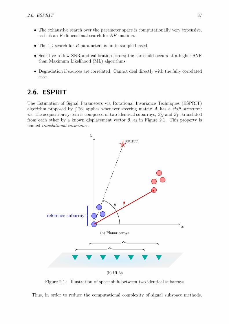
2.6. ESPRIT 37

• The exhaustive search over the parameter space is computationally very expensive,as it is an F -dimensional search for RF maxima.

• The 1D search for R parameters is finite-sample biased.

• Sensitive to low SNR and calibration errors; the threshold occurs at a higher SNRthan Maximum Likelihood (ML) algorithms.

• Degradation if sources are correlated. Cannot deal directly with the fully correlatedcase.

2.6. ESPRIT

The Estimation of Signal Parameters via Rotational Invariance Techniques (ESPRIT)algorithm proposed by [126] applies whenever steering matrix A has a shift structure:i.e. the acquisition system is composed of two identical subarrays, ZX and ZY , translatedfrom each other by a known displacement vector δ, as in Figure 2.1. This property isnamed translational invariance.

x

y

reference subarray

δ

source

θ

(a) Planar arrays

(b) ULAs

Figure 2.1.: Illustration of space shift between two identical subarrays

Thus, in order to reduce the computational complexity of signal subspace methods,


ESPRIT introduces a space shift constraint into the acquisition system in (1.9):x`(t) =

∑Rr=1 a`(θr) sr(t) + nx`(t)

y`(t) =∑R

r=1 a`(θr) e−ωδTdr/c sr(t) + ny`(t)

(2.24)

where a`(θr) = g`(θr) e−ωτ`(θr). In [126] the translation δ is assumed to be collinear

with the x-axis: δ = [δ, 0, 0], leading to e−ωδTdr/c = e−ωδ cos θr/c, without restricting the

generality. We also assume the problem is in 2D, with sources coplanar to the acquisitionplane. The array output in vector form in (1.12) becomes

x(t) = As(t) = AX s(t) ∈ CL

y(t) = AΦ s(t) = AY s(t) ∈ CL(2.25)

where x(t) and y(t) correspond to measurements recorded on the first and second subar-rays respectively, and shift invariance

AY = AXΦ (2.26)

Diagonal R × R matrix Φ is a unitary operator that relates the measurements fromsubarray ZX to those from subarray ZY :

Φ = Diage$1 , . . . , e$R (2.27)

with phase shifts $r = −ωδ cos θr/c. Notice that in the complex field Φ is a simplescaling operator, but it is isomorphic to the real 2D rotation operator (thus giving originto the name ESPRIT). The general idea is to exploit the rotational invariance of the signalsubspace introduced by the translational invariance of the sensor array, by estimating thediagonal elements of Φ, without having to know A.

Then we have the acquisition system output:

z(t) =

[x(t)y(t)

]= As(t) + nz(t) ∈ C2L (2.28)

where A =

[AAΦ

]∈ C2L×R and nz(t) =

[nx(t)ny(t)

], and covariance matrix from (1.25)

and (1.26):

RZ = ARSAH

+ σ2I =

= USΛSUHS +UNΛNU

HN

(2.29)

As discussed in Section 1.3, RUS = RA: there must exist a unique nonsingulartransformation T such that

US = A T (2.30)

Through the invariance structure of the array we can decompose US ∈ C2L×R intoUX ,UY ∈ CL×R

US =

[UX

UY

]=

[ATAΦT

](2.31)

from which we infer RUX = RUY = RA. From (2.31) we derive

UY = UX Ψ (2.32)

2.6. ESPRIT 39

with

Ψ = T−1 ΦT (2.33)

Notice that (2.32) is the equivalent relationship to shift invariance AY = AXΦ in (2.26)in terms of signal subspace eigenvectors, and that the eigenvalues of Ψ correspond to thediagonal elements of Φ. Since R < L, this is an overdetermined set of equations. Inpractice, since we have estimates for these signal subspaces, (2.32) becomes:

UX Ψ = UY (2.34)

Linear system (2.34) can be solved through a Least Squares (LS), if the whole error isattributed to UY , with solution

ΨLS = U†XUY (2.35)

or a Total Least Squares (TLS) approach, if both UX and UY are considered noisy:

(UX +EX) Ψ = (UY +EY ) (2.36)

whereEX andEY must have minimum Frobenius norm. Linear system (2.36) has solution

ΨTLS = −V 12V−122 (2.37)

where V 12 and V 22 are R×R matrices defined by the eigendecomposition of the 2R×2Rmatrix [

UH

X

UH

Y

] [UX UY

]=

[V 11 V 12

V 21 V 22

]ΛV

[V

H

11 VH

21

VH

12 VH

22

](2.38)

The steps of the algorithm are the described in Algorithm 2.2.

Algorithm 2.2 LS and TLS ESPRIT

1: Compute US:

1. either through an EVD on sample covariance matrix RZ

2. or through an SVD on raw data matrix Z (recommended for computationalreasons).

2: Select UX and UY by decomposing US from (2.31).3: Obtain ΨLS from (2.35) or ΨTLS from (2.37).4: Find the eigenvalues of ΨLS or ΨTLS: λ1, . . . , λR.5: Find the arguments of the steering complex exponentials from (2.27) as $r =

argλr, r = 1, 2, . . . , R.

LS and TLS ESPRIT have the same asymptotic behavior (for Ns → ∞), but TLSESPRIT has better threshold behavior, with a slight increase in computational complexity.We inform the interested reader that another effective formulation of this approach is givenby Unitary ESPRIT [59], that we do not discuss further.


2.6.1. Signal Copy

Estimation of signals as a function of time from a previously estimated DoA is termedsignal copy [126]. Sometimes we are not only interested in the signal parameters, but alsoin signal signatures themselves.

Although the steering matrix A is not supposed to be known, we can exploit therelationship US = A T to find it:

A = US T−1 (2.39)

where T−1 is derived from (2.33) as the eigenvector matrix of Ψ.Once we have estimated the steering matrix from (2.39), the simplest solution for the

signal copy problem consists in a linear estimator with a squared cost function in themetric of the noise Σn.2 This is equivalent to an oblique projection of the data matrix Xon the column space of A, RA:

S = W HZ (2.40)

withW = Σ−1

n A[AHΣ−1n A]−1 =

= Σ−1n US[UH

SΣ−1n US]−1T−H

(2.41)

Notice that the r-th column ofW , wr, is a weight vector that enhances the signal from ther-th DoA and reject those from other directions. This is equivalent to a spatial matchedfilter.

Since we only have an estimate of the steering matrix A, at low SNR we may resort toa more robust TLS approach (see [126] for details).

2.6.2. Evaluation of ESPRIT

The performance of ESPRIT in comparison with the CRB can be found in [151, 103].

Main advantages

• High resolution compared to beamforming, and comparable to that of MUSIC.

• Knowledge of the array manifold (sensor positions and gains) is not required: onlytranslation δ needs to be known.

• The structure of the subarray is arbitrary.

• Computationally efficient, much less expensive than the ML methods and thanMUSIC (no need for an exhaustive search).

• Computational advantage especially pronounced for high dimensional parameterestimation: ESPRIT computational load grows linearly, whereas MUSIC load growsexponentially.

• Can estimate other signal parameters, such as the source signatures and correlationstructure.

2When the noise is Gaussian, this estimator is ML.

2.7. Signal Subspace for Polarized Sources 41

• Robust to array imperfections (e.g. nonidentical subarrays) [126].

• TLS ESPRIT delivers estimates with insignificant finite sample bias.

• With row weighting, ESPRIT is close to the CRB above threshold.

Main drawbacks

• A space shift constraint on the acquisition system.

2.7. Signal Subspace for Polarized Sources

When MUSIC was proposed in [131], the possibility of including wave polarization into theconstruction of the array manifold was briefly discussed. If we consider the vectorizationof the data matrix at time t in (1.38)

x(t) =R∑r=1

kr ar sr(t) + n(t) ∈ C3L (2.42)

we can derive a 3L× 3L sample covariance matrix RX . The array manifold is then givenby k(θ, ψ, α, β) a(θ, ψ), leading to a vector MUSIC spectrum similar to (2.20)

PMU(θ, ψ, α, β) =

[kH aH

][k a][

kH aH]ΠN [k a]

(2.43)

Afterwards, the vector sensor array model described in Section 1.4 was applied by[95, 96] to DoA estimation for acoustic and electromagnetic sources. Both ML DoA andpolarization estimation were the subject of [66], with the derivation of the CRB and anapplication to remote sensing. A MUSIC-based method was proposed by [160] for DoAand polarization estimation. On the other hand, ESPRIT was also extended to polarizedsources for DoA and polarization estimation: see [159, 86] for details. Finally, a com-prehensive analysis and comparison of beamforming and MUSIC for polarized wavefrontscan be found in [42].

2.8. Signal Subspace for Wideband Sources

Wideband extensions have been developed for beamforming, signal subspace and para-metric methods [34]. In this section we will only detail the signal subspace approach forwideband sources: we will focus on high resolution methods such as MUSIC (cf. Sec-tion 2.5) and ESPRIT (cf. Section 2.6), that are based on a partition of the observationspace into signal and noise subspaces, usually via low-rank approximations.

As introduced in Section 1.5.1, the data covariance matrix of the wideband case dependson frequency:


](2.44)

If NS independent snapshots, x1(ω), . . . ,xNS(ω), are available, we define the samplespectral matrix as [151]

RX(ω) =1

NS

NS∑j=1

xj(ω)xHj (ω) (2.45)


In Section 1.5.1 we Fourier transformed the dynamical model (1.6) into its frequencydomain formulation (1.44), which is formally static for every fixed radial frequency ω. Wecan then define and compute as many signal subspaces as there are frequency bins.

The major issue of wideband processing will be to effectively combine all these in-dependent contributions. Two techniques can be considered, which jointly process theinformation in all frequency bands:a) Incoherent signal-subspace processing: the wide frequency range can be divided intonon-overlapping frequency bins, and the above mentioned narrowband signal subspacemethods are applied to each narrow band separately. All the individual narrowband re-sults are then combined through a simple averaging operation [79].b) Coherent Signal Subspace (CSS) [157, 23, 80, 46, 36] relies on an approximately coher-ent combination of the spatial signal subspaces at different frequencies through the MUSICalgorithm. Through the same CSS process, ESPRIT was extended to the wideband caseby [69, 102].

2.8.1. Virtual arrays

We will describe the CSS approach, as it provides better results: in order to steer all thefrequency contributions in (2.45), it is necessary to first steer the corresponding subspacestowards a common subspace defined at a reference radial frequency ω0. For this purpose,the steering complex exponential e−ωτ`(θr) in (1.44) needs to become constant, in orderto constitute a coherent contribution.

Since sensor gains do not depend on frequency, thanks to Assumption A 1.19, thissteering operation leads to defining a virtual array for each radial frequency ω, defined bysensor positions p`(ω), related to the actual sensor positions p` by

[ωp`(ω)− ω0p`]Td(θ) ≡ 0, mod 2πc, (2.46)

where ω0 is fixed. This equation is satisfied if the term within brackets is orthogonal tod(θr) for every DoA θr, 1 ≤ r ≤ R; but this requires a prior knowledge of DoAs [157].On the other hand, a sufficient condition is clearly that

p`(ω) =ω0

ωp` (2.47)

which this time does not depend on θ; this also corresponds to the spatial resamplingproposed in [23, 80, 46], as will be detailed in Section 2.8.3. An illustration of virtualarrays, i.e. shrunk or stretched arrays satisfying (2.47), is provided in Figure 2.2. Thissecond (sufficient) condition in (2.47) will be retained is the present work.

Remark

More generally, if gains depended on frequency, the condition in (2.46) would become

exp c

[ωp`(ω)− ω0p`]T d(θ)

=

g`(ω, θ)

g`(ω0, θ)(2.48)

Satisfying (2.48) would then always require prior knowledge of DoAs.

2.8. Signal Subspace for Wideband Sources 43

(a) Shrunk arrayωq > ω0

(b) Nominal arrayω0

(c) Stretched arrayωq < ω0

Figure 2.2.: Illustration of virtual arrays

2.8.2. Linear Interpolation

Equation (2.46) defines virtual arrays with identical array manifolds, but does not providethe signals that would be measured by the latter. It is hence necessary to devise aninterpolator to compute the corresponding synthetic measurements. Moreover, to preservethe separation between noise and signal subspaces, it is suitable to map a(ω, θ) to thesame manifold a(ω0, θ) via a multiplication by some matrix U(ω, ω0, θ) ∈ CL×L, which wecall focusing matrix. It turns out that this is possible exactly only for at most L distinctvalues of θ. There are thus two possibilities.

• Either the DoAs are unknown, and a focusing matrix U (ω, ω0, θ) can be computedso as to satisfy the following relationship only approximately [46]:

U(ω, ω0,Θk)a(ω, θ) ≈ a(ω0, θ) (2.49)

in an angular sector θ ∈ Θk of limited extent, where ω0 is a fixed reference frequency.These focusing matrices can be obtained by solving in the LS sense the linear systemU(ω, ω0,Θk)A(ω,Θk) ≈ A(ωo,Θk), where Θk contains I discrete angular values θi,1 ≤ i ≤ I, and matrix A(ω,Θk) is built with the corresponding columns a(ω, θi);see [45] for further details on how to assess the accuracy of an array interpolator.

• Or the R DoAs are approximately known in advance, R ≤ L, and it is possible tosatisfy (2.49) exactly for these approximate DoAs; see [157] for more details.

In the state of the art [157, 46], the previously explained interpolation method is usedas a preprocessing for subspace methods (such as MUSIC), in order to solve the problemof coherently averaging the estimated covariance matrices. This is illustrated below, asthe covariance matrix depends on radial frequency ω:


]=

= A(ω, θ)E[s(ω)s(ω)H

]A(ω, θ)H + E

[n(ω)n(ω)H

]=

= A(ω, θ)RS(ω)A(ω, θ) + σ2I

(2.50)

where x(ω) was derived in (1.46). As a consequence, in order to estimate the DoAs by acoherent average over different values of ω, it is necessary to first steer all estimated R(ω)


towards a subspace defined at a reference radial frequency ω0 [157, 23, 80, 46]. After thisfocusing operation, in every angular sector Θk we can use contributions of all frequenciesto build an averaged estimate of the covariance matrix:

R(Θk) =∑ω

RX(ω) =∑ω

x(ω) x(ω)H =

=∑ω

U(ω, ω0,Θk)x(ω)x(ω)HU(ω, ω0,Θk)H

(2.51)

where we interpolated our data: x(ω) = U (ω, ω0,Θk)x(ω), corresponding to a virtualarray with sensor positions p`(ω) in (2.47). From (1.46) and (2.49) we obtain

R(Θk) ≈∑ω

A(ω0, θ)Rs(ω)A(ω0, θ)H + Rn(ω) (2.52)

where Rs(ω) denotes the covariance of the sources at radial frequency ω and Rn(ω)the noise covariance transformed by matrix U(ω, ω0,Θk) in the considered sector, i.e.θ ∈ Θk. These linear transformations allow to compute observations received on virtualarrays, each being a stretched or shrunk version of the nominal reference array at radialfrequency ω0.

2.8.3. Interpolation through Spatial Resampling

As pointed out in [23], the CSS approach through focusing matrices can be replaced by aspatial resampling of recorded data if the array is a ULA. This approach does not requireany prior approximate knowledge of the source DoAs. In fact, if the array is a ULA, thesufficient condition in (2.47) becomes

p`(ω) =ω0

ωp`

=⇒ p(ω)(`− 1) =ω0

ωp0(`− 1)

=⇒ p(ω) = p0ω0

ω= p0

λ

λ0

(2.53)

where p0 is the nominal inter-sensor distance of the array and λ0 is the reference wave-length of the CSS. Hence, the CSS can be built by introducing a modified sampling intervalp(ω) 6= p0, so that the product ωp(ω) is kept constant, without any prior assumption onthe position of the sources. The same idea was exploited in [80], where this approach alsoimplies an alignment of wideband sources in the spatial frequency domain, by treatingthe output of a discrete array as the result of the spatial sampling of a continuous array.An illustration of spatial resampling is provided in Figure 2.3.

The Fourier Transform (FT) of the wideband field incident on the ULA at position pat frequency ω is then

x(p, ω) =R∑r=1

sr(ω) exp −ωp cos θr/c+ n(p, ω) (2.54)

which yields a discretized expression for p` = (`− 1)p0.The result of the resampling of the sensor output with sensor spacing p(ω) is an align-

ment of the steering matrix, that becomes constant for all the considered frequencies

2.9. Dealing with Correlation 45

ω0 ←→ p`

Nominal Array

ωQ > ω0 ←→ p`(ωQ) < p`

Shrunk Array

ω1 < ω0 ←→ p`(ω1) > p`

Stretched Array

Figure 2.3.: Illustration of spatial resampling

within the common bandwidth of the sources. The adjusted sensor output at virtualposition p`(ω) = p0

ω0

ω(`− 1),

x(`, ω) =R∑r=1

sr(ω) exp −ω0p0 (`− 1) cos θr/c+ n (`, ω) (2.55)

leads to a constant focused steering matrix A(ω) = A(ω0) in the system (1.46). AfterDiscrete Fourier Transform (DFT) with Q frequency bins, we have

x(ωq) = A(ω0) s(ωq) + n(ωq), 1 ≤ q ≤ Q (2.56)

Note that the values that would occur at virtual positions p`(ωq) satisfying (2.53) are es-timated, provided that the Nyquist criterion is satisfied: in order to avoid spatial aliasing,the spatial period must always respect the condition p(ωq) ≤ πc

ωq, ∀q, which is equivalent

to p0 ≤ λ0/2 from (2.53).In practice, the resampling of received data at the virtual sensors can be achieved

through a simple interpolation approach, as described in Section 8.A.

2.8.4. Wideband Polarized Waves

When received signals are wideband polarized waves, as described in Section 1.5.2, thederivation of a coherent approach through MUSIC for DoA estimation is straightforward[16].

Seismic sources, previously introduced in Section 1.6, are an important example of wellstudied wideband and polarized waves [133]. In [35] ESPRIT was adapted to processwideband seismic waves for a joint DoA and velocity estimation, using an incoherentapproach.

2.9. Dealing with Correlation

2.9.1. Correlated Noise

If Assumption A 1.11 is not verified, the noise space covariance matrix is known, but notproportional to identity: Σn = E

[n(t)n(t)H

]6= σ2I.


If the noise is not spatially white, but exhibits a covariance Σn, it is possible toprewhiten the sensor output through multiplication by Σ−1/2

n : Σ−1/2n x(t), where Σ−1/2

n isthe positive definite Hermitian square root factor of Σ−1

n .

Without prewhitening, the methods relying on the eigendecomposition of the datacovariance matrix RX can be adapted through the generalized eigendecomposition ofmatrix pencil RX ,Σn [126]:

RXU = ΣnUΛ (2.57)

The signal subspace estimate is then given by the eigenvectors corresponding to the firstleading R eigenvalues:

US = Σn[u1| . . . |uR] (2.58)

2.9.2. Correlated Sources

If Assumption A 1.15 is not verified, the sources can be correlated:∃ r, q | E [sr(t)sq(t)] = ρ σr σq, with ρ 6= 0. If 0 < ρ < 1, the condition num-ber of matrix RS increases exponentially with ρ, but RS remains nonsingular or fullrank. If ρ = 1, the sources are fully correlated, or coherent, and the signal covariancematrix RS has rank smaller than R (rank deficient), hence it is singular (see Section 1.3.1for more details).

MUSIC and ESPRIT are known to yield high resolution and asymptotically unbiasedestimates even when the sources are partially correlated. Theoretically, these methodsencounter difficulties only when the sources are fully correlated, because subspace algo-rithms rely on the assumption of nonsingularity of matrix RS. However, in practice, theirperformance is considerably degraded even when the signals are highly correlated, forexample in the case of multipath propagation. Hence, the fully correlated case is a goodmodel for the highly correlated case encountered in many practical situations [151, 132].

In order to solve this problem in the context of beamforming, [50] used the particularToeplitz structure (i.e. the entries along each diagonal are equal) of the spatial covariancewhen the array is a ULA and the sources and the noise are both uncorrelated. If thesources are coherent, the array covariance does not have this structure anymore. Theidea proposed by [50] uses the sample covariance constrained to have this structure byaveraging each diagonal. The entries along the i-th diagonal are then replaced by theiraverage:

R(Toeplitz)i =

1

L− iL−i∑i=1

Ri,i+j, j = 0, . . . , L− 1 (2.59)

Spatial smoothing proposed by [41] is a preprocessing technique that restore the fullrank of a singular spatial covariance matrix RS. Spatial smoothing requires a regulararray geometry, such as the ULA configuration described here, with inter-sensor spacingp0. We compose a set of M ULA subarrays of length Ls > R: each subarray is shifted byone from the previous subarray [151, 132]. The m-th subarray is given by

xm(t) = ABm s(t) + nm(t). (2.60)

with diagonal R × R matrix Bm = Diageωp0(m−1) cos θ1/c, . . . , eωp0(m−1) cos θR/c. Sinceeach subarray has spatial covariance

Rm = ABmRSBHmA

H + σ2I (2.61)

2.9. Dealing with Correlation 47

it is possible to derive an average forward covariance

R(f)

=1

M

M∑m=1

Rm (2.62)

The following result can be proved [132]:

Theorem 2.1. If the number of subarrays is equal or greater than the number of sources,

M ≥ R, than the average covariance R(f)

is nonsingular, regardless of the number ofcorrelated signals.

Since R(f)

is a spatial matrix with the same structure as R(f), one can easily apply thesame signal subspace algorithms such as MUSIC to this smoothed covariance.

As a result of spatial smoothing, the sensitivity to source correlation is reduced, pro-viding a better threshold behavior. The price to pay for this increased robustness is areduced effective aperture of the array. If there are Rc ≤ R coherent wavefronts, the num-ber of subarrays M must be greater than the number of sources, according to Theorem2.1: M = L − Ls + 1 ≥ R, implying a minimum size of each subarray Ls = L + 1 − R.In the incoherent case, from Assumption A 1.13, we only needed L ≥ R + 1 sensors.Moreover, in order to separate R sources, each subarray must have a size Ls ≥ R + 1,implying L ≥ 2R.

Similarly, [110] extended the forward smoothing of (2.62) and symmetrically definedthe backward smoothing, with subarrays related to (2.60) by a permutation matrix Qinverting the order of the sensors within the array (from L to 1). For a ULA, we have

x(b)m (t) = Qxm(t)∗ = AB(b)

m s(t)∗ +Qnm(t)∗

R(b)m = AB(b)

m R∗SB

(b)Hm AH + σ2I

(2.63)

where B(b)m = Diageωp0(L+m−2) cos θ1/c, . . . , eωp0(L+m−2) cos θR/c.

This leads to the smoothed backward covariance

R(b)

=1

M

M∑m=1

R(b)m (2.64)

and a backward-forward smoothed covariance that is singular under mild conditions:

R(bf)

=1

2(R

(b)+ R

(f)) (2.65)

Since we use each subarray twice, if we want to separate R signals regardless of theircorrelation, we need M ≥ R/2 of minimum length Ls = L+ 1−R/2, with L ≥ 3

2R.

Finally, [158] extended spatial smoothing to arbitrary array configurations, throughspatial interpolation. For weighted spatial smoothing and for rectangular arrays, see [151]and references therein.

3. Multi-Way Arrays and Tensors

3.1. Introduction

This chapter intends to give a basic introduction on tensor formalism and tensor decom-position techniques, as well as their physical interpretation. Section 3.2 refers to thefundamentals of multidimensional arrays: the definition of tensor and its relation to amulti-way array of coordinates, as well as some notations and operations. Section 3.3presents tensor decompositions such as the CPD and their properties, and also its link tothe tensor rank. Tensor normal distributions and the separable covariance structure aredescribed in Section 3.4. The main algorithms for tensor decomposition and approxima-tion are detailed in Sections 3.6 and 3.5, respectively. Finally, Section 3.7 discloses theinteresting concept of coherence of tensor modalities, and its relation to new identifiabilityconditions on the tensor model.

3.2. Tensor Arrays: Notations and Operations

3.2.1. From Multilinear Operators to Multi-Way Arrays

From a practical perspective, a tensor is a multidimensional array. More formally, a D-order tensor is an element of the tensor product of D vector spaces, each with its owncoordinate system [75, 24]. In order to define the tensor product, we need first to introducemultilinear functions [26]:

Definition 3.1. Assume Sd are D vector spaces, 1 ≤ d ≤ D, and f is the map

f : S1 × · · · × SD 7−→ K(x1, . . . ,xD) −→ f(x1, . . . ,xD)

(3.1)

Map f is said multilinear if it is linear w.r.t. every variable xd, 1 ≤ d ≤ D, i.e. ∀d,∀α, β ∈K:

f(x1, . . . , αxd + βyd, . . . ,xD) = αf(x1, . . . ,xd, . . . ,xD) + βf(x1, . . . ,yd, . . . ,xD) (3.2)

The field K can coincide with the real field R or the complex field C. In the remainder,we will always assume K = C.

Through multilinearity, we can define the following equivalence relationship and therelative quotient space:

Definition 3.2. Given the following equivalence:

(x,y, z) ∼ (x′,y′, z′)⇐⇒ ∃α, β, γ ∈ K : (x′,y′, z′) = (αx, βy, γz) (3.3)

with αβγ = 1, a tensor of order three is an element of the quotient space by this equiva-lence, denoted as S1 ⊗ S2 ⊗ S3 = S1 × S2 × S3/ ∼.

50 3. Multi-Way Arrays and Tensors

Once we fix the bases of the tensor space, a tensor of order D can be represented byan array of coordinates, where D is the number of its modes or dimensions. Real lifeexamples of these diversities include space, time, frequency, repetitions (cf. Section 5.2).We will denote a D-way array by X ∈ CI1×···×ID , and its entries by Xi1...,iD . For example,for D = 3, a tensor is an element of the vector space S1 ⊗ S2 ⊗ S3. Let us choose a basise

(d)i for each of the vector spaces Sd. Then any tensor X ∈ CI×J×K has coordinates Xijk

defined by [27]

X =I∑i=1

J∑j=1

K∑k=1

Xijk e(1)i ⊗ e(2)

j ⊗ e(3)k (3.4)

NB: with an abuse of notation, we will often refer to tensor X through its array rep-resentation X . However, it is important to recall that an array of coordinates does notsuffice to define a tensor: we also need to define spaces and bases.

Notice that a first-order tensor is a vector, a second-order tensor is a matrix, and tensorof order three or higher are called higher order tensors [75].

3.2.2. Notations and Terminology

1st

mode

2nd mode 3rdmode

A361

(a) Tensor elements - reproduction from [22]

i=

1,...,I

j = 1, . . . , J k=1,. .. ,K

(b) Tensor indices - reproduction from [75]

Figure 3.1.: A third order tensor A ∈ CI×J×K

As previously stated on page xxi, we use the following notations:

• Scalars are denoted by lowercase letters: a.

• Vectors are denoted by boldface lowercase letters: a, with elements ai.

• Matrices are denoted by boldface capital letters: A with columns a:j or simply ajand rows ai:. Matrix elements are denoted by Aij.

• Higher order tensors are denoted by boldface Euler script letters, A, with elementsAijk for D = 3. A third order tensor has three indices, as shown in Figure 3.1.

Subarrays are obtained when a subset of the indices is fixed.

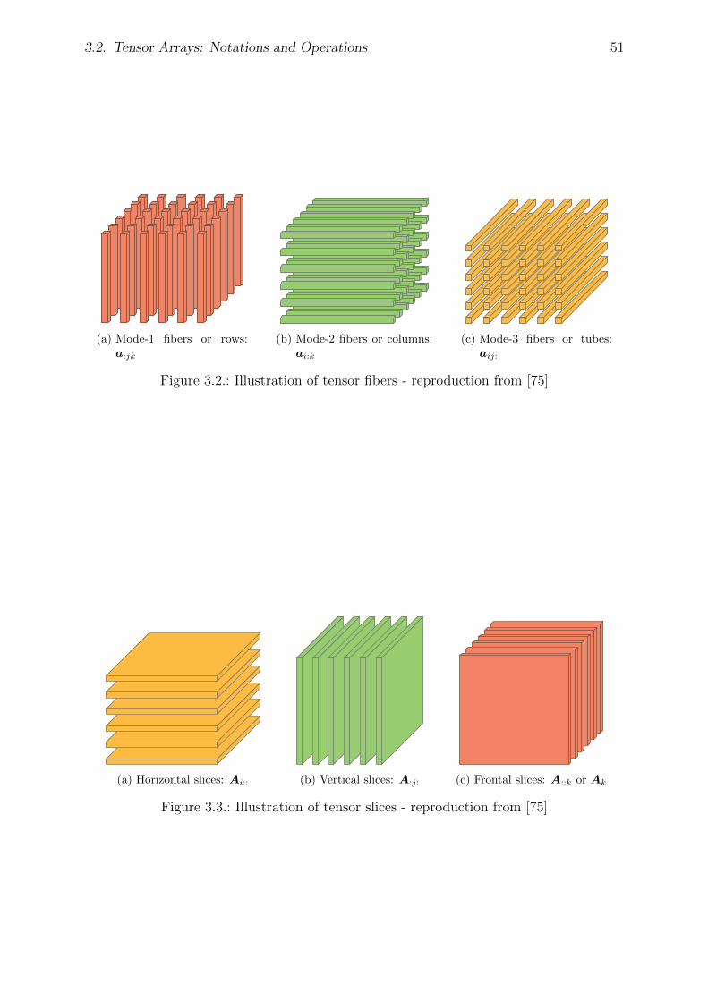
3.2. Tensor Arrays: Notations and Operations 51

(a) Mode-1 fibers or rows:a:jk

(b) Mode-2 fibers or columns:ai:k

(c) Mode-3 fibers or tubes:aij:

Figure 3.2.: Illustration of tensor fibers - reproduction from [75]

(a) Horizontal slices: Ai:: (b) Vertical slices: A:j: (c) Frontal slices: A::k or Ak

Figure 3.3.: Illustration of tensor slices - reproduction from [75]


1. Fibers are obtained by fixing all indices except one: fibers are always representedby column vectors. Rows a:jk are mode-1 fibers (in Figure 3.2a), whereas columnsai:k are mode-2 fibers (in Figure 3.2b). Moreover, tubes aij: are mode-3 fibers (inFigure 3.2c).

2. Slices are obtained by fixing all but two indices, i.e. slices are 2D sections of atensor: Ai:: (“horizontal” slices, in Figure 3.3a), A:j: (“vertical” slices, in Figure3.3b) and A::k(“frontal” slices, in Figure 3.3c). Alternatively, the k-th “frontal”slice can be represented by the more compact form Ak.

Definition 3.3. The inner product between two tensors of the same size: X ,Y ∈CI1×···×ID :

< X ,Y >=

I1∑i1=1

· · ·ID∑iD=1

Xi1···iD Y∗i1···iD (3.5)

with associated Frobenius norm ‖X‖ =√< X ,X >.

Definition 3.4. A tensor X ∈ CI1×···×ID is diagonal if Xi1···iD 6= 0⇔ i1 = i2 = · · · = iD,i.e. it has non zero elements only on its diagonal.

It is often useful to store the elements of aD-way array into a matrix, through unfoldingsor flattenings, depending on the arbitrary order choice. The most used matricizations aregiven by the mode-d unfoldings, i.e. matrices whose number of rows equals the d-th tensordimension [26, 75]:

Definition 3.5. The mode-d unfolding of a tensor X ∈ CI1×···×ID is denoted by X(d) andarranges the mode-d fibers as columns of the resulting matrix.

It is easily verified that the Frobenius norm of any unfolding is equal to the tensor normin Definition 3.3:

‖X‖ = ‖X(d)‖, ∀d (3.6)

Reformatting of tensors in general is called reshaping. Through the reshaping operationwe can unvectorize a tensor, as the reverse of the vectorization operation [22]. For example,in 2D we have the following vec· and unvec· operations:

Definition 3.6. The vectorization of a matrix X = [x1, . . . ,xJ ] ∈ CI×J stacks itscolumns (or mode-2 fibers) xj into a vector:

x = vecX = [xT1 , . . . ,x

TJ ]T ∈ CIJ

x(i−1)J+j = Xij

(3.7)

Through the reshape operation (similar to the reshape MATLAB function) we canrecover the original matrix X:

reshape(x, I, J) = [x(1 : I),x(I + 1 : 2I), . . . ,x(IJ − I + 1 : IJ)] ∈ CI×J (3.8)

For higher order tensors, we can define a similar vectorization operation. We define itfor D = 3, but it is easily extended to higher order tensors [22]:

3.2. Tensor Arrays: Notations and Operations 53

Definition 3.7. The vectorization of a tensor X ∈ CI×J×K is defined as the vectorizationof the associated mode-1 unfolding X(1) ∈ CI×JK . Hence, it stacks all its mode-1 fibersx:jk into a vector:

x = vecX = vecX(1) = [vecX ::1, · · · , vecX ::K]T

= [xT:11,x

T:21, . . . ,x

T:J1, . . . ,x

T:1K ,x

T:2K , . . . ,x

T:JK ]T ∈ CIJK

(3.9)

We adopt the usual definition [10] where the vec· operation takes indices in lexico-graphical order. Then we have the identity [10, 75]: vecabT = b a, for any pair ofvectors (a, b). More generally:

veca⊗ b⊗ c = c b a

veca(1) ⊗ · · · ⊗ a(D) = a(D) · · · a(1)(3.10)

N.B. Although there exists an objectively better definition [24], allowing to preserve theorder of the products, it is rarely used in the literature.

3.2.3. Multi-Way Operations

We define two fundamental operations, increasing and decreasing tensor order, respec-tively. Tensor product increases order D:

Definition 3.8. The tensor product A ⊗ B between tensor A = [Aij] ∈ S1 ⊗ S2 andtensor B = [B`m] ∈ S3 ⊗ S4 is tensor C = [Cij`m = AijB`m] ∈ S1 ⊗ S2 ⊗ S3 ⊗ S4

An example of tensor product is the outer product of two vectors a ∈ CIa and b ∈ CIb :a⊗ b = abT ∈ CIa×Ib . Notice that the outer product of multiple vectors is a higher ordertensor: a(1) ⊗ a(2) ⊗ · · · ⊗ a(D) ∈ CI1×···×ID , whereas the Kronecker product of multiplevectors remains a vector: a(1) a(2) · · · a(D) ∈ CI1···ID .

Definition 3.9. The contraction or mode-d product •d between tensor A of order D andtensor A′ of order D′ consists in a summation over a pair of indices. The result is a tensorB = A •d A′ of order D +D′ − 2.

For (D,D′, d) = (3, 3, 2)

Bijpq =∑`

Ai`j A′p`q (3.11)

Matrix multiplication is an example of mode-1 product between two matrices, B =AA′ = AT •1A

′, with Bim =∑

ÀiÀ′`m. When the mode-d product is between a matrix

U ∈ CJ×Id and a higher order tensor X ∈ CI1×···×ID , as a rule, we sum over the secondindex of the matrix,

(X •d U)i1···id−1jid+1···iD =

Id∑id=1

Xi1···iDUjid (3.12)

This can also be expressed in terms of unfolded tensors: Y = X •d U ⇔ Y (d) = UX(d).As an example, the mode-3 product A •3 M between a matrix and a third order tensorgives the third order tensor: Bipq =

∑`MiÀpq`.

A natural extension of the mode-d product is the following:


Definition 3.10. The multilinear product of a tensor with each matrix of a list A =A(1), . . . ,A(D), where A(d) ∈ CJd×Id is a set of D independent mode-d products. Alter-natively, we can express a multilinear product through unfoldings and Kronecker products:

Y = X •1 A(1) •2 A

(2) · · · •D A(D) ⇔

Y (d) = A(d)X(d)

(A(D) · · ·A(d+1) A(d−1) · · ·A(1)

)T (3.13)

When a tensor defines a multilinear operator, the mode-d product with a matrix isrelated to a change of basis, through multilinear product [26]. For D = 3 we have threeindependent mode-d products:

Proposition 3.1. If a linear change of basis is made in S1, S2, and S3 (x′ = Ax,y′ =By, z′ = Cz), then the array T ′ defining the multilinear map f in the new coordinatesystem is a function of T :

X ′ = (A,B,C) ·X = X •1 A •2 B •3 C

X ′ijk =∑

pqr AipBjq Ckr Xpqr(3.14)

We recall then the definition of a tensor in relation to multilinear changes of bases:

Definition 3.11. A tensor of order D is an element of S1 ⊗ · · · ⊗ SD, and can be rep-resented by a D-way array once bases of spaces Sd have been fixed. Under multilineartransformations, the array of coordinates changes according to (3.14).

3.3. Tensor Decompositions

3.3.1. Decomposable Tensors and Tensor Rank

M =

M =

a

b

c

a⊗ b⊗ c

Figure 3.4.: A decomposable third order tensor - reproduction from [75]

The tensors of order D spanning the corresponding tensor space as defined in Definition3.2 are very characteristic: they can be decomposed into an outer product of D vectors.Figure 3.4 illustrates a decomposable tensor of order D = 3. This leads us to the followingdefinition:

Definition 3.12. A decomposable tensor, or rank-1 tensor, is given by the outer productof vectors: D = a⊗ b⊗ · · · ⊗ c, with elements Dij...k = aibj · · · ck.

3.3. Tensor Decompositions 55

Decomposable tensors correspond to the discretization of a function of D separablevariables (see Section 3.7 for more details).

Proposition 3.2. Any tensor T can be decomposed into a linear combination of Rdecomposable tensors D(r):

M =R∑r=1

ςrD(r) (3.15)

where coefficients ςr can be always chosen to be real positive, and decomposable tensorsD(r) to have unit norm, i.e. the product ‖a(r)‖ ‖b(r)‖ · · · ‖c(r)‖ = 1, but other choicesare possible (cf. Section 3.3.4).

Definition 3.13. The minimum value R for which (3.15) holds is called tensor rank.

Unlike matrix rank, tensor rank may exceed all dimensions and depends on the choicefor field K.

In the remainder, we will generally state results for 3-order tensor decompositions. Thegeneralization to D-order tensors is straightforward.

3.3.2. Tucker Decomposition and Multilinear Rank

The Tucker Decomposition (TKD) is a form of higher order principal component analysis.

Definition 3.14. The TKD M = (A,B,C) · G = G •1 A •2 B •3 C is given by amultilinear transformation of a dense but typically small core tensor G ∈ CP×Q×R:

M =∑P

p=1

∑Qq=1

∑Rr=1 Gpqr ap ⊗ bq ⊗ cr

Mijk =∑

p

∑q

∑r Gpqr AipBjq Ckr

(3.16)

The columns of factor matrices A ∈ CI×P , B ∈ CJ×Q and C ∈ CK×R represent theprincipal components along each mode, whereas the entries of the core tensor describeinteractions between the components. The term on the left of (3.16) refers to the i, j, kentry of the multi-way array, so that a total number of I × J ×K terms are known. Theterm on the right indicates the number of unknowns: (P × Q × R) + IP + JQ + KR.If the number of unknowns is smaller than the number of equations, there will generallybe no solution. This is the case when both core tensor G is diagonal and factor matricesA, B and C are orthonormal. R1 = P refers to the row rank, i.e. the dimension of thespace spanned by mode-1 fibers; R2 = Q refers to the column rank, i.e. the dimension ofthe space spanned by mode-2 fibers, and so on. For D ≥ 3, R1, . . . , RD can be different.For generic D, we have:

Definition 3.15. The d-rank of tensor M ∈ CI1×···×ID is the dimension of the vectorspace spanned by its mode-d fibers:

Rd = rankdM = column rank of M (d) ≤ Id (3.17)

The D-tuple (R1, . . . , RD) is called the multilinear rank of tensor M.

If we only apply the orthonormality constraint to (3.16), we obtain HOSVD [26]. Ifwe only keep a diagonal core tensor, we obtain the polyadic decomposition defined inSection 3.3.3. TKD is used to compress data or to find the D sub-spaces spanned by the


tensor fibers. On the other hand, the polyadic decomposition is used to factorize datainto components easy to interpret. Thus, there exist two main instances of constrainedTKD, with factor orthonormality or diagonal core constraints: HOSVD of Definition 3.18and the polyadic decomposition of Definition 3.17.

Definition 3.16. The multilinear SVD or High Order Singular Value Decomposition(HOSVD) consists in a TKD with orthonormal factor matrices:

M = S •1 U 1 •2 U 2 •3 U 3 (3.18)

We can derive factor matrices U d via the SVD of mode-d unfoldings M (d) = U dΣdVHd .

The columns of factor matrices U d are interpreted as multilinear singular vectors, and thenorm of the slices of the core are multilinear singular values, these slices being mutuallyorthogonal.

3.3.3. Canonical-Polyadic Decomposition (CPD) and Tensor Rank

Consider the expression in (3.15), defining the tensor rank, as any tensor can be decom-posed into a sum of rank-1 tensors. For D = 3, it takes the form below:

M =R∑r=1

ςr a(r)⊗ b(r)⊗ c(r) (3.19)

We denote Air, Bjr and Ckr the coordinates of vectors a(r) in basis e(1)i , b(r) in basis

e(2)i , and c(r) in basis e

(3)i respectively. Then, M can be expressed as

M =R∑r=1

ςr

(I∑i=1

Aire(1)i

)⊗(

J∑j=1

Bjre(2)j

)⊗(

K∑k=1

Ckre(3)k

)=

=∑ijk

(R∑r=1

ςr Air Bjr Ckr

)e

(1)i ⊗ e(2)

j ⊗ e(3)k

(3.20)

From (3.4), we derive the basis-dependent expression of array coordinates in (3.21), asrepresented in Figure 3.5:

Definition 3.17. The Polyadic decomposition is indicated by M = (A,B,C) · L =L •1 A •2 B •3 C where R×R×R core tensor L = Diagς is diagonal:

M =∑R

r=1 ςr ar ⊗ br ⊗ crMijk =

∑Rr=1 ςr Air Bjr Ckr

(3.21)

where L = Diagς is diagonal, and ς = [ς1, . . . , ςR]T.

Notice that the Polyadic Decomposition in (3.21) is equivalent to (3.15) in terms ofarray coordinates, thus revealing tensor rank1. If R is not too large, this decompositionis unique (up to the equivalence relation of Definition 3.2) and is referred to as CanonicalPolyadic Decomposition (CPD) (see [135, 26] and references therein. Uniqueness, whichis the main motivation in resorting to tensors, will be treated in Section 3.3.5 .

1The problem of estimating the rank of a given tensor is NP hard. In practice, it is often determinednumerically by fitting different rank-R CPD models [75].


M =

M =

ς1

a1

b1

c1

ς1 a1 ⊗ b1 ⊗ c1

+ [· · · ] +

+ [· · · ] +

ςR

aR

bR

cR

ςR aR ⊗ bR ⊗ cR(a) CPD as a sum of rank-1 terms

I × J ×K

M =A

I ×R

L

R×R×R

BT

R× J

C

K ×R

M = L •1 A •2 B •3 C(b) CPD as a linear change of basis

Figure 3.5.: Illustration of the CPD of a 3-order tensor - reproduction from [22]


It is often useful to express the CPD of a D-order tensor M through tensor unfoldingsand vectorization [21]:

M = (A(1), . . . ,A(D)) ·L =∑R

r=1 ςr a(1)r ⊗ · · · ⊗ a(D)

r

M (n) = A(n)L(A(D) . . .A(n+1) A(n−1) . . .A(1))T

vecM = (A(D) . . .A(1))ς =∑R

r=1 ςr a(D)r · · · a(1)

r

(3.22)

For D = 3 and ςr = 1 ∀r, we have three mode-d unfolding representations of CPD [75]:M (1) = A(C B)T

M (2) = B(C A)T

M (3) = C(B A)T(3.23)

Moreover, when D = 3, we can express CPD in terms of “frontal” (or “horizontal”, or“lateral”) slices:

M ::k = ADk(ck:)BT where Dk(ck:) = Diagck:

M :j: = ADj(bj:)CT where Dj(bj:) = Diagbj:

M i:: = BDi(ai:)CT where Di(ai:) = Diagai:

(3.24)

For simplicity, “frontal” slices can be expressed merely by M k = M ::k.

3.3.4. CPD Factors, Normalization and Scaling

A CPD is said to be essentially unique if there exist a unique set ςr, D(r), 1 ≤ r ≤ Rsuch that equality holds in (3.15). However, even if the CPD is unique, there exist severalways of writing (3.15). In fact, writing a decomposable tensor as the outer productof vectors is subject to scaling indeterminacies, which actually stem from multilinearityproperties of tensors [26], since

αa⊗ βb⊗ γc = a⊗ b⊗ c (3.25)

if αβγ = 1. Even if the above vectors are of unit Euclidean norm, there remain twoscaling indeterminacies of unit modulus. As a consequence, attention should be paid tothe difference between CPD or essential uniqueness, and uniqueness of factor matricesappearing in (3.21).

The trivial indeterminacies intrinsic in the array representation (3.21), M =(A,B,C) · I, are of two orders:

1. Arbitrary scaling of components for any R × R invertible diagonal matrices∆1,∆2,∆3 satisfying ∆1∆2∆3 = I:

M = (A∆1,B∆2,C∆3) · I (3.26)

or, equivalently,

M =R∑r=1

(αrar)⊗ (βrbr)⊗ (γrcr) with αrβrγr = 1 ∀r (3.27)


2. Permutation of the rank-1 terms, for any R×R permutation matrix Π:

M = (AΠ,BΠ,CΠ) · I (3.28)

In practice, it is more convenient to fix the trivial indeterminacies of unit modulus in(3.21). It is often common to assume that the columns of factor matrices A, B, andC, have unit norm, with the weights absorbed into vector ς = [ς1, . . . , ςR]. As suggestedin [128], for a D-order CPD, we generally fix (D − 1)R parameters without restrictingthe generality (cf. Sections 4.3.1, 5.3.4, 5.4.1, and 6.4 for examples of physics relatedconstraints).

3.3.5. Uniqueness of the CPD

The unconstrained TKD is not unique, as factor matrices are rotation invariant:

(A,B,C) · G = (AU−1,BV −1,CW−1)(G •1 U •2 V •3 W ) (3.29)

However, the subspaces spanned by factor vectors are unique [21], even though we mightsimplify the core structure as sparse or orthogonal, thus minimizing the interactions be-tween components.

In order to better understand the interest of tensor CPD, we illustrate the case ofrank-R tensor decompositions of order two, which are not unique. This is the model usu-ally employed in Blind Source Separation (BSS) and Non Negative Matrix Factorization(NMF) [21]:

M =R∑r=1

ςr ar ⊗ br =R∑r=1

ςr arbTr = ALBT (3.30)

where L = Diagς1, . . . , ςR ∈ CR×R is a normalizing matrix, the columns of B representthe unknown sources, and the columns of A represent the associated mixing vectors, asrepresented in Figure 3.6. It is clear that, when D = 2 (the multi-way array is a matrix),if model (3.30) is unconstrained, it admits infinite combinations of A and B: AT , BT ,where T is orthogonal, i.e. T T = T−1. For example, if the SVD of M is UΣV T, we canchoose A = UΣT , and B = V T . Therefore, uniqueness is attained thanks to restrictiveconstraints such as orthogonality (EVD and SVD) or triangularity (QR factorization),statistical independence, nonnegativity, etc. (cf. [22] for details). For example, the SVDis generically unique because U and V are orthonormal, and Σ is diagonal [75]. On theother hand, the CPD of tensors of order D ≥ 3 is unique under mild conditions.

A necessary condition for uniqueness for CPD is that the number of equations be at leastas large as the number of unknowns: for a tensor of order D and dimensions I1×· · ·× ID,we have (

D∑d=1

Id −D + 1

)R ≤

D∏d=1

Id (3.31)

(3.31) induces an upper bound on tensor rank, the expected rank R0:

R ≤ R0 =

∏D

d=1 Id(∑Dd=1 Id −D + 1

) (3.32)

Notice that we subtract (D − 1)R degrees of freedom because, in order to fix scalingindeterminacies, we fix (D − 1)R terms (see Section 3.3.4).


M =

M =

ς1

a1

b1

ς1 a1 bT1

+ [· · · ] +

+ [· · · ] +

ςR

aRaR

bR

ςR aR bTR

(a) CPD as a sum of rank-1 terms

M =

I × J

A

I ×R

L

R×R

BT

R× J

M = ALBT

(b) CPD as a linear change of basis

Figure 3.6.: Illustration of the CPD of a matrix - reproduction from [22]

The typical rank is any rank that occurs with probability greater than zero (this prob-ability is generally estimated through MC experiments that randomly draw each entryfrom a continuous distribution).

For I × J matrices, the expected and typical ranks are equal to minI, J, whereas fortensors they may differ, and there may be more than one typical rank in R (in C there isonly one typical rank). If only one typical rank exists, it occurs with probability one andis called generic [27].

In general, only the weak upper bound on the rank of a third order tensor is known[82]:

rankM ≤ minIJ, JK, IK (3.33)

A sufficient condition for the uniqueness of the CPD has been given by Kruskal for 3-wayarrays [81, 26, 21]:

2R + 2 ≤ κA + κB + κC (3.34)

and was later generalized to D-way arrays by [135]:

2R +D − 1 ≤D∑d=1

κd (3.35)

where κd denotes the Kruskal rank of the d-th factor matrix of the CPD. This conditionis also necessary for D = 2, 3 [75].

Definition 3.18. The Kruskal rank of a matrix A, κ(A), is the largest number κ suchthat any combination of κ columns is full rank. Therefore, κ(A) ≤ rankA.

3.4. Multilinear Normal Distributions 61

A necessary condition for (3.35) to hold is that D ≥ 3 [88]. However, less stringentconditions guaranteeing almost surely a unique solution can be found, for instance, in[88, 26, 19]:

R(I + J +K − 2) < IJK (3.36)

i.e. if R < R0, or in [31]:

R ≤ K and R(R− 1) ≤ I(I − 1)J(J − 1)

2(3.37)

Notice that (3.36) and (3.37) are both valid for D = 3.

Tensor uniqueness conditions are milder and more natural, compared to matrix factor-izations, as they only require the components to be sufficiently diverse and their numbernot too large. Sometimes prior knowledge of data properties, such as statistical indepen-dence, sparsity, Vandermonde structure, non negativity and orthogonality can be used asconstraints to relax the uniqueness condition of CPD [21].

3.3.6. Advantages of the Tensor Formalism when D ≥ 3

We enumerate hereafter some of the advantages offered by multilinear algebra tools.

1. Tensors are multi-way arrays that admit a compact representation and are typi-cally overdetermined, i.e. the number of equations is greater than the number ofunknowns. This enhances the robustness to noise and to missing data.

2. Tensor methods are able to directly operate on raw data, with no need to estimatehigher order statistics: they can be considered deterministic and can deal with dataof very short duration.

3. Flexibility in the choice of constraints, with less restrictive conditions than orthonor-mality or triangularity.

4. Uniqueness of decompositions under milder assumptions.

3.4. Multilinear Normal Distributions

Let x be a I × 1 vector of random variables from a standard normal distribution, x ∼N (0, I), and y = Ux its linear transformation through a non singular I × I matrix U .Then, y ∼ N (0,Σ), where Σ = UUH.

Now let X be a I1× I2 random matrix, and Y = U 1XUT2 = X •1U 1 •2U 2 its bilinear

transformation through non singular matrices U 1 ∈ CI1×I1 and U 2 ∈ CI2×I2 . Then,Cov[Y ] = Σ1 ⊗ Σ2, where Σj = U jU

Hj , j = 1, 2. This covariance is said separable, as

it can be divided into a row covariance Σ1 and a column covariance Σ2. If the elementsof X follow a standard normal distribution, then the bilinearly transformed matrix Yfollows a matrix zero mean normal distribution: Y ∼ N (0,Σ1 ⊗Σ2).

Let us increase the dimension and generalize this to random arrays. We introduce thedefinition of tensor multivariate normal distribution [67]:


Definition 3.19. We say that the multivariate random variable X ∈ CI1×I2×···×ID followsan array Gaussian distribution of mean M and covariance C = Σ1⊗· · ·⊗ΣD ∈ CI1×I1⊗· · · ⊗ CID×ID , a tensor of order 2D, and we write X ∼ AN (M,C)2, if

p (X |M,Σ1, . . . ,ΣD) = (2π)−I/2|C|−1/2exp

(−∥∥∥(X −M) • C−1/2

∥∥∥2/2

)(3.38)

with I =∏D

d=1 Id, and C−1/2 = Σ−1/21 , . . . ,Σ

−1/2D , and |C|−1/2=

∏Dd=1 |Σd|−I/(2Id).3

Definition 3.20. The covariance C of a multivariate random variable X ∈ CI1×I2×···×ID

is said separable, since it can be expressed as the outer product of matrices Σd: C =Σ1 ⊗ · · · ⊗ΣD [67].

Definition 3.21. The I1 × I2 × · · · × ID array X ∼ AN (0, II1 ⊗ · · · ⊗ IID) is said to bestandard Gaussian.

If we apply a multilinear transformation U 1, · · · ,UD on tensor X =∑R

r=1 a(1)r ⊗

· · · ⊗ a(D)r , its CPD nature is not modified:

Y = (U 1, · · · ,UD) ·X =R∑r=1

U 1 a(1)r ⊗ · · · ⊗UD a

(D)r (3.39)

Thus, the CPD is stable under multilinear transformations.

Similarly, we state the following results for the effects on the covariance structure aftermultilinear transformation of a random multi-way array [67]:

Proposition 3.3. If Cov[X ] = Σ1 ⊗ · · · ⊗ΣD and Y = X •dG, then

Cov[Y ] = Σ1 ⊗ · · · ⊗Σd−1 ⊗(GΣdG

T)⊗Σd+1 ⊗ · · · ⊗ΣD (3.40)

This implies that the class of separable covariance arrays is stable under the action ofmode-d products. More generally,

Proposition 3.4. Let X ∼ AN (M, II1 ⊗· · ·⊗ IID) and U 1, . . . ,UD be a multilineartransformation, and Σd = U dU

Hd . Then, the multilinear product

Y = (U 1, · · · ,UD) ·X has the following properties:

1. E[Y ] = (U 1, · · · ,UD) · E[X ]; Cov[Y ] = Σ1 ⊗ · · · ⊗ΣD

2. E[Y (d)] = U (d) E[X(d)] (U (D) . . .U (d+1) U (d−1) . . .U (1))T;E[Y (d)Y

H(d)] = Σd

∏i 6=d traceΣi

3. E[vecY] = (UD · · ·U 1)E[vecX]; Cov[vecY] = ΣD · · ·Σ1

Moreover, the probability density of Y , vecY,Y (d), remain Gaussian.

2AN denotes Array Normal.3We recall that, as in Definition 3.10, the multilinear product between a tensor X of order D and

a collection of matrices A = A1, . . . ,AD is defined as a set of D independent mode-d products:X •A = X •1 A1 · · · •D AD.

3.5. Algorithms for Exact Decompositions 63

3.5. Algorithms for Exact Decompositions

We recall the expression (3.21) of the R-term trilinear model for the 3-way array M:M =

∑Rr=1 ςr ar ⊗ br ⊗ cr

Mijk =∑R

r=1 ςr Air Bjr Ckr(3.41)

We shall describe an algebraic approximate solution for the exact CPD4, though jointdiagonalization of two matrices.

3.5.1. Computation of the CPD through Joint Diagonalization

A direct decomposition algorithm has been proposed in [85]: it takes as inputs the Kmatrix slabs M k = M ::k and the number of factors R, and returns the estimates ofmatrices A, B and C. The uniqueness of such a solution is guaranteed provided that theR column vectors corresponding to two of the ways are linearly independent, and the Rcolumn vectors associated with the third way have the property that no two are collinear(see below). The trilinear model (3.41) can be rewritten as K slices M k of size I × J ,according to (3.24):

M k =R∑r=1

(ar ⊗ br)Ckr =R∑r=1

ar Ckr bTr = ADk(ck:)B

T (3.42)

where Dk(ck:) = Diagck: and coefficients ςr were pulled in factor matrix B.The following more constraining identifiability conditions are employed, which concur-

rently imply the Kruskal condition in Equation (3.34):

IC1 The columns of A are linearly independent i.e. κA = R.

IC2 The columns of B are linearly independent i.e. κB = R.

IC3 Every pair of columns of C is linearly independent i.e. κC = 2.

Each condition refers to one way of the array: the first two conditions state that theremust be at least R factors present in two ways. The third requires that no two factorsare linked by a proportional relationship along the other way.

The decomposition proposed in [85] exploits the comparison between the two followinglinear combinations, for every vector of weights ρ ∈ RK :

M (ρ) =∑K

k=1 ρkM k

C(ρ) =∑K

k=1 ρkDk(ck:)(3.43)

As particular combination we denote M+ =∑K

k=1M k and C+ =∑K

k=1Dk(ck:). Thefollowing result constitutes the theoretical basis of the decomposition algorithm (see [85]for more details on its implementation):

Theorem 3.1. If conditions IC1 and IC2 hold, A and B have a left inverse and

1. the columns of matrix A are the eigenvectors of the matrix M (ρ)M †+; the corre-

sponding eigenvalues are the diagonal entries of C(ρ)C−1+ .

4Exact is intended as in the absence of additive noise


2. matrix B can be obtained as B = (C−1+ A

†M+)T;

3. the columns of matrix C can be obtained thanks to the relation Dk(ck:) =A†M k(B

T)†.

Sketch of proof. From (3.42), we have M k = ADk(ck:)BT, and M+ = AC+B

T. Hencefor any k, M kM

†+A = ADk(ck:)C

−1+ .

3.6. Tensor Approximation

3.6.1. An Approximation Problem in Additive Noise

In practice, we admit that observations X , related to the model M, are corrupted by anadditive noise N . In other words, the observation model becomes X = M+N , and thegoal is to fit (3.22) with the data. In any case, when the data are noisy, the fit alone cannotdetermine the rank [75]. In practice, the presence of noise requires a fit of a multilinearmodel of lower rank, i.e. with R < rankX, leading to an approximation problem. Thefact that the set of rank-R tensors is not closed when R > 1 may raise difficulties (seeSection 3.6.2 for the question of existence of a rank-R approximant). The reasons whywe cannot resort to an exact decomposition with R = rankX is that generally, the realrank R is unknown and that decompositions with larger rank are not unique [27] (seeSection 3.3.5 for the question of uniqueness).

Data tensor have a normal distribution under the following assumption:

A 3.1. Additive noise follows an array normal distribution with zero mean: N ∼ N (0,C).It follows that X ∼ N (M,C), where M has a CPD structure.

The approximation problem of a tensor X ∈ CI×J×K through a CPD with R compo-nents is given by

minX‖X − X‖ = min

A,B,C

∥∥∥∥∥X −R∑r=1

ςr ar ⊗ br ⊗ cr∥∥∥∥∥

2

C

(3.44)

where C indicates the covariance of tensor X , after defining the weighted tensor norm‖X‖C = ‖C−1/2 •1 •2 •3 X‖.

The cost function (3.44) can be expressed via unfoldings X(1) ∈ CI×JK , X(2) ∈ CJ×IK ,and X(3) ∈ CK×IJ :

minX(1)‖X(1) − X(1)‖ = minA,B,C

∥∥∥X(1) − A(C B)T∥∥∥2

C(1)=

minX(2)‖X(2) − X(2)‖ = minA,B,C

∥∥∥X(2) − B(C A)T∥∥∥2

C(2)=

minX(3)‖X(3) − X(3)‖ = minA,B,C

∥∥∥X(3) − C(B A)T∥∥∥2

C(3)

(3.45)

where C(d) represents the covariance of the mode-d unfolding.Alternatively, (3.44) can be expressed through vectorization x = vecX:

minx‖x− x‖ = min

A,B,C

∥∥∥∥∥x−R∑r=1

ςr cr br ar

∥∥∥∥∥2

Σ(1)

(3.46)

3.6. Tensor Approximation 65

where Σ(1) represents the covariance of tensor vectorization x. Analogously, we define

the weighted matrix norm as ‖X‖Σ =√

traceXHΣ−1X.In the remainder, unless otherwise specified, we will make the following assumption:

A 3.2. Additive noise is white Gaussian, i.e. its variance C is diagonal: C = σ2II×J×K .It follows that the noise of tensor unfoldings and vectorization also have a diagonal co-variance: C(1) = σ2II×JK , C(2) = σ2IJ×IK , and C(3) = σ2IK×IJ ; Σ(1) = σ2IIJK .

Notice that, if Assumption A 3.2 is verified, the weighted norms ‖ · ‖C and ‖ · ‖Σ reduce

to simple Frobenius norms ‖X‖ =√< X ,X > and ‖X‖ =

√traceXHX.

The Cramer-Rao Bound (CRB) for the CPD approximation problem in additive i.i.d.complex circularly symmetric Gaussian noise was derived in [90, 149].

3.6.2. Existence and Degeneracies

For matrices, Eckart and Young [39] showed that a best rank-k approximation, withk ≤ R, is given by the first k leading singular vectors of the SVD X =

∑Rr=1 ςr ur ⊗ vr.

This means that the rank-k approximation A minimizing ‖X −A‖2 is given by

A =k∑r=1

ςr ur ⊗ vr (3.47)

This result is not true for higher order tensors: the existence of the best rank-k ap-proximant is not guaranteed. As a consequence, all the factors of a rank-k approximationmust be found simultaneously [75]. This problem leads to the definition of degeneracy :

Definition 3.22. A tensor is said degenerate if it may be approximated arbitrarily wellby a factorization of lower rank.

In the case of degeneracy, although reducing the approximation error, some rank-1factors become close to proportional, and the magnitude of some terms goes to infinity,with opposite signs. The best rank-k approximation is on the boundary of the space ofrank-k and rank-k+1 tensors. Since the space of rank-k tensors is not closed, the sequenceof arbitrarily better rank-k approximant tensors can converge to a tensor of rank k + 1.Hence, the infimum of the approximation problem in (3.44) may never be reached; werefer to [88, 27] for further details.

Imposing non negative constraints on the tensor model is a way to prevent degeneracy,as cancellation of opposite diverging rank-1 tensors cannot occur when tensors have pos-itive entries only [87]. On the other hand, if tensor entries are free and R > 1, one mightperform the minimization over a closed subset, or by adding a regularization term to theobjective function in (3.44) (see [128] for an example).

Alternatively, one might also adopt a closed superset, such as the adherence of rank-Rtensors. In light of this fact, it is useful to define the concept of border rank:

Definition 3.23. The border rank of a tensor X corresponds to the minimum numberof rank-1 tensors that approximate X with arbitrarily small nonzero error:

rankX = minr : ∀ε > 0 ∃ E s.t.‖E‖ < ε and rankX + E = r (3.48)

We always have: rankX ≤ rankX.


3.6.3. Algorithms for Tensor Approximation

All the algorithms proposed in the literature aim at minimizing the fitting error in (3.44).References can be found in [27]. Before resorting to tensor approximation algorithms, di-mension reduction through HOSVD is often recommended, both for speed of convergenceand computational complexity, provided that the tensor dimensions are not smaller thanthe rank R chosen for the decomposition [27]. In particular, since the core S of HOSVDin (3.18) is all orthogonal, we can calculate the truncated HOSVD [32], which gives agood starting point for the Alternating Least Squares (ALS). The truncation discards themultilinear singular vectors and slices in the core tensors corresponding to the smallestmultilinear singular values.

Gradient descent

We can express the cost function in (3.44) through parameter vectorization, Υ = Υ(ϑ),where ϑ = [vecA, vecB, vecC]T. Hence, the iteration is given by

ϑ(k + 1) = ϑ(k)− µ(k)∇Υ(ϑ)|ϑ=ϑ(k) (3.49)

where µ is the iteration dependent stepsize.The gradient descent is the simplest algorithm, but with very poor convergence be-

haviour. However, it can be improved through Enhanced Line Search (ELS) or throughthe Levenberg-Marquardt algorithm [27]. ELS in particular is more robust to the presenceof local minima and more efficient than simple gradient descent.

Alternating Least Squares

Alternating Least Squares (ALS) can be seen as an example of non linear LS problem,where variables separate [27]. We present the ALS method only for D = 3 throughunfoldings (3.23). However, it is easily generalized to any D through (3.22).

The idea is to obtain a quadratic function of one factor matrix, while keeping the otherfactor matrices fixed: for instance, for D = 3, we fix B and C, and we solve for A,alternatively, until convergence of a given criterion. We have then the quadratic form

minA‖X(1) − A(C B)T‖2 (3.50)

where we store weights in A = ADiagς. The solution to (3.50) is given by

A = X(1)[(C B)T]† =

X(1)(C∗ B∗)(CTC∗ BTB∗)−1

(3.51)

Finally, we normalize the columns of A to get A: ςr = ‖ar‖ and ar = ar/ςr. If (CB)T

has full column rank, (3.51) is the LS solution of the over-determined linear system.The ALS algorithm for generic D is described in Algorithm 3.1. The factor matrices

can be initialized through the HOSVD:

A(d) ← R leading left singular vectors of X(d) (3.52)

ALS is very easy to implement, but can take many iterations and is not guaranteedto converge to a global minimum nor a stationary point. It may depend strongly oninitialization [75]. It has a satisfactory performance for high SNR, and for well separatedcomponents (cf. Section 3.7 for a measure of separateness).

3.7. Physical Diversity and Coherence 67

Algorithm 3.1 CP ALS

1: Inputs:

• Initialize with A(d) ∈ CId×R, 1 ≤ d ≤ D.

• Data tensor X ∈ CI1×···×ID .

2: While convergence criterion not met, do k := k + 13: for d = 1, . . . , D do4:

V ← A(1)TA(1)∗ · · ·A(d−1)TA(d−1)∗ A(d+1)TA(d+1)∗ · · ·A(D)TA(D)∗

A(d) = X(d)(A(D)∗ · · · A(d+1)∗ A(d−1)∗ · · · A(1)∗)V −1

(3.53)Normalize columns of A(d), storing their norms in ς

5: end for6: Outputs:

• Factor matrices A(d), 1 ≤ d ≤ D.

• Coefficient vector ς.

7: End

Other methods

An interesting semi-algebraic solution for approximate CPD via simultaneous joint diag-onalizations can be found in [121].

3.7. Physical Diversity and Coherence

As we will develop in Section 5.2, many physical phenomena can be modeled through twofundamental concepts: sparsity (sum of simpler constituents) and separability (separationof variables). The underlying model is then expressed through a D-partite target functionf : S1 × · · · × SD 7−→ C:

f(x1, ...,xD) =R∑r=1

ςr

D∏d=1

φrd(xd), ςr ∈ C,∀r (3.54)

For D = 3, we have f : S1 × S2 × S3 7−→ C:

f(x,y, z) =R∑r=1

ςr ar(x) br(y)cr(z) (3.55)

If we discretize (3.55), we obtain a tensor array:M =

∑Rr=1 ςr ar ⊗ br ⊗ cr

Mijk =∑R

r=1 ςr Air Bjr Ckr(3.56)

with Mijk = f(xi,yj, . . . ,zk), Air = ar(xi), Bjr = br(yj) and Ckr = Cr(zk), and vectorsar = [A1r, . . . , AIr]

T, br = [B1r, . . . , BJr]T, and cr = [C1r, . . . , CKr]

T. Notice that the


discretization of a sparse and separable function in (3.56) is equivalent to the CPD in(3.21). Namely, separability of a continuous function is equivalent to the discrete conceptof rank-1 or decomposable tensor, when subsets S1, . . . ,SD are finite sets.

In the continuous case, the domain Ω of function f is generally constrained throughdifferentiability or integrability (C∞(Ω) or L2(Ω)), whereas in the discrete case Ω =CI1×···×ID . The requirement D ≥ 3 for identifiability of CPD in (3.15) implies that our datamust be at least a 3-way array in the discrete case as in (3.56), and that the underlyingmodel must be a function of at least three variables in the continuous case, i.e. a D-partite or multipartite function, where the arguments are partitioned in D blocks ofvariables, as in (3.55). Therefore, we will refer to (3.55) and (3.56) as a rank-R multilineardecomposition, i.e. the decomposition of a function into a linear combination of separablefunctions.

When the domain of a function f is a Hilbert space with scalar product < ·, · >, wecan define an angular constraint that is going to ease the identification problem: theuniqueness of the decomposition of Section 3.5 and the existence of the best rank-Rapproximant of Section 3.6.

Definition 3.24. Let H be a Hilbert space with scalar product < ·, · >, and Φ ⊆ H bea set of elements φi with unit norm. The coherence of Φ is defined as

µ(Φ) = supi 6=j| < φi, φj > | (3.57)

If Φ is a finite set, Φ = φ1, . . . , φR, we can write

µ(Φ) = maxi 6=j| < φi, φj > | (3.58)

The relative incoherence of subset Φ is then defined as

χ(Φ) =1− µ(Φ)

µ(Φ)(3.59)

It is clear that 0 ≤ µ(Φ) ≤ 1 (0 ≤ χ(Φ) ≤ ∞), and that µ(Φ) = 0 (χ(Φ) = ∞) iifφ1, . . . , φR are orthonormal. Also, µ(Φ) = 1 (χ(Φ) = ∞) iif contains at least a pair ofcollinear elements, i.e. ∃p 6= q, λ 6= 0 : φp = λφq.

Remark. When dealing with a D-partite function f , that can be modeled through(3.22), we can define D coherences for the D subsets Φd = [φd1, . . . , φdR]:

µd = µ(Φd) (3.60)

For instance, when D = 3, we can define three coherences for the three subsets formedby the R columns of factor matrices in (3.56), A = [a1, . . . ,aR], B = [b1, . . . , bR], andC = [c1, . . . , cR], and we write µA = µ(A), µB = µ(B), and µC = µ(C):

µA = maxp 6=q|aHpaq |

‖ap‖‖aq‖

µB = maxp 6=q|bHpbq |‖bp‖‖bq‖

µC = maxp 6=q|cHpcq |‖cp‖‖cq‖

(3.61)

[88] derived two important results for the identifiability of the CPD problem, based on

the definition of coherences µd of factor matrices A(d) = [a(d)1 , . . . ,a

(d)R ]:

µd = maxp 6=q

|a(d)Hp a

(d)q |

‖a(d)p ‖‖a(d)

q ‖(3.62)

The first result provides a sufficient condition for the uniqueness of the CPD [88]:

3.7. Physical Diversity and Coherence 69

Theorem 3.2. CPD in (3.22) is essentially unique, if coherences satisfy

D∑d=1

1

µd≥ 2R +D − 1 (3.63)

The second result provides a sufficient condition for the existence and the uniquenessof the CPD approximation problem constrained through coherences [88]:

Theorem 3.3. If D ≥ 3, and if coherences satisfy(D∏d=1

µd

)1/D

≤ D

2R +D − 1(3.64)

the coherence-bounded approximation problem

minA

(d)

∥∥∥∥∥X −R∑r=1

ςr a(1)r ⊗ · · · ⊗ a(D)

r

∥∥∥∥∥2

C

s.t. µ(a(1)r , . . . , a(D)

r

)≤ µd (3.65)

has an essentially unique solution.

These results have been used to derive a practical algorithm in [128].The concept of coherence presents two main advantages compared to Kruskal rank:

1. Whereas Kruskal rank is NP-hard, coherences are trivial to compute. The Kruskalrank κd of a factor matrix A(d) can be checked in polynomial time only when itscolumns a

(d)r are linearly independent, in which case κd = rankA(d).

2. As coherences of factor matrices has a straightforward physical meaning, they aremore suitable as constraints to guarantee the existence of a solution to the approx-imation problem (3.44). In fact, other artificial constraints such as orthogonalitywould not often correspond to any physical reality. We will detail the physicalmeaning of coherences in the framework of sensor arrays in Sections 4.5, 5.3.6 and5.4.2.

4. Tensor Array Processing withMultiple Rotational Invariances

4.1. Introduction

This chapter gathers concepts from all the previous ones, showing one of the main appli-cations of tensor decompositions: joint localization and estimation of narrowband sourcesin the far field. At first, signal subspace methods described in Chapter 2 were extendedto more than one dimension, as we briefly present in Section 4.2. Then, Section 4.3 intro-duces the deterministic approach of [136], applying the Canonical Polyadic Decomposition(CPD) directly to sensor arrays through multiple translations in space. The main resultsaround the identifiability of the model are addressed in Section 4.4. A physical interpre-tation of coherences in the light of the present application to sensor arrays is discussed inSection 4.5. Sections 4.6 and 4.7 detail the estimation of Directions of Arrival (DoAs) andsource signatures respectively. Finally, Section 4.8 summarizes the advantages of tensorarray processing.

We use all the physical assumptions of Section 1.2.2: A 1.1 (far field), 1.3 (narrowband),A 1.4 (baseband), A 1.2 (band limited sources), A 1.5 (no dissipation), A 1.6 and A 1.7(homogeneous, isotropic and non-dispersive medium).

4.2. Multidimensional Subspace Methods

When received signals are multidimensional or can be parameterized as a function ofmultidimensional parameters, several high resolution techniques have been adapted totackle the increased complexity of the problem, such as 2D ESPRIT [164], DD ESPRIT[60], and DD MUSIC [151]. In these extensions, the DD signals are stacked into matrices,thus losing the multilinear structure that they often carry.

Low rank approximation through SVD has been extended to deal with multidimensionaldata for the harmonic retrieval problem in [61, 122, 73, 129], through HOSVD in (3.18).This approach can be used to improve the estimate of the signal subspace of any subspacebased parameter estimation scheme, such as Multiple Signal Characterization (MUSIC)and Estimation of Signal Parameters via Rotational Invariance Techniques (ESPRIT),whenever a multidimensional structure can be exploited.

The ESPRIT algorithm as described in Section 2.6 and proposed by [126] takes advan-tage of only a single displacement invariance in the acquisition system. However, manyconfigurations, such as ULAs or rectangular arrays, possess multiple such invariances.The questions of an optimal choice of subarrays and of a unique solution that exploitsall possible invariances simultaneously are addressed in [142], as a natural extension ofthe TLS ESPRIT algorithm. This led to the algorithm Multiple Invariance ESPRIT (MIESPRIT) with collinear displacements.

In a similar fashion, root-MUSIC of [5] was extended to multiple parallel ULAs in [109].

72 4. Tensor Array Processing with Multiple Rotational Invariances

4.3. CPD through Multiple Invariances

The ESPRIT algorithm involves two identical arbitrary subarrays, displaced from eachother: this structure induces a rotational invariance in the baseband data, that can beexploited to recover DoAs, with no need for subarray calibration (see Sections 2.6 and 4.6for details). For multiple parameter estimation, however, one needs invariances in 2D, andESPRIT must be applied separately to each dimension, so that the problem of pairingazimuth and elevation estimates remains [164]. The same is true for higher dimensions[60, 61].

[136] extended the shift invariance of the subarray to more than two displacements:suppose that the acquisition system contains M displaced identical subarrays of L sensorseach. We denote δm ∈ R3 the location of the m-th subarray within the acquisition system,as the subarray space shifts can be arbitrarily chosen, and not strictly collinear as in MIESPRIT. In this formulation, ESPRIT corresponds to M = 2 in Section 2.6. For instance,Figure 4.1 shows M = 3 displaced identical subarrays of L = 4 sensors each.

x

y

reference subarrayδ1

δ2

source

θ

Figure 4.1.: Acquisition system for L = 4,M = 3 - space shift diversity

If we stack slices corresponding to different subarray outputs, we obtain:X1

X2...

XM

=

J1

J2...JM

AST +N =

AΦ1

AΦ2...

AΦM

ST +N (4.1)

where S = [s1, . . . , sR] is the T ×R source signature matrix as in (1.57), whereasA = [a(θ1), . . . ,a(θR)] is the L × R subarray steering matrix as in (1.11), and N refersto additive noise. For more details, cf. Chapter 1 for notations and assumptions. Jm is aL × Ltot selection matrix that extracts L rows corresponding to the m-th subarray fromthe global steering matrix A, and Φm ia a diagonal R × R matrix depending on sourceparameters:

Φm = Diage−ωδTmd(θ1)/c, . . . , e−ωδTmd(θR)/c (4.2)

4.3. CPD through Multiple Invariances 73

As for MI ESPRIT, the total number of sensor Ltot is constrained by

L+M − 1 ≤ Ltot ≤ LM (4.3)

which covers the overlapping case (with L−1 shared sensors) by the left equality and thenon overlapping case by the right equality.

The inverse problem for array processing with multiple invariances becomes

Problem 4.1. Given noisy subarray slicesXm, and the number of sources R, find steeringmatrix A, space shift diagonal matrices Φm, and source signatures matrix S.

If B is the M × R matrix whose m-th row bm: corresponds to the diagonal of Φm, itselements are given by Bmr = eωδ

Tmd(θr)/c. From (4.1), the m-th subarray output is then

expressed asXm = ADm(bm:)S

T, 1 ≤ m ≤M (4.4)

where Dm(bm:) = Diagbm: has bm: as its diagonal. Since (4.4) describes a trilinearmodel (cf. the slice representation (3.24) in Section 3.3.3), it is straightforward to expressit through CPD, after staking all the subarray Xm as lateral slices X :m: of a L×M × Ttensor X :

X =∑R

r=1 ar ⊗ br ⊗ sr + NX`mt =

∑Rr=1A`r Bmr Str +N`mt

(4.5)

where rank-R corresponds to the number of sources, supposed known, thanks to Assump-tion A 1.10, and N refers to additive noise. The physical meaning of the three factormatrices is given through their elements:

A`r = exp−ωτ`(θr) refers to space diversity

Bmr = exp−ωζm(θr) refers to space shift diversity

Str = sr(t) refers to time diversity

(4.6)

where τ`(θr) = pT` d(θr)/c denotes the time delay at sensor ` w.r.t. the reference sensor,and ζm(θr) = δTmd(θr)/c denotes the time delay at subarraym with respect to the referencesubarray.

Thus, through CPD formulation, Problem 4.1 becomes

Problem 4.2. Given noisy tensor X , and the number of sources R, find steering matrixA, space shift matrix B, and source signatures matrix S.

In the remainder, we will make the following assumption around the deterministicnature of our model:

A 4.1. DoAs θr ∀r as well as source complex envelopes sr(t) ∀r are considered determin-istic.


After ensuring the essential uniqueness of the third order tensor, we need to fix (D− 1)Rscale and permutation ambiguities, where D = 3 (cf. Section 3.3.4 for the definition ofessential uniqueness).

As for the scale indeterminacy, we need the following hypotheses:


A 4.2. The first sensor (` = 1) is taken as origin,i.e. p1 = 0 and A1r = exp

−2π

λ(pT1d(θr))

= 1.

A 4.3. The sensor gains g`(θ) are supposed nonzero and known, and then compensatedfor (calibration)1, which is equivalent to the omnidirectional case g`(θ) = 1∀`. Section 5.4will deal with generic gain sensors as a new form of physical diversity.

A 4.4. The first subarray (m = 1) is taken as origin,i.e. δ1 = 0 and B1r = exp

−2π

λ(δT1d(θr))

= 1.

For practical purposes and without restricting the generality, we have preferred toimpose the first row of matrices A and B to be formed of ones (in fact, as justified inAssumptions A 4.2, 4.3 and A 4.4, p1 = 0, δ1 = 0 and g`(θ) = 1 ∀`), and to pull column-wise the remaining scaling coefficients, ςrA1rB1r, into matrix S. More precisely, we fixall scale indeterminacies through the following transformation:

(ar, br, sr, ςr)←−(arA1r

,brB1r

, ςr A1r B1r sr, 1

)(4.7)

This choice permits to compute performance bounds on the retrieval of CPD factors in(4.5) more easily.

On the other hand, we will resolve the issue of permutation indeterminacies only forthe assessment of performance in comparison with the ground truth for the case of com-puter simulations in the following chapters, using a greedy LS matching algorithm (cf.Section 3.3.4). For example, for matrix estimate A, we have

Π = minΠ

(AΠ−A)2 for any R×R permutation matrix of the columns of A,Π (4.8)

and for DoA estimate θ = [θ1, . . . , θR], we have

Π = (θΠ− θ)2 for any R×R permutation matrix of the elements of θ,Π (4.9)

Note that after fixing the scaling indeterminacies, the number of remaining free param-eters is now (L+M +K − 2)R [128] as stated in Section 3.3.4 for the general DD case,and not (L+M +K − 3)R as assumed in [136].

4.4. Identifiability of the CPD Model

For identifiability, we mean uniqueness of all spatial source parameters as well as tem-poral signatures, given a finite set of measurements in the absence of noise, up to trivialindeterminacies of permutations and scale (see Section 3.3.4). We will show that theuniqueness of the angular parameter estimates is closely related to that of the CPD factormatrices. Identifiability conditions on DoAs for ESPRIT and MI ESPRIT are illustratedand compared in [142].

[136] extended MI ESPRIT to arbitrary displacements, through tensor CPD, as wedetailed in Section 4.3, and also stated the following identifiability condition, based onthe sufficient condition for CPD uniqueness in (3.34):

1This operation may change the noise spatial distribution.

4.4. Identifiability of the CPD Model 75

Proposition 4.1. If

κA + κB + κS ≥ 2R + 2 (4.10)

then the CP model in (4.5) identifiable, i.e. the factorization of the model into D = 3factor matrices is essentially unique.

The concept of Kruskal rank of steering matrices A and B is related to the concept ofrank ambiguity [136]:

Definition 4.1. A manifold A(θ) is free of rank-ν ambiguities if every ν + 1 steeringvectors corresponding to distinct DoAs drawn from the manifold are linearly independent.

As for the identifiability, we can state that

Proposition 4.2. Let ν be the maximum value satisfying (4.1). Then, the associatedarray can resolve up to ν uncorrelated sources.

From the definition (3.18) of Kruskal rank, we have κA ≥ νA + 1 and κB ≥ νB + 1.We will now address the question of identifiability in two distinct cases: uncorrelated

and correlated sources.

4.4.1. Incoherent Sources Scenario

Impinging sources are said incoherent if they are not fully correlated (see Section 1.3.1for the definition of source correlation).

If S is fat (T ≥ R) and full rank (R), the sufficient condition (4.10) becomes

κA + κB ≥ R + 2 (4.11)

which is always satisfied if different sources have different DoAs, thanks to the assumptionof manifold injectivity A 1.18. Thus, we obtain the following sufficient condition foridentifiability:

νA + νB ≥ R (4.12)

that we call subarray synthesis, since the resolving powers of the reference subarray andof the displacement subarray add up.

In the case of R linearly independent sources, κS = minR, T, and (4.10) becomes

κA + κB + minR, T ≥ 2R + 2 (4.13)

Therefore, R sources can be identified with at least T = 2 time samples, provided A andB are both tall (L,M ≥ R) and full rank (R). This allows the tensor formulation to dealwith very short data samples, as we will state in Section 4.8.

A necessary condition for identifiability when S is full column rank is given by [90]:

Proposition 4.3. CPD is identifiable only if AB has full column rank.

The following result ensuring the previous necessary identifiability condition is pre-sented in [57]:

Proposition 4.4. If either rankA+κB ≥ R+1 or rankB+κA ≥ R+1, then ABhas full column rank.


This shows that a full rank Khatri-Rao matrix can be generated with two rank-deficientmatrices, thus offering a signal decorrelation of the same kind as spatial smoothing [132]or the polarization smoothing algorithm in [112] (see Section 5.3.5 for details). Throughthis result, [57] derived a more relaxed sufficient condition:

Theorem 4.1. If S is full column rank, and κA, κB ≥ 2, a sufficient condition for identi-fiability is given by

rankA+ κB ≥ R + 2 or rankB+ κA ≥ R + 2 (4.14)

which reduces to Kruskal condition in (4.11) if rankA = κA or rankB = κB.

From theorem 4.1 we derive the condition for uniformly distributed subarrays, i.e. whenmatrix A is Vandermonde with distinct non zero generators (given by R spatially distinctsources):

minL,R+ κB ≥ R + 2 (4.15)

Analogously, if the space-shifts are uniformly distributed, matrix B is Vandermonde and

κA + minM,R ≥ R + 2 (4.16)

4.4.2. Coherent Source Scenario

When Rc ≤ R sources are fully correlated or coherent (see Section 1.3.1 for the definitionof source correlation), the source covariance matrix is singular. However, in the tensorframework, through Assumption 4.1, sources signatures are deterministic. Hence, we wantto assess the link between this stochastic concept (coherent sources) and its deterministicand algebraic counterpart:

Proposition 4.5. Through the Cauchy-Schwarz inequality, the singularity of RS impliesthat with probability one the corresponding Rc columns of S are collinear [4].

Proof for R = 2. If there are R = 2 sources, covariance matrix RS is the expectedvalue RS = E[RS]:

RS = SHS =

[sH1 s1 sH1 s2

sH2 s1 sH2 s2

](4.17)

As a covariance matrix, it is semi-definite positive: RS 0 ⇐⇒ |RS| = (sH1 s1)(sH2 s2) −(sH1 s2)2 ≥ 0, which coincides with the Cauchy-Schwarz inequality. If RS is singular, itsdeterminant cancels and equality holds:

|RS| = (sH1 s1)(sH2 s2)− (sH1 s2)2 = 0 (4.18)

This holds if and only if source are collinear: s2 = αs1.On the other hand, if sources are not fully correlated, the covariance is positive definite:

RS 0 ⇐⇒ |RS| > 0, and then the Cauchy-Schwarz result holds with strict inequality:(sH1 s2)2 < (sH1 s1)(sH2 s2).

When dealing with tensors, we find this algebraic characterization of coherence moreuseful, as it is directly connected to Definition (3.18) of Kruskal rank and Definition (3.24)of coherence. In particular, the Kruskal rank of a matrix with Rc ≥ 2 collinear columnsis always one. Hence, the sufficient condition for CPD identifiability in (4.10) is neververified, as κS = 1:

κA + κB + 1 ≤ 2R + 1 =⇒ κA + κB + 1 < 2R + 2 (4.19)

4.5. Physical Meaning of Coherences 77

However, there exist solutions to the problem of coherent sources to restore the identi-fiability of tensor CPD:

1. More strict uniqueness conditions ensure identifiability when Rc sources are coher-ent, at the price of rotational indeterminacies affecting the corresponding columnsof A and B [11].

2. If the tensor presents a particular structure, such as Vandermonde, along one or twomodes, spatial smoothing techniques can be applied [137, 132] (cf. Section 2.9). Ifsensors have multiple components, as in vector sensor arrays, we refer to [112] for apolarization smoothing algorithm.

When sources are closely spaced or partially correlated, the coherence structure de-scribed in Section 3.7 is strongly affected, thus impairing the problem of the existence ofa solution. In this case, if the SNR is low, working in the subspace domain with CPDcan give better results [136]. This difference is analogous to that between deterministicand stochastic ML, to which Weighted Subspace Fitting is equivalent asymptotically forproper weights. Weights can also be applied to the data domain formulation, and a fewinitialization of the ALS can help dealing with local minima.

4.5. Physical Meaning of Coherences

In Section 3.7, we defined the concept of coherence of a factor matrix and linked it tothe identifiability of CPD. For the CPD with space, space shift and time diversities ofthe current chapter, the coherences of factor matrices A and B have a very clear andinterchangeable physical meaning. From (3.61) and (4.6), we express the coherence offactor matrix A:

µA = maxp 6=q

|aHpaq|L

(4.20)

[88] shows the link between this angular measure and the angular separation betweenDoAs, through the following theorem, based on Definition 1.1:

Theorem 4.2. If sensor position vectors p1, . . . ,pL are resolvent with respect to threelinearly independent directions, then ∀p, ∀q

‖aHpaq‖ = 1⇐⇒ d(θp) = d(θq) (4.21)

The condition of resolvent sensors is not very restrictive, as sensor arrays usually haveelements separated by less than half wavelength (see Section 1.2.3). Theorem 4.2 meansthat the uniqueness of factor matrix A = [a1, . . . ,aR] is equivalent to the identifiabilityof DoAs d(θ1), . . . ,d(θR). Thus, the coherence of space factor matrix A is a measureof the minimal angular separation between sources, viewed from the reference subarray.

Similarly, the coherence of space shift factor matrix B = [b1, . . . , bR] is a measure ofthe minimal angular separation between sources, viewed from the subarray translations:

µB = maxp 6=q

|bHp bq|M

(4.22)

The third coherence of source factor matrix S is a measure of the maximal correlationcoefficient between sources:

µS = maxp 6=q

|sHp sq|‖sp‖‖sq‖

(4.23)


Thus, uniqueness and existence conditions in (3.63) and (3.64) of Section 3.7 can beinterpreted in a physical sense. In particular, the best rank-R approximation exists ifsources are not too closely spaced, and their temporal signatures are not too correlated.Thus, we can separate sources with arbitrarily high correlation provided their DoAs aredifferent enough [88].

As an example, coherence constraints of Theorem 3.3 ensuring the existence of a rank-Rapproximation were implemented in [128], through a differentiable penalty in a descentalgorithm. The role of coherences in problem conditioning is also pointed out in [28].

4.6. DoA Estimation

The DoA estimation can be performed according to a two-step procedure: at first, factormatricesA,B andC are estimated through one of the methods described in Section 3.6.3,such as the ALS; then, DoAs are estimated either from A, or from B, or from both. ALScan be initialized through the algebraic solution of [85] detailed in Section 3.5.1, or bya standard ESPRIT algorithm when possible, or randomly: in any case, the conditionalupdates of any given matrix in Algorithm 3.1 guarantees a monotonous convergence toan at least local minimum, but it cannot worsen the fit.

Our knowledge on the acquisition system can be of three kinds:

1. Subarray manifold A(θ) unknown, displacement manifold B(θ) known. As it isgenerally assumed in ESPRIT approaches [126, 142], the reference subarray is notcalibrated, i.e. sensor positions p`, ` 6= 1 are unknown. However, space shiftsδm ∀m are known. Hence, DoA estimation is derived from B. In this case, at leastone displacement must respect spatial sampling conditions: for instance, for lineardisplacements in 1D, ∃m : |δm| ≤ λ/2.

2. Subarray manifold A(θ) known, displacement manifold B(θ) unknown. As it isassumed in [128], space shifts δm,m 6= 1 are unknown. However, sensor positionswithin a subarray, p` ∀` are known. Hence, DoA estimation is derived from A. Inthis case, we will suppose that the distance between successive sensors is less thanor equal to λ/2.

An example of this scenario is given by sonar buoys freely floating on the surface,but equipped with a device that maintain their orientation towards North. In thiscase, the shape of each subarray is known but relative displacements are not known.Other examples include geophysical measurements in difficult conditions, such ason glaciers.

3. Both subarray manifold A(θ) and displacement manifold B(θ) are known. In thiscase, DoAs can be recovered jointly from A and B. The full knowledge of the wholeacquisition system is also assumed by the MUSIC algorithm, although without thespace shift invariance structure.

Cases 1) and 2) are actually interchangeable, as they draw their expression from similarkinds of space diversity, which translates into a very similar expression for matrices A andB in (4.6). For instance, the acquisition system in Figure 4.1 can be seen as the set of 3displaced identical subarrays of 4 sensors, or as the set of 4 displaced identical subarraysof 3 sensors.

4.6. DoA Estimation 79

Alternatively, instead of an unconstrained ALS, one could impose some knowledgeabout the array configuration through parametric or non parametric constraints upon thecolumns (i.e. source-wise) of any of the three matrices (A,B,S). Another strategy mightbe to apply a gradient descent for a cost function, directly parameterized with respect tothe DoA, and to initialize it with the ALS two steps algorithm. However, this is knownto produce very little improvement and have a very high computational burden.

The unconstrained two-step approach that we adopt in this thesis, though suboptimal,is very simple to implement. Its computational cost is mainly due to ALS iterationsin the first step, and, for more complex array geometries as in Section 4.6.1, to theexhaustive search on a grid of angles in the second step. In particular, we will detail case2) (i.e. sensor positions known within a subarray, but space shifts unknown), as it canbe generalized easily to cases 1) and 3). If we only know sensor positions p`, we will usematrix A, whereas if we only know subarray translations δm, we will use matrix B forDoA estimation. We will detail in particular the former case, as both cases are indeedinterchangeable.

4.6.1. General 3D DoA Estimation

The array configuration in 3D is described by the L × 3 sensor position matrix P =[p1, . . . ,pL]T = [px,py,pz], with rows p` = [px` , p

y` , p

z` ]. Analogously, the space shift

structure is described by the M ×3 displacement matrix ∆ = [δ1, . . . , δM ]T = [δx, δy, δz],with rows δm = [δxm, δ

ym, δ

zm]. For scalar wavefields in 3D, the parameter vector to estimate

includes the azimuth and the elevation: ϑ = [θT,ψT]T = [θ1, . . . , θR, ψ1, . . . , ψR]T ∈ R2R

(cf. Section 1.7). Once we recover factor matrices A and/or B through CPD, we estimateDoAs column-wise, i.e. source-wise, ∀r, 1 ≤ r ≤ R:

(θr, ψr) = arg minθ,ψ

[(ar − ar(θ, ψ))H(ar − ar(θ, ψ))

](θr, ψr) = arg minθ,ψ

[(br − br(θ, ψ))H(br − br(θ, ψ))

](θr, ψr) = arg minθ,ψ

[(ar − ar(θ, ψ))H(ar − ar(θ, ψ))

]+[(br − br(θ, ψ))H(br − br(θ, ψ))

](4.24)

4.6.2. 2D DoA Estimation

In 2D, i.e. when sources and subarrays are coplanar, thanks to Assumption A 1.8, p` =[px` , p

y` ] and δm = [δxm, δ

ym]: thus (4.6) becomesA`r = exp

−ω

c(px` cos θr + py` sin θr)

Bmr = exp

−ω

c(δxm cos θr + δym sin θr)

Str = sr(t)

(4.25)

In order to avoid phase unwrapping issues, we form the quotient between two successivesubarrays, as in [128]:

A`+1,r

A`,r= exp

−ω

c

[(px`+1 − px` ) cos θr + (py`+1 − py` ) sin θr

](4.26)

Taking the log, we obtain:

(px`+1 − px` ) cos θr + (py`+1 − py` ) sin θr = c

ωln

(A`+1,r

A`,r

)(4.27)


Hence, for each source r, 1 ≤ r ≤ R, we obtain a linear system:

M

[cos θrsin θr

]= vr (4.28)

with M = [p2:L − p1:L−1] and vr = cω

ln(A2:L,r A1:L−1,r). If the LS solution of (4.28)

wr = M †vr has norm close to 1, i.e. ‖wr‖ ∈ [0.8, 1.2], then the DoA estimation of ther-th source is given by [

cos θrsin θr

]=

wr

‖wr‖(4.29)

However, if the norm ‖wr‖ is not close to 1, (4.29) has revealed to be inaccurate [128],and we must adopt an exhaustive search as in (4.24).

4.6.3. 1D DoA Estimation for ULAs

In 1D, i.e. when the array is linear and p` = p`, the steering elements take the form

A`r = exp−ω

cp` cos θr

(4.30)

In particular, if the reference subarray is a ULA, this becomes

A`r = exp−ω

cp0(`− 1) cos θr

(4.31)

Matrix A can be considered as a Vandermonde matrix in the absence of noise if the an-tenna is ULA, with kernel ur = exp

−ω

cp0 cos θr

. Direction of arrival is then estimated

through a LS solution or a more robust TLS solution.Each r-th column of the Vandermonde matrix contains multiple information about the

direction of arrival θr. If two overlapping blocks are taken, a = ( 1 ur · · · uL−2r )T

and a = ( ur u2r · · · uL−1

r )T, the following relationship should hold in the absence ofnoise:

ura = a (4.32)

The LS solution is given by

uLSr = (aHa)−1aHa =

aHa

‖a‖2(4.33)

The TLS solution theoretically yields a better solution, especially for low SNR. It is givenby the minimization problem

uTLSr = min

α,β‖ αa− βa ‖2, s.t. ‖ [α β] ‖ = 1 (4.34)

where αa− βa = [a| − a]

[αβ

]. Thus,

uTLSr = min

α,β[ α∗ β∗ ]

[‖a‖2 −aHa−aHa ‖a‖2

] [αβ

](4.35)

The corresponding solution is given by ur = −V12V−1

22 , where matrix V derives from theSVD of augmented matrix [a|a] = USV T.

Once ur is computed, another operation is necessary to estimate the r-th angle of arrival.

The latter can be obtained as θr =arccos[− cωp0

angle(ur)]

=arccos[−Ωπ

angle(ur)], where

Ω = λ2p0≥ 1 denotes the oversampling factor, and angle(·) is the phase angle determination

in [−π, π].

4.7. Source Signature Extraction 81

Remark If ur is badly estimated, it may happen that | cos θr| is larger than 1. Thisoccurs if angle(ur) falls outside the interval [−π/Ω, π/Ω]. Should this be the case, forlarge L it can be helpful to redefine a and a as:

a = ( 1 ur · · · uL−3r )T

a = ( u2r u3

r · · · uL−1r )T

The relation between ur and θr then changes and angle(ur) just needs to belong to theinterval [−2π/Ω, 2π/Ω], and the value of | cos θr| will be smaller than 1 as long as Ω ≤ 2,that is, as long as p0 ≥ λ/4.

Remark The algorithm proposed in [58], named Structured Least Squares, can alsoachieve a significant improvement of the estimation accuracy by preserving the invari-ance structure in (4.32).

4.7. Source Signature Extraction

As for source complex envelopes, we make the following assumption:

A 4.5. Signals sr,∀r are considered as deterministic.

Tensor CPD also delivers source complex envelopes for free, without any further estima-tion step, through the third factor matrix S of (4.6). After fixing scaling indeterminaciesthrough transformation (4.7), the r-th source signature is given by

sr = ςr A1r B1r sr (4.36)

If signal copy is the main goal of the CPD, then we can fix the permutation ambiguityby using some a priori or embedded information, such us known DoAs or user ID bits intelecommunications, respectively [136].

4.8. Advantages of Tensor Decomposition for SensorArrays

We present a short list of the advantages of the tensor formalism for array processing:

1. Tensor methods do not require the estimation of the data covariance matrix. Thus,we can relax the assumption of stationarity over sufficiently long observation times.According to identifiability condition in (4.13), tensor CPD can handle very shortdata samples. In this context, it makes sense to consider source signatures as de-terministic.

2. According to identifiability condition (4.11), tensor CPD can separate more sourcesthan sensors in a subarray.

3. Unlike MUSIC, we can relax our knowledge on the sensor response and positions ofthe whole acquisition system: we can either not require the calibration informationon each subarray, or on the space shift structure (see Section 4.6 for details).


4. Tensor methods jointly estimate steering matrices and source complex envelopes,without any need for further estimation or coupling step.

However, since the CPD model must be separable in space and space shift, it cannothandle subarrays of different size, nor subarrays rotated one from another.

Part II.

Contribution: Wideband MultipleDiversity Tensor Array Processing

5. Multiple Diversity Array Processing

5.1. Contribution

This chapter proposes an adaptation of the tensor formalism to other physical diversities(in addition to space shift in Chapter 4), such as polarization and directivity gains. Itis based on the ideas developed in two articles of ours: a French conference [115] forpolarization diversity and an international journal [116] for gain pattern diversity.

Section 5.2 introduces the concept of physical diversity. Polarization diversity for tensoranalysis is the subject of Section 5.3, whereas directivity gain diversity is presented inSection 5.4.

The tensor formalism has already been extended to describe vector sensor arrays in [57,56]. This chapter proposes and evaluates a procedure for tensor estimation of polarizedsources, and it compares related performance to the Cramer-Rao Bound (CRB) and tothe MUSIC algorithm.

On the other hand, in Section 5.4 directivity gain patterns are treated as a physicaldiversity for tensor array processing, replacing space diversity, in addition to time andspace shift diversities. We show that the tensor formulation allows to estimate Directionsof Arrival (DoAs) under the assumption of unknown gain patterns, improving the perfor-mance of the omnidirectional case. We propose a trilinear model where one dimension ofthe multi-way data array is fully provided by gain patterns, allowing tensor approacheseven when space diversity is missing due to sensor overlap.

As detailed in Chapter 4, the rotational invariance of [126] was extended to multiplespace shift translations through a subspace fitting approach in [142] for collinear spaceshifts, and a deterministic tensor approach in [136] for arbitrary space shifts. In thisscenario a reference subarray (representing space diversity through sensors located atdifferent positions) is repeated through multiple translations (representing space shiftdiversity through displaced subarrays). In [136, 126, 142], gain patterns have not beenexploited to improve the estimation performance. Indeed, although they may be unknown,gain patterns contain important spatial information about impinging sources and theirinclusion into the model may help the underlying low rank approximation problem.

5.2. Physical Diversities

In many cases, the superposition principle applies in practical problems, provided thenonlinearity domain is not reached (turbulence, saturation, etc). This allows us to modelphysical phenomena as linear combinations of a few simpler ones. In this chapter, weare interested in the decomposition of a multivariate function into a sum of functionswhose variables separate. In particular, this simplified model is relevant in narrow-bandantenna array processing in the far-field, which we consider in the present framework, asin Chapter 4.

The tensor model is based on the concepts of parsimony and separability [88]:

86 5. Multiple Diversity Array Processing

1. Parsimony expresses a function g as a finite sum of simpler constituents:

g =R∑r=1

ςr hr (5.1)

2. Separability decouples a function h that depends on multiple factors into a productof simpler constituents φd, d = 1, . . . , D, each one depending only on one factor xd:

h(x1, ...,xD) =D∏d=1

φd(xd) (5.2)

In the field of array processing for source separation and DoA estimation, R refers to thenumber of sources impinging on an array, and D to the tensor order, i.e. the dimensionof multilinearity within the model:

g(x1, ...,xD) =R∑r=1

ςr

D∏d=1

φrd(xd), ςr ∈ C,∀r (5.3)

Tensor decomposition derives from the need to solve the corresponding inverse problem,i.e., the identification of factors φrd starting from noisy measurements of g : S1 × · · · ×SD 7−→ C: as it was illustrated in Section 4.6 through space and space shift diversities,the DoA can be extracted after the resolution of this problem. For this purpose, themeasurements are stored in a multidimensional array and decomposed into a sum of rankone terms [26, 136].

The multidimensional character of tensor models requires the presence of at least D = 3types of diversity. We review below some diversities that may be available in antenna arrayprocessing.

1. Time diversity : Every base-band signal s is a function of time t. Moreover, it maybe stationary or transient. Thus, recorded signal g(1) is given by the sum of Rsimultaneous sources:

g(t) =R∑r=1

sr(t) ⇐⇒ gt =R∑r=1

Sr[t], (5.4)

The right equation represents a discretization of the left one, i.e. Sr[t] correspondsto impinging wave sr(t) after sampling, at discrete instants t = 1, . . . , T , as recordedby a single sensor.

2. Space diversity. The basis of traditional array processing consists in performing aspatial sampling, in addition to the temporal sampling, through multiple sensorslocated at different positions (cf. Chapter 1). According to assumptions A 1.1, A1.3 and A 4.2

g(p, t) =R∑r=1

exp

−2π

λpTdr

sr(t)

⇐⇒ G`t =R∑r=1

Ar(p`) Sr[t]

(5.5)

5.2. Physical Diversities 87

where ` = 1, . . . , L refers to the sensor cardinality with respect to the reference, λis the observed narrowband wavelength, p ∈ R3 is the recording position within theacquisition system and dr is the unit vector pointing to the r-th source1.

3. Space shift diversity (refer to [126] for one rotational invariance and to [136] formultiple translations):

g(p, δ, t) =R∑r=1

exp

−2π

λpTdr

exp

−2π

λδTdr

sr(t)

⇐⇒ G`mt =R∑r=1

Ar(p`)Br(δm) Sr[t]

(5.6)

where m = 1, . . . ,M is the index of the translation with respect to the referencesubarray, and δ is the translational invariant repeating the array configuration overspace. ESPRIT may be seen as a particular case of this diversity, when translationvector δ relates M = 2 identical subarrays, whereas the tensor model itself can beapplied to M > 2 identical configurations (cf. Chapter 4).

4. Polarization diversity. Expressions (5.4), (5.5) and (5.6) refer to one-component(1C) sensors, but can be generalized to three-component (3C) sensors as well (cf.Section 1.4). Moreover, in the latter case, one can take advantage of an additionaldiversity related to polarization, as introduced in Section 1.4:

g(t) =R∑r=1

k(ϑr) sr(t) ⇐⇒ Gpt =R∑r=1

Kp(ϑr) Sr[t] (5.7)

where k(·) is the polarization response vector of the considered sensor and ϑr =[θr, ψr, αr, βr]

T contains the polarization information of the r-th impinging wave-field with respect to the sensor position: the azimuth θ, the elevation ψ, the orien-tation angle α and the ellipticity angle β. In particular, the azimuth θ refers to theDoA when assumption A 1.8 is made. Discrete index p ∈ 1, 2, 3 refers to one outof three components of the 3C sensor vector k.

5. Repetition diversity is a possible extension of dimensionality whenever we deal withmultiple events describing the same physical phenomenon. The additional assump-tion of a linear relation between events from the same cluster has to be made, sothat multiple events describing the same physical phenomenon are related to eachother by a complex coefficient:

g(j, t) =R∑r=1

er(j) sr(t) ⇐⇒ Gjt =R∑r=1

er(j) Sr[t] (5.8)

where discrete index j = 1, . . . , J is the cardinality of the event of the cluster (1 beingthe first recorded occurrence and J the last one), and er(·) a (generally unknown)complex coefficient. Repetition diversity has been already used in other contexts,in [97] for instance.

1We remind that, for sake of simplicity, we refer to both the proper direction of arrival dr and the angleof arrival θr with the acronym DoA (see Section 1.7).


6. Frequency diversity. Denote by F· the Fourier Transform (FT) operator appliedto received signals in the time window t ∈ [0, T ]. Then, in frequency domain, wewrite

g(ω) =R∑r=1

Sr(ω) ⇐⇒ gq =R∑r=1

Sr(ωq), (5.9)

where frequency 0 < ωmin ≤ ωq ≤ ωmax < π, and 1 ≤ q ≤ Q refer to the bins of theDiscrete Fourier Transform (DFT).

Traditional 2D solutions only employ the concepts of time diversity and space diversity :base-band signals are stored in a data matrix Y of size L× T , where L is the number ofsensors and T the number of time samples, as detailed in Chapter 1.

Other sources of diversity are given by the following elements:

• scale as in [93] via multi-scale tensor array processing;

• particular structures of the sensor array, as in [62], via nested tensor array processingfor vector sensors;

• non stationarity in time or space [8, 6].

5.3. Tensor Decomposition of Polarized Waves

5.3.1. The Long Vector MUSIC

In Section 1.4 we introduced the concept of vector sensor array. After applying thevectorization operator to multi-component data, in (1.38) we derived the long vector

x(t) =R∑r=1

er sr(t) + n(t) ∈ CLP (5.10)

where er = kr ar is the 3C steering vector of the r-th source and n(t) ∼ N (0, σ2ILP ).In the acoustic vector sensor model in [3], the steering vectors e ∈ CLP are given by theKronecker product

e(θ, α, β) = k(θ, α, β) a(θ) (5.11)

where θ refers to the DoA and α and β to the orientation and ellipticity angles respectively.In the decoupled polarimetric model of [92, 44], steering vectors are given by the Kroneckerproduct

e(θ,ρ,φ) = k(ρ,φ) a(θ) (5.12)

where DoA θ and amplitude and phase polarization parameters ρ,φ are decoupled.The covariance matrix RX = E[xxH] ∈ CLP×LP is estimated as

RX =1

T

T∑t=1

x(t)x(t)H ∈ CLP×LP (5.13)

Through EVD of the covariance, or SVD of raw data, we extract the R leading singularvectors US as a basis for signal subspace, and the LP − R last smallest singular vectorsUN as a basis for noise subspace. Thus, we constitute the projector operator for the noise

5.3. Tensor Decomposition of Polarized Waves 89

subspace (see Section 1.3.2 for details) as ΠN = UNUHN . The cost function minimizing

this projection is given by:

ΥLV (θ, α, β) =∥∥e(θ, α, β)HUN

∥∥2= traceΠN e(θ, α, β) e(θ, α, β)H (5.14)

for the acoustic vector sensor model of Section 1.4.2, or by

ΥLV (θ,ρ,φ) =∥∥e(θ,ρ,φ)HUN

∥∥2= traceΠN e(θ,ρ,φ)e (θ,ρ,φ)H (5.15)

for the polarimetric model of Section 1.4.3.Notice that in both cases this is equivalent to maximizing the normalized MUSIC

spectrum

PMU =‖e‖2

‖eHUN‖2 (5.16)

Long Vector MUSIC (LV MUSIC) does not fully exploit the multidimensional structureof the observations. Moreover, in order to yield accurate subspace estimate through thesample covariance, it needs more data samples, as the vec· operation increases the sizeof the data.

5.3.2. Tensor MUSIC

Tensor MUSIC (T-MUSIC) proposed in [44] does not vectorize the array output, butdirectly consider matrix X(t) ∈ CL×P in (1.37):

X(t) =R∑r=1

Er sr(t) +N (t) (5.17)

where vecN (t) ∼ N (0, σ2ILP ), and the steering matrix Er of the r-th source is givenby the outer product

Er = ar ⊗ kr = reshape(er, L, P ) (5.18)

In the acoustic vector sensor model in [3], the steering matrices E ∈ CL×P are givenby the outer product

E(θ, α, β) = a(θ)⊗ k(θ, α, β) = a(θ)k(θ, α, β)T (5.19)

where θ refers to the DoA and α and β to the orientation and ellipticity angles respectively.In the decoupled polarimetric model of [92, 44], steering matrices are given by the outerproduct

E(θ,ρ,φ) = a(θ)⊗ k(ρ,φ) = a(θ)k(ρ,φ)T (5.20)

The covariance tensor RX = E[X ⊗ X∗] ∈ CL×P×L×P is estimated as RX =1T

∑Tt=1X(t)⊗X∗(t).

As we detailed in Section 4.2, the tensor subspace estimation relies on the HOSVD ofthe covariance tensor:

R = S •1 U 1 •2 U 2 •3 UH1 •4 U

H2 (5.21)

where the all-orthogonal core tensor S has the same size as RX , and matrices U 1 ∈CL×L,U 2 ∈ CP×P are orthonormal. We then extract the R leading singular vectors of U 1

andU 2 as bases for the two signal subspaces, and the L−R and P−R last smallest singularvectors of U 1 and U 2 respectively as a basis for the two noise subspaces: U 1,N ,U 2,N . As


mentioned in Section 3.6.2, this low mode-rank approximation of a tensor is not optimalin the LS sense [106, 33], but is often a reasonable and easy approximation [61].

The cost function minimizing the projection of the array manifold on the noise subspacesis given by:

ΥT (θ, α, β) =∥∥E(θ, α, β) •1 U

H1,N •2 U

H2,N

∥∥2

F(5.22)

for the acoustic vector sensor model of Section 1.4.2, or by

ΥT (θ,ρ,φ) =∥∥E(θ,ρ,φ) •1 U

H1,N •2 U

H2,N

∥∥2

F(5.23)

for the polarimetric model of Section 1.4.3. Notice that in the latter case this is equivalentto a separable cost function:

ΥT (θ,ρ,φ) = traceΠ1,N a(θ)a(θ)H traceΠ2,N k(ρ,φ)a(ρ,φ)H (5.24)

Thus, for the polarimetric model of [92, 44] DoA and polarization parameters can beestimated independently.

[44] compared T-MUSIC with LV MUSIC of [92]. LV MUSIC can estimate jointlyDoA and polarization, through the composite steering vector e. Since closely spacedsources can have almost orthogonal steering vectors when their polarization parametersare different enough, LV MUSIC has better performance thanks to the joint estimation.On the other hand, T-MUSIC estimate DoA and polarization parameters separately.

The interest of T-MUSIC is that it needs fewer samples to estimate the subspace projec-tors, as the data size reduces from LP to L for DoA and to P for polarization. Moreover,it takes into account the separable structure of DoA and polarization steerings, unlikeclassical LV MUSIC. We would like to highlight that the main non negligible limitationof T-MUSIC is the number of resolvable sources: for instance, it cannot estimate R > 2sources with a 3C sensor array, since it needs to extract the R leading and the last P −Rsingular vectors from matrix U 2 ∈ CP×P as a basis for the signal and noise subspacesassociated to polarization. This implies as a necessary condition that P > R. Now, for a3C sensor array, we have P = 3.

5.3.3. Tensor CPD for Vector Sensor Arrays

In the remainder, we will adopt the acoustic polarization model of [3], that we detailedin Section 1.4. This choice is consistent with the electromagnetic polarization model of[96] mostly used in the literature. However, in our derivation, as in Section 1.4, we willonly study elastic waves. [57] first used tensor Canonical Polyadic Decomposition (CPD)for vector sensor arrays, for electromagnetic waves. Moreover, polarization has revealeduseful to disambiguate the DoA of closely spaced sources for tensor estimation in [56].

From Section 1.4.2, we know that the array output of a 3C vector sensor array at timet is given by the L× 3 matrix

X(t) =R∑r=1

ar ⊗ kr sr(t) +N (t) =

= AS(t)KT +N (t)

(5.25)

with steering vector ar = a(θr, ψr), and polarization vector kr = k(θr, ψr, αr, βr). More-over, S(t) = Diags1(t), . . . , sR(t), K = [k1, . . . ,kR] refers to the 3×R sensor responsematrix, and A = [a1, . . . ,aR] refers to the L × R array steering matrix. Notice that


this expression follows a third order CPD model (discussed in Section 3.3.3): we canreformulate it through tensor slices

X ::t = ADt(st:)KT +N ::t where Dt(st:) = Diagst: (5.26)

Since (5.25) describes a trilinear model (cf. the slice representation (5.26), it is straight-forward to express it through CPD, after staking all the time snapshotsX t as frontal slicesX ::t of a L× P × T tensor X :

X =∑R

r=1 ar ⊗ kr ⊗ sr + NX`pt =

∑Rr=1A`rKpr Str +N`pt

(5.27)

where rank-R corresponds to the number of sources, supposed known, thanks to Assump-tion A 1.10, and N refers to additive complex circular Gaussian noise. The physicalmeaning of the three factor matrices is given through


kr = H(θr, ψr)W (αr)w(βr) refers to polarization diversity


(5.28)

where τ`(θr) = pT` dr/c refers to the time delay at sensor ` w.r.t. the reference sensor, andH(θr, ψr),W (αr),w(βr) have been defined in Section 1.4.

Thanks to (5.27), space shift diversity is not mandatory anymore as the third mode ofthe data tensor, provided that the impinging waves are polarized and that their polariza-tion is neither linear nor circular.


From [144, 145], we know that the manifold k(θ, α, β) of an electromagnetic vector sensorarray is free of rank-2 ambiguities, i.e. κK ≥ 3, but in general we have κK ≥ 4. Moreover,a necessary condition of identifiability for an electromagnetic vector sensor array is thatR ≤ 3L.

For the CPD model of vector sensor arrays, the same uniqueness conditions of Sec-tion 4.4 holds, and space shift matrix B is replaced by polarization matrix K in everyresult. Scale indeterminacies are fixed as in Section 4.3.1, except for factor matrix K.Thus, we impose the first row of matrix A to be formed of ones (in fact, as justifiedin Assumption A 4.2, p1 = 0, and g`(θ) = 1∀`), and columns of matrix K to haveunit norm: ‖kr‖ = 1 ∀r. Then we pull column-wise the remaining scaling coefficients,ςrA1r‖kr‖, into matrix S. More precisely, we fix all scale indeterminacies through thefollowing transformation:

(ar, kr, sr, ςr)←−(arA1r

,kr‖kr‖

, ςrA1r‖kr‖sr, 1

)(5.29)



5.3.5. Coherent Sources

We showed in Section 4.4.2 that if sources are coherent, matrix S is rank deficient, i.e.rankS < R and κS = 1. A solution to tackle the problem of coherent sources is thepolarization smoothing algorithm proposed by [112] and revisited by [57] through thetensor formalism: it forms a new signal matrix S , K S, which is ensured to befull column rank thanks to Proposition 4.4. Thus, a sufficient identifiability conditionbecomes

R ≤ κK + rankS − 1 (5.30)

The new data matrix Y = AST

can then be processed by another algorithm such asMUSIC, which also requires Assumption 1.13: L ≥ R+ 1. Combining this condition with(5.30), we obtain

R ≤ minL, κK + rankS − 1 (5.31)

We derived the CRB for the tensor CPD model of polarized waves in [115]. For detailsof the CRB of the general tensor CPD model of elastic waves, see Chapter 7 .

5.3.6. Physical Meaning of Coherences

In Section 3.7, we defined the concept of coherence of a factor matrix and linked it to theidentifiability of the CPD. We examined the physical meaning of coherences for space,space shift and time diversities in Section 4.5. We now describe the case of polarizationdiversity: from (3.61) and (5.28), we express the coherence of factor matrix K:

µK = maxp 6=q|kHp kq| (5.32)

[88] shows the link between this angular measure and the polarization separation be-tween sources, through the following theorem:

Theorem 5.1. ‖kHp kq‖ ≤ 1 ∀p, ∀q, with equality if and only if αp = αq + nπ, βp = βq,

θp = θq + n′π and ψp = ψq.

Thus, uniqueness and existence conditions of (3.63) and (3.64) of Section 3.7 can beinterpreted in a physical sense. In particular, the best rank-R approximation exists ifsources are not too closely spaced, not too similarly polarized and their temporal sig-natures are not too correlated. Thus, we can separate sources with arbitrarily similarpolarization, provided that their DoAs are different enough [88]. This result is consistentwith [56], where polarization is used to disambiguate the DoAs of closely spaced sources.

5.3.7. Estimation of Source, DoAs and Polarization Angles

The tensor model in (5.27) can be expressed in vector form as

x = vecX =R∑r=1

sr kr ar + n (5.33)

where denotes the Kronecker product, as defined in [26, 75] (cf. (3.22) for generictensor order D). Since, thanks to Assumption A 1.11, the measurement noise vector,


n = vecN , is circular white Gaussian and isotropic, i.e. with zero mean and covarianceΣ = σ2I, the log-likelihood takes the form:

Υ(ϑ) = −(x− µ)H Σ−1 (x− µ) + constant (5.34)

where µ =∑R

r=1 sr kr ar is unknown and constrained by its parameterizationϑ = [θ,α,β, vecS]. For the CRB of the tensor DoA and polarization estimation,see Chapter 7, and in particular Section 7.3.4.

Although the optimal solution is given by the global maximum of Υ(ϑ), we proposea suboptimal two-step procedure in the same spirit as [128], with smaller computationalburden: first Υ is maximized with respect to parameter ξ = [vecA, vecK, vecS]through a CPD routine, such as ALS [27]; then DoAs and polarization angles can beestimated as follows.

1. For one single polarization parameter βr, we perform an exhaustive search over a2D grid of DoA θ ∈ [−π, π] and polarization angle β ∈ [−π/4, π/4], by searching[−π, π] ∪ [−π/4, π/4] for:

(θr, βr) = arg minθ,β

∥∥∥( ar − ar(θ)kr − kr(θ, β)

)∥∥∥2

(5.35)

2. For two polarization angles, αr and βr, a suboptimal solution consists in first es-timating DoAs θ from factor matrix A, and then estimating polarization anglesα ∈ (−π/2, π/2] and β ∈ [−π/4, π/4] separately from factor matrix K:θ

Ar = arg minθ ‖ar − ar(θ)‖2

(αr, βr) = arg minα,β

∥∥∥kr − kr(θA, α, β)∥∥∥2 (5.36)

Notice that there are in general better (i.e. less computationally expensive) waysthan brute force exhaustive search to estimate θr from ar, as detailed in Section 4.6,in particular if the reference subarray has a specific structure.

Remark : the above mentioned minimization procedures are performed in a limiteddomain: θ ∈ [−π, π], α ∈ (−π/2, π/2], β ∈ [−π/4, π/4]. In order to prevent this searchfrom becoming too costly, we apply an iterative progressive refinement of the grid, whereeach iteration is a zoomed version of the previous one.

This solution can then, if necessary, be refined by a local ascent of Υ(ϑ). However, thisimprovement has revealed to be negligible in subsequent computer experiments.

5.3.8. Computer Results

Thanks to Assumption A 1.8, impinging sources are assumed coplanar with respect to thearray: only azimuth is to be estimated, and not elevation, without any loss of generality,as described in Section 4.6.2. We simulated R = 2 sources, at sampling frequency fs =1 kHz, for an observation time of 64 ms and propagating at c = 1800 m s−1, which isapproximately the propagation speed of seismic S-waves through ice [117]. Hence, T = 64time samples are available. Sources in time domain are white Gaussian processes withunit variance. Impinging signals are supposed to be elliptically polarized seismic sources,recorded by one 3C sensor array, or vector-sensor array, as defined in Section 1.4.2.

We assume:


λ0/2

x axis

yax

is

Figure 5.1.: 3C sensor position matrix - polarization diversity

1. an array of L = 5 sensors, as in Figure 5.1;

2. the distance between two sensors is ≈ λ0/2;

3. R = 2 uncorrelated polarized sources arrive from angles θ1 = 30 and θ2 = 60,respectively.

4. Rayleigh waves, i.e. α = 0, ψ = 0 (coplanar with the array), β 6= 0. In particular,β1 = −20, β2 = 10.

Estimation efficiency is also evaluated in comparison to the multilinear CRB derivedin Section 7.2. The performance criterion is the relative total MSE of the DoA estimatesand of the polarization ellipticity estimates:

MSE(θ) = 1π2

1NR

∑Nn=1

∑Rr=1(θrn − θr)2

MSE(β) = 1π2

1NR

∑Nn=1

∑Rr=1(βrn − βr)2

(5.37)

where θrn and βrn are the estimated DoA and ellipticity angle, respectively, of source rin the n-th MC trial, N = 2500 being the number of trials. As in [90, 128], the SNRdefinition below is assumed:

SNR = 10 log10

E[µHµ

]E [nHn]

= 10 log10

‖ µ ‖2

LPTσ2(5.38)

We compare the following estimation algorithms:

CPD: CPD model as detailed in Section 5.3.3 and parameter estimation using (5.35).The tensor CPD approximation is achieved via a randomly initialized ALS. In partic-ular, initial estimates are drawn from unit variance complex Gaussian distributions.

Scalar MUSIC: via an incoherent average of P covariances.

Vector MUSIC in Section 5.3.1, where the array manifold takes into account wavepolarization parameters, via a long covariance matrix of size PL× PL.

Figures 5.2a and 5.2b show the MSE with respect to the SNR for DoA estimationand for polarization estimation, respectively. Vector MUSIC slightly outperforms tensorestimation, both nearly overlapping each other in the proximity of the CRB. On thecontrary, Scalar MUSIC presents a severe saturation.


0 10 20 30 4010−9

10−8

10−7

10−6

10−5

10−4

10−3

SNR [dB]

MSE

[rad

2 ]

CPDScalar MUSICVector MUSICCRB

(a) DoA estimation

0 10 20 30 4010−9

10−8

10−7

10−6

10−5

10−4

10−3

SNR [dB]

MSE

[rad

2 ]

CPDVector MUSICCRB

(b) Polarization estimation

Figure 5.2.: MSE vs SNR - polarization diversity - seismic Rayleigh waves


5.4. Directivity Gain Pattern Diversity

In our article [116] we proposed a new type of physical feature as a dimension of the datatensor, by considering the diversity induced by anisotropic sensor gains. We refer to thelatter as gain pattern diversity. Directional sensor arrays have been used in the contextof smart antennas, through beamforming techniques [113] and null-steering (see [20, 72]for a list of examples). Several studies have investigated directional elements for DoAestimation, such as [107, 13], both with UCAs High resolution DoA estimation throughthe MUSIC algorithm [131] with known sensor gains has been further studied in [72],where the effects and advantages of different directivity patterns have been considered, aswell as a realistic dipole array implementation. A derivation of the CRB for directionalelements of a UCA can be found in [72].

If sensors are omnidirectional (as in most of the literature in array processing), only rel-ative phase differences between sensors are needed to extract DoA information. However,if the antenna elements are directional, one may jointly exploit gain and phase differencesin every direction of interest. Existing studies on DoA estimation in the presence of di-rectional elements mostly cover the case of known directivity gains; on the contrary, ouraim is to treat the case of DoA estimation using sensors with unknown gain patterns.

In fact, contrary to more standard approaches, e.g. MUSIC [79, 131], tensor approachescan handle unknown gains, as subsequently demonstrated. On the other hand, ESPRIT[12] can be seen as a particular tensor approach and can solve the localization problem iftwo identical translated subarrays are available. However, in [126], gain patterns have notbeen explicitly taken into account as a pure source of diversity (i.e. when all sensors areco-located within each subarray, and only differ in their directivity). The same observationapplies to multidimensional extensions of ESPRIT [142, 136]. We show that even whendirectional sensors completely overlap within a subarray, thus canceling space diversity,their gain patterns allow a trilinear tensor model, fully replacing the space diversity of[136].

Hence, we propose a trilinear model, where one dimension of the multi-way data arrayis fully provided by gain patterns, allowing tensor approaches even when space diversityis missing due to sensor overlap. Computer results are reported as a function of SNR,sensor directivity, and sensor overlap, in comparison to CRBs. The effect of directivitypatterns is also studied with respect to the equivalent omnidirectional case. We thinkthat sensor gain patterns have considerable potential in the context of small electronicdevices with limited space available.


In the present section we introduce the gain pattern into the tensor model, thus allowingto exploit directional elements even when their gain patterns are not known. For thispurpose, we relax Assumption A 4.3, in order to include gain patterns as a further sourceof diversity into the model. We then make this alternative assumption:

A 5.1. a) Sensors within a subarray have different gain patterns.

b) Sensor gains g`(θ), ` > 1, are unknown, real (which is actually equivalent to assum-ing that their phase is known) and frequency-flat.

c) The first sensor (` = 1) is taken as origin, i.e., p1 = 0, and has unit gain in alldirections, i.e. g1(θ) = 1, ∀θ.

5.4. Directivity Gain Pattern Diversity 97

A 5.2. Space shifts ∆ = [δ1, . . . , δM ]T are known, whereas sensor positions P =[p2, . . . ,pL]T are unknown.2

Moreover, Assumptions A 4.4 and A 1.12 are still valid, so that scaling indeterminaciesare fixed through (4.7). Notice that Assumptions 5.1 b) and 5.1 c) are not restrictive, andpermit to fix the scale indeterminacies in model (5.39), as pointed out in Section 5.4.2.Assumption 5.1 b) means that L continuous real functions are unknown. However, theyappear in the model only at values θr, so that we may consider only the (L − 1) × Rmatrix, G, with G`r = g`+1(θr), 1 ≤ ` ≤ L− 1, as unknown.

Now, following the configuration in Section 4.3 of multiple translations, assume we haveat our disposal a set of M subarrays, each containing L directional sensors, and deduciblefrom each other by a translation (see Figure 5.3). The delay of arrival of the r-th sourceto reach sensor ` of subarray m is then τ`(θr) + ζm(θr), where τ`(θr) = pT` d(θr)/c andζm(θr) = δTmd(θr)/c. Then, we slightly generalize the tensor formulation in (4.6) so as toinclude gain patterns into factor matrix A.

5.4.2. Diversity of Space Shift and Gain Pattern

Thus, at fixed radial frequency ω0, the complex envelope of the signals received at the`-th sensor of the m-th subarray can be written as X`mt =Mfull

`mt +N`mt, where

Mfull`mt =

R∑r=1

Afull`r Bmr Str ∈ CL×M×T

with

Afull`r = g`(θr) e

−ω0τ`(θr)

Bmr = e−ω0ζm(θr)

Str = sr(t)

(5.39)

Notice that if sensors within a sub-array do not overlap, p` = 0 ⇐⇒ ` = 1 and we obtainthe full model in (5.39). In any case, scale indeterminacies of the CPD model are fixedas in Section 4.3.1 with the addition of A 5.1. See Section 4.3.1 for more details on fixingthe scaling indeterminacies.

Again, if the acquisition system is composed of M = 2 subarrays, deduced from eachother by a single translation δ = δ2, the tensor approach based on model (5.39) reducesto ESPRIT [126]:

x1(t) = As(t) + n1(t)

x2(t) = ΦAs(t) + n2(t)(5.40)

where Φ = Diage−ω0ζ(θ1), · · · , e−ω0ζ(θR) is a unitary operator that relates both subar-rays, and ζ(θr) = δTd(θr)/c.

3

Diversity of Gain Pattern Only

On the other hand, if sensors within a subarray do overlap, i.e. are located at the sameplace, and differ only through their directivity, then p` = 0, ∀`, and matrix A onlycontains information about gain patterns: A`r = g`(θr). Therefore, in this degenerate

2This is the standard assumption of ESPRIT approaches [79, 126, 142, 136], i.e. uncalibrated subarrays.However, with unknown space shifts and known sensor positions, the mathematical problem is thesame [128]. See Section 4.6 for details.

3If M = 2, we also need to fix a rotation ambiguity with respect to the translation axis.


case, the approaches of [142, 136] do not apply and the only space information is carriedby space-shift matrix B:

Mgain`mt =

R∑r=1

Again`r Bmr Str ∈ CL×M×T

with

Again`r = g`(θr)

Bmr = e−ω0ζm(θr)

Str = sr(t)

(5.41)

Notice that in this way we managed to decouple space information (that we know throughshifts δm) from gain pattern information (that we do not know). Model (5.41) is thestarting point of our contribution.

Diversity of Space Shift Only

In this case, g`(θ) = 1 ∀θ, ∀`, and we end up with the classic omnidirectional modeldescribed in [136]: Ashift

`r = e−ω0τ`(θr) (see Section 4.3 for details).

5.4.3. Physical Meaning of Coherences

In Section 3.7, we defined the concept of coherence of a factor matrix and linked it tothe identifiability of CPD, with angular conditions easy to compute and interpret. Weexamined the physical meaning of coherences for space, space shift and time diversitiesin Section 4.5. We recall that for space shift B, coherence µB is a measure of the angularseparation between sources, similarly to Ashift, whereas the coherence µS of signal matrixS is the largest correlation coefficient between sources. We now describe the case of gainpattern diversity: from (3.61) and (5.41), we express the coherence of factor matrix Again

as

µgainA = max

p 6=q

|aTpaq|

‖ap‖‖aq‖(5.42)

For pure gain pattern diversity embedded in Again of (5.41), coherence µgainA is a measure

of similarity among pattern responses to impinging sources.

Since aTpaq =

∑L`=1 g`(θp)g`(θq),

|aTpaq |

‖ap‖‖aq‖ ≤ 1, with equality if and only if g`(θp) = g`(θq)∀`.Thus, uniqueness and existence conditions in (3.63) and (3.64) of Section 3.7 can be

interpreted in a physical sense. The tensor model of (5.41) is unique if sources are not tooclosely spaced, if their directivity response is not too similar, and if their time signaturesare not too correlated.

5.4.4. Estimation of Sources and DoA


x = vecX =R∑r=1

sr br ar + n (5.43)

where denotes the Kronecker product, as defined in [26, 75] (cf. (3.22) for generic tensororder D). Since the measurement noise vector, n = vecN , is circular white Gaussian


and isotropic, i.e. with zero mean and covariance Σ = σ2I, the log-likelihood takes theform:


where µ =∑R

r=1 sr br ar is unknown and constrained by its actual parameterizationϑ = [θ, vecG, vecP , vecS]. Similarly to [128], the CRB is computed assuming thatar and sr are nuisance parameters, i.e. with parameter vector χ composed of DoAs andfactor matrices: χ = [θ, vecA, vecS]. For the CRB of the tensor DoA estimation,see Chapter 7, and in particular Section 7.3.3.

Although the optimal solution is given by the global maximum of Υ(ϑ), we proposea suboptimal two-step procedure in the same spirit as [128], with smaller computationalburden: first Υ is maximized with respect to parameter ξ = [vecA, vecB, vecS]through a CPD routine, such as ALS [27]; then DoAs can be estimated by

θr = arg minθ∈Θ

[(br − br(θ))H(br − br(θ))

]. (5.45)

This solution can then, if necessary, be refined by a local ascent of Υ(ϑ). However, thisimprovement has revealed to be negligible in subsequent computer experiments. Noticethat there are in general better (i.e. less computationally expensive) ways than bruteforce exhaustive search to estimate θr from br, as detailed in Section 4.6, in particular ifthe subarray translations δm have a specific structure.

θ = 0θ = π

x axis

yax

is

Figure 5.3.: Acquisition system for L = M = 4, ρA > 0 - gain pattern diversity

5.4.5. Computer Results

For the sake of simplicity, sources and the acquisition system are assumed to be coplanar,thanks to Assumption A 1.8. Sensor and subarray positions then become p` = [px` , p

y` ],

1 ≤ ` ≤ L and δm = [δxm, δym], 1 ≤ m ≤ M , and delays become τ`(θr) = [px` cos(θr) +

py` sin(θr)]/c and ζm(θr) = [δxm cos(θr) + δym sin(θr)]/c, both functions of azimuth only.This amounts to considering elevation ψr = 0 ∀r. We work with UCAs of radius ρ, withpx` = ρ cos(2π`/L) and py` = ρ sin(2π`/L), as in [72]. We choose a directivity pattern g(·)with maximum gain in the radial directions from the center of the array, 2π`/L. Hence,


the response of sensor ` to source r amounts to g`(θr) = g(θr − 2π`/L). Function g(θ) ischosen to be a simple nonnegative, smooth and 2π-periodical function, with

g(θ)2 =D(γ)

2γ(1 + cos(θ))γ (5.46)

and parameter γ controls directivity D(γ) = 2γ2π´ 2π0 (1+cos(θ))γdθ

exponentially.

We simulated R = 4 uncorrelated narrowband sources arriving from θ1 = 25, θ2 = 65,θ3 = 105, and θ4 = 345, with T = 64 time samples. Each subarray is a UCA of radiusρA = λ/(20

√2) with L = 4 sensors, whereas gain patterns have D(γ) = 4 (i.e. γ = 5).

M = 4 subarrays with the aforementioned structure are located around a UCA of radiusρB = λ/(2

√2) (see Figure 5.3). As in [90, 128], SNR is defined as:

SNR = 10 log10

E[µHµ

]E [nHn]

= 10 log10

‖ µ ‖22

LMTσ2(5.47)

and estimated MSE is defined as

MSE(θ) =1

π2

1

NR

N∑n=1

R∑r=1

(θrn − θr)2 (5.48)

Results are obtained by averaging over N = 200 noise realizations.The three approaches compared in Figures 5.4, 5.5, 5.6 refer to tensor DoA estimation,

with the same equivalent SNR:

ALS Full refers to tensor Mfull in (5.39), when sensors are non overlapping (ρA > 0)

and directional: Afull`r = g`(θr) e

−ω0τ`(θr) and σ2 full =‖µfull‖22LMT

10−SNR/10.

ALS Gain refers to tensor Mgain in (5.41), when sensors are overlapping (ρA = 0) and

directional: Again`r = g`(θr) and σ2 gain =

‖µgain‖22LMT

10−SNR/10.

ALS Shift refers to tensor Mshift as in [136], when sensors are non overlapping and

omnidirectional: Ashift`r = e−ω0τ`(θr) and σ2 shift =

‖µshift‖22LMT

10−SNR/10.

The tensor CPD approximation is achieved via a randomly initialized ALS. In particular,initial estimates are drawn from unit variance complex Gaussian distributions.

Figure 5.4 shows MSE as a function of SNR: when sensor positions within the referencesubarray are not known, the introduction of unknown directional elements improves theestimation (ALS Full), even when sensors overlap (ALS Gain).

Figure 5.5 illustrates the dependence of the MSE on sensor directivity D, showing anoptimum at D ≈ 4 (i.e. γ ≈ 5) for the present configuration. The large value of the MSEfor small and large directivity is due to bad conditioning of factor matrix Again. Indeedas D grows, gain patterns g`(θr) become elongated along one direction, thus attenuatingall the others. In this configuration, pattern coherence µA approaches 1.

Figure 5.6 shows the dependence of the MSE on the inter-sensor distance within thereference subarray, for ALS Shift (omnidirectional non overlapping sensors, ρA > 0) incomparison with ALS Gain (directional overlapping sensors, null inter-sensor distance,ρA = 0). The former is a decreasing function of inter-sensor distance, hence intersectingthe latter at a critical distance where the presence of directional elements is not essentialfor tensor modeling.


0 5 10 15 20 30 4010−8

10−7

10−6

10−5

10−4

10−3

10−2

10−1

SNR [dB]

MSE

[rad

2 ]ALS fullALS gainALS shiftCRB fullCRB gainCRB shift

Figure 5.4.: MSE vs SNR, D = 4

1 2 3 4 5 6 7

10−5

10−4

10−3

Directivity D

MSE

[rad

2 ]

ALS gainCRB gainALS fullCRB full

Figure 5.5.: MSE vs D, SNR = 20dB


λ

40λ

20λ

13λ

10λ

8λ

5.7λ

4.4λ

3.6λ

3.1

10−7

10−6

10−5

10−4

10−3

10−2

10−1

ρA√

2 (inter-sensor spacing )

MSE

[rad

2 ]

ALS gainALS shiftCRB gainCRB shift

Figure 5.6.: MSE vs ρA√

2 (inter-sensor distance), SNR = 20dB, D = 4

We already knew from [136] that space, time, and translation in space induced ex-ploitable diversities, when omnidirectional sensors are used. This remains true if sensorshave known nonzero gain patterns, because they can be compensated. But the questionof whether sensor gain patterns could induce a diversity of their own was still open. Weshowed that it can indeed be the case, even when sensors are co-located within each sub-array. In this case, there is no space diversity anymore, but tensor approaches, whichneed at least three diversities, can still be applied thanks to gain pattern diversity.

6. Wideband Tensor DoA Estimation

6.1. Contribution

In traditional matrix approaches described in Chapter 2, space and time/frequency diver-sities have been taken into account. Yet, DoA estimation can be significantly improvedif other modalities are considered, such as space shift, polarization and gain patterns,thanks to the tensor formalism, as discussed in Chapter 4 and Chapter 5.

A major contribution of our work relies on the extension of the tensor formalism towideband DoA estimation, i.e. when the signals of interest are wideband (see Section 1.5.1for the definition of wideband sources).

MUSIC in Section 2.5, ESPRIT in Section 2.6, and CPD tensor decompositions forarray processing in Chapter 4 and Chapter 5 originally addressed the narrowband case.In fact, in wideband, signal subspace and steering matrices vary with frequency, thusrequiring a focusing operation on the same reference subspace. This approach, namedCoherent Signal Subspace (CSS), described in Section 2.8, may require an approximateprior estimate of DoAs to form focusing matrices [157, 102], or virtual arrays obtainedby spatial interpolation [23, 80]. The latter proposes a wideband formulation of theMUSIC algorithm for ULAs. To our knowledge, only recently coherent tensor analysiswas extended to process wideband waves for ULAs in our contribution [119], where aspatial interpolation technique was adopted.

The present chapter aims at establishing a tensor model for high resolution widebandarray processing with multiple antenna diversities (space, space shift, polarization andgain patterns), under the assumption of plane waves in the far field. The multilinearcoherent subspace preprocessing, required in the wideband case, introduces a correlationinto the noise structure. An algorithm for tensor decomposition taking into account thenoise covariance is proposed, and the performance is evaluated via the Cramer-Rao Bound(CRB).

For the sake of clarity, Table 6.1 illustrates the state of the art and our contributions:rows refer to different theoretical approaches along with their corresponding references,whereas columns indicate the physical diversities jointly taken into account in each ap-proach. Approaches related to wideband (frequency diversity) are indicated by WB,whereas contributions using statistics by averaging the covariance matrix through multi-ple snapshots are indicated by s.

This chapter is organized as follows: Section 6.2 illustrates the main antenna diversitiesthat can be exploited in tensor processing of wideband waves; Section 6.3 explains theeffect of wideband coherent processing on the tensor formulation; tensor decompositionproblems are treated in Section 6.4; Section 6.5 addresses algorithmic issues; Section 6.6reports computer results for the particular case of space shift and polarization diversities,in comparison with wideband MUSIC and with the multilinear CRB.

Our work was published by IEEE Transactions on Signal Processing [114].

104 6. Wideband Tensor DoA Estimation

Table 6.1.: Diversities that can be taken into account in array processing;× = what exists in the literature; ⊗ = our contribution;s = estimation of spatial covariance is required

Diversity Time Space Freq.SpaceShift

Polar.GainPat-terns

MUSIC [131, 140] s, × ×Vector Sensor MUSIC [131, 95, 96] s, × × ×WB MUSIC [46, 157, 68, 23, 80, 36] s × ×WB Vector Sensor MUSIC [16] s × × ×ESPRIT (M = 2) [126] s, × × ×WB ESPRIT [102, 69] s × × ×NB Tensor CP [136, 90, 128] × × ×Vector Sensor CP [57, 56, 115] × × ×WB Tensor CP [119] ⊗ ⊗ ⊗Gain Pattern CP [116] ⊗ ⊗ ⊗ ⊗WB Vector Sensor CP ⊗ ⊗ ⊗

6.2. Tensor Model for Wideband Waves

In this section, a multi-way formulation including multiple diversities is presented: Sec-tion 6.2.1 introduces space shift diversity, Section 6.2.2 polarization diversity, and Sec-tion 6.2.3 combines them together.

6.2.1. Space Shift and Gain Pattern Diversity in Wideband

Space shift diversity was initially exploited by the ESPRIT algorithm for two subarraysdeduced from each other by a translation [126], as detailed in Section 2.6. It has beenextended to more than two subarrays in [136], giving rise to a third order tensor decom-position for array processing, detailed in Chapter 4. The diversities involved are space,time, and space shift. It is also possible to consider diversity induced by anisotropic sensorgains, as proposed in Section 5.4 for the narrowband case. We refer to Section 5.4 forfurther details about gain pattern diversity.

In this chapter, we make use of the following models, introduced in the previous chap-ters, that we merge into a new tensor wideband formulation:

• Section 1.5.1: the wideband matrix formulation for scalar wavefields, expressed by(1.46);

• Section 1.5.2: the wideband matrix formulation for polarized wavefields, expressedby (1.49);

• Section 4.3: the narrowband tensor model with space shift diversity, expressed by(4.5).

• Section 5.3.3: the narrowband tensor model with polarization diversity, expressedby (5.27).

6.2. Tensor Model for Wideband Waves 105

Denote by F· the Fourier Transform (FT) operator applied to received signals X`m(t)in the time window t ∈ [0, T ]. Then, in the presence of additive noise N (ω), the narrow-band formulation of (5.39) is replaced by its wideband counterpart:

X`m(ω) = M`m(ω) +N`m(ω)

M`m(ω) =R∑r=1

A`r(ω)Bmr(ω) sr(ω)(6.1)

with

X`m(ω) = FX`m(t)A`r(ω) = g`(θr) e

−ωτ`(θr)

Bmr(ω) = e−ωζm(θr)

sr(ω) = Fsr(t).(6.2)

where τ`(θ) + ζm(θ) = pT` d(θ)/c+ δTmd(θ)/c is the delay of arrival on sensor ` of subarraym, with p` the location of the `-th sensor and δm the location of the m-th subarray, asin (4.6).

In the remainder, since received signals X`m(t) are real, we consider only positive fre-quencies (without any loss of information). After discretization, we have

X`m(ωq) =R∑r=1

A`r(ωq)Bmr(ωq)Sqr +N`m(ωq) (6.3)

where frequency 0 < ωmin ≤ ωq ≤ ωmax < π, 1 ≤ q ≤ Q, and Sqr = sr(ωq). In theremainder of this chapter, we will assume omnidirectional sensors, i.e. we resort again toAssumption A 4.3: gain patterns are known with g`(θ) = 1, ∀θ, ∀`.

However, the derivation of the CRB in Chapter 7 also addresses the case of unknowngain patterns. The presence of anisotropic gain patterns is therein treated as a nuisance,but could be exploited as a plain diversity as shown in Section 5.4.

6.2.2. Polarization Diversity in Wideband

It is also possible to consider diversities induced by polarized sensors, as wee discussedin Section 5.3 for the narrowband case. If we have at our disposal a single antenna(M = 1) array of polarized elements, or 3-components (3C) sensors, each capable ofrecording 3 orthogonal components1, the observation model is similar to (6.1). If we omitmeasurement noise, it takes the form:

M`p(ωq) =R∑r=1

A`r(ωq)Kpr Sqr, 1 ≤ p ≤ P = 3 (6.4)

where the R columns of the 3×R factor matrix K are detailed in [3, 88]:

kr = H(θr)W (αr)w(βr) (6.5)

Both angles αr ∈ (−π/2, π/2] and βr ∈ [−π/4, π/4] characterize the polarization of ther-th source; see [3, 96] for general expressions of H(θ), W (α) and w(β). For instance,

1For electromagnetic waves, two 3-component sensors can be used, leading to an observation of dimension6 [57].


Rayleigh waves considered in Section 6.6 belong to the model characterized by

H(θr) =

cosφr cosψr − cosφr sinψrsinφr cosψr − sinφr sinψr

sinψr cosψr

(6.6)

W (αr) =

[cosαr sinαr− sinαr cosαr

](6.7)

w(βr) =

[cos βr sin βr

](6.8)

where it is reminded that in 3D the DoA θr = (φr, ψr) is formed by a pair of angles:azimuth φr ∈ (−π, π] and elevation ψr ∈ [−π/2, π/2]. Without restricting too muchthe generality, we assume that polarization does not depend on ω over the bandwidth ofinterest, thanks to Assumption A 1.20. The main difference between (6.3) and (6.4) is thatthe second factor matrix, K, now depends on extraneous unknown angular parameters(αr, βr), instead of the subarray space shifts δm.

6.2.3. Multiple Diversity in Wideband

It is clear that the aforementioned diversities (space shift in Section 6.2.1 and polarizationin Section 6.2.2) can be modeled all together, at the price of an increased notationalcomplexity. If frequency, space, space shift, and polarization diversities are consideredsimultaneously, the data measurements depend on 4 variables, the data array is of sizeL×M × P ×Q, with P = 3. Therefore, discretizing and merging models (6.3) and (6.4)yields

X`mp(ωq) =R∑r=1

A`r(ωq)Bmr(ωq)Kpr Sqr +N`mp(ωq) (6.9)

Traditional subspace processing usually breaks the multidimensionality of the multiplediversity model through a vectorization of the entire array manifold (including space,polarization and/or space shift) [131].

The tensor approach through Canonical Polyadic Decomposition (CPD) fully takesadvantage of the multilinearity of a model with at least three diversities [88]. However,in order to have a totally multilinear model in (6.9), we need to remove the dependencyon ωq from factor matrices A and B, e.g. through a bilinear interpolation. This matterwill be addressed in Section 6.3, whereas tensor model and notations will be discussed inSection 6.4.

6.3. Tensor Wideband Processing

Equation (6.3), as a matrix equation for a given frequency, cannot yield a unique factor-ization if A(ωq) and B(ωq) have not a particular structure that can be taken into account.Hence, such equations need to be treated simultaneously for all frequencies, through thetensor formalism. The bilinear interpolation we propose is precisely a means to coherentlycombine them in a manner that has a physical meaning. In this section, we aim at jointlyexploiting models (6.3), (6.4) and (6.9) for several angular frequencies. As mentioned inSection 6.2.3, the difficulty comes from the fact that these models are obviously not mul-tilinear w.r.t. ωq, because exponentials in A(ωq) and B(ωq) are a function of frequency.

6.3. Tensor Wideband Processing 107

Section 6.3.1 extends the definition of virtual arrays to the rotational invariant structureof space shift diversity, whereas Sections 6.3.2 and 6.3.3 propose a bilinear interpolationto be applied to two tensor modes separately. The effect of this preprocessing on thenoise structure is studied in Section 6.3.4, whereas bilinear interpolation in the presenceof polarization diversity is addressed in Section 6.3.5.

6.3.1. Virtual Subarrays

The idea is to build virtual arrays, as described in (2.49) of Section 2.8.1; but we havenow a second condition to satisfy, in addition to (2.46):

[ωqδm(ωq)− ω0δm]Td(θ) ≡ 0, mod 2πc (6.10)

It is clear that it is sufficient to define the locations of virtual sensors and virtual subarraysby:

p`(ωq) =ω0

ωqp`, δm(ωq) =

ω0

ωqδm (6.11)

to satisfy both (2.46) and (6.10). An illustration of virtual subarrays is providedin Figure 6.1. With these virtual arrays, one can associate time delays τ`(ωq, θ) =

p`(ωq)Td(θ) and ζm(ωq, θ) = δm(ωq)

Td(θ), and corresponding steering vectors a(ωq, θ) =

exp−ωqτ (ωq, θ) and b(ωq, θ) = exp−ωqζ(ωq, θ). Once virtual arrays are defined, itis necessary to compute the virtual data these array would receive, and this is done byinterpolation as explained in the next two sections.

6.3.2. Bilinear Transform

This section extends the linear transform of (2.49) in Section 2.8.2 to two dimensions (theformer at the sensor level and the latter at the subarray level). Space is first partitionedinto K angular sectors of limited extent, Θk, 1 ≤ k ≤ K. Then each sector is discretizedinto I angular values: Θk = θk1, . . . , θkI. In each sector Θk and for every discretizedfrequency ωq, we define matrices A and B of size L× I and M × I, respectively:

A(ωq,Θk) = [a(ωq, θk1), . . . ,a(ωq, θkI)]

B(ωq,Θk) = [b(ωq, θk1), . . . , b(ωq, θkI)]

We also build A and B in the same manner with vectors a(ωq, θki) and b(ωq, θki), re-spectively. For a fixed reference frequency ω0 (generally chosen to be inside of the bandof interest [80]), two focusing matrix families can then be defined, by solving for squarematrices U ∈ CL×L and V ∈ CM×M the linear systems below in the LS sense:

U(ωq, ω0,Θk)A(ωq,Θk) ≈ A(ω0,Θk) (6.12)

V (ωq, ω0,Θk)B(ωq,Θk) ≈ B(ω0,Θk) (6.13)

for every angular sector Θk and every frequency ωq. In what follows we only consider oneangular sector Θ, and we hence refer to U(ωq, ω0,Θ) and V (ωq, ω0,Θ) with U q and V q,respectively. As for the detection of the most relevant sectors Θk, the angular field ofview of the array can be scanned and sectors of largest power can be detected through asimple optimum beamforming technique [152, 89].


(a) Nominal subarraysω0

(b) Shrunk subarraysωq > ω0

(c) Stretched subarraysωq < ω0

Figure 6.1.: Illustration of virtual subarrays

6.3. Tensor Wideband Processing 109

6.3.3. Bilinear Interpolation

Measurements recorded on actual arrays with sensors located at p`+δm at frequency ωq are

interpolated to yield virtual measurements recorded by sensors located at p`(ωq)+δm(ωq),as defined in (6.11). More precisely, applying the bilinear interpolation (6.12-6.13) tomodel (6.3) leads to

M`mq ≈R∑r=1

A`r(ω0) Bmr(ω0)Sqr (6.14)

where the slice M q of tensor M is obtained through the bilinear transformation of sliceM q:

M q = M q •1 U q •2 V q

= U qM q VTq

(6.15)

Now, M may be seen as a tensor of order 3, since frequency ωq only affects the thirdmode, and (6.14) is actually a CPD model.

However, a new difficulty appears, due to the fact that the bilinear transformationin (6.15) affects the color of the noise. This must be taken into account into the CPDidentification algorithm (cf. Section 6.5) and the computation of the performance bounds(cf. Chapter 7).

6.3.4. Noise Correlation Induced by Interpolation

The observation model (6.14) can be expressed through Q matrix slices, 1 ≤ q ≤ Q:

Xq = M q + N q (6.16)

where N q is colored by the transform:

N q = U q N q VTq (6.17)

Yet from [10], we have vecUNV T = (V U) vecN. This leads to the followingnoise vectorization:

vecN q =(V q U q

)vecN q (6.18)

Hence, for every frequency ωq, the noise vector vecN q is circular complex Gaussianwith covariance

Σq = σ2 V qVHq U qU

Hq (6.19)

If we stack all vectors vecN q in a single vector n, then the latter has a covariance Σ(1)

that is block-diagonal2 with diagonal blocks Σq in (6.19):

Σ(1) =

Σ1 0 0

0. . . 0

0 0 ΣQ

(6.20)

This change in covariance structure will be taken into account for calculating the FisherInformation Matrix (FIM) in Chapter 7, and in the CPD identification algorithm inSection 6.5.

2Notice that Σ(1) also corresponds to the covariance matrix of the vectorization of the mode-1 tensorunfolding of N , vecN (1). See (3.9) in Definition 3.7 for more details.


6.3.5. Interpolation in the Presence of Polarization

Instead of space shift, if we consider polarization as the second diversity as in (6.4), thebilinear transformation (6.15) becomes

M q = U qM q ITP , (6.21)

as polarization matrix K does not depend on frequency by assumption:

M`pq ≈R∑r=1

A`r(ω0)Kpr Sqr (6.22)

Moreover, the diagonal blocks of the vectorized noise covariance Σ(1) are simplified to

Σq = σ2 IP U qUHq (6.23)

If we now include all the diversities as in model (6.9), then interpolation is given by thefollowing multilinear transformation:

Mq = Mq •1 U q •2 V q •3 IP (6.24)

where index q may be seen as denoting the q-th slice of a fourth order tensor. The mode-d product indicated as •d refers to the multiplication of a tensor and a matrix along itsd-th mode (see Section 3.2.3 for details on this contraction product)3. This yields tointerpolated elements

M`mpq ≈R∑r=1

A`r(ω0) Bmr(ω0)Kpr Sqr (6.25)

Similarly, the noise covariance of the q-th vectorized slice vecN q becomes

Σq = σ2 IP V qVHq U qU

Hq (6.26)

6.4. CPD Factors, Normalisation and Scaling

Consider the case of a tensor of order D = 4, which is sufficient for our purposes. Oncethe bases of the linear spaces involved are fixed, a fourth order tensor M is defined by itscoordinates, denotedM`mpq. If its dimensions are L×M × P ×Q, then the CPD (3.22)becomes

M =R∑r=1

ςr ar ⊗ br ⊗ kr ⊗ sr (6.27)

and can be rewritten in terms of array of coordinates:

M`mpq =R∑r=1

ςr A`r BmrKpr Sqr (6.28)

where matrices A, B, K and S, are of dimensions L × R, M × R, P × R and Q ×R, respectively. For practical purposes and without restricting the generality, we havepreferred to impose the following constraints:

3Notice that for matrices X •1 A •2 B = AXBT, as in (6.15) and (6.21)

6.5. Algorithms 111

• the first row of matrices A and B to be formed of ones (in fact, as assumed in A4.2, A 4.4, and A 5.1 b), p1 = 0, δ1 = 0 and g1(θ) = 1,∀θ); cf. Section 4.3.1 for thenarrowband case.

• unit norm columns in matrix K; cf. Section 5.3.4 for the narrowband case.

• and to pull the remaining R × R scaling matrix, DiagςrA1rB1r‖kr‖, into matrixS.

Thus, we fix all scale indeterminacies through the following transformation (see (4.7) and(5.29) for its narrowband counterpart):

(ar, br, kr, sr, ςr)←−(arA1r

,brB1r

,kr‖kr‖

, ςrA1rB1r‖kr‖sr, 1

)(6.29)

This choice permits to compute performance bounds on the retrieval of CPD factors in(6.27) more easily. To conclude, in the rest of the chapter, we shall use a CPD model ofthe form:

X =∑R

r=1 ar ⊗ br ⊗ kr ⊗ sr + NX`mpq =

∑Rr=1 A`r BmrKpr Sqr +N`mpq

(6.30)

with the normalizations mentioned above.Note that after fixing the scaling indeterminacies, the number of remaining free param-

eters is now given by R(L + M + P + Q − 3), as stated in Section 3.3.4 for the generalDD case.

As introduced in Section 3.3.5, there exist sufficient conditions ensuring uniqueness ofthe exact CPD [136], establishing the maximum number of sources that can be estimated.Again, less stringent conditions guaranteeing almost surely a unique solution can be foundin [88, 19]:

R(L+M + P +Q− 3) < LMPQ (6.31)

This holds true when data are not corrupted by noise. As explained in Section 3.7, in thepresence of noise, the existence of a best approximant to the low-rank problem can beinferred through physical quantities named coherences, related to the maximum degree ofcorrelation between any two sources along each mode [88]. For the physical interpretationof coherences, see Section 4.5 for space, time, and space shift diversities; Section 5.3.6 forpolarization diversity; Section 5.4.2 for pattern diversity.

6.5. Algorithms

The goal of the two remaining sections is to illustrate the performance of tensor widebandprocessing and to compare it to the CRB. The ALSCOLOR algorithm described in thissection is meant to take into account the noise covariance structure.

Tensor wideband processing will be executed in two stages: we first recover factormatrices through CPD model fitting (assuming they are uncoupled), and then estimatethe DoAs or polarization parameters from the estimated factor matrices. A refinementcould also be executed as a post-processing, e.g. by a local ascent maximizing the log-likelihood in (7.2), but it generally brings negligible improvement. We first describe bothsteps of this procedure, in their respective order: retrieval of the CPD factors taking intoaccount the noise correlation structure in Section 6.5.1, and the estimation of DoAs andpolarization parameters in Section 6.5.2.


Notice that interpolated slices X q have now a separable covariance structure, as inDefinition 3.20. A multidimensional noise N ∈ CI1×I2×···×ID is said to be a Kroneckercolored noise if it has a separable covariance structure:

Cov[N ] = Σ1 ⊗Σ2 ⊗ · · · ⊗ΣD (6.32)

or, equivalently, thanks to Proposition 3.4, if its vectorization n = vecN ∈ CI1I2···ID

has a Kronecker covariance structure

Cov[n] = Σ1 Σ2 · · ·ΣD (6.33)

A deterministic prewhitening for tensor data in additive noise with Kronecker structurewas proposed in [29]. However, if we directly applied this kind of deterministic prewhiten-ing to our interpolated data X q, this would result not only in a whitening of the noise

N , but also in a cancellation of the previous interpolation:

X q = Mq + N q =

= X q •1 U q •2 V q + N q •1 U q •2 V q

(6.34)

In fact, prewhitening as in [29] would give

X q = X q •1 U−1

q •2 V−1

q ≈ X q (6.35)

which is equal to the data before the interpolation step. Hence, we are required to dealwith the Kronecker structure in (6.19), (6.23), and (6.26) not as a preprocessing step,but directly within the very estimation of factor matrices. Section 6.5.1 develops thisparticular problem.

6.5.1. Estimation of Factor Matrices

CPD fitting corresponds to minimizing the tensor approximation error for model (6.14).Notice that similar considerations can be made for models (6.22) and (6.25). Supposingthat the interpolation error is negligible compared to the error introduced by measurementnoise, we are interested in minimizing the following cost function with respect to ar, brand sr:

Υ =

∥∥∥∥∥vecX(1) −R∑r=1

sr br ar

∥∥∥∥∥2

Σ(1)

=

=

∥∥∥∥∥vecX(2) −R∑r=1

sr ar br

∥∥∥∥∥2

P 12Σ(1)PT12

=

=

∥∥∥∥∥vecX(3) −R∑r=1

br ar sr

∥∥∥∥∥2

P 13Σ(1)PT13

(6.36)

where we define the weighted matrix norm ‖X‖2Σ = traceXHΣ−1X. Expression X(d)

refers to the mode-d unfolding of tensor X (see Definition 3.5 for the definition of ten-sor unfolding). Notice that Σ(1) is the covariance matrix of x, the vectorization of the

first unfolding X(1), and permutation matrix P ij denotes the transfer matrix from thecovariance of the mode-i unfolding to that of the mode-j unfolding.

6.5. Algorithms 113

Algorithm 6.1 ALSCOLOR : ALS for correlated noise

1: Inputs: A0, B

0, S

0, the covariance matrix Σ(1) given by (6.20), the interpolated data

tensor X .2: Initialize with A

0, B

0, S

0. Denote for all i:

ai = vecAi, bi = vecBi, si = vecSi.3: While convergence criterion not met, do i := i+ 1Z = (S

i Bi) IL

ai =(ZHΣ−1

(1)Z)−1

ZHΣ−1(1) vecX(1)

(6.37)

Proceed similarly for bi

and si, with Σ(2) = P 12Σ(1)PT12 and Σ(3) = P 13Σ(1)P

T13,

respectively.

4: Unvectorize estimates: Ai

= unvecai, Bi= unvecbi and S

i= unvecsi; nor-

malize columns of Ai

and Bi

by their first element:air := air/A

i1r

bi

r := bi

r/Bi1r

(6.38)

and normalize Si

accordingly: sir := Ai1rBi1r s

ir.

NB: When dealing with model (6.22), where the third diversity is given by polariza-tion instead of space-shift, Bi is replaced by Ki is the steps above, and normalizationis achieved as:

air := air/Ai1r

ki

r := ki

r/ ‖ ki

r ‖sir := Ai1r ‖ k

i

r ‖ sir(6.39)

5: End

The above mentioned minimization corresponds to maximum likelihood estimation andcan be performed in several ways: gradient descent, conjugate gradient, Newton methodsand coordinate descent methods [27]. For ease of implementation, we choose to mini-mize (6.36) using block coordinate descent, with blocks corresponding to factor matricesthemselves. This is commonly known as ALS [27], as each block coordinate update cor-responds to the solution of a LS problem (cf. Section 3.6.3). Initializations for the ALSare randomly drawn from complex normal distributions with unit variance. The proposedalgorithm, which we name ALSCOLOR, is detailed in Algorithm 6.1.

6.5.2. Estimation of Signal Parameters

Once column vectors ar, br and/or kr are recovered from the tensor approximation al-gorithm, we can estimate DoA θr through an exhaustive search within the consideredangular sector Θ and/or polarization parameters βr and/or αr.


Space Shift Diversity

If there are space, space shift and frequency diversities (cf. Section 6.6.1), DoAs areestimated by minimizing a weighted LS criterion of the form:

θDr = arg minθ∈Θi

∥∥∥( ar − ar(θ)br − br(θ)

)∥∥∥2

D(6.40)

where D is a positive definite matrix and ‖u‖2D = uHD−1u. We have experimented sev-

eral choices for D−1: (i) the FIM4 Fr related to vector [aTr , b

Tr ]T computed at [ar, br, sr],

(ii) its approximation by its two main diagonal blocks, (iii) D = I. The two diagonalblocks are not diagonal, so that the parameter estimation θIr assuming that all compo-nents of ar and br have the same variance is less accurate. On the other hand, since thecorrelation between ar and br has revealed to be small, estimates obtained with (i) and(ii) are very similar, and will be both denoted by θFr .

Objective (6.40) is arbitrary and suboptimal, but permits to find an acceptable solution,as will be demonstrated in Section 6.6. In fact, a refinement by gradient ascent does notbring any significant improvement.

Polarization Diversity

If there are space, polarization and frequency diversities (cf Section 6.6.2), we can alsoestimate polarization parameters. For one single polarization parameter βr, we performan exhaustive search over a 2D grid of DoA θ ∈ Θ and polarization angle β ∈ [−π/4, π/4].We proceed analogously, by searching Θ ∪ [−π/4, π/4] for:

(θDr , βDr ) = arg min

θ,β

∥∥∥( ar − ar(θ)kr − kr(θ, β)

)∥∥∥2

D(6.41)

The same choices of matrix D have been experimented (see Section 6.6).

Remark : the above mentioned minimization procedures are performed in a limiteddomain: θ ∈ Θ, β ∈ [−π/4, π/4]. In order to prevent this search from becoming toocostly, we apply an iterative progressive refinement of the grid, where each iteration is azoomed version of the previous one.

6.6. Computer Results

This section is meant to illustrate the advantage of wideband tensor processing for theproblem of DoA and/or polarization estimation.

MC simulations make use of multiple diversities, throughout the section (in additionto space and frequency):

1. Section 6.6.2: space shifts of a reference subarray, as described in Section 6.2.1.

2. Section 6.6.2: polarization diversity, as described in Section 6.2.2.

4See Chapter 7, and references [128, 90] for further details on the computation of CRB for factormatrices.

6.6. Computer Results 115

Thanks to Assumption A 1.8, impinging sources are assumed coplanar with respectto the array: only azimuth is to be estimated, and not elevation, without any loss ofgenerality, as described in Section 4.6.2. We simulated R = 2 sources, at samplingfrequency fs = 1 kHz, for an observation time of 64 ms and propagating at c = 1800 m s−1,which is approximately the propagation speed of seismic S-waves through ice [117]. Hence,T = 64 time samples are available. Sources in time domain are white Gaussian processeswith unit variance. The number of working frequency bins is Q = 14 (within the selectedfrequency range from fmin = 0.25 fs to fmax = 0.45 fs). As for the distance dij betweentwo neighboring sensors (` = i and ` = j) of the same subarray, we set dij ≤ λ0/2, whereλ0 is the reference wavelength, λ0 = 2πc/ω0. The reference frequency f0 = ω0/2π ischosen to be the central bin f0 = (fmin + fmax)/2 = 0.35fs. Correlation between sources,when present, is ρ = 0.9.

Wideband processing is performed in a single sector Θ, assuming interesting sectors(i.e. sectors containing most of the signal power) have been previously detected througha former low resolution beamforming technique. Former detection of relevant sectors isbeyond the scope of this chapter and can be found in the literature [89, 152]. Interpolationis then performed within the angular sector Θ = [0, 25], with a discretization of 0.1.

In order to understand the relevance of tensor wideband processing, we also presenta narrowband alternative for comparison (referred to as NB-ALS): received signals arefiltered around central frequency f0 = ω0/2π with narrowband filter bandwidth BW =0.015fs, and then directly processed through tensor CPD approximation [136, 128], asin Chapter 4. Estimation efficiency is also evaluated in comparison to the widebandMUSIC approach [157], and to the wideband multilinear CRB derived in Section 7.2.The performance criterion is the relative total MSE of the DoA estimates and, wheneverpresent, of the polarization ellipticity estimates:

MSE(θ) = 1π2

1NR

∑Nn=1


MSE(β) = 1π2

1NR

∑Nn=1


(6.42)

where θrn and βrn are the estimated DoA and ellipticity angle, respectively, of source rin the n-th MC trial, N = 2500 being the number of trials. As in [90, 128], the SNRdefinition below is assumed:

SNR = 10 log10

E[µHµ

]E [nHn]

= 10 log10

‖ µ ‖2

LMPQσ2(6.43)

We compare the following estimation algorithms:

NB-ALS: standard narrowband ALS in time domain as in Chapter 4, after narrowbandfiltering around f0, and simple parameter estimation: parameters are estimated bytaking the identity matrix for D in (6.40) and (6.41).

WB-ALS: Wideband (WB) preprocessing and standard ALS in frequency domain nottaking into account the correlation structure of noise, and simple DoA estimation takingD = I in (6.40) and (6.41).

WB-ALSCOLOR: WB preprocessing and ALS Algorithm 6.1 for correlated noise,and simple DoA estimation taking D = I in (6.40) and (6.41).

WB-W-ALSCOLOR: WB preprocessing and ALS Algorithm 6.1 for correlated noiseand weighted DoA estimation: parameters are estimated through (6.40) and (6.41) withFIM weighting D = F r.


WB-MUSIC with covariance matrix expressed in (2.51) and, for polarized sensors,WB Vector MUSIC in Section 5.3.1, where the array manifold takes into accountwave polarization parameters.

Notice that WB preprocessing refers to the multilinear interpolation described in Sec-tion 6.3.

6.6.1. Space Shift in Wideband

As described in Section 6.2.1, the same sub-array is repeated in space through M trans-lations (cf. Figure 6.2):

λ0/2

x axis

yax

is

Figure 6.2.: Sensor position matrix - space shift diversity

1. M = 5 sub-arrays;

2. each sub-array is a square 2D array of L = 4 sensors;

3. the distance between two neighboring sensors is λ0/2;

4. the distance between two neighboring sub-arrays is ≈ 4 ∗ λ0/2.

Interpolation of the data tensor is bilinear, which means it is performed for matricesA and B separately, as described in Section 6.3.3. Therefore, both sensor positions inP = [p1, . . . ,pL]T and space shifts in ∆ = [δ1, . . . , δM ]T need to be known, and DoAcan be estimated from both A and B, as explained in Section 4.6. On the other hand,the linear interpolation of wideband MUSIC is performed on the global LM × 2 matrixP tot = [p1 + δ1, . . . ,pL + δ1, . . . ,p1 + δM , . . . ,pL + δM ]T of the whole acquisition system(cf. Figure 6.2), without taking into account the bilinearity of the tensor model.

Figure 6.3 shows the dependence of the narrowband tensor CPD method, NB-ALS, onthe number of available time samples, T : the MSE drastically drops for increasing data


samples, because a larger data window allows a narrowband filtering of higher quality.In what follows, we fix the number of time samples to T = 64: we expect then thatnarrowband tensor CPD, NB ALS, will show a saturation starting from a certain SNR.

Figure 6.4a shows the MSE on DoA estimation with respect to the SNR when R =2 uncorrelated sources arrive from angles θ1 = 5 and θ2 = 20, respectively; Figure6.4b refers to a correlation coefficient of ρ = 0.9 between sources. Notice that values ofcorrelation coefficient ρ around 0.9 are very high for wideband sources, because dissipationis different at various frequencies. In addition, this decorrelation effect is even accentuatedin actual propagation media because of dispersion. Proposed ALS algorithm for correlatednoise (ALSCOLOR) (i.e. Algorithm 6.1) significantly improves the standard ALS, sinceit takes into account the noise correlation structure introduced by interpolation. Thereliability information contained in the FIM weighting D = F r on factor vectors in(6.40) also helps the estimation performance. In the present experimental conditions,wideband tensor methods outperform both MUSIC and narrowband CPD. If the sourcesare correlated, the performance of all the algorithms slightly deteriorates correspondingly,and the gap w.r.t. the CRB increases (cf. Figure 6.4b). Further simulations showed thisgap to be a monotonically increasing function of the source correlation coefficient ρ.

64 128 256 512 1024 204810−8

10−7

10−6

10−5

10−4

Sample size T (number of time samples)

MSE

[rad

2 ]

10 dB20 dB40 dB

Figure 6.3.: MSE vs T - NB ALS - narrowband Tensor CP

Figure 6.5 qualitatively shows the effect that the bilinear interpolation has on the noisecovariance in the present numerical experiment, Σ(1), as described in Section 6.3.4. Inparticular, one can easily observe the diagonal blocks Σq = σ2 V qV

Hq U qU

Hq , 1 ≤ q ≤

Q = 14, of size LM = 20 each. We can quantify the deviation of this new covariancestructure from the original diagonal matrix as follows:

εΣ =‖Σ(1) − σ2ILMQ‖2

LMQσ2=

1

Q

Q∑q=1

‖Σq − σ2ILM‖2

LMσ2(6.44)


0 10 20 30 4010−10

10−9

10−8

10−7

10−6

10−5

10−4

10−3

10−2

SNR [dB]

MSE

[rad

2 ]

NB-ALSWB-ALSWB-ALSCOLORWB-W-ALSCOLORWB-MUSICCRB

(a) DoA estimation - Uncorrelated sources

0 10 20 30 4010−10

10−9

10−8

10−7

10−6

10−5

10−4

10−3

10−2

SNR [dB]

MSE

[rad

2 ]

NB-ALSWB-ALSWB-ALSCOLORWB-W-ALSCOLORWB-MUSICCRB

(b) DoA estimation - Correlated sources: ρ = 0.9

Figure 6.4.: MSE vs SNR - space shift diversity


We find εΣ = 1.1121.

1 2 3 4 5 6 7 8 9 10 11 12 13 14

1

2

3

4

5

6

7

8

9

10

11

12

13

14

Figure 6.5.: Structure of the noise covariance matrix Σ(1) after interpolation


6.6.2. Polarization in Wideband

Impinging signals are supposed to be elliptically polarized seismic sources, recorded byone 3C sensor array, or vector-sensor array, as defined in Section 1.4.2 (cf. Figure 6.6).

λ0/2

x axis

yax

is

Figure 6.6.: 3C sensor position matrix - polarization diversity

We assume:

1. an array of L = 5 sensors;

2. the distance between two sensors is ≈ λ0/2;

3. R = 2 uncorrelated polarized sources arrive from angles θ1 = 5 and θ2 = 20,respectively.

4. Rayleigh waves, i.e. α = 0, ψ = 0 (coplanar with the array), β 6= 0. In particular,β1 = −20, β2 = 10.

Interpolation is linear, i.e. only for matrix A, because polarization factor matrix Kis independent of frequency, as described in Section 6.3.5. We compare tensor methodswith WB Scalar MUSIC, via an incoherent average of P covariances, and WB VectorMUSIC, via a coherently averaged covariance matrix of size PL×PL. Figures 6.7a and6.7b show the MSE with respect to the SNR for DoA estimation and for polarizationestimation, respectively. The overall performance of the compared algorithms is similarto the space-shift case of Section 6.6.1. However, the gain granted by FIM weightingD = F r is less significant, especially for β.

Figure 6.8 qualitatively shows the effect that the bilinear interpolation has on the noisecovariance in the present numerical experiment, Σ(1), as described in Section 6.3.5. Inparticular, one can easily observe the diagonal blocks Σq = σ2IPU qU

Hq , 1 ≤ q ≤ Q = 14,

of size LP = 15 each. We can quantify the deviation of this new covariance structurefrom the original diagonal matrix as follows:

εΣ =‖Σ(1) − σ2ILPQ‖2

LPQσ2=

1

Q

Q∑q=1

‖Σq − σ2ILP‖2

LPσ2(6.45)


0 10 20 30 4010−8

10−7

10−6

10−5

10−4

10−3

10−2

SNR [dB]

MSE

[rad

2 ]

NB-ALSWB-ALSWB-ALSCOLORWB-W-ALSCOLORWB-Scalar-MUSICWB-Vector-MUSICCRB

(a) DoA estimation

0 10 20 30 4010−7

10−6

10−5

10−4

10−3

10−2

SNR [dB]

MSE

[rad

2 ]

NB-ALSWB-ALSWB-ALSCOLORWB-W-ALSCOLORWB-Vector-MUSICCRB

(b) Polarization estimation

Figure 6.7.: MSE vs SNR - polarization diversity - seismic Rayleigh waves


We find εΣ = 0.2376.

1 2 3 4 5 6 7 8 9 10 11 12 13 14

1

2

3

4

5

6

7

8

9

10

11

12

13

14

Figure 6.8.: Structure of the noise covariance matrix Σ(1) after interpolation

6.7. Conclusion 123

6.7. Conclusion

The crucial difficulty of the tensor wideband approach for source estimation and local-ization stems from the need to focus every frequency contribution on the same subspace.We show that multilinear interpolation can solve this issue: it allows to have a multi-linear model and thus to apply tensor decomposition techniques to wideband data. Animportant side effect is that the latter interpolation correlates the noise, which needs tobe taken into account in the optimization process. In simulations, both with space shiftdiversity and polarization diversity, the proposed approach improves narrowband tensorprocessing and outperforms traditional subspace methods such as wideband MUSIC ofSection 2.8. We also show that, in addition to space and frequency, polarization can beused instead of space shift diversity, even in the wideband case.

7. Cramer-Rao Bound for SourceEstimation and Localization

7.1. Contribution

This chapter addresses the derivation of the Cramer-Rao Bound (CRB) for tensor DoAand polarization estimation. It refers to the general fourth order tensor model in (6.30)with multiple diversities, i.e. time or frequency, space and/or gain patterns, space shiftand polarization. For further details about tensor CRB on factor matrices, see [149];for details about the general CRB for multidimensional sensor arrays with space shiftdiversity, we refer to [90], and, for white non circular complex noise, to [128].

Our work was presented at a French conference [115] and accepted for publication withminor revisions by IEEE Transactions on Signal Processing [114].

7.2. Cramer-Rao Bounds

In order to assess the performance of the approaches proposed in Chapter 5 and Chapter 6,we can compare obtained estimation errors with the CRB, e.g. for DoA and polarizationparameters. The CRB, which is the lower bound on the covariance Γ of any unbiasedestimator, is given by the inverse of the Fisher Information Matrix (FIM); in other words1,Γ F−1 (cf. Section 2.2 for the general definition).

The evaluation of the FIM requires the partial derivatives of the log-likelihood w.r.t.the unknown parameters, ϑ, given the tensor models previously described. We state thegeneral expression of the log-likelihood in Section 7.2.1, whereas we compute its derivativesand the general expression of the FIM in Section 7.2.2.

The derivation of the CRB addresses both cases of unknown and known gain patterns.The presence of unknown anisotropic gain patterns is herein treated as a nuisance, butcould be exploited as a plain diversity as shown in Section 5.4. Alternatively, if gainpatterns are known, they are no longer nuisance parameters. Up to a calibration operation,this case is equivalent to assuming g`(θ) = 1,∀θ, ∀`, as in Assumption A 1.16.

7.2.1. Log-Likelihood

The general tensor model in additive noise for multiple diversities is given in (6.30). First,the multidimensional L ×M × P × Q array X is stored in a vector x of size LMPQ,following the bijective map: x = vecX of Definition 3.7. We remind that we adoptthe usual definition [10] where the vec· operation takes indices in lexicographical order.

1This inequality means that matrix Γ− F−1 is semi-definite positive.

126 7. Cramer-Rao Bound for Source Estimation and Localization

Thus, applying the vec· operator to equation (6.30), thanks to identity (3.10), leads to

x =R∑r=1

sr kr br ar + n (7.1)

with x = vecX and n = vecN . In narrowband, the column sr contains the timesamples of the r-th source complex envelope, whereas in wideband sr refers to the Fouriercoefficients of the r-th source. In both cases, we assume in this chapter that S ∈ CQ×R.

Now since the noise vector n is circular Gaussian, with zero mean and covariance Σ,the log-likelihood then takes the form, up to a constant additive term:

Υ(ϑ) = −(x− µ)H Σ−1 (x− µ) (7.2)

where µ =∑R

r=1 sr kr br ar. We shall assume an isotropic measurement noise.However, in wideband, as we explained in Section 6.3, the noise covariance is affected bywideband interpolation so that Σ 6= σ2I. The circularity Assumption A 1.12 could berelaxed to the price of an increased notational complexity, as in [128].

7.2.2. Fisher Information Matrix (FIM)

Two cases need to be distinguished, namely known and unknown gain patterns:

1) If gains g`(θr) are unknown, the (L− 1)R entries G`r = g`(θr), 2 ≤ ` ≤ L, are realnuisance parameters related to gain patterns in Section 5.4. For every r, we storethem in a vector gr of size L− 1 (as stated in Assumption A 5.1, g1(θr) = 1,∀r). Inturn, we stack all these vectors gr in a (L− 1)R-dimensional vector denoted by γ.

Define then v = [θT,αT,βT,γT]T, a real parameter vector of size R(L+ 2).

2) If gains g`(θr) are known, define v = [θT,αT,βT]T, a real parameter vector of size3R.

Next, define ξ = [sT1 , . . . , sTR]T, a complex parameter vector of size RQ. Notice that,

thanks to Assumption A 4.5, source vector ξ is deterministic. Consequently, for eachsource, there are three real parameters, θr, αr and βr, and two complex parameters, srand s∗r; if gain patterns are unknown, there are L− 1 additional real parameters g`r.

When computing the FIM with respect to complex parameters, it is also necessary toinclude the complex conjugate parameter, in order to avoid a loss in information [65]. Thismeans just appending ∂f/∂z∗, which is nothing else but (∂f/∂z)∗. Now, following [65],real and complex parameters must be treated differently. From (7.2), the FIM containsnine blocks [128]:

F =

2<G11 G12 G∗12

GH12 G22 0

GT12 0 G∗22

, (7.3)

where G11 is related to the real parameters, and G22 is related to the complex ones. Moreprecisely, blocks Gij are defined by:

G11 =

(∂µ

∂v

)H

Σ−1

(∂µ

∂v

)G22 =

(∂µ

∂ξ

)H

Σ−1

(∂µ

∂ξ

)G12 =

(∂µ

∂v

)H

Σ−1

(∂µ

∂ξ

),

7.3. Derivatives Required for the FIM 127

where Σ is the covariance of noise n. If all diversities are present, the total dimensionsof the FIM F are hence R(L + 2 + 2Q) if gain patterns are treated as nuisances, andR(3 + 2Q) if gain patterns are known. With these definitions, the covariance matrix Γ ofany unbiased estimator of ϑ = [vT, ξT, ξH]T satisfies Γ F−1.

Note that in G11, we obtain the derivative w.r.t. the DoAs using the chain rule below:

∂µ

∂θr=

∂µ

∂ar

∂ar∂θr

+∂µ

∂br

∂br∂θr

+∂µ

∂kr

∂kr∂θr

. (7.4)

The scalar factor 2 in (7.3) is justified by (7.6), because chain rules used to calculate G11

involve complex variables when computing real derivatives. The derivatives required toevaluate (7.3) and (7.4) are given in Section 7.3.

7.3. Derivatives Required for the FIM

In order to evaluate the derivatives required for the computation of the FIM, and conse-quently of the CRB, we have to introduce the concept of complex derivatives.

7.3.1. Complex Derivatives

A real function of a complex variable is never holomorphic, unless it is constant [25]. Itis hence necessary to specify which convention is assumed. Even if a convention has beenproposed much earlier in [25], we assume the definition proposed in [65], as it is now morewidely used. Let f(z) be a real function from CP to RN . Its complex derivative withrespect to z ∈ CP is defined by

∂f

∂z=

1

2

∂f

∂x−

2

∂f

∂y(7.5)

where x and y denote the real and imaginary parts of z, respectively. This definitionis consistent with [65, 128, 90]. This derivative is stored in a complex N × P matrix,regardless of the fact that f and z are row or column vectors, which allows easy-writingchain rules of the form: ∂f

∂z= ∂f

∂a∂a∂z

, with compatible matrix sizes.

Next, it is often convenient to compute some derivatives by the chain rule, which meansthat derivatives of a complex quantity w.r.t. a complex variable are needed. It turns outthat quantities involved are holomorphic, so that this differential is meant in the usualsense of complex analysis.

If a real function f is to be derived w.r.t. a real variable θ, but using a chain ruleinvolving a complex variable z, then for consistency with (7.5) the following relationmust apply [65, 128, 115]:

∂f

∂θ= 2<

∂f

∂z

∂z

∂θ

(7.6)

In what follows, we calculate the derivatives required for the evaluation of the FIM in(7.3) and (7.4).


7.3.2. Derivatives w.r.t. S

The matricesA andB depend on the DoAs θr, whereasK depends on angles2 (θr, αr, βr),1 ≤ r ≤ R. Let us start with matrix S, which is unconstrained. Thanks to AssumptionA 4.5, the source signals are indeed treated as deterministic parameters, which allows toextract them. The derivative w.r.t sr is given by

∂µ

∂sr= IQ kr br ar ∈ CLMPQ×Q (7.7)

7.3.3. Derivatives w.r.t. A and B, and their Parameters

Since the first row of A and B contains only ones, only the remaining rows need to beestimated. The submatrices formed of the remaining rows are denoted by A and B, andtheir columns by ar and br, respectively. In other words, A = JLA, where JL is theL−1× L line-selection matrix JL = [0, IL−1]. This is necessary to reduce the size of theFIM (otherwise it would be always rank deficient).

For space steering vectors, we have

∂µ

∂ar= sr kr br J

TL ∈ CLMPQ×L−1 (7.8)

As in Section 7.2.2, we distinguish between two cases: unknown and known gain patterns.

Unknown Gain Patterns

Since functions g`(θ) are unknown, but needed only at R points θr, G`r = g`(θr) aretreated as extraneous fixed nuisance (unknown) parameters; this approach avoids theneed for derivatives ∂g`(θ)/∂θ. For convenience, we denote by gr the L-dimensionalvector with entries g`(θr), 1 ≤ ` ≤ L, and gr the vector obtained by removing the firstentry of gr (which is equal to 1 by definition, thanks to Assumption A 5.1). The followingderivative can be readily obtained:

∂ar∂gr

= JL exp−ωτ rJTL ∈ CL−1×L−1 (7.9)

where τ r ∈ CL is the vector containing entries τ`(θr).

Known Gain Patterns

In this case (7.9) is not used, as gain patterns are not nuisance parameters anymore.

In both cases, the derivative of the steering vectors with respect to DoAs is readilyobtained:

∂ar∂θr

= −ωcJL

(gr P d(θr) exp−ωτ r

)∈ CL−1 (7.10)

where the exponential is taken entry-wise, and P is the L × 2 sensor position matrixwith rows p`. The case of known omnidirectional gain patterns is equivalent to assumingg`(θ) = 1,∀θ, ∀`.2In a 3D space, θr = (φr, ψr), as two angles are necessary. In a 2D space, we shall just use notation θr,

thanks to Assumption A 1.8.

7.3. Derivatives Required for the FIM 129

Similarly, for space shift steering vectors we have

∂µ

∂br= sr kr J

TM ar ∈ CLMPQ×M−1 (7.11)

The following derivative is readily obtained:

∂br∂θr

= −ωcJM

(∆d(θr) exp−ωζr

)∈ CM−1 (7.12)

where ζr ∈ CM is the vector containing entries ζm(θr), and ∆ is the M × 2 subarrayposition matrix with rows δm.

The Case of Pattern Diversity

If time, space shift and gain pattern diversities are available, as in Section 5.4, but notspace and polarization, then expressions are simpler. It is worth detailing this scenariobecause it has not been reported in the literature. In this case, matrix A only containsgains G`r and matrix B only contains delays ζm(θr), and one can prove that

(∂µ

∂sr

)H(∂µ

∂sk

)= (bHr bk)(a

Hr ak) IQ(

∂µ

∂ar

)H(∂µ

∂ak

)= (sHr sk)(b

Hr bk) IL (7.13)(

∂µ

∂θr

)H(∂µ

∂θk

)= ω2(sHr sk)(a

Hr ak)(b

∗r bk)

T(ζr ζk)

The effects of anisotropic gain patterns was addressed in more detail in Section 5.4.

7.3.4. Derivatives w.r.t. K and its Parameters

From (7.1) and (6.7), we have [115]

∂µ

∂kr= sr I3 br ar

∂µ

∂αr= sr

∂kr∂αr br ar (7.14)

∂µ

∂βr= sr

∂kr∂βr br ar


TGR Waves

For Tilted Generalized Rayleigh (TGR) waves (cf. (1.35) in Section 1.4), partial deriva-tives are given by

∂kr∂θr

=

− sin θr cosψr sin θr sinψrcos θr cosψr − cos θr sinψr

0 0

W (αr)w(βr)

∂kr∂ψr

=

− cos θr sinψr − cos θr cosψr− sin θr sinψr − sin θr cosψr

cosψr − sinψr

W (αr)w(βr)

∂kr∂αr

= HTGR(θr)

[− sinαr cosαr− cosαr − sinαr

]w(βr)

∂kr∂βr

= HTGR(θr)W (αr)

[− sin βr cos βr

]In the 2D case when elevation ψ = 0, we have

∂kr∂θr

=

− sin θr 0cos θr 0

0 0

W (αr)w(βr) (7.15)

TR Waves

For Transverse (TR) waves (cf. (1.34) in Section 1.4), partial derivatives are given by

∂kr∂θr

=

cos θr sin θr sinψr− sin θr − cos θr sinψr

0 0

W (αr)w(βr)

∂kr∂ψr

=

0 − cos θr cosψr0 − sin θr cosψr0 − sinψr

W (αr)w(βr)

∂kr∂αr

= HTR(θr)

[− sinαr cosαr− cosαr − sinαr

]w(βr)

∂kr∂βr

= HTR(θr)W (αr)

[− sin βr cos βr

]In the 2D case when elevation ψ = 0, we have

∂kr∂θr

=

cos θr 0− sin θr 0

0 0

W (αr)w(βr) (7.16)

7.4. Interpolation errors

Notice that as for the wideband model in frequency domain, the CRBs derived in thischapter refer to the interpolated model in (6.25) and (6.27). These bounds then representa good approximation if the interpolation bias and errors are negligible compared toadditive measurement noise.

7.4. Interpolation errors 131

However, if this is not the case, the interpolation bias and errors should be taken intoaccount, in the same spirit as [70, 71]. Alternatively, the CRB of the original model in(6.9) before interpolation should be derived. Model (6.9) can be rewritten in tensor formas

M(ωq) =R∑r=1

ar(ωq)⊗ br(ωq)⊗ kr Sqr, 1 ≤ q ≤ Q (7.17)

or in vector form as µ(ωq) = vecM(ωq):

µ(ωq) =R∑r=1

kr br(ωq) ar(ωq) Sqr, 1 ≤ q ≤ Q (7.18)

Hence, since the frequency slices are independent from one another, the resulting log-likelihood is the sum of Q individual contributions (up to an additive constant):

Υ(ϑ) = −Q∑q=1

[x (ωq)− µ (ωq)]H Σ−1 [x (ωq)− µ (ωq)] (7.19)

where x(ωq) = vecX (ωq), 1 ≤ q ≤ Q, are the vectorized frontal slices of the data tensor.

8. Tensor Wideband Estimationthrough Spatial Resampling

8.1. Contribution

This chapter aims at achieving a tensor method for wideband source estimation andlocalization through spatial resampling.

The core of Chapter 6 lay in the combination of several elements: introduction ofthe frequency diversity into the tensor model, a coherent preprocessing through focusingmatrices of each narrow band so as to align (focus) their respective contributions, andfinally a joint tensor processing leading to the estimation of DoA and polarization angles.However, this approach needs a prior knowledge of relevant angular sectors, through aformer BF technique (as explained in Sections 2.8.2 and 6.3.2).

We saw in Section 2.8.3 that, when the array has a regular structure such as a ULA,spatial interpolation can replace the linear transformations of Section 2.8.2, with no needfor a division of the angular range into sectors. Similarly, this chapter intends to solve thefocusing operation for wideband tensor processing through spatial interpolation of regulararrays, such as ULAs and rectangular arrays, which are widespread in many applications[151].

Similarly to Chapter 6, space shift and polarization diversities are the subjects of Sec-tions 8.2 and 8.3, respectively. The bilinear interpolation of the data tensor in Section 6.3.2is replaced by a spatial resampling, thus allowing us to simultaneously scan the whole an-gular range, with no need for its division into angular sectors. Section 8.4 describes theestimation of signal parameters, whereas Section 8.5 presents results based on computersimulations.

This chapter further develops the main idea of our 2016 ICASSP paper [119], whichwas also source of inspiration for another 2017 ICASSP paper on MIMO radars andtelecomunications [163].

8.2. Space Shift Diversity in Wideband

We rewrite the model in (6.1) for space and space shift in frequency domain with omni-directional sensors:

M`m(ω) =R∑r=1

A`r(ω)Bmr(ω) sr(ω)

with

X`m(ω) = FX`m(t)A`r(ω) = e−ωτ`(θr)

Bmr(ω) = e−ωζm(θr)

sr(ω) = Fsr(t)

(8.1)

134 8. Tensor Wideband Estimation through Spatial Resampling

where τ`(θ) + ζm(θ) = pT` d(θ)/c+ δTmd(θ)/c is the delay of arrival on sensor ` of subarraym, with p` the location of the `-th sensor and δm the location of the m-th subarray (cf.(4.6)). In Section 6.3.1, the wideband preprocessing operation consists in interpolatingreceived data at virtual positions corresponding to virtual sensors and subarrays:

p`(ωq) =ω0

ωqp`, δm(ωq) =

ω0

ωqδm (8.2)

We refer to Section 2.8.3 for spatial resampling for wideband DoA estimation usingthe MUSIC and ESPRIT algorithms, whereas we refer to Section 1.2.3 for generalities onthe array geometry. We shall now extend Section 2.8.3 to separable array configurations(embodying space shift diversity), and to 3C sensors (embodying polarization diversity),for regular linear and planar array geometries.

8.2.1. Linear Arrays

If the array is linear as in Figure 8.1, the delay at one of its elements becomes

τ`(θ) + ζm(θ) = p` cos θ/c+ δm cos θ/c (8.3)

From (8.2), we deduce that spatial interpolation involves the following virtual positions:

(p` + δm)(ω) =ω0

ω(p` + δm) (8.4)

Figure 8.1.: Example of linear acquisition system

In this case, we can perform a unique 1D spatial interpolation on the whole linear arrayof LM sensors, from nominal positions ptot to virtual positions ptot(ω):ptot = [p1 + δ1, . . . , pL + δ1, . . . , p1 + δM , . . . , pL + δM ]T

ptot(ω) =[(p1 + δ1)(ω), . . . , (pL + δ1)(ω), . . . , (p1 + δM)(ω), . . . , (pL + δM)(ω)

]T(8.5)

Since, in general, the linear structure of this array is non uniform, we should rely onnon uniform interpolation techniques. However, we shall just detail two common cases,which only require a simple uniform interpolation.

Uniform Sensor and Subarray Spacing

If the separable structure of the acquisition system is uniform at the sensor level and atthe subarray level, as in Figure 8.2, we can apply a uniform interpolation to both scalesindependently.

Figure 8.2.: Example of uniform linear acquisition system

In this case, nominal positions are given by p` = (`− 1)p0 and δm = (m− 1)δ0, whereasvirtual positions can be derived independently through two 1D uniform interpolators:

p`(ω) = (`− 1)p0(ω), with p0(ω) = ω0

ωp0

δm(ω) = (m− 1)δ0(ω), with δ0(ω) = ω0

ωδ0

(8.6)

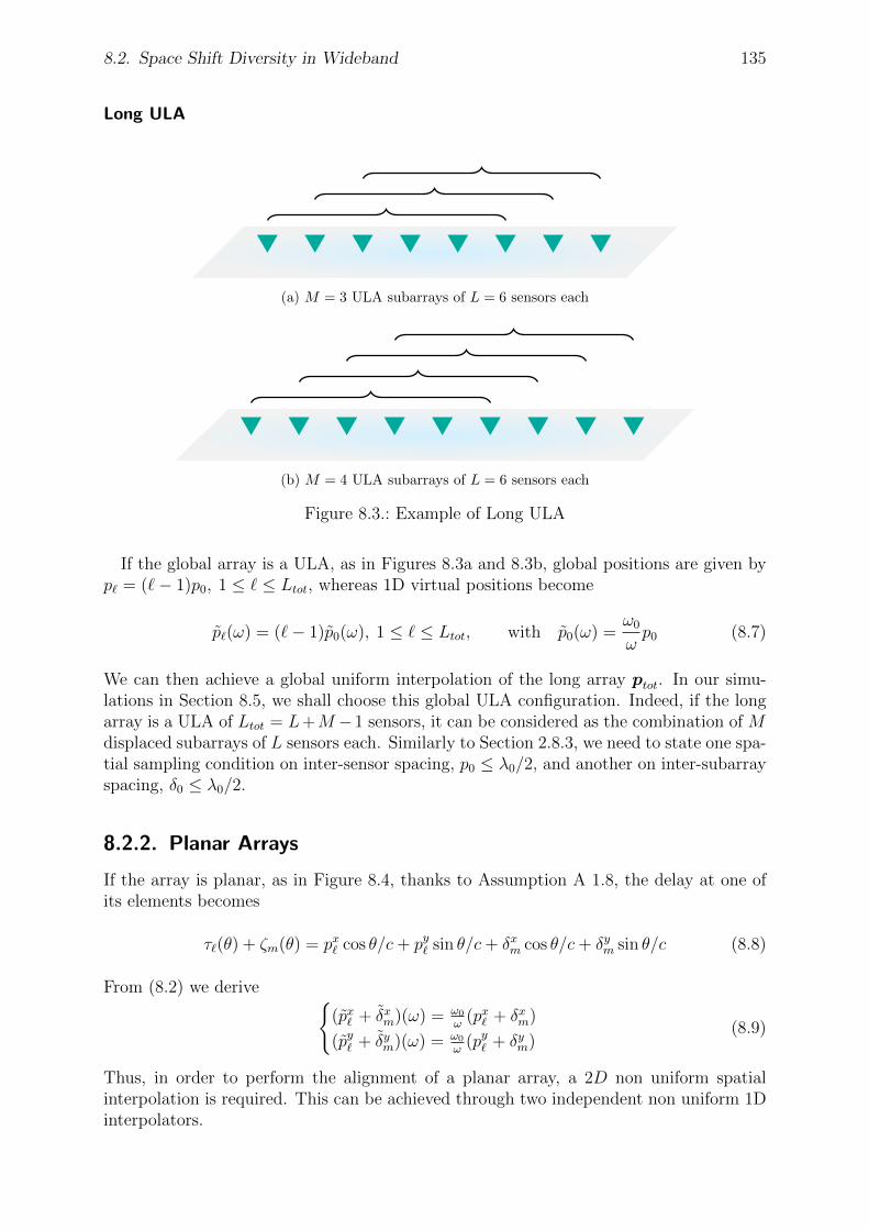
8.2. Space Shift Diversity in Wideband 135

Long ULA

(a) M = 3 ULA subarrays of L = 6 sensors each

(b) M = 4 ULA subarrays of L = 6 sensors each

Figure 8.3.: Example of Long ULA

If the global array is a ULA, as in Figures 8.3a and 8.3b, global positions are given byp` = (`− 1)p0, 1 ≤ ` ≤ Ltot, whereas 1D virtual positions become

p`(ω) = (`− 1)p0(ω), 1 ≤ ` ≤ Ltot, with p0(ω) =ω0

ωp0 (8.7)

We can then achieve a global uniform interpolation of the long array ptot. In our simu-lations in Section 8.5, we shall choose this global ULA configuration. Indeed, if the longarray is a ULA of Ltot = L+M −1 sensors, it can be considered as the combination of Mdisplaced subarrays of L sensors each. Similarly to Section 2.8.3, we need to state one spa-tial sampling condition on inter-sensor spacing, p0 ≤ λ0/2, and another on inter-subarrayspacing, δ0 ≤ λ0/2.

8.2.2. Planar Arrays

If the array is planar, as in Figure 8.4, thanks to Assumption A 1.8, the delay at one ofits elements becomes

τ`(θ) + ζm(θ) = px` cos θ/c+ py` sin θ/c+ δxm cos θ/c+ δym sin θ/c (8.8)

From (8.2) we derive (px` + δxm)(ω) = ω0

ω(px` + δxm)

(py` + δym)(ω) = ω0

ω(py` + δym)

(8.9)

Thus, in order to perform the alignment of a planar array, a 2D non uniform spatialinterpolation is required. This can be achieved through two independent non uniform 1Dinterpolators.


Figure 8.4.: Example of planar acquisition system

Long URA

If the global array is a URA , as in Figure 8.5, nominal positions are given by px` =(`x− 1)px0 , 1 ≤ `x ≤ Lxtot and py` = (`y− 1)py0, 1 ≤ `y ≤ Lytot, whereas virtual positions canbe derived independently through two uniform interpolators:

px` (ω) = (`x − 1)px0(ω), 1 ≤ `x ≤ Lxtot, with px0(ω) = ω0

ωpx0

py` (ω) = (`y − 1)py0(ω), 1 ≤ `x ≤ Lxtot, with py0(ω) = ω0

ωpy0

(8.10)

In this case, the global array of Lxtot×Lytot = (Lx +Mx−1)× (Ly +My−1) sensors canbe seen as the combination of Mx + My subarrays of Lx × Ly sensors each. Similarly toSection 2.8.3, , we need to impose two spatial sampling conditions on inter-sensor spacing:px0 ≤ λ0

2and py0 ≤ λ0

2.

px0

py0

Figure 8.5.: Example of Long URA

8.3. Polarization Diversity in Wideband 137

8.2.3. Tensor Resampling

After discretization, model (8.1) becomes

M`m(ωq) =R∑r=1

A`r(ωq)Bmr(ωq)Sqr, 1 ≤ q ≤ Q (8.11)

For each q-th frequency bin, we need to interpolate the q-th row of the mode-3 unfoldingof the data tensor X ,

X(3)q: = sq:[B(ωq)A(ωq)]T +N (3)q: ∈ C1×LM (8.12)

at positions ptot(ωq) = ptotω0

ωq. Thanks to (8.2), interpolated slices write

X(3)q: ≈ sq:[B(ω0) A(ω0)]T + N (3)q: ∈ C1×LM (8.13)

We then recompose the interpolated tensor unfolding X(3), by stacking all the interpo-

lated rows X(3)q:. This unfolding corresponds to a tensorM ≈∑R

r=1 ar(ω0)⊗ br(ω0)⊗ srM`mq ≈

∑Rr=1 A`r(ω0) Bmr(ω0)Sqr

(8.14)

We choose to study the simplest configuration of a ULA of L sensors, with M lineartranslations, as in Section 8.2.1. However, all that follows can be generalized to the planararrays through 2D spatial interpolation.

After 1D sinc spatial interpolation as described in Section 8.2.1, the factor matrices ofresulting tensor X are given by

1. A`r = exp−1

cω0p0(`− 1) cos(θr)

is the steering element of the `-th sensor.

2. Bmr = exp−1

cω0p0(m− 1) cos(θr)

is the steering element of the m-th subarray.

3. Sqr = sr(ωq) is the q-th Fourier Transform (FT) coefficient of the r-th signal.

We remind that the distance p0 between two successive sensors must be less than orequal to λ0/2, so as to avoid spatial aliasing.

8.3. Polarization Diversity in Wideband

On the other hand, we rewrite the model (6.4) for polarization diversity:

M`p(ω) =R∑r=1

A`r(ω)Kpr sr(ω), 1 ≤ p ≤ P = 3 (8.15)

where polarization vectors kr are defined in (6.5). In this case, as described in Sec-tion 6.3.5, since polarization matrix K does not depend on frequency ω, only spacematrix A(ω) needs to be interpolated at sensor positions

p`(ωq) =ω0

ωqp` (8.16)

Thus, for regular configurations, the required interpolation is simpler:


1. For a linear array of L sensors located at p`, (8.16) becomes

p`(ω) =ω0

ωp` (8.17)

Spatial resampling can then be achieved through a 1D non uniform interpolator.

2. For a ULA of L sensors located at p` = (`− 1)p0, (8.16) becomes

p`(ω) = (`− 1)p0(ω), with p0(ω) =ω0

ωp0 (8.18)

as described in Section 2.8.3. Spatial resampling can then be achieved through a1D uniform interpolator.

3. For a planar array of L sensors located at (px` , py` ), (8.16) becomes

px` (ωq) = ω0

ωqpx`

py` (ωq) = ω0

ωqpy`

(8.19)

Spatial resampling can then be achieved through two independent 1D non uniforminterpolators.

4. For a URA of Lx×Ly sensors, with nominal positions given by px` = (`x− 1)px0 andpy` = (`y − 1)py0, (8.16) becomes

px` (ω) = (`x − 1)px0(ω), with px0(ω) = ω0

ωpx0

py` (ω) = (`y − 1)py0(ω), with py0(ω) = ω0

ωpy0

(8.20)

Spatial resampling can then be achieved through two independent 1D uniform in-terpolators.

8.3.1. Tensor Resampling

After discretization, model (8.15) becomes

M`p(ωq) =R∑r=1

A`r(ωq)Kpr Sqr, 1 ≤ q ≤ Q (8.21)

For each q-th frequency bin, we need to interpolate all the P = 3 fibers of data tensor X :

x:pq = ADk(sq:)kTp: + n:pq ∈ CL, p = 1, . . . , 3 (8.22)

at positions p(ωq) = pω0

ωq, given by (8.16). Then, interpolated fibers write

x:pq = A(ω0)Dk(sq:)kTp: + n:pq ∈ CL, p = 1, . . . , 3 (8.23)

We then recompose the interpolated tensor X , by stacking all the interpolated fibersx:pq, leading to the trilinear model

M ≈∑Rr=1 ar(ω0)⊗ kr ⊗ sr

M`pq ≈∑R

r=1 A`r(ω0)Kpr Sqr, p = 1, . . . , 3(8.24)

For a ULA of L sensors, after 1D spatial interpolation of tensor fibers x:pq as described

in Section 2.8.3, the factor matrices of resulting tensor X are given by

8.4. Estimation of Signal Parameters 139

1. A`r = exp−1

cω0p0(`− 1) cos(θr)

is the steering element of the `-th sensor.

2. kr = H(θr)W (αr)w(βr) is the vector sensor response.

3. Sqr = sr(ωq) is the q-th FT coefficient of the r-th signal.

As pointed out in Section 2.8.3, the distance p0 between two successive sensors must beless than or equal to λ0/2, so as to avoid spatial aliasing.

8.4. Estimation of Signal Parameters

The factor matrices of the two Canonical Polyadic Decompositions (CPDs) in (8.14) and(8.24), A ∈ CL×R, S ∈ CQ×R, and B ∈ CM×R or K ∈ C3×R, are extracted through anALS (see Section 3.6.3 for details on tensor approximation algorithms). Initial estimatesare here given by the tensor decomposition technique [85] detailed in Section 3.5. However,unlike in Section 6.5, the noise correlation structure induced by spatial resampling is hereinnot taken into account.

Once column vectors ar, br and/or kr are extracted from ALS estimates A, B, and/orK, we can estimate DoA θr and polarization angle βr as follows.

1. DoAs θr can be estimated through a TLS algorithm1, thanks to the Vandermondestructure of the factor vector ar, as in Section 4.6.3. We refer to these estimates as

θTLSr = TLS estimate of θr as in Section 4.6.3 (8.25)

2. Polarization angle βr can be estimated through a 1D exhaustive search:

βTLSr = arg min

β‖kr − kr(θTLS

r , β)‖2 (8.26)

If there are two polarization angles, αr and βr, they can be estimated trough a 2Dexhaustive search:

(αTLSr , βTLS

r ) = arg minα,β‖kr − kr(θTLS

r , α, β)‖2 (8.27)

3. Alternatively, or as a refinement step, both DoA and polarization angles can berecovered through a joint 2D exhaustive search, as in Section 6.5.2:

θjointr = arg min

θ

∥∥∥( ar − ar(θ)br − br(θ)

)∥∥∥2

(8.28)

for space shift diversity, and

(θjointr , βjoint

r ) = arg minθ,β

∥∥∥( ar − ar(θ)kr − kr(θ, β)

)∥∥∥2

(8.29)

for polarization diversity.

However, (8.25) and (8.26), though suboptimal, have a smaller computational burden,compared to both exhaustive searches (8.28) and (8.29). Moreover, if there are twopolarization angles, αr and βr, (8.27) allows us to estimate them through a 2D search,whereas the MUSIC algorithm would need a 3D search over the parameter space (θ, α, β).Notice that the estimation of the DoA θr could be further improved using both ar andbr in (8.25).

1The TLS could also be replaced by the Structured Least Squares of [58] for further improvement.


8.5. Computer results

Experimental conditions are very similar to those of Section 6.6. We simulated R = 2white Gaussian unit-variance sources, at the sampling frequency fS = 1 kHz, during anobservation time of 64 ms and propagating at c = 1800 ms−1, which is approximately thepropagation speed of seismic S-waves through ice [117]. The number of frequency binsis Q = 17 (from fmin = 0.2 fS to fmax = 0.5 fS), whereas Spatial Nyquist condition isensured by d0 = λmin/4, where λmin = c/fmax (cf. Section 2.8.3). For every frequencybin ωq within the band [ω1, ωQ] = [2πfmin, 2πfmax], tensor interpolation of Sections 8.2.3and 8.3.1 is performed using the sinc function, as detailed in Section 8.A.

The reference frequency is chosen to be ω0 = 2πfmin, such that d(ωq) ≤ d0,∀q (i.e. thevirtual subarrays are a shrunk version of the nominal reference subarray). The estimationaccuracy of the proposed tensor method is evaluated in comparison to wideband MUSICand to the multilinear Cramer-Rao Bound (CRB), as in Chapter 6. The performancecriterion is the relative total MSE of the DoA estimates and, whenever present, of thepolarization ellipticity estimates:

MSE(θ) = 1π2

1NR

∑Nn=1


MSE(β) = 1π2

1NR

∑Nn=1


(8.30)

where θrn and βrn are the estimated DoA and ellipticity angle, respectively, of source rin the n-th MC trial, N = 2500 being the number of trials. The SNR definition below isassumed:

SNR = 10 log10

‖ X ‖2F

LMPQσ2(8.31)

8.5.1. Space Shift in Wideband

The two impinging sources arrive from the broadside: θ1 = 80 and θ2 = 100. Theacquisition system is given by a ULA of L sensors, where the following space invariancesare considered:

NB CP 3: CPD with M = 3 ULA subarrays of L − 2 sensors each: standard nar-rowband CPD (4.5) in time domain as in Chapter 4, after narrowband filtering aroundf0.

WB CP 2: WB preprocessing and CPD (8.14) with M = 2 ULA subarrays of L − 1sensors each.



The CRB, calculated as in Chapter 7, refers to the model in WB CP 3.

Notice that WB preprocessing refers to the tensor spatial interpolation described in Sec-tion 8.2, in particular in Section 8.2.1. Source DoAs where estimated using (8.25), im-plying a negligible computational complexity, compared to the exhaustive search of theMUSIC algorithm.

In particular, as for the MUSIC algorithm,

8.5. Computer results 141

WB MUSIC refers to the wideband MUSIC algorithm with covariance matrix ex-pressed in (2.51).

The label WB MUSIC SS specifies that spatial smoothing (2.62) has been performedwith M = 3.

Figures 8.6a and 8.6b show the MSE as a function of SNR, for uncorrelated and corre-lated sources, respectively, received by a ULA of L = 20 sensors.

Figures 8.7a and 8.7b show the MSE as a function of the angular separation betweenR = 2 sources, for uncorrelated and correlated sources, respectively, received by a ULAof L = 20 sensors. In this case, DoAs are given by θ1 = 90−∆θ/2 and θ2 = 90+ ∆θ/2.

Similarly, Figures 8.8a and 8.8b show the MSE as a function of the number of sensors,L, for uncorrelated and correlated sources, respectively, at a SNR of 20 dB.

The tensor decomposition with M ∈ 3, 4 space shifts yields better results when thenumber of sensors or the SNR increase. The WB preprocessing significantly improvesthe performance of the narrowband tensor estimation, NB CP 3. Moreover, tensor-basedwideband DoA estimation appears to outperform the wideband MUSIC algorithm, in thepresent experimental conditions.

In Figures 8.6b and especially 8.6a at high SNR, we notice a saturation of the MSE,due to the interpolation error, resulting in a progressively significant gap from the CRB.

A slight saturation or deterioration of the performance of the DoA algorithms takesplace when the two sources move away from the broadside (θr ≈ 0), as demonstrated inFigures 8.7a and 8.7b.


0 10 20 30 4010−10

10−9

10−8

10−7

10−6

10−5

10−4

10−3

10−2

10−1

100

SNR [dB]

MSE

[rad

2 ]NB CP 3WB CP 2WB CP 3WB CP 4WB MUSICWB MUSIC SSCRB

(a) DoA estimation - Uncorrelated sources, L = 20 sensors

0 10 20 30 4010−10

10−9

10−8

10−7

10−6

10−5

10−4

10−3

10−2

10−1

100

SNR [dB]

MSE

[rad

2 ]

NB CP 3WB CP 2WB CP 3WB CP 4WB MUSICWB MUSIC SSCRB

(b) DoA estimation - Correlated sources: ρ = 0.9, L = 20 sensors

Figure 8.6.: MSE vs SNR - space shift diversity


5 10 15 25 40 55 70 9010−8

10−7

10−6

10−5

10−4

10−3

10−2

Angular separation [deg]

MSE

[rad


(a) DoA estimation - Uncorrelated sources, L = 20 sensors

5 10 15 25 40 55 70 9010−8

10−7

10−6

10−5

10−4

10−3

10−2

10−1

100


MSE

[rad

2 ]


(b) DoA estimation - Correlated sources: ρ = 0.9, L = 20 sensors

Figure 8.7.: MSE vs angular separation - space shift diversity


6 10 15 20 30

10−8

10−7

10−6

10−5

10−4

10−3

10−2

10−1

L (number of sensors)

MSE

[rad


(a) DoA estimation - Uncorrelated sources, SNR = 20 dB

6 10 15 20 30

10−8

10−7

10−6

10−5

10−4

10−3

10−2

10−1

L (number of sensors)

MSE

[rad

2 ]


(b) DoA estimation - Correlated sources: ρ = 0.9, SNR = 20 dB

Figure 8.8.: MSE vs L - space shift diversity


8.5.2. Polarization in Wideband

We now replace space shift diversity of Section 8.5.1 with polarization diversity, as inSection 8.3. The two impinging sources are Rayleigh waves, i.e. α = 0, ψ = 0 (coplanarwith the array), arriving from the broadside: θ1 = 80 and θ2 = 100, and differentlypolarized: β1 = −20 and β2 = 10. This configuration is similar to that of Section 6.6.2.The acquisition system is given by a ULA of L = 20 sensors, with P = 3 polarizationcomponents. Hereafter, we compare the following methods:

NB CP TLS: standard narrowband CPD (5.27) in time domain as in Section 5.3,after narrowband filtering around f0. Signal parameters are estimated using (8.25) and(8.26).

WB CP TLS: WB preprocessing is applied and, after CPD (8.24), signal parametersare estimated using (8.25) and (8.26).

WB CP Joint: WB preprocessing is applied and, after CPD (8.24), signal parametersare estimated using (8.29).

WB Scalar MUSIC, via an incoherent average of P covariances.

WB Vector MUSIC in Section 5.3.1, where the array manifold takes into accountwave polarization parameters, via a coherently averaged covariance matrix of size PL×PL.

Notice that WB preprocessing refers to the spatial interpolation described in Section 8.3.

Figures 8.9a and 8.9b show the MSE as a function of SNR, for DoA and polarization es-timation, respectively. As for space shift diversity in Section 8.5.1, the proposed widebandtensor method significantly improve its narrowband counterpart, and outperform the WBVector MUSIC algorithm, as for both DoA and polarization estimation. We notice thatWB CP Joint is slightly better than WB CP TLS, as it achieves a joint estimation fromfactor matrices A and K.

However, the advantage of WB CP TLS lies in its lightest computational cost, as aTLS followed by a 1D search are less demanding than a 2D search. Finally, in Figure8.9a we can observe an estimation bias of the DoA estimates of all the wideband methodsfor high SNR, due to the interpolation error. A similar bias also affects the WB MUSICpolarization estimation in Figure 8.9b.


0 10 20 30 4010−12

10−11

10−10

10−9

10−8

10−7

10−6

10−5

10−4

10−3

10−2

SNR [dB]

MSE

[rad

2 ]

NB CPWB CP TLSWB CP JointWB Vector MUSICWB Scalar MUSICCRB

(a) DoA estimation - Uncorrelated sources - L = 20 sensors

0 10 20 30 4010−8

10−7

10−6

10−5

10−4

10−3

10−2

SNR [dB]

MSE

[rad

2 ]

NB CPWB CP TLSWB CP JointWB Vector MUSICCRB

(b) Polarization estimation - Uncorrelated sources - L = 20 sensors

Figure 8.9.: MSE vs SNR - polarization diversity

8.6. Conclusions and Perspectives 147

8.6. Conclusions and Perspectives

Space and frequency smoothing have been realized in a deterministic framework, and weshowed that polarization can replace space shift diversity in the tensor formulation, as inChapter 6.

In this chapter, we extended the spatial interpolation technique of Section 2.8.3 towideband tensor-based algorithms. This development can be seen as an alternative tothe multilinear interpolation of Chapter 6, whenever the acquisition system has a regularstructure, such as the ULA structure. In this case, the division into angular sectors is nolonger necessary.

However, we studied so far only the ULA configuration, as spatial interpolation is easierto handle. The interest of the ULA configuration is also related to the large numberof applications that resort to such arrays. For instance, in multidimensional harmonicretrieval, data tensors have a Vandermonde structure in multiple dimensions. In thiscase, multiple interpolations can be applied independently, as a generalization of (8.6)and (8.10). This was the object of [163], who extended our idea in [119] to MIMO radars,through multiple subsequent linear interpolations. In particular, [163] showed that linearinterpolation performed better for their purpose, compared to the sinc interpolation.

Similarly, as a perspective, the results in the last two chapters could be extended to thedesign of wideband preprocessing routines for 2D ESRPIT [164] and DD ESPRIT [60],as well as for multidimensional harmonic retrieval [61], as in [163].

The wideband tensor estimation through spatial resampling could also be improved ifthe noise covariance structure induced by interpolation were taken into account withinthe tensor CPD approximation, as in Section 6.5.

In the end of next chapter, the proposed method is applied to real seismic data recordedby a ULA for DoA estimation.

Appendix

8.A. Array 1D Interpolation

8.A.1. Sinc Interpolation

Interpolation is related to signal resampling as follows:

1. Thanks to the Shannon sampling theorem [100], the continuous signal x(t) can bereconstructed from its samples x(nTs):

x(t) =+∞∑

k=−∞

x(kTs) g(t− kTs) (8.32)

2. Only once the interpolating process has been expressed, the signal can be resampledat a new rate T ′s as follows:

x(t)|t=nT ′s =+∞∑

k=−∞

x(kTs) g(nT ′s − kTs) (8.33)

The most common interpolating function is generally the sinc function:

g(t− kTs) = sinc

(t− kTsTs

)(8.34)

leading to

x(t) =

[+∞∑

k=−∞

x(kTs)δ(t− kTs)]∗ sinc

(t

T

)(8.35)

Since in practice only a finite number of samples is available, it is advisable to truncatethe sinc function with a window of length ∆T enhancing the central samples and relatedto the signal frequency behavior. This action is named apodization. As for our implemen-tation, we chose a rectangular window W with a support of ∆T = 5 time samples:

sincW (t) =sin(πtf)

πtf1W (t) (8.36)

where 1W (t) is the indicator function of the window W . The parameter f that we fixedto 0.4 controls the smoothness of the sinc interpolation.

8.A.2. Spatial Interpolation

Analogously, we define a spatial interpolator to reconstruct the signal at frequency ωq atany point p in space, x(ωq, p), from its samples at nominal sensor positions p` = `p0:

x(ωq, p) =+∞∑`=−∞

x(ωq, kp0) g(p− kp0) (8.37)

9. Tensor Decomposition of SeismicVolume Waves

9.1. Contribution

In this chapter, we consider the problem of DoA estimation of seismic plane waves imping-ing on an array of sensors from a new deterministic perspective using tensor decompositiontechniques. In addition to temporal and spatial sampling of Chapter 1, we take into ac-count further information, based on the different propagation speeds of body waves (Pand S) through solid media. We evaluate performance through simulated data in termsof the Cramer-Rao Bound (CRB) and in comparison with other reference methods suchas ESPRIT and MUSIC, in the presence of additive Gaussian circular noise (Assump-tion A 1.12). We then apply the proposed approach to real seismic data recorded at theArgentiere glacier, occurring at the interface between the ice mass and the underlyingbedrock. Information about propagation speed diversity is not taken into account byexisting models in array processing. The discovered advantage in terms of the averageerror in estimating the direction of arrival of body waves is noteworthy, especially for alow number of sensors, and in separating closely located sources. Additionally, we observean improvement of precision in processing real seismic data.

Our work was published in the journal article [117], and was source of inspiration for themore general development of the wideband tensor DoA estimation described in Chapter 6and Chapter 8. Our work was cited by a review article on cryoseismology [111] and by ajournal article on non-negative tensor decompositions for large datasets [154].

9.2. Context

In the context of seismic monitoring, seismology aims at studying waves generated byrupture phenomena taking place within a volume of interest (rock, ice, etc.). Althoughthe most interesting events take place at a certain depth - mostly unknown - within theanalyzed volume, acquisition systems and sensor arrays are most often located close tothe surface. The main quantity to be measured is ground displacement (in the form ofits derivative - velocity - or its second derivative - acceleration), produced by impingingelastic waves. The localization of the sources forms the first requirement of data analysis,in order to prevent damage provoked by seismic events, and to monitor the activity ofcomplex structures such as glaciers or volcanoes. Seismic arrays, after being introducedin the 1960s, have made essential contributions to this problem. These arrays consist ofnumerous seismometers placed at discrete points in space in a well-defined configuration[123]: apart from an improvement of SNR by combining individual sensor recordings, theyhave been used to refine models of the Earth’s interior, through classical tools such asbeamforming, slant stacking techniques and frequency-wave number analysis.

150 9. Tensor Decomposition of Seismic Volume Waves

This chapter exploits another type of diversity, in addition to spatial and temporalsampling traditionally employed in array processing (cf. Section 5.2 for a detailed ex-planation of the concept of diversity): the propagation speed diversity1 of body wavesthrough solids, namely pressure (P) and shear (S) waves. Current array processing meth-ods like [131, 126] only focus on information conveyed by a single body wave, like theP wave, whereas the contents delivered by the other is somehow wasted. Our approachintends to exploit this information as a whole, whereas translational invariance used in[136] and detailed in Chapter 4 is no longer necessary.

This chapter is organized as follows. Section 9.3 presents the physical model and someassumptions. Our tensor deterministic method for DoA estimation, exploiting the propa-gation speed diversity of body waves, is presented in Section 9.4. Simulated data and realseismic data are treated in Sections 9.5 and 9.6 respectively. Computer results in SectionsSection 9.5 are compared with 2D subspace methods of Chapter 2 and with the CRB ofChapter 7. An application to icequakes recorded at the Argentiere glacier in 2012 is theobject of Section 9.7.

9.3. Physical model and assumptions

When one wants to estimate and localize seismic events originating at depth, one has todeal with a double arrival of elastic body waves: P waves and S waves, which are detailedin Section 1.6. For the physical model of wave propagation, the following properties areassumed, in addition to all the assumptions of Sections 1.2.2 and 1.6:

A 9.1. The impulse responses of particle motion is the only source of variability betweenimpinging P and S waves.

and in order to allow the multilinearity and separability of the final model:

A 9.2. We filter P and S signals in a narrow-band around f1 = ω1/2π and f2 = ω2/2π,respectively, such that v1

f1= v2

f2= λ is constant, where λ refers to the wavelength of

impinging waves.

A 9.3. Base-band P and S signals propagating from the same source event and receivedin two different narrow bands around f1 and f2 are proportional:

w2bf (t) = α(f1, f2) w

1bf (t) (9.1)

See (9.38) in Section 9.A for more details.

Furthermore, we state the following notation, which will be subsequently used:

A 9.4. In order to avoid scale indeterminacies in tensor decomposition, the P wave w1bf (t)

is fixed up to a scale factor (see Section 9.A for more details).

1Since the focus is on narrow-band processing, the distinction between group and phase propagationvelocities is irrelevant.

9.4. Speed diversity in tensor format 151

9.4. Speed diversity in tensor format

The advantage of the tensor formalism lies in its ability to restore the identifiability of sig-nal parameters: impinging sources, their directions of arrival, and the related connectionbetween P and S waves.

Propagation speed diversity may be seen as equivalent to a frequency diversity betweenP and S waves, under Assumption A 1.3 and properties A 1.21, A 9.2 and A 9.3. Theproposed model for propagation speed diversity will be subsequently developed on thebasis of the linear relation below:

g(t, f) =R∑r=1

wr(t) αr(f) ⇐⇒ Gtk =R∑r=1

Sr[t] Cr(fk) (9.2)

where the latter equation represents the discretization of the former. fk denotes theworking frequency for P and S waves (k = 1 for the P wave and k = 2 for the S wave), asdefined in A 9.2; it is chosen by the user as a function of propagation speed vk; αr(·) is acomplex unknown coefficient.

The focus of our work consists in integrating at the same time the spatial, temporaland speed diversities, respectively embodied by matrices A ∈ CL×R, S ∈ CT×R andC ∈ C2×R.

P and S waves are generated by the same physical source but propagate at two differ-ent velocities, v1 and v2 respectively, and correspond to different propagation modalities(compression and share waves respectively). Thus, P and S signals received at position pand at time t are respectively given by

yP (p, t) =∑R

r=1wPr (t− τPr (p)) + nP (t,p)

yS(p, t) =∑R

r=1wSr (t− τSr (p)) + nS(t,p)

(9.3)

where τPr , τSr express the respective delays for P and S signals recorded at positionp. The signal received at a point p in space contains R sources of interest plus anadditive noise: under assumptions A 1.1 and A 1.3, the time delays of P and S wavescorrespond to the phase shifts exp

−$P

r (p)

and exp−$S

r (p)

respectively, with$Pr (p) = ω1

v1pTd(θr), $

Sr (p) = ω2

v2pTd(θr).

With properties A 9.2, A 9.3 and A 9.4, records produced by the r-th source containtwo delayed narrowband waves propagating at frequencies f1, f2 at velocities v1 and v2,yielding two resulting waves with the same wavelength λ. After windowing, filtering andaligning the two waves (cf Section 9.6 for details), we can model them as a separablefunction of 3 variables:

x(p, t, f) =R∑r=1

exp −$r(p) wr(t)αr(f) + n(p, t, f) (9.4)

where coefficient αr(f) is the same as in (9.2) and $r(p) = 2πλpTd(θr). Thus, in the

absence of noise n(p, t, f), function x(p, t, f) decomposes into a sum of R functions whosevariables separate. Discretization of (9.4) corresponds to a 3-way array of finite dimensionsL×T × 2 (L sensors located at p`, T time samples and K = 2 propagation velocities vk):

X`tk =R∑r=1

exp −$r(p`) wr(t) αr(fk) +N`tk (9.5)


where frequency fk, k = 1, 2 is fixed according to property A 9.2(λ = v1

f1= v2

f2

). Notice

that, thanks to convention A 9.4, the complex envelopes of the P and S waves are expressedin (9.5) as

w1bf (t) = w(t) P wave complex envelope

w2bf (t) = α(f2) w(t) S wave complex envelope

(9.6)

Thus, the tensor Canonical Polyadic Decomposition (CPD) model X = M+N is theresult of stacking the two matrix slices M ::1 and M ::2, corresponding to P and S wavesrespectively, as in Figure 9.1:

S wave

P wave

space

timepropagationspeed

Figure 9.1.: P and S slices, M ::1 and M ::2

X =

∑Rr=1 ar ⊗ sr ⊗ cr + N

X`tk =∑R

r A`r Str Ckr +N`tk

(9.7)

where rank-R corresponds to the number of sources, supposed known, thanks to Assump-tion A 1.10, and N refers to additive noise. The physical meaning of the three factormatrices is as follows:


Str = wr(t) refers to time diversity

Ckr = αr(fk) refers to speed diversity

(9.8)

where τ`(θr) = pT` d(θr)/c refers to the time delay at sensor ` w.r.t. the reference sensor.

Therefore, as in Section 4.3.1, we fix 2R parameters without restricting the generality.More precisely, based on properties described in Section 9.3, we assume the following:

1. From property A 4.2 we refer to the first sensor by index 1, with p1 = 0:

A1r = exp−$1r = exp

−2π

λpT1d(θr)

= 1 ∀r (9.9)

9.4. Speed diversity in tensor format 153

2. From property A 9.3 we refer to the P wave by index 1:

αr(f1) = 1, ∀r =⇒ C1r = 1, ∀r (9.10)

Thus, we impose the first rows of matrices A and C to be formed of ones. Then wepull column-wise the remaining scaling coefficients, ςr A1r C1r, into matrix S. Moreprecisely, we fix all scale indeterminacies through the following transformation:

(ar, sr, cr, ςr)←−(arA1r

, ςr A1r C1r sr,crC1r

, 1

)(9.11)


In the present chapter, we deal with simpler examples when R = 1 as for glacier data(Section 9.6) and R = 2 relative to simulated data (cf. Section 9.5), so that essentialuniqueness of a decomposition is always guaranteed (see Section 3.3.5 for details).

9.4.1. Estimation of Signal Parameters


x = vecX =R∑r=1

cr sr ar + n (9.12)

where denotes the Kronecker product, as defined in [26, 75] (cf. (3.22) for generictensor order D). Since, thanks to Assumption A 1.11, the measurement noise vector,n = vecN , is circular white Gaussian and isotropic, i.e. with zero mean and covarianceΣ = σ2I, the log-likelihood takes the form:


where µ =∑R

r=1 cr sr ar is unknown and constrained by its parameterization ϑ =[θ, vecS, vecC]. For the CRB of the tensor DoA estimation, see Chapter 7.

Although the optimal solution is given by the global maximum of Υ(ϑ), we proposea suboptimal two-step procedure in the same spirit as [128], with smaller computationalburden: first Υ is maximized with respect to parameter ξ = [vecA, vecS, vecC]through the decomposition algorithm of [85] detailed in Section 3.5; then DoAs and theother signal parameters can be estimated as follows.

1. Direction of arrival θr of the r-th source impinging on the array is calculated fromA`r = exp

−2π

λpT` d(θr)

as in Section 4.6, and, for ULAs, in Section 4.6.3.

2. The signal sr(t) of the r-th source is extracted up to a scaling factor directly frommatrix S, as in Section 4.7.

wr(t) ∝ Str, t = 1, ..., T (9.14)

3. The complex multiplicative coefficient αr(fk) is extracted directly from matrix C:

αr(fk) = Ckr (9.15)


9.5. Numerical simulations

Signals were simulated according to sampling conditions, that are typically those selectedfor experiments at Argentiere (cf. [63, 64]) and emulate the normal seismic activity ofa glacier. Estimation efficiency was evaluated in comparison with two other narrowbandalgorithms, ESPRIT [126] and MUSIC [131, 140], and with deterministic CRB as abenchmark. In the following figures, CRB-2D indicates the CRB of the MUSIC algorithm[140], whereas CRB-3D indicates the CRB of the tensor CPD.

The performance criterion is the Root Mean Square Error (RMSE) on the DoA:

RMSE(θ) =

√√√√ 1

NR

N∑n=1

R∑r=1

(θrn − θr)2, (9.16)

where θrn is the estimated DoA of source r in the n-th MC trial, N being the number oftrials. The number of simultaneous sources was chosen to be R = 2. The SNR definitionfor P wave was:

SNR = 10 log10

‖ µP ‖2

LTσ2n

(9.17)

where µP = vecM ::1 refers to the P wave. This is consistent with previous works, wherethe S wave data is traditionally thrown away even if received. In fact, in our simulationswe applied MUSIC and ESPRIT on the P wave only.

We have the following values:

1. We use values for P and S wave velocities through ice, as in [63, 150]: v1 = 3600 m s−1

and v2 = 1610 m s−1.

2. v1v2

= f1f2≈ 2.24.

3. f1 = 193 Hz, f2 = 86 Hz.

4. Time duration of simulated records: 201 ms.

5. Configuration of the array: ULA with inter-sensor distance p0 = 10 m. Three arrayswere simulated, each with a different number of sensors: L ∈ 3, 10, 30.

6. Simulated directions of arrivals:Figure 1: endfire θ1 = 30, θ2 = 50

Figure 2: broadside θ1 = 80, θ2 = 100

Figure 3a: endfire θ1 = 45 −∆θ/2, θ2 = 45 + ∆θ/2

Figure 3b: broadside θ1 = 90 −∆θ/2, θ2 = 90 + ∆θ/2

(9.18)

where ∆θ refers to the x-axis of Figure 9.5 (the overall angular separation between the

two sources).

A simple source was simulated as approximately narrowband: a signal carried by asinusoid modulated by a Kaiser window of envelope ar(t):

skr(t) = akr(t) expφkr(t) expωkt (9.19)

9.5. Numerical simulations 155

where φkr(t) are independently drawn in [0, 2π) for every t. Since narrowband ωk isknown for P and S waves, simulated signal skr(t) is brought to the baseband throughdemodulation:

skr(t) = akr(t) expφkr(t) (9.20)

MC simulations (N = 200 trials) show a superior performance of the CPD with respectto MUSIC and ESPRIT algorithms, in the sense of the RMSE defined in (8.30), especiallyfor a low number of sensors composing the array. For larger number of sensors, theperformance of MUSIC and CPD becomes comparable. In particular, Figures 9.2 and9.3 illustrate computer simulations for a variable number of sensors, L ∈ 3, 10, 30,composing the array and for different configurations of sources impinging from a broadside(perpendicular to the array) or endfire (laterally to the array) perspective.

The following observations can be made.

• For low SNR values, the RMSE does not increase anymore at some point, as SNRdecreases. This can be observed in particular for L = 3 in Figures 9.2a and 9.3a.This is a known saturation phenomenon [151], which is due to the fact that estimatedangles are bounded. For such low values of SNR, the CRB becomes meaningless.

• For larger numbers of sensors, e.g. L = 10 or L = 30, the latter saturation phe-nomenon is not yet observed at SNR = 5 dB, and one can observe a take-off of theRMSEs from their CRBs. This threshold effect is well known and expected at lowSNR values [15].

• The performance of CPD and ESPRIT methods does not reach the CRB for L = 10or L = 30. This loss can be explained by the 2-step nature of the estimation process,which consists of estimating first steering vectors, and then corresponding DoAs ina second stage (cf. Section 4.6).

• For L = 10 and L = 30, MUSIC seems to perform better than ESPRIT. This is dueto the fact that MUSIC finds the DoA by executing an exhaustive search, which ishence a one-stage procedure.

Figures 9.4 and 9.5 represent the evolution of the RMSE (obtained with N = 300trials) with respect to the angular separation of the two simultaneous sources, for a fixedSNR of 20 dB: the tendency is an evident predominance in the performance of the CPDalgorithm, especially for closely spaced sources.

To conclude, the advantage of CPD over ESPRIT is always present, whereas CPDoutperforms MUSIC substantially when the number of sensors remains limited or whensources are close to each other (less than 15 degrees).


0 10 20 30 40 5010−3

10−2

10−1

100

101

SNR [dB]

RM

SE[r

ad]

CPDMUSICESPRITCRB-3DCRB-2D

(a) array of L = 3 sensors

0 10 20 30 40 5010−5

10−4

10−3

10−2

10−1

100

101

SNR [dB]

RM

SE[r

ad]


(b) array of L = 10 sensors

0 10 20 30 40 5010−5

10−4

10−3

10−2

10−1

100

SNR [dB]

RM

SE[r

ad]


(c) array of L = 30 sensors

Figure 9.2.: DoA RMSE [rad] vs SNR [dB] for various numbers of sensors and T = 20time samples. Broadside perspective: DoAs = [80, 100].

9.5. Numerical simulations 157

0 10 20 30 40 5010−3

10−2

10−1

100

101

SNR [dB]

RM

SE[r

ad]


(a) Array of L = 3 sensors

0 10 20 30 40 5010−4

10−3

10−2

10−1

100

101

SNR [dB]

RM

SE[r

ad]


(b) Array of L = 10 sensors

0 10 20 30 40 5010−5

10−4

10−3

10−2

10−1

100

101

SNR [dB]

RM

SE[r

ad]


(c) Array of L = 30 sensors

Figure 9.3.: DoA RMSE [rad] vs SNR [dB] for various numbers of sensors and T = 20time samples. Endfire perspective: DoAs = [30, 50].


0 10 20 30 40 50 60 7010−3

10−2

10−1

100


RM

SE[r

ad]

CPDMUSICESPRIT

Figure 9.4.: RMSE [rad] vs angular separation [deg] - broadside perspective

0 10 20 30 40 50 60 7010−3

10−2

10−1

100

101


RM

SE[r

ad]

CPDMUSICESPRIT

Figure 9.5.: RMSE [rad] vs angular separation [deg] - endfire perspective

9.6. Application to Real Seismic Data 159

9.6. Application to Real Seismic Data

We propose a procedure for real seismic data, according to the following order:

1. Detection of an event.

2. Windowing of P and S waves.

3. Alignment of P and S waves.

4. Choice of working frequencies f1 and f2, satisfying assumption A 9.2 and respectingthe signal spectral content.

5. Narrowband filtering of P waves around f1 and of S waves around f2.

6. Constitution of the data tensor X from the two slicesX ::1 = XP andX ::2 = XS.

7. Tensor decomposition of X , according to CPD model in (9.7).

Points 1) – 5) constitute a preprocessing stage. Points 6) – 7) are at the core of the tensorapproach proposed in Section 9.4. In the present section, we detail some preprocessingsteps: windowing, alignment, choice of the working frequencies and filtering.

9.6.1. Windowing and Alignment

Since recorded P and S waves are usually consecutive and distinct in time, they need tobe selected and cropped, so as to form two T × L slices, where T is the number of timesamples, and L the number of sensors: X ::1 and X ::2. The additive model consists in adeterministic component and random noise:

xP(t− tP` ) = wP (t− tP` ) + n`(t− tP` )

xS(t− tS` + ξPS) = wS(t− tS` + ξPS) + n`(t− tS` + ξPS)(9.21)

where ` = 1, ..., L, and ξPS is the alignment error between P and S slices. The narrowbandapproximation A 1.3 at a given ostensible wavelength λ = v1

f1= v2

f2gives

xP(t− tP` ) ' αP w(t) exp−$`+ n`(t− tP` )

xS(t− tS` + ξPS) ' αS w(t+ ξPS) exp−$`+ n`(t− tS` + ξPS)(9.22)

where $` = 2πλpT` d(θ), and coefficients αP and αS directly derive from property A 9.3.

Alignment is pursued through cross-correlation between P and S narrowband complexenvelopes after the detection process, which is theoretically justified provided signals arejointly stationary and uncorrelated to noise n`(t) (Assumption A 1.14):

RPS` (τ, ξPS) = RPS

` (τ + ξPS) =

= ExP(t− tP` ) xS(t− tS` + τ + ξPS) =

= αP αS exp−2$`Rww(τ + ξPS)

(9.23)

where Rww(τ + ξPS) = Ew(t)w∗(t+ τ + ξPS).If the alignment is fulfilled on the reference sensor (` = 1), we seek to maximize

RPS1 (τ + ξPS) = αP αS R

ww(τ + ξPS) (9.24)

which attains its maximum for τmax = −ξPS. Once τmax is determined, P and S wavescan be aligned.


9.6.2. Working Frequencies and Filtering

In order to maintain a constant wavelength λ, which is necessary for the separability of themultilinear model in (9.7), a compromise needs to be reached in extracting the dominantfrequencies, so as to match the ideal condition λ = v1

f1= v2

f2in property A 9.2. Within

the set of four parameters determining the wavelength λ, v1, v2, f1, f2, one only needs 3degrees of freedom to determine optimal working conditions. P and S wave propagationvelocities v1 and v2 are given by geophysical active analysis of known waves reflecting fromthe surface to the glacier bed [63], [156]. The only parameter subject to optimization isthen P or S wave frequency f1 or f2. If f1 is chosen as the free parameter and optimized,then f2 directly derives from property A 9.2

f2 =v2

v1

f1 =v2

λ(9.25)

The optimization for f1 is fulfilled by minimizing the square norm of the CPD tensordecomposition error:

f1 = arg minf1

∣∣∣∣∣∣∣∣x(f1) −R∑r=1

ςr a(f1)r s(f1)

r c(f1)r

∣∣∣∣∣∣∣∣2 (9.26)

where x(f1) = vecX (f1) refers to the data array after narrowband filtering aroundf1 ∈ (0, fS/2), given sampling frequency fS; see (3.46) for the definition of tensor approx-imation. Then, from Equation (9.25), we have f2 = v2

v1f1.

Recorded P and S waves have to be filtered around f1 and f2 respectively, in order tosatisfy the narrowband assumption A 1.3. Moreover, a tradeoff has to be sought withrespect to the signal spectral content, in case the ratio of the dominant frequencies doesnot reflect the ratio of the velocities of P and S waves, according to property A 9.2.

9.7. Application to the Argentiere Glacier

The Argentiere glacier is a 10 km long glacier located in the French side of the Mont Blancmassif, covering a 19 km2 surface (see pictures in Figure 9.6).

Figure 9.6.: Pictures of the Argentiere glacier

9.7. Application to the Argentiere Glacier 161

It is characterized by high seismic activity, as stated in [124, 125]. Temperate Alpineglaciers are characterized by ice remaining at melting point, deformed by two main mech-anisms: plastic deformation of ice and basal sliding. The underneath flow of water playsan important role in basal sliding, because it modifies the water pressure. Furthermore,brittle behavior of ice is the reason of the sudden openings of crevasses and falls of seracson the surface of a glacier, with indirect effects on glacial hydrology by means of watertransfer from the surface to greater depth zones.

An array composed of 9 velocimeters (model is Sismob IHR1C in Figure 9.7, 1 com-ponent, 2 Hz eigenfrequency, 1 kHz sampling frequency) pointing in the direction perpen-dicular to the glacier motion was placed on the glacier surface at 2400 m above sea level(see Figure 9.8).

Figure 9.7.: Pictures of the geophone used for our experiment

Figure 9.8.: Glacier structure and experimental set


The sensors within the array were spaced out at 10 m intervals, and the thickness ofthe glacier under the array is about 190 m [63, 155]. Deep events of interest took place at450 m from the array, at a depth of about 190 m from the surface [63]. The general caseinvolves R far field sources impinging on the array, at a large unknown distance [63], inthe presence of noise, thus allowing us to use the plane wave approximation A 1.1.

Real data from the glacier are processed via speed diversity in Section 9.7.1, repeti-tion diversity in Section 9.7.2, and through the proposed wideband tensor approach inSection 9.7.3.

9.7.1. Speed Diversity - Narrowband

The tensor DoA estimation via speed diversity proposed in Section 9.4 was applied tothe 27 deep events recorded by the array during November 2012. These events wereassociated with the same cluster of deep events [63], on the basis of their waveformsimilarities, through cross-correlation. We use values for P and S wave velocities throughice, as in [150, 63]: v1 = 3600 m s−1 and v2 = 1610 m s−1, according to Property A 1.21.An example of one deep event recorded by the 9 sensors with distinct P and S waves isprovided in Figure 9.9.

The frequency optimization (i.e. the choice of the working frequencies f1 and f2) wasachieved throughout the dataset from the same cluster of events, after preprocessing ofrecorded signals (see Section 9.6.2 for details). Results are shown in Figure 9.10.

The median dominant frequency f1 of the P wave was then calculated. Thus, all theP waves from the cluster are filtered around f1 = 229 Hz, whereas all the S waves arefiltered around f2 = v2

v1f1 = 102 Hz. Then, tensor CPD estimation in Section 9.4.1 was

applied. The narrowband filter bandwidth was BW = 0.015fs. The derivation of f1 andf2 is coherent with the spectral content of P and S waves, as shown in Figure 9.13.

Beside filtering, we did not deconvolve the signals from any instrument response, be-cause the frequency content of the icequakes is much higher than the resonance frequencyof the velocimeters (2 Hz). We thus consider that the instrument response is flat.

DoA estimation is performed over the dataset with the following methods:

MUSIC over P and S waves separately.

ESPRIT over P and S waves separately.

CP PS: joint tensor CPD with speed diversity.

Results are shown in Figure 9.11: the dispersion of the DoA estimates through thejoint CPD of P and S waves (CP PS) is smaller than that of MUSIC and ESPRIT forP and S waves separately. ESPRIT yields better results than MUSIC, perhaps becauseit is more robust to array imperfections, as stated in Section 2.6.2. However, ESPRITrequires two identical subarrays deducible from each other via a translation, whereas theproposed tensor method has no such requirement.


0 20 40 60 80 100 120 140 160 180 200 220 240 260−1,000−500

0500

1,0000 20 40 60 80 100 120 140 160 180 200 220 240 260

−2,000−1,500−1,000−500

0

0 20 40 60 80 100 120 140 160 180 200 220 240 260−2,000−1,000

01,0002,000

0 20 40 60 80 100 120 140 160 180 200 220 240 260−4,000−3,000−2,000−1,000

0

0 20 40 60 80 100 120 140 160 180 200 220 240 260−4,000−2,0000

2,0004,000

0 20 40 60 80 100 120 140 160 180 200 220 240 260−2,000−1,000

01,0002,000

0 20 40 60 80 100 120 140 160 180 200 220 240 260−4,000−3,000−2,000−1,000

0

0 20 40 60 80 100 120 140 160 180 200 220 240 2600

1,0002,0003,0004,000

0 20 40 60 80 100 120 140 160 180 200 220 240 260−4,000−3,000−2,000−1,000

0

time [ms]

Figure 9.9.: Example of an event at the Argentiere glacier - November 2012Record from the array with distinct P and S waves - vertical component


0 2 4 6 8 10 12 14 16 18 20 22 24 26 28 300

50

100

150

200

250

300

350

400

450

500

Event cardinality within the cluster

Freq

ueny

[Hz]

Figure 9.10.: Optimized working frequency for P wave, f1

40

50

60

70

80

90

100

110

120

130

140

150

160

CP PS MUSIC P MUSIC S ESPRIT P ESPRIT S

Est

imat

edD

oA[d

eg]

Figure 9.11.: DoA estimation throughout the cluster of deep events - propagation speed


9.7.2. Repetition Diversity

Since we deal with multiple events from the same seismic cluster in the depths of theglacier, we can also make use of repetition diversity, as explained in (5.8). Notice thatafter detection all the events have been previously centered around zero, divided by theirstandard deviation, and aligned through cross-correlation (see Figure 9.12 for receivedsignals and Figure 9.13 for the estimate of their power spectral density).

0 10 20 30 40 50 60−5

−4

−3

−2

−1

0

1

2

3

4

5

time [ms]

sens

orou

tput

(a) P waves

0 10 20 30 40 50 60−4

−3

−2

−1

0

1

2

3

4

time [ms]

sens

orou

tput

(b) S waves

Figure 9.12.: P and S waves from the same seismic cluster - sensor ` = 6


0 50 100 150 200 250 300 350 400 450 5000

0.1

0.2

0.3

0.4

0.5

0.6

0.7

0.8

0.9

frequency [Hz]

Wel

chpe

riod

ogra

m

(a) P waves

0 50 100 150 200 250 300 350 400 450 5000

0.2

0.4

0.6

0.8

1

1.2

1.4

1.6

1.8

2

frequency [Hz]

Wel

chpe

riod

ogra

m

(b) S waves

Figure 9.13.: Welch periodogram of P and S waves from the same seismic cluster -sensor ` = 6


After filtering P waves around f1 = 229 Hz and S waves around f2 = 102 Hz, as inSection 9.7.1, the corresponding narrowband tensor model is the following:

g(p, j, t) =R∑r=1

exp

−2π

λpTdr

er(j) sr(t) (9.27)

where er(j) is a complex coefficient relying all the events to one another, j = 1, . . . , Jbeing the cardinality of each event within its cluster. The resulting tensor model writes

X =∑R

r=1 ar ⊗ er ⊗ sr + NX`jt =

∑Rr=1A`r Ejr Str +N`jt

(9.28)

where A`r = exp−ωτ`(θr) refers to space diversity

Ejr = er(j) refers to repetition diversity


(9.29)

In order to fix scaling indeterminacies, in addition to (9.9), we need another condition:

er(1) = 1, ∀r =⇒ E1r = 1, ∀r (9.30)

This means that we take the first occurrence of each cluster as the reference event equalto sr(t).

Thus, we impose the first rows of matrices A and E to be formed of ones. Then wepull column-wise the remaining scaling coefficients, ςr A1r E1r, into matrix S. Moreprecisely, we fix all scale indeterminacies through the following transformation:

(ar, er, sr, ςr)←−(arA1r

,erE1r

, ςr A1r E1r sr, 1

)(9.31)


Since the sources recorded at the glacier are sequential, i.e they are not simultaneous,and they arise from the same deep cluster, we have R = 1. Notice that since P and Swaves originate from the same deep source, their DoAs should coincide, i.e. θP ≡ θS.

After tensor DoA estimation, we found the following overall DoAs:

• P wave: θP = 70;

• S wave: θS = 76;

These results are consistent with those in Figure 9.11 of Section 9.7.1.


9.7.3. Space Shift Diversity - Wideband

The wideband tensor DoA estimation through spatial resampling proposed in Section 8.2.3was also applied to the same cluster of deep events. P and S waves were processedseparately. The frequency range for P wave was [f1, fQ] = [50 Hz, 350 Hz], whereas thefrequency range for S waves was [f1, fQ] = [50 Hz, 150 Hz] (cf. Figure 9.13).

We compare the following techniques:

BF: narrowband time domain beamforming, as described in Section 2.4.

BF TDL: wideband TDL beamforming in time domain, as described in Section 2.4.

WB MUSIC: the wideband MUSIC algorithm with covariance matrix expressed in(2.51).

NB CP 3: CPD with M = 3 ULA subarrays of L − 2 = 7 sensors each: standardnarrowband CPD (4.5) in time domain as in Chapter 4, after narrowband filteringaround f1 = 229 Hz for P waves and f2 = 102 Hz for S waves, as in Section 9.7.1.

WB CP 2: WB preprocessing and CPD (8.14) with M = 2 ULA subarrays of L−1 = 8sensors each.



Aside from the excellent focalization of beamforming for both P and S waves, let usanalyze high resolution methods of Figures 9.14a and 9.14b.

Narrowband tensor estimation of P and S waves separately (NB CP) has a lesser focal-ization strength compared to the joint narrowband processing (CP PS) of Section 9.7.1via the diversity of propagation speed in Figure 9.11.

Tensor wideband (WB CP) methods are all equivalent and outperform the widebandMUSIC algorithm as well as tensor narrowband estimation (NB CP). This is probablydue to the small size of the P and S events, lasting only few milliseconds (T = 56 timesamples), leading to a bad estimate of the covariance matrix.

Finally, tensor wideband estimation (WB CP) outperforms all the other high resolutionmethods, even tensor narrowband estimation via propagation speed (CP PS). However,WB CP requires quite a regular array geometry, compared to CP PS with propagationspeed, which has no such requirement.

Notice that as we do not know the ground truth, we can only evaluate different methodson the basis of the dispersion of their estimates within a cluster. This does not correspondto any actual error on the corresponding estimates, nor does this consider any estimationbias.


40

60

80

100

120

140

160

180

BF TDL BF WB MUSIC NB CP 3 WB CP 2 WB CP 3 WB CP 4

Est

imat

edD

oA[d

eg]

(a) P wave

40

50

60

70

80

90

100

110

120

130

140

BF TDL BF WB MUSIC NB CP 3 WB CP 2 WB CP 3 WB CP 4

Est

imat

edD

oA[d

eg]

(b) S wave

Figure 9.14.: DoA estimation throughout the cluster of deep events - wideband


9.8. Conclusion and perspectives

In this chapter, we developed a tensor decomposition model for seismic data exploitingpropagation speed diversity of P and S waves. A physical model was traced, followed bysimulations and statistical comparisons with ESPRIT and MUSIC, and theoretical CRBs.Our approach was also tested on real data from the seismic activity of an Alpine glacier,and different techniques were compared in terms of localization efficacy.

The strength of our method lies in the integration of the double information conveyedby P and S waves of distant events, impinging in succession on the array: to the traditionaldimensions of array processing (recording samples for time and sensor locations for space),we added the dual content transmitted by the P and S waves, temporally distinct byvirtue of the diversity of propagation speed. The effect of adding a way to the data arrayis evident in terms of estimation performance, especially for short data samples and forarrays composed of a small number of sensors. It also increases the localization precisionof a cluster of real events originating from the same source.

In the matter of adaptation to real data, since assumption A 1.7 may become, unfor-tunately, unrealistic, a phase velocity heterogeneity among sensors may be another factorhindering the performance of practical applications.

High resolution methods become essential when the array receives more than one source,especially for closely spaced sources. In this case, beamforming methods are no moresuitable. It would be of great interest to evaluate the effectiveness of the proposed methodsin this more general scenario.

Another interesting perspective would consist in joining speed diversity at a particularnarrow-band with wideband diversity over the whole frequency range of interest. Also,we could possibly extend repetition diversity to the wideband case, and include it intothe overall model.

Appendix

9.A. Justification of Assumption A 9.3

The signal propagating from a given source r and impinging on a given sensor of the arrayis composed of two contributions before addition to background and instrument noise: theP phenomenon, generally followed by the S phenomenon. If the source is deep enough,these two records are temporally separated (see Section 1.6 for details). The additionalassumption A 9.1 identifies the impulse responses of particle motion as the only source ofvariability between received P and S waves:

w1(t) ≈ h1(t) ∗ w(t)m(t)

w2(t) ≈ h2(t) ∗ w(t)m(t)

where h1(t) is the impulse response of the given medium to the P wave and h2(t) tothe S wave. The symbol ∗ indicates convolution. In particular, notice that the sourcesignal can be decomposed into a product of a low-frequency part (the source complexenvelope w(t)) and a high-frequency contribution m(t):

wi(t) ≈ hi(t) ∗ w(t)m(t) (9.32)

This corresponds to the base-band complex signal

wib (t) ≈ h

ib (t) ∗ w(t)M+ exp −j 2π∆fi t (9.33)

where exp − 2π∆fi t is a frequency shift due to different demodulation for P and Swaves from working frequency f1 and f2 respectively, and M+ is the complex amplitudeof m(t). In the frequency domain, we have then

Wib (f) = Fwib (t)(f) = H

ib (f)M+

(W (f) ∗ δ∆fi

(f))

(9.34)

For a generally low-pass transfer function, Hib (f) can be considered as a constant H

ib

in the band of interest,Wib (f) = H

ib M+W (f −∆fi) (9.35)

Since band-pass filtering around frequency fi and a joint base-band translation are equiv-alent to a base-band translation from frequency fi followed by a low-pass filtering withwindow Π(f), we have

Wibf (f) ≈ Π(f)H

ib M+W (f −∆fi) (9.36)

Then we have in time domain, for ideal low-pass filtering Π(f) ≈ Π in the low-passsupport of interest [−fc,+fc]

wibf (t) ∝

(ΠH

ib M+

)[w(t) ∗ 2fc sinc(2fct)] (9.37)


provided that the source complex envelope has a smooth spectrum (almost constant inthe narrow band of interest), i.e. W (f −∆f1) ∝ W (f −∆f2) ∝ W (f).

Finally, resulting P wave and S wave complex envelopes, after base-band translationand filtering, are related by a proportionality relationship:

w2bf (t) ∝ H

2b

H1b

w1bf (t) (9.38)

Part III.

Contribution: MultidimensionalSpectral Factorization

10. Multidimensional Factorization ofSeismic Waves

10.1. Contribution

The first part of this thesis deal with multilinear decompositions for array processing ofwideband elastic waves. Chapter 9 in particular involved the tensor decomposition ofseismic waves, with an application to the estimation and localization of icequakes withina glacier.

On the other hand, this chapter moves to the subject of multidimensional spectralfactorization of seismic images, illustrating an application to the estimation of the impulseresponse of the Sun.

Wavefield processing has been applied to several fields of physical sciences. Inverseproblems include the estimation of the impulse response of a physical system, such asthe earth response to an ideal impulse-like seismic source. On the other hand, seismicmigration consists in inferring the signal that would be measured at any depth, startingfrom data recorded on the surface [48]. More generally, multidimensional digital filters areextensively used in remote sensing, image processing, medical imaging and geophysics. Inarray processing, multidimensional filters have been used to separate seismic waves basedon their polarization or propagation velocity differences [35].

Physical filters are mostly ruled by Partial Differential Equationss (PDEs) that can bestudied, in some cases, as linear operators through Fourier Transform (FT). Wavefieldpropagation through an homogeneous medium can be represented by a linear PDE withconstant coefficients, and hence the inverse problem is reduced to a dD deconvolution(and then, to multidimensional linear filtering). If we assume a minimum phase impulseresponse, and if the source is white in all its dimensions, blind deconvolution is equivalentto spectral factorization [120], which can be tackled through homomorphic deconvolu-tion [146, 147]. This approach has been extended to parametric autoregressive processesthrough linear prediction (predictive deconvolution) [143], and cepstral analysis [130, 74].

In particular, spectral factorization consists in separating causal and anti-causal com-ponents in physical systems through decomposition of spectral density functions as theproduct of minimum phase and maximum phase terms [38]. Cepstrum analysis easesthe design of causal filters [101, 99]. The latter have been extended to two dimensions[38, 40, 14, 162, 105], and generalized to the multidimensional case [54], through the def-inition of dD semi-causality. When dealing with dD spectral factorization with d ≥ 2,problems arise from the lack of a unique definition of dD minimum phase, leading tothe existence of multiple possible solutions [40]. Mersereau and Dudgeon [91] propose analternative approach to describe 2D signals, based on a transformation of 2D sequencesinto 1D vectors, such that linear convolution becomes helical (cf. Section 10.2). Helicalcoordinates were applied later in [120] to blind deconvolution in helioseismology, throughspectral factorization, and to other problems in geophysics [43].

The purpose of this chapter is to prove that helical mapping and spectral factorization

176 10. Multidimensional Factorization of Seismic Waves

are asymptotically equivalent. We will show that the 1D causal solution after helicalmapping is not only recursively computable and stable, but asymptotically convergent tothe semi-causal dD solution, after inverse remapping.

Sections 10.2 and 10.3 introduce helical mapping, and spectral factorization, respec-tively. Section 10.4 proves the asymptotic equivalence of helical spectral factorizationwith its dD counterpart, whereas Section 10.5 shows how it applies to the case of wave-field propagation. Finally, Section 10.6 presents an example of causal physical filters (theanti-causal component representing the reversed time solution in propagating systems),and an application to helioseismology.

Our work was published in a journal article by Signal Processing, Elsevier [118].

10.2. The Helical Coordinate System

Physical fields are generally sampled through space (in a domain Ω ⊂ R3) and time (ina domain U ⊂ R+), resulting in a dD data cube, where d ≤ 4. Under certain condi-tions (translational invariance through homogeneous and linear media), the underlyingprocesses of propagation can be modeled as Linear Shift Invariant (LSI) filters (includingLinear Time Invariant (LTI) and space invariant systems). Moreover, thanks to multilin-earity, the measured data cube can be represented as a tensor.

Let us remind some generalities of the tensor formalism that we will employ thorughoutthis chapter. We refer the reader to Chapter 3 for more details. A tensor of order d is anelement of the outer product of vector spaces S1 ⊗ · · · ⊗ Sd, and can be represented bya multi-way array (or multidimensional matrix), once bases of spaces Si have been fixed.The order d of a tensor corresponds to the number of dimensions of the physical system.The mode-i fiber of a tensor is a vector obtained when all indices are fixed except the i-th.It is often useful to represent a tensor in matrix form [26]: the mode-i unfolding of a tensorY ∈ RI1×I2×···×Id reorders its elements, through arranging the mode-i fibers into columnsof a matrix denoted Y (i). Furthermore, it is convenient to represent tensors as vectors:the vectorization of a tensor Y is generally defined as a vectorization of the associatedmode-1 unfolding matrix, that stacks the columns of Y (1) into a vector y ∈ RI1I2···Id .Unfolding and then vectorizing a tensor are equivalent to gradually reducing its order:for instance, a 3D data cube is at first transformed into a matrix and then into a vector.It is clear that there exist potentially multiple ways of unfolding and vectorizing tensors,thus reducing their order, all related to the definition of a particular ordering relation.

Since causality of a LTI filter is related to the implicit order of the computation inconvolution, dD causality is associated with the existence of an ordering relation organiz-ing the elements of the multidimensional data cube. For 1D systems, there is only thenatural (or reversed) ordering (i.e. fully ordered computation of a linear transformationsuch as convolution). For dD systems, the computation is only partially ordered, as thereare multiple possible ordering relations [38]. In order to implement any dD linear trans-formation (dD convolution, dD filtering, etc.), there is a need to define an ordering mapp = I(n1, n2, . . . , nd). Thus, if p′ = I(n′1, n

′2, . . . , n

′d), p < p′ implies that the output at

(n1, n2, . . . , nd) will be computed before the output at (n′1, n′2, . . . , n

′d).

One of the simplest ordering relations is the helical transformation of a tensor Y , thatstacks all the elements of any mode-i unfolding, either row-wise or column-wise. Thus, thehelix is a form of vectorization. Therefore, there exist several possible helical transforms ofa tensor, corresponding to a progressive reduction of the order. For instance, the helicaltransform of a 2D sequence f(m,n), m ∈ N, 0 ≤ n ≤ N − 1 can be represented as a

10.3. Cepstral Factorization 177

row-wise invertible mapping:

φ2 : N× [0 : N − 1] −→ N, (m,n) 7−→ p = Nm+ n (10.1)

which corresponds to concatenating the rows of the matrix f(m,n), with condition ofinvertibility N < ∞. Alternatively, the column-wise invertible mapping of a sequencef(m,n), 0 ≤ m ≤M − 1, n ∈ N can be written as

φ2 : [0 : M − 1]× N −→ N, (m,n) 7−→ p = m+Mn (10.2)

which corresponds to concatenating the columns of matrix f(m,n), with condition ofinvertibility M <∞. Equivalently, one 3D helical mapping of a data cube f(`,m, n) for0 ≤ ` ≤ L− 1, 0 ≤ m ≤M − 1, n ∈ N is given by

φ3 :[0 : L− 1]× [0 : M − 1]× N −→ N(`,m, n) 7−→ p = L(Mn+m) + `

(10.3)

with condition of invertibility L,M < ∞. In the seventies, Mersereau and Dudgeon [91]defined a helical convolution that transforms 2D convolution through helical periodicity,showing that helical convolution is numerically equal to its 2D counterpart.

10.3. Cepstral Factorization

One-dimensional case A 1D sequence s(n) is causal if s(n) = 0, for n < 0, and min-imum phase if all the poles and zeros of the Z-transform S(z) = Zs(n) are inside theunit circle |z|< 1. If a sequence is minimum phase, it is also causal. Moreover, mini-mum phase sequences are also minimum-delay (all their energy is concentrated close totime origin n = 0), they are absolutely summable, and their inverses are both causal andabsolutely summable [38].

A means to investigate the question of causality and minimum phase in relation tospectral factorization is homomorphic analysis. The homomorphic transform H = Z−1log Z (i.e. the inverse Z-transform of the complex logarithm of the Z-transform), withinverse H−1 = Z−1 exp Z, has the advantage of converting convolutions into sums:Hs1 ∗ s2 = Hs1+Hs2.

The stability condition for a system with impulse response s is that its transfer functionS converges on a region containing the unit circle z = eiω, or, equivalently, its domainof convergence includes the locus |z|= 1. In this case, the FT, F·, of a sequence canbe defined as the restriction of its Z-transform on the unit circle. H is then defined as theInverse Fourier Transform (IFT) of the complex logarithm of its FT, H = F−1 log F ,after phase unwrapping of the complex logarithm [37]. The complex cepstrum of a limitedsequence s(n), 0 ≤ n ≤ N , can be calculated through the Discrete Fourier Transform(DFT), as an aliased version of the true cepstrum [101].

If s(n) is the autocorrelation of a sequence x(n) assumed stationary, its homomorphictransform s = Hs is called complex cepstrum and corresponds to the IFT of the loga-rithm of the spectrum, s = F−1log(|X(ω)|2). In what follows we will refer to positivedefinite or autocorrelation sequences s(n). The complex cepstrum is useful to characterizecausality: a sequence s(n) is minimum phase if its cepstrum is causal [139, 104]: s(n) = 0for n < 0.


Inversely, maximum phase sequences can be defined as minimum phase sequences re-versed in time1, and any absolutely summable signal, if conveniently shifted in time, canbe expressed as the convolution between minimum and maximum phase parts [38]. Asa result, its complex cepstrum is the sum of causal and anti-causal parts, and it is abso-lutely summable: s(n) = s+(n)∗ s−(n) corresponds to a product in the frequency domainS(ω) = S+(ω)S−(ω), and to a sum in the cepstrum domain s(n) = s+(n) + s−(n). Inparticular, the poles zi of S(z) such that |zi|< 1 are associated with the causal part of thecepstrum, whereas the poles such that |zi|> 1 correspond to the anti-causal part of thecepstrum [139]. The 1D factorization problem consists in decomposing a real (or zero-phase) sequence (such as a power spectral density) into minimum and maximum phaseterms.

Higher-dimensional case The concept of minimum phase solutions of the spectral fac-torization problem was extended to 2D signals in [40]. However, the derivation of theconcepts of 2D causality and minimum phase from the 1D equivalent is not straightfor-ward, due to the existence of several ordering relations in the (x, y) plane. From the 2DZ-transform

S(z1, z2) =∞∑

m=−∞

∞∑n=−∞

s(n1, n2) z−n11 z−n2

2 , (10.4)

the stability condition for a system with impulse response s is that its transfer function Sconverges on a region containing the unit bicircle (z1 = eiω1 , z2 = eiω2), or, equivalently,its domain of convergence includes the locus |z1|= 1, |z2|= 1. Thus, the 2D FT, F·,of a 2D sequence is defined as the restriction of its Z-transform on the unit bicircle. Inwhat follows, we shall consider spectral density functions S(z1, z2) as the 2D Z-transformof autocorrelations s(n1, n2). The 2D spectral factorization is a decomposition of the 2DZ-transform S(z1, z2) into factors that are free of poles and zeros in certain regions of C2.In particular, a sequence s(n1, n2) is said to be min-min phase, if none of the poles andzeros of S(z1, z2) lie in the closed domain |z1| ≥ 1, |z2| ≥ 1; min-mix phase if none ofits poles or zeros lie in |z1| ≥ 1, |z2| = 1. See [40] for further details. We refer to themin-min phase as a strict 2D minimum phase.

Analogously, in the 3D case, a sequence s(n1, n2, n3) is defined as min-min-min phaseif poles and zeros of its Z-transform F (z1, z2, z3) do not lie in |z1| ≥ 1, |z2| ≥ 1, |z3| ≥ 1.

2D causality can be studied through the 2D complex cepstrum [38], which is definedthrough 2D homomorphic transform H = Z−1 log Z:

s(n1, n2) = − 1

4π2

‰|z1|=1

‰|z2|=1

log[S(z1, z2)] · zn1−11 zn2−1

2 dz1dz2 (10.5)

Then, provided that the unit bicircle is confined in the definition domain of the 2DZ-transform S(z1, z2), that |S(eiω1 , eiω2)|6= 0 for − π ≤ ω1, ω2 ≤ π and that the phase ofthe signal has been adjusted to be continuous and periodic in both frequency variablesω1 and ω2 (i.e. 2D phase unwrapping), we can write2

s(n1, n2) =1

4π2

ˆ π

−π

ˆ π

−πlog[S(eiω1 , eiω2)] · eiω1n1+iω2n2dω1dω2 (10.6)

1 A maximum phase sequence is anticausal with an anticausal inverse and anticausal complex cepstrum:s(n) = 0 for n > 0.

2The complex cepstrum of a time limited sequence s(n1, n2), 0 ≤ n1 ≤ N1, 0 ≤ n2 ≤ N2 can then becalculated through the 2D DFT [37], as a spatially aliased version of the cepstrum [38].

10.3. Cepstral Factorization 179

Based on the definition of Non-Symmetric Half Plane (NSHP) as a region of the formn1 ≥ 0, n2 ≥ 0 ∪ n1 > 0, n2 < 0 or n1 ≥ 0, n2 ≤ 0 ∪ n1 > 0, n2 > 0 or theirrotations, an admissible region is the Cartesian product of a sector 3 and a NSHP. Beforeintroducing the subject of multidimensional spectral factorization, we must restate somepreliminary results from [40].

Definition 10.1. Given a sequence x(n1, n2), a projector operator P is defined as themultiplication by a window wP (n1, n2) with support Rw ⊂ R2.

Proposition 10.1. Let s(n1, n2) be an autocorrelation, or a non negative definite se-quence, and its Z-transform be the spectral function S(z1, z2). The 2D spectral fac-torization of s results in a decomposition of the range of its cepstrum s into ad-missible regions, through a set of projections operators Pk whose sum is the identity(∏

k wk = 0,∑

k wk = 1).

Proposition 10.1 is based on a result stated by the theorem below, whose proof can befound in [40]:

Theorem 10.1. Let s be the cepstrum of a sequence s (assuming s is absolutelysummable), and let P (s) be its projection on an admissible region, then sP = H−1P (s)is recursively computable and stable.

In particular, a sequence s(n1, n2) is min-min phase if its cepstrum is causal, i.e. withsupport Ss included in the first quadrant: Ss ⊂ R++, with R++ := n1 ≥ 0, n2 ≥ 0;and semi-minimum phase if its cepstrum is semi-causal, i.e. with support included inthe upper NSHP: Ss ⊂ R⊕+, with R⊕+ := n1 ≥ 0, n2 ≥ 0 ∪ n1 < 0, n2 > 0. In thelatter case, s(n1, n2) is minimum-phase only with respect to the variable n2, as depictedin Figure 10.1.

Recursive computability is equivalent to the existence of an ordering relation. If theadmissible regions coincide with the 4 quadrants, the four projections of the cepstrum onR++,R+−,R−+,R−− give a four factor decomposition and involve a strong definition of2D causality (cf. Figure 10.1a). If the admissible regions coincide with the upper andthe lower NSHPs, the two projections of the cepstrum on R⊕+,R− yield a two factordecomposition and involve a weaker definition of 2D semi-causality (cf. Figure 10.1b)[40]4. Through the projection on R⊕+ and R−, the cepstrum of the autocorrelation isdecomposed into s = s⊕+ + s− corresponding, after inverse homomorphic transform, tos = H−1(s) = s⊕+∗s−. The two-factor decomposition, based on the definition of NSHPs,is less restrictive than the four factor decomposition, as it can describe the general class ofpositive definite magnitude functions. A magnitude function, such as the power spectraldensity in the spectral factorization problem, can be expressed by a limited number offactors, omitting those with conjugate symmetry. Then, for the two factor decompositionwe have |s(m,n)|2= |s⊕+(m,n)|2 .

Spectral factorization was extended in [54] to multiple dimensions so as to process datacubes. It is based on multidimensional homomorphic transform, and on the definition ofdD Non-Symmetric Half Spaces (NSHSs), such as the 3D upper NSHS R⊕⊕+. Thus, allthe results presented in this section are easily generalized to the dD case.

3A sector S(α, β) is defined in polar form as S(α, β) = (r, θ)|r > 0, α < θ < β.4 with R+− := n1 ≥ 0, n2 ≤ 0, R−+ := n1 ≤ 0, n2 ≥ 0, R−− := n1 ≤ 0, n2 ≤ 0, andR− := n1 ≤ 0, n2 ≤ 0 ∪ n1 > 0, n2 < 0.


n1

n2

(a) R++ - 2D causality

n1

n2

(b) R⊕+ - 2D semi-causality

Figure 10.1.: Examples of admissible regions related to 2D causality

10.4. The Effect of the Helical Transform on the Multidimensional FactorizationProblem

181

10.4. The Effect of the Helical Transform on theMultidimensional Factorization Problem

This section investigates the effects of the helical ordering relation on the multidimensionalhomomorphic analysis. We can initially state the following fact, which can be easilygeneralized to dD systems:

Proposition 10.2. Let f(m,n) define an absolutely summable 2D sequence, from whichwe want to extract the 2D semi-minimum phase component. Let f (1)(p) be the helical

transform of f(m,n), after column-wise mapping p = m+Mn, and f(1)+ (p) its 1D minimum

phase projection, corresponding to causal cepstrum f(1)+ (p). Then, after inverse helical

mapping of f(1)+ (p), the solution fhel+ (m,n) is recursively computable and stable, and it

tends to be, for large M , the semi-minimum phase solution corresponding to semi-causalcepstrum f+(m,n) described in Section 10.3.

Proof. If we consider the discrete variable m bounded by M < ∞ and we allow thevariable n to be unbounded (n ∈ N), the helical transformation of the dataset f(m,n),f (1)(p), is equivalent to a periodization of f(m,n) with respect to the bounded variablem. After helical transform, the causal component of the 1D cepstrum f (1)(p) is givenby the contribution for positive p. Through the projection operator in Proposition 10.1,the 1D complex cepstrum f (1) = f

(1)+ + f

(1)− is decomposed into its causal and anti-causal

components, so that f (1) = f(1)+ ∗ f (1)

− and f(1)+ (p) 6= 0 for p ≥ 0. Now, p ≥ 0 is equivalent

to m + Mn ≥ 0 after helical transform, and then to the NSHP n > −m/M on the 2Dplane (m,n):

fhel+ (m,n) 6= 0 for n > −m/M (10.7)

Thus, the helical transformation fixes one particular instance among all the possible canon-ical factorizations. This means that after inverse mapping of the helical minimum phasesolution, the support of the 2D cepstrum becomes an upper NSHP rotated of an angleθ = arctan(−1/M). Since any rotated NSHP is an admissible region, according to Theo-rem 10.1, the resulting 2D filter fhel+ (m,n) = H−1fhel+ (m,n) is recursively computableand stable. If M → ∞, the rotation becomes irrelevant (as θ → 0), and the support ofthe solution fhel+ (m,n) and of its cepstrum coincides with the upper NSHP R⊕+ definedin Section 10.3 (cf. Figure 10.2).

Moreover, we can state the following corollary:

Corollary 10.1. Since the two factor decomposition of [40] leads to a semi-minimumphase term which is minimum phase only in one variable, M → ∞ implies that thehelical solution fhel+ (m,n) is minimum phase with respect to the variable n.

Separable functions have noteworthy properties. We can state the following proposi-tion for 2D functions (we choose to describe the 2D case for sake of simplicity, withoutrestricting the generality):

Proposition 10.3. If the 2D function f(m,n) is separable, i.e. if f(m,n) = u(m) v(n),the following two facts hold:

1. The 2D cepstrum of a separable function is given by f(m,n) = u(m)δ(n)+v(n)δ(m),that is non zero only on the axes of the (m,n) plane. Therefore, 2D semi-causalityof the cepstrum f is equivalent to strict 2D causality (i.e. the half-plane supportreduces to two lines in the plane (m,n): cf. Figure 10.3.


m

n

θ = arctan(− 1M )

Figure 10.2.: Semi-causal cepstrum after inverse helix transform

2. The 1D cepstrum of the vectorized data f (1)(p) is given by f (1)(p) = u(p)+ 1Mv(pM

).

Helical cepstrum f (1) is then causal if and only if 1D cepstra u and v are both causal,and thus, from 1) if and only if 2D cepstrum f is strictly causal. Therefore, theequivalence between strict 2D minimum phase of f and 1D minimum phase of itshelix f (1) is always verified, not only asymptotically.

Proof. Let us define a function f(m,n), 0 ≤ m ≤ M − 1, n ∈ N, that is separable withrespect to its two variables:

f(m,n) = u(m) v(n) (10.8)

Then, its Z-transform is also separable in the frequency domain:

F (z1, z2) =

M−1∑m=0

∞∑n=0

f(m,n) z−m1 z−n2 =

=

M−1∑m=0

∞∑n=0

u(m) v(n) z−m1 z−n2 =

= U(z1) V (z2)

(10.9)

10.4. The Effect of the Helical Transform on the Multidimensional FactorizationProblem

183

Since log[F (z1, z2)] = logU(z1) + log V (z2), the cepstrum becomes

f(m,n) = − 1

4π2

‰|z1|=1

‰|z2|=1

log[F (z1, z2)] zn1−11 zn2−1

2 dz1dz2 =

=1

4π2

ˆ π

−π

ˆ π

−πlog[F (eiω1 , eiω2)] eiω1meiω2ndω1dω2 =

=1

4π2

ˆ π

−π

ˆ π

−π

[logU(eiω1) + log V (eiω2)

]eiω1meiω2ndω1dω2 =

= u(m) δ(n) + v(n) δ(m)

(10.10)

We calculate then 1D log cepstrum of f (1)(p), the helical transform of f :

log[F (1)(z)] = log

∞∑p=0

f (1)(p)z−p

= log[F (z, zM )] =

= log

[M−1∑m=0

u(m)z−m∞∑n=0

v(n)z−Mn

]=

= log

[M−1∑m=0

u(m)z−m

]+ log

[ ∞∑n=0

v(n)z−Mn

]=

= log[U(z)] + log[V (zM )]

(10.11)

Thus the cepstrum of a separable function is given by

f (1)(p) =1

2πi

‰|z|=1

log[F (1)(z)

]zp−1dz =

=1

2π

ˆ π

−πlog[F (1)(eiω)

]eiωpdω =

=1

2π

ˆ π

−π

log[U(eiω)

]+ log

[V (eiωM )

]eiωpdω =

= u(p) +1

Mv( pM

)(10.12)

The same conclusions hold for a separable function of three or more variables.

We also give an alternative proof of these facts in the Z-domain, in the case of separablefunctions of three variables: the periodization along one dimension corresponds to a re-mapping and increase in number of poles and zeros of the Z-transform, that neverthelessmaintain the same modulus.

Proof. Let us calculate the Z-transform of a finite sequence of three variables,f(nx, ny, nt), with 0 ≤ nx ≤ Nx, 0 ≤ ny ≤ Ny and nt ∈ N:

F (zx, zy, zt) =

Nx−1∑nx=0

Ny−1∑ny=0

∞∑nt=0

f(nx, ny, nt) · z−nxx z−nyy z−ntt (10.13)

Helical boundary conditions are defined through the helical bijection

φ :[0 : Nx − 1]× [0 : Ny − 1]× N −→ N(nx, ny, nt) 7−→ nz = Nx(Nynt + ny) + nx

(10.14)


m

n

θ = arctan(− 1M )

Figure 10.3.: Semi-causal cepstrum for a separable function

Starting from the original 3D function, we can thus define the 1D helical vectorization(or helix ) as f (1) = f φ, with Z-transform

F (1)(z) =

∞∑nz=0

f (1)(nz) z−nz (10.15)

We can then express F (1) in relation to F as

F (1)(z) =

Nx−1∑nx=0

Ny−1∑ny=0

∞∑nt=0

f (1) (Nx(Nynt + ny) + nx) · z−(Nx(Nynt+ny)+nx) =

=

Nx−1∑nx=0

Ny−1∑ny=0

∞∑nt=0

f(nx, ny, nt) z−nx (zNx)−ny (zNxNy)−nt

(10.16)

Therefore,F (1)(z) = F (z, zNx , zNxNy) (10.17)

Let us consider the polynomial expression of F , in the case of a separable function f . Forsake of simplicity, the polynomial function is assumed to be an all-zeros function, with afinite number of roots:

F (zx, zy, zt) = A

Nα,x∏ix=1

(zx − αix)

Nα,y∏iy=1

(zy − αiy

)Nα,t∏it=1

(zt − αit) (10.18)

On the other hand, from (10.17) we derive the polynomial expression of F (1):

F (1)(z) = A

Nα,x∏ix=1

(z − αix)

Nα,y∏iy=1

(zNx − αiy

)Nα,t∏it=1

(zNxNy − αit

)(10.19)

10.5. Helical Mapping for Wavefield Propagation 185

The following remarks can be made:

1. F (1) shares its zeros αix with F .

2. For each zero αiy of F , F (1) has Nx corresponding new zeros,

α(1)iy ,k

=∣∣αiy ∣∣1/Nx ei2πk/Nx

3. For each zero αit of F , F (1) has NxNy corresponding new zeros,

α(1)iy ,l

=∣∣αiy ∣∣1/(NxNy)

ei2πl/(NxNy)

Consequently, the zeros of F (1) lie inside the unit circle if and only if the zeros of F areinside the unit circle. The same considerations can be made for a rational function Fwith poles at the denominator.

Thus, this result can be easily generalized to dD and leads to the following statement:

Proposition 10.4. If the variables of f(n1, n2, ..., nd) separate, 1D minimum phase ofits helical transform f (1) is equivalent to strict dD minimum phase of the dD sequence f .This equivalence is always verified, not only asymptotically.

10.5. Helical Mapping for Wavefield Propagation

PDEs describing wave propagation generally have two possible solutions: f+ is forwardpropagating and then causal, whereas f− is back propagating and then anti-causal; seeEq. (10.20) for an example. Let f(x, t) be the general solution of a PDE describing wavepropagation, sampled in space xm = m∆ and time tn = nT . We want to recover thecausal solution of the wave equation through spectral factorization with helical mapping,on the basis of the following result:

Proposition 10.5. The helical processing of the data matrix f(m,n) can lead to thecancellation of the back propagating solution of the PDE, if the helical vectorizationf (1)(p) is performed column-wise, i.e. p = m+Mn (thus periodizing f(m,n) with respectto space).

Proof. Since the back-propagating term coincides with the forward (causal) propagatingsolution f⊕+ reversed in time, it represents the semi-maximum phase component of thepower spectral density, f−. Now, thanks to Proposition 10.2, if the helix is constructed

through periodization with respect to space, the minimum-phase term f(1)+ will asymptoti-

cally correspond (for large M and after remapping to the 2D space), to the semi-minimumphase term of the two factor decomposition, f⊕+. Thus, according to Corollary 10.1, itwill be minimum phase with respect to time and approximate the forward propagatingsolution.

In the frequency domain, the extraction of the semi-minimum phase solution f⊕+ isequivalent to applying an all-pass phase-only filter to the data. This is consistent with[48], where the boundary condition (at the surface) of the wave equation needs to cancelthe back propagating solution through convolution with a semi-causal filter.

In order to illustrate Proposition 10.5 with a straightforward example, we make theassumption of an homogeneous medium, with constant propagation speed c. However, we


want to integrate the viscosity α and the absorbance β of the medium into the 1D waveequation (this translates into attenuation of waves in space and time):

c2∂2Φ

∂x2=∂2Φ

∂t2+ α

∂Φ

∂x+ β

∂Φ

∂t(10.20)

The general solution of (10.20) is expressed by

Φ(x, t) = F(x− ct) + G(x+ ct) (10.21)

For a plane wave equation corresponding to eigenmode ω, this yields

fω(x, t) = A0ei(kx−ωt)e−αxe−βt +B0e

i(kx+ωt)e−αxeβt (10.22)

The causal solution is embedded in the first term (B0 = 0). After sampling with periods∆ for space and T for time, the continuous and discrete causal solutions of (10.20) takethe expressions

f(x, t) = A0e−αxe−βteikxe−iωt

f(m,n) = A0e−αm∆e−βnT eikm∆e−iωnT

(10.23)

The attenuated propagating wave in (10.23) can be considered as the impulse responseof the propagative system: f(m,n) = δ(m,n) ∗ h(m,n) = h(m,n). Section 10.A detailsthe computation of the poles and zeros of the Z-transform of the causal solution of thewave equation, and discusses the effects of the helical mapping in the Z domain. Further-more, Section 10.A shows how the back-propagating solution of (10.20) corresponds tothe minimum phase term, reversed in time.

10.6. Application to Physical Systems

Helical coordinates have been used in helioseismology [120] for the estimation of a mini-mum phase impulse response. More generally, physical environments involving the prop-agation of waves, like the interior of the sun for helioseismology or the Earth volume forpassive seismic, can be represented as convolutive systems [143]. Simulated data are gen-erated by a convolutive propagative system d(x, t) = s(x, t)∗h(x, t) where s(x, t) refers tothe excitation signature and h(x, t) to the impulse response. The FT of the data matrixis then expressed as the product D(kx, ω) = S(kx, ω)H(kx, ω). In the examples presentedin this chapter, we aim at estimating the acoustic impulse response of the Sun, h(x, t), in-cluding internal reverberations. We make the assumptions that seismic excitation s(x, t),generated by small sunquakes, is uncorrelated in space and time, so that the power spec-tral density of d(x, t), |Sd(ωx, ω)|2, equals |H(ωx, ω)|2 up to a scale factor, and that his semi-minimum phase. In 10.B we detail the two algorithms used for comparison: onone hand the dD spectral factorization (Algorithm 10.1), on the other hand the helicalspectral factorization (Algorithm 10.2).

Figure 10.4 (a) and (b) show simulated data for M = N = 1024 and the impulseresponse of the system, modeled as a Ricker wavelet [49]:

h(x, t) ∝ 1√2πσ2

1− [t− τ(x)]2

σ2

e−

[t−τ(x)]2

2σ2 , (10.24)

where τ(x) =√x2 +R2/v, and R and v indicate the distance and the propagation speed

of the source, respectively. Temporal and spatial sampling periods are fixed at 20 ms and

10.6. Application to Physical Systems 187

5 m, and σ = 0.01. The random excitation is modeled as a Gaussian white noise withunit variance, in both dimensions: s ∼ N (0, I).

Figures 10.5 (a) and 10.6 (a) show the estimated impulse responses h through thehelical procedure described in Algorithm 10.2, for a Dirac source and a random source,respectively. Correspondingly, Figures 10.5 (b) and 10.6 (b) show the distribution of theestimation error with respect to the true impulse response h.

Figure 10.7 (a) shows the total approximation error etot = ||f (1)+ (p)−f+(m,n)(1)||2 of the

helical minimum phase solution (Algorithm 10.2) with respect to the 2D semi-minimumphase solution (Algorithm 10.1), as a decreasing function of the number of space samplesM . This can be interpreted as a confirmation of the asymptotic equivalence of the twosolutions stated in Proposition 10.2. Another measure of the quality of the approximationis expressed by the correlation coefficient R between the two solutions, illustrated in Figure10.7 (b) as an increasing function of the number of space samples M .

The algorithm was then applied to 3D solar data in Figure 10.8 (for more informationabout the experimental setup, cf. [138]), and the Sun impulse response was estimatedthrough helical spectral factorization: in Figure 10.9 (a) and (b), we present our resultsfor a given time instant and space location. Figure 10.10 shows the correlation coefficientbetween the helical and the 3D solutions, as a function of the number of samples alongthe x and y-axes, and along the time axis. The estimated impulse response with multiplereflections is consistent with results in [120] and it seems to be related to a propagativesystem where seismic waves are reverberated at least three times within the Sun (cf.Figure 10.9 (b)).

Conclusion

This chapter gives a theoretical foundation to the relevance of helical boundary conditions,i.e. a generalization of the vectorization of a multidimensional array, for the spectralfactorization problem. Effects of this representation are detailed in the cepstral domainand in the Z domain, and the proposed technique is then illustrated through an exampleof blind deconvolution for a propagative system, and an application to helioseismology.

Time − t [s]

Space −

x [m

]

Data

0 0.5 1 1.5 2

−600

−400

−200

0

200

400

600

−0.5

−0.4

−0.3

−0.2

−0.1

0

0.1

0.2

0.3

0.4

0.5

(a) Data d(x, t) = h(x, t) ∗ s(x, t)Time − t [s]

Space −

x [m

]

Data

0 0.05 0.1 0.15 0.2 0.25

−600

−400

−200

0

200

400

600

−0.5

−0.4

−0.3

−0.2

−0.1

0

0.1

0.2

0.3

0.4

0.5

(b) Impulse response h(x, t)

Figure 10.4.: Simulated 2D data and impulse response in the plane (x, t)


(a) h(x, t)

Time − t [s]

Space −

x [m

]

Error

0 0.05 0.1 0.15 0.2 0.25

−600

−400

−200

0

200

400

600 0

0.02

0.04

0.06

0.08

0.1

(b) Distribution of the error

Figure 10.5.: Estimation of the impulse response - only one Dirac source δ(x, t)

(a) h(x, t)

Time − t [s]

Space −

x [m

]

Error

0 0.05 0.1 0.15 0.2 0.25

−600

−400

−200

0

200

400

600

0.02

0.04

0.06

0.08

0.1

0.12

0.14

0.16

(b) Distribution of the error

Figure 10.6.: Estimation of the impulse response - random excitation s(x, t)

101 102 10310−4

10−3

10−2

10−1

Number of space samples M

Qua

drat

icE

rror

Quadratic Error of the approximation vs M

(a) Total approximation error vs M

101 102 1030.97

0.98

0.99

1


Cor

rela

tion

Pearson correlation coefficient vs M

(b) Pearson correlation vs M

Figure 10.7.: Approximation error and correlation with respect to the 2D solution

10.6. Application to Physical Systems 189

Figure 10.8.: Solar Data Volume (Courtesy by Jon Claerbout, Stanford University)

Space − x [Mm]

Space −

y [M

m]

Helical procedure for t0 = 1.8 ks

−100 −50 0 50 100

−100

−50

0

50

100−0.01

0

0.01

0.02

0.03

0.04

0.05

0.06

0.07

(a) Impulse response for t0 = 1.8ks

Time − t [Ks]

Sp

ace

− x

[M

m]

Helical procedure for y0 = −3.2992 Mm

0 10 20 30

−100

−50

0

50

100 −0.03

−0.025

−0.02

−0.015

−0.01

−0.005

0

0.005

0.01

0.015

0.02

(b) Impulse response for y0 = −3.3Mm

Figure 10.9.: Estimation of the impulse response of the reverberations of the Sun

60 80 100 120 140 160 180 200 220 2400.86

0.88

0.9

0.92

0.94

0.96


Cor

rela

tion

Pearson correlation coefficient vs M

Figure 10.10.: Pearson correlation between the helical and the 3D solutions vs M.

Appendix

10.A. Proof for Propagative Systems

We calculate the Z-transform of the forward propagating solution in (10.23), f(m,n) =A0e

−αm∆e−βnT eikm∆e−iωnT . If we have m,n ∈ N, the result is simple:

F (z1, z2) =∞∑m=0

∞∑n=0

f(m,n) z−m1 z−n2 =

= A0

∞∑m=0

e−αm∆eikm∆z−m1

∞∑n=0

e−βnT e−iωnT z−n2

= A01

1− e−α∆eik∆z−11

1

1− e−βT e−iωT z−12

(10.25)

The convergence zone is given by|e−α∆eik∆z−1

1 |< 1⇒ |z1|> e−α∆

|e−βT e−iωT z−12 |< 1⇒ |z2|> e−βT

(10.26)

The poles of f(m,n) are given by z1 = e−α∆eik∆

z2 = e−βT e−iωT(10.27)

If 0 ≤ m ≤M − 1, numerator has supplementary zeros:

z1k = e−α∆eik∆+k 2π/M , 0 ≤ k ≤M (10.28)

If 0 ≤ n ≤ N − 1, numerator has supplementary zeros:

z2k = e−βT e−iωT+k 2π/N , 0 ≤ k ≤ N (10.29)

Notice that f(m,n) is strictly 2D minimum phase, as its poles and zeros lie inside the unitbicircle. The back-propagating term would not be minimum phase with respect to time,due to poles z−2 = eβT eiωT with |z−2 |> 1, and zeros z2

−k = eβT eiωT+k2π/N with |z2

−k |> 1,∀k.

On the other hand, provided 0 ≤ m ≤ M − 1, after the helical mapping in (10.2), the1D Z-transform of the helix f (1)(p) is given by

F (1)(z) =∞∑p=0

f (1)(p)z−p = F (z, zM) =

=M−1∑m=0

∞∑n=1

f(m,n)z−mz−Mn =

= A0

M−1∑m=0

e−αm∆eikm∆z−m∞∑n=1

e−βnT e−iωnT z−Mn

= A01− e−α∆Meik∆Mz−M

1− e−α∆eik∆z−1

1

1− e−βT e−iωT z−M

(10.30)

10.A. Proof for Propagative Systems 191

The convergence zone for the Z-transform is |z|> e−α∆, |z|> M√e−βT. The poles are

given by z = e−α∆eik∆

zk =M√e−βT e−iωT/M+k 2π/M , 0 ≤ k ≤M

(10.31)

and the zeros byzk = e−α∆eik∆+k 2π/M , 0 ≤ k ≤M (10.32)

If 0 ≤ n ≤ N − 1, numerator has supplementary zeros:

zk =M√e−βT e−iωT/M+k 2π/(MN), 0 ≤ k ≤MN (10.33)

Notice that f (1)(p) is minimum phase, as its poles and zeros lie inside the unit circle.After helical mapping, the back-propagating term would not be minimum phase withrespect to time, due to poles z−k =

M√eβT eiωT/M+k 2π/M with |z−k |> 1, and zeros z−k =

M√eβT eiωT/M+k 2π/(MN) with |z−k |> 1,∀k.


10.B. Algorithms

Algorithm 10.1 2D spectral factorization

1: Calculate 2D spectrum S(k, l), 0 ≤ k ≤M − 1, 0 ≤ l ≤ N − 1:

S(k, l) =

∣∣∣∣∣M−1∑m=0

N−1∑n=0

s(m,n) e−2πmk/M e−2πnl/N

∣∣∣∣∣2

(10.34)

2: Calculate 2D complex cepstrum

s(m,n) =1

MN

M−1∑k=0

N−1∑l=0

logS(k, l) e2πmk/M e2πnl/N (10.35)

3: Project the cepstrum on the upper NSHPR⊕+ = m ≥ 0, n ≥ 0 ∪ m < 0, n > 0:

s⊕+(m,n) = 0 for (m,n) ∈ R− := m ≤ 0, n ≤ 0 ∪ m > 0, n < 0 (10.36)

4: Perform the inverse homomorphic transform on the semi-causal cepstrum to find the2D semi-minimum phase component: s⊕+(m,n) = H−1[s⊕+(m,n))]

Algorithm 10.2 Helical spectral factorization

1: Vectorize data s(1)(p) = f(m,n) column-wise,with p = m+Mn, 0 ≤ p ≤MN − 1

2: Calculate 1D spectrum S(1)(k), 0 ≤ k ≤MN − 1:

S(1)(k) =

∣∣∣∣∣MN−1∑p=0

s(1)(p) e−2πpk/(MN)

∣∣∣∣∣2

(10.37)

3: Calculate 1D complex cepstrum

s(1)(p) =1

MN

MN−1∑k=0

logS(k) e2πpk/(MN) (10.38)

4: Project the cepstrum on the 1D causal admissible region p ≥ 0: s(1)+ (p) = 0 for p < 0

5: Perform the inverse homomorphic transform on the causal cepstrum to find the 1Dminimum phase component: s

(1)+ (p) = H−1[s

(1)+ (p)]

6: Back project the helical minimum phase solution to the 2D domain: shelix+ (m,n) =

s(1)+ (m+Mn)

Conclusion and Perspectives

Conclusion and Perspectives

During my PhD, I took a particular interest in the combination of two elements: thephysics of wave propagation and sensor arrays on one hand, and the mathematical for-malism for their interpretation on the other hand, in the context of source estimation andlocalization. Tensor analysis has been a natural way to integrate multiple dimensions intoarray processing, in addition to space and time of traditional techniques. In particular,while array processing added space as a relevant variable to the estimation problem, ten-sors are now able to extend the estimation problem to a multidimensional space, whereeach dimension corresponds to a physical variable.

In Part I, I introduced the basics of sensor arrays and of the tensor formalism in asimple and gradual way, from the signal reception to its processing for source localiza-tion. I explained how tensors can be an important tool to grasp the multidimensionalrelationships between variables of multi-way arrays.

The physical dimensions that I studied in Part II were polarization, directional gainpatterns, propagation speed, and frequency diversity. In particular, gain patterns andpropagation speed had never been used before in any tensor approach as sources of usefulinformation on wave propagation. I also showed how tensor decompositions can be ap-plied to the estimation of wideband sources, which are very common in many applications,such as sonar or seismology. In particular, we developed a coherent tensor preprocess-ing allowing to multi-linearize our data tensor directly in the frequency domain. Themain practical difficulty of the tensor formalism is the requirement of multilinearity, cor-responding to the separability of the underlying model. While in many situations, suchas for narrowband polarized far-field sources, the physical model is separable, there arestill many cases in which it is not. This thesis gives a major example on the possibilityto use tensors in non standard situations, such as in the case of wideband processing.

Finally, in Part III, I explored the factorization of multidimensional data cubes, for theestimation of the impulse-response of the Sun.

I would be pleased if this thesis could provide a starting point to understand the basicsand the benefits of the multi-way analysis of wave propagation. In the same vein, Table10.1 summarizes the requirements and the advantages of various physical diversities inthe tensor formulation.

Table 10.1.: Main diversities in array processing

Diversities Requirements Information

Time

/Frequency

One sensor (pressure, electromagnetic, ve-locity, displacement)

196 Conclusion and Perspectives

Time

Space

One array of L sensors.

The estimation of spatial statistics(e.g. the spatial covariance).

Sensor positions must be known.

Sources must be narrowband.

Directions of Arrival (DoAs) can be esti-mated.

Scalar source signatures can be estimated.

Frequency

Space

One array of L sensors.

Sources are wideband.

Linear interpolation for a coherent arrayprocessing.


DoAs can be estimated.

Source Fourier coefficients can be jointly es-timated.

Possible estimation bias due to interpola-tion at high SNR.

Interpolation induces a correlation error,that is to be taken into account into theestimation.

Time

Space

Space Shift

M identical subarrays.


Either sensor positions or subarray posi-tions must be known.

DoAs and source signatures can be jointlyestimated.

Time

Space

Polarization

One vector sensor array,i.e. L 3C sensors.

Sensor positions must be known for DoAestimation; they can be unknown for po-larization estimation.


DoAs, polarization parameters, and sourcesignatures can be jointly estimated.

Polarization is useful to disambiguateclosely spaced sources.

Information on the type of elastic or elec-tromagnetic wave.

Time

Gain Patterns

Space Shift

M identical (almost) overlapping subar-rays with possibly unknown directional el-ements.

Space shifts must be known.


DoAs and source signatures can be jointlyestimated.

Frequency

Space

Space Shift

M identical subarrays.

Sources are wideband.

Bilinear interpolation for a coherent tensorprocessing.

Sensor and subarray positions must beknown.

DoAs and source Fourier coefficients can bejointly estimated.


Interpolation induces a correlation error,that is to be taken into account into thetensor approximation routine.


Frequency

Space

Polarization

One vector sensor array,i.e. L 3C sensors.

Linear interpolation for a coherent tensorprocessing.


DoAs, polarization parameters, and sourceFourier coefficients can be jointly esti-mated.

Information on the type of elastic or elec-tromagnetic wave.


Interpolation induces a correlation error,that is to be taken into account into thetensor approximation routine.

Time

Space

PropagationSpeed

One sensors array - L sensors.


Impinging sources are seismic volumewaves (P and S waves).

Narrowband filtering at frequencies ensur-ing constant wavelength.

DoAs can be estimated.

Information on the type of seismic wave.

Loss of information due to narrowband fil-tering.

Other combinations are also possible, such as the overall model developed in Chapter 6,using frequency, space, space shift, and polarization diversity. This only requires a slightlymore complex notation, as it results in a fourth order tensor.

Time diversity is sufficient when signals are narrowband. This is often the case ofelectromagnetic waves for telecommunications. Frequency diversity needs to be takeninto account when impinging waves are wideband, i.e. when the array aperture is notnegligible compared with the signal spectral bandwidth. This is often the case of elasticor acoustic waves. If we filter these signals and treat them as narrowband, we lose mostof the information on their propagation.

Polarization is another interesting property of waves that concerns the geometric orien-tation of particle motion, in the form of the polarization ellipse. Polarization can then bevery useful to identify the kind of impinging waves, e.g. different types of seismic wavesare also differently polarized.

Gain patterns offer an additional diversity allowing uniqueness when spatial invarianceis not allowed, in the case of very small sub arrays.

The perspectives for future work are listed below. I would have liked to study all thesesubjects in more depth, but three years is a very short time.

• As for space and space shift diversities addressed in Chapter 4, an acquisition sys-tem might possess several space invariant structures, as in [142]. In this case, couldthe tensor formalism be exploited to determine the optimal combination of trans-lated (and possibly overlapping) subarrays to include into the Canonical PolyadicDecomposition (CPD) model?

• It would be of interest to extend the simulations of Chapter 5 to more closelyspaced sources. In particular, polarization diversity has a good potential to helpdistinguishing sources with similar DoAs. Comparisons of the proposed tensor CPD


and the algorithm proposed in [42] would be relevant in the context of polarizationdiversity.

• More generally, polarization diversity could be advantageous to use not only withvector sensor arrays as in Chapter 5, but also with differently polarized subarraysas in [42]. The latter configuration has the benefit of being less restrictive.

• Polarization diversity for vector sensor arrays could be seen as a particularly extremecase of gain pattern diversity. Connections between the two representations arepromising to investigate.

• As for the computational aspects, major convergence issues of the ALS algorithmarise when the overall product of the coherences approaches one. This is not surpris-ing, especially in the light of Section 3.7 on the existence of a solution to the tensorCPD approximation problem. From this perspective, the case of closely spacedsources or highly correlated sources have very similar numerical consequences.

• Spatial smoothing traditionally improve the estimation in the case of correlatedsources [61]. Furthermore, a tensor-based spatial smoothing that creates a newdimension of the tensor has been introduced in [148]. The latter solution could befurther studied in relation to the proposed tensor models.

• Other diversities that could be included into the tensor formulation of Chapter 5are given by doppler shifts and path delays [163].

• The performance of the algorithms proposed in Chapter 6 could be compared to theexact Cramer-Rao Bound (CRB) of the wideband model, as explained in Section 7.4.

• The noise covariance structure induced by interpolation should be taken into ac-count in Chapter 8, in a similar fashion as in Chapter 6, thanks to the algorithmALSCOLOR in Section 6.5.

• Furthermore, the noise covariance structure induced by interpolation could be fur-ther studied. In Section 6.6 I only presented a qualitative analysis and a simplemeasure of this correlation strength. The same could be done for the sinc inter-polation of regular array geometries in Chapter 8. It would be of great interest tocompare both interpolations and their resulting noise correlation strengths.

• Closely related to source localization, we could address the problem of estimatingthe model order, i.e. the number of simultaneously impinging sources, via tensortools. An example of multidimensional model order estimation can be found in [30].An open question is whether it is helpful to use the tensor formalism to determinethe number of sources.

• In the context of model order estimation, model order mismatch is also of greatinterest. We have such a mismatch whenever we fit a R-rank CPD model with dataoriginating from R 6= R sources. See Sections 3.6 and 3.6.2 for details on the issuesof tensor CPD approximation.

• An interesting perspective could be to conceive a multidimensional beamformingand interference rejection exploiting multiple diversities.


• Interpolation as a preprocessing step to study wideband waves induces an estimationbias, that is visible as a saturation of the MSE for high SNR. We did not take itinto account in the proposed estimation algorithms in Chapters 6 and 8 nor in thederivation of the CRB in Chapter 7. A perspective of our work would be to take itinto account in the same spirit as [70, 71].

• Calibration issues of the tensor formulation could be investigated, and sensor po-sition errors could be introduced into the tensor model and into the performancebounds. Errors on sensor configuration can involve their position (translation er-rors) or orientation (rotation errors). The latter are significant in the case of vectorsensors that are sensitive to wave polarization [35]. Calibration errors are typicalof settings such as the glacier experimental setup described in Section 9.7, wherethe surface profile is not known in advance and may be difficult to measure. If wehave some prior statistical knowledge on position and orientation errors available,we could derive hybrid CRBs including this information.

• This PhD thesis was about using several physical diversities. However, each diversitycarries its uncertainty due to model errors. How do these errors combine into thetensor formulation? Which is the maximum number of diversities that we can addtogether without propagating too much uncertainty into the estimation problem?These questions are important in the context of data fusion: sometimes it might bebetter to separate two sets of diversities forming two tensors respectively, than toinclude them all into the same big tensor.

• Only recently, coupled tensor decompositions [2, 1] have been developed and appliedto sensor arrays. This is the case when two data tensors can be coupled throughone of their modes, because they share approximately the same factor matrix alongthat mode. In [12] this coupling is defined in a statistical sense, with correspondingBayesian bounds. This subject is still open and full of potential in the context ofdata fusion [84, 94].

• A very interesting perspective is Bayesian tracking of moving sources through thetensor formulation of a Kalman filter. This could also involve signals whose param-eters in general (e.g. DoA, polarization) vary over time.

An interesting challenge would be to solve this problem using coupled tensor de-compositions. If signal parameters can be considered constant in a certain lapse oftime, at each snapshot we can measure a data tensor. This would result in severaldata tensors that can be coupled through the parameters that do not vary, whilethe others are allowed to change and be dependent on the snapshot number.

As an example, we refer to [18] for time-varying multidimensional harmonic retrievalvia a tensor subspace tracking algorithm based on Kronecker-structured projectionsand including forward-backward averaging.

• More generally, it would be of great interest to include into the tensor model somea priori information we might have on impinging sources. Also, the structure offactor matrices could be included into the estimation problem, for instance theVandermonde structure of ULAs [55]. Finally, the coupling between factor matricesdepending on the DoAs could be taken into account. For instance, space and spaceshift matrices, or space and polarization matrices both depend on DoAs.


• We could extend our results, in particular our tensor analysis of wideband waves,to multidimensional harmonic retrieval, as proposed in [163].

• In our simulations, we considered non-dispersive and non-dissipative media. Inactual propagation media, dissipation is generally higher at higher frequencies, anddispersion takes place as well, i.e. propagation speed may depend on frequency. Allthese elements could be taken into account into the model or estimated in activeexperimental settings.

• Tensor decompositions could be applied to the estimation and localization of spreadsources. In this thesis, we only tackled the problem of point-like sources in the far-field. However, in many scenarios, sources are spatially spread and are the result ofan integral of an infinite number of spatially related point-like sources [7].

• Tensor analysis could be applied to the active multidimensional characterization ofheterogeneous propagation media, in the context of exploration seismology. Someexample of such an application are given by [76, 78, 77, 127].

• A great challenge would be to generalize tensor methods to process more complexwaves, such as spherical waves in the near field [161]. A major issue of this kindof sources is the non separability of the corresponding physical model, due to thewavefront curvature.

• As a further step, an interesting perspective could involve a post-processing of es-timated signal parameters for the classification of sources and propagation media.This information could then be used for dictionary learning.

• Finally, the helical coordinate system studied in Chapter 10 could be of interest foron-line applications, where the sequential order of data acquisition matters.

Resume en Francais

Traitement Spatio-Temporel

Au debut du traitement du signal, les problemes de statistiques et d’ingenierie etaientaxes sur l’estimation de parametres et sur la performance associee a cette estimation.Les parametres d’interet etait surtout lies au temps, car les donnees mesurees etait essen-tiellement des fonctions du temps. Par consequent, les signaux pouvaient etre caracterisesdans le domaine du temps, ou de facon equivalente, dans le domaine des frequences.

Par la suite, suivant l’expansion des applications, les signaux mesures devinrent aussifonction de la position des capteurs, ajoutant ainsi une dependance spatiale. La com-posante spatiale du processeur est une aperture (ou antenne) dans le domaine continu del’espace, tandis qu’elle est un reseau de capteurs dans l’espace discret de l’espace [151].Depuis que les signaux devinrent des processus dans le temps et l’espace, les parametresa la fois spatiaux et temporels devinrent l’objet d’un veritable nouveau domaine, nommetraitement d’antenne. Le traitement d’antenne est un traitement couple dans l’espace etle temps, avec pour objectif de combiner les donnees recoltees par plusieur capteurs [79].L’information a priori sur le systeme d’acquisition (c.a.d. la geometrie d’antenne, lescaracteristiques des capteurs, etc.) est utilisee afin d’estimer les parametres des signaux.Puisque un reseau de capteurs echantillonne les champs incidents dans l’espace et le temps,la fusion spatio-temporel a lieu dans le domaine multidimensionnel de l’espace-temps. Lesproblemes principaux du traitement d’antennes sont donnes par la configuration des cap-teurs, les caracteristiques des signaux et du bruits, et l’objectif de l’estimation [151],comme la direction d’arrivee (DoA) de sources potentiellement simultanees.

Applications principales

L’estimation des parametres des signaux en traitement d’antenne a donne lieu a uneimmense variete d’applications, comme mentionne dans la liste ci dessous.

RadarLa premiere application des reseaux de capteurs fut fournie par la localisation de sourcesen radar. La plupart des systemes radar sont actifs, dans la mesure ou le reseau est utilisepour la transmission ainsi que la reception des signaux en meme temps. La reflectivitedu sol est un probleme majeur que l’on appelle communement clutter, impliquant desinterferences spatialement distribuees. Les applications non militaires du radar incluent lecontrole du trafic aerien. Les parametres spatiaux d’interet peuvent varier : les systemesactifs peuvent estimer la vitesse (la frequence Doppler), la distance, et les directionsd’arrivee, tandis que les systemes passifs ne peuvent estimer que les directions d’arrivee(DoAs).

202 Resume en Francais

AstronomieEn astronomie, les reseaux d’antenne sont constitues par des systemes passifs tres grands(la base peut rejoindre de milliers de kilometres) qui mesure et etudie des objets celestesavec une resolution tres elevee.

SonarLes systemes sonar actifs traitent les echos de signaux acoustiques transmis sous l’eau,alors que les systemes sonar passifs etudient les ondes acoustiques incidentes par unreseau d’hydrophones. La difference principale entre le sonar actif et le radar residedans les conditions de propagation : la propagation des ondes acoustiques dans l’oceanest plus complexe et problematique que la propagation des ondes electromagnetiques dansl’atmosphere, a cause de la dispersion, de la dissipation, et de la variation de la vitessede propagation avec la profondeur. Les raisons majeurs de bruits sont constituees parl’environnement, le systeme et la reverberation. L’application la plus importante estdonnee par la detection et le reperage des sous-marins. Les reseaux deformables sontsouvent remorques sous l’eau et ont une structure lineaire [79].

CommunicationsUn autre domaine majeur du traitement d’antenne est offert par les telecommunications (ala fois terrestres et satellitaires). Les signaux des communications sont typiquement dessources ponctuelles, et ils arrivent generalement au receveur distant sous forme d’ondeplanes, apres avoir ete reflechies plusieurs fois par les batiment et les collines. Cesreflexions multiples, aussi appelees multipath, peuvent produire une attenuation severedu signal. La performance d’estimation peut aussi etre degradee par d’autres signauxinterferant, ou des interferences entre utilisateurs. Dans ce contexte, les smart antennasconsistent en des reseaux adaptatifs pour les communications sans fils : elles implemententun traitement spatial adaptatif en complement au traitement temporel adaptatif dejautilise [151].

SismologieLa sismologie d’exploration ou de reflexion est un autre domaine important du traite-ment d’antenne, destine a deriver une image de la structure de la terre et des proprietesphysiques de ses differentes couches. Les systemes actifs, qui mesurent les reflexions atravers les diverses couches, sont concus en fonction de la propagation des ondes elastiquesa travers un milieu inhomogene. D’un autre cote, la sismique passive utilise plusieurs sis-mometres, separes par de centaine de metres, afin de detecter les mouvements naturels dela terre sur des periodes d’heures ou de jours [151]. Cette derniere application est adresseedans le Chapitre 9.

Genie biomedicaleLes applications biomedicales ont aussi offert un terrain tres fertil pour le traitementd’antenne. L’electrocardiographie (ECG) est utilisee pour surveiller la sante du cœur ;l’electroencephalographie (EEG) et la magnetoencephalographie (MEG) sont utilisee pourlocaliser l’activite cerebrale [79]. La tomographie est la reconstruction par tranches duvolume d’un objet par des ondes transmises ou reflechies. Cette derniere a eu un succesconsiderable pour les diagnostics medicaux [151].


Les Approches Classiques en 2D

Au debut, l’approche original pour le traitement spatio-temporel fut offert par le filtragespatial, ou formation de voies, ou beamforming en anglais, consistant a amplifier les sig-naux provenant de certaines directions, tout en attenuant tous les autres [152]. Cependant,bien que tres simple, la formation de voie souffre d’une limitation severe : sa performancedepend directement de l’aperture d’antenne,independamment du nombre d’echantillons,et du rapport signal sur bruit (SNR). Cela limite serieusement sa resolution, c.a.d. sa ca-pacite a distinguer de sources spatialement rapprochees. La resolution est intuitivementfacile a comprendre dans le contexte des methodes spectrales, comme la formation devoies : lorsque deux pics sont visibles en correspondance de deux vraies sources, ils sontdits resolus.

Les donnees mesurees consistent en matrices, dont les lignes correspondent aux diverscapteurs (espace) et les colonnes correspondent aux echantillons mesures (temps), commeen Figure 10.11. Puisque les parametres des signaux d’interet, comme les directions

space

time

Figure 10.11.: Matrice de donnees en traitement d’antenne traditionnel

d’arrivee, ont une nature spatiale, la plupart des approches 2D sont fondes sur l’estimationde l’information d’inter-correlation entre capteurs, c.a.d. la matrice de covariance spatiale.Cette estimation requiert donc des echantillons de tres longue duree.

Une veritable percee dans le traitement d’antenne fut apportee par les methodes asous-espaces [131, 126]. La structure a valeurs propres de la matrice de covariance futalors explicitement exploitee via des techniques de decomposition spectrale, comme ladecomposition en elements propres (EVD). Grace a la structure de rang faible des donneesrecues, les vecteurs propres correspondant aux plus grand valeurs propres engendrentl’espace signal, tandis que les vecteurs propres restants engendrent l’espace bruit. Enconsequence, les techniques haute resolution comme MUSIC [131] font appel a ces deuxelements de diversite : l’espace et le temps, afin d’estimer l’espace signal engendre parles sources incidentes, ainsi que leur directions d’arrivee. Cela est generalement accomplipar l’estimation de la matrice de covariance d’antenne. Des statistiques d’ordre superieurpeuvent aussi etre employees [83] pour supprimer le bruit gaussien et augmenter le nombrede sources detectables.

En outre, la structure invariante par translation du systeme d’acquisition peut etreexploite lorsque l’antenne globale est constituee par deux sous-antennes identiques, l’uneetant une version translatee de l’autre. Ceci est l’essence de l’algorithme ESPRIT [126].

En l’absence d’erreur de modele, la capacite de resolution des methodes a sous-espacesn’est pas limitee par l’aperture d’antenne, pourvu que la taille des donnees et le rapportsignal sur bruit soient suffisamment grands [79].


De plus, si les champs incidents ne sont pas scalaires, mais vectoriels, la polarisationdes ondes devient une propriete utile qui peut ameliorer la localisation des sources, sousreserve que les capteurs soient sensibles a des composantes differentes et que ces dernierespuissent etre calibrees separement. Cela est le cas du capteur vectoriel (vector-sensor),c.a.d. un capteur qui mesure toutes les composantes orthogonales des ondes elastiques ouelectromagnetiques en meme temps [95, 96].

Dans les methodes traditionnelles, les composantes du capteur vectoriel sontgeneralement empilees l’une apres l’autre dans un long vecteur, pour un instant donne,perdant ainsi leur structure multidimensionnelle.

Au debut, la formation de voie et les methodes a sous-espaces furent concus pourles onde a bande etroite, ce qui correspond a une hypothese assez realiste en radar ettelecommunications, car la bande spectrale du signal est souvent negligeable, par rapporta l’aperture de l’antenne. Neanmoins, dans de nombreuses applications, comme en sonaret en sismologie, les signaux recus sont intrinsequement a bande large. L’extension natureldu traitement d’antenne au cas large bande est basee sur la Transformee de FourierDiscrete (TFD), suivie par une combinaison optimale ou sous-optimale de l’informationsur les differents canaux de frequence. Une solution optimale est apportee par le CoherentSignal Subspace (CSS) : toutes les contributions en frequence sont alignees vers le memesous-espace de reference a une frequence centrale, par des transformations lineaires [157].

Les Methodes Tensoriels

Nous remarquons que la decompositions en valeurs propres (EVD) de la matrice de co-variance estimee est equivalente a la decomposition en valeurs singulieres (SVD) desdonnees brutes correspondantes. La SVD est une factorisation matricielle qui tire sonunicite de deux contraintes : un noyau diagonal contenant des valeurs singulieres nonnegatives distinctes, et des matrices orthogonales contenant les vecteurs singulieres degauche et de droite, respectivement. Cette contrainte d’orthogonalite est souvent arbi-traire et physiquement injustifiee.

Les factorisations matricielles standard, comme la SVD, sont des outils tres efficacespour la selection de caracteristiques, la reduction dimensionnelle, l’amelioration du sig-nal, et la fouille des donnees (ou data mining) [22]. Toutefois, comme mentionne dansla section precedente, elles ne peuvent s’adresser qu’a deux modes seulement, c.a.d. lesmatrices d’espace et temps. Dans de nombreuses applications, comme la chimiometrieet la psychometrie, mais aussi la fouille de textes, le clustering, les reseaux sociaux,les telecommunications, etc., la structure des donnees est extremement multidimen-sionnelle, car elle contient modes d’ordre superieur, comme les tests, les conditionsexperimentales, les sujets, les groupes, en plus des modes intrinseques donnees par l’espaceet le temps/frequence [22]. Manifestement, la perspective plate de la factorisation ma-tricielle ne peut pas decrire une structure multidimensionnelle complexe. En revanche,les decompositions tensorielles sont une facon naturelle de saisir conjointement les rela-tions multilineaires entre les differents modes, et en extraire une information unique etphysiquement significative.

La factorisation tensoriel consiste en l’analyse de cubes multidimensionnels d’au moinstrois dimensions. Ceci est accompli par leur decomposition en une somme de com-posantes elementaires, grace a la multilinearite et au rang faible du modele sous-jacent. LaDecomposition Canonique Polyadique (CPD), une des decompositions les plus repandues,developpe un tenseur en une sommes de termes multilineaires. Ceci peut etre interprete


comme une generalisation des factorisations matricielles bilineaires comme la SVD.Neanmoins, contrairement a la SVD, la CPD n’a pas besoin de contraintes d’orthogonalite,puisqu’elle est unique a des conditions legeres. Cela veut dire que nous pouvons recuperertoutes les matrices facteurs qui correspondent aux differentes modalites du tenseur, apartir du tenseur de donnees bruitees [88].

Seulement recemment l’analyse tensorielle a-t-elle ete appliquee au traitement d’antenned’ondes a bande etroite en [136], en tant que generalisation deterministe d’ESPRIT [126]a plus qu’une translation, sans aucune necessite d’estimer de quantites statistiques. Celaveut dire que le systeme d’acquisition doit se constituer d’une sous-antenne de reference,repetee dans l’espace par de translations multiples. Donc, le troisieme mode ou diversiteest fourni par la translation en espace, en plus de l’espace et du temps. Ensuite, leformalisme tensoriel a ete etendu pour etudier les ondes polarisees en [57], via CPD, avecla polarisation comme troisieme mode au lieu de la translation en espace. Voir Figure10.12 pour une illustration d’un cube de donnees de dimension 3.

space

time 3rddiversity

Figure 10.12.: Cube de donnees de dimension 3 en traitement d’antenne tensoriel

Les decompositions tensorielles permettent de recuperer conjointement et uniquementtoutes les modalites reliees aux parametres des signaux, c.a.d. les directions d’arrivee,les angles de polarisation, et les formes d’onde recues. Ainsi, les methodes tensoriellesnous offrent une estimee des signaux des sources, avec leur directions d’arrivee, de facondeterministe. Ceci peut etre accompli en vertu du modele separable et de rang faible suivipar les sources a bande etroite et en champ lointain. Puisque les methodes tensoriellesne necessitent ni d’estimation de la covariance des donnees ni de statistiques d’ordresuperieur, elles peuvent gerer des echantillons de donnees plus courtes.

Contribution et Plan

Cette these a pour sujets l’estimation et la localisation de multiples sources par desmethodes tensorielles pour le traitement d’antenne, en exploitant plusieurs modalites.Nous incluons plusieurs diversites physiques dans le modele tensoriel, outre l’espace etle temps : la translation en espace, les patterns de gains de capteurs directionnels, et lacelerite ou vitesse de propagation des ondes sismiques. Au debut de mon doctorat, j’etaisinteressee au modele tensoriel pour les ondes a bande etroite, en particulier les ondespolarisees et sismiques. Par la suite j’ai etendu tous nos resultats a l’etude des ondes abande large en exploitant la diversite de frequence, et en developpant ulterieurement laformulation tensorielle correspondante.


La difficulte pratique principale du formalisme tensoriel est due a la condition de multi-linearite, correspondant a la separabilite du modele sous-jacent. Bien que, dans certainessituations, comme dans le cas de sources a bande etroite et en champ lointain, le modelephysique est separable, il est toutefois de nombreux cas ou il ne l’est pas. Cette theseest un exemple de la possibilite d’utiliser les tenseurs meme dans des situations difficiles,comme dans le cas des ondes a bande large, surmontant ainsi ce probleme.

Contributions Tout au long de mon doctorat, mon travail a donne lieu aux contributionsenumerees ci-dessous en ordre chronologique.

• Au debut, nous avons etendu l’analyse tensorielle aux ondes de volume sismiques,en employant la diversite de leur vitesse de propagation comme troisieme mode. Cetravail a ete publie dans un article de journal pour Signal Processing, Elsevier [117].

• Nous avons aussi presente notre travail sur le modele tensoriel des ondes elastiquespolarisees et a bande etroite, ainsi que les bornes sur sa performance, a uneconference national francaise en traitement du signal [115].

• Notre interet pour les ondes sismiques nous a conduit a publier un article de journalpour Signal Processing, Elsevier sur la factorisation multidimensionnelle de cubesde donnees sismiques pour l’heliosismologie [118].

• Nous avons introduit l’emploi de capteurs directionnels, en proposant les patternsde gain comme une veritable diversite physique dans un article pour IEEE SignalProcessing Letters [116].

• Apres s’etre apercus que la diversite de celerite des ondes sismiques dans notre article[117] pourrait etre interpretee comme une diversite de frequence, nous avons decidesd’etendre le formalisme tensoriel a des ondes a bande large generiques. Notre ideed’utiliser l’interpolation spatial pour des antennes lineaires uniformes a ete presentepour la premiere fois a ICASSP 2016 a Shanghai [119].

• Nous avons ulterieurement developpe l’idee originale de [119] en utilisant des trans-formations bilineaires dans un article de journal, publie par IEEE Transactions onSignal Processing [114].

Cette these de doctorat est structuree comme detaille ci-dessous. La presentation estdivisee en trois parties : La Partie I decrit l’etat de l’art du traitement d’antenne et del’analyse tensorielle ; les Partie II et III expliquent ma contribution pour respectivementle traitement d’antenne tensoriel et la factorisation multidimensionnelle.

Le Chapitre 1 presente le modele physique des sources elastiques a bande etroite et enchamp lointain, ainsi que les definitions et hypotheses principales. Le Chapitre 2 passe enrevue l’etat de l’art sur l’estimation de la direction d’arrivee, avec un accent particuliersur les methodes a haute resolution et a sous-espaces.

Le Chapitre 3 introduit le formalisme tensoriel, a savoir la definition d’hypercubes decoordonnees, les operation et les decompositions multilineaires principales. Le Chapitre4 presente le sujet de traitement d’antenne tensoriel via invariance rotationnelle.

Le Chapitre 5 introduit un modele tensoriel general pour les ondes elastiques a bandeetroite, impliquant de multiples diversites physiques, comme l’espace, le temps, la trans-lation en espace, la polarisation, et les patterns de gain de directivite.


Des lors, les Chapitres 6 et 8 etablissent un modele tensoriel pour un traitementd’antenne large bande coherent. Nous proposons une operation de focalisation coherenteseparable par des transformations bilineaires et par un re-echantillonnage spatial, afind’assurer la multilinearite des donnees interpolees. Nous montrons par des simula-tions numeriques que l’estimation proposee des parametres des signaux s’ameliore con-siderablement, par rapport au traitement tensoriel bande etroite existant et a MUSICbande large. Tout au long des chapitres nous comparons aussi les performances del’estimation tensorielle avec la borne de Cramer-Rao du modele multilineaire, que nousderivons dans sa formulation plus generale dans le Chapitre 7. En outre, dans le Chapitre9 nous proposons un modele tensoriel via la diversite de celerite des ondes sismiques etnous illustrons une applications aux donnees sismiques reelles d’un glacier alpin.

Dernierement, la partie finale de cette these dans le Chapitre 10 passe au sujet parallelede la factorisation spectrale multidimensionnelle des ondes sismiques, et en illustre uneapplication a l’estimation de la reponse impulsionnelle du Soleil pour l’heliosismologie.

Bibliography

[1] E. Acar, T. G. Kolda, and D. M. Dunlavy. All-at-once optimization for coupledmatrix and tensor factorizations. arXiv preprint arXiv:1105.3422, 2011.

[2] E. Acar, M. A. Rasmussen, F. Savorani, T. Næs, and R. Bro. Understanding datafusion within the framework of coupled matrix and tensor factorizations. Chemo.Intell. Lab. Syst., 129:53–63, 2013.

[3] S. Anderson and A. Nehorai. Analysis of a polarized seismic wave model. IEEETrans. Signal Process., 44(2):379–386, 1996.

[4] S. Banerjee and A. Roy. Linear algebra and matrix analysis for statistics. CRCPress, 2014.

[5] A. Barabell. Improving the resolution performance of eigenstructure-baseddirection-finding algorithms. In Proc. IEEE Int. Conf. Acoust. Speech Signal Pro-cess., volume 8, pages 336–339, Boston, 1983.

[6] H. Becker, L. Albera, P. Comon, R. Gribonval, F. Wendling, and I. Merlet.Brain source imaging: from sparse to tensor models. IEEE Signal Process. Mag.,32(6):100–112, November 2015.

[7] H. Becker, L. Albera, P. Comon, M. Haardt, G. Birot, F. Wendling, M. Gavaret,C.-G. Benar, and I. Merlet. EEG extended source localization: Tensor-based vs.conventional methods. NeuroImage, 96:143–57, August 2014.

[8] H. Becker, P. Comon, L. Albera, M. Haardt, and I. Merlet. Multi-way space-time-wavevector analysis for EEG source separation. Signal Process., 92(4):1021–1031,April 2012.

[9] E. Bedrosian. A product theorem for Hilbert transforms. Research Memorandum,RM-3439-PR, 1962.

[10] J. W. Brewer. Kronecker products and matrix calculus in system theory. IEEETrans. Circuits Systems, 25(9):114–122, September 1978.

[11] R. Bro, R. A. Harshman, N. D. Sidiropoulos, and M. E. Lundy. Modeling multi-waydata with linearly dependent loadings. Journal of Chemometrics, 23(7-8):324–340,2009.

[12] R. Cabral Farias, J. E. Cohen, and P. Comon. Exploring multimodal data fusionthrough joint decompositions with flexible couplings. IEEE Trans. Signal Process.,64(18):4830–4844, 2016.

[13] C. Chang, T. Cheng, and H. Lin. Fast direction finding algorithm for circular arraybased on directional antenna. In IEEE Int. Workshop Microw. Millimeter WaveCircuits Syst. Technol., pages 1–4, 2012.

210 Bibliography

[14] H. Chang and J. K. Aggarwal. Design of two-dimensional semicasual recursivefilters. IEEE Trans. Circuits Syst., 25(12):1051–1059, 1978.

[15] E. Chaumette, J. Galy, A. Quinlan, and P. Larzabal. A new Barankin boundapproximation for the prediction of the threshold region performance of maximumlikelihood estimators. IEEE Trans. Signal Process., 56(11):5319–5333, November2008.

[16] H. Chen and J. Zhao. Coherent signal-subspace processing of acoustic vector sensorarray for DoA estimation of wideband sources. Signal. Process., 85(4):837–847,2005.

[17] J. C. Chen, K. Yao, and R. E. Hudson. Source localization and beamforming. IEEESignal Process. Mag., 19(2):30–39, 2002.

[18] Y. Cheng, F. Roemer, O. Khatib, and M. Haardt. Tensor subspace Tracking viaKronecker structured projections (TeTraKron) for time-varying multidimensionalharmonic retrieval. EURASIP J. Advances Signal Process., 2014:123–136, 2014.

[19] L. Chiantini, G. Ottaviani, and N. Vannieuwenhoven. An algorithm for genericand low-rank specific identifiability of complex tensors. J. Matrix Anal. Appl.,35(4):1265–1287, 2014.

[20] M. Chryssomallis. Smart antennas. IEEE Antennas Propag. Mag., 42(3):129–136,2000.

[21] A. Cichocki, D. Mandic, L. De Lathauwer, G. Zhou, Q. Zhao, C. Caiafa, and H. A.Phan. Tensor decompositions for signal processing applications: From two-way tomultiway component analysis. IEEE Signal Process. Mag, 32(2):145–163, 2015.

[22] A. Cichocki, R. Zdunek, A. H. Phan, and S.-I. Amari. Nonnegative matrix andtensor factorizations: applications to exploratory multi-way data analysis and blindsource separation. John Wiley & Sons, 2009.

[23] H. Clergeot and O. Michel. New simple implementation of the coherent signalsubspace method for wide-band direction of arrival estimation. In Proc. IEEE Int.Conf. Acoust. Speech Signal Process., pages 2764–2767, 1989.

[24] J. E. Cohen. Environmental Multiway Data Mining. PhD thesis, Universite GrenobleAlpes, September 2016.

[25] P. Comon. Estimation multivariable complexe. Traitement du Signal, 3(2):97–101,April 1986.

[26] P. Comon. Tensors: a brief introduction. IEEE Signal Process. Mag., 31:44–53,2014.

[27] P. Comon, X. Luciani, and A. L. F. De Almeida. Tensor decompositions, alternatingleast squares and other tales. Journal of Chemometrics, 23(7-8):393–405, 2009.

[28] P. Comon, K. Minaoui, A. Rouijel, and D. Aboutajdine. Performance index fortensor polyadic decompositions. In Proc. IEEE European Signal Process. Conf.,pages 1–5, 2013.

Bibliography 211

[29] J. P. C. L. Da Costa, K. Liu, H. C. So, S. Schwarz, M. Haardt, and F. Romer.Multidimensional prewhitening for enhanced signal reconstruction and parameterestimation in colored noise with Kronecker correlation structure. Signal Process.,93(11):3209–3226, 2013.

[30] J. P. C. L. da Costa, F. Roemer, M. Haardt, and R. T. de Sousa. Multi-dimensionalmodel order selection. EURASIP J. Advances Signal Process., 2011(1):26, 2011.

[31] L. De Lathauwer. A link between the canonical decomposition in multilinear algebraand simultaneous matrix diagonalization. J. Matrix Anal. Appl., 28(3):642–666,2006.

[32] L. De Lathauwer, B. De Moor, and J. Vandewalle. A multilinear singular valuedecomposition. J. Matrix Anal. Appl., 21(4):1253–1278, 2000.

[33] J. H. de Morais Goulart and P. Comon. A novel non-iterative algorithm for low-multilinear-rank tensor approximation. In Proc. 25th European Signal Process.Conf., Kos, Greece, August 2017.

[34] T. Do-Hong and P. Russer. Signal processing for wideband smart antenna arrayapplications. IEEE Microw. Mag., 5(1):57–67, 2004.

[35] D. Donno, A. Nehorai, and U. Spagnolini. Seismic velocity and polarization esti-mation for wavefield separation. IEEE Trans. Signal Process., 56(10):4794–4809,2008.

[36] M.A. Doran, E. Doron, and A. J. Weiss. Coherent wide-band processing for arbitraryarray geometry. IEEE Trans. Signal Process., 41(1):414, 1993.

[37] D. E. Dudgeon. The computation of two dimensional cepstra. IEEE Trans. Acoust.Speech Signal Process., 25(6):476–484, 1977.

[38] D. E. Dudgeon and R. M. Mersereau. Multidimensional digital signal processing.Englewood Cliffs: Prentice-Hall, 1984.

[39] C. Eckart and G. Young. The approximation of one matrix by another of lowerrank. Psychometrika, 1(3):211–218, 1936.

[40] M. P. Ekstrom and J. W. Woods. Two-dimensional spectral factorization with ap-plications in recursive digital filtering. IEEE Trans. Acoust. Speech Signal Process.,24(2):115–128, 1976.

[41] J. E. Evans, J. R. Johnson, and D.F. Sun. Application of advanced signal processingtechniques to angle of arrival estimation in ATC navigation and surveillance systems.Technical report, M.I.T. Lincoln Laboratory, 1982.

[42] E. Ferrara and T. Parks. Direction finding with an array of antennas having diversepolarizations. IEEE Trans. Antennas Propag., 31(2):231–236, 1983.

[43] S. Fomel and J. F. Claerbout. Multidimensional recursive filter preconditioning ingeophysical estimation problems. Geophysics, 68(2):577–588, 2003.

[44] P. Forster, G. Ginolhac, and M. Boizard. Derivation of the theoretical performanceof a Tensor MUSIC Algorithm. Signal Process., 2016.

212 Bibliography

[45] B. Friedlander. The root-MUSIC algorithm for direction finding with interpolatedarrays. Signal Process., 30(1):15–29, 1993.

[46] B. Friedlander and A. J. Weiss. Direction finding for wide-band signals using aninterpolated array. IEEE Trans. Signal Process., 41(4):1618–1634, 1993.

[47] O. L. Frost. An algorithm for linearly constrained adaptive array processing. Proc.IEEE, 60(8):926–935, 1972.

[48] G. Garibotto. 2-D recursive phase filters for the solution of two-dimensional waveequations. IEEE Trans. Acoust., Speech, Signal Process., 27(4):367–373, 1979.

[49] A. Gholamy and V. Kreinovich. Why Ricker wavelets are successful in processingseismic data: Towards a theoretical explanation. In IEEE Symp. Comput. Intell.Eng. Solut., pages 11–16, 2014.

[50] L. C. Godara. Beamforming in the presence of correlated arrivals using structuredcorrelation matrix. IEEE Trans. Acoust. Speech and Signal Process., 38(1):1–15,1990.

[51] L. C. Godara. Application of antenna arrays to mobile communications. II. Beam-forming and direction of arrival considerations. Proc. IEEE, 85(8):1195–1245, 1997.

[52] L. C. Godara and M. R. S. Jahromi. Limitations and capabilities of frequencydomain broadband constrained beamforming schemes. IEEE Trans. Signal Process.,47(9):2386–2395, 1999.

[53] G. H. Golub and C. F. Van Loan. Matrix computations. The John Hopkins Univer-sity Press, 1989.

[54] D. M. Goodman and M. P. Ekstrom. Multidimensional spectral factorization andunilateral autoregressive models. IEEE Trans. Autom. Control, 25(2):258–262, 1980.

[55] J. H. de M. Goulart, M. Boizard, R. Boyer, G. Favier, and P. Comon. Tensor CPdecomposition with structured factor matrices: Algorithms and performance. IEEEJ. Sel. Topics Signal Process., 10(4):757–769, 2016.

[56] X. Guo, S. Miron, and D. Brie. The effect of polarization separation on the perfor-mance of CANDECOMP/PARAFAC-based vector sensor array processing. Phys.Comm., 5(4):289–295, 2012.

[57] X. Guo, S. Miron, D. Brie, S. Zhu, and X. Liao. A CANDECOMP/PARAFACperspective on uniqueness of DoA estimation using a vector sensor array. IEEETrans. Signal Process., 59(7):3475–3481, 2011.

[58] M. Haardt. Structured least squares to improve the performance of ESPRIT-typealgorithms. IEEE Trans. Signal Process., 45(3):792–799, 1997.

[59] M. Haardt and J. A. Nossek. Unitary ESPRIT: How to obtain increased estima-tion accuracy with a reduced computational burden. IEEE Trans. Signal Process.,43(5):1232–1242, 1995.

Bibliography 213

[60] M. Haardt and J. A. Nossek. Simultaneous Schur decomposition of several nonsym-metric matrices to achieve automatic pairing in multidimensional harmonic retrievalproblems. IEEE Trans. Signal Process., 46(1):161–169, 1998.

[61] M. Haardt, F. Roemer, and G. Del Galdo. Higher-order SVD-based subspace esti-mation to improve the parameter estimation accuracy in multidimensional harmonicretrieval problems. IEEE Trans. Signal Process., 56(7):3198–3213, 2008.

[62] K. Han and A. Nehorai. Nested vector-sensor array processing via tensor modeling.IEEE Trans. Signal Process., 62(10):2542–2553, 2014.

[63] A. Helmstetter, B. Nicolas, P. Comon, and M. Gay. Basal icequakes recorded be-neath an Alpine glacier (Glacier d’Argentiere, Mont Blanc, France): evidence forstick-slip motion? Journal of Geophysical Research: Earth Surface, 120(3):379–401,March 2015.

[64] A. Helmstetter, B. Nicolas, P. Comon, and M. Gay. Intermediate-depth ice-quakes and harmonic tremor in an alpine glacier (Glacier d’Argentiere, Mont Blanc,France): evidence for hydraulic fracturing? Journal of Geophysical Research: EarthSurface, 120(3):402–416, March 2015.

[65] A. Hjorungnes and D. Gesbert. Complex-valued matrix differentiation: Techniquesand key results. IEEE Trans. Signal Process., 55(6):2740–2746, 2007.

[66] B. Hochwald and A. Nehorai. Polarimetric modeling and parameter estimation withapplications to remote sensing. IEEE Trans. Signal Process., 43(8):1923–1935, 1995.

[67] P. D. Hoff. Separable covariance arrays via the Tucker product, with applicationsto multivariate relational data. Bayesian Analysis, 6(2):179–196, 2011.

[68] H. Hung and M. Kaveh. Focussing matrices for coherent signal-subspace processing.IEEE Trans. Acoust. Speech and Signal Process., 36(8):1272–1281, 1988.

[69] H. Hung and M. Kaveh. Coherent wide-band ESPRIT method for directions-of-arrival estimation of multiple wide-band sources. IEEE Trans. Acoust. Speech SignalProcess., 38:354–356, 1990.

[70] P. Hyberg, M. Jansson, and B. Ottersten. Array interpolation and bias reduction.IEEE Trans. Signal Process., 52(10):2711–2720, 2004.

[71] P. Hyberg, M. Jansson, and B. Ottersten. Array interpolation and DoA MSEreduction. IEEE Trans. Signal Process., 53(12):4464–4471, 2005.

[72] B. R. Jackson, S. Rajan, B. J. Liao, and S. Wang. Direction of arrival estimationusing directive antennas in uniform circular arrays. IEEE Trans. Antennas Propag.,63(2):736–747, 2015.

[73] T. Jiang, N. D. Sidiropoulos, and J. M. F. Ten Berge. Almost-sure identifiability ofmultidimensional harmonic retrieval. IEEE Trans. Signal Process., 49(9):1849–1859,2001.

[74] A. Kizilkaya. On the parameter estimation of 2-D moving average random fields.IEEE Trans. Circuits Syst. II, Exp. Briefs, 54(11):989–993, 2007.

214 Bibliography

[75] T. G. Kolda and B. W. Bader. Tensor decompositions and applications. SIAMReview, 51(3):455–500, September 2009.

[76] N. Kreimer and M. D. Sacchi. A tensor higher-order singular value decompositionfor prestack seismic data noise reduction and interpolation. Geophysics, 77(3):V113–V122, 2012.

[77] N. Kreimer and M. D. Sacchi. Nuclear norm minimization and tensor completionin exploration seismology. In Proc. IEEE Int. Conf. Acoust. Speech Signal Process.,pages 4275–4279, 2013.

[78] N. Kreimer, A. Stanton, and M. D. Sacchi. Tensor completion based on nuclearnorm minimization for 5D seismic data reconstruction. Geophysics, 78(6):V273–V284, 2013.

[79] H. Krim and M. Viberg. Two decades of array signal processing research: theparametric approach. IEEE Signal Process. Mag., 13(4):67–94, 1996.

[80] J. Krolik and D. Swingler. Focused wide-band array processing by spatial resam-pling. IEEE Trans. Acoust. Speech Signal Process., 38(2):356–360, 1990.

[81] J. B. Kruskal. Three-way arrays: rank and uniqueness of trilinear decompositions,with application to arithmetic complexity and statistics. Linear algebra and itsapplications, 18(2):95–138, 1977.

[82] J. B. Kruskal. Rank, decomposition, and uniqueness for 3-way and 4-way arrays.Multiway Data Analysis, 1989.

[83] J.-L. Lacoume, P.-O. Amblard, and P. Comon. Statistiques d’ordre superieur pourle traitement du signal. Masson, 1997.

[84] D. Lahat, T. Adali, and C. Jutten. Multimodal data fusion: an overview of methods,challenges, and prospects. Proc. IEEE, 103(9):1449–1477, 2015.

[85] S.E. Leurgans, R.T. Ross, and R.B. Abel. A decomposition for three-way arrays.J. Matrix Anal. Appl., 14(4):1064–1083, 1993.

[86] J. Li and R.T. Compton Jr. Angle and polarization estimation using ESPRIT witha polarization sensitive array. IEEE Trans. Antennas Propag., 39:1376–1383, 1991.

[87] L.-H. Lim and P. Comon. Nonnegative approximations of nonnegative tensors.Journal of Chemometrics, 23(7-8):432–441, 2009.

[88] L.-H. Lim and P. Comon. Blind multilinear identification. IEEE Trans. Inf. Theory,60(2):1260–1280, February 2014.

[89] W. Liu and S. Weiss. Wideband beamforming: concepts and techniques, volume 17.John Wiley & Sons, 2010.

[90] X. Liu and N. D. Sidiropoulos. Cramer-Rao lower bounds for low-rank decompo-sition of multidimensional arrays. IEEE Trans. Signal Process., 49(9):2074–2086,2001.

Bibliography 215

[91] R. M. Mersereau and D. E. Dudgeon. The representation of two-dimensional se-quences as one-dimensional sequences. IEEE Trans. Acoust. Speech Signal Process.,22(5):320–325, 1974.

[92] S. Miron, N. Le Bihan, and J. I. Mars. Vector-sensor MUSIC for polarized seismicsources localization. EURASIP J. Advances Signal Process., 1:74–84, 2005.

[93] S. Miron, Y. Song, D. Brie, and K. T. Wong. Multilinear direction finding forsensor-array with multiple scales of invariance. IEEE Trans. Aerosp. Electron. Syst.,51(3):2057–2070, 2015.

[94] K. Naskovska, A. A. Korobkov, M. Haardt, and J. Haueisen. Analysis of the PhoticDriving Effect via joint EEG and MEG data processing based on the Coupled CPdecomposition. In Proc. IEEE European Signal Process. Conf., pages 1325–1329,2017.

[95] A. Nehorai and E. Paldi. Acoustic vector-sensor array processing. IEEE Trans.Signal Process., 42(9):2481–2491, 1994.

[96] A. Nehorai and E. Paldi. Vector-sensor array processing for electromagnetic sourcelocalization. IEEE Trans. Signal Process., 42(2):376–398, 1994.

[97] M. Niknazar, H. Becker, B. Rivet, C. Jutten, and P. Comon. Blind source separationof underdetermined mixtures of event-related sources. Signal Process., 101:52–64,August 2014.

[98] P. J. Ooninex. The discrete wavelet transform as a tool for automatic phase pickers.In Proc. IEEE-SP Int. Symp. Time-Freq. Time-Scale Anal., pages 201–204, 1998.

[99] A. V. Oppenheim and R. W. Schafer. From frequency to quefrency: A history ofthe cepstrum. IEEE Signal Process. Mag., 21(5):95–106, 2004.

[100] A. V. Oppenheim, R. W. Schafer, and J. R. Buck. Discrete-time signal processing.Prentice Hall, Inc., New Jersey, 1989.

[101] A. V. Oppenheim, R. W. Schafer, and T. G. Stockham. Nonlinear filtering ofmultiplied and convolved signals. Proc. IEEE, 56(8):1264–1291, 1968.

[102] B. Ottersten and T. Kailath. Direction-of-arrival estimation for wide-band sig-nals using the ESPRIT algorithm. IEEE Trans. Acoust. Speech Signal Process.,38(2):317–327, 1990.

[103] B. Ottersten, M. Viberg, and T. Kailath. Performance analysis of the total leastsquares ESPRIT algorithm. IEEE Trans. Signal Process., 39(5):1122–1135, 1991.

[104] C. F. Pedersen, O. Andersen, and P. Dalsgaard. Separation of mixed phase signalsby zeros of the z-transform - A reformulation of complex cepstrum based separationby causality. In Proc. IEEE Int. Conf. Acoust. Speech Signal Process., pages 5050–5053, 2010.

[105] S.-C. Pei and H.-S. Lin. Two-dimensional partially differential cepstrum and itsapplications on filter stabilization and phase unwrapping. IEEE Trans. CircuitsSyst. I, Reg. Papers, 58(4):737–745, 2011.

216 Bibliography

[106] A. Pereira da Silva, P. Comon, and A. L. F. de Almeida. A finite algorithm tocompute rank-1 tensor approximations. IEEE Signal Process. Lett., 23(7):959–963,2016.

[107] M. Pesavento and J.F. Bohme. Direction of arrival estimation in uniform circulararrays composed of directional elements. In Proc. IEEE Workshop Sensor ArrayMultichannel Sig. Process., pages 503–507, 2002.

[108] M. Pesavento, A. B. Gershman, and M. Haardt. Unitary root-MUSIC with areal-valued eigendecomposition: A theoretical and experimental performance study.IEEE Trans. Signal Process., 48(5):1306–1314, 2000.

[109] M. Pesavento, A. B. Gershman, and K. M. Wong. Direction finding in partly cali-brated sensor arrays composed of multiple subarrays. IEEE Trans. Signal Process.,50(9):2103–2115, 2002.

[110] S. U. Pillai and B. H. Kwon. Forward/backward spatial smoothing techniques forcoherent signal identification. IEEE Trans. Acoust. Speech Signal Process., 37(1):8–15, 1989.

[111] E. A. Podolskiy and F. Walter. Cryoseismology. Reviews of Geophysics, 54(4):708–758, December 2016.

[112] D. Rahamim, J. Tabrikian, and R. Shavit. Source localization using vector sensorarray in a multipath environment. IEEE Trans. Signal Process., 52(11):3096–3103,2004.

[113] T. Rahim and D.E.N. Davies. Effect of directional elements on the directional re-sponse of circular antenna arrays. IEE Proc. H Microw. Optics Antennas, 129(1):18–22, 1982.

[114] F. E. D. Raimondi, R. Cabral Farias, O. J. Michel, and P. Comon. Wideband mul-tiple diversity tensor array processing. IEEE Trans. Signal Process., 65(20):5334–5346, 2017.

[115] F. E. D. Raimondi and P. Comon. Tensor decomposition of polarized seismic waves.In XXV Colloque GRETSI, Lyon, France, September 8-11 2015. hal-01164363.

[116] F. E. D. Raimondi and P. Comon. Tensor DoA estimation with directional elements.IEEE Signal Process. Letters, 24(5):648–652, 2017.

[117] F. E. D. Raimondi, P. Comon, O. Michel, S. Sahnoun, and A. Helmstetter. Tensordecomposition exploiting diversity of propagation velocities: Application to local-ization of icequake events. Signal Process., 118:75–88, 2016.

[118] F. E. D. Raimondi, P. Comon, O. J. Michel, and U. Spagnolini. Multidimensionalfactorization through helical mapping. Signal Process., 131:171–180, feb 2017.

[119] F. E. D. Raimondi, P. Comon, and O.Michel. Wideband multilinear array processingthrough tensor decomposition. In Proc. IEEE Int. Conf. Acoust. Speech SignalProcess., 2016.

Bibliography 217

[120] J. E. Rickett and J. F. Claerbout. Calculation of the sun’s acoustic impulse responseby multi-dimensional spectral factorization. Solar Physics, 192(1-2):203–210, 2000.

[121] F. Roemer and M. Haardt. A semi-algebraic framework for approximate CP de-compositions via simultaneous matrix diagonalizations (SECSI). Signal Process.,93(9):2722–2738, 2013.

[122] F. Roemer, M. Haardt, and G. Del Galdo. Analytical performance assessment ofmulti-dimensional matrix-and tensor-based ESPRIT-type algorithms. IEEE Trans.Signal Process., 62(10):2611–2625, 2014.

[123] S. Rost and C. Thomas. Array seismology: methods and applications. Reviews ofgeophysics, 40(3):2–1, 2002.

[124] P.-F. Roux. Methodes sismologiques pour l’etude de la fracturation dans les glaciersalpins: glaciers d’Argentiere et du Gorner. PhD thesis, Universite de Savoie, 2008.

[125] P.-F. Roux, D. Marsan, J.-P. Metaxian, G. O’Brien, and L. Moreau. Microseismicactivity within a serac zone in an alpine glacier (Glacier d’Argentiere, Mont Blanc,France). Journal of Glaciology, 54(184):157–168, 2008.

[126] R. Roy and T. Kailath. ESPRIT-estimation of signal parameters via rotationalinvariance techniques. IEEE Trans. Acoust. Speech Signal Process., 37(7):984–995,1989.

[127] M. D. Sacchi, J. Gao, A. Stanton, and J. Cheng. Tensor factorization and its appli-cation to multidimensional seismic data recovery. In Technical Program ExpandedAbstracts, pages 4827–4831. Society of Exploration Geophysicists, 2015.

[128] S. Sahnoun and P. Comon. Joint source estimation and localization. IEEE Trans.Signal Process., 63(10):2485–2495, 2015.

[129] S. Sahnoun, E.-H. Djermoune, D. Brie, and P. Comon. A simultaneous sparseapproximation method for multidimensional harmonic retrieval. Signal Process.,131:36–48, 2017.

[130] S. Sarpal and E. Chilton. ARMA modelling based on root cepstral deconvolution.In Proc. IEEE Int. Conf. Digit. Signal Process., volume 2, pages 745–748, 2002.

[131] R. O. Schmidt. Multiple emitter location and signal parameter estimation. IEEETrans. Antennas Propag., 34(3):276–280, 1986.

[132] T.-J. Shan, M. Wax, and T. Kailath. On spatial smoothing for direction-of-arrival es-timation of coherent signals. IEEE Trans. Acoust. Speech Signal Process., 33(4):806–811, 1985.

[133] R. E. Sheriff and L. P. Geldart. Exploration seismology. Volume 1: History, theory,and data acquisition. Cambridge University Press, New York, NY, 1983.

[134] R. E. Sheriff and L. P. Geldart. Exploration seismology. Cambridge UniversityPress, New York, NY, 1995.

[135] N. D Sidiropoulos and R. Bro. On the uniqueness of multilinear decomposition ofN-way arrays. Journal of Chemometrics, 14(3):229–239, 2000.

218 Bibliography

[136] N. D. Sidiropoulos, R. Bro, and G. B. Giannakis. Parallel factor analysis in sensorarray processing. IEEE Trans. Signal Process., 48(8):2377–2388, August 2000.

[137] N. D. Sidiropoulos and X. Liu. Identifiability conditions for deterministic blindbeamforming in the presence of incoherent multipath with small delay spread. InProc. IEEE European Signal Process. Conf., pages 1–4, 2000.

[138] Stanford-Lockheed Institute for Space Research. The Solar Oscillations Investiga-tion project / The Michelson Doppler Imager.

[139] K. Steiglitz and B. Dickinson. Computation of the complex cepstrum by factoriza-tion of the z-transform. In Proc. IEEE Int. Conf. Acoust. Speech Signal Process.,volume 2, pages 723–726, 1977.

[140] P. Stoica and A. Nehorai. MUSIC, maximum likelihood, and Cramer-Rao bound.IEEE Trans. Acoust. Speech Signal Process., 37(5):720–741, 1989.

[141] P. Stoica and A. Nehorai. MUSIC, maximum likelihood, and Cramer-Rao bound:further results and comparisons. IEEE Trans. Acoust. Speech Signal Process.,38(12):2140–2150, 1990.

[142] A. L. Swindlehurst, B. Ottersten, R. Roy, and T. Kailath. Multiple invarianceESPRIT. IEEE Trans. Signal Process., 40(4):867–881, 1992.

[143] A. K. Takahata, E. Z. Nadalin, R. Ferrari, L. T. Duarte, R. Suyama, R. R. Lopes,J. M. T. Romano, and M. Tygel. Unsupervised processing of geophysical signals:A review of some key aspects of blind deconvolution and blind source separation.IEEE Signal Process. Mag., 29(4):27–35, 2012.

[144] K.-C. Tan, K.-C. Ho, and A. Nehorai. Linear independence of steering vectors ofan electromagnetic vector sensor. IEEE Trans. Signal Process., 44(12):3099–3107,1996.

[145] K.-C. Tan, K.-C. Ho, and A. Nehorai. Uniqueness study of measurements obtain-able with arrays of electromagnetic vector sensors. IEEE Trans. Signal Process.,44(4):1036–1039, 1996.

[146] T. Taxt and G. V. Frolova. Noise robust one-dimensional blind deconvolutionof medical ultrasound images. IEEE Trans. Ultrason. Ferroelect. Freq. Control,46(2):291–299, 1999.

[147] T. Taxt and J. Strand. Two-dimensional noise-robust blind deconvolution of ul-trasound images. IEEE Trans. Ultrason. Ferroelect. Freq. Control, 48(4):861–866,2001.

[148] A. Thakre, M. Haardt, F. Roemer, and K. Giridhar. Tensor-based spatial smoothing(TB-SS) using multiple snapshots. IEEE Trans. Signal Process., 58(5):2715–2728,2010.

[149] P. Tichavsky, A. H. Phan, and Z. Koldovsky. Cramer-Rao-induced bounds forCANDECOMP/PARAFAC tensor decomposition. IEEE Trans. Signal Process.,61(8):1986–1997, 2013.

Bibliography 219

[150] M. Vallon. Contribution a l’etude de la Mer de Glace - Alpes francaises. PhD thesis,Faculte des Sciences de l’Universite de Grenoble, May 1967.

[151] H. L. Van Trees. Detection, estimation, and modulation theory, optimum arrayprocessing. John Wiley & Sons, 2004.

[152] B. D. Van Veen and K. M. Buckley. Beamforming: A versatile approach to spatialfiltering. IEEE Acoust. Speech Signal Process. Mag., 5(2):4–24, 1988.

[153] M. Viberg and B. Ottersten. Sensor array processing based on subspace fitting.IEEE Trans. Signal Process., 39(5):1110–1121, 1991.

[154] V. Vigneron, A. Kodewitz, M. N. da Costa, A. M. Tome, and E. Langlang. Non-negative sub-tensor ensemble factorization (NsTEF) algorithm. A new incrementaltensor factorization for large data sets. Signal Processing, 144:77–86, 2018.

[155] C. Vincent, A. Soruco, D. Six, and E. Le Meur. Glacier thickening and decay analysisfrom 50 years of glaciological observations performed on Glacier d’Argentiere, MontBlanc area, France. Annals of glaciology, 50(50):73–79, 2009.

[156] F. Walter, N. Deichmann, and M. Funk. Basal icequakes during changing sub-glacial water pressures beneath Gornergletscher, Switzerland. Journal of Glaciology,54(186):511–521, 2008.

[157] H. Wang and M. Kaveh. Coherent signal-subspace processing for the detection andestimation of angles of arrival of multiple wide-band sources. IEEE Trans. Acoust.Speech Signal Process., 33(4):823–831, 1985.

[158] A. J. Weiss and B. Friedlander. Performance analysis of spatial smoothing withinterpolated arrays. IEEE Trans. Signal Process., 41(5):1881–1892, 1993.

[159] K. T. Wong and M. D. Zoltowski. Uni-vector-sensor ESPRIT for multisource az-imuth, elevation, and polarization estimation. IEEE Trans. Antennas Propag.,45(10):1467–1474, 1997.

[160] K. T. Wong and M. D. Zoltowski. Self-initiating MUSIC-based direction finding andpolarization estimation in spatio-polarizational beamspace. IEEE Trans. AntennasPropag., 48(8):1235–1245, 2000.

[161] Y. I. Wu, K. Thomas Wong, and S.-K. Lau. The acoustic vector-sensor’s near-fieldarray-manifold. IEEE Trans. Signal Process., 58(7):3946–3951, 2010.

[162] Y.-H. Yang and J.-H. Lee. Design of 2-D recursive digital filters using nonsymmetrichalf-plane allpass filters. IEEE Trans. Signal Process., 55(12):5604–5618, 2007.

[163] J. Zhang, I. Podkurkov, M. Haardt, and A. Nadeev. Efficient multidimensionalparameter estimation for joint wideband radar and communication systems basedon OFDM. In Proc. IEEE Int. Conf. Acoust. Speech Signal Process., 2017.

[164] M. D. Zoltowski, M. Haardt, and C. P. Mathews. Closed-form 2-D angle estimationwith rectangular arrays in element space or beamspace via unitary ESPRIT. IEEETrans. Signal Process., 44(2):316–328, 1996.

Index

AlignmentSeismic Waveform, 159

ALSCOLOR, 112

Beamforming, 33

Cepstrum1D, 1772D, dD, 178

CoherenceConstraint, 67Polarization, 92Space Shift, 77

CoherencesGain patterns, 98

Coherent Sources, 18, 46CPD

Polarization, 92Space Shift, 76

Complex Derivative, 127Complex Envelope, 30Contraction, 53Correlated Noise, 45

Tensor, 109Correlated Sources, 18, 46CPD

Definition, 56Indeterminacies, 58Uniqueness, 59

Cramer-Rao Bounds, 31Tensor, 125

Direction of Arrival, 13Azimuth, 15Elevation, 15

DiversityFrequency

Polarization, 105Space Shift, 104

Gain Patterns, 96Multiple, 85

Wideband, 106Polarization, 90Propagation Speed, 151Repetition, 165Space Shift, 72

DoA Estimation1D, 802D, 793D, 79Main Approaches, 33Tensor

Gain Patterns, 98Polarization, 92Space Shift, 78

ESPRIT, 37Estimation

Performance, 31Exact Decomposition, 63

Far Field, 12Fisher Information Matrix, 32

Tensor, 126

Gain Patterns, 96

Harmonic Retrieval, 71Helical Transform, 176

Multidimensional Factorization, 181Wavefield Propagation, 185

Helioseismology, 186HOSVD, 56

Icequake, 160Identifiability

Space Shift, 74

Likelihood, 32Log-Likelihood, 32

Tensor, 125

Mean Square Error, 32Multilinear Product, 54

222 INDEX

Multilinear Rank, 55MUSIC, 35

Long Vector, 88Polarization, 88Tensor, 89

NarrowbandDefinition, 13Propagation Model, 12Shift Invariance, 72

Non Symmetric Half Plane, 179

Parameter EstimationDefinition, 28Tensor

Gain Patterns, 98Polarization, 92Propagation Speed, 153Space Shift, 78, 81Wideband, 113

WidebandULA, 139

PolarizationDefinition, 20Ellipticity Angle, 20Orientation Angle, 20Signal Subspace, 41Tensor

Estimation, 92Tensors, 90Wideband, 25

Reshaping, 52

Scaling IndeterminaciesFrequency, 110Gain Patterns, 96Polarization, 91Space Shift, 73

Seismic Waves, 26P Waves, 22, 27Rayleigh Waves, 22, 27S Waves, 27

Sensor ArraysArray Manifold, 19Model, 15Uniform Circular Arrays, 17Uniform Linear Arrays, 16Uniform Rectangular Arrays, 17Vector Sensor Arrays, 22

Signal CopyESPRIT, 40Tensors, 81

Signal SubspaceAssumptions, 18Definition, 18Multidimensional, 71

Signal to Noise RatioDefinition, 33

Sinc Interpolation, 148Spatial Covariance

Definition, 19Estimation, 29

Spatial Smoothing, 46Spectral Factorization

1D, 177Multidimensional, 178

Sunquake, 186

Tensor ApproximationAlgorithms, 66ALS for Correlated Noise, 112Alternating Least Squares, 66Correlated Noise, 111Definition, 64Existence, 65

Tensor Product, 53Tensors

AdvantagesGeneral, 61Sensor Arrays, 81

Decomposable, 54Definition, 49Fibers, 52Normal Distributions, 61Notations, 50Operations, 53Slices, 52Tensor Norm, 52Tensor Rank, 55Unfolding, 52

Tucker Decomposition, 55

Vectorization, 53Kronecker Product, 53

White Noise, 18Wideband

Bilinear Interpolation, 107

INDEX 223

Polarization, 110Blinear Interpolation

Space Shift, 109Coherent Signal Subspace, 41Definition, 24Linear Interpolation, 43Multiple Diversities, 106Polarization, 25, 45, 105

Regular Arrays, 137Tensor Resampling, 138

Resampling, 44Space Shift, 104

Regular Arrays, 133Tensor Resampling, 137

Virtual Arrays, 42Virtual Subarrays, 107

Documents

Traitement d'antenne tensoriel - Accueil - TEL