TRAFFIC PARAMETER METHODS FOR SURROGATE SAFETY: A COMPARATIVE STUDY 1

OF THREE MOBILE SENSOR TECHNOLOGIES 2 3

4

5

Joshua Stipancic, Corresponding Author, Graduate Research Assistant 6

Department of Civil Engineering and Applied Mechanics, McGill University 7

Room 391, Macdonald Engineering Building, 817 Sherbrooke Street West 8

Montréal, Québec, Canada H3A 0C3 9

Email: joshua.stipancic@mail.mcgill.ca 10

11

Luis Miranda-Moreno, Associate Professor 12

Department of Civil Engineering and Applied Mechanics, McGill University 13

Room 268, Macdonald Engineering Building, 817 Sherbrooke Street West 14

Montréal, Québec, Canada H3A 0C3 15

Phone: (514) 398-6589 16

Fax: (514) 398-7361 17

Email: luis.miranda-moreno@mcgill.ca 18

19

20

Word count: 5489 words + 8 tables/figures x 250 words (each) = 7489 words 21

22

23

24

25

26

27

November 15th, 2014 28

29

Stipancic, Miranda-Moreno 2

ABSTRACT 1 Although maintaining adequate levels of safety is a universal requirement for modern road networks, the 2

preferred techniques for defining and quantifying safety remain debated. Traditional studies have 3

frequently relied on crash data as a method for assessing safety, though crash-based methods are reactive, 4

requiring crashes to occur before causes can be identified and countermeasures can be implemented. In 5

response, surrogate safety measures, non-crash measures that are physically and predictably related to 6

motor vehicle crashes, have become popular. Existing work has predominantly focused on traffic 7

parameter data collected by loop detectors, without comparison of surrogate measures reported by 8

different detection technologies. The purpose of this paper is to evaluate how three mobile traffic sensors, 9

microwave radar, plate magnetometer, and video-based devices, report safety surrogate measures. 10

The surrogates considered included conflicts (measured by time-to-collision, TTC), temporal 11

speed variation (measured by the coefficient of variation of speed, CVS), and lateral speed variation 12

(measured by the average difference in speed, ΔS). For rear-end TTC, the video-based sensor reported 13

relatively more conflicts than the radar and magnetometer, which performed similarly. CVS calculated 14

from radar data was consistently higher than for the video. These measures are largely influenced by the 15

overestimation bias in speed measurement present in video-based data. Utilizing the average difference in 16

speed across lanes to quantify lateral speed variation is independent of mean speed, the overestimation 17

bias of the video is inconsequential, and the results from the radar and video detectors are similar as 18

expected. 19

20

21

22

23

Keywords: sensor, traffic detector, surrogate safety, microscopic data, speed, conflict 24

25

Stipancic, Miranda-Moreno 3

INTRODUCTION 1 Though achieving and maintaining sufficiently safe road networks is a common engineering or planning 2

requirement, the preferred techniques for defining and quantifying safety remain largely debated. In 3

safety analyses, the measures chosen to quantify risk influence how candidate sites are identified and 4

prioritized, affect which countermeasures are implemented and when, and determine the reported impacts 5

of engineering treatments. One challenge facing researchers is the development and selection of measures 6

that most accurately quantify road safety, a challenge inhibited by perceptions of safety, or conversely 7

“unsafety”, which may be highly subjective or qualitative (1). Independent of definitional preference, 8

safety evaluations require data. Specifically on urban freeways and arterials where the economic and 9

social costs of collisions are severe, interactions between vehicles must be understood through collection 10

of vehicular traffic data (2). 11

Studies have traditionally relied on actual crash data to assess safety by establishing relationships 12

between attributes of traffic, geometry, environment, and driver (3) and collision statistics including 13

frequency and severity (1). The greatest disadvantage of crash-based methods is their reactive nature, 14

requiring crashes to occur before causes can be identified and countermeasures can be implemented. As 15

traffic collisions are relatively rare, long collection periods are necessary to accumulate data for analysis 16

(4). In response to these and other issues, surrogate safety measures, non-crash measures that are 17

physically and predictably related to motor vehicle crashes (5), have become popular. 18

Safety parameter methods for surrogate safety have grown in popularity since the early 2000s (6) 19

and use traffic conflicts as a measure of risk exposure. Conflicts are events that are sufficiently close to 20

real crashes as measured using time-to-collision (TTC), post-encroachment time (PET), or other 21

techniques (5). These methods assume that conflicts can be defined such that their number is proportional 22

to the expected number of crashes at a given site (5). Conflict analysis may be automated using video data 23

and computer-vision object-tracking software to extract vehicle trajectories (7). These techniques are 24

especially powerful in mixed traffic at intersection locations, where road users must be tracked through 25

time and space. Currently, other traffic sensors lack the flexibility to capture interactions occurring within 26

mixed traffic environments. Though methods are improving, extracting trajectories from video footage is 27

resource intensive, and surrogate measures dependent on speed, including TTC, are highly sensitive to 28

potential biases in video-extracted data (8). 29

Traffic parameter methods use traffic data such as volume, speed, and density to measure risk 30

exposure (9). These methods have been implemented in arterials and freeways and assume that certain 31

traffic conditions indicate a potential for collisions to occur (4, 10). Though correlated with crash 32

statistics in existing studies (4), traffic parameters may not strictly meet the definition of safety surrogates 33

due to their complex relationship with crash occurrence (5). Additionally, the required amount of vehicle 34

data required for analysis may not be available (4), as maintaining an adequate network of permanent 35

collection infrastructure in an urban road network is impractical and costly (11). Moreover, the use of loop 36

detectors has typically led to reliance on aggregate traffic data. New mobile sensors suitable for 37

temporary collection in urban streets have assisted in overcoming these challenges by allowing for short-38

term campaigns across large geographical areas and by providing a rich source of microscopic vehicle 39

data for analyzing driver behaviour. However, evaluation of these technologies in collecting and reporting 40

safety surrogates has been rare. The purpose of this paper is to evaluate how three mobile traffic sensors 41

(microwave radar, plate magnetometer, and video-based devices) report traffic parameter safety 42

surrogates. The objectives of this research are; to explore the use of different sensors in collecting 43

microscopic and aggregate data for computing surrogate safety measures; to consider the usefulness of 44

various traffic parameter surrogates in the urban environment; and, to discuss the potential implications 45

for the use of sensor technologies in safety research. 46

47

LITERATURE REVIEW 48 The rare occurrence and social and economic impacts of motor vehicle crashes are major shortcomings of 49

crash-based safety analyses (4). Surrogate safety measures have enabled practitioners to reduce data 50

collection periods and diminish reliance on actual crash data (4). While many potential measures have 51

Stipancic, Miranda-Moreno 4

been proposed, safety surrogates must be physically and predictably related to crash events (5). Traffic 1

parameters often fail to meet this definition, as those parameters which are regarded as important 2

influencers of collision frequency and severity, such as speed and flow, share complex relationships with 3

collisions, hindering their conversion to actual crash frequency statistics (5). Despite this, traffic 4

parameter methods have been successfully implemented in several studies. Oh et al. (10) conceptualized 5

traffic flow as a chain of interconnected links. When this chain is stable, safety is maintained. As the 6

chain destabilizes, the resultant traffic flow state may foster the occurrence of collisions (10). Therefore, 7

changes or variation in traffic flow may be more important than average measures (12). Variation can be 8

longitudinal (across distance), lateral (across lanes), or temporal (across time). Researches have begun to 9

understand the complex relationship shared by traffic flow and safety (13), and pre-crash traffic 10

characteristics have been related to actual risk in existing studies. 11

Oh et al. (10) used aggregate data from freeway inductive loops to distinguish normal traffic 12

conditions from disruptive conditions. The study considered the average and variance of flow, occupancy, 13

and speed as indicators of traffic state. In particular, the standard deviation of speed over a 5-minute 14

aggregation period was correlated with disruptive traffic conditions and a higher likelihood of collisions 15

(10). Golob et al. (13) expanded this concept to include eight traffic flow regimes, defined by speed and 16

flow over 30-second aggregation periods using data from freeway loops. The study concluded “the key 17

elements of traffic flow affecting safety are not only mean volume and speed, but also variations in 18

volume and speed” (13). The study objective was to forecast which crash types were most probable in 19

each flow regime, and not to evaluate safety in absolute terms. 20

Lee et al. (12) used the term “crash precursors” to refer to traffic parameters useful in identifying 21

the potential for collisions. The purpose of the study was to develop a system for identifying disruptive 22

traffic conditions in real time and anticipating crash occurrence. With loop detector data on a freeway 23

facility, longitudinal and lateral speed variation and density over 5-minute aggregation periods were 24

considered potential crash precursors. A log-linear statistical model was estimated based on data from 234 25

crash reports. All three proposed precursors were significantly correlated with crash frequency (12). In a 26

later study, Lee et al. (4) used a microsimulation approach, finding that the average longitudinal speed 27

difference was the best predictor of crash potential (4). Abdel-Aty and Pande (3) applied a Bayesian 28

classifying approach to categorize traffic conditions as either leading to or not leading to a crash. Volume, 29

lane occupancy, and speed data aggregated to 30-second periods was extracted from a freeway loop 30

detector database for time periods preceding 377 collisions. The authors hypothesize that “as individual 31

vehicle speeds deviate … from the average speed … the probability of having a crash increases” (3). The 32

study found that speed variation could define crash prone conditions, though the model was calibrated for 33

congested traffic only (3). 34

Although traffic parameter methods have been studied extensively, there are several shortcomings 35

with the existing literature. First, existing work has predominantly focused on data collected by loop 36

detectors, from which microscopic vehicle level data is typically not available. No attempt has been made 37

to compare surrogate measures reported by different detection technologies capable of providing vehicle-38

level data. Second, previous studies have studied traffic flow on freeways. While these are important 39

facilities, research must also be conducted on other facility types, including local and arterial streets in 40

urban areas, where traffic flow may be less stable. Thirdly, though longitudinal and lateral variation in 41

parameters has been studied, temporal traffic variations in traffic require additional consideration. Finally, 42

the use of aggregate data in all existing studies represents a potential for ecological fallacy, which “arises 43

whenever an observed statistical relationship between aggregated variables is falsely attributed to the 44

units over which they were aggregated” (13). Davis (14) explicitly argued this and recommended that 45

disaggregate data be used and that individual vehicle risk be determined. 46

Stipancic, Miranda-Moreno 5

METHODOLOGY 1

2

Site Selection 3 Test sites were selected within metropolitan Montreal, Quebec, Canada. University Avenue, a local street 4

in downtown Montreal, was chosen as Site 1. At the testing location near Milton Street, University 5

features one lane of traffic with a posted speed limit of 30 km/h. The use of a single lane site ensured that 6

detector data would not be affected by occlusions or ambiguity in lane designation. Site 1 was 7

instrumented for two hours, yielding approximately 900 individual detection event records. 8

Site 2 was located on an urban arterial, Taschereau Boulevard, in Brossard, Quebec on the South 9

Shore of Montreal. At the instrumented site near Lapinere Boulevard, Taschereau features five lanes in 10

both the northbound and southbound directions (including a high occupancy vehicle, or HOV lane) with a 11

posted speed limit of 50 km/h. Although data was collected across the entire cross section of Taschereau, 12

only the data from the five southbound lanes (those closest to the sensors) were considered as part of this 13

study. Site 2 was instrumented for four hours, with approximately 5000 detection records across the five 14

southbound lanes. Images from the test sites are provided in Figure 1. 15

16

17 (a) (b) 18

19

FIGURE 1 Test sites at University (a) and Taschereau (b) 20

21

Technology Selection and Instrumentation 22 The selected sensors are popular technologies already being implemented in practice, and included 23

microwave radar, plate magnetometer, and video-based sensors. Microwave radar is a non-intrusive 24

technology that registers changes in a signal of low energy microwave radiation reflected by moving 25

vehicles (15). Radar devices have commonly been installed in arterial, collector, and freeway 26

environments, and allow for simultaneous collection across multiple lanes. Plate magnetometers are 27

minimally intrusive, requiring access to the lane for installation. Plate magnetometers detect distortions in 28

the earth’s magnetic field caused by a vehicle passing over the device (15). In practice, plate 29

magnetometers have largely been used for collection campaigns in local streets, as each device is capable 30

of collecting data only for a single lane. 31

A commercially available video camera was used as the basis of the video-based sensor. Like 32

radar, video is non-intrusive, and capable of instrumenting multiple lanes simultaneously. However, 33

unlike other detectors, video-based sensors require an automated method for extracting the data from the 34

raw video footage. Traffic Intelligence is an open-source computer vision software system developed at 35

Polytechnique Montreal (7), which identifies and tracks moving objects (vehicles or other road users) 36

within collected video. The program enables users to analyze video, extract vehicle trajectories, and 37

evaluate trajectory data using several built-in tools and libraries. Rather than evaluating the entire 38

Stipancic, Miranda-Moreno 6

trajectory, Python scripts were developed to define a virtual detection zone, mimicking the other tested 1

sensors. The detection time was registered when vehicles entered the detection zone, and the average 2

speed was computed across the detection zone of approximately 10 meters. 3

The radar and video camera were mounted to telescoping fibreglass pole and affixed to existing 4

luminaire poles at each site. The video camera was mounted to the top of the pole and at a height of 5

approximately 9 metres. Calibration of the camera is achieved through the creation of a homography to 6

map the video image to real world coordinates and by the parameterization of the tracking algorithm (see 7

(7) for details). The radar unit was mounted in accordance with manufacturer guidelines, perpendicular to 8

the orientation of traffic, at a height between 4 and 5 meters. The device was aligned and calibrated using 9

the provided software and supplemental geometric measurements completed on site. The magnetometer 10

was installed in the line-of-sight of the radar and camera, and was affixed directly to the pavement surface 11

using the protective covering, screws, and washers. All three sensors were installed at Site 1. However, as 12

multi-lane detection was desired at Site 2, it was impractical to install magnetometers, as one would be 13

required for each of the five traffic lanes. Separately instrumenting five lanes is difficult, and gaining 14

access to the travel lanes was unreasonable for the research team. Therefore, Site 1 served as a 15

comparison of the three sensors, while Site 2 was used to compare only radar and video. 16

17

Data Analysis 18 Previous studies undertaken by the research team have evaluated the accuracy of the sensors with regards 19

to the raw traffic parameters of speed measurement and vehicle count. Stipancic, Burns, and Miranda-20

Moreno (16) demonstrated the accuracy of speed and count of the microwave radar and plate 21

magnetometer against a manually generated ground truth data set, and Anderson-Trocme, Stipancic, and 22

Miranda-Moreno (8) completed a manual verification of video-extracted speeds. Both studies 23

demonstrated that the performance of the devices in collecting microscopic vehicle data was reasonable, 24

though some inconsistencies were noted between devices. Therefore, while safety surrogates related to 25

detection and speed measurement should be reasonably accurate, differences between the devices in 26

collecting raw traffic parameters will manifest as differences in the reported surrogate measures. A 27

comparative study was desired to analyze the differences between devices in reporting traffic parameter 28

safety surrogates. 29

30

Conflict Analysis 31

The first surrogate method considered was traffic conflicts. Although automated analysis of conflicts is 32

typically a safety parameter method using vehicle trajectories extracted from video footage, rear-end TTC 33

can be computed using only raw microscopic traffic data. Conflicts were measured using TTC, or ‘the 34

time required for two vehicles to collide if they continue at their present speed and on the same path’ (17). 35

For any two consecutive vehicles, TTC (in seconds) can be calculated as 36

37

𝑇𝑇𝐶1,2 =𝑉1𝐺1,2

(𝑉2−𝑉1) (1) 38

39

where G1,2 is the gap time between two vehicles in seconds, V1 is the speed of the first vehicle, and V2 is 40

the speed of the second vehicle. A valid TTC occurs when V2 > V1. Vehicles experiencing a TTC under a 41

certain threshold are said to engage in a conflict, which indicates a higher potential for collisions. In 42

practice, the threshold on TTC has been set between 3 and 5 seconds. Importantly, this is a disaggregate 43

measure, as TTC can theoretically be computed for each individual vehicle and addresses one of the 44

major shortcomings in the existing literature; the analysis of aggregate data. Conflict analysis was 45

conducted using the data from Site 1. 46

Speed and gap distributions were first generated for each detector at these sites, recognizing that 47

the calculation of TTC is dependent on these parameters. The distributions were compared both visually 48

and statistically, through comparison of means, standard deviations, and K-S statistics. 49

50

Stipancic, Miranda-Moreno 7

Temporal Speed Variation 1

The variation in speed along the length of a roadway has been proposed as a potential surrogate safety 2

measure (12). As variation increases, “drivers have to adjust their speed more frequently and they are 3

more likely to make misjudgement in keeping a safe separating distance from other cars” (12). With a 4

single collection site, longitudinal variation was impossible to compute, and therefore, temporal variation 5

was considered instead. This measure, like TTC, is correlated to potential for rear end collisions. 6

Temporal speed variation was evaluated using the Coefficient of Variation of Speed (CVS), proposed as a 7

crash precursor by Lee et al. (12). The measure was modified so that CVS could be calculated across time 8

rather than across distance. Accordingly, CVS was calculated by 9

10

𝐶𝑉𝑆𝑖 =1

𝑛∑

(𝜎𝑠)𝑖

𝑠̅𝑖

𝑛𝑖=1 (2) 11

12

where n is the number of lanes, (𝜎𝑠)𝑖 is the standard deviation of speed during time interval i for lane n, 13

and �̅�𝑖 is the average of speed during time interval i for lane n. A higher CVS indicates a higher potential 14

for collisions. Although data was aggregated into 5-minute periods, the standard deviation of speed was 15

determined using individual vehicle data. Therefore, this method represents one way to incorporate 16

microscopic data into existing surrogate techniques. 17

For computing CVS, the mean and standard deviation in speed were calculated independently for 18

each lane in each aggregation period. Standard deviation may be a better indicator of unsafe conditions, as 19

when “individual vehicle speeds deviate … from the average speed … the probability of having a crash 20

increases” (3) and changes or variation may be more important than average measures (12). Plots of these 21

parameters allowed for a visual comparison between devices. As CVS sums data across the lanes, this 22

method provides a single measure for the entire corridor. Detector data from Site 2 was used for the 23

analysis of temporal speed variation. 24

25

Lateral Speed Variation 26

The final considered safety surrogate was lateral speed variation. Lateral speed variation indicates the 27

difference in speed experienced across lanes of a corridor. This measure is important for understanding 28

angled collisions in areas with frequent lane changing and manoeuvring. As vehicles change lanes, they 29

enter a new flow regime and motorists must adjust their behaviour accordingly. Lateral speed variation 30

was quantified using the average speed difference across lanes, ΔS, as described by Lee et al. (12), and 31

calculated as 32

33

𝛥𝑆 =1

𝑛−1∑ |�̅�𝑖 − �̅�𝑖+1|𝑛−1

𝑖=1 (3) 34

35

where n is the number of lanes, and �̅�𝑖 and �̅�𝑖+1 are the average speeds in Lane i and Lane i+1 during the 36

5-minute time interval. Speed profiles were also generated for the corridor at each time period. As this 37

measure uses only the average speed, it is an aggregate measure, and does not use microscopic vehicle 38

data. Recognizing this drawback, some aggregate measures are still useful in surrogate analysis and are 39

worth consideration. Detector data from Site 2 was used for the analysis of lateral speed variation. 40

41

RESULTS 42 43

Conflict Analysis 44 The speed and gap distributions for the three sensors are presented in Figure 2. Results from the radar and 45

magnetometer appeared similar to each other, though differences were apparent when comparing either to 46

the video results, where the mean of speed appeared to be higher than for the other sensors. For the 47

magnetometer, certain speeds appear to be more likely than others (22-24 km/h, 30-32 km/h, and 40-42 48

km/h). This was believed to be an oddity of the device, which did not ultimately impact the results. 49

Stipancic, Miranda-Moreno 8

1 (a) (b) 2

3 (c) (d) 4

5 (e) (f) 6

7 FIGURE 2 Video gap distribution (a) and speed distribution (b); Radar gap distribution (c) and 8

speed distribution (d); Magnetometer gap distribution (e) and speed distribution (f) 9

10

0

50

100

150

200

250

1 3 5 7 9 11 13 15 17 19

Freq

uen

cy

0

10

20

30

40

50

60

70

80

90

100

4 12 20 28 36 44 52 60 68

Freq

uen

cy

0

50

100

150

200

250

1 3 5 7 9 11 13 15 17 19

Freq

uen

cy

0

10

20

30

40

50

60

70

80

90

100

4 12 20 28 36 44 52 60 68

Freq

uen

cy

0

50

100

150

200

250

1 3 5 7 9 11 13 15 17 19

Freq

uen

cy

Gap (seconds)

0

10

20

30

40

50

60

70

80

90

100

4 12 20 28 36 44 52 60 68

Freq

uen

cy

Speed (km/h)

Stipancic, Miranda-Moreno 9

The mean and standard deviation of these distributions were computed, and are presented in Table 1

1. The mean speed reported by the video was observed to be higher than for the other two sensors. The 2

means were compared using t-tests, as reported in Table 2. The t-tests showed that the mean of the video-3

collected speeds were significantly different from the other devices at 95% confidence. This result 4

corroborates previous research that showed the tendency of video-based sensors to overestimate speed 5

due to an overestimation of derivative values (18). Data collected by the radar and magnetometer where 6

much more consistent, though the statistical tests showed that the speed data for these devices was 7

statistically different in mean (t test) and distribution (K-S statistic). 8

9

TABLE 1 Statistics for Speed and Gap Distributions of Three Sensor Technologies 10

11 Mean (Standard Deviation)

Video Radar Magnetometer

Gap (s) 6.6 (9.0) 8.6 (11.2) 8.5 (10.9)

Speed (km/h) 37.1 (12.5) 29.4 (11.0) 32.6 (11.7)

12

For gap measurement, the video provided the lowest mean and standard deviation values, both of 13

which were found to be significantly different from both the radar and magnetometer. However, the 14

mean, variance, and distribution of the radar- and magnetometer-collected gaps were similar in mean, 15

variance, and distribution. Although the tracking algorithm used to extract the video data was calibrated, 16

video is prone to false detections (detecting an object which does not exist) and over-segmentation (a 17

single object identified as multiple vehicles), phenomena that lead to inflated vehicle counts. In contrast, 18

undercounting is more probable for the radar and magnetometer, which have minimum speed thresholds 19

for detection. Indeed, the number of vehicles detected by the video was 911, compared to 845 for the 20

radar, and 849 for the magnetometer. Based only on the number of detections within the collection period, 21

it is intuitive that the video system would report smaller gaps. 22

23

TABLE 2 Statistical Tests for Speed and Gap Distributions of Three Sensor Technologies 24 25

Comparison Pairs

Video-Radar Video-Mag. Radar-Mag.

Gap (s)

Mean, t(P) -4.15 (0.00) -3.91 (0.00) 0.26 (0.79)

Variance, F(P) 0.67 (0.00) 0.69 (0.00) 1.02 (0.37)

K-S Statistic, D(P) 0.11 (0.00) 0.09 (0.00) 0.02 (0.99)

Speed (km/h)

Mean, t(P) 12.58 (0.00) 7.81 (0.00) -5.89 (0.00)

Variance, F(P) 1.23 (0.00) 1.13 (0.04) 0.93 (0.13)

K-S Statistic, D(P) 0.32 (0.00) 0.19 (0.00) 0.18 (0.00)

26

TTCs were calculated for each pair of consecutive vehicles. The cumulative frequency of TTCs 27

less than 10 seconds is provided in Figure 3. For conflicts with TTC less than 3 seconds, the radar and 28

magnetometer performed almost identically, with 10 and 9 conflicts respectively, though the radar 29

reported more conflicts with TTC less than 5 seconds. In contrast, the video reported more conflicts at 30

every threshold of TTC. The increase in conflicts can be explained, at least in part, by the differences 31

observed in gap and speed measurement. More detections by the video equates to smaller gap times, 32

which decreases the size of the numerator in the TTC calculation, while higher and more varied speeds 33

Stipancic, Miranda-Moreno 10

increase the denominator. Additionally, the radar and plate often fail to record speed for vehicles, making 1

TTC calculation impossible. It is difficult to conclude if video data overestimates the number of conflicts, 2

or if other sensors underestimate. While it is likely that video slightly overestimates the number of 3

conflicts because of over-counting and higher variance in speed, it is more likely that the other sensors 4

underestimate conflicts because of missed vehicle speed measurements. 5

6

7 8

FIGURE 3 Cumulative rear-end TTC frequency for three sensor types 9

10

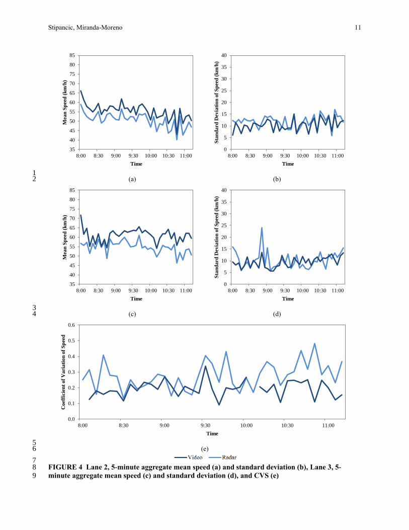
Temporal Speed Variation 11 The mean and standard deviation of speed was calculated for each 5-minute time interval and for every 12

lane across the entire collection period. The resultant plots for Lanes 2 and 3 are provided in Figure 4 as a 13

representative sample of the 5-lane arterial. Considering the mean speed, the overestimation bias of the 14

video-based sensor is apparent, with speeds that are consistently higher than those reported by the radar. 15

Regardless of this bias, the relative pattern of mean speeds collected by each detector is similar. This is an 16

important observation, as it is not necessarily high speeds, but high variation in speeds that make traffic 17

conditions unsafe. The standard deviation of speed, which is stable and consistent for both sensors, is 18

used to indicate the variation within the aggregation period itself. Despite the overestimation of speed 19

present in the video sensor, both devices show the same general trends in speed variation over time. 20

The CVS reported by both devices is plotted in Figure 4e. The peaks in the CVS plot indicate the 21

time periods in which collisions were most likely to occur. When considering only the mean and standard 22

deviation of speed, similarity between the detectors was observed. However, CVS was consistently higher 23

for the radar than for the video. As higher CVS is correlated with higher potential for collision, the radar 24

reports a lower level of safety compared to the video. The equation for CVS contains average speed in the 25

denominator. This means that, even with the same variation in speed, a higher average speed will result in 26

a lower CVS. The general overestimation of speed present in the video data will yield an underestimated 27

CVS compared to other sensors. In this case, the overestimation bias decreases the risk reported by the 28

device. The CVS results were compared using an analysis of variance (ANOVA). The ANOVA results 29

indicated that the CVS values for radar were statistically different than the video at 95% confidence (f = 30

25.6, p = 0.00). This confirms that CVS will exhibit significant differences when calculated using data 31

from different devices. 32

0

20

40

60

80

100

120

1 2 3 4 5 6 7 8 9 10

Cu

mu

lati

ve F

req

uen

cy

TTC (seconds)

Stipancic, Miranda-Moreno 11

1 (a) (b) 2

3 (c) (d) 4

5 (e) 6

7 FIGURE 4 Lane 2, 5-minute aggregate mean speed (a) and standard deviation (b), Lane 3, 5-8

minute aggregate mean speed (c) and standard deviation (d), and CVS (e) 9

35

40

45

50

55

60

65

70

75

80

85

8:00 8:30 9:00 9:30 10:00 10:30 11:00

Mea

n S

peed

(k

m/h

)

Time

0

5

10

15

20

25

30

35

40

8:00 8:30 9:00 9:30 10:00 10:30 11:00

Sta

nd

ard

Devia

tio

n o

f S

peed

(k

m/h

)

Time

35

40

45

50

55

60

65

70

75

80

85

8:00 8:30 9:00 9:30 10:00 10:30 11:00

Mea

n S

peed

(k

m/h

)

Time

0

5

10

15

20

25

30

35

40

8:00 8:30 9:00 9:30 10:00 10:30 11:00

Sta

nd

ard

Devia

tio

n o

f S

peed

(k

m/h

)

Time

0.0

0.1

0.2

0.3

0.4

0.5

0.6

8:00 8:30 9:00 9:30 10:00 10:30 11:00

Co

eff

icie

nt

of

Va

ria

tio

n o

f S

peed

Time

Stipancic, Miranda-Moreno 12

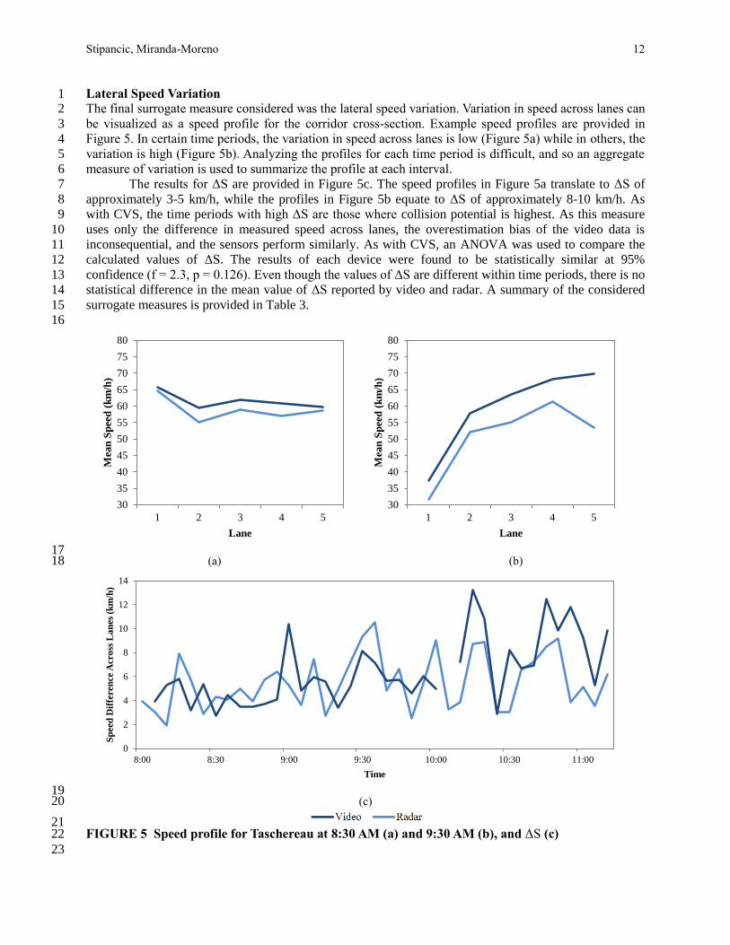
Lateral Speed Variation 1 The final surrogate measure considered was the lateral speed variation. Variation in speed across lanes can 2

be visualized as a speed profile for the corridor cross-section. Example speed profiles are provided in 3

Figure 5. In certain time periods, the variation in speed across lanes is low (Figure 5a) while in others, the 4

variation is high (Figure 5b). Analyzing the profiles for each time period is difficult, and so an aggregate 5

measure of variation is used to summarize the profile at each interval. 6

The results for ΔS are provided in Figure 5c. The speed profiles in Figure 5a translate to ΔS of 7

approximately 3-5 km/h, while the profiles in Figure 5b equate to ΔS of approximately 8-10 km/h. As 8

with CVS, the time periods with high ΔS are those where collision potential is highest. As this measure 9

uses only the difference in measured speed across lanes, the overestimation bias of the video data is 10

inconsequential, and the sensors perform similarly. As with CVS, an ANOVA was used to compare the 11

calculated values of ΔS. The results of each device were found to be statistically similar at 95% 12

confidence (f = 2.3, p = 0.126). Even though the values of ΔS are different within time periods, there is no 13

statistical difference in the mean value of ΔS reported by video and radar. A summary of the considered 14

surrogate measures is provided in Table 3. 15

16

17 (a) (b) 18

19 (c) 20

21 FIGURE 5 Speed profile for Taschereau at 8:30 AM (a) and 9:30 AM (b), and ΔS (c) 22

23

30

35

40

45

50

55

60

65

70

75

80

1 2 3 4 5

Mea

n S

pee

d (

km

/h)

Lane

30

35

40

45

50

55

60

65

70

75

80

1 2 3 4 5

Mea

n S

pee

d (

km

/h)

Lane

0

2

4

6

8

10

12

14

8:00 8:30 9:00 9:30 10:00 10:30 11:00

Sp

eed

Dif

feren

ce

Acro

ss L

an

es

(km

/h)

Time

Stipancic, Miranda-Moreno 13

TABLE 3 Summary of Surrogate Safety Measures Reported by Three Sensors 1

2

Device

Video Radar Magnetometer

TTC

# >3 seconds 30 10 9

# >5 Seconds 51 23 16

CVS

% Highest 19% 81% -

Highest Value 0.34 0.48 -

ΔS

% Highest 57% 43% -

Highest Value 13.21 10.49 -

note: bolded values indicate the highest reported level of risk for a surrogate measure 3

4

CONCLUSIONS 5 This paper endeavoured to evaluate three mobile traffic sensors in reporting traffic parameter safety 6

surrogates. For rear-end TTC, the video-based sensor found relatively more conflicts at TTC less than 3 7

and 5 seconds. The increased number of conflicts equates to a greater estimated risk compared to the 8

other sensors. The radar and magnetometer performed more similarly, with nearly equal number of 9

conflicts for TTC less than 3 seconds, though the radar reported more conflicts for TTC less than 5 10

seconds. Although video may slightly overestimate the number of conflicts, it is more likely that the other 11

sensors underestimate conflicts due to omitted speed measurements. Therefore, calculating TTC with data 12

from radar or magnetometer devices should account for the possible underestimation. 13

For temporal speed variation, consideration of only mean and standard deviation of speed 14

revealed approximately equivalent results from the radar and video sensors. However, when using CVS to 15

quantify speed variation, the variation indicated by the radar was consistently higher than for the video. 16

As CVS contains average speed in the denominator of the formulation, the overestimation of video-based 17

speeds reduced the reported CVS, resulting in lower reported risk when compared to the radar. The radar 18

reported the highest CVS in 81% of the time periods, and also reported the highest CVS overall. An 19

ANOVA analysis confirmed that differences in the results for both sensors were statistically significant. 20

While both TTC and CVS are indicators of the potential for rear end collisions, the results from the two 21

are contradictory. Under a TTC analysis, the video sensor will report the highest risk for rear end 22

collisions, while under a CVS analysis the radar will report the highest risk. As general overestimation 23

bias is a known issue with video-extracted speed data, CVS should not be calculated based on video data, 24

unless the bias can be removed, as suggested by Anderson-Trocme, Stipancic, and Miranda-Moreno (8). 25

Removing the overestimation bias would help to ensure the accuracy of all surrogates considered herein. 26

In general, if video data is used, care should be taken to select surrogates independent of mean speed. As a 27

general bias does not appear in the radar or magnetometer, the examined surrogates are appropriate for 28

use with these devices. 29

Utilizing the average difference in speed across lanes to quantify lateral speed variation is 30

independent of mean speed, the overestimation bias of the video is inconsequential, and the results from 31

both detectors are similar as expected. The measure is intuitive, as nearly flat speed profiles equate to low 32

ΔS values, while more varied profiles yield high ΔS values. Though the video reported the highest ΔS in 33

57% of the time periods and had the highest ΔS overall, an ANOVA analysis demonstrated no statistical 34

difference in the results of both detectors. 35

Stipancic, Miranda-Moreno 14

With these results considered, accurately quantifying safety requires selecting both an appropriate 1

surrogate measure, and selecting an appropriate device to collect the surrogate data. An ideal method 2

should consider multiple surrogate measures to improve the redundancy of the surrogate analysis. 3

Additionally, practitioners should use devices that are well understood, and that have been implemented 4

successfully in the past. Surrogate data collected over multiple sites should use the same sensor across all 5

sites, or better yet, use a combination of sensors to account for any biases that may be present in the 6

devices themselves. Future work should most importantly investigate more opportunities for 7

incorporating microscopic vehicle data into surrogate safety analysis, and should incorporate ground truth 8

sampling where possible to validate the sensor results. 9

10

ACKNOWLEDMENT 11 Funding for this project was provided in part by the Natural Science and Engineering Research Council. 12

Stipancic, Miranda-Moreno 15

REFERENCES 1

1. Lu, M. Modelling the effects of road traffic safety measures. Accident Analysis and Prevention, no.

38, 2007, pp. 507-517.

2. Bahler, S. J., J. M. Kranig, and E. D. Minge. Field Test of Nonintrusive Traffic Detection

Technologies. Transportation Research Record: Journal of the Transportation Research Board, no.

1643, 1998, pp. 161-170.

3. Abdel-Aty, M., and A. Pande. Identifying crash propensity using specific traffic speed conditions.

Journal of Safety Research, no. 36, 2005, pp. 97-108.

4. Lee, C., B. Hellinga, and K. Ozbay. Quantifying effects of ramp metering on freeway safety. Accident

Anaysis and Prevention, no. 38, 2006, pp. 279-288.

5. Tarko, A., G. Davis, N. Saunier, T. Sayed, and S. Washington. Surrogate Measures of Safety.

Transportation Research Board, 2009.

6. Gettman, D., and L. Head. Surrogate Safety Measures from Traffic Simulation Models.

Transportation Research Record: Journal of the Transportation Research Board, no. 1840, 2003, pp.

104-115.

7. Saunier, N., and T. Sayed. Automated Analysis of Road Safety. Transportation Research Record:

Journal of the Transportation Research Board, no. 2019, 2007, pp. 57-64.

8. Anderson-Trocme, P., J. Stipancic, and L. Miranda-Moreno. Performance Evaluation and Error

Segregation of Video-Collected Traffic Speed Data. in Transportation Association Annual

Conference Proceedings, Montreal, 2014.

9. Yan, X., M. Abdel-Aty, E. Radwan, X. Wang, and P. Chilakapati. Validating a driving simuator using

surrogate safety measures. Accident Analysis and Prevention, no. 40, 2008, pp. 274-288.

10. Oh, C., J.-s. Oh, and S. G. Ritchie. Real-time estimation of Freeway Accident Likelihood. in

Transportation Research Board Annual Meeting, Washington, D.C., 2001.

11. U.S. Department of Transportation Federal Highway Administration. Field Test of Monitoring of

Urban Vehicle Operations Using Non-Intrusive Technologies. 1997.

12. Lee, C., F. Saccomanno, and B. Hellinga. Analysis of Crash Precursors on Instrumented Freeways.

Transportation Research Record: Journal of the Transportation Research Board, no. 1784, 2002, pp.

1-8.

13. Golob, T. F., W. W. Recker, and V. M. Alvarez. Freeway safety as a function of traffic flow. Accident

Analysis and Prevention, no. 36, 2004, pp. 933-946.

14. Davis, G. A. Is the claim that 'variance kills' an ecological fallacy? Accident Analysis and Prevention,

no. 34, 2002, pp. 343-346.

15. Skszek, S. L. "State-of-the-Art" Report on Non-Traditional Traffic Counting Methods. Arizona

Department of Transportation, Pheonix, AZ, 2011.

16. Stipancic, J., S. Burns, and L. Miranda-Moreno. A testing protocol and performance evaluation of

mobile traffic data collection technologies in an urban context. in Canadian Society of Civil

Engingeers Annual Conference Proceedings, Halifax, 2013.

17. van der Horst, A.R. A., M. de Goede, S. de Hair-Buijssen, and R. Methorst. Traffic conflicts on

bicycle paths: A systematic observation ofbehaviour from video. Accident Analysis and Prevention,

no. 62, 2014, pp. 358-368.

18. Laureshyn, A., and H. Ardo. Automated video analysis as a tool for analysing road user behaviour. in

Proceedings of ITS World Congress, London, 2006.

3