1

Traffic Network Control from Temporal LogicSpecifications

Samuel Coogan, Ebru Aydin Gol, Murat Arcak, and Calin Belta

Abstract—We propose a framework for generating a signalcontrol policy for a traffic network of signalized intersections toaccomplish control objectives expressible using linear temporallogic. By applying techniques from model checking and formalmethods, we obtain a correct-by-construction controller thatis guaranteed to satisfy complex specifications. To apply thesetools, we identify and exploit structural properties particularto traffic networks that allow for efficient computation of afinite state abstraction. In particular, traffic networks exhibita componentwise monotonicity property which allows reach setcomputations that scale linearly with the dimension of thecontinuous state space.

I. INTRODUCTION

State-of-the-art approaches to coordinated control of sig-nalized intersections often focus on limited objectives such asmaximizing throughput [1] or maintaining stability of networkqueues [2], [3]; see [4] for a review of the literature. However,traffic networks are a natural domain for a much richer classof control objectives that are expressible using linear temporallogic (LTL) [5], [6]. LTL formulae allow control objectivessuch as “actuate traffic flows such that throughput is alwaysgreater than C1” where C1 is a threshold throughput, or suchthat “traffic link queues are always less than C2” where C2

is a threshold queue length. LTL formulae also allow morecomplex objectives such as “infinitely often, the queue lengthon road ` should reach 0,” “anytime link ` becomes congested,it eventually becomes uncongested,” or any combination ofthese conditions. As these examples suggest, many objectivesthat are difficult or impossible to address using standardcontrol theoretic techniques are easily expressed in LTL.

In this paper, we propose a technique for synthesizing asignal control policy for a traffic network such that the networksatisfies a given control objective expressed using LTL. Thesynthesized policy is a finite-memory, state feedback controllerthat is provably correct, that is, guaranteed to result in a closedloop system that satisfies the control objective.

Recent approaches to control synthesis from LTL specifica-tions such as [7]–[21] allow automatic development of correct-by-construction control laws; however, despite these promisingdevelopments, scalability concerns prevent direct applicationof existing results to large traffic networks.

This research was supported in part by the NSF under grants CNS-1446145 and CNS-1446151. Samuel Coogan and Murat Arcak are with theDepartment of Electrical Engineering and Computer Sciences, University ofCalifornia, Berkeley, {scoogan,arcak}@eecs.berkeley.edu. EbruAydin Gol is formerly with the Division of Systems Engineering, BostonUniversity, ebruaydin@gmail.com. Calin Belta is with the Departmentof Mechanical Engineering, Boston University, cbelta@bu.edu

To overcome these scalability limitations, we identify andexploit componentwise monotonicity [22] properties inherentin flow networks such as traffic networks. These properties al-low efficient computation of bounds on the one-step reachableset from a rectangular box of initial conditions, which in turnallows efficient computation of a finite state abstraction of thedynamics, thereby mitigating a crucial bottleneck in the controlsynthesis process. A related approach to abstractions of mono-tone systems is suggested in [23], however the componentwisemonotonicity properties exploited in this work are much moregeneral and encompass monotone systems as a special case.The present paper builds on our preliminary work in [24] bydefining componentwise monotonicity and identifying it as theenabling property for efficient abstraction.

This paper is organized as follows: Section II gives nec-essary preliminaries. Section III presents the model for sig-nalized networks, and Section IV establishes the problemformulation. Section V identifies componentwise monotonicityproperties of the traffic networks, and Section VI presentsscalable algorithms that rely on these properties to constructa finite state representation of the traffic network. Section VIIdescribes the controller synthesis approach, and discusses thecomputation requirements of our method. We present a casestudy in Section VIII and conclude our work in Section IX.

II. PRELIMINARIES

The set I ⊆ Rn is a box if it is the cartesian product ofintervals, or equivalently, I is a box if there exists x, y ∈ Rnsuch that I =

∏ni=1{z ∈ R | xi ≺1

i z ≺2i yi} where ≺1

i

,≺2i∈ {<,≤} and xi, yi denote the ith coordinate of x and y,

respectively. Defining ≺1, {≺1i }ni=1 and ≺2, {≺2

i }ni=1, wemay write I = {z ∈ Rn | x ≺1 z ≺2 y}. The vector x is thelower corner of I, and likewise y is the upper corner.

When applied to vectors, <, ≤, >, and ≥ are interpretedelementwise. The notation 0 denotes the all-zeros vector wherethe dimension is clear from context. We denote closure of a setY by cl(Y ). Given an index set L and a set of values x` ∈ Rfor ` ∈ L, {x`}`∈L denotes the collection of x`, ` ∈ L, butwe also interpret x = {x`}`∈L as an element of R|L|.

A transition system is a tuple T = (Q,S,→) where Q isa finite set of states, S is a finite set of actions, and →⊂Q×S×Q is a transition relation. We write q s→ q′ instead of(q, s, q′) ∈→. Note that all transition systems in this paper arefinite [6]. The evolution of a transition system is described by→. That is, a transition system is initialized in some state q0 ∈Q, and, given an action s ∈ S, the next state of the transitionsystem is chosen nondeterministically from {q′ | q s→ q′}.

2

1 ` 1032 76

54 98

Fig. 1. A typical traffic network with 11 links and 7 signalized intersections.In the figure, Ldown

` = {`, 7, 8, 10}, Lup` = {1, 2, 5}, and Ladj

` = {3, 4}. Ateach time step, a signal actuates a subset of upstream links.

III. SIGNALIZED NETWORK TRAFFIC MODEL

A signalized traffic network consists of a set L of links anda set V of signalized intersections. For ` ∈ L, let η(`) ∈ Vdenote the downstream intersection of link ` and let τ(`) ∈V ∪∅ denote the upstream intersection of link `. A link ` withτ(`) = ∅ serves as an entry-point into the network, and weassume η(`) 6= τ(`) for all ` ∈ L (i.e., no self-loops). Linkk 6= ` is upstream of link ` if η(k) = τ(`), downstream of link` if τ(k) = η(`), and adjacent to link ` if τ(k) = τ(`). Roadsexiting the traffic network are not modeled explicitly. For eachv ∈ V , define Lin

v = {` | η(`) = v}, Loutv = {` | τ(`) = v}

and for each ` ∈ L, define

Lup` = {k ∈ L | η(k) = τ(`)} (1)

Ldown` = {k ∈ L | τ(k) = η(`)} ∪ {`} (2)

Ladj` = {k ∈ L | τ(k) = τ(`)}\{`} (3)

so that Ldown` includes link ` and the links downstream of link

`, and Lup` and Ladj

` are the links upstream and adjacent to`, respectively, see Fig. 1. We have Ldown

` ∩ Ladj` = ∅ and

Lup` ∩L

adj` = ∅, but note that it is possible for Ldown

` ∩Lup` 6= ∅,

in particular, if there is a cycle of length two in the network.Let Lloc

` = Ldown` ∪ Lup

` ∪ Ladj` be links “local” to link `.

Each link ` ∈ L possesses a queue x`[t] ∈ [0, xcap` ]

representing the number of vehicles on link ` at time stept ∈ N , {0, 1, 2, . . .} where xcap

` is the capacity of link `. Weallow x` to be a continuous quantity, thus adopting a fluid-likemodel of traffic flow evolving in slotted time as in [1]–[3].

Movement of vehicles among link queues is governedby mass-conservation laws and the state of the signalizedintersections. A link is said to be actuated if outgoing flowfrom link ` is allowed as determined by the state of the trafficsignal at intersection η(`). At each intersection v,

Sv ⊆ 2Linv (4)

denotes the set of available signal phases, that is, each sv ∈ Sv ,sv ⊆ Lin

v denotes a set of incoming links at intersection v thatmay be actuated simultaneously. We define

S = {∪v∈Vsv | sv ∈ Sv ∀v ∈ V} ⊆ 2L (5)

so that each s ∈ S, s ⊆ L denotes a set of links in the networkthat may be actuated simultaneously. We identify s ∈ S withits constituent phases so that s = {sv}v∈V , and we interpretS as the set of allowed inputs to the traffic network.

When a link is actuated, a maximum of c` vehicles areallowed to flow from link ` to links Lout

η(`) per time step where

c` is the known saturation flow for link `, [4]. The turn ratioβ`k denotes the fraction of vehicles exiting link ` that arerouted to link k, [2]. Then β`k 6= 0 only if η(`) = τ(k), and∑

k∈Loutη(`)

β`k ≤ 1. (6)

Strict inequality in (6) implies that a fraction of vehicles onlink ` are routed off the network via unmodeled roads that exitthe network. Traffic flow can occur only if there is availablecapacity downstream. To this end, the supply ratio αsv`k denotesthe fraction of link k’s capacity available to link ` during phasesv ∈ Sτ(k). That is, link ` may only send αsv`k(xcap

k − xk[t])vehicles to link k in time period t under input sv . As the supplyis only divided among actuated incoming links, it follows thatfor each k ∈ L∑

`∈sv

αsv`k = 1 ∀sv ∈ Sτ(k), sv 6= ∅. (7)

Constant turn and supply ratios are a common modelingassumption justified by empirical observations; see [25] forfurther discussion.

We are now in a position to define the dynamics of the linkqueues. As we will see subsequently, the flow of vehicles outof link ` is only a function of the state of links in Ldown

` , andthe update of link `’s state is only a function of links in Lloc

` .Let x[t] = {x`[t]}`∈L, xdown

` [t] = {xk[t]}k∈Ldown`

, andxloc` [t] = {xk[t]}k∈Lloc

`. The outflow of link ` ∈ L is as follows:

f out` (xdown

` , sη(`)) =min

{x`[t], c`,min k s.t.

β`k 6=0

{αsη(`)`k

β`k(xcapk − xk[t])

}}if ` ∈ sη(`)

0 else.

(8)

The interpretation of (8) is that the flow of vehicles exitinga link ` when actuated is the minimum of the link’s queuelength, its saturation flow, and the downstream supply of ca-pacity, weighted appropriately by turn and supply ratios. Thismodeling approach is based on the cell transmission modelof traffic flow [26] which restricts flow if there is inadequatecapacity downstream. A consequence of (8) is that inadequatecapacity on one downstream link at an intersection causescongestion that blocks incoming flow to other downstreamlinks. This phenomenon, sometimes called the first-in-first-out property, has been widely studied in the transportationliterature and occurs even in multilane settings [27]1. Thenumber of vehicles in each link’s queue then evolves accordingto the mass conservation equation

x`[t+ 1] =F`(xloc` [t], sloc

` [t], d`[t]) (9)

,min{xcap` , x`[t]− f out

` (xdown` [t], sη(`))

+∑j∈Lup

`

βj`foutj (xdown

j [t], sη(j)) + d`[t]}

(10)

1Even if a turn pocket exists at an intersection, it is often too short to fullymitigate this blocking property. Nonetheless, if the road geometry is suchthat a sufficient number of dedicated lanes exist for a turning movement,these lanes may be modeled with a separate link.

3

where d`[t] is the number of vehicles that exogenously entersthe queue on link ` in time step t, d = {d`[t]}`∈L, and sloc

` ={sη(`), sτ(`)} if τ(`) 6= ∅, sloc

` = {sη(`)} otherwise; that is,sloc` is the state of the signals that are “local” to link `. The

minimization in (10) is only needed in case the exogenousinput d`[t] would cause the state of link ` to exceed xcap

` andensures that the network dynamics maps

X =∏`∈L

[0, xcap` ] (11)

to itself. We interpet this as refusal of vehicles attempting toexogenously enter the network when the link is full. Notein particular that the supply/demand formulation preventsupstream inflow from exceeding supply and thus for links withno exogenous input, xcap

` is never the unique minimizer in (10).

Remark 1. An alternative to the above approach is to define anauxiliary sink state Out in the transition systems T defined inSection VI which captures any trajectories that exit the domainX . The temporal logic specification can then incorporate therequirement that the system never enters this Out state.

Assumption 1. We assume there exists D ⊂ RL such that

d[t] ∈ D ∀t (12)

and D satisfies D ⊂ ∪nDi=1Di where each Di is given by

Di = {d | di ≤ d ≤ di} (13)

for some di = {di`}`∈L, di

= {di`}`∈L.

In other words, we assume the disturbance is containedwithin a union of boxes given by (13). This assumption is notparticularly restrictive, as any compact subset of RL can beapproximated with boxes to arbitrary precision [28], howeverthe number of boxes nD affects the computation time asdetailed in Section VII-B.

We let F (x, s,d) = {F`(xloc` , s

loc` , d`)}`∈L : X ×S ×D →

X so that

x[t+ 1] = F (x[t], s[t],d[t]). (14)

The set of states of system (14) that are reachable from aset Y ⊂ X under the control signal s ∈ S in one timestep isdenoted by the Post operator and given by

Post(Y, s) = {x′ = F (x, s,d) | x ∈ Y,d ∈ D}. (15)

We call Post(Y, s) the one step reachable set from Y unders. The main features of the queue-based modeling approachproposed above such as finite saturation rates, finite queuecapacity, a set of available signaling phases, and fixed turn ra-tios are standard in many modeling and simulation approachessuch as [2], [3], see also [4], [29] and references therein fordiscussions of queue-based modeling of traffic networks.

IV. PROBLEM FORMULATION AND APPROACH

We now define and motivate the need for control objectivesexpressible in LTL for traffic networks, and we outline acontrol synthesis approach which relies on a finite staterepresentation of the traffic dynamics to meet these objectives.

LTL formulae are generated inductively using the Booleanoperators ∨ (disjunction), ∧ (conjunction), ¬ (negation), andthe temporal operators # (next) and U (until). From these, weobtain a suite of derived logical and temporal operators suchas→ (implication), � (always), ♦ (eventually), �♦ (infinitelyoften), finite deadlines with repeated #, and many others, see[5], [6].

Formally, such formulae are expressed over a set of atomicpropositions, which we restrict to be indicator expressionsover subsets of X or predicates over the signaling state. Forexample, the atomic proposition x` ≤ 10 is true for all x ∈ Xthat satisfies the condition x` ≤ 10 (which constitutes a boxsubset of X ), and the atomic proposition ` ∈ s is true for allsignals that actuate link `. We will see in Section V and SectionVI that restricting to atomic propositions corresponding to boxsubsets of X offers significant computational advantages.

Semantically, LTL formulae are interpreted over a trajectoryx[t] and the corresponding input sequence s[t] for t = 0, 1, . . ..For example, the state/input sequence (x[t], s[t]) satisfies theLTL formula ϕ = �(x` ≤ 10) ∧ �♦(` ∈ s) if and only ifx`[t] ≤ 10 for all t and ` ∈ s[t] infinitely often (i.e., forinfinitely many t). Thus a trajectory satisfies a LTL formulaif and only if the formula holds for the corresponding traceof atomic propositions that are valid at each time step. Aformal definition of the semantics of LTL over traces is readilyavailable in the literature, e.g., [5], [6], and is a naturalinterpretation of the above Boolean and temporal operators.For example, a trace satisfies ♦ϕ if and only if there exists asuffix of the trace satisfying ϕ.

Examples of LTL formulae representing desired controlobjectives relevant to traffic networks include those from theIntroduction, as well as:• ϕ1 = ♦�(x` ≤ C) for some C

“Eventually, link ` will have less than C vehicles and thiswill remain true for all time”

• ϕ2 = �♦(` ∈ s)“Infinitely often, link ` is actuated”

• ϕ3 = �((` ∈ sv1)→#(k ∈ sv2))“Whenever signal v1 actuates link `, signal v2 must actuatelink k in the next time step”

• ϕ4 = �(x` ≥ C1→ ♦(x` ≤ C2))“Whenever the number of vehicles on link ` exceeds C1, itis eventually the case that the number of vehicles on link `decreases below C2.”

The main problem considered in this paper is as follows:

Control Synthesis Problem. Given a traffic network and anLTL formula ϕ over a set of atomic propositions as describedabove, find a control strategy that, at each time step, chooses asignaling input such that all trajectories of the traffic networksatisfy ϕ from any initial condition.

To solve the control synthesis problem, we propose com-puting a finite state abstraction that simulates (in a mannerto be formalized below) the traffic network dynamics. As wediscuss in Section VII-A, the result is a full-state feedbackcontroller which requires finite memory. We rely on dynamicalproperties of the traffic network to compute the abstraction,and then apply tools from automata theory and formal methods

4

to synthesize a finite-memory, state feedback control strategysolving the control synthesis problem.

V. COMPONENTWISE MONOTONICITY OF TRAFFICNETWORKS

To generate control strategies for the traffic network thatguarantee satisfaction of a LTL formula, we first construct afinite state representation, or abstraction, of the model definedin Section III. We now define a componentwise monotonicityproperty that simplifies this task and next show that the modelin Section III possesses this property.

Definition 1. Consider the dynamical system

z[t+ 1] = f(z[t], w[t]) (16)

for z ∈ Z ⊆ Rn, w ∈ W ⊆ Rm with f : Z×W → Z contin-uous. System (16) is componentwise monotone if there existsa signature matrix ∆ = [δij ]

ni,j=1 with each δij ∈ {−1, 1}

such that for all i,

δijξj ≤ δijξj and wj ≤ wj ∀j ∈ L (17)

implies f(ξ, w) ≤ f(ξ, w)) (18)

for any ξ, ξ ∈ Z , w,w ∈ W . That is, (16) is componentwisemonotone if fi is monotonic in each z variable and monoton-ically increasing in each w variable.

A definition similar to Definition 1 appears in [22], but omitsdependence on a disturbance input.

We now give a characterization of componentwise mono-tone systems which stipulates that ∂f/∂z be sign-stable, thatis, the sign structure of the Jacobian does not change as z, wrange over their domain.

Lemma 1. Consider dynamical system (16) and further sup-pose that f(z, w) =

[f1(z, w) . . . fn(z, w)

]Tis Lipschitz

continuous so that partial derivatives exist almost everywhere.If for all i ∈ {1, . . . , n}:

∀j ∈ {1, . . . , n} ∃δij ∈ {−1, 1} : δij∂fi∂zj

(z, w) ≥ 0 a.e. (19)

and ∀j ∈ {1, . . . ,m} :∂fi∂wj

(z, w) ≥ 0 a.e. (20)

where a.e.(almost everywhere) implies the condition must holdwherever the derivative exists, then (16) is componentwisemonotone.

Proof. Let [δij ]ni,j=1 be as in the hypothesis of the Lemma.

By the Fundamental Theorem of Calculus, for all w and foralmost all2 ξ, ξ satisfying δijξj ≤ δijξj for all j,

fi(ξ, w)− fi(ξ, w) = (21)(∫ 1

0

∑nj=1

∂fi∂ξj

(ξ + r(ξ − ξ), w)(ξj − ξj)dr)≥ 0 (22)

where nonnegativity follows because δij(ξj − ξj) ≥ 0,

δij∂fi/∂ξj ≥ 0, and δ2ij = 1 for all i, j. Similarly, for almost

2Eq. (21) requires existence of ∂g/∂z almost everywhere along the linesegment connecting z and z, which holds for almost all z for fixed z [30,Ch. 2]. Similarly, fi(ξ, w)− fi(ξ, w) holds for almost all w for fixed w.

all w ≥ w, fi(ξ, w) − fi(ξ, w) ≥ 0. It follows by continuityof fi that fi(ξ, w) − fi(ξ, w) ≥ 0 for all ξ, ξ that satisfyδijξj ≤ δijξj and all w ≤ w, for all i, completing theproof.

The critical feature of componentwise monotone systemswe wish to exploit is that over approximating the one-stepreachable set from a box of initial conditions is computation-ally efficient. In particular, the reach set is contained withina box defined by the value of fi at two particular points foreach i, regardless of the dimension of the spaces Z and W:

Lemma 2. Let (16) be componentwise monotone with signa-ture matrix ∆ = [δij ]

ni,j=1 and assume Z is a closed box.

Given z, z ∈ Z and w,w ∈ W with z ≤ z and w ≤ w. Letξi ∈ Z and ξ

i ∈ Z be defined elementwise as follows for eachi:

ξij

=

{zj if δij = 1

zj if δij = −1, ξ

i

j=

{zj if δij = 1

zj if δij = −1.(23)

Then

fi(ξi, w) ≤ fi(z, w) ≤ fi(ξ

i, w) ∀i (24)

for all z, w such that z ≤ z ≤ z and w ≤ w ≤ w.

Proof. Observe that δijξij ≤ δijzj for all i, j for all z ≤ z ≤ z,

and symmetrically, δijzj ≤ δijξi

j for all i, j for all z ≤ z ≤ z.The Lemma then follows immediately from Definition 1.

This remarkable feature of componentwise monotone sys-tems is analogous to well-known results for monotone systems[31]–[33], but componentwise monotonicity allows consider-ation of a much broader class of systems, including trafficnetworks, which are generally not monotone.Remark 2. Observe that the lower and upper bounds in (24)are achieved for appropriate choice of z and w, thus theapproximation of the one-step reachable set is tight.

To prove that the traffic network dynamics developed inSection III are componentwise monotone, we first require atechnical assumption:

Assumption 2. For all ` ∈ L,

c` ≤ xcap` −

βk`αk`

ck ∀k ∈ Lup` . (25)

Assumption 2 is a sufficient condition for ensuring that ifa link has inadequate capacity and blocks upstream flow, thenthis link’s queue will not empty in one time step. This effec-tively is an assumption that the time step is sufficiently smallto appropriately capture the queuing phenomenon. Specifically,the saturation flow rate c` of link ` is in units of vehicles pertime step and, thus, is implicitly a function of the chosen timestep. Physically, c` is required to decrease with decreased timestep and thus Assumption 2 is satisfied when a sufficientlysmall time step is used for the model.

Theorem 1. The traffic network model is componentwisemonotone for any signaling input s ∈ S. In particular, F`is increasing in xk for k downstream or upstream of link ` orequal to `, and decreasing in xk for k adjacent to link `.

5

Proof. For fixed s ∈ S, we show that F (x, s,d) satisfiesconditions (19) and (20) of Lemma 1 with x,d replacingz, w. Observe that F is continuous and piecewise differentiableby (8)–(10) and (14), thus it is Lipschitz continuous [34].The minimum function in (8) implies that F is differentiablealmost everywhere. We first have ∂F`

∂d`∈ {0, 1} a.e. by (10),

satisfying (20). Now consider ∂F`/∂xk. For (20), we considerfour exhaustive cases:• Case 1, k ∈ (Ldown

` ∪ Lup` )\{`}. From (8)–(10), link k may

block the outflow of link ` when k ∈ Ldown` , or link k may

contribute to the inflow to link ` if k ∈ Lup` , thus we have

∂F`∂xk

∈ {0,−∂fout`

∂xk, βk`

∂f outk

∂xk,−∂f

out`

∂xk+ βk`

∂f outk

∂xk} a.e. where

the fourth possibility occurs only if k ∈ Ldown` ∩ Lup

` . But∂f out`

∂xk∈ {0,−αsη(`)`k /β`k} a.e. and ∂f out

k

∂xk∈ {0, 1} a.e., thus

∂F`∂xk≥ 0 a.e., satisfying (19).

• Case 2, k = `. We have ∂f out`

∂x`∈ {0, 1} a.e. and, for j ∈ Lup

` ,∂f outj

∂x`∈ {0, αsη(j)j` /βj`} a.e., however, Assumption 2 ensures

that, a.e., either ∂f out`

∂x`= 0 or ∂f in

`

∂x`= 0, i.e.,

∂f outj

∂x`= 0 for all

j ∈ Lup` . Thus ∂F`

∂x`∈ {0, 1, 1 +

∑j∈Lup

`βj`

∂f outj

∂x`} a.e. But∑

j∈Lup`βj`

∂f outj

∂x`≥ −

∑j∈Lup

`αsη(j)j` = −1 by (7) (recall

that η(j) = τ(`) for all j ∈ Lup` ), that is, ∂f in

` /∂x` ≥ −1,thus ∂F`

∂x`≥ 0 a.e., satisfying (19).

• Case 3, k ∈ Ladj` . In this case, inadequate capacity of link

k may block flow to link `, as discussed above. We have∂F`∂xk

=∑j∈Lup

`βj`

∂f outj

∂xk. Since

∂f outj

∂xk∈ {0,−αsη(j)jk /βjk}

a.e., we have ∂F`∂xk≤ 0 a.e., satisfying (19).

• Case 4, k 6∈ Lloc` . Then ∂F`

∂xk= 0, trivially satisfying (19).

The following corollary implies that the one-step reachableset of the traffic dynamics from a (closed) box I for any givensignaling input s is over-approximated by the union of boxes,one box for each i = 1, . . . nD, where each of these boxesis efficiently computed by evaluating F` at two particularpoints for each ` ∈ L. The obtained over-approximation isdenoted with the Post operator. This critical result allowsefficient computation of a finite state representation of thetraffic dynamics, as detailed in Section VI.

Corollary 1. Consider the set I = {x | x ≤ x ≤ x}for x,x ∈ X , and for each ` ∈ L, define ξ`(x,x) =

{ξ`k(xk, xk)}k∈Lloc

`, ξ

`(x,x) = {ξ`k(xk, xk)}k∈Lloc

`where

ξ`k(xk, xk) =

{xk if k ∈ Ldown

` ∪ Lup`

xk if k ∈ Ladj`

(26)

ξ`

k(xk, xk) =

{xk if k ∈ Ldown

` ∪ Lup`

xk if k ∈ Ladj` .

(27)

Then for all s ∈ S, Post(I, s) ⊆ Post(I, s) where

Post(I, s) :=nD⋃i=1

{x′ | F`(ξ`, sloc` , d

i`) ≤ x′` ≤ F`(ξ

`, sloc` , d

i

`) ∀` ∈ L}.

(28)

q9 q10 q11 q12

q5 q6 q7 q8

q1 q2 q3 q4

xmax`

xmaxk

xmax`

xmaxk

q1

q4q5

q2 q3

q6

(a) (b)Fig. 2. Stylized depictions of two box partitions. (a) A gridded box partitionwith regularly sized intervals. (b) A nongridded box partition.

Proof. By substituting x,x for z, z and di`, di

` for w,w inLemma 2 and defining f(x,d) , F (x, s,d), we obtain {x′ =F (x, s,d) | x ∈ I,d ∈ Di} ⊆ {x′ | F`(ξ`, sloc

` , di`) ≤ x′` ≤

F`(ξ`, sloc` , d

i

`) ∀` ∈ L} for all i = 1, . . . , nD. The corollaryfollows from the trivial fact that Post(I, s) = ∪nDi=1{x′ =F (x, s,d) | x ∈ I, d ∈ Di}.

VI. FINITE STATE REPRESENTATION

To apply the powerful tools of LTL synthesis, we requirea finite state representation of the traffic network model. Ingeneral, obtaining finite state abstractions is a difficult problemand existing techniques do not scale well. In this section, weexploit the componentwise monotonicity properties developedabove and propose an efficient method for determining a finitestate representation of the traffic network dynamics.

A. Finite State Abstraction

Definition 2 (Box partition). For finite index set Q, the set{Iq}q∈Q is a box partition of X (or simply a box partition),if each Iq ⊆ X is a box, ∪q∈QIq = X , and Iq ∩ Iq′ = ∅ forall q, q′ ∈ Q. For q ∈ Q, let xq = {xq,`}`∈L, xq = {xq,`}`∈Ldenote the lower and upper corners, respectively, of Iq , thatis, Iq = {x | xq ≺1

q x ≺2q xq} where ≺1

q= {≺1q,`}`∈L,

≺2q= {≺2

q,`}`∈L, and ≺1q,`,≺2

q,`∈ {<,≤}.

For a box partition {Iq}q∈Q of X , let π : X → Q beuniquely defined by the condition x ∈ Iπ(x), that is, π(·) isthe natural projection from the domain X to the (index setof) boxes. A special case of a box partition of a rectangulardomain is the following:

Definition 3 (Gridded box partition). For X = {x ={x`}`∈L | x` ≤ x` ≤ x`}, a box partition {Iq}q∈Q of Xis a gridded box partition if for each ` ∈ L, there existsN` ∈ {1, 2, . . .} and a set of intervals {I`1, . . . , I`N`} such that∪N`i=1I

`i = [x`, x`] and for each q ∈ Q, there exists indices

q` ∈ {1, . . . , N`} such that Iq =∏`∈L I

`q`

. For gridded boxpartitions, we make the identification Q ∼=

∏`∈L{1, . . . , N`}

for all ` ∈ L.

When a box partition is not a gridded box partition, we sayit is nongridded. Fig. 2 shows two examples of box partitions,one of which is a gridded box partition. From a box partitionof the traffic network domain X , we obtain a finite staterepresentation, or abstraction, of the traffic network model asfollows. Each element of the box partition corresponds to asingle state in the resulting finite state transition system, and

6

to obtain a computationally tractable approach, we propose amethod for efficiently obtaining a finite state abstraction usingthe componentwise monotonicity properties developed above:

Definition 4 (CM-induced finite state abstraction). Givena box partition {Iq}q∈Q of X , the nondeterministic com-ponentwise monotonicity-induced (CM-induced) finite stateabstraction, or simply the finite state abstraction, of the trafficmodel is the transition system T = (Q,S,→) where Q isthe index set of the box partition, S is the available signalinginputs, and → is defined by:

(q, s, q′) ∈→ if and only if Iq′ ∩ Post(cl(Iq), s) 6= ∅.(29)

Remark 3. We must take the closure of Iq in (29) as the Post

operator and relevant properties (e.g., (28)) assume a closedbox. This allows efficient algorithms for constructing → via(29) as detailed below.

Note that the CM-induced finite state abstraction is nonde-terministic. Nondeterminism arises from the disturbance inputd and from the fact that a collection of continuous states isabstracted to one discrete state.

By the definition of the finite state abstraction above, for anytrajectory x[t], t ∈ N generated by the traffic model underinput sequence s[t], t ∈ N, there exists a unique sequenceq[t], t ∈ N with each q[t] ∈ Q such that x[t] ∈ Iq[t] and

q[t]s[t]→ q[t+ 1]. A transition system satisfying this property is

said to be a discrete abstraction of the dynamical system (14).A controller synthesized from the abstraction to satisfy anLTL formula as described in Section V can be applied to theoriginal traffic network with the same guarantees because theabstraction simulates the original traffic network [6]. However,abstractions generally result in unavoidable conservatism, thatis, nonexistence of an appropriate control strategy from theabstraction does not imply nonexistence of a control strategyfor the original traffic network.

The following corollary to Remark 2 implies that the finitestate abstraction suggested in Definition 4 does not introduceexcessive conservatism; specifically, Corollary 2 tells us thatif (q, s, q′) ∈→, then for each link `, it is possible for the stateof link ` to transition from a state in box Iq to a state in Iq′ .

Corollary 2. For the CM-induced finite state abstractiondefined above, (q, s, q′) ∈→ if and only if

∃d = {d`}`∈L ∈ D,∃x′ = {x′`}`∈L ∈ Iq′ such that (30)

∀` ∈ L,∃x ∈ cl(Iq) s.t. x′` = F`(xloc` [t], sloc[t], d`[t]).

(31)

Proof. (if). Suppose (30)–(31) holds for some q, q′ ∈ Qand s ∈ S , and let d ∈ D and x′ ∈ Iq′ be a particularsolution such that (31) holds for all `. We will show thatx′ ∈ Post(cl(Iq), s). Let i∗ be such that d ∈ Di∗ , and let ξ`,

ξ`

be as in Corollary 1. We must have

F`(ξ`, sloc

` , di∗

` ) ≤ x′` ≤ F`(ξ`, sloc` , d

i∗

` ) (32)

by Lemma 2 where we make the same substitutions as in theproof of Corollary 1 because (24) holds for x satisfying (31)

1: function ABSTRACTION(network model, D, {Iq}q∈Q)returns T

2: inputs: network model, a traffic network model withupdate functions {F`}`∈L with domain Xand signal input set S

3: D, the disturbance set D = ∪nDi=1Di4: {Iq}q∈Q, a box partition X5: →:= ∅6: for each s ∈ S do7: for each q ∈ Q do8: for i := 1 to nD do9: ξ` := as in (26)

10: ξ`

:= as in (27)11: y := F`(ξ

`, sloc` , d

i`)

12: y := F`(ξ`, sloc` , d

i

`)13: Q′ := SUCCESSORS(y,y, {Iq}q∈Q)14: →:=→ ∪(q × s×Q′)15: end for16: end for17: end for18: return T := (Q,S,→)19: end functionFig. 3. Algorithm for computing a finite state abstraction of the trafficdynamics. The algorithm requires function SUCCESSORS, which can beimplemented using different algorithms, depending on the structure of thebox partition.

for each ` ∈ L. By (28), it follows that x′ ∈ Post(cl(Iq), s),and thus (q, s, q′) ∈→.

(only if). Suppose (q, s, q′) ∈→, it follows that Iq′ ∩Post(cl(Iq), s) 6= ∅, let x′ ∈ Iq′ ∩ Post(cl(Iq), s) andlet i∗ ∈ {1, . . . , nD} be such that F`(ξ`, sloc

` , di∗

` ) ≤ x′` ≤F`(ξ

`, sloc` , d

i∗

` ) for all ` ∈ L. Remark 2 implies that foreach `, there exists x ∈ cl(Iq) and d†` ∈ [di

∗

` , di∗

` ] such thatx′` = F`(x

loc` , s

loc` , d

†`). Indeed, suppose not, then

x` , supx∈cl(Iq),d`∈[di

∗` ,d

i∗` ]

F`(xloc` , s

loc` , d`) < x′`, or (33)

x˜` , inf

x∈cl(Iq),d`∈[di∗` ,d

i∗` ]

F`(xloc` , s

loc` , d`) > x′`. (34)

If (33) holds, then F`(x, s,d) ≤ x` < x′` ≤ F`(ξ`, sloc` , d

i∗

` )

for all xq ≤ x ≤ xq and all di∗≤ d ≤ di

∗

, which impliesthe upper bound in (24) is not achieved, contradicting the firststatement of Remark 2. A symmetric argument shows that if(34) holds, then Remark 2 is again contradicted. Defining d ={d†`}`∈L for the particular collection {d†`}`∈L above impliesthat (30)–(31) holds, completing the proof.

We remark that, in (31), the same choice of x ∈ cl(Iq) willgenerally not work for all ` ∈ L due to the over-approximationof the reachable set; see [24] for further discussion.

B. Constructing The Transition System TWe begin with the primary algorithm for calculating T

shown in Fig. 3, which relies on Corollary 1 to computePost and to construct the finite state abstraction as defined

7

in Definition 4. This algorithm requires a function calledSUCCESSORS that takes the lower and upper corners of abox Y as input, as well as a box partition of X , and returnsthe indices of the box partitions which intersects Y . We firstpresent a generic algorithm for SUCCESSORS applicable toany box partition. To this end, consider the nonempty boxIq = {x | x ≺1

q x ≺2q x} and let Y , {x | y ≤ x ≤ y}.

It is straightforward to show that Iq ∩ Y 6= ∅ if and only ifx ≺1

q y and y ≺2q x.

The algorithm in Fig. 4 utilizes this fact to compute Q′,the indices of the partitions that intersect a box defined by thecorners y and y. The algorithm is convenient because it worksfor any box partition of X , however it requires comparing thecorners y, y to the corners of each box Iq , q ∈ Q. Thus,computing T scales quadratically with |Q| since we mustdetermine if Post(s, Iq) intersects each box Iq′ , q′ ∈ Q foreach q ∈ Q.

However, the general algorithm in Fig. 4 fails to take intoaccount any structure in the partition itself. For example, forgridded box partitions, we can identify Q′ by comparing thecorners y, y componentwise to the partition’s constituent co-ordinate intervals. For simplicity of presentation, we considergridded box partitions {Iq}q∈Q where, for each ` ∈ L, thereexists a set of intervals {I`1, . . . , I`N`} of the form

I`1 = [η`0, η`1], I`j = (η`j−1, η

`j ], j = 2, . . . , N` (35)

for 0 = η`0 ≤ η`1 < η`2 < . . . < η`N`−1 < η`N` = xcap` such that

Iq =∏`∈L I

`q`

for q = {q`}`∈L ∈ Q ∼=∏`∈L{1, . . . , N`}.

Define

j` =

1 if y` = 0

maxj∈{1,...,N`}

j s.t. η`j−1 < y` else (36)

j`

= minj∈{1,...,N`}

j s.t. y`≤ η`j (37)

and let Q′ = {{q`}`∈L | q` ∈ {j`, j` + 1, . . . , j`}}. ThenIq ∩ Y 6= ∅ if and only if q′ ∈ Q′. Thus, to determinethe partitions Q′ that intersect a given box Y , we simplyidentify the indices of the intervals that intersects Y alongeach dimension. Finding j

`and j` can be done in O(N`) time

for each `, thus solving for Q′ requires O(|L|max`∈L{N`})time. Thus, for gridded box partitions, we can instead use theimplementation of SUCCESSORS found in Fig. 5.

The algorithm in Fig. 5 may be applied to nongridded boxpartitions with some modification. In particular, a nongriddedbox partition {Iq}q∈Q can be refined to obtain the coarsestpossible gridded box partition with the property that each boxIq is the union of boxes from the refinement. This refinementis used as an index set; to compute the possible transitionsfrom Iq for q ∈ Q under signaling s ∈ S, we compute y and yas in lines 11 and 12 of the algorithm in Fig. 3, and then use therefinement along with the algorithm in Fig. 5 to determine Q′,the set of intersected boxes. The refinement does not introduceadditional states in the transition system or require additionreach computations; it is only used to efficiently determine Q′.For example, the coarsest refinement of Fig. 2(b) partitions thebox labeled q5 into four boxes, which are all labeled q5. Thismethod will be faster if the total number of intervals in the

1: function SUCCESSORS(y, y, {Iq}q∈Q) returns Q′2: inputs: y and y, points in domain X3: {Iq}q∈Q, an interval partition of X4: initialize: Q′ = ∅5: for each q′ ∈ Q do6: if (xq ≺1

q y)∧(y ≺2q xq) then

7: Q′ := Q′ ∪ {q′}8: end if9: end for

10: return Q′11: end functionFig. 4. A generic algorithm for overapproximating successor states applicableto any box partition. The algorithm returns Q′, the set of indices of boxesthat intersect the box defined by the corners y, y, that is, q′ ∈ Q′ if andonly if Iq′ ∩ {x ∈ X | y ≤ x ≤ y} 6= ∅.

1: function SUCCESSORS(y, y, {Iq}q∈Q) returns Q′2: inputs: y = {y

`}`∈L and y = {y`}`∈L,

points in domain X3: Q, a grid interval partition of X4: for each ` ∈ L do5: j` := as in (36)6: j

`:= as in (37)

7: end for8: return Q′ := {(j`)`∈L | j` ∈ {j`, . . . , j`} ∀` ∈ L}9: end function

Fig. 5. An algorithm for identifying successor states when Q is a griddedbox partition.

refinement is less than |Q|.

C. Augmenting the State Space with Signaling

To capture control objectives that include the state of thesignals themselves (which are modeled as inputs in the finitestate abstraction T ), we augment the discrete state space.Examples of specifications that require this augmention in-clude ϕ2 and ϕ3 above or the specifications “the state of anintersection cannot change more than once per nmin time steps”or “an input signal cannot remain unchanged for nmax timesteps.” In particular, we propose augmenting the finite stateabstraction to encompass both the current state of the finitestate abstraction and the current state of the traffic signals.

Definition 5 (Augmented finite state abstraction). The aug-mented finite state abstraction of the traffic network is thetransition system Taug = (Q,S,→aug) where• Q = Q×S is the set of discrete states consisting of the box

partition index set and the set of allowed input signals,• S is the set of allowed input signals,• →aug⊆ Q × S × Q is the set of transitions given by

((q,σ), s, (q′,σ′)) ∈→aug for (q,σ), (q′,σ′) ∈ Q if andonly if (q, s, q′) ∈→ and σ′ = s.

VII. SYNTHESIZING CONTROLLERS FROM LTLSPECIFICATIONS

A. Synthesis Summary

We omit the details of how a control strategy is synthesizedfrom the nondeterministic transition system Taug for a given

8

LTL control objective, as this is well-documented in the litera-ture, see e.g. [14], [35]. Instead, we summarize the main stepsof this synthesis as follows: from the LTL control objective,we obtain a deterministic Rabin automaton that accepts all andonly trajectories that satisfy the LTL specification using off-the-shelf software. We then construct the synchronous productof the Rabin automaton and Taug in Definition 5, resultingin a nondeterministic product Rabin automaton from which acontrol strategy is found by solving a Rabin game [35]. Theresult is a control strategy for which trajectories of the trafficnetwork are guaranteed to satisfy the LTL specification.

As the discrete state space is finite, the signaling controlstrategy takes the form of a collection of “lookup” tablesover the discrete states of the system, Q, and there is onesuch table for each state in the Rabin automaton. Thus,implementing the control strategy requires implementing theunderlying deterministic transition system of the specificationRabin automaton, which is interpreted as a finite memorycontroller that “tracks” progress of the LTL specification andupdates at each time step. Given the current state of the Rabintransition system, the controller chooses the signaling inputdictated by the current state of the augmented system Q.Thus, we obtain a state feedback, finite memory controller.Additionally, the controller update only requires knowledgeof the currently occupied partition of Q, and thus does notrequire precise knowledge of the state x.

B. Computational Requirements

For each q ∈ Q and each s ∈ S, determining the set{q′ | q s→ q′} requires first computing Post(Iq, s), whichrequires computing F`(·) at 2nD points for each ` ∈ L.Since F`(·, s, ·) is only a function of the links in Lloc, eachcomputation of this function requires time O(1) assuming theaverage number of links at an intersection does not changewith network size. Thus Post(Iq, s) is computed in timeO(|L|nD). Then, we identify the set Q′ of boxes that intersectPost(Iq, s). As described in Section VI-B, this requires 2|Q|comparisons of vectors of length |L| and thus is done in timeO(|Q||L|) via the algorithm in Fig. 4. However, for griddedbox partitions, Q′ is computed in time O(|L|max`∈L{N`})by the algorithm in Fig. 5. Even for nongridded box partitions,Q′ can be computed in time O(|L|max`∈L{N`}) where N` isinterpreted as the number of intervals of link ` resulting fromthe coarsest refinement of the box partition that results in agridded box partition. For a gridded partition, |Q| =

∏`∈LN`

and thus the number of boxes grows exponentially withthe number of links in the network. For a nongridded boxpartition, the number of partitions can be substantially lower.Since {q′ | q s→ q′} must be computed for each q and s,constructing T requires time O(|Q|2|S||L|2nD) when usingthe algorithm in Fig. 4 or time O(|Q||S|max`∈L{N`}|L|2nD)for the algorithm in Fig. 5.

We briefly compare these computational requirements tothat of polyhedral methods such as those in [14]. As thedynamics in (8)–(10) are piecewise affine, such methods canin principle be applied here. Computing Post(Iq, s) requirespolyhedral affine transformations and polyhedral geometric

v1 v2 v3 v4

1 2 3 46

5

10

9

7

8

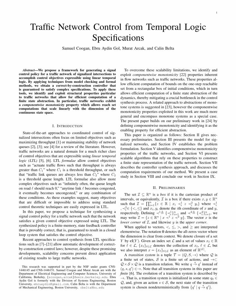
Fig. 6. Signalized network consisting of a major corridor road (links 1, 2, 3,and 4) which intersects minor cross streets (links 5, 6, 7, 8, 9, and 10). Thegray links are not explicitly modeled.

sums, operations that scale exponentially in |L| [36], [37]. Todetermine if Post(Iq, s) intersects another polytope, geomet-ric differences are required, which again scales exponentiallywith |L|.

VIII. CASE STUDY

We consider the example network in Fig. 6 whichconsists of a main corridor (links 1, 2, 3, and 4)with intersecting cross streets (links 5, 6, 7, 8, 9, and10) and four intersections, a commonly encountered net-work configuration. The gray links exit the networkand are not explicitly modeled. The network parametersare (xcap

1 , . . . , xcap10 ) = (40, 50, 50, 50, 40, 40, 40, 40, 40, 40),

(c1, . . . , c10) = (20, 20, 20, 20, 10, 10, 10, 10, 10, 10), β12 =β23 = β34 = β62 = β52 = 0.5, β73 = β84 = 0.9,α{1}62 = α

{1}52 = 0.5, and all other supply ratios are one, where

the time step is 15 seconds. We assume

D ={d | 0 ≤ d ≤ [10 0 0 0 10 10 0 0 10 10]}∪ {d | 0 ≤ d ≤ [10 0 0 0 10 10 10 10 0 0]}. (38)

We further assume the available signals are Sv1 ={{1}, {5, 6}}, Sv2 = {{2}, {7}}, Sv3 = {{3}, {8}}, andSv4 = {{4}, {9, 10}}. We wish to find a control policy forthe four signalized intersections that satisfies the LTL propertyϕ = ϕ1 ∧ ϕ2 ∧ ϕ3 ∧ ϕ4 where

ϕ1 =�♦(sv1 = {5, 6}) ∧�♦(sv2 = {7})∧�♦(sv3 = {8}) ∧�♦(sv4 = {9, 10}) (39)

“Each signal actuates cross street traffic infinitely often”

ϕ2 =♦�((x1 ≤ 30) ∧ (x2 ≤ 30) ∧ (x3 ≤ 30) ∧ (x4 ≤ 30)

)(40)

“Eventually, links 1, 2, 3, and 4 have fewer than 30vehicles on each link and this remains true for all time”

ϕ3 =�(¬(sv4 = {4}) ∧#(sv4 = {4})→##(sv4 = {4})

)(41)

ϕ4 =�(¬(sv4 = {9, 10}) ∧#(sv4 = {9, 10})

→##(sv4 = {9, 10}))

(42)For ϕ3 (resp. ϕ4), “The signal at intersection v4 mustactuate corridor traffic (resp. cross street traffic) for atleast two sequential time-steps.”

Thus, ϕ2 reflects our preference for actuating corridor trafficand ensures that eventually, links 2, 3, and 4 have “adequatesupply” because if the number of vehicles on these links is lessthan 30, then these links can always accept upstream demand,thus avoiding congestion (congestion occurs when demand isgreater than supply). Condition ϕ1 ensures that, despite the

9

0 5 10 15 20 25 30 350

10

20

30

40

50

60

70

Num

ber

ofV

ehic

les

onL

ink

Link 1Link 2

Link 3Link 4

0 5 10 15 20 25 30 35

Time Period

1234

Sign

al

(a)

0 5 10 15 20 25 30 350

10

20

30

40

50

60

70

Num

ber

ofV

ehic

les

onL

ink

Link 1Link 2

Link 3Link 4

0 5 10 15 20 25 30 35

Time Period

1234

Sign

al

(b)Fig. 7. (a) A sample trajectory of a naıve strategy that alternately actuatescorridor traffic and then cross street traffic for four time steps each ina synchronized fashion. This policy does not satisfy the desired controlobjective, in particular, (40) is not satisfied. (b) A sample trajectory resultingfrom the synthesized control policy that is guaranteed to satisfy the LTL policy(39)–(42). In the lower plots of (a) and (b), green (resp., red) for the signaltrace indicates corridor traffic (resp., cross street traffic) is actuated.

preference for facilitating traffic along the corridor, we mustinfinitely often actuate traffic at the cross streets. Conditionsϕ3 and ϕ4 are needed if, e.g. there exists crosswalks atintersection v4 and a minimum amount of time is requiredto allow pedestrians to cross. Note that repeated applicationof the # (“next”) operator allows us to consider finite timehorizons as in (41) and (42).

We partition the state space into 408 boxes that favors largerboxes when there are fewer total vehicles in the network. Thereare 16 signaling inputs, and thus, the number of states in thetransition system Taug is |Q| = 6528. The Rabin automatongenerated from ϕ contains 62 states and one acceptance pair.Computing the finite state abstraction T took 22.4 seconds.In contrast, the computation would be intractable using poly-hedral methods. Computing the product automaton took 30.9minutes and computing the control strategy took 15.5 minuteson a Macbook Pro with a 2.3 GHz processor where we usethe Rabin game solver in conPAS2 [14], however conPAS2is written in MATLAB and the synthesis process is likelyto be much more efficient if implemented in C or C++ andoptimized. Furthermore, all computations can be performedoffline and some are parallelizable, such as computing theproduct automaton. Finally, we note that the computed controlstrategy is implemented with minimal online costs.

Fig. 7(a) shows a sample trajectory of the network using a

naıve coordinated signaling strategy whereby each intersectionactuates corridor traffic for three time steps and then crosstraffic for three time steps. The exogenous disturbance isgenerated uniformly randomly from D. The trajectories arenot guaranteed to satisfy the control objective, in particular,ϕ2 is violated. Fig. 7(b) shows a sample trajectory of thesystem with a control strategy synthesized using the finite stateabstraction augmented with signal history and the LTL require-ment above. The control strategy is correct-by-constructionand thus guaranteed to satisfy ϕ from any initial state.

We see that the synthesized controller reacts to increasedvehicles on the corridor by actuating the corridor links, therebypreventing congestion (inadequate supply) along the corridor.At the same time, the controller actuates cross streets whendoing so does not adversely affect conditions on the corridor(i.e., cause congestion). In contrast, the fixed time controllerin Fig 7(a) is not able to react to the current conditions of thenetwork and fails to prevent congestion along the corridor; infact, links 2, 3, and 4 periodically reach full capacity.

IX. CONCLUSIONS

We have proposed a framework for synthesizing a controlstrategy for a traffic network that ensures the resulting trafficdynamics satisfy a control objective expressed in linear tem-poral logic (LTL). In addition to offering a novel domain forapplying formal methods tools in a control theory setting, wehave identified and exploited key properties of traffic networksto allow efficient computation of a finite state abstraction.

Future research will investigate systematic methods fordetermining an appropriate box partition to further reduce thenumber of states in the computed abstraction. Additionally,traffic networks are often composed of tightly coupled neigh-borhoods and towns connected by sparse longer roads, andsuch networks may be amenable to a compositional formalmethods approach using an assume-guarantee framework [5].

REFERENCES

[1] T. Wongpiromsarn, T. Uthaicharoenpong, Y. Wang, E. Frazzoli, andD. Wang, “Distributed traffic signal control for maximum networkthroughput,” in Intelligent Transportation Systems (ITSC), 2012 15thInternational IEEE Conference on, pp. 588–595, Sept 2012.

[2] P. Varaiya, “The max-pressure controller for arbitrary networks ofsignalized intersections,” in Advances in Dynamic Network Modelingin Complex Transportation Systems, pp. 27–66, Springer, 2013.

[3] P. Varaiya, “Max pressure control of a network of signalized intersec-tions,” Transportation Research Part C: Emerging Technologies, vol. 36,pp. 177–195, 2013.

[4] M. Papageorgiou, C. Diakaki, V. Dinopoulou, A. Kotsialos, and Y. Wang,“Review of road traffic control strategies,” Proceedings of the IEEE,vol. 91, no. 12, pp. 2043–2067, 2003.

[5] E. M. Clarke, O. Grumberg, and D. A. Peled, Model checking. MITpress, 1999.

[6] C. Baier and J. Katoen, Principals of Model Checking. MIT Press, 2008.[7] P. Tabuada and G. Pappas, “Linear time logic control of discrete-

time linear systems,” IEEE Transactions on Automatic Control, vol. 51,no. 12, pp. 1862–1877, 2006.

[8] P. Tabuada, “Controller synthesis for bisimulation equivalence,” Systems& Control Letters, vol. 57, no. 6, pp. 443–452, 2008.

[9] G. E. Fainekos, A. Girard, H. Kress-Gazit, and G. J. Pappas, “Temporallogic motion planning for dynamic robots,” Automatica, vol. 45, no. 2,pp. 343–352, 2009.

[10] H. Kress-Gazit, G. Fainekos, and G. Pappas, “Temporal-logic-basedreactive mission and motion planning,” IEEE Transactions on Robotics,vol. 25, pp. 1370–1381, Dec 2009.

10

[11] M. Kloetzer and C. Belta, “Automatic deployment of distributed teamsof robots from temporal logic motion specifications,” IEEE Transactionson Robotics, vol. 26, pp. 48–61, Feb 2010.

[12] A. Abate, A. D’Innocenzo, and M. Di Benedetto, “Approximate abstrac-tions of stochastic hybrid systems,” IEEE Transactions on AutomaticControl, vol. 56, pp. 2688–2694, Nov 2011.

[13] T. Wongpiromsarn, U. Topcu, and R. Murray, “Receding horizon tem-poral logic planning,” IEEE Transactions on Automatic Control, vol. 57,pp. 2817–2830, Nov 2012.

[14] B. Yordanov, J. Tumova, I. Cerna, J. Barnat, and C. Belta, “Temporallogic control of discrete-time piecewise affine systems,” IEEE Transac-tions on Automatic Control, vol. 57, no. 6, pp. 1491–1504, 2012.

[15] E. A. Gol, M. Lazar, and C. Belta, “Language-guided controller synthe-sis for linear systems,” IEEE Transactions on Automatic Control, vol. 59,pp. 1163–1176, May 2014.

[16] A. A. Julius and A. K. Winn, “Safety controller synthesis using humangenerated trajectories: Nonlinear dynamics with feedback linearizationand differential flatness,” in Proceedings of the 2012 American ControlConference, pp. 709–714, 2012.

[17] U. Topcu, N. Ozay, J. Liu, and R. M. Murray, “On synthesizing robustdiscrete controllers under modeling uncertainty,” in Proceedings of the15th ACM International Conference on Hybrid Systems: Computationand Control, HSCC ’12, (New York, NY, USA), pp. 85–94, ACM, 2012.

[18] J. Liu, N. Ozay, U. Topcu, and R. Murray, “Synthesis of reactive switch-ing protocols from temporal logic specifications,” IEEE Transactions onAutomatic Control, vol. 58, pp. 1771–1785, July 2013.

[19] E. Aydin Gol, M. Lazar, and C. Belta, “Temporal logic model pre-dictive control for discrete-time systems,” in Proceedings of the 16thInternational Conference on Hybrid Systems: Computation and Control,pp. 343–352, ACM, 2013.

[20] E. Plaku, L. E. Kavraki, and M. Y. Vardi, “Falsification of LTL safetyproperties in hybrid systems,” International Journal on Software Toolsfor Technology Transfer, vol. 15, no. 4, pp. 305–320, 2013.

[21] S. Coogan and M. Arcak, “Freeway traffic control from linear temporallogic specifications,” in Proceedings of the 5th ACM/IEEE InternationalConference on Cyber-Physical Systems, pp. 36–47, 2014.

[22] M. Kulenovic and O. Merino, “A global attractivity result for maps withinvariant boxes,” Discrete and Continuous Dynamical Systems Series B,vol. 6, no. 1, p. 97, 2006.

[23] T. Moor and J. Raisch, “Abstraction based supervisory controller synthe-sis for high order monotone continuous systems,” in Modelling, Analysis,and Design of Hybrid Systems, pp. 247–265, Springer, 2002.

[24] S. Coogan, E. Aydin Gol, M. Arcak, and C. Belta, “Controlling anetwork of signalized intersections from temporal logical specifications,”in American Control Conference (ACC), 2015. To appear.

[25] J. Lebacque, “Intersection modeling, application to macroscopic networktraffic flow models and traffic management,” in Traffic and GranularFlow’03, pp. 261–278, Springer, 2005.

[26] C. F. Daganzo, “The cell transmission model: A dynamic representationof highway traffic consistent with the hydrodynamic theory,” Transporta-tion Research Part B: Methodological, vol. 28, no. 4, pp. 269–287, 1994.

[27] J. C. Munoz and C. F. Daganzo, “The bottleneck mechanism of afreeway diverge,” Transportation Research Part A: Policy and Practice,vol. 36, no. 6, pp. 483–505, 2002.

[28] M. Kieffer, L. Jaulin, and E. Walter, “Guaranteed recursive non-linearstate bounding using interval analysis,” International Journal of AdaptiveControl and Signal Processing, vol. 16, no. 3, pp. 193–218, 2002.

[29] M. Papageorgiou, “An integrated control approach for traffic corridors,”Transportation Research Part C: Emerging Technologies, vol. 3, no. 1,pp. 19–30, 1995.

[30] F. H. Clarke, Optimization and nonsmooth analysis, vol. 5. Siam, 1990.[31] M. W. Hirsch, “Systems of differential equations that are competitive

or cooperative II: Convergence almost everywhere,” SIAM Journal onMathematical Analysis, vol. 16, no. 3, pp. 423–439, 1985.

[32] D. Angeli and E. Sontag, “Monotone control systems,” IEEE Transac-tions on Automatic Control, vol. 48, no. 10, pp. 1684–1698, 2003.

[33] H. L. Smith, Monotone dynamical systems: An introduction to the theoryof competitive and cooperative systems. American Math. Soc., 1995.

[34] S. Scholtes, Introduction to piecewise differentiable equations. Springer,2012.

[35] F. Horn, “Streett games on finite graphs,” Proc. 2nd Workshop Gamesin Design Verification (GDV), 2005.

[36] A. Kurzhanskiy and P. Varaiya, “Computation of reach sets for dynam-ical systems,” in The Control Systems Handbook, ch. 29, CRC Press,second ed., 2010.

[37] M. Herceg, M. Kvasnica, C. Jones, and M. Morari, “Multi-Parametric Toolbox 3.0,” in Proceedings of the European ControlConference, (Zurich, Switzerland), pp. 502–510, July 17–19 2013.http://control.ee.ethz.ch/∼mpt.

Samuel Coogan is a Ph.D. candidate in ElectricalEngineering and Computer Sciences at the Univer-sity of California, Berkeley. He received his B.S. inElectrical Engineering from Georgia Tech in 2010and his M.S. in Electrical Engineering from UCBerkeley in 2012. His research interests are in con-trol theory, nonlinear and hybrid systems, and formalmethods. He is particularly interested in applyingtechniques from these domains to the control anddesign of transportation systems. He received anNSF Graduate Research Fellowship in 2010 and the

Leon O. Chua Award for outstanding achievement in nonlinear science fromUC Berkeley in 2014.

Ebru Aydin Gol received her B.Sc. degree incomputer engineering from Orta Dogu Teknik Uni-versitesi, Ankara, Turkey, in 2008, M.Sc. degree incomputer science from Ecole Polytechnique Fed-erale de Lausanne, Lausanne, Switzerland, in 2010and Ph.D. degree in systems engineering fromBoston University, Boston, MA, USA in 2014. Shehas been a Site Reliability Engineer at Google since2014. Her research interests include verification andcontrol of dynamical systems, optimal control, andsynthetic biology.

Murat Arcak is a professor at U.C. Berkeley in theElectrical Engineering and Computer Sciences De-partment. He received the B.S. degree in ElectricalEngineering from the Bogazici University, Istanbul,Turkey (1996) and the M.S. and Ph.D. degrees fromthe University of California, Santa Barbara (1997and 2000). His research is in dynamical systems andcontrol theory with applications to synthetic biology,multi-agent systems, and transportation. Prior tojoining Berkeley in 2008, he was a faculty memberat the Rensselaer Polytechnic Institute. He received

a CAREER Award from the National Science Foundation in 2003, the DonaldP. Eckman Award from the American Automatic Control Council in 2006, theControl and Systems Theory Prize from the Society for Industrial and AppliedMathematics (SIAM) in 2007, and the Antonio Ruberti Young ResearcherPrize from the IEEE Control Systems Society in 2014. He is a member ofSIAM and a fellow of IEEE.

Calin Belta is a Professor in the Department ofMechanical Engineering, Department of Electricaland Computer Engineering, and the Division ofSystems Engineering at Boston University, where heis also affiliated with the Center for Information andSystems Engineering (CISE) and the BioinformaticsProgram. His research focuses on dynamics andcontrol theory, with particular emphasis on hybridand cyber-physical systems, formal synthesis andverification, and applications in robotics and systemsbiology. Calin Belta is a Senior Member of the IEEE

and an Associate Editor for the SIAM Journal on Control and Optimization(SICON) and the IEEE Transactions on Automatic Control. He received theAir Force Office of Scientific Research Young Investigator Award and theNational Science Foundation CAREER Award.