The Temporal Logic of Actions - lamport.azurewebsites.net · The temporal logic of actions (TLA) is a logic for specifying and reasoning about concurrent systems. Systems and their

The Temporal Logic of Actions

LESLIE LAMPORT

Digital Equipment Corporation

The temporal logic of actions (TLA) is a logic for specifying and reasoning about concurrentsystems. Systems and their properties are represented in the same logic, so the assertion thata system meets its specification and the assertion that one system implements another are bothexpressed by logical implication. TLA is very simple; its syntax and complete formal semantics aresummarized in about a page. Yet, TLA is not just a logician’s toy; it is extremely powerful, bothin principle and in practice. This report introduces TLA and describes how it is used to specifyand verify concurrent algorithms. The use of TLA to specify and reason about open systems willbe described elsewhere.

Categories and Subject Descriptors: D.2.4 [Software Engineering]: Program Verification—correctness proofs; F.3.1 [Logics and Meanings of Programs]: Specifying and Verifying andReasoning about Programs—Specification techniques

General terms: Theory, Verification

Additional Key Words and Phrases: Concurrent programming, liveness properties, safety proper-ties

1. LOGIC VERSUS PROGRAMMING

A concurrent algorithm is usually specified with a program. Correctness of thealgorithmmeans that the program satisfies a desired property. We propose a simplerapproach in which both the algorithm and the property are specified by formulas ina single logic. Correctness of the algorithm means that the formula specifying thealgorithm implies the formula specifying the property, where implies is ordinarylogical implication.

We are motivated not by an abstract ideal of elegance, but by the practicalproblem of reasoning about real algorithms. Rigorous reasoning is the only wayto avoid subtle errors in concurrent algorithms, and we want to make reasoning assimple as possible by making the underlying formalism simple.

How can we abandon conventional programming languages in favor of logic if thealgorithmmust be coded as a program to be executed? The answer is that we almostalways reason about an abstract algorithm, not about a concurrent program thatis actually executed. A typical example is the distributed spanning-tree algorithmused in the Autonet local area network [Schroeder et al. 1990]. The algorithm canbe described in about one page of pseudo-code, but its implementation required

Author’s address: Systems Research Center, Digital Equipment Corporation, 130 Lytton Avenue,Palo Alto, CA 94301.Permission to copy without fee all or part of this material is granted provided that the copies are

not made or distributed for direct commercial advantage, the ACM copyright notice and the titleof the publication and its date appear, and notice is given that copying is by permission of theAssociation for Computing Machinery. To copy otherwise, or to republish, requires a fee and/orspecific permission.c© 1993 ACM 0000-0000/93/0000-0000 $00.00

ACM Transactions on Programming Languages and Systems, Vol ? No. ?, November 1993, Pages 1–52.

2 · Leslie Lamport

about 5000 lines of C code and 500 lines of assembly code.1 Reasoning about5000 lines of C would be a herculean task, but we can reason about a one-pageabstract algorithm. By starting from a correct algorithm, we can avoid the timing-dependent synchronization errors that are the bane of concurrent programming. Ifthe algorithms we reason about are not real, compilable programs, then they donot have to be written in a programming language.

But, why replace a programming language by logic? Aren’t programs simplerthan logical formulas? The answer is no. Logic is the formalization of everydaymathematics, and everyday mathematics is simpler than programs. Consider thePascal statement y := x + 1. Using the convention that y′ denotes the new valueof y, we can rewrite this statement as the mathematical formula y′ = x+ 1. Manyreaders will think that the Pascal statement and the formula are equally simple.They are wrong. The formula is much simpler than the Pascal statement. Equalityis a simple concept that five-year-old children understand. Assignment (:=) is acomplicated concept that university students find difficult. Equality obeys simplealgebraic laws; assignment doesn’t. If we assume that all variables are integer-valued, we can subtract y′ from both sides of the formula to obtain the equivalentformula 0 = x+ 1− y′. Trying this with the Pascal statement yields the absurdity0 := x+ 1− y.

A programming language may use mathematical terms like function, but the con-structs they represent are not as simple as the corresponding mathematical con-cepts. Mathematical functions are simple; children in the United States learn aboutthem at the age of twelve. Pascal functions are complicated, involving concepts likecall by reference, call by value, and aliasing; it is unlikely that many universitystudents understand them well. Advocates of so-called functional programminglanguages often claim that they just use ordinary mathematical functions, but tryexplaining to a twelve-year-old how evaluating a mathematical function can displaya character on her computer screen.

Since real languages like Pascal are so complicated, methods for reasoning aboutalgorithms are usually based on toy languages. Although simpler than real pro-gramming languages, toy languages are more complicated than simple logic. More-over, their resemblance to real languages can be dangerously misleading. In toylanguages, the Hoare triple {x = 0} y := x + 1 {y = x + 1} is valid, which meansthat executing y := x + 1 in a state in which x equals 0 produces a state in whichy equals x+ 1. However, in Pascal, the program fragment

x := 0; y := x+ 1; write(y, x+ 1)

can print two different values when used in certain contexts, even if x and y arevariables of type integer. The programmer who tries using toy-language rules toreason about real Pascal programs is in for a rude surprise.

We do not mean to belittle programming languages. They are complicated be-cause they have a difficult job to do. Mathematics can be based on simple conceptslike functions. Programming languages cannot, because they must allow reason-ably simple compilers to translate programs into reasonably efficient code for com-plex computers. Real languages must embrace difficult concepts like the distinc-tion between values and locations, which leads to call-by-reference arguments and

1Assembly code was needed because C has no primitives for sending messages across wires.

ACM Transactions on Programming Languages and Systems, Vol ?, No. ?, November 1993.

The Temporal Logic of Actions · 3

aliasing—complications that have no counterpart in simple mathematics. Program-ming languages are necessary for writing real programs; but mathematics offers asimpler alternative for reasoning about concurrent algorithms.

To offer a practical alternative to programming languages, a logic must be bothsimple and expressive. There is no point trading a programming language for alogic that is just as complicated and hard to understand. Furthermore, a logicthat achieves simplicity at the expense of needed expressiveness will be impracticalbecause the formulas describing real algorithms will be too long and complicatedto understand.

The logic that we propose for reasoning about concurrent algorithms is the tem-poral logic of actions, abbreviated as TLA. All TLA formulas can be expressed interms of familiar mathematical operators (such as ∧) plus three new ones: ′ (prime),✷, and ∃∃∃∃∃∃. TLA is simple enough that its syntax and complete formal semantics canbe written in about a page. Almost all that is needed to specify and reason aboutalgorithms in TLA—its syntax, formal semantics, derived notation, and axioms andproof rules—appears in Figures 4 and 5 of Section 5.6 and Figure 9 of Section 8.2.(Missing from those figures are the rules for adding auxiliary variables, mentionedin Section 8.3.2.)

Logic is a tool. Its true test comes with use. Although TLA and its proof rulescan be described formally in a couple of pages, such a description would tell younothing about how TLA is used. In this article, we develop TLA as a method ofdescribing and reasoning about concurrent algorithms. We limit ourselves to simpleexamples, so we can only hint at how TLA works with real algorithms.

TLA combines two logics: a logic of actions, described in Section 2, and a stan-dard temporal logic, described in Section 3. TLA is easiest to explain in terms of alogic called RTLA, which is defined in Section 4. We describe TLA itself and illus-trate its use in Sections 5–8. Section 9 mentions further applications and discusseswhat TLA can and cannot do, and Section 10 relates TLA to other formalisms.

2. THE LOGIC OF ACTIONS

2.1 Values, Variables, and States

Algorithms manipulate data. We assume a collection Val of values, where a value isa data item. The collection Val includes numbers such as 1, 7, and −14, strings like“abc”, and sets like the set Nat of natural numbers. We don’t bother to define Valprecisely, but simply assume that it contains all the values needed for our examples(Note2 1). We also assume the booleans true and false, which for technical reasonsare not considered to be values.

We think of algorithms as assigning values to variables. We assume an infinite setVar of variable names. We won’t describe a precise syntax for generating variablenames, but will simply use names like x and sem.

A logic consists of a set of rules for manipulating formulas. To understand whatthe formulas and their manipulation mean, we need a semantics. A semantics isgiven by assigning a semantic meaning [[F ]] to each syntactic object F in the logic.

The semantics of our logic is defined in terms of states. A state is an assignmentof values to variables—that is, a mapping from the set Var of variable names to

2Notes appear at the end of the article.


4 · Leslie Lamport

the collection Val of values. Thus a state s assigns a value s(x) to a variable x. Thecollection of all possible states is denoted St.

We write s[[x]] to denote s(x). Thus, we consider the meaning [[x]] of the variablex to be a mapping from states to values, using a postfix notation for functionapplication. States and values are purely semantic concepts; they do not appearexplicitly in formulas.

2.2 State Functions and Predicates

A state function is a nonboolean expression built from variables and constantsymbols—for example, x2+y−3 (Note 2). The meaning [[f ]] of a state function f isa mapping from the collection St of states to the collection Val of values. For exam-ple, [[x2 +y−3]] is the mapping that assigns to a state s the value (s[[x]])2 +s[[y]]−3,where 2 and 3 are constant symbols, and 2 and 3 are the values that they represent.We will not bother distinguishing between constant symbols and their values. Weuse a postfix functional notation, letting s[[f ]] denote the value that [[f ]] assigns tostate s. The semantic definition is

s[[f ]] ∆= f(∀ ‘v ’ : s[[v]]/v) (1)

where f(∀ ‘v ’ : s[[v]]/v) denotes the value obtained from f by substituting s[[v]] forv, for all variables v. (The symbol ∆= means equals by definition.)

A variable x is a state function—the state function that assigns the value s[[x]]to the state s. The definition of [[f ]] for a state function f therefore extends thedefinition of [[x]] for a variable x.

A state predicate, called a predicate for short, is a boolean expression built fromvariables and constant symbols—for example, x2 = y−3 and x ∈ Nat. The meaning[[P ]] of a predicate P is a mapping from states to booleans, so s[[P ]] equals true orfalse for every state s. We say that a state s satisfies a predicate P iff (if and onlyif) s[[P ]] equals true.

State functions correspond both to expressions in ordinary programming lan-guages and to subexpressions of the assertions used in ordinary program verifica-tion. Predicates correspond both to boolean-valued expressions in programminglanguages and to assertions.

2.3 Actions

An action is a boolean-valued expression formed from variables, primed variables,and constant symbols—for example, x′ + 1 = y and x − 1 /∈ z′ are actions, wherex, y, and z are variables.

An action represents a relation between old states and new states, where theunprimed variables refer to the old state and the primed variables refer to the newstate. Thus, y = x′ + 1 is the relation asserting that the value of y in the oldstate is one greater than the value of x in the new state. An atomic operation of aconcurrent program will be represented in TLA by an action.

Formally, the meaning [[A]] of an actionA is a relation between states—a functionthat assigns a boolean s[[A]]t to a pair of states s, t. We define s[[A]]t by considerings to be the “old state” and t the “new state”, so s[[A]]t is obtained from A byreplacing each unprimed variable v by s[[v]] and each primed variable v′ by t[[v]]:

s[[A]]t ∆= A(∀ ‘v ’ : s[[v]]/v, t[[v]]/v′) (2)



Thus, s[[y = x′ + 1]]t equals the boolean s[[y]] = t[[x]] + 1.The pair of states s, t is called an “A step” iff s[[A]]t equals true. If action A

represents an atomic operation of a program, then s, t is an A step iff executing theoperation in state s can produce state t.

2.4 Predicates as Actions

We have defined a predicate P to be a boolean-valued expression built from variablesand constant symbols, so s[[P ]] is a boolean, for any state s. We can also view Pas an action that contains no primed variables. Thus, s[[P ]]t is a boolean, whichequals s[[P ]], for any states s and t. A pair of states s, t is a P step iff s satisfies P .

Both state functions and predicates are expressions built from variables and con-stant symbols. For any state function or predicate F , we define F ′ to be theexpression obtained by replacing each variable v in F by the primed variable v′:

F ′ ∆= F (∀ ‘v ’ : v′/v) (3)

If P is a predicate, then P ′ is an action, and s[[P ′]]t equals t[[P ]] for any states sand t.

2.5 Validity and Provability

An action A is said to be valid, written |= A, iff every step is an A step. Formally,

|= A ∆= ∀s, t ∈ St : s[[A]]t

As a special case of this definition, if P is a predicate, then

|= P ∆= ∀s ∈ St : s[[P ]]

A valid action is one that is true regardless of what values one substitutes for theprimed and unprimed variables. For example, the action

(x′ + y ∈ Nat) ⇒ (2(x′ + y) ≥ x′ + y) (4)

is valid. The validity of an action thus expresses a theorem about values.A logic contains rules for proving formulas. It is customary to write F to

denote that formula F is provable by the rules of the logic. Soundness of the logicmeans that every provable formula is valid—in other words, that F implies |= F .The validity of an action such as (4) is proved by ordinary mathematical reasoning(Note 3). How this reasoning is formalized does not concern us here, so we willnot bother to define a logic for proving the validity of actions. But, this omissiondoes not mean such reasoning is unimportant. When verifying the validity of TLAformulas, most of the work goes into proving the validity of actions (and of predi-cates, a special class of actions). The practical success of any TLA verification willdepend primarily on how good the verifier is at ordinary mathematical reasoning.

2.6 Rigid Variables and Quantifiers

Consider a program that is described in terms of a parameter n—for example, ann-process mutual exclusion algorithm. An action representing an atomic operationof that programmay contain the symbol n. This symbol does not represent a knownvalue like 1 or “abc”. But unlike the variables we have considered so far, the valueof n does not change; it must be the same in the old and new state.


6 · Leslie Lamport

The symbol n denotes some fixed but unknown value. A programmer would callit a constant because its value doesn’t change during execution of the program,while a mathematician would call it a variable because it is an “unknown”. Wecall such a symbol n a rigid variable. The variables introduced above will be calledflexible variables, or simply variables.

An expression like n+1, built from rigid variables and constant symbols, is calleda constant expression. We generalize state functions and actions to allow arbitraryconstant expressions instead of just constant symbols, and to allow quantificationover rigid variables. For example, if x is a (flexible) variable and m and n are rigidvariables, then ∃m ∈ Nat : mx′ = n + x is the action asserting that there existssome natural number m such that m times the value of x in the new state equals nplus its value in the old state (Note 4):

s [[∃m ∈ Nat : mx′ = n + x]] t ∆= ∃m ∈ Nat : m(t[[x]]) = n + s[[x]]

Thus, the semantics of state functions and actions is no longer given in termsonly of values, but of first-order formulas containing free rigid variables and values.However, a state is still an assignment of values to flexible variables.

An action A is valid iff s[[A]]t equals true for all states s and t and all possiblevalues of its free rigid variables—for example:

|= (x′ + y + m ∈ Nat) ⇒ ∀n ∈ Nat : n(x′ + y + m) ≥ (x′ + y + m)

We do not permit quantification over flexible variables in state functions and ac-tions.

2.7 The Enabled Predicate

For any action A, we define Enabled A to be the predicate that is true for a stateiff it is possible to take an A step starting in that state. Semantically, Enabled Ais defined by

s[[Enabled A]] ∆= ∃ t ∈ St : s[[A]]t (5)

for any state s. The predicate Enabled A can be defined syntactically as follows.If v1, . . . , vn are all the (flexible) variables that occur in A, then

Enabled A ∆= ∃ c1, . . . , cn : A(c1/v′1, . . . , cn/v

′n)

where A(c1/v′1, . . . , cn/v

′n) denotes the formula obtained by substituting new rigid

variables ci for all occurrences of the v′i in A. For example,

Enabled (y = (x′)2 + n) ≡ ∃ c : y = c2 + n

If action A represents an atomic operation of a program, then Enabled A is truefor those states in which it is possible to perform the operation.

3. SIMPLE TEMPORAL LOGIC

An execution of an algorithm is often thought of as a sequence of steps, eachproducing a new state by changing the values of one or more variables. We willconsider an execution to be the resulting sequence of states, and will take thesemantic meaning of an algorithm to be the collection of all its possible executions.Reasoning about algorithms will therefore require reasoning about sequences ofstates. Such reasoning is the province of temporal logic.ACM Transactions on Programming Languages and Systems, Vol ?, No. ?, November 1993.


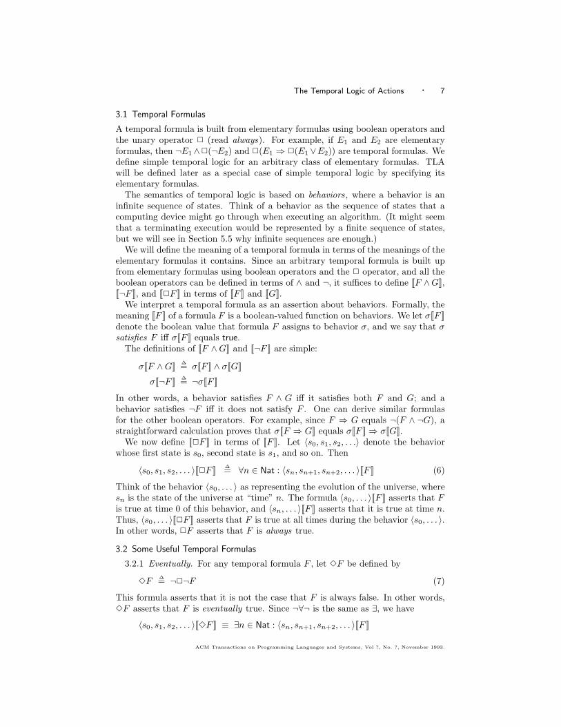
3.1 Temporal Formulas

A temporal formula is built from elementary formulas using boolean operators andthe unary operator ✷ (read always). For example, if E1 and E2 are elementaryformulas, then ¬E1 ∧✷(¬E2) and ✷(E1 ⇒ ✷(E1 ∨E2)) are temporal formulas. Wedefine simple temporal logic for an arbitrary class of elementary formulas. TLAwill be defined later as a special case of simple temporal logic by specifying itselementary formulas.

The semantics of temporal logic is based on behaviors , where a behavior is aninfinite sequence of states. Think of a behavior as the sequence of states that acomputing device might go through when executing an algorithm. (It might seemthat a terminating execution would be represented by a finite sequence of states,but we will see in Section 5.5 why infinite sequences are enough.)

We will define the meaning of a temporal formula in terms of the meanings of theelementary formulas it contains. Since an arbitrary temporal formula is built upfrom elementary formulas using boolean operators and the ✷ operator, and all theboolean operators can be defined in terms of ∧ and ¬, it suffices to define [[F ∧G]],[[¬F ]], and [[✷F ]] in terms of [[F ]] and [[G]].

We interpret a temporal formula as an assertion about behaviors. Formally, themeaning [[F ]] of a formula F is a boolean-valued function on behaviors. We let σ[[F ]]denote the boolean value that formula F assigns to behavior σ, and we say that σsatisfies F iff σ[[F ]] equals true.

The definitions of [[F ∧G]] and [[¬F ]] are simple:

σ[[F ∧G]] ∆= σ[[F ]] ∧ σ[[G]]σ[[¬F ]] ∆= ¬σ[[F ]]

In other words, a behavior satisfies F ∧ G iff it satisfies both F and G; and abehavior satisfies ¬F iff it does not satisfy F . One can derive similar formulasfor the other boolean operators. For example, since F ⇒ G equals ¬(F ∧ ¬G), astraightforward calculation proves that σ[[F ⇒ G]] equals σ[[F ]] ⇒ σ[[G]].

We now define [[✷F ]] in terms of [[F ]]. Let 〈s0, s1, s2, . . .〉 denote the behaviorwhose first state is s0, second state is s1, and so on. Then

〈s0, s1, s2, . . . 〉[[✷F ]] ∆= ∀n ∈ Nat : 〈sn, sn+1, sn+2, . . . 〉[[F ]] (6)

Think of the behavior 〈s0, . . . 〉 as representing the evolution of the universe, wheresn is the state of the universe at “time” n. The formula 〈s0, . . . 〉[[F ]] asserts that Fis true at time 0 of this behavior, and 〈sn, . . . 〉[[F ]] asserts that it is true at time n.Thus, 〈s0, . . . 〉[[✷F ]] asserts that F is true at all times during the behavior 〈s0, . . . 〉.In other words, ✷F asserts that F is always true.

3.2 Some Useful Temporal Formulas

3.2.1 Eventually. For any temporal formula F , let ✸F be defined by

✸F∆= ¬✷¬F (7)

This formula asserts that it is not the case that F is always false. In other words,✸F asserts that F is eventually true. Since ¬∀¬ is the same as ∃, we have

〈s0, s1, s2, . . . 〉[[✸F ]] ≡ ∃n ∈ Nat : 〈sn, sn+1, sn+2, . . . 〉[[F ]]


8 · Leslie Lamport

for any behavior 〈s0, s1, . . . 〉. Therefore, a behavior satisfies ✸F iff F is true atsome time during the behavior.

3.2.2 Infinitely Often and Eventually Always. The formula ✷✸F is true for abehavior iff ✸F is true at all times n during that behavior, and ✸F is true at timen iff F is true at some time m greater than or equal to n. Formally,

〈s0, s1, . . . 〉[[✷✸F ]] ≡ ∀n ∈ Nat : ∃m ∈ Nat : 〈sn+m, sn+m+1, . . . 〉[[F ]]

A formula of the form ∀n : ∃m : g(n + m) asserts that g(i) is true for infinitelymany values of i. Thus, a behavior satisfies ✷✸F iff F is true at infinitely manytimes during the behavior. In other words, ✷✸F asserts that F is true infinitelyoften.

The formula ✸✷F asserts that eventually F is always true. Thus, a behaviorsatisfies ✸✷F iff there is some time such that F is true from that time on.

3.2.3 Leads To. For any temporal formulas F and G, we define F ❀ G to equal✷(F ⇒ ✸G). This formula asserts that any time F is true, G is true then or atsome later time. The operator ❀ (read leads to) is transitive, meaning that anybehavior satisfying F ❀ G and G ❀ H also satisfies F ❀ H . We suggest thatreaders convince themselves both that ❀ is transitive, and that it would not behad F ❀ G been defined to equal F ⇒ ✸G.

3.3 Validity and Provability

A temporal formula F is said to be valid, written |= F , iff it is satisfied by allpossible behaviors. More precisely,

|= F ∆= ∀σ ∈ St∞ : σ[[F ]] (8)

where St∞ denotes the collection of all behaviors (infinite sequences of elements ofSt).

We will represent both algorithms and properties as temporal formulas. Analgorithm is represented by a temporal formula F such that σ[[F ]] equals true iff σrepresents a possible execution of the algorithm. If G is a temporal formula, thenF ⇒ G is valid iff σ[[F ⇒ G]] equals true for every behavior σ. Since σ[[F ⇒ G]]equals σ[[F ]] ⇒ σ[[G]], validity of F ⇒ G means that every behavior representing apossible execution of the algorithm satisfies G. In other words, |= F ⇒ G assertsthat the algorithm represented by F satisfies property G.

In Section 5.6, we give rules for proving temporal formulas. As usual, soundnessof the rules means that every provable formula is valid—that is, F implies |= Ffor any temporal formula F .

4. THE RAW LOGIC

4.1 Actions as Temporal Formulas

The Raw Temporal Logic of Actions, or RTLA, is obtained by letting the elementarytemporal formulas be actions. To define the semantics of RTLA formulas, we mustdefine what it means for an action to be true on a behavior.

In Section 2.3, we defined the meaning [[A]] of an action A to be a boolean-valuedfunction that assigns the value s[[A]]t to the pair of states s, t. We defined s, t to be



an A step iff s[[A]]t equals true. We now define [[A]] to be true for a behavior iff thefirst pair of states in the behavior is an A step (Note 5). Formally,

〈s0, s1, s2, . . . 〉[[A]] ∆= s0[[A]]s1 (9)

RTLA formulas are built up from actions using logical operators and the temporaloperator ✷. Thus, if A is an action, then ✷A is an RTLA formula. Its meaning iscomputed as follows.

〈s0, s1, s2, . . . 〉[[✷A]]≡ ∀n ∈ Nat : 〈sn, sn+1, sn+2, . . . 〉[[A]] by (6)≡ ∀n ∈ Nat : sn[[A]]sn+1 by (9)

In other words, a behavior satisfies ✷A iff every step of the behavior is an A step.In Section 2.4, we observed that if P is a predicate, then s[[P ]]t equals s[[P ]].

Therefore,

〈s0, s1, . . . 〉[[P ]] ≡ s0[[P ]]〈s0, s1, . . . 〉[[✷P ]] ≡ ∀n ∈ Nat : sn[[P ]]

In other words, a behavior satisfies a predicate P iff the first state of the behaviorsatisfies P . A behavior satisfies ✷P iff all states in the behavior satisfy P .

We will see that the raw logic RTLA is too powerful; it allows one to make as-sertions about behaviors that should not be assertable. We will define the formulasof TLA to be a subset of RTLA formulas.

4.2 Describing Programs with RTLA Formulas

We have defined the syntax and semantics of RTLA formulas, but have given noidea what RTLA is good for. We illustrate how RTLA can be used, by describingthe simple Program 1 of Figure 1 as an RTLA formula. This program is written ina conventional language, using Dijkstra’s do construct [Dijkstra 1976], with anglebrackets enclosing operations that are assumed to be atomic. An execution of thisprogram begins with x and y both zero, and repeatedly increments either x or y (ina single operation), choosing nondeterministically between them. We now definean RTLA formula Φ that represents this program, meaning that σ[[Φ]] equals trueiff the behavior σ represents a possible execution of Program 1.

The formula Φ is defined in Figure 2. The predicate InitΦ asserts the initialcondition, that x and y are both zero. The semantic meaning of action M1 is arelation between states asserting that the value of x in the new state is one greaterthan its value in the old state, and the value of y is the same in the old and newstates. Thus, anM1 step represents an execution of the program’s atomic operationof incrementing x. Similarly, an M2 step represents an execution of the program’sother atomic operation, which increments y. The action M is defined to be thedisjunction of M1 and M2, so an M step represents an execution of one programoperation. Formula Φ is true of a behavior iff InitΦ is true of the first state andevery step is an M step. In other words, Φ asserts that the initial condition is true

var natural x, y = 0 ;do 〈 true → x := x + 1 〉

〈 true → y := y + 1 〉 od

Fig. 1. Program 1—a simple program, written in aconventional language.


10 · Leslie Lamport

InitΦ∆= (x = 0) ∧ (y = 0)

M1∆= (x′ = x + 1) ∧ (y′ = y) M2

∆= (y′ = y + 1) ∧ (x′ = x)

M ∆= M1 ∨M2

Φ∆= InitΦ ∧ ✷M

Fig. 2. An RTLA formula Φ describing Program 1.

initially, and that every step of the behavior represents the execution of an atomicoperation of the program. Clearly, a behavior satisfies Φ iff it represents a possibleexecution of Program 1 (Note 6).

There is nothing special about our choice of names, or in the particular way ofwriting Φ. There are many ways of writing equivalent logical formulas. Here are acouple of formulas that are equivalent to Φ.

(x = 0) ∧ ✷(M1 ∨M2) ∧ (y = 0)InitΦ ∧ ✷((x′ = x+ 1) ∨ (y′ = y + 1)) ∧ ✷((x′ = x) ∨ (y′ = y))

The particular way of defining Φ in Figure 2 was chosen to make the correspondencewith Figure 1 obvious.

5. TLA

5.1 Adding Stuttering Steps

Formula Φ of Figure 2 is very simple. Unfortunately, it is too simple. In additionto steps in which x or y is incremented, a formula describing Program 1 shouldallow “stuttering” steps that leave both x and y unchanged.

To understand why stuttering steps are needed, consider a clock that displayshours and minutes. It is specified by a formula Π with two variables: h representingthe hours display and m representing the minutes display. Now consider a clockthat displays hours, minutes, and seconds; it is represented by a formula Ψ withthree variables: h, m, and another variable s representing the seconds display. Aclock that displays hours, minutes, and seconds should satisfy the specification Πof a clock that displays hours and minutes. (If we don’t want the seconds display,we can always cover it up.) Hence, any behavior satisfying Ψ should satisfy Π.Behaviors satisfying Ψ contain sequences of 59 consecutive steps in which h andm do not change, so Π must allow such steps. From the point of view of a clockdisplaying only hours and minutes, steps in which h and m do not change arestuttering steps. In general, a specification Π should be invariant under stuttering,meaning that adding or removing stuttering steps from a behavior does not affectwhether the behavior satisfies Π.

It is easy to modify formula Φ of Figure 2 so it asserts that every step is eitheran M step or a step that leaves x and y unchanged; the new definition is

Φ ∆= InitΦ ∧ ✷(M ∨ ((x′ = x) ∧ (y′ = y))) (10)

We now introduce notation that makes it easy to ensure that a formula allowsstuttering steps. Two ordered pairs are equal iff their components are equal, so theconjunction (x′ = x)∧ (y′ = y) is equivalent to the single equality 〈x′, y′〉 = 〈x, y〉.The definition of priming a state function (formula (3)) allows us to write 〈x′, y′〉



as 〈x, y〉′ (Note 7). For any action A and state function f , we let

[A]f∆= A ∨ (f ′ = f) (11)

(The action [A]f is read square A sub f .) Then

[M]〈x, y〉 ≡ M ∨ (〈x, y〉′ = 〈x, y〉)≡ M ∨ ((x′ = x) ∧ (y′ = y))

and we can rewrite (10) as

Φ ∆= InitΦ ∧ ✷[M]〈x, y〉 (12)

We define TLA to be the temporal logic whose elementary formulas are predicatesand formulas of the form ✷[A]f , where A is an action and f a state function.Since these formulas are RTLA formulas, we have already defined their semanticmeanings.

5.2 Adding Liveness

The formula Φ defined by (12) allows behaviors that start with InitΦ true (x andy both zero) and never change x or y. Such behaviors do not represent acceptableexecutions of Program 1, so we must strengthen Φ to disallow them.

Formula Φ of (12) asserts that a behavior may not start in any state other thanone satisfying InitΦ and may never take any step other than a [M]〈x, y〉 step. Anassertion that something may never happen is called a safety property. An assertionthat something eventually does happen is called a liveness property. (Safety andliveness have been defined formally by Alpern and Schneider [1985].) The formulaInitΦ ∧ ✷[M]〈x, y〉 is a safety property. To complete the description of Program 1,we need an additional liveness property asserting that the program keeps going.

By Dijkstra’s semantics for his do construct, the liveness property for Program 1should assert only that the program never terminates. In other words, Dijkstrawould require that a behavior must contain infinitely many steps that increment xor y. This property is expressed by the RTLA formula ✷✸M, which asserts thatthere are infinitely many M steps. Dijkstra would have us define Φ by

Φ ∆= InitΦ ∧ ✷[M]〈x, y〉 ∧ ✷✸M (13)

However, the example becomes more interesting if we add the fairness requirementthat both x and y must be incremented infinitely often. (Dijkstra’s definition wouldallow an execution in which one variable is incremented infinitely often while theother is incremented only a finite number of times.) Since we are not fettered bythe dictates of conventional programming languages, we will adopt this strongerliveness requirement. The formula Φ representing the program with this fairnessrequirement is

Φ ∆= InitΦ ∧ ✷[M]〈x, y〉 ∧ ✷✸M1 ∧ ✷✸M2 (14)

Formulas (13) and (14) are RTLA formulas, but not TLA formulas. An action Acan appear in a TLA formula only in the form ✷[A]f (unless A is a predicate), so✷✸M1 and ✷✸M2 are not TLA formulas. We now rewrite them as TLA formulas.

Let A be any action and f any state function. Then ¬A is also an action, so¬✷[¬A]f is a TLA formula. Applying our definitions gives



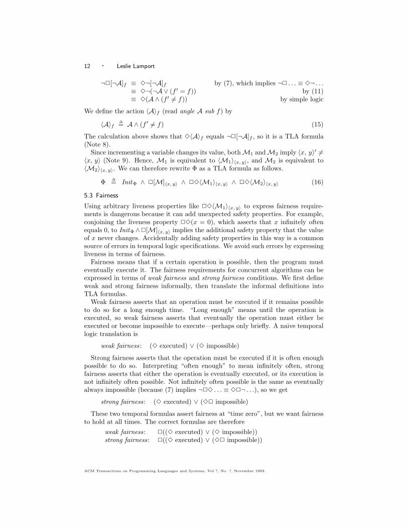
¬✷[¬A]f ≡ ✸¬[¬A]f by (7), which implies ¬✷ . . . ≡ ✸¬ . . .≡ ✸¬(¬A ∨ (f ′ = f)) by (11)≡ ✸(A ∧ (f ′ �= f)) by simple logic

We define the action 〈A〉f (read angle A sub f) by

〈A〉f ∆= A ∧ (f ′ �= f) (15)

The calculation above shows that ✸〈A〉f equals ¬✷[¬A]f , so it is a TLA formula(Note 8).

Since incrementing a variable changes its value, both M1 andM2 imply 〈x, y〉′ �=〈x, y〉 (Note 9). Hence, M1 is equivalent to 〈M1〉〈x, y〉, and M2 is equivalent to〈M2〉〈x, y〉. We can therefore rewrite Φ as a TLA formula as follows.

Φ ∆= InitΦ ∧ ✷[M]〈x, y〉 ∧ ✷✸〈M1〉〈x, y〉 ∧ ✷✸〈M2〉〈x, y〉 (16)

5.3 Fairness

Using arbitrary liveness properties like ✷✸〈M1〉〈x, y〉 to express fairness require-ments is dangerous because it can add unexpected safety properties. For example,conjoining the liveness property ✷✸(x = 0), which asserts that x infinitely oftenequals 0, to InitΦ ∧✷[M]〈x, y〉 implies the additional safety property that the valueof x never changes. Accidentally adding safety properties in this way is a commonsource of errors in temporal logic specifications. We avoid such errors by expressingliveness in terms of fairness.

Fairness means that if a certain operation is possible, then the program musteventually execute it. The fairness requirements for concurrent algorithms can beexpressed in terms of weak fairness and strong fairness conditions. We first defineweak and strong fairness informally, then translate the informal definitions intoTLA formulas.

Weak fairness asserts that an operation must be executed if it remains possibleto do so for a long enough time. “Long enough” means until the operation isexecuted, so weak fairness asserts that eventually the operation must either beexecuted or become impossible to execute—perhaps only briefly. A naive temporallogic translation is

weak fairness : (✸ executed) ∨ (✸ impossible)

Strong fairness asserts that the operation must be executed if it is often enoughpossible to do so. Interpreting “often enough” to mean infinitely often, strongfairness asserts that either the operation is eventually executed, or its execution isnot infinitely often possible. Not infinitely often possible is the same as eventuallyalways impossible (because (7) implies ¬✷✸ . . . ≡ ✸✷¬ . . .), so we get

strong fairness : (✸ executed) ∨ (✸✷ impossible)

These two temporal formulas assert fairness at “time zero”, but we want fairnessto hold at all times. The correct formulas are therefore

weak fairness : ✷((✸ executed) ∨ (✸ impossible))strong fairness : ✷((✸ executed) ∨ (✸✷ impossible))



Temporal logic reasoning, using either the axioms in Section 5.6 or the semanticdefinitions of ✷ and ✸, shows that these conditions are equivalent to

weak fairness : (✷✸ executed) ∨ (✷✸ impossible)strong fairness : (✷✸ executed) ∨ (✸✷ impossible)

To formalize these definitions, we must define “executed” and “impossible”.In Program 1, execution of the operation x := x+ 1 corresponds to an M1 step

in the behavior. To obtain a TLA formula, the “✸ executed” for this operationmust be expressed as ✸〈M1〉〈x, y〉. In general, “✸ executed” will be expressed as✸〈A〉f , where A is the action that corresponds to an execution of the operation,and f is an n-tuple of relevant variables. Recall that an 〈A〉f step is an A stepthat changes the value of f . Steps that do not change the values of any relevantvariables might as well not have occurred, so there is no need to consider them asrepresenting operation executions.

We now define “impossible”. Executing an operation means taking an 〈A〉fstep for some action A and state function f . It is possible to take such a step iffEnabled 〈A〉f is true. Thus, Enabled 〈A〉f asserts that it is possible to execute theoperation represented by the action 〈A〉f , so “impossible” is ¬Enabled 〈A〉f . Weakfairness and strong fairness are therefore expressed by the two formulas

WFf (A) ∆= (✷✸〈A〉f ) ∨ (✷✸¬Enabled 〈A〉f ) (17)

SFf (A) ∆= (✷✸〈A〉f ) ∨ (✸✷¬Enabled 〈A〉f ) (18)

Since ✸✷F implies ✷✸F for any F , the strong fairness condition SFf (A) impliesthe weak fairness condition WFf (A).

The pair of formulas Init ∧✷[N ]v , F is said to be machine closed if conjoining Fto Init ∧ ✷[N ]v introduces no additional safety properties. (In this case, we oftensay that Init ∧ ✷[N ]v ∧ F is machine closed.) We avoid accidentally adding safetyproperties by writing machine-closed specifications. It can be shown that if F isthe conjunction of fairness conditions of the form WFf (A) and/or SFf (A), whereeach 〈A〉f implies N , then Init ∧✷[N ]v ∧F is machine closed [Abadi and Lamport1992].

5.4 Rewriting the Fairness Requirement

We now rewrite the property ✷✸〈M1〉〈x, y〉 ∧ ✷✸〈M2〉〈x, y〉 in terms of fairnessconditions. An 〈M1〉〈x, y〉 step is one that increments x by one, leaves y un-changed, and changes the value of 〈x, y〉. It is always possible to take a stepthat adds one to x and leaves y unchanged, and adding one to a number changesit. Hence, Enabled 〈M1〉〈x, y〉 equals true throughout any execution of Program 1(Note 10). Since ✷¬true equals false, both WF〈x, y〉(M1) and SF〈x, y〉(M1) equal✷✸〈M1〉〈x, y〉. Similarly, WF〈x, y〉(M2) and SF〈x, y〉(M2) both equal ✷✸〈M2〉〈x, y〉.We can therefore rewrite the definition (16) of Φ as shown in Figure 3.

Suppose we wanted the weaker liveness condition that execution never termi-nates, so the program is described by the RTLA formula (13). The same argu-ment as for M1 and M2 shows that ✷✸〈M〉〈x, y〉 equals WF〈x, y〉(M). Therefore,Program 1 with this weaker liveness condition is described by the TLA formulaInitΦ ∧ ✷[M]〈x, y〉 ∧ WF〈x, y〉(M).

The actions 〈M1〉〈x, y〉, 〈M2〉〈x, y〉, and 〈M〉〈x, y〉 all imply M. Hence neither ofthe liveness conditions WF〈x, y〉(M1)∧WF〈x, y〉(M2) and WF〈x, y〉(M1) add safety



properties to InitΦ ∧ ✷[M]〈x, y〉.

5.5 Examining Formula Φ

TLA formulas that represent programs can always be written in the same form asΦ of Figure 3—that is, as a conjunction Init ∧ ✷[N ]f ∧ F , where

Init is a predicate specifying the initial values of variables.N is the program’s next-state relation, the action whose steps represent execu-

tions of individual atomic operations.f is the n-tuple of all flexible variables.F is the conjunction of formulas of the form WFf (A) and/or SFf (A), where A

is an action representing some subset of the program’s atomic operations.

We now examine the behaviors that satisfy formula Φ. Let

((x ∆= 7, y ∆= −10, z ∆= “abc”, . . . ))

denote a state s such that s[[x]] = 7, s[[y]] = −10, and s[[z]] = “abc”. (The “. . .”indicates that the value of s[[v]] is left unspecified for all other variables v.) Abehavior that satisfies Φ begins in a state satisfying InitΦ, and consists of a sequenceof [M]〈x, y〉 steps—ones that are either M steps or else leave x and y unchanged.One such behavior is

(( x ∆= 0, y ∆= 0, z ∆= “abc” . . . ))(( x ∆= 1, y ∆= 0, z ∆= 14 . . . ))(( x ∆= 2, y ∆= 0, z ∆= Nat . . . ))(( x ∆= 2, y ∆= 0, z ∆= −20 . . . ))(( x ∆= 2, y ∆= 1, z ∆=

√2 . . . ))

...

Observe that Φ constrains only the values of x and y; it allows all other variablessuch as z to assume completely arbitrary values. Suppose Ψ is a formula describinga program that has no variables in common with Φ. Then a behavior satisfies Φ∧Ψiff it represents an execution of both programs—that is, iff it describes a universein which both Φ and Ψ are executed concurrently. Thus, Φ∧Ψ is the TLA formularepresenting the parallel composition of the two programs.

In general, parallel composition is represented in TLA by conjunction. For ex-ample, let

Φ1∆= (x = 0) ∧ ✷[M1]x ∧ WFx(M1)

Φ2∆= (y = 0) ∧ ✷[M2]y ∧ WFy(M2)

InitΦ∆= (x = 0) ∧ (y = 0)

M1∆= (x′ = x + 1) ∧ (y′ = y) M2

∆= (y′ = y + 1) ∧ (x′ = x)

M ∆= M1 ∨M2

Φ∆= InitΦ ∧ ✷[M]〈x, y〉 ∧ WF〈x, y〉(M1) ∧ WF〈x, y〉(M2)

Fig. 3. The TLA formula Φ describing Program 1.



A straightforward calculation shows that [M1]x ∧ [M2]y is equivalent to [M]〈x, y〉,and temporal logic reasoning (using the axioms of Section 5.6) then shows that Φ isequivalent to Φ1∧Φ2. Formulas Φ1 and Φ2 are the specifications of the two processesforming Program 1. This example illustrates a general method for decomposing thespecification of a multiprocess program as the conjunction of the specifications ofits processes [Abadi and Lamport 1993].

The observation that a single behavior can represent an execution of two ormore noninteracting programs explains why we represent terminating as well asnonterminating executions by infinite behaviors. Termination of a program meansthat it has stopped; it does not mean that the entire universe has come to a halt.A terminating execution is represented by a behavior in which eventually all of theprogram’s variables stop changing.

It is unusual in computer science for the semantics of a formula describing aprogram with variables x and y to involve other variables such as z that appearnowhere in the program. One of the keys to TLA’s simplicity is that its semanticsrests on a single, infinite set of variables—not on a different set of variables for eachprogram. Thus, in TLA as in elementary logic, we can take the conjunction F ∧Gof any formulas F and G—not just of formulas with properly matching variabledeclarations.

5.6 Simple TLA

We now complete the definition of Simple TLA by adding one more bit of nota-tion. (The full logic, containing quantification, is introduced in Section 8.) It isconvenient to define the action Unchanged f , for f a state function, by

Unchanged f ∆= f ′ = f

Thus, an Unchanged f step is one in which the value of f does not change.The syntax and semantics of Simple TLA, along with the additional notation we

use to write TLA formulas, are all summarized in Figure 4. This figure explains allyou need to know to understand TLA formulas such as formula Φ of Figure 3.

A logic contains not only syntax and semantics, but also rules for proving theo-rems. Figure 5 lists all the axioms and proof rules we need for proving simple TLAformulas.3

The rules of simple temporal logic are used to derive temporal tautologies—formulas that are true regardless of the meanings of their elementary formulas.Rule STL1 encompasses the rules of ordinary logic, such as modus ponens (Note 11).The Lattice Rule assumes a (possibly infinite) set S and a mapping that assigns aTLA formula Hc to each element c of S. A partial order � on S is well-foundediff there exists no infinite descending chain c1 � c2 � . . . with all the ci in S.This rule permits the formalization of counting-down arguments, such as the onestraditionally used to prove termination of sequential programs.

Rules STL1–STL6, the Lattice Rule, and the basic rules TLA1 and TLA2 form arelatively complete proof system for reasoning about algorithms in TLA. Roughlyspeaking, this means that every valid TLA formula that we must prove to verifyproperties of algorithms would be provable from these rules if we could prove all

3A proof rule F, GH

asserts that � F and � G imply � H. We use the term “rule” for both axioms

and proof rules, since an axiom may be viewed as a proof rule with no hypotheses.



Syntax

〈formula〉 ∆= 〈predicate〉 | ✷[〈action〉]〈state function〉 | ¬〈formula〉

| 〈formula〉 ∧ 〈formula〉 | ✷ 〈formula〉〈action〉 ∆

= boolean-valued expression containing constant symbols,variables, and primed variables

〈predicate〉 ∆= 〈action〉 with no primed variables | Enabled 〈action〉

〈state function〉 ∆= nonboolean expression containing constant symbols and variables

Semantics

s[[f ]]∆= f(∀ ‘v ’ : s[[v]]/v) σ[[F ∧ G]]

∆= σ[[F ]] ∧ σ[[G]]

s[[A]]t∆= A(∀ ‘v ’ : s[[v]]/v, t[[v]]/v′) σ[[¬F ]]

∆= ¬σ[[F ]]

|= A ∆= ∀s, t ∈ St : s[[A]]t |= F

∆= ∀σ ∈ St∞ : σ[[F ]]

s[[Enabled A]]∆= ∃t ∈ St : s[[A]]t

〈s0, s1, . . . 〉[[✷F ]]∆= ∀n ∈ Nat : 〈sn, sn+1, . . . 〉[[F ]]

〈s0, s1, . . . 〉[[A]]∆= s0[[A]]s1

Additional notation

p′ ∆= p(∀ ‘v ’ : v′/v) ✸F

∆= ¬✷¬F

[A]f∆= A ∨ (f ′ = f) F ❀ G

∆= ✷(F ⇒ ✸G)

〈A〉f ∆= A ∧ (f ′ �= f) WFf (A)

∆= ✷✸〈A〉f ∨ ✷✸¬Enabled 〈A〉f

Unchanged f∆= f ′ = f SFf (A)

∆= ✷✸〈A〉f ∨ ✸✷¬Enabled 〈A〉f

where f is a 〈state function〉 s, s0, s1, . . . are states

A is an 〈action〉 σ is a behavior

F and G are 〈formula〉s (∀ ‘v ’ : . . . /v, . . . /v′) denotes substitution

p is a 〈state function〉 or 〈predicate〉 for all variables v

Fig. 4. Simple TLA.

valid action formulas. (This is analogous to the traditional relative completenessresults for program verification, which assume provability of all valid predicates [Apt1981].) A more precise statement of this result is given in Section 8.3.2 below(Note 12).

A complete proof system is not necessarily a convenient one. For practical rea-soning, STL1–STL6 should be augmented with some useful temporal tautologieslike

(✷F ) ∧ (✸G) ⇒ ✸(F ∧G)

With practice, such simple tautologies become as obvious as the ordinary laws ofpropositional logic. They are usually taken for granted in hand proofs, and practicaldecision procedures exist for checking them mechanically [Burch et al. 1992]. Thetemporal operators ✷, ✸, and ❀ are standard [Manna and Pnueli 1991], so we willnot discuss the rules of simple temporal logic.

Assuming simple temporal reasoning, we have found that TLA2 and the “addi-tional rules” INV1–SF2 of Figure 5 provide a convenient system for all the proofsthat arise in reasoning about programs with TLA. The overbars in rules WF2 andSF2 are explained in Section 8.3.3; for now, the reader can pretend that they arenot there, obtaining special cases of the rules.



The Rules of Simple Temporal Logic

STL1. F provable bypropositional logic

✷F

STL4. F ⇒ G

✷F ⇒ ✷G

STL2. � ✷F ⇒ F STL5. � ✷(F ∧ G) ≡ (✷F ) ∧ (✷G)

STL3. � ✷✷F ≡ ✷F STL6. � (✸✷F ) ∧ (✸✷G) ≡ ✸✷(F ∧ G)

LATTICE. � a well-founded partial order on a set SF ∧ (c ∈ S) ⇒ (Hc ❀ (G ∨ ∃d ∈ S : (c � d) ∧ Hd))

F ⇒ ((∃c ∈ S : Hc) ❀ G)

The Basic Rules of TLA

TLA1. P ∧ (f ′ = f) ⇒ P ′

✷P ≡ P ∧ ✷[P ⇒ P ′]f

TLA2. P ∧ [A]f ⇒ Q ∧ [B]g

✷P ∧ ✷[A]f ⇒ ✷Q ∧ ✷[B]g

Additional Rules

INV1. I ∧ [N ]f ⇒ I′

I ∧ ✷[N ]f ⇒ ✷I

INV2. � ✷I ⇒ (✷[N ]f ≡ ✷[N ∧ I ∧ I′]f )

WF1.P ∧ [N ]f ⇒ (P ′ ∨ Q′)P ∧ 〈N ∧ A〉f ⇒ Q′P ⇒ Enabled 〈A〉f

✷[N ]f ∧WFf (A) ⇒ (P ❀ Q)

WF2.

〈N ∧ B〉f ⇒ 〈M〉gP ∧ P ′ ∧ 〈N ∧ A〉f ∧ Enabled 〈M〉g ⇒ BP ∧ Enabled 〈M〉g ⇒ Enabled 〈A〉f✷[N ∧ ¬B]f ∧WFf (A) ∧ ✷F

∧ ✸✷Enabled 〈M〉g ⇒ ✸✷P

✷[N ]f ∧WFf (A) ∧ ✷F ⇒ WFg(M)

SF1.P ∧ [N ]f ⇒ (P ′ ∨ Q′)P ∧ 〈N ∧ A〉f ⇒ Q′✷P ∧ ✷[N ]f ∧ ✷F ⇒ ✸Enabled 〈A〉f✷[N ]f ∧ SFf (A) ∧ ✷F ⇒ (P ❀ Q)

SF2.

〈N ∧ B〉f ⇒ 〈M〉gP ∧ P ′ ∧ 〈N ∧ A〉f ⇒ BP ∧ Enabled 〈M〉g ⇒ Enabled 〈A〉f✷[N ∧ ¬B]f ∧ SFf (A) ∧ ✷F

∧ ✷✸Enabled 〈M〉g ⇒ ✸✷P

✷[N ]f ∧ SFf (A) ∧ ✷F ⇒ SFg(M)

where F , G, Hc are TLA formulas P , Q, I are predicatesA, B, N , M are actions f , g are state functions

Fig. 5. The axioms and proof rules of Simple TLA.



The validity of these rules can be proved rigorously with the raw logic RTLA.Rules STL1–STL6 are valid when F and G are arbitrary RTLA formulas, not justTLA formulas. The validity of TLA1–SF2 can be proved using STL1–STL6 andthe RTLA rule ✷P ≡ P ∧ ✷(P ⇒ P ′). The validity of this rule follows easily fromthe semantic definitions of ✷ and ′ (prime). We leave the rigorous proofs as anexercise for the reader; instead, we give informal justifications. Sections 6 and 7illustrate how the rules are used.

Rule TLA1 provides an induction principle for proving the formula ✷P . It assertsthe obvious fact that a predicate P is always true iff P holds initially and everystep starting with P true leaves P true.

Rule TLA2 follows immediately from the validity of STL4 and STL5 for RTLAformulas. (We have to use RTLA because ✷(P ∧ [A]f ) is not a TLA formula.)

Rule INV1 is used to prove that a program satisfies an invariance property ✷I.The hypothesis asserts that a [N ]f step cannot falsify I. The conclusion asserts theobvious consequence that if I is true initially and every step is a [N ]f step, then Iis always true.

Rule WF1 is used to deduce a leads-to property P ❀ Q from a weak fairnesscondition WFf (A). It can be applied when an A step that starts with P truemakes Q true. To prove the validity of the conclusion, we assume that every stepis a [N ]f step and that WFf (A) holds, and we prove P ❀ Q. It suffices to derivea contradiction by assuming that P is true at some time n and Q is false then andat all later times. Since every step is a [N ]f step and Q is false from time n on,the first hypothesis implies that P is true from time n on. The third hypothesisthen implies that Enabled 〈A〉f is true from time n on. Hence, WFf (A) impliesthat infinitely many A steps occur. Any such step occurring after time n startswith P true, and the second hypothesis implies that the step makes Q true. Thiscontradicts the assumption that Q remains false after time n, proving the validityof the rule.

Rule WF2 is used to deduce one weak fairness condition from another. We deduceWFg(M) from WFf (A) by finding an action B such that every B step is an Mstep and, if M remains forever enabled, then eventually every A step is a B step.(We ignore the overbars.) To prove the validity of WF2, we first observe that sinceWFg(M) equals ✷✸¬Enabled 〈M〉g ∨✷✸〈M〉g and ✸ equals ¬✷¬, we can rewritethe conclusion as follows.

✷[N ]f ∧WFf (A) ∧ ✷F ∧ ✸✷Enabled 〈M〉g ⇒ ✷✸〈M〉gIt therefore suffices to obtain a contradiction by assuming that ✷[N ]f ∧WFf (A)∧✷F∧✸✷Enabled 〈M〉g holds and only finitely many 〈M〉g steps occur. Since [N ]f∧〈B〉f equals 〈N ∧ B〉f , it follows from the first hypothesis that only finitely many〈B〉f steps can occur. Hence, there must eventually be a time after which no more〈B〉f steps occur, so every further step is a [N∧¬B]f step. By the fourth hypothesis,there must then be a time at which P becomes true forever. The third hypothesisthen implies that Enabled 〈A〉f eventually becomes true forever, so WFf (A) impliesthat there are infinitely many 〈A〉f steps. The second hypothesis then implies thatthere are infinitely many 〈B〉f steps, which is the required contradiction.

Rules SF1 and SF2 are the analogs of WF1 and WF2 for strong fairness. Weomit their justifications, which are similar to those of WF1 and WF2.



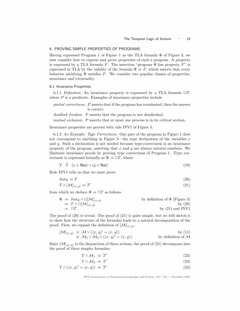
6. PROVING SIMPLE PROPERTIES OF PROGRAMS

Having expressed Program 1 of Figure 1 as the TLA formula Φ of Figure 3, wenow consider how to express and prove properties of such a program. A propertyis expressed by a TLA formula F . The assertion “program Φ has property F” isexpressed in TLA by the validity of the formula Φ ⇒ F , which asserts that everybehavior satisfying Φ satisfies F . We consider two popular classes of properties,invariance and eventuality.

6.1 Invariance Properties

6.1.1 Definition. An invariance property is expressed by a TLA formula ✷P ,where P is a predicate. Examples of invariance properties include

partial correctness. P asserts that if the program has terminated, then the answeris correct.

deadlock freedom. P asserts that the program is not deadlocked.mutual exclusion. P asserts that at most one process is in its critical section.

Invariance properties are proved with rule INV1 of Figure 5.

6.1.2 An Example: Type Correctness. One part of the program in Figure 1 doesnot correspond to anything in Figure 3—the type declaration of the variables xand y. Such a declaration is not needed because type-correctness is an invarianceproperty of the program, asserting that x and y are always natural numbers. Weillustrate invariance proofs by proving type correctness of Program 1. Type cor-rectness is expressed formally as Φ ⇒ ✷T , where

T∆= (x ∈ Nat) ∧ (y ∈ Nat) (19)

Rule INV1 tells us that we must prove

InitΦ ⇒ T (20)T ∧ [M]〈x, y〉 ⇒ T ′ (21)

from which we deduce Φ ⇒ ✷T as follows

Φ ⇒ InitΦ ∧ ✷[M]〈x, y〉 by definition of Φ (Figure 3)⇒ T ∧ ✷[M]〈x, y〉 by (20)⇒ ✷T by (21) and INV1

The proof of (20) is trivial. The proof of (21) is quite simple, but we will sketch itto show how the structure of the formulas leads to a natural decomposition of theproof. First, we expand the definition of [M]〈x, y〉.

[M]〈x, y〉 ≡ M∨ (〈x, y〉′ = 〈x, y〉) by (11)≡ M1 ∨M2 ∨ (〈x, y〉′ = 〈x, y〉) by definition of M

Since [M]〈x, y〉 is the disjunction of three actions, the proof of (21) decomposes intothe proof of three simpler formulas:

T ∧M1 ⇒ T ′ (22)T ∧M2 ⇒ T ′ (23)

T ∧ (〈x, y〉′ = 〈x, y〉) ⇒ T ′ (24)



We consider the proof of (22); the others are equally simple. First, we expand thedefinition of T ′.

T ′ ≡ ((x ∈ Nat) ∧ (y ∈ Nat))′ by (19)≡ (x′ ∈ Nat) ∧ (y′ ∈ Nat) by (3)

The structure of T ′ as the conjunction of two actions leads to the decomposition ofthe proof of (22) into the proof of the two simpler formulas

T ∧M1 ⇒ x′ ∈ Nat (25)T ∧M1 ⇒ y′ ∈ Nat (26)

The proof of (25) is

T ∧M1 ⇒ (x ∈ Nat) ∧ (x′ = x+ 1) by definition of T and M1

⇒ x′ ∈ Nat by properties of natural numbers

and the proof of (26) is equally trivial.The purpose of this exercise in simple mathematics is to illustrate how “mechan-

ical” the proof of this invariance property is. Rule INV1 tells us we must prove(20) and (21), and the structure of [M]〈x, y〉 and T leads to the decomposition ofthose proofs into the verification of simple facts about natural numbers, such as(x ∈ Nat) ⇒ (x + 1 ∈ Nat).

6.1.3 General Invariance Proofs. The proof of Φ ⇒ ✷T was simple because T isan invariant of the action [M]〈x, y〉, meaning that T ∧ [M]〈x, y〉 implies T ′. There-fore, Φ ⇒ ✷T could be proved by simply substituting T for I in rule INV1. Forinvariance properties ✷P other than simple type correctness, P is usually not aninvariant. In general, one proves that ✷P is an invariance property of the programrepresented by the TLA formula Init ∧ ✷[N ]f ∧ F by finding a predicate I (theinvariant) satisfying the three conditions

Init ⇒ I (27)I ⇒ P (28)I ∧ [N ]f ⇒ I ′ (29)

Rule INV1 and some simple temporal reasoning shows that (27)–(29) imply Init ∧✷[N ]f ⇒ ✷P .

Creative thought is needed to find the invariant I. Once I is found, verifying (27)–(29) is a matter of mechanically applying the definitions and using the structureof the formulas to decompose the proofs, just as in the proof of Φ ⇒ ✷T above.The formulas Init , I, and N will usually be much more complicated than in theexample, but the principle is the same.

Formulas (27)–(29) are assertions about predicates and actions; they are not tem-poral formulas. All the work in proving an invariance property is done in the realmof predicates and actions—expressions involving variables and primed variables thatcan be manipulated by ordinary mathematics. Temporal reasoning is used only todeduce Init ∧✷[N ]f ⇒ ✷P from (27)–(29). TLA is practical because it minimizestemporal reasoning, relying on ordinary, nontemporal reasoning whenever possible.

6.1.4 More About Invariance Proofs. Over the years, many methods have beenproposed for proving invariance properties of programs, including Floyd’s method



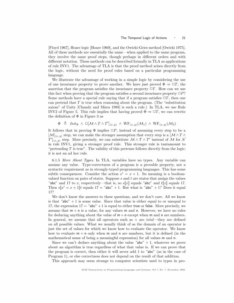
[Floyd 1967], Hoare logic [Hoare 1969], and the Owicki-Gries method [Owicki 1975].All of these methods are essentially the same—when applied to the same program,they involve the same proof steps, though perhaps in different orders and withdifferent notation. These methods can be described formally in TLA as applicationsof rule INV1. The advantage of TLA is that the proof method arises directly fromthe logic, without the need for proof rules based on a particular programminglanguage.

We illustrate the advantage of working in a simple logic by considering the useof one invariance property to prove another. We have just proved Φ ⇒ ✷T , theassertion that the program satisfies the invariance property ✷T . How can we usethis fact when proving that the program satisfies a second invariance property ✷P?Some methods have a special rule saying that if a program satisfies ✷T , then onecan pretend that T is true when reasoning about the program. (The “substitutionaxiom” of Unity [Chandy and Misra 1988] is such a rule.) In TLA, we use RuleINV2 of Figure 5. This rule implies that having proved Φ ⇒ ✷T , we can rewritethe definition of Φ in Figure 3 as

Φ ∆= InitΦ ∧ ✷[M∧ T ∧ T ′]〈x, y〉 ∧ WF〈x, y〉(M1) ∧ WF〈x, y〉(M2)

It follows that in proving Φ implies ✷P , instead of assuming every step to be a[M]〈x, y〉 step, we can make the stronger assumption that every step is a [M∧ T ∧T ′]〈x, y〉 step. More precisely, we can substitute M ∧ T ∧ T ′ instead of M for Nin rule INV1, giving a stronger proof rule. This stronger rule is tantamount to“pretending T is true”. The validity of this pretense follows directly from the logic;it is not an ad hoc rule.

6.1.5 More About Types. In TLA, variables have no types. Any variable canassume any value. Type-correctness of a program is a provable property, not asyntactic requirement as in strongly-typed programming languages. This has somesubtle consequences. Consider the action x′ = x + 1. Its meaning is a boolean-valued function on pairs of states. Suppose s and t are states that assign the values“abc” and 17 to x, respectively—that is, so s[[x]] equals “abc” and t[[x]] equals 17.Then s[[x′ = x + 1]]t equals 17 = “abc” + 1. But what is “abc” + 1? Does it equal17?

We don’t know the answers to these questions, and we don’t care. All we knowis that “abc” + 1 is some value. Since that value is either equal to or unequal to17, the expression 17 = “abc”+1 is equal to either true or false. More precisely, weassume that m + n is a value, for any values m and n. However, we have no rulesfor deducing anything about the value of m+ n except when m and n are numbers.In general, we assume that all operators such as + are total—they are definedon all possible values. What we usually think of as the domain of an operator isjust the set of values for which we know how to evaluate the operator. We knowhow to evaluate m + n only when m and n are numbers, but it is defined (in themathematical sense of being a meaningful expression) for all values m and n.

Since we can’t deduce anything about the value “abc” + 1, whatever we proveabout an algorithm is true regardless of what that value is. If we can prove thatthe program is correct, then either it will never add 1 to “abc” (as in the case ofProgram 1), or else correctness does not depend on the result of that addition.

This approach may seem strange to computer scientists used to types in pro-



gramming languages, but it captures the way mathematicians have reasoned forthousands of years. For example, mathematicians would say that the formula

(n ∈ Nat) ⇒ (n + 1 > n) (30)

is true for all n. Substituting “abc” for n yields

(“abc” ∈ Nat) ⇒ (“abc” + 1 > “abc”)

This formula is true regardless of what “abc” + 1 equals, and whether or not thatvalue is greater than “abc”, because “abc” ∈ Nat is false (Note 13). The formulais not meaningless or “type-incorrect” just because we don’t know the value of“abc” + 1.

There is one subtle pitfall raised by the absence of types in TLA. It is tempting tothink that we can replace x′ = x+1 by x = x′−1 in the TLA formula Φ describingProgram 1. However, these two expressions need not be equivalent unless x and x′

are both numbers. For example, if x equals 16, then x′ = x + 1 is true only if x′

equals 17. However, we don’t know what “abc” − 1 equals, so it might equal 16.Hence, the formula 16 = x′ − 1 might be true when x′ equals “abc” as well as whenx′ equals 17. We could not prove the property Φ ⇒ ✷(x ∈ Nat) if we replacedx′ = x+ 1 by x = x′ − 1 in the definition of Φ.

We can avoid this pitfall by writing actions as conjunctions and disjunctions offormulas of the form v′ = e and v′ ∈ e, where v is a variable and e a state function.The absence of types then produces no surprises. Moreover, actions written in thisform have the advantage of being easier to understand, since they express the newvalues of variables directly in terms of their old values.

We could define a typed version of TLA. Semantically, we just restrict thecollection of states to ones that assign to each variable a value of the proper type.However, types add a great deal of complexity to a logic. For example, what isthe type of the division operator? If it is Real × NonzeroReal → Real , then typecorrectness becomes undecidable, so we lose automatic type checking, arguably themajor benefit of types. If the type is Real ×Real → Real , then what is the value of1/0? If it is a real number, then we will be able to prove the correctness of algorithmsthat we would usually consider to be incorrect, such as an iterative algorithm thattakes 1/0 as an initial approximation. Letting 1/0 be a special “undefined” value⊥ leads to a complicated logic with truth values true, false, and ⊥.

The type of an operator like division is just one of many problems introduced bytypes. These problems are easily hidden in informal presentation such as ours andthe ones in most articles and books—for example, [Manna and Pnueli 1991] and[Chandy and Misra 1988]. The problems cannot be avoided in a formal treatment,such as is necessary for true mechanical verification. (They can be hidden whenmechanically checking hand-translated verification conditions). Although one canformalize a typed version of TLA, the result is not nearly so simple as the untypedversion. Types may be good for programming languages, but we believe that thedifficulties they add far outweigh their advantages in a logic for reasoning aboutalgorithms (Note 14).

6.2 Eventuality Properties

The second class of properties we consider are eventuality properties—ones as-serting that something eventually happens. Here are some traditional eventuality



properties and their expressions in temporal logic:

termination. The program eventually terminates: ✸ terminated .service. If a process has requested service, then it eventually is served:

requested ❀ served .message delivery. If a message is sent often enough, then it is eventually

delivered: (✷✸ sent) ⇒ ✸ delivered .

Although eventuality properties are expressed by a variety of temporal formulas,their proofs can always be reduced to the proof of leads-to properties—formulas ofthe form P ❀ Q. For example, suppose we want to prove that Program 1 increasesthe value of x without bound. The TLA formula to be proved is

Φ ∧ (n ∈ Nat) ⇒ ✸(x > n) (31)

The Lattice Rule of Figure 5 together with some simple temporal reasoning showsthat (31) follows from

Φ ⇒ ((n ∈ Nat ∧ x = n) ❀ (x = n + 1)) (32)

To illustrate the use of TLA in proving leads-to properties, we now sketch the proofof (32).

Since safety properties don’t imply that anything ever happens, leads-to prop-erties must be derived from the program’s fairness condition. Examining Figure 5leads us to try rule WF1, with the following substitutions:

P ← n ∈ Nat ∧ x = n N ← M f ← 〈x, y〉Q← x = n + 1 A ← M1

The rule’s hypotheses become

(n ∈ Nat ∧ x = n) ∧ [M]〈x, y〉 ⇒ ((n ∈ Nat ∧ x′ = n) ∨ (x′ = n + 1))(n ∈ Nat ∧ x = n) ∧ 〈M1〉〈x, y〉 ⇒ (x′ = n + 1)(n ∈ Nat ∧ x = n) ⇒ Enabled 〈M1〉〈x, y〉

which follow easily from the definitions of M1 and M in Figure 3. The rule’sconclusion becomes

✷[M]〈x, y〉 ∧WF〈x, y〉(M1) ⇒ ((n ∈ Nat ∧ x = n) ❀ (x = n + 1))

which, by definition of Φ, implies (32).

6.3 Other Properties

We have seen how invariance properties and eventuality properties are expressedas TLA formulas and proved. But, what about more complicated properties? Howwould one state the following property as a TLA formula?

A behavior begins with x and y both zero, and repeatedly incrementseither x or y (in a single operation), choosing nondeterministically be-tween them, but choosing each infinitely many times.

The answer, of course, it that we already have expressed this property in TLA. Itis formula Φ of Figure 3.

In TLA, there is no distinction between a program and a property. Instead ofviewing Φ as a description of a program, we can just as well consider it to be a



var integer x, y = 0 ;semaphore sem = 1 ;

cobegin loop α1: 〈 P (sem) 〉 ;β1: 〈 x := x + 1 〉 ;γ1: 〈 V (sem) 〉 endloop

loop α2: 〈 P (sem) 〉 ;β2: 〈 y := y + 1 〉 ;γ2: 〈 V (sem) 〉 endloop

coend

Fig. 6. Program 2—our second example program.

property that we want a program to satisfy. The formula Φ, like the program ofFigure 1 that it represents, is so simple that we can regard it as a specification ofhow we want a program to behave. As our next example, we consider a programthat implements property Φ. That is, we give a program represented by a TLAformula Ψ that implies Φ.

7. ANOTHER EXAMPLE

7.1 Program 2

Our next example is Program 2 of Figure 6, written in a language invented forthis program. (Since its only purpose is to help us write the TLA formula, theprogramming-language description of the program can be written with any conve-nient notation.) The program consists of two processes, each repeatedly execut-ing a loop that contains three atomic operations. The variable sem is an integersemaphore, and P and V are the standard semaphore operations [Dijkstra 1968].Since Figure 6 is an informal description, it doesn’t matter whether or not youunderstand it. The real definition of Program 2 is the TLA formula Ψ definedbelow.

Describing the execution of Program 2 as a sequence of states requires each stateto specify not only the values of the variables x, y, and sem, but also the controlstate of each process. Control in process 1 can be at one of the three “controlpoints” α1, β1, or γ1. We introduce the variable pc1 that will assume the values“a”, “b”, and “g”, denoting that control is at α1, β1, and γ1, respectively. A similarvariable pc2 denotes the control state of process 2.

The definition of the TLA formula Ψ that represents Program 2 is given inFigure 7 .4 A vertically aligned list of formulas preceded by “∧”s or “∨”s denotes theconjunction or disjunction of those formulas, and we use indentation to eliminateparentheses. (These notational conventions make large formulas much easier toread.) Thus, Figure 7 defines the predicate InitΨ to be the conjunction of threeformulas, the second of which is (x = 0) ∧ (y = 0).

As we explained in Section 5.5, a program is represented by a formula Init ∧✷[N ]f ∧F . In this example, Init and f are fairly obvious: Init is the predicate InitΨ

that specifies the initial values of the variables, and f is the 5-tuple w consisting ofall the program’s variables. The next-state relation N and the fairness requirementF are less obvious and merit some discussion.

4Section 9.2 discusses why Figure 7 is longer and seems more complex than Figure 6.



InitΨ∆= ∧ (pc1 = “a”) ∧ (pc2 = “a”)

∧ (x = 0) ∧ (y = 0)∧ sem = 1

α1∆= ∧ (pc1 = “a”) ∧ (0 < sem)

∧ pc′1 = “b”∧ sem ′ = sem − 1∧ Unchanged 〈x, y, pc2〉

α2∆= ∧ (pc2 = “a”) ∧ (0 < sem)

∧ pc′2 = “b”∧ sem′ = sem − 1∧ Unchanged 〈x, y, pc1〉

β1∆= ∧ pc1 = “b”

∧ pc′1 = “g”∧ x′ = x + 1∧ Unchanged 〈y, sem, pc2〉

β2∆= ∧ pc2 = “b”

∧ pc′2 = “g”∧ y′ = y + 1∧ Unchanged 〈x, sem, pc1〉

γ1∆= ∧ pc1 = “g”

∧ pc′1 = “a”∧ sem ′ = sem + 1∧ Unchanged 〈x, y, pc2〉

γ2∆= ∧ pc′2 = “a”

∧ pc2 = “g”∧ sem ′ = sem + 1∧ Unchanged 〈x, y, pc1〉

N1∆= α1 ∨ β1 ∨ γ1 N2

∆= α2 ∨ β2 ∨ γ2

N ∆= N1 ∨ N2

w∆= 〈x, y, sem, pc1, pc2〉

Ψ∆= InitΨ ∧ ✷[N ]w ∧ SFw(N1) ∧ SFw(N2)

Fig. 7. The formula Ψ describing Program 2.

7.1.1 The Next-State Relation. Corresponding to the six atomic operations inFigure 6 are the six actions α1, . . . , γ2 defined in Figure 7. The four conjuncts inthe definition of α1 assert that an α1 step:

(1) Starts in a state with pc1 = “a” (control in the first process is at control pointα1) and 0 < sem (the semaphore is positive).

(2) Ends in a state with pc1 = “b” (control in the first process is at control pointβ1).

(3) Decrements sem.(4) Does not change the values of x, y, and pc2

Thus, an α1 step represents an execution of statement α1 of Figure 6. Similarly,the other actions represent the other operations of the program in Figure 6.

An N1 step is either an α1 step, a β1 step, or a γ1 step, so it represents an exe-cution of an atomic operation by the first process. Similarly, an N2 step representsan execution of an atomic operation by the second process. An N step representsa step of either process, so every program step is an N step—in other words, N isthe program’s next-state relation. Thus, ✷[N ]w is true for a behavior iff every stepof the behavior is either a program step or else leaves the variables x, y, sem, pc1,and pc2 unchanged.

7.1.2 The Fairness Requirement. We want program Ψ to implement program Φ.Hence, Ψ must guarantee that both x and y are incremented infinitely often. Toguarantee that x is incremented infinitely often, we need some fairness requirementto ensure that infinitely many N1 steps occur. This requirement must rule out thefollowing behavior, in which process 1 is never executed.

((x ∆= 0, y ∆= 0, sem ∆= 1, pc1∆= “a”, pc2

∆= “a”, . . . ))((x ∆= 0, y ∆= 0, sem ∆= 0, pc1

∆= “a”, pc2∆= “b”, . . . ))



((x ∆= 0, y ∆= 1, sem ∆= 0, pc1∆= “a”, pc2

∆= “g”, . . . ))((x ∆= 0, y ∆= 1, sem ∆= 1, pc1

∆= “a”, pc2∆= “a”, . . . ))

((x ∆= 0, y ∆= 1, sem ∆= 0, pc1∆= “a”, pc2

∆= “b”, . . . ))((x ∆= 0, y ∆= 2, sem ∆= 0, pc1

∆= “a”, pc2∆= “g”, . . . ))

((x ∆= 0, y ∆= 2, sem ∆= 1, pc1∆= “a”, pc2

∆= “a”, . . . ))...

Observe that an α1 step is possible iff pc1 equals “a” and sem is positive, soEnabled α1 equals (pc1 = “a”) ∧ (0 < sem). In this behavior, Enabled α1 is truewhenever pc2 equals “a”, and false otherwise—both situations occurring infinitelyoften. An α1 step is also an N1 step. Moreover, every α1 step changes pc1 andsem, so it changes w. Hence, any α1 step is an 〈N1〉w step, so 〈N1〉w is enabledand disabled infinitely often in this behavior.

The weak fairness condition WFw(N1) asserts that 〈N1〉w is disabled infinitelyoften or infinitely many 〈N1〉w steps occur. Since 〈N1〉w is disabled infinitely often,WFw(N1) does not rule out this behavior.

The strong fairness condition SFw(N1) asserts that either 〈N1〉w is eventuallyforever disabled or else infinitely many 〈N1〉w steps occur. Neither assertion is truefor this behavior, so the behavior does not satisfy SFw(N1). This example indicateswhy we need the fairness condition SFw(N1) to guarantee that x is incrementedinfinitely often.

There are other ways of writing this fairness condition. An equivalent definitionof Ψ is obtained by replacing SFw(N1) with SFw(α1)∧ SFw(β1) ∧ SFw(γ1) or withSFw(α1) ∧WFw(β1) ∧WFw(γ1). Equivalence of these definitions follows from theformulas

InitΨ ∧ ✷[N ]w ⇒ (SFw(N1) ≡ SFw(α1) ∧ SFw(β1) ∧ SFw(γ1)) (33)InitΨ ∧ ✷[N ]w ⇒ (SFw(β1) ≡ WFw(β1)) (34)InitΨ ∧ ✷[N ]w ⇒ (SFw(γ1) ≡ WFw(γ1)) (35)

Intuitively, (33) holds because once control reaches α1, β1, or γ1, it remains thereuntil the corresponding action is executed; (34) holds because once control reachesβ1, action β1 is enabled until it is executed; and (35) is similar to (34).

Corresponding reasoning about y and N2 leads to the fairness condition SFw(N2)for the second process.

7.2 Proving Program 2 Implements Program 1

To show that Program 2 implements Program 1, we must prove the TLA formulaΨ ⇒ Φ, where Ψ is defined in Figure 7 and Φ is defined in Figure 3. By thesedefinitions, Ψ ⇒ Φ follows from the following three formulas.

InitΨ ⇒ InitΦ (36)✷[N ]w ⇒ ✷[M]〈x, y〉 (37)

Ψ ⇒ WF〈x, y〉(M1) ∧WF〈x, y〉(M2) (38)

Formula (36) asserts that the initial condition of Ψ implies the initial conditionof Φ. It follows easily from the definitions of InitΨ and InitΦ.

Roughly speaking, formula (37) asserts that every N step simulates an M step,and (38) asserts that Program 2 implements Program 1’s fairness conditions. WeACM Transactions on Programming Languages and Systems, Vol ?, No. ?, November 1993.


now sketch the proofs of these two formulas.

7.2.1 Proof of Step-Simulation. Applying rule TLA2 of Figure 5 with true sub-stituted for P and Q shows that (37) follows from

[N ]w ⇒ [M]〈x, y〉 (39)

By definition, [N ]w equals α1 ∨ . . .∨γ2 ∨ (w′ = w) and [M]〈x, y〉 equals M1∨M2∨(〈x, y〉′ = 〈x, y〉). Formula (37) therefore follows from

α1 ⇒ 〈x, y〉′ = 〈x, y〉 α2 ⇒ 〈x, y〉′ = 〈x, y〉β1 ⇒ M1 β2 ⇒ M2

γ1 ⇒ 〈x, y〉′ = 〈x, y〉 γ2 ⇒ 〈x, y〉′ = 〈x, y〉(w′ = w) ⇒ 〈x, y〉′ = 〈x, y〉

(40)

These implications are all trivial consequences of the definitions.

7.2.2 Proof of Fairness. For the fairness requirement (38), we sketch the proofthat Ψ implies WF〈x, y〉(M1). The proof that it implies WF〈x, y〉(M2) is similar.

Strong fairness of Program 2 is necessary to insure that x is incremented infinitelyoften, so Figure 5 suggests applying SF2 (without the overbars). At first glance,SF2 doesn’t seem to work because its conclusion implies a strong fairness condition,and we want to prove Ψ ⇒ WF〈x, y〉(M1). However, if x is a natural number, sox′ �= x + 1, then Enabled 〈M1〉〈x, y〉 equals true. A simple invariance argumentproves Ψ ⇒ ✷(x ∈ Nat), so Ψ ⇒ ✷(Enabled 〈M1〉〈x, y〉). Hence, Ψ implies thatSF〈x, y〉(M1) and WF〈x, y〉(M1) are equivalent—both being equal to ✷✸〈M1〉〈x, y〉.We can thus expect to prove Ψ ⇒ SF〈x, y〉(M1), which implies Ψ ⇒ WF〈x, y〉(M1).

Comparing the conclusion of rule SF2 with the formula we are trying to proveapparently leads to the following substitutions in the rule.

N ← N M ← M1 f ← w g ← 〈x, y〉However, it turns out that we need to strengthen N by the use of an invariant. Wemust find a predicate I (an invariant) that satisfies

InitΨ ∧ ✷[N ]w ⇒ ✷I (41)

By rule INV2, we can then rewrite Ψ as

InitΨ ∧ ✷[N ∧ I ∧ I ′]w ∧ SFw(N1) ∧ SFw(N2)

and substitute N ∧ I ∧ I ′ for N . We will discover the invariant I in the course ofthe proof.

The first hypothesis of the rule and (40) suggest substituting β1 for B. Theconclusion and the second hypothesis leads to the substitution of N1 for A andSFw(N2) for ✷F , using the temporal tautology SFw(N2) ≡ ✷SFw(N2). The secondand fourth hypotheses lead to the substitution of pc1 = “b” for P . With thesesubstitutions, the proof rule becomes

〈N ∧ I ∧ I ′ ∧ β1〉w ⇒ 〈M1〉〈x, y〉(pc1 = “b”) ∧ (pc ′

1 = “b”) ∧ 〈N ∧ I ∧ I ′ ∧ N1〉w ⇒ β1

(pc1 = “b”) ∧ Enabled 〈M1〉〈x, y〉 ⇒ Enabled 〈N1〉w✷[N ∧ I ∧ I ′ ∧ ¬β1]w ∧ SFw(N1) ∧ SFw(N2) ∧ ✷✸Enabled 〈M1〉〈x, y〉

⇒ ✸✷(pc1 = “b”)✷[N ∧ I ∧ I ′]w ∧ SFw(N1) ∧ SFw(N2) ⇒ SF〈x, y〉(M1)



The first three hypotheses are simple action formulas. The second and thirdfollow easily from the definitions of N1, β1 and M1. To prove the first hypothesis,we must show that N ∧ I ∧ I ′ ∧ β1 ∧ (w′ �= w) implies M1 ∧ (〈x, y〉′ �= 〈x, y〉). Aswe observed in (40), β1 implies M1. Since β1 also implies x′ = x+1, which impliesx′ �= x if x is a natural number, the first hypothesis holds if the invariant I impliesx ∈ Nat.

The fourth hypothesis is a temporal formula, which we now examine. To sim-plify the intuitive reasoning, let us ignore steps that don’t change w. The fourthhypothesis then asserts that if every step is an N ∧ I ∧ I ′ step that is not a β1 step,and the fairness conditions hold, then eventually control reaches β1 and remainsthere forever. From the informal description of the program in Figure 6, this seemsvalid. No matter where control starts in process 1, fairness implies that eventuallyit must reach β1, where it must remain forever if no β1 step is performed.

Unfortunately, this intuitive reasoning is wrong. The fourth hypothesis is not avalid TLA formula. For example, consider a behavior that starts in a state withpc1 = pc2 = “a” and sem = 0, and that remains in this state forever. In sucha behavior, the left-side of the implication in the fourth hypothesis is true, butpc1 never becomes equal to “b”. Thus, the hypothesis is not satisfied by thesebehaviors.

The fourth hypothesis is invalid for behaviors starting in “bad” states—onesthat are not reachable by executing the program from an initial state satisfyingInitΨ. Such states have to be ruled out by the invariant I. We must substituteSFw(N2)∧✷I for ✷F (using the tautology SFw(N2)∧✷I ≡ ✷(SFw(N2)∧ I)) and(pc1 = “b”)∧I for P in Rule SF2, obtaining the following as the fourth hypothesis.

G ⇒ ✸✷((pc1 = “b”) ∧ I)where G

∆= ✷[N ∧ I ∧ I ′ ∧ ¬β1]w ∧ SFw(N1) ∧ SFw(N2) ∧ ✷I∧✷✸Enabled 〈M1〉〈x, y〉

(42)

Remembering that I must imply x ∈ Nat, the reader with experience reasoningabout concurrent programs will discover that the appropriate invariant is

I∆= ∧ x ∈ Nat

∧ ∨ (sem = 1) ∧ (pc1 = pc2 = “a”)∨ (sem = 0) ∧ ∨ (pc1 = “a”) ∧ (pc2 ∈ {“b”, “g”})

∨ (pc2 = “a”) ∧ (pc1 ∈ {“b”, “g”})

With this definition of I, the invariance property (41) follows easily from RuleINV1.

Having deduced that we need to prove (42), we must understand why it is true.A little thought reveals that (42) holds because control in process 1 must eventuallyreach β1, and ✷[N . . . ∧ ¬β1]w, which asserts that a β1 action is never executed,implies that control must then remain there forever. This reasoning is formalizedby applying simple temporal reasoning based on the Lattice Rule to derive (42)from:

G ⇒ ( (pc1 = “g”) ∧ I ❀ (pc1 = “a”) ∧ I ) (43)G ⇒ ( (pc1 = “a”) ∧ I ❀ (pc1 = “b”) ∧ I ) (44)G ⇒ ( (pc1 = “b”) ∧ I ⇒ ✷((pc1 = “b”) ∧ I) ) (45)



To see how to prove these formulas, we once again use simple pattern matchingagainst the proof rules of Figure 5. We find that (43) and (44) should be provedby Rule SF1 with N1 substituted for A and SFw(N2) substituted for ✷F , and that(45) should be proved by rule INV1 with (pc1 = “b”) ∧ I substituted for I. Theproofs of (43) and (45) are simple. The proof of (44) is not so easy, the hard partbeing the proof of the third hypothesis:

H ⇒ ✸Enabled 〈N1〉wwhere H

∆= ✷((pc1 = “a”) ∧ I) ∧ ✷[N ∧ I ∧ I ′ ∧ ¬β1]w ∧ SFw(N2)(46)

Once again, we have reached a point where blind application of rules fails; we mustunderstand why (46) is true. If pc1 equals “a”, then action N1 is enabled whencontrol in process 2 is at α2, and strong fairness for N2 implies that control musteventually reach α2. This intuitive reasoning leads us to deduce (46) by temporalreasoning from

(pc1 = “a”) ∧ I ⇒ (Enabled 〈N1〉w ≡ (pc2 = “a”))H ⇒ ((pc2 = “b”) ❀ (pc2 = “g”))H ⇒ ((pc2 = “g”) ❀ (pc2 = “a”))

The first formula follows from the observation that

Enabled 〈N1〉w ≡ ((pc1 = “a”) ∧ (0 < sem)) ∨ (pc1 = “b”) ∨ (pc1 = “g”)

Pattern matching against the proof rules leads to simple proofs of the remainingtwo formulas by substituting N2 for A and true for F in SF1.

7.3 Comments on the Proof

This example illustrates the general method of proving that a lower-level programΨ implements a higher-level program Φ. There are three things to prove: (i) theinitial predicate of Ψ implies the initial predicate of Φ, (ii) a step of Ψ simulates astep of Φ, and (iii) Ψ implies the fairness requirement of Φ.

As in the example, proving the initial condition is generally straightforward. Ofcourse, in more realistic examples there will be more details to check.

Because our example was so simple, the proof of step-simulation was atypical.Usually, a step of the lower-level program starting in a completely arbitrary statedoes not simulate a step of the higher-level program. We must first find the properinvariant, and then apply Rule INV2 to prove step-simulation. Once the invariantis found, the proof is a straightforward exercise in showing that one action impliesanother. The structure of the formulas tells us how to decompose a large proof intoa number of smaller ones.

Our proof of fairness was quite typical in its alternation of blind application ofproof rules with the need to understand why a property holds. As in this proof,an invariant is almost always required. Usually, it is the same invariant as in theproof of step-simulation. Of course, the proofs of real algorithms will be morecomplicated.

Our proof may already have seemed rather complicated for such a simple example,but the example is a bit more subtle than it appears. The reader who attemptsa rigorous informal proof will discover that each step in the TLA proof mirrors astep in the informal proof. The more rigorous the informal proof, the more it willresemble the TLA proof. Rules SF1 and SF2 conveniently encapsulate reasoning



that occurs over and over again in informal proofs. We believe that temporal logicprovides an ideal formalism for translating intuitive understanding of why a livenessproperty holds into a formal proof.

Were we to choose the weaker fairness requirement WF〈x, y〉(M) for Program 1,then Program 2’s fairness requirement could be weakened to WFw(N ). The proofof Ψ ⇒ Φ, using WF2 instead of SF2, would then be simpler. Writing out thisproof is a good exercise in applying TLA.

7.4 Stuttering and Refinement

Program 2 is finer grained than Program 1, in the sense that the three atomic oper-ations of each process’s loop in Program 2 correspond to a single atomic operationof Program 1. Besides the steps that increment x or y, Program 2 takes steps thatmodify sem and pc1 or pc2, but leave x and y unchanged. Program 2 implementsProgram 1—that is, the formula Ψ ⇒ Φ is valid—only because Φ allows stutteringsteps that do not change x and y. Program 2 can in turn be implemented by astill finer-grained program because Ψ allows steps that do not change any of itsvariables. Allowing stuttering steps is the key to refining the grain of atomicity.

8. HIDING VARIABLES

8.1 A Memory Specification

We now consider another example: a simple processor/memory interface. Theprocessor issues read and write operations that are executed by the memory. Theinterface consists of three registers, represented by the following three variables.

op Set by the processor to indicate the desired operation, and reset by the memoryafter executing the operation.

adr Set by the processor to indicate the address of the memory location to be reador written.

val Set by the processor to indicate the value to be written by a write, and set bythe memory to return the result of a read.

Here is a typical behavior, where “—” indicates that the value is irrelevant, andmemory location 432 happens to have the initial value 777.

((op ∆= “ready”, adr ∆= —, val ∆= —, . . . ))((op ∆= “read”, adr ∆= 432, val ∆= —, . . . ))((op ∆= “ready”, adr ∆= —, val ∆= 777, . . . ))((op ∆= “write”, adr ∆= 196, val ∆= 0, . . . ))((op ∆= “ready”, adr ∆= —, val ∆= —, . . . ))

...

It is easy to specify this interface if we introduce an additional variable memoryto denote the contents of memory, so memory(n) is the current value of memorylocation n. The property Φ describing the desired behaviors is shown in Figure 8,where Address is the set of legal addresses, and MemVal is the set of possible mem-ory values. Action S(m, v) represents the assignment memory(m) := v (Note 15).Actions Rproc and Wproc represent the processor’s read- and write-request opera-tions; actionsRmem andWmem represent the memory’s responses to those requests.



InitΦ∆= ∧ op = “ready”

∧ ∀n ∈ Address : memory(n) ∈ MemVal

S(m, v)∆= ∀n ∈ Address : ∧ (n = m) ⇒ (memory(n)′ = v)

∧ (n �= m) ⇒ (memory(n)′ = memory(n))

Rproc∆= ∧ op = “ready”

∧ op′ = “read”∧ adr ′ ∈ Address∧ memory ′ = memory

Rmem∆= ∧ op = “read”

∧ op′ = “ready”∧ val ′ = memory(adr )∧ memory ′ = memory

Wproc∆= ∧ op = “ready”

∧ op′ = “write”∧ adr ′ ∈ Address

∧ val ′ ∈ MemVal∧ memory ′ = memory

Wmem∆= ∧ op = “write”

∧ op′ = “ready”∧ S(adr , val)

Nmem∆= Rmem ∨Wmem

N ∆= Nmem ∨Rproc ∨Wproc

w∆= 〈op, adr , val ,memory〉

Φ∆= InitΦ ∧ ✷[N ]w ∧ WFw(Nmem )

Fig. 8. “Internal” specification of a processor/memory interface.

Action Nmem denotes the memory’s next-state relation. The fairness conditionWFw(Nmem) asserts that the memory eventually responds to each request; thereis no requirement that the processor ever issues requests.

Observe that the action S(m, v) is used only to define Wmem ; it was introducedjust to keep the definition of Wmem from running off the page. There is no formalsignificance to our choice of names such as Rproc. Our decision to define Nmem

as the disjunction of two simpler actions was completely arbitrary; we could justas well have defined it all at once, or as the disjunction of more than two actions.There are countless ways of writing logically equivalent formulas Φ.

The formula Φ specifies the right behavior for the interface variables op, adr ,and val . However, it also specifies the value of the variable memory, which wedid not want to specify. We want to specify only how the three interface variableschange; we do not care how any other variables such as x , sem, or memory change.We therefore want a formula asserting that op, adr , and val behave as describedby Φ, but that it doesn’t matter what values memory assumes. Such a formulais sometimes described as Φ with the variable memory “hidden”. This formula iswritten ∃∃∃∃∃∃ memory : Φ.

The precise meaning of the formula ∃∃∃∃∃∃ memory : Φ is defined below. Here, wesimply want to observe that the free (flexible) variables of this formula are op,adr , and val . Since x , sem, and memory do not occur free, the formula does notconstrain them in any way.

8.2 Quantification over Flexible Variables

We now define ∃∃∃∃∃∃ x : F , where x is a (flexible) variable and F a temporal formula.Intuitively, ∃∃∃∃∃∃ x : F asserts that it doesn’t matter what the actual values of x are,but that there are some values x can assume for which F holds. For example,∃∃∃∃∃∃ x : ✷[y = x′]〈x, y〉 is satisfied by the behavior

((x ∆= “a”, y ∆= 0, z ∆= “uvw”,. . . ))



((x ∆= “b”, y ∆= 1, z ∆= −13, . . . ))((x ∆= “c”, y ∆= 1, z ∆= −13, . . . ))((x ∆= 77, y

∆= 2, z ∆= “vw”, . . . ))...

because by changing only the values of x, we get the following behavior that satisfies✷[y = x′]〈x, y〉.

((x ∆= “a”, y ∆= 0, z ∆= “uvw”,. . . ))((x ∆= 0, y

∆= 1, z ∆= −13, . . . ))((x ∆= 1, y

∆= 1, z ∆= −13, . . . ))((x ∆= 1, y

∆= 2, z ∆= “vw”, . . . ))...

In fact, every behavior satisfies ∃∃∃∃∃∃ x : ✷[y = x′]〈x, y〉.To define ∃∃∃∃∃∃ x : F formally, we need some auxiliary definitions. For any variable

x and states s and t, let s =x t mean that s and t assign the same values to allvariables other than x. More precisely,

s =x t∆= ∀ ‘v ’ �= ‘x ’ : s[[v]] = t[[v]]

We extend the relation =x to behaviors in the obvious way:

〈s0, s1, . . . 〉 =x 〈t0, t1, . . . 〉 ∆= ∀ n ∈ Nat : sn =x tn

The obvious next step is to define

σ[[∃∃∃∃∃∃ x : F ]] ∆= ∃ τ ∈ St∞ : (σ =x τ) ∧ τ [[F ]] (47)

for any behavior σ. (Recall that St∞ is the collection of all behaviors.) However,this definition is not quite right, because the formula it defines is not necessarilyinvariant under stuttering. For example, suppose F is satisfied only by behaviorsin which x changes before y does, including the behavior

((x ∆= 1, y ∆= “a”, z∆= 7, . . .))

((x ∆= 2, y ∆= “a”, z∆= 7, . . .))

((x ∆= 2, y ∆= “b”, z∆= 14, . . .))

...

Then definition (47) implies that the behavior

((x ∆= 999, y ∆= “a”, z∆= 7, . . .))

((x ∆= 999, y ∆= “a”, z∆= 7, . . .))

((x ∆= 999, y ∆= “b”, z∆= 14, . . .))

...

satisfies ∃∃∃∃∃∃ x : F (because we can produce a behavior satisfying F by changing onlythe values of x). However, the behavior

((x ∆= 999, y ∆= “a”, z∆= 7, . . .))

((x ∆= 999, y ∆= “b”, z∆= 14, . . .))

...ACM Transactions on Programming Languages and Systems, Vol ?, No. ?, November 1993.


does not satisfy ∃∃∃∃∃∃ x : F (because of the assumption that F requires x to changebefore y does). With appropriate values for all other variables, these two behaviorsdiffer only by stuttering steps. Hence, with definition (47), ∃∃∃∃∃∃ x : F is not necessarilyinvariant under stuttering even though F is.

To obtain invariance under stuttering, we must define ∃∃∃∃∃∃ x : F to be satisfied bya behavior σ iff we can obtain a behavior that satisfies F by first adding stutteringand then changing the values of x. We define #σ to be the behavior obtained fromthe behavior σ by removing all stuttering steps—except that if σ ends with infinitestuttering, then those final stuttering steps are kept. The precise definition is:

#〈s0, s1, s2, . . . 〉 ∆= if ∀n ∈ Nat : sn = s0then 〈s0, s0, s0, . . . 〉else if s1 = s0 then #〈s1, s2, s3, . . . 〉

else 〈s0〉 ◦ #〈s1, s2, . . . 〉

(48)

where ◦ denotes concatenation of sequences. We then define ∃∃∃∃∃∃ by

σ[[∃∃∃∃∃∃ x : F ]] ∆= ∃ ρ, τ ∈ St∞ : (#σ = #ρ) ∧ (ρ =x τ) ∧ τ [[F ]] (49)

The operator ∃∃∃∃∃∃ x differs from ordinary existential quantification because it as-serts the existence not of a single value to be substituted for x, but of an infinitesequence of values. However, it really is existential quantification because it obeysthe ordinary laws of existential quantification. In particular, the usual rules E1 andE2 of Figure 9 are sound. From these rules, one can deduce the expected propertiesof existential quantification, such as

(∃∃∃∃∃∃ x : F ∨G) ≡ (∃∃∃∃∃∃ x : F ) ∨ (∃∃∃∃∃∃ x : G)

We can extend TLA to allow quantification over rigid as well as flexible variables.Since the value of a rigid variable is constant throughout a behavior, quantifica-tion over rigid variables is much simpler than quantification over flexible variables(Note 16). However, it is of less use. The semantics of quantification over rigidvariables is defined in Figure 9.

General TLA formulas consist of all formulas obtained from simple TLA formulasby logical operators and quantification over program and rigid variables. The syntaxand semantics of quantification are summarized in Figure 9, which together withFigure 4 gives the complete definition of TLA. It is easy to check that TLA formulasare invariant under stuttering, which means formally that #σ = #τ implies σ[[F ]] =τ [[F ]] for all TLA formulas F and behaviors σ and τ .

8.3 Refinement Mappings

8.3.1 Implementing The Memory Specification. We now give a simple implemen-tation of the processor/memory interface specified by the formula ∃∃∃∃∃∃ memory : Φ,where Φ is defined in Figure 8. The implementation uses a main memory and acache, represented by variables main and cache. The value of cache(m) representsthe cache’s value for memory location m, the special value ⊥ (assumed not to be inMemVal) denoting that this memory location is not in the cache. The processor’sread and write requests are serviced from the cache, and separate internal actions(not visible from the interface) move values between the cache and main memory.When the processor reads a value not in the cache, the value is first moved into thecache and then put in val .



Syntax

〈general formula〉 ∆= 〈formula〉 | ∃∃∃∃∃∃ 〈variable〉 : 〈general formula〉

| ∃ 〈rigid variable〉 : 〈general formula〉| 〈general formula〉 ∧ 〈general formula〉| ¬〈general formula〉

〈formula〉 ∆= a simple TLA formula (see Figure 4)

Semantics

〈s0, s1, . . . 〉 =x 〈t0, t1, . . . 〉 ∆= ∀ n ∈ Nat : ∀ ‘v ’ �= ‘x ’ : sn[[v]] = tn[[v]]

�〈s0, s1, s2, . . . 〉 ∆= if ∀n ∈ Nat : sn = s0

then 〈s0, s0, s0, . . . 〉else if s1 = s0 then �〈s1, s2, s3, . . . 〉

else 〈s0〉 ◦ �〈s1, s2, . . . 〉σ[[∃∃∃∃∃∃ x : F ]]

∆= ∃ ρ, τ ∈ St∞ : (�σ = �ρ) ∧ (ρ =x τ) ∧ τ [[F ]]

σ[[∃ c : F ]]∆= ∃c ∈ Val : σ[[F ]]

Proof RulesE1. � F (f/x) ⇒ ∃∃∃∃∃∃ x : F E2. F ⇒ G

x does not occur free in G

(∃∃∃∃∃∃ x : F ) ⇒ GF1. � F (e/c) ⇒ ∃ c : F F2. F ⇒ G

c does not occur free in G

(∃ c : F ) ⇒ G

where x is a 〈variable〉 F , G are 〈general formula〉sf is a state function s, s0, t0, s1, t1, . . . are statesc is a 〈rigid variable〉 σ is a behaviore is a constant expression ◦ denotes concatenation of sequences

Fig. 9. Quantification in TLA.

The “internal” description, in which main and cache are free variables, is theformula Ψ of Figure 10. The actions defined in the figure have the following inter-pretations.

T (a,m , v). Represents the assignment a(m) := v. This action is introduced onlyto simplify the definitions of other actions.Rpro , Wpro. The processor’s read- and write-request operations.Rcch , Wcch . The memory’s responses to processor requests, the value being read

from or written to the cache. An Rcch action can be executed only if the value tobe read is in the cache.Cget(m), Cfl(m). The internal actions of moving a value from main memory to

the cache, and of flushing a value from the cache to main memory. The secondconjunct of Cfl (m) prevents a value from being flushed while it is being read. Thisis the only constraint on when values can be moved into or out of the cache; noparticular cache maintenance policy is specified.P. The next-state relation, which is the disjunction of all possible actions of the

processor and the memory.F . The disjunction of all the memory actions that must be performed to respond

to a processor request. The third disjunct represents the action of moving the value



InitΨ∆= ∧ op = “ready”

∧ ∀n ∈ Address : (main(n) ∈ MemVal) ∧ (cache(n) = ⊥)

T (a,m, v)∆= ∀n ∈ Address : ∧ (n = m) ⇒ (a ′(n) = v)

∧ (n �= m) ⇒ (a ′(n) = a(n))

Rpro∆= ∧ op = “ready”

∧ op′ = “read”∧ adr ′ ∈ Address∧ Unchanged 〈main, cache〉

Rcch∆= ∧ op = “read”

∧ cache(adr) �= ⊥∧ op′ = “ready”∧ val ′ = cache(adr)∧ Unchanged 〈main, cache〉

Wpro∆= ∧ op = “ready”

∧ op′ = “write”∧ adr ′ ∈ Address∧ val ′ ∈ MemVal∧ Unchanged 〈main, cache〉

Wcch∆= ∧ op = “write”

∧ op′ = “ready”∧ T (cache , adr , val)∧ Unchanged main

Cget(m)∆= ∧ cache(m) = ⊥

∧ T (cache ,m,main(m))∧ Unchanged 〈op, adr ,

val ,main〉

Cfl(m)∆= ∧ cache(m) �= ⊥

∧ ∨ op �= “read”∨ m �= adr

∧ T (main,m, cache(m))∧ T (cache ,m,⊥)∧ Unchanged 〈op, adr , val〉

P ∆= Rpro ∨ Wpro ∨ Rcch ∨ Wcch ∨ (∃∃∃∃∃∃ m ∈ Address : Cget(m) ∨ Cfl(m))

F ∆= Rcch ∨ Wcch ∨ (Cget(adr) ∧ (op = “read”))

u∆= 〈op, adr , val ,main, cache〉

Ψ∆= InitΨ ∧ ✷[P ]u ∧ WFu(F)

Fig. 10. A simple cached memory.

for a read request from main memory into the cache. (It is enabled only if the valueis not already in the cache.)

If we consider main and cache to be internal variables, then the cached memory isdescribed by the TLA formula5 ∃∃∃∃∃∃ main , cache : Ψ. The assertion that the cachedmemory correctly implements the processor/memory interface is expressed by theformula

(∃∃∃∃∃∃ main , cache : Ψ) ⇒ (∃∃∃∃∃∃ memory : Φ) (50)

To prove (50), we define the state function memory by

memory(m) ∆= if cache(m) = ⊥ then main(m)else cache(m)

and then prove Ψ ⇒ Φ, where Φ denotes the formula Φ(memory/memory) obtainedby substituting memory for all free occurrences of memory in Φ. Applying ruleE1 of Figure 9, substituting memory for f and memory for x, we obtain Ψ ⇒∃∃∃∃∃∃ memory : Φ. Rule E2 then yields (50).

5As usual in logic, we write ∃∃∃∃∃∃ x, y : F as an abbreviation for ∃∃∃∃∃∃ x : ∃∃∃∃∃∃ y : F , which by E1 and E2of Figure 9 is equivalent to ∃∃∃∃∃∃ y : ∃∃∃∃∃∃ x : F .



The formula Ψ ⇒ Φ asserts that any sequence of values for the variables op, adr ,and val , and for the state function memory , that is allowed by Ψ is a sequence ofvalues that Φ allows for the variables op, adr , val , and memory. We can regardmemory as the “concrete” state function with which Ψ implements the “abstract”variable memory.

How do we prove that Ψ implies Φ? To find the answer, we examine the structureof Φ. For any formula F , let F denote the formula F (memory/memory) obtainedby substituting memory for all free occurrences of memory in F . For example,w is the state function 〈op, adr , val ,memory〉. Then Φ equals InitΦ ∧ ✷[N ]w ∧WFw(Nmem). The formula Φ therefore looks much like an ordinary TLA formularepresenting a program, with initial condition InitΦ and next-state relation N . Theonly difference is that instead of an ordinary weak fairness condition, Φ has as aconjunct the “barred” fairness condition WFw(Nmem).

The proof of Ψ ⇒ Φ is similar to the proof in Section 7.2 that Program 2implements Program 1. We first prove that InitΨ implies InitΦ. We next provethat Ψ implies ✷[N ]w (step-simulation) by applying rule TLA2 of Figure 5 withthe substitutions

A ← P B ← N f ← u g ← w P ← true Q← true

Finally, we prove that Ψ implies WFw(Nmem) (fairness) by applying WF2 with thesubstitutions

M ← Nmem A ← F f ← uN ← P B ← Rcch ∨Wcch g ← wP ← (op = “write”) ∨ (op = “read” ∧ cache(adr ) �= ⊥)

(Observe that Rule WF2 has the appropriate “bars” to prove the desired conclu-sion.) As in our previous example, the proofs consist of straightforward calculationspunctuated by the occasional need for insight into why what we are trying to proveis true.

This cached memory is quite abstract; it allows any policy for deciding whento move values between the cache and main memory. Given a particular cachingalgorithm, we would prove that it implements the simple cached memory—meaningthat the TLA formula representing the algorithm implies ∃∃∃∃∃∃ main , cache : Ψ. Bythe transitivity of implication, this proves that the algorithm implements the mem-ory/processor interface.

8.3.2 Refinement Mappings. It is clear how to generalize the example above tothe problem of proving

(∃∃∃∃∃∃ x1, . . . , xm : Ψ) ⇒ (∃∃∃∃∃∃ y1, . . . , yn : Φ) (51)

for arbitrary Ψ and Φ. We must define state functions y1, . . . , yn in terms of thevariables that occur in Ψ and prove Ψ ⇒ Φ, where for any formula F , we let Fdenote the formula F (y1/y1, . . . , yn/yn) obtained by substituting yi for the freeoccurrences of yi in F , for all i. We then infer (51) from rules E1 and E2.

The collection of state functions y1, . . . , yn is called a refinement mapping. The“barred variable” yi is the state function with which Ψ implements the variable yi

of Φ.To prove (51), one must find a refinement mapping such that Ψ ⇒ Φ is valid,

and use the rules of Figure 5 to prove its validity. But can the requisite refinementACM Transactions on Programming Languages and Systems, Vol ?, No. ?, November 1993.


mapping always be found? Does the validity of (51) imply the existence of arefinement mapping such that Ψ ⇒ Φ is valid?

The answer is no; a refinement mapping need not exist. As an example, we returnto Programs 1 and 2, represented by formulas Φ of Figure 3 and Ψ of Figure 7.Program 2 permits precisely the same sequences of values for x and y as doesProgram 1. Therefore, the formula ∃∃∃∃∃∃ sem , pc1, pc2 : Ψ, which describes only thesequences of values for x and y allowed by Program 2, is equivalent to Φ. Can weprove this equivalence?

We already sketched the proof of Ψ ⇒ Φ, which by Rule E2 implies

(∃∃∃∃∃∃ sem , pc1, pc2 : Ψ) ⇒ Φ

In this case, Φ has no internal variables, so the refinement mapping is the trivialone consisting of the empty set of barred variables. Now consider the converse,

Φ ⇒ (∃∃∃∃∃∃ sem, pc1, pc2 : Ψ) (52)

Can we define the requisite state functions sem, pc1, and pc2 in terms of x andy (the only variables that occur in Φ) so that Program 1 allows them to assumeonly those sequences of values that Program 2 allows the corresponding variablesto assume? Clearly not. There is no way to infer from the values of x and y whatthe values of sem, pc1, and pc2 should be. Thus, there does not exist a refinementmapping for which Φ implies Ψ.

To prove (52), one must modify Φ by adding auxiliary variables. Intuitively, anauxiliary variable is one that is added to a program without affecting the program’sbehavior. Formally, adding an auxiliary variable d to a formula Π means finding aformula Πd such that ∃∃∃∃∃∃ d : Πd is equivalent to Π. (The variable d is assumed notto occur free in Π.) Formula (52) can be proved by adding two auxiliary variablesh and p to Φ. That is, we can construct a formula Φhp such that ∃∃∃∃∃∃ h, p : Φhp isequivalent to Φ, and can then prove

(∃∃∃∃∃∃ h, p : Φhp) ⇒ (∃∃∃∃∃∃ sem, pc1, pc2 : Ψ)

by constructing a refinement mapping such that Φhp implies Ψ. The refinementmapping can be found because the state functions sem , pc1, and pc2 are allowedto depend upon h and p as well as x and y.

In general, refinement mappings can be found if we add the right auxiliary vari-ables. The completeness theorem of Abadi and Lamport [1991] shows that, undercertain reasonable assumptions about Φ and Ψ, if (51) is valid, then one can inprinciple add auxiliary variables to Φ to obtain the formula Φhp and find the req-uisite refinement mapping such that Φhp ⇒ Ψ is valid. Relative completeness ofSTL1–STL6, the Lattice Rule, TLA1, and TLA2 for simple TLA means that thisimplication is provable from those rules if Φ and Ψ have the form Init ∧✷[N ]v ∧F ,where F is the conjunction of weak and strong fairness formulas, and Φ is ma-chine closed. We thus have a relative completeness result for TLA formulas of theform (51).

8.3.3 “Barring” Fairness. The “barring” operator denotes substitution of statefunctions yi for variables yi. Barring distributes over most of our operators; forexample, ✷(F ∨G) equals ✷(F ∨G), for any formulas F and G. Thus, when Φ hasthe canonical form Init ∧ ✷[N ]f ∧ F , the formula Φ equals Init ∧ ✷[N ]f ∧ F . If F



is the conjunction of fairness conditions of the form WFg(M) and SFg(M), thenF is the conjunction of barred fairness conditions WFg(M) and SFg(M).

We might expect that WFg(M) would be equivalent to WFg(M) and SFg(M)equivalent to SFg(M), but that need not be the case. It is true that

WFg(M) ≡ ✷✸¬Enabled 〈M〉g ∨ ✷✸〈M〉gSFg(M) ≡ ✷✸¬Enabled 〈M〉g ∨ ✸✷〈M〉g

(53)

However, Enabled 〈M〉g is not necessarily equivalent to Enabled 〈M〉g . For ex-ample, let M be the action (x′ = x) ∧ (y′ �= y), let g equal 〈x, y〉, and let therefinement mapping be defined by x = z and y = z. Then Enabled 〈M〉g equals∃ c, d : (c = x) ∧ (d �= y), which equals true. Hence Enabled 〈M〉g, the formulaobtained by substituting x for x and y for y in Enabled 〈M〉g, equals true. But

Enabled 〈M〉g≡ Enabled 〈(x′ = x) ∧ (y′ �= y)〉〈x, y〉 by definition of M and g≡ Enabled 〈(x ′ = x ) ∧ (y ′ �= y)〉〈x ,y〉 by definition of . . .≡ Enabled 〈(z′ = z) ∧ (z′ �= z)〉〈z,z〉 by definition of x and y≡ Enabled false by definition of 〈 . . .〉...≡ false by definition of Enabled

Thus, Enabled 〈M〉g is not equivalent to Enabled 〈M〉g . In general, the primedvariables in the action 〈M〉g are not free variables of the expression Enabled 〈M〉g,so we can’t obtain Enabled 〈M〉g from Enabled 〈M〉g by blindly barring all vari-ables.

In rules WF2 and SF2, the formulas WFg(M) and SFg(M) are defined by (53).The rules are sound when M is any action, g any state function, and Enabled 〈M〉gany predicate—assuming that WFg(M) and SFg(M) are defined by (53). In prac-tice, the barred formulas will be obtained from unbarred ones by substituting barredvariables (state functions) for variables, as in our example.

9. FURTHER COMMENTS

9.1 Mechanical Verification

Because it is a simple logic, TLA is ideally suited for mechanization. Urban Engbergand Peter Grønning have been working on the mechanical verification of TLA, usingLP—an “off-the-shelf” verification system based on rewriting [Garland and Guttag1989]. Although initial experiments showed that LP can be used directly, Engbergand Grønning decided to develop a system called TLP to translate TLA definitionsand proofs into LP input [Engberg et al. 1992] (Note 17). In addition to allowingmore readable specifications, TLP allows separate LP proofs for action formulas andtemporal formulas, using simpler encodings of the formulas than would be possiblewith a single proof. Since most reasoning in a TLA proof is about actions, a simpleencoding of action formulas is important. They also hope to use verification systemsother than LP to check parts of the proof.

The proof in Section 7.2, that the formula Ψ describing Program 2 implies theformula Φ describing Program 1, has been checked with TLP. Figure 11 shows thedefinitions of Φ and Ψ in the actual TLP input. (For simplicity, we are omittingsome declarations and TLP directives.) Observe that these definitions are almost



InitPhi == (x = 0) /\ (y = 0)

M1 == (x ′ = x + 1) /\ (y ′ = y)

M2 == (y ′ = y + 1) /\ (x ′ = x)

M == M1 \/ M2

v == (x * y)

Phi == InitPhi /\ [][M]_v /\ WF(v,M1) /\ WF(v,M2)

InitPsi == /\ (pc1 = a) /\ (pc2 = a)

/\ (x = 0) /\ (y = 0)

/\ sem = 1

alpha1 == /\ (pc1 = a) /\ (0 << sem)

/\ pc1 ′ = b

/\ sem ′ = sem - 1

/\ Unchanged(x * y * pc2)

...gamma2 == /\ pc2 = g

/\ pc2 ′ = a

/\ sem ′ = sem + 1

/\ Unchanged(x * y * pc1)

N1 == alpha1 \/ beta1 \/ gamma1

N2 == alpha2 \/ beta2 \/ gamma2

N == N1 \/ N2

w == (x * y * pc1 * pc2 * sem)

Psi == InitPsi /\ [][N]_w /\ SF(w,N1) /\ SF(w,N2)

Fig. 11: The representation of the formulas Φ and Ψ of Figures 3 and 7 for the mechanicalverification of the theorem Ψ ⇒ Φ.

perfect transliterations of the ones in Figures 3 and 7. The major differences arethe use of “*” to represent tuples and “<<” instead of “<”—differences introducedbecause comma and “<” have other meanings.

Following these definitions is the statement

Theorem Psi => Phi

that asserts the validity of the temporal formula Ψ ⇒ Φ. The rest of the TLP inputis a hierarchically structured proof of this theorem. TLP translates the definitionsand proof into a form that can be checked by LP. The only part of the proof notchecked by LP is the computation of the Enabled predicates. Although algorithmi-cally simple, these computations are awkward to do in LP. We hope that a futureversion of TLP will compute Enabled predicates.

The work on mechanically verifying TLA formulas is preliminary. So far, onlysimple examples have been completed. The verification described above was donewith an early version of the preprocessor, whose implementation required abouttwo man-months of effort. The goal of the project is to assess the feasibility of im-plementing a verification system that will be useful for real problems. Recent workhas concentrated on developing a convenient user interface for managing proofs,which we feel is a prerequisite for a practical system.



9.2 TLA versus Programming Languages

Let us compare Figure 6, the description of Program 2 in a conventional program-ming language, with Figure 7, its representation as a TLA formula. At first glance,the program looks simpler than the TLA formula. However, the program seemssimple only because you are already familiar with its notation. To understandwhat the program means, you need to understand the meaning of the var declara-tions, the cobegin, loop, “;”, and “:=” constructs, and the P and V operations.In contrast, everything needed to understand the TLA formula appears in Figure 4.It is easy to make something seem simple by omitting the complicated definitionsneeded to understand it.

One reason for the conventional program’s apparent simplicity is that it does notspecify liveness properties. Nothing in Figure 6 told us that the fairness requirementfor Ψ should be strong fairness (SFw(M1) ∧ SFw(M2)) rather than weak fairness(WFw(M)). To allow either fairness requirement, a programming language shouldprovide different flavors of cobegin and semaphore operations. If the languageprovides only one kind of fairness, specifying a different fairness requirement needsa complicated encoding with additional variables—if it is even possible.

The TLA formula can be made shorter and easier to read by introducing somesimple definitions. The representation of program control can be encapsulated bydefining Go(i, d, e) to mean that control in process i goes from d to e (Note 18):

Go(i, d, e) ∆= (pci = d) ∧ (pc ′i = e) ∧ (pc ′

3−i = pc3−i) (54)

The semaphore operations can be expressed more compactly by defining P (sem)to equal (0 < sem) ∧ (sem ′ = sem − 1) and V (sem) to equal sem ′ = sem + 1. Thedefinition of Ψ then appears much simpler; for example α1 is defined by

α1∆= P (sem) ∧ Go(1, “a”, “b”) ∧Unchanged 〈x, y〉

The ability to use definitions to simplify formulas makes TLA practical for largespecifications.

There are just two basic reasons why a TLA formula is longer than the corre-sponding conventional program: (i) what remains unchanged is implicit in a pro-gram statement, but must be stated explicitly in an action definition; and (ii) howthe control state changes is implicit in the program, but is described explicitly inthe formula. We now discuss these two sources of length.

The explicit Unchanged clauses add only about 10% to the length of the definitionof Ψ in Figure 7. In larger examples they add less; about 1% of one 700-line TLAspecification consists of Unchanged clauses. Still, why pay that price? An obviousway of simplifying the formulas is to let the omission of a variable from an actionmean that the variable is left unchanged. Thus, x′ = x+ 1 would be equivalent to(x′ = x+1)∧(y′ = y). However, this “simplification” would in fact make TLA muchmore complicated. For example, it would mean that the obviously true formulay′ = y′ is not equivalent to true, since the formulas (x′ = x + 1) ∧ (y′ = y′) andx′ = x+1 would not be equivalent—the first would allow y to change and the secondwould not. Like ordinary mathematics, TLA is simple because a formula constrainsonly the variables that it explicitly mentions. This is what makes x′ = x + 1 somuch simpler than x := x + 1. Writing Unchanged clauses is a small price to payfor the simplicity of ordinary mathematics.



The control structures of ordinary programming languages provide a convenientmethod of specifying that operations are to be performed in a particular order.Specifying this in TLA requires the use of explicit control variables, which are asource of complexity. However, remember that we are interested in reasoning aboutabstract descriptions of algorithms, not C code. An abstract algorithm usuallyhas few separate actions, so its control structure is simple; if control variables areneeded, they usually add little complexity.

In abstract algorithms, it is just as common to specify that actions can occur inany order as it is to specify that they occur in some particular order. Conventionallanguages make it awkward to allow operations to occur in any order. Dijkstra’sguarded commands provide a simple mechanism for allowing nondeterminism, butthey lack a convenient way to specify the grain of atomicity in the evaluationof guards. We urge the reader to code the cache example of Figure 10 in hisfavorite programming language. The precise liveness condition will probably bevery difficult or even impossible to express within the language. Even ignoringthe liveness condition, we expect that the TLA formula will be simpler than theprogram.

Any language will be better than TLA at representing a program written espe-cially for that language. Furthermore, a familiar notation, no matter how cumber-some, invariably seems simpler than an unfamiliar one. Our experience suggeststhat after one gets used to its notation, the TLA description of a “randomly cho-sen” algorithm is likely to seem simpler than its representation in a conventionalprogramming language, though it may be longer. (If brevity were synonymous withsimplicity, APL would be easier to read than Pascal.)

9.3 Reduction

An algorithmmust ultimately be translated into a computer program. One developsa program through a series of refinements, starting from a high-level algorithm andeventually reaching a low-level program. Just as we went from Program 1 to thefiner-grained Program 2, and from the simple processor/memory interface to themore complicated cached memory, the entire process from specification to C codecould in principle be carried out in TLA. “All” we would need is a precise semanticsof C, which would allow the translation of any C program into a TLA formula.

In practice, the refinement will be carried out in TLA until it becomes obvioushow to hand-translate the TLA formula into a program in a real programminglanguage—one with a compiler that produces satisfactory code. But what does itmean for the translation to be obvious? From the point of view of concurrency,the translation from the TLA formula to the program is obvious when any step ofthe next-state relation corresponds to an atomic operation of the program. In thissense, the translation from an action (sem ′ = sem + 1) ∧ Unchanged 〈. . .〉 to anatomic V (sem) program statement is obvious.

Real programming languages usually guarantee only an extremely fine grain ofatomicity. When executing the statement x := x+1, the read and write of x mighteach consist of several atomic operations. It would be impractical to describe sucha fine-grained program with a TLA formula. Instead, one refines the TLA formulato the point where each step of the next-state relation either corresponds to anatomic program operation like V (sem), or else can be implemented with any grainof atomicity—for example, because it occurs inside an appropriate critical section.



When can an atomic operation be implemented with any grain of atomicity?To answer this, we must first ask: when does a fine-grained program implement acoarser-grained one? There have been a number of partial answers to this question.Some lie in folk theorems—for example, that if shared variables are accessed onlyin critical sections, then an entire critical section is equivalent to a single atomicoperation. Other answers lie in precise results stating that certain classes of proper-ties are satisfied by a fine-grained program if they are satisfied by a coarser-grainedversion [Lipton 1975].

The question of when a fine-grained program implements a coarser-grained oneis answered in TLA by a “reduction” theorem. This theorem seems to includeall prior answers as special cases—both the folk theorems and the precise results.The precise statement of the theorem is somewhat complicated, and will be givenelsewhere. Here, we give only a rough description of what it says. The theorem’sconclusion is approximately

Φ ⇒ ∃∃∃∃∃∃ w1, . . . , wn : Φred(w1/v1, . . . , wn/vn) ∧ ✷R (55)

where

Φ is the simple TLA formula (with no hidden variables) describing the originalprogram.

Φred is the coarser-grained “reduced” version of the program.v1, . . . , vn are all the variables that occur in Φ and Φred .R is a predicate containing the variables wi and vi.

Think of the vi as “real” variables and the wi as “pretend” variables. Formula (55)asserts that there exist pretend variables such that the original program operatingon the real variables implements the reduced program operating on the pretendvariables, and the relation R always holds between the real and the pretend vari-ables.

In applying the reduction theorem to critical sections, the reduced formula Φred

is obtained from the original formula Φ by changing the next-state relation to turnan entire execution of a critical section into a single step. The relation R assertsthat the real and the pretend variables are equal when no process is in its criticalsection.

In practice, one reasons about the reduced formula Φred and checks that (55)implies the correctness of the fine-grained formula Φ. For example, in the critical-section application, if a property does not depend on the values assumed by vari-ables while processes are in their critical sections, then Φ satisfies the property ifΦred does. One must then verify that the formula Φ representing the actual pro-gram satisfies the hypotheses of the Reduction Theorem, without actually writingΦ. For complicated languages like C, which lack a reasonable formal semantics,this verification must be informal. Whether formal verification is practical, witheither a new language or a useful subset of an existing one, is a topic for research.

9.4 What is TLA Good For?

TLA, like any useful formal system, has a limited domain of applicability. A for-malism that encompasses everything is good for nothing. We believe that TLA isuseful for specifying and verifying safety and liveness properties of discrete systems.



Intuitively, a safety property asserts that something bad does not happen, and aliveness property asserts that something good does eventually happen.

We feel that the most significant limitation of TLA is that TLA properties aretrue or false for an individual behavior. Thus, one cannot express statistical prop-erties of sets of behaviors—for example, that the program has probability greaterthan .99 of terminating. The only way we know of verifying such properties is toconstruct a formal model of the system, use TLA to verify that the system correctlyimplements the model, and then apply other techniques such as Markov analysisto verify that the model has the desired property.

The limited expressiveness of TLA is not always a disadvantage. As we have seen,TLA allows fine-grained implementations of coarser-grained specifications becauseit can express only properties that are invariant under stuttering. A formalism thatdistinguished between doing nothing and taking a step that produces no changewould seem to have a tenuous relation to reality. Another class of properties whoseinexpressibility in TLA causes us no concern are possibility properties. We havenever found it useful to be able to assert that it is possible for a system to producethe right answer. We want to assert that, under certain assumptions, the systemmust produce the right answer.

TLA can be used to reason about a discrete system even if its behavior dependsupon continuous physical values. A particularly important physical value is time.Best- and worst-case time bounds on algorithms can be expressed as safety prop-erties and proved with TLA. For example, the assertion that an algorithm alwaysterminates within 15 seconds is a safety property, where time having advanced 15seconds without the algorithm having terminated is the “something bad” that doesnot happen. A real-time algorithm can be specified by conjoining timing constraintsto the TLA specification of the untimed version of the algorithm. A description ofhow TLA is used to reason about real time appears in [Abadi and Lamport 1992].The use of TLA for hybrid systems is described in [Lamport 1993].

9.5 What We Have Omitted

9.5.1 Program Derivation. Derivation of a program by a rigorous procedure thatguarantees its correctness is preferable to post hoc verification. Concurrent algo-rithms are derived by refining higher-level, coarser-grained algorithms to lower-level,finer-grained ones. Refinement is the same as implementation—Ψ refines Π meansthat Ψ implements Π. Any method for proving that one program implements an-other can be used as the basis for program derivation.

Formalisms based on a programming language can usually prove only that aprogram satisfies certain properties, not that one program implements another. Insuch formalisms, refinement is either done informally or with special-purpose rules.In TLA, refinement is implication, and we have shown how one can prove that afiner-grained algorithm refines a coarser-grained one. Moreover, some traditionalrefinement steps can be performed in TLA by applying standard mathematicallaws to rewrite formulas. We believe that TLA should be at least as good as anyother formalism for deriving concurrent algorithms. Unfortunately, we know of noconcurrent algorithm used in a real system that was systematically derived, notsimply justified by a post hoc derivation. The derivation of concurrent algorithmsis still in the realm of research.



9.5.2 “True” Concurrency. TLA is based on an interleaving model of concur-rency, in which we assume that an execution of the system consists of a sequenceof atomic events. It seems paradoxical to represent concurrent systems with a for-malism in which events are never concurrent. We will not attempt to justify thephilosophical correctness of interleaving models for reasoning about concurrent al-gorithms. Instead, we have tried to demonstrate the best reason we know for usingTLA: it is a practical formalism for specifying and verifying safety and livenessproperties.

9.5.3 Open Systems. We have discussed only closed systems. A closed systemis one that is completely self-contained—in contrast to an open system, whichinteracts with its environment. Any real system is open; it does not eternally con-template its navel, oblivious to the outside world. But for most purposes, one canmodel the actual system together with its environment as a single closed system—as we did for the memory example of Section 8. Such an approach is generallyadequate for reasoning about algorithms. However, some problems can be studiedonly in the context of open systems. For example, composing component systemsto form one large system makes sense only for components that are open systems.

TLA can be used to describe and reason about open as well as closed systems.But closed systems are simpler, and they provide a necessary foundation for thestudy of open systems. Here, we have developed TLA and applied it to closedsystems. Open systems are discussed elsewhere [Abadi and Lamport 1993].

9.5.4 System Specifications. Most readers would expect a two-page Pascal pro-gram to be simple and a two-page mathematical formula to be too complicatedto understand. Yet, since the semantics of TLA is simpler than the semantics ofPascal, a TLA formula should be simpler than a Pascal program of the same length.The main reason mathematical formulas seem to get very complicated when theyget large is that mathematicians have not developed notations for structuring largeformulas. We have introduced some simple conventions that make the TLA formu-las describing abstract algorithms as easy to read as the corresponding programs.

TLA can be used not just to describe abstract algorithms, but also to specifycomplex systems. System specifications can be dozens or even hundreds of pageslong. Managing the complexity of large specifications requires additional notationfor modular structuring. We have added such notation to TLA to form a languagecalled TLA+, a purely syntactic extension to TLA with nothing new semantically.TLA+ will be described elsewhere.

10. CONCLUSIONS

10.1 Historical Note

TLA is in the tradition of assertional methods for reasoning about programs. Thesemethods go back to Floyd [1967], who first proved partial correctness and termina-tion of sequential programs. Hoare [1969] recast partial correctness reasoning into alogical framework. The first practical assertional method for reasoning about con-current programs was proposed by Ashcroft [1975]. Ashcroft’s work was followedby a number of variations on the same theme [Flon and Suzuki 1978; Keller 1976;Lamport 1977]; but the one that became popular is the Owicki/Gries method, de-veloped by Susan Owicki in her thesis [Owicki 1975], which was supervised by David



Gries. All these methods, though clothed in different notations, proved safety prop-erties by the use of an invariant; they would be described in TLA as applicationsof Rule INV1.

Temporal logic was first used to reason about concurrency by Pnueli [1977]. Itprovided the first practical approach to proving more general liveness propertiesthan simple termination. Pnueli introduced the simple temporal logic described inSection 3, with predicates as the only elementary formulas. Pnueli’s logic was notexpressive enough to describe all desired properties. It was followed by a plethoraof proposals for more expressive logics, all obtained by introducing more powerfultemporal operators. Pnueli [1979] was the first to describe a program by a temporallogic formula. He, and almost everyone else who followed him, represented programsby formulas that are not invariant under stuttering, so a finer-grained programcould not implement a coarser-grained one. The observation that invariance understuttering permits refinement first appeared in [Lamport 1983b].

The current use of primed and unprimed variables (or their equivalent) for de-scribing “before” and “after” states of a program probably goes back to the early1970s; we do not know where it first appeared. The idea of actually specifying aprogram operation by a relation between primed and unprimed variables appearsto have been introduced independently by us [Lamport 1983a], Hehner [1984], andShankar and Lam [1984]. These approaches all used the convention that variablesnot mentioned are not changed, so they had the inherent complexity epitomized bythe observation that y′ = y′ is not equivalent to true.

10.2 Comparison with Related Formalisms

The correctness of an algorithm does not depend on the formalism in which thealgorithm and its properities are expressed. A proof of correctness should be essen-tially the same regardless of the formalism in which it is expressed. A sufficientlyinformal proof can usually be expressed quite easily in any formalism. Formalismstend to differ in the ease with which the proof can be formalized. They also differin how practical they are for writing large specifications. (Formal verification oflarge specifications is a difficult and rarely attempted task; it seems premature todraw any conclusions about its practicality.)

10.2.1 Methods Based on a Program Text. Extensions of the standard Floyd/Hoare method to concurrent programs prove only invariance properties and ter-mination [Apt and Olderog 1990]. Methods for proving more general temporalproperties have been developed for Unity [Chandy and Misra 1988] and other toylanguages [Manna and Pnueli 1991]. It is straightforward to translate a proof in anyof these methods into a TLA proof. However, none of the common approaches basedon proving properties of a program text can express the concept of one programimplementing another.

Toy programming languages are not very good for representing real algorithms,even if the toy language resembles the language in which the algorithm is imple-mented. The most convenient abstraction of a real program may require languagefeatures, such as atomic operations on complex data structures, that are seldomprovided by toy languages. Moreover, one must reason about the complete system,including components such as file servers and communication lines that are not partof the program itself. A language designed for expressing programs may be ill suited



for describing other components of the system. In particular, it can be awkward,or even impossible, to express the complex liveness properties needed to describethese components with the simple fairness assumptions built into a programminglanguage.

Programming languages also lack the abstraction mechanisms needed to managethe complexity of large specifications. Consider how we encapsulated the lower-leveldetails of Program 2 by defining Go, P , and V in Section 9.2. Such definitions area common method of structuring TLA specifications. In a programming language,Go, P , and V would correspond to procedures with side effects that are executedas part of the current atomic operation. Such procedures are missing from allprogramming languages, both toy and real, that we know of.

10.2.2 Automata-Based Approaches. The shortcomings of conventional program-ming languages inspired the use of various forms of abstract automata [Lam andShankar 1984; Lynch and Tuttle 1987]. Liveness properties of the automata are ex-pressed either by fairness conditions on sets of actions or by formulas in a standardtemporal logic.

A suitable language for describing automata should permit abstractions such asGo. However, automata-based methods lack the ability to manipulate specificationsas mathematical formulas. For example, it seems impossible to write a real-timespecification by expressing timing constraints as an automaton that is combinedwith the untimed specification.

Specifying liveness properties of automata is problematic. Although more ex-pressive than the built-in fairness assumptions of a programming language, fairnessconditions on sets of actions cannot conveniently specify all desired liveness prop-erties. Temporal logic is expressive enough, but we know of no way to check formachine closure if the fairness requirement can be an arbitrary temporal logic for-mula. As explained in Section 5.3, the lack of machine closure often indicates anerror.

Automata-based methods can prove that one specification implements another.The proofs should be essentially the same as the corresponding proof in TLA.We do not know of any completely formal proof system for an automata-basedmethod, so we cannot say what problems may arise in formalizing the proofs.There is reason to believe that machine closure of specifications is necessary forcompleteness [Abadi and Lamport 1991]. The method of Lam and Shankar [1984]is known to be incomplete because it lacks rules for introducing certain kinds ofauxiliary variables.

10.2.3 Temporal Logics. Many forms of temporal logic have been proposed forspecifying and reasoning about concurrent algorithms. The most popular ones areprobably Unity logic [Chandy and Misra 1988] and the logic of Manna and Pnueli[1991]. These logics share with TLA all the advantages that come from representingan algorithm as a formula.

TLA differs from other temporal logics because it is based on the principle thattemporal logic is a necessary evil that should be avoided as much as possible.Temporal formulas tend to be harder to understand than formulas of ordinaryfirst-order logic, and temporal logic reasoning is more complicated than ordinarymathematical (nonmodal) reasoning.

A typical TLA specification contains one ✷, one ∃∃∃∃∃∃, and a few WF and/or SF



formulas—even if the specification is hundreds of lines long. Most of the specifica-tion consists of definitions of predicates and actions. Temporal reasoning is reducedto a bare minimum; it is used almost exclusively for proving liveness properties.Formalizing liveness proofs is temporal logic’s forte.

TLA avoids the extensive use of temporal operators that characterizes other tem-poral logic specification methods by relying instead on internal variables—variablesthat are hidden with the existential quantifier ∃∃∃∃∃∃. With any temporal logic, exis-tential quantification over flexible variables is neeeded to express most nontrivialspecifications. For example, it is necessary for specifying an n-element buffer, wheren is a parameter (free rigid variable) of the specification (Note 19). Unity logic lacksa hiding operator, so it is inadequate as a formal specification language. Instead,Unity is used informally by adding the necessary internal variables and pretendingthat they are hidden [Misra 1990].

All logics that include existential quantification over flexible variables in principlehave essentially the same expressive power. TLA can express all formulas invariantunder stuttering that Manna and Pnueli’s logic can. However, their logic canalso express formulas that are not invariant under stuttering. Such formulas yieldspecifications that cannot be refined. Although all TLA formulas are expressiblein Manna and Pnueli’s logic, there is no simple translation from TLA to their logicbecause its quantification operator is not invariant under stuttering.

Notes

Note 1. We find set theory to be the most natural basis for a logic of actions, inwhich case Val is the collection of all sets. However, a “smaller” collection Val isadequate for many purposes.

Note 2. Formally, + is an operator, and x + y is an abbreviation for +(x, y).An expression is either a variable, a constant symbol, or an expression of the formo(e1, . . . , en) where o is an operator and the ei are expressions. An operator ohas a meaning [[o]], and the meaning of an expression is defined inductively—forexample, s[[+(e1, e2)]] equals [[+]](s[[e1]], s[[e2]]). If we base the logic on set theory,all the operators we need, such as +, can be defined in terms of the following fourprimitive ones: ∧, ¬, ∈, and ε (Hilbert’s “choice” operator [Leisenring 1969]). Inthe discussion, we do not distinguish between + and [[+]], so we write s[[x + y]] =s[[x]] + s[[y]].

Note 3. When proving the validity of an action by ordinary reasoning, x and x′

must be considered distinct variables. For example, let A be the action (x = y) ⇒(x′ = y′). Naive substitution of equals for equals might lead one to think that A isvalid. However, s[[A]]t does not equal true if s is a state such that s[[x]] = s[[y]] andt is a state such that t[[x]] �= t[[y]].

Note 4. Just as we do not bother distinguishing the constant symbol Nat fromits meaning [[Nat]], the set of naturals, we do not distinguish the rigid variables mand n from their meanings, which are first-order variables of the semantics.

Note 5. Formally, we should distinguish actions from temporal formulas andboolean operators on actions from boolean operators on temporal formulas. Letting



θ(A) denote the temporal formula that we now write A, we should rewrite (9) as

〈s0, s1, s2, . . . 〉[[θ(A)]] ∆= s0[[A]]s1

Letting ∨ denote disjunction of temporal formulas, we would then notice that thetemporal formula we now write A ∨ B can denote either θ(A ∨ B) or θ(A)∨θ(B).However, these two formulas are equivalent, which is why we can get away withwriting A instead of θ(A) and using the same symbols for boolean operators onactions and temporal formulas.

Note 6. Formula Φ of Figure 2 asserts that every step of Program 1 incrementseither x or y, but not both. We could allow simultaneous incrementing of x and yby simply redefining M to equal M1 ∨M2 ∨M12, where

M12∆= (x′ = x+ 1) ∧ (y′ = y + 1)

However, there is no reason to complicate Φ in this way. In representing the exe-cution of x := x+1 by a single step, we are already modeling a complex operationas one event. Nothing would be gained by allowing the additional possibility ofrepresenting the executions of two separate statements as a single step.

Note 7. To write the state function 〈x, y〉, we must assume that any pair ofvalues is a value. More generally, we assume that 〈c1, . . . , cn〉 is a value, for anyvalues c1, . . . , cn.

Note 8. More precisely, we define ✸〈A〉f to be an abbreviation for ¬✷[¬A]f .The calculation shows that ¬✷[¬A]f is equivalent to the RTLA formula ✸〈A〉fobtained from the definitions (7) of ✸ and (15) of 〈A〉f .

Note 9. We have told a white lie; M1 is not equivalent to 〈M1〉〈x, y〉. For exam-ple, suppose there is a value ∞ such that ∞+ 1 equals ∞, and let s be a state inwhich x has the value ∞. Then the pair s, s is an M1 step, but not an 〈M1〉〈x, y〉step. However, it is true that definitions (14) and (16) are equivalent, becauseInitΦ ∧ ✷[M]〈x, y〉 implies that the values of x and y are always natural numbers,and n + 1 �= n is true for any natural number n.

Note 10. Observe that Enabled 〈M1〉〈x, y〉 is not equivalent to true. For example,〈M1〉〈x, y〉 is not enabled in a state in which x equals ∞ (see Note 9). However,〈M1〉〈x, y〉 is enabled in any state in which x is a natural number, so InitΦ ∧✷[M]〈x, y〉 implies ✷Enabled 〈M1〉〈x, y〉. Hence, (16) and the definition of Φ inFigure 3 are equivalent.

Note 11. The hypothesis of STL1 means that F is a propositional tautology oris derivable by the laws of propositional logic from provable formulas.

Note 12. It is somewhat surprising that this completeness result holds eventhough rules STL1–STL6 are not enough to prove all tautologies of simple tem-poral logic.

Note 13. It is not necessary for “abc” ∈ Nat to be false. Formula (30) is true evenif “abc” should happen to equal 135. By not assuming that strings and numbersare disjoint sets, we allow implementations in which strings and numbers share acommon representation—for example, as strings of bits. We do, however, assumethat “abc” does not equal “xyz”.ACM Transactions on Programming Languages and Systems, Vol ?, No. ?, November 1993.


Note 14. As an example of the problems introduced by types, consider a variableb of type “array of boolean”. If e is an expression, then b[e] is a state predicate.What is the meaning of this state predicate when the value of e is not in the indexset of b? There are several possible answers, none of which we find pleasant. Thisproblem is not addressed in the books by Manna and Pnueli [1991] and Chandyand Misra [1988], which allow boolean array variables. It is this very problem thatled us to make booleans distinct from values, so state predicates are distinct fromstate functions.

Note 15. In the definition of S(m, v), the symbols m and v are parameters. Theexpression S(adr , val) denotes the formula obtained by substituting adr for m andval for v in this definition.

Note 16. Quantification over rigid variables can be defined in terms of quantifi-cation over flexible variables by

∃ c : F ∆= ∃∃∃∃∃∃ x : F (x/c) ∧ ✷[false]x

where c is a rigid variable and x is any flexible variable that does not occur in thetemporal formula F .

Note 17. The fact that TLA is a typeless logic and LP is typed caused no problem;just two basic LP types, corresponding to TLA’s values and booleans, were used.The actual LP proofs are somewhat cumbersome because LP is designed to usetypes instead of sets. However, translating from a typed version of TLA into LPwould be quite difficult—unless one used LP’s type system for TLA. AdoptingLP’s type system, with its lack of subtyping and union types, would make it quiteawkward to represent many simple algorithms in TLA.

Note 18. To be rigorous, we would have to write pc[i] instead of pci, replacingthe two variables pc1 and pc2 by a single “array” variable pc. (Formally, pc is avariable whose value is a function with domain {1, 2}.)

Note 19. A specification of a buffer should describe the interface operations ofadding and removing elements from the buffer, but should not describe the internalstate of the buffer. In all the temporal logics we know of, the only way to specifyan n-element buffer is to describe how the interface operations interact with theinternal state, and then hide the internal state by existential quantification.

ACKNOWLEDGMENTS

Mart́ın Abadi helped to develop TLA and is the source of many of the ideas pre-sented here, including the use of an untyped logic. Frits Vaandrager helped meclarify many parts of the exposition and made a valiant but unsuccessful attemptto persuade me that types are useful in logic. Fred Schneider, Reino Kurki-Suonio,Urban Engberg, and Peter Grønning caught a number of errors in earlier ver-sions. Bryan Olivier prevented me from augmenting STL1–STL6 with a redundantrule. A study group at Aarhus University that included Douglas Gurr, CarolynBrown, and Henrik Andersen provided helpful comments. Jeff Line, Peter Han-cock, Dominique Mery, and Jack Wiledon discovered some typographical errors.Peter Ladkin requested Note 11. Luca Cardelli and Cynthia Hibbard suggestedsome improvements. I was helped in preparing the current version by two refer-



ees, whose carefully considered and detailed comments went well beyond the callof duty.

References

Abadi, M. and Lamport, L. 1993. Conjoining specifications. Res. Rep. 118,Digital Equipment Corp., Systems Research Center, Palo Alto, Calif.

Abadi, M. and Lamport, L. 1992. An old-fashioned recipe for real time. Re-search Report 91, Digital Equipment Corp., Systems Research Center, PaloAlto, Calif.6

Abadi, M. and Lamport, L. 1991. The existence of refinement mappings.Theor. Comp. Sci. 82, 2 (May), 253–284.

Alpern, B. and Schneider, F. B. 1985. Defining liveness. Inf. Process.Lett. 21, 4 (Oct.), 181–185.

Apt, K. R. 1981. Ten years of Hoare’s logic: A survey—part one. ACM Trans.Programm. Lang. Syst. 3, 4 (Oct.), 431–483.

Apt, K. R. and Olderog, E.-R. 1990. Verification of Sequential and Concur-rent Programs. Springer-Verlag, New York.

Ashcroft, E. A. 1975. Proving assertions about parallel programs. J. Comput.Syst. Sci. 10, 110–135.

Burch, J. R., Clarke, E. M., McMillan, K. L., Dill, D. L., and Hwang,

L. J. 1992. Symbolic model checking: 1020 states and beyond. Inf. Com-put. 98, 2 (June), 142–170.

Chandy, K. M. and Misra, J. 1988. Parallel Program Design. Addison-Wesley,Reading, Mass.

de Bakker, J. W., Huizing, C., de Roever, W. P., and Rozenberg, G.

(Eds.) 1992. Real-Time: Theory in Practice, Lecture Notes in Computer Sci-ence, vol. 600. Proceedings of a REX Real-Time Workshop, Springer-Verlag,Berlin.

Dijkstra, E. W. 1968. The structure of the “THE”-multiprogramming system.Comm. ACM 11, 5 (May), 341–346.

Dijkstra, E. W. 1976. A Discipline of Programming. Prentice-Hall, EnglewoodCliffs, N. J.

Engberg, U., Grønning, P., and Lamport, L. 1992. Mechanical verificationof concurrent systems with TLA. In Computer-Aided Verification, LectureNotes in Computer Science, Proceedings of the 4th International Conference,CAV’92. Springer-Verlag, Berlin.

Flon, L. and Suzuki, N. 1978. Consistent and complete proof rules for the totalcorrectness of parallel programs. In Proceedings of 19th Annual Symposiumon Foundations of Computer Science. IEEE, New York, 184–192.

Floyd, R. W. 1967. Assigning meanings to programs. In Proceedings of theSymposium on Applied Math. Vol. 19, American Mathematical Society, Prov-idence, Rhode Island, 19–32.

6An earlier version, without proofs, appeared in [de Bakker et al. 1992, pages 1–27].



Garland, S. J. and Guttag, J. V. 1989. An overview of LP, the Larch Prover.In Proceedings of the 3rd International Conference on Rewriting Techniquesand Applications, N. Dershowitz, Ed. Lecture Notes on Computer Science,vol. 355. Springer-Verlag, New York, 137–151.

Hehner, E. C. R. 1984. Predicative programming. Comm. ACM 27, 2 (Feb.),134–151.

Hoare, C. 1969. An axiomatic basis for computer programming. Comm.ACM 12, 10 (Oct.), 576–583.

Keller, R. M. 1976. Formal verification of parallel programs. Comm. ACM19, 7 (July), 371–384.

Lam, S. S. and Shankar, A. U. 1984. Protocol verification via projections.IEEE Trans. Softw. Eng. SE-10, 4 (July), 325–342.

Lamport, L. 1993. Hybrid systems in TLA+. In Hybrid Systems, R. L. Gross-

man, A. Nerode, A. P. Ravn, and H. Rischel, Eds. Lecture Notes inComputer Science, vol. 736. Springer-Verlag, Berlin, 77–102.

Lamport, L. 1983a. Specifying concurrent program modules. ACM Trans. Pro-gram. Lang. Syst 5, 2 (April), 190–222.

Lamport, L. 1983b. What good is temporal logic. In Information Processing83: Proceedings of the IFIP 9th World Congress, R. E. A. Mason, Ed.North-Holland, Amsterdam, 657–668.

Lamport, L. 1977. Proving the correctness of multiprocess programs. IEEETrans. Softw. Eng. SE-3, 2 (Mar.), 125–143.

Leisenring, A. C. 1969. Mathematical Logic and Hilbert’s ε-Symbol. Gordonand Breach, New York.

Lipton, R. J. 1975. Reduction: A method of proving properties of parallelprograms. Comm. ACM 18, 12 (Dec.), 717–721.

Lynch, N. and Tuttle, M. 1987. Hierarchical correctness proofs for distributedalgorithms. In Proceedings of the 6th Symposium on the Principles of Dis-tributed Computing, ACM, New York, 137–151.

Manna, Z. and Pnueli, A. 1991. The Temporal Logic of Reactive and Concur-rent Systems. Springer-Verlag, New York.

Misra, J. 1990. Specifying concurrent objects as communicating processes. Sci.Comput. Program. 14, 2–3, 159–184.

Owicki, S. 1975. Axiomatic proof techniques for parallel programs. Ph. D. thesis,Cornell University, Ithaca N. Y.

Pnueli, A. 1979. The temporal semantics of concurrent programs. In Seman-tics of Concurrent Computation, G. Kahn, Ed. Lecture Notes in ComputerScience, vol. 70. Springer-Verlag, New York, 1–20.

Pnueli, A. 1977. The temporal logic of programs. In Proceedings of the 18thAnnual Symposium on the Foundations of Computer Science, IEEE, NewYork, 46–57.

Schroeder, M. D., Birrell, A. D., Burrows, M., Murray, H., Need-

ham, R. M., Rodeheffer, T. L., Satterthwaite, E. H., and Thacker,

C. P. 1990. Autonet: A high-speed, self-configuring local area network usingpoint-to-point links. Res. Rep. 59, Digital Equipment Corporation, SystemsResearch Center, Palo Alto, Calif.



Shankar, A. U. and Lam, S. S. 1984. Time-dependent communica-tion protocols. In Principles of Communication and Networking Protocols,S. S. Lam, Ed. IEEE Computer Society Press, Los Alamitos, Calif., 504–519.

Received November 1992; revised November 1993; accepted December 1993.


Documents

The Temporal Logic of Actions - lamport.azurewebsites.net · The temporal logic of actions (TLA) is a logic for specifying and reasoning about concurrent systems. Systems and their