Embed Size (px)
Citation preview

AGRODEP Technical Notes are designed to document state-of-the-art tools and methods. They are circulated in order to help AGRODEP members address technical issues in their use of models and data. The Technical Notes have been reviewed but have not been subject to a formal external peer review via IFPRI’s Publications Review Committee; any opinions expressed are those of the author(s) and do not necessarily reflect the opinions of AGRODEP or of IFPRI.
AGRODEP Technical Note 07
February, 2013
Trade Policy Partial Equilibrium Model in Excel:
Documentation
David Laborde and Simla Tokgoz

Acknowledgements
The authors would like to thank Yuan Gao for excellent research assistance.
2

Contents Acknowledgements ....................................................................................................................................... 2
1 Introduction .......................................................................................................................................... 4
2 Worksheet “1.1_LinearEp” ................................................................................................................... 5
3 Worksheet “1.2_IsoElasticEp” .............................................................................................................. 7
4 Worksheet “2.1_Unilateral_1” ............................................................................................................. 7
5 Worksheet “2.2_Unilateral_2” ............................................................................................................. 8
6 Worksheet “2.3_Unilateral_3” ............................................................................................................. 9
7 Worksheet “3_Bilateral_1” ................................................................................................................. 10
8 Worksheet “4.1_WTO_Unilateral” ..................................................................................................... 11
9 Worksheet “4.2_WTO_Bilateral” ........................................................................................................ 12
10 Worksheet “4.3_WTO_MyExports” ................................................................................................... 13
11 Data Sources ....................................................................................................................................... 14
11.1 Trade and Tariff Data .................................................................................................................. 14
11.2 Elasticities.................................................................................................................................... 15
11.3 Effective tariff revenue ............................................................................................................... 16
12 Appendix I ....................................................................................................................................... 17
13 Appendix II ...................................................................................................................................... 18
14 References ...................................................................................................................................... 19
List of Figures Figure 1: Consumer and producer surplus ............................................................................................. 17 Figure 2: Effects of an import tariff .......................................................................................................... 18
3

1 Introduction Trade negotiations (whether bilateral or multilateral) involve complex discussions
and trade-offs at the product level. For analyzing the implications of various trade policies
and providing support to the trade negotiators at a detailed level, different modeling tools
can be used. A Partial Equilibrium (PE) model is used in many cases as a first estimate of
the impacts of trade policy changes. Although it has limitations in terms of its limited
coverage of the economy, a PE model provides a flexible and useful tool for policy analysis.
PE models have their shortcomings in the sense that importing is analyzed in
isolation from the rest of the economy and no long term effects such as growth or
reallocation of production factors are taken into account. However, a PE model is flexible
enough to respond to changes in trade policy scenarios quickly and provide “first order”
effects promptly. It is also simple and transparent with room to allow incorporation of local
knowledge.
The PE model in Excel described in this documentation shows multiple examples of
trade policy analyses with increasing details in each worksheet. In these examples, we are
mostly focusing on the response of import demand to changes in trade policy and other tax
policy instruments.
At the same time, these models neglect cross price effects (among products, among
countries) for simplicity purposes. We do not include Armington assumption or trade
deviation in our modeling. Therefore, these models should be seen as a first step in
understanding the “first order” effects of a trade agreement. More advanced modeling with
be discussed in PE model in GAMS.
The users can employ the basic concepts introduced in this PE model and can create
more complex PE models for trade policy analysis. Tariff Reform Impact Simulation Tool
(TRIST) of World Bank is a good example of another PE model of trade policy simulation in
Excel environment World Bank (2012a). TRIST focuses on tax and tariff revenue, imports,
price changes, domestic output and employment before and after a policy shock. TRIST is
developed for Tanzania, Ethiopia, Zambia, Madagascar, Malawi, Tunisia, Morocco, Nigeria,
Mauritius, Bolivia, Albania, Mozambique, Kenya, Seychelles, Jordan, and Syria. It requires
the user to input more detailed data set; specifically, HS8 level data on tariff revenue, VAT
4

revenue and other tax revenue by each bilateral trade partner and domestic output and
employment data by sector.
One important difference of TRIST from this PE model is the more detailed focus on
differentiation of effects from an import tariff change: namely “exporter substitution effect”,
“domestic substitution effect”, and “demand effect”. These effects are taken into
consideration through exporter substitution elasticity, domestic substitution elasticity,
demand elasticity that the user can plug into the model. Like PE model in Excel, TRIST
looks into “first order” or “short term” effects of a trade policy and does not include “cross
price effects”. However, Armington assumption is incorporated into TRIST, different from
this PE model.
This document details the theory and the practical choices done to develop the PE
Excel model. A graphic representation of consumer and producer surplus for an importing
country is provided in Figure 1. Figure 2 presents the effect of a decline in tariff rate for an
importing country. These Figures are relevant for the examples provided in worksheets.
The worksheet is organized in a way that is user friendly where there are input data
and assumptions that the user can change to run various scenarios. Below is a list of
worksheet with explanations for each model.
2 Worksheet “1.1_LinearEp” Worksheet “1.1_LinearEp” uses a linear functional form for supply and demand
model as below:
𝑄 = (𝑎 ∙ 𝐷𝑜𝑚𝑒𝑠𝑡𝑖𝑐 𝑃𝑟𝑖𝑐𝑒) + 𝑏 (1)
𝐷𝑜𝑚𝑒𝑠𝑡𝑖𝑐 𝑃𝑟𝑖𝑐𝑒 = 𝑊𝑜𝑟𝑙𝑑 𝑃𝑟𝑖𝑐𝑒 ∙ (1 + 𝑇𝑎𝑟𝑖𝑓𝑓 𝑅𝑎𝑡𝑒) (2)
In these equations, 𝑎 is the slope of supply or demand function and 𝑏 is the constant
of supply or demand function. Import demand function also uses a similar functional form.
The slope and constant of the import demand function are computed from the slope and
constant of demand and supply functions as below:
𝑎𝐼𝑀𝑃𝑂𝑅𝑇 = 𝑎𝐷𝐸𝑀𝐴𝑁𝐷 − 𝑎𝑆𝑈𝑃𝑃𝐿𝑌 (3)
𝑏𝐼𝑀𝑃𝑂𝑅𝑇 = 𝑏𝐷𝐸𝑀𝐴𝑁𝐷 − 𝑏𝑆𝑈𝑃𝑃𝐿𝑌 (4)
The graph “Domestic Market” presents supply, demand, and inverse import demand
curves based on these functional forms. The inverse import demand function provides the
5

basis of the trade policy analysis used in the PE model. Please note that if domestic price is
higher than “import trigger price” (0.88 in this example), trader would prefer to buy from
world markets and hence inverse import demand function exists separately. If domestic
price is between “import trigger price” and 0, trader is indifferent between buying from
world market and domestic market and hence inverse import demand function and inverse
demand functions overlap.
In this model, world price is given at 11 and the initial tariff rate imposed by the
importing country is set at 10%. Domestic supply elasticity, domestic demand elasticity,
initial production (volume), and initial consumption (volume) are all INPUT DATA along
with the world price and initial tariff rate. Here the user can change the tariff rate from 10%
to any other value by plugging the scenario tariff rate value in Cell B11. The example
provided is a tariff reduction from 10% to 0% (labeled SHOCK INPUT).
Please note that the domestic supply elasticity and domestic demand elasticity are
assumptions introduced into the model. The user can also change these assumptions to run
various scenarios.
The worksheet also shows how to compute production, consumption and import
demand volumes before and after a trade policy shock using the formula in Equation 1.
Results of a scenario (in percentage terms) are computed in “SHOCK OUTPUT” (Blue).
The worksheet also gives examples for calculating tariff revenue, consumer surplus,
producer surplus, and domestic welfare. Consumer surplus measures the difference
between the price that consumers are willing to pay and the actual price that they pay.
Producer surplus measures the difference between the price that producers are willing and
able to supply a good and the actual price that they receive. The formulas are as below:
𝑇𝑎𝑟𝑖𝑓𝑓 𝑅𝑒𝑣𝑒𝑛𝑢𝑒 = 𝐼𝑚𝑝𝑜𝑟𝑡 𝑉𝑜𝑙𝑢𝑚𝑒 ∙ 𝑊𝑜𝑟𝑙𝑑 𝑃𝑟𝑖𝑐𝑒 ∙ 𝑇𝑎𝑟𝑖𝑓𝑓 𝑅𝑎𝑡𝑒 (5)
𝐶𝑜𝑛𝑠𝑢𝑚𝑒𝑟 𝑆𝑢𝑟𝑝𝑙𝑢𝑠 = ��(−𝑎 𝑏⁄ )−𝐷𝑜𝑚𝑒𝑠𝑡𝑖𝑐 𝑃𝑟𝑖𝑐𝑒�∙𝐶𝑜𝑛𝑠𝑢𝑚𝑝𝑡𝑖𝑜𝑛2
� (6)
𝑃𝑟𝑜𝑑𝑢𝑐𝑒𝑟 𝑆𝑢𝑟𝑝𝑙𝑢𝑠 = ��𝐷𝑜𝑚𝑒𝑠𝑡𝑖𝑐 𝑃𝑟𝑖𝑐𝑒+(𝑏 𝑎⁄ )�∙𝑃𝑟𝑜𝑑𝑢𝑐𝑡𝑖𝑜𝑛2
� (7)
𝐷𝑜𝑚𝑒𝑠𝑡𝑖𝑐 𝑊𝑒𝑙𝑓𝑎𝑟𝑒 = 𝑇𝑎𝑟𝑖𝑓𝑓 𝑅𝑒𝑣𝑒𝑛𝑢𝑒 + 𝐶𝑜𝑛𝑠𝑢𝑚𝑒𝑟 𝑆𝑢𝑟𝑝𝑙𝑢𝑠 + 𝑃𝑟𝑜𝑑𝑢𝑐𝑒𝑟 𝑆𝑢𝑟𝑝𝑙𝑢𝑠 (8)
1 Setting world price at 1 is done for simplicity purposes. This assumption clearly shows the impact of trade policy on domestic prices. It also simplifies the formulae used for computing initial and final import volumes or import values in subsequent sections.
6

3 Worksheet “1.2_IsoElasticEp” Worksheet “1.2_IsoElasticEp” employs an isoelastic functional form for supply and
demand model. An example of an isoelastic model is given below.
𝑄 = (𝐷𝑜𝑚𝑒𝑠𝑡𝑖𝑐 𝑃𝑟𝑖𝑐𝑒)𝑎 ∙ 𝑏 (9)
𝐷𝑜𝑚𝑒𝑠𝑡𝑖𝑐 𝑃𝑟𝑖𝑐𝑒 = 𝑊𝑜𝑟𝑙𝑑 𝑃𝑟𝑖𝑐𝑒 ∙ (1 + 𝑇𝑎𝑟𝑖𝑓𝑓 𝑅𝑎𝑡𝑒) (10)
In this model, world price is given at 1 and the initial tariff rate imposed by the
importing country is set at 10%. Domestic supply elasticity, domestic demand elasticity,
initial production (volume), and initial consumption (volume) are all INPUT DATA along
with world price and initial tariff rate. Here the user can change the tariff rate from 10% to
any value by plugging the scenario tariff value in Cell B11. We show the example of a tariff
reduction from 10% to 0% (labeled SHOCK INPUT).
Please note that the domestic supply elasticity and domestic demand elasticity are
assumptions introduced into the model. The user can also change these assumptions to run
various scenarios.
The worksheet also shows how to compute production, consumption and import
demand volumes before and after a trade policy shock. Results of a scenario (in percentage
terms) are computed in “SHOCK OUTPUT” (Blue). Equations 11 through 13 show how to
compute 𝐹𝑖𝑛𝑎𝑙 𝑃𝑟𝑜𝑑𝑢𝑐𝑡𝑖𝑜𝑛, 𝐹𝑖𝑛𝑎𝑙 𝐶𝑜𝑛𝑠𝑢𝑚𝑝𝑡𝑖𝑜𝑛, and 𝐹𝑖𝑛𝑎𝑙 𝐼𝑚𝑝𝑜𝑟𝑡𝑠 after a tariff rate change
for an isoelastic production function.
𝐹𝑖𝑛𝑎𝑙 𝑃𝑟𝑜𝑑𝑢𝑐𝑡𝑖𝑜𝑛 = ��(1+𝑇𝑎𝑟𝑖𝑓𝑓 𝑅𝑎𝑡𝑒𝑆𝑐𝑒𝑛𝑎𝑟𝑖𝑜)(1+𝑇𝑎𝑟𝑖𝑓𝑓 𝑅𝑎𝑡𝑒𝐵𝑎𝑠𝑒𝑙𝑖𝑛𝑒)
�𝐸𝑙𝑎𝑠𝑡𝑖𝑐𝑖𝑡𝑦
∙ 𝐼𝑛𝑖𝑡𝑖𝑎𝑙 𝑃𝑟𝑜𝑑𝑢𝑐𝑡𝑖𝑜𝑛� (11)
𝐹𝑖𝑛𝑎𝑙 𝐶𝑜𝑛𝑠𝑢𝑚𝑝𝑡𝑖𝑜𝑛 = ��(1+𝑇𝑎𝑟𝑖𝑓𝑓 𝑅𝑎𝑡𝑒𝑆𝑐𝑒𝑛𝑎𝑟𝑖𝑜)(1+𝑇𝑎𝑟𝑖𝑓𝑓 𝑅𝑎𝑡𝑒𝐵𝑎𝑠𝑒𝑙𝑖𝑛𝑒)
�𝐸𝑙𝑎𝑠𝑡𝑖𝑐𝑖𝑡𝑦
∙ 𝐼𝑛𝑖𝑡𝑖𝑎𝑙 𝐶𝑜𝑛𝑠𝑢𝑚𝑝𝑡𝑖𝑜𝑛� (12)
𝐹𝑖𝑛𝑎𝑙 𝐼𝑚𝑝𝑜𝑟𝑡𝑠 = 𝐹𝑖𝑛𝑎𝑙 𝐶𝑜𝑛𝑠𝑢𝑚𝑝𝑡𝑖𝑜𝑛 − 𝐹𝑖𝑛𝑎𝑙 𝑃𝑟𝑜𝑑𝑢𝑐𝑡𝑖𝑜𝑛 (13)
The worksheet also gives examples for calculating tariff revenue from an import
tariff as below.
𝑇𝑎𝑟𝑖𝑓𝑓 𝑅𝑒𝑣𝑒𝑛𝑢𝑒 = 𝐼𝑚𝑝𝑜𝑟𝑡 𝑉𝑜𝑙𝑢𝑚𝑒 ∗ 𝑊𝑜𝑟𝑙𝑑 𝑃𝑟𝑖𝑐𝑒 ∙ 𝑇𝑎𝑟𝑖𝑓𝑓 𝑅𝑎𝑡𝑒 (14)
4 Worksheet “2.1_Unilateral_1” Worksheet “2.1_Unilateral_1” gives an example of a unilateral trade policy reform
(one country conducts trade reform) for one product (goods are at Harmonized
7
Commodity Description and Coding System-6 (HS6) level). Here, we focus on an applied
tariff rate change. An isoelastic import demand functional form is utilized. An example of a
linear import demand function was provided in Section 2.
In “Initial Data” Section, initial imports value (all origins), initial tariff rate, elasticity
of import demand, and final tariff rate are shown. User can change these assumptions to
run various trade policy scenarios with different elasticities of import demand and
different trade policy shocks.
The “Calibrated Data” section computes final import value, initial (baseline) tariff
revenue, and final (scenario) tariff revenue from a trade policy scenario. Formulas are
given below:
𝐹𝑖𝑛𝑎𝑙 𝐼𝑚𝑝𝑜𝑟𝑡 𝑉𝑎𝑙𝑢𝑒 = ��(1+𝑇𝑎𝑟𝑖𝑓𝑓 𝑅𝑎𝑡𝑒𝑆𝑐𝑒𝑛𝑎𝑟𝑖𝑜)(1+𝑇𝑎𝑟𝑖𝑓𝑓 𝑅𝑎𝑡𝑒𝐵𝑎𝑠𝑒𝑙𝑖𝑛𝑒)
�𝐸𝑙𝑎𝑠𝑡𝑖𝑐𝑖𝑡𝑦
∙ 𝐼𝑛𝑖𝑡𝑖𝑎𝑙 𝐼𝑚𝑝𝑜𝑟𝑡 𝑉𝑎𝑙𝑢𝑒� (15)
𝑇𝑎𝑟𝑖𝑓𝑓 𝑅𝑒𝑣𝑒𝑛𝑢𝑒𝑆𝑐𝑒𝑛𝑎𝑟𝑖𝑜 = 𝐼𝑚𝑝𝑜𝑟𝑡 𝑉𝑎𝑙𝑢𝑒 ∙ 𝑇𝑎𝑟𝑖𝑓𝑓 𝑅𝑎𝑡𝑒𝑆𝑐𝑒𝑛𝑎𝑟𝑖𝑜 (16)
𝑇𝑎𝑟𝑖𝑓𝑓 𝑅𝑒𝑣𝑒𝑛𝑢𝑒𝐵𝑎𝑠𝑒𝑙𝑖𝑛𝑒 = 𝐼𝑚𝑝𝑜𝑟𝑡 𝑉𝑎𝑙𝑢𝑒 ∙ 𝑇𝑎𝑟𝑖𝑓𝑓 𝑅𝑎𝑡𝑒𝐵𝑎𝑠𝑒𝑙𝑖𝑛𝑒 (17)
Please note that we are using 𝐼𝑚𝑝𝑜𝑟𝑡 𝑉𝑎𝑙𝑢𝑒 and not 𝐼𝑚𝑝𝑜𝑟𝑡 𝑉𝑜𝑙𝑢𝑚𝑒 in these
formula, where
𝐼𝑚𝑝𝑜𝑟𝑡 𝑉𝑎𝑙𝑢𝑒 = 𝐼𝑚𝑝𝑜𝑟𝑡 𝑉𝑜𝑙𝑢𝑚𝑒 ∙ 𝑃𝑟𝑖𝑐𝑒 (18)
In “Summary” Section, we are adding up the total impact of a unilateral trade reform
for various HS6 code levels of the same commodity. We also introduce two different
computations of average tariff rates. The trade weighted average tariff rate is the average
of a country’s tariffs weighted by value of imports. TRI is the average tariff rate weighted by
Trade Restrictiveness Index suggested by Feenstra (1995) where weights reflect
composition of import value and import demand elasticities. Formulas are given below:
𝐴𝑣𝑒𝑟𝑎𝑔𝑒 𝑇𝑎𝑟𝑖𝑓𝑓 (𝑇𝑟𝑎𝑑𝑒 𝑊𝑒𝑖𝑔ℎ𝑡𝑒𝑑) = ∑ �𝑀𝑖∙𝑇𝑎𝑟𝑖𝑓𝑓𝑖 �𝑖
∑ (𝑀𝑖)𝑖
(19)
𝐴𝑣𝑒𝑟𝑎𝑔𝑒 𝑇𝑎𝑟𝑖𝑓𝑓 (𝑇𝑅𝐼 𝐹𝑒𝑒𝑛𝑠𝑡𝑟𝑎) = �∑ (𝑀𝑖∙𝐸𝑙𝑎𝑠𝑡𝑖𝑐𝑖𝑡𝑦𝑖∙(𝑇𝑎𝑟𝑖𝑓𝑓𝑖 )2)𝑖
∑ (𝑀𝑖∙𝐸𝑙𝑎𝑠𝑡𝑖𝑐𝑖𝑡𝑦𝑖)𝑖�1/2
(20)
5 Worksheet “2.2_Unilateral_2” Worksheet “2.2_Unilateral_2” gives an example of a unilateral trade policy reform
for more than one product. In this worksheet, we add two new concepts: effective tariff
8

revenue and efficiency ratio. Again, this is a unilateral trade reform on an applied tariff. An
isoelastic import demand functional form is utilized. An example of a linear import demand
function was provided in Section 2.
In “Initial Data” Section, initial imports value (all origins), initial tariff rate, elasticity
of import demand, and final tariff rate are shown. User can change these assumptions to
run various trade policy scenarios with different elasticities of import demand and
different trade policy shocks.
Effective tariff revenue is the actual collected duties at customs. This is part of
“Initial Data” Section and should not be changed by the users.
Efficiency ratio is computed in “Calibrated Data” section as below:
𝐸𝑓𝑓𝑖𝑐𝑖𝑒𝑛𝑐𝑦 𝑅𝑎𝑡𝑖𝑜 = �𝐼𝑓 𝐼𝑚𝑝𝑜𝑟𝑡 𝑅𝑒𝑣𝑒𝑛𝑢𝑒 > 0 𝐸𝑓𝑓𝑒𝑐𝑡𝑖𝑣𝑒 𝑇𝑎𝑟𝑖𝑓𝑓 𝑅𝑒𝑣𝑒𝑛𝑢𝑒𝐼𝑛𝑖𝑡𝑖𝑎𝑙 𝐼𝑚𝑝𝑜𝑟𝑡 𝑉𝑎𝑙𝑢𝑒∙𝐼𝑛𝑖𝑡𝑖𝑎𝑙 𝑇𝑎𝑟𝑖𝑓𝑓 𝑅𝑎𝑡𝑒
𝑂𝑡ℎ𝑒𝑟𝑤𝑖𝑠𝑒 1
� (21)
Thus, final tariff revenue, different from the previous example, is downscaled by the
efficiency ratio.
𝐹𝑖𝑛𝑎𝑙 𝑇𝑎𝑟𝑖𝑓𝑓 𝑅𝑒𝑣𝑒𝑛𝑢𝑒 = 𝐼𝑚𝑝𝑜𝑟𝑡 𝑉𝑎𝑙𝑢𝑒 ∙ 𝑇𝑎𝑟𝑖𝑓𝑓 𝑅𝑎𝑡𝑒 ∙ 𝐸𝑓𝑓𝑖𝑐𝑖𝑒𝑛𝑐𝑦 𝑅𝑎𝑡𝑖𝑜 (22)
6 Worksheet “2.3_Unilateral_3” Worksheet “2.3_Unilateral_3” adds an example of Value Added Tax and Sales Tax to
the “2.1_Unilateral_1” worksheet. Again, this is a unilateral trade reform on an applied tariff.
An isoelastic import demand functional form is utilized. An example of a linear import
demand function was provided in Section 2.
The value added tax is a form of indirect tax that is imposed at different stages of
production on goods and services. As compared to value added tax, sales tax is the
percentage of revenue imposed on the total value of goods and services purchased. The
value added tax and sales tax are denoted by variable VAT, which directly affects the final
imports value and tariff revenue.
𝑉𝐴𝑇 rate is part of “Initial Data” Section, but it can be changed by the users to run
various scenarios. Please note that the formula for Final Imports Value (all origins) changes
to accommodate the existence of VAT.
𝐹𝑖𝑛𝑎𝑙 𝐼𝑚𝑝𝑜𝑟𝑡 𝑉𝑎𝑙𝑢𝑒 = ��(1+𝑇𝑎𝑟𝑖𝑓𝑓 𝑅𝑎𝑡𝑒𝑆𝑐𝑒𝑛𝑎𝑟𝑖𝑜)∙(1+𝑉𝐴𝑇)�1+𝑇𝑎𝑟𝑖𝑓𝑓 𝑅𝑎𝑡𝑒𝐵𝑎𝑠𝑒𝑙𝑖𝑛𝑒�∙(1+𝑉𝐴𝑇)
�𝐸𝑙𝑎𝑠𝑡𝑖𝑐𝑖𝑡𝑦
∙ 𝐼𝑛𝑖𝑡𝑖𝑎𝑙 𝐼𝑚𝑝𝑜𝑟𝑡 𝑉𝑎𝑙𝑢𝑒� (23)
9

The total tax revenue consists of two parts: revenue from import tariff and revenue
from value added taxes (or sales tax). Tax Revenue from 𝑉𝐴𝑇 is computed in “Calibrated
Data” Section as below:
𝑇𝑎𝑥 𝑅𝑒𝑣𝑒𝑛𝑢𝑒 = (𝐼𝑚𝑝𝑜𝑟𝑡 𝑉𝑎𝑙𝑢𝑒 ∙ 𝑇𝑎𝑟𝑖𝑓𝑓 𝑅𝑎𝑡𝑒) + (𝐼𝑚𝑝𝑜𝑟𝑡 𝑉𝑎𝑙𝑢𝑒 ∙ (1 + 𝑇𝑎𝑟𝑖𝑓𝑓 𝑅𝑎𝑡𝑒) ∙ 𝑉𝐴𝑇) (24)
7 Worksheet “3_Bilateral_1” Worksheet “3_Bilateral_1” gives an example of a bilateral trade policy reform for
more than one product. In this worksheet, we have a country trading with more than one
country for the same products. We add two new concepts: sensitive product and FTA (Free
Trade Agreement). An isoelastic import demand functional form is utilized. An example of a
linear import demand function was provided in Section 2.
A bilateral trade agreement is defined as an economic arrangement between two
countries in which countries give each other preferential treatment in trade, such as
eliminating tariffs and other barriers on goods or services - for example, the U.S.-Australian
FTA which entered into force in 2005.
In trade negations, including World Trade Organization (WTO) rounds, any
products can be declared a sensitive product by negotiating countries and be part of trade
negotiations. These products provide flexibility to countries; being exempt from tariff
reduction or experiencing lower tariff cuts. This worksheet provides an example where
they are exempt from tariff reduction. Please look at Cell Range AA1:AB569 for the
products that are declared sensitive. If the value is 0 the product is not declared sensitive. If
the value is 1, the product is declared sensitive.
Also, we introduce FTA members in Cell Range AD1:AE101. A trade partner country
is member of the FTA if value is 1and not a member if value is 0. In a FTA, tariff reductions
are applied within members but not with outside trade partners, so it gives a trade
preference for member countries and generates trade diversion.
Final Tariff formula is now dependent on the values of these two criteria.
Final Tariff Rate=�O if product is not a sensitive product and trade partner belongs to FTAInitial Tariff Rate if product is declared a sensitive product Initial Tariff Rate if trade partner does not belong to FTA
�
(25)
10
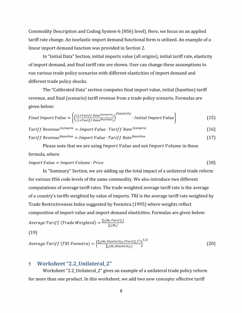
OR
Final Tariff Rate= �O if Column G=0 and Column H =1 Initial Tariff Rate if Column G=1Initial Tariff Rate if Column H=0
�
(26)
Please note that the formula for final imports value is now computed for bilateral
import values.
𝐹𝑖𝑛𝑎𝑙 𝐵𝑖𝑙𝑎𝑡𝑒𝑟𝑎𝑙 𝐼𝑚𝑝𝑜𝑟𝑡 𝑉𝑎𝑙𝑢𝑒 =
𝐼𝑛𝑖𝑡𝑖𝑎𝑙 𝐵𝑖𝑙𝑎𝑡𝑒𝑟𝑎𝑙 𝐼𝑚𝑝𝑜𝑟𝑡 𝑉𝑎𝑙𝑢𝑒 ∙ ��(1+𝑇𝑎𝑟𝑖𝑓𝑓 𝑅𝑎𝑡𝑒𝑆𝑐𝑒𝑛𝑎𝑟𝑖𝑜)∙(1+𝑉𝐴𝑇)�1+𝑇𝑎𝑟𝑖𝑓𝑓 𝑅𝑎𝑡𝑒𝐵𝑎𝑠𝑒𝑙𝑖𝑛𝑒�∙(1+𝑉𝐴𝑇)
�𝐸𝑙𝑎𝑠𝑡𝑖𝑐𝑖𝑡𝑦
� (27)
In Cell Range U1:X101, examples of how to compute total import value with a
trading partner for all products that are traded.
𝑀𝑖 = ∑ 𝑀𝑖𝑗
𝑗 (28)
where i denotes countries and j denotes products.
8 Worksheet “4.1_WTO_Unilateral” Worksheet “4.1_WTO_Unilateral” gives an example of a unilateral WTO trade reform
agreement for applied and bound tariff rates. In this example, one country conducts a trade
policy change. Here we focus on an applied tariff rate change. An isoelastic import demand
functional form is utilized. An example of a linear import demand function was provided in
Section 2.
While bilateral trade agreement involves two countries, a multilateral trade
agreement involves three or more countries who wish to regulate trade between the
nations without discrimination. Compared with bilateral trade agreements, multilateral
trade agreement can further reinforce and enhance the economic gains from international
trade.
WTO is the only international organization dealing with the global rules of trade
between nations. Its main function is to ensure that trade flows as smoothly, predictably
and freely as possible. The multilateral trading system is the WTO’s agreements, negotiated
and signed by a large majority of the world’s trading nations, and ratified in their
parliaments.
11

In “Initial Data” Section, initial imports value (all origins), initial tariff rate, 𝑉𝐴𝑇
(sales tax), bound rate, and elasticity of import demand. User can change these
assumptions to run various trade policy scenarios with different elasticities of import
demand and different trade policy shocks.
Final tariff rate depends on Swiss Formula (WTO 2012a) that uses a single
mathematical formula to produce:
1. a narrow range of final tariff rates from a wide set of initial tariffs
2. a maximum final rate, no matter how high the original tariff was.
A key feature is a number, which can be negotiated and plugged into the formula. It
is known as a “coefficient” (“A” in the formula below). This also determines the maximum
final tariff rate.
𝐹𝑖𝑛𝑎𝑙 𝑇𝑎𝑟𝑖𝑓𝑓 𝑅𝑎𝑡𝑒 = 𝑀𝑖𝑛 �𝐼𝑛𝑖𝑡𝑖𝑎𝑙 𝑇𝑎𝑟𝑖𝑓𝑓 𝑅𝑎𝑡𝑒, (𝐵𝑜𝑢𝑛𝑑 𝑅𝑎𝑡𝑒 ∙ 𝐴)(𝐵𝑜𝑢𝑛𝑑 𝑅𝑎𝑡𝑒 + 𝐴)� (29)
Please note that 𝐵𝑜𝑢𝑛𝑑 𝑅𝑎𝑡𝑒 is lowered in this example and the agreement affects
domestic prices and import volume only if the 𝐹𝑖𝑛𝑎𝑙 𝑇𝑎𝑟𝑖𝑓𝑓 𝑅𝑎𝑡𝑒 is lower than the
𝐼𝑛𝑖𝑡𝑖𝑎𝑙 𝑇𝑎𝑟𝑖𝑓𝑓 𝑅𝑎𝑡𝑒. 𝐵𝑜𝑢𝑛𝑑 𝑅𝑎𝑡𝑒 is the maximum rate of tariff allowed by WTO to any
member state for imports from another member state. In “Calibrated Data Section”, we
compute final imports value (all origins), initial tariff revenue, final tariff revenue, initial tax
revenue, and final tax revenue with formulas described above.
One important thing to note is that although the Swiss formula is used in this
example, there are other formulae that can be used to reduce and/or harmonize tariff rates.
These formulae can be part of the trade negotiations. Examples include proportional cuts in
tariffs, tiered formula in the WTO Harbinson proposal, among others. Jean, Laborde, Martin
(2005) provide a detailed discussion of various formulae that can be used in trade
negotiations as well as implications of using these different versions. Documentation of
TASTE (IFPRI 2012a) also gives an overview of different formulae to reduce tariffs in trade
negotiations.
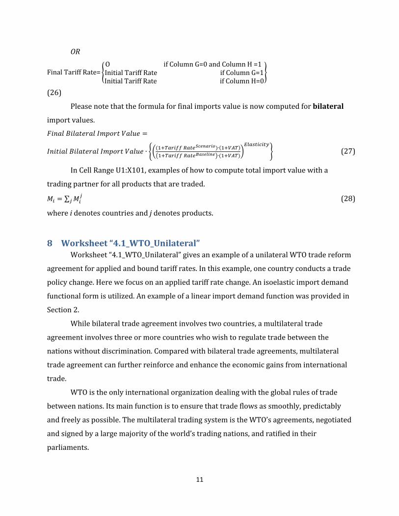
9 Worksheet “4.2_WTO_Bilateral” Worksheet “4.2_WTO_Bilateral” gives an example of a bilateral WTO trade reform
agreement for applied and bound tariff rates. In this worksheet, we have one country
12
trading with more than one partner for same products. Here we focus on an applied tariff
rate change. An isoelastic import demand functional form is utilized. An example of a linear
import demand function was provided in Section 2.
Again,
𝐹𝑖𝑛𝑎𝑙 𝑇𝑎𝑟𝑖𝑓𝑓 𝑅𝑎𝑡𝑒 = 𝑀𝑖𝑛 �𝐼𝑛𝑖𝑡𝑖𝑎𝑙 𝑇𝑎𝑟𝑖𝑓𝑓 𝑅𝑎𝑡𝑒, (𝐵𝑜𝑢𝑛𝑑 𝑅𝑎𝑡𝑒 ∙ 𝐴)(𝐵𝑜𝑢𝑛𝑑 𝑅𝑎𝑡𝑒 + 𝐴)� (30)
Please note that the value of Swiss coefficient is different in this worksheet. This
coefficient can be part of trade negotiations.
In “Calibrated Data Section”, we compute final imports (bilateral), initial tariff
revenue, final tariff revenue, initial tax revenue, and final tax revenue with formulas
described above.
10 Worksheet “4.3_WTO_MyExports” Worksheet “4.3_WTO_MyExports” shows the import demand of the partners of a
trading country. In this example, we are adding the concept of being a WTO member.
We introduce WTO members in Cell Range C13: C8146. A trade partner country is
member of the WTO if value is 1and not a member if value is 0. If a country is a WTO
member, it has a 𝐵𝑜𝑢𝑛𝑑 𝑅𝑎𝑡𝑒 that has been negotiated when becoming a member. If not a
member, 𝐵𝑜𝑢𝑛𝑑 𝑅𝑎𝑡𝑒 is given as 0. Exports of original country are given in Column D to the
trade partners in Column B.
Now 𝐹𝑖𝑛𝑎𝑙 𝑇𝑎𝑟𝑖𝑓𝑓 𝑅𝑎𝑡𝑒 not only depends on Swiss formula but also on trading
partner’s being a WTO member or not. In “Calibrated Data” section, we see below formula:
𝐹𝑖𝑛𝑎𝑙 𝑇𝑎𝑟𝑖𝑓𝑓 𝑅𝑎𝑡𝑒 = �𝐼𝑓 𝑊𝑇𝑂 𝑚𝑒𝑚𝑏𝑒𝑟 𝑀𝑖𝑛 �𝐼𝑛𝑖𝑡𝑖𝑎𝑙 𝑇𝑎𝑟𝑖𝑓𝑓 𝑅𝑎𝑡𝑒, (𝐵𝑜𝑢𝑛𝑑 𝑅𝑎𝑡𝑒∙𝐴)(𝐵𝑜𝑢𝑛𝑑 𝑅𝑎𝑡𝑒+𝐴)�
𝐼𝑓 𝑁𝑜𝑡 𝑊𝑇𝑂 𝑚𝑒𝑚𝑏𝑒𝑟 𝐼𝑛𝑖𝑡𝑖𝑎𝑙 𝑇𝑎𝑟𝑖𝑓𝑓 𝑅𝑎𝑡𝑒� (31)
𝐹𝑖𝑛𝑎𝑙 𝐸𝑥𝑝𝑜𝑟𝑡𝑠 = ��(1+𝑇𝑎𝑟𝑖𝑓𝑓 𝑅𝑎𝑡𝑒𝑆𝑐𝑒𝑛𝑎𝑟𝑖𝑜)�1+𝑇𝑎𝑟𝑖𝑓𝑓 𝑅𝑎𝑡𝑒𝐵𝑎𝑠𝑒𝑙𝑖𝑛𝑒�
�𝐸𝑙𝑎𝑠𝑡𝑖𝑐𝑖𝑡𝑦
∙ 𝐼𝑛𝑖𝑡𝑖𝑎𝑙 𝐸𝑥𝑝𝑜𝑟𝑡𝑠� (32)
In Cell Range N1:Q4, examples of how to compute total exports to a trading partner
for all products that are traded are shown.
𝑋𝑖 = ∑ 𝑋𝑖𝑗
𝑗 (33)
where i denotes countries and j denotes products.
13
In Cell Range S1:V4, examples of how to compute total exports of a product to all
trading partners are shown.
𝑋𝑗 = ∑ 𝑋𝑖𝑗
𝑖 (34)
where i denotes countries and j denotes products.
11 Data Sources Please note that the data and assumptions provided in this model can be changed or
enhanced by using other data sources. Below is a non-exhaustive list.
11.1 Trade and Tariff Data One of the data sources is the MAcMap-HS6 (IFPRI 2012b) that provides detailed
data on bound and applied tariff rates at HS6 level for the year 2004. It provides: (i) an
exhaustive coverage of preferential trade arrangements across the world; (ii) the
calculation of the ad valorem equivalent (AVE) for specific duties, acknowledging the
differentiated impact of such duties across exporters, depending on their export unit values;
(iii) the incorporation of tariff-rate quotas both through the AVE of the resulting protection
at the margin, and through the calculation of involved rents; (iv) an original aggregation
methodology, using a weighting scheme based on reference groups of countries, and
limiting the extent of the endogeneity bias inherent to the standard, import-weighted
average protection.
Another source is the TASTE program which has been designed to allow a large
number of users to analyze existing trade policies and perform tariff scenarios. It is based
on the MAcMap-HS6 database (version 2, base year 2004), and is designed to accompany
the version 7 GTAP database (IFPRI 2012a). It addresses several needs:
• Queries on the MAcMap-HS6 database and computation of aggregate tariffs (bound and
applied) at different sectoral and regional level (different aggregation methods
allowed);
• Simulations of tariff changes resulting from a trade policy scenario implemented at the
product (HS6) level. Outputs can be used in different models;
• Disaggregation tools for GTAP users in combination with the SPLITCOM software.
14

TASTE comes with a huge database of bilateral trade flows and of applied and
bound tariff rates distinguishing around 200 countries and 5000 HS6 goods.
World Integrated Trade Solution (WITS 2012) by World Bank is another important
tool. It is a software developed by the World Bank, in close collaboration and consultation
with various International Organizations including United Nations Conference on Trade
and Development (UNCTAD), International Trade Center (ITC), United Nations Statistical
Division (UNSD) and WTO. WITS gives you access to major international trade, tariffs and
non-tariff data compilations:
• The UN COMTRADE database maintained by the UNSD: Exports and imports by detailed
commodity and partner country
• The TRAINS maintained by the UNCTAD: Imports, Tariffs, Para-Tariffs & Non-Tariff
Measures at national tariff level
• The IDB and CTS databases maintained by the WTO: MFN Applied, Preferential & Bound
Tariffs at national tariff level
WTO website also provides international trade and market access data as well as
various publications (WTO 2012b). Domestic sources for countries include government
and ministerial websites, decrees, trade group publications among others.
11.2 Elasticities FAPRI elasticity data base (FAPRI 2012) provides demand and supply own price
elasticities. Some FAPRI publications that provide supply and demand elasticities are Yu et
al. (2011) and Fabiosa et al. (2010).
For import demand elasticities, please refer to Kee, Nicita and Olarreaga (2008)
which is published in World Bank (2012b). If users prefer to use alternative sources, they
should make sure that import demand elasticities have been estimated at free trade
international prices.
Trade and International Integration team of the World Bank Development Research
Group collects and disseminates data to support its own research activities and the global
trade policy agenda. Please refer to World Bank (2012c) for the various data sets to be
downloaded.
There will also be a future tariff data base provided through the AGRODEP website.
15

11.3 Effective tariff revenue Domestic Custom Authorities of countries would also publish tariff revenues that
are collected at different tariff line levels. A broad approximation can be computed at the
aggregated level using IMF figure on total custom duty collected and use the average rate
on all products.
16

12 Appendix I Figure 1 shows the supply, demand and imports of a net importing country. A
denotes Autarky equilibrium. In an open economy, country imports the good by paying the
world price plus the tariff rate. Consumer surplus is the sum of areas 1 and 2. Producer
surplus is area 3.
Figure 1: Consumer and producer surplus
17

13 Appendix II Figure 2 shows the effects of a change in import tariff rate on the supply, demand
and imports of a net importing country. A denotes Autarky equilibrium. Country imports
the good by paying the world price plus the 𝑡𝑎𝑟𝑖𝑓𝑓𝐵𝑎𝑠𝑒𝑙𝑖𝑛𝑒. After the tariff rate decline,
country pays the 𝑡𝑎𝑟𝑖𝑓𝑓𝑆𝑐𝑒𝑛𝑎𝑟𝑖𝑜. Initially the country produces 𝑆𝐵 and consumes 𝐷𝐵,
importing the difference (𝑀𝐵). After the decline in tariff rate to 𝑡𝑎𝑟𝑖𝑓𝑓𝑆𝑐𝑒𝑛𝑎𝑟𝑖𝑜 , country
imports more (𝑀𝑆) since domestic production declines to 𝑆𝑆 and domestic consumption
rises to 𝐷𝑆. Consumer surplus increases by the sum of areas 1, 2, 3, and 4. Area 3 also shows
the change in tariff revenue. Area 1 is the decline in producer surplus.
Figure 2: Effects of an import tariff
18
14 References Fabiosa, J. F., J. C. Beghin, F. Dong, A. Elobeid, S. Tokgoz, and T. Yu. 2010. “Land Allocation Effects of the Global Ethanol Surge: Predictions from the International FAPRI Model.”, Land Economics, Vol. 86 (4): 687-706. FAPRI. 2012. Food and Agricultural Policy Research Institute Elasticity Database. Available Online <http://www.fapri.iastate.edu/tools/elasticity.aspx> Feenstra, Robert C., 1995. "Estimating the effects of trade policy," Handbook of International Economics, Chapter 30 in: G. M. Grossman & K. Rogoff (ed.), IFPRI. 2012a. TASTE - Tariff Analytical and Simulation Tool for Economists. Available Online <http://www.ifpri.org/book-5080/ourwork/program/taste-tariff-analytical-and-simulation-tool-economists> IFPRI. 2012b. MacMapHS6 - Market Access Map at the HS6 level. Available Online <http://www.ifpri.org/book-5078/ourwork/program/macmap-hs6> Jean, S., D. Laborde, W. Martin, 2005. "Consequences of Alternative Formulas for Agricultural Tariff Cuts," Working Papers 2005-15, CEPII research center. Kee, H.L., A. Nicita and M. Olarreaga. 2008. “Import Demand Elasticities and Trade Distortions.” Review of Economics and Statistics, Vol. 90, No. 4: 666-682. WITS. 2012. World Integrated Trade Solution. Available Online <http://wits.worldbank.org/wits/> World Bank (2012a). Tariff Reform Impact Simulation Tool (TRIST). Available Online <http://web.worldbank.org/WBSITE/EXTERNAL/TOPICS/TRADE/0,,contentMDK:21537281~pagePK:210058~piPK:210062~theSitePK:239071,00.html> World Bank (2012b). Overall Trade Restrictiveness Indices and Import Demand Elasticities. Available Online <http://econ.worldbank.org/WBSITE/EXTERNAL/EXTDEC/EXTRESEARCH/0,,contentMDK:22574446~pagePK:64214825~piPK:64214943~theSitePK:469382,00.html> World Bank (2012c). Trade Policy Research. Available Online <http://econ.worldbank.org/programs/trade/tradepolicy> WTO (World Trade Organization). 2012a. “Agriculture Negotiations: Background Fact Sheet.” Available Online <http://www.wto.org/english/tratop_e/agric_e/agnegs_swissformula_e.htm#top>. WTO (World Trade Organization). 2012b. International trade and market access data. Available Online <http://www.wto.org/english/res_e/statis_e/statis_e.htm>
19

Yu, T., S. Tokgoz, E. Wailes, and E. Chavez. 2011. “A quantitative analysis of trade policy responses to higher world agricultural commodity prices.” Food Policy, Vol. 36: 545-561.
20