Estimating Impact in Partial vs. General Equilibrium:A Cautionary Tale from a Natural Experiment in Uganda∗

Jakob Svensson† David Yanagizawa-Drott‡

Preliminary.

August 2012

Abstract

This paper provides an example where sensible conclusions made in partial equilibrium are

offset by general equilibrium effects. We study the impact of an intervention that distributed

information on urban market prices of food crops through rural radio stations in Uganda. Using

a differences-in-differences approach and a partial equilibrium assumption of unaffected urban

market prices, the conclusion is the intervention lead to a substantial increase in average crop

revenue for farmers with access to the radio broadcasts, due to higher farm-gate prices and

a higher share of output sold to traders. This result is consistent with a simple model of the

agricultural market, where a small-scale policy intervention affects the willingness to sell by

reducing information frictions between farmers and rural-urban traders. However, as the radio

broadcasts were received by millions of farmers, the intervention had an aggregate effect on

urban market prices, thereby falsifying the partial equilibrium assumption and conclusion.

Instead, and consistent with the model when the policy intervention is large-scale, market

prices fell in response to the positive supply response by farmers with access to the broadcasts,

while crop revenues for farmers without access decreased as they responded to the lower price

level by decreasing market participation. When taking the general equilibrium effect on prices

and farmers without access to the broadcasts into account, the conclusion is the intervention

had no impact on average crop revenue, but large distributional consequences.

∗Acknowledgement: We thank Frances Nsonzi and the management team at Foodnet for their assistance. Weare grateful for comments and suggestions by Tessa Bold, Per Krusell, Daron Acemoglu, and seminar participants atHarvard Kennedy School, IIES, University of Frankfurt, and Centre d’Economie de la Sorbonne. Financial supportfrom the Swedish International Development Agency, Department for Research Cooperation and Handelsbanken’sResearch Foundations is gratefully acknowledged.

†IIES, Stockholm University‡Harvard University

1

1 Introduction

The bulk of empirical work using microdata, particularly in development economics, engages in

partial equilibrium comparisons (Acemoglu, 2010). Although general equilibrium interactions

can offset or even reverse sensible partial equilibrium conclusions (Heckman, Lochner, and Taber

1998), it also requires variation in exposure at the level of the economy; i.e. requires that the gen-

eral equilibrium effects take place at the local level, to be credibly estimated using micro econo-

metric approaches (Duflo, 2004). Thus most policy evaluation studies focus on impact in partial

equilibrium.

In this paper, we assess the impact of providing price information in agricultural markets. This

is an important question, as farmers’ lack of access to updated market prices, and the frictions that

may entail, is a common explanation put forward to explain the low levels of market exchange in

Sub-Saharan Africa (World Bank, 2007).1 As 75 percent of the world’s poor live in rural areas

and make their livelihood mainly from farming crops, efforts to increase farmers’ willingness and

return from engaging in market exchange is high on the policy agenda and ICT (Information and

Communications Technologies) based interventions, where market prices are disseminated through

radio, mobile, or internet, are now common in many parts of the developing world.

In this paper we use data from a policy experiment in Uganda aimed at increasing small-scale

farmers willingness and return from engaging in market exchange by providing information on ur-

ban crop market prices. The Market Information Service (MIS) in Uganda, collected weekly data

on market prices for a set of agricultural commodities in a subset of Uganda’s districts and dissemi-

nated the information to farmers through local FM radio stations. We contrast the estimated impact

of the intervention under a partial equilibrium assumption and a general equilibrium assumption,

which lead to very different conclusions. Under the assuming that the intervention was done on a

small-scale and partial equilibrium analysis is suitable, the intervention had large and positive ef-

fects on farmers crop revenues. However, millions of farmers had access to the intervention, which

led to general equilibrium effects on the price. When relaxing the assumption of fixed market price

and allowing for behavioral responses among farmer without direct access to the intervention, the

estimates imply negligible aggregate effects on crop revenue but large distributional consequences.

We thus provide an example where sensible conclusions made in partial equilibrium are offset by

general equilibrium effects.

To this end, we first present a simple general equilibrium model of the agricultural economy. In

the model, asymmetric information gives rise to contracting frictions between farmers and traders,

as rent-seeking traders operating in rural areas with low availability of updated price information

1In Uganda, for example, only around 25 percent of output produced by small-scale farmer is sold and less than

one-third (and for some crops as few as one-tenth) of the farmers participate actively in market exchange (as sellers),

although sales of crops is the main (sole) source of cash income for many farmers.

2

have incentives to claim that prices in urban markets are lower than what they actually are. To

reduce these incentives, farmers cut down the amount they sell unless the trader reports a high

price. As a result, market exchange will be sub-optimally low. Providing farmers with access

to price information reduces these frictions, resulting in both increased market participation and

higher farm gate prices. In partial equilibrium, farmers that receive access to up-to-date market

price information ("informed farmers") are better off, while uninformed farmers are unaffected.

Allowing urban market prices to respond to the increased supply by informed farmers, however,

change the equilibrium outcomes. Uninformed farmers then faces lower market prices and respond

by reducing their market participation.

To assess the predictions of the model, we use variation in access to market price information

over time, across space, and between crops, and exploit the fact that market prices are set on local

(district) markets that are not (fully) integrated. We first show that market prices responded to the

MIS intervention, and the more so the higher the share of informed farmers. Specifically, a one

percent increase in number of informed farmers resulted in a 0.36 percent fall in district market

prices. We then exploit the household survey data to investigate the effects on individual level.

Under fairly weak identifying assumptions, we can estimate the difference in mean outcomes (in

general equilibrium) between informed and uninformed farmers. We find that access to market

information increased the likelihood of selling the crop by about 3 percentage points, or 13 %, in

the informed group, while market participation among uninformed farmers fell by 6 percentage

points; that is a 9 percentage point difference in market participation between informed and un-

informed farmers as a result of the intervention. We find a similar effect for the total margin; i.e.

share sold, with informed farmers selling more (a 14% increase) and uninformed farmers selling

less (24% reduction). Informed farmers also benefitted from higher farm-gate prices. Ignoring the

general equilibrium effects, our result would suggest a large, positive, effect from the MIS inter-

vention, with crop revenue of informed farmers increasing by 75%, albeit starting from a low level.

However, in general equilibrium, we estimate a much more modest increase in crop revenue for

the informed farmers (13% increase), while uninformed farmers saw their crop income drop by an

estimated 35 %. The aggregate impact of the intervention on average crop revenue was negligible,

but it had large distributional consequences: Consumers benefited from lower prices; informed

farmers benefited from higher farm revenues, while crop income fell for uninformed farmers.

The paper relates to a small and recent literature on the effects of improved access to market

information in the agricultural sector.2 Our work differs in important ways. First, the paper high-

2Focusing on the ability to exploit arbitrage opportunities, Jensen (2007) evaluates the effects of the introduction

of mobile phones on market outcomes in the fishing industry in Kerala, India. He finds that by improving fishermen’s

and traders’ ability to communicate over large distances, the introduction of mobile phones improved arbitrage oppor-

tunities and resulted in reduced waste and decreased price dispersion across geographic markets. Studying traders’

search behavior in Niger, Aker (2008) finds similar effects on price dispersions across grain markets when mobile

3

lights the importance of assessing general equilibrium effects when analyzing policy interventions

based on microdata, as stressed by Heckman, Lochner, and Taber (1998) and Acemoglu (2010).

Second, as in Goyal (2010) we study the impact of increasing farmer access to price information,

rather than traders access to information.3 Third, since farmers in Uganda almost exclusively sell

their crops to traders at the farm-gate, we do not study the decision on where or to whom to sell the

output. Instead, we investigate the impact on the economic exchange at the farm-gate conditional

on the farmers’ access to information about the prevailing market price.

The remainder of this paper proceeds as follows: Section 2 discusses the institutional setup,

including the Market Information Service project. The model is presented in section 3. Sections 4

and 5 discuss the data and the empirical strategy. The results are presented in section 5. Section 6

conducts robustness checks and Section 7 concludes.

2 Uganda’s Agricultural Sector

Uganda’s economy is predominantly agrarian. The agricultural sector employs roughly 80% of the

labor force and is the main source of livelihood for more than 85% of the population.4 Almost

94% of the agricultural production take place on smallholder plots, including virtually all food

production (Ministry of Finance, 2008). Detailed aggregate data for all crops is not available, but

for maize, for example, it is estimated that 95% of the households engaged in maize production are

small-scale farmers (with land holdings of 0.2-0.5ha), contributing over 75% of the marketable sur-

plus of maize. Medium scale commercial farmers with 0.8-2.0ha of land under maize production

contribute the remaining 25% (RATES Center, 2003).

Due to poor transportation infrastructure and lack of storage facilities, small-scale subsistence

farmers sell off most of their surplus produce to rural traders immediately after harvest. For maize,

rural traders, who operate in villages, constitute over 90% of the total number of maize traders and

handle two-thirds of all traded maize. Typically, traders traverse villages on bicycles and pick-ups

phones were introduced. Both these studies focus on technology improvements that lower search costs in the decision

on where to sell the output. Goyal (2010) exploits variation induced by the entry of a large private soybeans buyer

(ITC) in Madhya Pradesh, India. She finds that providing farmers with information about wholesale prices of soybean

in local markets and an outside option to sell directly at known prices to ITC, resulted in an increase in the average

price of soybean in the local market. The finding is consistent with a model where information about current market

prices and/or the introduction of a new outside option increased competition between the local traders.3This is not to say that the information disseminated through radio did not contain any new information to traders.

However, given that traders travels back and forth to the market places on a daily basis while farmers do not, it is

clear that the relative information supplied to farmers was much larger. We also find no evidence of decreased price

dispersion across districts after the radio disseminations started transmissions. Even if traders were benefitting, the

empirical strategy identifies the farmer’s access to price information.4The main crops include both cash crops, such as coffee, tea, cotton, tobacco, and cocoa, and food crops,including

plantains, maize, cassava, maize, beans, millet and sweet potatoes, and recently a smaller set of horticultural produce.

4

procuring produce at farm-gate prices on a cash basis. Moreover, almost no farmers engage in

long-term contractual arrangements with a trader.5 Instead, most farmers engage with the market

through traders on an informal manner, resulting in spot contracts between farmers and traders.

Traders either work independently or as agents of larger urban traders. Since they travel back-

and-forth to the market, they are often well-informed, at least about the price in the district market

where they are active (RATES Center, 2003).

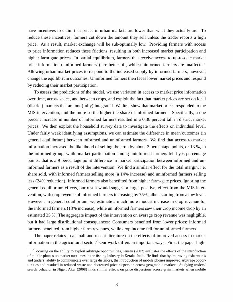
Prices on most cash- and food crops vary greatly in district markets in Uganda over time. As

an illustration, figure 1 depicts the weekly market price for cassava in the Kasese district market

center (the coefficient of variation over time is 0.28, close to the mean of 0.24). Given these price

variations, it is not surprising that farmers in Uganda view getting market information as one of

their highest priorities (Ferris, 2004).

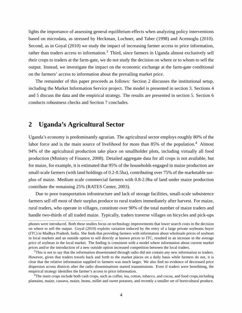
Prices also vary greatly across locations. Figure 2 plots the market price of beans during week

20 in 2001 across the participating MIS-districts. The variation in prices across districts at a given

point in time suggests that to the extent that farmers sell their output to traders located in their

own district, the market price in that district, rather than the average price in the country, is the

key statistic. Figure 2 also suggests that the lack of adequate transportation infrastructure makes

it difficult to exploit arbitrage across markets, thus implying that prices can be systematically

different across space at a given point in time.

2.1 The Market Information Service

In 2000, the Market Information Service project was initiated by two agricultural research orga-

nizations (IITA and ASARECA) in association with the Ministry of Trade, Tourism and Industry

in Uganda. The starting point of the project was survey data indicating that most farmers had

limited knowledge of the current market prices in the main district market centers, and scarce in-

formation on price movements and market trends. By providing accurate, timely and appropriate

information, the assumption was that small-scale farmers would be able to make better decisions

about what to produce and where to sell their output. Timely and accurate information would also

improve farmers’ bargaining position vis-à-vis local and regional traders.

In 2004, the Market Information Service was operating in 21 districts in Uganda.6 Figure 1

shows a map of participating districts. The project collected data, on a weekly basis, on market

prices for 19 agricultural commodities. In practice, however, the MIS regularly reported prices

5In a survey on ten districts, Ferris et al. (2006) report that only 3% of the farmers were trading on the basis of

long-term contractual arrangements.6The total number of districts in 2004 was 56. Not all districts could be included in the MIS project because for

budget and administrative reasons.

5

primarily on seven main food crops in Uganda (see details below): Beans, Cassava, Groundnuts,

Maize, Millet and Sweet potatoes.

In each MIS district, price information was processed and disseminated through various radio

stations. Price information was broadcast both weekly (a 15-minute radio program) and daily (a

2-4 minute news bulletin) in altogether eight local languages. The MIS targeted the most popular

radio stations and in 2004, the MIS was estimated to reach seven of Uganda’s twenty-four million

people each week (Ferris, 2004).7 The intervention, therefore, was on a large-scale.

3 A simple model of price information and agricultural market

exchange

We model an economy consisting of a continuum of atomistic small-scale rural farmers, rural-

urban traders, and consumers in an urban center. There is one good (crop) which is produced by

the farmers, bought by traders at farmers’ farm-gates, and resold to consumers in the urban market

center. The model consists of two parts. In the first part, we model how farm-gate prices and

quantity are set, conditional on farmers’ access to information, and taking (urban) market prices

as given. In the second part, we endogenize the market prices in the urban market center traders

sell the crops bought from farmers. This then pins down the equilibrium quantities and prices both

in the urban market center and at the farm-gates. The model will have two key features reflecting

the conditions in many low-income countries, including Uganda as described above. First, since

traders constantly travel back and forth between the urban market and the rural areas, the market

price (and the demand shock) will be observable to traders. Rural farmers do not observe the

market price, however. Second, competition between traders at the farm-gate is imperfect. This

will then give rise to inefficiencies due to asymmetric information between traders and farmers.

3.1 The Farm-Gate Equilibrium

Let each farmer produce one crop of quantity Q, of which he can sell q ≤ Q to a trader and

consume the rest, c = Q− q. We are interested in how much a farmer sells of what he produces and

the prices he receives for his crops (henceforth "farm-gate price"), conditional on what information

he has of the current retail market price (henceforth "market price"). The farmer’s payoff function

7The MIS project initially bought air-time from the radio stations for the radio program. Interestingly, because

of the popularity of the program among farmers, several commercial radio stations started to transmit the programs

without public funds.

6

is

(1) U = R+ u(Q− q) ,

where R is the total amount paid to the farmer (for q) and u(0) = 0, u′(c) > 0, u′′(c) < 0,

u′′′(c) > 0.

Competition between traders at each farm-gate is imperfect.8 For simplicity, we assume that

there is one trader at the farm-gate to whom the farmer can sell. The trader’s profit is

(2) Π = mq− R ,

where m is the current market price in the urban retail market.9 We assume there are three possible

market prices m1 < m2 < m3, that are realized with probability π1, π2, π3, respectively (and

summing up to one).10

The economy consists of a continuum of atomistic farmers, with measure one. The are two

types of farmers: a share r informed (knows the realized retail market price) farmers and a share

(1− r) uninformed (cannot observe the realized retail market price) farmers, with r ∈ [0, 1].In this set-up, the farmer is the principal that offers a take-it-or-leave contract to the trader on

quantity q(m) and per-unit price p(m), or, analogously, revenue R(m) = p(m)q(m).11

3.1.1 The uninformed farmer

The uninformed farmer cannot observe the market price but knows the distribution. This is essen-

tially a standard bilateral contracting model, or monopolistic screening, under hidden information.

The farmer suggests a contract conditional on the market price that the trader reports. The unin-

formed farmer’s problem is that the trader, who knows the market price, has incentives to claim

that the market price is lower than it actually is. However, since the trader is more eager to buy

when the market price is high, the farmer can possibly reduce the trader’s incentives to report a low

market price by cutting down the amount he sells when the trader reports a low market price. By re-

ducing the trader’s incentives to report a low market price, the farmer can reduce the informational

8Reasons for this could be high fixed costs (buying a truck) for becoming a trader, or collusion between traders.

Fafchamps and Minten (2001) and Ferris (2004) provide evidence in favor of the assumption.9Transport costs t could easily be added, for example the linear cost tq, for the trader without changing the main

results.10Solving the farm-gate equilibrium with continuous prices does not change the main results. We choose discrete

prices because it is more tractable.11An alternative set-up is to assume that the buyer (trader) offers the seller (farmer) a take-it-or-leave-it contract.

7

rent of the trader.

We are interested in the menu of contracts{(qU

j , mj; j = 1, 2, 3}

where superscript U denotes

equilibrium outcomes when the farmers is uninformed. The optimal contract is defined by the

following maximization program

(3) max{(qj,Rj)}

3

∑j=1

π j[Rj + u(Q− qj)

]subject to

(4) mjqj − Rj ≥ 0 for all j

(5) mjqj − Rj ≥ mjqk − Rk for all j,k

where (4) are the IR-constraints and (5) the incentive-compatability (IC) constraints. Note that

only one of the IR constraints binds since

(6) m3q3 − R3 ≥ m3q2 − R2 ≥ m2q2 − R2 ≥ m2q1 − R1 ≥ m1q1 − R1 ≥ 0

Note further that the Spence-Mirrless single-crossing condition holds, implying that the number of

incentive constraints can be reduced to a smaller set of local downward incentive constraints and a

monotonicity condition. The farmer’s problem can thus be stated as,12

(7) max{(qj,Rj)}

3

∑j=1

π j[Rj + u(Q− qj)

]subject to

(8) m1q1 − R1 = 0

12The Spence-Mirrless single-crossing condition is

∂

∂m

[− ∂U/∂q

∂U/∂R

]=

∂

∂m

[− m−1

]> 0

For details how to solve contract problems of this form see Bolton and Dewatripont (2005).

8

(9) mjqj − Rj = mjqj−1 − Rj−1 for all j > 1

(10) qj ≥ qk if mj ≥ mk

To solve the constrained problem we set up the Lagrangian, assuming the monotonicity condi-

tion (10) holds. That is

L = max3

∑j=1

{π j[Rj + u(Q− qj)

]+ λj

[mjqj −mjqj−1 − Rj + Rj−1

]}+µ [m1q1 − R1](11)

where λi is the Lagrange multiplier associated with the IC-constraint at price mi, and µ is the

multiplier associated with the IR-constraint (8). Rewriting the first-order conditions yields the

following conditions for qj,

(12) −u′(Q− qU3 ) +m3 = 0

(13) −u′(Q− qU2 ) +m2 −

π3

π2(m3 −m2) ≤ 0

(14) −u′(Q− qU1 ) +m1 −

(π2 + π3)

π1(m2 −m1) ≤ 0 .

The monotonicity condition (10) holds if assumption 1 holds, which we assume is the case.

(15) Assumption 1:1

π1(m2 −m1) ≥

π3

π2(m3 −m2)

Three results are immediately apperent from (12)-(14). First, qU3 = Q− u−1

c (m3); i.e., the first-

best quantity. This is the well-known "efficiency at the top" result. Second, qU1 and qU

2 are lower

than the first-best quantities where the size of the distortion, qFBj − qU

j , is increasing in the potential

size of the informational rent (mj+1 −mj) for j = 1, 2. Third, the optimal solution might involve

9

no market exchange; i.e. qUj = 0. Specifically, given that assumption 2 holds, uninformed farmers

do not sell at the lowest market price.

(16) Assumption 2: u′(Q) >1

π1m1 −

1− π1

π1m2

From the IR-constraints we can also determine the farm-gate prices, given by

pU1 = {no exchange}(17)

pU2 = m2(18)

pU3 = m3 −

qU2

qU3(m3 −m2)(19)

3.1.2 The informed farmer

Now instead assume that the farmer knows the current market price. The constrained maximization

problem is then

(20) max{(qj,Rj)}

3

∑j=1

π j[Rj + u(Q− qj)

]subject to

(21) mjqj − Rj ≥ 0 for all j,

where (21) is the trader’s individual rationality constraints (IR).

Since the farmer has no incentives to relax the IR-constraints, we can solve for Rj from (21)

and substitute into the maximimand (20). This yields an identical problem as that in the first-best.

Thus, quantity sold under full information, qIj , is equal to the first-best quantities

(22) qjj = Q− u−1

c (mj), j = 1, 2, 3

From the IR-constraint we can solve for the farmer’s revenue, Ri, and the unit price

(23) pjj ≡

Rj

qj= mj.

10

3.2 The Urban Market Price

So far we have taken prices as given. In this section, we endogenize the market prices. Assume

each trader sells all the crops that he has purchased from the farmers in an urban market center.

Let the set of traders be large such that each trader is a price taker in the retail market at the urban

center. Assume further that farmers vary in the minimum amount they are willing to buy from an

individual farmer, such that a trade takes place provided that qkj ≥ η, where η is drawn from the

uniform distribution U[0, 1]. As our focus is on the difference between informed and uninformed

farmers, we assume qI2 > 1 > qU

2 , implying that the minimum amount to buy constraint only binds

for (some) uninformed farmers at the market price m2.

The supply is then a function of the market price and the fraction of informed farmers,

(24) S(mj, r) = rρIj q

Ij + (1− r)ρU

j qUj , j = 1, 2, 3

where ρkj is the probability that a farmer of type k = {I, U} sells at price mj. Note that ρU

1 = 0 ,

ρU2 = qU

2 (m∗2 , m∗3), and ρI

1 = qI1(m

∗1).

We can consider the demand coming from consumers consisting of urban non-agricultural

households. For simplicity, we assume a linear demand function

(25) D(mj, εj) = d− δmj + εj, j = 1, 2, 3

where εj is an aggregate demand shock. We assume there are three possible demand shocks ε1 <

ε2 < ε3, that are realized with probability π1, π2, π3, respectively (and summing up to one). We

can think of the demand shock emanating from shocks in urban wages due to import or export

price shocks for non-agricultural commodities. Key is that the demand shocks give rise to market

price shocks that are unobservable to uninformed farmers but observable to traders and informed

farmers.

The general equilibrium (the retail market equilibrium and the farm-gate equilibrium) is pinned

by three market clearing conditions

(26) d− δm∗1 + ε1 = rρI3qI

1(m∗1)

11

(27) d− δm∗2 + ε2 = rqI2(m

∗2) + (1− r)ρU

2 qU2 (m

∗2 , m∗3)

(28) d− δm∗3 + ε3 = qI3(m

∗3)

together with the farm gate equilibrium quantities implicitly defined by (12)-(13), and (22).

3.3 Predictions and intuitions

The model provides a set of testable predictions. We summarize the main ones below. Our focus

is to estimate the effects of disseminating crop market prices, through the Market Information

Services (MIS), on prices and market participation of small-scale farmers in partial and general

equilibrium. The model highlights two mechanisms. First, the dissemination of information should

reduce distortions and shift surplus from the buyer to the farmer and thereby increase market

participation by farmers that can access the MIS. This is the main effect in partial equilibrium.

Second, through the change in supply, dissemination of information will change both the mean

and distribution of market prices. This is the general equilibrium effect.

Let x(m) be some outcome of interest (share sold for example) as a function of the vector of

prices m = {m1, m2, m3}. Then the partial equilibrium average treatment estimate of the Market

Information System is

(29) MISPE [x(m)] = E[

xI(m)]− E

[xU(m)

]where xI(m) [xU(m)] represents the outcome for farmers that do [not] access the MIS, and PEdenotes that the market price distribution (m) is assumed to be fixed. MISPE would be the relevant

measure to use if the intervention was done on a small scale; i.e. when it is reasonable to assume

that aggregate prices do not repond to the intervention. For a large scale policy experiment (like

the Market Information Services), however, or when scaling up a pilot project, prices are likely

to change. Thus, xU(m) cannot be used as a counterfactual outcome. There are therefore two

treatment effects, MISIGE[xI(m(r))

]and MISU

GE[xU(m(r))

], for informed and uninformed

farmers, respectively, where

(30) MISIGE

[xI(m)

]= E

[xI(m(r))

]− E

[xU(m(0))

]

12

and

(31) MISUGE

[xU(m)

]= E

[xU(m(r))

]− E

[xU(m(0))

]and where the subscripts GE denotes that market prices are endogenously determined; i.e., these

are the treatment effects in general equilibrium. In (30)-(31), E[xk(m(r))

]is the mean outcome

for a farmer of type k = {I, U} when a share r of farmers in the market accesses the MIS.

We are also interested in the average difference, denoted ∆MISGE [x(m)], in outcomes be-

tween informed and uninformed farmers when a share r of the farmers access the MIS; i.e.

(32) ∆MISGE [x(m)] = E[

xI(m(r))− xU(m(r))]

where ∆MISGE = MISIGE −MISU

GE.

We focus on five outcome variables: (i) The probability that the farmer engages in mar-

ket exchange (i.e., the extensive margin), ρU(m(r)) = 1 − π1 + π2qU2 (m(r)); (ii) The mean

share sold, E [s(m(r))] = E [q(m(r))/Q]; (iii) Farm-gate prices, p(m(r)); (iv) Crop revenues

R(m(r)) = p(m(r))q(m(r)); and (v) Market prices, m(r) = ∑ π jmj(r). We summarize the

predictions for the main outcome variables below.

Prediction 1. Dissemination of information on market prices on a large scale results in a lower av-

erage market price and the more so the higher is the share of informed farmers; i.e. ∂E [m(r)]/∂r <0.

Prediction 2. Disseminating information on market prices results in increased market partic-

ipation by those that can access information (informed farmers) and reduce market participa-

tion by those that cannot access information (uninformed farmers): i.e. MISIGE [s(m)] > 0,

MISIGE [ρ(m)] > 0, MISU

GE [s(m)] < 0 and MISUGE [ρ(m)] < 0. The effect on the average

farm-gate price E [p(m)] is indeterminate, while crop revenues for informed farmers increase and

crop revenues for uninformed farmer fall; i.e., MISIGE [π(m)] > 0 and MISU

GE [π(m)] < 0.

The intuition behind these results are straightforward. By disseminating information on market

prices, a share r of farmers become informed. Informed farmers do not have to sacrifice allocative

efficiency, or give up informational rents, to incentivize traders and therefore sell a larger share

of their output. As a consequence, the aggregate supply curve shifts outward and the more so the

higher is r. This shift in supply shifts the market price distribution and leads to a lower average

market price. As a result, uninformed farmers face on average lower farm-gate prices and therefore

reduce the amount they sell. Moreover, as prices fall, a higher share of uninformed farmers will

13

hit the minimum amount to sell constraint, thus also having an impact on the extensive margin.

MISIGE [p(m)] and MISU

GE [p(m)] are indeterminate. This is driven by the fact that becoming

informed has two effects on the farm-gate price: a direct incentive effect (positive) and an indirect

selection effect (negative). The incentive effect is positive since, conditional on a market price,

the informed farmer does not to give up informational rents to incentivize the trader. The selec-

tion effect, however, is negative since the informed farmer is willing to sell at (low) prices where

uninformed farmers are not, leading to a lower average farm-gate price.

4 Data

To test the predictions of the model, we want to measure whether a farmer is informed about the

market price, whether he engages in market exchange (ρi), the share of output sold (si), the farm-

gate price per unit sold (pi), crop revenues (πi), and market prices (mi). We are interested in

whether the Uganda Market Information Service that informed farmers about prevailing market

prices through local radio stations affected the outcome variables as predicted by the model.

We use three data sets: The Uganda National Household Survey 1999/2000 and 2004/2005

(hereafter UNHS 1999 and UNHS 2005) and data from the Market Information Service, provided

by Foodnet. The two household surveys include a full crop module, enabling us to calculate

farm-gate prices for crops sold, pi in the model, as well as measures of market participation on

both the extensive (ρ) and intensive (s) margins. The farmer data is measured at the plot level.

Summary statistics of the UNHS 1999 and 2005 are reported in table 1. The data from the Market

Information Service contains weekly data on collected urban market prices (from 2000 to 2005,

with some missing data). There is one urban market per district. The broadcasts were phased in,

starting in 2000 for the earliest district (Kampala) and completed by 2004.13 Using the UNHS

1999 dataset, we are able to use data from before the broadcast started. By using the UNHS 2005

dataset, we can use data for when the MIS was fully operational. In addition, for a subset of eight

districts, we have been able to collect information on the exact month in which broadcasts started.

4.1 Outcomes (ρ, s, p, m)

In our sample of the UNHS 1999 and 2005 datasets, there are 7960 and 5733 farmers, respectively.

Each farmer in the dataset produces one crop or more. We use crop level data which contains

information on what type of crop that is produced, the quantity produced, the quantity sold, and

13We drop the capital Kampala from our sample since there are no rural farmers in Kampala.

14

the price for the quantity sold. We also have access to a subset of the MIS radio scripts that were

used for the broadcasts. They show that there were some minor crops for which price information

was collected but very seldom broadcast. We use the main MIS crops, defined as those that were

reported in radio scripts on average at least once per month in 2004 and for which we have at least

1,000 data points (farmer plots) in the 2005 UNHS survey.14 The main MIS crops constitue 76%

of the reported MIS crop observations in the crop surveys.

We take a conservative approach with respect to outliers, all of which clearly seem to be a

result of misreporting. Thus, we drop all price observations with a reported unit price (the survey

contains information on the quantity produced of each crop, the quantity sold, and the total value of

the sale) higher than the highest reported weekly market price across all MIS district market centers

and we drop all price observations with a unit price below roughly 0.01US$ (which corresponds to

dropping all observations below the 1th percentile of the distribution for each crop). We also drop

observations with a higher quantity sold than harvested.

We use a similar rule to define control crops (non-MIS crops). Specifically the control crops

are those crops for which the MIS did not collect data for and that constitute at least one percent

of the reported non-MIS crops in the 2005 UNHS survey. We drop coffee since the Uganda Cof-

fee Development Authority (UCDA) runs a similar radio program for coffee in the main coffee

producing areas of Uganda.

For each crop, we construct an indicator variable equal to one if any of the output was sold, and

zero otherwise, as well as the share of the output that was sold.15 For farm-gate prices, we then

calculate the per kilogram price by dividing the total price by the quantity sold (in kilograms).16

We can then calculate the standardized farm-gate price.17

The UNHS 1999 and 2005 datasets also have information on whether the farmer owns a radio,

whether the farmer sold directly to the district market center and a quiz testing the farmer’s knowl-

edge of agricultural technology. The latter variable consists of seven multiple answer questions.18

We construct a variable measuring the fraction of correct answers by the farmer.

141,000 plots correspond to roughly 1% of the reported MIS crops. We also exclude Bananas/Matooke since the

MIS only reported one type of Banana/Matooke price while the crop modules list three types of plantain banana crops

(Matooke) and we were unable to separate for which one there were broadcasts.15In Uganda, there are two growing seasons per year. For each UNHS dataset, the crop data contains information

for each season.16The datasets also contain information on type of buyer. In 2005, 70% of the output were sold to a private trader in

the household’s village, 16% directly to another consumer or neighbor/relative, 9% at the district’s market center, and

5% to "other type of buyers". For simplicity, although the output is not always literally sold to a private trader at the

farm-gate, we label the price of all transaction types as the "farm-gate price".17That is, pij = ( p̃ij − p̄j)/σj, where p̃ij is the farm-gate price/kilogram in Uganda Shillings received for the sold

quantity of crop j by household i; p̄j is the mean farm-gate price in the sample, and σj is the corresponding standard

deviation.18Such as: Which of the following cassava planting methods provides better yields? 1. Vertically planted sticks; 2.

Horizontally planted sticks; 3. Both; 4. Don’t know.

15

For urban market prices, we use the MIS data provided by Foodnet. By exploiting the data

for the subset of eight districts where we know the month in which the broadcasts started, we can

divide the ten districts into early and late MIS districts. The early districts received broadcasts

starting in February 2001 and the late districts received broadcasts starting in September 2002.19

5 Empirical Strategy

This section outlines how we estimate the predictions of the model. We first present the coefficient

of interest and the empirical challenges of estimating it. We then present our empirical strategy

and specifications for how we estimate the effects.

5.1 Prediction 1: Market Price

Prediction 1 implies that when the share of informed farmers increases, the prices in the urban

retail market should decrease due to increased supply. To test this prediction, we use the market

price data from the urban markets and estimate the following main specification20

(33) log(m)cdt = β1(idistd × post)dt + γt + µcd + εcdt ,

where mcdt is the price of crop t in the main urban market of district d, in week t. The variable

idistd is a dummy variable indicating if the district received broadcasts starting in February 2002,

and zero if the district did not receive broadcasts until after the sample period. postdt is a dummy

variable indicating post-February 2002, and zero if it is pre-February 2002. Since the broadcasts

increased the number of informed farmers, by prediction 1 we expect β < 0.

(34)

log(m)cdt = β1(idist× post)cdt + β2(post× r̄)cdt + β3(idist× post× r̄)cdt + ηt + µcd + εcdt

where r̄ is the percentage of farmers in the district. with radio.

19The early districts are Jinja, Kabale, Masindi, Mbarara, and Soroti. The late districts are Gulu, Mbale, and Tororo.20The urban market price data contains data both on off-lorry prices and retail prices. We use the off-lorry prices as

these are what is paid to the traders. The two prices are naturally very similar: the correlation is 0.96.

16

Identifying assumptions : In equation (33), the diff-in-diff assumption is that in the absence

of price information broadcasts, early and late MIS districts would have parallel trends in mar-

ket prices. Similarly, in equation (34), we assume that radio farmers listen to the radio and are

informed, while farmers without radio are uninformed. Most importantly, we assume that in the

absence of broadcasts, the market price in districts with larger fraction of farmers with radio would

have parallel trends with districts with a smaller fraction of farmers with radio.

Under these assumptions, by prediction 1 we expect β3 = βm < 0.21 It is worth noting that if

some farmers with radio are uninformed (e.g. because they do not listen to the radio), or if farmers

without radio are informed anyways (e.g. by talking to informed farmers with radio), then we will

underestimate the true effects. In this case, the estimated β4 and β5 can be interpreted as lower

bounds of β3 < βm.To assess this assumption, we run a set of placebo regressions using samples

5.2 Prediction 2: Farm-Gate Outcomes

To test prediction 2, we exploit variation across time (before and after broadcasts begin), radio

ownership (of the farmer), crops (i.e. included or not included in the broadcasts), and districts

(participating in the MIS program). By exploiting variation across crops we are able to use farmer

fixed effects, which will be our most restrictive specification. We estimate two triple differences

(DDD) specifications.

5.2.1 DDD over time

The first DDD specfication is:

(35)

yicdt = β1ricdt+ β2(r× post)icdt+ β3(r× ic)icdt+ β4(ic× post)icdt+ β5(ic× post× r)icdt+ ηt+µcd+ εicdt.

where yicdt is the outcome of farmer i in district d producing crop c at time t. The variable ricdt

is a dummy variable equal to one if the farmer owns a radio, post is a dummy variable equal to

one if the observation is after the broadcasts started (i.e. the 2005 UNHS survey), and zero if it

is from before (UNHS 1999). icd is a dummy equal to one if the farmer’s crop is included in the

set of broadcasted crops. We use year fixed effects and district-by-crop fixed effects µdc. Our key

outcome variables are: ln(sicdt), the log of the share of output sold (i.e. the total margin)22; ρicdt,

21Notice the slight abuse of the notation, since we are using logged outcome variables for the total margin and

revenue in the regression, while in the model they are in levels.22To deal with undefined log function at zero, we add 1 kilogram to the true amount sold.

17

an indicator variable equal to one if the farmer sold any of his crop c output (i.e. the extensive

margin); picdt, the standardized farm-gate price per kilogram received for crop c by farmer i, and;

Ricdt, is the crop c revenue of farmer i. The main regressions use data from MIS districts only. We

cluster the standard errors at the district-crop level.

Identifying assumption in equation (35): Farmers with radio are informed and farmers without

radio are uninformed. Farmer selection into radio ownership may be different depending on the

crop grown, but this selection is constant over time.

Under these assumptions, by predictions 2 we will use OLS to consistently estimate:

• Extensive Margin: β5 = βρ > 0 and β4ρ = γρ < 0.

• Total Margin: β5 = βs > 0 and β4ρ = γs < 0.

• Farm-Gate Price: β5 = βp ≶ 0 and β4 = γp ≶ 0.

• Revenue: β5 = βR > 0 and β4 = γR < 0.

It is worth noting that if farmers with radio are sometimes uninformed (e.g. because they do not

listen to the radio at times), or if farmers without radio are informed anyways (e.g. by talking to in-

formed farmers with radio), then we will underestimate the true effects. In this case, the estimated

β4 and β5 can be interpreted as lower bounds of βρ, γρ, βs, γs, βp, γp, βR, and γR.23 Furthermore,

we will assess the critical second identification assumption by running placebo regressions in con-

trol districts where there were no broadcasts. If the assumption is correct, we expect β4 = β5 = 0.

5.2.2 DDD across crops, using farmer fixed effects

The second specification exploits variation across space, instead of time. Although both the above

assumptions may seem plausible, we might worry about selection of radio ownership being time-

variant and different across districts with and without price information broadcasts. This might,

for example, be the case if farmers with higher quality crops have a higher demand for price infor-

mation, and some of the marginal farmers will have bought a radio in response to the introduction

of MIS. More generally, farmers with radio in MIS broadcasting districts, as compared to farmers

with radio in districts with no MIS broadcasts, might therefore have different unobserved char-

acteristics in 2005. This would then violate the identifying assumptions and bias the results. To

address this concern, we exploit variation across crops in triple-differences estimations. Since the

23Again, we slightly abuse the notation since we are using logged outcome variables for the total margin and

revenue.

18

MIS did only collect and broadcast information on some, but not all, crops, farmers with radio

only received regular price information through radio for some crops. Therefore, we define two

groups of crops: MIS crops and non-MIS crops. MIS crops are crops for which district prices were

regularly reported on the MIS radio programs and include Maize, Beans, Groundnuts, Cassava,

Millet and Sweet potatoes.24 Non-MIS crops are crops on which the Market Information Service

did not disseminate price information.25 Importantly, since many farmers produce more than one

crop, this strategy allows us to also use farmer fixed effects. That is, this controls for any unob-

served farmer characteristic that homogeneously affects farmers’ market activity. We estimate the

following equation.

(36) yicd = β1(r× ic)icd + β2(ic× id)icd + β3(ic× id× r)icd + δi + µcd + εicdt.

where icicd is a dummy variable equal to one if the crop c is a MIS crop (i.e. included in the

broadcasts). δi is farmer fixed effects.

Identifying assumption (equation 36): First, farmers with radio are informed about market

prices for crops that are being broadcast, but uninformed for crops that are not being broadcast.

Second, selection into radio ownership is only a function of farmer characteristics (e.g. wealth,

literacy, or education).

Under these assumptions, by predictions 2 and 3 we will use OLS to consistently estimate:

• Extensive Margin: β3 = βρ > 0 and β2ρ = γρ < 0.

• Total Margin: β3 = βs > 0 and β2ρ = γs < 0.

• Farm-Gate Price: β3 = βp ≶ 0 and β2 = γp ≶ 0.

24We coded all radio scripts in 2004 and coded all reports of crop prices. We then calculated the share of reports

(out of all reports of crop prices) for each crop during 2004. The main food crops (see Uganda Bureau of Statistics,

2000) maize, beans, groundnuts, cassava, millet, and sweet potatoes were mentioned in the radio scripts 5% of the

times, with prices for maize and beans being reported most often. The MIS project also regularly reported prices for

Matooke [plantains or food bananas], but the agricultural module in the household survey data does not code plantains

but several types of Matooke (Matooke food, Matooke beer, Matooke sweet), so we cannot link the two data sets for

this crop. Note that the popular name for the plantain (food banana) is Matooke, which is also the name for the popular

prepared dished of the plantain. Several crops were only reported a handful of times in some districts (less than 1%)

during the year.25We drop minor non-MIS crops defined as those crops that constitute less than 1 of the reported non-MIS crops

in the 2004/2005 crop survey. The following crops are included: Avocado, Cowpeas, Cotton, Field peas, Onions

Pawpaw, Peas, Pigeon peas, Pineapple, Plantation trees, Sugarcane, Tobacco, Tomatoes, Vanilla, and Yams. Prices on

coffee were reported through UCDA radio broadcast and were consequently not included.

19

• Revenue: β3 = βR > 0 and β2 = γR < 0.

Notice that if the first assumption is violated, so that farmers are informed about crops even though

there are no broadcasts, then we will underestimate the true effects. The second assumption is key.

We will assess the validity of the assumption by estimating placebo regressions using data from

before the broadcast. If the assumption is correct, we expect β2 = β3 = 0.However, if there is

selection so that the assumption is violated, and this selection is time-invariant, then we should

expect the sign of the coefficient to be similar and significant.

5.2.3 Small vs. Large Scale: Heterogeneous GE Effects

To further investigate the predicted mechanisms further, we test the prediction that the effect on

informed and uninformed farmers will depend on the aggregate number of farmers becoming in-

formed. We test this prediction, we calculate r̄ by taking the aggregate fraction of farmers growing

MIS crops in the district using the UNHS household data. We run the following specification

(37)

yicd = β1ri + β2r̄d + β3(ri × r̄d)+ β4(ri×idd)+ β5(id× r̄)icdt + β6(id× ri × r̄)icdt + µc + εicdt.

where ri is a dummy if farmer i owns a radio, r̄d is the aggregate ri of the farmers growing MIS

crops in the district d, and idd is a dummy indicating if the farmer lives in a participating MIS

district. We use crop fixed effects, µc, in all specifications. Note that we cannot use district fixed

effect since that is collinear with id× r̄.

Identifying assumption (equation 37): The identifying assumption is that, conditional on whether

the district is broadcasting, selection into radio ownership is uncorrelated with the aggregate frac-

tion of farmers with radio.

Under this relatively strong assumption, we expect the difference between informed and unin-

formed farmers depends on the aggregate number of informed farmers:

• Extensive Margin: β6 > 0.

• Total Margin: β6 > 0.

• Farm-Gate Price: β6 ≶ 0.

• Revenue: β6 > 0.

20

6 Results

In this section, we present the regression results. We first show the results on urban market prices

and then on farm-gate outcomes.

6.1 Urban Market Price

Predictions 1 states that the urban market price will drop when more farmers become informed,

since supply increases due to reduced information frictions between farmers and traders. Table 2

presents the results of equation (37). Columns (1)-(4) shows that the effect of price information

broadcast on the market price is positive and significant. The estimates indicate that the market

price decreases by approximately 10 to 13 percent when prices are broadcasted on the radio. Fur-

thermore, by prediction 1 the effect of broadcasts should be larger the more informed farmers

there are. Columns (5) - (8) show that the triple interaction term is negative. The standard errors

are larger in regression using larger samples, but the point estimates are very similar. The estimates

are significant in columns 6 and 8 (i.e. when using a smaller sample window around the broadcast

starting date). We can most easily interpret column (8), where the estimate is an elasticity where a

1 percent increase in the number of informed farmers decreases the market price by 0.36 percent.

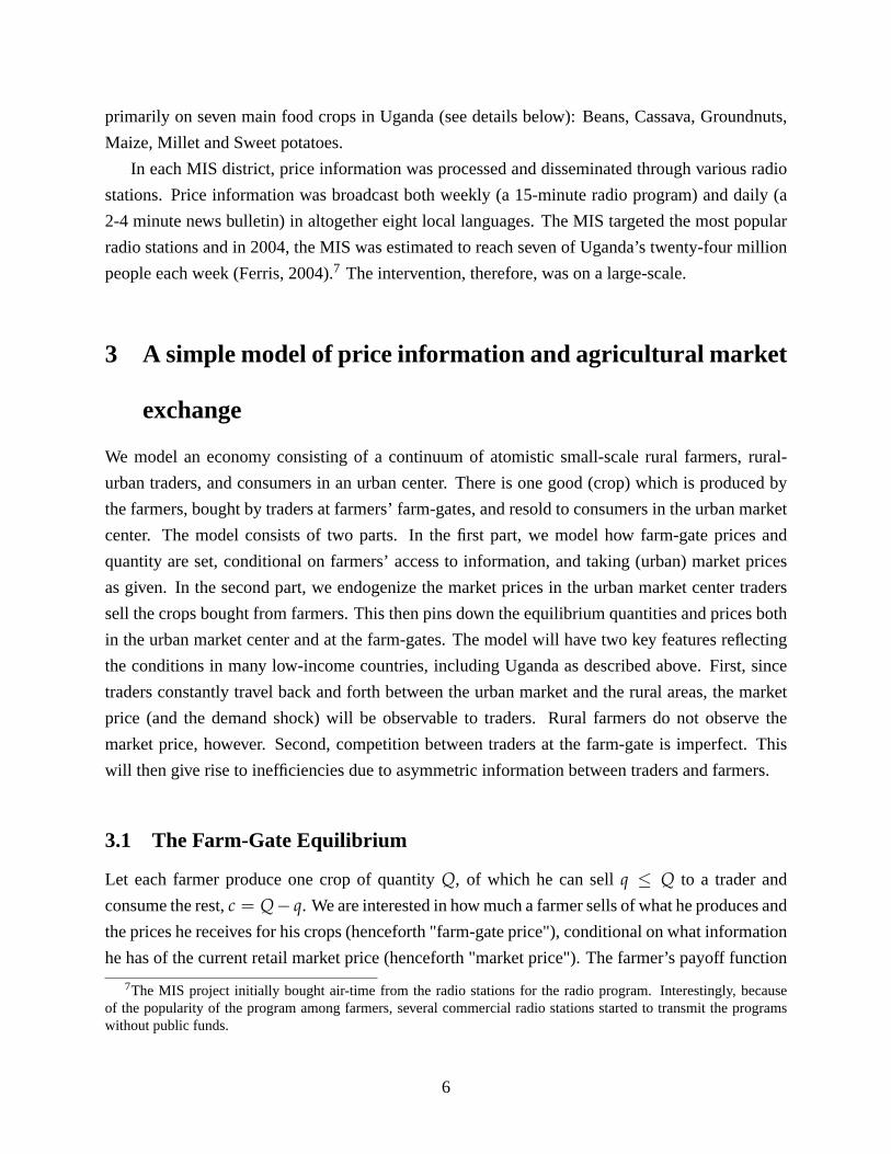
Figure 4 runs a set of placebo regressions similar to column (3), but on using a rolling sam-

ple window mimicing column (3) where instead there are no changes in broadcasts between the

(placebo) pre and post period. The figure include the main specification, at x value equal to zero.

We see that only for the main specification is there an effect.

Together, the results are consistent with prediction 1. Prices decrease when farmers become

informed about the market price, due to a positive supply shock resulting from decreased frictions

between traders and farmers. It is worth noting that it it unlikely that this is the result of a negative

demand shock by urban consumers, since there is little reason for them to decrease demand when

radio is broadcasting price information in the rural areas. Next, we will investigate the supply

shock suggested by Proposition 2 and 3 by using household data directly.

6.2 Farm Gate Outcomes

Table 3 present the results on the extensive margin.

The DDD estimates in columns (1) and (2) are positive (0.103 and 0.089) and significant,

consistent with Prediction 2. Using variation across crops, the DDD estimates in columns (3) and

(4) are also positive and significant. This is true even in the most restrictive specification using

farmer fixed effects (column 4). It is worth pointing out that the estimates in (1)-(4) are also very

21

similar to each other, which is expected but also lends credibility to the identification strategy.

The point estimates imply that farmers that become informed on average increase the likelihood of

selling by approximately 8-10 percentage points. This is substantial, considering that the likelihood

in the sample is about 0.27-0.30.

To assess the identification assumptions, we also run placebo regressions in districts where

there were never any broadcasts (columns 5 and 6), and before there were any broadcasts (columns

7 and 8). None of the DDD estimates are significant and they are close to zero. This lends credi-

bility to the identification strategy.

The DD estimates in columns (1) and (2) are negative (-0.94 and -0.095) and significant, con-

sistent with Prediction 3. Using variation across crops, the DD estimates in columns (3) and (4)

are also negative and significant. In the most restrictive specification using farmer fixed effects, we

see that the coefficient is positive but insignificant. The point estimates imply that farmers that are

uninformed, but live in districts where other farmers become informed, on average decrease the

likelihood of selling by approximately 4-9 percentage points. This is a non-trivial amount. The

placebo regressions in columns (5) - (8) are all insignificant and small or non-negative. Together,

the DD estimates in columns (1) - (8) are consistent with the predictions and indicate that unin-

formed farmers in equlibrium decrease their likelihood of selling to traders, because of negative

price shocks that are the result of positive supply shocks from informed farmers.

Table 4 shows the results for the share of the output sold to the market (and thus not consumed).

We see that the results are in general consistent with Prediction 2 and 3. Overall, the estimates show

a similar pattern as in table 3, there is a positive supply response by informed farmers relative

to uninformed farmers (the DDD estimate is between 0.338 and 0.436), and a negative supply

response by uninformed farmers (the DD estimate is between -0.183 and 0.310). Table 5 estimates

the effect on the farm gate price. The estimates suggest that informed farmers receive relative

higher farm-gate prices than uninformed farmers (the DDD estimate is between 0.149 and 0.385).

There is no robust evidence that the intervention lead uninformed farmers to receive a lower farm-

gate price (the DD estimate is between -0.122 and 0.035). This is consistent with the model, since

the theoretical prediction is ambiguous. The farm-gate price is endogenous to the bargaining with

traders and a price is realized conditional on selling. Since the intervention led the market price to

fall, uninformed farmers decreased market participation. It thus appears that uninformed farmers

only sold their crops when receiving the same farm-gate price as before the intervention. The

placebo regressions in columns 5-8 provide evidence that the effects are not driven by omitted

variables.

Table 6 shows the estimated impact on farmers’ crop incomes. There is a substantial increase in

revenue for informed farmers relative to uninformed farmers. The DDD estimate is between 0.338

and 0.436, implying that the intervention increased informed farmers revenue by 40-55% relative

22

to uninformed farmers. This would be the estimated treatment effect under the partial equilibrium

assumption of unaffected market prices and no negative externalities, since uninformed farmers in

treatment districts would provide the proper counterfactual outcomes. However, this conclusion

is not valid since the intervention was large-scale and lead to general equilibrium effects. The

DD estimate shows the intervention lead to a substantial decrease in crop revenue for uninformed.

The most conservative estimates imply there was a 35-55% reduction in crop revenue for farmers

without access the broadcasts, but living in districts where other farmers did have access. This is

a combination of farm-gate price changes and supply responses, but mainly due to the latter as we

see that the effects on prices are insignificant. The placebo regressions in columns 5-8 show that

there is no evidence that the effects are driven by omitted variables.

The general equilibrium effects on the market prices is driven by the fact that the intervention

was implemented on a large scale, so each districts a large fraction of farmers became better in-

formed. This is also what drives a wedge in farm-gate outcomes between farmers with radio and

farmers without radio in the intervention districts. Table 7 provide additional evidence of the pro-

posed mechanism, as the effects on farm-gate outcomes are more pronounced in districts where a

large share of the population owned a radio before the intervention begun. The signs of the coef-

ficients in columns 1-4 are consistent with the model, although some of the interaction terms are

imprecisely estimated when the variation is at the district level only (the double interaction term).

6.3 Aggregate Impact

The results show that the intervention had distributional consequences: consumers benefited from

lower prices; farmers with access to radio benefited from higher farm revenues, while crop income

fell for farmers without access to radio. To assess the aggregate impact on farm revenue, we

conduct counterfactual calculations. For each observation in the sample of farmers in treatment

districts, and crops that were part of the information campaign, the counterfactual outcomes is

calculated using the DD and DDD coefficients in table 6 (column 3) and calculating what the

revenue would have been in the absence of the intervention. The counterfactual observations are

then summed for the aggregate effects in the (representative) sample. Table 8 shows the results.

The actual total revenue in the sample is 141.2 million Ugandan shillings. The counterfactual

estimate is 144.1 million shillings. The aggregate effect of the intervention is thus negligible (-

2%). This can be compared to the partial equilibrium conclusion that the intervention lead to a

40-55% increase in revenue for farmers with access to the radio (and no effect farmers without

access), which would have been drawn under the partial equilibrium assumption of unaffected

market prices and no negative spillovers on uninformed farmers. Thus, when taking the general

equilibrium effects into account, the interventional had negligible effects on the average farmer

23

incomes, but large distributional consequences.

6.4 Alternative Mechanisms

In this section, we investigate other potential explanations for the results. First, we consider that

the broadcast did not only affect outcome by providing price information. Instead, it may be that

the radio programs also provided farmers with information that had direct effect on agricultural

productivity, by teaching farmers about farming techniques. This could affect quantity sold, quan-

tity produced, as well as the quality of the crops (which could increase the farm-gate price). We use

the UNHS 2005 survey quiz on agricultural technology knowledge to test for the hypothesis that

the broadcast informed farmers about farming technique. Column (1) presents the results using the

fraction of correct answers on the quiz. We find no evidence on technology learning.

Second, we consider the alternative that the price information changed where the farmer sold

their output. In principle, if risk averse farmers become informed about the market price, they may

be more likelihood to travel directly to the district market to sell their crops. Columns (2) - (4)

present the results. We find no evidence of a change in where the goods are sold.26

Finally, we investigate whether the price information made farmers produce more of the crops

for which there was price information. If changing the composition of crops produced is costless

for the farmer (by increasing the plot area for crops with price information and decreasing it for

crops without price information), we would expect output to increase which, in turn, could affect

the farm-gate outcomes. However, unless higher production is also associated with higher share of

output sold, such a production effect would tend to work against finding an effect on s. Columns

(5) - (7) show the results. We find no evidence of production behavior on average.27

7 Concluding Remarks

The paper provides an example where sensible conclusions made in partial equilibrium are offset

by general equilibrium effects. In addition, this paper finds that price information plays an impor-

tant role in facilitating market exchange. The functioning of agricultural markets is central to the

development of low income countries. How to boost agriculture production in developing coun-

tries has been an ongoing policy question. The question is of particular importance for countries in

sub-Saharan Africa where the growth in agricultural yield has been stagnant. While the academic

26We run the same regressions using a dummy indicating if the farmer sold the crops to a private trader in the village.

We find no evidence of changed behavior.27This could be explained either by significant adjustment costs or by beliefs that the price information broadcasts

would terminate. Also, we cannot rule out changes in output within the group MIS crops.

24

literature on the subject is extensive, existing research has primarily focused on two broad sets of

explanations: the low technology adoption rate (of technologies such as HYV crops, irrigation and

fertilizers) and the functioning of agricultural markets.

The issue of functioning markets was a prime concern behind the reforms of the agricultural

markets in many sub-Saharan Africa countries in the late 1980s and 1990s. However, the supply

response from liberalizing agricultural markets has been weaker than expected. One explanation

that has been put forward for this low supply response is that the pre-liberalization period where

the government essentially fixed a price for key food and cash crop commodities (often a price well

below the market price) has been replaced by a situation where better informed (at least about local

market conditions) local traders are able to force down prices to farmers with little idea of price

movements and market trends. Our results are at least qualitatively consistent with this claim.

The effects of information on outcomes are interesting from an economic theory perspective.

However, the effects are also relevant for the discussion about the role of information and com-

munication technologies (ICTs) for economic development (cf. Jensen, 2007). Living standards

for most of the world’s poorest are largely determined on how much they get paid for their output,

mainly crops. Thus, the functioning of output markets is central to the income for farmers en-

gaged in agriculture in low-income countries. In most developing countries, markets are dispersed

and the infrastructure is poor. Small-scale producers typically lack information on market prices,

so that the potential for inefficiency in the allocation of goods across markets and the allocation

between consumption and trading is large.

Moreover, asymmetric information between sellers (i.e. poor small-scale farmers) and buy-

ers adds important distributional concerns. By improving the access to information, ICTs may

help poorly functioning markets work better, improve farmers’ bargaining positions, and thereby

increase the incomes of the poor. In addition, our results suggest that urban consumers, through

lower prices, indirectly benefit from the better functioning. However, access to price information

seldom reaches everyone, and it is still an open question to what extent farmers with little access to

information are affected when a large part of the rural population gets access to good information.

Our results show that price information can have substantial general equilibrium effects, pushing

prices downward. Whether poor farmers without access to information decrease their integration

with markets and become even poorer as a consequence of lower prices is a potentially important

question for future research.

25

8 References

Acemoglu, D., 2010, "Theory, General Equilibrium, and Political Economy in Development Eco-

nomics." Journal of Economic Perspectives, 24(3): 17–32.

Aker, J., 2008, "Does Digital Divide or Provide? The Impact of Cell Phones on Grain Markets

in Niger, Mimeo, University of California, Berkeley.

Banerji, A. and Meenakshi, J.V., 2001, "Competition and Collusion in Grain Markets: Basmati

Auctions in North India", Centre for Development Economics Working Paper 94, University of

Delhi, India.

Baye MR, J. Morgan, 2001, "Information gatekeepers on the Internet and the competitiveness

of homogeneous product markets." American Economic Review, Vol 91(3), p. 454-474.

Baye MR, J. Morgan, and P. Scholten, 2004, "Price dispersion in the small and in the large:

Evidence from an internet price comparison site" Journal of Industrial Economics, Vol 52(4), p.

463-496.

Bolton, P. and M. Dewatripont, 2005, Contract Theory, MIT Press.

Brown JR, A. Goolsbee, 2002, "Does the Internet make markets more competitive? Evidence

from the life insurance industry", Journal of Political Economy, Vol 110(3), p.481-507.

Duflo, E., M. Kremer, and J. Robinson, 2006, "Understanding Technology Adoption: Fertilizer

in Western Kenya, Preliminary Results from Field Experiments," mimeo, MIT.

G. Ellison and S.F. Ellison, 2005, "Lessons About Markets From the Internet", Journal of

Economic Perspectives, Vol. 19(2), p. 139-158.

Ferris, S., 2004, "FOODNET: Information is Changing Things in the Marketplace", ICT Up-

date, Issue 18, CTA, The Netherlands.

Ferris, S. and P. Robbins, 2004, "Developing Marketing Information Services in Eastern Africa:

The FOODNET Experience", International Institute of Tropical Agriculture (IITA), Ibadan, Nige-

ria.

Ferris, S., P. Engoru, and E. Kaganzi, 2008, "Making Market Information Services Work Better

for the Poor in Uganda", CAPRi Working Paper No. 77, International Food Policy Research

Institute, Washington, DC.

Jensen, R. 2007, "The Digital Provide; Information (Technology), Market Performance, and

Welfare in the South Indian Fisheries Sector, The Quarterly Journal of Economics, CXXII (3):

879-924.

Ministry of Finance, 2008, "Uganda Vision 2035", National Planning Authority of the Republic

of Uganda, Kampala.

Mirrlees, J.A., 1971. "An Exploration in the Theory of Optimum Income Taxation," Review of

Economic Studies, vol. 38(114), p. 175-208, April.

26

RATES Center, 2003, "Maize Market Assessment and Baseline Study for Uganda, Center for

Regional Agricultural Trade Expansion Support (RATES Center), Nairobi, Kenya.

Stigler, G., 1961, "The Economics of Information", Journal of Political Economy, 69: 213–225.

Svensson, J. and D. Yanagizawa, 2008, "Tuning in the Market Signal: Contracting and Effi-

ciency under Asymmetric Price Information in Uganda Maize Markets", mimeo, IIES, Stockholm

University.

World Bank, 2007, World Development Report 2008: Agriculture for Development, IBRD,

Washington DC.

27

Appendix

A.1. Details on the propositions

MISPE [x(m)] = E[

xI(m)− xU(m)]

MISIGE [x(m)] = E

[xI(m(r))

]− E

[xU(m(0))

]MISU

GE [x(m)] = E[

xU(m(r))]− E

[xU(m(0))

]∆MISGE [x(m)] = E

[xI(m(r))− xU(m(r))

]Note that MISI

GE = ∆MISGE + MISUGE.

∂MISIGE

∂r;

∂MISUGE

∂r; and

∂∆MISGE

∂r

We summarize the predictions for our main outcome variables: market participation, proxied

by share sold, s(m) = q(m)/Q, the extensive margin ρ, farm-gate prices (p(m)), and market

prices (m), below. All proofs are in appendix.

To arrive at a closed form solution for the market prices, we assume that u(c) is quadratic; i.e.,

u(c) = a(Q− q)− b(Q− q)2.

Taking the total derivative of (26)-(28) with respect to r yields

(38)∂m∗1∂r

= − qI1(m

∗1)

δ+ r ∂qI1(m

∗1)

∂m∗1

< 0

(39)∂m∗2∂r

=qU

2 (m∗2 , m∗3)− qI

1(m∗1)

δ+ r ∂qI1(m

∗2)

∂m∗2+ (1− r) ∂qU

2 (m∗2 ,m∗3)

∂m∗2

< 0

(40)∂m∗3∂r

= 0.

28

The mean market price is

E [m] =3

∑j=1

π jm∗j .

Thus

(A24)∂E [m]

∂r= π1

∂m∗1∂r

+ π2∂m∗2∂r

< 0

For share sold we have

MISUGE

[sU(m)

]=

1Q

E[qU(m∗(r))

]− 1

QE[qU(m∗(0))

]=

1Q

π2

[ρ2(m

∗(r)qU2 (m

∗(r))− ρ2 (m∗(0)) qU

2 (m∗2(0))

]< 0

as ∂qU2 (m

∗(r)) /∂r < 0.

MISIGE

[sI(m)

]=

1Q

E[qI(m∗(r))

]− 1

QE[qU(m∗(0))

]=

1Q

π2

[qI

2(m∗2(r))− ρU

2 (m∗(0)) qU

2 (m∗2(0))

]+

1Q

π3

[ρI

3 (m∗(r)) qI

3(m∗3(r))

]> 0

as qI2 > 1 > qU

2 .

∆MISGE [s(m)] =1Q

E[qI(m(r))

]− 1

QE[qU(m(r))

]=

1Q

π2

[qI

L(m∗2(r))− ρU

2 (m∗(r)) qU

2 (m∗2(r))

]+

1Q

π3

[ρI

3 (m∗(r)) qI

3(m∗3(r))

]> 0

pUL = mL

and

pUH = mH −

qUL

qUH(mH −mL)

29

The first-order conditions for (q1, R1) are

(41)dLdq1

= −π1u′(Q− q1) + λ1m1 − λ2m2 + µm1 = 0

and

(42)dL

dR1= π1 − λ1 + λ2 − µ = 0

The first-order conditions for (q2, R2) are

(43)dLdq2

= −π2u′(Q− q2) + λ2m2 − λ3m3 = 0

and

(44)dL

dR2= π2 − λ2 + λ3 = 0

The first-order conditions for (q3, R3) are

(45)dLdq3

= −π3u′(Q− q3) + λ3m3 = 0

and

(46)dL

dR3= π3 − λ3 = 0

d− δm∗2 + ε2 − rqI2(m

∗2)− (1− r)qU

2 qU2 (m

∗2 , m∗3)

−δ∂m∗2∂r− qI

2 − r∂qI

2∂m∗2

∂m∗2∂r

+ qU2 qU

2 − 2(1− r)qU2

∂qU2

∂m∗2

∂m∗2∂r

∂m∗2∂r

[δ+ r

∂qI2

∂m∗2+ 2(1− r)qU

2∂qU

2∂m∗2

]= qU

2 qU2 − qI

2

30

∂m∗2∂r

=qU

2 qU2 − qI

2[δ+ r ∂qI

2∂m∗2

+ 2(1− r)qU2

∂qU2

∂m∗2

] < 0

(47) d− δm∗1 + ε1 = rqI1(m

∗1)

(48) d− δm∗2 + ε2 = rqI2(m

∗2) + (1− r)ρ2qU

2 (m∗2 , m∗3)

(49) d− δm∗3 + ε3 = qI3(m

∗3)

to

31

Figure 1. Districts with the Market Information Service

Figure 2. The upper panel plots the weekly market price of beans across districts in 2001 (i.e. before the start of broadcasts is most districts). The bottom panel plots the same for millet. The price is in Ugandan shillings. The graphs show that there is substantial price variation across districts at any given point in time, as well as across time within districts.

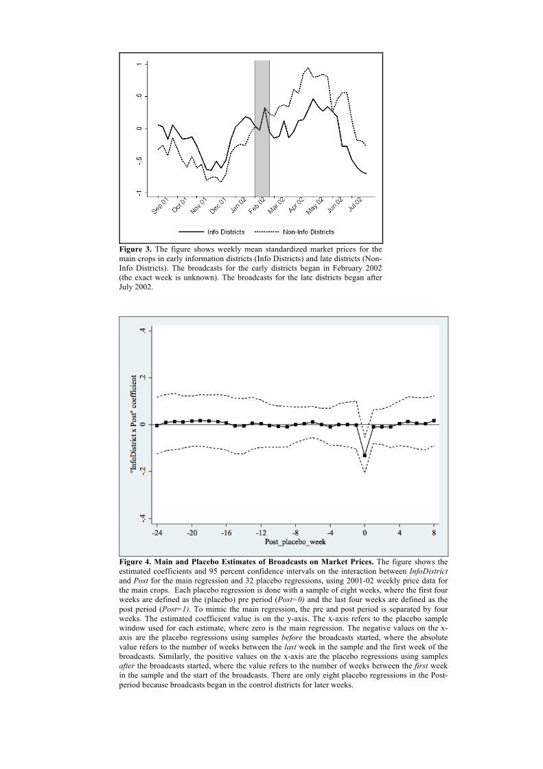
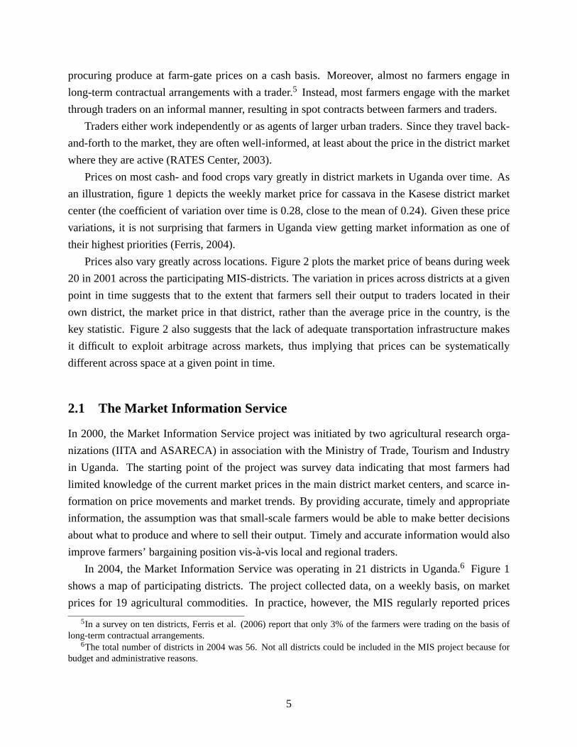
Figure 3. The figure shows weekly mean standardized market prices for the main crops in early information districts (Info Districts) and late districts (Non-Info Districts). The broadcasts for the early districts began in February 2002 (the exact week is unknown). The broadcasts for the late districts began after July 2002.

Figure 4. Main and Placebo Estimates of Broadcasts on Market Prices. The figure shows the estimated coefficients and 95 percent confidence intervals on the interaction between InfoDistrict and Post for the main regression and 32 placebo regressions, using 2001-02 weekly price data for the main crops. Each placebo regression is done with a sample of eight weeks, where the first four weeks are defined as the (placebo) pre period (Post=0) and the last four weeks are defined as the post period (Post=1). To mimic the main regression, the pre and post period is separated by four weeks. The estimated coefficient value is on the y-axis. The x-axis refers to the placebo sample window used for each estimate, where zero is the main regression. The negative values on the x-axis are the placebo regressions using samples before the broadcasts started, where the absolute value refers to the number of weeks between the last week in the sample and the first week of the broadcasts. Similarly, the positive values on the x-axis are the placebo regressions using samples after the broadcasts started, where the value refers to the number of weeks between the first week in the sample and the start of the broadcasts. There are only eight placebo regressions in the Post-period because broadcasts began in the control districts for later weeks.

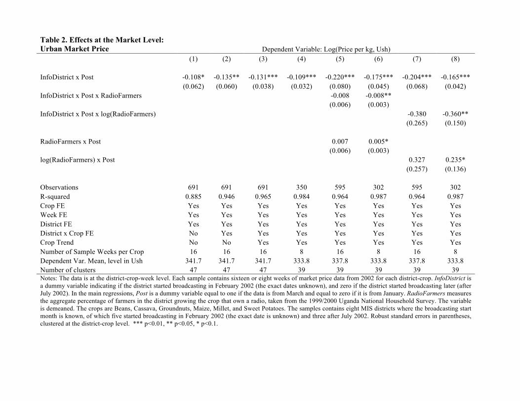
Table 2. Effects at the Market Level: Urban Market Price Dependent Variable: Log(Price per kg, Ush) (1) (2) (3) (4) (5) (6) (7) (8) InfoDistrict x Post -0.108* -0.135** -0.131*** -0.109*** -0.220*** -0.175*** -0.204*** -0.165*** (0.062) (0.060) (0.038) (0.032) (0.080) (0.045) (0.068) (0.042) InfoDistrict x Post x RadioFarmers -0.008 -0.008** (0.006) (0.003) InfoDistrict x Post x log(RadioFarmers) -0.380 -0.360** (0.265) (0.150)

RadioFarmers x Post 0.007 0.005* (0.006) (0.003) log(RadioFarmers) x Post 0.327 0.235* (0.257) (0.136) Observations 691 691 691 350 595 302 595 302 R-squared 0.885 0.946 0.965 0.984 0.964 0.987 0.964 0.987 Crop FE Yes Yes Yes Yes Yes Yes Yes Yes Week FE Yes Yes Yes Yes Yes Yes Yes Yes District FE Yes Yes Yes Yes Yes Yes Yes Yes District x Crop FE No Yes Yes Yes Yes Yes Yes Yes Crop Trend No No Yes Yes Yes Yes Yes Yes Number of Sample Weeks per Crop 16 16 16 8 16 8 16 8 Dependent Var. Mean, level in Ush 341.7 341.7 341.7 333.8 337.8 333.8 337.8 333.8 Number of clusters 47 47 47 39 39 39 39 39 Notes: The data is at the district-crop-week level. Each sample contains sixteen or eight weeks of market price data from 2002 for each district-crop. InfoDistrict is a dummy variable indicating if the district started broadcasting in February 2002 (the exact dates unknown), and zero if the district started broadcasting later (after July 2002). In the main regressions, Post is a dummy variable equal to one if the data is from March and equal to zero if it is from January. RadioFarmers measures the aggregate percentage of farmers in the district growing the crop that own a radio, taken from the 1999/2000 Uganda National Household Survey. The variable is demeaned. The crops are Beans, Cassava, Groundnuts, Maize, Millet, and Sweet Potatoes. The samples contains eight MIS districts where the broadcasting start month is known, of which five started broadcasting in February 2002 (the exact date is unknown) and three after July 2002. Robust standard errors in parentheses, clustered at the district-crop level. *** p<0.01, ** p<0.05, * p<0.1.

Table 3. Effects at the Farm-Gate: Extensive Margin Dependent Variable: Selling any Output, Dummy Main regressions Placebo regressions (1) (2) (3) (4) (5) (6) (7) (8)

InfoCrop x Post x RadioFarmer 0.103** 0.089** 0.003 0.001 (0.042) (0.043) (0.045) (0.046) InfoCrop x Post -0.094** -0.095** -0.002 0.010

(0.039) (0.046) (0.040) (0.045)

InfoCrop x InfoDistrict x RadioFarmer 0.096*** 0.079** 0.004 -0.028 (0.033) (0.039) (0.038) (0.080) InfoCrop x InfoDistrict -0.065** -0.042 0.030 0.084 (0.032) (0.034) (0.055) (0.077)

Observations 23,852 23,852 31,537 31,537 29,362 29,362 21,677 21,677 R-squared 0.113 0.119 0.116 0.363 0.131 0.141 0.150 0.525 Sample Years Pre&Post Pre&Post Post Post Pre&Post Pre&Post Pre Pre Sample Districts Info Info All All Non-Info Non-Info All All Sample Crops All All All All All All All All Crop FE Yes Yes Yes Yes Yes Yes Yes Yes District FE Yes Yes Yes Yes Yes Yes Yes Yes District x Post FE No Yes No No No Yes No No Crop x Season FE No Yes No Yes No Yes No Yes Farmer FE No No No Yes No No No Yes Dependent Variable Mean 0.302 0.302 0.267 0.267 0.285 0.285 0.331 0.331 Notes: InfoCrop indicates that the crop belongs to the crops which the MIS broadcast price information for, and zero otherwise. Post is a dummy variable equal to one if the sample year is 2005 (i.e. after the market information broadcasting started), and zero if it is 1999 (i.e. before the broadcasting started). RadioFarmer is a dummy variable indicating whether the farmer owns a radio. InfoDistrict is a dummy variable indicating if the farmer lives in a MIS district, and zero otherwise. All regressions include a full set of main effects and interaction effects (Results not shown for brevity. The coefficients are in general insignificant). Sample districts equal to All includes both districts with and without the market information service. Selling any Output is a dummy variable indicating if the farmer sold any of the crop output, and zero otherwise. The data is at the plot level, from Uganda National Household Survey. There are two growing seasons per year. Robust standard errors in parentheses, clustered at the district-crop level in regressions 1-2 and 5-6 (there are 17 info districts and 221 district-crop clusters) and clustered at the district level in regressions 3-4 and 7-8 (56 clusters). *** p<0.01, ** p<0.05, * p<0.1.

Table 4. Effects at the Farm-Gate: Share of Output Sold Dependent Variable: Log(Share of the output sold) Main regressions Placebo regressions (1) (2) (3) (4) (5) (6) (7) (8) InfoCrop x Post x RadioFarmer 0.436** 0.393** -0.012 -0.017 (0.183) (0.185) (0.190) (0.193) InfoCrop x Post -0.301* -0.310* 0.045 0.095 (0.163) (0.186) (0.165) (0.179)

InfoCrop x InfoDistrict x RadioFarmer 0.405*** 0.338** -0.021 -0.108 (0.142) (0.164) (0.157) (0.339) InfoCrop x InfoDistrict -0.276** -0.183 0.095 0.276 (0.133) (0.139) (0.204) (0.281) Observations 23,852 23,852 31,537 31,537 29,362 29,362 21,677 21,677 R-squared 0.137 0.143 0.141 0.382 0.160 0.169 0.180 0.549 Sample Years Pre&Post Pre&Post Post Post Pre&Post Pre&Post Pre Pre Sample Districts Info Info All All Non-Info Non-Info All All Sample Crops All All All All All All All All Crop FE Yes Yes Yes Yes Yes Yes Yes Yes District FE Yes Yes Yes Yes Yes Yes Yes Yes District x Post FE No Yes No No No Yes No No Crop x Season FE No Yes No Yes No Yes No Yes Farmer FE No No No Yes No No No Yes Dependent Variable Mean, level 0.168 0.168 0.162 0.162 0.167 0.167 0.176 0.176 Notes: Data definitions and specifications are the same as table 3. Robust standard errors in parentheses, clustered at the district-crop level in regressions 1-2 and 5-6 (there are 17 info districts and 221 district-crop clusters) and clustered at the district level in regressions 3-4 and 7-8 (56 clusters). *** p<0.01, ** p<0.05, * p<0.1.

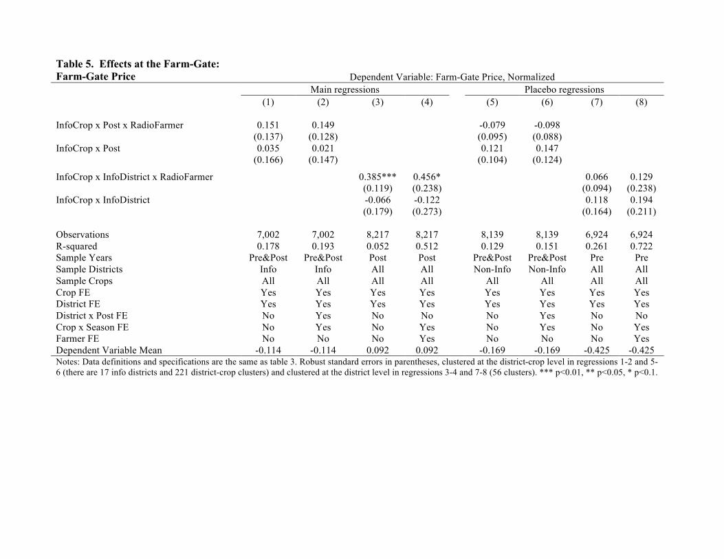
Table 5. Effects at the Farm-Gate: Farm-Gate Price Dependent Variable: Farm-Gate Price, Normalized Main regressions Placebo regressions (1) (2) (3) (4) (5) (6) (7) (8) InfoCrop x Post x RadioFarmer 0.151 0.149 -0.079 -0.098 (0.137) (0.128) (0.095) (0.088) InfoCrop x Post 0.035 0.021 0.121 0.147 (0.166) (0.147) (0.104) (0.124)

InfoCrop x InfoDistrict x RadioFarmer 0.385*** 0.456* 0.066 0.129 (0.119) (0.238) (0.094) (0.238) InfoCrop x InfoDistrict -0.066 -0.122 0.118 0.194 (0.179) (0.273) (0.164) (0.211) Observations 7,002 7,002 8,217 8,217 8,139 8,139 6,924 6,924 R-squared 0.178 0.193 0.052 0.512 0.129 0.151 0.261 0.722 Sample Years Pre&Post Pre&Post Post Post Pre&Post Pre&Post Pre Pre Sample Districts Info Info All All Non-Info Non-Info All All Sample Crops All All All All All All All All Crop FE Yes Yes Yes Yes Yes Yes Yes Yes District FE Yes Yes Yes Yes Yes Yes Yes Yes District x Post FE No Yes No No No Yes No No Crop x Season FE No Yes No Yes No Yes No Yes Farmer FE No No No Yes No No No Yes Dependent Variable Mean -0.114 -0.114 0.092 0.092 -0.169 -0.169 -0.425 -0.425 Notes: Data definitions and specifications are the same as table 3. Robust standard errors in parentheses, clustered at the district-crop level in regressions 1-2 and 5-6 (there are 17 info districts and 221 district-crop clusters) and clustered at the district level in regressions 3-4 and 7-8 (56 clusters). *** p<0.01, ** p<0.05, * p<0.1.

Table 6. Effects at the Farm-Gate: Crop Revenue Dependent Variable: Log(Revenue, Ush) Main regressions Placebo regressions (1) (2) (3) (4) (5) (6) (7) (8) InfoCrop x Post x RadioFarmer 0.627** 0.575** 0.169 0.160 (0.270) (0.270) (0.281) (0.283) InfoCrop x Post -0.768*** -0.781*** -0.285 -0.224 (0.260) (0.284) (0.255) (0.276)

InfoCrop x InfoDistrict x RadioFarmer 0.561** 0.478** 0.086 -0.025 (0.222) (0.236) (0.222) (0.431) InfoCrop x InfoDistrict -0.437** -0.307 0.115 0.404 (0.214) (0.206) (0.268) (0.339) Observations 23,798 23,798 31,490 31,490 29,295 29,295 21,603 21,603 R-squared 0.125 0.131 0.135 0.382 0.143 0.152 0.159 0.540 Sample Years Pre&Post Pre&Post Post Post Pre&Post Pre&Post Pre Pre Sample Districts Info Info All All Non-Info Non-Info All All Sample Crops All All All All All All All All Crop FE Yes Yes Yes Yes Yes Yes Yes Yes District FE Yes Yes Yes Yes Yes Yes Yes Yes District x Post FE No Yes No No No Yes No No Crop x Season FE No Yes No Yes No Yes No Yes Farmer FE No No No Yes No No No Yes Dependent Var. Mean, level in Ush 12145 12145 12694 12694 11149 11149 10104 10104 Notes: Data definitions are the same as table 3. Robust standard errors in parentheses, clustered at the district-crop level in regressions 1-2 and 5-6 (there are 17 info districts and 221 district-crop clusters) and clustered at the district level in regressions 3-4 and 7-8 (56 clusters). *** p<0.01, ** p<0.05, * p<0.1.

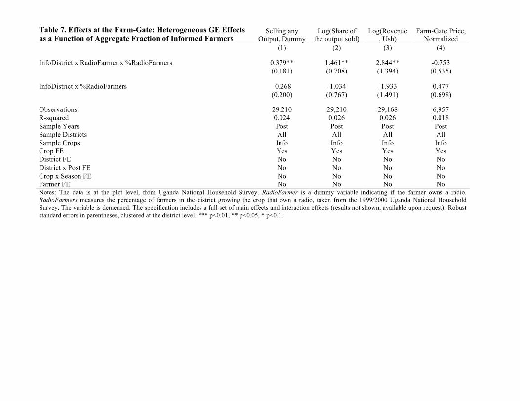
Table 7. Effects at the Farm-Gate: Heterogeneous GE Effects as a Function of Aggregate Fraction of Informed Farmers

Selling any Output, Dummy

Log(Share of the output sold)

Log(Revenue, Ush)

Farm-Gate Price, Normalized

(1) (2) (3) (4)

InfoDistrict x RadioFarmer x %RadioFarmers 0.379** 1.461** 2.844** -0.753

(0.181) (0.708) (1.394) (0.535)

InfoDistrict x %RadioFarmers -0.268 -1.034 -1.933 0.477

(0.200) (0.767) (1.491) (0.698)

Observations 29,210 29,210 29,168 6,957 R-squared 0.024 0.026 0.026 0.018 Sample Years Post Post Post Post Sample Districts All All All All Sample Crops Info Info Info Info Crop FE Yes Yes Yes Yes District FE No No No No District x Post FE No No No No Crop x Season FE No No No No Farmer FE No No No No Notes: The data is at the plot level, from Uganda National Household Survey. RadioFarmer is a dummy variable indicating if the farmer owns a radio. RadioFarmers measures the percentage of farmers in the district growing the crop that own a radio, taken from the 1999/2000 Uganda National Household Survey. The variable is demeaned. The specification includes a full set of main effects and interaction effects (results not shown, available upon request). Robust standard errors in parentheses, clustered at the district level. *** p<0.01, ** p<0.05, * p<0.1.

Table 8. Aggregate Effect on Farmer Income Total crop revenue in

the sample, million Ush Counterfactual total crop

revenue, million Ush Aggregate effect,

million Ush Aggregate effect,

percent

(1) (2) (3) (4)

Informed Farmers 114.7 101.6 13.1 12.9% Uninformed Farmers 26.5 42.5 -16.0 -37.6% Aggregate, Total 141.2 144.1 -2.9 -2.0% Notes: The sample consists of farmers in MIS districts that grow MIS crops. For each farmer-plot observation in the sample, the counterfactuals are calculated using the DD and DDD point estimates and calculating what the revenue would have been in the absence of MIS intervention. The numbers shown for informed and uninformed farmers are the sums when aggregating across all observations within each type of farmer.