Trade and regional inequality - World Banksiteresources.worldbank.org/INTRANETTRADE/Resources/Internal... · inter-regional differences in ... regional inequality, low and medium

1

Trade and regional inequality

Andrés Rodriguez-Pose

1

PRELIMINARY DRAFT – NOT FOR CITATION

Abstract: This paper examines the relationship between openness and within-country

regional inequality across 28 countries over the period 1975-2005, paying special

attention to whether the impact of increases in global trade has affected the developed

and developing world differently. Using a combination of static and dynamic panel

data analysis, it is found that increases in trade have a positive and significant

association with regional inequality. Trade has also had a more polarising effect in

low and middle income countries, whose structural features tend to potentiate the

trade effect and whose levels of internal spatial inequality are, on average,

significantly higher than in high income countries. In particular, states with higher

inter-regional differences in sectoral endowments, lower shares of government

expenditure, and a combination of high internal transaction costs with a higher degree

of coincidence between the regional income distribution and regional foreign market

access positions have experienced the greatest rise in territorial inequality when

exposed to greater trade flows.

Keywords: Trade, regional inequality, low and medium income countries.

1 London School of Economics and Political Science


2

1. Introduction

Recent years have witnessed a surge of scholarly attention on the relationship between

globalisation, the rise of trade, and societal inequality within and across countries.

Most of the work conducted so far has been concerned with the impact of increasing

global market integration on inter-personal income inequality, both in the developed

and the developing world (e.g. Wood, 1994; Ravallion, 2001; Anderson and Nielsen,

2002; Williamson, 2002). The spatial dimension of inequality has attracted far less

attention and the answer to the questions of whether and how increasing and changing

patterns of global market integration are affecting within-country regional disparities

remains very much unanswered. As Kanbur and Venables (2005) underline while

theoretically the relationship between greater openness and spatial inequality remains

ambiguous, the majority of empirical case studies which have dealt with these

questions seem to point towards a positive association between rising regional

inequality and increasing openness, but the direction and dimension of this

relationship is far from uniform and varies from one country to another.

Although the number of single-country case studies which have delved into this

question has grown significantly in recent years, very scant, if any, cross-country

evidence exists unveiling a general causal linkage between greater trade openness and

market integration and intra-national spatial inequality. This may be because,

traditionally, the literature on the evolution of spatial inequalities within countries has

tended – following the path opened by Williamson (1965) in his account of the

relationship between spatial disparities and the stage of economic development – to

focus on the internal and not the external forces of agglomeration and dispersion.


3

From this perspective economic development matters for the evolution of spatial

inequalities, which tend to wane as a country develops. Hence, the factors that matter

in explaining the evolution of regional inequality tend to be internal to the country

itself, while external factors are, at best, regarded as supporting factors in this process.

And when they are taken into consideration, the conclusion is rather inconclusive. As

Milanovic puts it (2005: 428) “country experiences differ and […] openness as such

may not have the same discernable effects on countries regardless of their level of

development, type of economic institutions, and other macroeconomic policies”.

This paper tries to cover this gap in the literature by analysing the relationship

between real trade openness and within-country regional inequality across the world.

It addresses whether a) changes in trade matter for the evolution of spatial inequalities

and b) whether openness to trade affects developed and developing countries

differently. The panel covers the evolution of regional inequality across 28 countries –

including 15 high income and 13 low and medium income countries - over the period

1975-2005.

In order to achieve this, the paper combines the analysis of internal factors – in the

tradition of Williamson – with that of change in real trade as a potential external

factor which may affect the evolution of within-country regional inequality. Internal

factors considered include both Williamson‟s (1965) level of real economic growth

and development, as well as a series of other factors, used as structural conditioning

variables following the new economic geography theory (NEG), which aim to account

for the apparent differences in the relationship between trade openness and spatial

inequality. The analysis is conducted by running unbalanced static panels with


4

country and time fixed effects, followed by a dynamic panel estimation,

differentiating between short-term and long-term effects, as a way to acknowledge

that spatial patterns are bound to be characterised by a high degree of inertia.

The paper is structured into five additional sections. Section 2 introduces a necessarily

brief overview of the existing theoretical and empirical literature. This is followed in

Section 3 by a presentation of the data and its main trends. Section 4 outlines the

theoretical framework and presents the variables included in the analysis, while

Section 5 reports the results of the static and dynamic analysis, distinguishing

between the differential effect of trade on regional inequality in developed and

developing countries, and presents a series of robustness checks. The conclusions are

condensed in Section 6.

2. Trade and regional inequality in the literature

As mentioned in the introduction, the link between changes in trade and the evolution

of regional disparities has hardly captured the imagination of economists and

geographers. In contrast with the spawning literature on trade and interpersonal

inequality, until relatively recently there was indeed a dearth of studies focusing on

the within-country spatial consequences of changes in trade patterns. The emergence

of the NEG theory has somewhat contributed to alleviate this gap in the literature,

especially from a theoretical perspective. A string of NEG models concerned with the

spatial implications of economic openness and trade (e.g. Krugman and Livas-

Elizondo, 1996; Monfort and Nicolini, 2000; Paluzie, 2001; Crozet and Koenig-


5

Soubeyran, 2002; Brülhart et al., 2004) have appeared in recent years. In this

literature the causal effect of globalisation on the national geography of production

and income is conceptualised in terms of changes in cross-border market access that

affect the internal interplay between agglomeration and dispersion forces which, in

turn, determine industrial location dynamics across domestic regions.

Because most of these models have a two-sector nature (agriculture/manufacturing),

the central question has been whether increasing cross-border integration leads to a

greater intra-national concentration of manufacturing activity, and thereby growing

regional inequality. The answer to this question, however, remains far from settled.

Due to the use of different sets of assumptions and of the particular nature of the

agglomeration and dispersion forces included in the models (Brülhart et al., 2004).

contradicting and/or ambiguous conclusions have been derived from this type of

analyses (e.g. Krugman and Livas-Elizondo, 1996 vs. Paluzie, 2001). One of the main

sources of inconclusiveness in the results is that in the existing models increasing

foreign market access gives rise to an ambiguous interplay between export market

supply and demand linkages on one side, versus import competition on the other

(Faber, 2007).

The empirical studies have not been better at resolving this conundrum. Most of the

empirical analyses have tended to concentrate – in part as a result of the scarcity and

lack of reliability of sub-national comparable datasets across countries – on country

case studies as opposed to cross-country analyses. Two countries feature prominently

in empirical approaches. First and foremost post-reform (post-1978) China, where an

expanding number of studies have focused, inter alia, on the trade-to-GDP ratio


6

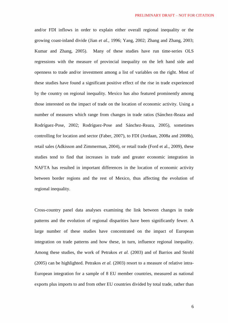
and/or FDI inflows in order to explain either overall regional inequality or the

growing coast-inland divide (Jian et al., 1996; Yang, 2002; Zhang and Zhang, 2003;

Kumar and Zhang, 2005). Many of these studies have run time-series OLS

regressions with the measure of provincial inequality on the left hand side and

openness to trade and/or investment among a list of variables on the right. Most of

these studies have found a significant positive effect of the rise in trade experienced

by the country on regional inequality. Mexico has also featured prominently among

those interested on the impact of trade on the location of economic activity. Using a

number of measures which range from changes in trade ratios (Sánchez-Reaza and

Rodríguez-Pose, 2002; Rodríguez-Pose and Sánchez-Reaza, 2005), sometimes

controlling for location and sector (Faber, 2007), to FDI (Jordaan, 2008a and 2008b),

retail sales (Adkisson and Zimmerman, 2004), or retail trade (Ford et al., 2009), these

studies tend to find that increases in trade and greater economic integration in

NAFTA has resulted in important differences in the location of economic activity

between border regions and the rest of Mexico, thus affecting the evolution of

regional inequality.

Cross-country panel data analyses examining the link between changes in trade

patterns and the evolution of regional disparities have been significantly fewer. A

large number of these studies have concentrated on the impact of European

integration on trade patterns and how these, in turn, influence regional inequality.

Among these studies, the work of Petrakos et al. (2003) and of Barrios and Strobl

(2005) can be highlighted. Petrakos et al. (2003) resort to a measure of relative intra-

European integration for a sample of 8 EU member countries, measured as national

exports plus imports to and from other EU countries divided by total trade, rather than


7

the overall trade-to-GDP ratios. Running a system of seemingly unrelated equations,

they find mixed explanatory results for this variable and conclude that the effect of

European integration affects countries differently. Barrios and Strobl (2005) run fixed

effects OLS analyses for the EU15 over the period 1975-2000. They aim to explain

how a measure of regional inequalities within each country is influenced by the trade-

to-GDP ratio, as well as by trade over GDP in PPP terms. For the latter, they find a

significant positive effect on regional inequalities among EU15 countries over 1975-

2000.

The studies which have focused on this topic including a more varied number of

countries – involving both developed and developing ones – are rarer. Among these,

the work of Milanovic (2005) and Rodríguez-Pose and Gill (2006) stand out.

Milanovic (2005) addresses the evolution of regional inequalities across the five most

populous countries of the world: China, India, the US, Indonesia, and Brazil over

varying time spans during the period 1980-2000. The results of his static fixed effects

and dynamic Arellano-Bover panel analyses point to an absence of a significant

causal relationship between openness and regional inequalities. Rodríguez-Pose and

Gill (2006) map two sets of binary relationships – first between nominal trade

openness and regional inequality, and second between a trade composition index and

regional inequality – four eight countries, including Brazil, China, Germany, India,

Italy, Mexico, Spain, and the US, over varying time spans between 1970-2000. They

conclude that it is not trade openness per se which has any bearing on the evolution of

regional inequality, but its combination with the evolution of the manufacturing-to-

agriculture share of exports which influences which regions gain and which lose from

greater economic integration over time. They find indicative support for this


8

hypothesis based on the coincidence between changes in of the evolution of their

trade composition index and changes in regional inequalities across countries.

Given the diversity of results in both theoretical and empirical analyses, one would be

hard pressed to generalise from the existing literature. The relationship between trade

and regional inequalities thus remains wide open, both from a theoretical and

empirical perspective.

3. Overall trade and regional inequality: Empirical evidence.

This paper revisits the question of the link between trade and regional inequality,

using an unbalanced panel dataset comprising 28 countries over the period 1975-

2005. The 28 countries included in the analysis are presented in Table 1, which

groups them according to whether they have experienced increasing or decreasing

spatial disparities over the indicated time span covered by the data.

Table 1: Increasing versus Decreasing Regional Inequality

Increasing Regional Inequality Decreasing Regional Inequality

Australia (1990-2005) Austria (1988-2004)

Bulgaria (1995-2004) Belgium (1977-1996)

China (1978-2004) Brazil (1989-2004)

Czech Republic (1995-2004) Canada (1981-2005)

Finland (1995-2004) France (1982-2004)

Greece (1979-2004) Italy (1995-2004)

Hungary (1995-2004) Japan (1975-2004)

India (1993-2002) Netherlands (1986-2004)

Indonesia (2000-2005) South Africa (1995-2005)

Mexico (1993-2004)

Poland (1995-2004)

Portugal (1995-2004)

Romania (1998-2004)

Slovak Republic (1995-2004)

Spain (1980-2004)

Sweden (1994-2004)

Thailand (1994-2005)


9

UK (1994-2004)

USA (1975-2005)

As can be seen, the majority of the countries included in the sample have experienced

a rise in regional disparities over the period of analysis. In 19 out of the 28 countries

spatial inequalities have increased, while only nine countries have experienced a

decrease in inequalities. The rate of change varies enormously across countries.

Countries such as Bulgaria, China, Hungary, India, Poland, Romania or the Slovak

Republic have witnessed a very rapid rise in disparities, while the rate of increase has

been more moderate in places such as Australia, Spain, the UK, or the US. Rates of

decline in inequalities have also varied hugely, with Belgium and Brazil experiencing

the strongest decline in territorial inequalities. There is also no apparent difference

between the trajectories of developed and of emerging countries. Some of the low and

medium income countries included in the sample have seen spatial disparities increase

– e.g. Bulgaria, China, India, Indonesia, Mexico, Thailand – while the opposite have

been true in Brazil and South Africa.

The primary question asked is whether any general relationship between the evolution

of trade openness and spatial inequalities that holds across different types of countries

can be detected. In order to assess whether this is the case, a simple binary association

between yearly measures of real trade openness and regional inequality for each

country separately is performed. Figure 1 maps the regression coefficient of the log

Gini index of regional GDP per capita on the log of the share of exports plus imports

in GDP adjusted to purchasing power parities (PPP) by country. In Figure 2 the same

regression coefficients are presented, having replaced the annual measures by three-


10

-1

-0.8

-0.6

-0.4

-0.2

0

0.2

0.4

0.6

0.8

Fin

lan

d

Ca

na

da

Ne

the

rla

nd

s

Ja

pa

n

Au

str

ia

Sw

ed

en

Be

lgiu

m

Fra

nc

e

US

Bra

zil

Ita

ly

Po

rtu

ga

l

Au

str

ali

a

Me

xic

o

Sp

ain

Ind

on

es

ia

So

uth

Afr

ica

Slo

va

k R

ep

Th

ail

an

d

Ch

ina

Po

lan

d

Bu

lgari

a

UK

Hu

ng

ary

Ind

ia

Ro

ma

nia

Gre

ec

e

Cze

ch

Re

p

Inequality-Openness Coeffients

Inequality-Openness Coef. 3-year Averages

-3

-2

-1

0

1

2

3

4

5

6

Sw

ed

en

Fin

lan

d

Ca

na

da

Au

str

alia

Ne

the

rla

nd

s

Ja

pa

n

Po

rtu

ga

l

US

Be

lgiu

m

Fra

nc

e

UK

Bra

zil

Me

xic

o

Sp

ain

Ind

on

es

ia

Au

str

ia

Slo

va

k R

ep

Bu

lga

ria

Ch

ina

Th

aila

nd

Gre

ec

e

So

uth

Hu

ng

ary

Ita

ly

Po

lan

d

Ro

ma

nia

Cze

ch

Re

p

Ind

ia

year averages, as multiannual averages may be better than yearly data at picking up

any potential lagged effects, thus correcting for yearly fluctuations.

Figure 1: Regression Coefficients of Regional Inequality on Real Trade

Openness

Figure 2: Regression Coefficients of Regional Inequality on Openness for 3-year

averages


11

The Figures show no dominating pattern. There is a huge diversity in both the sign

and the dimension of the coefficient, with some countries sporting a positive

relationship between trade and the evolution of regional disparities and others a

negative one. There consequently seems to be, as indicated by Milanovic (2005) and

Rodríguez-Pose and Gill (2006) no evidence of the presence of a simple linear

relationship between the two variables that holds across countries. A more subtle

observation concerns the sequence of countries from left to right. On the whole,

wealthier countries (Finland, Sweden, Canada, Netherlands, Japan) tend to be located

on the left-hand side of both figures, displaying a negative association between

increases in trade and regional disparities, while poorer countries tend to be found

towards the right-hand side of the figure (India, Romania, Poland). This relationship

is, however, far from linear, with some high and middle income countries (Spain,

Italy, South Korea, UK, Greece) displaying a positive binary association between

trade and spatial inequality.

4. Model and data

There are limitations in what can be inferred from the above simple binary

associations, as they only offer very limited information about the mechanisms at play

and many other factors may be affecting the evolution of within-country regional

disparities. In order to address this issue, in the following paragraphs I formulate a

formal econometric specification with additional controls and conditioning variables

aimed at testing whether there is a significant association between openness and


12

spatial inequality and whether this association – if it exists – affects developed and

developing countries in a different way.

4.1. The basic model

With very few exceptions (e.g. Milanovic, 2005), the bulk of studies on the

determinants of regional inequalities are based on static one-yearly specifications.

However, regional inequality is bound to be a time-persistent phenomenon with a

high degree of inertia. This makes overlooking time considerations problematic.

Theory, however, provides no clear (if any) insights concerning the temporal

dimension of internal spatial adjustments to changes in external market access. Hence,

rather than guessing an appropriate adjustment timeframe, the paper tackles potential

inertia is by formulating a dynamic model with past levels of spatial inequality on the

dependent variable side. The use of dynamic panels – complementing static panels –

has the advantage of introducing the distinction between short term and long term

effects.

Taken this into consideration, the following general model is formulated:

Giniit = α + ∑βxit + εit (1)

Where Giniit is the level of inequality in country i at time t corresponding to the

spatial configuration that would arise if there was no inertia in the system and xit is a

vector of independent variables conditioning the spatial distribution of income in any

given country i at time t. Using Brown‟s (1952) classical habit persistence model,

equation (1) is transformed into equation (2):


13

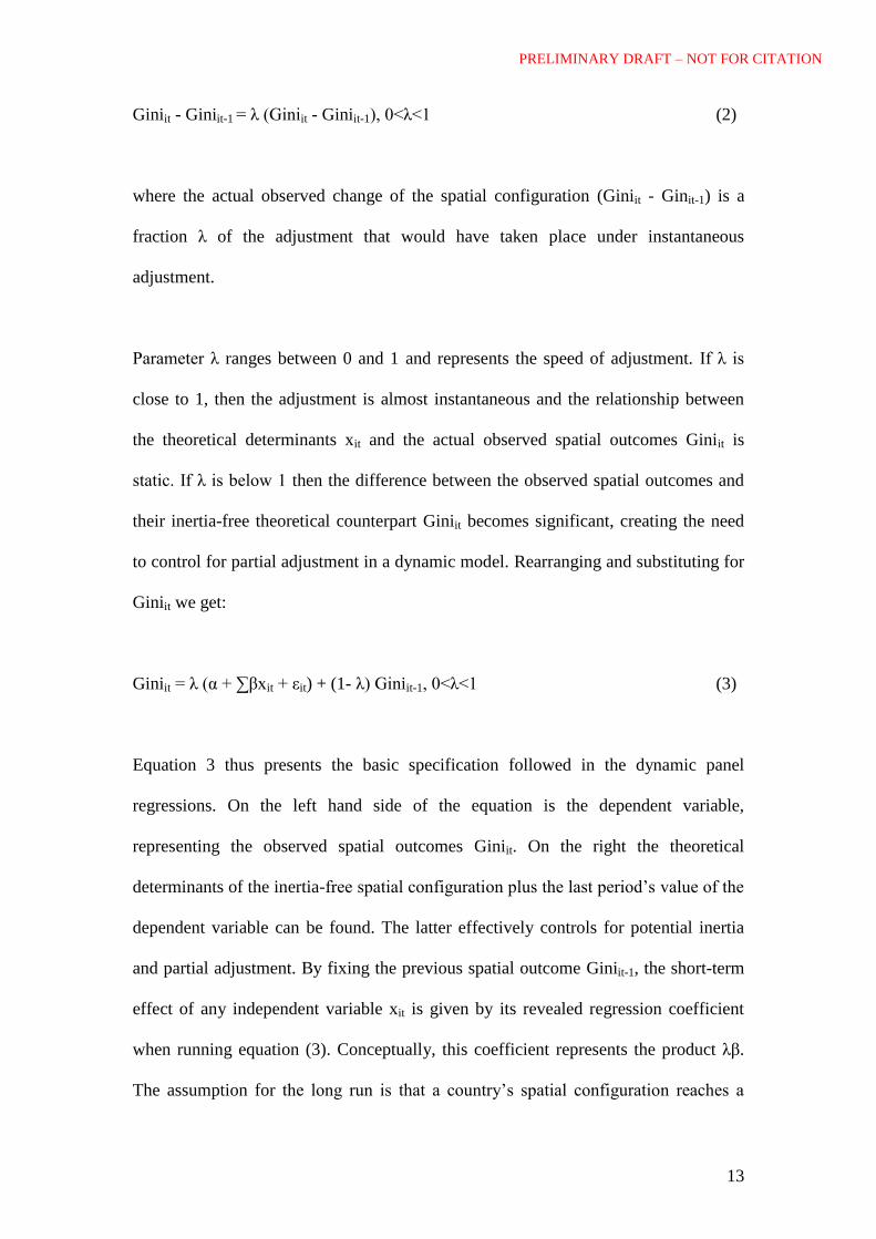
Giniit - Giniit-1 = λ (Giniit - Giniit-1), 0<λ<1 (2)

where the actual observed change of the spatial configuration (Giniit - Ginit-1) is a

fraction λ of the adjustment that would have taken place under instantaneous

adjustment.

Parameter λ ranges between 0 and 1 and represents the speed of adjustment. If λ is

close to 1, then the adjustment is almost instantaneous and the relationship between

the theoretical determinants xit and the actual observed spatial outcomes Giniit is

static. If λ is below 1 then the difference between the observed spatial outcomes and

their inertia-free theoretical counterpart Giniit becomes significant, creating the need

to control for partial adjustment in a dynamic model. Rearranging and substituting for

Giniit we get:

Giniit = λ (α + ∑βxit + εit) + (1- λ) Giniit-1, 0<λ<1 (3)

Equation 3 thus presents the basic specification followed in the dynamic panel

regressions. On the left hand side of the equation is the dependent variable,

representing the observed spatial outcomes Giniit. On the right the theoretical

determinants of the inertia-free spatial configuration plus the last period‟s value of the

dependent variable can be found. The latter effectively controls for potential inertia

and partial adjustment. By fixing the previous spatial outcome Giniit-1, the short-term

effect of any independent variable xit is given by its revealed regression coefficient

when running equation (3). Conceptually, this coefficient represents the product λβ.

The assumption for the long run is that a country‟s spatial configuration reaches a


14

more or less stable equilibrium so that current and past year‟s inequality levels are

close to identical. Setting Giniit-1 equal to Giniit in equation 3, the long-term effect of

any independent variable on the spatial configuration can thus be derived by dividing

the observed regression coefficient λβ by the speed of adjustment parameter λ. One

can thus obtain the long-term effects by dividing the coefficients of the independent

variables by 1 minus the coefficient of the lagged dependent variable.

4.2. The conditioning variables

Having set the basic model, the task now is to identify an appropriate set of

conditioning variables capturing the relationship between trade openness and internal

spatial inequality in the form of equation 1. This is done in two stages: the first one

drawing on recent NEG models, and the second reaching beyond the purely market

access driven framework.

In an NEG core-periphery framework and as a consequence of NEG‟s basic two

sector assumption and of the absence of intermediate supply linkages, foreign

manufacturing enters as a source of competition, while foreign agriculture becomes

the single source of external market access (Brülhart et al., 2004). This makes

distinguishing whether or not high foreign market access in a setting of market

integration becomes good or bad for regional growth difficult and inversely related to

the relative size of the foreign manufacturing sector.

There is therefore a need to consider cross-border intermediate supply linkages and a

multi-sector industrial scenario in order to overcome this ambiguity (Faber, 2007).


15

This gives rise to an additional pull factor towards high market access regions once

trade is liberalised and allows export market potential, intermediate supply potential,

and import competition to affect domestic sectors differently, depending on the

comparative advantages revealed by market integration. Sectors characterised by a

revealed comparative advantage and/or cross-border intermediate supply linkages will

grow faster in regions with good foreign market access, whereas import competing

sectors gain in relative terms in regions with higher „natural protection‟ from poor

market access. Faber (2007) finds empirical support for this trade-location linkage

across 43 industrial sectors in post-NAFTA Mexico over the period 1993-2003.

The implications of this possible divergence of sectoral location patterns under cross-

border market integration are important for understanding whether and how market

accessibility affects regional performance. Regions with high relative foreign market

access that attract the winners of integration will also tend to shed declining sectors,

hence resulting in medium to long-term above-average regional growth rates than

regions with limited and/or constrained foreign market access.

In conditions of increasing trade and economic integration two additional important

country factors may play an important conditioning role in determining the evolution

of regional inequalities. First is the degree of variation of foreign market accessibility

among regions within any given country. If, given the discussion above, we assume

that high relative foreign market access drives regional attractiveness for expanding

sectors, then the locational pull will be strongest in countries that are characterised by

high regional differences in cross-border market accessibility. The strength of this

factor is further conditioned by the degree of coincidence between the existing


16

regional income distribution and the distribution of relative foreign market access.

When relatively wealthy regions are also those with a greater degree of accessibility,

increases in trade are likely to exacerbate previously existing inequalities. In contrast,

when poorer regions have a market accessibility advantage relative to better off

regions, the net outcome of increases in trade is likely to be a reduction in regional

disparities and within-country territorial convergence. Hence, it can be safely assumed

that greater trade openness will have a more polarising effect in countries

characterised by a) higher differences in foreign market accessibility among its

regions and b) where there is also a high degree of coincidence between the regional

income distribution and accessibility to foreign markets.

Stepping outside the NEG framework, other factors may come into play in

determining the link between trade and regional inequality. Among these factors

differences in the distribution of human capital and skills and infrastructure would

certainly affect trade patterns as well as economic growth. It can therefore be

envisaged that the spatial impact of greater trade openness is likely to be more severe

in countries exhibiting higher regional differences endowments and sectoral

specialisation.

The role of government policies may also enhance or attenuate the spatial effects of

changes in trade patterns. Governments with a greater redistributive capacity through

public policies will tend to counter any potential tendency of increases in trade

patterns leading to greater geographical polarisation. Budgetary or regional policy

transfers from prosperous to lagging regions will thus counter rises in regional

inequality, making the effect of trade openness on spatial inequality likely to be more


17

severe in countries with a weaker redistributive capacity by the central government

and/or with fewer provisions for interregional transfers.

A fourth conditioning factor concerns the degree of labour mobility, especially

within-country mobility. It can be envisaged that a higher inter-regional mobility of

workers will offset increases in regional per capita inequality (Puga, 1997). Hence,

the effect of trade on regional inequality will be more severe in countries with a lower

degree of inter-regional labour mobility.

Unfortunately, due to lack of comparable and reliable data on inter-regional labour

mobility across the 28 countries covered in the analysis, this hypothesis cannot be

tested. We therefore have to assume that labour mobility is not systematically

correlated with any of the other included regressors, implying that there is no omitted

variable problem in leaving out this conditioning interaction.

There is also a need to control for the possibility of omitted variables which may

affect the relationship between trade and spatial inequality. The key element in this

real relates to Williamson‟s (1965) classical account of the linkage between spatial

disparities and the stage of economic development. In this account, the level of

within-country spatial inequalities is fundamentally the result of the level of national

economic development (proxied in this case by real GDP per capita and its growth).

As countries prosper the level of within-country regional inequalities tends to

diminish, making economic growth a primary driver of changes in spatial inequalities.

As economic growth is also likely to be correlated with changes in trade (Sachs and


18

Warner, 1995), a control for real GDP per capita and its interaction with the country‟s

development stage is included in the analysis.

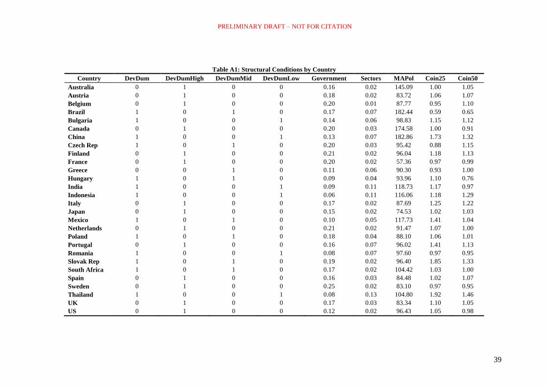
4.3. The empirical model, data and method

The above discussion leads to the transformation of equation (1) by the following

empirical specification (4). Table A1 in the appendix presents the actual values of the

structural conditions across the 28 countries.

ln Inequalityit = α + β1 [ln(GDPcapit) * Developmenti] + β2 [ln(Tradeit) *

ln(MarketAccessi) * ln(Coincidencei)] + β3 [ln(Trade/GDPit) * ln(Sectorsi)] + β4

[ln(Trade/GDPit) * ln(Governmenti)] + εit (4)

where:

Ineqiit represents the level of within-country regional inequality in country i in year t,

measured using the Gini index of regional GDP per capita.

GDPcapit denotes real GDP per capita in PPP constant US$ (2000) for country i in

year t.

Developmenti is a dummy variable which takes the value of 1 if country i is

developing or transition economy and 0 otherwise. The categories were assigned on

the basis of historical World Bank classifications. Each country was assigned to its


19

most frequent classification over the time period covered in the dataset. This variable

is, in turn, subdivided into three components:

a) High incomei is another dummy variable which takes the value of 1 if country i

has been most frequently classified as high income country and 0 otherwise.

b) Middle incomei is a dummy variable which takes the value 1 of if country i has

been most frequently classified as middle income country and 0 otherwise.

c) Low incomei is a dummy variable which takes the value of 1 if country i has

been most frequently classified as low income country and 0 otherwise.

Tradeit represents the total Imports and exports in current US$ divided by GDP in PPP

current US$ for country i in year t.

Sectorsi is a variable aimed at capturing the degree of inter-regional sectoral

differences that exist in different countries, proxied by the standard deviation of the

share of agriculture in regional GDP across domestic regions, averaged across time

periods under study for country i. Ideally a finer sectoral disaggregation in order to

capture in a more precise way the variation of modern sector endowments between

domestic regions should have been used. But given the diversity of countries included

in the panel, the share of agriculture in regional GDPs over time was the best

comparable indicator available.

Governmenti denotes the size of government in country i, captured by the share of

non-military/non-defence government expenditure in total GDP averaged across time

periods under study. It is assumed that inter-regional transfer programmes and social


20

expenditures are linearly related to the level of non-military government expenditure

in total GDP.

MarketAccessi denotes the degree of inter-regional differences in foreign market

access across countries. Taking into account existing data constraints in the countries

covered in the sample, two alternative measures of market access are used. The first

variable (Surfacei) is each country‟s surface area in square kilometres. However, the

surface area of a country is a rather crude measure of market access, especially in

view of the huge diversity in population density among countries. Hence an

alternative composite measure of internal market access polarisation

(MAPolaristaioni) is constructed. In this measure the surface area in square kilometres

of a country is transformed into an index ranging between 0 and 100 and introduced

as the first element. The second element is the population density adjusted ratio of

paved road and railway kilometres over the square root of the land area. The

adjustment for population density is intended to account for the fact that some

countries have vast unpopulated zones while others are much more densely populated.

The infrastructure-to-land area ratio is weighted by transforming each country‟s land

area to the panel‟s mean population density. This adjustment implies that in the case

of Australia this greatly reduces its adjusted land area, whereas in the case of the

Netherlands it increases it. The paved road and railroad line kilometres relative to the

square root of the adjusted land area is used as a population-density adjusted indicator

of infrastructure quantity and quality across countries. As with the surface area, this

composite measure is transformed into an index ranging between 0 and 100 where

100 represents the score for the country with the lowest endowment in infrastructure

(in our panel Thailand, see table A1). The two 0-100 scores are then combined into an


21

aggregate score of possible values between 0-200, where increasing scores suggest

increasing internal differences of foreign market access.

The main logic behind the use of the MAPolaristaioni variable is that both the level of

absolute internal distances (element 1) and the population density adjusted

infrastructural endowments (element 2) determine the degree of inter-regional

variation in access to foreign markets. The first concerns the internal transport

distances, the second proxies for the average transportation costs of a country. A one-

to-one weighting was chosen under the assumption that the proxy for quality and

quantity of transport infrastructure will not only reflect average transport costs per km

of landmass, but also the number and availability of international transhipment and

customs facilities along a country‟s coasts and borders.

Coincidencei reflects the degree of coincidence between relative regional market

access positions and regional income per capita levels across countries. Once again,

two alternative measures of coincidence between both factors are used. The first

(Coincidence25i) is the ratio of the average GDP per capita levels of the regions in the

top 25 percent in terms of foreign market access over average regional GDP per

capita. The second (Coincidence50i) calculates the same ratio on the basis of the

regions in the top 50 percent in terms of relative foreign market access. In order to

insure consistency with the dependent measure of regional inequality which treats

each region as one observation, the coincidence ratios are also computed disregarding

regional population sizes.


22

The question is of course how to determine relative market access positions. In the

absence of adequate and comparable datasets of regional transport costs to an

equivalent selection of international trade points in each country, the method used

consists in first identifying the trade entry points accountable for at least 70% of the

country‟s total trade, as well as the top quarter or half of the regions in terms of border

or coast location in closest proximity to the main trade routes. In the cases where two

regions were very close in terms of border/coast accessibility to the main trade routes,

the region with the higher number of international ports or border crossings was

chosen.

Beyond a mere response to limited data availability, this geography based

construction of the coincidence measures also addresses a potential endogeneity issue.

Assuming that perfect data about each region‟s foreign market access in terms of

actual transport cost weighted market potential was available, it would be highly

likely that high degrees of regional inequality would be associated to higher degrees

of coincidence, because regional prosperity tends to be a driver of market access when

measured in terms of human-built infrastructure. Relying on physical proximity and

border or coast location instead is not subject to this potential endogeneity issue. As in

the case of the previous structural conditioning variables, the coincidence measures

were averaged across periods for each country.

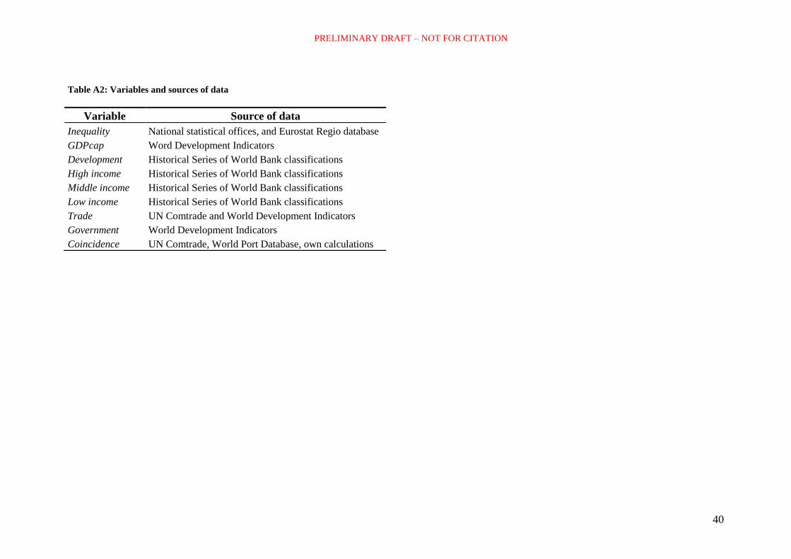
The data sources for each of the variables are presented in Table A2 in Appendix.

Finally ε represents the error term.


23

In order to assess whether trade and the remaining variables included under equation

(4) affect regional inequalities, both static OLS with country and time fixed effects, as

well as dynamic panels are run. In the case of the dynamic regressions, general

method of moments (GMM) estimation following Arellano and Bond (1991),

Arellano and Bover (1995), and Blundell and Bond (1998) are applied. The problem

with running OLS on panels that include the lagged dependent variable is that it will

be correlated with the error term even after getting rid of the unobserved country

heterogeneity therein. To adjust for this bias, Arellano and Bond have proposed a first

difference GMM estimator that uses lagged values of the dependent and

predetermined variables and differences of the strictly exogenous ones as instruments.

Arellano and Bover and Blundell and Bond have proposed a system GMM estimator

in which variables in levels are instrumented with lags of their own first differences to

exploit additional moment conditions.

5. The impact of trade on regional inequality

In this section the results of running the different specifications of equation (4) are

presented. Table 2 introduces the results for the static OLS with country and time

fixed effects. Given that all unobserved invariant country and time heterogeneity has

been eliminated from the model, the coefficients can be interpreted as the partial

effects that annual variations of independent variables around the country mean have

had on annual variations of spatial inequality around the country mean.

INSERT TABLE 2 HERE.


24

The results of the static panel highlight, in contrast to most previous studies operating

with international panels, the presence of a weak, but positive and highly significant

effect of the dimension of real trade on spatial inequality when pooling across all

countries. Having controlled for the internal growth effect and its different slope

across developed and developing countries, a one percent increase in real trade

openness is on average associated with a 0.17 percent increase of the Gini index of

regional inequality (Table 2, Regression 1). The results also indicate that this effect is

significantly stronger in developing countries than in developed ones (Table 2,

Regression 2), although the binary Development dummy interaction is only significant

at the 10 percent level.

Regressions 3 to 8 take us beyond the simple binary relationship between trade and

inequality and introduce the conditioning structural variables identified in the

previous section. All the coefficients have the expected sign – rises in trade are

associated with lower regional inequalities in countries with large government size

and with higher inequalities in cases of strong inter-regional sectoral differences,

when there are important differences in market access and when these coincide with

geographical disparities in income per capita - and, with the exception of one

particular combination of the spatial structure conditions in regression 5, all are

significant at the one percent level. Poorer countries with lower government

expenditure, higher variations in regional sectoral structures, and a spatial structure

dominated by high internal transaction costs coupled with a higher degree of

coincidence between prosperous regions and foreign market access are thus bound to

experience greater rises in regional inequality when opening to foreign trade.


25

Interestingly, when all conditioning interactions are added together (Regression 9,

Table 2), the binary Development dummy interaction effect becomes insignificant.

The same is the case for the Government expenditure interaction. These changes

could simply be the result of collinearity between the Development dummy and the

Government variable. But this is not the case. The Government variable remains

significant once the Sectors interaction is dropped, meaning that the problem of

collinearity arises between the Government and Sectors interactions, but not between

Development and Government. This suggests that the proposed structural variables

account to a great extent for the apparent differences in the association between trade

and within-country spatial inequalities across developed and developing countries.

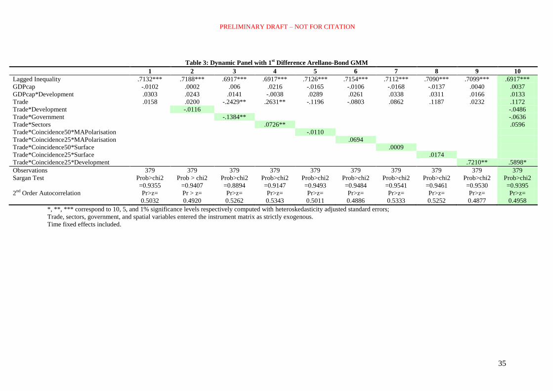
Table 3 presents the results of the dynamic panel regressions. The results were

computed using the xtabond2 command in STATA (Roodman, 2006). Reported

results correspond to the 1st difference Arellano-Bond GMM estimation. The reason

for this is that the usually preferred Arellano-Bover system GMM was repeatedly

rejected by the Sargan test of over-identification, indicating that its additional

assumptions on the data generating process did not hold.


As could be expected, when switching to dynamic panels with the lagged level of

inequality included on the right hand side, most of the differences in current within-

country spatial inequality levels are explained by previous levels of within-country

inequality, meaning also that the effect of trade openness on regional inequality


26

ceases to hold (Table 3, Regression 1). The same is the case for the binary

Development dummy interaction term in Regression 2 (Table 3).

Regressions 3 to 9 introduce the structural conditions in the dynamic model. Here, the

partial effects of the static fixed effect model are confirmed in the cases of sectoral

differences and government expenditure, which also render the Trade variable

significant at the five percent level (Regressions 3 and 4, Table 3). The introduction of

the spatial variables, in contrast, while keeping the same coefficient signs of the static

analysis, display insignificant coefficients with the exception of Regression 9 which

substitutes the Development dummy by a relatively crude binary proxy of internal

market access polarisation.

The high degree of inertia inferred from the coefficient of the lagged level of regional

inequality comes as no surprise, with the speed of adjustment parameter lying around

0.3, which suggest the presence of a strong difference between short term and long

term effects of all included independent factors (Table 3).

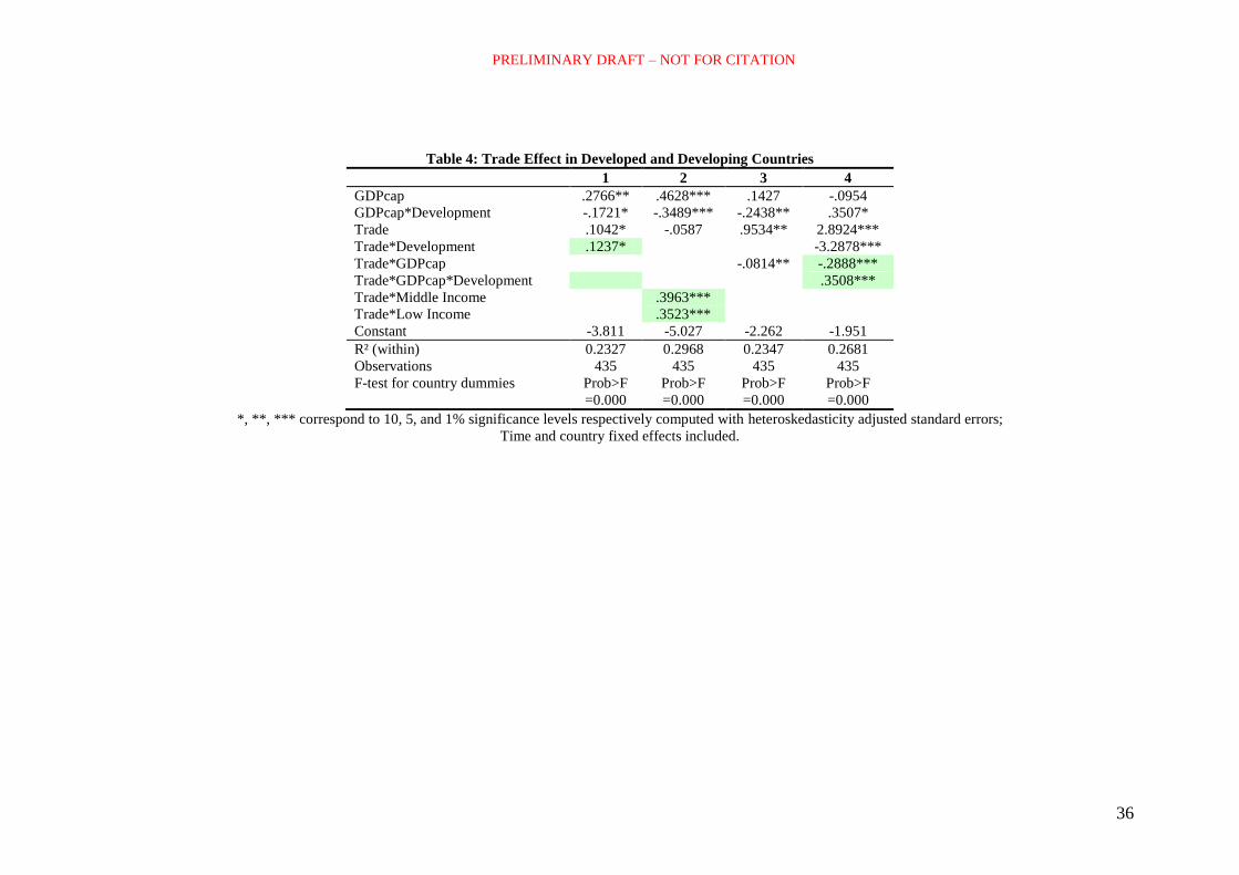
5.1. Differences between developed and developing countries

In order to test whether the weak binary Development dummy interaction of the trade

impact also holds at a less aggregate categorical level, the panel is divided into high

middle and low income countries, according to the World Bank‟s classification, using

the high income group as the reference category. Table 4 reports the results of this

type of analysis.


27

Adding greater nuances to the developed/developing country division leads to an

increase in the significance of development dummy interactions (Regression 2, Table

4), in comparison to those reported in Regression 2 (Table 2). The data suggest that

variations in levels of trade openness have a significantly higher association with

average variations in spatial inequality in middle and low income countries than in

high income ones. There is, in contrast, no significant difference between the impact

of changes in trade on spatial inequality between low and middle income countries

(Regression 2, Table 4).


When instead of testing for different slopes of the trade effect on spatial inequality

across groups, we examine whether the effect of trade has changed as countries

progress in terms of economic development – by interacting trade openness with the

countries‟ real GDP per capita (Regression 3, Table 4) – the resulting coefficient

points towards a weakening of the positive association between increases in trade and

within-country spatial inequalities as countries become wealthier. Overall, Table 4

suggests that trade has had a higher impact on spatial inequality in developing

countries, and that this effect tends to be diminishing with economic development at a

slower pace than in developed countries.

An important final point concerns the striking difference between the coefficient

results for the internal determinant of spatial inequality in the tradition of Williamson,

and the external trade induced factor that was the focus of this study. Particularly


28

surprising is the negative and frequently significant coefficient of the interaction term.

This suggests that, after controlling for real trade openness, variations of real income

per capita have on average had a less positive association to variations in spatial

inequality in developing countries as opposed to developed ones. In other words,

economic growth has on average been less polarising in developing countries than in

developed ones.

These findings indicate that the external effect of real trade openness on internal

spatial inequality appears to have had a more polarising effect in developing countries

than economic growth. The important question in this context is of course what the

underlying structural factors are behind the difference of the trade effect. As noted in

Regression 9 in Table 2 above, the diminishing size and lack of significance of the

development dummy interaction after controlling for spatial structure, government

intervention, and sectoral differences point to these structural factors as part of the

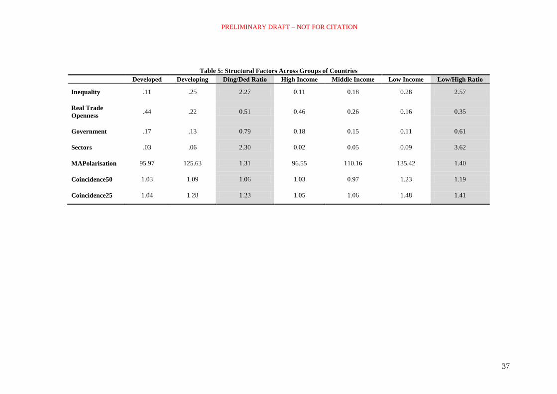
reason. This line of reasoning is confirmed in Table 5 in which the variable averages

are collapsed across different country groups.


In Table 5 all the identified conditioning country characteristics appear to be working

against developing countries. This is especially pronounced after disaggregating

countries into high middle and low income clusters, especially when taking into

account current existing degrees of global integration, on one side, and levels of

spatial inequality, on the other. This implies that, as highlighted by Rodríguez-Pose

and Gill (2006), the room for growth in spatial inequalities is much greater in the


29

developing than in the developed world as a) developing countries tend to be

characterised by structural features that potentiate the polarising effect of trade

openness, b) they already have much higher existing levels of spatial inequality, and

c) their level of trade openness is, on average, still only a fraction of the one among

developed countries.

In order to check whether these results are robust to differences in specifications, the

Gini index of regional inequality is replaced with alternative inequality measures. The

specifications in Tables 2 to 4 are thus run replacing Gini coefficient of within-

country regional inequality as the dependent variable with the Theil index. The results

are robust to the change in specification and can be provided upon request.

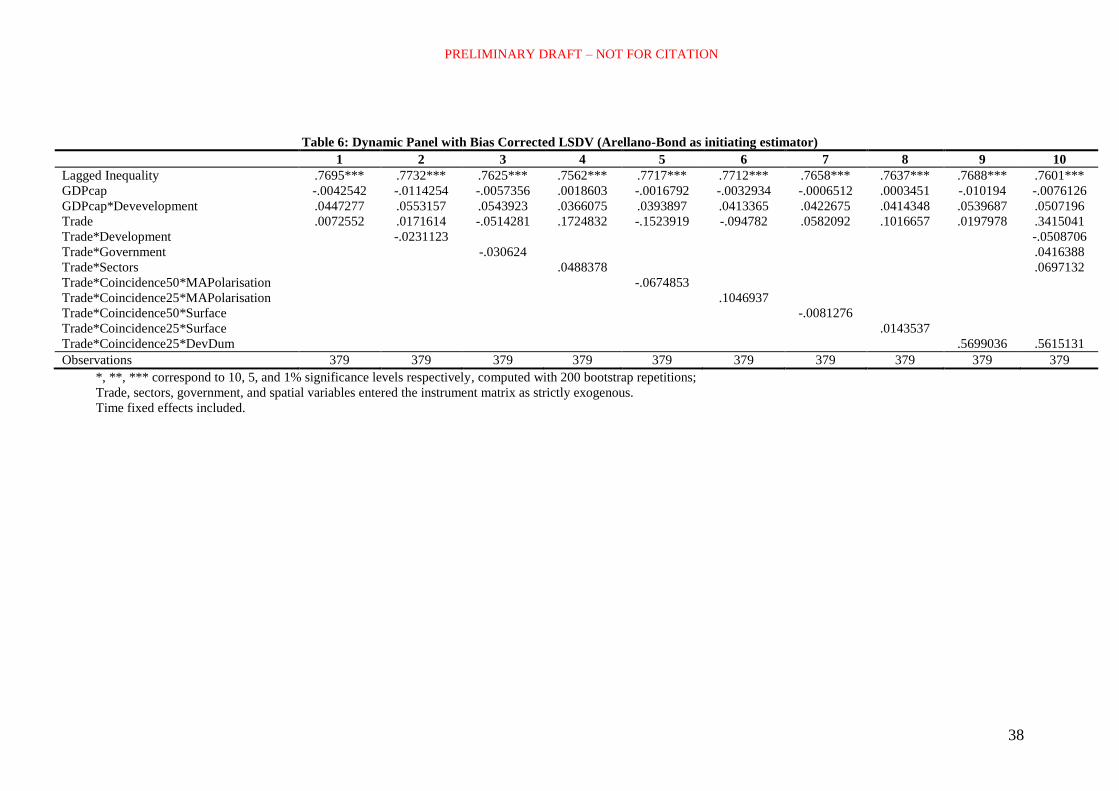
Another robustness check, given the limited number of observations in a panel

including 28 countries relative to the time of the analysis, is to use a bias-corrected

least squares dummy variable (LSDV) estimator (Kiviet, 1995; Bun and Kiviet,

2003), instead of a instrumental variable GMM estimation. This approach also allows

to accommodate for unbalanced panels (Bruno, 2005). By resorting to this method,

the aim is to check whether the results from the Arellano-Bond GMM estimation in

Table 3 prove robust to an alternative estimator. The results are displayed in Table 6.

Standard errors have been derived by setting the number of bootstrap repetitions to

200.



30

Table 6 reveals that the size and sign of the coefficients of interest remain similar to

those presented in Table 3. The speed of adjustment parameter slightly decreases to

below 0.25 as indicated by the higher coefficient of the lagged level of regional

inequality. However, none of the previously found significance levels is confirmed.

This makes it difficult to draw any firm conclusions on the dynamic adjustment

process between openness and regional inequality from our data. Beyond the highly

significant static associations that we found, the data do not support any robust partial

relationship in the dynamic setting that introduces short term and long term effects.

6. Conclusion

The aim of this paper has been to improve our understanding of the relationship

between changes in trade patterns linked to global market integration, on the one

hand, and within-country spatial inequalities, on the other, both from a theoretical and

an empirical perspective.

The paper is based on a model which combines spatial characteristics with a series of

additional country features. The spatial characteristics include the degree of inter-

regional variation in access to foreign markets and whether these differences in

foreign markets coincide with differences in income. The conditioning country

features include the degree of inter-regional sectoral variation, the level of

government expenditure, and the degree of labour mobility. Lack of data on the latter

allows us to test for the former two conditions only. In the theoretical tradition of

Williamson (1965), the paper also controls for the internal growth effect and its


31

interaction with the country‟s development stage. The influence of these variables on

the evolution of within-country regional inequality is then tested using both static

fixed effects, as well as dynamic panels.

The results show that trade matters for the evolution of regional inequalities. There is

a weak but significant association between both factors in static panel analyses, which

improves as the conditioning variables are included in the analysis. This implies that,

while changes in trade make a difference for the evolution of spatial disparities, the

impact of changes in trade is more polarising in countries with higher inter-regional

sectoral differences, lower shares of non-military government expenditure, and a

combination of higher internal transaction costs with higher degrees of coincidence

between wealthier regions and foreign market access. However, the spatial country

variables cease to be significant once controlling for lagged levels of inequality in

dynamic panels, meaning that no firm conclusions can be extracted regarding the

dynamic timeframe of spatial adjustments and the distinction between short term and

long term effects of trade openness.

The key result is that changes in trade patters seem to affect the evolution of regional

inequality in developing countries to a much greater extent than in developed ones.

The spatially polarising effect of trade also decreases at a significantly slower pace in

developing countries than in developed ones. And trade, in contrast to what was

suggested by Williamson (1965), seems to have a greater sway on the evolution of

regional inequality than economic growth. This means that economic growth –

whether directly provoked by changes in trade or not – cannot offset the potentially

negative effects for territorial equality of increases in trade in the developing world.


32

By and large, countries in the developing world are characterised by a series of

features that are likely to potentiate the spatially polarising effects of greater openness

to trade. Their higher existing levels of regional inequality, their greater degree of

sectoral polarisation, the fact that their wealthier regions often coincide with the key

entry points to trade, and their weaker state will contribute to exacerbate regional

disparities as trade with the external world increases. And countries in the developing

world have a much greater scope for increases in spatial polarisation, as their level of

international market integration, while growing rapidly, is still a fraction of that of

developed countries.

Policy-makers in the developing world – as well as international organisations – may

thus need to tread carefully when thinking about the potential implications of greater

market openness for their countries. While greater openness to trade is likely to yield

rewards in terms of growth and the absolute welfare of local citizens, it may also

bring the unwelcome consequence of greater territorial polarisation. While this may

not necessarily be bad in the short term, enhancing territorial inequality in countries

with already high levels of spatial polarisation and where territorial differences may

pile on top of pre-existent social, cultural, ethnic, and/or religious grievances, can

contribute flare up tensions which could ultimately undermine the very economic

benefits that trade is suppose to bring about. Hence, the territorial implications of

trade need to be brought into the trade policy equation, if the potential economic

benefits of greater openness to trade for countries in the developing world are to be

preserved.


33

References

To be added


34

– Figures and Tables –

Table 2: Static Panel with Country and Time Fixed Effects

1 2 3 4 5 6 7 8 9

GDPcap .2433** .2766** .2657** .3049*** .1799 .1791 .2251** .2418** .3607***

GDPcap*Development -.1223 -.1721 -.1523* -.1992** -.0540 -.0404 -.1025 -.0998 -.2363***

Trade .1728*** .1042* -.4840*** .8620*** 1.7055*** 1.770*** 1.1955** 1.2968*** 2.1162***

Trade*Development .1237* .1160

Trade*Government -.3337*** -.0932

Trade*Sectors .2081*** .2358***

Trade*Coincidence50*MAPolarisation .7888

Trade*Coincidence25*MAPolarisation .8889***

Trade*Coincidence50*Surface .1544***

Trade*Coincidence25*Surface .1351*** .1272**

Constant -3.631 -3.811 -3.729 -3.968 -3.297 -3.317 -3.699 -3.841 -4.592

R² (within) 0.227 0.2327 0.2527 0.2577 0.2503 0.2622 0.2775 0.2885 0.359

Observations 435 435 435 435 435 435 435 435 435

F-test for country dummies Prob>F

=0.000

Prob>F

=0.000

Prob>F

=0.000

Prob>F

=0.000

Prob>F

=0.000

Prob>F

=0.000

Prob>F

=0.000

Prob>F

=0.000

Prob>F

=0.000

*, **, *** correspond to 10, 5, and 1% significance levels respectively computed with heteroskedasticity adjusted standard errors;

Time and country fixed effects included.


35

Table 3: Dynamic Panel with 1st Difference Arellano-Bond GMM

1 2 3 4 5 6 7 8 9 10

Lagged Inequality .7132*** .7188*** .6917*** .6917*** .7126*** .7154*** .7112*** .7090*** .7099*** .6917***

GDPcap -.0102 .0002 .006 .0216 -.0165 -.0106 -.0168 -.0137 .0040 .0037

GDPcap*Development .0303 .0243 .0141 -.0038 .0289 .0261 .0338 .0311 .0166 .0133

Trade .0158 .0200 -.2429** .2631** -.1196 -.0803 .0862 .1187 .0232 .1172

Trade*Development -.0116 -.0486

Trade*Government -.1384** -.0636

Trade*Sectors .0726** .0596

Trade*Coincidence50*MAPolarisation -.0110


Trade*Coincidence50*Surface .0009


Trade*Coincidence25*Development .7210** .5898*

Observations 379 379 379 379 379 379 379 379 379 379

Sargan Test

Prob>chi2

=0.9355

Prob > chi2

=0.9407

Prob>chi2

=0.8894

Prob>chi2

=0.9147

Prob>chi2

=0.9493

Prob>chi2

=0.9484

Prob>chi2

=0.9541

Prob>chi2

=0.9461

Prob>chi2

=0.9530

Prob>chi2

=0.9395

2nd

Order Autocorrelation

Pr>z=

0.5032

Pr > z=

0.4920

Pr>z=

0.5262

Pr>z=

0.5343

Pr>z=

0.5011

Pr>z=

0.4886

Pr>z=

0.5333

Pr>z=

0.5252

Pr>z=

0.4877

Pr>z=

0.4958


Trade, sectors, government, and spatial variables entered the instrument matrix as strictly exogenous.

Time fixed effects included.


36

Table 4: Trade Effect in Developed and Developing Countries

1 2 3 4

GDPcap .2766** .4628*** .1427 -.0954

GDPcap*Development -.1721* -.3489*** -.2438** .3507*

Trade .1042* -.0587 .9534** 2.8924***

Trade*Development .1237* -3.2878***

Trade*GDPcap -.0814** -.2888***

Trade*GDPcap*Development .3508***

Trade*Middle Income .3963***

Trade*Low Income .3523***

Constant -3.811 -5.027 -2.262 -1.951

R² (within) 0.2327 0.2968 0.2347 0.2681

Observations 435 435 435 435

F-test for country dummies Prob>F

=0.000

Prob>F

=0.000

Prob>F

=0.000

Prob>F

=0.000


Time and country fixed effects included.


37

Table 5: Structural Factors Across Groups of Countries

Developed Developing Ding/Ded Ratio High Income Middle Income Low Income Low/High Ratio

Inequality .11 .25 2.27 0.11 0.18 0.28 2.57

Real Trade

Openness .44 .22 0.51 0.46 0.26 0.16 0.35

Government .17 .13 0.79 0.18 0.15 0.11 0.61

Sectors .03 .06 2.30 0.02 0.05 0.09 3.62

MAPolarisation 95.97 125.63 1.31 96.55 110.16 135.42 1.40

Coincidence50 1.03 1.09 1.06 1.03 0.97 1.23 1.19

Coincidence25 1.04 1.28 1.23 1.05 1.06 1.48 1.41


38

Table 6: Dynamic Panel with Bias Corrected LSDV (Arellano-Bond as initiating estimator)

1 2 3 4 5 6 7 8 9 10

Lagged Inequality .7695*** .7732*** .7625*** .7562*** .7717*** .7712*** .7658*** .7637*** .7688*** .7601***

GDPcap -.0042542 -.0114254 -.0057356 .0018603 -.0016792 -.0032934 -.0006512 .0003451 -.010194 -.0076126

GDPcap*Devevelopment .0447277 .0553157 .0543923 .0366075 .0393897 .0413365 .0422675 .0414348 .0539687 .0507196

Trade .0072552 .0171614 -.0514281 .1724832 -.1523919 -.094782 .0582092 .1016657 .0197978 .3415041

Trade*Development -.0231123 -.0508706

Trade*Government -.030624 .0416388

Trade*Sectors .0488378 .0697132

Trade*Coincidence50*MAPolarisation -.0674853


Trade*Coincidence50*Surface -.0081276


Trade*Coincidence25*DevDum .5699036 .5615131

Observations 379 379 379 379 379 379 379 379 379 379 *, **, *** correspond to 10, 5, and 1% significance levels respectively, computed with 200 bootstrap repetitions;

Trade, sectors, government, and spatial variables entered the instrument matrix as strictly exogenous.

Time fixed effects included.


39

Table A1: Structural Conditions by Country

Country DevDum DevDumHigh DevDumMid DevDumLow Government Sectors MAPol Coin25 Coin50

Australia 0 1 0 0 0.16 0.02 145.09 1.00 1.05

Austria 0 1 0 0 0.18 0.02 83.72 1.06 1.07

Belgium 0 1 0 0 0.20 0.01 87.77 0.95 1.10

Brazil 1 0 1 0 0.17 0.07 182.44 0.59 0.65

Bulgaria 1 0 0 1 0.14 0.06 98.83 1.15 1.12

Canada 0 1 0 0 0.20 0.03 174.58 1.00 0.91

China 1 0 0 1 0.13 0.07 182.86 1.73 1.32

Czech Rep 1 0 1 0 0.20 0.03 95.42 0.88 1.15

Finland 0 1 0 0 0.21 0.02 96.04 1.18 1.13

France 0 1 0 0 0.20 0.02 57.36 0.97 0.99

Greece 0 0 1 0 0.11 0.06 90.30 0.93 1.00

Hungary 1 0 1 0 0.09 0.04 93.96 1.10 0.76

India 1 0 0 1 0.09 0.11 118.73 1.17 0.97

Indonesia 1 0 0 1 0.06 0.11 116.06 1.18 1.29

Italy 0 1 0 0 0.17 0.02 87.69 1.25 1.22

Japan 0 1 0 0 0.15 0.02 74.53 1.02 1.03

Mexico 1 0 1 0 0.10 0.05 117.73 1.41 1.04

Netherlands 0 1 0 0 0.21 0.02 91.47 1.07 1.00

Poland 1 0 1 0 0.18 0.04 88.10 1.06 1.01

Portugal 0 1 0 0 0.16 0.07 96.02 1.41 1.13

Romania 1 0 0 1 0.08 0.07 97.60 0.97 0.95

Slovak Rep 1 0 1 0 0.19 0.02 96.40 1.85 1.33

South Africa 1 0 1 0 0.17 0.02 104.42 1.03 1.00

Spain 0 1 0 0 0.16 0.03 84.48 1.02 1.07

Sweden 0 1 0 0 0.25 0.02 83.10 0.97 0.95

Thailand 1 0 0 1 0.08 0.13 104.80 1.92 1.46

UK 0 1 0 0 0.17 0.03 83.34 1.10 1.05

US 0 1 0 0 0.12 0.02 96.43 1.05 0.98


40

Table A2: Variables and sources of data

Variable Source of data

Inequality National statistical offices, and Eurostat Regio database

GDPcap Word Development Indicators

Development Historical Series of World Bank classifications

High income Historical Series of World Bank classifications

Middle income Historical Series of World Bank classifications

Low income Historical Series of World Bank classifications

Trade UN Comtrade and World Development Indicators

Government World Development Indicators

Coincidence UN Comtrade, World Port Database, own calculations

Documents

Trade and regional inequality - World Banksiteresources.worldbank.org/INTRANETTRADE/Resources/Internal... · inter-regional differences in ... regional inequality, low and medium