Tracking down European Markets

Tracking Performance of ETFs and Mutual Index Funds

Authors: Andrii Antonov Tobias Schirra

Supervisor: Catherine Lions

Student

Umeå School of Business and Economics

Spring semester 2013

Master thesis, two-year, 30 hp

Summary In recent years, the financial service industry demonstrated substantial growth of Exchange Traded Funds (ETFs). Apart from offering access to new and more specific investment opportunities, many ETFs enter direct competition with conventional, already existing Mutual Index Funds. With 22,1% growth of assets over the past 5 years, the European market by now accounts for 19% of the global ETF market, while at the same time we observe a decline of cash flows to Mutual Index Funds.

Given the recent development, index investors are likely to face a choice between ETFs and Mutual Index Funds offering the same service. The purpose of this study is to analyze those two similar investment instruments towards the quality of achieving their objective, which is to deliver a performance as close as possible to the respective benchmarks'. The analysis will be performed for the European market, i.e. we include only Index Funds that track European indices.

This study is guided by objectivism and positivism as ontological and epistemological positions. We conduct a deductive research by reviewing and testing previous findings through the formulation of hypotheses that serve our purpose. For our analysis we gather quantitative data in the form of daily prices for 21 ETFs and 22 Mutual Index Funds, tracking 9 European indices. We further use a time frame of 7 years (2006-2012), which we analyze as a whole as well as divided into sub-periods as determined by different states of the European market. As a basis for the analysis we calculate return differences and different measures of tracking risk.

Our results show that on average ETFs as well as Mutual Index Funds sufficiently replicate index performance with approximately the same level of tracking risk for both instruments. Furthermore, we see no significant impact of expected returns or index volatility on return difference. However, through examination of fees and tracking errors during recent economic turmoils, we show that ETFs first bear lower directly attributed costs and second are less affected by down markets than Mutual Funds (MFs).

Keywords: Mutual index funds, exchange traded funds, tracking error, index replication, European index funds.

i

Acknowledgment

Our deep gratitude goes to our supervisor Catherine Lions who guided us through the entire process by sharing with us her extensive experience and knowledge about academic writing in general and about the requirements of Umeå School of Business in particular. Her preparative advice at the beginning of this work, as well as invaluable feedback throughout the different development stages were material to keep this thesis on track and provided us with constructive guideposts.

We further express our gratitude to Anja Baumeister and Priyantha Wijayatunga. Anja for sparing no effort when using her advanced linguistic skills to provide us with great advice on how to give this work a final linguistic polish. Priyantha for giving us technical advice for our analysis, and with his expertise helped us to enhance our statistical understanding.

Last but not least we thank our families, companions and friends for their motivating support throughout this sometimes rather exhausting period. You helped us clear our minds and to restock energy to continue.

Thank You!

Umeå, May 24, 2013

Tobias Schirra Andrii Antonov

tobias.schirra001@gmail.com s1mple@bigmir.net

ii

Table of Contents Summary ............................................................................................................................ i Acknowledgment .............................................................................................................. ii Table of Contents ............................................................................................................ iii List of Tables ................................................................................................................... vi Table of Figures ............................................................................................................... vi Table of Equations .......................................................................................................... vii Table of Abbreviations .................................................................................................. viii 1. Introduction .................................................................................................................. 1

1.1. Problem Background ............................................................................................. 1

1.2. Research Question ................................................................................................. 3

1.3. Research Purpose ................................................................................................... 3

1.4. Research Gap and Contribution ............................................................................. 4

1.5. Delimitations ......................................................................................................... 5

1.6. Structure and Disposition of the Research ............................................................ 6

1.7. Important Definitions ............................................................................................ 8

2. Theoretical Methodology ............................................................................................. 9

2.1. Pre-understanding .................................................................................................. 9

2.2. Research Philosophy ........................................................................................... 10

2.2.1. Ontology ........................................................................................................... 10

2.2.2. Epistemology .................................................................................................... 11

2.2.3. Paradigm ........................................................................................................... 12

2.3. Research Approach .............................................................................................. 13

2.4. Research Method ................................................................................................. 14

2.5. Choice of Literature and Critical Assessment ..................................................... 15

2.5.1. Choice of Sources ............................................................................................. 16

2.5.2. Data Type ......................................................................................................... 17

2.5.3. Quality Assessment of Sources ........................................................................ 17

2.6. Ethical Considerations ......................................................................................... 18

2.7. Summary of Methodological Choices ................................................................. 19

3. Theoretical Framework............................................................................................... 20

3.1. Index .................................................................................................................... 20

3.1.1. Definition and Use of an Index......................................................................... 20

3.1.2. Index Calculation .............................................................................................. 21

3.1.3. Index Specifics: The Example of the S&P 500 ................................................ 25

3.2. Return, Risk and Error ......................................................................................... 25

3.2.1. Return Difference ............................................................................................. 25

iii

3.2.2. Tracking Risk ................................................................................................... 26

3.3. Funds ................................................................................................................... 27

3.3.1. UITs, Open-end and Closed-end Funds ........................................................... 27

3.3.2. Exchange Traded Funds ................................................................................... 28

3.4. Fund Management ............................................................................................... 30

3.4.1. Active and Passive Management ...................................................................... 30

3.4.2. Passive Index Tracking ..................................................................................... 31

3.4.3. Index Tracking Strategy ................................................................................... 32

3.4.3.1. Physical Replication ...................................................................................... 32

3.4.3.2. Synthetic Replication ..................................................................................... 33

3.4.4. Fund Related Costs ........................................................................................... 35

3.5. Structural Summary of Theoretical Framework .................................................. 36

3.6. Review of Previous Literature ............................................................................. 36

3.6.1. ETFs vs. Mutual Index Funds .......................................................................... 36

3.5.2 Tracking Quality and Market Condition ........................................................... 39

3.6. Formulation of Hypotheses ................................................................................. 40

4. Practical Methodology ................................................................................................ 43

4.1. Data Collection .................................................................................................... 43

4.1.1. Sampling Method ............................................................................................. 43

4.1.2. Selection Criteria .............................................................................................. 44

4.1.3. Data Selection ................................................................................................... 45

4.1.4. MSCI Europe .................................................................................................... 47

4.1.5. Time Horizon .................................................................................................... 47

4.1.6. Sub-Periods ....................................................................................................... 48

4.2. Data Treatment and Adjustment .......................................................................... 49

4.3. Statistics ............................................................................................................... 50

4.3.1. Statistical Expression of Hypotheses ................................................................ 50

4.3.2. Calculating Returns .......................................................................................... 51

4.3.3. Volatility ........................................................................................................... 52

4.3.4. Correlation Analysis ......................................................................................... 52

4.3.5. Regression Analysis ......................................................................................... 53

4.3.6. Tracking Error Estimates .................................................................................. 54

4.3.7. Two-Sample t-test ............................................................................................ 55

4.4. Regressions with categorical dependent variable ................................................ 56

4.4.1. Linear Probability Model (LPM) ...................................................................... 56

4.4.2. Probit model ..................................................................................................... 57

4.4.3. Logit model ...................................................................................................... 57

iv

4.5. Measurement Quality .......................................................................................... 59

4.5.1. Reliability ......................................................................................................... 59

4.5.2. Validity ............................................................................................................. 60

4.5.3. Generalizability ................................................................................................ 60

5. Results and Analysis ................................................................................................... 61

5.1. Chapter Outline ................................................................................................... 61

5.2. Comprehensive Descriptive Statistics ................................................................. 62

5.3. Analysis of return differences.............................................................................. 63

5.3.1. Summary of Results: Logistic regression ......................................................... 64

5.4. Tracking Error Analysis ...................................................................................... 65

5.4.1. Regression and Tracking Error 1 ...................................................................... 65

5.4.2. Long Term comparison of Tracking Errors ...................................................... 68

5.4.3. Annual Comparison of Tracking Errors ........................................................... 70

5.4.4. Market State and Tracking Error ...................................................................... 75

5.5. Total Expense Ratio ............................................................................................ 78

5.5.1. ETF vs. MIF ..................................................................................................... 78

5.5.2. Total Expense Ratio and Tracking Error .......................................................... 80

5.6. Executive Summary ............................................................................................. 82

6. Conclusion .................................................................................................................. 82

6.1. Theoretical and Practical Contribution ................................................................ 84

6.2. Further Research Suggestion ............................................................................... 84

Reference List ................................................................................................................... x

Appendix 1: List of Fund pairs with matching Indices ................................................. xix

Appendix 2: T-tests for mean return difference ............................................................. xx

Appendix 3: Two-sample t-test for ETF and MIF ......................................................... xxi Appendix 4: Results of logistic regression (15 pairs) ................................................... xxi Appendix 5: Tracking Errors of MIF .......................................................................... xxvi Appendix 6: Tracing Error (1), (2) and (3) for all Funds ........................................... xxvii Appendix 7: Total Expense Ratio t-test ..................................................................... xxviii Appendix 8: Correlation Tracking Error and Total Expense Ratio ........................... xxviii

v

List of Tables Table 1: Value Simulation of a Swap. Source: Own design, motivated by Deutsche Bank (2008, p. 8) ............................................................................................................ 34 Table 2: Summary of Core Findings from Previous Literature. Source: Own design ... 38 Table 3: ETFs, Mutual Funds and Indices. Source: Own design ................................... 46 Table 4: ETF, MIF and Index returns averaged 2006-2013 ........................................... 62 Table 5: Regression for ETF and MIF against benchmarks 2006-2013. Source: Own design .............................................................................................................................. 67 Table 6: Two-Sample t-test. Assuming Unequal Variance (no outliers). Source: own design .............................................................................................................................. 69 Table 7: Annual 𝑇𝑇𝑇𝑇2 t tests (no outliers). Source: own design ...................................... 71 Table 8: Results of Tracking Error comparison. Source: own design. ........................... 72 Table 9: Regression of outliers with their benchmarks. Source: Own design. ............... 72 Table 10: Regression of TE and MSCI. Source: Own calculation ................................. 76 Table 11: Average of TER by index. Source: Own calculation ..................................... 79 Table 12: Regression TE with TER. Source: Own design. ............................................ 80 Table 13: Overview of Hypothesis outcomes. Source: Own design. ............................. 82

Table of Figures Figure 1: Growth in ETFs over time worldwide. Source: iShares (2012) ........................ 1 Figure 2: ETFs (blue) and MFs (green) cash flows for developed market equity. Source: BlackRock (2012, p. 8) ..................................................................................................... 2 Figure 3: Theoretical Framework. Source: own design ................................................... 4 Figure 4: Disposition and structure of the Research. Source: own design. ...................... 7 Figure 5: Four paradigms. Source: Burrell & Morgan (1992). ...................................... 12 Figure 6: Logics of deduction. Source: (Robson, 2002, pp. 17-22) ............................... 13 Figure 7: Logics of induction. Source: (Robson 2002, pp. 17-22) ................................. 13 Figure 8: Flow of Information. Source: Own design motivated by Saunders et al. (2009, p. 69.) .............................................................................................................................. 16 Figure 9: Methodological summary. Source: own design. ............................................. 19 Figure 10: Index weighting comparison. Source: Shaw (2008) ..................................... 24 Figure 11: ETF Trading Mechanism. Source: Own design, motivated by Deutsche Bank Research ........................................................................................................................ (2008, p. 8). .................................................................................................................................... 29 Figure 12: Structure of literature review. Source: own design. ...................................... 36 Figure 13: Mutual Index Fund Landscape. Source: Own design. Data: Bloomberg...... 46 Figure 14: Development of the MSCI Europe Index 2006-2013. Source: Own design. 48 Figure 15: Logit and Probit regression differences. Source: Logit (2010) ..................... 59 Figure 16: Framework of research analysis. Source: own design. ................................. 61 Figure 17: Return difference comparison among ETFs and MIFs, values closer to 1 indicate better performance of ETFs, closer to 0 – better performance of MIFs; Source: own design. ..................................................................................................................... 64 Figure 18: ETF Tracking Errors 2006 – 2013. Source: Own design. ............................. 68 Figure 19: Tracking Errors of MIFs 2006 – 2013 (excluding 4 outliers). Source: own design. ............................................................................................................................. 69 Figure 20: Tracking Error Comparison, ETFs (blue), MIFs (red), no outliers. Source: own design. ..................................................................................................................... 70 Figure 21: Annual Tracking Errors 2006 – 2013. Source: Own design ......................... 71

vi

Figure 22: ING Direct and CAC 40 2006-2013. Source: Own design ........................... 73 Figure 23: AAX (AEX all share) and AEX index, 2007 – 2013. Source: Own design . 74 Figure 24: Lux Euro (black) and TecDax index (blue), 2007 – 2013. Source: Own design .............................................................................................................................. 74 Figure 25: MSCI Europe yearly average (2006-2013). .................................................. 75 Figure 26: Average TEs (2006-2013). ............................................................................ 75 Figure 27: Regression TE and MSCI Europe for ETF. Source: Own design ................. 76 Figure 28: Regression TE and MSCI Europe for MIF. Source: Own design ................. 77 Figure 29: TER for ETFs and MIF grouped for Index. Source: Own design................. 79

Table of Equations Equation 1: Index Divisor............................................................................................... 21 Equation 2: General MW index calculation ................................................................... 21 Equation 3: General MW index calculation ................................................................... 22 Equation 4: Return Difference ........................................................................................ 25 Equation 5: TE as defined by Tobe (1999)..................................................................... 26 Equation 6: Tracking Error Estimate .............................................................................. 26 Equation 7: Premium or Discount of Funds ................................................................... 27 Equation 8: Total Expense Ratio .................................................................................... 35 Equation 9: Transformation of standard deviation ......................................................... 49 Equation 10: Transformation of Returns ........................................................................ 49 Equation 11: Moving Average ....................................................................................... 49 Equation 12: Calculation of Returns .............................................................................. 51 Equation 13: Calculation of Logarithmic Returns .......................................................... 51 Equation 14: Volatility of a return series........................................................................ 52 Equation 15: Correlation Function ................................................................................. 52 Equation 16: Extended Correlation Function ................................................................. 52 Equation 17: T-Ratio ...................................................................................................... 52 Equation 18: Simple Regression Function ..................................................................... 53 Equation 19: T-Statistics ................................................................................................ 53 Equation 20: Tracking Error 1 ........................................................................................ 54 Equation 21: Variance of Return Differences ................................................................ 54 Equation 22: Mean of Return Differences ...................................................................... 54 Equation 23: Tracking Error 2 ........................................................................................ 55 Equation 24: Tracking Error 3 ........................................................................................ 55 Equation 25: Two-Sample Standard Deviation .............................................................. 55 Equation 26: Two-Sample T-test .................................................................................... 56 Equation 27: LPM model ............................................................................................... 56 Equation 28: Probit model .............................................................................................. 57 Equation 29: Logit model ............................................................................................... 57 Equation 30: Odds Ratio (OR) ....................................................................................... 58 Equation 31: Probability for a specific event ................................................................. 58

vii

Table of Abbreviations

ABDC Australian Business Dean Council

AP Authorized Participant

ARD Absolute Return Difference

CU Creation Unit

cf.

confer

e.g.

Exempli gratia

et al.

et alii

etc.

et cetera

ETF

Exchange Traded Fund

i.e.

id est

IPO

Initial Public Offering

IWF Investible Weight Factor

Logit Logistic Regression

LPM Linear Probability Model

MA

Moving Average

MF

Mutual Fund

MIF

Mutual Index Fund

MSCI

Morgan Stanley Capital International

MW Market Weighted

OLS Ordinary Least Squares

OR Odds Ratio

OTC

Over the Counter

NAV

Net Asset Value

PACF

Partial Autocorrelation Function

REIT

Real Estate Investment Trust

viii

S&P

Standard & Poor’s

SEC

Security and Exchange Commission

SPDR

Standard & Poor’s Depositary Receipt

TE

Tracking Error

TER

Total Expense Ratio

UCITS

Undertakings for Collective Investments in Transferable Securities

UIT

Unit Investment Trust

USBE Umeå School of Business

ix

1. Introduction Throughout this chapter we will give a general introduction to the subject and problem driving this thesis. We formulate our research question which serves as the basis for our research and clarify its purpose and contribution. We further identify a target community of interest and set limits to the scope of this study. After a graphical replication of the research model which provides a compact overview of the chosen approach, we conclude with definitions of the most important terms used in this study.

1.1. Problem Background

In recent years the development of Exchange Traded Funds (ETFs) increased substantially, and the trend continues despite financial troubles caused by the subprime mortgage crisis in the U.S. and the recent economic instability in the European Union. The reasons for this growth are most frequently identified to be the low cost of investing and significant diversification effects which appear available by means of gaining exposure to a broad variety of markets, which in many cases were difficult to access in the past. Furthermore, the growing importance of transparency triggered by the financial crisis benefits the development of ETFs; since ETFs are publicly traded, disclosures are rather strictly regulated and in most cases easy accessible for everyone. There are now more than 3000 different ETFs all over the world offering exposure to traditional asset classes such as large-cap U.S. stocks, U.S. Treasury bonds, real estate investment trusts (REITs) and international equities. With an invested asset level amounting up to more than $1.4 trillion by January 2013, the U.S. represents the biggest market for exchange traded products while Europe follows with $387.5 billion of assets (BlackRock, 2013, p. 6). When it comes to the number of listed products, Europe led with 2.132 before the U.S with 1.446 listings (BlackRock, 2013, p. 6). Comparing the compound annual growth rate for both regions, last October’s BlackRocks’ report shows that over the previous 5 years Europe ETF assets grew by 22,1% (compared to 16,3% in the U.S), which makes Europe account for 19% of the global ETF market (BlackRock, 2013, pp. 16, 21).

Figure 1: Growth in ETFs over time worldwide. Source: iShares (2012)

As mentioned above, ETFs offer unique investment opportunities to private investors, not only due to their unique tradability, but also in that they provide access to very specific market products which are otherwise difficult to obtain. This is achieved through low

1

fees, high transparency and the exchange traded component. Thus, exchange traded funds highly contribute to the popularity of index investment among private investors. As a subclass of index funds, the main objective of ETFs is to achieve through accurate replication the same performance as an underlying index (SEC, 2010a). Therefore ETFs coexist with the more conventional mutual index funds, as both follow the same objective by using a different approach.

The Security and Exchange Commission (SEC) includes both fund classes in their description of index funds. Even though Mutual Funds (MFs) are usually actively managed, when classified as index funds, the SEC describes the management as more “passive” than non-index funds, as the tracked portfolio of securities is rather fixed for index funds (SEC, 2007). MF peak development was during the 1990s, when the growth rate of this investment vehicle was around 22 percent in the U.S. as well as in many other countries around the world. The growth in MFs appeared simultaneously with the high growth in stock markets, increasing capitalization and the expanding presence of large multinational financial groups. (Klapper, 2004, pp. 1-2) Mutual funds offer investors the advantages of portfolio diversification and professional management at low cost. One of the distinguishing features of mutual funds is a high level of operational transparency relative to other financial institutions, such as banks, thrifts, insurance companies and pension funds that also cater to the needs of households. For simplicity’s sake, whenever mentioning mutual funds throughout this paper, we are referring to the class of mutual index funds (MIFs) if not indicated otherwise. Even though conventional MFs represent an important financial instrument, the trend is nowadays changing towards ETFs, as they start to dominate MFs in number and usage (Sharifzadeh & Hojat, 2012). The trend is well illustrated by the $206 billion redemption of MFs flows in 2012, while ETFs had inflows of $262,7 billion (BlackRock, 2012, p. 4). Figure 2 shows the development of ETFs and MFs on developed markets for the year 2012. This dynamic represents an interesting phenomenon as both index based mutual funds and ETFs which also aim for index replication represent the same family of investment instruments.

Figure 2: ETFs (blue) and MFs (green) cash flows for developed market equity. Source: BlackRock (2012, p. 8)

2

As mentioned above, ETFs and MFs are similar in nature; however, the growing demand for ETFs indicates that the usage of mutual funds might continue to decline. Attempts to explain this trend have recently raised a lot of attention. A frequently asked question is therefore, whether ETFs “outperform” mutual funds in index tracking and thus keep earning market shares. If this is the case, one might wonder how the coexistence between both models is justified.

Given that both mutual index funds and exchange traded funds are index trackers following a passive strategy, they should always have an advantage over actively managed funds regarding costs of operation. And yet, considering fee adjusted returns, the tracking error between underlying index and index fund deviates across the index fund landscape. Frino and Gallagher see the main cause in the different assumptions that underlie an index and those underlying an index fund. While the index is a theoretical construct that can adopt changes in the portfolio due to market frictions without costs, the index fund is holding a physical portfolio which leads to the occurrence of transaction costs when the benchmark’s constituents change (Frino & Gallagher, 2001, pp. 3-4). Chiang (1998, p. 308-309) states the same problem and further names dividend treatment, uninvested fund cash and the volatility of the stock market as factors that increase the magnitude of the tracking problem. Given such discrepancies, Chiang describes the goal of exactly matching the benchmark index’s performance as “elusive and probably unattainable” (1998, p. 309).

Therefore, the main objective of index fund management should be to achieve the same performance in terms of returns and volatility compared to the index and minimization of the evolving tracking error while minimizing transactions costs in the same time in order to track the target index as closely as possible and thus stay competitive (Agapova, 2011, p. 329).

1.2. Research Question

Based on the problem background above we define our research question as the foundation for the following research:

Do Exchange Traded Funds replicate the Performance of European Indices better than Mutual Index Funds?

Sub-questions:

1. Is tracking quality correlated with the states of the European financial markets? 2. Is there a difference in fund costs?

In order to answer the research question, we compare benchmark performance to fund performance by analyzing returns and a number of common quality indicators as well as the strength of their impact on the tracking quality of our sample. Therefore we formulate hypotheses which will be answered using appropriate statistical tests.

1.3. Research Purpose

The purpose of this paper is to seek an understanding for the coexistence of the two very similar investment instruments, Exchange Traded Funds and Mutual Index Funds. Our goal is, by the end of our research, to be able to present evidence on whether there is a difference in tracking performance between the two investment fund models over a given

3

time period. If there is no significant difference, we intent to determine which factors distinguish both types from one another. Therefore, we focus on index funds whose single objective lies in reflecting the performance of a specific European index. It is important for the reader to note that we are not comparing the actual performance of both fund types and the benchmarks, but the level of accuracy they achieve in reflecting the index performance at any given point in time.

Comparing the respective index fund with its underlying index using different tracking quality measures and a time frame over the last 7 years (2006 to the end of 2012) will provide us with the necessary evidence to draw a conclusion on whether the respective tracking strategy is sufficient to provide investors with the index’s performance and if due to tracking differences, one of the strategies is superior to the other. Since both fund models represent very similar products, we investigate possible differences in fee distribution to work out if either of them has a cost advantage.

Figure 3: Theoretical Framework. Source: own design

We further divide the time period under investigation in several sub-periods to account for different market conditions and their effects on the respective index. In that way we focus on major events during the past 7 years such as the financial crisis in 2008 and, since we have an exclusive focus on the European market, the recent European crisis.

The results will be discussed against the background of already existing knowledge from previous studies which mainly focused on the U.S. market or on analysis of the two investment companies separately.

1.4. Research Gap and Contribution

There are numerous scientific articles and working papers examining the characteristics of different index fund strategies. Comparing structural differences with a focus on different markets resulted in an extensive amount of knowledge about index tracking as investment alternative. In recent years, particular emphasis has been awarded to a rather new investment instrument – Exchange Traded Fund. Nevertheless, around a decade after the rapid growth of ETF industry has started, there are still many open questions regarding their coexistence with mutual funds.

Our review of previous literature on the topic showed that there has been comparative research between ETFs and mutual funds with distinct focus on structural differences, management fees and trading characteristics. Surprisingly little research was found about the actual tracking performance differences of a matched sample of mutual index funds and ETFs. A recurrent problem in previous literature is the lack of data for the relatively

4

new investment vehicle ETF, which makes it hard to find a sufficient set of observed returns to compare to mutual index funds returns that track the same index. Matching mutual index funds with ETFs in order to compare their performance relative to the benchmark index from 2001 to the end of 2002, Rompotis has extracted 16 index-pairs tracking several U.S indices (Rompotis, 2005). A similar research done by Agapova investigated the substitutability of conventional index funds and ETFs between 2000 and 2004 by comparing their performance relative to the index. Focusing on U.S emitters and U.S indices, she gathered 11 index fund pairs, which tracked the same index (Agapova, 2011). Research using a higher quantity of data and a longer time period (2002-2010) was performed by Sharifzadeh and Hojat. Striving for high generalizability and facing a shortage of matching ETFs with sufficiently long inception dates, they decided to match the index funds according to their investment styles. Yet again the focus was on the U.S market (Sharifzadeh & Hojat, 2012). A decade after the ETF boom in the beginning of the 21st century, we see the demand and opportunity to tie in with and extend previous research by using the recent state of data availability.

Throughout this thesis we investigate performance behavior of conventional index funds and ETFs matched by the same underlying indices. We distinguish our work from previous research by exclusively accounting for European indices and therefore create new implication for index investments within the European markets. Furthermore, we use a sufficient time frame of 7 years to be able to build sub-periods which will help to investigate performance behavior during different economic conditions.

Perspective and Target Audience

We as the authors of this thesis take first and foremost a neutral position towards the research matter. Our perspective can however be compared to the point of view of fund investors who want to identify the differences between two very similar products in order to optimize their decision making.

The outcome of this research will provide new implications for private investors having or considering investment in European indices by making use of index trackers. After considering individual preferences and investment goals, our findings add important knowledge to the field to help informed decision-making between two rather substitutional investment vehicles. Looking at different time periods furthers the understanding of how the two fund classes are affected by different market conditions.

As contribution to the “mutual index funds vs. exchange traded funds” debate, investors as well as emitters gain new knowledge about the two coexisting fund classes and their right to exist side by side. Emitters might also use our findings as a point of departure for further investigation of the tracking performance of the respective instrument on which to base future launches of index funds.

Finally, researchers may use our findings to incorporate them in future research on the subject. Further research suggestions given at the end of this paper should serve as an impetus and food for thought providing different ideas on how to extend the scientific knowledge of the field.

1.5. Delimitations

Our analysis compares the performance of index tracker funds with the performance of their underlying index. Our focus lies on open-end fund strategies in form of mutual index

5

funds and exchange traded funds. We intentionally exclude other investment objectives than index tracking and other fund types such as closed-end funds, as we particularly intend to examine the relationship between two those closely related investment instruments and the implications of their coexistence.

It is once again important to notice that we are not trying to find better performance in terms of higher returns given minimum volatility between mutual index funds and ETFs, but that we are trying to measure the quality of index tracking, which is achieving similar returns and volatility in comparison to the benchmark index.

To be able to accurately compare fund performance to index performance, we do not include actively managed or institutional funds but only use returns of passively managed retail funds, which are available to private investors and whose main objective is to minimize the tracking error and not to outperform the index.

Other than most of the ETF related research which focuses on the U.S market, we only look at European index trackers. Due to data availability constraints, we limit our timeframe from 2006 to the end of 2012. However, we believe that this timeframe is sufficient to achieve representative statistical results.

We will make use of findings from previous literature to discuss our results and possible causes for the found relationship. It is, however, not within the scope of this thesis to empirically investigate the magnitude of all possible factors that have an impact on the tracking quality of our sample. We focus on a selection of previously found variables that we found to be most interesting to investigate.

1.6. Structure and Disposition of the Research

Figure 4 below summarizes the structure and disposition of our research. First, we will introduce the background of the research, present current research gaps and develop goals of the study. Second, methodological stances and ethical views will be established. Third, literature will be reviewed and vital theories will be gathered, on which we build hypotheses. Fourth, necessary data will be identified and collected in order to test the hypotheses. Next, we shall study gathered data in order to obtain comprehensive characteristics. The results will be examined and observed patterns discussed in connection to previous research. Finally, the main results and contributions will be summarized and ideas for further research are going to be presented.

Chapter 1 Formulation of current issues related to index tracking. Presentation of the research gap related to current problems in index replication and perspective study outcomes. Throughout this chapter we gave a general introduction to the problem driving this thesis. We formulated our research question, which serves as the basis for this research and clarified its purpose and contribution. We further identified the community of interest and set limits to the scope of this study. After the graphical replication of the research model, which provides a compact overview of the chosen approach, we concluded with the definition of the most important terms used throughout this study.

6

Chapter 2 Formulation of the research methodology and identification of researchers' ethics. Considerations on reducing research bias and researcher’s preconceptions. We start the second chapter with introducing the reader to the educational and cultural backgrounds of the authors, and proceed with a reproduction of our theoretical methodological choices. We motivate the chosen research philosophy, research approach, method of inquiry and research strategy. After a critical evaluation of our sources we conclude with addressing important ethical considerations.

Chapter 3

Development of knowledge about indices and index tracker funds based on previous literature. Review of literature on index tracking and deviation of hypotheses. Throughout the third chapter we give an insight into the characteristics of the two types of investment companies we aim to compare with one another. Furthermore, we introduce important terms and definitions that we make use of throughout this paper. Among others we discuss the calculation of return differences, tracking error and indices as it was covered in previous research. We conclude our literature review with the selection of relevant findings published by other researchers that we find to be connected to our research purpose and appropriate to base our hypotheses on.

Chapter 4

Formulaton of the practical methodology: Identification of the sampling method and data selection process. Collection of the set of statistical methods needed for the analysis. In chapter 4 we motivate the choice of the sampling method and reproduce our data collection. We further explain how we split our time frame (2006-2012) into smaller sub-periods for more detailed, timely investigation. After the statistical restatement of our hypotheses, we develop the basis for our empirical analysis by introducing all relevant statistical methods and tests we applied, and conclude with the discussion on how we assure measurement quality.

Chapter 5

Empirical analysis of the data. Comparison of tracking performance. The analysis explores returns and risk similarities, contrasts tracking errors and ratios such as β and Pearson’s Correlation. Findings are related to the theory and new explanations are suggested. Throughout chapter 5 we will first present and describe our sample data using descriptive statistics. Analyzing descriptive statistics provides us with the necessary data to answer the first two hypotheses. Then, we report the results of our analysis regarding Tracking Errors and Expense Ratios and, based on the results, answer the remaining hypotheses and discuss them respectively in relation with previous literature as reviewed in chapter 3. We conclude the chapter with a brief summary of our hypothesis outcomes.

Chapter 6 Main conclusions, contributions and further research suggestions. In the last chapter we restate and answer our research question from chapter 1. We base the answer of the question on the findings as discussed throughout chapter 5 and draw a conclusion about how the research purpose was fulfilled and what the main contributions of this paper are. We end with some interesting recommendations which connect to our research and would pick up on our delimitations.

Figure 4: Disposition and structure of the Research. Source: own design.

7

1.7. Important Definitions Mutual Fund (MF) is an investment company that is made up of a pool of funds collected from many investors for the purpose of investing in securities such as stocks, bonds, money market instruments and similar assets. Mutual funds are operated by money managers, who invest the fund's capital and attempt to produce capital gains and income for the fund's investors. A mutual fund's portfolio is structured and maintained to match the investment objectives stated in its prospectus. MFs can be described on the basis of common features some of which are given in the following list:

• Investors deal directly with the mutual fund or through the broker for the fund; It is not possible to purchase the shares from secondary markets (i.e. from stock exchanges). The price of the share is based on the net asset value (NAV) per share and the fees a fund may charge at purchase (e.g. “front load”).

• MF shares are redeemable, thus they could be sold back to a fund or a fund’s broker at a price of NAV minus fees (such as “back load”).

• There are many varieties of MF including index funds, stock funds, bond funds, etc.

• MF could be actively and passively managed. Actively managed funds usually try to beat a chosen market benchmark. The goal of passively managed is to stick to a chosen portfolio over a period of time. (Elton et al., 2010, p. 35; SEC, 2010b)

Active management (also active investing) is a strategy of portfolio management which aims to beat the benchmark though effective operational activity. (Elton et al., 2010, p. 699) Passive management (also passive investing, passive indexing) is the opposite of active investing, where managers have to make as few decisions as possible to minimize transaction costs. Usually, such a strategy is chosen for tracking indices (Fuller et al., 2010, p. 35). Index Fund (IF) (also Mutual Index Fund (MIF), conventional index fund) - is a sub-classification of mutual funds. Its main goal is to deliver returns as closely as possible to the returns of a selected index, e.g. CAC 40 (an index tracking the 40 largest and most liquid companies traded on the Paris stock exchange). Mutual index funds usually adopt a passive management style, because managers of such funds only need to mimic the chosen index performance and not to outperform it. Such funds are commonly used by investors to gain high exposure to a specific market with low costs. (Abner, 2010, pp. 26; Anderson & Born, 2010, p. 75; Elton et al., 2010, pp. 701, 697) Exchange-Traded Fund (ETF) are a newer type of Investment Company. Even though there are many different types of ETFs, most ETFs seek to achieve the same return as a particular index. This is accomplished with a passive way of management (cf. index funds and passive management). ETFs are legally classified as either Unit Investment Trusts or open-end companies (same class as mutual funds), but they differ from conventional MFs in the following aspects:

• Investors usually sell and buy ETF shares on the secondary market (i.e. stock exchange)

8

• ETFs generally redeem shares by giving investors the securities that comprise the portfolio instead of cash. Thus, an ETF invested in the stocks contained in the Nikkei 225 index would return the actual securities included in Nikkei 225 instead of cash. Because of the limited redeemability of ETF shares, ETFs are not considered to be and may not call themselves mutual funds. (Abner, 2010, pp. 6 – 10; SEC, 2010a)

Leveraged ETFs (also Enhanced Index Funds (EIFs), Active Index Funds) differ from traditional IF as they are actively managed. This approach causes relatively higher fees. Active ETFs expect to gain extra returns by making use of leverage, short selling and derivatives. However one should consider the high level of risks associated with such investing. (Abner, 2010, pp. 26; Leveraged ETFs, 2009)

2. Theoretical Methodology We start the second chapter with introducing the reader to the educational and cultural backgrounds of the authors, and proceed with a reproduction of our theoretical methodological choices. We motivate the chosen research philosophy, research approach, method of inquiry and research strategy. After a critical evaluation of our sources we conclude with addressing important ethical considerations.

2.1. Pre-understanding

Our behavior towards our research process could be influenced by our own background, experience and knowledge, which can result in particular decision making regarding the chosen approach, methodology, selection of theories, data analysis methods and choice of literature for review (Bryman & Bell, 2007, p. 429). An evaluation of business research is, however, only possible if the danger of subjective influence is under control. One way of minimizing such influences is an explicit description of the methodology of the research project at hand (Bryman & Bell, 2011, p. 7). Preconceptions We are aware of possible influences on the research caused by our preconceptions. Thus we aim to reduce subjective influence as much as possible by identifying them and discussing our background in relation to our careful developed research methodology. Regarding our research topic we take a neutral position as none of us is personally affected by the subject matter in any way besides this research project. Our main goal therefore is to conduct a true and unaltered research resulting in findings that can be used by the target audience and thus to contribute to research in a productive manner. Background of the Researchers We, the authors of this thesis, come from different countries – Germany and Ukraine. We both study the two-year Master’s program in Finance at Umeå University. Our interest towards ETFs developed over time since we both see them as a financial vehicle with growing demand. We both aim to advance our understanding of this very important and popular investment instrument. We are particularly interested in the co-existence of two financial instruments of such great similarity as Exchange Traded Funds and Mutual Index Funds. Similarly, we both strive for international experience and thus pursue our graduate studies in a foreign country. This thesis offers us the opportunity to extend our knowledge in financial studies as well as to improve our ability to conduct quality research in English. We do not see our different cultural and experiential backgrounds as

9

a drawback, but rather as an opportunity to diversify our perspective on the subject matter and to raise a multilateral discussion throughout our working progress as well as about our results.

2.2. Research Philosophy

One of the main dominants of a proper study is the determination of philosophical stances related to the flow of the research. The identification with them, while performing the research is an advantage for us as researchers, as it will help us to develop knowledge around the chosen phenomenon, highlight limitations and produce an adequate scheme for the research (Saunders et al., 2009, p. 108). Huff (2009, pp. 100-110) refers to research philosophy as a beneficial tool, which can enhance argumentation, trustworthiness and quality of the research framework. Further, Grix (2002, p. 175) identifies research philosophies as “building blocks” which help students to structure research and to conduct a thorough study in accordance with the scientific practices pertaining to the methods chosen and presenting the results in accordance with the ontological and epistemological foundations of the theoretical perspectives employed. In addition, research philosophy could provide in-depth information for a reader who is familiar with it, as it provides documentation of research flow and will help other researchers into the direction of similar studies (Huff 2009, pp. 100-110).

2.2.1. Ontology

Ontological assumptions will evaluate our positions towards the existing knowledge. Huff (2009, p. 108) states that ontology describes how knowledge is perceived in our world. In addition, ontology is usually presented as the starting point of a research, because it structures the understanding of the world‘s functionality (Grix, 2002, p. 177). There are two main approaches in ontology: objectivism and subjectivism (Saunders et al., 2009, p. 110). The main idea of objectivism is that social entities exist independent of social actors. Such a view from the financial studies perspective implies that investment products follow an organized “hierarchy”. In other words, financial organizations operate in an organized way and people perceive them with common routine (Saunders et al., 2009, p. 110). The opposite of objectivism is subjectivism, or also called social constructionism. It implies that a social phenomenon is created via perceptions and actions of social actors (e.g. managers), which is a continuous process and thus existing knowledge is revised constantly. The subjectivism position is usually followed by the interpretivist position of epistemology, because both stances see reality from the perspective of individual social actors. This idea entails that a researched dilemma cannot be adequately measured using just objective analysis (e.g. quantitative) but instead needs to be described in detail from the point of view of involved characters (Saunders et al., 2007, p. 108). One could argue that it can be hard to adhere to only one chosen ontological format. Therefore, pragmatism as a combination of objectivism and subjectivism was developed. The pragmatist approach focuses on the research question, and based on that, the researcher chooses the particular ontological position. If there is no clear tendency towards one position, a researcher might choose a pragmatist track. It implies that both qualitative and quantitative methods are possible. (1998, cited in Saunders et al. 2009, p. 109)

10

Given the ontological choices presented above, we decided to take an objectivist position. We assert that index tracking funds and all processes of mutual funds organization already have determined rules according to which they work. These rules present a hierarchy – a step by step process, which is guided by regulations of a government and of securities commissions. We will not test those rules but take them for granted, since the purpose of our study is to understand tracking differences among two different, already existing types of index fund strategies. To measure tracking performance, we shall introduce a number of estimates whose calculations are based on fund return differences. To calculate return difference we are going to use predetermined and unaltered numbers in the form of prices, which are created by the financial markets and thus beyond our influence. Since such data gives no room for alteration due to interpretation, we see a pure objective stance as most appropriate for our purpose.

2.2.2. Epistemology

Epistemology dictates the acceptable knowledge of the study. It describes how to gain it and how it will be interpreted (Grix, 2002, p.177; Saunders et al., 2007, p. 102). There are three epistemological positions one could adopt:

• Positivism is closely related to research performed in natural sciences. One would work with data obtained from observations and try to generalize the data into universal law-like arguments. Moreover, such research shall be performed in a value-free way in which the researcher is independent from the subject of research (Remenyi et al. 1998, pp. 73-76). • Realism relates to an understanding of reality, which is not biased by human

senses. Similarly to positivism, this epistemological stance follows a scientific approach, however it implies that a human mind cannot adequately influence reality. Thus scientists should treat observations without any preconceptions and pay attention to the object of study itself (Dobson, 2002, p. 2). • Interpretivism embodies the opposite of positivism. It dictates that our world is

too complex to be discussed in theories. Complex unique parameters of the world would get lost if one would summarize them. The idea behind this stance is that a researcher should understandreality from the viewpoint of social actors, who create this reality; one should be “empathetic” in order to understand the researched phenomenon (Saunders et al., 2007, p. 107).

Given the nature of our research, we position ourselves as positivists. The main reason for this choice is that positivism makes no distinction between natural sciences and social sciences in the conduct of research (Bryman & Bell, 2011, p. 15). Our study is performed with those methods of financial science which we do not see as epistemologically different when compared to a natural sciences approach. Furthermore, our way of conduct covers four of the main features underlying positivism:

• The first feature is known as the principle of phenomenalism. It tells us to see existing Index Funds as concepts or theories which are determined by sense. This requirement it true for our approach as we take the fund companies as given phenomena which act according to determined rules.

• The principle of deductivism dictates the second feature. It states that existing theory is assessed through the generation of hypotheses. In the same way, for this

11

thesis, we review previous research on, or close to, the subject and use it as directive to formulate hypothesis on which to base our analysis. Therefore, we highlight existing theories about index tracking in the literature review throughout chapter 3. After evaluating previous findings we tie in our analysis by constructing hypotheses that will test former theory from our research field. (Bryman & Bell, 2011, pp. 15-17)

• The third feature states that knowledge is derived through the gathering of facts, which are summarized in laws (principle of inductivism). As mentioned above and further discussed in 2.3 we adhere to a deductive approach and therefore do not adopt inductive principles.

• The fourth feature of positivism is the idea that science should be objective (cf. objectivism). We appreciate this feature by taking the respective ontological position as motivated throughout 2.2.1.

• The last feature of positivism we adhere to implies a focus on scientific statements. In order to cover this aspect, we will not bias our research with generally accepted statements about the research topic. As we will discuss in more detail in 2.5, we strive towards exclusive consideration of unbiased, high-quality scientific articles and academic books to base our hypotheses on. We further do not base drawn conclusions on our own or on external general believes, but instead on what we are allowed to infer, within scientific reason, from our or other researchers’ findings. (Bryman & Bell, 2011, pp. 15-17)

Our conduct of research therefore agrees with four of the five features of positivism. However, due to the inclination towards deductivism, we do not adopt the feature of inductivism.

2.2.3. Paradigm

A paradigm is a cluster of believes, which tells scientists what should be studied, how research should be performed and how results should be interpreted (Bryman & Bell, 2011, p. 24). During our research we face interactions between ontological and epistemological considerations, which could be explained with help of a paradigm system. There are mainly two beliefs (subjectivism, objectivism) in the ontological positions, which lead to four possible paradigms: functionalist, interpretative, radical humanist and radical structuralist.

Radical Change

Subjective

Radical Humanist

Radical Structuralist

Objective

Interpretive

Functionalist

Regulation

Figure 5: Four paradigms. Source: Burrell & Morgan (1992).

12

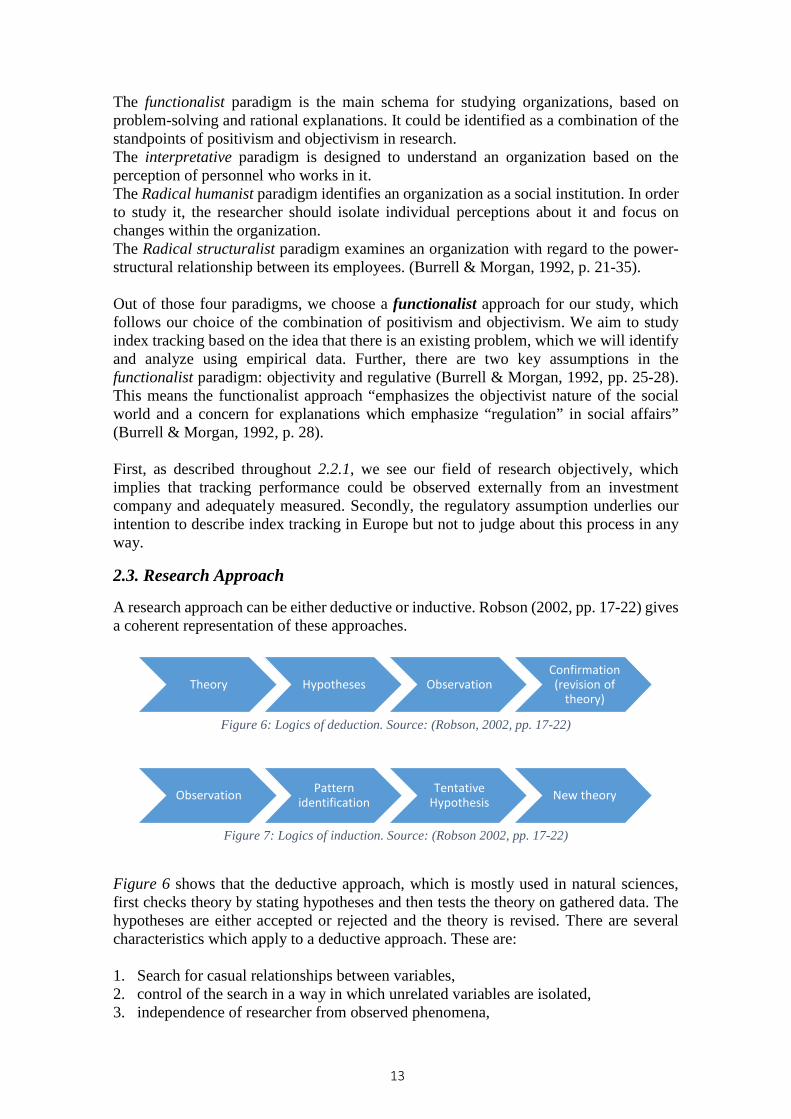
The functionalist paradigm is the main schema for studying organizations, based on problem-solving and rational explanations. It could be identified as a combination of the standpoints of positivism and objectivism in research. The interpretative paradigm is designed to understand an organization based on the perception of personnel who works in it. The Radical humanist paradigm identifies an organization as a social institution. In order to study it, the researcher should isolate individual perceptions about it and focus on changes within the organization. The Radical structuralist paradigm examines an organization with regard to the power-structural relationship between its employees. (Burrell & Morgan, 1992, p. 21-35). Out of those four paradigms, we choose a functionalist approach for our study, which follows our choice of the combination of positivism and objectivism. We aim to study index tracking based on the idea that there is an existing problem, which we will identify and analyze using empirical data. Further, there are two key assumptions in the functionalist paradigm: objectivity and regulative (Burrell & Morgan, 1992, pp. 25-28). This means the functionalist approach “emphasizes the objectivist nature of the social world and a concern for explanations which emphasize “regulation” in social affairs” (Burrell & Morgan, 1992, p. 28). First, as described throughout 2.2.1, we see our field of research objectively, which implies that tracking performance could be observed externally from an investment company and adequately measured. Secondly, the regulatory assumption underlies our intention to describe index tracking in Europe but not to judge about this process in any way.

2.3. Research Approach

A research approach can be either deductive or inductive. Robson (2002, pp. 17-22) gives a coherent representation of these approaches.

Figure 6: Logics of deduction. Source: (Robson, 2002, pp. 17-22)

Figure 7: Logics of induction. Source: (Robson 2002, pp. 17-22)

Figure 6 shows that the deductive approach, which is mostly used in natural sciences, first checks theory by stating hypotheses and then tests the theory on gathered data. The hypotheses are either accepted or rejected and the theory is revised. There are several characteristics which apply to a deductive approach. These are: 1. Search for casual relationships between variables, 2. control of the search in a way in which unrelated variables are isolated, 3. independence of researcher from observed phenomena,

Theory Hypotheses ObservationConfirmation (revision of

theory)

Observation Pattern identification

Tentative Hypothesis New theory

13

4. operationalization, which requires objective measurement of observed changes, 5. generalization as a final goal; in deduction the researcher should revise theory or agree

with existing theory. (Gill & Johnson, 2010, pp. 46-52). An inductive approach, as demonstrated in Figure 7, is the opposite of deduction. It endeavors to develop theory from gathered data. The idea is to establish views on phenomena by gathering data and try to explain observed patterns by creating new theory. Such an approach is usually regarded as highly scientific. It is time-consuming but outcomes are distinct and look deeply into the observed subject in order to find potent explanations (Easterby-Smith et al., 2012, pp. 39-45). Our research is deductive. We state hypotheses based on existing theories and test those hypotheses using empirical data from Datastream obtained for a period of 10 years. By comparing the data of two indices tracking funds we can assess theories found about index fund tracking. By carrying out a statistical analysis using differences in tracking efficiency as a basis, we will be able to analyze and evaluate our hypotheses about index tracking of European indices and draw a conclusion about possible relationships between the two investment instruments. By means of carefully established data selection criteria (as presented in 4.1.4) we seek to keep the results free of uncontrolled influences. We further discuss our results against the background of previous theory and either agree or disagree with existing theory. In the letter case (and if our results are generalizable), we present a revised perspective for European Index trackers. In a nutshell, our study is deductive, has a positivist position and, according to ontological assumptions, takes an objectivistic approach. We see these standpoints as typical for quantitative research; however, a change of any standpoint could be regarded as an opportunity for further studies.

2.4. Research Method

Adams et al. (2007) point out the importance of the difference between research methodology and research method. While methodology is the science and philosophy behind all research, the research method describes the way of conducting and implementing the research (Adams et al., 2007, p. 25). Depending on the research question, the research techniques and procedures have to match the purpose of the study and be aligned with methodological choices in a way that best serves the objective. After having taken our methodological stance, we shall now motivate our choice of research method for this work.

There are two common domains of research method which can be used separately or in a combined approach. One of the methods is the qualitative method of data collection and analysis. It is often used to describe reality as experienced by individuals and is rather used in connection with verbal or written (non-numeric) data than with numerical data (Adams et al., 2007, p. 26). The flexibility during the inquiry of such data leaves room for subjectivism throughout the interpretation but at the same time limits the generalizability of the results from an individual sample to a population. Generating or using numerical data, by contrast, is known as quantitative research. Most statistical analysis is based on quantitative data which can be measured numerically (Adams et. al, 2007, p. 85).

14

Even though by the end of the 20th century research was dominated by quantitative methods, in the recent past, the qualitative method became of increasing importance. This development is, among other aspects, explained by a shift towards a more subjective and culture-bound approach to research in order to conduct more socially and culturally sensitive research. The most recently used and third method is an approach which combines quantitative and qualitative methods by using both quantitative and qualitative data as well as suitable analysis techniques. Tashakkori and Teddlie explain the existence of the mixed method as a result of the possibility that a single research project can contain two paradigms or two worldviews (Tashakkori & Teddlie, 2002, pp. 5-11).

While many researchers nowadays make use of a combination of both methods (mixed method), we see our research purpose best served using a quantitative research method. This serves our needs the best, since we make use of numerical secondary data in the form of historical fund returns and index returns which will be the basis for statistical tests and tracking error estimates. These returns are predetermined by the market and will, due to our strongly objectivistic ontology, be accepted without any subjective interpretation or modification steered by our own conception.

Apart from choosing the quantitative method, we classify our research as a longitudinal study. Longitudinal studies cover long periods of time and follow the sample multiple times. This not only provides us with the desired knowledge about the behavior of two different fund models over the chosen period but also with the ability to answer questions about causes and consequences. This helps us to break down our series into different periods of interest and analyze them separately (cf. Adams et al., 2007, p. 27). In our case the choice of a longitudinal study is implied as we aim for evidence about the tracking capability of Index Funds over time and thus have to consider a longer timeframe instead of a “snapshot” time horizon as described by Saunders et al. (2009, p. 155). The latter method is referred to as cross-sectional study and is used to observe a particular phenomenon at a particular time, i.e. how a trigger event affects one or more objects under investigation.

2.5. Choice of Literature and Critical Assessment

The use of electronic media such as the internet increases the accessibility of data significantly. Search engines and a huge variety of databases open doors too an extensive amount of information, which can have many benefits for researchers in conducting data collection. Besides the obvious advantages this kind of data holds, like every source, electronic media have to be evaluated carefully especially in view of the extensive amount of data and their simple accessibility by everyone. Thus, filtering for relevance and reliability is increasingly important and difficult. Therefore, we have to find ways to structure our inquiry in a way that narrows the bulk of material down to the most useful and reliable selection.

Why Literature Review? Throughout this paper we analyze tracking performance of mutual index funds and ETFs by means of a deductive research approach. In other words, we do not intend to develop new theory but base our hypotheses on previous findings. This approach implies the need of a literature review. A literature study is needed in order to find answers to questions such as what has been done in previous research, what the main theoretical perspectives in the subject area are and what the common methods of investigation are. Reviewing previous literature further gives us information on who are the experts in the field and what are the commonly accepted findings and controversies. (Adams et al., 2007, p. 49)

15

The review of a large amount of articles gives us a clear picture on the current stage of research. It further generates a selection of papers which are closely related to our research question and thus can be used as basis for our hypotheses and as point of connection for our discussion of results.

2.5.1. Choice of Sources

Saunders et al. (2009) categorize literature sources according to the flow of information from the original source (primary literature) to secondary and tertiary sources, where the level of detail increases from the latter to the first stage. As the different stages build on each other, the level of accessibility increases if literature is published at a later point in information flow. (Saunders et al., 2009, p. 64)

It may be unrealistic for us to conduct our study with primary literature only, which in our case is especially limited due to time and cost restrictions. The majority of our chosen literature is therefore of secondary nature which, if carefully selected, does not lead to pivotal quality constraints. Where possible we make use of primary sources such as governmental publications, which nowadays are often made accessible via the Internet.

In order to structure our literature research we focus on articles published in well-established peer reviewed journals (e.g. Journal of Portfolio Management, Journal of Financial Markets etc.) and further track back crucial information by searching for the respective articles included in the reference lists. Our choice is further dominated by more recent articles (mainly 2000-2012) due to the fact that Exchange Traded Funds reached their main adoption in the beginning of the 21st century. Due to low reliability we widely avoid Internet publications and commissioned articles. If we decide to make use of such sources we treat them with the necessary caution with respect to possible bias.

Several electronic libraries mainly made available by the Umeå University Library provide us with access to a broad amount of scientific papers. Besides other sources, the most frequently consulted databases for articles in the course of our research were Business Source Premier, hosted by EBSCO Publishing Inc. (EBSCO, 2013), and LIBRIS, a Swedish national search service providing a joint catalogue of the Swedish academic and research libraries (LIBRIS, 2013). Some of the most frequent keywords for our requests included “Mutual Index Funds”, “Exchange Traded Funds”, “Tracking Error”, “Index Replication” and “European Index Funds”.

To gather information about included funds and indices we retrieved general input from well-known financial market platforms such as Bloomberg, Morningstar, Yahoo Finance and more detailed information from the respective fund company’s website. The daily data for fund returns was solely obtained via Thomson Reuters Datastream, which is also made available to us via the Umeå University Library. Datastream is widely viewed as one of the largest global databases of economic data, covering up to forty years of historical financial information (Umeå Universitetsbibliotek, 2013). A more detailed

Figure 8: Flow of Information. Source: Own design motivated by Saunders et al. (2009, p. 69.)

16

description of the financial data used will follow in the course of this study throughout chapter 4. Quantitative methods in our study are based on statistical analysis. We used t-tests for a mean, paired two samples t-tests, regression analysis, descriptive statistics and analysis of variance methods. The description of methods in detail is provided in chapter 4, but in terms of sources to describe the statistical tools used, we refer mainly to books from our University library. Frequently used books were “The Practice of Statistics for Business and Economic” (Moore at al., 2011) and David Ruppert’s “Statistics and Data Analysis for Financial Engineering” (2011). These books provided us with the main necessary knowledge for statistical analysis.

2.5.2. Data Type

During our study, main results will be based on secondary data; returns and net asset values of index funds and hedge funds obtained from Datastream. The choice regarding secondary data has such advantages as:

• Fewer resources needed. According to Ghauri and Gronhaug (2005, p. 95) it is less expensive to use secondary data than collect data yourself. • Less time needed. Cowton (1998, p. 430) demonstrates that researcher won’t need a lot of time to collect needed secondary data. • Suits longitudinal studies (Dale et al., 1988, pp. 50-60) as such type of data may contain information for a period of years. This feature is of utmost importance to us, as we implement longitudinal comparison of tracking index funds. • Conforms to comparative tasks of researchers (Saunders et al., 2007, p. 259). Secondary data is suitable for comparison in order to assess generality of findings. • Guarantees permanence, unlike other types of data, secondary data is permanent and easy available for others, thus the data is more open to public scrutiny (Denscombe, 1998, p. 180).

There are also disadvantages of secondary data. According to Denscombe (1998, p. 182) and Saunders et al. (2007, p. 260) data may not fit the purpose of the study or regarded with less quality. As our main source is the Thomson Reuters Datastream intellectual network (Datastream) we trust in the quality of our data, which is due to high reliability and validity of data provided by Datastream (Datastream, 2008, pp. 1-2).

2.5.3. Quality Assessment of Sources

Literature review and the selection of secondary literature is a critical part, as we rely on third party information. There are several aspects regarding relevance, quality and accessibility that should be scrutinized.

The freedom of information inherent in electronic media comes with benefits of accessibility and simplified distribution possibilities on the one hand, but with a higher risk of an insufficient level of quality on the other. Therefore, we maintain a number of principles in order to ensure the quality of our study.

First, we make use of our own judgment; once we select an article to review we look at several indicators, i.e. who is responsible for the work, who published the work, when was it published, what is the overall impression of the style and the flow of arguments that lead to the presented evidence and which other works does it refer to (Adams et al.,

17

2007, p. 61). Instead of fundamental works, we rather focus on recent articles than older ones, which might be outdated. Even though this does not always constitutes a sufficient measure of quality, personal judgement gives a first impression of which literature to further focus on and which literature should be treated with caution.

Second, as mentioned before, we search for articles published by well-known scientific journals. As we are facing an enormous number of different journals in the field of business administration and economics, we make use of a journal rating provided by the Australian Business Deans Council (ABDC). The ABDC established a Journal Quality List, which considers the relative standing in other recognized lists (such as the Association of Business Schools), citation metrics, international standing of the editorial board, the quality of the peer-review process and others (ABDC, 2013). The lists contains only recognized journals and ranks them from A* over A, B to the lowest rating C. During our literature review we avoid unlisted journals and prefer highly ranked ones.

2.6. Ethical Considerations

“Ethics pervade the way we live our lives. The dos and don’ts are only part of ethics and moral issues… Research ethics covers the ways in which research is conducted and reported.” (Errikson and Kovalainen, 2008, p. 62) Ethics in research deals with sets of expedient behavior in relation to the subject of study. Cooper and Schindler (2008, p. 34) identify research ethics as standards of behavior in relation to others. In business studies there are two streams with regard to research ethics: deontology and teleology. The former states that no matter what the research results are and how significant a research is, it should be ethical. The latter, in contrast, agrees that research might go unethical ways in order to achieve “higher results”. For our preliminary search we use the Internet. Not long ago Cooper and Schindler (2008, p. 36) highlighted a concept of netiquette. It refers to ethical behavior while using the Internet in relation to interacting with possible participants or privacy limitations. The authors of this thesis take ethical considerations not only for granted but also as a very important and serious element throughout the whole research process. We therefore comply with the deontology concept and believe that research can be done only in an ethical way. In order to reach a high ethical standard we adhere to the ethical guidelines of Umeå School of Business (USBE) in particular, which are made available to students via Cambro (2013), and to ethical codes of society in general. Both authors undertook and passed the obligatory “mini-exam” about academic ethics at Umeå Business School. Our research project does not include any third party participants. Thus, aspects of ethical consideration related to participants such as contacting participants, privacy invasion, consent issues and appropriate information of participants are insignificant to our research. We will discuss and analyze returns of index tracking funds. These were obtained from Datastream, which, as already motivated, has the reputation of a highly reliable data source. Further, all information, which we use are freely available to market participants and thus cannot be harmful if disclosed. The findings from our study embrace different factors which may affect others’ decisions in case they will use our findings (Khang et all. 2012, p. 280). Thus we are concerned to remove any bias or false conclusion from

18

our study and the report about the results, and we endeavor to achieve an objective underpinned by reliable data conclusions. We further indicate and properly reference all stated ideas and intellectual property of third parties and provide the respective bibliographic information to give other researchers the possibility to verify this work.

2.7. Summary of Methodological Choices

During the appraisal of our project’s methodological assumptions, we decided to implement a positivist stance with objectivist concerns by performing quantitative research in a deductive way over a defined time horizon (10 years). A visual summary is provided below in the Figure 9.

Figure 9: Methodological summary. Source: own design.

2.1

• Pre-understanding: high level of awareness• Background of researchers: M. Sc. in Finance• Objective: conduct a genuine research thoretical and practical

contribution

2.2

• Research Philosophy• Ontology: Objectivism• Epistemology: Positivism• Paradigm: Functionalist

2.3• Research Approach: Deductive (Hypotheses testing)

2.4• Research Method: Quantitative study; Longitudinal research

2.5.1

• Choice of Sources• Search Tools: EBSCO, Datastream, Elsevier, Journal of Finance• Relevance, sufficiency, quality oriented

2.5.2(3)

• Data Type: Secondary Data• Quality of Sources: own judgement, peer review, ABDC quality

rankings

2.6• Ethical Considerations: high ethical standards, guidelines of Umeå

Business School regarding ethical conduct in research

19

3. Theoretical Framework Throughout this chapter we give an insight into the characteristics of the two different types of investment companies we aim to compare to one another. Furthermore, we introduce important terms and definitions that we make use of throughout this paper. Among other aspects we discuss the calculation of return differences, tracking error and indices as it was covered in previous literature. We conclude our literature review with a selection of relevant findings published by other researchers that we find to be connected to our research purpose and appropriate bases for our hypotheses.

3.1. Index

3.1.1. Definition and Use of an Index

Financial indices are frequently used to capture information about regional, industrial or sectional markets of economic interest and their development. Thus, the purpose of an index might be for instance to represent a geographical or political region (e.g. Asia, South America, Europe, continental Europe or the EU), a country’s economic development (e.g. France, Germany, Spain), an industry (health care, entertainment, food) or a sector (e.g. emerging markets). Further, indices can be specialized in specific themes or strategies like sustainability, dividends, sports etc. Today, a huge variety of fields in all respects is covered by indices, which enables their inclusion into investment strategies or market research. (cf. inter alia Jordan & Miller, 2009, pp. 152–158).

One of the most followed stock index is the Dow Jones Industrial Average™ (or Dow©), which comprises large and well known U.S. companies (McGlone, 2011) followed by the Standard and Poor’s 500 index containing 500 of the largest companies of the U.S (Standard and Poor’s, 2012). As for Europe (and for the relevance of this thesis), the most common stock market indices are CAC40, FTSE 100, IBEX 35 and the DAX 30, tracking the largest French, UK, Spanish and German stocks respectively. On a European level, common indices are the EURO STOXX 50 (50 stocks from 12 Eurozone countries) and the MSCI Europe (consisting of 16 developed market country indices). (MSCI, 2013; STOXX, 2013).

Indices such as the above listed can project a thorough picture of the underlying markets. Accuracy in reflecting the true values and development is, however, limited due to index staleness. Index staleness occurs when an index includes stocks which are not traded on a daily basis and therefore compromise the indices monitoring accuracy. Therefore, such stocks might not be represented by the index, even if playing an otherwise influential role. By not including every single stock that determines the represented market but rather a portion of it, indices cannot mirror this market 1:1. (Jordan & Miller, 2009, p. 152)

Armstrong names further problems of indices that investors might have to be aware of. Firstly, many indices (e.g. the S&P 500) are weight included securities by market capitalization. With increasing value of a constituent, this stock becomes more influential to the index in the same time and thus makes the index more vulnerable to concentration, i.e. that a few stocks tend to be taken as representative for the underlying market. Secondly, many investors use indices as basis for diversification strategies. Growth in particular sectors is being passed on via a respective emphasis in the index and thus can dilute expected diversification. The same applies for investment style, should one style start to dominate (e.g. growth vs. value stocks). (Armstrong, 2011)

20

3.1.2. Index Calculation

Financial indices may be calculated in different ways. In general, the procedure is called weighting. There are capitalization-weighted, equal-weighted, modified market capitalization weighted, price-weighted and attribute weighted indices. While FTSE, MSCI, S&P and Dow Jones mainly use capitalization weighting for index calculation, the Dow Jones Industrial Average is an example for a price-weighted index (S&P 500, 2012, p. 4). Devisor of an index In order to understand weighting, it is important to introduce the term “index devisor” first. It is used to present index in a suitable way. To get an index price, one should for each stock in the index obtain their market capitalization (price of the stock x No. of shares outstanding) and sum up all the results. For the S&P 500, for example, this would be around $12 trillion nowadays. For convenience, a divisor is used to divide the index price by and thus to get lower numbers to work with. In case of the S&P 500, in the beginning the devisor was determined by market capitalization in the base year 1943. It then was adjusted, if any changes occurred in stocks, which changed the market value of the index but left stock prices unaffected. Thus, in case of stock splits, issues of additional shares, changes in index composition, etc. the divisor is tuned to keep the index on the same level. The general formula for the divisor is:

𝐷𝐷 = 𝐷𝐷𝑡𝑡−1 ×𝑀𝑀𝑀𝑀𝑡𝑡𝑀𝑀𝑀𝑀𝑡𝑡−1

Equation 1: Index Divisor In Equation 1, D is a new devisor and MV is a market value of an index. The devisor is always adjusted to cancel out any changes of index price at t-1, if they are not related to constituent stock prices. If we suppose that S&P 500 closes at 1250 and one company performs a share repurchase, in order for S&P 500 to open at 1250 next day, the shares repurchase is canceled out via devisor adjustment. (S&P 500, 2012, p. 5).

Market weighted index For Market weighting (also capitalization weighted or value weighted) the index is calculated as a sum of the market capitalization of all shares belonging to the particular index. The formula is

𝐼𝐼𝐼𝐼𝐼𝐼𝐼𝐼𝐼𝐼 𝑃𝑃𝑃𝑃𝑃𝑃𝑃𝑃𝐼𝐼 =∑ 𝑃𝑃𝑖𝑖 × 𝑄𝑄𝑖𝑖𝑖𝑖

𝐼𝐼𝑃𝑃𝑑𝑑𝑃𝑃𝑑𝑑𝑑𝑑𝑃𝑃

Equation 2: General MW index calculation

with P as the stock price and Q as the number of share outstanding. Market weighting (MW) is commonly used and most of the S&P indices, Dow Jones indices as well as FTSE, MSCI, AEX and others EU indices are capitalization weighted (S&P 500, 2012, p. 6). Nowadays, most indices (e.g. S&P 500, CAC 40, FSTE, AEX, MSCI etc.) are modified, e.g. by using free-float adjustment or other methods which we will briefly discuss next.

Market weighted index: Capped factor A capped weighted index constrains constituents to a specified weight and the excess weight is spread among the remaining index constituents. Thus, it limits the weight on a

21

stock, which has “too high” market capitalization. As stock prices change, the weights will shift and the adapted weights will change. Similar to an equal-weighted index and a modified market cap index, a capped market weighted index must be rebalanced from time to time to re-establish the correct weighting. The procedure is similar to market cap weighted indices. The main difference between the methods concerns adjustments of corporate actions between rebalancing periods. For modified market cap weighted indices most corporate actions which affect the market capitalization of a given stock are counterbalanced by a corresponding change in the adjustment factor assigned to the stock in that index, thus resulting in no weight change to the stock and no index divisor change. For capped indices, by contrast, no adjustment factor change is made due to corporate actions between rebalancing, and thus the weights of stocks in the index as well as the index divisor will change due to corporate actions. (S&P 500, 2012, p. 19).

Market weighted index: Floating factor Using a market weighted method with a floating factor means that the number of shares outstanding is reduced, in order to represent shares which are available to investors by excluding closely held shares (e.g. some stocks are closely held by the government, long term investors, or the company itself). Thus, such adjustment allows only freely traded shares to be considered for index calculation. The adjustment requires having Investible Weight Factor (IWF), a percentage of shares outstanding and freely available for trading. Thus, in case of free float adjustment, the number of shares is adjusted by the formula 𝑄𝑄𝑖𝑖 = 𝐼𝐼𝐼𝐼𝐼𝐼𝑖𝑖 × 𝑇𝑇𝑑𝑑𝑇𝑇𝑇𝑇𝑇𝑇 𝑆𝑆ℎ𝑇𝑇𝑃𝑃𝐼𝐼𝑑𝑑𝑖𝑖. Afterwards Q is used in Equation 2 above for index price calculation (S&P 500, 2012, p. 7). Market weighted index: other adjustments In addition to already mentioned modifications, it is possible that an index could be specially modified. A modified market cap weighted index has a “user-defined” weight in the index. It is used to constrain constituents to specific maximum weights. Modified market cap weighted index also must be rebalanced over time to have a “proper” weighting (S&P 500, 2012, p. 15). Market weighted index: AEX example The AEX index (weighted as free float adjusted market capitalization index) is calculated as:

𝐼𝐼𝑡𝑡 =∑ 𝑄𝑄𝑖𝑖𝐼𝐼𝑖𝑖𝑓𝑓𝑖𝑖𝐶𝐶𝑖𝑖𝑋𝑋𝑖𝑖𝑁𝑁𝑖𝑖=1

𝐷𝐷𝑡𝑡

Equation 3: General MW index calculation

Where Q is the number of shares of equity in the day t; F is a free float factor of equity i; f is the capping factor (currently 15% for AEX index) which is used to limit the weights of the stock if they exceed a certain percentage of equity i; C is the price of equity I on day t; X is the current exchange rate on t and D is the divisor (as described above in Equation 1) on day t (on 10 May 2013 D was 748415614,163642 for AEX) (AEX, 2013).

Market weighted index: criticism Recently, market weighted indices calculation methods were put to scrutiny and criticism. Recent studies argued that MW is no optimal method to create an index portfolio as it provides inefficient risk-return tradeoff (inter alia Amenc et al., 2011; Arnott et al., 2005). Thus, using market capitalization will not provide fair value as index constituents quoted

22

prices are biased with preconceptions of current traders (e.g. overweighed, overpriced, etc.). Therefore, Arnott et al. proposed and patented index weighting using fundamental values of a company. They argue that market capitalization leads investors to buy as prices rise and sell as prices fall, which is in contrast to the “buy low, sell high” strategy. (Arnott et al., 2005, p. 84) In addition, one should not forget that, although an index represents the market state, it also embodies capital flow and bargaining power of participants. Thus, an index price might entail share float, share price and constituent companies influencing the market in their own way (Ghorawat, 2013).

Effectively, market indices are a compound factor of three variable components: 1) the quantity of Share (whether Free Float or Total issued), 2) the prices of the Equity Shares and 3) the constituent companies of the Market Index, each influencing the determination of the state of the capital market (and hence the marked index) in its own manner (Ghorawat, 2013).

Equal-weighted index In this type of index, every stock has the same weight and a portfolio that tracks the index will invest an equal dollar amount in each security. As stock prices move, the weights will shift and exact equality will be lost. Thus, such index would need to be adjusted accordingly (S&P 500, 2012, p. 12). Fundamentally weighted index Using fundamental weighting requires measuring index based on stock fundamental values, which are represented by book value, P/E, P/B, dividends, revenue and gross sales. Fundamental indexation was first introduced by Arnott et al. (2005) and is based on the idea that prices are no good representatives of the current value of a stock. Thus, market capitalization should be avoided due to bias in prices. The article using back testing gives significant returns in comparison with index, however as main opponents argue, such returns were achieved without incurrence of transaction costs, which would substantially eat all the profits due to a need of frequent rebalancing (Arnott et al., 2005). Index weighting comparison Figure 10 below provides insights into three approaches. It is observed that MW indices would be more tax efficient and would have lower expenses. In contrast, Fundamentally Weighted indices would have higher turnover and show specific valuation, which is not biased by market conditions but rather grounded on companies’ balance sheets.

23

Figure 10: Index weighting comparison. Source: Shaw (2008)

Price-weighted Index Price-weighted calculation of an index uses prices of stocks as weights for index price calculation. This type of weighting was criticized a lot as it does not show the real situation on the market. This weighting gives high weights to stocks with high values, and many small value stocks are not considered. A $100 stock, for instance, would have more weight than a $5 stock, disregarding their respective capitalization and company characteristics. In addition, stock prices usually do not show fair value and could be influenced by stock splits or other corporate actions. Finally, such indices should be constantly rebalanced to reveal changes in stock prices. The most popular price-weighted indices are the DJIA and Nikkei 225 (S&P 500, 2012, p. 23). Other weighting techniques Recently, some new methods of weighting have appeared. We shall list them and only give a brief description; such types of index weighting are rather exotic and not used by the major indices such as those we have included in this paper. Since 2005, S&P 500 Pure Style Indices are attribute weighted, where weights depend on the measures of stock growth or value attributes (S&P 500, 2012, p. 23). Indices can also be based on low-volatility, where one would limits the volatility of the tracking portfolio to smooth price changes relatively to a normal index in order to control the level of volatility. Income-focused indices pick stocks with the highest dividends. Dynamic indices try to focus on “attractive” stocks with high momentum. Factor indices track stocks with high beta or momentum. Leveraged indices are designed to generate a multiple of the return, either positive or negative, which is defined by the index. Further, inverse indices provide investors with opposite performance of the chosen index. Next, there are many fund strategies indices, which are created by funds. Their strategy is usually to beat the given benchmark. Dividend indices would track dividend payments from the constituents of a chosen index. The above is not a complete list of index types. There are other types of indices which make the investing universe broader and provide different solutions for the needs of investors (e.g. risk control indices, currency hedging indices or excess return indices) (S&P 500, 2012, pp. 27-50).

24

3.1.3. Index Specifics: The Example of the S&P 500

Different indices possess characteristics which should be considered when one chooses a particular index as a benchmark. S&P is one of the main indices in the U.S. Thus, many portfolios use it as a benchmark, and any change in it also effects prices in stocks, since many managers will trade ahead on those predicted changes to take advantage of the expected price of an index. Before October 1989, changes in the composition of the index were announced at the end of the day when trading was closed. Thus, the changes effected opening prices of an added stock on the next day and vice versa for a deleted stock. After 1989, S&P 500 changed their policy and announced additions or deletions as early as possible to give more opportunities to people to profit from them (Chiang, 1989, pp. 310-312). Furthermore, in terms of dividends in the mid-80s, the index reinvested dividends every quarter, and it was easier to track an index by funds during up markets as they could reinvest dividends earlier. Nowadays, the index is calculated assuming that dividends are reinvested immediately if the stock goes ex-dividend. This has important implications for index funds, as it makes tracking harder due to the deferral between actual dividend distribution and the moment when index managers receive them. (Chiang, 1989, p.311).

3.2. Return, Risk and Error

3.2.1. Return Difference

Return difference is a measure of how the return deviates from its benchmark over a given period. Return difference is calculated as shown in Equation 4 below, where 𝑅𝑅𝑖𝑖 is the return of an index fund and 𝑅𝑅𝑏𝑏 is the return of the tracked benchmark index.

𝑅𝑅𝐼𝐼𝑇𝑇𝑅𝑅𝑃𝑃𝐼𝐼 𝐼𝐼𝑃𝑃𝑓𝑓𝑓𝑓𝐼𝐼𝑃𝑃𝐼𝐼𝐼𝐼𝑃𝑃𝐼𝐼(𝑅𝑅𝑑𝑑) = 𝑅𝑅𝑖𝑖 − 𝑅𝑅𝑏𝑏

Equation 4: Return Difference

When tracking index, a certain return difference is expected. This is due to the fact that the tracking index is a “paper only” index and it does not experience any market fees or frictions. It is created solely for benchmark purposes and not a subject to tradable securities regulations, such as broker fees and taxes (Frino & Gallagher, 2001, pp. 4-5). This implies that returns of an index fund should always be smaller than returns of an index. When weights in the index change due to changes in volume or prices of the securities, for instance, the index adjusts the new portfolio weights automatically and calculates the value. As tracking proceeds, a portfolio manager needs to adjust his weights by performing real transactions on the market, which is subject to broker fees and taxation. Therefore, there will always be a return difference between an index tracking fund and its benchmarked index. The difference in a perfect market condition is expected to equal the amount of transaction costs (Frino & Gallagher, 2001, p. 5). According to Chiang (1998) the main drivers of return differences are transaction costs, fund cash flows, the treatment of dividends by the index, the volatility of the benchmark and index composition changes. In addition, one could say that there will always be a tradeoff between minimization of return differences and cost minimization. Portfolio managers will decide when they should rebalance the weights and become more efficient in tracking an index on the one hand. On the other hand, they prefer to keep weights

25

unchanged in order to avoid transaction fees and stay cost efficient. Therefore, a manager’s decision is always a compromise aimed at reducing the return difference (Frino & Gallagher, 2001).

3.2.2. Tracking Risk

Tracking error as a measure for tracking risk was first defined by Tobe in 1999 (Tobe, 1999) as a percentage difference. Nowadays it is calculated as a standard deviation of return differences. It measures deviations in index tracking.

TE = �∑(𝑅𝑅𝑑𝑑−𝑅𝑅𝑑𝑑���� )2

𝑛𝑛−1

Equation 5: TE as defined by Tobe (1999)

In Equation 5, 𝑅𝑅𝑑𝑑���� is return differences mean and 𝐼𝐼 is a number of observations. In denominator 𝐼𝐼 − 1 is used, and not 𝐼𝐼, because our estimation of tracking error is based on a sample. Thus, according to Bessels’s correction (cf. entry for ‘variance (data)’ in Upton & Cook, 2008), we use an unbiased estimator of the variance of population in order to calculare Tracking Error.

One could see that the TE is simply a standard deviation, which can be defined as

𝑇𝑇𝑇𝑇 = �𝑑𝑑𝑇𝑇𝑃𝑃(𝑅𝑅𝑃𝑃 − 𝑅𝑅𝑏𝑏)

Equation 6: Tracking Error Estimate

Equation 6 makes sense, as we use TE to estimate a variance of return differences. If TE is vast, we can conclude that tracking is performed poorly and that there are high dispersions between index funds and benchmark index return (CFA, 2012, p. 473). TE may be used as a probability measure. For example if TE is 3 percent annually (which means that we use annual return differences), under the assumptions of cumulative standard normal distribution, the probability that index fund returns will vary from +3 to -3 percent is 68%. This means in turn that the fund may outperform or underperform an index with a probability of 16 percent. Normally, TE had not exceeded 2 percent until 1999 (Lawtone-Browne, 2001, p. 224,226). TE is often used as a key ratio for fund selection process; it is also a goal estimator for a fund and a measure of performance of an index fund manager (Chiang 1998, p. 308). The causes of tracking error are tightly connected with return differences and represented in the form of costs, replication methods, turnover, management experience and enhancements (Chiang 1998, p. 308). Several authors claim that using standard deviation to measure risk of deviations of a fund from a benchmark is inappropriate due to return distribution characteristics; however, if we take samples from the market as a whole and use a long time horizon, the standard deviation should be a reasonable estimator of risk (Louargant et al., 2006, p. 193).

26

In academic literature, TE minimization is a problematic process. Roll (1992) tried to solve the asset allocation problem, and, under the constraints of minimal TE, was not able to obtainea mean-variance efficient portfolio. In addition, Ammann and Zimmermann (2001) showed that while return correlations within a fund falls, TE raises. Furthermore, according to research by Lawtone-Browne (2001, p. 224) tracking error could be easily underestimated due to the fact of volatility clustering, which violates stationarity of volatility. The above presented Equations 5 and 6 show the most common notation of calculating Tracking Error. Apart from this definition, for our analysis we will make use of two additional estimates which were used by Frino and Gallagher (2001) and will be introduced in chapter 4 of this work.

3.3. Funds

3.3.1. UITs, Open-end and Closed-end Funds

Investment companies provide services for investors who are not professionals in finance. Usually they are separated in open-end funds (mutual funds), closed-end funds (CEFs), or unit investment trusts (UITs). Open-end investment companies or mutual funds In this fund type investors purchase or redeem shares of the fund directly from the company or by contacting a broker. Assets of a fund are reduced when shares are repurchased and vice versa. If an investor intends to buy shares from a fund, according to the security regulations, a prospectus must be disclosed to the potential buyer which has to inform about management fees, other expenses, risks and minimum investments (Anderson et al., 2010, p. 4). Mutual funds which apply a more passive strategy in replicating an index are called mutual index funds (SEC, 2007). This type of fund is being referred to in our study, since we intend to research their tracking performance in comparison to ETFs. Closed-End Investment Companies In a closed-end Investment Company, shares are distributed at an initial public offering (IPO) which is preceded by the issuance of a fund prospectus. After the IPO, money obtained by the fund is invested according to the policy statement in the prospectus. The difference to mutual funds is that the closed-end fund issues shares only once and investors cannot liquidate shares. Instead, they can exchange shares on the secondary market or over the counter (OTC). It should be noted that there are no legal requirements stipulating that the price of the shares should represent the fund’s current assets. Thus the price is determined by supply and demand on the market. Net assets (Assets – Liabilities) divided by the number of shares outstanding gives net asset value (NAV); it is used as a measure of the relationship between stock price and a fund’s assets value.

𝐷𝐷 = 𝑁𝑁𝑁𝑁𝑁𝑁−𝑀𝑀𝑁𝑁𝑁𝑁𝑁𝑁𝑁𝑁

Equation 7: Premium or Discount of Funds

27

In Equation 7, MV is a market value of a share, D is the percentage difference between NAV and MV. If NAV is bigger than MV, it is called a discount. If it is smaller, D is called a premium. Discounts usually prevail on the market (Anderson et al., 2010, p. 4). Unit Investment Trusts Unit Investment Trusts (UITs) offer unmanaged portfolios. For a specific period of time UITs create a well-diversified portfolio, which is fixed over the whole period. Thus, UITs cannot be sold or bought after initiation. Initial sale is usually performed by a broker. The main goal of buying a UIT is to obtain a diversified portfolio for a fixed period for a capital appreciation (stock trust) or a fixed return (bond trust) (Anderson et al., 2010, p. 5). Excursus: Hedge Funds Famed hedge fund manager Mario Gabelli wrote in 2002: "Today, if asked to define a hedge fund, I suspect most folks would characterize it as a highly speculative vehicle for unwitting fat cats and careless financial institutions to lose their shirts" (Gabelli, 2002, p.1). Such statements are remarkable since hedge funds are often referred to as highly profitable investment companies, which use advanced strategies to diversify risk. Negative opinions emerged mainly due to large failures of hedge funds in the 1990s and 2000s. Hedge funds are a limited partnerships, which accept an investor’s money and invests it in a pool of securities by using different enhanced strategies to obtain absolute returns. Such strategies employ arbitrage strategies, event driven strategies, short selling, use of derivatives, and leverage. Thus, hedge funds are popular in bear markets (Bollen & Pool, 2012). One can see that hedge funds are similar to a mutual fund, however, they differ significantly in terms of return goals. To give an example, if the market is down 10% and a mutual fund only 7% it would be a success for a mutual fund. A hedge fund’s target absolute returns, by contrast, are not correlated with the market, and should always to be substantial (around 6 - 9% annualized return). In theory, this had to be achieved by using more sophisticated strategies in comparison to mutual funds. Moreover, hedge funds are not obliged to be registered under the SEC, as only financially sophisticated investors are accepted to invest. To sum up, hedge funds should reduce risk as it is professionally managed by using enhanced strategies. In reality however, hedge funds tend to strive towards higher returns which eliminates safety and leads to high risks and in many cases to bankruptcy (Anderson et al., 2010, p. 6).

3.3.2. Exchange Traded Funds

Exchange Traded Funds are a younger version and a special case of traditional index funds. Both fund types aim to provide investors with access to the return of a certain benchmark. Yet, their characteristics differ with respect to tradability, index replication and creation and redemption process.

Even though the SEC legally classifies ETFs as open-end companies or Unit Investment Trusts (SEC, 2010a), Deville calls ETFs “hybrid instruments”, which combine the advantage of open-end unit trusts and closed-end funds. This combination is explained on the one hand by the ETFs tradability, which is comparable to closed-end funds, and by the ETFs creation and redemption process on the other hand, which takes the form of open-end funds (Deville, 2008, p. 9). In a nutshell, ETFs can be traded on a continuous

28

basis throughout the trading day while designated sponsors (ETF broker) have the possibility to create or redeem ETF units according to the current demand.

Tradability The origin of Exchange Traded Funds and their unique trading characteristics lies in the first Exchange Traded Index Fund to be launched. Released by Standard & Poor’s (S&P), the fund was called Standard & Poors’s Depository Receipts (SPDR), also called “Spiders”, and followed the objective of providing the investment results of the S&P 500 in price and yield performance. Being traded on the American Stock Exchange (like an ordinary stock), one Spider has a price equal to approximately one tenth of the S&P Index. One of the features that distinguish ETFs from Mutual Index Funds and drives sufficient liquidity is their creation and deletion throughout an in kind transaction. (Elton et al., 2002, pp. 454,466)

Creation and Redemption Creation and Redemption is the process of how rising demand for an ETF is served and vice versa. The ability to create and redeem ETF units on a continuous basis (while the markets are open) is unique for ETF companies and essential for their trading characteristics and therefore important to understand forresearchers investigating this fund type.

Even though ETFs are often linked to closed-end funds in that ETF shares can be purchased and sold on exchange markets, the ability to create or redeem ETFs in-kind distinguishes them from closed-end funds (Meziani, 2006, p. 41). In-kind creation means investors can turn in the share the ETF uses to replicate the index plus an additional cash amount in order to receive an ETF Creation Unit (CU). Likewise, Creation Units can be turned in and the stock basket used for replication is received, i.e. an ETF unit is liquidated (Elton et al., 2002, p. 466). This ongoing process is one of the reasons why ETFs tend to trade within a tight band around their Net Asset Value, as any price difference between ETF and stock basis creates arbitrage opportunity that will be used by market makers (Abner, 2010, p. 179; Ferri, 2009, p. 36).

Figure 11: ETF Trading Mechanism. Source: Own design, motivated by Deutsche Bank Research

(2008, p. 8).

29

Figure 11 shows the trading mechanism, including the creation and redemption process of Exchange Traded Funds. It is important to notice, that private investors only have access to ETF shares via the stock exchange and thus cannot request creation units directly from the company. This right is exclusively reserved for authorized participants (APs), who use the premium or discount spread between ETF and NAV to realize arbitrage (Ferri, 2009, p. 36). Once an AP delivered the underlying stock basket to the fund company she receives ETF Creation Units (CUs) in return, which are large blocks of ETF shares, usually numbering up to 50.000 shares. The size, however, can vary according to the respective ETF. She then may sell the ETF shares from the creation unit at the secondary market, i.e. at the stock exchange, and thus provide individual investors with sufficient ETF liquidity (Ferri, 2009, p. 34).

Mutual Index Funds, by contrast, forgo this “in-kind” creation and redemption. Here, investors deliver cash in order to buy fund shares or receive cash in order to redeem them. This leads to additional fund flows, triggering additional transaction costs since the fund management has to invest into the benchmarks constituents itself. Furthermore, Mutual Index Funds have to hold a certain percentage of assets uninvested to meet redemption needs. Due to the dependency on the liquidity of an index constituent stock, Kostovetsky identifies this movement of cash in and out of index funds as a secondary cause of tracking error (2003, p. 82).

3.4. Fund Management

3.4.1. Active and Passive Management

In general, fund management strategies can be labeled as active and passive. Passive strategies are popular nowadays due to intuitive simplicity and overall higher stable returns in comparison to active strategies. Passive investment refers to stock or bond portfolio managing using simple buy and hold or index replicating strategies. One of the examples of passive strategy is index fund management. For example if the Nordea stock constitutes 4% of an index, a fund will allocate 4% of its funds to that stock. According to recent performance measurement, passive strategies outperformed more than 75% of active managers during the past 5 years. During the past 20 years, passive management outperformed more than 80% of active management. (Elton et al., 2010, p. 696) Usually, it is assumed that index funds would underperform an index due to additional costs. However, some studies suggest that it could be the opposite way. This is due to the fact that large indices often miss small stock dividends. In addition, index funds could sell owned stocks to willing investors sometimes above market price, usually if investors wish to shorten a stock, which is, however, not available freely on the market. Given these two assumptions, index fund might outperform an index over long time. It is also clear that no index fund exactly matches an index due to different facts already mentioned above (paper index vs. stock portfolio). This means that in growth markets, the performance of funds tend to be inferior to their performance in down markets. (Elton et al., 2011, p. 697) It is important to mention that although passive management commonly refers to managers, who try to use a buy and hold strategy to replicate an index, this is not always the complete truth. Passive strategy may also involve analysis by using past data. It could, for example, be a passive strategy to buy stocks with low P / B ratios. However, when it

30

comes to forecasting, it is assumed that this is, in fact, an active strategy (Elton et al., 2011, p. 697). Contradicting to passive strategies comes active management. During an active strategy, one should determine a benchmark. It would be used as a measure of performance. Thus management will focus on implementing different strategies to outperform a pre-chosen benchmark, which is usually an index. There is a vast variety of strategies a manger could use; however, there are three most used strategies, which are worth to have a closer look at. These are known as market timing, sector selection and security selection. Market timers focus on changing a Beta of their portfolio according to market forecasts, thus obtaining the desired sensitivity towards the market. Security selectors look for specific characteristics of a stock based on its analysis, and as a result, make a bet against a market by increasing weights of a stock in a portfolio (positive bet) of an undervalued stock and decrease the weights of overvalued stocks. Sector selectors are quite similar to security selectors, but they focus on specific sectors. Possible characteristics of a sector could be industrial classification (energy, banking, utilities, etc.), product classification (e.g. healthcare, services, consumer product, etc.), stock characteristics (e.g. growth stocks, stable stocks, etc.) and sensitivity of a group of stock to specific phenomena on the market (e.g. exchange rates or yield curve). It is common that managers usually specialize in a particular industry due to continuous increase of the specifics of each industry. (Elton et al., 2011, p. 699) It is difficult to determine whether the active or passive strategy is superior, although many recent studies based on the net returns point out that passive strategies perform better. In general, active management has to overcome several categories of costs in order to deliver substantial returns. These categories are:

• cost of forecasting (managers with good forecasting ability usually demand high fees);

• cost of diversifiable risk, as portfolios have more diversifiable risk in comparison

to an index, where the risk is close to zero. Investors usually demand compensation for excess risk;

• higher transaction costs, as active investing usually requires higher turnover in contrast to low turnover in buy and hold strategies;

• cost of taxes due to early gain realization. Actively managed funds have a high turnover and, according to the tax law, should thus recognize tax on the gains if the fund sells stock. Although passively managed funds are also concerned with taxes (e.g. if an investor sells his part, a fund should also recognize taxes on gains or losses), they do not have a high turnover and thus recognize taxes not so often. (Elton et al., 2011, p. 701)

3.4.2. Passive Index Tracking

For our empirical study we focus solely on passively managed index tracker funds. After having distinguished active management from passive management, we now discuss the different forms of passively managed fund companies in more detail. Our main focus

31

regarding this matter lies on open-end index funds and Exchange Traded Funds, which we aim to compare in the course of this paper.

3.4.3. Index Tracking Strategy

As we have seen, due to structural differences between the theoretical construct ‘Index’ and the physical construct ‘Fund’, a certain tracking error in index fund performance is indeed inevitable. Therefore, after having agreed on a fund strategy, emitters have to decide on the further motivations and characteristics of the new fund. It needs to be decided whether the fund portfolio will be actively managed with the attempt to outperform the index performance, or if a passive strategy is aimed at, which gives the fund a pure tracking characteristic within a certain accuracy limit (Wagner, 2002). Since our sole focus lies on passively managed funds, we have a closer look on the replication methods fund managers can make use of in order to reduce the trade-off problematic between replication cost and replication quality.

The first and most intuitive method in building a portfolio that replicates a benchmark’s performance is to invest in all the benchmark’s constituents using exactly the same proportions (Frino & Gallagher, 2001b, p. 3). This straightforward method where managers rebuild a smaller version of the benchmark is called full replication approach. Yet, in practice, a full replication of the index can be unpractical especially when the target index consists of a large number of constituents, which leads to undesirable transaction costs once the index is re-adjusted (i.e. constituents are added, deleted or weights are changed) (Di Tollo & Maringer, 2009, p. 130). A full replicating Index Fund has then to proportionally buy or sell the effected stock to its market value (Blume & Edelen, 2002, p. 12). Tollo and Maringer therefore describe the optimization problem of index tracking as “to find asset weights so that the portfolio’s behavior differs from the benchmark’s as little as possible“ (Di Tollo & Maringer, 2009, p. 130).

3.4.3.1. Physical Replication

Investing directly into the constituent of an index in order to replicate its performance as it is done with full replication, may be called a physical replication approach, as fund management accesses stocks which are an actual part of the index. As was discussed before, full replication is often a non-optimal solution due to the incurred costs. Therefore, solutions have to be found in order to replicate the index performance without fully replicating it.

Another yet physical approach is partial replication (or representative sampling). Here the fund management makes use of a representative sample of constituents, where the chosen stocks in the fund portfolio reflect the same weights with which they are listed in the respective index (Hehn, 2005, p. 9). If a fund portfolio is constructed under transaction costs and liquidity constraints (cf. Bamberg & Wagner, 2000, p. 526), the approach of approximate index replication is especially useful if an index holds a large amount of constituents, including numerous very small (less influential) and few large positions which dominate the direction of performance. To illustrate this, we might takes as an example an index fund tracking the MSCI World Index in 2008. By then, the MSCI World listed 1944 companies. While the smallest constituent made 0,0008% of the index, the biggest made up for 1,8%. Regarding iShares, MSCI World (IQQW) shows that the ETF in 2008 counted 932 companies (cf. Ehmann, 2008). The challenge with physical replication of complex indices is therefore to find the right distribution between the risk of occurring costs and the maximum tolerated tracking error.

32

Sampling can also be achieved by making use of mathematical algorithms to construct a portfolio of a determined number of stocks, which best track the index. Another approach is based on investing using characteristics weights of an index. The usual characteristics are industry, capitalization and sector. If the index consists of stocks from different industries (e.g. consumer products, financials, healthcare, etc.), for example, one would invest in a smaller set of stocks, which matches the index to the amount specified by the characteristics (e.g. same percentage in industrial, financial and healthcare stocks). (Elton et al., 2010, p. 697)

Tracking error vs. Total Return Choosing between full replication and sampling can be a tough task for a fund company. When reflecting on fund replication of the S&P 500 index,1 Blume and Edelen (2002, pp. 8–9) point out the sensitivity of the trade-off when a single index constituent is deleted from the fund portfolio. Hence, following their example, if in the year 2000 a stock was removed from the fund portfolio which represented only 0,07% of the S&P 500 Net Asset Value, the subsequent standard deviation of the Tracking Error would be 2,6 basis points, while the standard deviation of the portfolio return maintains the same as prior to the change. Even though the standard deviation of return remains unchanged where Tracking Error is used by investors to measure the fund management’s tracking ability, an increase in Tracking Error standard deviation can have negative implications for delegated investment objectives (cf. Blume & Edelen, 2002, p. 2).

3.4.3.2. Synthetic Replication

Apart from physical replication, a newer trend in the ETF industry is the more complex synthetic replication. Despite its higher complexity, 64% of the ETFs launched from the year of 2009 decided to adopt a synthetic replication approach. This replication method is based on an exchange between the ETF and a counterparty, and is therefore also called swap-based replication. To set up a synthetic replication, an ETF invests in a stock basket which might, regarding investment strategy and composition, completely differ from the benchmark index. The swap contract then allows for a total return swap between both parties, where the swap partner receives the return of the ETF-emitters stock basket, and in return guarantees to deliver the benchmark indices’ return (Ehmann, 2008; Abner 2010).

As the swap partner has to settle possible underperformances of the ETFs hedge basket, the architecture of a swap-based Exchange Traded Fund transfers the performance risk from the fund emitter to its swap partner (Heidorn, et al., 2010, p. 7). In practice, the swap partner is often the fund’s holding company (Meinhardt, Müller, & Schöne, 2012, p. 1).2

1 The S&P 500 index consists of the 500 leading U.S. large cap equities (Spindices, 2013). 2 cf. inter alia db x-tracker ↔ Deutsche Bank; ComStage ↔ Commerzbank and Lyxor ↔ Société Général.

33

Time ETF Value of Swap Swap-Contractant (Stock

Basket) (Index – Stock Basket) (Index)

Day 0 100 0 (0,00%) 100 Day 1 100 4 (3,84%) 104 Day 2 102 5 (4,67%) 107 Day 3 100 9 (8,25%) 109 Day 4 109 0 (0,00%) 109 Day 5 108 -4 (-3,70%) 104 Day 6 109 -8 (-7,92 %) 101

Table 1: Value Simulation of a Swap. Source: Own design, motivated by Deutsche Bank (2008, p. 8)

This constellation implies a contractant risk in the case of insolvency of the counterparty. According to the European fund guidelines UCITS (Undertakings for Collective Investments in Transferable Securities), this risk must not achieve more than 10% of the fund’s Net Asset Value, which is achieved by the ETFs obligation to hold at least 90% of its NAV (Heidorn et al., 2010, p. 8). In practice, many ETFs overly secure their portfolio in order to eliminate the contractant risk.3

Table 1 shows a fictive example of a swap-based index replication with the ETF-company on the one side and the swap contractant on the other (usually the ETFs holding company). At day 0 the swap agreement between both parties is made and the initial stock basket is build up in such a way that its NAV exactly corresponds to the present NAV on the benchmark index. In our scenario, the value of the index climbs from 100 to 104 at the first day after the agreement. This leads to a deficit of the ETF stock basket, which has to be aligned by transferring funds from the swap partner to the ETF. The value of the swap from the ETFs’ perspective increases to 4 and a contractant risk of 3,84% (4/104). On day 3 the stock basket’s NAV reverses to its initial value, while the index NAV continues to increase to 109, which leads to a swap value of 9 and to a contractant risk of 8,25% (9/109). The risk ranging closely to the allowed maximumis a strong sign for the fund management to react by resetting the swap; therefore, the swap partner transfers the swap value of 9 to the ETF, which then uses the funds to reinvest in the stock basket so that the baskets and the index NAVs are aligned again. Day 5 shows the reverse development, i.e. the index NAV decreases against the stock basket. The incurred payment from ETF to the swap partner implies a negative swap value and is seen as over-collateralization of the swap. To avoid growing over-collateralization, an equivalent amount of the stock basket can be liquidated and paid to the swap partner.

While investigating differences in tracking error of German ETFs that use full replication in contrast to those using synthetic replication, Meinhardt et al. found that, even though German ETFs suffer from high tracking errors, the choice of either of the replication methods cannot be explained by the tracking error (Meinhardt et al., 2012, p. 13). According to their research, the decision can rather be explained due to the liquidity or illiquidity of the benchmark index. Thus, it can be more convenient to use synthetic replication in order to replicate an index with illiquid constituents.

3 cf. inter alia db X-trackers CAC 40® UCITS ETF with a net swap exposure of currently 2,45% (db X-trackers, 2013).

34

3.4.4. Fund Related Costs

Investment companies commonly try to attract new investors by advertising their passive index trackers with low management fees as compared to fees of enhanced funds. In fact, Hübscher states that costs are the most important reason why managers of active funds experience difficulties beating the index (2005, p. 77). Khorana et al. found that Index Funds consistently charge 36 basis points lower management fees than actively managed funds (2009, p. 1295)

Hübscher further names the factors which lead to this difference in costs for actively managed funds-.

Management Fees – Significant higher Management Fees due to the need for analysts, researchers etc. for maintaining an active portfolio

Trading Costs – While passive portfolios cause a turnover of usually around 10% per year, active funds have a turnover between 75-100% p.a. This leads to higher trading costs due to Brokerage Fees, Taxes, Spread and Market Impact in relation to passive portfolios. (Hübscher, 2005, p. 78)

Total Expense Ratio Beside management fees, which include charges for management services, a more common and conservative measure is the fund’s Total Expense Ratio (TER). TER covers all annual operating costs and is defined by Morningstar as follows:

"The expense ratio typically includes the following types of fees: accounting, administrator, advisor, auditor, board of directors, custodial, distribution (12b-1), legal, organizational, professional, registration, shareholder reporting, sub-advisor, and transfer agency. The expense ratio does not reflect the fund's brokerage costs or any investor sales charges." (Morningstar, 2013).

As apparent in the definition, the expense ratio misses brokerage costs. Since TER frequently serves as a target ratio for fund managers, Herring and Hunke explain this lack of inclusion through the need of Managers to react to recent market developments even if this means to exceed the target expense ratio. They further state, that investment companies are not obliged to publish such costs in order to protect cost advantages compared to the competition, where the costs on case of higher transparency can exceed their benefits. (Herring & Hunke, 2001, pp. 908–909)

Even though the TER excludes costs, such as front-end loads, back-end loads and certain distribution costs, as a by the investment companies frequently updated and published ratio, it serves as an accessible and representative ratio for occurred costs fees (for a more thoroughly measure refer e.g. to the total shareholders costs as termed by Khorana et al. (2009, p. 1286). TER is calculated as

𝑇𝑇𝑇𝑇𝑅𝑅 =𝑇𝑇𝐶𝐶𝑡𝑡𝑇𝑇𝑇𝑇

∗ 100

Equation 8: Total Expense Ratio

𝑇𝑇𝐶𝐶𝑡𝑡 are the total costs which occurred in business year t divided by the average total assets (𝑇𝑇𝑇𝑇) of the reported period. (cf. inter alia BVI, 2010, p. 1; Herring & Hunke, 2001, p. 909)

35

Since the data collection and calculation of more complex cost ratios would exceed the scope and resources of this thesis, we decided to accept TER as a satisfactory indicator for occurred and passed on costs on which we can base our analysis.

3.5. Structural Summary of Theoretical Framework

Figure 12: Structure of literature review. Source: own design.

Figure 12 gives a roadmap through the previously discussed theory. We first discussed indices and Investment Funds in general. We then concretized the fund family of interest (Index Funds), which again can be separated according to their strategy into Mutual Index Funds and Exchange Traded Funds. Comparing the Tracking Performance of both fund types eventually drives our research question.

3.6. Review of Previous Literature

3.6.1. ETFs vs. Mutual Index Funds

As we saw throughout this chapter 3, there are some features shared by both, Exchange Traded Funds and Mutual Index Funds and some that distinguish them one from another. In the following we give a summary of previous literature that focused on similarities and differences in benchmark tracking between the two fund types. We first present research that is closest connected to this study and will be used to base our hypotheses on. Afterwards we broaden the review to findings which are relevant for the discussion of our empirical outcomes.

Elton et al. (2002) compared the performance of the first ETF (SPDR) with the Vanguard Index fund family. They found that both investment vehicles have tracking errors and an investor who holds SPDR usually receives on average 18 basis points (bps) less return than an index fund investor. Elton et al. (2002) point out that the benefit of ETFs is that they can be traded during day, thus additional liquidity of ETFs add additional costs.

36

Further, if one compares SPDRs with an index, return underperformance is around 29 bps, which can be traced back in management fees (18,45 bps) and loss from not reinvesting dividends (9,95 bps). The notion of not reinvested dividend was similar stated by Gastineau (2004). Apart from that, investigation of tracking differences of SPDRs, disregarding expenses and dividends, shows that their tracking error is tiny (Elton et al., 2002, pp. 464-465). Agapova (2011) also argues that the existence of these similar investment vehicles separates investors in two different categories according to their needs. She investigates the clientele effect and points out that ETFs possess higher liquidity, lower expense ratio and higher marginal taxes. Index funds, by contrast, have lower taxes and transaction expenses, because shares are purchased directly from a fund and thus do not require brokerage fees. As a result, long-term investors choose ETFs (low management fees) and short-term investors opt for index funds (no commission costs). Agapova states that lower TE is more important to investors than returns, since they base their strategies on indices, thus seeking perfect replication. In a nutshell, she found that both ETFs and MIFs which track Dow Jones, have on average the same tracking error, which indicates that they are not statistically distinguishable in their ability to track the index. Further, both fund types neither outperform nor underperform the index (Agapova, 2011, p. 332). Based on her investigation, Agapova (2011, p.341) concludes that ETFs and index funds are good but not perfect substitutes and they will coexist in future. Their coexistence will enhance markets functionality, as they provide more options for investors. Svetina and Wahal (2008, p. 17) gave further evidence for the substitutional character of ETF and MIF by showing a reduction in net flows to existing Mutual Index Funds by the moment a competing ETF enters the market (i.e. an ETF is following the same strategy). Apart from very little evidence for better performance of ETFs when compared net of fees, they found no statistically significant difference between MIFs and ETFs, but state that many ETFs offer access to strategies which are so far not covered by Mutual Funds, especially regarding narrow market segments (Svetina & Wahal, 2008, p. 13). Blitz et al. made a combined research of index tracking funds, including Mutual Index Funds as well as Exchange Traded Funds listed in Europe and using the most important, equity market indices from the U.S., European, and Japanese, as well as from the global and emerging markets as benchmark (Blitz et al., 2010, p. 652). First, they show that basically all passive funds under investigation substantially underperform their benchmark with an average of 84 bps. When investigating the extent to which underperformance can be attributed to Total Expense Ratio, Blitz et al. show that for the average underperformance of 84 bps, an average of 59 bps can be allocated to Total Expense Ratio. They further allocate the remaining part to dividend taxes, which are not accounted for when calculating Total Expense Ratios. Hence, these taxes almost entirely explain the remaining underperformance after other expenses and bring the explanatory power of taxation as reason for underperformance at least on a par with fund expenses. (Blitz et al., 2010, pp. 654–662)

One of the few researches that matches ETFs and Index Funds which track the same indices is presented by Rompotis (2005). He matches 16 ETFs and Index Funds on the same, mainly U.S., benchmarks in order to perform an empirical comparing investigation regarding return, volatility, tracking ability, expenses and the relationship between expenses and performance (Rompotis, 2005, p. 8). Having used a time period between the beginning of 2001 and the end of 2002, he was not able to find significant differences in return and volatility compared to the benchmark, neither ETFs for nor Mutual Index

37

Funds. A regression analysis shows that neither Index Funds nor ETFs derive any excess return, but also that ETFs seem to track the index composition more closely compared to Mutual Index Funds. Examining the respective cost structure, Rompotis first shows that the directly stated costs for ETFs are significantly lower than for Index Funds (2005, p. 15). However, further discussion shows that ETFs bear hidden transaction costs and brokerage fees. Applying another regression between returns and expense ratio, he calculates a significant positive relationship only for raw returns of ETFs (Rompotis, 2005, p. 16).

Using different measures of tracking error estimate, Meinhardt et al. compare replication methods of Exchange Traded Funds. They state that German ETFs generally suffer from high Tracking Error and that in contrast to previous claims, synthetic ETFs and full replication ETFs do not show a different Tracking Error for their sample. Applying multiple regression, they investigate influential factors that contribute to Tacking Error and estimate coefficients for total expense ratios to be between 0,5875 and 1,0622 depending on the TE calculation method. They further show that apart from Total Expense Ratio, risk and volume are determinants of Tracking Error (Meinhardt et al., 2012, pp. 18–21). Summary of core findings from previous research

Reference Findings Tracking performance

Elton et al. (2002) • MIF and ETF have Tracking Error.

Agapova (2011) • Tracking Error is on average the same for both Fund Types • ETF and MIF don’t under- nor outperform Index

Blitz et al. (2010) • All passive Funds underperform

Rompotis (2005) Both, ETF and MIF show

• no significant differences in return and • Volatility when compared to Index

Fund costs

Blitz et al. (2010) • Underperformance of both fund types can partly be attributed to TER

Agapova (2011) • ETFs show lower expense ratio

Rompotis (2005) • ETFs have lower expense ratio but • bear hidden transaction costs • Relationship between ETF Tracking Error and TER only for raw returns

Meinhardt et al., (2012) • Show relationship between TER and TE for ETFs

Table 2: Summary of Core Findings from Previous Literature. Source: Own design

Other related research Kostovetsky (2003) shows that the key differences between Mutual Index Funds and Exchange Traded Funds are to be found in management fees, shareholder transaction fees and taxation efficiency. Assuming identical tracking and other restrictive assumptions, he affiliates a one-period model which shows that with regard to fees, dividend treatment and tax structure, ETFs become superior to Mutual Index Funds with increasing investment levels. While for smaller investments Mutual Fund return is higher, ETFs become preferable for higher investments, and the investment level for the change of preference depends on tax rates, expense ratio, brokerage commission, number of

38

purchases and capital gains distribution ratio. An extension of Kostovetskys’ research to a multi-period model shows that if the investment is considered over a longer time period, even though initially index funds are better off, ETFs clearly dominate after an extended period of time due to superior tax efficiency and lower expenses. This preference increases quadratic with the number of time periods considered for the investment (Kostovetsky, 2003, pp. 85–91). While seeking to understand the growth of the ETF industry, Guedj and Huang find that neither the trading structure of open-end index funds nor that of ETFs are superior to one another. According to Guedj and Huang it is rather a different allocation of transaction costs that drives investors’ decision for one fund type and against the other. While induced transaction costs are shared by mutual fund investors (cross-subsidization), they are borne individually by ETF investors for every transaction. Thus, the open-end mutual fund structure provides a certain liquidity insurance which makes it more attractive for short term investors who, if using ETFs, would induce high transaction costs they had to bear individually. These results about decision making are in accordance with Kostovetsky’s (2003) findings as stated above. Guedj and Huang, however, further discuss the possibility of higher costs for the liquidity insurance of mutual funds due to moral hazard issues arising from the shared cost structure ( 2008, pp. 13–35). Frino and Gallagher (2001) performed substantial research in investment product industry. They compared ETFs, Mutual Index Funds and funds with an active strategy in relation to S&P 500 tracking. Their analysis was based on a five-year span from 1995. The key findings were that both passive and active financial instruments underperform the index net of costs, but passively managed funds both ETF and MIFs have higher returns than actively managed funds. In terms of our research area, Frino and Gallagher stated that index funds underperform an index due to market frictions, which an index is not subjected to since being calculated only “on a paper”. Based on Roll (1992), Pope and Yadav (1994) and Larsen and Resnick (1998), Frino and Gallagher (2001, pp. 7-8) further demonstrated three conceptual ways in calculating the tracking error: 1) as a standard error of regression, 2) as standard deviation of return differences and 3) as an absolute return difference. Frino and Gallagher’s check for seasonality of tracking error revealed that it is higher in January and May and at quarter endings. In addition, their research tried to discover the key sources of tracking error. Similar to Chiang (1998) and other studies performed over the last decade, they agree that stock liquidity, index rebalancing, transaction costs, dividends, volatility of particular index and other sources will lead to the underperformance of an index fund relative to its benchmark. Furthermore, they found that TE is highly dependent on the “dividend effect” of S&P 500 constituents, timing and the size of index devisor adjustments.

3.5.2 Tracking Quality and Market Condition

It can be assumed that Tracking Error is correlated with the volatility of the market; i.e. if risk increases, the index becomes more fluid and it becomes increasingly difficult for fund managers to apply sufficient tracking strategies. The relation between ETF Tracking Error and market volatility throughout time was first explored by Frino and Gallagher (2001). In their study they found a seasonal pattern insofar as TE was highest in January and May and lowest in June as a result of dividend announcements which were instantly absorbed by the index price and only delayed by index fund managers. Further studies with a focus on TEs and market conditions were done throughout several papers by Rompotis (2006, 2011), Blitz and Huji (2012), Aber et al. (2009) and Ivanov (2012).

39

Rompotis observes that TEs are strongly persistent at a short-term level and positively related to market risks. E.g. when regressing the Tracking Error of 74 iShares ETFs (traded in the U.S. during 2005 and 2006) to index volatility, fund volume and trading premium, he found that risk on average had a coefficient of 0,37 and was significant at the 1% level (2006, p. 4). In a similar study on iShares between 2002 and 2007, he regressed TE to index volatility and obtained a coefficient ranging from 0,5 to 0,7 (2011, p. 34). Blitz and Huji noticed that TEs are higher during high return volatility of an index. This trend was observed regardless of the frequency used to calculate returns (2012, p. 155). Similar to Frino and Gallagher (2001) and Elton et al. (2002), Aber et al. state that tracking error is strongly affected by index volatility, the fund’s beta and other market factors (2009, p. 219). Investigating REIT (Real Estate Investment Trust) ETFs, Ivanov found that TEs increased during the U.S. subprime mortgage crisis of 2007-2009 in the U.S. and decreased after it (2012, p. 4).

3.6. Formulation of Hypotheses

Previous literature, as reviewed throughout this chapter, agrees that there is room for co-existence of ETFs and Index Funds for different reasons, of which the most discussed are liquidity, tax differences and fund expenses. Comparisons of fund types on the same benchmark resulted in only small return differences for both categories, even though the overall tracking accuracy seems to be slightly higher for Exchange Traded Funds. However, a direct comparison of ETFs and Mutual Index Funds was so far not performed on European benchmark funds exclusively. In order to tie in and contribute to former discussions, we expand our research to European indices and hence to their particular characteristics regarding liquidity, volatility and composition. As a sensible subject of passive strategy investing, we investigate expense ratios and their effect on index tracking accuracy.

Restatement of the Research Question

Do Exchange Traded Funds replicate the Performance of European Indices better than Mutual Index Funds?

Sub-questions:

1. Is tracking quality correlated with the states of the European financial markets? 2. Is there a difference in fund costs?

Hypothesis 1

𝐻𝐻0: The average return difference between Mutual Index Funds and their benchmark index is equal to zero.

𝐻𝐻𝑁𝑁: The average return difference between Mutual Index Funds and their benchmark index is not equal to zero.

Hypothesis 2

𝐻𝐻0: The average return difference between ETFs and their benchmark index is equal to zero.

𝐻𝐻𝑁𝑁: The average return difference between ETFs and their benchmark index is not equal to zero.

40

Previous research suggests that in general index funds in the form of passively managed open-end funds are not able to track their benchmarks without underperformance (cf. Blitz et al., 2010). However, findings about the magnitude of underperformance when comparing ETFs to Mutual Index Funds seem to differ. While Rompotis (2005) reports no significant difference, Elton et al. (2002) suggest that on average, the SPDR exhibited lower returns than comparable index funds. The purpose of hypothesis 1 and 2 is to answer this question for more recent fund data in general and for Index Tracker Funds on European indices in particular. Answering these hypotheses will give us a general idea about possible return differences between funds and their benchmark indices. The outcome will show weather the respective fund type performs over-, under or equal to the benchmark and thus serves as important complementing information when looking at differences in tracking performance.

Hypothesis 3

𝐻𝐻0: The mean Tracking Error difference between ETFs and Mutual Index Funds is equal to zero.

𝐻𝐻𝑁𝑁: The mean Tracking Error difference between ETFs and Mutual Index Funds is not equal to zero.

Previous research seems to agree on a non-zero tracking error for both fund types with a trend of ETFs showing lower tracking errors (cf. Rompotis, 2005; Agapova, 2011; Elton et al., 2002). While many of these articles are rather old and might be outdated, none of them focus on European Indices only. Hypothesis 3 aims to update findings and to fit them for European market tracker. Accepting or rejecting 𝐻𝐻0 of hypothesis 3 will lead us to the answer of our main research question.

Hypothesis 4

𝐻𝐻0: There is no correlation between ETF Tracking Error and European market returns.

𝐻𝐻𝑁𝑁: There is a correlation between ETF Tracking Error and European market returns.

Hypothesis 5

𝐻𝐻0: There is no correlation between MIF Tracking Error and European market returns. 𝐻𝐻𝑁𝑁: There is a correlation between MIF Tracking Error and European market returns.

Our 1st sub-question asks for a possible correlation between tracking quality and the state of European financial markets. Hypothesis 4 and 5 serve the answer of this question. Throughout the literature review, we discussed several studies that investigated the relationship between ETFs and market volatility as reflected by the respective benchmarks (cf. inter alia Rompotis, 2011; Blitz and Huji, 2012; Aber et al., 2009). The findings where consistent inasmuch as Tracking Error seems to be positive correlated to index volatility. Ivanov (2012) further shows that the U.S. REIT ETFs Tracking Error

41

increased during the subprime mortgage crisis. However, our review was unsuccessful when searching for the respective literature for Mutual Index Funds. By formulating hypothesis 4 and 5 we first want to test the relationship for each fund type separately and, based on the results, search any possible differences between them. To this end, we use different sub-periods of our timeframe as discussed in chapter 4.1.6, and we will not only consider the U.S. subprime mortgage crisis, but also the ongoing European sovereign debt crisis.

Hypothesis 6

𝐻𝐻0: The difference of mean Total Expense Ratio between ETFs and Mutual Index Funds is equal to zero.

𝐻𝐻𝑁𝑁: The difference of mean Total Expense Ratio between ETFs and Mutual Index Funds is not equal to zero.

Due to passive portfolio management, expense ratios of index tracker funds are found to be rather low compared to active portfolios. Nevertheless, fund costs remain and are passed on to investors. Agapova (2011) found that ETFs tend to have lower expense ratios than Mutual Index Funds. This is in accordance with Blitz et al. who state a median expense ratio of 59 basis points from their sample of ETFs and Mutual Index Funds with ETFs showing lower ratios on average (2010). Hypothesis 6 answers the question of whether there is a similar pattern for our fund selection and thus leads us to the answer of our 2nd sub-question.

Hypothesis 7

𝐻𝐻0: There is no correlation between Total Expense Ratio and Mutual Index Fund Tracking Error.

𝐻𝐻𝑁𝑁: There is a correlation between Total Expense Ratio and Mutual Index Fund Tracking Error.

Hypothesis 8

𝐻𝐻0: There is no correlation between Total Expense Ratio and ETF Tracking Error.

𝐻𝐻𝑁𝑁: There is a correlation between Total Expense Ratio and ETF Tracking Error.

To understand the relationship between TER and TE and thus the relevance of our 2nd sub-question for our main research question, we formulate the hypothesis 7 and 8 above. The answer will show, if possible cost differences have an actual impact on the tracking error. Meinhardt et al. (2012) found expense ratios to be a determining factor of ETF Tracking Error. The aim of Hypothesis 7 and 8 is to reveal a possible impact of costs on the Tracking Error of ETFs and Mutual Index Funds, i.e. to investigate if TER compromises their tracking quality.

42

4. Practical Methodology In chapter 4 we motivate the choice for a sampling method and reproduce our data collection. We further explain how we split our time frame (2006-2013) into smaller sub-periods for more detailed, timely investigation. After a statistical restatement of our hypotheses, we develop the basis for our empirical analysis by introducing all relevant statistical methods and tests we made use of. We conclude with a discussion on how we assure measurement quality.

4.1. Data Collection

4.1.1. Sampling Method

According to Adams et al., “sampling is the process or technique of selecting a suitable sample for the purpose of determining parameters or characteristics of the whole population” (2007, p. 87). The main reason why researchers have to use sampling techniques to collect their data is that in most cases, the collection and processing of the whole population, i.e. a census, is practically an impossible task, usually due to budget or time constraints. Researchers therefore need to make use of appropriate sampling methods in order to allow for generalizability from the sample to the population as a whole. (cf. Saunders, 2009, pp. 211–212)

Sampling Methods are generally divided into probability sampling and non-probability sampling. Probability sampling is mostly associated with survey-based research, with the objective of inferring conclusions about a population by means of a sample. To select a sample, the sampling frame has to be identified which includes all particularities of the population from which the sample is chosen (Saunders, 2009, p. 214). Non-probability sampling methods, in contrast to probability sampling methods, provide options where the sampling frame is unknown, and thus is the probability to select an element from the sample. Henry (1990, p. 14) suggests that probability sampling is not advisable for very small populations (less than 50), as the impact of single extremes or outliers is much more pronounced, and therefore the whole population should be tested.

During our data allocation we were facing two facts which trigger the choice of non-probability sampling. Firstly, we have no exact determination of our population due to the lack of previous studies focusing exclusively on European index trackers. We therefore assessed our population by approximation, using different fund compendiums provided mainly by Bloomberg (Bloomberg, 2013) and Morningstar (Mutual Fund Ratings, 2013). Making a complete list of all existing funds which fulfill the criteria of our research is a complicated due to selection criteria we implement. We will discuss them in detail in 4.1.2.

Furthermore, even though the list of eligible Mutual Index Funds is extensive, our population is mainly limited due to the relatively small number of Exchange Traded Funds. As further discussed below, extensive search returned only 21 ETFs that fulfilled our population criteria. The main difficulty was to find daily prices of Index ETFs, which are traded over a period of 2006 – 2012. Most prices in Datastream were available from 2009.

Therefore, we decided to choose a non-probability sampling, mainly two types of it: convenience sampling and purposive sampling.

43

Convenience Sampling – this method of non-probability sampling is unrestricted and therefore not bound to any selection criteria. The researcher can basically freely decide which data to include in the sample. On the one hand, convenience sampling comes with low cost and effort and is useful wherever there is little variance in the population. On the other hand, however, convenience sampling has the drawback of very low reliability of the sample for being a true representative of the population (Adams et al., 2007, p. 90; Saunders, 2009, p. 241).

Purposive Sampling, also called judgmental sampling, is another method of non-probability sampling, which is frequently used when working with small samples. Purposive sampling allows the researcher to decide on the basis of his own judgment, which cases will best answer the research question and are therefore included in the sample. One way to use this sampling technique is homogenous sampling, which focusses on one particular sub-group in which all sample members are similar. Homogenous sampling is therefore useful to study a sub-group in-depth (Saunders, 2009, p. 240).

Out of the above options, we chose a homogenous purpose sampling as research method for the following reasons: first, we define our eligible data using very specific criteria, which gives our sample the characteristic of a sub-group of index funds in general. Since the purpose of this study does not lie in finding results that are generalizable to index funds in general, but rather to index funds possessing the described characteristics, we identify purposive sampling in combination with our chosen criteria as most suitable for our objective and data availability. Second, in contrast to convenience sampling, purposive sampling gives us the opportunity to increase the likelihood of the sample representativeness by applying the chosen criteria.

4.1.2. Selection Criteria

We constrained our sample data by the following requirements:

1. qualified indices must exclusively comprehend European stocks and 2. must be regional or country oriented. 3. ETFs and Index Funds must be passive managed open-end funds and 4. incepted no later than by the end of 2006 and listed in Europe.

The first constrain follows our research question, which refers to European indices. The second constrain is used for control purposes as we intend to avoid bias due to the unintentional emphasize on a specific sector and its characteristics. The third and fourth constrains refer to the chosen funds and follow our delimitations, i.e. we exclude active fund strategies and use a fixed time frame for the data of both funds.

We obtained a list of general eligible indices and Index Trackers via Bloomberg, Morningstar and other financial services and cross-checked for the respective data availability in the Datastream Database. Since we conduct a longitudinal study, the most restrictive criterion was the age of ETFs, as many of them where launched after 2007. Next, obtaining factsheets (needed for expense ratios and information about management style) for each fund was complicated, because their prospectuses are not as freely available to non-investors, mainly it concerns mutual index funds.

44

4.1.3. Data Selection

As a consequence of our research purpose, the population from which to pick our sample is made of all Index Mutual Funds and ETFs that track European indices. As said above, the population is mainly compromised by the amount of eligible ETFs; by the end of 2012 BlackRock counted 511 ETFs on European equity, out of which 196 were exposed to Euro country indices, and 55 were exposed to the European region. The rest is buildup of a sector or specialized Index ETFs which are not included in the sample. It is to note that compared to 511 ETFs by the end of 2012, only 273 existed by the end of 2006, which strongly decreases data availability for our sample (BlackRock, 2012, p. 22). Furthermore, some tests require an even sampling of ETFs and MIFs. Here, we can consider only pairs of ETFs with a direct Mutual Index Funds tracking the same benchmark. As Svetina and Wahal note in their study from 2008, there are only 17% of ETFs in direct competition with MIFs (2008, p. 17).

It is hard to draw an accurate picture of the mutual index fund landscape, as the industry is very broadly positioned and we could not find an executive summary. However, to get an idea we collected all index funds listed on Bloomberg (open-end, closed-end and Fund of Funds) and extracted the number of open-end funds listed in Europe. Out of a total of 2724 index funds, 2532 were open-ended of which 1097 are listed in Europe. These numbers include all Mutual Index Funds listed in Europe but not necessarily tracking European Indices. It was unfortunately not possible to reduce this number to the population that represents all criteria as stated in 4.1.2 and as implied by our research question and purpose. Figure 13 gives an impression of the Mutual Index Fund landscape around the world and clearly depicts Europe as the dominant market, covering 43% of the world MIF industry.

Considering the above criteria, we are left with 22 Mutual Index Funds and 21 ETFs tracking 9 different European indices. For each Index, there is at least one Mutual Index Fund and one ETF tracking its performance. We chose Funds with common benchmarks (and therefore common risk exposures) in order to increase the comparability of tracking error and expense ratios. The sample, when aggregated by the tracked indices, is an uneven panel of ratio variables, as on average, there are more Mutual Funds than ETFs per Index.

While the Index Fund sample consists of numerous different emitters, the ETF sample shows a repetition especially of iShares, and Lyxor. This is a consequence of the market share allocation in the European ETF industry, as iShares and db x-trackers with 38,3% and 13,7% respectively (as of January 2013) are leading ETF providers in Europe (BlackRock, 2013, p. 19).

45

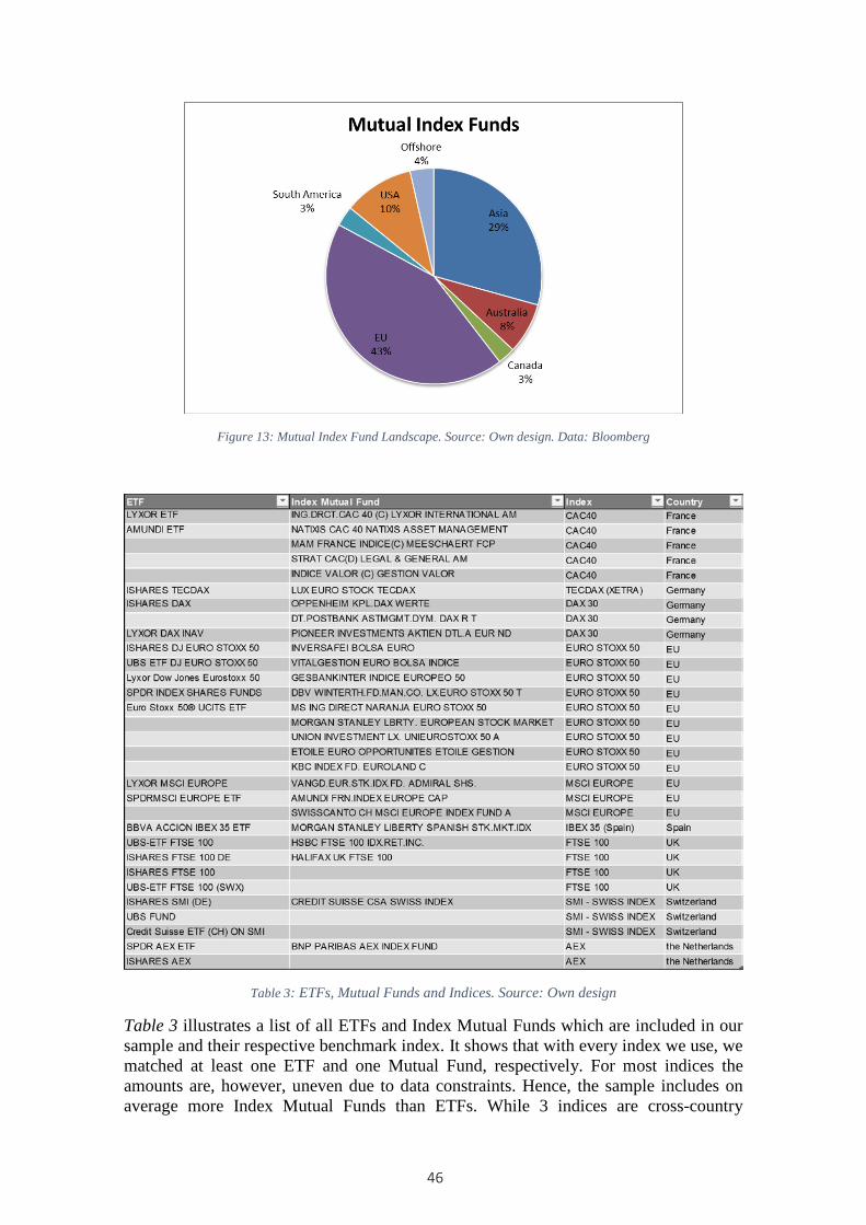
Figure 13: Mutual Index Fund Landscape. Source: Own design. Data: Bloomberg

Table 3: ETFs, Mutual Funds and Indices. Source: Own design

Table 3 illustrates a list of all ETFs and Index Mutual Funds which are included in our sample and their respective benchmark index. It shows that with every index we use, we matched at least one ETF and one Mutual Fund, respectively. For most indices the amounts are, however, uneven due to data constraints. Hence, the sample includes on average more Index Mutual Funds than ETFs. While 3 indices are cross-country

46

diversified (MSCI Europe, EURO STOXX50, MSCI Developed Europe), our sample includes country indices from France (CAC40), Germany (DAX), Netherlands (AEX), Spain (Ibex35), England (FTSE 100) and Switzerland (SMI).

Data Type Our study deals with the development of prices of index tracker funds and their benchmarks over a fixed period of time. We therefore obtain price data from different points in time during this period and order them according to their observation time. The observed prices serve as basis for our calculation and can, due to their timeline characteristics, be referred to as time series data. It is, however, to point out that we are not basing our analysis on a single time series, but make use of several time series for Mutual Index Funds on the one hand, and several series for ETFs on the other. This gives us two separate panel sets of variables we aim to compare (Koop, 2006, pp. 9-11). To draw an accurate picture of the prices over time, we use the highest frequency data which exist for both ETFs and Mutual Index Funds, i.e. daily prices. Even though ETFs are stated intraday as well, such data are not only difficult to obtain over a longer period, but also not available for Mutual Index Funds.

Expense Ratios Hypotheses 6-8 relate to the Funds’ Total Expense Ratios (TER), therefore we collected TERs for every Fund by extracting the most recent values from the factsheets of the fund providers. In rare cases when this information was not provided, we obtained the latest ratio stated on Morningstar.

4.1.4. MSCI Europe

We decided to use MSCI Europe index as a representative index for the European market state. The MSCI Europe Index captures large and mid-cap representations across 16 Developed Markets countries in Europe4. With 436 constituents, the index covers approximately 85% of the free float-adjusted market capitalization across the European Developed Markets equity universe. Over last 10 years, the index had a 9,41% and 19,89% annualized return and standard deviation, respectively. It uses the MSCI Global Investable Market Indices (GIMI) Methodology in order “to provide exhaustive coverage of the relevant investment opportunity set with a strong emphasis on index liquidity, investability and replicability” (MSCI, 2013, p. 2). To adopt changes in the underlying equity market the index is reviewed quarterly in February, Mai, August and November. (MSCI, 2013, p. 1-2).

4.1.5. Time Horizon

The time horizon of this study is mainly determined by the inception date of the used Exchange Traded Funds. As a rather young investment instrument, ETFs had a growth phase in the beginning of the 21st century, but are still developing. In order to achieve a sufficient number of ETFs we set the start date for the observations at the end of 2006 and finalize the investigation at the end of 2012. We see this timeframe as sufficient, as it not only captures the recent development and to the date most competitive years between Mutual Index Funds and ETFs, but also gives us the chance to look at different states of the economy, since these five years cover the subprime mortgage crisis and the

4 Austria, Belgium, Denmark, Finland, France, Germany, Greece, Ireland, Italy, the Netherlands, Norway, Portugal, Spain, Sweden, Switzerland, and the UK.

47

ongoing European sovereign debt crisis. This leaves room for a discussion about tracking performance of the two fund types during different states of the market.

The following graph shows the development of the MSCI Europe over the investigated periods and gives an impression of the different states of the European economy. It also allows us to define a set of sub-periods that might be worth examining separately.

Figure 14: Development of the MSCI Europe Index 2006-2013. Source: Own design.

What Figure 14 tells us about the European economy in the past 6 years starts with a strong breakdown between the end of 2007 and the beginning of 2008, which can be explained as triggered by the subprime mortgage crisis. After hitting a low point in the beginning of 2009, a recovery period starts but doesn’t last very long, as the European debt crisis thwarts down the upturn in Europe. If we take the MSCI Europe as a representative Index for the European Economy, we see that the debt crisis doesn’t really resulted in a recession, but more in a stagnation which is, like the crisis itself, still ongoing. The fact that the EU doesn’t experience a born-and-bred recession, might be due to the fact, that even though the European crisis states face the latter, other states remain stable and absorb the downfall. In addition, several actions undertaken by the European Central Bank aim for stabilization of the EU.

4.1.6. Sub-Periods

Given our window from 2007-2013 and the trend in Figure 12 we can identify the following sub-periods:

Period 1: Jan. 2006 to Oct. 2007, ascending trend Period 2: Nov. 2007 to Feb. 2009, strong recession (subprime mortgage crisis) Period 3: Mar. 2009 to Jan. 2010, ascending trend (recovering phase) Period 4: Jan. 2010 to Jan 2013 stagnation (European sovereign debt crisis) To decide on the borderlines of the sub-periods, we considered the bottoms and peaks (min. and max.) of the index and related them to economic events to identify the relevant breaking points. We use these sub-periods as benchmarks to identify any possible relationship between tracking quality and different market states, i.e. we investigate if index trackers benefit from either bull or bear markets.

48

4.2. Data Treatment and Adjustment

Throughout the analysis part of this thesis we occasionally have to adjust the used data in order to align them with the respective tests.

Time Transformation In order to conduct regression analysis to investigate the relationship between Tracking Error and index return, we need to annualize Tracking Errors, which have the same the characteristics with a standard deviation or variance. According to Probability Theory in order to annualize a standard deviation, one has to use the formula

𝜎𝜎𝑎𝑎𝑛𝑛𝑛𝑛𝑎𝑎𝑎𝑎𝑎𝑎 = 𝜎𝜎𝑑𝑑𝑎𝑎𝑖𝑖𝑎𝑎𝑑𝑑 ∗ √𝐼𝐼

Equation 9: Transformation of standard deviation

where n is the number of observations throughout the respective year. The corresponding transformation of daily index returns is done by

𝑅𝑅𝑎𝑎𝑛𝑛𝑛𝑛𝑎𝑎𝑎𝑎𝑎𝑎 = (1 + 𝑅𝑅𝑑𝑑)𝑛𝑛 − 1

Equation 10: Transformation of Returns

It is important to note that Equation 9 assumes no correlation between subsequent returns, which is usually accepted in finance, if ln transformation is performed beforehand.

Avoiding Autocorrelation Since one of our chosen methods to calculate tracking error is based directly on returns, there is a potential threat of autocorrelation within the time series of return. Taking this into account, apart from using log returns, we undertake further necessary actions to avoid serial correlation which we discuss subsequent to the introduction of the respective Tracking Error estimate.

Moving Average While investigating outliers during Tracking Error analysis, we make use of the Moving Average (MA) of the time series. MA is calculated in order to smoothen out a time series by averaging the original data over a specified period n. In our case we calculate moving averages of fund returns. This helps us to identify whether there are certain outliers within a series that influence our regression when ran with the original returns. We transform the original series {rt}t=1T to a new series {rtMA}t=1T−n+1 by taking the arithmetic mean of a sub-series of n observations:

rtMA = 1n� ri

t+n−1

i=t

Equation 11: Moving Average

Where rtMA is the new series from Moving Average, over n observations and T as the total amount of observations from the original series (as you can see in 5.3.1 we use t=100 out of n=1825).

49

4.3. Statistics

4.3.1. Statistical Expression of Hypotheses

We reformulate or hypotheses from chapter 3, using the same statistical terms as we are using throughout our statistical tests and presentation of results. We present hypotheses further, where we use µ𝑀𝑀𝑀𝑀, µ𝐸𝐸𝐸𝐸𝑀𝑀 and µ𝐼𝐼𝑛𝑛𝑑𝑑𝐼𝐼𝐼𝐼 for the mean returns of Mutual Funds, ETFs and Indices respectively, 𝑇𝑇𝑇𝑇𝑀𝑀𝑀𝑀 and 𝑇𝑇𝑇𝑇𝐸𝐸𝐸𝐸𝑀𝑀 for the respective Tracking Errors and 𝑇𝑇𝑇𝑇𝑅𝑅 for the respective Total Expense Ratios. For hypotheses 7 and 8 we calculate Betas (𝛽𝛽𝑀𝑀𝑀𝑀𝐸𝐸𝐸𝐸𝑅𝑅 𝑇𝑇𝐼𝐼𝐼𝐼 𝛽𝛽𝐸𝐸𝐸𝐸𝑀𝑀𝐸𝐸𝐸𝐸𝑅𝑅) as correlation coefficients between Tracking Error and Total Expense Ratio.

Hypothesis 1

The average return difference between Mutual Index Funds and their benchmark index is equal to zero.

𝐻𝐻0: µ𝑀𝑀𝑀𝑀 − µ𝐼𝐼𝑛𝑛𝑑𝑑𝐼𝐼𝐼𝐼 = 0

𝐻𝐻𝑁𝑁: µ𝑀𝑀𝑀𝑀 − µ𝐼𝐼𝑛𝑛𝑑𝑑𝐼𝐼𝐼𝐼 ≠ 0

Hypothesis 2

The average return difference between Exchange Traded Funds and their benchmark index is equal to zero.

𝐻𝐻0: µ𝐸𝐸𝐸𝐸𝑀𝑀 − µ𝐼𝐼𝑛𝑛𝑑𝑑𝐼𝐼𝐼𝐼 = 0

𝐻𝐻𝑁𝑁: µ𝐸𝐸𝐸𝐸𝑀𝑀 − µ𝐼𝐼𝑛𝑛𝑑𝑑𝐼𝐼𝐼𝐼 ≠ 0

Hypothesis 3

The mean Tracking Error difference between Exchange Traded Funds and Mutual Index Funds is equal to zero.

𝐻𝐻0: 𝑇𝑇𝑇𝑇𝑀𝑀𝑀𝑀 − 𝑇𝑇𝑇𝑇𝐸𝐸𝐸𝐸𝑀𝑀 = 0

𝐻𝐻𝑁𝑁: 𝑇𝑇𝑇𝑇𝑀𝑀𝑀𝑀 − 𝑇𝑇𝑇𝑇𝐸𝐸𝐸𝐸𝑀𝑀 ≠ 0

Hypothesis 4

For ETFs there is no correlation between mean Tracking Error and the European economy.

𝐻𝐻0: 𝛽𝛽𝐸𝐸𝐸𝐸𝑅𝑅𝐸𝐸𝐸𝐸𝐸𝐸𝐸𝐸𝐸𝐸 = 0

𝐻𝐻𝑁𝑁: 𝛽𝛽𝐸𝐸𝐸𝐸𝑅𝑅𝐸𝐸𝐸𝐸𝐸𝐸𝐸𝐸 ≠ 0

Hypothesis 5

For MIFs there is no correlation between mean Tracking Error and the European economy.

𝐻𝐻0: 𝛽𝛽𝐸𝐸𝐸𝐸𝑅𝑅𝐸𝐸𝐸𝐸𝐸𝐸𝐸𝐸𝐸𝐸 = 0

50

𝐻𝐻𝑁𝑁: 𝛽𝛽𝐸𝐸𝐸𝐸𝑅𝑅𝐸𝐸𝐸𝐸𝐸𝐸𝐸𝐸 ≠ 0

Hypothesis 6

The difference of mean Total Expense Ratio between Exchange Traded Funds and Mutual Index Funds is equal to zero.

𝐻𝐻0: 𝑇𝑇𝑇𝑇𝑅𝑅𝑀𝑀𝑀𝑀 − 𝑇𝑇𝑇𝑇𝑅𝑅𝐸𝐸𝐸𝐸𝑀𝑀 = 0

𝐻𝐻𝑁𝑁: 𝑇𝑇𝑇𝑇𝑅𝑅𝑀𝑀𝑀𝑀 − 𝑇𝑇𝑇𝑇𝑅𝑅𝐸𝐸𝐸𝐸𝑀𝑀 ≠ 0

Hypothesis 7

There is no correlation between Total Expense Ratio and Mutual Index Fund Tracking Error.

𝐻𝐻0: 𝛽𝛽𝐸𝐸𝐸𝐸𝐸𝐸𝐸𝐸𝑅𝑅 = 0

𝐻𝐻𝑁𝑁: 𝛽𝛽𝐸𝐸𝐸𝐸𝐸𝐸𝐸𝐸𝑅𝑅 ≠ 0

Hypothesis 8

There is no correlation between Total Expense Ratio and Exchange Traded Fund Tracking Error.

𝐻𝐻0: 𝛽𝛽𝐸𝐸𝐸𝐸𝐸𝐸𝐸𝐸𝑅𝑅 = 0

𝐻𝐻𝑁𝑁: 𝛽𝛽𝐸𝐸𝐸𝐸𝐸𝐸𝐸𝐸𝑅𝑅 ≠ 0

4.3.2. Calculating Returns

We want to calculate Tracking Errors as described in chapter 3. Therefore we first have to transform our daily observed prices to returns, which can simply be done by

𝑃𝑃𝑡𝑡 = �𝑃𝑃𝑡𝑡+1𝑃𝑃𝑡𝑡

� − 1

Equation 12: Calculation of Returns

This formula represents simple net return of an asset for a holding period between t and t+1..

However, it is convenient for financial time series analysis to make use of the natural logarithms of the return series (log return continuously compound return), which is calculated as

𝑃𝑃𝑡𝑡 = 𝑇𝑇𝐼𝐼 �𝑃𝑃𝑡𝑡+1𝑃𝑃𝑡𝑡

�

Equation 13: Calculation of Logarithmic Returns

Investigating a time series, i.e. a series of data from different points in time, Equation 13 is favorable method due to the symmetric and additive characteristic of the logarithms which are assumed to be approximately normally distributed and independent (no autocorrelation), while the arithmetic returns indicate a dependent relationship (Adelmeyer & Warmuth, 2005, pp. 55–56).

51

The sum of log returns over the whole time horizon gives us the total return for ETF, Mutual Index Fund and benchmark index and serves as the basis for our analysis.

4.3.3. Volatility

The volatility of an investment is used to express its risk exposure and is calculated as the standard deviation of the daily returns (Rompotis, 2005, p. 10). The volatility of the different time series for every fund and index is therefore calculated as

𝑆𝑆2 = � 1𝐸𝐸−1

∑ (𝑃𝑃𝑇𝑇 − 𝑃𝑃�𝑇𝑇)𝑇𝑇𝑇𝑇=1

Equation 14: Volatility of a return series

where T is the number of observations, 𝑃𝑃𝑡𝑡 the observed value at time t and �̅�𝑃 the mean of the observations of the respective ETFs, Mutual Index Fund or Index.

4.3.4. Correlation Analysis

To be able to answer hypothesis 4-5 and 7-8 we need to find possible correlations between fund expenses and Tracking Error. The correlation coefficient measures the direction and strength of the linear dependence between to two variables, i.e. in our case between Total Expense Ratio and Tracking Error. The correlation function is defined as

𝑃𝑃𝐼𝐼,𝑑𝑑 = 𝐶𝐶𝐶𝐶𝐶𝐶(𝑋𝑋,𝑌𝑌)�𝑁𝑁𝑎𝑎𝑉𝑉(𝑋𝑋)𝑁𝑁𝑎𝑎𝑉𝑉(𝑌𝑌)

Equation 15: Correlation Function

where X and Y are the investigated variables. For our sample where {(𝐼𝐼𝑖𝑖,𝑦𝑦𝑖𝑖)}𝑖𝑖=1𝑁𝑁 are available the correlation can be written as

rx,y = ∑ (𝐼𝐼𝑖𝑖− �̅�𝐼)(𝑑𝑑𝑖𝑖−𝑁𝑁𝑖𝑖=1 𝑑𝑑�)

�∑ (𝐼𝐼𝑖𝑖− �̅�𝐼)2 ∑ (𝑑𝑑𝑖𝑖−𝑑𝑑�𝑁𝑁𝑖𝑖=1

𝑁𝑁𝑖𝑖=1 )²

Equation 16: Extended Correlation Function

with �̅�𝐼 and 𝑦𝑦� as the respective sample mean ( ∑ 𝐼𝐼𝑖𝑖 𝑁𝑁𝑖𝑖=1 and ∑ 𝑦𝑦𝑖𝑖 𝑁𝑁

𝑖𝑖=1 ). (Tsay, 2005, p. 26)

The correlation between two variables always takes a value between -1 and 1, where correlation increases with the strength of deviation from 0, i.e. 1 indicates perfect positive association, -1 perfect negative association and 0 an uncorrelated relationship.

T-Ratio To test the null hypothesis for the Pearson’s correlation coefficient as stated above, i.e. to test if our sample means are linearly independent, we calculate the t-ratio as

t = r√N−2�1−r²

Equation 17: T-Ratio

52

where r is the correlation coefficient, N is the sample size and N – 2 are the degrees of freedom (df). (Howell, 2009, p. 272)

4.3.5. Regression Analysis

We make use of a simple regression analysis, in order to further explain the relationship between fund return and index return. Therefore we regress the return 𝑃𝑃𝑓𝑓𝑖𝑖 of every fund against the return 𝑃𝑃𝑏𝑏𝑖𝑖 of its benchmark index. We use the same time-series regression model as Rompotis (2005, p. 12). We use the same time-series regression model as Rompotis (2005, p. 12). We intend to gain information about the funds’ portfolio sensitivity towards index movements and therefore about their replication accuracy.

𝑃𝑃𝑓𝑓𝑖𝑖 = 𝛼𝛼𝑖𝑖 + 𝛽𝛽𝑖𝑖𝑃𝑃𝑏𝑏𝑖𝑖 + 𝜀𝜀𝑖𝑖

Equation 18: Simple Regression Function

In Equation 18, 𝛼𝛼𝑖𝑖 is the independent constant and represents the return a fund portfolio achieves independently from the index return. Since we exclusively investigate passively managed funds, this value is expected, and if analogous management is used, the value should be insignificantly small. Therefore, most of the return should be explained by the fund portfolios 𝛽𝛽𝑖𝑖, which if the portfolio is successfully managed should be close to 1 and therefore highly correlated with the index returns. 𝜀𝜀𝑖𝑖 represents the residuals of the respective fund, which are not explained by the model.

Assumptions There are three assumptions that have to be tested first in order to verify the suitability of regression analysis:

1. 𝑇𝑇(𝜀𝜀𝑖𝑖) = 0 𝜀𝜀 has a mean of zero for all i 2. 𝑇𝑇(𝜀𝜀𝑖𝑖)2 = 𝜎𝜎𝜀𝜀2 the variance is constant for all 𝜀𝜀𝑖𝑖 3. 𝑇𝑇�𝜀𝜀𝑖𝑖𝜀𝜀𝑗𝑗�

2= 0, 𝑃𝑃 ≠ 𝑗𝑗 there is no correlation across observations

(Autocorrelation) (Cottrell, 2003, p. 1)

We carefully evaluate these assumptions before regression is made. We test if residuals are normally distributed by analyzing the Q-Q plot and running a Kolmogorov-Smirnov test. Further, autocorrelation is tested by plotting the standardized residuals against predicted values and calculating Durbin-Watson statistics. The results of the tests are presented and discussed in chapter 5.

T-statistic Simultaneously to the correlation coefficient, after estimating the size of β we apply t-statistics to test the level of significance of the hypothesis 𝐻𝐻0: 𝛽𝛽 = 0 against 𝐻𝐻𝑁𝑁: 𝛽𝛽 ≠ 0 to gain affirmation that the regression is capable of explaining the relationship between index and fund portfolio within a certain confidence interval, i.e. we are testing if the explanatory variable has an actual effect on the depended variable. The t-statistic is calculated by

𝑇𝑇′ = 𝛽𝛽𝑆𝑆𝑏𝑏

Equation 19: T-Statistics

53

where β as our beta estimate and 𝑆𝑆𝑏𝑏 as the standard deviation of beta. If beta estimates are large relative to its standard deviations and therefore the t-value is large (relative to its critical value from the Student-t distribution), we can reject 𝐻𝐻0 and accept 𝐻𝐻𝑁𝑁. While executing t-tests in Ms Excel, we obtain a P-Value which determines the relative size of the t-statistic, i.e. for 95% confidence interval, if P ≤ 5% we can reject 𝐻𝐻0. (Koop, 2006, pp. 79–81)

4.3.6. Tracking Error Estimates

To compare tracking accuracy between ETFs and Mutual Index Funds, we make use of different methods to calculate Tracking Errors. Besides the widely used definition of TE as the standard deviation of return differences, we use two alternative estimates, also utilized by Frino and Gallagher when investigating the tracking of S&P 500 Index Funds. (2001, pp. 8–9)

𝑻𝑻𝑬𝑬𝟏𝟏 Our first Tracking error is calculated using the standard error of the regression from Equation 20. The standard error is calculated by

𝑇𝑇𝑇𝑇1 = 𝑆𝑆𝑆𝑆𝑅𝑅 = �∑(𝑌𝑌𝑖𝑖−𝑌𝑌𝚤𝚤� )²𝑛𝑛−2

= �∑𝜀𝜀𝑖𝑖²𝑛𝑛−2

Equation 20: Tracking Error 1

where the sum of the squared residuals divided by n – 2 degrees of freedom (n = number of observations).

𝑇𝑇𝑇𝑇1 was suggested by Roll (1992) as an idea to investigate managers’ performance. Their goals are: to produce positive returns over a benchmark, keep TE volatility low relatively to the index, determine the exact composition of the particular portfolio, which could dominate the benchmark and possess low TE by putting constraints on a beta. Thus, 𝑇𝑇𝑇𝑇1is a good measure of managers’ performance, but it is also useful for analyzing tracking performance.

𝑻𝑻𝑬𝑬𝟐𝟐 The standard methodology to calculate TE as introduced in chapter 3, is the standard deviation of return differences. The standard deviation S is defined has the square root of the variance S² and calculated as

𝑆𝑆2 = 1𝐸𝐸−1

∑ (𝐼𝐼𝑡𝑡 − �̅�𝐼𝑡𝑡)𝐸𝐸𝑡𝑡=1 ²

Equation 21: Variance of Return Differences

In Equation 21, 𝐼𝐼𝑡𝑡 is the return difference 𝑃𝑃𝑡𝑡𝑀𝑀𝑎𝑎𝑛𝑛𝑑𝑑 − 𝑃𝑃𝑡𝑡𝐼𝐼𝑛𝑛𝑑𝑑𝐼𝐼𝐼𝐼 and the mean �̅�𝐼 is defined as

�̅�𝐼 = 1𝐸𝐸∑ 𝐼𝐼𝑡𝑡𝐸𝐸𝑡𝑡=1

Equation 22: Mean of Return Differences

where the sum of the observation values divided by their count. Then, our second measure for Tracking Error can be simply expressed as

54

𝑇𝑇𝑇𝑇2 = �𝑆𝑆2

Equation 23: Tracking Error 2

Since 𝑇𝑇𝑇𝑇2 is popular and frequently used in academic studies (cf. inter alia Roll, 1992; Rudolf et al., 1999; Frino & Gallagher, 2001, Aber et al., 2009 and Hwang & Satchel, 2001), we focus on 𝑇𝑇𝑇𝑇2 methodology is also the common approach for the funds and for rating agencies like Morningstar.com (Morningstar, 2013b).

Pope and Yadav (1994) note that calculating annual 𝑇𝑇𝑇𝑇2 based on daily returns could bias it due to serial autocorrelation of returns. However, we adjusted our returns in cases of serial correlation by using lag returns. We checked for autocorrelation using Durbin-Watson statistics for the obtained daily returns. In addition, we drew PACF (partial autocorrelation function charts) and determined the correct lag needed for the model in case of autocorrelation. Next, we adjusted our returns using the correct lag and performed regression using dynamic model 𝑌𝑌𝑡𝑡 = 𝛼𝛼 + ∑ 𝛽𝛽𝑖𝑖𝑋𝑋𝑡𝑡−𝑖𝑖𝑖𝑖=1 + 𝜀𝜀𝑡𝑡 with the stated lag.

𝑻𝑻𝑬𝑬𝟑𝟑 The third TE estimate is the average absolute return difference, i.e. we calculate the daily average of the absolute return difference, 𝐼𝐼𝑡𝑡 = 𝑃𝑃𝑡𝑡𝑀𝑀𝑎𝑎𝑛𝑛𝑑𝑑 − 𝑃𝑃𝑡𝑡𝐼𝐼𝑛𝑛𝑑𝑑𝐼𝐼𝐼𝐼 as

𝑇𝑇𝑇𝑇3 =∑ |𝐼𝐼𝑡𝑡| 𝐸𝐸𝑡𝑡=1

𝑇𝑇

Equation 24: Tracking Error 3

𝑇𝑇𝑇𝑇3 was developed by Rudolf et al. (1999) who estimated that 𝑇𝑇𝑇𝑇3 could give better risk descriptions to investors if performance fees of fund managers are linear.

4.3.7. Two-Sample t-test

To compare the means of two time series (i.e. to explore significant differences), we use a two-sample t-test. Since we are interested in any potential difference, our hypothesis for this test is 𝐻𝐻0: 𝜇𝜇𝐼𝐼 − 𝜇𝜇𝑑𝑑 = 0 and thus 𝐻𝐻𝑁𝑁: 𝜇𝜇𝐼𝐼 − 𝜇𝜇𝑑𝑑 ≠ 0. As our series have unequal variances, we use the heteroscedastic t-test (or unequal variance t-test). The basis for this t-test is the estimated standard deviation of the sample difference in sample means. Since, the standard deviation of the population is unknown, it is estimated by the two samples’ standard deviation:

�𝑆𝑆12

𝑛𝑛1+ 𝑆𝑆22

𝑛𝑛2

Equation 25: Two-Sample Standard Deviation

We standardize the estimates by dividing it by the standard error, which gives us the two-sample t-test

55

𝑇𝑇′ = 𝐼𝐼1����−𝐼𝐼2����

�𝑆𝑆12

𝑛𝑛1+𝑆𝑆2

2

𝑛𝑛2

Equation 26: Two-Sample T-test

where 𝐼𝐼1��� − 𝐼𝐼2��� is the difference between the observed estimates and 𝐼𝐼 the respective number of the observations of series 1 and 2. (Moore, 1996, p. 469)

4.4. Regressions with categorical dependent variable

Categorizing variables During our analysis of MIF and ETF tracking performance, we decided to construct pairs, where an ETF and MIF are tracking the same index. For the list of pairs, please see Appendix 1. Afterwards, we calculated absolute return differences (ARD) between a benchmark index and a MIF for each period. The same procedure was repeated for an ETF as well. Next, in order to compare the ARD of an ETF and a MIF in a matched pair (both ETF and MIF track the same index), we categorized our ARD by “1” if tracking performance of ETF is better during the respective period and “0” if tracking performance of MIF is better. We obtained a categorical variable for the period of 2007 to the end of 2012 by using monthly observations (resulting in 15 pairs with 72 observations each).

We make use of logistic regression as an attempt to explain the phenomenon when over a period of time ETFs performed better tracking compared to MIF, and vice versa. We chose explanatory variables to find out whether they have a positive or negative impact on our two fund types. In fact, as we will see throughout our analysis, there are certain periods during which return differences of ETFs are lower than those of MIFs and the other way around. We decided to research this phenomenon, using index returns 𝑅𝑅𝑖𝑖 and volatility 𝜎𝜎𝑖𝑖 as explanatory variables as those are universal tools, which give good essential knowledge about the index as well as the current state of the market.

In order to study a categorical variable which has only two values (MIF or ETF), three options exist: Linear Probability Model (LPM), probability model (probit) and logistic regression (logit).

4.4.1. Linear Probability Model (LPM)

LPM is a special case of binomial regression, where the dependent variable takes values which are either 0 or 1. The relationship of variables is simple, which allows the model to be fitted by OLS. The model is

𝑃𝑃(𝑌𝑌 = 1|𝐼𝐼) = 𝐼𝐼`𝛽𝛽

Equation 27: LPM model

where P is the probability.

The method of fitting OLS with a categorical dependent variable has significant drawbacks. Estimated coefficients would generate probabilities outside the unit interval and conditions for residuals will not be accepted. For this reason LPM is of limited usage and other models such as logit or probit are commonly used. (Hahn & Sover, 2010)

56

4.4.2. Probit model

The aim of the model is to calculate the probability of an event with special characteristics of being categorized in a group with similar characteristics. Categorizing an event into a group usually requires the probability to be more than 0,5. Probit is used to model ordinal or binary outcome variables. In the probit model, the inverse standard normal distribution of the probability is modelled as a linear combination of the predictors. It is similar to logistic regression and is estimated using the standard maximum likelihood procedure (regression). The model is:

𝑃𝑃(𝑌𝑌 = 1|𝐼𝐼) = Ф(𝐼𝐼`𝛽𝛽)

Equation 28: Probit model

where P is probability and Ф is Cumulative Distribution Function (CDF) of a Normal distribution.

The probit model standardises all 𝛽𝛽 coefficients to z values on a CDF of Normal distribution. Thus, interpretations of the results are limited to z scores. Other interpretation requires calculation of probabilities, which are limited to a specific observation case. Therefore, we decide to implement a more common approach and to use a logit model for the convenience of our interpreting results. (Hahn & Sover, 2010)

4.4.3. Logit model

The logit model allows to model categorical variables in a way similar to OLS. Logistic regression has become the most used technique in the class of generalized linear models due to its simplicity regarding interpretation. In logistic regression, the function is ln transformed. The researcher uses the natural logarithm of the odds that a given event will occur. In OLS, parameters are estimated using the method of least squares by minimizing the sum of squared deviations of predicted values from observed values. For logistic regression, least squares estimation is not capable of producing minimum variance unbiased estimators for the actual parameters. Instead, maximum likelihood estimation is used. (Czepiel, 2002, pp. 2-3)

The model is

𝑇𝑇𝐼𝐼 �𝑃𝑃(𝐼𝐼)

1 − 𝑃𝑃(𝐼𝐼)� = �𝐼𝐼𝑖𝑖𝑖𝑖𝛽𝛽𝑖𝑖 ; 𝑃𝑃 = 1,2, … ,𝑁𝑁

𝑖𝑖

𝑖𝑖=0

Equation 29: Logit model

where � 𝐸𝐸(𝐼𝐼)1−𝐸𝐸(𝐼𝐼)

� are the odds.

In our case we decided to use two independent variables – index returns and volatility, simultaneously and separately in order for the model to get higher goodness of fit levels.

57

Logit model interpretations The model is easy to interpret as it provides an Odds Ratio (OR) and a probability for a special event.

𝑂𝑂𝑅𝑅 =𝑑𝑑𝐼𝐼𝐼𝐼𝑑𝑑𝐼𝐼+1𝑑𝑑𝐼𝐼𝐼𝐼𝑑𝑑𝐼𝐼

=𝐼𝐼𝛽𝛽𝑜𝑜+𝛽𝛽1(𝐼𝐼1+1)

𝐼𝐼𝛽𝛽𝑜𝑜+𝛽𝛽1𝐼𝐼1= 𝐼𝐼𝛽𝛽1

Equation 30: Odds Ratio (OR)

𝑃𝑃(𝑌𝑌 = 1|𝐼𝐼) = 𝑇𝑇(𝑌𝑌) = 𝐼𝐼𝛽𝛽𝑜𝑜+𝛽𝛽1𝑥𝑥1

1+𝐼𝐼𝛽𝛽𝑜𝑜+𝛽𝛽1𝑥𝑥1= 𝐼𝐼𝛽𝛽1 ; 0 < 𝑇𝑇(𝑌𝑌)<1

Equation 31: Probability for a specific event

Logit model: Odds Ratio Odds are the ratio of the probabilities, that event x would occur (𝑃𝑃(𝐼𝐼)) and would not occur (1 − 𝑃𝑃(𝐼𝐼)). The odds ratio, determined in logit regression is the ratio of the odds, for the event (Y=1) if x increases by one unit to the odds of event (Y=1) when x remains constant. It is found as 𝐼𝐼𝛽𝛽1, where 𝛽𝛽1 is the slope in the logistic regression equation. OR could be interpreted as if one event has a better chance over another event, if one would add additional unit to x, ceteris paribus. For example, in our case if slope 𝛽𝛽1 is positive and OR for return is equal to 1,3, we will state that for every unit increase in returns (e.g. by 0,01%) the odds that ETFs would track better than MIF increase by 1,3 times, keeping other things constant. (Moore et al. 2011, pp. 17-8 – 17-12)

Logit model: Probability for a specific event In addition to the odds ratio, we can add a probability for a specific event as for example the probability of ETF tracking better than MIF if index returns change from 11 to 12 per cent, keeping other things constant. (Moore et al. 2011, pp. 17-8 – 17-11)

Logit model: goodness of fit characteristics We implemented a specific goodness of fit procedures for the model to confirm that model fits the data correctly. We used measures:

• Percentage of correct prediction, which identifies how many results were correctly predicted by our model;

• Log likelihood estimation in order to compare models fit; • Hosmer and Lemeshow Test, which accesses the data fit and calculates how

observed events match expected events. It is favourable to have high p-values for this test, because p-values will show that the model fits the data correctly.

• Wald’s ratio and its significance, which is similar to p-value in OLS.

We used pseudo R², which is similar to OLS R² but computed under the restrictions of the logit model. Specifically, we paid attention to R² of Cox & Snell (a non-standardized Cox & Snell R² may not reach 1 at maximum levels) and Nagelkerke (a standardized version of Cox & Snell R² could be between 0 and 1). (SPSS, 2012)

Logit or probit Long (1997, p. 83) notes that the choice between the logit and probit models is largely one of applicability, as the results are generally indistinguishable.

58

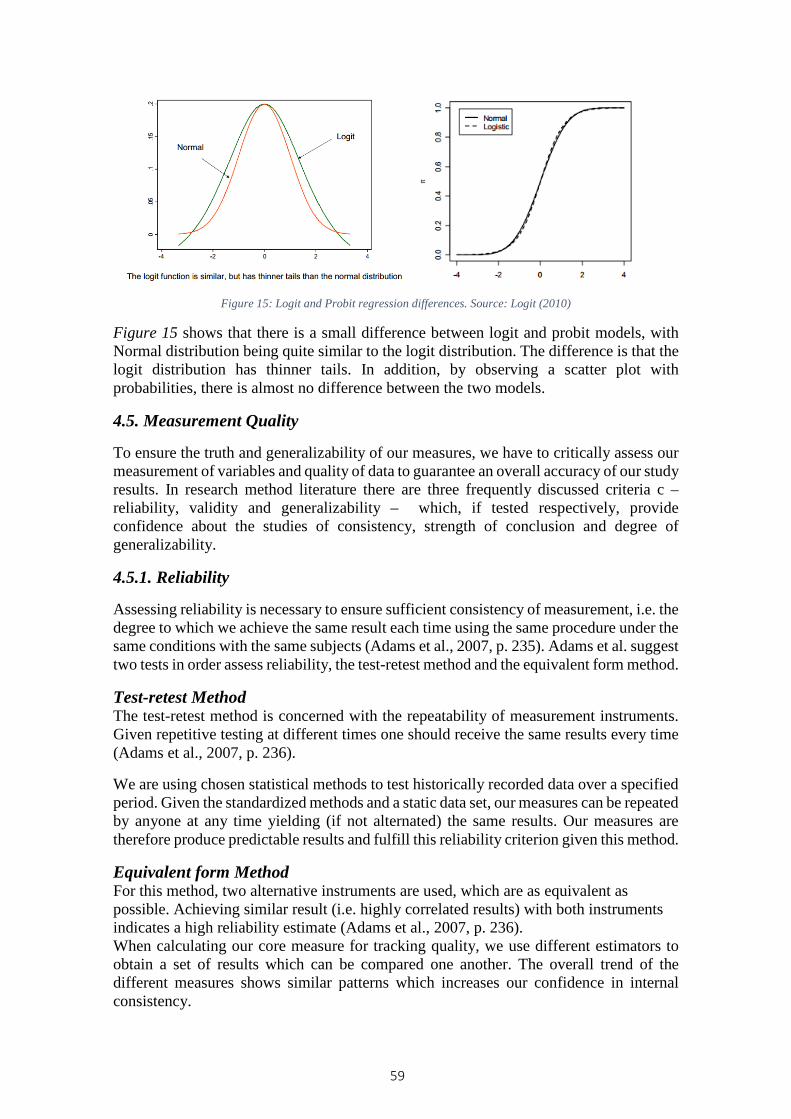
Figure 15: Logit and Probit regression differences. Source: Logit (2010)

Figure 15 shows that there is a small difference between logit and probit models, with Normal distribution being quite similar to the logit distribution. The difference is that the logit distribution has thinner tails. In addition, by observing a scatter plot with probabilities, there is almost no difference between the two models.

4.5. Measurement Quality

To ensure the truth and generalizability of our measures, we have to critically assess our measurement of variables and quality of data to guarantee an overall accuracy of our study results. In research method literature there are three frequently discussed criteria c – reliability, validity and generalizability – which, if tested respectively, provide confidence about the studies of consistency, strength of conclusion and degree of generalizability.

4.5.1. Reliability

Assessing reliability is necessary to ensure sufficient consistency of measurement, i.e. the degree to which we achieve the same result each time using the same procedure under the same conditions with the same subjects (Adams et al., 2007, p. 235). Adams et al. suggest two tests in order assess reliability, the test-retest method and the equivalent form method.

Test-retest Method The test-retest method is concerned with the repeatability of measurement instruments. Given repetitive testing at different times one should receive the same results every time (Adams et al., 2007, p. 236).

We are using chosen statistical methods to test historically recorded data over a specified period. Given the standardized methods and a static data set, our measures can be repeated by anyone at any time yielding (if not alternated) the same results. Our measures are therefore produce predictable results and fulfill this reliability criterion given this method.

Equivalent form Method For this method, two alternative instruments are used, which are as equivalent as possible. Achieving similar result (i.e. highly correlated results) with both instruments indicates a high reliability estimate (Adams et al., 2007, p. 236). When calculating our core measure for tracking quality, we use different estimators to obtain a set of results which can be compared one another. The overall trend of the different measures shows similar patterns which increases our confidence in internal consistency.

59

4.5.2. Validity

Validity describes the strength of relationship between our actual measures and the purpose of the measures and thus the strength of our conclusions, inferences and proposition we derive from them. Validity therefore is a necessary addition to reliability as even if measured consistently, our finds are only useful if they represent what we actually want to measure. Here we can mainly be distinguish between internal and external validity. While internal threats affect the causality of the relationship between dependent and independent variable and external threats affect the generalizability to other settings and situations. (Adams et al., 2007, p. 237)

Internal Validity

Our results could be biased by random influences due to differences in characteristics of our selected sample. We address this problem by considering and treating alternative influences to our results by concretizing our sample selection using a set of criteria as defined in 4.1.1. in order to avoid uncontrolled influences. We further use a longer timeframe covering different states of the market to avoid snapshot effects and be able to explore results against the background of different external influences. Different methods to test the strength of relationship between explanatory and independent variable as well as for the significance of results will further help us to validate our findings from a statistical perspective.

External Validity

To be able to generalize our findings, our study needs to be externally valid. Threats to external validity evolve mainly from undesired influences on respondents which are not accounted for during the assessment. Our data consists of prices which is determined by the market behavior over time incorporating all influencing variables on market characteristics which we don’t bias our time series but rather reflect the true reality as close as possible. However, yet again our sample could be biased by uncontrolled patterns in the number respondents (respondents in our case are funds to which we have sufficient data excess). We therefore use the highest possible sample within our sample criteria and across different indices to achieve satisfactory external validity

4.5.3. Generalizability

In order to make our research useful for application by the target audience and for further researches, we need to make sure that we can generalize our results beyond our study to the population (Adams et al., 2007, p. 239; Saunders, 2009, p. 158). Since our goal is not to study the relationship between one pair of funds, but rather the European index fund industry as a whole, we need to make sure if and which of our findings can be generalized to the population. We take a careful and conservative position towards our findings and the conclusions we draw from them. Therefore, we retest especially weak relationships by altering the variables, e.g. removing outliers. If outliers are identified to be the stimulus threshold to make a result statistically significant, we take them out of consideration as such results would strongly weaken the ability to generalize. If statistics or other indicators lead to doubtfulness of generalizability, we will point out the results in question correspondingly.

60

5. Results and Analysis Throughout chapter 5 we will first present and describe our sample data using descriptive statistics. Calculating descriptive statistics provides us with the necessary data to answer the first two hypotheses. We then report the results of our analysis regarding Tracking Errors and Expense Ratios and, based on the results answer the remaining hypotheses and discuss them respectively in relation with the literature reviewed in chapter 3. We conclude the chapter with a brief summary of our hypothesis outcomes..

5.1. Chapter Outline

Figure 16: Framework of research analysis. Source: own design.

Figure 16 shows an outline of the Analysis. To investigate the tracking performance, we first calculate returns and return differences (to the benchmark index) for all funds. The descriptive statistics of the return differences will tell us, if the average returns of the funds deviate from the indices returns. In order to explain possible differences of tracking performance of the two fund types, we run a dummy regression using index returns and index volatility as explanatory variables. In the second part of the chapter we calculate different estimates for Tracking Error for MIFs and ETFs. We compare those estimates over the whole time horizon, on an annual basis as well as throughout sub-periods as determined by the two recent market crises. We conclude the analysis by searching for a relationship between Tracking Error and Total Expense Ratio.

61

5.2. Comprehensive Descriptive Statistics

Table 4 gives a summary of average annualized returns and standard deviation of ETFs, Mutual Index Funds (MIF) and the respective benchmark indices. Due to the amount of used funds, we do not state the respective values for each fund but rather merge the values for funds that track the same index.

The mean returns for all ETFs, Mutual Index Funds and indices are -1,71%, -1,0% and -1,2% respectively. We see that ETFs and MIFs mean return are very close to the index, with a remaining difference between ETF and index amounting to -71 bps and to +20 bps between MIF and index. The numbers indicate that ETFs and MIFs deliver approximately the same returns as the benchmarks with MIF performing slightly better. Since the calculated differences in return are very small, we focus on the t-statistics in order to determine whether they have significant implications. In fact, the return differences between funds and benchmarks vary insignificantly from zero as the t-statistics show in Appendix 2. The same applies to the difference between ETF and MIF returns as it can be seen in Appendix 3.

The descriptive statistics of the respective returns provide us with sufficient information to answer hypothesis 1 and 2.

We recall hypothesis 1 and 2:

Hypothesis 1

The average return difference between Mutual Index Funds and their benchmark index is equal to zero. 𝐻𝐻0: µ𝑀𝑀𝑀𝑀 − µ𝐼𝐼𝑛𝑛𝑑𝑑𝐼𝐼𝐼𝐼 = 0

𝐻𝐻𝑁𝑁: µ𝑀𝑀𝑀𝑀 − µ𝐼𝐼𝑛𝑛𝑑𝑑𝐼𝐼𝐼𝐼 ≠ 0

Table 4: ETF, MIF and Index returns averaged 2006-2013

Name Observations(each fund)

Type ETF MIF Index ETF MIF IndexAEX -0,035 -0,034 -0,035 0,248 0,247 0,247 1825CaC40 -0,026 -0,029 -0,001 0,257 0,266 0,259 1825DAX 30 0,046 0,043 0,053 0,260 0,268 0,261 1680EURO STOXX 50 -0,045 -0,023 -0,044 0,273 0,254 0,258 1825FTSE 100 -0,037 0,009 -0,003 0,266 0,227 0,236 1762IBEX 35 -0,087 -0,060 -0,089 0,289 0,275 0,289 1597MSCI EUROPE -0,012 -0,017 -0,019 0,239 0,262 0,292 1689SMI - SWISS INDEX -0,002 0,008 -0,015 0,196 0,199 0,201 1825TECDAX (XETRA) 0,043 0,014 0,047 0,300 0,254 0,279 1825Average -0,017 -0,010 -0,012 0,259 0,250 0,258

Mean Return (Annual) St. Dev. (Annual)

62

Hypothesis 2

The average return difference between Exchange Traded Funds and their benchmark index is equal to zero.

𝐻𝐻0: µ𝐸𝐸𝐸𝐸𝑀𝑀 − µ𝐼𝐼𝑛𝑛𝑑𝑑𝐼𝐼𝐼𝐼 = 0

𝐻𝐻𝑁𝑁: µ𝐸𝐸𝐸𝐸𝑀𝑀 − µ𝐼𝐼𝑛𝑛𝑑𝑑𝐼𝐼𝐼𝐼 ≠ 0

The results of our return test as presented in table 3 show small differences in returns between funds and index, where MIF returns seem to be slightly higher and ETF returns lower than index returns. However, given the t-statistics, for our sample and timeframe we accept 𝐻𝐻0 for both hypotheses since the mean daily return differences from 2006 to 2013 between ETF and benchmark and between Mutual Index Fund and benchmark did not significantly deviate from zero. This implies that there is neither underperformance nor outperformance of ETF or MIF. We therefore reject the alternative hypotheses 𝐻𝐻𝑁𝑁 for ETFs and MIFs and state that on average, both fund models sufficiently approximate index returns, i.e. there is no significant overperformance or underperformance. These findings will also be verified by the results of the preparative regression analysis in part 5.3.1.

These results meet our expectations of passive index tracker funds and are in accordance with the findings of Rompotis (2005), who found neither significant return differences between ETF, index and MIF, nor any excess returns relative to the index. Svetina and Wahal (2008) also found ETFs and Mutual Index funds to be statistically indistinguishable when compared gross of fees. At the same time the results back Agapovas’ suggestion of ETFs and MIFs being substitutes to a certain degree (Agapova, 2011). However, other existing literature suggests average underperformance of Index Funds. Blitz et al. (2010), for instance, found underperformance of an average 84 bps in passive index funds in general (ETF and MIF). Given the insignificance of return differences we cannot confirm this trend for our sample of Europe trackers.

5.3. Analysis of return differences

To reveal any possible return differences due to seasonality we compared absolute return differences by constructing 15 pairs of dummy variables, with each pair ranging within the same index. Further, we obtained an average for all pairs in one month. Figure 17 shows the performance measured by absolute return differences for the chosen European funds.

63

Figure 17: Return difference comparison among ETFs and MIFs, values closer to 1 indicate better performance of

ETFs, closer to 0 – better performance of MIFs; Source: own design.

The descriptive statistics for the obtained data are as follows:

• Mean 0,40; median 0,40; geometric mean 0,40. All means are 0,40, which shows that the data are normally distributed and centered at one point. The meaning of 0,40 is that MIFs performed better since this number is closer to zero. Although the mean is 0,40, we cannot generalize this finding, because the chosen 15 pairs do not represent the whole number of funds used in analysis of TE throughout 5.2.2. and 5.2.3., because in these sections, we used 43 funds (21 ETFs and 22 MIFs) and in the above analysis only 30 funds (15 ETFs and 15 MIFs).

• Standard deviation is 0,031; max 0,49; min 0,32, skewness 0. This shows that the data are approximately log-normally distributed (there are no negative observations) and are not varying significantly with time, which is also clearly illustrated in Figure 17.

In a nutshell, we tried to find any seasonality of MIF and ETF tracking performance, but have not obtained any proof of this effect throughout our examination of the selected 30 funds from 2007 untill 2013. Frino and Gallagher (2001) tried to find a seasonality effect of tracking performance for ETFs only and revealed that tracking performance is closely connected with dividends. In our case the graph shows a very slow tendency to better performance of ETFs in the future. We can therefore complement the evidence from hypothesis 1 and 2 with the fact that return differences for both instruments remain constant in the short as well as in the long term.

5.3.1. Summary of Results: Logistic regression

After performing logistic regression, we found no evidence that index returns and/or volatility could influence the phenomenon, where in some periods ETFs perform better replication over MIFs or contrariwise. Our results were not significant or showed no dependency between the explanatory variables used. Thus, we conclude that index volatility and/or returns have no impact on the prediction whether ETF replicate better than MIF or contrarily.

64

All results of logit regression can be observed in Appendix 4. Out of 15 regressions, only 4 had significant results for the odds ratios. Significant results were obtained for IBEX, CAC 40, STOXX 50 and FTSE 100 indices. These odds ratios (significant at 10%) signalled that there are no dependencse between the observed phenomenon and the chosen variables (index returns and volatility).

In a nutshell, we tried to answer the question why sometimes MIF replicate better than ETF or vice versa by using tracked index returns and volatility. In our examination of 30 funds from 2007 till 2012 we have not obtained any proof that those variables could influence the studied phenomenon.

5.4. Tracking Error Analysis

The overall impression of the descriptive statistics is that both fund types deliver approximately the same performance as their benchmark indices while showing similar (even though slightly higher than the benchmarks’) risk characteristics. The very identical structure of returns and risk once again substantiate the question that underlies the field of our research, i.e. what are the decision criteria an investor should apply when choosing the fund company? Throughout the following sections we investigate some factors that we believe might be helpful to find an answer to this question.

TE is one of the key determinants of index funds’ tracking performance and it is often used to assess the fund or predict funds’ future tracking performance within a given level of confidence. Our goal is to determine which investment vehicle (ETF or MIF) in Europe has lower TE, and produces better tracking. In addition, we will analyze variations of TE and its usefulness. We start with the calculation and analysis of TEs to create the basis for a comparison that provides us with the necessary evidence to answer hypothesis 3. We first give a description of TE distribution among the two investment vehicles and later investigate changes throughout time for the respective fund category. As discussed before, we focus our analysis exclusively on those indices which are widely used by European Investors. Our choice of indices is: AEX, CAC 40, DAX 30, Euro STOXX 50, FTSE 100, IBEX 35, MSCI Europe, SMI and tecDAX.

We will structure the TE analysis as follows:

1. Comparison of TE using regression 2. Long Term Comparison of TE for 2006 – 2013 3. Annual TE comparison 4. Summary of TE results 5. Correlation of TE with MSCI Europe

5.4.1. Regression and Tracking Error 1

We performed a regression using a model described by Frino and Gallagher (2001) and tested by Rompotis (2005). The model is 𝑃𝑃𝑓𝑓𝑖𝑖 = 𝛼𝛼𝑖𝑖 + 𝛽𝛽𝑖𝑖𝑃𝑃𝑏𝑏𝑖𝑖 + 𝜀𝜀𝑖𝑖 and the expected outcome for the index tracker is to obtain Betas close to one and Intercepts close to zero. Betas of one will indicate that an investment vehicle is ideally tracking a given benchmark and zero intercepts will signal that a fund is not receiving excess returns above index returns. These are “ideal world” assumptions, which are unlikely to be obtained in the real world.

65

Table 5 below shows the outcome of the regression. The following conclusions are made on the basis of regression:

1. Both ETFs and MIFs have zero intercepts, which signals that they do not outperform their benchmark. In some cases intercepts were slightly positive, but these observations are statistically insignificant. This outcome suits studies performed earlier for U.S. ETFs by Agapova (2011), Elton et al. (2002), Rompotis (2005) and Frino and Gallagher (2001). As mentioned above, other studies suggested that there are no excess returns in the passive management industry within ETFs and MIFs. This supports the results from chapter 5.1. (recall hypothesis 1 and 2), where we found that both ETFs and MIFs do not significantly outperform or underperform benchmark indices.

2. In Table 5, we reveal our results regarding all funds picked for analysis. The first impression from the table is that slopes of ETFs are closer to unity than those of MIFs (the average for MIFs is 0,68 and 0,88 for ETFs). This signals that ETF perform a better job in tracking. However, this conclusion can’t be reliable as 4 slopes were insignificant. These are AEX’s BNP Paribas; CaC 40’s ING DRCT; Etoile Gestion, which is tracking STOXX 50 and TecDAX’s Lux Euro Stock. For an appropriate analysis, we selected slopes, which were significant at the 5% level. The outcome is that the average slope for ETF is 0,88 and 0,8for MIF; t stat is 0,02, the difference is not significant at 5 %. This signals that there is no significant difference between MIFs and ETFs tracking performance on average, under the 5% level alpha. One tail t-test was significant only at 10%, presenting that ETFs do not perform better tracking than MIFs on average given the 5% level. Similarly, R² (the average for ETF is 0,776; MIF is 0,7) as used by Cresson et al. (2002) is not statistically different among ETFs and MIFs, t statistics 2,02.

3. Regarding the 𝑻𝑻𝑬𝑬𝟏𝟏, which is calculated using standard errors of regression and shown as “SE(TE1)” in Table 5, we found no significant difference between ETFs (0,0067) and MIFs (0,0078); the t-statistics were 0,91.

66

Regression for ETFs and MIFs to their benchmark based on returns of 2006 – 2013

*all intercepts t-ratios are statistically insignificant, thus intercepts are not different from zero ** significant at 10% Confidence Interval *** significant at 5% Confidence Interval all other slopes are significant at 1% Confidence Interval

Table 5: Regression for ETF and MIF against benchmarks 2006-2013. Source: Own design

67

5.4.2. Long Term comparison of Tracking Errors

Apart from 𝑇𝑇𝑇𝑇1 we calculated two more TE estimates. Throughout the following chapter we first describe obtained tracking errors in relation to each other and afterwards present the results in order to answer hypothesis 3.

Overall, our analysis used three methods of TE calculations:

• 𝑇𝑇𝑇𝑇1– tracking error calculated as standardized residuals of regression, discussed in chapter 5.3.1 Regression of Tracking Error 1

• 𝑇𝑇𝑇𝑇2– standard deviation of Return differences 𝑇𝑇𝑇𝑇2 =�𝑑𝑑𝑇𝑇𝑃𝑃(𝑅𝑅𝑖𝑖 − 𝑅𝑅𝑏𝑏), where 𝑅𝑅𝑖𝑖 is return of a fund and 𝑅𝑅𝑏𝑏 is return of its benchmark.

• 𝑇𝑇𝑇𝑇3– mean of absolute return differences.

The two charts below (Figure 18 and 19) give an impression of how TEs vary according indices and across methods of calculation. Tracking Errors vary across indices in Europe. This is expected as every index possesses own characteristics and volatility. Next, TEs give similar results by using different calculation methods. Notably 𝑇𝑇𝑇𝑇1 and 𝑇𝑇𝑇𝑇2 are identical across ETF industry and 𝑇𝑇𝑇𝑇3 varies from 𝑇𝑇𝑇𝑇2 and 𝑇𝑇𝑇𝑇1, but it is significantly correlated (e.g. 𝜌𝜌𝐸𝐸𝐸𝐸1,𝐸𝐸𝐸𝐸3= 0,94, R² = 0,88, t stat = 16,78, significant at 1%). According to Pope and Yadav (1994) if Betas are not exactly one than 𝑇𝑇𝑇𝑇2 and 𝑇𝑇𝑇𝑇1 would be different. In our case 𝑇𝑇𝑇𝑇1and 𝑇𝑇𝑇𝑇2 are similar and within 0,002% variation (highlighted by error bars on the graph).

Figure 18: ETF Tracking Errors 2006 – 2013. Source: Own design.

Similar as with ETFs, we present a chart of TEs of MIFs. It reveals results similar to the ETFs’; please see the Figure 19. For the MIFs, 𝑇𝑇𝑇𝑇1 and 𝑇𝑇𝑇𝑇2 are similar. Referring to 𝑇𝑇𝑇𝑇3, it is less correlated than in case of ETFs - 𝜌𝜌𝐸𝐸𝐸𝐸1,𝐸𝐸𝐸𝐸3=0,90, R² = 0,82, t stat = 13,29,

68

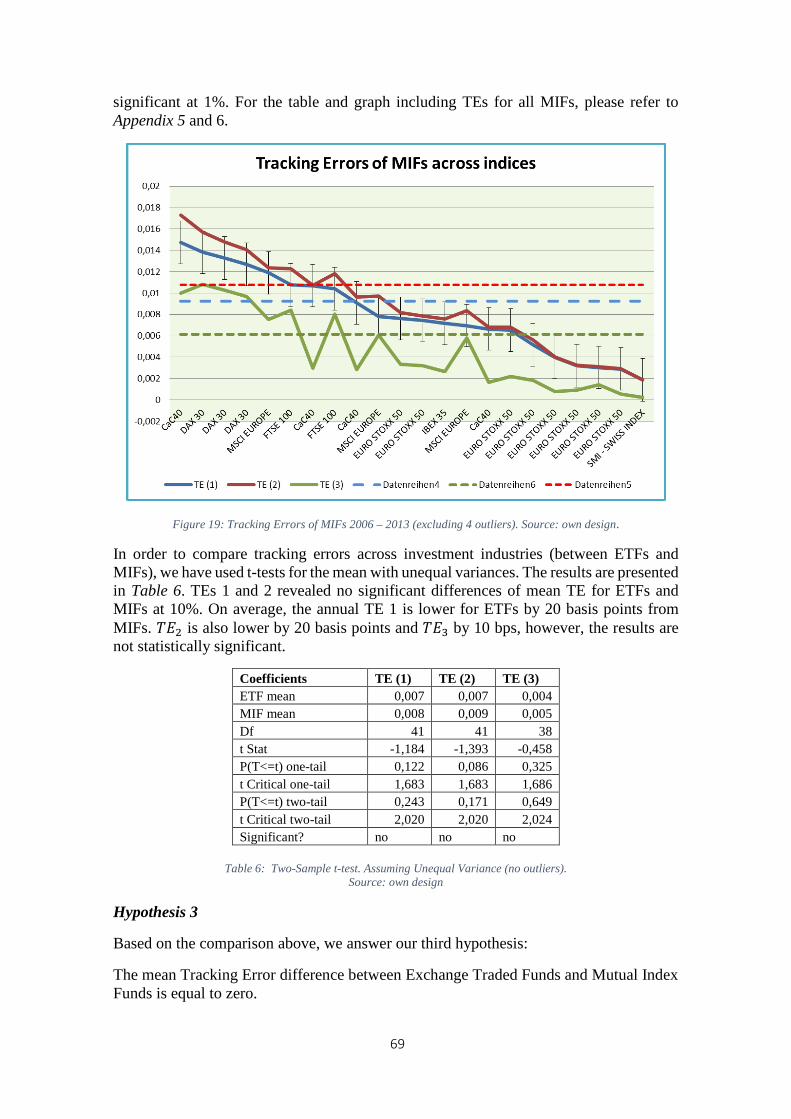
significant at 1%. For the table and graph including TEs for all MIFs, please refer to Appendix 5 and 6.

Figure 19: Tracking Errors of MIFs 2006 – 2013 (excluding 4 outliers). Source: own design.

In order to compare tracking errors across investment industries (between ETFs and MIFs), we have used t-tests for the mean with unequal variances. The results are presented in Table 6. TEs 1 and 2 revealed no significant differences of mean TE for ETFs and MIFs at 10%. On average, the annual TE 1 is lower for ETFs by 20 basis points from MIFs. 𝑇𝑇𝑇𝑇2 is also lower by 20 basis points and 𝑇𝑇𝑇𝑇3 by 10 bps, however, the results are not statistically significant.

Coefficients TE (1) TE (2) TE (3) ETF mean 0,007 0,007 0,004 MIF mean 0,008 0,009 0,005 Df 41 41 38 t Stat -1,184 -1,393 -0,458 P(T<=t) one-tail 0,122 0,086 0,325 t Critical one-tail 1,683 1,683 1,686 P(T<=t) two-tail 0,243 0,171 0,649 t Critical two-tail 2,020 2,020 2,024 Significant? no no no

Table 6: Two-Sample t-test. Assuming Unequal Variance (no outliers).

Source: own design

Hypothesis 3

Based on the comparison above, we answer our third hypothesis:

The mean Tracking Error difference between Exchange Traded Funds and Mutual Index Funds is equal to zero.

69

𝐻𝐻0: 𝑇𝑇𝑇𝑇𝑀𝑀𝑀𝑀 − 𝑇𝑇𝑇𝑇𝐸𝐸𝐸𝐸𝑀𝑀 = 0

𝐻𝐻𝑁𝑁: 𝑇𝑇𝑇𝑇𝑀𝑀𝑀𝑀 − 𝑇𝑇𝑇𝑇𝐸𝐸𝐸𝐸𝑀𝑀 ≠ 0

Given the results for Tracking Error 1-3, we accept H0. There was no statistical evidence that mean Tracking Errors of ETFs and MIFs differ from each other. This is in accordance with previous research by Rompotis (2005), Svetina and Wahal (2008) and Agapova (2011) performed on the U.S. and cross-national markets.

5.4.3. Annual Comparison of Tracking Errors

Hypothesis 3 told us that over a longer period of time, TE difference becomes insignificant. We now intend to find out if this result also holds for a shorter investment period. To develop further knowledge about this relationship, we compare Tracking Errors of MIF and ETF on a yearly basis to see whether the tracking performance is constant for both funds over time. At first, we would like to present an overview of daily TEs by years and then compare them. Figure 20 shows the average TE, calculated according to method 2, for ETFs and MIFs.

Figure 20: Tracking Error Comparison, ETFs (blue), MIFs (red), no outliers. Source: own design.

As visible on Figure 20, 𝑇𝑇𝑇𝑇2 increased during 2008 for both, ETFs and MIFs. The increase for ETFs was 44 and 13 bps from the average during 2008 and 2009 respectively, and 60 and 15 basis points for MIFs.5 Although weaker, another breaking point for both fund types can be observed during 2010. The bottoms and peaks in 2008 and 2010 are likely to be attributed to high turbulence caused by the U.S. mortgage crisis of 2008 and by the European debt crisis triggered in 2010. Displaying the annual Tracking Error as done in Figure 21 below depicts an even clearer picture of the events.

The annual Tracking Errors are in line with the daily ones, as can be seen by comparing Figure 20 above and Figure 21 below. Both graphs indicate that ETFs tend to have slightly smaller TEs than MIFs.

5 𝑇𝑇𝑇𝑇3 draws a similar picture and will therefore not be discussed in detail.

70

0,060,09

0,18

0,120,10 0,10

0,070,07

0,09

0,24

0,160,13

0,17

0,11

2006 2007 2008 2009 2010 2011 2012

Annual TE 2TE 2 ETF TE 2 MIF

Figure 21: Annual Tracking Errors 2006 – 2013. Source: Own design

In order to test the impressions from the graphs above, we applied t-tests for the mean tracking error on the annual basis. Table 7 shows the results based on TE method 2.

Table 7: Annual 𝑇𝑇𝑇𝑇2 t tests (no outliers). Source: own design

Against the impression from Figure 21, we found no significant differences between MIFs and ETFs from 2006 to 2010. The years of 2011 until the end of 2012 signal that there were differences and ETFs performed better than MIFs based on 𝑇𝑇𝑇𝑇2using both annual and daily rate. In 2011 the difference was 40 bps (5% significance level) in favor of ETFs and 20 bps (10%) in 2012. Significant results obtained only for the last two years of the studied period cannot signal that ETFs perform better than MIFs in terms of tracking; thus we conclude that both ETFs and MIFs have on average the same TEs on a yearly basis. Summary We compared TEs calculated by three different methods across ETFs and MIFs, including and excluding outliers as mentioned in the previous chapter. First TEs analysis with outliers resulted in significant difference among ETFs and MIFs in terms of TEs for the whole period and each year. Second, analysis excluding outliers revealed no significant difference. Table 8 presents the results of our comparison:

Year 2006 2007 2008 2009 2010 2011 2012Coefficients TE (2) TE (2) TE (2) TE (2) TE (2) TE (2) TE (2)ETF mean 0,055 0,092 0,177 0,124 0,097 0,102 0,074MIF mean 0,069 0,093 0,237 0,164 0,129 0,166 0,105t Stat -1,08 -0,04 -1,58 -1,37 -1,50 -2,57 -1,96P one-tail 0,14 0,49 0,06 0,09 0,07 0,01 0,03t Crit one-tail 1,69 1,68 1,69 1,68 1,68 1,69 1,69P two-tail 0,29 0,97 0,12 0,18 0,14 0,01 0,06t Crit two-tail 2,03 2,02 2,02 2,02 2,02 2,03 2,03Significant at No No No No No 5% 10%

71

Check Betas TE 1(SSE) TE 2(stdv) TE 3(MAD)

with outliers

Long-term difference?

yes yes yes yes

Different per year? n/a n/a yes

Evidence for 2008 and

2011(10%) excluding 4 outliers

Long-term difference? no no no no

Different per year? no no Evidence for 2011-2012 no

Table 8: Results of Tracking Error comparison. Source: own design.

We checked whether ETFs perform better tracking in comparison to MIFs using two sample t-tests for unequal variance. “Long-term difference” represents the comparison using comprising results for the whole span of 2006 – 2013, “different per year” indicates whether there were differences for the chosen variables among each year separately.

In a nutshell, we show that tracking errors in the long, as well as in the short run are moving around the same mean for both investment tools with a slight indicator for lower TEs of Exchange Traded Funds throughout the last two years. The yearly investigation of TE further suggests that they might be influenced by certain events that affected the economy in the past. This relationship will be analyzed in detail throughout chapter 5.3.4.

Excursus: Discussion of Outliers In the following, we discuss outliers which we dismissed from the main comparison and tests when comparing TEs.

*all intercepts t-ratios are statistically insignificant, thus intercepts are not different from zero

Table 9 above presents original results of regression and results after using a Moving Average model of a span of 100 on 1825 observations. We used the MA model in order to smooth high frequency data (daily returns for 7 years) and obtain a comprehensible picture of funds’ performance. In addition, MA models could deliver better results in the case of high autocorrelation of returns. All outcomes of the MA model are significant and prove that chosen indices track their benchmark; however, they perform their job poorly on a daily basis. These results are consistent with Frino and Gallagher (2001) and Chu

Table 9: Regression of outliers with their benchmarks. Source: Own design.

72

(2011), who reported that TEs calculated as using daily returns are usually high in comparison to those TEs which are calculated using monthly data. For example, Frino and Gallagher studied ETFs index tracking performance relative to S&P500 using monthly returns with obtained betas no lower than 0,99 and accordingly quite low TEs. In contrast, Chu (2011) used daily returns with obtained betas varying between 0,99 and -0,0009. His research was aimed on ETFs tracking main Chinese indices. Moreover, it is worth to note that Chu studied funds replication using a span of one year in most of the cases and Frino and Gallagher’s studied span was five years.

These are analyses of outliers and reasons behind bad performance of funds selected as outliers (in total 4 funds all are MIFs):

• ING Direct tracking CAC 40 has too low Betas and high TEs. First, its objective is to obtain an annual TE of less than 1% or to keep it below 5% of CAC 40’s volatility. We found that it is ranked with the lowest mark according to quantanalyst.com and boursorama.com (all are representative independent fund analysis providers). In addition, ING Direct had difficulties tracking CAC 40 after March of 2009 due to high turbulences on the market caused by the U.S. financial crisis and the beginning of debt crisis in EU. One can observe from the Figure 19 below that quality of tracking was appropriate before 2009 and decreased after 2009 during upward moves in CAC 40. This is consistent with the studies of Blitz et al. (2012) and Chiang (1998), stating that funds obtain a higher TE during upward trends of the index and track well during its decline.

Figure 22: ING Direct and CAC 40 2006-2013. Source: Own design

• AEX’s BNPParibas had low tracking performance, because its main objective was to track Euronext All Share (it is a more comprehensive index including Euronext AEX index). Although AEX and AEX all share are similar on average using monthly data, we exclude them from our analysis of TEs as we use daily data. For details, please see the Figure 23 below.

73

Figure 23: AAX (AEX all share) and AEX index, 2007 – 2013. Source: Own design

• Etoile Gestion Mutual Fund changed its objective to seek the maximum performance using stock picking, thus becoming actively managed. Euro Stoxx index was used for the Etoile Gestion Mutual Fund only as a benchmark to evaluate the performance of the mangers. We exclude this index from our study since it is actively managed (Etoile, 2013, p.1).

• Lux Euro Stock Mutual Fund tracking TecDax performed badly due to the same reason as ING Direct tracking CAC40; it had difficulties keeping up with the growing index after 2009. The difficulties set in after 2007 and increased significantly after 2009 due to the U.S. financial crisis, which increased volatility of markets. Please see the Figure 24 below.

Figure 24: Lux Euro (black) and TecDax index (blue), 2007 – 2013. Source: Own design

To sum up, based on our analysis of TE1 (using standard errors of residuals) and betas as an estimation of tracking performance of ETFs and MIFs, we can conclude that there was

74

no significant difference in TE1 between ETFs and MIFs during 2006 and 2013. Our findings for European index trackers are similar with Rompotis (2005) and Agapova (2011).

5.4.4. Market State and Tracking Error

We have divided the overall time frame of 7 years into four sub-periods (please see 4.1.1 Time Horizon) according to the different market states. The sub-periods capture several different moods of the European economy as measured by the MSCI Europe. Figures 25 and 26 below show the development of the MSCI Europe and tracking errors respectively over the whole time horizon between 2006 and 2013. We used yearly averages of 𝑇𝑇𝑇𝑇2 and 𝑇𝑇𝑇𝑇3 for ETFs and MIFs6.

A comparison of both graphs (Figures 25 and 26) generates the impression of opposing movement between the European market and fund tracking error in a way that if the market descends, the tracking error starts to increase in the same time. Together with the fact that tracking error decreases while the market seems to recover, we already assume that tracking error is negatively correlated with the index movement and thus tracking quality increases during booms, while it seems to decrease during recessions. To gain evidence about the relationship between market return and TE, we regressed 𝑇𝑇𝑇𝑇2 and 𝑇𝑇𝑇𝑇3 against MSCI Europe index returns. Doing so, the results for both methods

6 The reason why we exclude 𝑇𝑇𝑇𝑇1 from this test is that it is based on the standard error of regression. To obtain TE-values for the years 2006-2007 we would need to run regressions for 47 funds for 7 years, which means 47*7=329 additional regressions and therefore would exceed our schedule.

Figure 25: MSCI Europe yearly average (2006-2013). Figure 26: Average TEs (2006-2013).

75

turned out to be significant. The strongest relationship, however, evolved from the regression using 𝑇𝑇𝑇𝑇2.

Table 10 illustrates the outcome of this regression analysis for ETF and MIF respectively. In both cases the alpha coefficients are positive (around 5%) and significant within the 5% level. Beta-coefficients are -0,52 and -0,33 for ETFs and MIF respectively and also significant at the 5% level. R² are 60% and 63,4% respectively. Those values indicate a clear negative relationship between the tested variables, while it seems to be slightly stronger for MIFs.

Sub-Periods Figure 27 and 28 illustrate the respective Tracking Error in relation to the MSCI Europe return during the different periods between 2006 and 2013. The red line shows rolling annual average of 𝑇𝑇𝑇𝑇2 and the blue line illustrates the average returns of MSCI Europe. The lines clearly indicate a reverse movement between both variables. Using the evidence from the regression in combination with Figure 27 and 28 we can investigate the behavior of index tracking during the different sub-periods.

Figure 27: Regression TE and MSCI Europe for ETF. Source: Own design

Table 10: Regression of TE and MSCI. Source: Own calculation

Name ETF TE and MSCI MIF TE and MSCIMultiple R 0,78 0,80

R^2 0,60 0,63SE 0,02 0,02

Intercept 0,06 0,05t ratio 2,69(5%) 2,87(5%)

TE (2) Ann. -0,52 -0,37t ratio 2,74(5%) 2,94(5%)

76

Figure 28: Regression TE and MSCI Europe for MIF. Source: Own design

Period 1: Dec. 2006 to Dec. 2007, declining returns after the boom. Period 2: Jan. 2008 to Feb. 2009, strong recession (subprime mortgage crisis), marked green. Period 3: Mar. 2009 to 2010, ascending trend (recovering phase) Period 4: Jan. 2010 to Dec. 2012, stagnation (European sovereign debt crisis), marked green.

Period 1: The first sections in the graphs show the mean change of the yearly TE and index returns from the end of 2006 to the beginning of 2008. The blue line reflects the decrease in average returns during the year 2007 even though the overall upwards trend was not broken until 2008; there was already a decline in 2007. With the ups and downs during the year, Tracking Errors slightly increase for both instruments by the same value.

Period 2: The actual recession started in the beginning of 2008 as a result of the financial crisis and lasted until the beginning of 2009. For the index, this is shown by a strong decrease in returns during this time. Simultaneously, the slope of TEs strongly increases. We can observe that the Mutual Index Fund TE increases by 100% compared to 145% for Exchange Traded Fund TE.

Period 3: From March 2009 onwards, the market started to recover, and so did Tracking Errors for both investment instruments. Even though index returns reached pre-crisis levels again, TEs have not recovered to the base date level. While ETF Tracking Error evens out at 4% above base date level, MIF Tracking Error recovers to 6% above base date.

Period 4: Recovery in 2010 was slowed down and changed into stagnation due to the European sovereign debt crisis. For the following years, the European market showed several smaller ups and downs which might indicate the uncertainty of the future development. On average, the level remains fairly constant over time. At first the drop in Tracking Errors slows down. Next, between 2011 and 2013, they vary antithetic to market returns. While the Tracking Error for ETFs averages at 10%, MIFs once again react strongly to the market decline in mid-2011.

77

Hypothesis 4

For ETFs: There is no correlation between mean Tracking Error and the European economy.

𝐻𝐻0: 𝛽𝛽𝐸𝐸𝐸𝐸𝑅𝑅𝐸𝐸𝐸𝐸𝐸𝐸𝐸𝐸𝐸𝐸 = 0

𝐻𝐻𝑁𝑁: 𝛽𝛽𝐸𝐸𝐸𝐸𝑅𝑅𝐸𝐸𝐸𝐸𝐸𝐸𝐸𝐸 ≠ 0

Hypothesis 5

For MIFs: There is no correlation between mean Tracking Error and the European economy.

𝐻𝐻0: 𝛽𝛽𝐸𝐸𝐸𝐸𝑅𝑅𝐸𝐸𝐸𝐸𝐸𝐸𝐸𝐸𝐸𝐸 = 0 𝐻𝐻𝑁𝑁: 𝛽𝛽𝐸𝐸𝐸𝐸𝑅𝑅𝐸𝐸𝐸𝐸𝐸𝐸𝐸𝐸 ≠ 0 What is visualized by Figure 27 and 28 is verified by the regression results in Table 10; therefore we can state that changes in Tracking Errors of European Index Trackers are clearly correlated to the movement of European markets. We see that Index Funds in the form of ETFs and MIFs, which track European indices, do a better job during booming or recovering development and deliver a poorer tracking quality during recessions. We further demonstrate that Mutual Index Funds tend to be stronger affected by this relationship than corresponding ETFs. The results are in accordance with previous research on ETF Tracking Error, as conducted by Blitz and Huji (2012), Rompotis (2006, 2011), Aber et al. (2009) and others, who show that ETF Tracking Error is positively correlated with market volatility. We extended the previous results by showing a significant increase in Tracking Error during crises, not only for European ETFs but also for Mutual Index Funds on European indices.

5.5. Total Expense Ratio

5.5.1. ETF vs. MIF

As the descriptive statistics at the beginning of this chapter show, there are no significant differences in returns between index tracker and benchmark index. The two fund models therefore have a substitutive character (cf. Agapova, 2011) and thus, if replicating the same index, can be seen as direct competitors, who, amongst others, have to compete via their price, which is reflected by fund fees. Given similar return characteristics, we are now going to investigate whether either ETFs or MIFs are able to operate more cost efficiently than the respective counterpart. As previously discussed, we use Total Expense Ratio to represent fund fees as passed on to the investor.

78

Table 11: Average of TER by index. Source: Own calculation

Table 11 shows the average values for ETFs and MIFs expense ratios7. We can see that the average TER for Mutual Index Funds (1,11%) exceeds the average expenses of ETFs (0,3%) by a notable 0,8%. Respective t-tests (Appendix 7) show that the differences are significant within the 1% level. Figure 29 shows Expense Ratios of both fund types grouped up by indices.

Figure 29: TER for ETFs and MIF grouped for Index. Source: Own design

We can see that MIF expenses are frequently higher than those of ETFs with two exceptions; Credit Suisse produces lower fees when tracking the Swiss Market Index (SMI) than iShares and the FTSE 100 tracker of HBSC has lower costs than the respective ETF of UBS. In both cases we are talking about a difference of 10 bps.

7 Please note that for the calculation of average TER we removed two outlier Mutual Index Funds: ING Direct CAC 40 and Morgan Stanley Liberty Spanish. We excluded these two values as they break away by nearly 1% from the rest of the sample. Therefore, we find this funds rather distorting than representative for the whole sample. The exclusion reduces the average TER for MIFs by 7 bps.

Name ETF MIFAEX 0,003 0,006CaC40 0,003 0,015DAX 30 0,002 0,007EURO STOXX 50 0,002 0,012FTSE 100 0,004 0,006FTSE DEVELOPED EUROPE 0,001IBEX 35 0,003MSCI EUROPE 0,003 0,009S&P EURO 0,004SMI 0,004 0,004TECDAX (XETRA) 0,005 0,018Average of TER 0,003 0,011

79

Hypothesis 6:

The difference of mean TER for Exchange Traded Funds and Mutual Index Funds is equal to zero

𝐻𝐻0: 𝑇𝑇𝑇𝑇𝑅𝑅𝑀𝑀𝑀𝑀 − 𝑇𝑇𝑇𝑇𝑅𝑅𝐸𝐸𝐸𝐸𝑀𝑀 = 0

𝐻𝐻𝑁𝑁: 𝑇𝑇𝑇𝑇𝑅𝑅𝑀𝑀𝑀𝑀 − 𝑇𝑇𝑇𝑇𝑅𝑅𝐸𝐸𝐸𝐸𝑀𝑀 ≠ 0

Since the difference in Total Expense Ratio between ETF and MIF is significantly different from zero, we have to reject 𝐻𝐻0.

Our findings about TER generally confirm the results of most of the previously conducted research also for European index trackers, i.e. that ETFs have on average lower expense ratios than MIFs. Blitz et al. (2010, p. 655) state TERs for ETFs between 0,35% and 0,75% and for MIFs between 0,38% and 1,22% for different international benchmarks. Rompotis (2005, p. 13) calculated an average of 0,228% for ETFs and 0,423% for MIFs, and Agapova (2011, p. 328) states average expense ratios of 0,18 for ETFs and 0,75% for MIFs. We observe only two examples, where MIF beat ETF expense ratios. It appears that the company which operates in the country the benchmark is related to can operate more cost efficient than the respective ETF provided by a foreign investment company

5.5.2. Total Expense Ratio and Tracking Error

We observed that for the most funds, Mutual Index Funds charge higher fees to the investor than Exchange Traded Funds. Since our final quality criteria for index fund performance is Tracking Error, we are trying to work out if there is a relationship between fees and tracking quality. Hypothesis 7 and 8 give an idea about the impact magnitude of TER on TE that an investor should consider when making the choice for either one of the investment instruments. Table 12 contains the results of the regressions with Tracking Error as dependent and Total Expense Ratio as explanatory variable. The regression was run for 𝑇𝑇𝑇𝑇1 to 𝑇𝑇𝑇𝑇3 separately and for both fund types combined as well as individually. Section A shows the regression including the pool of all funds, section B only including ETFs and section C MIFs.

Table 12: Regression TE with TER. Source: Own design.

The constants for all regressions are slightly positive and significant between the 1% or 10% level. Coefficients for TER are positive for section B, negative for section C and varying for different Tacking Errors in section A. The t-values, however, show that only the coefficient for 𝑇𝑇𝑇𝑇3 in section C is significant at the 5% level. Yet, the graph in

Coefficient

Type TE (1) TE (2) TE (3) TE (1) TE (2) TE (3) TE (1) TE (2) TE (3)Alpha 0,007 0,007 0,005 0,006 0,006 0,003 0,010 0,010 0,008t stat 7,76* 7,71* 6,41* 2,84** 2,74** 2,04*** 4,87* 4,88* 4,7*TER 0,038 0,042 -0,087 0,344 0,410 0,415 -0,119 -0,173 -0,283t stat 0,39 0,39 1,09 0,55 0,62 0,94 0,79 1 2,19**R^2 0,004 0,004 0,028 0,016 0,020 0,045 0,030 0,050 0,190SSE 0,004 0,004 0,003 0,004 0,004 0,003 0,004 0,004 0,003

B. Regression of ETFs C. Regression of MIFsA: Regression of all investment vehicles

80

Appendix 8 shows that the results are not normally distributed and therefore cannot be taken as valid.

Based on the data from Table 12 we answer hypothesis 7-8:

Hypothesis 7

There is no correlation between Total Expense Ratio and Mutual Index Fund Tracking Error.

𝐻𝐻0: 𝛽𝛽𝐸𝐸𝐸𝐸𝐸𝐸𝐸𝐸𝑅𝑅 = 0

𝐻𝐻𝑁𝑁: 𝛽𝛽𝐸𝐸𝐸𝐸𝐸𝐸𝐸𝐸𝑅𝑅 ≠ 0

Hypothesis 8

There is no correlation between Total Expense Ratio and Exchange Traded Fund Tracking Error.

𝐻𝐻0: 𝛽𝛽𝐸𝐸𝐸𝐸𝐸𝐸𝐸𝐸𝑅𝑅 = 0

𝐻𝐻𝑁𝑁: 𝛽𝛽𝐸𝐸𝐸𝐸𝐸𝐸𝐸𝐸𝑅𝑅 ≠ 0

In contrast to Meinhardt et al. (2012), we cannot use expense ratios to explain ETFs Tracking Error. The same applies for the regression result using MIFs. Due to the lack of significance, we accept 𝐻𝐻0 for both hypothesis 7 and hypothesis 8 and state that we cannot observe an effect of TERs on neither ETFs nor MIFs Tracking Error and therefore TER has no influence on tracking quality of neither of them. This might be due to the small amount of observations we make when splitting up the fund categories, which also enjoins us with the task of generalizing the findings about the relationship between TE and TER. It is therefore recommended to repeat the regression with a more comprehensive sample for both fund categories.

81

5.6. Executive Summary

Hypothesis # Formulation Accept Null Hypothesis?

Hypothesis 1 𝐻𝐻0: µ𝑀𝑀𝑀𝑀 − µ𝐼𝐼𝑛𝑛𝑑𝑑𝐼𝐼𝐼𝐼 = 0

𝐻𝐻𝑁𝑁: µ𝑀𝑀𝑀𝑀 − µ𝐼𝐼𝑛𝑛𝑑𝑑𝐼𝐼𝐼𝐼 ≠ 0

Hypothesis 2 𝐻𝐻0: µ𝐸𝐸𝐸𝐸𝑀𝑀 − µ𝐼𝐼𝑛𝑛𝑑𝑑𝐼𝐼𝐼𝐼 = 0

𝐻𝐻𝑁𝑁: µ𝐸𝐸𝐸𝐸𝑀𝑀 − µ𝐼𝐼𝑛𝑛𝑑𝑑𝐼𝐼𝐼𝐼 ≠ 0 Hypothesis 3

𝐻𝐻0: 𝑇𝑇𝑇𝑇𝑀𝑀𝑀𝑀 − 𝑇𝑇𝑇𝑇𝐸𝐸𝐸𝐸𝑀𝑀 = 0

𝐻𝐻𝑁𝑁: 𝑇𝑇𝑇𝑇𝑀𝑀𝑀𝑀 − 𝑇𝑇𝑇𝑇𝐸𝐸𝐸𝐸𝑀𝑀 ≠ 0 Hypothesis 4 For ETFs: �

𝐻𝐻0:𝛽𝛽𝐸𝐸𝐸𝐸𝑅𝑅𝐸𝐸𝐸𝐸𝐸𝐸𝐸𝐸𝐸𝐸 = 0HA: 𝛽𝛽𝐸𝐸𝐸𝐸𝑅𝑅𝐸𝐸𝐸𝐸𝐸𝐸𝐸𝐸 ≠ 0

Hypothesis 5 For MIFs: �

𝐻𝐻0:𝛽𝛽𝐸𝐸𝐸𝐸𝑅𝑅𝐸𝐸𝐸𝐸𝐸𝐸𝐸𝐸𝐸𝐸 = 0HA: 𝛽𝛽𝐸𝐸𝐸𝐸𝑅𝑅𝐸𝐸𝐸𝐸𝐸𝐸𝐸𝐸 ≠ 0

Hypothesis 6

𝐻𝐻0: 𝑇𝑇𝑇𝑇𝑅𝑅𝑀𝑀𝑀𝑀 − 𝑇𝑇𝑇𝑇𝑅𝑅𝐸𝐸𝐸𝐸𝑀𝑀 = 0

𝐻𝐻𝑁𝑁: 𝑇𝑇𝑇𝑇𝑅𝑅𝑀𝑀𝑀𝑀 − 𝑇𝑇𝑇𝑇𝑅𝑅𝐸𝐸𝐸𝐸𝑀𝑀 ≠ 0 Hypothesis 7 For MIFs: �𝐻𝐻0:𝛽𝛽𝐸𝐸𝐸𝐸𝐸𝐸𝐸𝐸𝑅𝑅 = 0

HA: 𝛽𝛽𝐸𝐸𝐸𝐸𝐸𝐸𝐸𝐸𝑅𝑅 ≠ 0

Hypothesis 8 For ETFs: �𝐻𝐻0:𝛽𝛽𝐸𝐸𝐸𝐸𝐸𝐸𝐸𝐸𝑅𝑅 = 0HA: 𝛽𝛽𝐸𝐸𝐸𝐸𝐸𝐸𝐸𝐸𝑅𝑅 ≠ 0

Table 13: Overview of Hypothesis outcomes. Source: Own design.

6. Conclusion In this chapter we restate and answer our research question from chapter 1. We base the answer on the findings discussed throughout chapter 5 and draw a conclusion about how the research purpose was fulfilled and what the main practical and theoretical contributions of this paper are. We end with a number of interesting recommendations for further studies that connect to our research and would pick up on our delimitations.

The purpose of this paper was to identify and estimate measures for tracking quality within the passive fund industry and compare them within the two investment instruments Mutual Index Funds and Exchange Traded Funds. We extended existing knowledge on the matter by exclusively appreciating index funds with European benchmarks and provide a basis for more extensive research within the field. As a basis for the study, we formulated our research question as follows.

82

RQ: Do Exchange Traded Funds replicate the Performance of European Indices better than Mutual Index Funds?

To gain sufficient knowledge that allows us to answer this questions and the related hypotheses, we accomplished a number of test procedures that led us to inferring that

- neither Exchange Traded Funds nor Mutual Index Funds show tracking quality advantage when compared to each other.

We therefore answer the main research question with “no”.

Over the period of 2006 to the end of 2012, both instruments on average achieved their objective, i.e. to deliver the same return as the benchmark index. This was shown by the insignificance of return differences between the fund types, as well as between funds and indices. The main evidence for tracking quality, however, was found by comparing the tracking errors of both instruments. Yet again, for the timeframe in question we found no significant difference testifying that the overall tracking quality is the same for both instruments. This fact does also not change when we switch from the long term to a yearly perspective. 𝑇𝑇𝑇𝑇2 was the only estimate that slightly indicated an advantage of ETFs for the last two years of our test period. Even though, we are not inferring any conclusive statement from this, it might be interesting to continue following the trend over the next years.

We further took the recent turmoils on global and European markets as an opportunity to see how tracking error behaves during different market states. Therefore the first sub question of our research problem was the following:

SQ 1: Is tracking quality correlated with the states in European financial markets?

Our answer to this question is “yes”. We were able to show a clear negative relationship between market movement and tracking error which means that index tracking risk increases during recession and vice versa. We found this to be true for both instruments with slightly stronger evidence for Mutual Index Funds.

Investigating similar products with substitutional features, we tried to work out if there is a price difference in the form of unequal expense ratios with the following sub-question:

SQ 2: Is there a difference in fund costs?

We show in our study that MIFs have frequently higher expense ratios than ETFs (on average 80 bps), which is in accordance with most research on other markets. However, in our case, the investigation of impacts of fees on Tracking Error does not allow for any statistical inference.

Overall, our results lead us to the conclusion, that index investment instruments, namely Exchange Traded Funds and Mutual Index Funds on European indices, on average provide a satisfying tracking quality without showing significant quality differences in achieving their goal in the long term. Their yearly comparison with the European market further indicates that both instruments show deficits in tracking accuracy during down markets, while this phenomenon is stronger for Mutual Index Funds. Furthermore, even though we found that on average, MIFs show higher fees, we cannot prove any related impact on tracking performance.

83

Based on our results, we agree that Mutual Index Funds and Exchange Traded Funds with the objective of tracking European indices are good, however not perfect, substitutes when tracking the same benchmark (cf. Agapova, 2011; Svetina & Wahal, 2008). While both deliver approximately the same tracking performance, it mainly depends on the investor and his objectives to decide whether to invest in ETF or MIF.

6.1. Theoretical and Practical Contribution

The number of studies directly comparing Mutual Index Funds and Exchange traded funds is still limited, mainly due to the emerging state of Exchange Traded Funds, which made it difficult in the past to obtain a sufficient amount of observations. Our study ties in on previous research and contributes to the subject by allowing for the generalization of knowledge to European index trackers. We not only provide new evidence about the development on the so far neglected European market, but also give an update on the field by using the most recent available data. By analyzing tracking performance, fee distribution and market correlation, we give a new and comprehensive insight into Index Funds in the form of Exchange Traded Funds and Mutual Index Funds. We provide feasible results for each investment instrument separately, as well as in a comparative manner which can be taken as a basis for further theoretical and practical purposes.

From a practical perspective, our results can be considered not only by current and future investors who have or consider making investments in the European market, but also by both sides of investment companies.

First, investors who struggle with the understanding of the difference between these two very similar investment instruments can complement their knowledge, and based on their preferences consider our findings for decision making. While a long-term investor, for instance, might be rather indifferent between ETFs and MIFs, apart from tradability, our findings suggest a preference for ETFs for short-term investors due to lower fees and a lower sensitivity towards short term changes in the European market.

Secondly, our results indicate a highly substitutional relationship between ETFs and MIFs. Investment companies therefore might consider our outcomes for strength and weaknesses investigation in order to pursue their competitiveness. We show that both, ETFs and MIFs, show inferior tracking during down markets which should give incentive for improvement. Further, ETFs tend to beat passive mutual funds in cost efficiency, which has important implications for fund managers as fees are a frequent decision criteria for passive investors.

6.2. Further Research Suggestion

We see reason to continually update the knowledge of our research subject. This is mainly due to the ongoing growth of the ETF market and the implied increasing amount of data availability, which will promote higher research flexibility in the future. It will remain interesting to monitor the coexistence of MIFs and ETFs and to follow current trends. Future questions for research projects might be whether ETFs keep gaining market shares and whether there will be further improvements (e.g. we found weak evidence for short term tracking improvement of ETFs when compared to MIFs). We would like to motivate researchers to not only renew previous findings and to explore further markets, but also to take our results as a basis for a cross-sectional investigation, e.g. to expose possible differences between the well investigated U.S. fund market and Europe trackers.

84

We further recommend an in-depth analysis of more factors that affect tracking quality of index funds on European markets. This might be done by using logistic regression, as introduced throughout this work. Including more factors such as expense ratios, fund volume, fund age and others that have a potential impact on tracking in combination with a higher amount of observations would further contribute to the understanding of differences between ETFs and MIFs on the European Market.

Such a casual study could also have an exclusive focus on Exchange Traded Funds. As we have seen throughout chapter 3, ETFs make use of different methods to replicate indices (namely physical and synthetical replication). Since the replication method is at the heart of index tracking, there is a substantial ongoing debate on which of the methods is superior. It would therefore be valuable to continue this discussion within our population of European index trackers.

Another direction for further research might be to focus on the more specialized sector funds, which are also available to investors in the form of MIFs as well as ETFs. These more “exotic” tracker funds provide a variety of additional investment possibilities and became of increasing importance in the recent past. Due to the extensive diversification of the instruments across market sectors, they provide a lot of food for thought

85

Reference List

ABDC. (2013). ABDC Journal Ratings List. Australian Business Deans Council web site. <http://www.abdc.edu.au/3.43.0.0.1.0.htm> [Retrieved March 7, 2013]

Aber, J. W., Li, D., Can, L. (2009). Price volatility and tracking ability of ETFs. Journal of Asset Management (2009) 10, 210-221.

Abner, D. J. (2010). The ETF handbook how to value and trade exchange-traded funds. Hoboken, N.J.: Wiley.

ABDC. (2013). Australian Business Deans Council | ABDC Journal Ratings List. ABDC web site. <http://www.abdc.edu.au/3.43.0.0.1.0.htm> [Retrieved 2013-03-08]

Abner, D. J. (2010). The ETF Handbook: How to Value and Trade Exchange Traded Funds (1st Ed.). Wiley.

Adams, J., Khan, H. T. A., Raeside, R., & White, D. I. (2007). Research Methods for

Graduate Business and Social Science Students. SAGE Publications Pvt. Ltd.

Adelmeyer, M., & Warmuth, E. (2005). Finanzmathematik für Einsteiger: Von Anleihen über Aktien zu Optionen. Springer DE.

AEX. (2013). AEX Famiy Rules. NYSE Euronext. <https://indices.nyx.com/en/products/indices/NL0000000107-XAMS> [Retrieved 2013-04-07]

Agapova, A. (2011). Conventional mutual index funds versus exchange-traded funds. Journal of Financial Markets, 14(2), 323–343. doi:10.1016/j.finmar.2010.10.005

Amenc, N., Goltz, F., Martellini, L., & Ye, S. (2011). Improved Beta? A Comparison of Index-Weighting Schemes. EDHEC-Risk Institute, 1(1), 5-49.

Ammann M. & Zimmermann H. (2001) Tracking Error and Tactical Asset Allocation, Financial Analysts Journal, 57(2), March/April, 32-43.

Anderson, S. C., Born, J. A., & Schnusenberg, O. (2010). Closed-end funds, exchange-traded funds, and hedge funds: origins, functions, and literature. New York: Springer.

Armstrong, D. B. (2011). 3 Problems with the S&P 500 Index. Money web site. <http://money.usnews.com/money/blogs/the-smarter-mutual-fund-investor/2011/03/04/3-problems-with-the-sp-500-index> [Retrieved 2013-04-26]

Arnott, R. D., Hsu, J., & Moore, P. (2005). Fundamental Indexation. Financial Analysts Journal, 61(2), 83-99.

x

Bamberg, G., & Wagner, N. (2000). Equity index replication with standard and robust regression estimators. OR Spectrum, 22(4), 525–543.

BlackRock. (2010). ETF Industry Highlights 2010. Blackrock web site. <http://www.blackrockinternational.com/content/groups/internationalsite/documents/literature/etfl_industryhilight_ye10.pdf> [Retrieved 2013-03-15]

BlackRock. (2012). ETP Landscape Dec. Blackrock web page. <http://www2.blackrock.com/ca/en/InstitutionalInvestors/MarketInsight/etflandscape/index.htm > [Retrieved 2013-04-07]

BlackRock. (2013). ETP Landscape Jan. Blackrock web page. <http://www2.blackrock.com/ca/en/InstitutionalInvestors/MarketInsight/etflandscape/index.htm [Retrieved 2013-04-07]

Blitz, D., Huij, J. (2012). Evaluating the Performance of Global Emerging Markets Equity Exchange-Traded Funds. Available at <http://ssrn.com/abstract=1757740>

Blitz, D., Huij, J., & Swinkels, L. (2010). The Performance of European Index Funds and Exchange-Traded Funds. European Financial Management, 18(4), 649-662.

Bloomberg (2013). List of Index Fund Funds Worldwide. Bloomberg - Business, Financial & Economic News, Stock Quotes. Bloomber web site. <http://www.bloomberg.com/markets/funds/index-fund/> [Retrieved 2013-05-01].

Blume, M. E., & Edelen, R. M. (2002). On replicating the S&P 500 index. Rodney L. white center for financial research-working papers.

Bollen, N. B., & Pool, V. K. (2012). Suspicious Patterns in Hedge Fund Returns and the Risk of Fraud. Review Of Financial Studies, 25(9), 2673-2702.

Bryman, A., & Bell, E. (2007). Business research methods (2nd ed.). Oxford: Oxford Univ. Press.

Bryman, A., & Bell, E. (2011). Business research methods (3rd ed.). Oxford: Oxford Univ. Press.

Burrell, G., & Morgan, G. (1992).Sociological paradigms and organisational analysis: elements of the sociology of corporate life. Aldershot: Ashgate.

BVI. (2010). BVI - Wohlverhaltensregeln. BVI web site. <http://www.bvi.de/fileadmin/user_upload/Statistik/TER_auszug.pdf> [Retrieved 2013-04-07]

Cambro (2013). Cambro Portal. Web site. < www.cambro.umu.se/portal> [Retrieved 2013-02-10]

CFA (2012). Program Curriculum. Charlottesville, Va.: CFA Institute

xi

Chu Patrick Kuok-Kun (2011). Study on the tracking errors and their determinants: evidence from Hong Kong exchange traded funds. Applied Financial Economics,21(5).

Cottrell, A. (2003). Regression analysis: basic concepts. Regression. From <http://www.ecn.wfu.edu/~cottrell/ecn215/regress_jw.pdf> [Retrieved 2013-04-07]

Cowton, Christopher J. (1998). The use of secondary data in business ethics research. Journal of Business Ethics 17 (4), 423-434.

Cooper, D. R., & Schindler, P. S. (2008). Business research methods (10th ed.). Boston: McGraw-Hill Irwin.

Dale, A., & Arber, S. (1988). Doing secondary analysis. London: Unwin Hyman.

Datastream. (2008). Datastream quality of Time Series. Datastream Time Series. UWE web site. <www2.uwe.ac.uk/services/library/your_subject/Business%20and%20management/datastreamdataquality.pdf> [Retrieved 2013-03-04]

Db X-trackers. (2013). Deutsche Asset & Wealth Management - Exchange Traded Funds - db X-trackers. db X-trackers web site. <http://www.etf.db.com/DE/DEU/Pages/Disclaimer/132.html?pketf=70&pageid=143&forwardurl=/DE/DEU/ETF/LU0322250985/DBX1AR/CAC_40%C2%AE_UCITS_ETF.html> [Retrieved 2013-03-26]

Denscombe, M. (1998). The good research guide for small-scale social research projects (2nd ed.). Maidenhead: Open University Press.

Deutsche Bank Research. (2008). Exchange Traded Funds - Hohes Wachtumspotential dank innovativer ETF-Strukturen. Deutsche Bank Research web site. <http://www.dbresearch.de/PROD/DBR_INTERNET_DE-PROD/PROD0000000000224386.pdf> [Retrieved 2013-04-07]

Deville, L. (2008). Exchange Traded Funds: History, Trading, and Research. Handbook of Financial Engineering, 67-98. Springer.

Di Tollo, G., & Maringer, D. (2009). Metaheuristics for the index tracking problem. Metaheuristics in the Services Industry, 624, 127-154.

EBSCO. (2013). Business Source Premier | Business magazines and journals | EBSCO. EBSCO web site <http://www.ebscohost.com/academic/business-source-premier> [Retrieved 2013-03-07]

Easterby-Smith, M., Thorpe, R., & Jackson, P. (2012). Management research (4th ed.). Los Angeles: Sage.

Ehmann, A. (2008). Ein DAX-ETF aus japanischen Aktien? Morningstar UK website. <http://www.morningstar.de/de/news/41346/ein-dax-etf-aus-japanischen-aktien.aspx> [Retrieved 2013-03-26]

xii

Elton, E. J., Gruber, M. J., Brown, S. J., & Goetzmann, W. N. (2010). Modern Portfolio Theory and Investment Analysis: International Student Version (8. Auflage.). John Wiley & Sons.

Elton, E. J., Gruber, M. J., Comer, G., & Li, K. (2002). Spiders: Where Are the Bugs? Journal of Business, 75(3), 453-472.

Eriksson, P., & Kovalainen, A. (2008).Qualitative methods in business research. Los Angeles: SAGE.

Etoile (2013). Etoile Factsheet. Kiidline web site. <http://www.kiidline.com/documents/2013/02/18/KID_ETOILE_EURO_OPPORTUNITES_CL11206_FRA_FR.pdf> [Retrieved 2013-04-29]

Ferri, R. A. (2009). The ETF Book: All You Need to Know About Exchange-Traded Funds (Updated Edition.). John Wiley & Sons.

Frino, A., & Gallagher, D. R. (2001). Tracking S&P 500 Index Funds. The Journal of

Portfolio Management, 28(1), 44–55. doi:10.3905/jpm.2001.319822.

Fry, D. H. (2008). Create your own ETF hedge fund: a do-it-yourself ETF strategy for private wealth management. Hoboken, N.J.: John Wiley & Sons.

Fuller, R. J., Bing Han, & Yining Tung. (2010). Thinking about Indices and “Passive” versus Active Management. Journal of Portfolio Management, 36(4), pp. 35–47.

Gabelli, M.J. (2002). The History of Hedge Funds. The Millionaire's Club.

Gastineau, G. L. (2004). The benchmark index ETF performance problem. The Journal of Portfolio Management, 30(2), 96-103.

Ghauri, P. N., & Grønhaug, K. (2005). Research methods in business studies: a practical guide (3rd ed.). Harlow, England: Financial Times Prentice Hall.

Ghorawat, N. (2013). A Critique on Equating Growth in Market Indices to Returns on Equity Investments. CA. Nirmal Ghorawat web site. From <http://canirmalg.wordpress.com/2013/03/0> [Retrieved: 2013-05-22].

Gill, J., & Johnson, P. (2010). Research methods for managers (4th ed.). Los Angeles: SAGE.

Grix, J. (2002). Introducing Students to the Generic Terminology of Social Research. Political Studies Association, 22(3), 175-186.

Guedj, I., & Huang, J. (2008). Are ETFs replacing index mutual funds? Working paper. University of Texas at Austin.

Hehn, E. (2005). Exchange Traded Funds: Structure, Regulation and Application of a New Fund Class (1th ed.). Springer.

xiii

Heidorn, T., Löw, C., & Winker, M. (2010). Funktionsweise und Replikationstil europäischer Exchange Traded Funds auf Aktienindices. Working Paper series. No. 139. Frankfurt School of Finance & Management.

Henry, G. T. (1990). Practical Sampling. SAGE.

Herring, F., & Hunke, T. (2001). Investmentfonds und Kostentransparenz. Zeitschrift für das gesamte Kreditwesen, (16/17), 906-909.

Howell, D. (2009). Statistical Methods for Psychology, International Edition (International edition.). Wadsworth.

Huff, A. S. (2009). Designing Research for Publication. Thousand Oaks: Sage Publications.

Hübscher, M. (2005). The Role of Exchange Traded Funds in the Active vs. Passive Debate. In: E. Hehn, Exchange Traded Funds (pp. 71–83). Springer web site. <http://link.springer.com/content/pdf/10.1007/3-540-27637-8_6> [Retrieved 2013-04-13]

Hwang & Satchell (2001) Tracking Error: Ex-Ante versus Ex-Post Measures. Journal of Asset Management, 2, (3), 1 December 2001, pp. 241-246(6).

iShares. (2012). Growth of ETF. iShares web site. <http://au.ishares.com/about_ishares/growth_ishares.do> [Retrieved 2013-02-14]

Ivanov, S. I. (2012). REIT ETFs performance during the financial crisis. Journal Of Finance & Accountancy, pp. 101-9.

John E. Cresson, R. Mike Cudd, Tom J. Lipscomb, (2002). The early attraction of S&P index funds: is perfect tracking performance an illusion? Managerial Finance, 28 (7), 1 - 8

Jordan, B. D., & Miller, T. W. (2009). Fundamentals of investments: valuation and management. Boston: McGraw-Hill/Irwin.

Khang, H., Ki, E., & Ye, L. (2012). Social Media Research in Advertising, Communication, Marketing, and Public Relations, 1997–2010. Journalism & Mass Communication Quarterly, 89(2), 279-298.

Khorana, A., Servaes, H., & Tufano, P. (2009). Mutual Fund Fees around the World. The Review of Financial Studies, 22(3), 1279-1310. doi:10.2307/30225692.

Klapper, L., Sulla, V., & Vittas, D. (2004). The development of mutual funds around the world. Emerging Markets Review, 5(1), 1-38.

Koop, G. (2006). Analysis of Financial Data. John Wiley & Sons.

Kostovetsky, L. (2003). Index Mutual Funds and Exchange-Traded Funds. The Journal of Portfolio Management, 29(4), 80-92. doi:10.3905/jpm.2003.319897.

xiv

Larsen, G.A. Jr and Resnick, B.G. (1998), “Empirical insights on indexing”,Journal of Portfolio Management, 25 (1), 51-60.

Lawton-Browne, C. (2001). An alternative calculation of tracking error. Journal ofAsset Management, 2(3), 223–234.

Leveraged ETFs. (2009). SEC web site. <http://www.sec.gov/investor/pubs/leveragedetfs-alert.htm> [Retrieved 2013-02-21]

Larsen, G.A. Jr and Resnick, B.G. (1998), “Empirical insights on indexing”,Journal of Portfolio Management, Vol. 25 No. 1, 51-60.

Lawton-Browne, C. (2001). An alternative calculation of tracking error. Journal ofAsset Management, 2(3), 223–234.

Leveraged ETFs. (2009). SEC web site. <http://www.sec.gov/investor/pubs/leveragedetfs-alert.htm> [Retrieved 2013-02-21]

LIBRIS. (2013). About Libris. LIBRIS web site. <http://librishelp.libris.kb.se/help/about_libris_eng.jsp?open=about> [Retrieved 2013-03-07]

Louargant, C., Neuberg, L., & Terraza, V. (2006). Time lags in fund of funds. Derivatives Use, Trading & Regulation, 12(3), 190-199.

McGlone, M. (2011). Understanding commodities and the s&p gsci®. Technical report, Standard and Poors. S&P Dow Jones Indices web site. <http://findout.spindices.com/documents/education/practice-essentials-understanding-commodities-gsci.pdf> [Retrieved 2013-04-13]

Meinhardt, C., Müller, S., & Schöne, S. (2012). Synthetic ETFs: Will Full Replication Survive? (SSRN Scholarly Paper No. ID 2026409). Rochester, NY: Social Science Research Network.

Meziani, A. S. (2006). Exchange-traded Funds as an Investment Option. Palgrave Macmillan.

Moore, D., McCabe G., Duckworth W. M. and Alwen L. (2011). The Practice of Statistics for Business and Economics. (3rd ed.). New York: W.H. Freeman.

Moore, L. M. (1996). The basic practice of statistics. Technometrics, 38(4), 404–405.

Morningstar. (2013a). Expense Ratio. Morningstar web site. <https://admainnew.morningstar.com/webhelp/glossary_definitions/mutual_fund/glossary_all_Expense_Ratio.html> [Retrieved 2013-04-13]

Morningstar (2013b). On the right track. Morningstar web site. <http://media.morningstar.com/uk/MEDIA/Research_Paper/Morningstar_Report_Measuring_Tracking_Efficiency_in_ETFs_February_2013.pdf> [Retrieved 2013-04-13]

xv

MSCI (2013). MSCI Europe Index factsheet. MSCI web site. <http://www.msci.com/resources/factsheets/index_fact_sheet/msci-europe-index.pdf > [Retrieved 2013-05-17].

Mutual Fund Ratings. (2013) Mutual Fund, ETF Investment Research. Morningstart web site. <http://www.morningstar.com/Cover/Funds> [Retrieved 2013-04-13].

Pope, F. Peter and Pradeep K. Yadav (1994). Discovering Errors in Tracking Error, Journal of Portfolio Management, 20(2), 27-32.

Remenyi, D., Williams, B., Money, A., & Schwartz, E. (1998). Doing research in business and management: an introduction to process and method. London: Sage.

Robson, C. (2002). Real world research: a resource for social scientists and practitioner-researchers (2nd ed.). Oxford, UK: Blackwell Publishers.

Roll R. (1992) ‘A Mean/Variance Analysis of Tracking Error’, The Journal of Portfolio Management, 18 (4), Summer, 13–22.

Rompotis, G. (2005). An Empirical Comparing Investigation on Exchange Traded Funds and Index Funds Performance. Available at SSRN 903110. <http://papers.ssrn.com/sol3/papers.cfm?abstract_id=903110> [Retrieved 2013-04-13]

Rompotis, G. (2006). Evaluating the Performance and the Trading Characteristics of iShares. University of Athens. Available at SSRN: http://ssrn.com/abstract=946732 or http://dx.doi.org/10.2139/ssrn.946732 [Retrieved 2013-04-13]

Rompotis G. (2008). Performance and Trading Characteristics of German Passively Managed ETFs. International Research Journal of Finance and Economics, 15.

Rompotis G. (2011). Predictable patterns in ETFs' return and tracking error. Studies in Economics and Finance, 28(1), 14-35.

Rudolf M., Hans-Jürgen Wolter, Heinz Zimmermann,(1999). A linear model for tracking error minimization, Journal of Banking & Finance, Volume 23, Issue 1, J, Pages 85-103, ISSN 0378-4266, 10.1016/S0378-4266(98)00076-4.

Ruppert, D. (2011). Statistics and data analysis for financial engineering. New York: Springer.

Saunders, M., Lewis, P., Thornhill, A. (2007). Research methods for business students (4th ed.). Harlow, England: Financial Times/Prentice Hall.

Saunders, M., Lewis, P., Thornhill, A. (2009). Research methods for business students (5. ed.). Harlow, England: Financial Times/Prentice Hall.

SEC. (2007). Index Funds. SEC web site. <http://www.sec.gov/answers/indexf.htm> [Retrieved 2013-02-18]

xvi

SEC. (2010a). Exchnage Traded Funds. SEC web site. <http://www.sec.gov/answers/etf.htm> [Retrieved 2013-02-18]

SEC. (2010b). Mutual Funds. SEC web site. <http://www.sec.gov/answers/mutfund.htm> [Retrieved 2013-02-20]

Sharifzadeh, M., & Hojat, S. (2012). An analytical performance comparison of exchange-traded funds with index funds: 2002–2010. Journal of Asset Management, 13(3), 196-209.

Shaw, R. (2008). Three Approaches to Index Weighting. Seeking Alpha - Stock Market News & Financial Analysis . Seeking Aplpha web site. From <http://seekingalpha.com/article/95466-three-approaches-to-index-weighting>. [Retrieved: 2013-05-22].

Spindices. (2013). S&P 500 Index - S&P Dow Jones Indices. S&P Dow Jones Indices web site. <http://eu.spindices.com/indices/equity/sp-500> [Retrieved 2013-03-26]

S&P 500. (2012). S&P Dow Jones Indices: Index Mathematics Methodology. S&P Dow Jones Indices: Index Methodology, 1-59. S&P Dow Jones Indices web site. <https://www.sp-indexdata.com/idp/LoginAction.do> [Retrieved 2013-03-20]

Standard and Poor’s. (2012). S&P Dow Jones Indices. The McGraw-Hill Companies. S&P web site. <http://www.standardandpoors.com/servlet/BlobServer?blobheadername3=MDT-Type&blobcol=urldata&blobtable=MungoBlobs&blobheadervalue2=inline%3B+filename%3Dfs-sp-500-ltr.pdf&blobheadername2=Content-Disposition&blobheadervalue1=application%2Fpdf&blobkey=id&blobheadername1=content-type&blobwhere=1244142397091&blobheadervalue3=UTF-8> [Retrieved 2013-04-13]

STOXX (2013). Euro STOXX 50®. STOXX web site. < http://www.stoxx.com/indices/index_information.html?symbol=sx5E> [Retrieved 2013-05-21]

Svetina, M., & Wahal, S. (2008). Exchange traded funds: Performance and competition. Working Paper. Available at SSRN 1303643. <http://papers.ssrn.com/sol3/Delivery.cfm?abstractid=1303643> [Retrieved 2013-04-13]

Tashakkori, A., & Teddlie, C. (1998). Mixed Methodology: combining qualitative and quantitative approaches. Thousand Oaks, Calif. etc.: Sage Publications, Inc.

Tashakkori, A., & Teddlie, C. (Eds.). (2002). Handbook of Mixed Methods in Social &

Behavioral Research. Sage Publications, Inc.

Tobe C. (1999) ‘Tracking Error: An Essential Tool in Evaluating Index Funds’, The Journal of Investment Consulting, 2 (November), 8–11.

xvii

Umeå School of Business and Economics, Department of Business Administration (2012). Thesis writing in Business Administration, Umeå School of Business, Umeå University, Umeå, Sweden

Umeå Universitetsbibliotek (2013). Datastream | Umeå universitetsbibliotek. Umeå University Library web site. <http://proxy.ub.umu.se:2058/en/search/journals/datastream> [Retrieved 2013-03-07]

Upton, G. J., & Cook, I. (2008). A dictionary of statistics (2nd ed.). Oxford: Oxford University Press.

Wagner, N. (2002). Passives Management: Methoden zum Tracking von Marktindizes. 2002, 813–839.

xviii

Appendix 1: List of Fund pairs with matching Indices

Index Pair(ETF 1st)DAX Lyxor and PioneerSTOXX Lyxor and GesbankiMSCI EU Lyxor and VangdSTOXX SPDR and DBVSTOXX SPDR and SwisscantoSMI UBS and CSFTSE UBS and HSBCSTOXX UBS and Vital GestionCAC40 Amundi and StrategieIBEX BBVA and MSSTOXX DBX and UnionFTSE Ishares and HalifaxDAX Ishares and OppenheimSTOXX Ishares and InversafCAC 40 Lyxor and MAM

xix

Appendix 2: T-tests for mean return difference T-tests for the mean return difference, daily based on 2006 - 2013 Source: Own calculation

Index Name of a Fund Type Mean of Mean of index t stat Significant? Obs.AEX BNP MIF -0,0001 -0,0001 0,009 no 1825AEX SPDR ETF -0,0001 -0,0001 0,000 no 1825AEX IHARES ETF -0,0001 -0,0001 0,002 no 1825CAC40 Lyxor ETF -0,0001 0,0000 -0,273 no 1825CAC40 Amundi ETF -0,0001 0,0000 -0,095 no 1825CAC40 ING.DRCT. MIF -0,0001 0,0000 -0,234 no 1825CAC40 NATIXIS MIF -0,0001 0,0000 -0,268 no 1825CAC40 MAM FRANCE MIF -0,0001 0,0000 -0,136 no 1825CAC40 STRATEGIE MIF -0,0001 0,0000 -0,264 no 1825CAC40 GESTION VALOR MIF -0,0001 0,0000 -0,124 no 1825DAX30 ISHARES ETF 0,0002 0,0002 -0,245 no 1680DAX30 LYXOR ETF 0,0002 0,0002 -0,089 no 1680DAX30 OPPENHEIM MIF 0,0001 0,0002 -0,117 no 1680DAX30 DT.POSTBANK MIF 0,0001 0,0002 -0,098 no 1680DAX30 PIONEER MIF 0,0002 0,0002 -0,062 no 1680EURO STOXX 50 INVERSAFEI BOLSA MIF -0,0001 -0,0002 0,576 no 1825EURO STOXX 50 VITALGESTION MIF -0,0001 -0,0002 0,583 no 1825EURO STOXX 50 GESBANKINTER MIF -0,0001 -0,0002 0,790 no 1825EURO STOXX 50 DBV WINTERTH.FD.MAN.CO. MIF -0,0001 -0,0002 0,387 no 1825EURO STOXX 50 MS ING DIRECT NARANJA MIF -0,0001 -0,0002 0,180 no 1825EURO STOXX 50 MORGAN STANLEY LBRTY. MIF -0,0001 -0,0002 0,059 no 1825EURO STOXX 50 UNION INVESTMENT LX. MIF -0,0001 -0,0002 0,332 no 1825EURO STOXX 50 ETOILE EURO MIF -0,0001 -0,0002 0,657 no 1825EURO STOXX 50 KBC INDEX MIF -0,0001 -0,0002 0,648 no 1825EURO STOXX 50 ISHARES ETF -0,0002 -0,0002 0,992 no 1825EURO STOXX 50 UBS ETF -0,0002 -0,0002 0,576 no 1825EURO STOXX 50 Lyxor ETF -0,0002 -0,0002 0,974 no 1825EURO STOXX 50 SPDR ETF -0,0001 -0,0002 0,712 no 1825EURO STOXX 50 DBX UCITS ETF ETF -0,0003 -0,0002 0,001 no 1825FTSE 100 HALIFAX MIF 0,0001 0,0000 0,485 no 1762FTSE 100 HSBC MIF 0,0000 0,0000 0,531 no 1762FTSE 100 ISHARES ETF -0,0001 0,0000 0,997 no 1762FTSE 100 ISHARES ETF 0,0000 0,0000 0,333 no 1762FTSE 100 UBS ETF -0,0003 0,0000 0,483 no 1762IBEX 35 BBVA ACCION ETF -0,0003 -0,0003 0,192 no 1597IBEX 35 MORGAN STANLEY LIBERTY MIF -0,0002 -0,0003 0,309 no 1597MSCI EUROPE VANGD MIF -0,0001 -0,0001 0,715 no 1689MSCI EUROPE AMUNDI MIF 0,0000 -0,0001 0,837 no 1689MSCI EUROPE SWISSCANTO CH MIF -0,0001 -0,0001 0,928 no 1689MSCI EUROPE LYXOR ETF -0,0001 -0,0001 0,130 no 1689MSCI EUROPE SPDR ETF 0,0000 -0,0001 0,624 no 1689SMI CREDIT SUISSE CSA MIF 0,0000 -0,0001 0,337 no 1689SMI ISHARES ETF 0,0001 -0,0001 0,001 no 1689SMI UBS ETF -0,0001 -0,0001 0,431 no 1689SMI Credit Suisse ETF 0,0000 -0,0001 0,371 no 1689TECDAX LUX EURO MIF 0,0001 0,0002 0,440 no 1825TECDAX ISHARES ETF 0,0002 0,0002 0,827 no 1825

xx

Appendix 3: Two-sample t-test for ETF and MIF t-Test: Two-Sample Assuming Unequal Variances for ETF and MIF over or underperformance between each other

Appendix 4: Results of logistic regression (15 pairs) 1) Significant at 10% values are in bold.

Index IBEX CAC 40 STOXX FTSE

Test BBVA and MS

Lyxor and MAM

Lyxor and Gesbanki

UBS and HSBC

Hos. and Lem. Test 0,39 0,60 0,08 0,48

Correct prediction,% 70,83 61,11 54,17 62,50

Coefficient for single const -0,88 -0,45 -0,16 0,51

Sig. 0,00 0,06 0,48 0,04

Unconditional OR for ETFs 0,41 0,64 0,84 1,67

Nagelkerke R Square 0,27 0,14 0,07 0,06

Coefficient (Return) -20,27 13,04 -7 -10,96

Sig. 0,00 0,01 0,15 0,08

OR 0,00 5,20 0,93 0,00

95% CI lower 0,00 20,33 0,74 0,00

95% CI upper 0,00 57,00 1,02 4,50

Coefficient (Stdev) -84,50 -52 -69,41 -44

Index CAC 40 CAC 40 Dax Dax Stoxx Stoxx Stoxx Stoxx FTSE 100 FTSE 100 IBEX MSCI EU MSCI EU SMI

Name

Lyxor and Mam France

Amundi and Strategie

Ishares and Oppenheim

Lyxor and Pioneer

Ishares and Iversafei

Lyxor and Vital Gestion

SPDR and Gesbanki

Dbx and DBV

Ishares DE and Halifax

Ishares and HSBC

BBVA and MS

Lyxor and Vanguard

SPDR and Amundi

Ishares and CS

Mean ETF( -0,038 -0,014 0,043 0,049 -0,044 -0,044 -0,023 -0,071 -0,030 -0,006 -0,087 -0,029 0,006 0,021Mean MIF -0,019 -0,037 0,041 0,047 -0,017 -0,020 -0,015 -0,049 0,022 -0,004 -0,060 -0,033 0,005 0,008Observatio 1825 1825 1680 1680 1825 1825 1825 1562 1762 1762 1597 1689 1689 1825df 3557 3648 3356 3355 3637 3624 3587 3122 3433 3517 3184 3211 3376 3614t Stat -0,13 0,17 0,02 0,01 0,21 0,19 -0,05 -0,15 -0,37 -0,01 -0,18 0,03 0,00 0,13P one-tail 0,45 0,43 0,49 0,50 0,42 0,42 0,48 0,44 0,36 0,49 0,43 0,49 0,50 0,45t Crit. one 1,65 1,65 1,65 1,65 1,65 1,65 1,65 1,65 1,65 1,65 1,65 1,65 1,65 1,65P two-tail 0,90 0,86 0,99 0,99 0,84 0,85 0,96 0,88 0,71 0,99 0,86 0,98 1,00 0,90t Crit. two 1,96 1,96 1,96 1,96 1,96 1,96 1,96 1,96 1,96 1,96 1,96 1,96 1,96 1,96Significantno no no no no no no no no no no no no no

xxi

Sig. 0,06 0,43 0,08 0,26

OR 0,00 0,00 0,00 0

95% CI lower 0,00 0,00 0,00 0

95% CI upper 8,31 7,23 14,00 0

Coefficient (Constant) 0,064 -0,44 0,41 1,09

Sig. 0,92 0,08 0,68 0,06

OR 1,06 0,64 1,51 2,97

2) All results from logistic regression

Index CAC40 IBEX STOXX FTSE DAX STOXX CAC 40

Name

Amundi and Strategie

BBVA and MS

DBX and Union

Ishares and Halifax

Ishares and Oppenheim

Ishares and Inversaf

Lyxor and MAM

Constant Single B -0,38 -0,88 -0,36 1,42 1,34 -0,22 -0,45

Sig. 0,10 0,00 0,10 0,00 0,00 0,35 0,06

Exp(B) 0,67 0,41 0,67 4,14 3,80 0,80 0,64

Goodness of Fit

Percentage Correct 59,72 70,83 59,72 80,56 79,17 55,56 61,11

-2 Log likelihood 93,89 71,98 96,08 70,48 72,81 98,53 88,52

Cox & Snell R Square 0,04 0,19 0,01 0,01 0,01 0,01 0,10

Nagelkerke R Square 0,06 0,27 0,02 0,01 0,02 0,01 0,14

higher better

Hosmer and Lemeshow Test 0,79 0,39 0,95 0,07 0,64 0,50 0,60

Return B 7,54 -

20,27 1,42 -2,73 -0,35 1,19 13,04

S.E. 5,18 6,26 4,62 7,28 5,51 4,52 5,11

Wald 2,12 10,49 0,09 0,14 0,00 0,07 6,50

xxii

df 1,00 1,00 1,00 1,00 1,00 1,00 1,00

Sig. 0,15 0,00 0,76 0,71 0,95 0,79 0,01

Exp(B) 1,80 0,00 4,15 0,07 0,70 3,29 5,20

95% C.I.for EXP(B) 0,07 0,00 0,00 0,00 0,00 0,00 20,33

Upper 47,96 0,00 3,58 10,14 3,44 2,32 103,34

Stdev B -4,97 -

84,50 -26,02 -30,55 39,59 -13,50

S.E. 39,13 44,19 37,37 44,49 51,21 35,40

Wald 0,02 3,66 0,48 0,47 0,60 0,15

df 1,00 1,00 1,00 1,00 1,00 1,00

Sig. 0,90 0,06 0,49 0,49 0,44 0,70 0,44

Exp(B) 0,01 0,00 0,00 0,00 15,60 0,00

95% C.I.for EXP(B) 0,00 0,00 0,00 0,00 0,00 0,00

Upper 139,20 7,23 32,20 39,50 25,00 0,00

Constant B -0,30 0,06 0,00 1,82 0,80 -0,01 -0,44

S.E. 0,62 0,68 0,59 0,67 0,74 0,57 0,26

Wald 0,23 0,01 0,00 7,48 1,15 0,00 2,99

df 1,00 1,00 1,00 1,00 1,00 1,00 1,00

Sig. 0,63 0,92 1,00 0,01 0,28 0,98 0,08

Exp(B) 0,74 1,07 1,00 6,17 2,22 0,99 0,64

Index DAX STOXX MSCI EU STOXX STOXX

Name

Lyxor and Pioneer

Lyxor and Gesbanki

Lyxor and Vangd

SPDR and DBV

SPDR and Swisscanto

Constant Single B 0,63 -0,17 1,95 -2,08 0,63

Sig. 0,01 0,48 0,00 0,00 0,01

Exp(B) 1,88 0,85 7,00 0,13 1,88

xxiii

Goodness of Fit

Percentage Correct 65,28 54,17 87,50 88,89 65,28

-2 Log likelihood 92,42 95,38 50,52 48,66 90,68

Cox & Snell R Square 0,01 0,05 0,05 0,02 0,03

Nagelkerke R Square 0,01 0,07 0,10 0,04 0,04

Hosmer and Lemeshow Test 0,66 0,08 0,01 0,83 0,51

Return B -2,52 -6,98 11,41 -3,66 5,36

S.E. 4,49 4,90 7,46 7,93 3,59

Wald 0,31 2,03 2,34 0,21 2,23

df 1,00 1,00 1,00 1,00 1,00

Sig. 0,58 0,15 0,13 0,64 0,14

Exp(B) 0,08 0,00 90,24 0,03 212,72

95% C.I.for EXP(B) 0,00 0,00 0,04 0,00 0,19

Upper -4,37 -4,02 18,15 -3,85 47,17

Stdev B 7,35 -69,41 113,24 -86,77 n/a

S.E. 37,79 39,64 74,60 78,76 n/a

Wald 0,04 3,07 2,30 1,21 n/a

df 1,00 1,00 1,00 1,00 n/a

Sig. 0,85 0,08 0,13 0,27 0,87

Exp(B) 15,48 0,00 15,10 0,00 n/a

95% C.I.for EXP(B) 0,00 0,00 0,00 0,00 n/a

Upper 22,70 14,00 21,30 0,00 n/a

Constant B 0,54 0,82 0,41 -0,90 0,67

S.E. 0,59 0,61 1,03 1,06 0,25

Wald 0,82 1,80 0,16 0,73 6,96

xxiv

df 1,00 1,00 1,00 1,00 1,00

Sig. 0,36 0,18 0,69 0,39 0,01

Exp(B) 1,71 2,28 1,51 0,41 1,96

Index SMI FTSE STOXX

Name UBS and CS UBS and HSBC

UBS and Vital Gestion

Constant Single B -0,51 0,51 -0,82

Sig. 0,04 0,04 0,00

Exp(B) 0,60 1,67 0,44

Goodness of Fit

Percentage Correct 62,50 62,50 69,44

-2 Log likelihood n/a 92,05 87,78

Cox & Snell R Square n/a 0,04 0,01

Nagelkerke R Square n/a 0,06 0,02

Hosmer and Lemeshow Test n/a 0,48 0,75

Return B n/a -10,96 -1,26

S.E. n/a 6,36 4,81

Wald n/a 2,97 0,07

df n/a 1,00 1,00

Sig. 0,76 0,08 0,79

Exp(B) n/a 0,00 0,28

95% C.I.for EXP(B) n/a 0,00 0,00

Upper 63,06 -4,50 -3,95

Stdev B n/a -44,36 23,94

xxv

S.E. n/a 39,90 36,36

Wald n/a 1,24 0,43

df n/a 1,00 1,00

Sig. 0,98 0,27 0,51

Exp(B) n/a 0,00 24,00

95% C.I.for EXP(B) n/a 0,00 0,00

Upper n/a 0,00 0,00

Constant B -0,51 1,09 -1,20

S.E. 0,24 0,57 0,61

Wald 4,40 3,61 3,90

df 1,00 1,00 1,00

Sig. 0,04 0,06 0,05

Exp(B) 0,60 2,97 0,30

Appendix 5: Tracking Errors of MIF

-0,005

0

0,005

0,01

0,015

0,02

0,025

Tracking Errors of MIFs across indices (all MIFs)

TE (1) TE (2) TE (3) Datenreihen4 Datenreihen6 Datenreihen5

xxvi

Appendix 6: Tracing Error (1), (2) and (3) for all Funds

Name Index Type TE (1) daily

TE (2) daily

TE (3) daily

TE (1) annual

TE (2) annual

Observations

SPDR AEX ETF 0,004 0,004 0,002 0,0691 0,069 1825ISHARES AEX ETF 0,003 0,003 0,002 0,0538 0,054 1825BNP PARIBAS AEX MIF 0,015 0,021 0,014 0,2663 0,371 1825LYXOR CaC40 ETF 0,003 0,003 0,001 0,0495 0,050 1825AMUNDI CaC40 ETF 0,004 0,004 0,002 0,0615 0,062 1825ING.DRCT. LYXOR INTERNATIONAL CaC40 MIF 0,016 0,023 0,016 0,2743 0,398 1825NATIXIS ASSET MANAGEMENT CaC40 MIF 0,015 0,017 0,010 0,2574 0,302 1825MAM MEESCHAERT FCP CaC40 MIF 0,011 0,011 0,003 0,1866 0,187 1825STRATEGIE CaC40 MIF 0,007 0,007 0,002 0,1158 0,119 1825GESTION VALOR CaC40 MIF 0,009 0,010 0,003 0,1584 0,168 1825ISHARES DAX 30 ETF 0,006 0,006 0,004 0,0927 0,094 1680LYXOR DAX 30 ETF 0,007 0,007 0,004 0,1103 0,114 1680OPPENHEIM KPL.DAX WERTE DAX 30 MIF 0,013 0,015 0,010 0,2220 0,258 1680DT.POSTBANK ASTMGMT.DYM. DAX 30 MIF 0,014 0,016 0,011 0,2310 0,274 1680PIONEER INVESTMENTS AKTIEN DAX 30 MIF 0,013 0,014 0,010 0,2125 0,245 1680ISHARES EURO STOXX 50 ETF 0,006 0,006 0,004 0,1002 0,101 1825UBS EURO STOXX 50 ETF 0,015 0,016 0,009 0,2558 0,278 1825LYXOR EURO STOXX 50 ETF 0,008 0,009 0,005 0,1459 0,152 1825SPDR EURO STOXX 50 ETF 0,012 0,012 0,009 0,2105 0,216 1825DB X-tracker EURO STOXX 50 ETF 0,004 0,004 0,001 0,0582 0,058 1562INVERSAFEI BOLSA EURO EURO STOXX 50 MIF 0,007 0,008 0,003 0,1296 0,137 1825VITALGESTION EURO STOXX 50 MIF 0,005 0,006 0,002 0,0902 0,098 1825GESBANKINTER EURO STOXX 50 MIF 0,003 0,003 0,001 0,0530 0,054 1825DBV WINTERTH.FD.MAN.CO. EURO STOXX 50 MIF 0,003 0,003 0,001 0,0505 0,051 1825ING DIRECT EURO STOXX 50 MIF 0,008 0,008 0,003 0,1329 0,142 1825MORGAN STANLEY LBRTY. EURO STOXX 50 MIF 0,007 0,007 0,002 0,1138 0,119 1825UNION INVESTMENT LX. EURO STOXX 50 MIF 0,003 0,003 0,001 0,0560 0,057 1825ETOILE GESTION OPPORTUNITES EURO STOXX 50 MIF 0,016 0,019 0,013 0,2856 0,332 1825KBC INDEX EURO STOXX 50 MIF 0,004 0,004 0,001 0,0696 0,070 1825UBS FTSE 100 ETF 0,013 0,014 0,010 0,2291 0,234 1762ISHARES DE FTSE 100 ETF 0,011 0,012 0,007 0,1968 0,205 1762ISHARES FTSE 100 ETF 0,003 0,003 0,001 0,0461 0,046 1762HSBC FTSE 100 MIF 0,011 0,012 0,008 0,1845 0,214 1762HALIFAX UK FTSE 100 MIF 0,010 0,012 0,008 0,1782 0,207 1762BBVA IBEX 35 ETF 0,008 0,008 0,003 0,1280 0,131 1597MORGAN STANLEY LIBERTY IBEX 35 MIF 0,007 0,008 0,003 0,1171 0,132 1597LYXOR MSCI EUROPE ETF 0,006 0,008 0,005 0,1048 0,127 1689SPDR MSCI EUROPE ETF 0,006 0,008 0,006 0,1008 0,129 1689VANGD. ADMIRAL SHS. MSCI EUROPE MIF 0,012 0,012 0,008 0,1995 0,216 1689AMUNDI MSCI EUROPE MIF 0,008 0,010 0,006 0,1312 0,169 1689SWISSCANTO CH MSCI EUROPE MIF 0,007 0,008 0,006 0,1168 0,146 1689ISHARES SMI - SWISS INDEX ETF 0,007 0,008 0,005 0,1294 0,147 1825UBS SMI - SWISS INDEX ETF 0,005 0,005 0,003 0,0935 0,095 1825Credit Suisse SMI - SWISS INDEX ETF 0,003 0,003 0,002 0,0567 0,057 1825CREDIT SUISSE CSA SMI - SWISS INDEX MIF 0,002 0,002 0,000 0,0325 0,033 1825ISHARES TECDAX (XETRA) ETF 0,008 0,008 0,005 0,1386 0,139 1825LUX EURO STOCK TECDAX (XETRA) MIF 0,016 0,022 0,016 0,2733 0,390 1825Average ETF 0,007 0,007 0,004 0,116 0,122Average MIF 0,009 0,011 0,006 0,159 0,188

xxvii

Appendix 7: Total Expense Ratio t-test Total Expense Ratio t-Test: Two-Sample Assuming Unequal Variances MIF ETF Mean 0,01058 0,0029 Variance 1,9E-05 2E-06 Observations 22 23 Hypothesized Mean Difference 0 df 25 t Stat 7,86414 P(T<=t) one-tail 0,0000 t Critical one-tail 1,70814 P(T<=t) two-tail 0,0000 t Critical two-tail 2,05954

Appendix 8: Correlation Tracking Error and Total Expense Ratio

xxviii

Umeå School of Business and Economics

Umeå University

SE-901 87 Umeå, Sweden

www.usbe.umu.se